Astronomy & Astrophysics manuscript no. ms_2c c©ESO 2017February 28, 2017

The VLA-COSMOS 3 GHz Large Project:Cosmic evolution of radio AGN and implications for radio-mode

feedback since z ∼ 5

V. Smolcic1, M. Novak1, I. Delvecchio1, L. Ceraj1, M. Bondi2, J. Delhaize1, S. Marchesi3, E. Murphy4, E. Schinnerer5,E. Vardoulaki6, G. Zamorani7

1 Department of Physics, Faculty of Science, University of Zagreb, Bijenicka cesta 32, 10002 Zagreb, Croatia2 Istituto di Radioastronomia di Bologna - INAF, via P. Gobetti, 101, 40129, Bologna, Italy3 Department of Physics & Astronomy, Clemson University, Clemson, SC 29634, USA4 National Radio Astronomy Observatory, 520 Edgemont Road, Charlottesville, VA 22903, USA5 Max-Planck-Institut fur Astronomie, Konigstuhl 17, D-69117 Heidelberg, Germany6 Argelander Institut for Astronomy, Auf dem Hügel 71, Bonn, 53121, Germany7 INAF-Osservatorio Astronomico di Bologna, Via Ranzani 1, I - 40127 Bologna, Italy

Received ; accepted

ABSTRACT

Based on a sample of over 1, 800 radio AGN at redshifts out to z ∼ 5, with typical stellar masses within ∼ 3 × (1010− 1011) M⊙, and

3 GHz radio data in the COSMOS field we derive the 1.4 GHz radio luminosity functions for radio AGN (L1.4GHz ∼ 1022−1027 W Hz−1)

out to z ∼ 5. We constrain the evolution of this population using continuous models of pure density, and pure luminosity evolutionsfinding best-fit parametrizations of Φ∗ ∝ (1 + z)(2.00±0.18)−(0.60±0.14)z, and L∗ ∝ (1 + z)(2.88±0.82)−(−0.82±0.34)z, respectively, with a turn-overin number and luminosity densities of the population at z ≈ 1.5. Converting 1.4 GHz luminosity to kinetic luminosity, taking intoaccount uncertainties of the scaling relation used, we derive the cosmic evolution of the kinetic luminosity density provided by theAGN, and compare it to the radio-mode AGN feedback assumed in the "Semi-Analytic Galaxy Evolution" (SAGE) model, i.e. to theredshift evolution of the central supermassive black hole accretion luminosity taken in the model as the source of heating that offsetsthe energy losses of the cooling, hot halo gas, and thereby limits further stellar mass growth of massive galaxies. We find that thekinetic luminosity exerted by our radio AGN may be high enough to balance the radiative cooling of the hot gas at each cosmic epochsince z ∼ 5. However, although our findings support the idea of radio-mode AGN feedback as a cosmologically relevant process inmassive galaxy formation, many simplifications in both the observational and semi-analytic approaches still remain and need to beresolved before robust conclusions can be reached.

Key words. galaxies: fundamental parameters – galaxies: active, evolution – cosmology: observations – radio continuum: galaxies

1. Introduction

Understanding massive galaxy formation is one of the majorquests of modern astrophysics, and optimally studied via syn-ergy between theory (magnetohydrodynamic and semi-analyticsimulations) and (panchromatic) observations. Our current un-derstanding of massive galaxy formation requires energetic out-flows from radio-luminous active galactic nuclei (AGN) tosuppress stellar growth in the most massive galaxies (e.g.,Benson et al. 2003; Bower et al. 2006; Croton et al. 2006, 2016).This is mostly based on the advance of semi-analytic models inthe last decades.

Semi-analytic models are used to study the properties ofgalaxies formed in cosmological models within dark matter ha-los by describing ongoing physical processes, such as, e.g., gascooling, star formation, merger rates and various types of feed-back. One of their major past challenges was related to substan-tial overprediction of the quantity of the most massive galaxiesin the universe (see e.g. Steinmetz 1997). This was solved by in-troducing a process, dubbed ’radio-mode AGN feedback’ (e.g.,Croton et al. 2006).

By now radio-mode AGN feedback has become a standard,and key ingredient in semi-analytic models that allows repro-

ducing the observed galaxy properties well (Croton et al. 2006,2016; Bower et al. 2006; Sijacki et al. 2007). The feedback is as-sumed to be related to radio AGN outflows as the main sourcethat heats the halo gas surrounding a massive galaxy, and therebyquenching its star formation and limiting growth, thus avoidingcreating overly massive galaxies. Introducing such a feedbackprocess was motivated by radio AGN being observed to i) havemassive galaxy hosts (e.g. Best et al. 2005; Kauffmann et al.2008; Smolcic et al. 2009), and ii) interact with, i.e. heat theintra-cluster medium on large (group/cluster) scales potentiallysolving the so-called “cooling flow” problem in galaxy clusters(see Fabian 2012 for a review).

Initial implementations of radio-mode feedback were aimedat solving the cooling-flow problem, and generalized basedon simple phenomenological descriptions (Croton et al. 2006)or a sharp cutoff in cooling (Bower et al. 2006), both appliedbeyond a critical halo mass threshold. For example, in theCroton et al. (2006) model the source of heating was related tolow-luminosity radio activity caused by hot gas accretion ontothe central supermassive black hole (SMBH), once a static hothalo has formed around the host galaxy. The halo virial mass

Article number, page 1 of 13

A&A proofs: manuscript no. ms_2c

threshold beyond which a static hot halo forms was taken to be& 2.5 · 1011 M⊙ (see their Fig. 2).

A more complex cycle between gas cooling and the radio-mode AGN heating was recently implemented within theupdated Croton et al. (2006) model, i.e., the "Semi-AnalyticGalaxy Evolution" (SAGE) model (Croton et al. 2016). In thismodel cooling and heating of the halo gas has been more di-rectly coupled, and the phenomenological treatment of radio-mode feedback has been put on more physical grounds by as-suming accretion onto central SMBHs hosted by massive haloesof spherical, Bondi-Hoyle type (Bondi 1952), and scaled by aradio-mode efficiency parameter that modulates the strength ofthe accretion, and subsequently the radio-mode feedback.

From an observational point of view, radio-mode AGNfeedback, and particularly its cosmological relevance for mas-sive galaxy formation, as suggested by the semi-analytic mod-els, is difficult and challenging to test. While observationsof large, spatially resolved radio galaxies inducing cavities(i.e. buoyantly rising bubbles) in the hot X-ray emitting intra-cluster medium (ICM) are possible for a small number of wellstudied, nearby systems (e.g. Bîrzan et al. 2004; Bîrzan et al.2008; O’Sullivan et al. 2011), at higher redshifts the obser-vational data is limited as most of the systems are unre-solved in both, the radio and X-ray bands. This necessitatesthe use of scaling relations to convert the monochromatic ra-dio luminosity to kinetic luminosity, inferred either on the ba-sis of well studied nearby systems (Merloni & Heinz 2007;Bîrzan et al. 2008; Cavagnolo et al. 2010; O’Sullivan et al.2011; Godfrey & Shabala 2016), and assumed to hold at highredshifts (Smolcic et al. 2009; La Franca et al. 2010; Pracy et al.2016), or on theoretical grounds including various assump-tions drawn from well studied and resolved radio galaxies(Willott et al. 2001; Daly et al. 2012; Godfrey & Shabala 2016),and again assumed to hold for populations of radio AGN,observed in deep radio surveys over a large redshift range(Best et al. 2006, 2014).

A commonly used approach to estimate the cosmic evolu-tion of radio-mode feedback, i.e. that of the volume averaged ki-netic luminosity density of radio AGN, is based on constrainingthe cosmic evolution of radio AGN luminosity functions, con-volved with a scaling relation between the monochromatic andkinetic luminosities (Merloni & Heinz 2008; Cattaneo & Best2009; Smolcic et al. 2009; Smolcic et al. 2015; Best et al. 2014;Pracy et al. 2016). Hence, the cosmic evolution of radio AGNhas direct implications onto constraining the redshift evolutionof radio-mode AGN feedback.

Past studies have shown that radio AGN evolve differen-tially, consistent with cosmic downsizing: low radio-luminositysources evolve less strongly than high radio-luminosity sources,and the number density peak occurs at higher redshift for higher-luminosity radio AGN (Dunlop & Peacock 1990; Willott et al.2001; Waddington et al. 2001; Rigby et al. 2011). Consistentwith the evolution of optically and X-ray selected quasars (e.g.Schmidt et al. 1995; Silverman et al. 2008; Brusa et al. 2009),high luminosity radio AGN (L1.4GHz > 2 × 1026 W Hz−1) showa strong positive density evolution with redshift out to z ∼ 2,beyond which their comoving volume density starts decreas-ing (Dunlop & Peacock 1990; Willott et al. 2001). Intermediate,and low radio-luminosity AGN (L1.4GHz ∼ 1.6 × 1024

− 3 ×1026 W Hz−1) have been shown to evolve slower, with a co-moving volume density turnover occurring at a lower redshift(z ∼ 1 − 1.5; Waddington et al. 2001; Clewley & Jarvis 2004;Sadler et al. 2007; Donoso et al. 2009; Smolcic et al. 2009).

The goal of current studies is to constrain the cosmicevolution of the low-luminosity radio AGN reaching towardsthe epoch of reionization (z . 6; e.g. McAlpine et al. 2013;Smolcic et al. 2015; Padovani et al. 2015). This is becomingpossible only now via deep panchromatic surveys, including ra-dio data obtained with the recently upgraded radio facilities,such as the Karl. G. Jansky Very Large Array (VLA). In thiscontext, the VLA-COSMOS 3 GHz Large Project (Smolcic et al.2017b) is to-date the deepest radio continuum survey over arelatively large, 2 square degree field. Combined with the richCOSMOS multi-wavelength data (Scoville et al. 2007) it, thus,provides a unique data-set to study the evolution of the to-datefaintest observable radio AGN since z ∼ 5, and put the results incontext of radio-mode AGN feedback as an assumed cosmolog-ically relevant process for massive galaxy formation. This is theaim of the work presented here.

In Sect. 2 we describe the VLA-COSMOS 1.4 and 3 GHzprojects and the 3 GHz selected radio AGN sample used here.In Sect. 3 we derive the 1.4 GHz rest-frame radio luminos-ity functions for our AGN and model their evolution out toz ∼ 5. In Sect. 4 we consider the obtained results in the con-text of radio-mode AGN feedback, comparing them with theSAGE semi-analytic model, and in Sect. 5 we discuss variousunknowns remaining in both, the observational and analytic ap-proaches. We summarize in Sect. 6. Throughout the paper weadopt H0 = 70, ΩM = 0.3,ΩΛ = 0.7. We define the radio spec-tral index, α, via S ν ∝ ν

α, where S ν is the flux density at fre-quency ν. We use a Chabrier (2003) initial mass function.

2. Data and radio AGN sample

For our analysis we employ the VLA-COSMOS 3 GHz LargeProject (Smolcic et al. 2017b), as well as the VLA-COSMOS1.4 GHz Large and Deep Projects (Schinnerer et al. 2004, 2007,2010). The VLA-COSMOS 3 GHz Large Project provides ra-dio data at 10 cm wavelength within the COSMOS 2 square de-gree field down to an average (1σ) sensitivity of 2.3 µJy/beamover a 0.75′′ resolution element. The source catalog lists 10,830sources with signal-to-noise ratios (S/N) ≥ 5 (see Smolcic et al.2017b for details). Within the VLA-COSMOS 1.4 GHz LargeProject the 2 square degree COSMOS field has been observedwith the VLA down to a uniform rms of ∼ 10 − 15 µJy/beamat a resolution of 1.5′′. The VLA-COSMOS Deep Project hasadded further VLA 1.4 GHz observations to the inner squaredegree yielding an rms in this area of ∼ 7 (12) µJy/beam overa 1.5′′ (2.5′′) resolution element. The Joint catalog lists 2,864sources with S/N ratios ≥ 5 at 1.5′′ and/or 2.5′′ resolution inthe Large and/or Deep Projects. The number of sources detectedin both the 3 and 1.4 GHz catalogs is 2,530 (see Smolcic et al.2017b).

Multi-wavelength counterparts of the VLA-COSMOS3 GHz Large Project sources have been identified bySmolcic et al. (2017a). For the cross-correlation they used the i)most up-to-date COSMOS photometric redshift catalog (COS-MOS2015 hereafter; see Laigle et al. 2016 for details), ii) i-bandselected catalog (Capak et al. 2007), and iii) 3.6 µm selected cat-alog (Sanders et al. 2007). The latter two were used to supple-ment potentially missed counterparts due to a non-detection inthe COSMOS2015 catalog. To assure the most reliable photo-metric redshifts, and a clean selection function here we use themost secure counterparts identified in the COSMOS2015 catalogwithin an area of 1.77 square degrees, uncontaminated by brightstars or saturated objects (see also Delvecchio et al. 2017; Del-haize et al. 2017; and Novak et al. 2017). Within this area 93%

Article number, page 2 of 13

Smolcic et al.: Observational constraints on radio-mode AGN feedback out to z ∼ 5

(8,035/8696) of the 3 GHz radio sources were associated with(COSMOS2015, i-band or IRAC) counterparts, and 96% (7,729)of these have counterparts drawn from the COSMOS2015 cata-log (and, thus, the most precise photometric redshifts available;see Laigle et al. 2016; see also Fig. 4 in Smolcic et al. 2017a).

Using the full COSMOS (ultraviolet to millimeter) multi-wavelength data set a 3-component SED fitting procedure wasperformed for each galaxy taking into account energy bal-ance between the galaxy’s ultraviolet (UV) and infrared (IR)emissions, as well as the contribution from a potential AGNcomponent (see Delvecchio et al. 2017 for details; see alsoSmolcic et al. 2017a). These fits yielded an estimate of the totalIR luminosity, associated with the best-fit star-forming galaxytemplate (i.e., the AGN contribution was subtracted, if present)which was then converted to a star-formation rate using theKennicutt (1998) conversion, and assuming a Chabrier (2003)initial-mass function. To identify galaxies whose radio emis-sion predominantly arises from the AGN, galaxies with radio-excess were identified via a redshift dependent (3σ) thresholdin the distribution of the ratio of the logarithms of radio lumi-nosity (which is directly proportional to star-formation rate, e.g.,Condon 1992) over the IR-derived star-formation rate (see Fig. 5in Smolcic et al. 2017a).

We here define our radio AGN sample as the sample of3 GHz sources with NIR-detected (COSMOS2015) counterparts(with photometric or spectroscopic redshifts) that exhibit radioemission in (> 3σ) excess of that expected from their hosts’ (IR-based) star formation rates. The sample contains 1,814 sources,and the chosen criterion assures that at least 80% of their radioemission is due to the AGN component. About 50% (899) ofthese are also detected at 1.4 GHz, allowing us to directly derivetheir spectral indices. In Fig. 1 we show the redshift distributionof our radio AGN sample, the 1.4 GHz rest-frame radio luminos-ity and stellar mass as a function of redshift. The sample reachesout to a redshift of z ∼ 5, comprises 1.4 GHz radio luminositiesin the range of 1022

− 1027 W Hz−1, and typical stellar masseswithin ∼ 3 × (1010

− 1011) M⊙.

3. The radio AGN luminosity functions and theircosmic evolution

In this Section we derive the AGN luminosity functions out toz ∼ 5 (Sect. 3.1), and model the cosmic evolution of radio AGNin the COSMOS field (Sect. 3.2). We further present the cosmicevolution of their number and luminosity densities (Sect. 3.3),and a comparison with results from the literature (Sect. 3.4).

3.1. The radio AGN luminosity functions out to z ∼ 5

We compute the volume densities (for a given redshift range) asdescribed in detail by Novak et al. (2017). We follow the 1/Vmaxprocedure, and correct for a combined set of radio incomplete-nesses, including radio detection, noise and resolution biases, aswell as for the incompleteness of the counterpart catalog due toradio sources without assigned NIR counterparts (the latter be-ing overall less than 10%). We refer to Sec. 3.1. in Novak et al.(2017) for a detailed description of the procedure (see also theirFig. 2).

The rest-frame 1.4 GHz luminosities1 were computed usingthe observed-frame 3 GHz flux densities. If the source was also

1 For simplicity and easier comparison with the literature we here de-rive radio luminosities at 1.4 GHz rest-frame frequency. This corre-sponds to the most commonly used reference frequency in the literature.

Fig. 1. Redshift distribution (top panel), 1.4 GHz rest-frame radio lumi-nosity (middle panel) and stellar mass (bottom panel) as a function ofredshift for our radio-excess AGN sample.

detected at 1.4 GHz the inferred spectral index was used in thecomputation. If the source was undetected at 1.4 GHz we as-sumed a spectral index of α = −0.7, which corresponds to themedian value derived for all radio sources detected at 3 GHz andtaking also the limits (i.e., non-detections at 1.4 GHz) into ac-count via survival analysis (see also Smolcic et al. 2017b). Spec-tral indices used in the further analysis are shown in Fig. 2. Atrend toward steeper spectra can be seen with increasing redshift.Without deep observations at other radio frequencies we cannotstate whether this trend is real or a bias due to our flux limitedobservations.

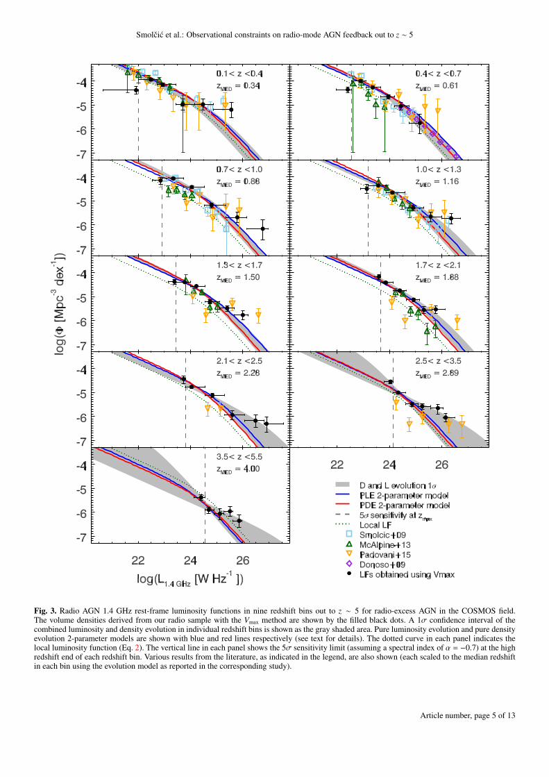
The 1.4 GHz radio luminosity functions (LFs) for our radioAGN, separated into 9 redshift ranges out to z ∼ 5, are shownin Fig. 3, and tabulated in Tab. 1. Redshift bins were chosen tobe large enough to contain a statistically significant number of

Article number, page 3 of 13

A&A proofs: manuscript no. ms_2c

Fig. 2. Spectral indices of our radio-excess AGN sample as a functionof redshift (grey points). Median values with interquartile ranges forsources with measured 1.4-3 GHz spectral indices in different redshiftbins are shown with blue circles. Mean values for all sources (i.e. alsoundetected at 1.4 GHz for which we manually set α = −0.7) in sameredshift bins are shown with red squares.

galaxies and to mitigate possible photometric uncertainties (i.e.sources falling into the wrong bin). We report LFs using the me-dian luminosity in each luminosity bin, while the error bars showthe width of the luminosity bin.

3.2. The evolution of the radio AGN luminosity function

The cosmic evolution of an astrophysical population is usuallyparameterized by density and luminosity evolution of its localluminosity function as:

Φ(L, z) = (1 + z)αD × Φ0

[

L

(1 + z)αL

]

, (1)

where αD and αL are the characteristic density and luminosityevolution parameters, respectively, L is the luminosity, Φ(L, z)is the luminosity function at redshift z, and Φ0 is the local lu-minosity function. The analytic form for the local radio AGNLF, adopted here, and also shown in Fig. 3, is taken fromMauch & Sadler (2007), and parametrized with two power-laws

Φ0(L) =Φ∗

(L∗/L)α + (L∗/L)β, (2)

where the parameters are the normalization Φ∗

=1

0.4 10−5.5 Mpc−3 dex−1 (scaled to the base of d log L), theknee position L∗ = 1024.59 W Hz−1, and the bright and faint endslopes α = −1.27, and β = −0.49, respectively. Mauch & Sadler(2007) derived their AGN LF using 2661 detections in the6dFGS–NVSS field with a median redshift of med(z) = 0.073and a span of six decades in luminosities. With such a samplethey were able to constrain well both the faint and the bright endof the local AGN LF.

In Fig. 4 we show the best fit pure density (PDE; αL = 0)and pure luminosity (PLE; αD = 0) evolutions for each redshiftbin (also tabulated in Tab. 2), which can be considered as the twoextreme cases of evolution. We note that the lowest luminositybin of our LFs is an outlier below z = 1.7, because of a com-bined effect of the flux sensitivity limit steeply rising within theredshift bin (see the red line in Fig. 1), and the radio AGN occu-pying the higher luminosity end within that redshift bin, causing

poorer sampling of the lowest luminosities inside any single red-shift range (with a median number of 19 sources in the lowestluminosity bins for z < 1.7; see Tab. 1, c.f., Tab. 1 in Novak et al.2017). These outliers were ignored in the fitting process.

To fit a simple, continuous model to the data, we followNovak et al. (2017), and add a redshift dependent term to theαL, and αD parameters in Eq. 1, and model the evolution of thelocal luminosity function using the following form:

Φ(L, z, αL, βL, αD, βD) = (1 + z)αD+z·βD ×Φ0

[

L

(1 + z)αL+z·βL

]

, (3)

where αL, βL, αD, and βD are the four free parameters. For pureluminosity evolution (αD = βD = 0) the χ2 minimization proce-dure yields best-fit parameter values of αL = 2.88 ± 0.82, βL =

−0.84 ± 0.34, while for pure density evolution (αL = βL = 0)the best-fit parameters are αD = 2.00± 0.18, βD = −0.60± 0.14.Fitting for all four parameters simultaneously yields a strong de-generacy between the parameters, and mainly differs from thetwo 2-parameter fits at the high luminosity end in high redshiftbins (z > 2.1). As discussed in more detail in Sect. 5, the vol-ume densities in these particular bins are the most sensitive tothe assumption of a simple synchrotron power-law for the K-correction to rest-frame 1.4 GHz luminosity from the observed3 GHz flux density. Hence, as the typical AGN spectrum at ra-dio frequencies in deep surveys, such as the VLA-COSMOS 3GHz survey, to-date is not constrained, and further, given the de-generacies inherent to the 4-parameter fit, we hereafter adopt thesimple continuous 2-parameter models as a representation of theevolution of the VLA-COSMOS 3 GHz (radio-excess) AGN. Wealso note that simple, pure luminosity (density) evolution mod-els are commonly used in the literature (e.g., Sadler et al. 2007;Smolcic et al. 2009; Donoso et al. 2009; McAlpine et al. 2013;Padovani et al. 2015).

3.3. Cosmic evolution of the number and radio luminositydensities

In Fig. 5 we show the redshift evolution of the number and lu-minosity densities using our 2-parameter evolution models, aswell as the best-fit pure luminosity and density evolutions ineach redshift bin. The number density in a given redshift bin wasobtained by integrating the corresponding luminosity functionover the logarithm of luminosity,

∫

Φ(L1.4GHz) d(log L1.4GHz),and the luminosity density by integrating the product of lumi-nosity and volume density over the logarithm of luminosity, i.e.,∫

L1.4GHz × Φ(L1.4GHz) d(log L1.4GHz).The number density of our radio AGN increases by a fac-

tor of ∼ 2 − 3 from z = 0 to z ∼ 1.5, beyond which it decreases,reaching a number density equivalent to that in the local universeat z ∼ 3.5, and further decreasing beyond this redshift. The lu-minosity density shows a similar behaviour. It rises by a factorof ∼ 2 − 4 from z = 0 to z ∼ 1.5, beyond which it decreases, atz ∼ 5 reaching a value about an order of magnitude lower thanthe luminosity density derived at z = 0.

3.4. Comparison with the literature

Based on the 2SLAQ Luminous Red Galaxy Survey containing∼ 400 galaxies in a volume-limited sample at 0.4 < z < 0.7Sadler et al. (2007) have found that their radio AGN (L1.4GHz ≈

1024− 1027 W Hz−1) undergo significant evolution since z ∼

0.7, parametrized with a pure luminosity evolution parameter

Article number, page 4 of 13

Smolcic et al.: Observational constraints on radio-mode AGN feedback out to z ∼ 5

Fig. 3. Radio AGN 1.4 GHz rest-frame luminosity functions in nine redshift bins out to z ∼ 5 for radio-excess AGN in the COSMOS field.The volume densities derived from our radio sample with the Vmax method are shown by the filled black dots. A 1σ confidence interval of thecombined luminosity and density evolution in individual redshift bins is shown as the gray shaded area. Pure luminosity evolution and pure densityevolution 2-parameter models are shown with blue and red lines respectively (see text for details). The dotted curve in each panel indicates thelocal luminosity function (Eq. 2). The vertical line in each panel shows the 5σ sensitivity limit (assuming a spectral index of α = −0.7) at the highredshift end of each redshift bin. Various results from the literature, as indicated in the legend, are also shown (each scaled to the median redshiftin each bin using the evolution model as reported in the corresponding study).

Article number, page 5 of 13

A&A proofs: manuscript no. ms_2c

Table 1. Luminosity functions of radio-excess AGN obtained with the Vmax method.

Redshift log(

L1.4 GHz

W Hz−1

)

log

(

Φ

Mpc−3 dex−1

)

N

0.1 < z < 0.4 21.92+0.081−1.3 -4.38+0.16

−0.15 10

22.48+0.24−0.48 -3.94+0.067

−0.058 49

22.93+0.50−0.22 -4.15+0.083

−0.070 33

23.70+0.45−0.27 -4.97+0.25

−0.22 5

24.48+0.39−0.33 -4.97+0.25

−0.22 5

25.56+0.031−0.69 -5.19+0.34

−0.30 3

0.4 < z < 0.7 22.41+0.15−0.43 -4.36+0.13

−0.097 19

22.89+0.21−0.33 -3.99+0.047

−0.042 97

23.36+0.29−0.26 -4.26+0.061

−0.053 59

23.96+0.24−0.30 -4.65+0.097

−0.079 25

24.44+0.31−0.24 -5.05+0.16

−0.15 10

25.16+0.13−0.42 -5.75+0.45

−0.37 2

0.7 < z < 1.0 22.86+0.064−0.32 -4.15+0.17

−0.12 25

23.34+0.39−0.42 -4.07+0.035

−0.032 208

24.05+0.49−0.32 -4.42+0.059

−0.052 98

24.80+0.55−0.26 -5.19+0.11

−0.090 19

25.79+0.37−0.44 -5.69+0.22

−0.20 6

26.76+0.21−0.60 -6.17+0.45

−0.37 2

1.0 < z < 1.3 23.14+0.048−0.24 -4.50+0.18

−0.17 8

23.57+0.31−0.39 -4.36+0.043

−0.039 114

24.11+0.48−0.22 -4.66+0.056

−0.049 69

24.91+0.39−0.32 -5.29+0.13

−0.097 16

25.57+0.43−0.27 -5.67+0.20

−0.19 7

26.36+0.35−0.35 -5.73+0.22

−0.20 6

1.3 < z < 1.7 23.39+0.063−0.23 -4.38+0.097

−0.080 30

23.78+0.23−0.33 -4.40+0.040

−0.037 132

24.22+0.33−0.22 -4.56+0.046

−0.042 101

24.74+0.36−0.19 -5.21+0.10

−0.082 24

25.40+0.26−0.29 -5.49+0.14

−0.11 13

26.00+0.21−0.34 -5.77+0.20

−0.19 7

Redshift log(

L1.4 GHz

W Hz−1

)

log

(

Φ

Mpc−3 dex−1

)

N

1.7 < z < 2.1 23.60+0.060−0.17 -4.17+0.13

−0.098 30

23.86+0.29−0.20 -4.41+0.045

−0.041 106

24.39+0.25−0.24 -4.75+0.061

−0.054 60

24.92+0.22−0.28 -5.13+0.091

−0.075 28

25.32+0.31−0.18 -5.56+0.16

−0.15 10

25.77+0.35−0.14 -5.53+0.16

−0.15 10

2.1 < z < 2.5 23.74+0.091−0.10 -4.44+0.18

−0.13 13

24.04+0.53−0.21 -4.77+0.055

−0.049 74

24.84+0.48−0.27 -5.12+0.082

−0.069 37

25.60+0.46−0.29 -5.94+0.20

−0.19 7

26.48+0.32−0.43 -6.18+0.28

−0.25 4

26.90+0.64−0.11 -6.31+0.34

−0.30 3

2.5 < z < 3.5 24.04+0.11−0.24 -4.55+0.090

−0.075 53

24.33+0.29−0.18 -5.01+0.057

−0.051 67

24.86+0.23−0.24 -5.49+0.097

−0.079 26

25.25+0.32−0.16 -5.58+0.14

−0.10 18

25.85+0.19−0.28 -5.66+0.26

−0.16 13

26.14+0.37−0.10 -6.05+0.18

−0.17 8

3.5 < z < 5.5 24.41+0.16−0.28 -5.39+0.13

−0.10 18

24.70+0.21−0.14 -5.90+0.16

−0.11 11

25.12+0.14−0.21 -6.07+0.25

−0.22 5

25.51+0.10−0.25 -5.97+0.22

−0.20 6

25.86+0.10−0.25 -6.36+0.28

−0.25 4

αL = 2.0 ± 0.3. Donoso et al. (2009) found fully consistent re-sults, but with considerably smaller error bars as they used asample of over 14,000 radio AGN. These derivations are in verygood agreement with the luminosity function derived here (see0.4 < z < 0.7 bin in Fig. 3), as well as with the pure luminos-ity evolution we find for the VLA-COSMOS radio-excess AGN,detected at 3 GHz (see top panel of Fig. 4).

McAlpine et al. (2013) studied the evolution of faint radioAGN in the VIDEO-XMM3 field out to z ∼ 2.5. By fitting a com-bined evolution of star forming and AGN galaxies, they founda slightly weaker evolution than that inferred by Sadler et al.

(2007, see Table 4 in McAlpine et al. 2013). The authors arguethat this is due to the fact that the evolution of the VIDEO-XMM3 radio AGN is primarily driven by the higher redshiftrange (0.9 < z < 2.5), not constrained by the 2SLAQ sur-vey. The pure luminosity evolution inferred by McAlpine et al.(2013, αL = 1.2 ± 0.2) is consistent with the average αL de-rived here in the equivalent (0.9 < z < 2.5) redshift range (forexample, for z = 1.75, αL + z · βL = 1.4 ± 1.0 for our pure lumi-nosity 2-parameter fit; see top panel of Fig. 4). In each redshiftrange the VIDEO-XMM3-based volume densitites of their AGN(shown in Fig. 3), identified during the photometric-redshift es-

Article number, page 6 of 13

Smolcic et al.: Observational constraints on radio-mode AGN feedback out to z ∼ 5

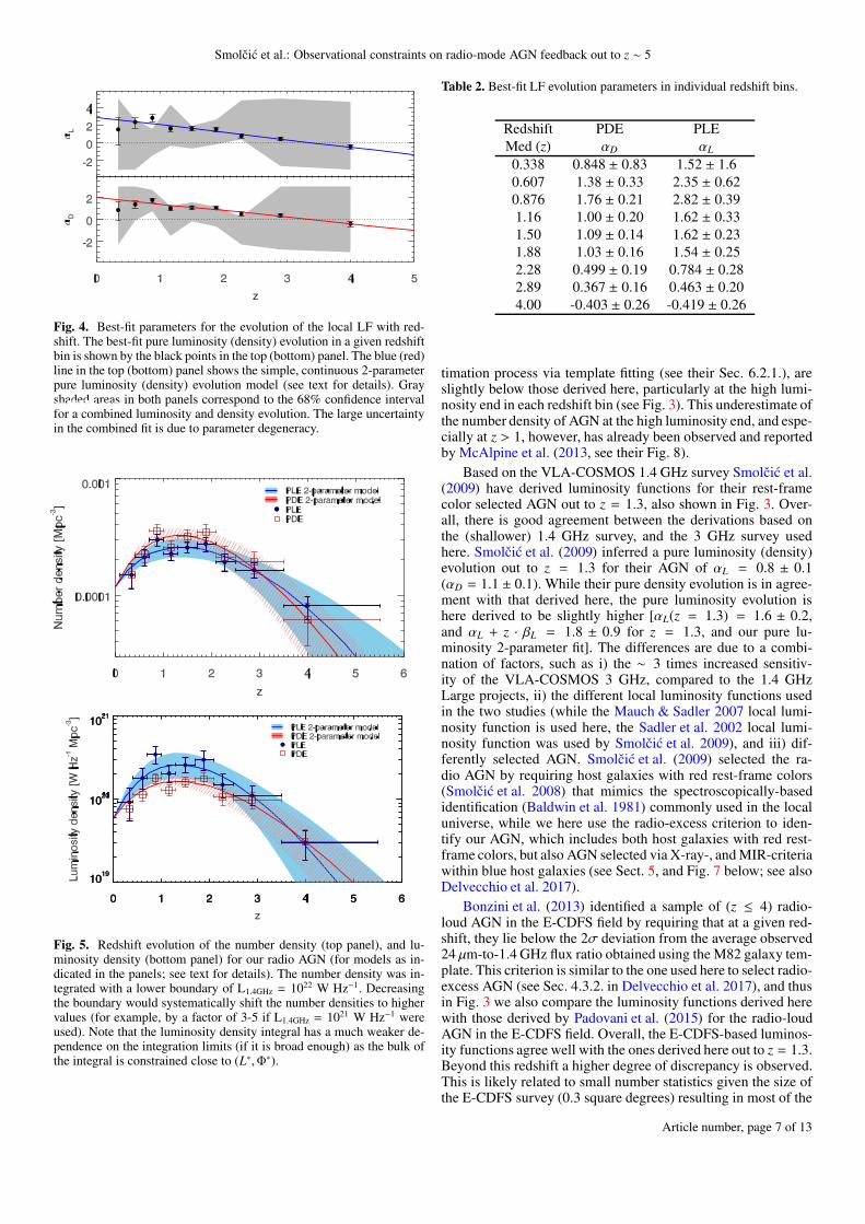
Fig. 4. Best-fit parameters for the evolution of the local LF with red-shift. The best-fit pure luminosity (density) evolution in a given redshiftbin is shown by the black points in the top (bottom) panel. The blue (red)line in the top (bottom) panel shows the simple, continuous 2-parameterpure luminosity (density) evolution model (see text for details). Grayshaded areas in both panels correspond to the 68% confidence intervalfor a combined luminosity and density evolution. The large uncertaintyin the combined fit is due to parameter degeneracy.

Fig. 5. Redshift evolution of the number density (top panel), and lu-minosity density (bottom panel) for our radio AGN (for models as in-dicated in the panels; see text for details). The number density was in-tegrated with a lower boundary of L1.4GHz = 1022 W Hz−1. Decreasingthe boundary would systematically shift the number densities to highervalues (for example, by a factor of 3-5 if L1.4GHz = 1021 W Hz−1 wereused). Note that the luminosity density integral has a much weaker de-pendence on the integration limits (if it is broad enough) as the bulk ofthe integral is constrained close to (L∗,Φ∗).

Table 2. Best-fit LF evolution parameters in individual redshift bins.

Redshift PDE PLEMed (z) αD αL

0.338 0.848 ± 0.83 1.52 ± 1.60.607 1.38 ± 0.33 2.35 ± 0.620.876 1.76 ± 0.21 2.82 ± 0.391.16 1.00 ± 0.20 1.62 ± 0.331.50 1.09 ± 0.14 1.62 ± 0.231.88 1.03 ± 0.16 1.54 ± 0.252.28 0.499 ± 0.19 0.784 ± 0.282.89 0.367 ± 0.16 0.463 ± 0.204.00 -0.403 ± 0.26 -0.419 ± 0.26

timation process via template fitting (see their Sec. 6.2.1.), areslightly below those derived here, particularly at the high lumi-nosity end in each redshift bin (see Fig. 3). This underestimate ofthe number density of AGN at the high luminosity end, and espe-cially at z > 1, however, has already been observed and reportedby McAlpine et al. (2013, see their Fig. 8).

Based on the VLA-COSMOS 1.4 GHz survey Smolcic et al.(2009) have derived luminosity functions for their rest-framecolor selected AGN out to z = 1.3, also shown in Fig. 3. Over-all, there is good agreement between the derivations based onthe (shallower) 1.4 GHz survey, and the 3 GHz survey usedhere. Smolcic et al. (2009) inferred a pure luminosity (density)evolution out to z = 1.3 for their AGN of αL = 0.8 ± 0.1(αD = 1.1 ± 0.1). While their pure density evolution is in agree-ment with that derived here, the pure luminosity evolution ishere derived to be slightly higher [αL(z = 1.3) = 1.6 ± 0.2,and αL + z · βL = 1.8 ± 0.9 for z = 1.3, and our pure lu-minosity 2-parameter fit]. The differences are due to a combi-nation of factors, such as i) the ∼ 3 times increased sensitiv-ity of the VLA-COSMOS 3 GHz, compared to the 1.4 GHzLarge projects, ii) the different local luminosity functions usedin the two studies (while the Mauch & Sadler 2007 local lumi-nosity function is used here, the Sadler et al. 2002 local lumi-nosity function was used by Smolcic et al. 2009), and iii) dif-ferently selected AGN. Smolcic et al. (2009) selected the ra-dio AGN by requiring host galaxies with red rest-frame colors(Smolcic et al. 2008) that mimics the spectroscopically-basedidentification (Baldwin et al. 1981) commonly used in the localuniverse, while we here use the radio-excess criterion to iden-tify our AGN, which includes both host galaxies with red rest-frame colors, but also AGN selected via X-ray-, and MIR-criteriawithin blue host galaxies (see Sect. 5, and Fig. 7 below; see alsoDelvecchio et al. 2017).

Bonzini et al. (2013) identified a sample of (z ≤ 4) radio-loud AGN in the E-CDFS field by requiring that at a given red-shift, they lie below the 2σ deviation from the average observed24 µm-to-1.4 GHz flux ratio obtained using the M82 galaxy tem-plate. This criterion is similar to the one used here to select radio-excess AGN (see Sec. 4.3.2. in Delvecchio et al. 2017), and thusin Fig. 3 we also compare the luminosity functions derived herewith those derived by Padovani et al. (2015) for the radio-loudAGN in the E-CDFS field. Overall, the E-CDFS-based luminos-ity functions agree well with the ones derived here out to z = 1.3.Beyond this redshift a higher degree of discrepancy is observed.This is likely related to small number statistics given the size ofthe E-CDFS survey (0.3 square degrees) resulting in most of the

Article number, page 7 of 13

A&A proofs: manuscript no. ms_2c

E-CDFS volume density values at z > 1.3 constrained by binscontaining fewer than 3 sources (c.f. Table 5 in Padovani et al.2015 and Tab. 1 here).

4. Radio-mode feedback considerations

In this Section we derive the cosmic evolution of the radio AGNkinetic luminosity density (Sect. 4.1), and compare it with theSAGE semi-analytic model (Sect. 4.2). We discuss various un-knowns from both the semi-analytic, and observational aspectsin Sect. 5.

4.1. Cosmic evolution of the radio AGN kinetic luminositydensity

The AGN studied here have, by construction, an observed excessof radio emission relative to that expected from star-formationprocesses within their host galaxies. Thus, the origin of the ob-served 3 GHz radio emission in these sources is related to theAGN itself, i.e. to the energy released through mass accretiononto the central SMBH. This energy can be efficiently radiatedaway and/or channeled in kinetic form via collimated jets ex-panding through and beyond the host galaxy, and observable atradio wavelengths. The observed radio emission in our sources(albeit mostly unresolved or barely resolved at 0.75′′ resolu-tion), can, thus, be predominantly attributed to the synchrotronemission of relativistic particles within the sources’ jet structures(i.e., core/jets/lobes). However, the observed radio emission willamount to only a fraction of the total kinetic luminosity2 of thejets, while a much larger fraction will be stored as the inter-nal energy of the jets/lobes, and lost to the environment via thework done by the expanding radio jets (e.g. Willott et al. 1999).The last is of particular interest as the energy (per unit time)deposited into the surroundings and dissipated can be directlylinked to the heating of the surrounding medium generated bythe jets of such AGN (see McNamara & Nulsen 2007, 2012 forreviews).

A simple scaling relation between the monochromatic ra-dio and kinetic luminosities has been long sought for. InAppendix A we give a detailed overview of such scal-ing relations, available in the literature (Willott et al. 1999;Bîrzan et al. 2004; Bîrzan et al. 2008; Merloni & Heinz 2007;Cavagnolo et al. 2010; O’Sullivan et al. 2011; Daly et al. 2012;Godfrey & Shabala 2016). We hereafter adopt the relation de-rived by Willott et al. (1999) at 151 MHz rest-frame fre-quency, and converted to 1.4 GHz rest-frame luminosity(Heckman & Best 2014), given as

log Lkin(LL1.4GHz) = 0.86 · log LL1.4GHz + 14.08 + 1.5 log fW, (4)

where Lkin is the kinetic luminosity in units of W, LL1.4GHz is the1.4 GHz rest-frame luminosity in units of W/Hz, and fW is anuncertainty parameter (see below).

Willott et al. (1999) estimated the kinetic energy using min-imum energy arguments, i.e. computing the minimum energystored in the lobes to produce the observed synchrotron luminos-ity, considering the age of the source and the efficiency of con-version of the kinetic luminosity into the internal energy of theobserved synchrotron emission. They have folded all uncertainty

2 The total kinetic luminosity is taken to equal the total energy trans-ported by the jets during the life-time of the radio source (Willott et al.1999).

factors in the calculation (such as departure from minimum en-ergy conditions, uncertainty in the energy in non-radiating par-ticles, and the composition of the jet) into one parameter, fW,estimated to lie in the range of fW ≈ 1 − 20. For fW = 15the normalization is close to that of the jet kinetic luminosi-ties computed through X-ray observations of galaxy clusterswith cavities induced in the hot, X-ray emitting instracluster gasby the radio jets/lobes (Bîrzan et al. 2004; Bîrzan et al. 2008;Merloni & Heinz 2007; Cavagnolo et al. 2010; O’Sullivan et al.2011), and for fW = 4 it matches the relation derived for pow-erful radio galaxies using equations of strong shock physics (seeDaly et al. 2012, and references therein). We, however, also con-sider the full range of the uncertainty parameter ( fW = 1 − 20;see below).

The kinetic luminosity density at a given redshift is com-puted as the integral of the kinetic luminosity density over (thelogarithm of the) monochromatic 1.4 GHz radio luminosity:

Ωkin(z) =∫

Lkin(LL1.4GHz) ×Φ(LL1.4GHz) d(log L1.4GHz). (5)

In Fig. 6 we show the cosmic evolution of the kinetic luminos-ity density, derived using our 2-parameter continuous evolutionmodel (Eq. 3), and the scaling relation between monochromaticradio luminosity and kinetic luminosity of Willott et al. (1999,Eq. 4) with uncertainty parameters fW = 4, and 15, as well as therange encompassed by the extreme values of fW (= 1, 20). Notethat the various fW values only systematically shift the derivedvolume-averaged kinetic luminosity density as a function of red-shift. Furthermore, the derivation for fW = 1 can be consideredas a robust lower limit, as any other scaling relation available inthe literature would have resulted in systematically higher values(see Appendix A for details). Under the assumptions made, thekinetic luminosity density rises by about a factor of three fromz = 0 to z ∼ 1.5, and decreases thereafter by close to two ordersof magnitude by z ∼ 5. This holds for both of our (pure luminos-ity and pure density) 2-parameter models, as also illustrated inFig. 6.

4.2. Comparison with the SAGE semi-analytic model

In Fig. 6 we compare the redshift evolution of the COSMOS ra-dio AGN kinetic luminosity density with that from the SAGEmodel (Croton et al. 2016). The SAGE model is a significant up-date of the semi-analytic model by Croton et al. (2006), includ-ing implementation of a more complex cycle between gas cool-ing and the radio-mode AGN heating. It is assumed that hot gasaccretes onto the central black hole following the Bondi-Hoyleaccretion (Bondi 1952), but including a, so-called, radio-modeefficiency parameter (κR; see Eq. 16 in Croton et al. 2016). Thisparameter is used to modulate the strength of black hole accre-tion (m), assumed to be related to the luminosity of the black holein radio mode in the standard way, as L = ηmc2, where η = 0.1is the standard efficiency of mass to energy conversion, and c isthe speed of light. In the SAGE model this luminosity is taken asthe source of heating that offsets the energy losses of the cool-ing gas, such that the heating rate is simply the ratio between theluminosity and the specific (per unit mass) energy of gas in thehot halo (see Eq. 17 and Sec. 9.1. in Croton et al. 2016). The ac-cretion luminosity assumed in the SAGE model can be taken asan equivalent to the, here derived, jet kinetic luminosity assum-ing that the bulk of the accretion energy is channelled in kinetic(rather than radiative) form. Hence, in Fig. 6 we can comparethe redshift evolution of the COSMOS radio AGN kinetic lu-minosity density with the volume-averaged accretion luminosity

Article number, page 8 of 13

Smolcic et al.: Observational constraints on radio-mode AGN feedback out to z ∼ 5

Fig. 6. Cosmic evolution of the kinetic luminosity density for our ra-dio AGN. The kinetic luminosity density was derived using Eq. 5, andthe Willott et al. (1999) relation between monochromatic (1.4 GHz rest-frame) radio luminosity and kinetic luminosity (Eq. 4) with fW = 4(pure luminosity evolution, PLE, model: blue full curve and blue shadedarea showing the 1σ uncertainty), fW = 15 (purple full curve, andpurple-hatched area showing the 1σ uncertainty), and fW = 1, and 20,with folded 1σ fitting errors (lower and upper gray dashed curves, re-spectively). Also shown is the kinetic luminosity density assumed inthe SAGE semi-analytic cosmological model (green dash-dotted curve;Croton et al. 2016). For comparison, the evolution of the kinetic lumi-nosity density for our radio AGN for the pure density evolution, PDE,model using only fW = 4 (Eq. A.1) is also shown with the red full curveand red-hatched area. To avoid overcrowding the panel the PDE resultfor fW = 15 is not shown, but note that it would be only systematicallyhigher compared to the fW = 4 PDE model result, and coincident withthat for PLE with the corresponding fW = 15 value. See also Fig. A.2for results based on other scaling relations.

responsible for radio-mode feedback in the SAGE model, whichis equivalent to that obtained by Croton et al. (2006, their Fig. 3),but scaled by the radio-mode efficiency parameter (κR = 0.08;see Sec. 9.1.1. in Croton et al. 2016).

As seen in Fig. 6 at z & 1 we find a remarkably similar slopeof the redshift evolution of the COSMOS radio AGN kinetic lu-minosity density and the radio-mode accretion luminosity usedin the SAGE model, with the absolute values of the same or-der for fW = 4 (the uncertainty parameter in the radio lumi-nosity – kinetic luminosity relation; Eq. 4). At z < 1 we find asteeper evolution than that in the SAGE model, with our z = 0value being a factor of 3-4 lower ( fW = 4). For fW = 15 the ki-netic luminosity density is at every redshift systematically higherthan the radio-mode accretion luminosity in the model, while forthe robust lower limit value ( fW = 1) the observationally basedkinetic luminosity density is at each redshift about an order ofmagnitude lower than that in the SAGE model. Overall, for themost likely values of the normalization of the radio luminos-ity – kinetic luminosity relation ( fW = 4, 15; see previous sec-tion, and Appendix A), the redshift evolution of the COSMOSradio AGN kinetic luminosity density is either on the same scaleas that in the model, or systematically higher by about an or-der of magnitude (or even higher if other scaling relations areused; see Fig. A.2). This would suggest that in both cases the en-ergy deposited by faint radio AGN into their environment maybe sufficient to offset the cooling energy losses, as postulatedin the model. However, there is still a non-negligible number ofsimplifications and unknowns inherent to both the semi-analyticmodels, and the observational results, as discussed in the nextsection.

5. Discussing the unknowns

Observational studies of radio-selected AGN find two radio-luminous AGN populations, with distinct host galaxy,and AGN properties (Smolcic 2009; Smolcic et al. 2009;Smolcic et al. 2015; Smolcic 2016; Hardcastle et al. 2007;Buttiglione et al. 2010; Heckman & Best 2014; Bonzini et al.2015; Padovani et al. 2015; Padovani 2016; Tadhunter 2016).One population is consistent with the standard, unified modelAGN picture, in which the accretion occurs in a radiativelyefficient manner, at high Eddington rates (1 − 10% . λEdd . 1).Evidence has been presented that this class is fuelled by the coldintra-galactic medium (IGM) phase, and that it is not too likelyto launch collimated jets (observable at radio wavelengths).The second population, however, exhibits radiatively inefficientaccretion related to low Eddington ratios (λEdd . 1 − 10%),and may be fuelled by the hot phase of the IGM. It has beenshown that this population is highly efficient in collimated jetproduction. The observed difference in Eddington ratio betweenthe two populations can be linked to the switch betweenthe standard accretion flow model, i.e., radiatively efficient,geometrically thin (but optically thick) disk accretion flows(Shakura & Sunyaev 1973), and a radiatively inefficient, geo-metrically thick (but optically thin) disk accretion flows (Esin1997; Narayan et al. 1998), occuring at accretion rates below acertain Eddington ratio (1-10%; Rees et al. 1982; Narayan & Yi1994; Meier 2002; Fanidakis et al. 2011). Further differenceshave been found demonstrating that the population of radiativelyefficient accretors dominates the radio-AGN number densititesat the bright end (e.g., L1.4GHz & 1026 W Hz−1for z < 0.3;Pracy et al. 2016), and that this population evolves more rapidlywith cosmic time (e.g. Willott et al. 2001; Pracy et al. 2016).

The radio AGN studied here have been selected based on anexcess of their radio emission relative to that expected from the(IR-based) star-formation rates in their host galaxies, thus as-suring that (& 80% of) the radio emission arises from the AGN(core/jet/lobe) component. To shed light onto which of the twoabove defined AGN classes our radio-excess AGN belong to, inFig. 7 we plot the absolute and fractional contributions of X-ray-, and MIR-selected AGN, as well as the remaining AGN (notidentified via X-ray or MIR emission), and hosted by red, quies-cent galaxies, and those hosted by galaxies with blue/green rest-frame colors implying substantial star formation activity in thehosts (see Smolcic et al. 2017a for details). The X-ray and MIRregimes provide an efficient approach to identify radiatively ef-ficient AGN, while red, quiescent host galaxies of radio AGNare shown to contain AGN with systematically lower radiativeAGN luminosities (see, e.g., Fig. 7 in Smolcic et al. 2017a), andfurther, this selection can be used to trace radiatively inefficientAGN (at least in the local universe; e.g., Smolcic 2009).

As seen in Fig. 7, at z . 1 our radio-excess AGN are com-posed of similar fractions of i) red, quiescent galaxies, and ii)X-ray, MIR, and those hosted by star-forming galaxies, but notidentified via X-ray or MIR emission. Beyond z = 1 the frac-tion of red, quiescent galaxies decreases steeply to a minimalfraction by z ∼ 2. Hence, we can conclude that AGN with obser-vational signatures of radiatively efficient accretion flows com-prise a non-negligible fraction of our radio-excess AGN (30-40% X-ray- and MIR-selected AGN). If only a fraction of theradio-excess AGN hosted by blue/green, star-forming galaxieswould also contain radiatively efficient AGN, which could bethe case given the expected cold gas supply in such, activelystar-forming galaxies (e.g. Vito et al. 2014), the fraction of ra-diatively efficient AGN in our radio-excess sample would rise

Article number, page 9 of 13

A&A proofs: manuscript no. ms_2c

even further. This implies that our radio-excess AGN are likelya mix of radiatively efficient and inefficient black hole accretionflows, shown in other studies to evolve differently with cosmictime (e.g. Willott et al. 2001; Best et al. 2014; Pracy et al. 2016).

The volume densities derived here for our radio AGN are, atthe high luminosity end in every redshift range, somewhat higherthan our best fit pure luminosity/density 2-parameter models (seeFig. 3). This could potentially be attributed to the rise given thefaster evolution of the high-luminosity radio AGN, consistentwith the radiatively efficient accretion flow population. However,these particular, high-luminosity bins at each redshift are themost sensitive to the assumption of a simple synchrotron power-law for the conversion from the observed 3 GHz flux density torest-frame 1.4 GHz luminosity. For example, assuming a spec-tral index of α = −0.7 for all our AGN (instead of using the ob-served value, if available, which steepens toward high redshift;see Fig. 2), this would have no effect on the low-luminosity vol-ume densities in the high-redshift bins, but the high-luminositybin values would decrease to be consistent with the pure lumi-nosity (density) 2-parameter models.

If the typical radio AGN spectrum were to steepen towardsthe high-frequency end (due to synchrotron energy losses; e.g.Miley 1980), as sampled by the observed frequency of 3 GHzat z > 2 (corresponding to rest-frame frequencies of > 9 GHz)then, for example, a broken power-law, rather than a simple, sin-gle power-law assumption would be more appropriate for theK-correction. On the other hand, in this case the simple, singlepower-law assumption of α = −0.7 could result in a more correct1.4 GHz rest-frame luminosity value, than the directly observedhigher spectral index values. Indeed, our 3 GHz fluxes on av-erage decrease towards higher redshift. Given the substantiallyshallower flux limit of the 1.4 GHz survey, this suggests a biasagainst sources with flat radio spectra, and, thus, supports a flat-ter (intrinsic) spectral index distribution than the one observed.Investigating this robustly requires further radio data, and will bethe subject of forthcoming studies.

Although our radio-excess AGN are likely a mix of ra-diatively efficient and inefficient black hole accretion flows,Delvecchio et al. (2017) have shown that the host galaxy prop-erties (stellar mass, rest-frame color, star formation rate) and ki-netic luminosity of these various subpopulations are compara-ble (see Figs. 8-11 in Delvecchio et al. 2017 for their low-to-moderate and moderate-to-high radiative luminosity AGN, i.e.,their ’MLAGN’, and ’HLAGN with radio-excess’ populations).Hence, it may be plausible to assume that, if heating due to ra-dio outflows indeed is occurring in these systems, it operates ina similar fashion in the various AGN within our sample, andcomparable to that postulated in the SAGE model. In the SAGEmodel it is taken that cooling flows develop in any halo withmass & 2.5 · 1011 M⊙, and further, that Bondi-Hoyle accretionof the hot (subdominant) component of the cooling gas, whichfills the space between the (dominant) cold cloud component,is responsible for the luminosity of the SMBH in radio-mode.Taking the stellar mass – halo mass relation of Behroozi et al.(2010) the halo mass threshold beyond which radio-mode feed-back occurs can be converted to a stellar mass of & 5 · 109 M⊙.The stellar masses of our radio AGN satisfy this criterion (seeFig. 1), and can, hence, be taken as a representative popula-tion of that assumed in the SAGE model to be responsibe forradio-mode feedback. In that respect, the similarity between thehere derived redshift evolution of the kinetic luminosity densityand that assumed in the SAGE semi-analytic model (at leat atz > 1) is astonishing. As a further step a more complex treat-ment of radio AGN in semi-analytic models, taking into account

Fig. 7. Absolute (top panel) and fractional (bottom panel) contributionof various subpopulations (as indicated in the bottom panel) to the fullradio-excess AGN sample (black curve) as a function of redshift.

the two dominant (thin and thick disk) accretion flows, as wellas the spins of SMBHs, would be desirable (e.g. Fanidakis et al.2011). However, from an observational perspective likely thelargest source of uncertainty in studies of radio-mode feedbackis the uncertainty of the monochromatic radio luminosity to ki-netic luminosity conversion. The relation used here containes anuncertainty factor of the order of 20 ( fW in Eq. 4; Willott et al.1999), and various relations available in the literature are sum-marized in Appendix A. The kinetic luminosity has been demon-strated to be not only a function of monochromatic radio lu-minosity, but also of other parameters such as the AGN’s syn-chrotron electron age, and its environment (Bîrzan et al. 2008;Hardcastle & Krause 2014; Kapinska et al. 2015). A better con-straint of the relation as a function of redshift, and other physicalparameters is still awaited. In this context, deep radio surveys,observed in a large enough range of radio frequency, allowing tocompute synchrotron ages, could provide an important step to-wards better understanding of the relevance of radio-mode AGNfeedback in massive galaxy formation.

6. Summary and conclusions

We have used a sample of 1,814 radio AGN selected fromthe VLA-COSMOS 3 GHz Large Project, and with NIR-detected (COSMOS2015 catalog) counterparts (with photomet-ric or spectroscopic redshifts). These were selected to do radioemission in (> 3σ) excess of that expected from their hosts’ (IR-based) star formation rates. Such a criterion assures that at least80% of their radio emission is due to the AGN component. Thesample reaches out to a redshift of z < 6, it comprises 1.4 GHzrest-frame radio luminosities in the range of 1022

−1027 W Hz−1,and their typical stellar masses are within ∼ 3×(1010

−1011) M⊙.Using the 1/Vmax method we have derived the luminosity

functions of the radio AGN out to z ∼ 5. We have furtherconstrained the evolution of this population using continuous

Article number, page 10 of 13

Smolcic et al.: Observational constraints on radio-mode AGN feedback out to z ∼ 5

models of pure density, and pure luminosity evolutions find-ing best-fit parameters of Φ∗ ∝ (1 + z)(2.00±0.18)−(0.60±0.14)z, andL∗ ∝ (1+z)(2.88±0.82)−(−0.82±0.34)z, respectively. We find a turn-overin number and luminosity densities of the population at z ≈ 1.5.

The 1.4 GHz luminosity was converted to kinetic luminos-ity using an analytically-motivated relation. Taking into accountthe full range of uncertainty, we have derived the cosmic evo-lution of the kinetic luminosity density provided by our AGN,which we compare to the radio-mode AGN feedback assumed inthe "Semi-Analytic Galaxy Evolution" (SAGE) model. We findthat the kinetic luminosity exerted by our radio AGN may behigh enough at each cosmic epoch since z ∼ 5 to balance theradiative cooling of the hot gas, as assumed in the model. How-ever, although our findings support the idea of radio-mode AGNfeedback as a cosmologically relevant process in massive galaxyformation, many simplifications in both the observational andsemi-analytic approaches still remain and need to be resolvedbefore robust conclusions can be reached.

Acknowledgement

This research was funded by the European Union’s SeventhFrame-work programs under grant agreements 333654 (CIG,’AGN feedback’). VS, MN, ID, LC acknowledge support fromthe European Union’s Seventh Frame-work program under grantagreement 337595 (ERC Starting Grant, ’CoSMass’). MB ac-knowledges support from the PRIN-INAF 2014. ES acknowl-edges funding from the European Research Council (ERC) un-der the European Union’s Horizon 2020 research and innovationprogramme (grant agreement n 694343).

References

Allen, S. W., Dunn, R. J. H., Fabian, A. C., Taylor, G. B., & Reynolds, C. S.2006, MNRAS, 372, 21

An, T., & Baan, W. A. 2012, ApJ, 760, 77Baldwin, J. A., Phillips, M. M., & Terlevich, R. 1981, PASP, 93, 5Behroozi, P. S., Conroy, C., & Wechsler, R. H. 2010, ApJ, 717, 379Benson, A. J., Bower, R. G., Frenk, C. S., et al. 2003, ApJ, 599, 38Best, P. N., Kaiser, C. R., Heckman, T. M., & Kauffmann, G. 2006, MNRAS,

368, L67Best, P. N., Kauffmann, G., Heckman, T. M., & Ivezic, Ž. 2005, MNRAS, 362,

9Best, P. N., Ker, L. M., Simpson, C., Rigby, E. E., & Sabater, J. 2014, MNRAS,

445, 955Bîrzan, L., McNamara, B. R., Nulsen, P. E. J., Carilli, C. L., & Wise, M. W. 2008,

ApJ, 686, 859Bîrzan, L., Rafferty, D. A., McNamara, B. R., Wise, M. W., & Nulsen, P. E. J.

2004, ApJ, 607, 800Bondi, H. 1952, MNRAS, 112, 195Bonzini, M., Padovani, P., Mainieri, V., et al. 2013, MNRAS, 436, 3759Bonzini, M., Mainieri, V., Padovani, P., et al. 2015, MNRAS, 453, 1079Bower, R. G., Benson, A. J., Malbon, R., et al. 2006, MNRAS, 370, 645Brusa, M., Comastri, A., Gilli, R., et al. 2009, ApJ, 693, 8Buttiglione, S., Capetti, A., Celotti, A., et al. 2010, A&A, 509, A6Capak, P., Aussel, H., Ajiki, M., et al. 2007, ApJS, 172, 99Cattaneo, A., & Best, P. N. 2009, MNRAS, 395, 518Cavagnolo, K. W., McNamara, B. R., Nulsen, P. E. J., et al. 2010, ApJ, 720, 1066Chabrier, G. 2003, ApJ, 586, L133Clewley, L., & Jarvis, M. J. 2004, MNRAS, 352, 909Condon, J. J. 1992, ARA&A, 30, 575Croton, D. J., Springel, V., White, S. D. M., et al. 2006, MNRAS, 365, 11Croton, D. J., Stevens, A. R. H., Tonini, C., et al. 2016, ApJS, 222, 22Daly, R. A., Sprinkle, T. B., O’Dea, C. P., Kharb, P., & Baum, S. A. 2012, MN-

RAS, 423, 2498Delvecchio, I., Smolcic, V., Zamorani, G., et al. 2017, A&A, http://jvla-

cosmos.phy.hr/papers_dr1/Delvecchio_et_al.pdfDonoso, E., Best, P. N., & Kauffmann, G. 2009, MNRAS, 392, 617Dunlop, J. S., & Peacock, J. A. 1990, MNRAS, 247, 19Esin, A. A. 1997, ApJ, 482, 400Fabian, A. C. 2012, ArXiv e-prints, arXiv:1204.4114

Fanidakis, N., Baugh, C. M., Benson, A. J., et al. 2011, MNRAS, 410, 53Godfrey, L. E. H., & Shabala, S. S. 2016, MNRAS, 456, 1172Hardcastle, M. J., Evans, D. A., & Croston, J. H. 2007, MNRAS, 376, 1849Hardcastle, M. J., & Krause, M. G. H. 2014, MNRAS, 443, 1482Heckman, T. M., & Best, P. N. 2014, ARA&A, 52, 589Kapinska, A. D., Hardcastle, M., Jackson, C., et al. 2015, Advancing Astro-

physics with the Square Kilometre Array (AASKA14), 173Kauffmann, G., Heckman, T. M., & Best, P. N. 2008, MNRAS, 384, 953Kennicutt, Jr., R. C. 1998, ApJ, 498, 541Kimball, A. E., & Ivezic, Ž. 2008, AJ, 136, 684La Franca, F., Melini, G., & Fiore, F. 2010, ApJ, 718, 368Laigle, C., McCracken, H. J., Ilbert, O., et al. 2016, ApJS, 224, 24Mauch, T., & Sadler, E. M. 2007, MNRAS, 375, 931McAlpine, K., Jarvis, M. J., & Bonfield, D. G. 2013, MNRAS, 436, 1084McNamara, B. R., & Nulsen, P. E. J. 2007, ARA&A, 45, 117—. 2012, New Journal of Physics, 14, 055023Meier, D. L. 2002, New A Rev., 46, 247Merloni, A., & Heinz, S. 2007, MNRAS, 381, 589—. 2008, MNRAS, 388, 1011Miley, G. 1980, ARA&A, 18, 165Narayan, R., Mahadevan, R., Grindlay, J. E., Popham, R. G., & Gammie, C.

1998, ApJ, 492, 554Narayan, R., & Yi, I. 1994, ApJ, 428, L13Novak, M., Smolcic, V., Delhaize, J., et al. 2017, A&A, http://jvla-

cosmos.phy.hr/papers_dr1/Novak_et_al.pdfO’Sullivan, E., Giacintucci, S., David, L. P., et al. 2011, ApJ, 735, 11Padovani, P. 2016, A&A Rev., 24, 13Padovani, P., Bonzini, M., Kellermann, K. I., et al. 2015, ArXiv e-prints,

arXiv:1506.06554Pracy, M. B., Ching, J. H. Y., Sadler, E. M., et al. 2016, MNRAS, 460, 2Rafferty, D. A., McNamara, B. R., Nulsen, P. E. J., & Wise, M. W. 2006, ApJ,

652, 216Rees, M. J., Begelman, M. C., Blandford, R. D., & Phinney, E. S. 1982, Nature,

295, 17Rigby, E. E., Best, P. N., Brookes, M. H., et al. 2011, MNRAS, 416, 1900Sadler, E. M., Jackson, C. A., Cannon, R. D., et al. 2002, MNRAS, 329, 227Sadler, E. M., Cannon, R. D., Mauch, T., et al. 2007, MNRAS, 381, 211Sanders, D. B., Salvato, M., Aussel, H., et al. 2007, ApJS, 172, 86Schinnerer, E., Carilli, C. L., Scoville, N. Z., et al. 2004, AJ, 128, 1974Schinnerer, E., Smolcic, V., Carilli, C. L., et al. 2007, ApJS, 172, 46Schinnerer, E., Sargent, M. T., Bondi, M., et al. 2010, ApJS, 188, 384Schmidt, M., Schneider, D. P., & Gunn, J. E. 1995, AJ, 110, 68Scoville, N., Aussel, H., Brusa, M., et al. 2007, ApJS, 172, 1Shakura, N. I., & Sunyaev, R. A. 1973, A&A, 24, 337Sijacki, D., Springel, V., Di Matteo, T., & Hernquist, L. 2007, MNRAS, 380, 877Silverman, J. D., Green, P. J., Barkhouse, W. A., et al. 2008, ApJ, 679, 118Smolcic, V. 2016, in Active Galactic Nuclei: What’s in a Name?, 13Smolcic, V., Padovani, P., Delhaize, J., et al. 2015, Advancing Astrophysics with

the Square Kilometre Array (AASKA14), 69Smolcic, V. 2009, ApJ, 699, L43Smolcic, V., Delvecchio, I., Zamorani, G., et al. 2017a, A&A, http://jvla-

cosmos.phy.hr/papers_dr1/Smolcic_et_al_counterparts.pdfSmolcic, V., Novak, M., Bondi, M., et al. 2017b, A&A, http://jvla-

cosmos.phy.hr/papers_dr1/Smolcic_et_al_data.pdfSmolcic, V., Schinnerer, E., Scodeggio, M., et al. 2008, ApJS, 177, 14Smolcic, V., Zamorani, G., Schinnerer, E., et al. 2009, ApJ, arXiv:0901.3372Steinmetz, M. 1997, in The Early Universe with the VLT., ed. J. Bergeron, 156Tadhunter, C. 2016, A&A Rev., 24, 10Vito, F., Maiolino, R., Santini, P., et al. 2014, MNRAS, 441, 1059Waddington, I., Dunlop, J. S., Peacock, J. A., & Windhorst, R. A. 2001, MNRAS,

328, 882Willott, C. J., Rawlings, S., Blundell, K. M., & Lacy, M. 1999, MNRAS, 309,

1017Willott, C. J., Rawlings, S., Blundell, K. M., Lacy, M., & Eales, S. A. 2001,

MNRAS, 322, 536

Article number, page 11 of 13

A&A proofs: manuscript no. ms_2c

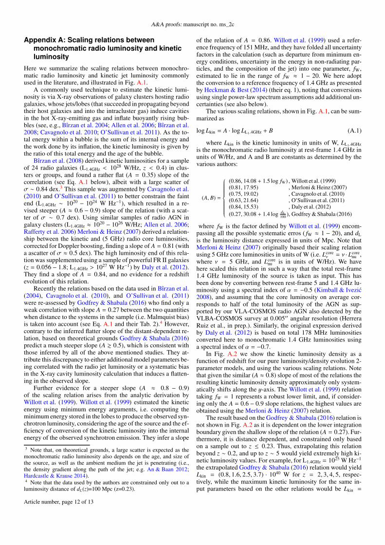
Appendix A: Scaling relations betweenmonochromatic radio luminosity and kineticluminosity

Here we summarize the scaling relations between monochro-matic radio luminosity and kinetic jet luminosity commonlyused in the literature, and illustrated in Fig. A.1.

A commonly used technique to estimate the kinetic lumi-nosity is via X-ray observations of galaxy clusters hosting radiogalaxies, whose jets/lobes (that succeeded in propagating beyondtheir host galaxies and into the intracluster gas) induce cavitiesin the hot X-ray-emitting gas and inflate buoyantly rising bub-bles (see, e.g., Bîrzan et al. 2004; Allen et al. 2006; Bîrzan et al.2008; Cavagnolo et al. 2010; O’Sullivan et al. 2011). As the to-tal energy within a bubble is the sum of its internal energy andthe work done by its inflation, the kinetic luminosity is given bythe ratio of this total energy and the age of the bubble.

Bîrzan et al. (2008) derived kinetic luminosities for a sampleof 24 radio galaxies (L1.4GHz < 1028 W/Hz, z < 0.4) in clus-ters or groups, and found a rather flat (A = 0.35) slope of thecorrelation (see Eq. A.1 below), albeit with a large scatter ofσ ∼ 0.84 dex.3 This sample was augmented by Cavagnolo et al.(2010) and O’Sullivan et al. (2011) to better constrain the faintend (L1.4GHz ∼ 1020

− 1024 W Hz−1), which resulted in a re-vised steeper (A ≈ 0.6 − 0.9) slope of the relation (with a scat-ter of σ ∼ 0.7 dex). Using similar samples of radio AGN ingalaxy clusters (L1.4GHz ≈ 1020

− 1026 W/Hz; Allen et al. 2006;Rafferty et al. 2006) Merloni & Heinz (2007) derived a relation-ship between the kinetic and (5 GHz) radio core luminosities,corrected for Doppler boosting, finding a slope of A = 0.81 (witha ascatter of σ ≈ 0.5 dex). The high luminosity end of this rela-tion was supplemented using a sample of powerful FR II galaxies(z = 0.056 − 1.8; L1.4GHz > 1027 W Hz−1) by Daly et al. (2012).They find a slope of A = 0.84, and no evidence for a redshiftevolution of this relation.

Recently the relations based on the data used in Bîrzan et al.(2004), Cavagnolo et al. (2010), and O’Sullivan et al. (2011)were re-assessed by Godfrey & Shabala (2016) who find only aweak correlation with slope A = 0.27 between the two quantitieswhen distance to the systems in the sample (i.e. Malmquist bias)is taken into account (see Eq. A.1 and their Tab. 2).4 However,contrary to the inferred flatter slope of the distant-dependent re-lation, based on theoretical grounds Godfrey & Shabala (2016)predict a much steeper slope (A & 0.5), which is consistent withthose inferred by all of the above mentioned studies. They at-tribute this discrepancy to either additional model parameters be-ing correlated with the radio jet luminosity or a systematic biasin the X-ray cavity luminosity calculation that induces a flatten-ing in the observed slope.

Further evidence for a steeper slope (A ≈ 0.8 − 0.9)of the scaling relation arises from the analytic derivation byWillott et al. (1999). Willott et al. (1999) estimated the kineticenergy using minimum energy arguments, i.e. computing theminimum energy stored in the lobes to produce the observed syn-chrotron luminosity, considering the age of the source and the ef-ficiency of conversion of the kinetic luminosity into the internalenergy of the observed synchrotron emission. They infer a slope

3 Note that, on theoretical grounds, a large scatter is expected as themonochromatic radio luminosity also depends on the age, and size ofthe source, as well as the ambient medium the jet is penetrating (i.e.,the density gradient along the path of the jet; e.g. An & Baan 2012;Hardcastle & Krause 2014).4 Note that the data used by the authors are constrained only out to aluminosity distance of dL(z)=100 Mpc (z=0.23).

of the relation of A = 0.86. Willott et al. (1999) used a refer-ence frequency of 151 MHz, and they have folded all uncertaintyfactors in the calculation (such as departure from minimum en-ergy conditions, uncertainty in the energy in non-radiating par-ticles, and the composition of the jet) into one parameter, fW,estimated to lie in the range of fW ≈ 1 − 20. We here adoptthe conversion to a reference frequency of 1.4 GHz as presentedby Heckman & Best (2014) (their eq. 1), noting that conversionsusing single power-law spectrum assumptions add additional un-certainties (see also below).

The various scaling relations, shown in Fig. A.1, can be sum-marized as

log Lkin = A · log LL1.4GHz + B (A.1)

where Lkin is the kinetic luminosity in units of W, LL1.4GHzis the monochromatic radio luminosity at rest-frame 1.4 GHz inunits of W/Hz, and A and B are constants as determined by thevarious authors:

(A, B) =

(0.86, 14.08 + 1.5 log fW) ,Willott et al. (1999)(0.81, 17.95) ,Merloni & Heinz (2007)(0.75, 19.02) , Cavagnolo et al. (2010)(0.63, 21.64) , O′Sullivan et al. (2011)(0.84, 15.53) , Daly et al. (2012)(0.27, 30.08 + 1.4 log dL

100 ), Godfrey & Shabala (2016)

where fW is the factor defined by Willott et al. (1999) encom-passing all the possible systematic erros ( fW ≈ 1 − 20), and dLis the luminosity distance expressed in units of Mpc. Note thatMerloni & Heinz (2007) originally based their scaling relationusing 5 GHz core luminosities in units of W (i.e. Lcore

ν = ν · Lcorenu ,

where ν = 5 GHz, and Lcorenu is in units of W/Hz). We have

here scaled this relation in such a way that the total rest-frame1.4 GHz luminosity of the source is taken as input. This hasbeen done by converting between rest-frame 5 and 1.4 GHz lu-minosity using a spectral index of α = −0.5 (Kimball & Ivezic2008), and assuming that the core luminosity on average cor-responds to half of the total luminosity of the AGN as sup-ported by our VLA-COSMOS radio AGN also detected by theVLBA-COSMOS survey at 0.005′′ angular resolution (HerreraRuiz et al., in prep.). Similarly, the original expression derivedby Daly et al. (2012) is based on total 178 MHz luminositiesconverted here to monochromatic 1.4 GHz luminosities usinga spectral index of α = −0.7.

In Fig. A.2 we show the kinetic luminosity density as afunction of redshift for our pure luminosity/density evolution 2-parameter models, and using the various scaling relations. Notethat given the similar (A ≈ 0.8) slope of most of the relations theresulting kinetic luminosity density approximately only system-atically shifts along the y-axis. The Willott et al. (1999) relationtaking fW = 1 represents a robust lower limit, and, if consider-ing only the A = 0.6 − 0.9 slope relations, the highest values areobtained using the Merloni & Heinz (2007) relation.

The result based on the Godfrey & Shabala (2016) relation isnot shown in Fig. A.2 as it is dependent on the lower integrationboundary given the shallow slope of the relation (A = 0.27). Fur-thermore, it is distance dependent, and constrained only basedon a sample out to z ≤ 0.23. Thus, extrapolating this relationbeyond z ∼ 0.2, and up to z ∼ 5 would yield extremely high ki-netic luminosity values. For example, for L1.4GHz = 1025 W Hz−1

the extrapolated Godfrey & Shabala (2016) relation would yieldLkin = (0.8, 1.6, 2.5, 3.7) · 1040 W for z = 2, 3, 4, 5, respec-tively, while the maximum kinetic luminosity for the same in-put parameters based on the other relations would be Lkin =

Article number, page 12 of 13

Smolcic et al.: Observational constraints on radio-mode AGN feedback out to z ∼ 5

Fig. A.1. Various scaling relations between monochromatic 1.4 GHz lu-minosity (L1.4GHz) and kinetic luminosity (Lkin) from the literature, as in-dicated in the top-left of the panel, and described in detail in the text (seeEq. A.1). Also shown, to guide the eye, are the data used by Bîrzan et al.(2004) and O’Sullivan et al. (2011) (L1.4GHz ≈ 1020

−1028 W Hz−1; filledsymbols). The analytically derived Willott et al. (1999) relation shownis that for fW = 15 (see text for details) in agreement with the relationsbased on a combination of X-ray cluster/group, and radio data (sym-bols). For fW = 4 it would agree with the Daly et al. (2012) relationinferred for powerful radio galaxies (L1.4GHz> 1027 W Hz−1).

1.6 ·1038 W (Merloni & Heinz 2007 relation), thus about two or-der of magnitude lower. We, however, note that out to z ∼ 0.1 theGodfrey & Shabala (2016) parametrization yields results consis-tent with the range of those obtained using the other relationsconsidered, and at z > 0.3 it results in kinetic luminosity den-sities increasingly higher by more than an order of magnitudecompared to the results based on the other relations.

Fig. A.2. The top (bottom) panel shows the kinetic luminosity densityas a function of redshift for our pure luminosity (density) evolution2-parameter model, using the various scaling relations commonly ap-plied in the literature, as indicated in each panel. For comparison theradio-model related SMBH accretion luminosity from the SAGE semi-analytic model (Croton et al. 2016) is also shown.

Article number, page 13 of 13