The wave geometry of final stratospheric warming eventsAmy H. Butler1 and Daniela I. V. Domeisen2
1Chemical Sciences Laboratory, National Oceanic and Atmospheric Administration, Boulder, CO, USA2Institute for Atmospheric and Climate Science, ETH Zürich, Zurich, Switzerland
Received: 23 December 2020 – Discussion started: 5 January 2021Revised: 21 April 2021 – Accepted: 29 April 2021 – Published: 27 May 2021
Abstract. Every spring, the stratospheric polar vortex tran-sitions from its westerly wintertime state to its easterly sum-mertime state due to seasonal changes in incoming solar ra-diation, an event known as the “final stratospheric warming”(FSW). While FSWs tend to be less abrupt than reversals ofthe boreal polar vortex in midwinter, known as sudden strato-spheric warming (SSW) events, their timing and characteris-tics can be significantly modulated by atmospheric planetary-scale waves. While SSWs are commonly classified accord-ing to their wave geometry, either by how the vortex evolves(whether the vortex displaces off the pole or splits into twovortices) or by the dominant wavenumber of the vortex justprior to the SSW (wave-1 vs. wave-2), little is known aboutthe wave geometry of FSW events. We here show that FSWevents for both hemispheres in most cases exhibit a clearwave geometry. Most FSWs can be classified into wave-1or wave-2 events, but wave-3 also plays a significant rolein both hemispheres. The timing and classification of theFSW are sensitive to which pressure level the FSW centraldate is defined, particularly in the Southern Hemisphere (SH)where trends in the FSW dates associated with ozone deple-tion and recovery are more evident at 50 than 10 hPa. How-ever, regardless of which FSW definition is selected, we findthe wave geometry of the FSW affects total column ozoneanomalies in both hemispheres and tropospheric circulationover North America. In the Southern Hemisphere, the timingof the FSW is strongly linked to both total column ozonebefore the event and the tropospheric circulation after theevent.
1 Introduction
The polar stratosphere exhibits a distinct seasonal cycle fea-turing a wintertime polar vortex, that is, strong circumpo-lar westerly winds that form in late summer and decay thefollowing spring, which is ultimately due to the seasonalcycle of incoming solar radiation. While the formation ofthe polar vortex occurs very predictably each year in latesummer of both hemispheres (late August in the NorthernHemisphere and mid-February in the Southern Hemisphere),the timing of the spring weakening of the vortex, the so-called final stratospheric warming (FSW) event, is more vari-able (Black et al., 2006; Black and McDaniel, 2007a). TheFSW marks the reversal of the climatological winter west-erlies to summer easterlies in the stratosphere, and its tim-ing varies by up to 2 months in the Northern Hemisphere(NH) and by more than 1 month in the Southern Hemi-sphere (SH) due to upward-propagating wave disturbancesfrom the troposphere that can disrupt the vortex ahead ofits radiatively driven decay (Waugh et al., 1999; Black andMcDaniel, 2007a, b). FSWs thus share many characteris-tics with dynamically driven midwinter disruptions of thepolar vortex, spectacular events called sudden stratosphericwarmings (SSWs; for a review see Baldwin et al., 2021),in which the polar stratosphere rapidly warms and the po-lar vortex winds reverse. However, FSW events are drivenby a combination of wave-induced and radiative processes(Salby and Callaghan, 2007) and thus occur every spring inboth hemispheres, while the occurrence of major SSW eventsis largely limited to the NH, with a notable exception in theSH spring of 2002 (e.g., Charlton et al., 2005). In the NH,SSWs on average occur about six times per decade (Charltonand Polvani, 2007) with strong decadal variability (Reichleret al., 2012; Domeisen, 2019). Further notable differences
Published by Copernicus Publications on behalf of the European Geosciences Union.
454 A. H. Butler and D. I. V. Domeisen: Final stratospheric warming geometry
between the NH and the SH include a longer lifespan of theSH vortex and a stronger distortion and displacement fromthe pole of the NH vortex (Waugh and Randel, 1999).
In the SH spring, the timing of the FSW is modulated byfeedbacks between chemical stratospheric ozone loss and thecirculation (Solomon et al., 2014). The SH spring vortex isclimatologically stronger and more stable compared to theNH, resulting in annual conditions ideal for the rapid destruc-tion of ozone by atmospheric chlorofluorocarbons, known asthe ozone hole (Solomon, 1999). As sunlight returns to thesouth pole every year in late September, a cascade of chemi-cal reactions rapidly destroys stratospheric ozone, which fur-ther cools and strengthens the polar vortex and allows thevortex to persist longer. The SH thus exhibits a long-termtrend in the timing of FSW events that is linked to ozonedepletion (e.g., Zhou et al., 2000; Haigh and Roscoe, 2009;Sheshadri et al., 2014). In the NH, where spring tempera-tures are rarely cold enough to support chemical reactionsfor rapid ozone loss, the persistence of the vortex in the NHspring is more closely linked to interannual variations in tro-pospheric wave forcing than to feedbacks with stratosphericozone (Chipperfield and Jones, 1999; Newman et al., 2001;Savenkova et al., 2012). Nevertheless certain boreal springs,as in 1997 and 2020, have been characterized by a persistentpolar vortex associated with extreme Arctic ozone loss (Coyet al., 1997; Lawrence et al., 2020). The timing of the FSW inboth hemispheres can have significant influence on the trans-port and mixing of stratospheric ozone (Rood and Schoeberl,1983; Manney and Lawrence, 2016). The presence of the po-lar vortex isolates polar stratospheric air, and so the seasonalbreakdown of the vortex allows for the sudden mixing andstirring of vortex air with ozone-rich midlatitude air. The tim-ing of the final warming modulates the strength and speed atwhich this mixing occurs (Waugh and Rong, 2002).
Just as for midwinter SSWs, changes in the stratosphereat the time of the final warming in spring can have an influ-ence on weather patterns in both hemispheres (Black et al.,2006; Black and McDaniel, 2007a), including extreme events(Domeisen and Butler, 2020). In the SH, the troposphericeddy-driven jet exhibits an equatorward shift at the time ofthe FSW related to a negative phase of the Southern AnnularMode (SAM) (Byrne et al., 2017; Byrne and Shepherd, 2018;Lim et al., 2018). The trend and variability in the timing ofthe FSW event due to ozone depletion has been suggestedto further affect the surface impact (Thompson et al., 2011;Son et al., 2013). In the Northern Hemisphere, the FSW isassociated with a weakening and equatorward shift of theNorth Atlantic storm track resembling the negative phase ofthe North Atlantic Oscillation (NAO), associated with highgeopotential height anomalies over the Arctic (Black et al.,2006; Ayarzagüena and Serrano, 2009). Consistent with thechemical-dynamic feedbacks discussed above, spring ozoneextremes have also been linked to anomalous surface weatherpatterns (Calvo et al., 2015; Ivy et al., 2017).
Furthermore, FSW events have been suggested to con-tribute to variability (Ayarzagüena and Serrano, 2009) andpredictability (Byrne et al., 2019; Hardiman et al., 2011;Butler et al., 2019) at the surface. While SSWs cannotbe predicted more than 1–2 weeks in advance (Taguchi,2014, 2016; Karpechko et al., 2018; Karpechko, 2018), FSWevents tend to be more predictable, especially events in latespring (Butler et al., 2019). The higher predictability of FSWevents with respect to SSW events may provide enhancedlead times for potential surface impacts in comparison toSSW events. For a comprehensive comparison of the pre-dictability timescales of sudden and final stratospheric warm-ing events, see Domeisen et al. (2020).
SSW events have been classified according to a range ofcharacteristics (Butler et al., 2015), notably with respect tothe zonal wavenumber dominating the polar stratosphere atthe time of or just prior to the event (Bancalá et al., 2012;Barriopedro and Calvo, 2014) or according to vortex ellipti-cal moment diagnostics (Waugh, 1997; Charlton and Polvani,2007; Mitchell et al., 2011; Seviour et al., 2013), that is,whether the vortex splits into two vortices or displaces offthe pole. They have also been classified with respect totheir downward impact (Kodera et al., 2016; Runde et al.,2016; Karpechko et al., 2017; Charlton-Perez et al., 2018;Domeisen, 2019; Afargan-Gerstman and Domeisen, 2020).FSW events, on the other hand, have generally been classi-fied according to the timing of their occurrence into “early”and “late” events (e.g., Waugh and Rong, 2002) and their al-titude of origin in the stratosphere (Hardiman et al., 2011).
Planetary wave activity from the troposphere to the strato-sphere is on average stronger in austral spring compared toaustral winter or boreal spring (Randel, 1988; Wang et al.,2019). Climatologically, in the SH late winter and springthe wave structure in the stratosphere is dominated by aquasi-stationary zonal wavenumber 1 (hereafter: wave-1)with contributions from a transient, eastward-moving zonalwavenumber 2 (hereafter: wave-2) (Randel, 1988; Mechosoet al., 1988; Manney et al., 1991; Waugh and Randel, 1999;Harvey et al., 2002; Ialongo et al., 2012), which may con-tribute to zonal asymmetries in ozone depletion (Kravchenkoet al., 2012). In the NH, early FSW events tend to be pre-dominantly wave-driven (e.g., Vargin et al., 2020). In fact,there is no mechanistic difference between midwinter SSWevents and early NH FSW events; they are merely differen-tiated through the evolution of the stratospheric winds afterthe event as the definition of the SSW requires the winds af-ter the event to return to westerly for a consecutive numberof days (Charlton and Polvani, 2007). Late FSWs may alsobe partly wave-driven, although as the mean flow weakens inboreal spring due to changing solar radiation, less weakeningby waves is required for an event to occur. Sun et al. (2011)show in a model study that FSW events tend to occur ear-lier if wave driving is increased, and a correspondence hasbeen found between the amplitude of wave-1 and the NHFSW date (Savenkova et al., 2012). Wave geometry can also
A. H. Butler and D. I. V. Domeisen: Final stratospheric warming geometry 455
be associated with the nonlinear resonance of the vortex, aprocess suggested to be potentially important in SH spring(Scott and Haynes, 2002; Plumb, 2010). Given the timingof FSW events in spring when the polar vortex has alreadyweakened, one could hypothesize that these events are moreoften caused by higher zonal wavenumbers (e.g., waves 2and 3) as compared to wave-1, as these will be allowed topropagate into the weaker winds (Charney and Drazin, 1961;Matsuno, 1970; Plumb, 1989). Nonetheless, a classificationof individual FSW events in the historical record based ongeometrical wave structure, and the influence of the wavegeometry on stratospheric ozone and surface impacts, doesnot yet exist.
This study explores the classification of FSW events bywave geometry (Sect. 2), the connections between wave ge-ometry and dynamical behavior in the stratosphere (Sect. 3),ozone distribution (Sect. 4), and surface impacts (Sect. 5).
2 Detection and classification of FSW events
Currently there exists no consistent metric for defining thecentral date of FSWs. While most metrics detect the FSWwhen springtime stratospheric zonal winds fall below a cer-tain threshold, different studies have considered multiplepressure levels (Hardiman et al., 2011), single pressure lev-els at varying latitudes and thresholds (Black and McDaniel,2007b; Byrne et al., 2017), or definitions along the locationof maximum potential vorticity gradient rather than a zonalmean (Waugh and Rong, 2002). In this study, we compareour results for metrics defined at two different pressure lev-els, 10 and 50 hPa. In particular, we define FSW dates inthese two ways:
1. FSW events are detected as the first date before 30 June(31 January) when the daily mean zonal-mean zonalwinds at 60◦ latitude and 10 hPa in the NH (SH) areeasterly and do not return to westerly for more than 10consecutive days (e.g., Butler and Gerber, 2018). An ad-vantage of this definition is that it is consistent with thedefinition of midwinter SSWs, which is based on the re-versal of the westerly winds at 10 hPa and 60◦ latitude(Charlton and Polvani, 2007), and can be used identi-cally in the NH and SH. The 10 hPa level is also optimalfor detecting dynamic changes in the polar stratosphere(Butler and Gerber, 2018).
2. FSW events are detected as the first date before 30 June(31 January) when the daily mean zonal-mean zonalwinds at 60◦ latitude and 50 hPa in the NH (SH) fallbelow 5 (10) ms−1 and do not return to westerly formore than 10 consecutive days (similar to Black andMcDaniel, 2007b, a). An advantage of this definition isthat the spring transition in the lower stratosphere maybetter reflect both chemistry–climate feedbacks associ-ated with trends in ozone and coupling to the surface.
Tables 1 and 2 list the calculated NH and SH FSW dates,respectively, using daily-mean data from JRA-55 reanaly-sis (Kobayashi et al., 2015) for the January 1958–December2019 period and for the definitions based at both 10 and50 hPa. We do not examine FSWs in the SH prior to 1979 be-cause large-scale dynamical features related to stratosphere–troposphere coupling processes are not reliable due to lackof assimilated observations in the SH prior to satellite mea-surements (Gerber and Martineau, 2018). We compare thesedates based on JRA-55 reanalysis to ERA-interim reanalysis(Dee et al., 2011) for the period in common between them,1979–2019; in general the dates are almost identical but canvary by 1–2 d.
We then classify FSW events by their geometry, eitherwave-1, wave-2, or wave-3, using the following method. Wefirst apply Fourier decomposition in the zonal direction ofthe 50 hPa geopotential heights averaged with cosine weight-ing by latitude over 55–65◦ latitude. The 50 hPa geopotentialheights are used for wave classification throughout, no matterthe level where the date of the FSW is defined, because wave-2 climatologically peaks at 50 hPa (Barriopedro and Calvo,2014; Gerber et al., 2021). We determine which wavenum-ber has, during the period 10 d prior to the FSW date, (1)the daily-mean maximum amplitude for the greatest numberof days and (2) the maximum mean amplitude averaged overthe 10 d period (similar to Bancalá et al., 2012, and Barriope-dro and Calvo, 2014, for midwinter SSWs). The former mea-sures the persistence, and the latter indicates the strength of agiven wavenumber; these different metrics frequently but notalways yield the same result (see Table A1).
For every event, each of these two metrics indicates a pref-erence for wave-1, wave-2, or wave-3. The final wave geome-try classification used throughout the remainder of this studyis then determined based on the agreement of these metrics.If they do not agree, the event is labeled as “unclassified”.Table A1 shows the individual classification for each metricfor JRA-55, as a demonstration of how the final classifica-tion was determined. For the period 1979–August 2019, wecheck the classifications using both ERA-interim and JRA-55 reanalysis data, as wave geometry for midwinter SSWshas been found to be sensitive to the reanalysis used (Gerberet al., 2021). In general, the classification of FSW events isconsistent across the two reanalysis products, although a fewdiscrepancies are noted in Tables 1 and 2.
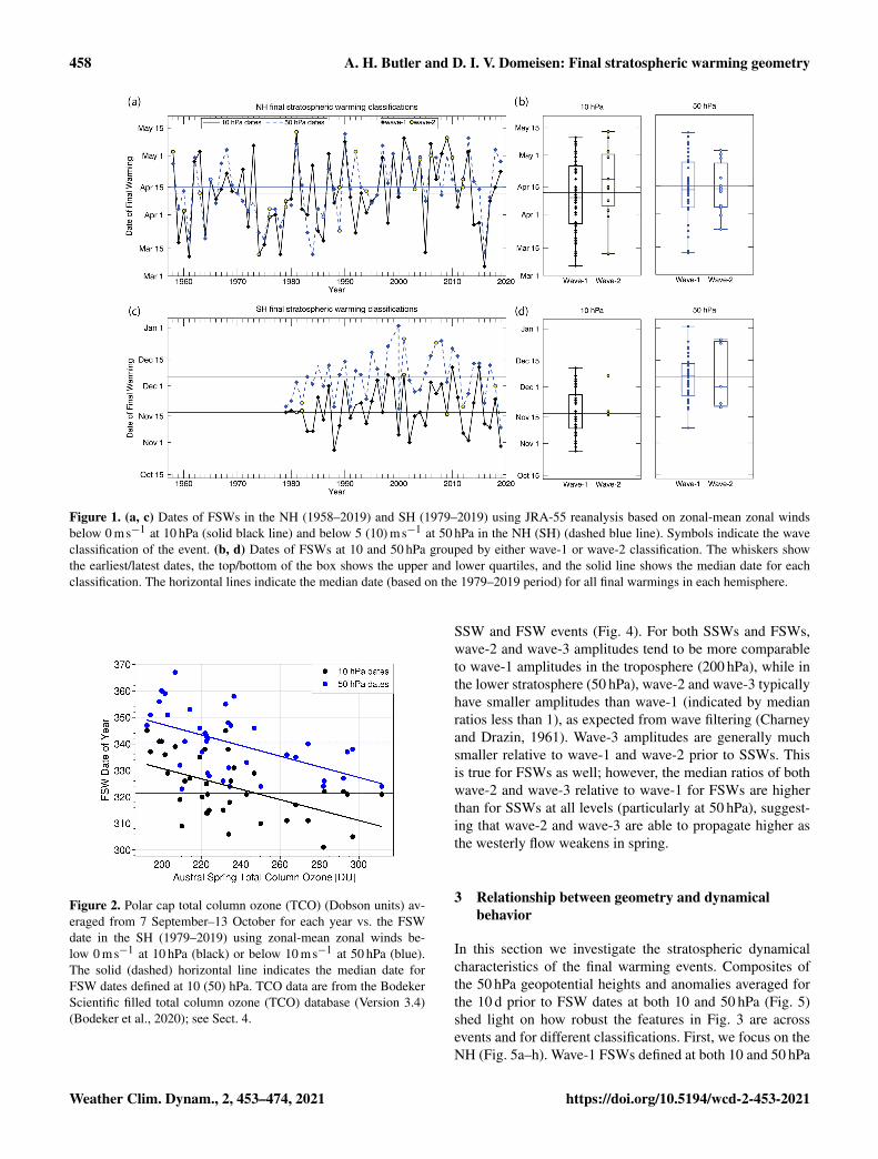
Figure 1a and c illustrates the sequence of dates of the fi-nal warmings at both 10 and 50 hPa along with their wavegeometry classification and their timing of occurrence withrespect to the median final warming date, indicated by hori-zontal lines. In this study we consider separately early events,those that occur more than 2 d prior to the median date, andlate events, those that occur more than 2 d after the mediandate. In the NH, the median date of the final warming basedon the 1979–2019 period is 12 April at 10 hPa and 15 Aprilat 50 hPa. In general there is little difference in the timingof the NH FSW for the 10 and 50 hPa metrics, though for a
456 A. H. Butler and D. I. V. Domeisen: Final stratospheric warming geometry
Table 1. Dates and classifications for FSW events in the Northern Hemisphere according to JRA-55 reanalysis. Early (late) events areindicated in bold (cursive), referring to a date before (after) the median date of 12 April at 10 hPa and 15 April at 50 hPa. Dates that fallwithin ±2 d of the median date are not classified as early or late. U= unclassified (methods did not agree according to the criterion outlinedin Sect. 2). Superscripts indicate the ERA-interim classification if it was not in agreement with JRA-55 during the 1979–2019 period.
Year Date Type Date Type Year Date Type Date Type10 hPa 50 hPa 10 hPa 50 hPa
1958 3 May wave-2 27 Apr wave-1 1989 15 Apr wave-2 24 Mar wave-2U
1959 18 Mar wave-1 4 Apr wave-1 1990 8 May wave-1 12 May wave-11960 2 Apr wave-2 12 Apr wave-1 1991 10 Apr wave-1 14 Apr wave-11961 11 Mar wave-1 20 Mar wave-1 1992 22 Mar wave-1 2 May wave-21962 28 Apr wave-1 30 Apr wave-1 1993 12 Apr wave-1 15 Apr wave-11963 3 May wave-1 12 Apr wave-2 1994 2 Apr wave-1 13 Apr wave-21964 19 Mar wave-1 19 Mar wave-1 1995 8 Apr wave-1 7 Apr wave-11965 19 Apr wave-2 19 Apr wave-2 1996 10 Apr wave-1 10 Apr wave-11966 9 Apr wave-1 7 Apr wave-1 1997 30 Apr wave-1 6 May wave-11967 14 Apr wave-1 27 Apr wave-1 1998 28 Mar wave-1 17 Apr wave-11968 21 Apr wave-1 3 May wave-1 1999 2 May wave-1 2 May wave-11969 13 Apr wave-1 16 Apr wave-1 2000 9 Apr wave-1 11 Apr wave-11970 12 Apr wave-1 12 Apr wave-1 2001 10 May wave-1 28 Apr U1971 24 Apr wave-1 8 Apr wave-1 2002 2 May U2 30 Apr wave-11972 25 Mar wave-1 2 Apr wave-1 2003 14 Apr wave-2 14 Apr wave-21973 6 May wave-1 8 Apr U 2004 29 Apr wave-2 28 Apr wave-21974 12 Mar wave-2 23 Mar wave-1 2005 13 Mar wave-1 8 Apr wave-11975 17 Mar wave-1 20 Mar wave-1 2006 7 May wave-1 1 May wave-21976 30 Mar wave-2 3 Apr wave-2 2007 19 Apr wave-1 30 Apr wave-11977 1 Apr wave-1 4 Apr wave-1 2008 1 May wave-1 10 Apr wave-11978 12 Mar wave-1 26 Mar wave-1 2009 10 May wave-2 1 May wave-31979 8 Apr wave-2 5 Apr wave-2 2010 30 Apr wave-2 19 Apr wave-11980 8 Apr wave-1 5 Apr wave-1 2011 5 Apr wave-1 13 Apr wave-11981 13 May wave-2 7 May wave-1 2012 18 Apr wave-2 14 Apr wave-21982 4 Apr wave-1 16 Apr wave-1 2013 3 May wave-1 10 May wave-1U
1983 1 Apr wave-1 23 Mar wave-1 2014 27 Mar wave-1 18 Apr wave-11984 25 Apr wave-1 11 Mar wave-1 2015 28 Mar wave-1 14 Apr wave-11985 24 Mar wave-1 4 Apr wave-1 2016 5 Mar wave-1 12 Mar wave-11986 19 Mar wave-1 31 Mar wave-2 2017 8 Apr wave-1 10 Apr wave-11987 2 May wave-1 24 Apr wave-1 2018 15 Apr wave-1U 4 May wave-11988 6 Apr wave-1 13 Apr wave-1 2019 23 Apr wave-1 28 Apr wave-1
few years they differ by more than a week. In the SH, themedian date of the final warming is 17 November at 10 hPaand 6 December at 50 hPa. Given the different classificationsfor FSW events in the literature, it is important to note thatdetecting the FSW at 10 or 50 hPa yields a much more sig-nificant shift in the timing of the SH as compared to the NH(Newman, 1986). In addition, for the 50 hPa dates in the SH,there is a clear trend towards later FSWs from 1979–2000,and a trend towards earlier FSWs from 2000–2019. While theformer has been previously linked to chemical ozone deple-tion (Waugh et al., 1999), the latter is an indicator of ozonerecovery which has recently been tied to a reversal in SH tro-pospheric circulation trends (Banerjee, Antara et al., 2020).These trends are less apparent for the 10 hPa dates. The lin-ear trend for the 1979–2000 period for the 50 hPa dates is+0.7± 0.4 dyr−1, whereas for the 10 hPa dates the trend is+0.5± 0.4 dyr−1 (both are significant, but the 10 hPa trend
is weaker). Similarly, the linear trend for the 2001–2019 pe-riod for the 50 hPa dates is −0.9± 0.5 dyr−1, whereas forthe 10 hPa dates the trend is not statistically significant at−0.4± 0.6 dyr−1.
Nonetheless, the interannual variability in the dates at 10and 50 hPa is strongly correlated in both hemispheres, atr = 0.68 (n= 62, ρ < 0.01) in the NH and r = 0.76 (n= 41,ρ < 0.01) in the SH. The FSW dates are more variable in theNH compared to the SH; the standard deviations are 18 (15) dfor the 10 (50) hPa classification in the NH (1958–2019) and12 d at both levels for the SH (1979–2019). In the NH, thetiming of FSWs has been linked to the occurrence of mid-winter SSWs, which are followed by a period of recovery towesterlies and thus later-than-normal FSWs (Hu et al., 2014).For example for the FSWs at 10 hPa, the median date foryears without midwinter SSWs is 1 April, whereas for yearswith SSWs the FSW date is 24 April. This difference reduces
A. H. Butler and D. I. V. Domeisen: Final stratospheric warming geometry 457
Table 2. Dates and classifications for FSW events in the Southern Hemisphere according to JRA-55 reanalysis. Early (late) events areindicated in bold (cursive), referring to a date before (after) the median date of 17 November at 10 hPa and 6 December at 50 hPa. Datesthat fall within ±2 d of the median date are not classified as early or late. U= unclassified (methods did not agree according to the criterionoutlined in Sect. 2). Superscripts indicate the ERA-interim classification if it was not in agreement with JRA-55 during the 1979–2018 period.
Year Date Type Date Type Year Date Type Date Type10 hPa 50 hPa 10 hPa 50 hPa
1979 17 Nov wave-1 20 Nov wave-1 2000 4 Nov wave-1 18 Nov wave-11980 17 Nov wave-1 22 Nov wave-1 2001 7 Dec wave-2 26 Dec wave-21981 17 Nov wave-2 3 Dec wave-1 2002 1 Nov wave-1 4 Dec wave-11982 18 Nov wave-2 22 Nov wave-2 2003 15 Nov wave-1 28 Nov wave-11983 7 Nov wave-1 6 Dec wave-1 2004 16 Nov wave-1 28 Nov wave-11984 6 Nov wave-1 1 Dec wave-1 2005 10 Nov wave-1 8 Dec wave-11985 25 Nov wave-1 12 Dec U1 2006 3 Dec wave-1 17 Dec wave-11986 13 Nov wave-1 1 Dec wave-1 2007 27 Nov wave-1 24 Dec wave-21987 1 Dec wave-1 12 Dec wave-1 2008 1 Dec wave-1 24 Dec wave-11988 27 Oct wave-1 19 Nov wave-1 2009 16 Nov wave-2 3 Dec wave-11989 10 Nov wave-1 7 Dec wave-1 2010 11 Dec wave-1 21 Dec wave-11990 4 Dec U1 14 Dec wave-1 2011 25 Nov wave-1 17 Dec wave-11991 14 Nov wave-1 20 Nov wave-1 2012 5 Nov wave-1U 19 Nov wave-21992 20 Nov U 8 Dec wave-1 2013 2 Nov wave-1 27 Nov wave-11993 22 Nov wave-1 7 Dec wave-1 2014 22 Nov wave-1 13 Dec wave-11994 11 Nov wave-1 24 Nov wave-1 2015 11 Dec wave-1 13 Dec wave-11995 23 Nov wave-1 19 Dec wave-1 2016 10 Nov wave-1 21 Nov wave-11996 3 Dec wave-1 9 Dec wave-1 2017 9 Nov wave-1 12 Dec wave-11997 17 Nov wave-1 25 Nov U 2018 24 Nov wave-1 1 Dec wave-21998 7 Dec wave-1U 22 Dec wave-1 2019 30 Oct wave-1 9 Nov wave-11999 5 Dec wave-1 2 Jan (2000) wave-1
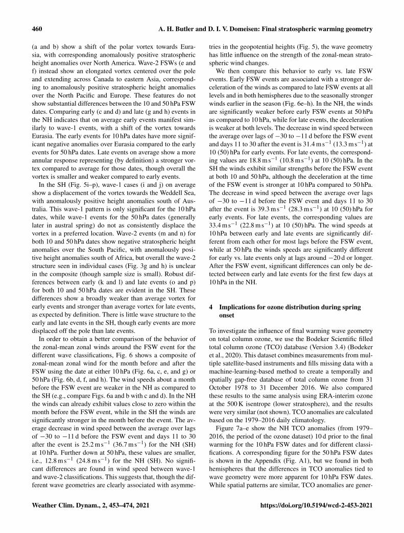
to 4 d for NH FSWs defined at 50 hPa. In the SH, years withlarger ozone loss in early austral spring lead via chemistry–climate feedbacks to a colder and more persistent polar vor-tex and later than average FSWs (Fig. 2; see also Zhang et al.,2017). This interannual relationship holds for both 10 and50 hPa dates; the correlation coefficient is r = 0.53 (n= 41,ρ < 0.01) between FSW dates at each level and austral springpolar cap total column ozone. Importantly, the median FSWin the NH at 10 (50) hPa occurs only 22 (25) d after the borealspring equinox, but the median FSW in the SH at 10 (50) hPaoccurs 57 (76) d after the austral spring equinox. The muchlater timing of the SH FSW relative to the seasonal cyclecompared to the NH FSW reflects how differing dynamicaland chemical processes in the two hemispheres modulate thespring transition; more wave driving leads to earlier FSWsin the NH, while chemistry–climate feedbacks lead to laterFSWs (particularly at 50 hPa), compared to if the FSWs weresolely driven by incoming solar radiation.
In terms of wave classification, there are fewer wave-2events compared to wave-1 events, particularly in the SH.In the SH, there are 4 (5) wave-2 events compared to 35 (34)wave-1 events using the 10 (50) hPa dates for 1979–2019. Inthe NH, there are 13 (12) wave-2 events compared to 48 (47)wave-1 events using the 10 (50) hPa dates for 1958–2019.This frequency of wave-2 events in the NH is slightly largerthan the frequency of wave-2 midwinter SSWs (e.g., Bar-
riopedro and Calvo, 2014, who found nine wave-2 eventsin the 1958–2010 period, using a similar wave classifica-tion method). For the NH 10 hPa dates, wave-2 events occurslightly later than wave-1 events (Fig. 1b), with 8 out of 13wave-2 events from 1958–2019 occurring at least 2 d laterthan the median date of 12 April. However, for NH 50 hPadates and for dates at both levels in the SH, no statistical dif-ference between the date of wave-1 and wave-2 FSW eventsis observed (Fig. 1b and d).
For illustration, Fig. 3a–h show selected wave-1, wave-2,and wave-3 cases of FSWs. Different years were selected inorder to showcase the presence of wave structures throughoutthe record. The wave-1 and wave-2 events show geopotentialheight structures that are strongly reminiscent of the struc-tures observed during wave-1 and wave-2 midwinter SSWevents, with the vortex shifted off the pole during wave-1events and either elongated or split into two smaller vorticesduring wave-2 events. Quantification of the wave-3 compo-nent using the Fourier decomposition method reveals a sub-stantial role of wave-3 in some cases, highlighted in Fig. 3i–l.There is one NH FSW based on the 50 hPa dates, 1 May 2009(Fig. 3j), that was classified as a wave-3 event.
Evidence that wave-3 plays a more significant role in NHFSW events compared to midwinter SSW events is pro-vided by comparing the ratio of wave-2 and wave-3 am-plitudes to wave-1 amplitude averaged for the 10 d prior to
458 A. H. Butler and D. I. V. Domeisen: Final stratospheric warming geometry
Figure 1. (a, c) Dates of FSWs in the NH (1958–2019) and SH (1979–2019) using JRA-55 reanalysis based on zonal-mean zonal windsbelow 0 ms−1 at 10 hPa (solid black line) and below 5 (10) ms−1 at 50 hPa in the NH (SH) (dashed blue line). Symbols indicate the waveclassification of the event. (b, d) Dates of FSWs at 10 and 50 hPa grouped by either wave-1 or wave-2 classification. The whiskers showthe earliest/latest dates, the top/bottom of the box shows the upper and lower quartiles, and the solid line shows the median date for eachclassification. The horizontal lines indicate the median date (based on the 1979–2019 period) for all final warmings in each hemisphere.
Figure 2. Polar cap total column ozone (TCO) (Dobson units) av-eraged from 7 September–13 October for each year vs. the FSWdate in the SH (1979–2019) using zonal-mean zonal winds be-low 0 ms−1 at 10 hPa (black) or below 10 ms−1 at 50 hPa (blue).The solid (dashed) horizontal line indicates the median date forFSW dates defined at 10 (50) hPa. TCO data are from the BodekerScientific filled total column ozone (TCO) database (Version 3.4)(Bodeker et al., 2020); see Sect. 4.
SSW and FSW events (Fig. 4). For both SSWs and FSWs,wave-2 and wave-3 amplitudes tend to be more comparableto wave-1 amplitudes in the troposphere (200 hPa), while inthe lower stratosphere (50 hPa), wave-2 and wave-3 typicallyhave smaller amplitudes than wave-1 (indicated by medianratios less than 1), as expected from wave filtering (Charneyand Drazin, 1961). Wave-3 amplitudes are generally muchsmaller relative to wave-1 and wave-2 prior to SSWs. Thisis true for FSWs as well; however, the median ratios of bothwave-2 and wave-3 relative to wave-1 for FSWs are higherthan for SSWs at all levels (particularly at 50 hPa), suggest-ing that wave-2 and wave-3 are able to propagate higher asthe westerly flow weakens in spring.
3 Relationship between geometry and dynamicalbehavior
In this section we investigate the stratospheric dynamicalcharacteristics of the final warming events. Composites ofthe 50 hPa geopotential heights and anomalies averaged forthe 10 d prior to FSW dates at both 10 and 50 hPa (Fig. 5)shed light on how robust the features in Fig. 3 are acrossevents and for different classifications. First, we focus on theNH (Fig. 5a–h). Wave-1 FSWs defined at both 10 and 50 hPa
A. H. Butler and D. I. V. Domeisen: Final stratospheric warming geometry 459
Figure 3. The 50 hPa geopotential heights (contours; km) and anomalies (shading; m) from JRA-55 reanalysis averaged over the 10 d priorto the final warming for selected case studies that show a clear wave structure for (a–d) wave-1, (e–h) wave-2, and (i–l) wave-3 for bothhemispheres and for FSWs dates at both 10 and 50 hPa. Note the different color bars.
Figure 4. Ratio of wave-2 and wave-3 amplitudes relative to wave-1 amplitudes averaged for the 10 d prior to either midwinter SSW events(red) or FSW events (black) for the 1958–2019 period in the NH at (a) 50 hPa, (b) 100 hPa, and (c) 200 hPa. The top/bottom of the boxesshow the quartile range and the solid horizontal line shows the median value for 35 midwinter SSW events and 62 FSW events. The dashedline shows where the ratio of amplitudes is equal to 1. The midwinter SSW dates are from Butler et al. (2017).
460 A. H. Butler and D. I. V. Domeisen: Final stratospheric warming geometry
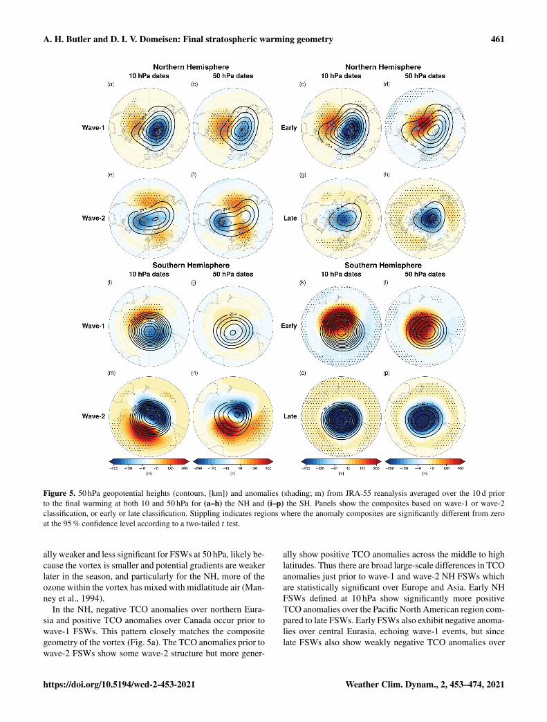
(a and b) show a shift of the polar vortex towards Eura-sia, with corresponding anomalously positive stratosphericheight anomalies over North America. Wave-2 FSWs (e andf) instead show an elongated vortex centered over the poleand extending across Canada to eastern Asia, correspond-ing to anomalously positive stratospheric height anomaliesover the North Pacific and Europe. These features do notshow substantial differences between the 10 and 50 hPa FSWdates. Comparing early (c and d) and late (g and h) events inthe NH indicates that on average early events manifest sim-ilarly to wave-1 events, with a shift of the vortex towardsEurasia. The early events for 10 hPa dates have more signif-icant negative anomalies over Eurasia compared to the earlyevents for 50 hPa dates. Late events on average show a moreannular response representing (by definition) a stronger vor-tex compared to average for those dates, though overall thevortex is smaller and weaker compared to early events.
In the SH (Fig. 5i–p), wave-1 cases (i and j) on averageshow a displacement of the vortex towards the Weddell Sea,with anomalously positive height anomalies south of Aus-tralia. This wave-1 pattern is only significant for the 10 hPadates, while wave-1 events for the 50 hPa dates (generallylater in austral spring) do not as consistently displace thevortex in a preferred location. Wave-2 events (m and n) forboth 10 and 50 hPa dates show negative stratospheric heightanomalies over the South Pacific, with anomalously posi-tive height anomalies south of Africa, but overall the wave-2structure seen in individual cases (Fig. 3g and h) is unclearin the composite (though sample size is small). Robust dif-ferences between early (k and l) and late events (o and p)for both 10 and 50 hPa dates are evident in the SH. Thesedifferences show a broadly weaker than average vortex forearly events and stronger than average vortex for late events,as expected by definition. There is little wave structure to theearly and late events in the SH, though early events are moredisplaced off the pole than late events.
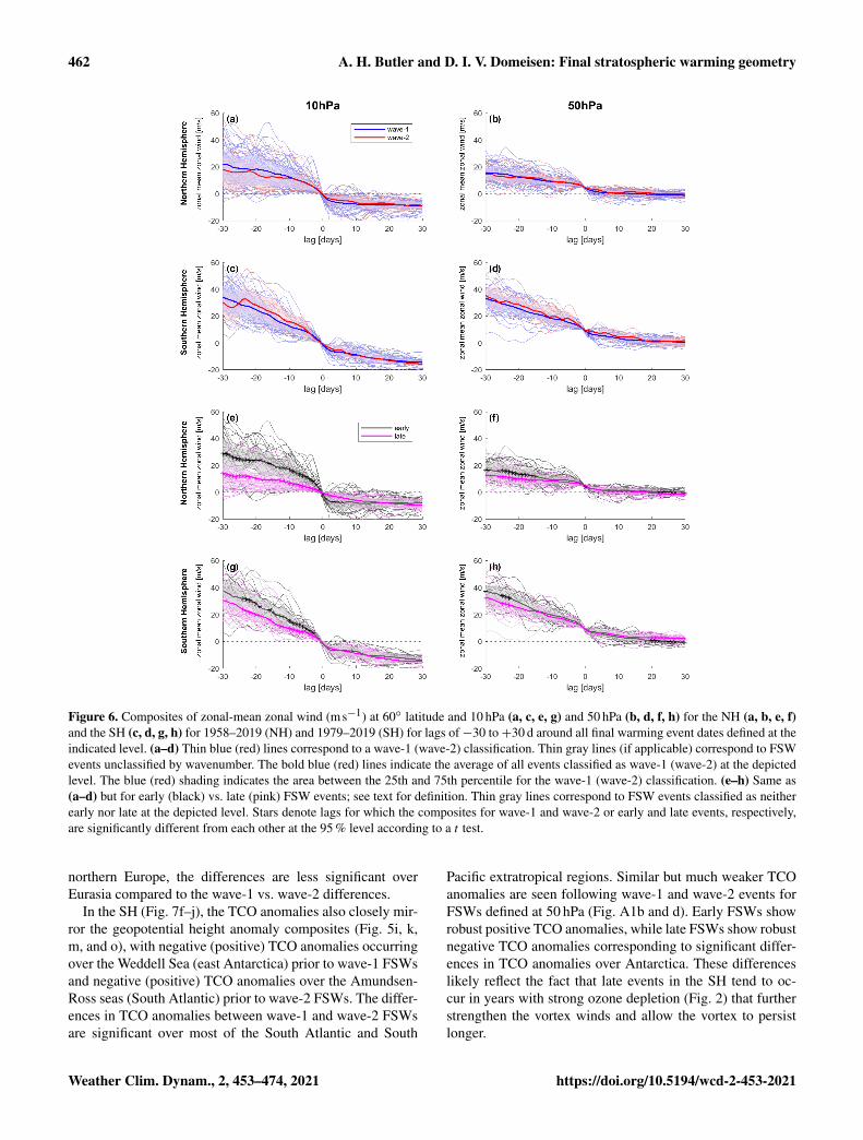
In order to obtain a better comparison of the behavior ofthe zonal-mean zonal winds around the FSW event for thedifferent wave classifications, Fig. 6 shows a composite ofzonal-mean zonal wind for the month before and after theFSW using the date at either 10 hPa (Fig. 6a, c, e, and g) or50 hPa (Fig. 6b, d, f, and h). The wind speeds about a monthbefore the FSW event are weaker in the NH as compared tothe SH (e.g., compare Figs. 6a and b with c and d). In the NHthe winds can already exhibit values close to zero within themonth before the FSW event, while in the SH the winds aresignificantly stronger in the month before the event. The av-erage decrease in wind speed between the average over lagsof −30 to −11 d before the FSW event and days 11 to 30after the event is 25.2 ms−1 (36.7 ms−1) for the NH (SH)at 10 hPa. Further down at 50 hPa, these values are smaller,i.e., 12.8 ms−1 (24.8 ms−1) for the NH (SH). No signifi-cant differences are found in wind speed between wave-1and wave-2 classifications. This suggests that, though the dif-ferent wave geometries are clearly associated with asymme-
tries in the geopotential heights (Fig. 5), the wave geometryhas little influence on the strength of the zonal-mean strato-spheric wind changes.
We then compare this behavior to early vs. late FSWevents. Early FSW events are associated with a stronger de-celeration of the winds as compared to late FSW events at alllevels and in both hemispheres due to the seasonally strongerwinds earlier in the season (Fig. 6e–h). In the NH, the windsare significantly weaker before early FSW events at 50 hPaas compared to 10 hPa, while for late events, the decelerationis weaker at both levels. The decrease in wind speed betweenthe average over lags of −30 to −11 d before the FSW eventand days 11 to 30 after the event is 31.4 ms−1 (13.3 ms−1) at10 (50) hPa for early events. For late events, the correspond-ing values are 18.8 ms−1 (10.8 ms−1) at 10 (50) hPa. In theSH the winds exhibit similar strengths before the FSW eventat both 10 and 50 hPa, although the deceleration at the timeof the FSW event is stronger at 10 hPa compared to 50 hPa.The decrease in wind speed between the average over lagsof −30 to −11 d before the FSW event and days 11 to 30after the event is 39.3 ms−1 (28.3 ms−1) at 10 (50) hPa forearly events. For late events, the corresponding values are33.4 ms−1 (22.8 ms−1) at 10 (50) hPa. The wind speeds at10 hPa between early and late events are significantly dif-ferent from each other for most lags before the FSW event,while at 50 hPa the winds speeds are significantly differentfor early vs. late events only at lags around −20 d or longer.After the FSW event, significant differences can only be de-tected between early and late events for the first few days at10 hPa in the NH.
4 Implications for ozone distribution during springonset
To investigate the influence of final warming wave geometryon total column ozone, we use the Bodeker Scientific filledtotal column ozone (TCO) database (Version 3.4) (Bodekeret al., 2020). This dataset combines measurements from mul-tiple satellite-based instruments and fills missing data with amachine-learning-based method to create a temporally andspatially gap-free database of total column ozone from 31October 1978 to 31 December 2016. We also comparedthese results to the same analysis using ERA-interim ozoneat the 500 K isentrope (lower stratosphere), and the resultswere very similar (not shown). TCO anomalies are calculatedbased on the 1979–2016 daily climatology.
Figure 7a–e show the NH TCO anomalies (from 1979–2016, the period of the ozone dataset) 10 d prior to the finalwarming for the 10 hPa FSW dates and for different classi-fications. A corresponding figure for the 50 hPa FSW datesis shown in the Appendix (Fig. A1), but we found in bothhemispheres that the differences in TCO anomalies tied towave geometry were more apparent for 10 hPa FSW dates.While spatial patterns are similar, TCO anomalies are gener-
A. H. Butler and D. I. V. Domeisen: Final stratospheric warming geometry 461
Figure 5. 50 hPa geopotential heights (contours, [km]) and anomalies (shading; m) from JRA-55 reanalysis averaged over the 10 d priorto the final warming at both 10 and 50 hPa for (a–h) the NH and (i–p) the SH. Panels show the composites based on wave-1 or wave-2classification, or early or late classification. Stippling indicates regions where the anomaly composites are significantly different from zeroat the 95 % confidence level according to a two-tailed t test.
ally weaker and less significant for FSWs at 50 hPa, likely be-cause the vortex is smaller and potential gradients are weakerlater in the season, and particularly for the NH, more of theozone within the vortex has mixed with midlatitude air (Man-ney et al., 1994).
In the NH, negative TCO anomalies over northern Eura-sia and positive TCO anomalies over Canada occur prior towave-1 FSWs. This pattern closely matches the compositegeometry of the vortex (Fig. 5a). The TCO anomalies prior towave-2 FSWs show some wave-2 structure but more gener-
ally show positive TCO anomalies across the middle to highlatitudes. Thus there are broad large-scale differences in TCOanomalies just prior to wave-1 and wave-2 NH FSWs whichare statistically significant over Europe and Asia. Early NHFSWs defined at 10 hPa show significantly more positiveTCO anomalies over the Pacific North American region com-pared to late FSWs. Early FSWs also exhibit negative anoma-lies over central Eurasia, echoing wave-1 events, but sincelate FSWs also show weakly negative TCO anomalies over
462 A. H. Butler and D. I. V. Domeisen: Final stratospheric warming geometry
Figure 6. Composites of zonal-mean zonal wind (ms−1) at 60◦ latitude and 10 hPa (a, c, e, g) and 50 hPa (b, d, f, h) for the NH (a, b, e, f)and the SH (c, d, g, h) for 1958–2019 (NH) and 1979–2019 (SH) for lags of−30 to+30 d around all final warming event dates defined at theindicated level. (a–d) Thin blue (red) lines correspond to a wave-1 (wave-2) classification. Thin gray lines (if applicable) correspond to FSWevents unclassified by wavenumber. The bold blue (red) lines indicate the average of all events classified as wave-1 (wave-2) at the depictedlevel. The blue (red) shading indicates the area between the 25th and 75th percentile for the wave-1 (wave-2) classification. (e–h) Same as(a–d) but for early (black) vs. late (pink) FSW events; see text for definition. Thin gray lines correspond to FSW events classified as neitherearly nor late at the depicted level. Stars denote lags for which the composites for wave-1 and wave-2 or early and late events, respectively,are significantly different from each other at the 95 % level according to a t test.
northern Europe, the differences are less significant overEurasia compared to the wave-1 vs. wave-2 differences.
In the SH (Fig. 7f–j), the TCO anomalies also closely mir-ror the geopotential height anomaly composites (Fig. 5i, k,m, and o), with negative (positive) TCO anomalies occurringover the Weddell Sea (east Antarctica) prior to wave-1 FSWsand negative (positive) TCO anomalies over the Amundsen-Ross seas (South Atlantic) prior to wave-2 FSWs. The differ-ences in TCO anomalies between wave-1 and wave-2 FSWsare significant over most of the South Atlantic and South
Pacific extratropical regions. Similar but much weaker TCOanomalies are seen following wave-1 and wave-2 events forFSWs defined at 50 hPa (Fig. A1b and d). Early FSWs showrobust positive TCO anomalies, while late FSWs show robustnegative TCO anomalies corresponding to significant differ-ences in TCO anomalies over Antarctica. These differenceslikely reflect the fact that late events in the SH tend to oc-cur in years with strong ozone depletion (Fig. 2) that furtherstrengthen the vortex winds and allow the vortex to persistlonger.
A. H. Butler and D. I. V. Domeisen: Final stratospheric warming geometry 463
Figure 7. Composite total column ozone anomaly (Dobson units) averaged over the 10 d prior to FSWs at 10 hPa for (a–e) the NH and (f–j)the SH. Panels show the composites based on (a, f) all events from 1979–2016 (the period of the TCO dataset), (b, g) wave-1 or (d, i) wave-2classification, or (c, h) early or (e, j) late classification. Stippling in (a, f) indicates regions where the anomaly composites are significantlydifferent from zero at the 95 % confidence level according to a two-tailed t test; stippling in other panels shows where composites aresignificantly different from each other (e.g., wave-1 vs. wave-2, early vs. late) using a t test for two samples of unequal variance.
We have shown that both the wave geometry and timing ofthe event can play a role in the evolution of springtime TCOanomalies, which may have implications for ecosystems andhuman health due to increased ultraviolet (UV) radiation ex-posure (Barnes et al., 2019) or stratosphere-to-troposphereozone transport (Albers et al., 2018). For example, prior towave-1 and early NH FSWs there are widespread negativeTCO anomalies over Eurasia and positive TCO anomaliesover North America that are shifted off the pole towards morepopulated areas, compared to wave-2 and late NH FSWs.
5 Surface impacts
There are observed differences in the NH surface impactsfollowing displacement and split-type SSW events (Mitchellet al., 2013), though the robustness of these impacts is de-bated (Maycock and Hitchcock, 2015; Hall et al., 2021;White et al., 2021). To see if such differences exist following
different geometries or timings of final warmings, we nextinvestigate potential differences in the surface impact for dif-ferent types of FSW events. Figure 8 shows the composite re-sponse for wave-1 and wave-2 (and early and late) FSWs forlinearly detrended 500 hPa geopotential height anomalies fordays 7–30 after the 50 hPa FSW event dates. A comparablefigure is shown in the Appendix for 10 hPa dates (Fig. A2).The composites based on the 50 hPa dates are highlightedhere because (1) changes of the vortex in the lower strato-sphere have been linked more closely with changes in tro-pospheric circulation (Maycock and Hitchcock, 2015), and(2) the surface responses are more similar to known patternsassociated with stratosphere–troposphere coupling followingFSWs. The detrending was applied to account for possibletrends in the storm tracks but does not qualitatively changethe results.
The average over all NH FSW events (Fig. 8a) showsa negative NAO-like structure with a high geopotential
464 A. H. Butler and D. I. V. Domeisen: Final stratospheric warming geometry
Figure 8. Composite of the linearly detrended 500 hPa geopotential height anomalies (m) from JRA-55 data for (a, f) all FSW events basedon the 50 hPa dates and classified as (b, g) wave-1, (d, i) wave-2, (c, h) early, or (e, j) late averaged over the 7–30 d after the central FSW date(i.e., lags of 7–30 d) for (a–e) the NH and (f–j) the SH extratropics. Stippling in (a, f) indicates regions where the anomaly composites aresignificantly different from zero at the 95 % confidence level according to a t test, while stippling in other panels shows where compositesare significantly different from each other (e.g., wave-1 vs. wave-2, early vs. late) according to a 1000-sample bootstrap analysis (withreplacement).
anomaly over Greenland and a low geopotential anomalyover Europe and the adjacent North Atlantic region. A posi-tive geopotential height anomaly is observed in the North Pa-cific. When dividing the response between wave-1 and wave-2 (Fig. 8b and d), the negative NAO response persists for bothtypes of events, but the response over North America is op-posite between wave-1 and wave-2 events, with a positive(negative) anomaly over Canada for wave-1 (wave-2) eventsand the opposite response over the southern United States.Wave-2 events also show stronger positive anomalies overthe North Pacific that are significantly different from wave-1events. Early and late FSWs also show opposing but less sig-nificant differences across North America (Fig. 8c and e), butthere are more significant differences in the circulation re-sponse over Eurasia compared to wave-1 vs. wave-2 events.
In the SH, anomalously high geopotential heights arefound across Antarctica surrounded by anomalously lowgeopotential heights over the Southern Ocean in the aver-
age for all events (Fig. 8f), which resembles the negativephase of the Southern Annular Mode (SAM). The same pat-tern is apparent following both wave-1 and wave-2 events(Fig. 8g and i), though the wave-2 composite is noisy dueto few samples. The surface impacts following FSWs areclearly dominated by the timing, not the wave geometry, ofthe FSW (Fig. 8h and j). Early FSWs show a significantlymore negative SAM pattern compared to late FSWs whichshow a positive SAM pattern. Importantly, averaging overall events yields insignificant circulation anomalies (panel f),but this apparent lack of response arises from the cancella-tion of significant differences between early and late events.Overall, greater ozone loss in early austral spring leads to acolder vortex that persists longer (Fig. 2) and keeps ozoneanomalously low until the FSW (Fig. 7j), resulting in a pos-itive SAM and poleward-shifted jet stream into austral sum-mer. Our results support findings that ozone hole recoverysince 2000 has reversed circulation trends due to ozone de-
A. H. Butler and D. I. V. Domeisen: Final stratospheric warming geometry 465
pletion (Banerjee, Antara et al., 2020) towards earlier FSWsand a more negative SAM.
Since the surface signal over the North Atlantic tends toshow a structure reminiscent of the negative phase of theNAO (Fig. 8a), we also composite the NAO index (obtainedfrom the Climate Prediction Center) for the period 1958–2019 using the 50 hPa FSW dates (Fig. 9a). The NAO experi-ences a decrease from significantly positive values before theFSW event to values close to zero or negative starting withina week after the event. Both wave-1 and wave-2 FSW eventsexperience a tendency towards a negative NAO after the cen-tral day of the event, with on average consistently positiveNAO values in the 40 d before the event. Values significantlydifferent from zero are observed primarily for wave-1 eventsfor lags between 5 and 20 d before the FSW event. Wave-2 events show larger variability, especially after the FSWevent, likely due to the smaller sample size as compared towave-1 events. A similar picture emerges when compositingthe NAO for early vs. late events (Fig. 9b). Both early andlate FSW events exhibit a drop in the NAO from positive tonegative values roughly a week after the FSW event. Lateevents show more variability than early events.
6 Conclusions
Both sudden stratospheric warming events in the middle ofwinter and final stratospheric warming events that mark theend of winter in the stratosphere are characterized by a sim-ilar evolution and are often classified by the same metrics,i.e., when the zonal-mean zonal winds of the polar vortexfall below some threshold. However, in order to characterizetheir evolution further, different measures are used. The mostdominant classification for midwinter sudden stratosphericwarmings is by their wave geometry into split and displace-ment events. FSWs, on the other hand, have so far not beenclassified by geometry but only by their timing or verticalevolution. This difference in the classification between mid-winter and end-of-winter polar vortex breakdowns is likelydue to the notion that a wave geometry cannot always beidentified for FSW events, especially for events that occurlater in spring and that are more radiatively driven. We showhere that final warmings can almost exclusively be classifiedwith regard to their geometrical wave structure. This geo-metrical structure is present even for most late events. A de-tailed classification of wave geometry using FSWs detectedat two different pressure levels and for two different reanaly-sis products is provided.
Defining the final warming date at 50 vs. 10 hPa yieldsa much more significant shift in the timing in the SH ascompared to the NH. In particular, using the 50 hPa datesmore clearly captures ozone-related trends in the timing ofthe SH FSWs. On the other hand, the interannual variabil-ity in FSW dates at 10 and 50 hPa is significantly correlatedin both hemispheres. Our analysis suggests that, depending
on the question being explored, there could be valid rea-sons for using either the 10 or 50 hPa dates. For example,for SSWs the 10 hPa level has been found to be optimal fordetecting dynamic changes in the stratospheric circulation,whereas the 50 hPa level shows stronger linkages to surfaceimpacts (Butler and Gerber, 2018). Here, we noted a moresignificant relationship of wave geometry to TCO anomaliesusing the 10 hPa dates but a more expected tropospheric re-sponse when using the 50 hPa dates.
Weaker westerly winds in spring allow for more verticalpropagation of wave-2 and even wave-3 into the stratosphere.Similar to SSWs, more events are characterized as wave-1events as compared to wave-2 events in both hemispheres.Wave-3 plays a more significant role in the NH stratosphereduring the FSW compared to midwinter SSW events, whenwave-3 is generally not able to propagate into the strong vor-tex winds present prior to SSWs. One NH event in 2009 wasclassified as a wave-3 event, and several other events showclear wave-3 structure even in the SH.
To bring together the influence of FSW wave geometryon the polar vortex, TCO anomalies, and tropospheric im-pacts, here we summarize the composite impacts from eachtype of classification. Wave-1 events shift the polar vortexoff the pole preferentially towards Eurasia in the NH and theWeddell Sea in the SH. This is associated with anomalouslyhigh stratospheric heights over Canada in the NH and overeast Antarctica in the SH. The vortex shift is associated withanomalously low total column ozone in the region where theozone-poor vortex air shifts towards and anomalously hightotal column ozone in the region it moves away from. Wave-1 events are followed in the NH by a negative NAO-like pat-tern in the North Atlantic, positive 500 hPa height anomaliesover Canada, and negative 500 hPa height anomalies over theUnited States.
Wave-2 events in the NH generally consist of an elongatedor split vortex preferentially over Canada and eastern Asia,with anomalously high stratospheric heights over the NorthPacific and European sectors. In the SH, the vortex evolu-tion is less consistent for wave-2, but on average there areanomalously high stratospheric heights south of Africa andnegative heights over the South Pacific. Wave-2 events areassociated with broadly positive total column ozone anoma-lies in both hemispheres. For surface impacts, NH wave-2events are followed by anomalously positive 500 hPa heightanomalies over the North Pacific and United States, oppo-sitely signed to wave-1 events, though the negative NAO pat-tern is consistent.
From our results, it is evident that the FSW wave ge-ometry could be relevant for understanding and predictingthe evolution of total column ozone anomalies in spring. Inparticular, wave-1 events tend to be associated with morewidespread negative TCO anomalies prior to the FSW thanwave-2 events in both hemispheres. This may be because,while wave-2 events tend to be associated with elongationand possible splitting over the pole, wave-1 events displace
466 A. H. Butler and D. I. V. Domeisen: Final stratospheric warming geometry
Figure 9. Composite of the NAO index (using a 3 d running mean) for lags of −40 to +40 d around the final warming dates at 50 hPa for1958–2019. (a) The blue (red) lines indicate the average values for the wave-1 (wave-2) classifications, respectively. The dashed gray line isthe average over all FSW events from 1958–2019, including unclassified events. Bold parts of the lines indicate values significantly differentfrom zero at the 95 % level according to a t test. The blue (red) shading indicates the 25th and 75th percentiles for the wave-1 (wave-2)classification. (b) Same as (a) but for early (black) vs. late (purple) FSW events.
the vortex equatorward into more sunlit regions. Still, thetiming of the FSW is also very important; in the SH, differ-ences in polar cap TCO anomalies for early and late eventsare likely associated with chemistry–climate feedbacks thatplay a central role in stratosphere–troposphere coupling inaustral spring. Consideration of both the timing and geom-etry of the FSW in both hemispheres may be important forhow much stratospheric ozone is available to be transportedvia deep stratospheric intrusions to the surface in spring (Al-bers et al., 2018; Breeden et al., 2020).
While there are some indications of the modulation of tro-pospheric impacts by FSW wave geometry, in general FSWsof either wave classification are followed by a shift towardsthe negative phase of the NAO in the NH and the SAM in theSH. We did not attempt to identify causes for the differentsurface response over, for example, North America, whichcould be linked to tropospheric variability leading up to theFSWs, the more direct influence of the stratospheric wavegeometry on the underlying tropospheric circulation, or toother large-scale climate patterns like El Niño–Southern Os-
cillation (Domeisen et al., 2019) or decadal variability. Thesesignals may also arise due to sampling given the small num-ber of events available in the historical record; further testingwith long model simulations may reveal non-significant dif-ferences (e.g., Maycock and Hitchcock, 2015). Troposphericimpacts are strongly tied to the timing of the FSW in the SH,where the tropospheric height pattern is nearly the mirror op-posite for early and late FSWs. These differences are likelyrelated to the trends associated with ozone depletion and re-covery that have been linked both to trends in the timing ofSH FSWs and to changes in atmospheric circulation.
The ability to classify final stratospheric warming eventsby wave geometry points out similarities with midwinter sud-den stratospheric warming events, while the greater impor-tance of wave-3 for FSWs highlights the differences. Wehave shown that the structure of the stratospheric polar vor-tex as it weakens in spring can influence total column ozoneand tropospheric impacts, suggesting that the wave geome-try of FSWs may be important for improving predictive skillfollowing these events. Whether the wave geometry charac-
A. H. Butler and D. I. V. Domeisen: Final stratospheric warming geometry 467
teristics of FSWs are well simulated in climate and forecastmodels, and if they are modulated by external forcings likeincreasing greenhouse gases, should be investigated.
468 A. H. Butler and D. I. V. Domeisen: Final stratospheric warming geometry
Appendix A
Table A1. Details of JRA-55 classification for 1979–2019 using NH final warming dates based on 60◦ N and 10 hPa. The two metricsdetermine the wavenumber (WN) with maximum mean amplitude and highest percent of days of maximum amplitude for the 10 d before theFSW, as described in Sect. 2. U= unclassified (methods did not agree according to the criterion outlined in Sect. 2).
A. H. Butler and D. I. V. Domeisen: Final stratospheric warming geometry 469
Figure A1. Composite total column ozone anomaly (Dobson units) averaged over the 10 d prior to FSWs at 50 hPa for (a–e) the NH and (f–j)the SH. Panels show the composites based on (a, f) all events from 1979–2016 (the period of the TCO dataset), (b, g) wave-1 or (d, i) wave-2classification, or (c, h) early or (e, j) late classification. Stippling in (a, f) indicates regions where the anomaly composites are significantlydifferent from zero at the 95 % confidence level on a two-tailed t test; stippling in other panels shows where composites are significantlydifferent from each other (e.g., wave-1 vs. wave-2, early vs. late) using a t test for two samples of unequal variance.
470 A. H. Butler and D. I. V. Domeisen: Final stratospheric warming geometry
Figure A2. Composite of the linearly detrended 500 hPa geopotential height anomalies (m) from JRA-55 data for (a, f) all FSW events basedon the 10 hPa dates and classified as (b, g) wave-1, (d, i) wave-2, (c, h) early, or (e, j) late averaged over the 7–30 d after the central FSW date(i.e., lags of 7–30 d) for (a–e) the NH and (f–j) the SH extratropics. Stippling in (a, f) indicates regions where the anomaly composites aresignificantly different from zero at the 95 % confidence level according to a t test, while stippling in other panels shows where compositesare significantly different from each other (e.g., wave-1 vs. wave-2, early vs. late) according to a 1000-sample bootstrap analysis (withreplacement).
A. H. Butler and D. I. V. Domeisen: Final stratospheric warming geometry 471
Data availability. The ERA-interim Reanalysis datawere obtained from the ECMWF data portal at https://apps.ecmwf.int/datasets/data/interim-full-daily/ (Berrisfordet al., 2011). The JRA-55 data were obtained from the NCARResearch Data Archive at https://doi.org/10.5065/D6HH6H41(Japan Meteorological Agency/Japan, 2013). The NAO indexwas obtained from the Climate Prediction Center at https://www.cpc.ncep.noaa.gov/products/precip/CWlink/pna/nao.shtml(National Oceanic and Atmospheric Administration, ClimatePrediction Center, 2021). The total column ozone database wasobtained from https://doi.org/10.5281/zenodo.3908787 (Bodekeret al., 2020). We would like to thank Bodeker Scientific, fundedby the New Zealand Deep South National Science Challenge, forproviding the combined NIWA-BS total column ozone database.
Author contributions. The authors together initiated and designedthe study. Both authors contributed to figures, and both contributedto the writing.
Competing interests. The authors declare that they do not have anycompeting interests.
Acknowledgements. The authors thank Darryn Waugh, Nick Byrne,and an anonymous reviewer, as well as the co-editor Yang Zhang,for their helpful comments during the discussion phase.
Financial support. Amy H. Butler has been supported by the Na-tional Science Foundation (grant no. 1756958) and Daniela I. V.Domeisen by the Swiss National Science Foundation (grant no.PP00P2_170523).
Review statement. This paper was edited by Yang Zhang and re-viewed by Darryn Waugh and one anonymous referee.
References
Afargan-Gerstman, H. and Domeisen, D. I. V.: Pacific Modula-tion of the North Atlantic Storm Track Response to SuddenStratospheric Warming Events, Geophys. Res. Lett., 47, 18–10,https://doi.org/10.1029/2019GL085007, 2020.
Albers, J. R., Perlwitz, J., Butler, A. H., Birner, T., Kiladis, G. N.,Lawrence, Z. D., Manney, G. L., Langford, A. O., and Dias, J.:Mechanisms Governing Interannual Variability of Stratosphere-to-Troposphere Ozone Transport, J. Geophys. Res.-Atmos., 123,234–260, 2018.
Ayarzagüena, B. and Serrano, E.: Monthly Characterization of theTropospheric Circulation over the Euro-Atlantic Area in Relationwith the Timing of Stratospheric Final Warmings, J. Climate, 22,6313–6324, 2009.
Baldwin, M. P., Ayarzaguena, B., Birner, T., Butchart, N., Butler,A. H., Charlton-Perez, A. J., Domeisen, D. I. V., Garfinkel, C. I.,Garny, H., Gerber, E. P., Hegglin, M. I., Langematz, U., and Pe-
datella, N. M.: Sudden Stratospheric Warmings, Rev. Geophys.,59, 27.1–37, 2021.
Bancalá, S., Krüger, K., and Giorgetta, M.: The preconditioningof major sudden stratospheric warmings, J. Geophys. Res., 117,D04101, https://doi.org/10.1029/2011JD016769, 2012.
Banerjee, A., Fyfe, J. C, Polvani, L. M., Waugh, D., and Chang, K-L.: A pause in Southern Hemisphere circulation trends due to theMontreal Protocol., Nat. Geosci., 579, 544–548, 2020.
Barnes, P. W., Williamson, C. E., Lucas, R. M., Robinson, S. A.,Madronich, S., Paul, N. D., Bornman, J. F., Bais, A. F.,Sulzberger, B., Wilson, S. R., Andrady, A. L., McKenzie, R. L.,Neale, P. J., Austin, A. T., Bernhard, G. H., Solomon, K. R.,Neale, R. E., Young, P. J., Norval, M., Rhodes, L. E., Hylan-der, S., Rose, K. C., Longstreth, J., Aucamp, P. J., Ballaré, C. L.,Cory, R. M., Flint, S. D., de Gruijl, F. R., Häder, D.-P., Heikkilä,A. M., Jansen, M. A. K., Pandey, K. K., Robson, T. M., Sinclair,C. A., Wängberg, S.-Å., Worrest, R. C., Yazar, S., Young, A. R.,and Zepp, R. G.: Ozone depletion, ultraviolet radiation, climatechange and prospects for a sustainable future, Nature Sustain-ability, 2, 569–579, 2019.
Barriopedro, D. and Calvo, N.: On the Relationship between ENSO,Stratospheric Sudden Warmings, and Blocking, J. Climate, 27,4704–4720, 2014.
Berrisford, P., Dee, D. P., Poli, P., Brugge, R., Fielding, M., Fuentes,M., Kållberg, P. W., Kobayashi, S., Uppala, S., and Simmons,A.: The ERA-Interim archive Version 2.0, ERA Report Series,https://www.ecmwf.int/node/8174 (last access: 21 May 2021).
Black, R., McDaniel, B., and Robinson, W. A.: Stratosphere-troposphere coupling during spring onset, J. Climate, 19, 4891–4901, 2006.
Black, R. X. and McDaniel, B.: Interannual Variability in the South-ern Hemisphere Circulation Organized by Stratospheric FinalWarming Events, J. Atmos. Sci., 64, 2968–2974, 2007a.
Black, R. X. and McDaniel, B. A.: The dynamics of northern hemi-sphere stratospheric final warming events, J. Atmos. Sci., 64,2932–2946, 2007b.
Bodeker, G. E., Kremser, S., and Tradowsky, J. S.: BS FilledTotal Column Ozone Database (Version 3.4) [data set],https://doi.org/10.5281/zenodo.3908787, 2020.
Breeden, M. L., Butler, A. H., Albers, J. R., Sprenger, M., and Lang-ford, A. O.: The spring transition of the North Pacific jet and itsrelation to deep stratosphere-to-troposphere mass transport overwestern North America, Atmos. Chem. Phys., 21, 2781–2794,https://doi.org/10.5194/acp-21-2781-2021, 2021.
Butler, A. H. and Gerber, E. P.: Optimizing the definition of a sud-den stratospheric warming, J. Climate, 31, 2337–2344, 2018.
Butler, A. H., Seidel, D. J., Hardiman, S. C., Butchart, N., Birner,T., and Match, A.: Defining sudden stratospheric warmings, B.Am. Meteorol. Soc., 96, 1913–1928, 2015.
Butler, A. H., Sjoberg, J. P., Seidel, D. J., and Rosenlof, K. H.:A sudden stratospheric warming compendium, Earth Syst. Sci.Data, 9, 63–76, https://doi.org/10.5194/essd-9-63-2017, 2017.
Butler, A. H., Charlton-Perez, A., Domeisen, D. I. V., Simpson,I., and Sjoberg, J.: Predictability of Northern Hemisphere finalstratospheric warmings and their surface impacts, Geophys. Res.Lett., 46, https://doi.org/10.1029/2019GL083346, 2019.
Byrne, N. J. and Shepherd, T. G.: Seasonal Persistence of Circu-lation Anomalies in the Southern Hemisphere Stratosphere and
472 A. H. Butler and D. I. V. Domeisen: Final stratospheric warming geometry
Its Implications for the Troposphere, J. Climate, 31, 3467–3483,2018.
Byrne, N. J., Shepherd, T. G., Woollings, T., and Plumb, R. A.:Nonstationarity in Southern Hemisphere Climate Variability As-sociated with the Seasonal Breakdown of the Stratospheric PolarVortex, J. Climate, 30, 7125–7139, 2017.
Byrne, N. J., Shepherd, T. G., and Polichtchouk, I.: Subseasonal-to-Seasonal Predictability of the Southern Hemisphere Eddy-Driven Jet During Austral Spring and Early Summer, J. Geophys.Res.-Atmos., 124, 6841–6855, 2019.
Calvo, N., Polvani, L. M., and Solomon, S.: On the surface impactof Arctic stratospheric ozone extremes, Environ. Res. Lett., 10,https://doi.org/10.1088/1748-9326/10/9/094003, 2015.
Charlton, A. and Polvani, L. M.: A new look at stratospheric sud-den warmings. Part I: Climatology and modeling benchmarks, J.Climate, 20, 449–469, 2007.
Charlton, A., O’Neill, A., Lahoz, W., and Berrisford, P.: The split-ting of the stratospheric polar vortex in the Southern Hemisphere,September 2002: Dynamical evolution, J. Atmos. Sci., 62, 590–602, 2005.
Charlton-Perez, A. J., Ferranti, L., and Lee, R. W.: The influence ofthe stratospheric state on North Atlantic weather regimes, Q. J.Roy. Meteor. Soc., 144, 1140–1151, 2018.
Charney, J. and Drazin, P.: Propagation of planetary-scale distur-bances from the lower into the upper atmosphere, J. Geophys.Res., 66, 83–109, 1961.
Chipperfield, M. P. and Jones, R. L.: Relative influences of atmo-spheric chemistry and transport on Arctic ozone trends, Nature,400, 551–554, 1999.
Coy, L., Nash, E. R., and Newman, P. A.: Meteorology of the polarvortex: Spring 1997, Geophys. Res. Lett., 24, 2693–2696, 1997.
Dee, D. P., Uppala, S. M., Simmons, A. J., Berrisford, P., Poli,P., Kobayashi, S., Andrae, U., Balmaseda, M. A., Balsamo, G.,Bauer, P., Bechtold, P., Beljaars, A. C. M., van de Berg, L., Bid-lot, J., Bormann, N., Delsol, C., Dragani, R., Fuentes, M., Geer,A. J., Haimberger, L., Healy, S. B., Hersbach, H., Holm, E. V.,Isaksen, L., Kallberg, P., Köhler, M., Matricardi, M., McNally,A. P., Monge-Sanz, B. M., Morcrette, J.-J., Park, B.-K., Peubey,C., de Rosnay, P., Tavolato, C., Thepaut, J.-N., and Vitart, F.:The ERAInterim reanalysis: Configuration and performance ofthe data assimilation system, Q. J. Roy. Meteor. Soc., 137, 553–597, 2011.
Domeisen, D. I. V.: Estimating the Frequency of Sudden Strato-spheric Warming Events from Surface Observations of the NorthAtlantic Oscillation, J. Geophys. Res.-Atmos., 124, 3180–3194,https://doi.org/10.1029/2018JD030077, 2019.
Domeisen, D. I. V. and Butler, A. H.: Stratospheric drivers of ex-treme events at the Earth’s surface, Communications Earth &Environment, 1, 59, https://doi.org/10.1038/s43247-020-00060-z, 2020.
Domeisen, D. I. V., Garfinkel, C. I., and Butler, A. H.: The Telecon-nection of El Niño Southern Oscillation to the Stratosphere, Rev.Geophys., 57, 5–47, https://doi.org/10.1029/2018RG000596,2019.
Domeisen, D. I. V., Butler, A. H., Charlton-Perez, A. J.,Ayarzaguena, B., Baldwin, M. P., Dunn Sigouin, E., Furtado,J. C., Garfinkel, C. I., Hitchcock, P., Karpechko, A. Y., Kim,H., Knight, J., Lang, A. L., Lim, E.-P., Marshall, A., Roff, G.,Schwartz, C., Simpson, I. R., Son, S.-W., and Taguchi, M.: The
Role of the Stratosphere in Subseasonal to Seasonal Prediction:1. Predictability of the Stratosphere, J. Geophys. Res.-Atmos.,125, 1–17, 2020.
Gerber, E. P. and Martineau, P.: Quantifying the variabil-ity of the annular modes: reanalysis uncertainty vs. sam-pling uncertainty, Atmos. Chem. Phys., 18, 17099–17117,https://doi.org/10.5194/acp-18-17099-2018, 2018.
Gerber, E. P., Martineau, P., Ayarzagüena, B., Barriopedro, D.,Bracegirdle, T. J., Butler, A. H., Calvo, N., Hardiman, S. C.,Hitchcock, P., Iza, M., Langematz, U., Lua, H., Marshall, G., Orr,A., Palmeiro, F. M., Son, S.-W., and Taguchi, M.: Extratropicalstratosphere-troposphere coupling, in: Stratosphere-troposphereprocesses and their role in climate (SPARC) reanalysis intercom-parison project (S-RIP), edited by: Fujiwara, M., Manney, G. L.,Gray, L., and Wright, J. S., chap. 6, SPARC, Oberpfaffenhofen,Germany, in press, 2021.
Haigh, J. D. and Roscoe, H. K.: The Final Warming Date of theAntarctic Polar Vortex and Influences on its Interannual Variabil-ity, J. Climate, 22, 5809–5819, 2009.
Hall, R. J., Mitchell, D. M., Seviour, W. J. M., and Wright,C. J.: Tracking the stratosphere-to-surface impact of Sud-den Stratospheric Warmings, J. Geophys. Res.-Atmos., 126,e2020JD033881, 1–47, 2021.
Hardiman, S. C., Butchart, N., Charlton-Perez, A. J., Shaw, T. A.,Akiyoshi, H., Baumgaertner, A., Bekki, S., Braesicke, P., Chip-perfield, M., Dameris, M., Garcia, R. R., Michou, M., Pawson,S., Rozanov, E., and Shibata, K.: Improved predictability of thetroposphere using stratospheric final warmings, J. Geophys. Res.,116, 6313, https://doi.org/10.1029/2011JD015914, 2011.
Harvey, V. L., Pierce, R. B., Fairlie, T. D., and Hitch-man, M. H.: A climatology of stratospheric polar vor-tices and anticyclones, J. Geophys. Res.-Atmos., 107,https://doi.org/10.1029/2001JD001471, 2002.
Hu, J. G., Ren, R. C., and Xu, H. M.: Occurrence of Winter Strato-spheric Sudden Warming Events and the Seasonal Timing ofSpring Stratospheric Final Warming, J. Atmos. Sci., 71, 2319–2334, 2014.
Ialongo, I., Sofieva, V., Kalakoski, N., Tamminen, J., and Kyrölä,E.: Ozone zonal asymmetry and planetary wave characterizationduring Antarctic spring, Atmos. Chem. Phys., 12, 2603–2614,https://doi.org/10.5194/acp-12-2603-2012, 2012.
Ivy, D. J., Solomon, S., Calvo, N., and Thompson, D. W. J.: Ob-served connections of Arctic stratospheric ozone extremes toNorthern Hemisphere surface climate, Environ. Res. Lett., 12,024004, https://doi.org/10.1029/2001JD001471, 2017.
Japan Meteorological Agency/Japan: JRA-55: Japanese 55-yearReanalysis, Daily 3-Hourly and 6-Hourly Data, Research DataArchive at the National Center for Atmospheric Research,Computational and Information Systems Laboratory [data set],https://doi.org/10.5065/D6HH6H41 (last access: 21 May 2021),2013, updated monthly.
Karpechko, A. Y.: Predictability of Sudden Stratospheric Warmingsin the ECMWF Extended-Range Forecast System, Mon. WeatherRev., 146, 1063–1075, 2018.
Karpechko, A. Y., Hitchcock, P., Peters, D. H. W., and Schnei-dereit, A.: Predictability of downward propagation of major sud-den stratospheric warmings, Q. J. Roy. Meteor. Soc., 104, 30937,https://doi.org/10.1002/qj.3017, 2017.
A. H. Butler and D. I. V. Domeisen: Final stratospheric warming geometry 473
Karpechko, A. Y., Perez, A. C., Balmaseda, M., Tyrrell, N.,and Vitart, F.: Predicting Sudden Stratospheric Warm-ing 2018 and its Climate Impacts with a Multi-ModelEnsemble, Geophys. Res. Lett., 45, 2018GL081091,https://doi.org/10.1029/2018GL081091, 2018.
Kobayashi, S., Ota, Y., Harada, Y., Ebita, A., Moriya, M., Onoda,H., Onogi, K., Kamahori, H., Kobayashi, C., Endo, H., Miyaoka,K., and Takahashi, K.: The JRA-55 Reanalysis: General Specifi-cations and Basic Characteristics, J. Meteorol. Soc. Jpn. Ser. II,93, 5–48, https://doi.org/10.2151/jmsj.2015-001, 2015.
Kodera, K., Mukougawa, H., Maury, P., Ueda, M., and Claud, C.:Absorbing and reflecting sudden stratospheric warming eventsand their relationship with tropospheric circulation, J. Geophys.Res.-Atmos., 121, 80–94, 2016.
Kravchenko, V. O., Evtushevsky, O. M., Grytsai, A. V., Klekociuk,A. R., Milinevsky, G. P., and Grytsai, Z. I.: Quasi-stationary plan-etary waves in late winter Antarctic stratosphere temperature as apossible indicator of spring total ozone, Atmos. Chem. Phys., 12,2865–2879, https://doi.org/10.5194/acp-12-2865-2012, 2012.
Lawrence, Z. D., Perlwitz, J., Butler, A. H., Manney, G. L., New-man, P. A., Lee, S. H., and Nash, E. R.: The RemarkablyStrong Arctic Stratospheric Polar Vortex of Winter 2020: Linksto Record-Breaking Arctic Oscillation and Ozone Loss, J. Geo-phys. Res.-Atmos., 125, 1–29, 2020.
Lim, E. P., Hendon, H. H., and Thompson, D. W. J.: SeasonalEvolution of Stratosphere-Troposphere Coupling in the South-ern Hemisphere and Implications for the Predictability of SurfaceClimate, J. Geophys. Res.-Atmos., 123, 12002–12016, 2018.
Manney, G. L. and Lawrence, Z. D.: The major stratospheric finalwarming in 2016: dispersal of vortex air and termination of Arc-tic chemical ozone loss, Atmos. Chem. Phys., 16, 15371–15396,https://doi.org/10.5194/acp-16-15371-2016, 2016.
Manney, G. L., Farrara, J. D., and Mechoso, C. R.: The behaviorof wave 2 in the Southern Hemisphere stratosphere during latewinter and early spring, J. Atmos. Sci., 48, 976–998, 1991.
Manney, G. L., Zurek, R. W., O’Neill, A., and Swinbank, R.: On themotion of air through the stratospheric polar vortex, J. Atmos.Sci., 51, 2973–2994, 1994.
Matsuno, T.: Vertical Propagation of Stationary Planetary Waves inthe Winter Northern Hemisphere, J. Atmos. Sci., 27, 871–883,1970.
Maycock, A. C. and Hitchcock, P.: Do split and displacement sud-den stratospheric warmings have different annular mode signa-tures?, Geophys. Res. Lett., 42, 10943–10951, 2015.
Mechoso, C. R., O’Neill, A., Pope, V. D., and Farrara, J. D.: A Studyof the Stratospheric Final Warming of 1982 in the Southern-Hemisphere, Q. J. Roy. Meteor. Soc., 114, 1365–1384, 1988.
Mitchell, D. M., Charlton-Perez, A. J., and Gray, L. J.: Characteriz-ing the Variability and Extremes of the Stratospheric Polar Vor-tices Using 2D Moment Analysis, J. Atmos. Sci., 68, 1194–1213,2011.
Mitchell, D. M., Gray, L. J., Anstey, J., Baldwin, M. P., andCharlton-Perez, A. J.: The Influence of Stratospheric Vortex Dis-placements and Splits on Surface Climate, J. Climate, 26, 2668–2682, 2013.
National Oceanic and Atmospheric Administration, Climate Pre-diction Center: The North Atlantic Oscillation index [data set],https://www.cpc.ncep.noaa.gov/products/precip/CWlink/pna/nao.shtml, last access: 21 May 2021.
Newman, P. A.: The final warming and polar vortex disappearanceduring the Southern Hemisphere spring, Geophys. Res. Lett., 13,1228–1231, 1986.
Newman, P. A., Nash, E., and Rosenfield, J.: What controls the tem-perature of the Arctic stratosphere during the spring?, J. Geo-phys. Res., 106, 19999–20010, 2001.
Plumb, R. A.: On the seasonal cycle of stratospheric planetarywaves, Pure Appl. Geophys., 130, 233–242, 1989.
Plumb, R. A.: Planetary waves and the extratropical winter strato-sphere, in: The Stratosphere, Dynamics, Transport and Chem-istry, 190, 23–41, Geophysical Monograph, American Geophys-ical Union, Washington, D. C., 2010.
Randel, W.: The seasonal evolution of planetary waves in the South-ern Hemisphere stratosphere and troposphere, Q. J. Roy. Meteor.Soc., 114, 1385–1409, 1988.
Reichler, T., Kim, J., Manzini, E., and Kröger, J.: A stratosphericconnection to Atlantic climate variability, Nat. Geosci., 5, 783–787, 2012.
Rood, R. B. and Schoeberl, M. R.: Ozone transport by diabaticand planetary wave circulations on a β plane, J. Geophys. Res.-Atmos., 88, 8491–8504, 1983.
Runde, T., Dameris, M., Garny, H., and Kinnison, D. E.: Classifica-tion of stratospheric extreme events according to their downwardpropagation to the troposphere, Geophys. Res. Lett., 43, 6665–6672, 2016.
Salby, M. L. and Callaghan, P. F.: Influence of planetary wave activ-ity on the stratospheric final warming and spring ozone, J. Geo-phys. Res.-Atmos., 112, 351, 2007.
Savenkova, E. N., Kanukhina, A. Y., Pogoreltsev, A. I., and Mer-zlyakov, E. G.: Variability of the springtime transition date andplanetary waves in the stratosphere, J. Atmos. Sol.-Terr. Phy.,90–91, 1–8, 2012.
Scott, R. and Haynes, P.: The seasonal cycle of planetary waves inthe winter stratosphere, J. Atmos. Sci., 59, 803–822, 2002.
Seviour, W. J. M., Mitchell, D. M., and Gray, L. J.: A practicalmethod to identify displaced and split stratospheric polar vortexevents, Geophys. Res. Lett., 40, 5268–5273, 2013.
Sheshadri, A., Plumb, R. A., and Domeisen, D. I. V.: Canthe delay in Antarctic polar vortex breakup explain recenttrends in surface westerlies?, J. Atmos. Sci., 71, 566–573,https://doi.org/10.1175/JAS-D-12-0343.1, 2014.
Solomon, S.: Stratospheric ozone depletion: A review of conceptsand history, Rev. Geophys., 37, 275–316, 1999.
Solomon, S., Haskins, J., Ivy, D. J., and Min, F.: Fundamental dif-ferences between Arctic and Antarctic ozone depletion, P. Natl.Acad. Sci. USA, 111, 6220–6225, 2014.
Son, S.-W., Purich, A., Hendon, H. H., Kim, B.-M., and Polvani,L. M.: Improved seasonal forecast using ozone hole variability?,Geophys. Res. Lett., 40, 6231–6235, 2013.
Sun, L., Robinson, W. A., and Chen, G.: The role of planetary wavesin the downward influence of stratospheric final warming events,J. Atmos. Sci., 68, 2826–2843, 2011.
Taguchi, M.: Predictability of Major Stratospheric Sudden Warm-ings of the Vortex Split Type: Case Study of the 2002 SouthernEvent and the 2009 and 1989 Northern Events, J. Atmos. Sci.,71, 2886–2904, 2014.
Taguchi, M.: Connection of predictability of major stratosphericsudden warmings to polar vortex geometry, Atmos. Sci. Lett.,17, 33–38, 2016.
474 A. H. Butler and D. I. V. Domeisen: Final stratospheric warming geometry
Thompson, D. W. J., Solomon, S., Kushner, P., England, M., Grise,K., and Karoly, D.: Signatures of the Antarctic ozone hole inSouthern Hemisphere surface climate change, Nat. Geosci., 4,741–749, 2011.
Vargin, P. N., Kostrykin, S. V., Rakushina, E. V., Volodin, E. M.,and Pogoreltsev, A. I.: Study of the Variability of Spring BreakupDates and Arctic Stratospheric Polar Vortex Parameters fromSimulation and Reanalysis Data, Izvestiya, Atmospheric andOceanic Physics, 56, 458–469, 2020.
Wang, T., Zhang, Q., Hannachi, A., Lin, Y., and Hirooka, T.: On thedynamics of the spring seasonal transition in the two hemispherichigh-latitude stratosphere, Tellus A, 71, 1–18, 2019.
Waugh, D. W.: Elliptical diagnostics of stratospheric polar vortices,Q. J. Roy. Meteor. Soc., 123, 1725–1748, 1997.
Waugh, D. W. and Randel, W.: Climatology of Arctic and Antarc-tic polar vortices using elliptical diagnostics, J. Atmos. Sci., 56,1594–1613, 1999.
Waugh, D. W. and Rong, P. P.: Interannual variability in the decayof lower stratospheric Arctic vortices, J. Meteorol. Soc. Jpn., 80,997–1012, 2002.
Waugh, D. W., Randel, W. J., Pawson, S., Newman, P. A., and Nash,E. R.: Persistence of the lower stratospheric polar vortices, J.Geophys. Res.-Atmos., 104, 27191–27201, 1999.
White, I. P., Garfinkel, C. I., Cohen, J., Jucker, M., and Rao,J.: The impact of split and displacement sudden stratosphericwarmings on the troposphere, J. Geophys. Res.-Atmos., 126,e2020JD033989, https://doi.org/10.1029/2020JD033989, 2021.
Zhang, Y., Li, J., and Zhou, L.: The Relationship between PolarVortex and Ozone Depletion in the Antarctic Stratosphere duringthe Period 1979–2016, Adv. Meteorol., 2017, 1–12, 2017.
Zhou, S., Gelman, M. E., Miller, A. J., and McCormack, J. P.: Aninter-hemisphere comparison of the persistent stratospheric polarvortex, Geophys. Res. Lett., 27, 1123–1126, 2000.