Resource Management

WP-RM-09

The World Gas Model:

A Multi-Period Mixed Complementarity Model

for the Global Natural Gas Market

Ruud Egging, Franziska Holz, Steven A. Gabriel

German Institute for Chair for Energy Economics and Economic Research Public Sector Management

The World Gas Model

A Multi-Period Mixed Complementarity Model

for the Global Natural Gas Market

Ruud Egging^, Franziska Holz#, Steven A. Gabriel*

Abstract

We provide the description and illustrative results of the World Gas Model, a multi-period

complementarity model for the global natural gas market. Market players include

producers, traders, pipeline and storage operators, LNG liquefiers and regasifiers as well as

marketers. The model data set contains more than 80 countries and regions and covers 98%

of world wide natural gas production and consumption. We also include a detailed

representation of cross-border natural gas pipelines and constraints imposed by long-term

contracts in the LNG market. The Base Case results of our numerical simulations show that

the rush for LNG observed in the past years will not be sustained throughout 2030 and that

Europe will continue to rely on pipeline gas for a large share of its imports and

consumption.

^ Corresponding author: regging@umd.edu, 1143 Glenn L. Martin Hall, Dept of Civil &

Environmental Engineering, University of Maryland, College Park, MD 20742-3021 USA. # DIW Berlin, Mohrenstr. 58, 10117 Berlin, Germany.

* University of Maryland College Park, and DIW Berlin.

We would like to thank Christian von Hirschhausen for his continuous support and input to the model development effort. We are grateful to the Energy Information Agency and Sophia Rüster and Anne Neumann of TU Dresden for providing us data. Last but not least, we thank Daniel Huppmann for his committed help with the simulation runs and the model documentation. We acknowledge funding by the TransCoop program of the Alexander von Humboldt Foundation and NSF grant n° DMS 0408943.

Page 1 of 36

Page 2 of 36

1 Introduction

The World Gas Model (WGM) is a multi-period numerical equilibrium model of the

global natural gas market covering the next three decades. It includes more than 80

countries and over 98% of global natural gas production and consumption (in 2005, BP

2008). The WGM allows for endogenous investments in pipelines and storage capacities,

as well as for expansion of regasification and liquefaction capacities and considers

demand growth, production capacity expansions and price and cost increases over time.

Taking into account the game-theoretic aspects of the imperfectly competitive natural gas

market, the model includes market power à la Cournot for some players participating in

natural gas trade (i.e., traders and regasifiers.)

This paper documents the 2008 version of the World Gas Model that was used in

Egging et al. (2009) and Huppmann et al. (2009). This model was based on the work of

Gabriel et al. (2005a, b) which established existence and uniqueness results for a class of

gas market models and then applied their model to the North American market.

Huppmann and Egging (2009) provide a more detailed programmers’ and user

manual. WGM is a deterministic model, assuming perfect information and foresight. A

stochastic extension of the WGM was presented in Egging and Holz (2009).

Compared to earlier equilibrium models of international natural gas markets (e.g.,

Egging et al. 2008, Lise and Hobbs 2008, Holz et al. 2008, Zwart 2009), the World Gas

Model is unique with its combination of:

the level of detail for the market agents,

the level of detail for the transport options (pipeline, LNG),

the breadth of the regional coverage,

the multi-period approach with endogenous capacity expansions,

the inclusion of multiple seasons and seasonal arbitrage by storage operators,

the representation of market power.

The World Gas Model is formulated as a mixed complementarity problem (MCP).

The concept of MCP is briefly introduced in the following paragraph.

Page 3 of 36

1.1 Mixed Complementarity Problems

Complementarity modeling provides a very general mathematical framework that can be

applied in many different fields. Cottle et al. (1992) and Bazaraa et al. (2004) provide

extensive introductions on various variants of complementarity problems. In equilibrium

modeling of energy markets mixed complementarity problems are increasingly used,

implementing them through the Karush Kuhn Tucker (KKT) conditions and market-

clearing conditions.

MCPs are a generalization of pure nonlinear complementarity problems (NCPs).

MCPs also allow for other than zero lower bounds as well as upper bounds to the

variables for which a solution must be determined.

In NCP a vector x must be determined, so that: 0 x F(x) ≥ 0.1 To facilitate

comparison with the MCP formulation, another way to put this is that for each element xi:

xi >0 Fi(x) = 0

In a MCP, however, a vector x must be found for which for each element xi:

i. li= xi Fi(x) ≥ 0

ii. li <xi<ui Fi(x) = 0

iii. xi=ui Fi(x) ≤ 0

where li and ui are lower and upper bounds, respectively. The MCP formulation can

represent characteristics prevailing in natural gas markets. From natural lower bounds

such as non-negativity of volumes and contractual minimal deliveries, to upper bounds

such as limits on daily production rates, or pipeline capacities. Moreover, the KKTs used

in the MCP can be the optimality conditions of strategic players exerting market power

which allows for the modeling of imperfect markets.

The World Gas Model is based on behavioral assumptions of representative players

that are active in the global natural gas markets. The following section presents the

optimization problems and constraints for all the player types represented in the model as

well as the Karush Kuhn Tucker conditions and market-clearing conditions that together

formulate the mixed complementarity model. In Section 3, the data set is described. We

1 This is shorthand for: all elements of vector x are non-negative xi ≥0; all vector function values are non-

negative: Fi(x) ≥ 0; and complementarity i.e., xiT Fi(x) =0 for all indices i.

Page 4 of 36

present illustrative results obtained with the WGM for a Base Case until 2030/2040 in

Section 4 before we conclude and provide an outlook on further research.

2 Model Formulation

In this section, the deterministic multi-period MCP model for the global natural gas

market is introduced. For each player type the objective function and constraints and the

related Karush-Kuhn-Tucker conditions are presented as well as the market-clearing

constraints, which are equations that tie the separate players’ problems together into one

MCP. While we take into account that there is strategic behavior and market power in

parts of the natural gas market, we must limit this behavioral assumption to only certain

market agents that sell gas to the final consumption sectors.

2.1 The World Gas Model

Natural gas consumption and production can be found in all world regions However,

there are big differences between the regions. North America and Eurasia have well-

developed gas pipeline systems to transport the gas from suppliers to consumers, possibly

crossing several country borders on the way. In other parts of the world, pipeline

transmission systems are much less developed. Liquefied natural gas (LNG) is used to

transport gas between geographically distant regions.

Other Asia (11)

Australia

South America (8)

Canada (2) Mexico USA (6)

EU (22) Norway Switzerland Turkey Central

Asia (4) Middle-East (7)

Russia (4)

Africa (10)

Figure 1: Country nodes included in WGM

Page 5 of 36

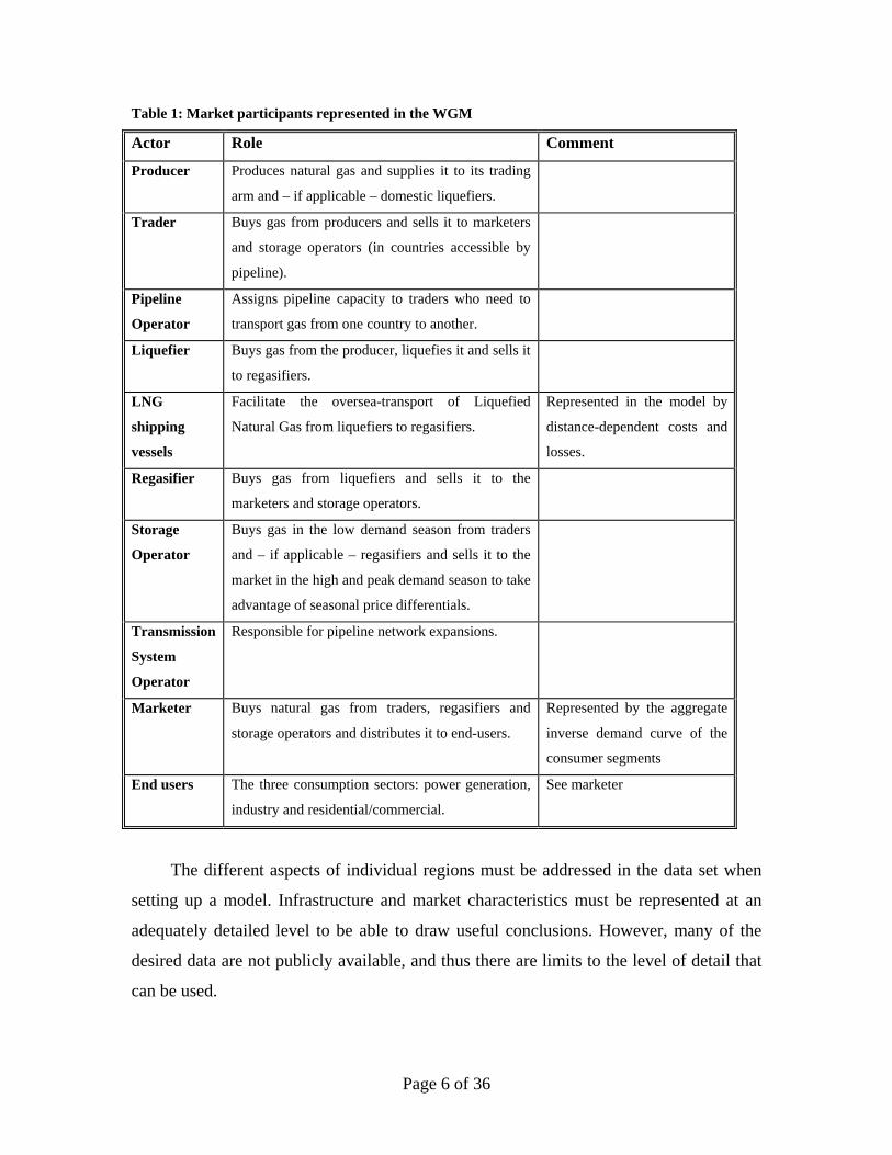
Table 1: Market participants represented in the WGM

Actor Role Comment

Producer Produces natural gas and supplies it to its trading

arm and – if applicable – domestic liquefiers.

Trader Buys gas from producers and sells it to marketers

and storage operators (in countries accessible by

pipeline).

Pipeline

Operator

Assigns pipeline capacity to traders who need to

transport gas from one country to another.

Liquefier Buys gas from the producer, liquefies it and sells it

to regasifiers.

LNG

shipping

vessels

Facilitate the oversea-transport of Liquefied

Natural Gas from liquefiers to regasifiers.

Represented in the model by

distance-dependent costs and

losses.

Regasifier Buys gas from liquefiers and sells it to the

marketers and storage operators.

Storage

Operator

Buys gas in the low demand season from traders

and – if applicable – regasifiers and sells it to the

market in the high and peak demand season to take

advantage of seasonal price differentials.

Transmission

System

Operator

Responsible for pipeline network expansions.

Marketer Buys natural gas from traders, regasifiers and

storage operators and distributes it to end-users.

Represented by the aggregate

inverse demand curve of the

consumer segments

End users The three consumption sectors: power generation,

industry and residential/commercial.

See marketer

The different aspects of individual regions must be addressed in the data set when

setting up a model. Infrastructure and market characteristics must be represented at an

adequately detailed level to be able to draw useful conclusions. However, many of the

desired data are not publicly available, and thus there are limits to the level of detail that

can be used.

Page 6 of 36

Figure 1 shows an overview of the – nearly 80 - countries and regions that are used

in the World Gas Model. For larger regions in Figure 1 the numbers in parentheses

indicate the number of sub-regions in the model. For example, the US consists of six

model nodes. Our data set covers 98% of the total production and consumption in 2005

(BP, 2008).

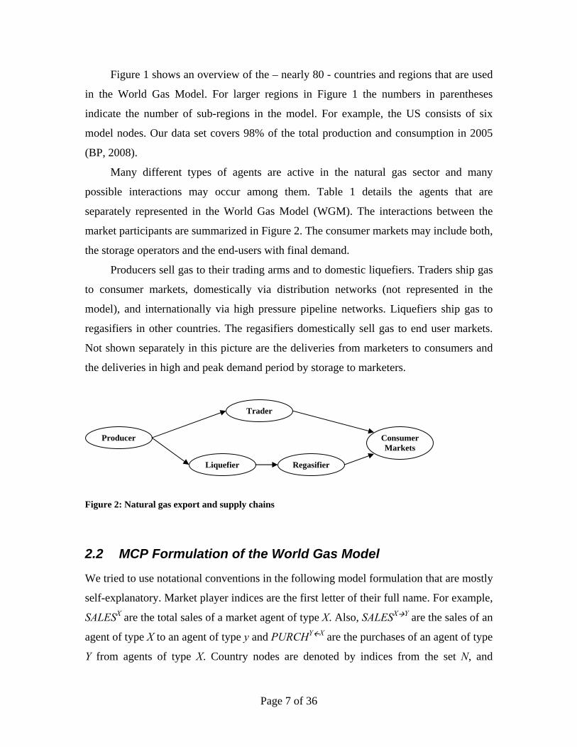
Many different types of agents are active in the natural gas sector and many

possible interactions may occur among them. Table 1 details the agents that are

separately represented in the World Gas Model (WGM). The interactions between the

market participants are summarized in Figure 2. The consumer markets may include both,

the storage operators and the end-users with final demand.

Producers sell gas to their trading arms and to domestic liquefiers. Traders ship gas

to consumer markets, domestically via distribution networks (not represented in the

model), and internationally via high pressure pipeline networks. Liquefiers ship gas to

regasifiers in other countries. The regasifiers domestically sell gas to end user markets.

Not shown separately in this picture are the deliveries from marketers to consumers and

the deliveries in high and peak demand period by storage to marketers.

Trader

Liquefier Regasifier

Consumer Markets

Producer

Figure 2: Natural gas export and supply chains

2.2 MCP Formulation of the World Gas Model

We tried to use notational conventions in the following model formulation that are mostly

self-explanatory. Market player indices are the first letter of their full name. For example,

SALESX are the total sales of a market agent of type X. Also, SALESXY are the sales of an

agent of type X to an agent of type y and PURCHYX are the purchases of an agent of type

Y from agents of type X. Country nodes are denoted by indices from the set N, and

Page 7 of 36

subsets of nodes where a player X is present, by N(x). To denote the subset of agents X

present at node n, we use: X(n). Where necessary and appropriate, more variable and

parameter names will be introduced. Greek letters are used the dual variables for

restrictions that are added in parentheses and will be used when deriving the KKTs.

2.2.1. Natural Gas Producers’ Problem

The production of natural gas includes the well operation and the processing of the

produced natural gas. We deal with the produced natural gas that is available for the

market, i.e., without so-called “own use” or re-injection into gas fields. We consider one

producer agent per production node (in general a country) that disposes of the aggregated

production capacities in that node and decides on total production.

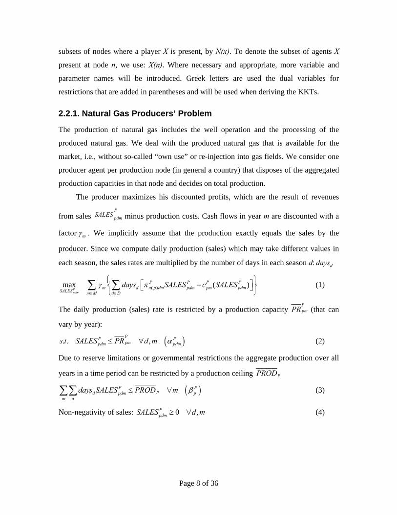
The producer maximizes his discounted profits, which are the result of revenues

from sales P

pdmSALES minus production costs. Cash flows in year m are discounted with a

factor m . We implicitly assume that the production exactly equals the sales by the

producer. Since we compute daily production (sales) which may take different values in

each season, the sales rates are multiplied by the number of days in each season d: ddays

( )max ( )Ppdm

P P P Pm d n p dm pdm pm pdm

SALES m M d D

days SALES c SALES

(1)

The daily production (sales) rate is restricted by a production capacity PpmPR (that can

vary by year):

. . ,PPpmpdm pdms t SALES PR d m P (2)

Due to reserve limitations or governmental restrictions the aggregate production over all

years in a time period can be restricted by a production ceiling pPROD

P Ppd pdm

m d

days SALES PROD m p (3)

Non-negativity of sales: (4) 0 ,PpdmSALES d m

Page 8 of 36

2.2.1.1 KKT conditions for the producer problem

To obtain the MCP model we take the first order conditions with respect to each decision

variable (here:P

pdmSALES ) of the profit maximization problem(s) to derive the Karush-

Kuhn-Tucker (KKT) conditions. The following are the KKT conditions for the producer

optimization problem which are necessary by the linearity constraint qualification and

sufficient as long as the production cost function ( )Ppmc is convex (Bazaara et al., 1993).

( )

( )

0 0

P Ppm pdmP

d m n p dm P Ppdm pdm

P Ppdm d p

c SALESdays

SALES SALES d m

days

, (5)

0P P Ppm pdm pdmPR SALES d m 0 , (6)

0 0

P Pp d pdm p

m d D

PROD days SALES

, ,

(7)

The market-clearing conditions, and the market-clearing price that tie the

producer optimization problem to the optimization problems of the traders and liquefiers

are as follows:

Pn p dm

2

( ) ( )( )

0 0P T P L P Ppdm t p n p dm ldm n p dm

l L p

SALES PURCH PURCH d p m

2.2.1.2 Production input data and supply cost function

While we use a generic convex production cost function in the above optimization

problem we detail our specific choice next. We assume a functional form following

Golombek et al. (1995), including a steep increase of production costs close to the

capacity limit Q.

C q ( )q 1

2q2 Q q ln Q q

Q

, 0, 0, 0,q : 0 q Q

2 In practice this inequality holds as an equality and should hold as shown in Zhuang (2005).

Page 9 of 36

for which the marginal supply cost curve is:

Q

qQqqC ln' and where Q is

the production capacity, is the minimum per unit cost term, the per unit linearly

increasing cost term, and a term that induces high marginal costs when production is

close to full capacity. To derive the parameters , and we set the production rate q

equal to the reference value of production in the base year.

2.2.2. Traders’ Problem

The traders in the WGM have a simplified role: they buy gas from one or more producers

and sell gas to one or more final consumption markets. Examples of traders in today’s

natural gas markets include Gazexport, the trading arm for Gazprom (Russia) and

GasTerra for NAM (Nederlandse Aardolie Maatschappij). This modeling approach can

represent both, a vertically integrated production and trading company (separate parts of

the same overall organization with marginal cost internal accounting prices) as well as an

independent trader that purchases gas from one or several producers. We distinguish two

types of traders:

A. Traders operating only at the domestic node of the producer in case it is a small

producer that does not export any gas. Previous papers (e.g., Boots et al., 2004)

usually refer to this production as exogenous production, and do not model these

quantities endogenously.

B. Traders that can operate at any consumption node that can be reached via

pipelines through transit nodes from their own producer’s node.

The trader maximizes profits resulting from selling gas to marketers ( ) and –

in the low demand season,

T MtndmSALES

1 lowd - to storage operators ( SA ), net of the gas

+purchasing costs and the costs of using the transportation system , a

regulated fee plus congestion fee, for the gas flow ( ) between ( . The

parameter

T Sm

i

Ann dm nn

, in n

tnLES

i

Ttnn dmW

i

Regdm

)FLO

, 0,1Ct n indicates the level of market power exerted by a trader t at a

Page 10 of 36

consumption node n; a value of 0 representing perfect competitive behavior and 1

Cournot (oligopolistic) behavior. The expression , ,(1 )C W C Wt n ndm t n ndm

Wnd

can be

viewed as a weighted average of market prices resulting from the inverse demand

function and a perfectly competitive market clearing wholesale price Wndm m .

)C W T Mndm tndm

Stnm

P T Ptndm

SALES

FLO

, ,

( )

( ( ))

(1

maxT Mtndm

T Stnm

Ttnn dmi

i iT Ptndm

C Wt n ndm t n

low T Td d ndm

d D n N t

n p t dmSALES

SALES

A RegFLOWd nn dm nn dm

PURCH

days SALES

PURCH

days

m

i

Ttnn dmW

( ), , TtndmN t d m

( , ) ( )id D n n A t

m M

)

T Ptndm

n n

H

loss

T MtndmES

0T Sm

T Ptndm

in dm

(8)

The following mass balance equation ensures that the volumes bought from the producer

and imported by pipeline must be enough to meet the total sales and the pipeline exports,

for each node in each season.

(1

i i

ii

i

low T Sd tnm

T MT tndm

tn ndmTn N

tnn dmn N

SALESPURCSALES nFLOW

FLOW

(9)

The remaining constraints enforce non-negativity of the decision variables:

s.t. SAL (10) 0 , ,n d m

,tnSALES n m (11)

0 ( ( )),PURCH n n p t d m , (12)

0 ( , ) ( ), ,Ttn iFLOW n n A t d m (13)

Beside traders, regasifiers ( ) and, in the high and peak demand seasons,

storage operators ( ) can sell gas to the marketers, too. Market clearing in the

end-user market, at a wholesale price

R MrdmSALES

Wndm

S MsdmSALES

, is enforced by the following inverse demand

function:

Page 11 of 36

( )

( )

( )

, ,

(1 )

T Mtndm

t T n

W M M R Mndm ndm ndm rdm ndm

r R n

low S Md sdm

s S n

SALES

INT SLP SALES n d m

SALES

W (14)

The market-clearing conditions between traders and storage operators in the low

demand (injection) season are as follows:

1( ) ( )

0 0T S S T Ttnm sm n m

t T n s S n

SALES PURCH n N t N s m

( ) ( ) ,

)L

(15)

KKT conditions for the trader and the following players’ optimization problems can be

found in the Appendix. They are derived in the same way as described above for the

producer, that is by taking the first-order conditions with respect to each decision variable

and including the constraints.

2.2.3. Liquefaction

In the model, export LNG terminals (“liquefiers”) are represented as players that buy gas

from a single producer (located in the same country node) and can sell it to regasifiers

around the world. The liquefier player in the World Gas Model covers the liquefaction

process including its internal optimization of LNG storage.

The LNG market today is characterized by a large amount of contracted sales that

imply that liquefiers have committed to sell a minimum amount of natural gas in general

to a specific LNG importing country (regasifier). Where available, we include the data

for contracts as a constraint in the model.3

The liquefier maximizes his discounted net profits from selling gas to regasifiers

, minus costs to purchase the gas and costs for liquefaction

and investment costs

LldmSALES

(Llmc SALES

L PldmPURCH

ldmL Llm lmb .

3 We thank Sophia Rüster and Anne Neumann for sharing the contract information from their data base.

Page 12 of 36

( )

( )

,

max

( )Lldm

L P Lldm lm

L Ln l dm ldm

P L P Lm d n l dm ldm lm

SALES m M d DL L

PURCHlm ldm

SALES

days PURCH b

c SALES

Llm (16)

Sales rates in any year are restricted by liquefaction capacity. Liquefaction capacity can

be expanded to be available in the following period. Therefore, the total liquefaction

capacity in a certain year m is the sum of the initial capacity L

lLQF and the expansion

investments in all former years ''

Llm

m m

.4

''

. . ,LL L

ldm lm ldmlm m

s t SALES LQF d m

L (17)

Liquefaction losses are significant and have to be accounted for in the mass balance

between purchases and sales:

(1 ) 0 ,L P L Ll ldm ldm ldmloss PURCH SALES d m (18)

There can be regulatory, technical or budget restrictions limiting the capacity expansions

in specific periods:

L L Llm lm lmm (19)

Non-negativity of the involved variables:

0 ,L PldmPURCH d m (20)

0 ,LldmSALES d m (21)

0Llm m (22)

The market-clearing conditions between liquefiers and regasifiers are as follows,

where the index b denotes the LNG tanker, running from node ns(b) to ne(b):

( )( ( )) : ( ) ( )

0 0s

L R L Lldm bdm n l dm

l L n l b n b n l

SALES PURCH d m

,

(23)

4 Capacity expansions cannot be executed instantaneously. Typically a multi-period run contains years that

represent every fifth year in the time horizon. Five years are generally enough for addressing the time lag

between a capacity expansion decision and the expansion to be constructed.

Page 13 of 36

2.2.4. Regasification

The following section describes the problem of the importing side in the liquefied natural

gas market, the regasification.. Regasifiers can buy gas from liquefiers and sell it to

domestic storage operators and to marketers. The regasifiers can exert market power

relative to the marketers, thereby representing strategic behavior on the LNG market,

similar to the traders for the pipeline market.

Contrary to liquefiers, we may include more than one regasifier in a country

depending on the country’s geography. This choice allows countries like Spain, France

and Mexico to have LNG import capacity on their respective East and West coasts,

thereby potentially providing interesting insights in the developments in the various

global basins.5

The operational process of a regasifier includes the internal optimization of LNG

storage in addition to the main activities of unloading the LNG vessels and bringing the

vaporized (gaseous) natural gas into the pipeline system. Moreover, in the WGM the

regasifier’s problem includes the optimization of LNG shipment by tankers. It is

represented by a distance-based shipping cost and a gas loss rate that allow the regasifier

to determine the optimal transport from any liquefier.

The regasifier maximizes his discounted profits resulting from the sales to

marketers and storage operators minus the costs to purchase and

ship the gas

R MrdmSALES R S

rdmSALES

R LbdmRCH ( )s

L R Ln b dm bu PU

Rrmb

( )R Srdm

, the re-gasification costs

and investment costs R R Mrdm SALES rmc SALES R

rm .

5 However, our simplified representation does not allow for representing recent developments such as co-

ownerships of LNG terminals such as the majority share of the French company GDF Suez and minority

shares of Italian Publigas and others in the Belgian Zeebrugge terminal.

Page 14 of 36

( )

,( )

: ( ) ( )

(1 )

max

( )

R Mrdm

sR Srdm e

R Lbdm

Rrm

C W C W R Mr ndm r ndm rdm

R R Sn r dm rdm

R Rm d rm rmL R L R L

SALES d D n b dm b bdmSALES b n b n r

PURCH R R M R Srm rdm rdm

SALES

SALESdays b

u PURCH

c SALES SALES

m M

(24)

Sales (i.e, regasification) rates in any year are restricted by the regasification capacity.

Regasification capacity can be expanded by an endogenous investment decision. Hence,

the total capacity in a certain year m is the sum of initial capacity RrREG and the yearly

expansions in previous years, ''

Rrm

m m

.

''

. .

,RR M R S R Rrrdm rdm rm rdm

m m

s t

SALES SALES REG d m

(25)

The purchased gas, corrected for shipment losses ( ) and regasification losses ( ),

must be greater or equal to the total sales:

bloss rloss

: ( ) ( )

(1 )(1 ) 0 ,e

R MrdmR L R

r b bdm rdmR Sb n b n r rdm

SALESloss loss PURCH d m

SALES

(26)

Again, there can be regulatory, technical or budget restrictions limiting the capacity

expansions in specific periods:

( )R R Rrm ry m rmm (27)

The presence of contracts may impose a lower bound on purchases from a specific

liquefier in a certain year:

( ) : ( ) ( ), ,R L R Rbdm bdy m e bdmPURCH Contract b n b n r d m (28)

Non-negativity of the decision variables:

0 ,R MrdmSALES d m (29)

0 1R SrdmSALES d m , (30)

0 : ( ) ( ), ,R Lbdm ePURCH b n b n r d m (31)

0Rrm m (32)

Page 15 of 36

The market-clearing conditions between regasifiers and storage operators are as follows:

1( ) ( )

0 0R S S R Rr m sm n m

r R n s S n

SALES PURCH n m

1 , (33)

2.2.5. Storage

Natural gas storage can be used for a variety of reasons, including daily balancing and

price arbitrage, seasonal balancing and as a strategic backup supply to overcome

temporary supply disruptions or to meet peak demand on cold winter days. We focus on

the seasonal arbitrage and assume the storage to be empty at the beginning and the end of

each year. Storage can also be used to compensate disrupted supplies in our model.

There are various types of gas storages: depleted reservoirs in oil and gas fields,

aquifers, and salt caverns. Each of them has different characteristics relative to the

amount of gas that can be stored and the speed with which the gas can be injected and

extracted. In most countries, one type of storage is prevailing and we include these

country-specific characteristics.

The amount of gas available for operation is the working gas. Typically, gas

installations have minimum and maximum injection and extraction rates. Compressors

are used to generate pressure to be able to inject the gas in the storage. These

compressors use some of the gas, therefore there is a loss rate associated with the

operations. In the WGM, we assume that storage operators buy gas and inject it in the

low demand season and extract gas and sell it in the high and peak demand seasons, as

long as the seasonal price differential (corrected for the loss rate) is larger than the

operational costs.

The storage operator sells gas to the domestic marketer in the high and peak

demand season: . The gas is bought in the low demand season (of that same

year) and injected into storage. Costs are made for purchasing the gas from the traders

and regasifiers , and to inject the gas into storage

. To expand capacity for injection, extraction or total

working gas, the investment costs sum up to .

S MsdmSALES

( TsmPURCH

S TsmPURCH

S Ssm sc PURCH

S RsmPURCH

)S Rm

, , , , , ,S INJ S INJ S EXT S EXT S WG S WGsm sm sm sm sm smb b b

Page 16 of 36

,

,

,

( )2,3

( )1

1 ( )1

, , ,

max

( )

S Tsm

S Rsm

S Msdm

S INJsm

S EXTsm

S WGsm

W S Md n s dm sdm

d

T S Tn s m sm

R S Rm n s m sm

PURCHS S T S

PURCHsm sm sm

SALESS INJ S INJ S EXTsm sm sm s

days SALES

PURCH

days PURCH

c PURCH PURCH

b b

, , ,

m M

S EXT S WG S WGm sm smb

R

(34)

Injection rates in any year are restricted by the injection capacity. Capacity can be

expanded, therefore the total capacity in a year is the sum of initial capacity SsINJ and the

yearly expansions . Similar explanations apply to ,'

'

S INJsm

m m

(36) and (37) for extraction

and working gas limitations.

,'

'

. .SS T S R S INJ Ss sm sm sm

m m

s t

PURCH PURCH INJ m sm

(35)

,'

'

2,3,SS M S EXT Sssdm sm sdm

m m

SALES EXT d m

(36)

,'

2,3 '

SS M S WG Ssd sdm sm

d m m

days SALES WRKG m sm

(37)

Total purchases corrected for losses must be enough to cover the total sales:

12,3

(1 ) 0S Tsm S M S

s d sdmS Rdsm

PURCHdays loss days SALES m

PURCHsm

(38)

Limitations to the capacity expansions:

, , ,( )

S INJ S INJ S INJsm sy m smm (39)

, , ,( )

S EXT S EXT S EXTsm sy m smm (40)

, , ,( )

S WG S WG S WGsm sy m smm

,

))

(41)

Non-negativity of the decision variables:

0 2,3S MsdmSALES d m (42)

0 , ( (S TsmPURCH m t T s n (43)

Page 17 of 36

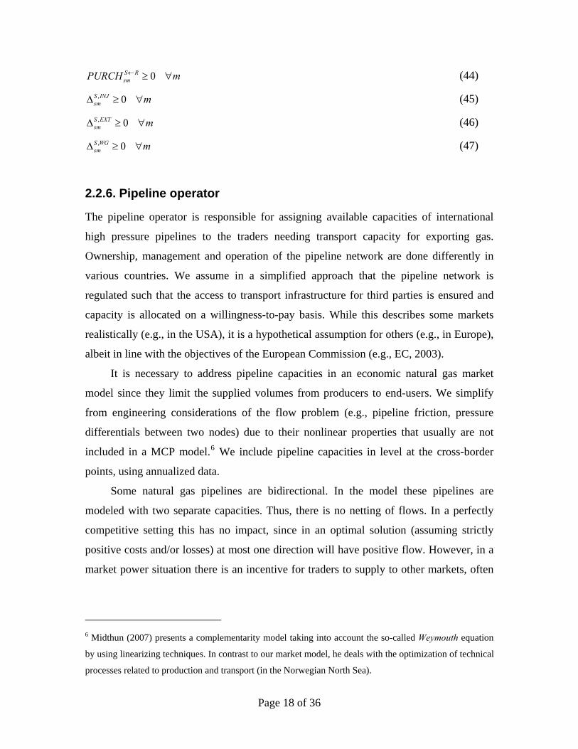
0S RsmPURCH m (44)

, 0S INJsm m (45)

, 0S EXTsm m (46)

, 0S WGsm m (47)

2.2.6. Pipeline operator

The pipeline operator is responsible for assigning available capacities of international

high pressure pipelines to the traders needing transport capacity for exporting gas.

Ownership, management and operation of the pipeline network are done differently in

various countries. We assume in a simplified approach that the pipeline network is

regulated such that the access to transport infrastructure for third parties is ensured and

capacity is allocated on a willingness-to-pay basis. While this describes some markets

realistically (e.g., in the USA), it is a hypothetical assumption for others (e.g., in Europe),

albeit in line with the objectives of the European Commission (e.g., EC, 2003).

It is necessary to address pipeline capacities in an economic natural gas market

model since they limit the supplied volumes from producers to end-users. We simplify

from engineering considerations of the flow problem (e.g., pipeline friction, pressure

differentials between two nodes) due to their nonlinear properties that usually are not

included in a MCP model.6 We include pipeline capacities in level at the cross-border

points, using annualized data.

Some natural gas pipelines are bidirectional. In the model these pipelines are

modeled with two separate capacities. Thus, there is no netting of flows. In a perfectly

competitive setting this has no impact, since in an optimal solution (assuming strictly

positive costs and/or losses) at most one direction will have positive flow. However, in a

market power situation there is an incentive for traders to supply to other markets, often

6 Midthun (2007) presents a complementarity model taking into account the so-called Weymouth equation

by using linearizing techniques. In contrast to our market model, he deals with the optimization of technical

processes related to production and transport (in the Norwegian North Sea).

Page 18 of 36

resulting in congested pipelines in both directions (see Egging and Gabriel, 2006, for a

deeper analysis of this issue).

The pipeline operator provides an economic mechanism to efficiently allocate

pipeline capacity to traders. The pipeline operator maximizes the discounted profit

resulting from selling pipeline capacity to traders, . The regulated fees

collected from the traders are assumed to equal the operating costs, therefore the profit

margin is equal to the congestion fee .

i

Ann dmSALES

i

Ann dm

( , )

maxA inn dmi i

A Am d nn dm nn dm

SALES m M n n d D

days SALES

i

(48)

The assigned pipeline capacity can be at most the available capacity. Available pipeline

capacity on an arc (n,ni) is the sum of initial pipeline capacity i

AnnPL and capacity

expansions in former years . ''

i

Onn m

m m

''

. .

,ii i

AA Onnnn dm nn m nn dm

m m

s t

SALES PL d m

i

A

( , ), ,

(49)

Non-negativity of variables:

0 ,i

Ann dmSALES d m (50)

Market-clearing conditions for pipeline capacity between pipeline operator and traders:

(( , ))

0 0i i i

i

A T Ann dm tnn dm nn dm i

t T n n

SALES FLOW n n d m

(51)

2.2.7. Transmission System Operator Problem

The market agent that we assume to be responsible for expanding the pipeline network is

the transmission system operator (TSO). The transmission system operator maximizes a

function with revenues from congestion payments and investment costs of expansion of

the pipeline network. This mechanism balances the pipeline investment costs and the

added value to the market given by the added pipeline capacity. Hence, we represent the

long-term optimization of the pipeline network.

Page 19 of 36

The separation of short-term and long-term optimization ensures that there is no incentive

to withhold long-term capacity expansion in order to increase congestion revenues in the

short-term. However, given that the endogenous variables from one player (TSO) enter

into the optimization problem (in the constraint set) of another player (the pipeline

operator), this version of the World Gas Model is in fact an instance of a generalized

Nash problem. As such, it is equivalent to a quasi-variational inequality. Under certain

circumstances, one can solve an associated variational inequality (or mixed

complementarity) problem to resolve it, as we do here. The optimization problem of the

transmission system operator is given as follows:

'( , ) ' ( , )

max

O i i i i

nn mi i i

A O O Om d nn dm nn m nn m nn m

m M n n d D m m n n

days b

(52)

There may be limitations to the allowable pipeline expansions

. .

, ,i i i

O O Onn m nn m i nn m

s t

n n m (53)

Non-negativity of the expansion decision variables

0 , ,i

Onn m in n m (54)

2.2.8. Marketer, Distribution and Consumption Sectors

The KKT and market-clearing conditions presented in the above sections represent the

World Gas Model. Some market aspects are indirectly accounted for in the model. The

main one is the final consumption by three sectors (electricity generation, industry,

residential) that are represented via an aggregation of their respective inverse demand

functions into a single inverse demand function, which in turn represents the marketer.

For our analysis of the world gas market and the international trade flows, it is not

necessary to include all different demand sectors in each country. Equation (14) in the

trader problem (Section 2.2.2) shows the aggregate demand function. To simplify the

model structure and limit the number of model variables, we include country aggregate

inverse demand curves. However, the model is calibrated by sector level and the sector

Page 20 of 36

level information is retained. Ex-post the demand for each sector can be calculated based

on the individual inverse demand curves. As long as all sectors have positive

consumption, we know that the aggregation to a single inverse demand curve does not

change the obtained outcomes compared to sector-specific demand functions.

The combination of all KKTs and the market-clearing conditions form the market

equilibrium (MCP) model. Due to concavity of the profit functions7, convexity of the

cost functions and convexity of the feasible regions, the KKT points for this system are

optimal solutions.

3 Data Set

We are interested in the international trade of natural gas, so most countries are

represented as just one node. Large countries and/or countries active in several regional

basins are split up into several nodes, such as the U.S.A., Canada, Russia, and Mexico.

We deal with normalized units of natural gas (at 15°C temperature and 760 mmHG

pressure as defined by the International Energy Agency, e.g., IEA, 2008a). The data set

can be adapted for scenario runs (e.g., Huppmann et al., 2009); here we present the base

case data set and assumptions. Our base year is 2005 and we need additional data input

for the following model years 2010, 2015, 2020, 2025, 2030, 2035 and 2040. 8 We

assume a 10% discount rate in the multi-period optimization. In general, we use data per

day, distinguished by season (low, high and peak demand) where applicable.

On the supply side, we must realistically include limits on how much can be

produced and transported. These capacity constraints are based on existing facilities for

the base year and include projects currently under construction for the second model

period (2010).9 Starting in 2010, there can be endogenous investments in transport and

storage infrastructure. In order to maintain a MCP we assume continuous capacity

7 Since we are minimizing the negative of a concave profit function, we are effectively minimizing a

convex function. 8 The last two model years are not reported in the model results, but they are necessary to have a sufficient

payback period for the model-derived, endogenous investments. 9 We also include one exogenous reduction of capacity in 2015, namely the LNG terminal in Alaska which

will cease operations by 2012.

Page 21 of 36

expansions. The investment is limited in each period; where available we use projections

to determine these limits, otherwise we include our own assessment.

Production capacity data for the base year is based on information and forecasts in

the technical literature (e.g., OME, 2005, Oil and Gas Journal). Production capacity is

determined exogenously for all model periods (i.e., no endogenous investments). For

future periods, we apply a growth rate to the base year capacity that is based on

production growth projections with the PRIMES model for Europe (EC, 2008) and the

POLES model for the rest of the world (EC, 2006).

International pipeline transport is limited at the cross-border points. When there are

several cross-border points between two adjacent country nodes, we aggregate the

capacities of these points to a single bound. We use capacity data from GTE (2005, 2008)

for intra-European transport. Data on pipeline capacity between the North American

nodes10 was obtained from the Energy Information Agency. For all other pipelines, we

use company reports and websites as well as technical literature. For given pipeline

expansions between 2005 (first model period) and 2008 (time of our data base

construction), we exogenously include the realized capacities in the model year 2010.

For new greenfield pipeline projects that are planned but do not exist yet, e.g. the

Nabucco pipeline, we include a zero capacity in the first model year and allow for

positive investments in later periods (with the exact period depending on the project).

Storage capacities are obtained from IEA (2007) and GSE (2008) for existing facilities.

GSE (2008) also provides projected capacities in Europe.

The LNG transport value chain contains liquefaction, shipment and regasification,

as explained above. Liquefaction and regasification capacity data for 2005 are from IEA

(2007). For future capacity expansion limits, including new terminals, we use technical

literature such as IEA (2008b), the Oil and Gas Journal, etc. For the downstream actor in

the LNG chain, the regasifier, we additionally use GLE (2005) for Europe. Shipment is

optimized by the regasifier, given the distance-based transport costs. Distances between

each pair of liquefier and regasifier are obtained for the approximate location of the

10 North America is split into nine regions: Alaska, Canada-East and Canada-West, US-West, US-Rockies,

US-Gulf, US-Midwest, US-East, and Mexico.

Page 22 of 36

terminals using www.distances.com. There is no restriction on the trading pairs, and we

do not include limits on the shipment capacity.

We assume linear cost functions for the construction of incremental capacity of

transport or storage. The parameters are averages based on reported project costs in

technical literature such the Oil and Gas Journal and company information. In the LNG

value chain, the parameters are chosen such as to reflect the fact that the infrastructure for

the regasification of gas is less capital intensive than the liquefaction. For pipelines, we

determine a base cost of 50,000,000 US-$ for a new capacity of 1 bcm/year between two

nodes, based on industry cost reports. For each of the characteristics “greenfield project”,

“very long pipeline” or “offshore pipeline”, this unit cost is doubled.

Storage expansions comprise expansion of injection, extraction and working gas

capacity. Building extra injection capacity is costlier (our assumption: 3,000,000 US-

$/mcm/d) than building extra extraction (500,000 US-$/mcm/d). For working gas the

investment costs are 150,000 US-$/bcm.

Short-run production costs and losses are similar to Egging et al. (2008) but have

been updated. As explained in the model description above, the production cost function

in the short term is a function of the produced quantity that increases strongly close to the

production capacity limit (Golombek et al., 1995). The parameters for the cost function

are derived from OME (2005) but had to be adjusted upwards in the calibration process.

Short-term transport costs per pipeline are a linear function, related to the distance

to be traveled and including royalties where applicable (e.g. for the pipeline through

Tunisia). Similarly, losses for pipeline transportation are assumed to be higher for long-

distance pipelines, following Oostvoorn (2003). For LNG transport, we apply linear cost

functions for liquefaction and for regasification. In the absence of detailed data, we use

the same parameters for all countries. Shipment costs and losses, that are added to the

regasification costs, are distance-based.

The total demand function for natural gas is obtained from aggregating sector-

specific consumption for each country. The International Energy Agency, in its Monthly

Natural Gas Survey (http://www.iea.org/Textbase/stats/surveys/archives.asp) reports

consumption levels for the power sector, industry, residential/households and other

categories for each month. We aggregate these data by season (low, high and peak

Page 23 of 36

demand), with the monthly distribution depending on the geographic location of each

country (with differences, e.g., between the Northern and the Southern hemisphere) and

determine a parameter reflecting the intensity of seasonal change of demand. For each

sector-specific demand, another price elasticity is assumed (between -0.25 and -0.75). For

the construction of the demand function for each period, we also need a reference price.

The 2005 prices are based on IEA (2007) and BP (2008). For future periods, we assume

an annual growth rate in the willingness to pay of 3%, based on EC (2008). Total demand

is then an aggregated function of the linear functions for each sector.

4 Base Case Results

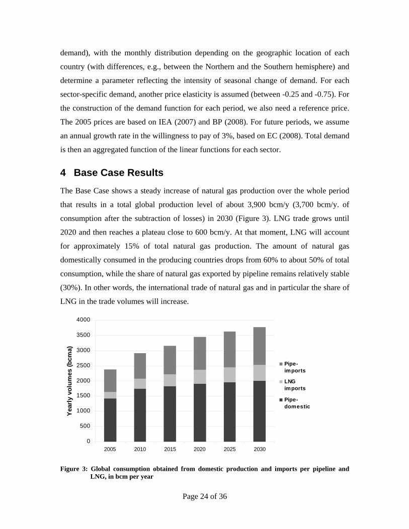
The Base Case shows a steady increase of natural gas production over the whole period

that results in a total global production level of about 3,900 bcm/y (3,700 bcm/y. of

consumption after the subtraction of losses) in 2030 (Figure 3). LNG trade grows until

2020 and then reaches a plateau close to 600 bcm/y. At that moment, LNG will account

for approximately 15% of total natural gas production. The amount of natural gas

domestically consumed in the producing countries drops from 60% to about 50% of total

consumption, while the share of natural gas exported by pipeline remains relatively stable

(30%). In other words, the international trade of natural gas and in particular the share of

LNG in the trade volumes will increase.

0

500

1000

1500

2000

2500

3000

3500

4000

2005 2010 2015 2020 2025 2030

Yea

rly

volu

mes

(b

cma)

Pipe-imports

LNGimports

Pipe-domestic

Figure 3: Global consumption obtained from domestic production and imports per pipeline and LNG, in bcm per year

Page 24 of 36

$0

$100

$200

$300

$400

$500

$600

2005 2010 2015 2020 2025 2030

0%

20%

40%

60%

80%

100%

120%

140%

160%

180%

PriceEurope

PriceNorthAmerica

RelativeEurope

RelativeNorthAmerica

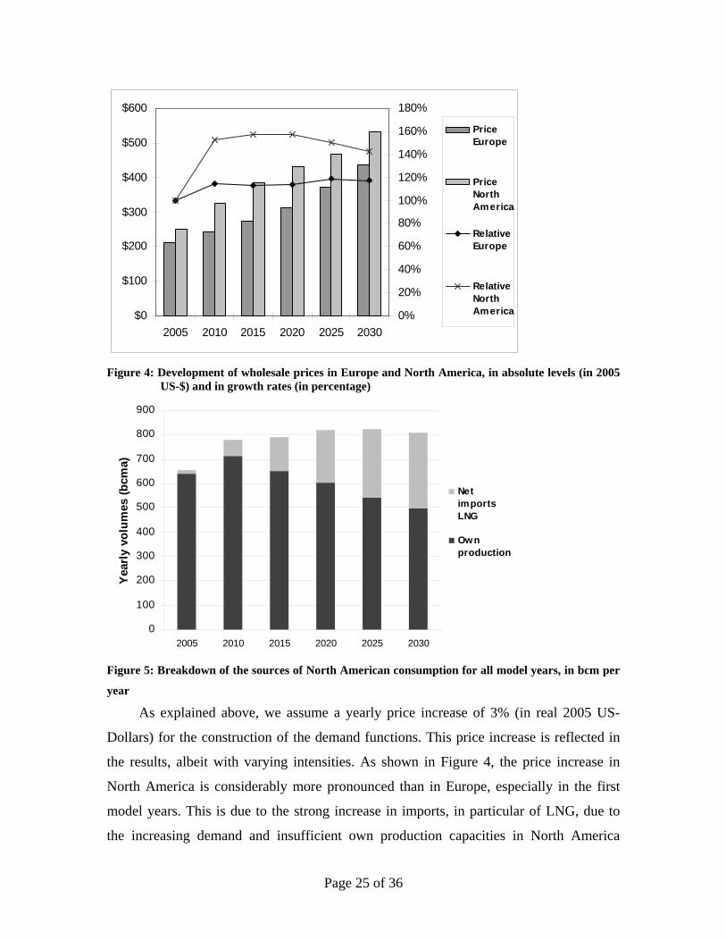
Figure 4: Development of wholesale prices in Europe and North America, in absolute levels (in 2005

US-$) and in growth rates (in percentage)

0

100

200

300

400

500

600

700

800

900

2005 2010 2015 2020 2025 2030

Yea

rly

volu

mes

(b

cma)

NetimportsLNG

Ownproduction

Figure 5: Breakdown of the sources of North American consumption for all model years, in bcm per

year

As explained above, we assume a yearly price increase of 3% (in real 2005 US-

Dollars) for the construction of the demand functions. This price increase is reflected in

the results, albeit with varying intensities. As shown in Figure 4, the price increase in

North America is considerably more pronounced than in Europe, especially in the first

model years. This is due to the strong increase in imports, in particular of LNG, due to

the increasing demand and insufficient own production capacities in North America

Page 25 of 36

before alternative domestic supply sources (from Alaska) come on-stream (Figure 5).11 In

2030, North America produces about 60% of its consumption domestically with the

remaining 40% satisfied by LNG imports.

In 2030, the Middle East, Russia and the Caspian region split the major part of

their sales between Europe and Asia, with small amounts sold as LNG to North America.

Total consumption in Europe in 2030 amounts to 667 bcm/y.; of this, 27 bcm/y. are

supplied in the form of LNG, which accounts for 4% of total consumption, and 200

bcm/y. are produced domestically. A large share of European consumption is imported

from Russia and the Caspian region, but also from North Africa as pipeline gas (Figure

6). Hence, in the competition for LNG in the Atlantic basin, North America would be

able to take the lead because of its higher willingness to pay in the absence of other local

sources. Europe, in contrast, can continue to rely on a number of pipeline import options

with LNG playing the role of marginal supplier with important diversification impacts.

0

100

200

300

400

500

600

700

800

2005 2010 2015 2020 2025 2030

Yea

rly

volu

mes

(b

cma)

NetimportsLNG

Netimportspipe

Ownproduction

Figure 6: Breakdown of European consumption for all model years, in bcm/y.

11 The Base Case does not include unconventional resources that have recently been added to the North American reserves. We explore the impact of the large increase in North American production capacities that may result from shale gas production in a scenario in Huppmann et al. (2009). and Gabriel, S.A., R. Egging, H. Avetisyan, “An Analysis of the North American Natural Gas Market Using the World Gas Model.” (working title, forthcoming).

“

Page 26 of 36

Asia consumes almost 850 bcm/y. in 2030 with Japan and Taiwan continuing to

rely heavily on LNG imports that come to a large extent from the Middle East. China and

India each produce half of their consumption domestically and import another 40% by

pipeline from Russia, Myanmar, and the Caspian region.

Liquefaction and regasification capacities over time are shown in Figure 7. While

liquefaction capacities increase from 242 bcm in 2005 to 652 bcm/y. in 2030,

regasification capacities expand even further from 491 to 945 bcm/y. Thus, we continue

to observe proportionally higher regasification capacity than liquefaction capacity

reflecting the flexible spot LNG trade that we assume at least for later model runs. There

are certain spare capacities in order to meet seasonal demand or to benefit from the

option of importing additional volumes of liquefied natural gas. Investment in LNG

infrastructure is strongest at the beginning of the time horizon (where it is to some extent

driven by the inclusion of projects currently under construction) and again in 2020. After

2020, investments slow down due to the assumption of demand stagnation in many

developed markets.

0 50 100 150 200 250 300 350 400 450 500

Africa

Australia

Asia

North America

Europe

Latin America

M iddle East

Russia West

Russia East current liquefaction

liquefaction 2030

current regasification

regasification 2030

Figure 7: Liquefaction and regasification capacities; in bcm/y.

The pipeline capacity development is reported in Table 2 for those regions where pipeline

trade plays an important role. One can see that Russia as well as the Caspian and the

Middle Eastern regions are considerably expanding their pipeline capacities to Asia, in

Page 27 of 36

particular after 2015, in many places with construction of new, greenfield pipeline

projects. These new pipeline capacities can accommodate the large exports of natural gas

to satisfy the strong Asian demand for natural gas. Europe continues to be an important

pipeline market with decreasing domestic production and a stable demand for natural gas.

In line with the minor role for LNG on the European market, some substantial pipeline

capacity expansions are coming forward: above all from North Africa, but also from the

Caspian region and the Middle East.

Table 2: Pipeline capacities over time between selected world regions, in bcm/y.

Incoming

Outgoing Year Europe

Ukraine,

Belarus Caspian Middle East Asia-Pacific

Africa 2005 49

2015 92

2030 130

Ukraine, Be- 2005 208 29

larus 2015 212 29

2030 213 29

RUSSIA 2005 40 207 13 0

2015 87 230 13 0

2030 183 233 13 91

Caspian 2005 7 118 8 0

2015 25 215 45 33

2030 52 247 45 117

Middle East 2005 10 0 2 0

2015 26 2 6 0

2030 54 2 6 38

Asia-Pacific 2005 20

2015 44

2030 148

5 Conclusions

We have presented an extensive model of the global natural gas markets, the flows and

the infrastructure, called the World Gas Model. This multi-period model allows to take

Page 28 of 36

into account endogenous investment decisions over the next decades while at the same

time including market power in the pipeline and the LNG market.

Our Base Case results confirm the results by larger energy system models and

exhibit an increase in global natural gas trade in the next decades. However, the strong

rise, in particular of LNG trade will not be sustained after 2020. The largest increase in

natural gas consumption and imports will come from Asia where, consequently, the

biggest expansion of infrastructure capacity takes place.

The World Gas Model can be used for a variety of analyses of trends in the

international natural gas and energy markets. In Huppmann et al. (2009) we presented

several development scenarios until 2030, including such intriguing questions as the

unconventional resource base in the U.S. which may trigger considerably less LNG

demand and the advent of an alternative “clean technology” that would gradually replace

natural gas.

In Egging et al. (2009) we discussed the possibility and effects of a cartelization of

the natural gas markets within the Gas Exporting Countries Forum. A simplifying

representation of the cartel was achieved by modifying the model structure in order to

incorporate a single trader of pipeline gas and a single LNG supplier for the cartel

countries.

Another extension of the model is the inclusion of stochastic aspects, that is to

allow for several scenarios to realize with a certain probability. In such a model, the

optimal reaction by the players is different to deterministic simulations because they have

to prepare for all possible events. For example, a pipeline from Iran to Europe may be

necessary in the future or not, depending on whether Iran and the Gas Exporting

Countries Forum will be able to implement an effective cartel withholding strategy. If the

probability of such a cartel is less than 100% it may still be optimal to built a pipeline,

maybe with a smaller capacity, in case the Iranian gas will not be withheld. Some first

stochastic WGM results are presented in Egging and Holz (2009) which complement the

work in Gabriel et al. (2009) for scenario reduction methods applied to small natural gas

networks.

Page 29 of 36

6 References

Bazaraa, M.S., H.D. Sherali, and C.M. Shetty, 1993. Nonlinear Programming Theory and

Algorithms. Wiley, New York.

Boots, M., Rijkers, F.A.M., Hobbs, B.F., 2004. A two-level oligopoly analysis of the

European gas market. The Energy Journal. Vol. 25, No. 3, pp. 73–102.

BP, 2008. Statistical Review of World Energy. London.

Cottle, R., J.S. Pang, and R. E. Stone, 1992. The Linear Complementarity Problem.

Academic Press.

EC, 2003. Directive 2003/55/EC Concerning Common Rules for the Internal Market in

Natural Gas. Official Journal, L 176 , 15/07/2003, pp. 57-78.

EC, 2006. World Energy Technology Outlook - 2050 (WETO-H2). European

Commission, Brussels.

EC, 2008: European Energy and Transport: Trends to 2030 - Update 2007. European

Commission, Brussels.

Egging, R. and S.A. Gabriel, 2006. “Examining market power in the European natural

gas market”, Energy Policy, Vol. 34, No. 17, pp. 2762-2778.

Egging, R., S.A. Gabriel, F. Holz, and J. Zhuang, 2008. “A Complementarity Model for

the European Natural Gas Market”. Energy Policy, Vol. 36, No. 7, pp. 2385-414.

Egging, R., F. Holz, S.A. Gabriel, and C. von Hirschhausen, 2009. “Representing Gaspec

with the World Gas Model”, The Energy Journal, Vol. 30, Special Issue: “World

Natural Gas Markets and Trade: A Multi-Modeling Perspective”, pp. 97-117.

Egging, R. and F. Holz, 2009. “Timing of Investments in an Uncertain World”.

Presentation at the 8th Conference on Applied Infrastructure Research (INFRADAY),

Berlin, October 2009.

Gabriel, S.A., S. Kiet, and J. Zhuang, 2005a. "A Mixed Complementarity-Based

Equilibrium Model of Natural Gas Markets", Operations Research, Vol. 53, No. 5,

pp. 799-818.

Gabriel, S.A., J. Zhuang, and S. Kiet, 2005b. "A Large-Scale Complementarity Model of

the North American Natural Gas Market", Energy Economics, Vol. 27, No. 4, pp.

639-665.

Page 30 of 36

Gabriel ,S.A., J. Zhuang, and R. Egging, 2009. “Solving Stochastic Complementarity

Problems in Energy Market Modeling Using Scenario Reduction,” European Journal

of Operational Research, Vol. 197, No. 3, pp. 1028-1040.

GLE, 2005. “Gas LNG Europe Map”. Brussels, 2005.

Golombek, R, E. Gjelsvik, and K.E. Rosendahl, 1995. “Effects of Liberalizing the

Natural Gas Markets in Western Europe”, Energy Journal, Vol. 16, No. 1, p. 85-111.

GTE, 2005. “Capacities of Cross-Border Points on the Primary Market”. Gas

Transmission Europe, Brussels, December 2005.

GTE, 2008. “Capacities of Cross-Border Points on the Primary Market”. Gas

Transmission Europe, Brussels, June 2008.

Holz, F., C. von Hirschhausen, and C. Kemfert, 2008. “A Strategic Model of European

Gas Supply (GASMOD)”. Energy Economics, Vol. 30, No. 3, pp. 766-88.

Huppmann, D. and R. Egging. User Manual, Functional and Technical Documentation

for the World Gas Model. Mimeo.

Huppmann, D., F. Holz, C. von Hirschhausen, S. Ruester, R. Egging, and S.A. Gabriel,

2009. “The World Gas Market in 2030 – Development Scenarios Using the World

Gas Model”, DIW Discussion Paper 931.

IEA, 2007. Natural Gas Information. OECD / International Energy Agency, Paris.

IEA, 2008a. Natural Gas Information. OECD / International Energy Agency, Paris.

IEA, 2008b. Natural Gas Market Review. OECD / International Energy Agency, Paris.

Lise, W. and B.F. Hobbs, 2008. “Future Evolution of the Liberalised European Gas

Market: Simulation Results with a Dynamic Model”, Energy, Vol. 33, No. 7, pp. 989-

1004

Midthun, K.T., 2007. Optimization Models for Liberalized Natural Gas Markets. Thesis,

Norwegian University of Science and Technology.

Oostvoorn, F.v., 2003. Long-Term Gas Supply Security in an Enlarged Europe. Final

Report ENGAGED Project. Petten, ECN.

Zhuang, J., 2005. A Stochastic Equilibrium Model for the North American Natural Gas

Market. PhD Dissertation. University of Maryland, Department of Civil and

Environmental Engineering.

Page 31 of 36

Zwart, G., 2009. “European Natural Gas Markets: Resource Constraints and Market

Power”. The Energy Journal, Vol. 30, Special Issue: “World Natural Gas Markets

and Trade: A Multi-Modeling Perspective”, pp. 151-65.

Page 32 of 36

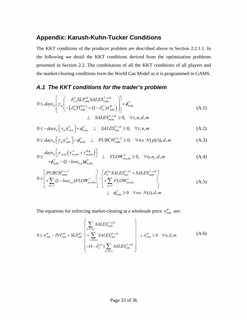
Appendix: Karush-Kuhn-Tucker Conditions

The KKT conditions of the producer problem are described above in Section 2.2.1.1. In

the following we detail the KKT conditions derived from the optimization problems

presented in Section 2.2. The combination of all the KKT conditions of all players and

the market-clearing conditions form the World Gas Model as it is programmed in GAMS.

A.1 The KKT conditions for the trader’s problem

,

( )0

(1 )

0, , , ,

C M T Mt n ndm tndm T

d m tndmC W T C Wtn ndm tn ndm

T Mtndm

SLP SALESdays

SALES t n d m

(A.1)

1 10 T T T Sd m n m tn m tnmdays SALES t n m 0, , ,

, ( ( )), ,

, , , ,

,

(A.2)

0 0P T T Pd m ndm tndm tndmdays PURCH n N p t d m (A.3)

( )0 0

(1 )

i i

i

i i

A Regd y m nn dm nn dm T

tnn dm iT Ttndm n n tn dm

daysFLOW n n d m

loss

(A.4)

0 (1 )

0 ( ),

i i i

i i

T P low T S T Mtndm d tnm tndm

T Tn n tn ndm tnn dm

n N n N

Ttndm

PURCH SALES SALES

loss FLOW FLOW

n N t d m

(A.5)

The equations for enforcing market-clearing at a wholesale price Wndm are:

( )

( )

( )

0 0

(1 )

T Mtndm

t T n

W M M R M Wndm ndm ndm rdm ndm

r R n

low S Md sdm

s S n

SALES

INT SLP SALES n d m

SALES

, , (A.6)

Page 33 of 36

A.2 KKT conditions for the liquefier optimization problem

( )

( )0

0 ,

L LL Llm ldm

d m n l dm ldm ldmLldm

Lldm

c SALESdays

SALES

SALES d m

L

0 m

(A.7)

( ) ''

0

L L L Lm ly m ldm lm lm

d D m m

b (A.8)

''

0L L L L

lm ldm ldmlm m

LQF SALES d m

0 , (A.9)

0 (1 ) 0 ,L P L Ll ldm ldm ldmloss PURCH SALES d m (A.10)

0 L L Llm lm lm m 0 (A.11)

A.3 KKT conditions for the regasifier problem

( )( )0 (1 )

( )

0, ,

C M R Mr ndm rdm

C W T C W R Rd m r ndm r n r dm rdm rdm

R R M R Srm rdm rdm

R Mrdm

R Mrdm

SLP SALES

days

c SALES SALES

SALES

SALES d m

(A.12)

( )

( )0

0, 1,

R Rrdm rdm

R R M R SR rm rdm rdm

md n r dm R Srdm

R Srdm

c SALES SALESdays

SALES

SALES d m

(A.13)

( ) (1 )(1 )0

0, ,

s

R

r b rdm

L R L Rd m n b dm b bdm

R Lbdm

loss lossdays u

PURCH d m

0, m

(A.14)

( ) ''

0

R R R Rm ry m rdm rm rm

d D m m

b (A.15)

0 R R Rrm rm rm m 0 (A.16)

''

0 0R R R M R S Rr rdm rdm rdm rdm

m m

,REG SALES SALES d m

(A.17)

Page 34 of 36

: ( ) ( )

(1 )(1 )0 0e

R Lr b bdm

Rb n b n rrdm

R M R Srdm rdm

loss loss PURCHd m

SALES SALES

,

: ( ) ( ), ,

(A.18)

,( )0 0,R L R DS R

bdm bdy m bdm ePURCH Contract b n b n r d m (A.19)

A.4 KKT conditions for the storage operator problem

( )0

0, 2,3,

W S S Sd m n s dm sdm d sm d sm

S Msdm

days days days

SALES d m

(A.20)

( )

( )

0

(1 )

0, 1,

S S T S RT sm sm sm

d m n s dm S Tsm

S Ssm d s sm

S Tsm

c PURCH PURCHdays

PURCH

days loss

PURCH d m

(A.21)

( ) ( )

( )

0

(1 )

0, 1,

S S T S RR sm sm sm

d y m n s dm S Rsm

S Ssm d s sm

S Rsm

c PURCH PURCHdays

PURCH

days loss

PURCH d m

(A.22)

, , ,'

'

0 S INJ S S INJ S INJm sm sm sm sm

m m

b

0, m

,

0, m

d sdm

(A.23)

, , ,'

2,3 '

0 0

S EXT S S EXT S EXTm sm sdm sm sm

d m m

b m (A.24)

, , ,'

'

0 S WG S S WG S WGm sm sm sm sm

m m

b

(A.25)

12,3

0 (1 )

0

S Tsm S M

s S Rdsm

Ssm

PURCHdays loss days SALES

PURCH

m

(A.26)

,'

'

0 0S S INJ S T S R Ss sm sm sm sm

m m

INJ PURCH PURCH m

(A.27)

,'

'

0 0S S EXT S M Ss sm sdm sdm

m m

EXT SALES d m

2,3, (A.28)

,'

' 2,3

0 0S S WG S M Ss sm d sdm sm

m m d

WRKG days SALES m

(A.29)

Page 35 of 36

, , ,( )0 S INJ S INJ S INJ

sy m sm sm m 0 (A.30)

, , ,( )0 S EXT S EXT S EXT

sy m sm sm m 0 (A.31)

, , ,( )0 S WG S WG S WG

sy m sm sm m 0

0 ,

(A.32)

A.5 KKT conditions for the pipeline operator problem

0i i i

A A Ad m nn dm nn dm nn dmdays SALES d m (A.33)

''

0 i i i i

A O A Ann nn m nn dm nn dm

m m

PL SALES d m

0 ,

, ,n m

(A.34)

A.6 KKT conditions for the transmission system operator

''

0 0

i i i i

O A O Onn m m d nn dm nn m nn m i

d D m m

b days n (A.35)

0i i i

O O Onn m nn m nn m in n m 0 , , (A.36)

Page 36 of 36