The Complexity of Model Checking (Collapsible)Higher-Order Pushdown SystemsMatthew Hague1 and Anthony Widjaja To2
1,2 Oxford University Computing LaboratoryWolfson Building, Parks RoadOxford, OX1 3QD
AbstractWe study (collapsible) higher-order pushdown systems — theoretically robust and well-
studied models of higher-order programs — along with their natural subclass called (collapsible)higher-order basic process algebras. We provide a comprehensive analysis of the model check-ing complexity of a range of both branching-time and linear-time temporal logics. We obtaintight bounds on data, expression, and combined-complexity for both (collapsible) higher-orderpushdown systems and (collapsible) higher-order basic process algebra. At order-k, results rangefrom polynomial to (k + 1)-exponential time.
1998 ACM Subject Classification D.2.4
Keywords and phrases Higher-Order, Collapsible, Pushdown Systems, Temporal Logics, Com-plexity, Model Checking
1 Introduction
Recently, there has been a burgeoning interest in collapsible higher-order pushdown sys-tems (CPDSs), both as generators of structures and as models of higher-order computa-tion. Whereas an order-1 pushdown system augments a finite-state automaton with anunbounded stack memory, a higher-order pushdown system (HOPDS) provides a nested“stack-of-stacks” structure. CPDSs allow a further backtracking operation called collapse.
Higher-order pushdown automata (HOPDA) were introduced by Maslov [24]. Higher-order pushdown systems (HOPDS) are HOPDA viewed as generators of infinite trees orgraphs. Recently these models have been generalised to collapsible pushdown systems(CPDS) [17, 19]. In terms of expressivity, order-k CPDSs generate the same class of rankedtrees as deterministic order-k recursion schemes [17]. The analogous result holds for safe re-cursion schemes and HOPDSs [18]. These systems provide a natural model for higher-orderprograms with (unbounded) recursive function calls and are therefore useful in software ver-ification. Further results show an intimate connection with the Caucal hierarchy [10, 11].For verification, reachability properties — which ask whether a given set of control statescan be reached from the initial configuration — are complete for (k − 1)-ExpTime [5, see ap-pendix], whilst µ-calculus properties are k-ExpTime-complete [7, 26, 17]. Despite these highcomplexities, Kobayashi has verified resource usage properties of higher-order programs [20]using a novel approach based on intersection types [21, 23].
Hitherto, there has been little work addressing the precise complexity of model checkinghigher-order programs with respect to the common temporal logics. In most cases, thereis currently a single or double exponential gap in the best known upper and lower bounds(derived usually from µ-calculus and reachability respectively). One main contribution ofthis paper is a nearly complete picture of the model checking complexities against temporal
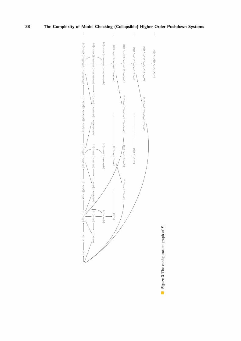
Figure 1 The complexity of model checking order-k higher-order systems. Unless stated, allresults are complete.
logics. In particular, we consider data complexity (formulas are fixed), expression complex-ity (systems are fixed), and combined complexity (both formulas and systems are inputparameters). Table 1 (left column) summarises our results. In all cases, our lower boundshold without the collapse operation, whilst our upper bounds allow collapse.
Basic process algebras (BPAs) are a natural and well-studied subclass of order-1 PDSs (cf.[6]), which are suitable abstractions for modelling the control-flow of sequential programs (cf.[2, 14]). We propose higher-order extensions of BPAs, called (collapsible) higher-order basicprocess algebras (HOBPAs), that form a natural subclass of (collapsible) HOPDSs. Thisdiffers from the single-state HOPDSs introduced by Bouajjani and Meyer [3]. As graphgenerators, (collapsible) HOBPAs are almost as powerful as (collapsible) HOPDSs in thefollowing sense: (1) like CPDS, there exists a collapsible order-2 BPA whose graph has anundecidable monadic second-order logic (MSO) theory, and (2) the class of graphs generatedby order-k BPAs coincide with those generated by order-k PDSs up to MSO interpretations.In this paper, we provide an almost complete picture for the model checking complexities ofstandard temporal logics over (collapsible) HOBPAs. See Table 1 (right column). We showthat the restriction to HOBPA does not, in most cases, simplify the model checking problem;a notable exception is for data complexity, where the problem becomes polynomial time.Again, our lower bounds hold without collapse, whilst our upper bounds allow collapse.
Similar analyses appear across a number of papers for the special case of order-1 push-down systems [1, 6, 30, 31, 4]. In all cases we generalise the resulting picture in a naturalmanner. That is, a 1-ExpTime-complete complexity becomes k-ExpTime-complete, andso on. Our upper bound results concern the data complexity of Collapsible HOBPAs andthe data and combined complexities for LTL over CPDSs. Previous work studied reacha-bility, LTL and the alternation-free µ-calculus [16, 27, 13] over HOPDS without collapse.However, we believe the LTL algorithm contains an error, and provide a new algorithm.Furthermore, the alternation-free µ-calculus algorithm in [16] is not optimal. Our remain-ing results concern lower bounds. We begin with two techniques from in the literature:(1) Engelfriet’s characterization of complexity classes k-ExpTime by extensions of HOPDAs(e.g. with space-bounded worktape) [13], and (2) Cachat and Walukiewicz’s more “direct”approach via encodings of large numbers using HOPDSs [8]. We employ Technique (1) toprove the lower bounds for LTL (and its fragments), CTL, CTL+, and CTL*. This doesnot mean that the proofs of the results are immediate: it was left as an open problem in[8] whether the two techniques can be used to derive these lower bounds. Since Technique(1) seems only suited to deriving k-ExpTime lower bounds (for some k), we give two varia-tions of Technique (2) to derive (k − 1)-ExpSpace lower bounds for EF model checking overHOPDSs and HOBPAs (the latter proof is substantially more involved). The lower boundproofs in this paper suggest that Technique (1) yields simpler proofs, while Technique (2)
M. Hague and A. W. To 3
offers more flexibility.The preliminaries are given in §2. We begin in §3 with the results for fixed formulas over
collapsible HOBPA. In §4 we discuss branching-time logics, and linear-time in §5. Finally,we conclude this paper with future work in §6. Due to the length and intricate nature ofthe proofs, we relegate the full details into the full version.
2 Preliminaries
We define (collapsible) higher-order pushdown systems and basic process algebra and givea result of Engelfriet used in some proofs. Note, after defining higher-order and collapsiblestores, we only define higher-order systems. For the collapsible version, simply replace thehigher-order store with a collapsible one, expanding the stack operations accordingly. Also,the definitions generalise from non-deterministic to alternating in the standard way.
Higher-Order Collapsible Pushdown StoresWe begin by defining a higher-order pushdown store. Collapse links will be introducedafterwards. Intuitively, a higher-order store is a stack of lower order stacks.
I Definition 1 (k-Stores). Let CΣ0 be a finite alphabet Σ with [, ] /∈ Σ. For k ≥ 1, the set of
k-stores CΣk contains all [γ1 . . . γm] with m ≥ 1 and γi ∈ CΣ
k−1 for all 1 ≤ i ≤ m.
There are two operations defined over 1-stores (for all w ∈ Σ∗)
We define pop1 = pushε. Let O1 = pushw | w ∈ Σ∗ . When k > 1, a push operationcreates a copy of the topmost stack, while a pop removes it. We assume w.l.o.g. thatΣ ∩ N = ∅, where N is the set of natural numbers. Finally, let [γ1 . . . γm] ∈ CΣ
k for some k.
pushw[γ1 . . . γm] = [pushw(γ1)γ2 . . . γm]pushl[γ1 . . . γm] = [pushl(γ1)γ2 . . . γm] if 2 ≤ l < k
pushk[γ1 . . . γm] = [γ1γ1γ2 . . . γm]popl[γ1 . . . γm] = [popl(γ1)γ2 . . . γm] if 1 ≤ l < k
popk[γ1 . . . γm] = [γ2 . . . γm] if m > 1topl[γ1 . . . γm] = topl(γ1) if 1 ≤ l < k
topk[γ1 . . . γm] = γ1
Note, when m = 1, popk is undefined. Let Ok = pushw | w ∈ Σ∗ ∪ pushl, popl | 1 <l ≤ k . We designate ⊥ to be a bottom of stack symbol that is neither pushed nor popped.Let [w]1 = [w] and [w]k = [[w]k−1].
For collapse, the order-1 push operation pushw is replaced with pushai11 ...aimm b
for 1 ≤iz ≤ k and az, b ∈ Σ where 1 ≤ z ≤ m. A push
ai11 ...aimm b
on some stack with top1 charactera is equivalent to pusha1...amb except each az is augmented with a pair (iz, 1). That is,the top of stack character a(i,j) is replaced by a(i1,1)
1 . . . a(im,1)m b(i,j). The collapse operation
from a character a(i,j) is equivalent to j applications of popi. The second component j isincremented at every pushi. Hence, (i, j) is a link to the order-(i − 1) stack beneath thecharacter when it was first pushed.
in the copy of a, and, thus, (2, 2) also points to [⊥]. A subtlety occurs after a push3. We
4 The Complexity of Model Checking (Collapsible) Higher-Order Pushdown Systems
obtain the stack below on the left, where the copies of a now refer to the copies of [⊥] withinthe order-2 stack they occupy. After a collapse, we obtain the stack on the right.[ [[
a(2,2) ⊥] [a(2,1) ⊥] [⊥]][[
a(2,2) ⊥] [a(2,1) ⊥] [⊥]] ] [
[[⊥]][[a(2,2) ⊥] [a(2,1) ⊥] [⊥]
] ]Formally, we define order-k stores with links in terms of order-k stores over the infinite
alphabet Σ =a(i,j) | i, j ∈ N
. The set of operations over an order-k store with links is
Ock =push
ai11 ...aimm b
| ∀1 ≤ z ≤ m.1 ≤ iz ≤ k ∧ az ∈ Σ
∪ pushl, popl, collapse | 1 < l ≤ k .
Note that this set of operations is slightly different from the original definition [17]. We show,in the full version, that the definitions are equivalent. The semantics of the operations aregiven below, in terms of the standard order-k pushdown operators, and an order-k stackγ = [γ1 . . . γm]. Let γ<k> be the stack γ where each superscript (i, j) with i ≥ k is replacedwith (i, j + 1).
pushai11 ...aimm b
(γ) = pusha
(i1,1)1 ...a
(im,1)m b
(i′,j′)m
(γ) where top1(γ) = b(i′,j′)
collapse(γ) = popji (γ) where top1(γ) = b(i,j)
pushk[γ1 . . . γm] = [γ<k>1 γ1 . . . γm]pushl[γ1 . . . γm] = [pushl(γ1)γ2 . . . γm] where l < k
Higher-Order Pushdown SystemsA HOPDS is a finite-state system with a higher-order store. The finite-state componentis the control state. At each step, the applicable transitions are determined by the controlstate and the top1 character of the stack. Each transition updates the control state and thestack.
I Definition 2. An order-k PDS is a tuple (P,R,Σ, p0,⊥) where P is a finite set of controlstates, R ⊆ P ×Σ×Ok ×P is a finite set of rules, Σ is a finite stack alphabet, p0 ∈ P is aninitial control state and ⊥∈ Σ is a bottom of stack symbol.
A configuration of a higher-order PDS is a pair 〈p, γ〉 where p ∈ P and γ is a k-store.We have a transition 〈p, γ〉 → 〈p′, γ′〉 iff we have (p, a, o, p′) ∈ R, top1(γ) = a and γ′ = o(γ).The initial configuration is 〈p0, [⊥]k〉.
Higher-Order Basic Process AlgebraAn order-1 BPA is an order-1 PDS with a single control state. By applying the same restric-tion, Bouajjani and Meyer have obtained one definition of higher-order BPA [3]. However,consider 〈p, [[a ⊥]]〉 and the rule (omitting the control) (a, push2). We obtain 〈p, [[a ⊥] [a ⊥]]〉and the same rule can be applied, ad infinitum. However, at order-1 we may use (a, pushbc)to rewrite the top character before adding a new top character. Hence, at order-j, it is natu-ral to be able to rewrite the top order-(j−1) stack, before adding a new one. Consequently,we introduce (a, pushj , b) = pusha; pushj ; pushb for all 2 ≤ j ≤ k. E.g., such rules can sim-ulate push2; push3; pop2. Let O′k = pushw | w ∈ Σ∗ ∪ (a, pushj , b), popj | 1 < j ≤ k .I Definition 3. An order-k BPA is a tuple (R,Σ,⊥) where R ⊆ Σ × O′k is a finite set ofrules, Σ is a finite stack alphabet, and ⊥∈ Σ is the bottom of stack symbol.
M. Hague and A. W. To 5
We mention two results on the expressive power of HOBPAs as graph generators. Famil-iarity with monadic second-order logic (MSO) is assumed (cf. [28]). As graph generators,(collapsible) HOBPAs are as powerful as (collapsible) HOPDAs up to monadic second-orderlogic (MSO) interpretation in the following sense. First, it is known that there exists anorder-2 CPDA generating a graph with an undecidable MSO theory [17]. In contrast, overHOPDAs, MSO is decidable. This CPDA is not a collapsible HOBPA. On the other hand,using the ideas from [17], it is not difficult to come up with an order-2 collapsible HOBPAgenerating a graph with an undecidable MSO theory.
I Proposition 1. There exists a fixed collapsible order-2 BPA which generates a graph withan undecidable MSO theory.
We sketch the proof of this proposition in the full version. Secondly, we discuss the expressivepower of HOBPAs without collapse. Carayol and Wöhrle [9, 10] gave a fixed graph ∆k
2 , foreach integer k > 0, such that the class of graphs that are MSO-interpretable in the graphsgenerated by order-k PDSs coincide with the class of graphs that are MSO-interpretable in∆k
2 . It is easy to check that ∆k2 can be generated by a fixed order-k BPAs (e.g. see [9]),
which implies the following proposition.
I Proposition 2. The class of graphs that are MSO-interpretable in the graphs generated byorder-k BPAs coincide with the class of graphs MSO-interpretable in the graphs generatedby order-k PDSs.
Higher-Order Pushdown Automata with an Auxiliary Work Tape
For the lower bound proofs we use HOPDA with a space-bounded work tape. That is, inaddition to the control state and the stack, the machine has a bounded, two-way work tape.This tape operates identically to the tape in a Turing machine.
I Definition 4. An order-k PDA with an s(n)-space work tape is a tuple (P,R,Σ,Γ ∪ε ,∆, p0,⊥,2,F) where P is a finite set of control states, R ⊆ (P × Γ ∪ ε × Σ ×∆) ×Ok × (∆× l, r × P ) is a finite set of rules, Σ is a finite stack alphabet, Γ is a finite inputalphabet, ∆ is a finite tape alphabet, p0 ∈ P is an initial control state, ⊥∈ Σ is the bottomof stack symbol, 2 ∈ ∆ denotes a blank tape cell and F ⊆ P is a set of accepting controlstates.
Given an input word of length n, a configuration of a HOPDA with s(n) bounded worktape is a tuple 〈p, γ, t, j〉 where p ∈ P , γ is a k-store, t (the tape contents) is a word in ∆s(n)
and 1 ≤ j ≤ s(n) indicates the position of the read/write head on the tape.A rule (p, α, a, x, o, y, d, p′) ∈ R can be applied when the current control state is p, the
input character is α, the top-of-stack character is a, and the tape contents at position j arex. The control state is then updated to p′, the command o is applied to the stack, and y iswritten to the tape. The tape head moves accordingly for d = l (left) or d = r (right).
More formally, we have a transition 〈p, γ, t, j〉 α−→ 〈p′, γ′, t′, j′〉 iff we have
(p, α, a, x, o, y, l, p′) ∈ R, j > 1, top1(γ) = a, t(j) = x, γ′ = o(γ), t′(j) = y, t′(h) = t(h) forall h 6= j and j′ = j−1 or we have (p, α, a, x, o, y, r, p′) ∈ R, j < s(n), top1(γ) = a, t(j) = x,γ′ = o(γ), t′(j) = y, t′(h) = t(h) for all h 6= j and j′ = j − 1. For α 6= ε, we write c α
−→ε c′
whenever there is a sequence of ε-transitions from c to some c1, an α-transition from c1 toc2 and a sequence of ε-transitions to c′. A word α1, . . . , αn is accepted by the automaton iffcn = 〈p, γ〉 and p ∈ F and c0
α1−→ε · · · αn
−→ε cn where c0 = 〈p0, [⊥]k,2s(n), 1〉.
6 The Complexity of Model Checking (Collapsible) Higher-Order Pushdown Systems
Temporal LogicsWe will assume familiarity with the temporal logics discussed, remarking only that µLTL isLTL extended with fixed point operators. Full definitions can be found in the literature [12,29]. We assume, for all logics, the valuations of atomic propositions depend only on thecontrol state and current top-of-stack character, referred to as a head. That is, Λ : P ×Σ→2Prop is an assignment of satisfied atomic propositions from the set Prop to each head inP × Σ. We say a system satisfies a formula if it holds at the initial state of the system.
Engelfriet’s ResultsWe use the following theorem of Engelfriet [13] in some proofs. Let NSPACE(s(n))-P k de-note the class of languages accepted by a non-deterministic order-k PDA with an s(n)-space-bounded work tape, where n is the length of the input word. Similarly, ASPACE(s(n))-P kdenotes the class of languages accepted by an alternating order-k PDA with an s(n)-space-bounded work tape. Finally
⋃d>0 DTIME(expk(ds(n))) is the class of languages accepted
by a time-bounded Turing machine, where exp0(x) = x and expk(x) = 2expk−1(x).
I Theorem 5 ([13], Thm. 2.5). For any k ≥ 1 and s(n) ≥ log(n), we have NSPACE(s(n))-P k = ASPACE(s(n))-P k−1 =
⋃d>0 DTIME(expk(ds(n))).
That is, a non-deterministic order-k PDA with a polynomially-bounded work tape ex-ists for every k-ExpTime language, and an alternating order-k PDA with a polynomially-bounded work tape exists for every (k + 1)-ExpTime language.
3 Model Checking Collapsible HOBPA Against Fixed Formulas
We begin with a P-time algorithm for model checking collapsible HOBPA against fixedformulas. Hardness follows from the P-time-hardness of context-free language emptiness [15].
I Theorem 6. For any logic that can be translated into µ-calculus, model checking collapsibleHOBPA against a fixed formula is in P-time.
Proof. As argued in the full version, any collapsible HOBPA can be simulated by a CPDSwith a fixed number of control states. Therefrom, and since the formula is fixed, we constructa CPDS parity game with a fixed number of control states. At order-k, the winner of thesegames can be determined in k-ExpTime in the number of control states, and polynomial inthe alphabet [17]. Hence, the algorithm runs in P-time. J
4 Branching Time
We begin by observing, for CPDS, the upper bounds for CTL, CTL+ and CTL* can beobtained by translating into µ-calculus, which has a k-ExpTime model checking problem.For CTL, the translation is polynomial. For CTL+ and CTL* it is exponential, giving(k + 1)-ExpTime, and k-ExpTime when the formula is fixed. For the lower bound results,we discuss EF, CTL and then CTL+.
I Theorem 7. For a fixed formula, and a given order-k CPDS, model checking CTL, CTL+and CTL* is in k-ExpTime. For a non-fixed system and non-fixed formula, CTL is k-ExpTime, and CTL+ and CTL* are in (k + 1)-ExpTime.
M. Hague and A. W. To 7
4.1 Lower Bounds for EFIn most cases, we are able to derive optimal lower bounds using Theorem 5. However,Theorem 5 is not immediately applicable for (e.g.) (k − 1)-ExpSpace problems. In thecase of EF-logic, the model checking problem over order-1 PDSs and BPAs is PSpace-complete [25, 31]. We now give (k − 1)-ExpSpace lower bounds for data complexity oforder-k PDSs and the expression complexity of order-k BPAs (and thus of order-k PDSs)using the technique of [8] of encoding large numbers. We conjecture that these lower boundsare tight (currently, the best upper bound is k-ExpTime, which is inherited from µ-calculus).
I Theorem 8. Model checking EF over order-k PDS without collapse is (k − 1)-ExpSpace-hard, even for a fixed formula.
Proof. (sketch) We reduce membership for a given (k − 1)-ExpSpace Turing machine Musing expk−1(p(n)) space on an input word of length n, for some polynomial function p. Fixa number m ∈ Z>0, which we will later define as p(n) once n is set. The proof combines thetechnique of [1] for proving that EF-logic over PDS is PSpace-hard and the technique of [8]for encoding and checking large numbers (i.e. k-towers of exponentials) using operations inOk.
We shall start by briefly recalling the encoding techniques of large numbers from [8]. Foreach i ∈ Z>0, we define Σi := ai, bi and Σ≤i :=
⋃ij=1 Σi. We now define the notion of
i-counters by induction. A 1-counter (of length m) is a word σm−1 . . . σ0 ∈ (Σ1)m. Such aword naturally represents the number
∑m−1i=0 σi2i where a1 represents 0 and b1 represents
1. Assuming that the notion of i-counter has been defined, an (i + 1)-counter is simply aword σrlr . . . σ0l0 over Σ≤i+1, where r = expi(m) − 1, σj ∈ Σi+1, and lj is an i-counterrepresenting the number j. This (i + 1)-counter represents the number
∑rj=0 σj2j , where
(as before) ai+1 and bi+1 are used to (respectively) represent 0 and 1.Cachat and Walukiewicz [8] showed that a polynomial-size order-k pushdown game arena
P with a reachability objective could be defined (depending only on m) with the followingcontrol states and properties: counterk — from configuration (counterk, γ) of P, Player0 wins iff γ ends with a k-counter; firstk (resp. lastk) — from configuration (firstk, γ)(resp. (lastk, γ), Player 0 wins iff γ ends with a k-counter representing 0 (resp. expk−1(m));equalk — from (equalk, γ), Player 0 wins iff γ ends with two k-counters representing equalvalues; succk — from (succk, γ), Player 0 wins iff γ ends with two k-counters representingsuccessive values. We observe that the game element of P can easily be translated into fixedEF formulas (i.e. not depending onm) satisfying the same properties, the main reason beingthat the game arena P has a fixed number of rounds.
The rest of the proof uses the idea of [1]. Using an EF operator, we will first guessa word in Σ≤k+1 representing an accepting computation of M on the given input wordw = α1 . . . αn. We then need to check that the guess is valid. That is, it represents asequence of configurations, the initial configuration is the right form, the final configurationis reached, and consecutive configurations respect the transition relation. All these can bedone by means of a fixed formula, thanks to the result above for encoding large numbers. J
I Theorem 9. For a fixed order-k HOBPA without collapse, model checking EF is (k − 1)-ExpSpace-hard.
Proof. (sketch) The proof uses some general ideas from the previous proof, but, withoutcontrol states to encode tests for large numbers, we need an entirely different construction.We briefly explain the order-2 case. Our HOBPA P will guess an accepting run of a fixedexponential space Turing machineM accepting an ExpSpace-complete language, obtaining a
8 The Complexity of Model Checking (Collapsible) Higher-Order Pushdown Systems
stack of the form [w]2. For the checking stage, our HOBPA P now tries to find some locationinside the stack that is invalid. In doing so, we need to ensure that all of the informationon top of this location is not destroyed. To this end, we will build a stair-like structurefrom [w]2 by performing operations of the form [push1(a′); push2; push1(prime)] or of theform [push1(a′′); push2; push1(dprime)] when seeing a topmost stack symbol a. Here, primeand dprime are simply intermediate symbols to help signify the action that was previousexecuted, i.e., we could simply only allow pop1 operation when prime or dprime is seen astopmost symbol. The double prime marking is used to “remember” the starting point of(sub)configuration that we suspect is invalid. That is, we will have to make sure that it isput precisely once. At some point, P simply applies rules of the form push1(a′) when a isseen without applying push2, which marks the end point of a (sub)configuration that wesuspect is invalid. We then only allow rules pop2 when primed or double primed symbolsare seen. To make sure that we see precisely one separator symbol (i.e. a3 ∈ Σ3), we canuse an EF formula saying facts about the location of the double primed symbol a′′3 . Such astair-like structure will allow us to define EF formulas that play the roles of counteri, firsti,lasti, equali, and succi and their associated EF formulas in the previous proof. J
4.2 Lower Bounds for CTLData Complexity We know, for a fixed formula, model checking CTL, CTL+ and CTL*against HOPDSs is in k-ExpTime. Here, we show the lower bound.
I Theorem 10. For a fixed formula, model checking CTL over a given order-k HOPDSwithout collapse is k-ExpTime-hard.
Proof. (sketch) From Theorem 5 we take a language that is k-ExpTime-hard and fix anequivalent order-(k− 1) alternating HOPDA with a polynomially space-bounded work tapeP. The reduction is inspired by Bozzelli [4].
We use an order-k stack to navigate a computation tree of the HOPDA. To simulate thework tape, at each step, after an operation on the order-(k − 1) stack, a sequence of tapesymbols are pushed on to the top order-1 stack. Then, the system can do a check branch toensure the guessed tape is consistent with the previous, or continue simulating the execution.To continue, an order-k push saves the current state (for backtracking), the work tape iserased, the next rule is announced, and a pushk remembers the rule. This process repeats.Consider the example order-3 stack below. [tw1]
[w2]. . .
[[r . . .]. . .
] [t′w′1][w′2]. . .
· · ·
This stack is at a configuration with the tape given by the word t and order-2 stack[[w1] [w2] . . .], which can backtrack to a configuration with tape t′ and order-2 stack[[w′1] [w′2] . . .]. The rule r connects the configurations. When an accepting configurationis seen, or the children of the current node have been fully explored, we backtrack usingpopk, and check untested universal branches. The automaton accepts when the (marked)initial stack is reached. That is, all paths have been explored, and found to be accepting.
The check branches have further branches for each of the polynomially many positionsof the work tape. Each branch uses the control state to find the correct position, and then,using the control state, compares it with the corresponding positions in the previous worktape, which is recovered via popk operations.
M. Hague and A. W. To 9
The CTL formula E ((op ∧AX(check → AFgood))Ufin) asserts a path encoding anaccepting tree exists, and checking branches all accept. The proposition op indicates thecurrent path is simulating a tree, and check indicates a checking branch. Finally, goodindicates that the check has been passed, and fin denotes the (successful) completion of therun. J
Expression Complexity The following theorem takes care of all cases.
I Theorem 11. For a fixed order-k HOBPA without collapse, model checking CTL is k-ExpTime-hard.
Proof. (sketch) The proof is in stages. First, we adapt Theorem 10, unfixing the formula tofix the HOPDS. A HOBPA is obtained using a more complex formula. There are two mainassertions we move from the HOPDS to the formula. First, the check branch becomes astraight-line sequence of pops and the formula uses sequences of EX to compare positions.Secondly, the word position being read has to be guessed and added to the work tapeinformation, then checked by the formula. Hence, we have the result for a fixed HOPDS.
To obtain a HOBPA the main difficulty is that control states were used to separate thecheck, backtrack and simulation phases of the model. Here we use the (a, pushj , b) rulesso that, when pushing, the automaton can read a character a, and mark it a in the nextapplied rule. Hence the system knows when it is moving up or down the stack, and whenit has simulated a stack action. Also the automaton announces the intended phases. Forexample, the check branch announces “check”, removes the work tape, announces “popk”,pops, announces “check” again and removes the work tape. The formula can then use EXj
to look into the first tape, and E(tapeU(popk ∧ EX(check ∧ EXjϕ))) to look j steps intothe next tape, where tape indicates that a tape character is seen. J
4.3 Lower Bounds for CTL+
For data complexity, the CTL lower bound transfers to CTL+ and CTL*. For the expressioncomplexity, the following theorem suffices.
I Theorem 12. For a fixed order-k HOBPA without collapse, model checking CTL+ is(k + 1)-ExpTime-hard.
Proof. (sketch) First we adapt the proof of Theorem 10 to show, CTL* is (k + 1)-ExpTime-hard. We then replace the CTL* formula with a CTL+ formula. Then we show how to fixthe system, and restrict ourselves to HOBPA.
For a non-fixed formula and system, our CTL* proof adapts Bozzelli’s order-1 proof [4].Fix a language that is hard for (k + 1)-ExpTime and an equivalent order-(k−1) alternatingHOPDA with an exponentially space-bounded work tape. The system proceeds as before,but guesses the length of the work tape and uses a word binn(0)c0binn(1)c1 · · · binn(2n −1)c2n−1 to represent it, where binn(i) is the n-digit binary representation of i, and cj are cellcontents. The check phase has one branch to check the cell counters are sequential, and theothers, instead of just popping down the stack, mark a position in each tape. The formulaasserts, when markings are sensible, the tape contents are locally consistent. This can, infact, be encoded in CTL+ by taking advantage of straight-line parts of the execution andadding extra markings. Obtaining a fixed HOBPA is similar to the CTL case, with someextra tricks. E.g., to ensure each marker is placed once and in the correct order. J
10 The Complexity of Model Checking (Collapsible) Higher-Order Pushdown Systems
5 Linear Time
We consider the linear time logics. We first deal with the upper bound for linear timeµ-calculus (µLTL) — and hence LTL — before considering the lower bounds in turn.
5.1 Upper Bounds for µLTLSince the linear time µ-calculus (µLTL) does not translate polynomially into µ-calculus, weshow the k-ExpTime upper bound of model checking µLTL against CPDS separately. Notethat µLTL trivially subsumes all other linear time logics considered in this paper.
I Theorem 13. Model checking µLTL against order-k CPDSs is in k-ExpTime for a non-fixed formula, and (k − 1)-ExpTime for a fixed formula.
Proof. (sketch) We can translate any µLTL formula ϕ into a Büchi automaton B at anexponential cost [29]. From a given CPDS P we construct a product CPDS PB = P × Bwhich has a Büchi acceptance condition such that PB accepts iff P does not satisfy ϕ.
An order-k Büchi CPDS is a CPDS parity game with two colours and only one player.Hence, non-emptiness can be reduced to determining the winner in a parity game, whichtakes k-ExpTime in the size of the CPDS [17]. Since the Büchi CPDS is exponential inthe size of ϕ, this complexity is too high. The algorithm for an order-k parity game is bya reduction to an order-(k − 1) game of exponential size. Because the Büchi CPDS hasone player, we can avoid the exponential blow up, constructing an order-(k − 1) game ofpolynomial size. This can be solved in (k − 1)-ExpTime in the size of the Büchi CPDS,giving an algorithm in k-ExpTime for a non-fixed formula, and (k − 1)-ExpTime for a fixedformula. J
5.2 Lower Bounds for LTLWe first give a matching lower bound for data complexity (fixed formula) of LTL, whichalready hold for its fragments LTL(F,X) and LTL(U). Since we have previously shown thatorder-k HOBPA can be analysed in P-time for fixed formulas, it remains to consider HOPDS.
I Theorem 14. Model checking HOPDS without collapse against fixed LTL(F, X) andLTL(U) formulas is (k − 1)-ExpTime-hard.
Proof. The non-emptiness problem for HOPDS is (k − 1)-ExpTime-complete [13]. Thisproblem easily reduces to checking the fixed formula G(¬f), where f holds at all acceptingstates. Since this formula is both in LTL(F, X) and LTL(U), we are done. J
Next we study the expression complexity (fixed system). This is our main result of thissection: already for a fixed order-k HOBPA, both LTL(F, X) and LTL(U) are k-ExpTime-hard.
I Theorem 15. Model checking LTL(F, X) and LTL(U) against a fixed HOBPA withoutcollapse is k-ExpTime-hard.
Proof. (sketch) We take a k-ExpTime-hard language L, and, by Theorem 5, its equivalentHOPDS with s(n)-bounded space work tape P, for some polynomial s(n). We shall constructa fixed HOBPA P ′ such that the language L is polynomial-time reducible to the LTL(F,X)model checking problem over P ′. We can similarly derive the desired lower bound for LTL(U)by “weakly” simulating the next operators with the until operator in the standard way.
M. Hague and A. W. To 11
We shall now give an intuition of the construction of P ′. Our HOBPA P ′ is an “over-approximation” of P in the sense that P ′ can do whatever actions P can do but also more.We will then use LTL(F,X) formulas to enforce correct simulations. This is of course dueto the fact that P ′ lacks control states and work tape, and its definition should not dependon the input word to P. We shall now elaborate more on how this can be implemented.Given a word w = α1 . . . αn ∈ Γ∗, we would like to determine if there is an accepting runof P on w, i.e., a sequence of configurations of the form 〈p, γ, t, j〉 starting with a startingconfiguration and ending with a final configuration. Here, p is a control state of P, γ is ak-store, t ∈ ∆s(n) is a tape content, and 1 ≤ j ≤ s(n) is the position of the tape head. Wewill represent each such configuration as the topmost symbols of a contiguous sequence ofconfigurations of P ′. For example, suppose that the current configuration of P is 〈p, γ, t, j〉where top1(γ) = a. The HOBPA P ′ will start by having (p, a) as its topmost stack symbol.It will then keep modifing its topmost symbol to reflect the tape content t and the position j.This is done by guessing each individual tape cell content from left to right. At some point,P ′ will nondetermistically choose some rule of P to fire. We simulate this by first executingthe stack operation and then guess some new state, which we put on top of the stack (thisguess is needed because pop operations will destroy control state information). It will thencontinue by guessing next tape content in the same manner. This process can be repeatedindefinitely, unless P ′ decides to go to a final (i.e. sink) state, in which P ′ will just loopforever. Given an input word w = α1 . . . αn ∈ Γ∗, we may force a correct simulation of P onw by P ′ using an LTL(F,X) formula. That is, we give a formula ϕw such that w ∈ L(P) iffP ′, c0 6|= ϕw, where c0 is an appropriate initial configuration of P ′ reflecting the initial stateof P. This can be done by first ensuring that each configuration of P in the simulation as acontiguous sequence of configurations of P ′ is valid. In particular, the guessed tape content(reflected by the topmost symbols in this sequence of configurations of P ′) must be of lengths(n) and has precisely one tape head, which can be easily expressed in LTL(F,X) using asingle operator G and nestings of next operators of depth s(n) (approximately). Recall thats(n) is a polynomial function. Using the same technique, we also express that two represen-tations of consecutive configurations of P in the simulation respect the transition relationof P. Similarly, we enforce the initial configuration in the simulation and that some finalconfiguration of P is reached. J
6 Future Work
There are several avenues of future work. E.g., we have no matching upper bound forthe complexity of EF model checking. Walukiewicz has shown the problem to be PSpace-complete at order-1 [31]. However, his techniques do not easily extend to HOPDS owing tothe subtleties of higher-order stacks. We may also study simpler logics such as LTL(F).Acknowledgments. We thank Olivier Serre for interesting discussions and the anonymousreferees for their helpful remarks. This work was partly supported by EPSRC (EP/F036361and EP/E005039), and was done while the second author was a student at the School ofInformatics, University of Edinburgh.
References1 A. Bouajjani, J. Esparza, and O. Maler. Reachability analysis of pushdown automata: Ap-
plication to model-checking. In CONCUR, p. 135–150, 1997.2 A. Bouajjani, P. Habermehl, and R. Mayr. Automatic verification of recursive procedures
with one integer parameter. Theor. Comput. Sci. 295:85–106 (2003)
12 The Complexity of Model Checking (Collapsible) Higher-Order Pushdown Systems
3 A. Bouajjani and A. Meyer. Symbolic Reachability Analysis of Higher-Order Context-FreeProcesses. In FSTTCS, p. 135–147, 2004.
4 L. Bozzelli. Complexity results on branching-time pushdown model checking. Theor. Comput.Sci., 379(1-2):286–297, 2007.
5 C. Broadbent and L. Ong. On global model checking trees generated by higher-order recursionschemes. In FOSSACS, p. 107–121, 2009.
6 O. Burkart, D. Caucal, F. Moller, and B. Steffen. Verification on infinite structures. InHandbook of Process Algebra, Elsevier, 1999.
7 T. Cachat. Higher order pushdown automata, the caucal hierarchy of graphs and paritygames. In ICALP, p. 556–569, 2003.
8 T. Cachat and I. Walukiewicz. The complexity of games on higher order pushdown automata.CoRR, abs/0705.0262, 2007.
9 A. Carayol. Regular sets of higher-order pushdown stacks. In MFCS, p. 168–179, 2005.10 A. Carayol and S. Wöhrle. The caucal hierarchy of infinite graphs in terms of logic and
higher-order pushdown automata. In FSTTCS, p. 112–123, 2003.11 D. Caucal. On infinite terms having a decidable monadic theory. In Proc. MFCS, p. 165–176,
2002.12 E. A. Emerson. Temporal and modal logic. In Handbook of Theoretical Computer Science, p.
995–1072, Elsevier, 1990.13 J. Engelfriet. Iterated pushdown automata and complexity classes. In STOC, p. 365–373,
1983.14 J. Esparza and J. Knoop. An automata-theoretic approach to interprocedural data-flow
analysis. In FoSSaCS, p. 14–30, 1999.15 E. M. Gurari. An Introduction to the Theory of Computation. W. H. Freeman & Co., New
York, NY, USA, 1989.16 M. Hague. Global Model Checking Higher Order Pushdown Systems. PhD thesis, Oxford
University, 2009.17 M. Hague, A. S. Murawski, C.-H. L. Ong, and O. Serre. Collapsible pushdown automata and
recursion schemes. In LICS, p. 452–461, 2008.18 T. Knapik, D. Niwinski, and P. Urzyczyn. Higher-order pushdown trees are easy. In FoSSaCS,
p. 205–222, 2002.19 T. Knapik, D. Niwinski, P. Urzyczyn, I. Walukiewicz. Unsafe Grammars and Panic Automata.
In ICALP, p. 1450-1461, 2005.20 N. Kobayashi. Model-checking higher-order functions. In PPDP, p. 25–36, 2009.21 N. Kobayashi. Types and higher-order recursion schemes for verification of higher-order
programs. In POPL, p. 416–428, 2009.22 N. Kobayashi and C.-H. L. Ong. Complexity of model checking recursion schemes for frag-
ments of the modal mu-calculus. In ICALP, p. 223–234, 2009.23 N. Kobayashi and C.-H. L. Ong. A type system equivalent to the modal mu-calculus model
checking of higher-order recursion schemes. In LICS, p. 179–188, 2009.24 A. N. Maslov. Multilevel stack automata. Probl. Inf. Transm., 15:1170–1174, 1976.25 R. Mayr. Strict lower bounds for model checking BPA. Electr. Notes Theor. Comput. Sci.,
18, 1998.26 C.-H. L. Ong. On model-checking trees generated by higher-order recursion schemes. In LICS,
p. 81–90, 2006.27 A. Seth. An Alternative Construction in Symbolic Reachability Analysis of Second Order
Pushdown Systems. Int. J. Found. Comput. Sci. 19(4): 983-998, 2008.28 W. Thomas. Constructing Infinite Graphs with a Decidable MSO-Theory. In MFCS, p.
113–124, 2003.29 M. Vardi. A temporal fixpoint calculus. In POPL, p. 250-259, 1988.30 I. Walukiewicz. Pushdown processes: Games and model checking. In CAV, p. 62–74, 1996.31 I. Walukiewicz. Model checking CTL properties of pushdown systems. In FSTTCS, p. 127–
138, 2000.
M. Hague and A. W. To 13
A Definition of Collapsible Pushdown Systems
We define order-k stores with links in terms of order-k stores over the infinite alphabetΣ =
a(i,j) | i, j ∈ N
. We define the original set of stack operations [17]. We then define
the rule pushai11 ...aimm b
used in this paper.The set of operations over an order-k store with links is
Ock =pushia, rewa, pop1 | 1 ≤ i ≤ k ∧ a ∈ Σ
∪ pushl, popl, collapse | 1 < l ≤ k .
The semantics of the operations are given below, in terms of the standard order-k pushdownoperators, and an order-k stack γ = [γ1 . . . γm]. Let γ<k> be the stack γ where eachsuperscript (i, j) with i ≥ k is replaced with (i, j + 1).
pop1(γ) = pushε(γ)rewa = pusha(i,j) where top1(γ) = b(i,j)
pushia(γ) = pusha(i,1)b
(i′,j′)m
(γ) where top1(γ) = b(i′,j′)
collapse(γ) = popji (γ) where top1(γ) = b(i,j)
pushk[γ1 . . . γm] = [γ<k>1 γ1 . . . γm]pushl[γ1 . . . γm] = [pushl(γ1)γ2 . . . γm] where l < k
I Definition 16. An order-k CPDS is a tuple (P,R,Σ, p0,⊥) where P is a finite set ofcontrol states, R ⊆ P × Σ × Ock × P is a finite set of rules, Σ is a finite stack alphabet,p0 ∈ P is an initial control state and ⊥∈ Σ is a bottom of stack symbol.
A configuration of a CPDS is a pair 〈p, γ〉 where p ∈ P and γ is a k-store with links. Wehave a transition 〈p, γ〉 → 〈p′, γ′〉 iff we have (p, a, o, p′) ∈ R, top1(γ) is a or a(i,j) for somei, j and γ′ = o(γ). The initial configuration is 〈p0, [⊥]k〉.
In this paper we use a slight variation of CPDSs, where
Ock =push
ai11 ...aimm b
| ∀1 ≤ z ≤ m.1 ≤ iz ≤ k ∧ az ∈ Σ
∪ pushl, popl, collapse | 1 < l ≤ k .This is to emphasize the connection to HOPDS. We have
pushai11 ...aimm b
= rewb; pushimam ; . . . ; pushi1a1
This can easily be simulated by adding (a polynomial number of) intermediate states.Finally, we observe that a collapsible HOBPA can be simulated by a CPDS of the original
definition with a fixed number of states and a polynomially expanded alphabet. To do sowe expand the alphabet to two kinds of tuples
HOPush(a, j, b) and CPush(a, ai11 , . . . , aimm )
for all prefixes ai11 , . . . , aimm of some collapsible push rule. For both tuples, a is the top1character of the stack being simulated. We write 〈a〉 to denote any character of this form,or simply of the form a.
The first tuple HOPush(a, j, b) indicates the current top1 character is a, a pushjis to be performed, then the top1 character is to be replaced by b. We replaceeach rule (a, (b, pushj , c)) with the rules (qnorm, 〈a〉, pushHOPush(b,j,c), qpush) for all j′ ∈1, . . . , k and a ∈ Σ, followed by the rule (qpush, HOPush(b, j, c), pushj , qpushed) and(qpushed, HOPush(b, j, c), pushc, qnorm).
14 The Complexity of Model Checking (Collapsible) Higher-Order Pushdown Systems
The second type of tuples CPush(a, ai11 , . . . , aimm ) are used to simulate collapsible pushrules. That is, we still need to perform pushi1a1
; . . . ; pushimam . Each rule (a, pushai11 ...aimm b
) isreplaced by (qnorm, 〈a〉, rewCPush(b,ai11 ,...,aimm ),qcpush . Then we add the rule
whenever m > 0 for all prefixes of collapsible push rules. Finally we have the rule
(qcpush, CPush(b), rew(b), qnorm) .
The remaining rules (a, o) are simply replaced by rules of the form (qnorm, 〈a〉, o, qnorm).
B Proofs for Branching Time
B.1 Proof of Theorem 8
Theorem 8. Model checking EF over order-k PDS without collapse is (k − 1)-ExpSpace-hard, even for a fixed formula.
We will now elaborate our construction of the fixed EF formulas and the order-k PDSsin more details. Following [8], we could construct in polynomial-time an order-k PDS Pover the stack alphabet Σ≤k+1 with the following pairs (s, ψ) of control states of P and EFformulas:
(counterk, Counterk) such that (P, 〈counterk, γ〉) |= Counterk iff top2(γ) ends with ak-counter.(firstk, F irstk) such that (P, 〈firstk, γ〉) |= Firstk iff top2(γ) ends with a k-counterrepresenting the number 0.(lastk, Lastk) such that (P, 〈lastk, γ〉) |= Lastk iff top2(γ) ends with a k-counter repre-senting the number expk−1(m)− 1.(equalk, Equalk) such that (P, 〈equalk, γ〉) |= Equalk iff top2(γ) ends with two k-countersthat have the same value (separated by one letter from Γk+1).(equal2k, Equal2k) such that (P, 〈equal2k, γ〉) |= Equal2k iff the two topmost order-1 stacksin γ ends with k-counters that have the same value.(succk, Succk) such that (P, 〈succk, γ〉) |= Succk iff top2(γ) ends with two k-countersthat are of successive values (the top one is the successor of the lower one).
The EF formulas defined here depend neither on the input word w nor on the Turing machineM . In fact, [8] defines order-k pushdown game arenas instead of EF formulas. However, onecan easily check that the description translates directly to pairs of EF formulas and HOPDSas they have a fixed number of rounds (more precisely, the structure of the arena is a treewith no self-loops).
We now describe how to finish the proof. Suppose that M uses expk−1(p(n)) space andt states. Set m = (log2(t) + 1) × p(n). A configuration of M can be thought of as a wordfrom 0, 1∗ of length (log2(t) + 1)× (expk−1(p(n))− 1), where each tape cell of M is nowrepresented using log(t) + 1 bits as: (1) we need one bit to tell whether head is on topof the current cell, (2) we need one bit to store whether the current tape cell has 0 or 1(wlog we can assume that the tape alphabet of M is 0, 1), and (3) assuming that thehead is on top of the current tape cell, we need log2(t) − 1 bits to describe which state Mis in. In this way, we can represent a configuration of M as a k-counter. Note that the ithcell in a configuration of M corresponds to the contiguous sequence of bits in the number
M. Hague and A. W. To 15
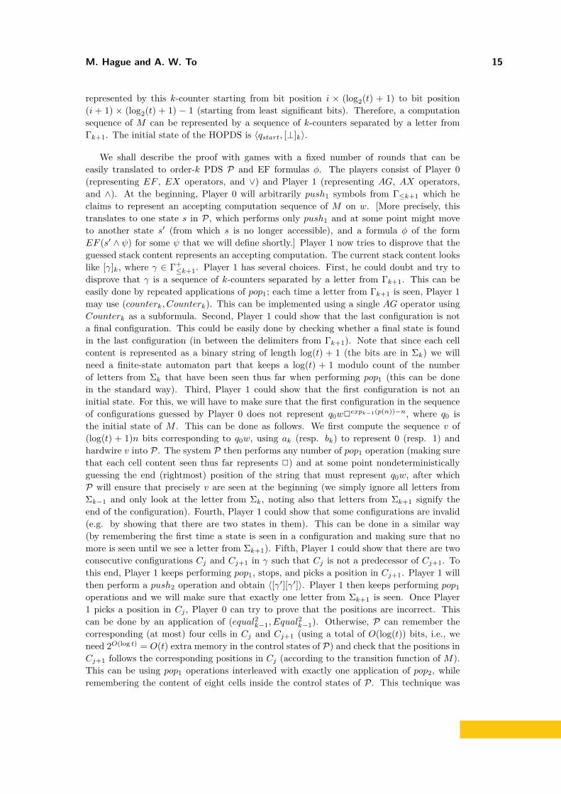
represented by this k-counter starting from bit position i × (log2(t) + 1) to bit position(i + 1) × (log2(t) + 1) − 1 (starting from least significant bits). Therefore, a computationsequence of M can be represented by a sequence of k-counters separated by a letter fromΓk+1. The initial state of the HOPDS is 〈qstart, [⊥]k〉.
We shall describe the proof with games with a fixed number of rounds that can beeasily translated to order-k PDS P and EF formulas φ. The players consist of Player 0(representing EF , EX operators, and ∨) and Player 1 (representing AG, AX operators,and ∧). At the beginning, Player 0 will arbitrarily push1 symbols from Γ≤k+1 which heclaims to represent an accepting computation sequence of M on w. [More precisely, thistranslates to one state s in P, which performs only push1 and at some point might moveto another state s′ (from which s is no longer accessible), and a formula φ of the formEF (s′ ∧ ψ) for some ψ that we will define shortly.] Player 1 now tries to disprove that theguessed stack content represents an accepting computation. The current stack content lookslike [γ]k, where γ ∈ Γ+
≤k+1. Player 1 has several choices. First, he could doubt and try todisprove that γ is a sequence of k-counters separated by a letter from Γk+1. This can beeasily done by repeated applications of pop1; each time a letter from Γk+1 is seen, Player 1may use (counterk, Counterk). This can be implemented using a single AG operator usingCounterk as a subformula. Second, Player 1 could show that the last configuration is nota final configuration. This could be easily done by checking whether a final state is foundin the last configuration (in between the delimiters from Γk+1). Note that since each cellcontent is represented as a binary string of length log(t) + 1 (the bits are in Σk) we willneed a finite-state automaton part that keeps a log(t) + 1 modulo count of the numberof letters from Σk that have been seen thus far when performing pop1 (this can be donein the standard way). Third, Player 1 could show that the first configuration is not aninitial state. For this, we will have to make sure that the first configuration in the sequenceof configurations guessed by Player 0 does not represent q0w2expk−1(p(n))−n, where q0 isthe initial state of M . This can be done as follows. We first compute the sequence v of(log(t) + 1)n bits corresponding to q0w, using ak (resp. bk) to represent 0 (resp. 1) andhardwire v into P. The system P then performs any number of pop1 operation (making surethat each cell content seen thus far represents 2) and at some point nondeterministicallyguessing the end (rightmost) position of the string that must represent q0w, after whichP will ensure that precisely v are seen at the beginning (we simply ignore all letters fromΣk−1 and only look at the letter from Σk, noting also that letters from Σk+1 signify theend of the configuration). Fourth, Player 1 could show that some configurations are invalid(e.g. by showing that there are two states in them). This can be done in a similar way(by remembering the first time a state is seen in a configuration and making sure that nomore is seen until we see a letter from Σk+1). Fifth, Player 1 could show that there are twoconsecutive configurations Cj and Cj+1 in γ such that Cj is not a predecessor of Cj+1. Tothis end, Player 1 keeps performing pop1, stops, and picks a position in Cj+1. Player 1 willthen perform a push2 operation and obtain 〈[γ′][γ′]〉. Player 1 then keeps performing pop1operations and we will make sure that exactly one letter from Σk+1 is seen. Once Player1 picks a position in Cj , Player 0 can try to prove that the positions are incorrect. Thiscan be done by an application of (equal2k−1, Equal
2k−1). Otherwise, P can remember the
corresponding (at most) four cells in Cj and Cj+1 (using a total of O(log(t)) bits, i.e., weneed 2O(log t) = O(t) extra memory in the control states of P) and check that the positions inCj+1 follows the corresponding positions in Cj (according to the transition function of M).This can be using pop1 operations interleaved with exactly one application of pop2, whileremembering the content of eight cells inside the control states of P. This technique was
16 The Complexity of Model Checking (Collapsible) Higher-Order Pushdown Systems
first used in [1] to encode linear bounded Turing machine as an EF model checking problem(for a fixed formula) over order-1 PDSs. Finally, we can see that the resulting EF-formulais fixed and the size of the resulting HOPDS is polynomial in |w| and |M | (recall also thatM is fixed). This completes the proof.
B.2 Proof of Theorem 9
Theorem 9. For a fixed order-k HOBPA without collapse, model checking EF is (k − 1)-ExpSpace-hard.
We use the notion of i-counters from the previous proof. Fix positive integers n andk > 1. Fix a polynomial function p. For a finite set Q, a (k,Q)-counter is a word of theform σrlr . . . σ0l0 where
each σi is a letter in Σk ∪Q,each li is a (k − 1)-counter representing the number i, andr = expk(p(n))− 1.
Note that the notions of k-counters and (k, ∅)-counters coincide. We shall now define an order2-BPA P := P2,Q = (R,Σ, c0) that depends only on Q and show that EF model checkingover P is 1-ExpSpace-hard. We will later set Q to be the set of states of a fixed (k − 1)-ExpSpace-complete Turing machine. We will then argue that the same construction canbe generalised to show (k − 1)-ExpSpace-hard expression complexity of EF model checkingover k-BPAs.
At the beginning, our 2-BPA must write a sequence of (2, Q)-counters that potentiallygives an accepting computation of a fixed 1-ExpSpace-complete Turing machine. Sincethe definition should not depend on the input word of a fixed Turing machine, we definethe languages L2 := (Σ+
1 (Σ2 ∪ Q))+ and L′2 := (L2Σ3)+. Intuitively, L2 is the smallest“overapproximation” of the notion of (2, Q)-counters that does not depend on n. Hence,L′2 is an overapproximation of all sequences of (2, Q)-counters separated by a letter fromΣ3. Initially our 2-BPA will be able to guess a word in L′2, i.e., a potential sequence of(2, Q)-counters separated by a letter in Σ3. The starting configuration c0 is [(guess, 3)]kwhere (guess, 3) is a symbol in Σ. We add the following rules to R:
((guess, 3), push((guess, 2)σ3)) for each σ3 ∈ Σ3,((guess, 2), push((guess, 1)σ2)) for each σ2 ∈ Σ2 ∪Q,((guess, 1), push((guess, 1)σ1)) for each σ1 ∈ Σ1,((guess, 1), push((guess, 2′)σ1)) for each σ1 ∈ Σ1,((guess, 2′), push((guess, 3)), and((guess, 2′), pop1) for each σ3 ∈ Σ3.
The last transition marks the end of the guessing stage as we will no longer see stack symbolof the form (guess, i) afterwards. We now introduce several transitions that will allow us touse EF formulas to check the correctness of the guess from the previous stage. For i = 1, 2, 3,let Σ′i := a′i, b′i and Σ′′i := a′′i , b′′i . Also, let Q′ = q′ : q ∈ Q and Q′′ = q′′ : q ∈ Q.Let Prime := Q′ ∪⋃3
i=1 Σ′i and DPrime := Q′′ ∪⋃3i=1 Σ′′i . Add the following rules:
For i = 1, 2, 3, when σi ∈ Σi is seen, we can nondeterministically choose any of thefollowing four choices:push1(σ′i)push1(σ′′i )(σ′i, push2, unmarkedi)(σ′′i , push2,markedi)
When q ∈ Q is seen, we can nondeterministically choose any of the following four choices:
For i = 1, 2, 3, when we see either σ′i ∈ Σ′i ∪ Q′ or σ′′i ∈ Σ′′i ∪ Q′′, we can only performpop2.For i = 1, 2, 3, when we see either markedi, unmarkedi, markedQ, or unmarkedQ, wecan only perform pop1.
To get an intuition, let us look at an example. Suppose that the current stack content is[a3b1a1qb1b1a3]2. The following is a snapshot of a run:
In this way, we obtain a stair-like structure from the stack content [w]2 from the initialguessing stage. That is, we “unroll” the content of the topmost 1-store.The following aresimple properties that can be established about every reachable configuration c of P2,Q:(P1) Every 1-store in c has at most one symbol from (Q′ ∪ Q′′) ∪ ⋃3
i=1(Σ′i ∪ Σ′′i ), i.e., onthe top of the store.
(P2) If c |= (Q′ ∪Q′′) ∪⋃3i=1(Σ′i ∪ Σ′′i ) and c →∗ c′, then c′ |= (Q′ ∪Q′′) ∪⋃3
i=1(Σ′i ∪ Σ′′i )too.
We now will define several EF formulas that play the roles of Counteri, Equali, etc. inthe previous proof. These formulas shall depend on the parameter n and the polynomialp. First, we can easily define Counterp(n)
1 such that P2,Q, c |= Counterp(n)1 iff the topmost
p(n) + 2 symbols on the topmost 1-store of c is of the form σ2vγ2 for some σ2, γ2 ∈ Σ2 ∪Qand some v ∈ (Σ1)p(n). This can be done using nested EX operators, conjunctions, atomicpropositions, and no EF operators, since we have to unroll the topmost 1-store up to p(n)+2times. Similarly, we can define Firstp(n)
1 (resp. Lastp(n)1 ) such that P2,Q |= First
p(n)1 (resp.
P2,Q |= Lastp(n)1 ) iff the topmost p(n) + 2 symbols on the topmost 1-store of c is σ2vσ
′2 for
σ2, σ′2 ∈ Σ2 ∪Q and v = a
p(n)1 (resp. v = b
p(n)1 ).
We now define the formula Equalp(n)1 such that P2,Q, c |= Equal
p(n)1 iff the topmost 1-
store of c has a prefix of the form σ2vγ2vβ2such that σ2, γ2, β2 ∈ Σ2 ∪Q and v ∈ (Σ1)p(n).That is, it has two equal 1-counters on the top. To define Equalp(n)
1 , we will first define aformula ψ such that P2,Q, c |= ψ iff the topmost 1-store of c has prefix of the form σ2vγ2uβ2such that σ2, γ2, β2 ∈ Σ2 ∪ Q and v, u ∈ (Σ1)p(n) but not necessarily v = u. This canbe defined in a similar way as Counterp(n)
1 . Assuming now that c satisfies ψ (i.e. thatthe topmost 1-store of c is σ2vγ2uβ2 as above), we now define the formula ψ′ such thatP2,Q |= ψ′ iff u = v. The formula is
p(n)∧i=1
(EX)2i( ∨σ1∈Σ1
(σ1 ∧ (EX)2(p(n)+1)σ1
))
where (EX)i is simply a nesting of i EX operators. Notice that when a configurationsatisfies Σ1, Σ2, or Σ3 we may still continue unrolling. Notice also that we use 2i instead ofi because we have “intermediate” configurations (i.e. stacks whose topmost 1-store is of theform [markedi...] or [unmarkedi...]) that are needed for the purpose of checking.
18 The Complexity of Model Checking (Collapsible) Higher-Order Pushdown Systems
Similar to the definition of Equalp(n)1 , we can also define an EX formula Succp(n)
1 suchthat P2,Q, c |= Succ
p(n)1 iff the topmost 1-store of c has prefix of the form σ2vγ2uγ2 such
that σ2, γ2, β2 ∈ Σ2 ∪Q, v, u ∈ (Σ1)p(n), and the number represented by v is a successor ofthe number represented by v′ (e.g. v = a1a1a1b1 and v′ = a1a1b1a1).
We now define a formula Counterp(n)2 such that, for any reachable configuration c of P2,Q
(from c0), we have P2,Q, c |= Counterp(n)2 iff the two following conditions are satisfied:
(C1) the topmost 1-store of c has a prefix of the form σ3vγ3 where σ3, γ3 ∈ Σ3 and v is a(2, Q)-counter.
(C2) each 1-store in c, except for the topmost, has some symbol from Prime (but notDPrime) as a topmost symbol.
It is easy to check that a reachable configuration c satisfying top1(c) ∈ Σ3 must have a prefixthat is in the language top1(c).L2 in its topmost 1-store. The second condition is introduceddue to the fact that HOBPA lack control states, but that we will have to remember thatexactly one symbol in Σ3 is seen when we try to pinpoint parts of the hypothetical 2-counterthat might be invalid. On the other hand, using EF logic, we must somehow use the EFoperator here as in the worst case we may have to pop1 exponentially many symbols tocheck the first condition. We start by defining a formula Unmarked checking the secondcondition:
Unmarked :=( 3⋃i=1
Σi ∪Q)∧ EX[Prime]AGPrime.
where EX[S](φ) abbreviates EX((∨
a∈S a)∧φ) for any subset S of atomic propositions. It is
easy to check that Unmarked defines the desired formula owing to properties (P1) and (P2).We shall now define the formula Counterp(n)
2 checking the first condition, assuming that thesecond condition is satisfied. This formula will be the formula Σ3∧EX[marked3]EX[Σ1](θ),where θ is a conjunction of the following formulas:
Last1, which we already defined. This is because we expect to see a 1-counter with valueexp1(p(n))− 1 on the top of the topmost 1-store.V alidCounter2, which we define as
AG((Counter
p(n)1 ∧ Check2
)→((First
p(n)1 ∧BottomCounter1
)∨ Succp(n)
1
)).
This formula tries to make sure that the structure of the hypothetical 2-counter is valid.Intuitively, the formula V alidCounter2 tries to guess two consecutive 1-counters insidethe hypothetical 2-counter that might not proceed in a successive fashion, unless it isthe bottomost 1-counter inside the hypothetical 2-counter which has to be the 1-counterrepresenting 0. To see this, first notice that we already forced the marking to be applied(i.e. we have operator EX[marked3] before θ). To this end, we first make sure that top2has a prefix that is a 1-counter. The subformula Check2 ensures that the operator AGdoes not take it to another 2-counter (i.e. passing a symbol from Σ3):
The formula simply says that precisely one 1-store below the topmost satisfies Σ′′3 andthis is above any 1-store satisfying Σ′3. Since we know that initially (i.e. in c) Unmarkedis satisfied, we can be sure that the 1-store satisfying Σ′′3 is the one which we applied themarking meaning that the application of AG operator has not passed any symbol fromΣ3, i.e., we are still in the same hypothetical 2-counter. Here, BottomCounter1 is an EXformula which makes sure that the guessed 1-counter is the bottomost 1-counter in this
M. Hague and A. W. To 19
hypothetical 2-counter. This can be defined without EF as we only need to look forwardat most 2p(n)+2 steps using EX and so can be defined in the same way as Counterp(n)
1 .
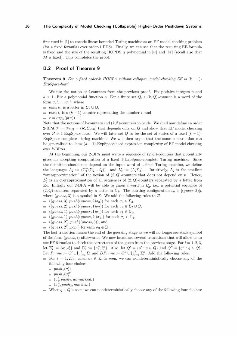
We now define the formula Equalp(n)2 such that, for a reachable configuration c, we have
P2,Q, c |= Equalp(n)2 iff the condition (C2) above is satisfied and that
(C1’) top2 has a prefix of the form σ3vγ3vβ3, where σ3, γ3, β3 ∈ Σ3 and v a 2-counter.To define this formula, we first define the formula 2Counter2 which expresses that top2 hasa prefix of the form σ3vγ3uβ3, where v and u are (not necessarily the same) 2-counters.This can be done in the same way as we defined Counterp(n)
2 , i.e., we need to place anothermarking σ′′3 ∈ Σ′′3 immediately after the previous 2-counter. Assuming 2Counter2 is satisfied,to violate Equalp(n)
2 , we will locate a position (i.e. 1-counter) inside v and show that thecorresponding position in u contains a different symbol. In order to pick a position, we willuse the technique of “marking” used for defining Counterp(n)
Here, Rightposn makes sure that we are in the right position:
Check2 ∧ EX[Σ′2 ∪Q′]AG(¬(Σ′′2 ∨Q′′)).
This makes sure that we are still inside the current 2-counter v and that we did not marksymbols in Σ2 ∪Q in the process (i.e. not replace them by symbols in Σ′′2 ∪Q′′). We shallnow mark the current top1 symbol and mark the corresponding position in u. Therefore, θ′is the following formula
Here, Rightposn′ makes sure that we are in the right position, i.e., it’s a conjunction of thefollowing formulas:
That we are inside u (it is a modification of Check2):
EX[Σ′2 ∪Q′] EFΣ′′3 ∧ ¬EF (Σ′′3 ∧ EXEFΣ′′3)∧
EF (Σ′3 ∧ EFΣ′′3)∧¬EF (Σ′3 ∧ EXEF (Σ′3 ∧ EFΣ′′3))
.
The first three conjuncts ensure that we have passed the symbol γ3 ∈ Σ3. The lastconjunct ensures that we have not passed the conjunct β ∈ Σ3. The reasoning is similarto how we define the formula Check2.That there is only one 1-store below the topmost 1-store satisfying Σ′′2 ∪ Q′′, i.e., theposition that we marked in θ′:
Now, the formula θ′′ will mark the current position and check that the two marked positionsare the same and the corresponding content of the position (i.e. two symbols from Σ′′2 ∪Q′′)are also the same:
EX[Σ′′2 ∪Q′′]Equal′1 ∧ ∨
α′′∈Σ′′2∪Q′′(α′′ ∧ EFα′′)
.
20 The Complexity of Model Checking (Collapsible) Higher-Order Pushdown Systems
Here, the second conjunct tests that the contents are indeed the same. Here, Equal′1 isan easy modification of Equalp(n)
1 which tests that the two positions marked (i.e. they are1-counters) are the same.
Likewise, we can define a formula Succp(n)2 such that, for a reachable configuration c, we
have P2,Q, c |= Succp(n)2 iff the condition (C2) above is satisfied and that
(C3’) top2 has a prefix of the form σ3vγ3uβ3, where σ3, γ3, β3 ∈ Σ3 and v, u are two suc-cessive 2-counters.
Now, we are ready to show that the expression complexity of EF is 1-ExpSpace-hard.Let us take a fixed exponential space bounded, say exp1(p(n)), Turing machine T with statesQ. Our fixed 2-BPA is then P2,Q. Combining the technique that we use for establishinglower bounds for data complexity of EF over HOPDS in the previous subsection and theformulas Counterp(n)
i , Lastp(n)i , Firstp(n)
i , Equalp(n)i that we just defined, it is not hard to
reduce membership of T to model checking EF over P2,Q. There are three extra things thatwe will have to ensure, which can be done easily:
The bottomost configuration guessed is an initial configuration. That is, it contains anencoding of q0w followed by exp1(p(n))− n blank symbols.The topmost configuration is an accepting configuration, i.e., it has a final state.In between two consecutive symbols from Σ3 in the initial guess, there is a state symbol,i.e., symbol from Q.
All these can be defined easily in EF using the marking technique that we used to defineCounter
p(n)2 , i.e., we have to mark symbols from Σ3.
Extensions to order-k BPAWe shall briefly sketch this extension to order-3 (this can be easily extended to the gen-eral case in the same manner). The guessing stage can be adapted easily to insteadwrite a sequence of potential (3, Q)-counters on the stack by performing only push1 op-erations as before. The checking stage is also similar. The idea is to create a “stair-of-stairs” structure for the purpose of checking. We shall elaborate more details on this.We will now also use symbols from Σ4, Σ′4 := a′4, b′4, and Σ′′4 := a′′4 , b′′4. When wesee symbols from Σ1 ∪ Σ2, we have the same choices as in our previous construction.On the other hand, when we see a symbol σΣ3 ∪ Σ4 ∪ Q, we can no longer perform(σ′, push2, unmarkedi) and (σ′′, push2,markedi) operations, but instead we can use theoperations (σ′, push3, unmarkedi) and (σ′′, push3,markedi) (where i is one of 3, 4, Q as be-fore). In this way, we are building a 3-store whose 2-stores (except the topmost) displaysthe projection of a prefix of the guessed configuration [w]3 onto Σ3∪Σ4∪Q as top1 symbols.Note that we use Σ3 for displaying tape contents of the Turing tape, Q as the states of theTuring machine, and Σ4 as separators of two consecutive configurations. Also, note thateach 2-counter encoding the address of a cell position can be doubly exponentially large andare displayed inside each 2-store (in the same way as the previous construction).
B.3 Proof of Theorem 10
Theorem 10. For a fixed formula, model checking CTL over a given order-k HOPDS withoutcollapse is k-ExpTime-hard.
Given an alternating order-(k−1) pushdown automaton P augmented with an s(n)-spacebounded two-way work tape, we show that the membership problem can be polynomially
M. Hague and A. W. To 21
reduced to the satisfaction of a fixed CTL formula ϕ by an order-k pushdown system PwP .Here, we take s(n) to be a polynomial.
The reduction is similar to that used by Bozzelli for CTL model checking of pushdownsystems [4] and borrows further ideas from Engelfriet [13].
The idea of the reduction is as follows: an order-k stack is used to navigate a computationtree of the order-(k− 1) alternating HOPDA in a standard way. To simulate the work tape,at each step, after simulating an operation on the order-(k − 1) stack, a sequence of s(n)work tape symbols (with the head position marked) are pushed on to the top order-1 stack.After this is done, the system can either check that the guessed work tape is consistent withthe previous tape, or continue the execution. To continue the execution, an order-k pushoperation saves the current state (for backtracking), then the work tape is erased. Thisprocess repeats. When an accepting configuration is seen, or the children of the currentnode have been fully explored, the automaton backtracks, and checks untested universalbranches. The automaton accepts when the empty stack is reached. That is, all paths havebeen explored, and found to be accepting.
The CTL formula asserts that a path encoding an accepting tree exists, and that afterguessing the work tape, the branches checking consistency all accept. The formula is
ϕ = E ((op ∧AX(check → AFgood))Ufin)
where op indicates the current path is simulating a tree, and check indicates a consistencychecking branch. The proposition good indicates that the check has been passed, and findenotes the (successful) completion of the run.
I Definition 17. Given a word w of length n and an alternating order-(k − 1) pushdownautomaton P augmented with an s(n)-space bounded two-way work tape, we define theorder-k pushdown system PwP . We assume without loss of generality that two rules can beapplied from each configuration, and which can be referred to as the first and second rulesrespectively. We also assume the initial state is existential. Finally, let 2 denote an emptywork tape cell, and ⊥P denote the bottom of stack character for P.
We define PwP to have the following transitions. The set of states is defined implicitly.The initial state is init. To initialise the automaton we have
(init,⊥, (pushfin; pushk; pushw), (continue, 0)) where w describes the initial work tape.That is, w = E(2, p0)2s(n)−1# ⊥P .
Note that the pushw erases fin from the copy of the stack created by pushk.The main loop of the simulation is given by the continue states, which have the follow-
ing rules. We store the current word position i on the stack (to aid backtracking) beforeperforming a pushk to continue the execution. The clear phase then removes the currentwork tape from the stack, remembering the important details. We then simulate a movewhich may update the stack. The branch phase is where the automaton can either checkthe consistency of the guessed tape, or continue the execution.
((continue, i), done, pushdone, (back, i))((continue, i), x, (pushix; pushk; pop1), (clear, i, x)) for x ∈ E,A1, A2.((clear, i, x), a, pop1, (clear, i, x)) for all a ∈ ∆ and x ∈ E,A1, A2.((clear, i, x)), (a, p), pop1, (clear, i, x, a, p)) for all a, b ∈ ∆ and p ∈ P and x ∈ E,A1, A2.((clear, i, x, a, p), b, pop1, (clear, i, x, a, p)) for all a, b ∈ ∆ and p ∈ P and x ∈ E,A1, A2((clear, i, x, a, p),#, pop1, (move, i, x, a, p)) for all a ∈ ∆ and p ∈ P and x ∈ E,A1, A2and p is not accepting or i 6= |w|+ 1.((clear, i, x, a, p),#, pop1, (back, i)) for all a ∈ ∆ and p ∈ P and x ∈ E,A1, A2 and pis accepting and i = |w|+ 1.
22 The Complexity of Model Checking (Collapsible) Higher-Order Pushdown Systems
((move, i, x, a, p), γ, (o; pushyw), (branch, r, i)) for all a ∈ ∆, p ∈ P , x ∈ E,A1, A2,γ ∈ Σ. Furthermore when x = E, r is any rule applicable at p, a, γ, w(i); when x = A1,r is the first transition for p, a, γ, w(i); and when x = A2, r is the second transition forp, a, γ, w(i). The operation o is the pushdown operation of r and y is E when r movesto an existential state, and A1 when moving to a universal state. Finally, w is any worktape configuration of length s(n) and with the read head containing state q reached byr. Note that there are an exponential number of w, but we can easily gain all w with alinear number of intermediate states and rules, each guessing the next character of w.((branch, r, i), a, pusha, (continue, j)) where j = i if r is an ε-transition in the input, orj = i+ 1 otherwise; and ((branch, r, i), a, pusha, (check, r)) for all r and a.
The back phase implements the backtracking, and requires the following rules.((back, i), a, popk, (back1, i)).((back1, i), fin, pushfin, fin).((back1, i), j, pop1, (back2, j)).((back2, i), E, pushdone, (continue, i)).((back2, i), A1, pushA2 , (continue, i)).((back2, i), A2, pushdone, (continue, i)).
Finally, the check phase has a branch for all 0 ≤ j ≤ s(n) which ensures the jth positionin the work tape is consistent with the previous work tape, given the rule r has been executed.If there is no previous configuration, the work tape is automatically good.
((check, r), x, pop1, (check, r, j)) for all x ∈ E,A1, A2 and 0 ≤ j ≤ s(n).((check, r, j), a, (pop1)j , (check1, r, j)).((check1, r, j), a, pop2, ((check2, r, j, a)).((check2, r, j, a), fin, pushfin, good).((check2, r, j, a), x, (pop1)j+1, (check3, r, j, a)) if a is not a pair (b, q), and also the rules((check3, r, j, a), b, pushb, good) where b = a or b = (b′, q) where r reads b′ at state q andwrites a to the tape.((check2, r, j, (a, q)), x, (pop1)j , (checkL, r, j, (a, q))) if r moves left, q is moved to by r,and ((checkL, r, j, (a, q)), (b, q′), pop1, (check′L, r, j, (a, q))) where q is moved from by r andb is read by r. Finally, we have the following rule ((check′L, r, j, (a, q)), a, pusha, good).((check2, r, j, (a, q)), x, (pop1)j+1, (checkR, r, j, (a, q))) if r moves right, q is moved to by r,and ((checkR, r, j, (a, q)), a, pop1, (check′R, r, j, (a, q))). Finally, we have additional rules((check′R, r, j, (a, q)), (b, q′), push(b,q′), good) where b is read by r and q′ is moved from byr.
The atomic proposition op is true during the init, continue, clear, move, branch and backphases. The proposition check is true during the check phase, good true at state good andfin at state fin.
I Property 1. A word w is accepted by P iff PwP satisfies the fixed formula ϕ. Furthermore,PwP is polynomial in the size of w and P.I Corollary 18. CTL model checking of order-k pushdown systems is k-ExpTime-hard, evenfor a fixed formula ϕ.
Proof. Take any language L in⋃d>0 DTIME(expk(ds(n))) for some polynomial s(n). There
exists a Turing machine M such that M accepts a word w iff w ∈ L. From Theorem 5 weknow that there is an order-(k−1) alternating pushdown automaton PM with an s(n)-spaceauxiliary work tape such that w ∈ L iff w is accepted by P. Then, by Property 1, we have,by a polynomial reduction, that w ∈ L iff PwP satisfies ϕ. J
M. Hague and A. W. To 23
B.4 Proof of Theorem 11
Theorem 11. For a fixed order-k HOBPA without collapse, model checking CTL is k-ExpTime-hard.
We adapt the reduction for CTL to give a k-ExpTime expression complexity for CTLover HOBPA.
I Definition 19. Given an alternating order-(k−1) pushdown automaton P augmented withan linear-space bounded two-way work tape, we define the order-k pushdown system PP .We assume without loss of generality that two rules can be applied from each configuration,and which can be referred to as the first and second rules respectively. We also assume theinitial state is existential. Since there is only one control state, we write (a, o) instead of(q, a, o, q) where o is a pushdown operation. Finally, let 2 denote an empty work tape cell,and ⊥P denote the bottom of stack character for P.
Note, the format of the tape simulation information on the stack is a string, for example,E0101ab(c, p)d# to indicate an existential position, and word position 0101 with cell contentsab(c, p)d. The structure of the whole stack is an sequence of (k− 1) stacks. The top (k− 1)stack represents the current configuration being simulated. The next (k − 1) stack simplycontains, on its top character, a representation of the rule r used to reach the configuration.The (k − 1) stack underneath is the previous configuration, and so on.
We define PP to have the following transitions. The set of states is defined implicitly.To initialise the automaton we have the following rules. Since we cannot use a control state,these rules take care of adding work tape and simulation information to the stack in general.We use the formula to assert a correct flow. For every character x, we also use x to indicatethat the character has been reached via a pop operation.
(⊥, (fin; pushk;⊥′)) and (⊥′, push#⊥P ).(#, pushc#), (c, pushc′c) where c, c′ ∈ ∆ ∪ (∆× P ).(c, pushic), (i, pushi′i) where i, i′ ∈ 0, 1 and c ∈ ∆ ∪ (∆× P ).(i, pushxi) where i ∈ 0, 1 and x ∈ E,A1,X.After writing the work tape we have E,A1 or X on the stack, we continue the execution
with a pushk or check the contents of the work tape. Alternatively, if we reach x forx ∈ E,A1, A2 then we are either checking the tape or backtracking, hence we announcewhich before continuing appropriately.
(x, (x; pushk; continue)) where x ∈ E,A1 and (A1, (A2; pushk; continue)).(x, push(x,check)) where x ∈ E,A1, A2,X.(x, pushcheck2) where x ∈ E,A1, A2,X.(x, pushback) where x ∈ E,A2,X
.
(back, popk) and (y, pop1) for y ∈ continue, (x, check), check2.(x, pop1) for all x 6= #.(#, pushmove), (#, pushpop).(pop, popk), (r, popk) for all rules r.(move, pop1).
To simulate a move we first announce on the stack which move will be executed. Thenwe copy the stack to remember the move joining the configurations. Then we fire the ruleand continue the execution. Let op(r) be the stack operation of the rule r and top(r) be thetop of stack character after the rule has fired (which can be obtained from the rule alone),if the rule is a push rule.
24 The Complexity of Model Checking (Collapsible) Higher-Order Pushdown Systems
(c, push(c,r)), ((c, r), (r; pushk; (c, r)′)).((c, r)′, (c; op(r); (top(r), done)), ((c, done), push#)c) when op(r) is a push rule, and((c, r)′, op(r)), (a, push#a) when op(r) is a pop rule and a is a stack character from thesimulated HOPDA.
We define propositions to be true when forming part of the top of stack character. Forexample x will be true when x, x or (x, y) are on the top of the stack. We also use op toindicate all states that are not check declarations.
The corresponding CTL formula is defined below.
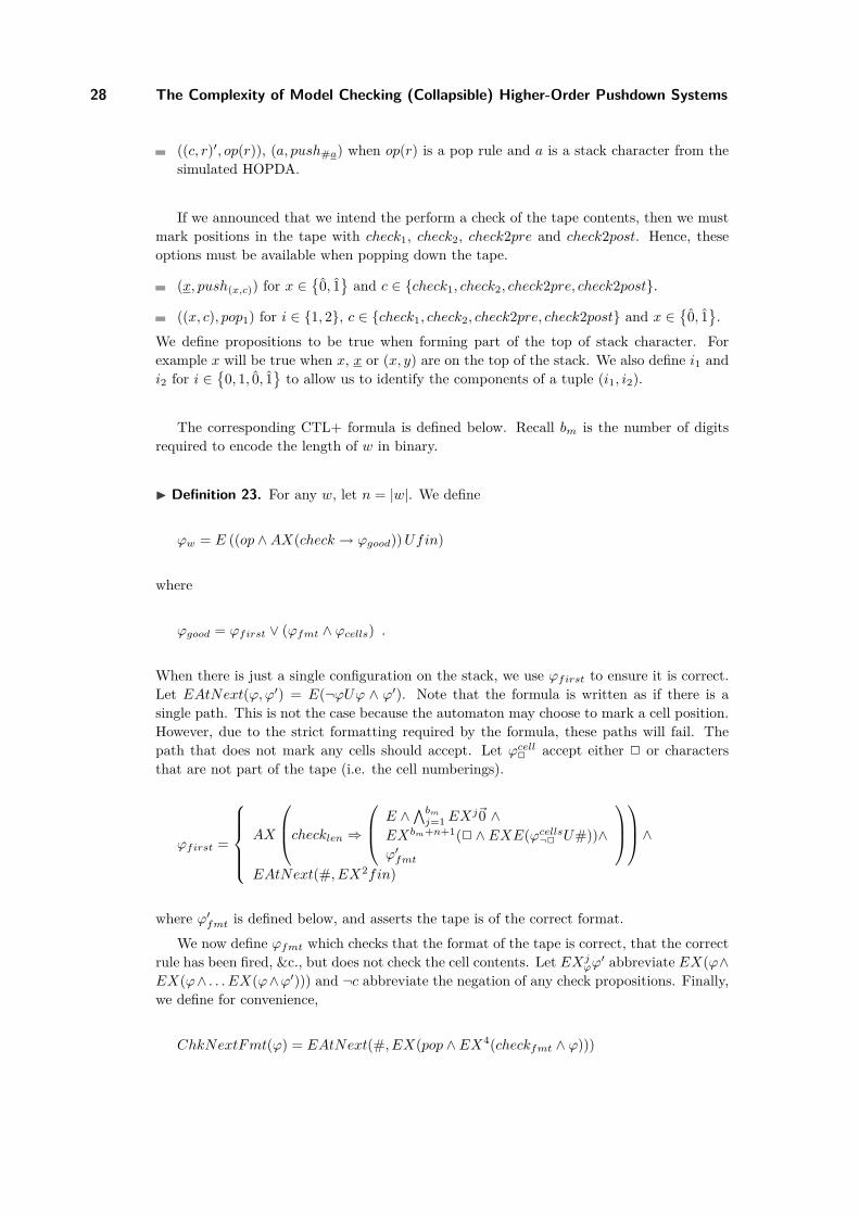
I Definition 20. For any w, let n = |w|. We define
ϕw = E ((op ∧AX(check → ϕgood))Ufin)
where ϕgood is of the form
ϕgood = ϕfirst ∨ (ϕAE ∧ ϕfmt ∧ ϕi ∧ ϕr ∧ ϕtape)where each component formula is defined below. Let Bin(i, bm)(j) be the jth bit of thebinary encoding of i. To ease readability we define EAtNext(ϕ,ϕ′) = E((¬ϕ)U(ϕ ∧ ϕ′)).That is, at the next time ϕ is true, ϕ′ is also true. We also define ChkNext(ϕ) that looksinto the next work tape on a check branch and Rule(r) that is used to match the rule rconnecting the configurations. That is,
ChkNext(ϕ) = EAtNext(#, EX
(pop ∧ EX3 (check2 ∧ ϕ)
))Rule(r) = EAtNext (#, EX (pop ∧ EXr)) .
When there is just a single configuration on the stack, we use ϕfirst to ensure it is correct.Note that, given a correct initialisation, ϕtape (defined below) ensures the tape format iscorrect in following configurations.
ϕfirst =
E ∧∧bmj=1EX
j0 ∧ EXbm+1(2, p0)∧s(n)j=1 EX
bm+j2∧EXbm+s(n)+1# ∧ EXbm+s(n)+4fin
.
For the remaining positions ϕAE ensures the placement of E,A1, A2 and X is correct.Let ϕtox for x ∈ E,A1, A2,X denote the disjunction of all rules of leading to a state oftype x.
ϕAE =∨
x∈E,A1,A2,Xx ∧ EAtNext (#, EX (pop ∧ EXϕtox ))
The formula ϕfmt ensures the topk stack has yBin(i, bm)w# as the beginning of the firsttwo top1 stacks, where y ∈ E,A1, A2 and w is a work tape of length s(n).
ϕ′fmt =(∧bm
j=1EXj(0 ∨ 1)
)∧(∧s(n)
j=1 EXbm+j ∨
a,(p,a)(a ∨ (p, a)))
ϕfmt = ϕ′fmt ∧ ChkNext(ϕ′fmt) .The next formula ϕi ensures that the input position counter is consistent with the previouscounter. Note that this will ensure, when backtracking to a universal position, the secondbranch will have the same counter as the first: both must be consistent with the ancestor’scounter.
ϕi =∧r
Rule(r)⇒ EXϕri
M. Hague and A. W. To 25
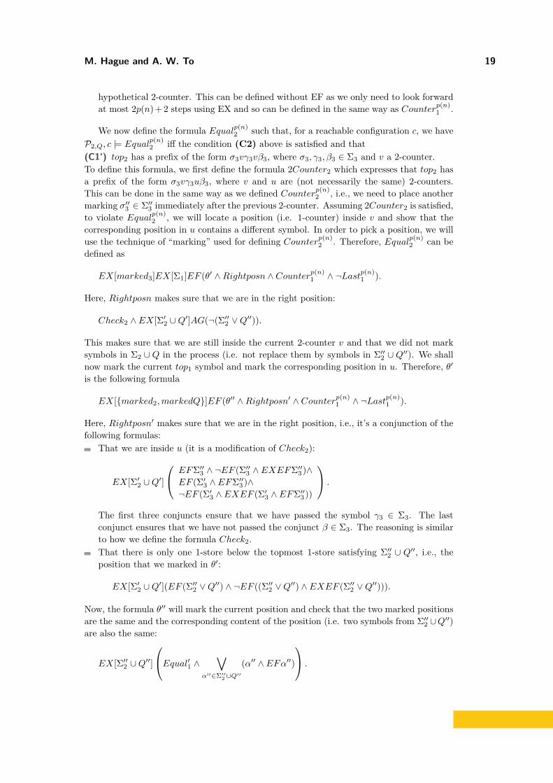
Furthermore, if r is an ε-transition, we define
ϕri =∨nj=0Num(j) ∧ ChkNext(EXNum(j))
Num(j) =∧bm−1j′=0 EXj′Bin(j, bm)(j′)
otherwise
ϕri =n∨j=1
(Num(j)∧ChkNext(EXNum(j − 1))
).
The formula ϕr asserts that the applied rule r matches the claimed input positions. Letinp(r) denote the input character associated with a rule r.
ϕr =∨r Rule(r)⇒
∨inp(r)=w(j) ChkNext(EXNum(j)) .
Finally, ϕtape ensures that the tape contents have been updated accurately. We use, forshorthand, functions Nextr(σ1, σ2, σ3) = d that specifies the contents of the current (jth)cell d with respect to the rule fired r and the contents of the previous configuration’s (j−1)th,jth and (j + 1)th cells σ1, σ2 and σ3 respectively. Let #l and #r denote, for the benefit ofNextr(σ1, σ2, σ3), the left and right boundaries of the tape respectively.
I Property 2. A word w is accepted by P iff PP satisfies the formula ϕw. Furthermore, PPand ϕw are polynomial in the size of w and P.I Corollary 21. CTL model checking of fixed order-k HOBPA is k-ExpTime-hard.
Proof. Take any language L in⋃d>0 DTIME(expk(ds(n))) for some polynomial s(n). There
exists a Turing machine M such that M accepts a word w iff w ∈ L. From Theorem 5 weknow that there is an order-(k−1) alternating pushdown automaton PM with an s(n)-spaceauxiliary work tape such that w ∈ L iff w is accepted by P. Then, by Property 2, we have,by a polynomial reduction, that w ∈ L iff PP satisfies ϕw. J
C Proof of Theorem 12
Theorem 12. For a fixed order-k HOBPA without collapse, model checking CTL+ is(k + 1)-ExpTime-hard.
We adapt the reduction for CTL to give an (n + 1)-EXPTIME expression complexityfor CTL+ over HOBPA. Will begin with an informal description of the proof for CTL* andexplain how to adapt it for CTL+.
The reduction we use to show CTL* is (k + 1)-ExpTime-hard over order-n pushdownsystems is similar to Bozzelli’s proof for the order-1 case. In fact, only a simple adjustment
26 The Complexity of Model Checking (Collapsible) Higher-Order Pushdown Systems
to the HOPDS construction for the k-ExpTime-hard result of CTL has to be made. Themain technical steps of the proof are in the definition of the required CTL* formula, whichwas already given by Bozzelli.
We reduce from an order-(k − 1) alternating HOPDA with an exponential space worktape. The order-k PDS we construct manages the alternation in the same manner as thereduction for CTL. The only difference is in the generation of work tapes. For the CTLreduction we could simply output a polynomial number of tape symbols, and check forconsistency using only a polynomial number of states. However, the same strategy foran exponential space bounded tape would require an exponential number of states. Thetrick is to output an arbitrary length tape, and use the power of CTL* to reject any tapeconfigurations that are not exponential.
In more detail, the HOPDS represents tape configurations as words of the form
binn(0)c0binn(1)c1 · · · binn(2n − 1)c2n−1
where binn(i) is the n-digit binary representation of i with the least significant bit first. Itis beyond the power, however, of a polynomially sized HOPDS to output only sequencesthat count correctly from 0 to 2n − 1. Hence, the HOPDS generates, nondeterministically,a word of the form
(0, 1n (∆ ∪ (∆×Q)))∗ .
One can check whether a configuration of this form is of the correct length as follows: firstassert that the first n-digit binary number is 0n. Then check that every pair bicibi+1ci+1has bi = bi+1 + 1. Finally, the last number must be all 1s.
The checking phase of the HOPDS now proceeds as follows. One branch simply popsthe configuration from the stack. This branch allows the CTL formula to check the lengthof the configuration.
The remaining branches remove the tape configuration from the stack, but nondeter-ministically mark one position with the proposition check1 (hence there are a number ofbranches for this step). Next popks are performed to retrieve the previous work tape. Thenthe HOPDS does the same as before: pops the tape from the stack, nondeterministicallymarking a position with check2. The CTL* formula can test consistency by checking whetherthe two positions correspond to the same position in the work tape. If so, the markers check1and check2 can be used to test the contents of the cell (and it’s neighbours) to ensure a validupdate has taken place.
To refine the construction to show CTL+ is (k + 1)-ExpTime-hard over order-k push-down systems, the key restriction of CTL+ that has to be overcome is that the CTL*formulas may contain nested path operators within a single path quantification. We over-come this adding extra marking information to the HOPDS. For example, we avoid the needto count (n + 2) steps ahead when comparing one cell position with the next by adding acheck2pre and a check2post marker into the HOPDS. That is, before marking the check2position, the automaton will place a check2pre on the preceding tape character. Then, afterplacing check2, check2post will be placed on the next tape character.
In the case of HOBPA, it is not possible for the system to enforce the expected placing ofthe propositions check2pre, check2 and check2post. That is, we can use the until operatorto ensure that the propositions appear in order ((¬check2Ucheck2pre)) but cannot enforcethat they appear in adjacent cells.
The trick is to encode cell numberings as sequences of tuples (b1j , b2j ) such that the encodednumbers differ by one. That is b2 + 1 = b1. We can then ensure that the three propositions
M. Hague and A. W. To 27
are on adjacent cells in the same way we ensured check1 and check2 are on correspondingcells. Recall that all binary numbers are encoded with the least significant digit first.
The cost of this encoding is that our work tape will contain 2n−2 cells, but this is clearlynot a problem for the complexity result.
I Definition 22. Given an alternating order-(k − 1) pushdown automaton P augmentedwith an 2n-space bounded two-way work tape, we define the order-k pushdown system PP .We assume without loss of generality that two rules can be applied from each configuration,and which can be referred to as the first and second rules respectively. We also assume theinitial state is existential. Since there is only one control state, we write (a, o) instead of(q, a, o, q) where o is a pushdown operation. Finally, let 2 denote an empty work tape cell,and ⊥P denote the bottom of stack character for P.
Note, the format of the simulation information on the stack is, for example,
to indicate an existential position, and word position ~0~1~0~1 with cell contents ab . . ..We define PP to have the following transitions. The set of states is defined implicitly.
The initial state is init. To initialise the automaton we have the following rules. Sincewe cannot use a control state, these rules take care of adding work tape and simulationinformation to the stack in general. We use the formula to assert a correct flow.
(⊥, (fin; pushk;⊥′)) and (⊥′, push#)⊥P ).(#, pushc#), (c, pushic), where i ∈ 0, 12 and c ∈ ∆ ∪ (∆× P ).(i, pushi′i) where i ∈ 0, 12 and i′ ∈ 0, 12 ∪ 0, 12.(i, pushci) where i ∈ 0, 12 and c ∈ ∆ ∪ (∆× P ).(c, pushic), (i, pushi′i) where i, i′ ∈ ~0,~1 and c ∈ ∆ ∪ (∆× P ).(i, pushxi) where i ∈ ~0,~1 and x ∈ E,A1,X.After writing the work tape we have E,A1 or X on the stack, we continue the execution
with a pushk or check the contents of the work tape. Alternatively, if we reach x forx ∈ E,A1, A2 then we are either checking the tape or backtracking, hence announcewhich before continuing appropriately.
(x, (x; pushk; continue)) where x ∈ E,A1,X and (A1, (A2; pushk; continue)).(x, push(x,check)) for x ∈ E,A1, A2,X, E,A1, A2
.
(x, pushback) for x ∈ E,A2,X.((x, check), push(x,checkfmt)), ((x, check), pushcheckcells) for x ∈ E,A1, A2,X.(y, pop1) for y ∈ continue, (x, checkfmt), checkcells.(back, popk).(x, pop1) for all x 6= #.(#, pushmove), (#, pushpop).(pop, popk) and (r, popk) for all rules r.(move, pop1).
To simulate a move we first announce on the stack which move will be executed. Then wecopy the stack to remember the move joining the configurations. Then we fire the rule andcontinue the execution. Let op(r) be the stack operation of the rule r and top(r) be the topof stack character after the rule has fired (which can be obtained from the rule alone), if therule is a push rule.
(c, push(c,r)), ((c, r), (r; pushk; (c, r)′)).((c, r)′, (c; op(r); (top(r), done)), ((c, done), push#)c) when op(r) is a push rule, and
28 The Complexity of Model Checking (Collapsible) Higher-Order Pushdown Systems
((c, r)′, op(r)), (a, push#a) when op(r) is a pop rule and a is a stack character from thesimulated HOPDA.
If we announced that we intend the perform a check of the tape contents, then we mustmark positions in the tape with check1, check2, check2pre and check2post. Hence, theseoptions must be available when popping down the tape.
(x, push(x,c)) for x ∈ 0, 1 and c ∈ check1, check2, check2pre, check2post.((x, c), pop1) for i ∈ 1, 2, c ∈ check1, check2, check2pre, check2post and x ∈
0, 1.
We define propositions to be true when forming part of the top of stack character. Forexample x will be true when x, x or (x, y) are on the top of the stack. We also define i1 andi2 for i ∈ 0, 1, 0, 1 to allow us to identify the components of a tuple (i1, i2).
The corresponding CTL+ formula is defined below. Recall bm is the number of digitsrequired to encode the length of w in binary.
I Definition 23. For any w, let n = |w|. We define
ϕw = E ((op ∧AX(check → ϕgood))Ufin)
where
ϕgood = ϕfirst ∨ (ϕfmt ∧ ϕcells) .
When there is just a single configuration on the stack, we use ϕfirst to ensure it is correct.Let EAtNext(ϕ,ϕ′) = E(¬ϕUϕ ∧ ϕ′). Note that the formula is written as if there is asingle path. This is not the case because the automaton may choose to mark a cell position.However, due to the strict formatting required by the formula, these paths will fail. Thepath that does not mark any cells should accept. Let ϕcell2 accept either 2 or charactersthat are not part of the tape (i.e. the cell numberings).
ϕfirst =
AX
checklen ⇒ E ∧∧bmj=1EX
j~0 ∧EXbm+n+1(2 ∧ EXE(ϕcells¬2 U#))∧ϕ′fmt
∧
EAtNext(#, EX2fin)
where ϕ′fmt is defined below, and asserts the tape is of the correct format.We now define ϕfmt which checks that the format of the tape is correct, that the correct
rule has been fired, &c., but does not check the cell contents. Let EXjϕϕ′ abbreviate EX(ϕ∧
EX(ϕ∧ . . . EX(ϕ∧ϕ′))) and ¬c abbreviate the negation of any check propositions. Finally,we define for convenience,
and ϕAE ensures the placement of E,A1, A2 and X is correct. Let ϕtox for x ∈ E,A1, A2,Xdenote the disjunction of all rules of leading to a state of type x.
ϕAE =∨
x∈E,A1,A2,Xx ∧ EAtNext (#, EX (pop ∧ EXϕtox ))
and ϕi checks that the word positions are updated correctly.
ϕi =∧r Rule(r)⇒ EXϕri
Num(j) =∧bmj′=0EX
j′Bin(j, bm)(j′)
and, if r is an ε-transition, then
ϕri =n∨j=0
Num(j) ∧ ChkNextFmt(EXNum(j))
and otherwisen∨j=1
Num(j) ∧ ChkNextFmt(EXNum(j − 1))
The next formula ϕr ensures that the fired rule is applicable at the current word position.Let inp(r) denote the input character associated with a rule r.
ϕr =∨r Rule(r)⇒
∨inp(r)=w(j) ChkNextFmt(EXNum(j)) .
Finally ϕcells takes advantage of the fact that there is no branching while popping binaryblocks to avoid nesting temporal operators.
where θ1 asserts that the checks are placed correctly, and θ2 tests the consistency of thetape. As well as asserting that the propositions are in the right position, θ1 must also assert
30 The Complexity of Model Checking (Collapsible) Higher-Order Pushdown Systems
that there is only one copy of each check proposition. We require check2pre and check2postto hold at the beginning of the binary blocks.
)To define θ2, we use, for shorthand, functions Nextr(σ1, σ2, σ3) = d that specifies the
contents of the current (jth) cell d with respect to the rule fired r and the contents of theprevious configuration’s (j − 1)th, jth and (j + 1)th cells σ1, σ2 and σ3 respectively. Let #l
and #r denote, for the benefit of Nextr(σ1, σ2, σ3), the left and right boundaries of the taperespectively.
F (check2pre ∧ EXnσ1)∧F (check2 ∧ EXnσ2)∧F (check2post ∧ EXnσ3)
→ Nextr(σ1, σ2, σ3)
θrl =∨σ1,σ2
(F (check2pre ∧ EXnσ1)∧F (check2 ∧ EXnσ2)
)→ Nextr(σ1, σ2,#r) .
I Property 3. A word w is accepted by P iff PP satisfies the formula ϕw. Furthermore, PPand ϕw are polynomial in the size of w and P.I Corollary 24. CTL model checking of fixed order-k HOBPA is (k + 1)-ExpTime-hard.
Proof. Take any language L in⋃d>0 DTIME(expk+1(ds(n))) for some polynomial s(n).
There exists a Turing machineM such thatM accepts a word w iff w ∈ L. From Theorem 5we know that there is an order-(k − 1) alternating pushdown automaton PM with an 2n-space auxiliary work tape such that w ∈ L iff w is accepted by P. Then, by Property 3, wehave, by a polynomial reduction, that w ∈ L iff PP satisfies ϕw. J
D Proofs For Linear Time
D.1 Proof of Theorem 13
Theorem 13.Model checking µLTL against order-k CPDSs is in k-ExpTime for a non-fixedformula, and (k − 1)-ExpTime for a fixed formula.
M. Hague and A. W. To 31
It is well known that any formula of µLTL has a Büchi automaton representation. Weform the product of the CPDS and the Büchi automaton corresponding to the negationof the µLTL formula ϕ. This gives us a Büchi CPDS; that is, a CPDS with a set F ofaccepting control states. Thus, model checking reduces to the non-emptiness problem forBüchi CPDSs.
The non-emptiness problem for Büchi CPDSs is a special case of determining the winnerin a parity game played over a CPDS. In particular, it is a single-player game with a fixednumber (two) of colours. It is known that an order-k game can be reduced to an order-(k−1) game with an exponential blow-up [17]. This leads to a recursive algorithm resultingin a finite-state parity game of k-exponential size, and since known finite-state algorithmsare polynomial in the number of states (and exponential in the number of colours), thealgorithm runs in k-ExpTime.
We demonstrate, in this simple case, the single-player order-k game can be reduced toa two-player order-(k − 1) game with only a polynomial blow-up. This order-(k − 1) gameis then solved as above, giving, an overall algorithm in (k − 1)-ExpTime in the size of theBüchi CPDS. That is, (k − 1)-ExpTime for a fixed formula, and k-ExpTime for a non-fixedformula.
We begin by recalling some definitions.
I Definition 25. Let P = (P,R,Σ, p0,⊥) be an order-k CPDS. Then G = (P, PE , PA,Ω) isan order-k CPDS parity game, where PE ] PA = P is a partitioning of the control statesand Ω : P → Col is a function assigning to each control state a colour in the set Col ⊂ N ofcolours.
A play Λ of a parity game between two players, Éloïse and Abelard, proceeds as follows.Play begins with the initial configuration 〈p0, [⊥]k〉. If the control state of the currentconfiguration is is PE , then Éloïse chooses an applicable rule in R. Otherwise Abelardchooses a rule. If a player cannot move, they lose the game. The cycle repeats until a playerloses, or, in the case of an infinite play, the winner is determined by the colouring functionΩ. If the minimal colour occurring infinitely often is even, Éloïse wins the game. OtherwiseAbelard wins.
An important part of the reduction is the notion of collapse rank-aware.
I Definition 26 ([17]). Consider a partial play Λ in G ending in a configuration 〈p, γ〉such that top1(γ) has an k-link. Hence there is in Λ at least one configuration of the form〈p′, collapse(γ)〉 for some p′ ∈ P . Then the closest to 〈p, γ〉 is called the collapse ancestor of〈p, γ〉. The collapse rank of 〈p, γ〉 is the minimal colour of a state occurring in Λ between thecollapse ancestor of 〈p, γ〉 and 〈p, γ〉. Note that these notions are not defined if top1(γ) has aj-link for some j < k: indeed it may happen that no configuration of the form 〈p, collapse(γ)〉was visited in Λ, and therefore the collapse ancestor notion can not be adapted.
I Definition 27 ([17]). An k-CPDS equipped with a colouring function is collapse rank-aware iff there exists a function ColRnk : Σ→ N such that, when defined, the collapse rankof every configuration 〈p, γ〉 is equal to ColRnk(top1(γ)). On other words, the collapse rankis stored in the top1-element of the stack.
Beginning with a Büchi CPDS, we must first make the CPDS collapse rank-aware. Thiscan be done using the following known results. Note that, since both the size of Col and kare fixed, the transformation to a collapse rank-aware CPDS costs only a constant blow up.
I Lemma 28 ([17], Lemma 14, Remark 6.6). For any order-k CPDS P and parity game Gplayed over it, one can construct a collapse rank-aware order-k CPDS P ′ and order-k parity
32 The Complexity of Model Checking (Collapsible) Higher-Order Pushdown Systems
game G′ such that Éloïse wins in G iff she wins in G′. Moreover, P ′ has O(|P ||Col|O(k))control states and a stack alphabet of size O(|Σ||Col|O(k)).
We are now ready to give the main reduction.
I Lemma 29. Given an order-k Büchi CPDS P, one can construct an order-(k− 1) CPDSparity game G of size polynomial in the size of P such that P has an accepting run iff Éloïsewins the game G.Proof. We will describe G somewhat informally. The formal definition should be clear fromthe description. Control states of the game are of the form (p, pr, f) for control states p andpr and the boolean flag f . We also allow pr = null. Intuitively, p is the current controlstate of the configuration being simulated, pr is a promise to reach the control state pr whena popk, and f is an obligation to visit a final state before the popk. Similarly, the stackcharacters are either simply characters a, or, when simulating a character with a k-link, ofthe form (a, pr, f), which play the same role as (p, pr, f) does, but in the case of a collapseover a k-link.
We describe how each rule application is simulated. Except when stated, Éloïse makesall moves. Consider the rule (p, a, o, p′). In cases:
When o is a pushdown command that is not pushk, popk, pushka, or collapse when thetop1 character contains a k-link, the simulation is direct: o is simply applied and wereach the control state (p′, pr, f ′) where f ′ is true iff f is true and p was not final.When o is popk, play proceeds to a winning (sink) state for Éloïse if p′ = pr and f isfalse. Otherwise we reach a winning state for Abelard. The stack is not changed.When o is collapse and the top1 character is (p, pr, f), play proceeds to a winning (sink)state for Éloïse if p′ = pr and ColRnk(p, pr, f) indicates a final state has been seen if fis true. Otherwise we reach a winning state for Abelard. The stack is not changed.When o is pushk, Éloïse declares a pair p′r and f ′, indicating that, when the order-(k−1)stack to be created is finally popped (if it is popped), then play will reach the state p′r,and f ′ indicates whether a final state will have been seen on the way. Abelard can acceptthe declaration and move play to (p′r, pr, f ′′) without changing the stack, where f ′′ istrue only if f is true and f ′ is not. Alternatively, Abelard may question the declarationand move play to (p′, p′r, f ′) (without changing the stack).When o is pushka we proceed as follows. We apply push1
(a,pr,f) and move to (p′, pr, f).The idea is that Éloïse’s commitments are saved to the stack in place of the k-link. Iffollowing the collapse link is simulated, it must be in line with her previous declarations.
The final states are all control states where the first component p is final in the originalgame. It is also the case that, when Abelard accepts a declaration by Éloïse that she canpass through a final state, we ensure that, in the simulation, an intermediate final state ispassed through. The initial state is (p, null, false) and stack bottom is ⊥.
Observe that, since there are no order-k stack operations in the simulation, the resultinggame is order-(k − 1).
To see why the simulation is correct, first consider an accepting run of the Büchi CPDS.At each pushk, then either the current stack contents appear again on the run, in whichcase Éloïse simply declares the control state at this return, and whether a final state wasencountered en-route. Otherwise, she declares null and play proceeds to simulate the pushk.Since the stack contents below the new top stack are never encountered again, they can besafely forgotten.
In the other direction, take a winning strategy for Éloïse. This strategy can be linearised,constructing a run as follows: at each pushk, play has two branches. On the first, Abelard
M. Hague and A. W. To 33
questions Éloïse’s declaration, on the second, he accepts it. We recursively compute the runfrom the first branch and append to it the run from the second branch. This leads to aninfinite run with a infinite number of final states seen. J
D.2 Proof of Theorem 15
Theorem 15. Model checking LTL(F, X) and LTL(U) against a fixed HOBPA withoutcollapse is k-ExpTime-hard.
We give proofs for the two logics in turn.
D.2.1 Lower Bound for LTL(F, X)Given a fixed k-EXPTIME complete language L, Theorem 5 implies that there exists a fixedorder-k pushdown automaton P = (P,R,Σ,Γ ∪ ε ,∆, p0,⊥,F) augmented with an s(n)-space bounded two-way work tape that accepts precisely the language L from 〈p0, [⊥]k〉. Wenow construct an order-k BPA P ′ = (R′,Σ, c′0) and later show that there is a reduction ofthe membership problem for L(P) to LTL model checking over P ′, which shall imply thatexpression complexity of order-k BPA is k-ExpTime-hard.
Let ∆′ = ∆× h, h (h stands whether head is in this position or not). For an alphabetΩ, we let Ω? = Ω ∪ ? assuming that ? /∈ Ω. Similarly, we let Ω# be Ω ∪ # assumingthat # /∈ Ω. Let W = R ∪ sink. Let Σ′ = (P? ×W? × Σ) ∪ Σ ∪ (Σ × ∆′). The initialconfiguration c′0 is 〈[(p0, ?,⊥)]k〉. We now add the following rules to R′:1. for each p ∈ P , a ∈ Σ, and r ∈ R where r is of the form ((p, ∗, a, ∗), o, ∗)1, add
((p, ?, a), push(p, r, a)).
and add
((p, r, a), fa(o)).
where fa : Ok → Ok is defined as fa(o′) = o′, if o′ ∈ O1 or of the form popj , andfa(o′) = (pusha; pushj ; pusha), if o′ = pushj for some j > 1.
2. for each a ∈ Σ and x ∈ ∆′, add (a, push((a, x))).3. for each x, y ∈ ∆′ and a ∈ Σ, add ((a, x), push((a, y))).4. for each x ∈ ∆′ and p ∈ P , add ((a, x), push((p, ?, a))).5. we add “sink” transitions: ((p, ?, a), push(p, sink, a)) and ((p, sink, a), push(p, sink, a))
for any p ∈ F and a ∈ Σ.Intuitively, each run of P ′ will have valuations of the form
We will now enforce the correct form via LTL formulas.
1 Here, we use the wildcard ∗ to match a symbol or a tuple of symbols.
34 The Complexity of Model Checking (Collapsible) Higher-Order Pushdown Systems
Given a word w = α1 . . . αn ∈ Γ∗, we now construct an LTL formula ϕw using only Fand X temporal operators such that w ∈ L(P) iff P ′, c′0 6|= ¬φw. We first define a formulaψ that makes sure that precisely the word w is consumed during a guessed run:
ψ = ψ1 ∧ ψ2 ∧ ψ3.
Let V be precisely the subset of P × R × Σ, where the rule component is of the followingform ((∗, α, ∗, ∗), ∗, ∗), for some α ∈ Γ; in other words, these are rules which “consume” aninput letter. The formula ψ1 states that at least n letters are consumed in the run; let
ψ01 := True
ψi+11 := XF (V ∧ ψi1)ψ1 := ψn1 .
The formula ψ2 states that at most n letters are consumed in the run:
ψ2 := ¬ψn+11 .
To define ψ3, let Vα be subset of V where the rule component is the form ((∗, α, ∗, ∗), ∗, ∗).The formula ψ3 states that the ith letter consumed in the run is wi:
ψ03 := True
ψi+13 := XF (Vαn−i+1 ∧ ψi3)ψ3 := ψn3 .
We now ensure that after each occurrence of (P ×R × Σ) in the run (as in (*) and (**)),we see precisely a stack symbol in Σ, followed by precisely s(n) symbols from Σ×∆′, whichare in turn followed by a symbol (p, ?, a) of the “right” form. Notice that this would meanthat we may partition each run as a contiguous sequence of blocks of size m := 3 + s(n)according to (*) and (**). More formally, define θ as follows:
θ :=∨
(p,r,a)∈P×R×Σ
G((p, r, a)→ P × ? × Σ.
If r is not of the form ((p, ∗, a, ∗), ∗, ∗), then we define θ(p,r,a) = False. Otherwise, lettingr = ((p, ∗, a, ∗), o, (∗, ∗, p′)), we define θ(p,r,a) as follows:
θ(p,r,a) := (p, r, a) ∧s(n)∧i=1
Xi+1Σ×∆′ ∧Xs(n)+2(p′, ?, a).
Each block of size s(n) (note: Σ is always followed by such a block) encoding the tapecontent needs to have exactly one head:
Onehead := G
Σ→s(n)∨i=1
Headi ∧ ∧1≤j≤s(n),j 6=i
¬Headj ,
where Headj := XjΣ × (∆ × h). Furthermore, two consecutive blocks encoding tapecontents, each of size s(n), must follow in the correct way:
Tapefollow :=∧
(p,r,a)∈P×R×Σ
G((p, r, a)→ XX(s(n)∧i=1
Followi,r)).
M. Hague and A. W. To 35
Here, Followi,r means that the ith cell of the subsequent tape content follows from theith cell of the current tape content using rule r. This formula can be easily defined bynoticing that the ith cell of the subsequent tape content can be uniquely defined fromcells i − 1, i, i + 1 of the current tape content and rule r. More formally, suppose thatr = ((∗, ∗, ∗, x), ∗, (y, d, ∗)). We define the formula for the case when d = l and 1 < i < s(n)(the remaining cases being similar). In this case, the formula Followi,r can be defined as aconjunction of four formulas:
First formula assumes that head is not in cells i− 1, i, i+ 1:∧x′,y′,z′∈∆
(Xi−1(x′, h) ∧Xi(y′, h) ∧Xi+1(z′, h)
)→ Xi+m(y′, h).
in which case the ith cell of the subsequent tape content is the same as the ith contentof the current tape content.Second formula assumes that head is in cell i− 1. This case can be defined in the sameway as the previous case (ith cell remains the same).Third formula assumes that head is in cell i:(
Xi(x, h)→ Xi+m(y, h)) ∧ ∧
z∈∆\x
(Xi(z, h)→ False
).
This formula forces that the tape symbol read by the head is x, in which case the ithsymbol of the subsequent block becomes (y, h), i.e., x is rewritten to y and the head isno longer in the ith cell.Fourth formula assumes that the head is in cell i+ 1:∧
z∈∆
(Xi(z, h) ∧Xi+1(x, h)
)→ Xi+m(z, h).
That is, the head moves from i+ 1st cell to ith cell.The first tape content needs to be initialized to (⊥, h)(⊥, h)s(n)−1, i.e., all blank symbolsand the head on the leftmost cell:
Tapeinit := X3(⊥, h) ∧s(n)−1∧i=2
X2+i(⊥, h).
Finally, we need to define the formula Sink stating that the run needs to eventually end upin a “sink” state;
It is easy to see that the formula ϕw ensures the existence of a correct run of P on input w.That is, we have P ′, c′0 6|= ϕw iff w ∈ L(P). This gives us the following theorem.
I Theorem 30. The expression complexity of LTL(F,X) over order-k BPA is k-ExpTime-hard
36 The Complexity of Model Checking (Collapsible) Higher-Order Pushdown Systems
D.2.2 Lower Bound for LTL(U)As in the previous subsection, we shall give a sketch on how to show the same expressioncomplexity for the fragment LTL(U). The basic idea is quite simple: weakly simulate Xoperators with U operators, while making sure (in the system) that each position in eachrun alternately satisfy/unsatisfy some new atomic proposition p′. We may start with theorder-k BPA P ′ that we defined in the previous subsection and replace rule (3) above bythe following rule (3’): for x, y ∈ ∆′ and a ∈ Σ, add the rules ((a, x), push(a, !)) and((a, !), push(a, y)) to R′.
We shall now show how to modify some of these subformulas that we previously defined(the idea works in general). We can redefine ψi+1
1 as (¬VU(VUψi1)); the reason we do thisbeing that V cannot hold true in two consecutive points in each run of P ′. Let us nowconsider how to modify θ(p,r,a). Notice that due to new rule (3’), Σ×∆′ and Σ× ! mustalternate. This allows us to replace nestings of X operators by nestings of U operators, e.g.,X2Σ×∆′ becomes
((p, r, a)U(Σ×∆′U(Σ× !UΣ×∆′))).
In fact, it is easy to check that all uses of X operators can be replaced by U in this way.We therefore have the following theorem.
I Theorem 31. The expression complexity of LTL(U) over order-k BPA is k-ExpTime-hard.
E MSO over Collapsible HOBPA
A order-k collapsible HOBPA defines an MSO structure (CΣk , R, (a)a∈Σ), where CΣ
k is theset of all order-k stores with links, R(c1, c2) holds if there is a transition from configurationc1 to c2 and a(c) holds for a ∈ Σ if top1(c) = a.
We show that MSO over this structure is undecidable. We give an order-2 collapsibleHOBPA P such that the infinite half-grid is MSO-interpretable in the configuration graphof P.Theorem 1. There exists a fixed collapsible order-2 BPA which generates a graph with anundecidable MSO theory.
Proof. Let P be the order-2 collapsible HOBPA with the following commands
The configuration graph is shown in Figure 3. Note that transitions to · · · may representmore than one transition.
An MSO interpretation consists of a formula defining which nodes appear in the inter-pretation, and formulas defining the predicates of the interpretation. We will define an MSOinterpretation that restricts the graph to only the configurations shown in Figure 3 (exceptthe pop and x configurations at the bottom of each hanging branch). We will then definetwo MSO relations A(x, y) and B(x, y) denoting an A- or B-edge from node x to node y.
M. Hague and A. W. To 37
• • • • • · · ·
• • • • · · ·
• • • · · ·
• • · · ·
• · · ·
A A A A
A A A
A A
A
B B B B
B B B
B B
B
Figure 2 The infinite half-grid.
With the given domain restriction and interpretation of A and B, we obtain the infinitehalf-grid in Figure 2. Since decidability is preserved by MSO interpretation, we obtain theundecidability of MSO over collapsible HOBPA.
The domain restriction allows any node appearing on a path satisfying the followingregular expression rdom. The paths are paths of stack symbols. A path in the graph satisfiesthis expression if the projection to its top1 elements does. This expression can be translatedto MSO using standard techniques. We define
rdom = ⊥ x x′ (a b)∗ c (col ∪ ((pop a)∗ col)) .
Similarly, we define A and B in terms of regular expressions. For X ∈ A,B, X(x, y) holdsif there is a path (which may take some edges backwards) from x to y satisfying the regularexpression rX . We write ab to mean that the transition from the node satisfying a to thenode satisfying b is a backwards edge. We define
rA = r1A ∩ r2Ar1A = (a pop)∗ c a b a c (pop a)∗r2A = (c ∪ a) col ((⊥ x x′) ∪ (a b)) a col (c ∪ a) .
In this definition r1A takes configurations with top1 character a or c in a hanging branch toany configuration with top1 character a or c in the next branch along. The expression r2Auses the collapse operations to make sure that the only available node in the next hangingbranch is at the same depth. Finally,
rB = (c ∪ a) pop a
38 The Complexity of Model Checking (Collapsible) Higher-Order Pushdown Systems
[⊥]
[x⊥]
[x′ ⊥
][x⊥]
[ a(2,1)x⊥] [⊥
][ b(2,2
) x⊥][ a
(2,1
) x⊥] [⊥
][ a(2,
1)a
(2,2
) x⊥][ a
(2,1
) x⊥] [⊥
][ b(2,2
) a(2,3
) x⊥][ a
(2,1
) a(2,2
) x⊥][ a
(2,1
) x⊥] [⊥
][ a(2,
1)a
(2,2
) a(2,3
) x⊥][ a
(2,1
) a(2,2
) x⊥][ a
(2,1
) x⊥] [⊥
]···
[ col(2,
1)x⊥] [⊥
][ c(2,1
) x⊥] [⊥
][ col(
2,1)a
(2,2
) x⊥][ a
(2,1
) x⊥] [⊥
][ c(2,1
) a(2,2
) x⊥][ a
(2,1
) x⊥] [⊥
][ col(
2,1)a
(2,2
) a(2,3
) x⊥][ a
(2,1
) a(2,2
) x⊥][ a
(2,1
) x⊥] [⊥
][ c(2,1
) a(2,2
) a(2,3
) x⊥][ a
(2,1
) a(2,2
) x⊥][ a
(2,1
) x⊥] [⊥
]
[ pop(2,1
) x⊥] [⊥
][ pop
(2,1
) a(2,2
) x⊥][ a
(2,1
) x⊥] [⊥
][ pop
(2,1
) a(2,2
) a(2,3
) x⊥][ a
(2,1
) a(2,2
) x⊥][ a
(2,1
) x⊥] [⊥
]
[x⊥]
[⊥]
···
[ a(2,2)x⊥][ a
(2,1
) x⊥] [⊥
]···
[ a(2,2)a
(2,3
) x⊥][ a
(2,1
) a(2,2
) x⊥][ a
(2,1
) x⊥] [⊥
]···
[ col(2,
2)x⊥][ a
(2,1
) x⊥] [⊥
][ pop
(2,2
) x⊥][ a
(2,1
) x⊥] [⊥
][ col(
2,2)a
(2,3
) x⊥][ a
(2,1
) a(2,2
) x⊥][ a
(2,1
) x⊥] [⊥
][ pop
(2,2
) a(2,3
) x⊥][ a
(2,1
) a(2,2
) x⊥][ a
(2,1
) x⊥] [⊥
]
[x⊥][ a(2,
1)x⊥] [⊥
]···
[ a(2,3)x⊥][ a
(2,1
) a(2,2
) x⊥][ a
(2,1
) x⊥] [⊥
]···
[ col(2,
3)x⊥][ a
(2,1
) a(2,2
) x⊥][ a
(2,1
) x⊥] [⊥
][ pop
(2,3
) x⊥][ a
(2,1
) a(2,2
) x⊥][ a
(2,1
) x⊥] [⊥
]
[x⊥][ a(2,
1)a
(2,2
) x⊥][ a
(2,1
) x⊥] [⊥
]···
Figu
re3The
confi
guratio
ngrap
hofP.
M. Hague and A. W. To 39
and, to finish the definition of B(x, y), we add the further constraint that the node x isreachable from the initial configuration via a path of the form ⊥ x x′ a (b a)∗ c (pop a)∗.The above interpretation gives the infinite half-grid, shown in Figure 2. J