152
Theorems in calculus From Wikipedia, the free encyclopedia

Theorems in calculusFrom Wikipedia, the free encyclopedia

Contents
1 Cantor’s intersection theorem 11.1 Proof . . . . . . . . . . . . . . . . . . . . . . . . . . . . . . . . . . . . . . . . . . . . . . . . . 11.2 Variant in complete metric spaces . . . . . . . . . . . . . . . . . . . . . . . . . . . . . . . . . . 21.3 References . . . . . . . . . . . . . . . . . . . . . . . . . . . . . . . . . . . . . . . . . . . . . . 2
2 Chain rule 32.1 History . . . . . . . . . . . . . . . . . . . . . . . . . . . . . . . . . . . . . . . . . . . . . . . . 42.2 One dimension . . . . . . . . . . . . . . . . . . . . . . . . . . . . . . . . . . . . . . . . . . . . 4
2.2.1 First example . . . . . . . . . . . . . . . . . . . . . . . . . . . . . . . . . . . . . . . . . 42.2.2 Statement . . . . . . . . . . . . . . . . . . . . . . . . . . . . . . . . . . . . . . . . . . . 52.2.3 Further examples . . . . . . . . . . . . . . . . . . . . . . . . . . . . . . . . . . . . . . . 52.2.4 Higher derivatives . . . . . . . . . . . . . . . . . . . . . . . . . . . . . . . . . . . . . . . 82.2.5 Proofs . . . . . . . . . . . . . . . . . . . . . . . . . . . . . . . . . . . . . . . . . . . . . 82.2.6 Proof via infinitesimals . . . . . . . . . . . . . . . . . . . . . . . . . . . . . . . . . . . . 10
2.3 Higher dimensions . . . . . . . . . . . . . . . . . . . . . . . . . . . . . . . . . . . . . . . . . . . 102.3.1 Example . . . . . . . . . . . . . . . . . . . . . . . . . . . . . . . . . . . . . . . . . . . . 122.3.2 Higher derivatives of multivariable functions . . . . . . . . . . . . . . . . . . . . . . . . . 12
2.4 Further generalizations . . . . . . . . . . . . . . . . . . . . . . . . . . . . . . . . . . . . . . . . 122.5 See also . . . . . . . . . . . . . . . . . . . . . . . . . . . . . . . . . . . . . . . . . . . . . . . . 132.6 References . . . . . . . . . . . . . . . . . . . . . . . . . . . . . . . . . . . . . . . . . . . . . . . 132.7 External links . . . . . . . . . . . . . . . . . . . . . . . . . . . . . . . . . . . . . . . . . . . . . 13
3 Darboux’s theorem (analysis) 143.1 Darboux’s theorem . . . . . . . . . . . . . . . . . . . . . . . . . . . . . . . . . . . . . . . . . . 143.2 Proof . . . . . . . . . . . . . . . . . . . . . . . . . . . . . . . . . . . . . . . . . . . . . . . . . 143.3 Darboux function . . . . . . . . . . . . . . . . . . . . . . . . . . . . . . . . . . . . . . . . . . . 143.4 Notes . . . . . . . . . . . . . . . . . . . . . . . . . . . . . . . . . . . . . . . . . . . . . . . . . 153.5 External links . . . . . . . . . . . . . . . . . . . . . . . . . . . . . . . . . . . . . . . . . . . . . 15
4 Divergence theorem 164.1 Intuition . . . . . . . . . . . . . . . . . . . . . . . . . . . . . . . . . . . . . . . . . . . . . . . . 164.2 Mathematical statement . . . . . . . . . . . . . . . . . . . . . . . . . . . . . . . . . . . . . . . . 16
4.2.1 Corollaries . . . . . . . . . . . . . . . . . . . . . . . . . . . . . . . . . . . . . . . . . . 17
i

ii CONTENTS
4.3 Example . . . . . . . . . . . . . . . . . . . . . . . . . . . . . . . . . . . . . . . . . . . . . . . 194.4 Applications . . . . . . . . . . . . . . . . . . . . . . . . . . . . . . . . . . . . . . . . . . . . . . 20
4.4.1 Differential form and integral form of physical laws . . . . . . . . . . . . . . . . . . . . . 204.4.2 Inverse-square laws . . . . . . . . . . . . . . . . . . . . . . . . . . . . . . . . . . . . . . 20
4.5 History . . . . . . . . . . . . . . . . . . . . . . . . . . . . . . . . . . . . . . . . . . . . . . . . 214.6 Examples . . . . . . . . . . . . . . . . . . . . . . . . . . . . . . . . . . . . . . . . . . . . . . . 214.7 Generalizations . . . . . . . . . . . . . . . . . . . . . . . . . . . . . . . . . . . . . . . . . . . . 21
4.7.1 Multiple dimensions . . . . . . . . . . . . . . . . . . . . . . . . . . . . . . . . . . . . . . 224.7.2 Tensor fields . . . . . . . . . . . . . . . . . . . . . . . . . . . . . . . . . . . . . . . . . . 22
4.8 See also . . . . . . . . . . . . . . . . . . . . . . . . . . . . . . . . . . . . . . . . . . . . . . . . 224.9 Notes . . . . . . . . . . . . . . . . . . . . . . . . . . . . . . . . . . . . . . . . . . . . . . . . . 224.10 External links . . . . . . . . . . . . . . . . . . . . . . . . . . . . . . . . . . . . . . . . . . . . . 23
5 Extreme value theorem 245.1 History . . . . . . . . . . . . . . . . . . . . . . . . . . . . . . . . . . . . . . . . . . . . . . . . . 255.2 Functions to which the theorem does not apply . . . . . . . . . . . . . . . . . . . . . . . . . . . . 255.3 Generalization to arbitrary topological spaces . . . . . . . . . . . . . . . . . . . . . . . . . . . . . 255.4 Proving the theorems . . . . . . . . . . . . . . . . . . . . . . . . . . . . . . . . . . . . . . . . . 26
5.4.1 Proof of the boundedness theorem . . . . . . . . . . . . . . . . . . . . . . . . . . . . . . 265.4.2 Proof of the extreme value theorem . . . . . . . . . . . . . . . . . . . . . . . . . . . . . 265.4.3 Alternative proof of the extreme value theorem . . . . . . . . . . . . . . . . . . . . . . . 265.4.4 Proof using the hyperreals . . . . . . . . . . . . . . . . . . . . . . . . . . . . . . . . . . 26
5.5 Extension to semi-continuous functions . . . . . . . . . . . . . . . . . . . . . . . . . . . . . . . . 275.6 References . . . . . . . . . . . . . . . . . . . . . . . . . . . . . . . . . . . . . . . . . . . . . . . 275.7 External links . . . . . . . . . . . . . . . . . . . . . . . . . . . . . . . . . . . . . . . . . . . . . 27
6 Fermat’s theorem (stationary points) 296.1 Statement . . . . . . . . . . . . . . . . . . . . . . . . . . . . . . . . . . . . . . . . . . . . . . . 29
6.1.1 Corollary . . . . . . . . . . . . . . . . . . . . . . . . . . . . . . . . . . . . . . . . . . . 296.1.2 Extension . . . . . . . . . . . . . . . . . . . . . . . . . . . . . . . . . . . . . . . . . . . 29
6.2 Applications . . . . . . . . . . . . . . . . . . . . . . . . . . . . . . . . . . . . . . . . . . . . . . 306.3 Intuitive argument . . . . . . . . . . . . . . . . . . . . . . . . . . . . . . . . . . . . . . . . . . . 306.4 Proof . . . . . . . . . . . . . . . . . . . . . . . . . . . . . . . . . . . . . . . . . . . . . . . . . 30
6.4.1 Proof 1: Non-vanishing derivatives implies not extremum . . . . . . . . . . . . . . . . . . 306.4.2 Proof 2: Extremum implies derivative vanishes . . . . . . . . . . . . . . . . . . . . . . . 31
6.5 Cautions . . . . . . . . . . . . . . . . . . . . . . . . . . . . . . . . . . . . . . . . . . . . . . . . 316.5.1 Continuously differentiable functions . . . . . . . . . . . . . . . . . . . . . . . . . . . . . 326.5.2 Pathological functions . . . . . . . . . . . . . . . . . . . . . . . . . . . . . . . . . . . . 32
6.6 See also . . . . . . . . . . . . . . . . . . . . . . . . . . . . . . . . . . . . . . . . . . . . . . . . 326.7 Notes . . . . . . . . . . . . . . . . . . . . . . . . . . . . . . . . . . . . . . . . . . . . . . . . . 326.8 External links . . . . . . . . . . . . . . . . . . . . . . . . . . . . . . . . . . . . . . . . . . . . . 33
CONTENTS iii
7 Fubini’s theorem 347.1 History . . . . . . . . . . . . . . . . . . . . . . . . . . . . . . . . . . . . . . . . . . . . . . . . . 347.2 Product measures . . . . . . . . . . . . . . . . . . . . . . . . . . . . . . . . . . . . . . . . . . . 347.3 Fubini’s theorem for integrable functions . . . . . . . . . . . . . . . . . . . . . . . . . . . . . . . 357.4 Tonelli’s theorem for non-negative functions . . . . . . . . . . . . . . . . . . . . . . . . . . . . . 357.5 The Fubini–Tonelli theorem . . . . . . . . . . . . . . . . . . . . . . . . . . . . . . . . . . . . . . 367.6 Fubini’s theorem for complete measures . . . . . . . . . . . . . . . . . . . . . . . . . . . . . . . 367.7 Proofs . . . . . . . . . . . . . . . . . . . . . . . . . . . . . . . . . . . . . . . . . . . . . . . . . 377.8 Counterexamples . . . . . . . . . . . . . . . . . . . . . . . . . . . . . . . . . . . . . . . . . . . 37
7.8.1 Failure of Tonelli’s theorem for non σ-finite spaces . . . . . . . . . . . . . . . . . . . . . . 377.8.2 Failure of Fubini’s theorem for non-maximal product measures . . . . . . . . . . . . . . . 377.8.3 Failure of Tonelli’s theorem for non-measurable functions . . . . . . . . . . . . . . . . . . 377.8.4 Failure of Fubini’s theorem for non-measurable functions . . . . . . . . . . . . . . . . . . 387.8.5 Failure of Fubini’s theorem for non-integrable functions . . . . . . . . . . . . . . . . . . . 38
7.9 See also . . . . . . . . . . . . . . . . . . . . . . . . . . . . . . . . . . . . . . . . . . . . . . . . 387.10 References . . . . . . . . . . . . . . . . . . . . . . . . . . . . . . . . . . . . . . . . . . . . . . . 397.11 External links . . . . . . . . . . . . . . . . . . . . . . . . . . . . . . . . . . . . . . . . . . . . . 39
8 Fundamental theorem of calculus 408.1 History . . . . . . . . . . . . . . . . . . . . . . . . . . . . . . . . . . . . . . . . . . . . . . . . . 408.2 Geometric meaning . . . . . . . . . . . . . . . . . . . . . . . . . . . . . . . . . . . . . . . . . . 408.3 Physical intuition . . . . . . . . . . . . . . . . . . . . . . . . . . . . . . . . . . . . . . . . . . . 418.4 Formal statements . . . . . . . . . . . . . . . . . . . . . . . . . . . . . . . . . . . . . . . . . . . 42
8.4.1 First part . . . . . . . . . . . . . . . . . . . . . . . . . . . . . . . . . . . . . . . . . . . 428.4.2 Corollary . . . . . . . . . . . . . . . . . . . . . . . . . . . . . . . . . . . . . . . . . . . 438.4.3 Second part . . . . . . . . . . . . . . . . . . . . . . . . . . . . . . . . . . . . . . . . . . 43
8.5 Proof of the first part . . . . . . . . . . . . . . . . . . . . . . . . . . . . . . . . . . . . . . . . . 438.6 Proof of the corollary . . . . . . . . . . . . . . . . . . . . . . . . . . . . . . . . . . . . . . . . . 458.7 Proof of the second part . . . . . . . . . . . . . . . . . . . . . . . . . . . . . . . . . . . . . . . . 458.8 Examples . . . . . . . . . . . . . . . . . . . . . . . . . . . . . . . . . . . . . . . . . . . . . . . 478.9 Generalizations . . . . . . . . . . . . . . . . . . . . . . . . . . . . . . . . . . . . . . . . . . . . 488.10 See also . . . . . . . . . . . . . . . . . . . . . . . . . . . . . . . . . . . . . . . . . . . . . . . . 498.11 Notes . . . . . . . . . . . . . . . . . . . . . . . . . . . . . . . . . . . . . . . . . . . . . . . . . 498.12 References . . . . . . . . . . . . . . . . . . . . . . . . . . . . . . . . . . . . . . . . . . . . . . . 498.13 Further reading . . . . . . . . . . . . . . . . . . . . . . . . . . . . . . . . . . . . . . . . . . . . 498.14 External links . . . . . . . . . . . . . . . . . . . . . . . . . . . . . . . . . . . . . . . . . . . . . 50
9 Gradient theorem 519.1 Proof . . . . . . . . . . . . . . . . . . . . . . . . . . . . . . . . . . . . . . . . . . . . . . . . . 519.2 Examples . . . . . . . . . . . . . . . . . . . . . . . . . . . . . . . . . . . . . . . . . . . . . . . 52
9.2.1 Example 1 . . . . . . . . . . . . . . . . . . . . . . . . . . . . . . . . . . . . . . . . . . . 529.2.2 Example 2 . . . . . . . . . . . . . . . . . . . . . . . . . . . . . . . . . . . . . . . . . . . 52

iv CONTENTS
9.2.3 Example 3 . . . . . . . . . . . . . . . . . . . . . . . . . . . . . . . . . . . . . . . . . . . 529.3 Converse of the gradient theorem . . . . . . . . . . . . . . . . . . . . . . . . . . . . . . . . . . . 53
9.3.1 Example of the converse principle . . . . . . . . . . . . . . . . . . . . . . . . . . . . . . 539.4 Generalizations . . . . . . . . . . . . . . . . . . . . . . . . . . . . . . . . . . . . . . . . . . . . 549.5 See also . . . . . . . . . . . . . . . . . . . . . . . . . . . . . . . . . . . . . . . . . . . . . . . . 549.6 References . . . . . . . . . . . . . . . . . . . . . . . . . . . . . . . . . . . . . . . . . . . . . . . 54
10 Green’s theorem 5510.1 Theorem . . . . . . . . . . . . . . . . . . . . . . . . . . . . . . . . . . . . . . . . . . . . . . . . 5510.2 Proof when D is a simple region . . . . . . . . . . . . . . . . . . . . . . . . . . . . . . . . . . . . 5510.3 Relationship to the Stokes theorem . . . . . . . . . . . . . . . . . . . . . . . . . . . . . . . . . . 5710.4 Relationship to the divergence theorem . . . . . . . . . . . . . . . . . . . . . . . . . . . . . . . . 5810.5 Area calculation . . . . . . . . . . . . . . . . . . . . . . . . . . . . . . . . . . . . . . . . . . . . 5810.6 See also . . . . . . . . . . . . . . . . . . . . . . . . . . . . . . . . . . . . . . . . . . . . . . . . 5810.7 References . . . . . . . . . . . . . . . . . . . . . . . . . . . . . . . . . . . . . . . . . . . . . . . 5910.8 Further reading . . . . . . . . . . . . . . . . . . . . . . . . . . . . . . . . . . . . . . . . . . . . 5910.9 External links . . . . . . . . . . . . . . . . . . . . . . . . . . . . . . . . . . . . . . . . . . . . . 59
11 Implicit function theorem 6011.1 First example . . . . . . . . . . . . . . . . . . . . . . . . . . . . . . . . . . . . . . . . . . . . . 6011.2 Definitions . . . . . . . . . . . . . . . . . . . . . . . . . . . . . . . . . . . . . . . . . . . . . . 6011.3 Statement of the theorem . . . . . . . . . . . . . . . . . . . . . . . . . . . . . . . . . . . . . . . 61
11.3.1 Regularity . . . . . . . . . . . . . . . . . . . . . . . . . . . . . . . . . . . . . . . . . . . 6211.4 The circle example . . . . . . . . . . . . . . . . . . . . . . . . . . . . . . . . . . . . . . . . . . 6211.5 Application: change of coordinates . . . . . . . . . . . . . . . . . . . . . . . . . . . . . . . . . . 62
11.5.1 Example: polar coordinates . . . . . . . . . . . . . . . . . . . . . . . . . . . . . . . . . 6311.6 Generalizations . . . . . . . . . . . . . . . . . . . . . . . . . . . . . . . . . . . . . . . . . . . . 63
11.6.1 Banach space version . . . . . . . . . . . . . . . . . . . . . . . . . . . . . . . . . . . . . 6311.6.2 Implicit functions from non-differentiable functions . . . . . . . . . . . . . . . . . . . . . 63
11.7 See also . . . . . . . . . . . . . . . . . . . . . . . . . . . . . . . . . . . . . . . . . . . . . . . . 6411.8 Notes . . . . . . . . . . . . . . . . . . . . . . . . . . . . . . . . . . . . . . . . . . . . . . . . . 6411.9 References . . . . . . . . . . . . . . . . . . . . . . . . . . . . . . . . . . . . . . . . . . . . . . 64
12 Intermediate value theorem 6512.1 Motivation . . . . . . . . . . . . . . . . . . . . . . . . . . . . . . . . . . . . . . . . . . . . . . . 6512.2 Theorem . . . . . . . . . . . . . . . . . . . . . . . . . . . . . . . . . . . . . . . . . . . . . . . . 6512.3 Relation to completeness . . . . . . . . . . . . . . . . . . . . . . . . . . . . . . . . . . . . . . . 6612.4 Proof . . . . . . . . . . . . . . . . . . . . . . . . . . . . . . . . . . . . . . . . . . . . . . . . . 6612.5 History . . . . . . . . . . . . . . . . . . . . . . . . . . . . . . . . . . . . . . . . . . . . . . . . 6712.6 Generalizations . . . . . . . . . . . . . . . . . . . . . . . . . . . . . . . . . . . . . . . . . . . . 6712.7 Converse is false . . . . . . . . . . . . . . . . . . . . . . . . . . . . . . . . . . . . . . . . . . . . 6812.8 Implications of theorem in real world . . . . . . . . . . . . . . . . . . . . . . . . . . . . . . . . . 68

CONTENTS v
12.9 See also . . . . . . . . . . . . . . . . . . . . . . . . . . . . . . . . . . . . . . . . . . . . . . . . 6812.10References . . . . . . . . . . . . . . . . . . . . . . . . . . . . . . . . . . . . . . . . . . . . . . . 6812.11External links . . . . . . . . . . . . . . . . . . . . . . . . . . . . . . . . . . . . . . . . . . . . . 69
13 Inverse function theorem 7013.1 Statement of the theorem . . . . . . . . . . . . . . . . . . . . . . . . . . . . . . . . . . . . . . . 7013.2 Example . . . . . . . . . . . . . . . . . . . . . . . . . . . . . . . . . . . . . . . . . . . . . . . . 7113.3 Notes on methods of proof . . . . . . . . . . . . . . . . . . . . . . . . . . . . . . . . . . . . . . 7113.4 Generalizations . . . . . . . . . . . . . . . . . . . . . . . . . . . . . . . . . . . . . . . . . . . . 71
13.4.1 Manifolds . . . . . . . . . . . . . . . . . . . . . . . . . . . . . . . . . . . . . . . . . . . 7113.4.2 Banach spaces . . . . . . . . . . . . . . . . . . . . . . . . . . . . . . . . . . . . . . . . . 7213.4.3 Banach manifolds . . . . . . . . . . . . . . . . . . . . . . . . . . . . . . . . . . . . . . . 7213.4.4 Constant rank theorem . . . . . . . . . . . . . . . . . . . . . . . . . . . . . . . . . . . . 7213.4.5 Holomorphic Functions . . . . . . . . . . . . . . . . . . . . . . . . . . . . . . . . . . . . 72
13.5 See also . . . . . . . . . . . . . . . . . . . . . . . . . . . . . . . . . . . . . . . . . . . . . . . . 7213.6 Notes . . . . . . . . . . . . . . . . . . . . . . . . . . . . . . . . . . . . . . . . . . . . . . . . . 7213.7 References . . . . . . . . . . . . . . . . . . . . . . . . . . . . . . . . . . . . . . . . . . . . . . . 72
14 L'Hôpital’s rule 7414.1 History . . . . . . . . . . . . . . . . . . . . . . . . . . . . . . . . . . . . . . . . . . . . . . . . . 7414.2 General form . . . . . . . . . . . . . . . . . . . . . . . . . . . . . . . . . . . . . . . . . . . . . 7414.3 Requirement that the limit exist . . . . . . . . . . . . . . . . . . . . . . . . . . . . . . . . . . . . 7614.4 Examples . . . . . . . . . . . . . . . . . . . . . . . . . . . . . . . . . . . . . . . . . . . . . . . 7614.5 Complications . . . . . . . . . . . . . . . . . . . . . . . . . . . . . . . . . . . . . . . . . . . . . 7814.6 Other indeterminate forms . . . . . . . . . . . . . . . . . . . . . . . . . . . . . . . . . . . . . . 7914.7 Other methods of evaluating limits . . . . . . . . . . . . . . . . . . . . . . . . . . . . . . . . . . 8014.8 Stolz–Cesàro theorem . . . . . . . . . . . . . . . . . . . . . . . . . . . . . . . . . . . . . . . . . 8014.9 Geometric interpretation . . . . . . . . . . . . . . . . . . . . . . . . . . . . . . . . . . . . . . . 8014.10Proof of L'Hôpital’s rule . . . . . . . . . . . . . . . . . . . . . . . . . . . . . . . . . . . . . . . 81
14.10.1 Special case . . . . . . . . . . . . . . . . . . . . . . . . . . . . . . . . . . . . . . . . . . 8114.10.2 General proof . . . . . . . . . . . . . . . . . . . . . . . . . . . . . . . . . . . . . . . . . 81
14.11Corollary . . . . . . . . . . . . . . . . . . . . . . . . . . . . . . . . . . . . . . . . . . . . . . . 8214.11.1 Proof . . . . . . . . . . . . . . . . . . . . . . . . . . . . . . . . . . . . . . . . . . . . . 82
14.12See also . . . . . . . . . . . . . . . . . . . . . . . . . . . . . . . . . . . . . . . . . . . . . . . . 8314.13Notes . . . . . . . . . . . . . . . . . . . . . . . . . . . . . . . . . . . . . . . . . . . . . . . . . 8314.14References . . . . . . . . . . . . . . . . . . . . . . . . . . . . . . . . . . . . . . . . . . . . . . 8314.15External links . . . . . . . . . . . . . . . . . . . . . . . . . . . . . . . . . . . . . . . . . . . . . 84
15 Mean value theorem 8515.1 Formal statement . . . . . . . . . . . . . . . . . . . . . . . . . . . . . . . . . . . . . . . . . . . 8615.2 Proof . . . . . . . . . . . . . . . . . . . . . . . . . . . . . . . . . . . . . . . . . . . . . . . . . 8615.3 A simple application . . . . . . . . . . . . . . . . . . . . . . . . . . . . . . . . . . . . . . . . . 87

vi CONTENTS
15.4 Cauchy’s mean value theorem . . . . . . . . . . . . . . . . . . . . . . . . . . . . . . . . . . . . . 8715.4.1 Proof of Cauchy’s mean value theorem . . . . . . . . . . . . . . . . . . . . . . . . . . . . 88
15.5 Generalization for determinants . . . . . . . . . . . . . . . . . . . . . . . . . . . . . . . . . . . . 8915.6 Mean value theorem in several variables . . . . . . . . . . . . . . . . . . . . . . . . . . . . . . . 8915.7 Mean value theorem for vector-valued functions . . . . . . . . . . . . . . . . . . . . . . . . . . . 9015.8 Mean Value Theorems for Definite Integrals . . . . . . . . . . . . . . . . . . . . . . . . . . . . . 92
15.8.1 First Mean Value Theorem for Definite Integrals . . . . . . . . . . . . . . . . . . . . . . . 9215.8.2 Proof of the First Mean Value Theorem for Definite Integrals . . . . . . . . . . . . . . . . 9215.8.3 Second Mean Value Theorem for Definite Integrals . . . . . . . . . . . . . . . . . . . . . 9315.8.4 Mean value theorem for integration fails for vector-valued functions . . . . . . . . . . . . 93
15.9 A probabilistic analogue of the mean value theorem . . . . . . . . . . . . . . . . . . . . . . . . . 9415.10Generalization in complex analysis . . . . . . . . . . . . . . . . . . . . . . . . . . . . . . . . . . 9415.11See also . . . . . . . . . . . . . . . . . . . . . . . . . . . . . . . . . . . . . . . . . . . . . . . . 9415.12Notes . . . . . . . . . . . . . . . . . . . . . . . . . . . . . . . . . . . . . . . . . . . . . . . . . 9415.13External links . . . . . . . . . . . . . . . . . . . . . . . . . . . . . . . . . . . . . . . . . . . . . 95
16 Monotone convergence theorem 9616.1 Convergence of a monotone sequence of real numbers . . . . . . . . . . . . . . . . . . . . . . . . 96
16.1.1 Lemma 1 . . . . . . . . . . . . . . . . . . . . . . . . . . . . . . . . . . . . . . . . . . . 9616.1.2 Proof . . . . . . . . . . . . . . . . . . . . . . . . . . . . . . . . . . . . . . . . . . . . . 9616.1.3 Lemma 2 . . . . . . . . . . . . . . . . . . . . . . . . . . . . . . . . . . . . . . . . . . . 9616.1.4 Proof . . . . . . . . . . . . . . . . . . . . . . . . . . . . . . . . . . . . . . . . . . . . . 9616.1.5 Theorem . . . . . . . . . . . . . . . . . . . . . . . . . . . . . . . . . . . . . . . . . . . 9616.1.6 Proof . . . . . . . . . . . . . . . . . . . . . . . . . . . . . . . . . . . . . . . . . . . . . 96
16.2 Convergence of a monotone series . . . . . . . . . . . . . . . . . . . . . . . . . . . . . . . . . . 9716.2.1 Theorem . . . . . . . . . . . . . . . . . . . . . . . . . . . . . . . . . . . . . . . . . . . 97
16.3 Lebesgue’s monotone convergence theorem . . . . . . . . . . . . . . . . . . . . . . . . . . . . . 9716.3.1 Theorem . . . . . . . . . . . . . . . . . . . . . . . . . . . . . . . . . . . . . . . . . . . 9716.3.2 Proof . . . . . . . . . . . . . . . . . . . . . . . . . . . . . . . . . . . . . . . . . . . . . 98
16.4 See also . . . . . . . . . . . . . . . . . . . . . . . . . . . . . . . . . . . . . . . . . . . . . . . . 10016.5 Notes . . . . . . . . . . . . . . . . . . . . . . . . . . . . . . . . . . . . . . . . . . . . . . . . . 100
17 Pappus’s centroid theorem 10117.1 The first theorem . . . . . . . . . . . . . . . . . . . . . . . . . . . . . . . . . . . . . . . . . . . 10117.2 The second theorem . . . . . . . . . . . . . . . . . . . . . . . . . . . . . . . . . . . . . . . . . . 10217.3 Generalizations . . . . . . . . . . . . . . . . . . . . . . . . . . . . . . . . . . . . . . . . . . . . 10217.4 References . . . . . . . . . . . . . . . . . . . . . . . . . . . . . . . . . . . . . . . . . . . . . . 10217.5 External links . . . . . . . . . . . . . . . . . . . . . . . . . . . . . . . . . . . . . . . . . . . . . 102
18 Rolle’s theorem 10318.1 Standard version of the theorem . . . . . . . . . . . . . . . . . . . . . . . . . . . . . . . . . . . 10418.2 History . . . . . . . . . . . . . . . . . . . . . . . . . . . . . . . . . . . . . . . . . . . . . . . . 104
CONTENTS vii
18.3 Examples . . . . . . . . . . . . . . . . . . . . . . . . . . . . . . . . . . . . . . . . . . . . . . . 10418.3.1 First example . . . . . . . . . . . . . . . . . . . . . . . . . . . . . . . . . . . . . . . . . 10418.3.2 Second example . . . . . . . . . . . . . . . . . . . . . . . . . . . . . . . . . . . . . . . . 105
18.4 Generalization . . . . . . . . . . . . . . . . . . . . . . . . . . . . . . . . . . . . . . . . . . . . 10518.4.1 Remarks . . . . . . . . . . . . . . . . . . . . . . . . . . . . . . . . . . . . . . . . . . . 106
18.5 Proof of the generalized version . . . . . . . . . . . . . . . . . . . . . . . . . . . . . . . . . . . 10618.6 Generalization to higher derivatives . . . . . . . . . . . . . . . . . . . . . . . . . . . . . . . . . . 107
18.6.1 Proof . . . . . . . . . . . . . . . . . . . . . . . . . . . . . . . . . . . . . . . . . . . . . 10718.7 Generalizations to other fields . . . . . . . . . . . . . . . . . . . . . . . . . . . . . . . . . . . . . 10718.8 See also . . . . . . . . . . . . . . . . . . . . . . . . . . . . . . . . . . . . . . . . . . . . . . . . 10718.9 Notes . . . . . . . . . . . . . . . . . . . . . . . . . . . . . . . . . . . . . . . . . . . . . . . . . 10818.10References . . . . . . . . . . . . . . . . . . . . . . . . . . . . . . . . . . . . . . . . . . . . . . 10818.11External links . . . . . . . . . . . . . . . . . . . . . . . . . . . . . . . . . . . . . . . . . . . . . 108
19 Squeeze theorem 10919.1 Statement . . . . . . . . . . . . . . . . . . . . . . . . . . . . . . . . . . . . . . . . . . . . . . . 109
19.1.1 Proof . . . . . . . . . . . . . . . . . . . . . . . . . . . . . . . . . . . . . . . . . . . . . 11019.2 Examples . . . . . . . . . . . . . . . . . . . . . . . . . . . . . . . . . . . . . . . . . . . . . . . 110
19.2.1 First example . . . . . . . . . . . . . . . . . . . . . . . . . . . . . . . . . . . . . . . . . 11019.2.2 Second example . . . . . . . . . . . . . . . . . . . . . . . . . . . . . . . . . . . . . . . 11219.2.3 Third example . . . . . . . . . . . . . . . . . . . . . . . . . . . . . . . . . . . . . . . . 11219.2.4 Fourth example . . . . . . . . . . . . . . . . . . . . . . . . . . . . . . . . . . . . . . . . 113
19.3 References . . . . . . . . . . . . . . . . . . . . . . . . . . . . . . . . . . . . . . . . . . . . . . 11419.4 External links . . . . . . . . . . . . . . . . . . . . . . . . . . . . . . . . . . . . . . . . . . . . . 114
20 Stokes’ theorem 11520.1 Introduction . . . . . . . . . . . . . . . . . . . . . . . . . . . . . . . . . . . . . . . . . . . . . . 11520.2 General formulation . . . . . . . . . . . . . . . . . . . . . . . . . . . . . . . . . . . . . . . . . . 11620.3 Topological preliminaries; integration over chains . . . . . . . . . . . . . . . . . . . . . . . . . . . 11720.4 Underlying principle . . . . . . . . . . . . . . . . . . . . . . . . . . . . . . . . . . . . . . . . . 11820.5 Special cases . . . . . . . . . . . . . . . . . . . . . . . . . . . . . . . . . . . . . . . . . . . . . . 118
20.5.1 Kelvin–Stokes theorem . . . . . . . . . . . . . . . . . . . . . . . . . . . . . . . . . . . . 11920.5.2 Green’s theorem . . . . . . . . . . . . . . . . . . . . . . . . . . . . . . . . . . . . . . . . 12020.5.3 Divergence theorem . . . . . . . . . . . . . . . . . . . . . . . . . . . . . . . . . . . . . . 120
20.6 Notes . . . . . . . . . . . . . . . . . . . . . . . . . . . . . . . . . . . . . . . . . . . . . . . . . 12120.7 Further reading . . . . . . . . . . . . . . . . . . . . . . . . . . . . . . . . . . . . . . . . . . . . 12120.8 External links . . . . . . . . . . . . . . . . . . . . . . . . . . . . . . . . . . . . . . . . . . . . . 122
21 Taylor’s theorem 12321.1 Motivation . . . . . . . . . . . . . . . . . . . . . . . . . . . . . . . . . . . . . . . . . . . . . . 12421.2 Taylor’s theorem in one real variable . . . . . . . . . . . . . . . . . . . . . . . . . . . . . . . . . 126
21.2.1 Statement of the theorem . . . . . . . . . . . . . . . . . . . . . . . . . . . . . . . . . . . 126

viii CONTENTS
21.2.2 Explicit formulae for the remainder . . . . . . . . . . . . . . . . . . . . . . . . . . . . . 12721.2.3 Estimates for the remainder . . . . . . . . . . . . . . . . . . . . . . . . . . . . . . . . . 12721.2.4 Example . . . . . . . . . . . . . . . . . . . . . . . . . . . . . . . . . . . . . . . . . . . 128
21.3 Relationship to analyticity . . . . . . . . . . . . . . . . . . . . . . . . . . . . . . . . . . . . . . 12921.3.1 Taylor expansions of real analytic functions . . . . . . . . . . . . . . . . . . . . . . . . . 12921.3.2 Taylor’s theorem and convergence of Taylor series . . . . . . . . . . . . . . . . . . . . . . 13021.3.3 Taylor’s theorem in complex analysis . . . . . . . . . . . . . . . . . . . . . . . . . . . . . 13121.3.4 Example . . . . . . . . . . . . . . . . . . . . . . . . . . . . . . . . . . . . . . . . . . . 132
21.4 Generalizations of Taylor’s theorem . . . . . . . . . . . . . . . . . . . . . . . . . . . . . . . . . 13321.4.1 Higher-order differentiability . . . . . . . . . . . . . . . . . . . . . . . . . . . . . . . . . 13321.4.2 Taylor’s theorem for multivariate functions . . . . . . . . . . . . . . . . . . . . . . . . . . 13421.4.3 Example in two dimensions . . . . . . . . . . . . . . . . . . . . . . . . . . . . . . . . . 134
21.5 Proofs . . . . . . . . . . . . . . . . . . . . . . . . . . . . . . . . . . . . . . . . . . . . . . . . . 13421.5.1 Proof for Taylor’s theorem in one real variable . . . . . . . . . . . . . . . . . . . . . . . . 13421.5.2 Derivation for the mean value forms of the remainder . . . . . . . . . . . . . . . . . . . . 13521.5.3 Derivation for the integral form of the remainder . . . . . . . . . . . . . . . . . . . . . . 13621.5.4 Derivation for the remainder of multivariate Taylor polynomials . . . . . . . . . . . . . . . 136
21.6 See also . . . . . . . . . . . . . . . . . . . . . . . . . . . . . . . . . . . . . . . . . . . . . . . . 13721.7 Footnotes . . . . . . . . . . . . . . . . . . . . . . . . . . . . . . . . . . . . . . . . . . . . . . . 13721.8 References . . . . . . . . . . . . . . . . . . . . . . . . . . . . . . . . . . . . . . . . . . . . . . 13821.9 External links . . . . . . . . . . . . . . . . . . . . . . . . . . . . . . . . . . . . . . . . . . . . . 13821.10Text and image sources, contributors, and licenses . . . . . . . . . . . . . . . . . . . . . . . . . . 139
21.10.1 Text . . . . . . . . . . . . . . . . . . . . . . . . . . . . . . . . . . . . . . . . . . . . . . 13921.10.2 Images . . . . . . . . . . . . . . . . . . . . . . . . . . . . . . . . . . . . . . . . . . . . 14221.10.3 Content license . . . . . . . . . . . . . . . . . . . . . . . . . . . . . . . . . . . . . . . . 143

Chapter 1
Cantor’s intersection theorem
In real analysis, a branch of mathematics, Cantor’s intersection theorem, named after Georg Cantor, is a theoremrelated to compact sets of a compact space S . It states that a decreasing nested sequence of non-empty compactsubsets of S has nonempty intersection. In other words, supposing Ck is a sequence of non-empty, closed andtotally bounded sets satisfying
C0 ⊇ C1 ⊇ · · ·Ck ⊇ Ck+1 · · · ,
it follows that
(∩k
Ck
)= ∅.
The result is typically used as a lemma in proving the Heine–Borel theorem, which states that sets of real numbersare compact if and only if they are closed and bounded. Conversely, if the Heine–Borel theorem is known, then itcan be restated as: a decreasing nested sequence of non-empty, compact subsets of a compact space has nonemptyintersection.As an example, if Ck = [0, 1/k], the intersection over Ck is 0. On the other hand, both the sequence of openbounded sets Ck = (0, 1/k) and the sequence of unbounded closed sets Ck = [k, ∞) have empty intersection. All thesesequences are properly nested.The theorem generalizes to Rn, the set of n-element vectors of real numbers, but does not generalize to arbitrarymetric spaces. For example, in the space of rational numbers, the sets
Ck = [√2,√2 + 1/k] = (
√2,√2 + 1/k)
are closed and bounded, but their intersection is empty.A simple corollary of the theorem is that the Cantor set is nonempty, since it is defined as the intersection of adecreasing nested sequence of sets, each of which is defined as the union of a finite number of closed intervals; henceeach of these sets is non-empty, closed, and bounded. In fact, the Cantor set contains uncountably many points.
1.1 Proof
Assume, by way of contradiction, that∩Cn = ∅ . For each n, let Un = X \ Cn . Since
∪Un = X \
∩Cn and∩
Cn = ∅ , thus∪Un = X .
Since X is compact and (Un) is an open cover of it, we can extract a finite cover. Let Uk be the largest set of thiscover; then X = Uk . But then Ck = X \ Uk = ∅ , a contradiction.
1

2 CHAPTER 1. CANTOR’S INTERSECTION THEOREM
1.2 Variant in complete metric spaces
In a complete metric space, the following variant of Cantor’s intersection theorem holds. Suppose that X is a non-empty complete metric space, and Cn is a sequence of closed nested subsets of X whose diameters tend to zero:
limn→∞
diam(Cn) = 0
where diam(Cn) is defined by
diam(Cn) = supd(x, y)|x, y ∈ Cn.
Then the intersection of the Cn contains exactly one point:
∩∞n=1Cn = x
for some x in X.A proof goes as follows. Since the diameters tend to zero, the diameter of the intersection of the Cn is zero, so it iseither empty or consists of a single point. So it is sufficient to show that it is not empty. Pick an element xn of Cnfor each n. Since the diameter of Cn tends to zero and the Cn are nested, the xn form a Cauchy sequence. Since themetric space is complete this Cauchy sequence converges to some point x. Since each Cn is closed, and x is a limit ofa sequence in Cn, x must lie in Cn. This is true for every n, and therefore the intersection of the Cn must contain x.A converse to this theorem is also true: if X is a metric space with the property that the intersection of any nestedfamily of closed subsets whose diameters tend to zero is non-empty, then X is a complete metric space. (To provethis, let xn be a Cauchy sequence in X, and let Cn be the closure of the tail of this sequence.)
1.3 References• Weisstein, Eric W., “Cantor’s Intersection Theorem”, MathWorld.
• Jonathan Lewin. An interactive introduction to mathematical analysis. Cambridge University Press. ISBN0-521-01718-1. Section 7.8.

Chapter 2
Chain rule
This article is about the chain rule in calculus. For the chain rule in probability theory, see Chain rule (probability).For other uses, see Chain rule (disambiguation).In calculus, the chain rule is a formula for computing the derivative of the composition of two or more functions.
Demonstrates the chain rule with z a function of y which is a function of x .
3

4 CHAPTER 2. CHAIN RULE
That is, if f and g are functions, then the chain rule expresses the derivative of their composition f ∘ g (the functionwhich maps x to f(g(x)) in terms of the derivatives of f and g and the product of functions as follows:
(f g)′ = (f ′ g) · g′.
This can be written more explicitly in terms of the variable. Let F = f ∘ g, or equivalently, F(x) = f(g(x)) for all x.Then one can also write
F ′(x) = f ′(g(x))g′(x).
The chain rule may be written, in Leibniz’s notation, in the following way. We consider z to be a function of thevariable y, which is itself a function of x (y and z are therefore dependent variables), and so, z becomes a function ofx as well:
dz
dx=dz
dy· dydx.
In integration, the counterpart to the chain rule is the substitution rule.
2.1 History
The chain rule seems to have first been used by Leibniz. He used it to calculate the derivative of√a+ bz + cz2 as
the composite of the square root function and the function a + bz + cz2 . He first mentioned it in a 1676 memoir(with a sign error in the calculation). The common notation of chain rule is due to Leibniz.[1] L'Hôpital uses the chainrule implicitly in his Analyse des infiniment petits. The chain rule does not appear in any of Leonhard Euler's analysisbooks, even though they were written over a hundred years after Leibniz’s discovery.
2.2 One dimension
2.2.1 First example
Suppose that a skydiver jumps from an aircraft. Assume that t seconds after his jump, his height above sea levelin meters is given by g(t) = 4000 − 4.9t2. One model for the atmospheric pressure at a height h is f(h) = 101325e−0.0001h. These two equations can be differentiated and combined in various ways to produce the following data:
• g′(t) = −9.8t is the velocity of the skydiver at time t.
• f′(h) = −10.1325e−0.0001h is the rate of change in atmospheric pressure with respect to height at the height hand is proportional to the buoyant force on the skydiver at h meters above sea level. (The true buoyant forcedepends on the volume of the skydiver.)
• (f ∘ g)(t) is the atmospheric pressure the skydiver experiences t seconds after his jump.
• (f ∘ g)′(t) is the rate of change in atmospheric pressure with respect to time at t seconds after the skydiver’sjump and is proportional to the buoyant force on the skydiver at t seconds after his jump.
The chain rule gives a method for computing (f ∘ g)′(t) in terms of f′ and g′. While it is always possible to directlyapply the definition of the derivative to compute the derivative of a composite function, this is usually very difficult.The utility of the chain rule is that it turns a complicated derivative into several easy derivatives.The chain rule states that, under appropriate conditions,
(f g)′(t) = f ′(g(t)) · g′(t).

2.2. ONE DIMENSION 5
In this example, this equals
(f g)′(t) =(−10.1325e−0.0001(4000−4.9t2)
)·(−9.8t
).
In the statement of the chain rule, f and g play slightly different roles because f′ is evaluated at g(t) whereas g′ isevaluated at t. This is necessary to make the units work out correctly. For example, suppose that we want to computethe rate of change in atmospheric pressure ten seconds after the skydiver jumps. This is (f ∘ g)′(10) and has unitsof Pascals per second. The factor g′(10) in the chain rule is the velocity of the skydiver ten seconds after his jump,and it is expressed in meters per second. f′(g(10)) is the change in pressure with respect to height at the height g(10)and is expressed in Pascals per meter. The product of f′(g(10)) and g′(10) therefore has the correct units of Pascalsper second. It is not possible to evaluate f anywhere else. For instance, because the 10 in the problem representsten seconds, the expression f′(10) represents the change in pressure at a height of ten seconds, which is nonsense.Similarly, because g′(10) = −98 meters per second, the expression f′(g′(10)) represents the change in pressure at aheight of −98 meters per second, which is also nonsense. However, g(10) is 3020 meters above sea level, the heightof the skydiver ten seconds after his jump. This has the correct units for an input to f.
2.2.2 Statement
The simplest form of the chain rule is for real-valued functions of one real variable. It says that if g is a function thatis differentiable at a point c (i.e. the derivative g′(c) exists) and f is a function that is differentiable at g(c), then thecomposite function f ∘ g is differentiable at c, and the derivative is[2]
(f g)′(c) = f ′(g(c)) · g′(c).
The rule is sometimes abbreviated as
(f g)′ = (f ′ g) · g′.
If y = f(u) and u = g(x), then this abbreviated form is written in Leibniz notation as:
dy
dx=dy
du· dudx.
The points where the derivatives are evaluated may also be stated explicitly:
dy
dx
∣∣∣∣x=c
=dy
du
∣∣∣∣u=g(c)
· dudx
∣∣∣∣x=c
.
2.2.3 Further examples
Absence of formulas
It may be possible to apply the chain rule even when there are no formulas for the functions which are being differen-tiated. This can happen when the derivatives are measured directly. Suppose that a car is driving up a tall mountain.The car’s speedometer measures its speed directly. If the grade is known, then the rate of ascent can be calculatedusing trigonometry. Suppose that the car is ascending at 2.5 km/h. Standard models for the Earth’s atmosphere implythat the temperature drops about 6.5 °C per kilometer ascended (called the lapse rate). To find the temperature dropper hour, we apply the chain rule. Let the function g(t) be the altitude of the car at time t, and let the function f(h)be the temperature h kilometers above sea level. f and g are not known exactly: For example, the altitude where thecar starts is not known and the temperature on the mountain is not known. However, their derivatives are known: f′is −6.5 °C/km, and g′ is 2.5 km/h. The chain rule says that the derivative of the composite function is the product ofthe derivative of f and the derivative of g. This is −6.5 °C/km ⋅ 2.5 km/h = −16.25 °C/h.

6 CHAPTER 2. CHAIN RULE
One of the reasons why this computation is possible is because f′ is a constant function. This is because the abovemodel is very simple. A more accurate description of how the temperature near the car varies over time would requirean accurate model of how the temperature varies at different altitudes. This model may not have a constant derivative.To compute the temperature change in such a model, it would be necessary to know g and not just g′, because withoutknowing g it is not possible to know where to evaluate f′.
Composites of more than two functions
The chain rule can be applied to composites of more than two functions. To take the derivative of a composite ofmore than two functions, notice that the composite of f, g, and h (in that order) is the composite of f with g ∘ h.The chain rule says that to compute the derivative of f ∘ g ∘ h, it is sufficient to compute the derivative of f and thederivative of g ∘ h. The derivative of f can be calculated directly, and the derivative of g ∘ h can be calculated byapplying the chain rule again.For concreteness, consider the function
y = esin x2
.
This can be decomposed as the composite of three functions:
y = f(u) = eu,
u = g(v) = sin v,v = h(x) = x2.
Their derivatives are:
dy
du= f ′(u) = eu,
du
dv= g′(v) = cos v,
dv
dx= h′(x) = 2x.
The chain rule says that the derivative of their composite at the point x = a is:
(f g h)′(a) = f ′((g h)(a)) · (g h)′(a) = f ′((g h)(a)) · g′(h(a)) · h′(a).
In Leibniz notation, this is:
dy
dx=
dy
du
∣∣∣∣u=g(h(a))
· dudv
∣∣∣∣v=h(a)
· dvdx
∣∣∣∣x=a
,
or for short,
dy
dx=dy
du· dudv
· dvdx.
The derivative function is therefore:
dy
dx= esin x
2
· cosx2 · 2x.
Another way of computing this derivative is to view the composite function f ∘ g ∘ h as the composite of f ∘ g and h.Applying the chain rule to this situation gives:

2.2. ONE DIMENSION 7
(f g h)′(a) = (f g)′(h(a)) · h′(a) = f ′(g(h(a))) · g′(h(a)) · h′(a).
This is the same as what was computed above. This should be expected because (f ∘ g) ∘ h = f ∘ (g ∘ h).Sometimes it is necessary to differentiate an arbitrarily long composition of the form f1 f2 . . . fn−1 fn . Inthis case, define
fa..b = fa fa+1 . . . fb−1 fb
where fa..a = fa and fa..b(x) = x when b < a . Then the chain rule takes the form
Df1..n = (Df1 f2..n)(Df2 f3..n) . . . (Dfn−1 fn..n)Dfn =
n∏k=1
[Dfk f(k+1)..n
]or, in the Lagrange notation,
f ′1..n(x) = f ′1 (f2..n(x)) f′2 (f3..n(x)) . . . f
′n−1 (fn..n(x)) f
′n(x) =
n∏k=1
f ′k(f(k+1..n)(x)
)
Quotient rule
See also: Quotient rule
The chain rule can be used to derive some well-known differentiation rules. For example, the quotient rule is aconsequence of the chain rule and the product rule. To see this, write the function f(x)/g(x) as the product f(x) ·1/g(x). First apply the product rule:
d
dx
(f(x)
g(x)
)=
d
dx
(f(x) · 1
g(x)
)= f ′(x) · 1
g(x)+ f(x) · d
dx
(1
g(x)
).
To compute the derivative of 1/g(x), notice that it is the composite of g with the reciprocal function, that is, thefunction that sends x to 1/x. The derivative of the reciprocal function is −1/x2. By applying the chain rule, the lastexpression becomes:
f ′(x) · 1
g(x)+ f(x) ·
(− 1
g(x)2· g′(x)
)=f ′(x)g(x)− f(x)g′(x)
g(x)2,
which is the usual formula for the quotient rule.
Derivatives of inverse functions
Main article: Inverse functions and differentiation
Suppose that y = g(x) has an inverse function. Call its inverse function f so that we have x = f(y). There is a formulafor the derivative of f in terms of the derivative of g. To see this, note that f and g satisfy the formula
f(g(x)) = x.

8 CHAPTER 2. CHAIN RULE
Because the functions f(g(x)) and x are equal, their derivatives must be equal. The derivative of x is the constantfunction with value 1, and the derivative of f(g(x)) is determined by the chain rule. Therefore we have:
f ′(g(x))g′(x) = 1.
To express f′ as a function of an independent variable y, we substitute f(y) for x wherever it appears. Then we cansolve for f′.
f ′(g(f(y)))g′(f(y)) = 1
f ′(y)g′(f(y)) = 1
f ′(y) =1
g′(f(y)).
For example, consider the function g(x) = ex. It has an inverse f(y) = ln y. Because g′(x) = ex, the above formula saysthat
d
dyln y =
1
eln y=
1
y.
This formula is true whenever g is differentiable and its inverse f is also differentiable. This formula can fail when oneof these conditions is not true. For example, consider g(x) = x3. Its inverse is f(y) = y1/3, which is not differentiable atzero. If we attempt to use the above formula to compute the derivative of f at zero, then we must evaluate 1/g′(f(0)).f(0) = 0 and g′(0) = 0, so we must evaluate 1/0, which is undefined. Therefore the formula fails in this case. This isnot surprising because f is not differentiable at zero.
2.2.4 Higher derivatives
Faà di Bruno’s formula generalizes the chain rule to higher derivatives. Assuming that y = f(u) and u = g(x), then thefirst few derivatives are:
dy
dx=dy
du
du
dx
d2y
dx2=d2y
du2
(du
dx
)2
+dy
du
d2u
dx2
d3y
dx3=d3y
du3
(du
dx
)3
+ 3d2y
du2du
dx
d2u
dx2+dy
du
d3u
dx3
d4y
dx4=d4y
du4
(du
dx
)4
+ 6d3y
du3
(du
dx
)2d2u
dx2+d2y
du2
(4du
dx
d3u
dx3+ 3
(d2u
dx2
)2)
+dy
du
d4u
dx4.
2.2.5 Proofs
First proof
One proof of the chain rule begins with the definition of the derivative:
(f g)′(a) = limx→a
f(g(x))− f(g(a))
x− a.
Assume for the moment that g(x) does not equal g(a) for any x near a. Then the previous expression is equal to theproduct of two factors:
2.2. ONE DIMENSION 9
limx→a
f(g(x))− f(g(a))
g(x)− g(a)· g(x)− g(a)
x− a.
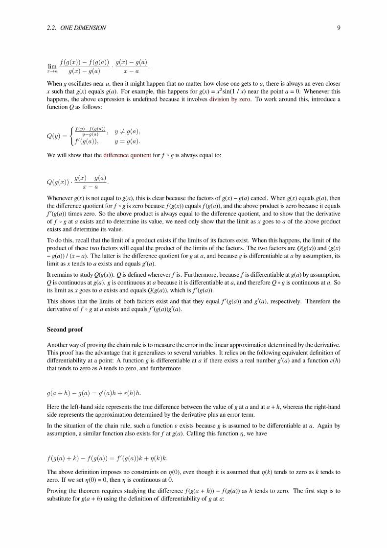
When g oscillates near a, then it might happen that no matter how close one gets to a, there is always an even closerx such that g(x) equals g(a). For example, this happens for g(x) = x2sin(1 / x) near the point a = 0. Whenever thishappens, the above expression is undefined because it involves division by zero. To work around this, introduce afunction Q as follows:
Q(y) =
f(y)−f(g(a))
y−g(a) , y = g(a),
f ′(g(a)), y = g(a).
We will show that the difference quotient for f ∘ g is always equal to:
Q(g(x)) · g(x)− g(a)
x− a.
Whenever g(x) is not equal to g(a), this is clear because the factors of g(x) − g(a) cancel. When g(x) equals g(a), thenthe difference quotient for f ∘ g is zero because f(g(x)) equals f(g(a)), and the above product is zero because it equalsf′(g(a)) times zero. So the above product is always equal to the difference quotient, and to show that the derivativeof f ∘ g at a exists and to determine its value, we need only show that the limit as x goes to a of the above productexists and determine its value.To do this, recall that the limit of a product exists if the limits of its factors exist. When this happens, the limit of theproduct of these two factors will equal the product of the limits of the factors. The two factors are Q(g(x)) and (g(x)− g(a)) / (x − a). The latter is the difference quotient for g at a, and because g is differentiable at a by assumption, itslimit as x tends to a exists and equals g′(a).It remains to studyQ(g(x)). Q is defined wherever f is. Furthermore, because f is differentiable at g(a) by assumption,Q is continuous at g(a). g is continuous at a because it is differentiable at a, and therefore Q ∘ g is continuous at a. Soits limit as x goes to a exists and equals Q(g(a)), which is f′(g(a)).This shows that the limits of both factors exist and that they equal f′(g(a)) and g′(a), respectively. Therefore thederivative of f ∘ g at a exists and equals f′(g(a))g′(a).
Second proof
Another way of proving the chain rule is to measure the error in the linear approximation determined by the derivative.This proof has the advantage that it generalizes to several variables. It relies on the following equivalent definition ofdifferentiability at a point: A function g is differentiable at a if there exists a real number g′(a) and a function ε(h)that tends to zero as h tends to zero, and furthermore
g(a+ h)− g(a) = g′(a)h+ ε(h)h.
Here the left-hand side represents the true difference between the value of g at a and at a + h, whereas the right-handside represents the approximation determined by the derivative plus an error term.In the situation of the chain rule, such a function ε exists because g is assumed to be differentiable at a. Again byassumption, a similar function also exists for f at g(a). Calling this function η, we have
f(g(a) + k)− f(g(a)) = f ′(g(a))k + η(k)k.
The above definition imposes no constraints on η(0), even though it is assumed that η(k) tends to zero as k tends tozero. If we set η(0) = 0, then η is continuous at 0.Proving the theorem requires studying the difference f(g(a + h)) − f(g(a)) as h tends to zero. The first step is tosubstitute for g(a + h) using the definition of differentiability of g at a:
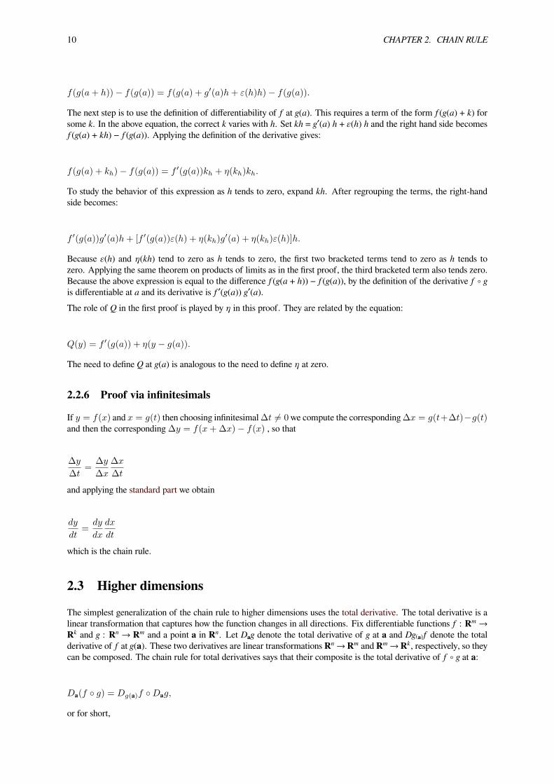
10 CHAPTER 2. CHAIN RULE
f(g(a+ h))− f(g(a)) = f(g(a) + g′(a)h+ ε(h)h)− f(g(a)).
The next step is to use the definition of differentiability of f at g(a). This requires a term of the form f(g(a) + k) forsome k. In the above equation, the correct k varies with h. Set kh = g′(a) h + ε(h) h and the right hand side becomesf(g(a) + kh) − f(g(a)). Applying the definition of the derivative gives:
f(g(a) + kh)− f(g(a)) = f ′(g(a))kh + η(kh)kh.
To study the behavior of this expression as h tends to zero, expand kh. After regrouping the terms, the right-handside becomes:
f ′(g(a))g′(a)h+ [f ′(g(a))ε(h) + η(kh)g′(a) + η(kh)ε(h)]h.
Because ε(h) and η(kh) tend to zero as h tends to zero, the first two bracketed terms tend to zero as h tends tozero. Applying the same theorem on products of limits as in the first proof, the third bracketed term also tends zero.Because the above expression is equal to the difference f(g(a + h)) − f(g(a)), by the definition of the derivative f ∘ gis differentiable at a and its derivative is f′(g(a)) g′(a).The role of Q in the first proof is played by η in this proof. They are related by the equation:
Q(y) = f ′(g(a)) + η(y − g(a)).
The need to define Q at g(a) is analogous to the need to define η at zero.
2.2.6 Proof via infinitesimals
If y = f(x) and x = g(t) then choosing infinitesimal∆t = 0we compute the corresponding∆x = g(t+∆t)−g(t)and then the corresponding∆y = f(x+∆x)− f(x) , so that
∆y
∆t=
∆y
∆x
∆x
∆t
and applying the standard part we obtain
dy
dt=dy
dx
dx
dt
which is the chain rule.
2.3 Higher dimensions
The simplest generalization of the chain rule to higher dimensions uses the total derivative. The total derivative is alinear transformation that captures how the function changes in all directions. Fix differentiable functions f : Rm →Rk and g : Rn → Rm and a point a in Rn. Let Dₐg denote the total derivative of g at a and Dg₍ₐ₎f denote the totalderivative of f at g(a). These two derivatives are linear transformations Rn → Rm and Rm → Rk, respectively, so theycan be composed. The chain rule for total derivatives says that their composite is the total derivative of f ∘ g at a:
Da(f g) = Dg(a)f Dag,
or for short,
2.3. HIGHER DIMENSIONS 11
D(f g) = Df Dg.
The higher-dimensional chain rule can be proved using a technique similar to the second proof given above.Because the total derivative is a linear transformation, the functions appearing in the formula can be rewritten asmatrices. The matrix corresponding to a total derivative is called a Jacobian matrix, and the composite of twoderivatives corresponds to the product of their Jacobian matrices. From this perspective the chain rule thereforesays:
Jfg(a) = Jf (g(a))Jg(a),
or for short,
Jfg = (Jf g)Jg.
That is, the Jacobian of the composite function is the product of the Jacobians of the composed functions (evaluatedat the appropriate points).The higher-dimensional chain rule is a generalization of the one-dimensional chain rule. If k, m, and n are 1, so thatf : R→ R and g : R→ R, then the Jacobian matrices of f and g are 1 × 1. Specifically, they are:
Jg(a) =(g′(a)
),
Jf (g(a)) =(f ′(g(a))
).
The Jacobian of f ∘ g is the product of these 1 × 1matrices, so it is f′(g(a))⋅g′(a), as expected from the one-dimensionalchain rule. In the language of linear transformations, Da(g) is the function which scales a vector by a factor of g′(a)and Dg₍a₎(f) is the function which scales a vector by a factor of f′(g(a)). The chain rule says that the composite ofthese two linear transformations is the linear transformation Da(f ∘ g), and therefore it is the function that scales avector by f′(g(a))⋅g′(a).Another way of writing the chain rule is used when f and g are expressed in terms of their components as y = f(u)= (f1(u), ..., fk(u)) and u = g(x) = (g1(x), ..., gm(x)). In this case, the above rule for Jacobian matrices is usuallywritten as:
∂(y1, . . . , yk)
∂(x1, . . . , xn)=
∂(y1, . . . , yk)
∂(u1, . . . , um)
∂(u1, . . . , um)
∂(x1, . . . , xn).
The chain rule for total derivatives implies a chain rule for partial derivatives. Recall that when the total derivativeexists, the partial derivative in the ith coordinate direction is found by multiplying the Jacobian matrix by the ith basisvector. By doing this to the formula above, we find:
∂(y1, . . . , yk)
∂xi=
∂(y1, . . . , yk)
∂(u1, . . . , um)
∂(u1, . . . , um)
∂xi.
Since the entries of the Jacobian matrix are partial derivatives, we may simplify the above formula to get:
∂(y1, . . . , yk)
∂xi=
m∑ℓ=1
∂(y1, . . . , yk)
∂uℓ
∂uℓ∂xi
.
More conceptually, this rule expresses the fact that a change in the xi direction may change all of g1 through gk, andany of these changes may affect f.In the special case where k = 1, so that f is a real-valued function, then this formula simplifies even further:
12 CHAPTER 2. CHAIN RULE
∂y
∂xi=
m∑ℓ=1
∂y
∂uℓ
∂uℓ∂xi
.
This can be rewritten as a dot product. Recalling that u = (g1, ..., gm), the partial derivative ∂u / ∂xi is also a vector,and the chain rule says that:
∂y
∂xi= ∇f · ∂u
∂xi.
2.3.1 Example
Given u(x, y) = x2 + 2y where x(r, t) = r sin(t) and y(r,t) = sin2(t), determine the value of ∂u / ∂r and ∂u / ∂t usingthe chain rule.
∂u
∂r=∂u
∂x
∂x
∂r+∂u
∂y
∂y
∂r= (2x)(sin(t)) + (2)(0) = 2r sin2(t),
and
∂u
∂t=∂u
∂x
∂x
∂t+∂u
∂y
∂y
∂t
= (2x)(r cos(t)) + (2)(2 sin(t) cos(t))= (2r sin(t))(r cos(t)) + 4 sin(t) cos(t)= 2(r2 + 2) sin(t) cos(t)= (r2 + 2) sin(2t).
2.3.2 Higher derivatives of multivariable functions
Main article: Faà di Bruno’s formula § Multivariate version
Faà di Bruno’s formula for higher-order derivatives of single-variable functions generalizes to the multivariable case.If y = f(u) is a function of u = g(x) as above, then the second derivative of f ∘ g is:
∂2y
∂xi∂xj=∑k
(∂y
∂uk
∂2uk∂xi∂xj
)+∑k,ℓ
(∂2y
∂uk∂uℓ
∂uk∂xi
∂uℓ∂xj
).
2.4 Further generalizations
All extensions of calculus have a chain rule. In most of these, the formula remains the same, though the meaning ofthat formula may be vastly different.One generalization is to manifolds. In this situation, the chain rule represents the fact that the derivative of f ∘ g isthe composite of the derivative of f and the derivative of g. This theorem is an immediate consequence of the higherdimensional chain rule given above, and it has exactly the same formula.The chain rule is also valid for Fréchet derivatives in Banach spaces. The same formula holds as before. This caseand the previous one admit a simultaneous generalization to Banach manifolds.In abstract algebra, the derivative is interpreted as a morphism of modules of Kähler differentials. A ring homomor-phism of commutative rings f : R→ S determines a morphism of Kähler differentials Df : ΩR→ΩS which sends anelement dr to d(f(r)), the exterior differential of f(r). The formula D(f ∘ g) = Df ∘ Dg holds in this context as well.

2.5. SEE ALSO 13
The common feature of these examples is that they are expressions of the idea that the derivative is part of a functor.A functor is an operation on spaces and functions between them. It associates to each space a new space and toeach function between two spaces a new function between the corresponding new spaces. In each of the above cases,the functor sends each space to its tangent bundle and it sends each function to its derivative. For example, in themanifold case, the derivative sends a Cr-manifold to a Cr−1-manifold (its tangent bundle) and a Cr-function to its totalderivative. There is one requirement for this to be a functor, namely that the derivative of a composite must be thecomposite of the derivatives. This is exactly the formula D(f ∘ g) = Df ∘ Dg.There are also chain rules in stochastic calculus. One of these, Itō's lemma, expresses the composite of an Itō process(or more generally a semimartingale) dXt with a twice-differentiable function f. In Itō's lemma, the derivative ofthe composite function depends not only on dXt and the derivative of f but also on the second derivative of f. Thedependence on the second derivative is a consequence of the non-zero quadratic variation of the stochastic process,which broadly speaking means that the process can move up and down in a very rough way. This variant of the chainrule is not an example of a functor because the two functions being composed are of different types.
2.5 See also• Integration by substitution
• Leibniz integral rule
• Quotient rule
• Triple product rule
• Product rule
• Automatic differentiation, a computational method that makes heavy use of the chain rule to compute exactnumerical derivatives.
2.6 References[1] Omar Hernández Rodríguez and Jorge M. López Fernández (2010). “A Semiotic Reflection on the Didactics of the Chain
Rule” (PDF). The Montana Mathematics Enthusiast 7 (2–3): 321–332. ISSN 1551-3440.
[2] Apostol, Tom (1974). Mathematical analysis (2nd ed.). Addison Wesley. Theorem 5.5.
2.7 External links• Hazewinkel, Michiel, ed. (2001), “Leibniz rule”, Encyclopedia of Mathematics, Springer, ISBN 978-1-55608-010-4
• Weisstein, Eric W., “Chain Rule”, MathWorld.
• Khan Academy Lesson 1 Lesson 3
• http://calculusapplets.com/chainrule.html
• The Chain Rule explained

Chapter 3
Darboux’s theorem (analysis)
Darboux’s theorem is a theorem in real analysis, named after Jean Gaston Darboux. It states that all functions thatresult from the differentiation of other functions have the intermediate value property: the image of an interval isalso an interval.When f is continuously differentiable (f in C1([a,b])), this is a consequence of the intermediate value theorem. Buteven when f′ is not continuous, Darboux’s theorem places a severe restriction on what it can be.
3.1 Darboux’s theorem
Let I be an open interval, f : I → R a real-valued differentiable function. Then f ′ has the intermediate valueproperty: If a and b are points in I with a < b , then for every y between f ′(a) and f ′(b) , there exists an x in [a, b]such that f ′(x) = y .[1]
3.2 Proof
If y equals f ′(a) or f ′(b) , then setting x equal to a or b , respectively, works. Therefore, without loss of generality,we may assume that y is strictly between f ′(a) and f ′(b) , and in particular that f ′(a) > y > f ′(b) . Define a newfunction ϕ : I → R by
ϕ(t) = f(t)− yt.
Since ϕ is continuous on the closed interval [a, b] , its maximum value on that interval is attained, according to theextreme value theorem, at a point x in that interval, i.e. at some x ∈ [a, b] . Because ϕ′(a) = f ′(a)−y > y−y = 0and ϕ′(b) = f ′(b) − y < y − y = 0 , Fermat’s theorem implies that neither a nor b can be a point, such as x ,at which ϕ attains a local maximum. Therefore, x ∈ (a, b) . Hence, again by Fermat’s theorem, ϕ′(x) = 0 , i.e.f ′(x) = y .[1]
Another proof based solely on the mean value theorem and the intermediate value theorem is due to Lars Olsen.[1]
3.3 Darboux function
A Darboux function is a real-valued function f which has the “intermediate value property": for any two values aand b in the domain of f, and any y between f(a) and f(b), there is some c between a and b with f(c) = y.[2] By theintermediate value theorem, every continuous function is a Darboux function. Darboux’s contribution was to showthat there are discontinuous Darboux functions.Every discontinuity of a Darboux function is essential, that is, at any point of discontinuity, at least one of the lefthand and right hand limits does not exist.
14

3.4. NOTES 15
An example of a Darboux function that is discontinuous at one point, is the function x 7→ sin(1/x) .By Darboux’s theorem, the derivative of any differentiable function is a Darboux function. In particular, the derivativeof the function x 7→ x2 sin(1/x) is a Darboux function that is not continuous.An example of a Darboux function that is nowhere continuous is the Conway base 13 function.Darboux functions are a quite general class of functions. It turns out that any real-valued function f on the real linecan be written as the sum of two Darboux functions.[3] This implies in particular that the class of Darboux functionsis not closed under addition.A strongly Darboux function is one for which the image of every (non-empty) open interval is the whole real line.Such functions exist and are Darboux but nowhere continuous.[2]
3.4 Notes[1] Olsen, Lars: A New Proof of Darboux’s Theorem, Vol. 111, No. 8 (Oct., 2004) (pp. 713–715), The American Mathemat-
ical Monthly
[2] Ciesielski, Krzysztof (1997). Set theory for the working mathematician. London Mathematical Society Student Texts 39.Cambridge: Cambridge University Press. pp. 106–111. ISBN 0-521-59441-3. Zbl 0938.03067.
[3] Bruckner, Andrew M: Differentiation of real functions, 2 ed, page 6, American Mathematical Society, 1994
3.5 External links• This article incorporates material from Darboux’s theorem on PlanetMath, which is licensed under the Creative
Commons Attribution/Share-Alike License.
• Hazewinkel, Michiel, ed. (2001), “Darboux theorem”, Encyclopedia of Mathematics, Springer, ISBN 978-1-55608-010-4

Chapter 4
Divergence theorem
“Gauss’s theorem” redirects here. For Gauss’s theorem concerning the electric field, see Gauss’s law.“Ostrogradsky theorem” redirects here. For Ostrogradsky’s theorem concerning the linear instability of the Hamil-tonian associated with a Lagrangian dependent on higher time derivatives than the first, see Ostrogradsky instability.
In vector calculus, the divergence theorem, also known as Gauss’s theorem or Ostrogradsky’s theorem,[1][2] is aresult that relates the flow (that is, flux) of a vector field through a surface to the behavior of the vector field insidethe surface.More precisely, the divergence theorem states that the outward flux of a vector field through a closed surface is equalto the volume integral of the divergence over the region inside the surface. Intuitively, it states that the sum of allsources minus the sum of all sinks gives the net flow out of a region.The divergence theorem is an important result for the mathematics of engineering, in particular in electrostatics andfluid dynamics.In physics and engineering, the divergence theorem is usually applied in three dimensions. However, it generalizesto any number of dimensions. In one dimension, it is equivalent to the fundamental theorem of calculus. In twodimensions, it is equivalent to Green’s theorem.The theorem is a special case of the more general Stokes’ theorem.[3]
4.1 Intuition
If a fluid is flowing in some area, then the rate at which fluid flows out of a certain region within that area can becalculated by adding up the sources inside the region and subtracting the sinks. The fluid flow is represented by avector field, and the vector field’s divergence at a given point describes the strength of the source or sink there. So,integrating the field’s divergence over the interior of the region should equal the integral of the vector field over theregion’s boundary. The divergence theorem says that this is true.[4]
The divergence theorem is employed in any conservation law which states that the volume total of all sinks andsources, that is the volume integral of the divergence, is equal to the net flow across the volume’s boundary.[5]
4.2 Mathematical statement
Suppose V is a subset of Rn (in the case of n = 3, V represents a volume in 3D space) which is compact and has apiecewise smooth boundary S (also indicated with ∂V = S ). If F is a continuously differentiable vector field definedon a neighborhood of V, then we have:[6]
∫∫∫V(∇ · F) dV = S (F · n) dS.
16
4.2. MATHEMATICAL STATEMENT 17
V
Sn
nn
n
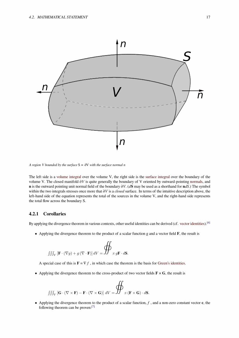
A region V bounded by the surface S = ∂V with the surface normal n
The left side is a volume integral over the volume V, the right side is the surface integral over the boundary of thevolume V. The closed manifold ∂V is quite generally the boundary of V oriented by outward-pointing normals, andn is the outward pointing unit normal field of the boundary ∂V. (dSmay be used as a shorthand for ndS.) The symbolwithin the two integrals stresses once more that ∂V is a closed surface. In terms of the intuitive description above, theleft-hand side of the equation represents the total of the sources in the volume V, and the right-hand side representsthe total flow across the boundary S.
4.2.1 Corollaries
By applying the divergence theorem in various contexts, other useful identities can be derived (cf. vector identities).[6]
• Applying the divergence theorem to the product of a scalar function g and a vector field F, the result is
∫∫∫V[F · (∇g) + g (∇ · F)] dV = S gF · dS.
A special case of this is F = ∇ f , in which case the theorem is the basis for Green’s identities.
• Applying the divergence theorem to the cross-product of two vector fields F × G, the result is
∫∫∫V[G · (∇× F)− F · (∇×G)] dV = S (F×G) · dS.
• Applying the divergence theorem to the product of a scalar function, f , and a non-zero constant vector c, thefollowing theorem can be proven:[7]

18 CHAPTER 4. DIVERGENCE THEOREM
The divergence theorem can be used to calculate a flux through a closed surface that fully encloses a volume, like any of the surfaceson the left. It can not directly be used to calculate the flux through surfaces with boundaries, like those on the right. (Surfaces areblue, boundaries are red.)
∫∫∫Vc · ∇f dV = S (cf) · dS−
∫∫∫Vf(∇ · c) dV.
• Applying the divergence theorem to the cross-product of a vector field F and a non-zero constant vector c, thefollowing theorem can be proven:[7]
∫∫∫Vc · (∇× F) dV = S (F× c) · dS.

4.3. EXAMPLE 19
4.3 Example
The vector field corresponding to the example shown. Note, vectors may point into or out of the sphere.
Suppose we wish to evaluate
S F · n dS,
where S is the unit sphere defined by
S =x, y, z ∈ R3 : x2 + y2 + z2 = 1
.
and F is the vector field
F = 2xi+ y2j+ z2k.
The direct computation of this integral is quite difficult, but we can simplify the derivation of the result using thedivergence theorem, because the divergence theorem says that the integral is equal to:

20 CHAPTER 4. DIVERGENCE THEOREM
∫∫∫W
(∇ · F) dV = 2
∫∫∫W
(1 + y + z) dV = 2
∫∫∫W
dV + 2
∫∫∫W
y dV + 2
∫∫∫W
z dV.
where W is the unit ball:
W =x, y, z ∈ R3 : x2 + y2 + z2 ≤ 1
.
Since the function y is positive in one hemisphere of W and negative in the other, in an equal and opposite way, itstotal integral over W is zero. The same is true for z:
∫∫∫W
y dV =
∫∫∫W
z dV = 0.
Therefore,
S F · n dS = 2∫∫∫
WdV = 8π
3 ,
because the unit ball W has volume 4π/3.
4.4 Applications
4.4.1 Differential form and integral form of physical laws
As a result of the divergence theorem, a host of physical laws can be written in both a differential form (where onequantity is the divergence of another) and an integral form (where the flux of one quantity through a closed surfaceis equal to another quantity). Three examples are Gauss’s law (in electrostatics), Gauss’s law for magnetism, andGauss’s law for gravity.
Continuity equations
Main article: continuity equation
Continuity equations offer more examples of laws with both differential and integral forms, related to each other bythe divergence theorem. In fluid dynamics, electromagnetism, quantum mechanics, relativity theory, and a numberof other fields, there are continuity equations that describe the conservation of mass, momentum, energy, probability,or other quantities. Generically, these equations state that the divergence of the flow of the conserved quantity isequal to the distribution of sources or sinks of that quantity. The divergence theorem states that any such continuityequation can be written in a differential form (in terms of a divergence) and an integral form (in terms of a flux).[8]
4.4.2 Inverse-square laws
Any inverse-square law can instead be written in a Gauss’ law-type form (with a differential and integral form, asdescribed above). Two examples are Gauss’ law (in electrostatics), which follows from the inverse-square Coulomb’slaw, and Gauss’ law for gravity, which follows from the inverse-square Newton’s law of universal gravitation. Thederivation of the Gauss’ law-type equation from the inverse-square formulation (or vice versa) is exactly the same inboth cases; see either of those articles for details.[8]

4.5. HISTORY 21
4.5 History
The theorem was first discovered by Lagrange in 1762,[9] then later independently rediscovered by Gauss in 1813,[10]by Ostrogradsky, who also gave the first proof of the general theorem, in 1826,[11] by Green in 1828,[12] etc.[13]Subsequently, variations on the divergence theorem are correctly called Ostrogradsky’s theorem, but also commonlyGauss’s theorem, or Green’s theorem.
4.6 Examples
To verify the planar variant of the divergence theorem for a region R:
R =x, y ∈ R2 : x2 + y2 ≤ 1
,
and the vector field:
F(x, y) = 2yi+ 5xj.
The boundary of R is the unit circle, C, that can be represented parametrically by:
x = cos(s), y = sin(s)
such that 0 ≤ s ≤ 2π where s units is the length arc from the point s = 0 to the point P on C. Then a vector equationof C is
C(s) = cos(s)i+ sin(s)j.
At a point P on C:
P = (cos(s), sin(s)) ⇒ F = 2 sin(s)i+ 5 cos(s)j.
Therefore,
∮C
F · n ds =∫ 2π
0
(2 sin(s)i+ 5 cos(s)j) · (cos(s)i+ sin(s)j) ds
=
∫ 2π
0
(2 sin(s) cos(s) + 5 sin(s) cos(s)) ds
= 7
∫ 2π
0
sin(s) cos(s) ds
= 0.
Because M = 2y, ∂M/∂x = 0, and because N = 5x, ∂N/∂y = 0. Thus
∫∫R
divF dA =
∫∫R
(∂M
∂x+∂N
∂y
)dA = 0.
4.7 Generalizations

22 CHAPTER 4. DIVERGENCE THEOREM
4.7.1 Multiple dimensions
One can use the general Stokes’ Theorem to equate the n-dimensional volume integral of the divergence of a vectorfield F over a region U to the (n − 1)-dimensional surface integral of F over the boundary of U:
∫U
∇ · F dVn =
∮∂U
F · n dSn−1
This equation is also known as the Divergence theorem.When n = 2, this is equivalent to Green’s theorem.When n = 1, it reduces to the Fundamental theorem of calculus.
4.7.2 Tensor fields
Main article: Tensor field
Writing the theorem in Einstein notation:
∫∫∫V
∂Fi
∂xidV = S Fini dS
suggestively, replacing the vector field F with a rank-n tensor field T, this can be generalized to:[14]
∫∫∫V
∂Ti1i2···iq···in∂xiq
dV = S Ti1i2···iq···inniq dS.
where on each side, tensor contraction occurs for at least one index. This form of the theorem is still in 3d, eachindex takes values 1, 2, and 3. It can be generalized further still to higher (or lower) dimensions (for example to 4dspacetime in general relativity[15]).
4.8 See also
• Stokes’ theorem
• Kelvin–Stokes theorem
4.9 Notes[1] or less correctly as Gauss' theorem (see history for reason)
[2] Katz, Victor J. (1979). “The history of Stokes’s theorem”. Mathematics Magazine (Mathematical Association of America)52: 146–156. doi:10.2307/2690275. reprinted in Anderson, Marlow (2009). Who Gave You the Epsilon?: And OtherTales of Mathematical History. Mathematical Association of America. pp. 78–79. ISBN 0883855690.
[3] Stewart, James (2008), “Vector Calculus”, Calculus: Early Transcendentals (6 ed.), Thomson Brooks/Cole, ISBN 978-0-495-01166-8
[4] R. G. Lerner, G. L. Trigg (1994). Encyclopaedia of Physics (2nd ed.). VHC. ISBN 3-527-26954-1.
[5] Byron, Frederick; Fuller, Robert (1992),Mathematics of Classical and Quantum Physics, Dover Publications, p. 22, ISBN978-0-486-67164-2

4.10. EXTERNAL LINKS 23
[6] M. R. Spiegel; S. Lipschutz; D. Spellman (2009). Vector Analysis. Schaum’s Outlines (2nd ed.). USA: McGraw Hill.ISBN 978-0-07-161545-7.
[7] MathWorld
[8] C.B. Parker (1994). McGraw Hill Encyclopaedia of Physics (2nd ed.). McGraw Hill. ISBN 0-07-051400-3.
[9] In his 1762 paper on sound, Lagrange treats a special case of the divergence theorem: Lagrange (1762) “Nouvellesrecherches sur la nature et la propagation du son” (New researches on the nature and propagation of sound), MiscellaneaTaurinensia (also known as: Mélanges de Turin ), 2: 11 - 172. This article is reprinted as: “Nouvelles recherches sur lanature et la propagation du son” in: J.A. Serret, ed., Oeuvres de Lagrange, (Paris, France: Gauthier-Villars, 1867), vol. 1,pages 151-316; on pages 263-265, Lagrange transforms triple integrals into double integrals using integration by parts.
[10] C. F. Gauss (1813) “Theoria attractionis corporum sphaeroidicorum ellipticorum homogeneorum methodo nova tractata,”Commentationes societatis regiae scientiarium Gottingensis recentiores, 2: 355-378; Gauss considered a special case of thetheorem; see the 4th, 5th, and 6th pages of his article.
[11] Mikhail Ostragradsky presented his proof of the divergence theorem to the Paris Academy in 1826; however, his work wasnot published by the Academy. He returned to St. Petersburg, Russia, where in 1828-1829 he read the work that he'd donein France, to the St. Petersburg Academy, which published his work in abbreviated form in 1831.
• His proof of the divergence theorem -- “Démonstration d'un théorème du calcul intégral” (Proof of a theorem in inte-gral calculus) -- which he had read to the Paris Academy on February 13, 1826, was translated, in 1965, into Russiantogether with another article by him. See: Юшкевич А.П. (Yushkevich A.P.) and Антропова В.И. (AntropovV.I.) (1965) "Неопубликованные работы М.В. Остроградского" (Unpublished works of MV Ostrogradskii),Историко-математические исследования (Istoriko-Matematicheskie Issledovaniya / Historical-Mathematical Stud-ies), 16: 49-96; see the section titled: "Остроградский М.В. Доказательство одной теоремы интегральногоисчисления" (Ostrogradskii M. V. Dokazatelstvo odnoy teoremy integralnogo ischislenia / OstragradskyM.V. Proofof a theorem in integral calculus).
• M. Ostrogradsky (presented: November 5, 1828 ; published: 1831) “Première note sur la théorie de la chaleur” (Firstnote on the theory of heat) Mémoires de l'Académie impériale des sciences de St. Pétersbourg, series 6, 1: 129-133;for an abbreviated version of his proof of the divergence theorem, see pages 130-131.
• Victor J. Katz (May1979) “The history of Stokes’ theorem,”Mathematics Magazine, 52(3): 146-156; for Ostragrad-sky’s proof of the divergence theorem, see pages 147-148.
[12] George Green, An Essay on the Application of Mathematical Analysis to the Theories of Electricity and Magnetism (Not-tingham, England: T. Wheelhouse, 1838). A form of the “divergence theorem” appears on pages 10-12.
[13] Other early investigators who used some form of the divergence theorem include:
• Poisson (presented: February 2, 1824 ; published: 1826) “Mémoire sur la théorie du magnétisme” (Memoir on thetheory of magnetism), Mémoires de l'Académie des sciences de l'Institut de France, 5: 247-338; on pages 294-296,Poisson transforms a volume integral (which is used to evaluate a quantity Q) into a surface integral. To make thistransformation, Poisson follows the same procedure that is used to prove the divergence theorem.
• Frédéric Sarrus (1828) “Mémoire sur les oscillations des corps flottans” (Memoir on the oscillations of floatingbodies), Annales de mathématiques pures et appliquées (Nismes), 19: 185-211.
[14] K.F. Riley, M.P. Hobson, S.J. Bence (2010). Mathematical methods for physics and engineering. Cambridge UniversityPress. ISBN 978-0-521-86153-3.
[15] see for example:J.A.Wheeler, C. Misner, K.S. Thorne (1973). Gravitation. W.H. Freeman & Co. pp. 85–86, §3.5. ISBN 0-7167-0344-0.,andR. Penrose (2007). The Road to Reality. Vintage books. ISBN 0-679-77631-1.
4.10 External links• Hazewinkel, Michiel, ed. (2001), “Ostrogradski formula”, Encyclopedia of Mathematics, Springer, ISBN 978-1-55608-010-4
• Differential Operators and the Divergence Theorem at MathPages• The Divergence (Gauss) Theorem by Nick Bykov, Wolfram Demonstrations Project.• Weisstein, Eric W., “Divergence Theorem”, MathWorld. — This article was originally based on the GFDL
article from PlanetMath at http://planetmath.org/encyclopedia/Divergence.html

Chapter 5
Extreme value theorem
This article is about continuous functions in analysis. For statistical theorems about the largest observation in asequence of random variables, see extreme value theory.In calculus, the extreme value theorem states that if a real-valued function f is continuous in the closed and bounded
a c d b
f(d)
f(c)
A continuous function ƒ(x) on the closed interval [a,b] showing the absolute max (red) and the absolute min (blue).
24

5.1. HISTORY 25
interval [a,b], then f must attain a maximum and a minimum, each at least once. That is, there exist numbers c andd in [a,b] such that:
f(c) ≥ f(x) ≥ f(d) all forx ∈ [a, b].
A related theorem is the boundedness theorem which states that a continuous function f in the closed interval [a,b]is bounded on that interval. That is, there exist real numbers m and M such that:
m ≤ f(x) ≤M all forx ∈ [a, b].
The extreme value theorem enriches the boundedness theorem by saying that not only is the function bounded, but italso attains its least upper bound as its maximum and its greatest lower bound as its minimum.The extreme value theorem is used to prove Rolle’s theorem. In a formulation due to Karl Weierstrass, this theoremstates that a continuous function from a non-empty compact space to a subset of the real numbers attains a maximumand a minimum.
5.1 History
The extreme value theorem was originally proven by Bernard Bolzano in the 1830s in a work Function Theory but thework remained unpublished until 1930. Bolzano’s proof consisted of showing that a continuous function on a closedinterval was bounded, and then showing that the function attained a maximum and a minimum value. Both proofsinvolved what is known today as the Bolzano–Weierstrass theorem (Rusnock & Kerr-Lawson 2005). The result wasalso discovered later by Weierstrass in 1860.
5.2 Functions to which the theorem does not apply
The following examples show why the function domain must be closed and bounded in order for the theorem to apply.Each fails to attain a maximum on the given interval.
1. ƒ(x) = x defined over [0, ∞) is not bounded from above.
2. ƒ(x) = x / (1 + x) defined over [0, ∞) is bounded but does not attain its least upper bound 1.
3. ƒ(x) = 1 / x defined over (0, 1] is not bounded from above.
4. ƒ(x) = 1 – x defined over (0, 1] is bounded but never attains its least upper bound 1.
Defining ƒ(0) = 0 in the last two examples shows that both theorems require continuity on [a, b].
5.3 Generalization to arbitrary topological spaces
When moving from the real line to arbitrary topological spaces, the parallel of a closed bounded interval is a compactspace.It is known that compactness is preserved by continuous functions, i.e. the image of the compact space under acontinuous mapping is also compact. A subset of the real line is compact if and only if it is both closed and bounded.This implies the following generalization of the extreme value theorem: a continuous real-valued function on anonempty compact space is bounded above and attains its supremum. Slightly more generally, this is true for anupper semicontinuous function. (see compact space#Functions and compact spaces).

26 CHAPTER 5. EXTREME VALUE THEOREM
5.4 Proving the theorems
We look at the proof for the upper bound and the maximum of f. By applying these results to the function –f, theexistence of the lower bound and the result for the minimum of f follows. Also note that everything in the proof isdone within the context of the real numbers.We first prove the boundedness theorem, which is a step in the proof of the extreme value theorem. The basic stepsinvolved in the proof of the extreme value theorem are:
1. Prove the boundedness theorem.
2. Find a sequence so that its image converges to the supremum of f.
3. Show that there exists a subsequence that converges to a point in the domain.
4. Use continuity to show that the image of the subsequence converges to the supremum.
5.4.1 Proof of the boundedness theorem
Suppose the function f is not bounded above on the interval [a,b]. Then, for every natural number n, there exists anxn in [a,b] such that f(xn) > n. This defines a sequence xn. Because [a,b] is bounded, the Bolzano–Weierstrasstheorem implies that there exists a convergent subsequence xnk
of xn. Denote its limit by x. As [a,b] isclosed, it contains x. Because f is continuous at x, we know that f( xnk
) converges to the real number f(x) (asf is sequentially continuous at x.) But f(xnk) > nk ≥ k for every k, which implies that f(xnk) diverges to +∞, acontradiction. Therefore, f is bounded above on [a,b]. ∎
5.4.2 Proof of the extreme value theorem
By the boundedness theorem, f is bounded from above, hence, by the Dedekind-completeness of the real numbers,the least upper bound (supremum) M of f exists. It is necessary to find a d in [a,b] such that M = f(d). Let n be anatural number. As M is the least upper bound, M – 1/n is not an upper bound for f. Therefore, there exists dn in[a,b] so that M – 1/n < f(dn). This defines a sequence dn. Since M is an upper bound for f, we have M – 1/n <f(dn) ≤ M for all n. Therefore, the sequence f(dn) converges to M.The Bolzano–Weierstrass theorem tells us that there exists a subsequence dnk
, which converges to some d and,as [a,b] is closed, d is in [a,b]. Since f is continuous at d, the sequence f( dnk
) converges to f(d). But f(dnk)is a subsequence of f(dn) that converges to M, so M = f(d). Therefore, f attains its supremum M at d. ∎
5.4.3 Alternative proof of the extreme value theorem
The set y ∈ R : y = f(x) for some x ∈ [a,b] is a bounded set. Hence, its least upper bound exists by least upperbound property of the real numbers. Let M = sup(f(x)) on [a, b]. If there is no point x on [a, b] so that f(x) = Mthen f(x) < M on [a, b]. Therefore 1/(M − f(x)) is continuous on [a, b].However, to every positive number ε, there is always some x in [a, b] such that M − f(x) < ε because M is the leastupper bound. Hence, 1/(M − f(x)) > 1/ε, which means that 1/(M − f(x)) is not bounded. Since every continuousfunction on a [a, b] is bounded, this contradicts the conclusion that 1/(M − f(x)) was continuous on [a, b]. Thereforethere must be a point x in [a, b] such that f(x) = M. ∎
5.4.4 Proof using the hyperreals
In the setting of non-standard calculus, let N be an infinite hyperinteger. The interval [0, 1] has a natural hyperrealextension. Consider its partition into N subintervals of equal infinitesimal length 1/N, with partition points xi = i /Nas i “runs” from 0 to N. The function ƒ is also naturally extended to a function ƒ* defined on the hyperreals between 0and 1. Note that in the standard setting (when N is finite), a point with the maximal value of ƒ can always be chosenamong the N+1 points xi, by induction. Hence, by the transfer principle, there is a hyperinteger i0 such that 0 ≤ i0 ≤N and f∗(xi0) ≥ f∗(xi) for all i = 0, …, N. Consider the real point
5.5. EXTENSION TO SEMI-CONTINUOUS FUNCTIONS 27
c = st(xi0)
where st is the standard part function. An arbitrary real point x lies in a suitable sub-interval of the partition, namelyx ∈ [xi, xi+1] , so that st(xi) = x. Applying st to the inequality f∗(xi0) ≥ f∗(xi) , we obtain st(f∗(xi0)) ≥st(f∗(xi)) . By continuity of ƒ we have
st(f∗(xi0)) = f(st(xi0)) = f(c)
Hence ƒ(c) ≥ ƒ(x), for all real x, proving c to be a maximum of ƒ. See Keisler (1986, p. 164).
5.5 Extension to semi-continuous functions
If the continuity of the function f is weakened to semi-continuity, then the corresponding half of the boundednesstheorem and the extreme value theorem hold and the values –∞ or +∞, respectively, from the extended real numberline can be allowed as possible values. More precisely:Theorem: If a function f : [a,b] → [–∞,∞) is upper semi-continuous, meaning that
lim supy→x
f(y) ≤ f(x)
for all x in [a,b], then f is bounded above and attains its supremum.Proof: If f(x) = –∞ for all x in [a,b], then the supremum is also –∞ and the theorem is true. In all other cases,the proof is a slight modification of the proofs given above. In the proof of the boundedness theorem, the uppersemi-continuity of f at x only implies that the limit superior of the subsequence f(xnk) is bounded above by f(x) <∞, but that is enough to obtain the contradiction. In the proof of the extreme value theorem, upper semi-continuityof f at d implies that the limit superior of the subsequence f(dnk) is bounded above by f(d), but this suffices toconclude that f(d) = M. ∎Applying this result to −f proves:Theorem: If a function f : [a,b] → (–∞,∞] is lower semi-continuous, meaning that
lim infy→x
f(y) ≥ f(x)
for all x in [a,b], then f is bounded below and attains its infimum.A real-valued function is upper as well as lower semi-continuous, if and only if it is continuous in the usual sense.Hence these two theorems imply the boundedness theorem and the extreme value theorem.
5.6 References• Keisler, H. Jerome (1986). Elementary calculus. An infinitesimal approach. Boston, Massachusetts: Prindle,Weber & Schmidt. ISBN 0-87150-911-3.
5.7 External links• A Proof for extreme value theorem at cut-the-knot
• Boundedness Theorem at PlanetMath.org.
• Extreme Value Theorem at PlanetMath.org.

28 CHAPTER 5. EXTREME VALUE THEOREM
• Extreme Value Theorem by Jacqueline Wandzura with additional contributions by Stephen Wandzura, theWolfram Demonstrations Project.
• Weisstein, Eric W., “Extreme Value Theorem”, MathWorld.

Chapter 6
Fermat’s theorem (stationary points)
This article is about Fermat’s theorem concerning the maximums and minimums of functions. For other theoremsalso named after Pierre de Fermat, see Fermat’s theorem.
In mathematics, Fermat’s theorem (also known as Interior extremum theorem) is a method to find local maximaand minima of differentiable functions on open sets by showing that every local extremum of the function is astationary point (the function derivative is zero in that point). Fermat’s theorem is a theorem in real analysis, namedafter Pierre de Fermat.By using Fermat’s theorem, the potential extrema of a function f , with derivative f ′ , are found by solving an equationin f ′ . Fermat’s theorem gives only a necessary condition for extreme function values, and some stationary points areinflection points (not a maximum or minimum). The function’s second derivative, if it exists, can determine if anystationary point is a maximum, minimum, or inflection point.
6.1 Statement
One way to state Fermat’s theorem is that whenever you compute the derivative of a function’s local extrema, theresult will always be zero. In precise mathematical language:
Let f : (a, b) → R be a function and suppose that x0 ∈ (a, b) is a local extremum of f . If f isdifferentiable at x0 , then f ′(x0) = 0 .
Another way to understand the theorem is via the contrapositive statement. If the derivative of a function at any pointis not zero, that point is not an extrema. Formally:
If f is differentiable at x0 ∈ (a, b) , and f ′(x0) = 0 , then x0 is not a local extremum of f.
6.1.1 Corollary
The global extrema of a function f on a domain A occur only at boundaries, non-differentiable points, and stationarypoints. If x0 is a global extremum of f, then one of the following is true:
• boundary: x0 is in the boundary of A• non-differentiable: f is not differentiable at x0• stationary point: x0 is a stationary point of f
6.1.2 Extension
In higher dimensions, exactly the same statement holds; however, the proof is slightly more complicated. The com-plication is that in 1 dimension, one can either move left or right from a point, while in higher dimensions, one can
29

30 CHAPTER 6. FERMAT’S THEOREM (STATIONARY POINTS)
move in many directions. Thus, if the derivative does not vanish, one must argue that there is some direction in whichthe function increases – and thus in the opposite direction the function decreases. This is the only change to the proofor the analysis.
6.2 Applications
See also: maxima and minima
Fermat’s theorem is central to the calculusmethod of determiningmaxima andminima: in one dimension, one can findextrema by simply computing the stationary points (by computing the zeros of the derivative), the non-differentiablepoints, and the boundary points, and then investigating this set to determine the extrema.One can do this either by evaluating the function at each point and taking themaximum, or by analyzing the derivativesfurther, using the first derivative test, the second derivative test, or the higher-order derivative test.
6.3 Intuitive argument
Intuitively, a differentiable function is approximated by its derivative – a differentiable function behaves infinitesimallylike a linear function a+ bx, or more precisely, f(x0) + f ′(x0) · (x− x0). Thus, from the perspective that “if f isdifferentiable and has non-vanishing derivative at x0, then it does not attain an extremum at x0, " the intuition is thatif the derivative at x0 is positive, the function is increasing near x0, while if the derivative is negative, the function isdecreasing near x0. In both cases, it cannot attain a maximum or minimum, because its value is changing. It can onlyattain a maximum or minimum if it “stops” – if the derivative vanishes (or if it is not differentiable, or if one runsinto the boundary and cannot continue). However, making “behaves like a linear function” precise requires carefulanalytic proof.More precisely, the intuition can be stated as: if the derivative is positive, there is some point to the right of x0 wheref is greater, and some point to the left of x0 where f is less, and thus f attains neither a maximum nor a minimum atx0. Conversely, if the derivative is negative, there is a point to the right which is lesser, and a point to the left whichis greater. Stated this way, the proof is just translating this into equations and verifying “how much greater or less”.The intuition is based on the behavior of polynomial functions. Assume that function f has a maximum at x0,the reasoning being similar for a function minimum. If x0 ∈ (a, b) is a local maximum then, roughly, there is a(possibly small) neighborhood of x0 such as the function “is increasing before” and “decreasing after”[note 1] x0 . Asthe derivative is positive for an increasing function and negative for a decreasing function, f ′ is positive before andnegative after x0 . f ′ doesn't skip values (by Darboux’s theorem), so it has to be zero at some point between thepositive and negative values. The only point in the neighbourhood where it is possible to have f ′(x) = 0 is x0 .The theorem (and its proof below) is more general than the intuition in that it doesn't require the function to bedifferentiable over a neighbourhood around x0 . It is sufficient for the function to be differentiable only in the extremepoint.
6.4 Proof
6.4.1 Proof 1: Non-vanishing derivatives implies not extremum
Suppose that f is differentiable at x0 ∈ (a, b), with derivative K, and assume without loss of generality that K > 0,so the tangent line at x0 has positive slope (is increasing). Then there is a neighborhood of x0 on which the secantlines through x0 all have positive slope, and thus to the right of x0, f is greater, and to the left of x0, f is lesser.The schematic of the proof is:
• an infinitesimal statement about derivative (tangent line) at x0 implies
• a local statement about difference quotients (secant lines) near x0, which implies
• a local statement about the value of f near x0.
6.5. CAUTIONS 31
Formally, by the definition of derivative, f ′(x0) = K means that
limϵ→0
f(x0 + ϵ)− f(x0)
ϵ= K.
In particular, for sufficiently small ϵ (less than some ϵ0 ), the fraction must be at leastK/2, by the definition of limit.Thus on the interval (x0 − ϵ0, x0 + ϵ0) one has:
f(x0 + ϵ)− f(x0)
ϵ> K/2;
one has replaced the equality in the limit (an infinitesimal statement) with an inequality on a neighborhood (a localstatement). Thus, rearranging the equation, if ϵ > 0, then:
f(x0 + ϵ) > f(x0) + (K/2)ϵ > f(x0),
so on the interval to the right, f is greater than f(x0), and if ϵ < 0, then:
f(x0 + ϵ) < f(x0) + (K/2)ϵ < f(x0),
so on the interval to the left, f is less than f(x0).Thus x0 is not a local or global maximum or minimum of f.
6.4.2 Proof 2: Extremum implies derivative vanishes
Alternatively, one can start by assuming that x0 is a local maximum, and then prove that the derivative is 0.Suppose that x0 is a local maximum (a similar proof applies if x0 is a local minimum). Then there ∃ δ > 0 such that(x0 − δ, x0 + δ) ⊂ (a, b) and such that we have f(x0) ≥ f(x) ∀x with |x− x0| < δ . Hence for any h ∈ (0, δ) wenotice that it holds
f(x0 + h)− f(x0)
h≤ 0.
Since the limit of this ratio as h gets close to 0 from above exists and is equal to f ′(x0) we conclude that f ′(x0) ≤ 0. On the other hand for h ∈ (−δ, 0) we notice that
f(x0 + h)− f(x0)
h≥ 0
but again the limit as h gets close to 0 from below exists and is equal to f ′(x0) so we also have f ′(x0) ≥ 0 .Hence we conclude that f ′(x0) = 0.
6.5 Cautions
A subtle misconception that is often held in the context of Fermat’s theorem is to assume that it makes a strongerstatement about local behavior than it does. Notably, Fermat’s theorem does not say that functions (monotonically)“increase up to” or “decrease down from” a local maximum. This is very similar to the misconception that a limitmeans “monotonically getting closer to a point”. For “well-behaved functions” (which here mean continuously dif-ferentiable), some intuitions hold, but in general functions may be ill-behaved, as illustrated below. The moral is thatderivatives determine infinitesimal behavior, and that continuous derivatives determine local behavior.

32 CHAPTER 6. FERMAT’S THEOREM (STATIONARY POINTS)
6.5.1 Continuously differentiable functions
If f is continuously differentiable ( C1 ) on a neighborhood of x0, then f ′(x0) > 0 does mean that f is increasing ona neighborhood of x0, as follows.If f ′(x0) = K > 0 and f ∈ C1, then by continuity of the derivative, there is a neighborhood (x0 − ϵ0, x0 + ϵ0)of x0 on which f ′(x0) > K/2. Then f is increasing on this interval, by the mean value theorem: the slope of anysecant line is at leastK/2, as it equals the slope of some tangent line.However, in the general statement of Fermat’s theorem, where one is only given that the derivative at x0 is positive,one can only conclude that secant lines through x0 will have positive slope, for secant lines between x0 and nearenough points.Conversely, if the derivative of f at a point is zero ( x0 is a stationary point), one cannot in general conclude anythingabout the local behavior of f – it may increase to one side and decrease to the other (as in x3 ), increase to bothsides (as in x4 ), decrease to both sides (as in −x4 ), or behave in more complicated ways, such as oscillating (as inx2(sin(1/x)) , as discussed below).One can analyze the infinitesimal behavior via the second derivative test and higher-order derivative test, if the functionis differentiable enough, and if the first non-vanishing derivative at x0 is a continuous function, one can then concludelocal behavior (i.e., if f (k)(x0) = 0 is the first non-vanishing derivative, and f (k) is continuous, so f ∈ Ck ), thenone can treat f as locally close to a polynomial of degree k, since it behaves approximately as f (k)(x0)(x−x0)k, butif the kth derivative is not continuous, one cannot draw such conclusions, and it may behave rather differently.
6.5.2 Pathological functions
Consider the function sin(1/x) – it oscillates increasingly rapidly between−1 and 1 as x approaches 0. Consider thenf(x) = (1 + sin(1/x))x2 – this oscillates increasingly rapidly between 0 and 2x2 as x approaches 0. If one extendsthis function by f(0) := 0, then the function is continuous and everywhere differentiable (it is differentiable at 0 withderivative 0), but has rather unexpected behavior near 0: in any neighborhood of 0 it attains 0 infinitely many times,but also equals 2x2 (a positive number) infinitely often.Continuing in this vein, f(x) = (2 + sin(1/x))x2 oscillates between x2 and 3x2, and x = 0 is a local and globalminimum, but on no neighborhood of 0 is it decreasing down to or increasing up from 0 – it oscillates wildly near 0.This pathology can be understood because, while the function is everywhere differentiable, it is not continuouslydifferentiable: the limit of f ′(x) as x → 0 does not exist, so the derivative is not continuous at 0. This reflects theoscillation between increasing and decreasing values as it approaches 0.
6.6 See also
• Optimization (mathematics)
• Maxima and minima
• Derivative
• Extreme value
• arg max
• Adequality
6.7 Notes
[1] This intuition is only correct for continuously differentiable ( C1 ) functions, while in general it is not literally correct – afunction need not be increasing up to a local maximum: it may instead be oscillating, so neither increasing nor decreasing,but simply the local maximum is greater than any values in a small neighborhood to the left or right of it. See details in thepathologies.

6.8. EXTERNAL LINKS 33
6.8 External links• Fermat’s Theorem (stationary points) at PlanetMath.org.
• Proof of Fermat’s Theorem (stationary points) at PlanetMath.org.

Chapter 7
Fubini’s theorem
For the Fubini theorem for category, see Kuratowski–Ulam theorem.
In mathematical analysis Fubini’s theorem, introduced by Guido Fubini (1907), is a result which gives conditionsunder which it is possible to compute a double integral using iterated integrals. Onemay switch the order of integrationif the double integral yields a finite answer when the integrand is replaced by its absolute value.
∫X
(∫Y
f(x, y) dy)dx =
∫Y
(∫X
f(x, y) dx)dy =
∫X×Y
f(x, y) d(x, y)
As a consequence it allows the order of integration to be changed in iterated integrals. Fubini’s theorem implies thatthe two repeated integrals of a function of two variables are equal if the function is integrable. Tonelli’s theoremintroduced by Leonida Tonelli (1909) is similar but applies to functions that are non-negative rather than integrable.
7.1 History
The special case of Fubini’s theorem for continuous functions on a product of closed bounded subsets of real vectorspaces was known to Euler in the 18th century. Lebesgue (1904) extended this to bounded measurable functions ona product of intervals. Levi (1906) conjectured that the theorem could be extended to functions that were integrablerather than bounded, and this was proved by Fubini (1907). Tonelli (1909) gave a variation of Fubini’s theorem thatapplies to non-negative functions rather than integrable functions.
7.2 Product measures
If X and Y are measure spaces with measures, there are several natural ways to define a product measure on theirproduct.The productX×Y ofmeasure spaces (in the sense of category theory) has as its measurable sets the σ-algebra generatedby the products A×B of measurable subsets of X and Y.A measure μ on X×Y is called a product measure if μ(A×B)=μ(A)μ(B) for measurable subsets A and B. In generalthere may be many different product measures on X×Y. Fubini’s theorem and Tonelli’s theorem both need technicalconditions to avoid this complication; the most common way is to assume all measure spaces are σ-finite, in whichcase there is a unique product measure on X×Y. There is always a unique maximal product measure on X×Y, wherethe measure of a measurable set is the inf of the measures of sets containing it that are countable unions of productsof measurable sets. The maximal product measure can be constructed by applying Carathéodory’s extension theoremto the additive function μ such that μ(A×B)=μ(A)μ(B) on the ring of sets generated by products of measurable sets.(Carathéodory’s extension theorem gives a measure on a measure space that in general contains more measurable setsthan the measure space X×Y, so strictly speaking the measure should be restricted to the σ-algebra generated by theproducts A×B of measurable subsets of X and Y.)
34

7.3. FUBINI’S THEOREM FOR INTEGRABLE FUNCTIONS 35
The product of two complete measure spaces is not usually complete. For example, the product of the Lebesguemeasure on the unit interval I with itself is not the Lebesgue measure on the square I×I. There is a variation of Fubini’stheorem for complete measures, which uses the completion of the product of measures rather than the uncompletedproduct.
7.3 Fubini’s theorem for integrable functions
Suppose X and Y are σ-finite measure spaces, and suppose that X × Y is given the product measure (which is uniqueas X and Y are σ-finite). Fubini’s theorem states that if f(x,y) is X × Y integrable, meaning that it is measurable and
∫X×Y
|f(x, y)| d(x, y) <∞,
then
∫X
(∫Y
f(x, y) dy)dx =
∫Y
(∫X
f(x, y) dx)dy =
∫X×Y
f(x, y) d(x, y).
The first two integrals are iterated integrals with respect to two measures, respectively, and the third is an integral withrespect to the product measure. The partial integrals
∫Yf(x, y) dy,
∫Xf(x, y) dx need not be defined everywhere,
but this does not matter as the points where they are not defined form a set of measure 0.If the above integral of the absolute value is not finite, then the two iterated integrals may have different values. Seebelow for an illustration of this possibility.The condition that X and Y are σ-finite is usually harmless because in practice almost all measure spaces one wishesto use Fubini’s theorem for are σ-finite. Fubini’s theorem has some rather technical extensions to the case when Xand Y are not assumed to be σ-finite (Fremlin 2003). The main extra complication in this case is that there may bemore than one product measure on X×Y. Fubini’s theorem continues to hold for the maximal product measure, butcan fail for other product measures. For example, there is a product measure and a non-negative measurable functionf for which the double integral of |f | is zero but the two iterated integrals have different values; see the section oncounterexamples below for an example of this. Tonelli’s theorem and the Fubini–Tonelli theorem (stated below) canfail on non σ-finite spaces even for the maximal product measure.
7.4 Tonelli’s theorem for non-negative functions
Tonelli’s theorem (named after Leonida Tonelli) is a successor of Fubini’s theorem. The conclusion of Tonelli’stheorem is identical to that of Fubini’s theorem, but the assumption that |f | has a finite integral is replaced by theassumption that f is non-negative.Tonelli’s theorem states that if (X, A, μ) and (Y, B, ν) are σ-finite measure spaces, while f from X×Y to [0,∞] isnon-negative and measurable, then
∫X
(∫Y
f(x, y) dy)dx =
∫Y
(∫X
f(x, y) dx)dy =
∫X×Y
f(x, y) d(x, y).
A special case of Tonelli’s theorem is in the interchange of the summations, as in∑
x
∑y axy =
∑y
∑x axy , where
axy are non-negative for all x and y. The crux of the theorem is that the interchange of order of summation holdseven if the series diverges. In effect, the only way a change in order of summation can change the sum is when thereexist some subsequences which diverge to +∞ and others diverging to −∞ . With all elements non-negative, thisdoes not happen in the stated example.Without the condition that the measure spaces are σ-finite it is possible for all three of these integrals to have differentvalues. Some authors give generalizations of Tonelli’s theorem to some measure spaces that are not σ-finite but thesegeneralizations often add conditions that immediately reduce the problem to the σ-finite case. For example, one could

36 CHAPTER 7. FUBINI’S THEOREM
take the σ-algebra onA×B to be that generated by the product of subsets of finitemeasure, rather than that generated byall products of measurable subsets,though this has the undesirable consequence that the projections from the productto its factors A and B are not measurable. Another way is to add the condition that the support of f is contained ina countable union of products of sets of finite measure. Fremlin (2003) gives some rather technical extensions ofTonelli’s theorem to some non σ-finite spaces. None of these generalizations have found any significant applicationsoutside abstract measure theory, largely because almost all measure spaces of practical interest are σ-finite.
7.5 The Fubini–Tonelli theorem
Combining Fubini’s theorem with Tonelli’s theorem gives the Fubini–Tonelli theorem (often just called Fubini’stheorem) which states that if X and Y are σ-finite measure spaces, and if f is a measurable function such that any oneof the three integrals
∫X
(∫Y
|f(x, y)| dy)dx
∫Y
(∫X
|f(x, y)| dx)dy∫
X×Y
|f(x, y)| d(x, y)
is finite then
∫X
(∫Y
f(x, y) dy)dx =
∫Y
(∫X
f(x, y) dx)dy =
∫X×Y
f(x, y) d(x, y).
The absolute value of f in the conditions above can be replaced by either the positive or the negative part of f; theseforms include Tonelli’s theorem as a special case as the negative part of a non-negative function is zero and so hasfinite integral. Informally all these conditions say that the double integral of f is well defined, though possibly infinite.The advantage of the Fubini–Tonelli over Fubini’s theorem is that the repeated integrals of the absolute value of |f |may be easier to study than the double integral. As in Fubini’s theorem, the single integrals may fail to be defined ona measure 0 set.
7.6 Fubini’s theorem for complete measures
The versions of Fubini’s and Tonelli’s theorems above have the embarrassing problem that they do not even apply tointegration on the product of the real lineRwith itself with Lebesgue measure. The problem is that Lebesgue measureon R×R is not the product of Lebesgue measure on R with itself, but rather the completion of this: a product of twocomplete measure spaces X and Y is not in general complete. For this reason one sometimes uses versions of Fubini’stheorem for complete measures: roughly speaking one just replaces all measures by their completions. The variousversions of Fubini’s theorem are similar to the versions above, with the following minor differences:
• Instead of taking a product X×Y of two measure spaces, one takes the completion of some product.
• If f is a measurable on the completion of X×Y then its restrictions to vertical or horizontal lines may be non-measurable for ameasure zero subset of lines, so one has to allow for the possibility that the vertical or horizontalintegrals are undefined on a set of measure 0 because they involve integrating non-measurable functions. Thismakes little difference, because they can already be undefined due to the functions not being integrable.
• One generally also assumes that the measures on X and Y are complete, otherwise the two partial integralsalong vertical or horizontal lines may be well-defined but not measurable. For example, if f is the characteristicfunction of a product of a measurable set and a non-measurable set contained in a measure 0 set then its singleintegral is well defined everywhere but non-measurable.

7.7. PROOFS 37
7.7 Proofs
Proofs of the Fubini and Tonelli theorems are necessarily somewhat technical, as they have to use a hypothesis relatedto σ-finiteness. Most proofs involve building up to the full theorems by proving them for increasingly complicatedfunctions as follows.
• Step 1. Use the fact that the measure on the product is a product measure to prove the theorems for thecharacteristic functions of rectangles.
• Step 2. Use the condition that the spaces are σ-finite (or some related condition) to prove the theorem for thecharacteristic functions of measurable sets. This also covers the case of simple measurable functions (measur-able functions taking only a finite number of values).
• Step 3. Use the condition that the functions are measurable to prove the theorems for positive measurablefunctions by approximating them by simple measurable functions. This proves Tonelli’s theorem.
• Step 4. Use the condition that the functions are integrable to write them as the difference of two positiveintegrable functions, and apply Tonelli’s theorem to each of these. This proves Fubini’s theorem.
7.8 Counterexamples
The following examples show how Fubini’s theorem and Tonelli’s theorem can fail if any of their hypotheses areomitted.
7.8.1 Failure of Tonelli’s theorem for non σ-finite spaces
Suppose thatX is the unit interval with the Lebesgue measurable sets and Lebesgue measure, and Y is the unit intervalwith all subsets measurable and the counting measure, so that Y is not σ-finite. If f is the characteristic function ofthe diagonal of X×Y, then integrating f along X gives the 0 function on Y, but integrating f along Y gives the function1 on X. So the two iterated integrals are different. This shows that Tonelli’s theorem can fail for spaces that are notσ-finite no matter what product measure is chosen. The measures are both decomposable, showing that Tonelli’stheorem fails for decomposable measures (which are slightly more general than σ-finite measures).
7.8.2 Failure of Fubini’s theorem for non-maximal product measures
Fubini’s theorem holds for spaces even if they are not assumed to be σ-finite provided one uses the maximal productmeasure. In the example above, for the maximal product measure, the diagonal has infinite measure so the doubleintegral of |f | is infinite, and Fubini’s theorem holds vacuously. However, if we give X×Y the product measure suchthat the measure of a set is the sum of the Lebesgue measures of its horizontal sections, then the double integral of|f | is zero, but the two iterated integrals still have different values. This gives an example of a product measure whereFubini’s theorem fails.This gives an example of two different product measures on the same product of two measure spaces. For productsof two σ-finite measure spaces, there is only one product measure.
7.8.3 Failure of Tonelli’s theorem for non-measurable functions
Suppose that X is the first uncountable ordinal, with the finite measure where the measurable sets are either countable(with measure 0) or the sets of countable complement (with measure 1). The (non-measurable) subset E of X×Xgiven by pairs (x,y) with x<y is countable on every horizontal line and has countable complement on every verticalline. If f is the characteristic function of E then the two iterated integrals of f are defined and have different values1 and 0. The function f is not measurable. This shows that Tonelli’s theorem can fail for non-measurable functions.
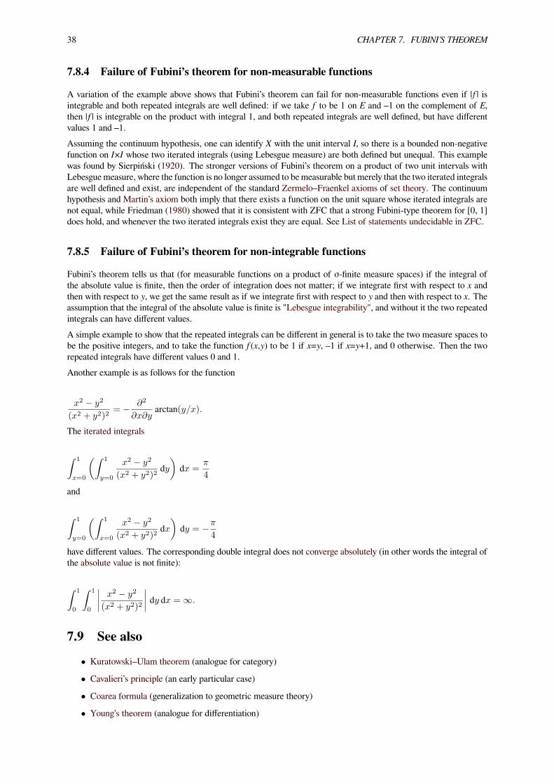
38 CHAPTER 7. FUBINI’S THEOREM
7.8.4 Failure of Fubini’s theorem for non-measurable functions
A variation of the example above shows that Fubini’s theorem can fail for non-measurable functions even if |f | isintegrable and both repeated integrals are well defined: if we take f to be 1 on E and –1 on the complement of E,then |f | is integrable on the product with integral 1, and both repeated integrals are well defined, but have differentvalues 1 and –1.Assuming the continuum hypothesis, one can identify X with the unit interval I, so there is a bounded non-negativefunction on I×I whose two iterated integrals (using Lebesgue measure) are both defined but unequal. This examplewas found by Sierpiński (1920). The stronger versions of Fubini’s theorem on a product of two unit intervals withLebesguemeasure, where the function is no longer assumed to bemeasurable but merely that the two iterated integralsare well defined and exist, are independent of the standard Zermelo–Fraenkel axioms of set theory. The continuumhypothesis and Martin’s axiom both imply that there exists a function on the unit square whose iterated integrals arenot equal, while Friedman (1980) showed that it is consistent with ZFC that a strong Fubini-type theorem for [0, 1]does hold, and whenever the two iterated integrals exist they are equal. See List of statements undecidable in ZFC.
7.8.5 Failure of Fubini’s theorem for non-integrable functions
Fubini’s theorem tells us that (for measurable functions on a product of σ-finite measure spaces) if the integral ofthe absolute value is finite, then the order of integration does not matter; if we integrate first with respect to x andthen with respect to y, we get the same result as if we integrate first with respect to y and then with respect to x. Theassumption that the integral of the absolute value is finite is "Lebesgue integrability", and without it the two repeatedintegrals can have different values.A simple example to show that the repeated integrals can be different in general is to take the two measure spaces tobe the positive integers, and to take the function f(x,y) to be 1 if x=y, –1 if x=y+1, and 0 otherwise. Then the tworepeated integrals have different values 0 and 1.Another example is as follows for the function
x2 − y2
(x2 + y2)2= − ∂2
∂x∂yarctan(y/x).
The iterated integrals
∫ 1
x=0
(∫ 1
y=0
x2 − y2
(x2 + y2)2dy)dx =
π
4
and
∫ 1
y=0
(∫ 1
x=0
x2 − y2
(x2 + y2)2dx)dy = −π
4
have different values. The corresponding double integral does not converge absolutely (in other words the integral ofthe absolute value is not finite):
∫ 1
0
∫ 1
0
∣∣∣∣ x2 − y2
(x2 + y2)2
∣∣∣∣ dy dx = ∞.
7.9 See also• Kuratowski–Ulam theorem (analogue for category)
• Cavalieri’s principle (an early particular case)
• Coarea formula (generalization to geometric measure theory)
• Young’s theorem (analogue for differentiation)
7.10. REFERENCES 39
7.10 References• DiBenedetto, Emmanuele (2002), Real analysis, Birkhäuser Advanced Texts: Basler Lehrbücher, Boston, MA:Birkhäuser Boston, Inc., ISBN 0-8176-4231-5, MR 1897317
• Fremlin, D. H. (2003), Measure theory 2, Colchester: Torres Fremlin, ISBN 0-9538129-2-8, MR 2462280
• Sierpiński, Wacław (1920), “Sur un problème concernant les ensembles mesurables superficiellement”, Fun-damenta Mathematicae 1 (1): 112–115
• Friedman, Harvey (1980), “A Consistent Fubini-Tonelli Theorem for Nonmeasurable Functions”, Illinois J.Math. 24 (3): 390–395, MR 573474
• Fubini, G. (1907), “Sugli integrali multipli”, Rom. Acc. L. Rend. (5) 16 (1): 608–614, Zbl 38.0343.02Reprinted in Fubini, G. (1958), Opere scelte 2, Cremonese, pp. 243–249
• Lebesgue (1904), Leçons sur l'intégration et la recherche des fonctions primitives, Paris: Gauthier-Villars
• Tonelli, L. (1909), “Sull'integrazione per parti”, Atti della Accademia Nazionale dei Lincei (5) 18 (2): 246–253
7.11 External links• Kudryavtsev, L.D. (2001), “Fubini theorem”, in Hazewinkel, Michiel, Encyclopedia of Mathematics, Springer,ISBN 978-1-55608-010-4
• Teschl, Gerald, Topics in Real and Functional Analysis, (lecture notes)
Chapter 8
Fundamental theorem of calculus
The fundamental theorem of calculus is a theorem that links the concept of the derivative of a function with theconcept of the function’s integral.The first part of the theorem, sometimes called the first fundamental theorem of calculus, is that the definiteintegration of a function[1] is related to its antiderivative, and can be reversed by differentiation. This part of thetheorem is also important because it guarantees the existence of antiderivatives for continuous functions.[2]
The second part of the theorem, sometimes called the second fundamental theorem of calculus, is that the definiteintegral of a function can be computed by using any one of its infinitely-many antiderivatives. This part of the theoremhas key practical applications because it markedly simplifies the computation of definite integrals.
8.1 History
See also: History of calculus
The fundamental theorem of calculus relates differentiation and integration, showing that these two operations areessentially inverses of one another. Before the discovery of this theorem, it was not recognized that these two oper-ations were related. Ancient Greek mathematicians knew how to compute area via infinitesimals, an operation thatwe would now call integration. The origins of differentiation likewise predate the Fundamental Theorem of Calcu-lus by hundreds of years; for example, in the fourteenth century the notions of continuity of functions and motionwere studied by the Oxford Calculators and other scholars. The historical relevance of the Fundamental Theorem ofCalculus is not the ability to calculate these operations, but the realization that the two seemingly distinct operations(calculation of geometric areas, and calculation of velocities) are actually closely related.The first published statement and proof of a restricted version of the fundamental theorem was by James Gregory(1638–1675).[3] Isaac Barrow (1630–1677) proved a more generalized version of the theorem[4] while Barrow’s stu-dent Isaac Newton (1643–1727) completed the development of the surrounding mathematical theory. GottfriedLeibniz (1646–1716) systematized the knowledge into a calculus for infinitesimal quantities and introduced the no-tation used today.
8.2 Geometric meaning
For a continuous function y = f(x) whose graph is plotted as a curve, each value of x has a corresponding area functionA(x), representing the area beneath the curve between 0 and x. The function A(x) may not be known, but it is giventhat it represents the area under the curve.The area under the curve between x and x + h could be computed by finding the area between 0 and x + h, thensubtracting the area between 0 and x. In other words, the area of this “sliver” would be A(x + h) − A(x).There is another way to estimate the area of this same sliver. As shown in the accompanying figure, h is multipliedby f(x) to find the area of a rectangle that is approximately the same size as this sliver. So:
40

8.3. PHYSICAL INTUITION 41
y=f(x)
area=A(x)
A(x+h)-A(x) ≈ f(x)·h
x x+h
h
Excess
The area shaded in red stripes can be estimated as h times f(x). Alternatively, if the function A(x) were known, it could be computedexactly as A(x + h) − A(x). These two values are approximately equal, particularly for small h.
A(x+ h)−A(x) ≈ f(x)h
In fact, this estimate becomes a perfect equality if we add the red portion of the “excess” area shown in the diagram.So:
A(x+ h)−A(x) = f(x)h+ (Red Excess)
Rearranging terms:
f(x) =A(x+ h)−A(x)
h− (Red Excess)
h
As h approaches 0 in the limit, the last fraction can be shown to go to zero.[5] This is true because the area of thered portion of excess region is less than or equal to the area of the tiny black-bordered rectangle; the area of that tinyrectangle, divided by h, is simply the height of the tiny rectangle, which can be seen to go to zero as h goes to zero.Removing the last fraction from our equation then, we have:
f(x) = limh→0
A(x+ h)−A(x)
h
It can thus be shown that f(x) = A′(x). That is, the derivative of the area function A(x) is the original function f(x);or, the area function is simply an antiderivative of the original function. Computing the derivative of a function and“finding the area” under its curve are “opposite” operations. This is the crux of the Fundamental Theorem of Calculus.
8.3 Physical intuition
Intuitively, the theorem simply states that the sum of infinitesimal changes in a quantity over time (or over some othervariable) adds up to the net change in the quantity.

42 CHAPTER 8. FUNDAMENTAL THEOREM OF CALCULUS
Imagine for example using a stopwatch to mark-off tiny increments of time as a car travels down a highway. Imaginealso looking at the car’s speedometer as it travels, so that at every moment you know the velocity of the car. Tounderstand the power of this theorem, imagine also that you are not allowed to look out the window of the car, sothat you have no direct evidence of how far the car has traveled.For any tiny interval of time in the car, you could calculate how far the car has traveled in that interval by multiplyingthe current speed of the car times the length of that tiny interval of time. (This is because distance = speed × time.)Now imagine doing this instant after instant, so that for every tiny interval of time you know how far the car hastraveled. In principle, you could then calculate the total distance traveled in the car (even though you've never lookedout the window) by simply summing-up all those tiny distances.
distance traveled =∑
the velocity at any instant × a tiny interval of time
In other words,
∑v(t)×∆t
On the right hand side of this equation, as ∆t becomes infinitesimally small, the operation of “summing up” corre-sponds to integration. So what we've shown is that the integral of the velocity function can be used to compute howfar the car has traveled.Now remember that the velocity function is simply the derivative of the position function. So what we have reallyshown is that integrating the velocity simply recovers the original position function. This is the basic idea of theTheorem: that integration and differentiation are closely related operations, each essentially being the inverse of theother.In other words, in terms of one’s physical intuition, the theorem simply states that the sum of the changes in a quantityover time (such as position, as calculated by multiplying velocity times time) adds up to the total net change in thequantity. Or to put this more generally:
• Given a quantity x that changes over some variable t , and• Given the velocity v(t) with which that quantity changes over that variable
then the idea that “distance equals speed times time” corresponds to the statement
dx = v(t)dt
meaning that one can recover the original function x(t) by integrating its derivative, the velocity v(t) , over t .
8.4 Formal statements
There are two parts to the theorem. Loosely put, the first part deals with the derivative of an antiderivative, while thesecond part deals with the relationship between antiderivatives and definite integrals.
8.4.1 First part
This part is sometimes referred to as the first fundamental theorem of calculus.[6]
Let f be a continuous real-valued function defined on a closed interval [a, b]. Let F be the function defined, for all xin [a, b], byF (x) =
∫ x
af(t) dt.
Then, F is uniformly continuous on [a, b], differentiable on the open interval (a, b), andF ′(x) = f(x)
for all x in (a, b).Alternatively, if f is merely Riemann integrable, then F is continuous on [a, b] (but not necessarily differentiable).

8.5. PROOF OF THE FIRST PART 43
8.4.2 Corollary
The fundamental theorem is often employed to compute the definite integral of a function f for which an antiderivativeF is known. Specifically, if f is a real-valued continuous function on [a, b], and F is an antiderivative of f in [a, b],then∫ b
af(t) dt = F (b)− F (a).
The corollary assumes continuity on the whole interval. This result is strengthened slightly in the following part ofthe theorem.
8.4.3 Second part
This part is sometimes referred to as the second fundamental theorem of calculus[7] or the Newton–Leibniz axiom.Let f and F be real-valued functions defined on a closed interval [a, b] such that the derivative of F is f. That is, fand F are functions such that for all x in [a, b],F ′(x) = f(x).
If f is Riemann integrable on [a, b] then∫ b
af(x) dx = F (b)− F (a)
The second part is somewhat stronger than the corollary because it does not assume that f is continuous.When an antiderivative F exists, then there are infinitely many antiderivatives for f, obtained by adding to F anarbitrary constant. Also, by the first part of the theorem, antiderivatives of f always exist when f is continuous.
8.5 Proof of the first part
For a given f(t), define the function F(x) as
F (x) =
∫ x
a
f(t) dt.
For any two numbers x1 and x1 + Δx in [a, b], we have
F (x1) =
∫ x1
a
f(t) dt
and
F (x1 +∆x) =
∫ x1+∆x
a
f(t) dt.
Subtracting the two equalities gives
F (x1 +∆x)− F (x1) =
∫ x1+∆x
a
f(t) dt−∫ x1
a
f(t) dt. (1)
It can be shown that
∫ x1
af(t) dt+
∫ x1+∆x
x1f(t) dt =
∫ x1+∆x
af(t) dt.
(The sum of the areas of two adjacent regions is equal to the area of both regions combined.)

44 CHAPTER 8. FUNDAMENTAL THEOREM OF CALCULUS
Manipulating this equation gives
∫ x1+∆x
a
f(t) dt−∫ x1
a
f(t) dt =
∫ x1+∆x
x1
f(t) dt.
Substituting the above into (1) results in
F (x1 +∆x)− F (x1) =
∫ x1+∆x
x1
f(t) dt. (2)
According to the mean value theorem for integration, there exists a real number c(∆x) in [x1, x1 + Δx] such that
∫ x1+∆x
x1
f(t) dt = f (c(∆x))∆x.
To keep the notation simple we will continue writing c instead of c(∆x) but one should keep in mind that c doesdepend on∆x . Substituting the above into (2) we get
F (x1 +∆x)− F (x1) = f(c)∆x.
Dividing both sides by Δx gives
F (x1+∆x)−F (x1)∆x = f(c).
The expression on the left side of the equation is Newton’s difference quotient for F at x1.
Take the limit as Δx → 0 on both sides of the equation.
lim∆x→0
F (x1 +∆x)− F (x1)
∆x= lim
∆x→0f(c).
The expression on the left side of the equation is the definition of the derivative of F at x1.
F ′(x1) = lim∆x→0
f(c). (3)
To find the other limit, we use the squeeze theorem. The number c is in the interval [x1, x1 + Δx], so x1 ≤ c ≤ x1 +Δx.Also, lim∆x→0 x1 = x1 and lim∆x→0 x1 +∆x = x1.
Therefore, according to the squeeze theorem,
lim∆x→0
c = x1.
Substituting into (3), we get
F ′(x1) = limc→x1
f(c).
The function f is continuous at c, so the limit can be taken inside the function. Therefore, we get
F ′(x1) = f(x1).
which completes the proof.(Leithold et al., 1996) (a rigorous proof can be found http://www.imomath.com/index.php?options=438)
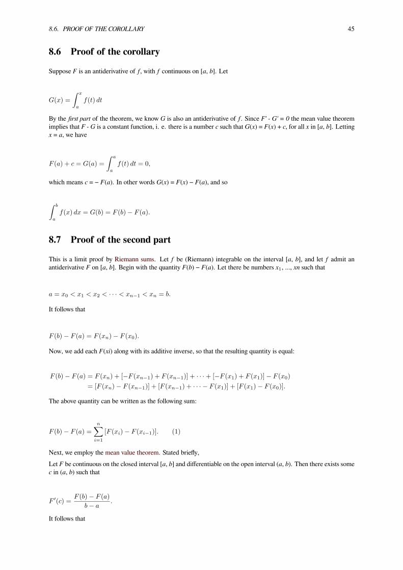
8.6. PROOF OF THE COROLLARY 45
8.6 Proof of the corollary
Suppose F is an antiderivative of f, with f continuous on [a, b]. Let
G(x) =
∫ x
a
f(t) dt
By the first part of the theorem, we know G is also an antiderivative of f. Since F' - G' = 0 the mean value theoremimplies that F - G is a constant function, i. e. there is a number c such that G(x) = F(x) + c, for all x in [a, b]. Lettingx = a, we have
F (a) + c = G(a) =
∫ a
a
f(t) dt = 0,
which means c = − F(a). In other words G(x) = F(x) − F(a), and so
∫ b
a
f(x) dx = G(b) = F (b)− F (a).
8.7 Proof of the second part
This is a limit proof by Riemann sums. Let f be (Riemann) integrable on the interval [a, b], and let f admit anantiderivative F on [a, b]. Begin with the quantity F(b) − F(a). Let there be numbers x1, ..., xn such that
a = x0 < x1 < x2 < · · · < xn−1 < xn = b.
It follows that
F (b)− F (a) = F (xn)− F (x0).
Now, we add each F(xi) along with its additive inverse, so that the resulting quantity is equal:
F (b)− F (a) = F (xn) + [−F (xn−1) + F (xn−1)] + · · ·+ [−F (x1) + F (x1)]− F (x0)
= [F (xn)− F (xn−1)] + [F (xn−1) + · · · − F (x1)] + [F (x1)− F (x0)].
The above quantity can be written as the following sum:
F (b)− F (a) =n∑
i=1
[F (xi)− F (xi−1)]. (1)
Next, we employ the mean value theorem. Stated briefly,Let F be continuous on the closed interval [a, b] and differentiable on the open interval (a, b). Then there exists somec in (a, b) such that
F ′(c) =F (b)− F (a)
b− a.
It follows that
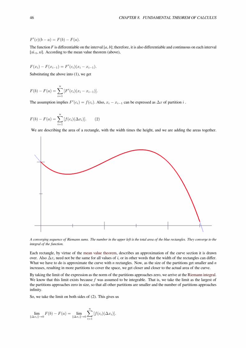
46 CHAPTER 8. FUNDAMENTAL THEOREM OF CALCULUS
F ′(c)(b− a) = F (b)− F (a).
The function F is differentiable on the interval [a, b]; therefore, it is also differentiable and continuous on each interval[xi₋₁, xi]. According to the mean value theorem (above),
F (xi)− F (xi−1) = F ′(ci)(xi − xi−1).
Substituting the above into (1), we get
F (b)− F (a) =n∑
i=1
[F ′(ci)(xi − xi−1)].
The assumption implies F ′(ci) = f(ci). Also, xi − xi−1 can be expressed as ∆x of partition i .
F (b)− F (a) =
n∑i=1
[f(ci)(∆xi)]. (2)
We are describing the area of a rectangle, with the width times the height, and we are adding the areas together.
A converging sequence of Riemann sums. The number in the upper left is the total area of the blue rectangles. They converge to theintegral of the function.
Each rectangle, by virtue of the mean value theorem, describes an approximation of the curve section it is drawnover. Also∆xi need not be the same for all values of i, or in other words that the width of the rectangles can differ.What we have to do is approximate the curve with n rectangles. Now, as the size of the partitions get smaller and nincreases, resulting in more partitions to cover the space, we get closer and closer to the actual area of the curve.By taking the limit of the expression as the norm of the partitions approaches zero, we arrive at the Riemann integral.We know that this limit exists because f was assumed to be integrable. That is, we take the limit as the largest ofthe partitions approaches zero in size, so that all other partitions are smaller and the number of partitions approachesinfinity.So, we take the limit on both sides of (2). This gives us
lim∥∆xi∥→0
F (b)− F (a) = lim∥∆xi∥→0
n∑i=1
[f(ci)(∆xi)].

8.8. EXAMPLES 47
Neither F(b) nor F(a) is dependent on ∥∆xi∥ , so the limit on the left side remains F(b) − F(a).
F (b)− F (a) = lim∥∆xi∥→0
n∑i=1
[f(ci)(∆xi)].
The expression on the right side of the equation defines the integral over f from a to b. Therefore, we obtain
F (b)− F (a) =
∫ b
a
f(x) dx,
which completes the proof.It almost looks like the first part of the theorem follows directly from the second. That is, supposeG is an antiderivativeof f. Then by the second theorem,G(x)−G(a) =
∫ x
af(t) dt . Now, suppose F (x) =
∫ x
af(t) dt = G(x)−G(a)
. Then F has the same derivative as G, and therefore F′ = f. This argument only works, however, if we already knowthat f has an antiderivative, and the only way we know that all continuous functions have antiderivatives is by the firstpart of the Fundamental Theorem.[8] For example if f(x) = e−x2 , then f has an antiderivative, namely
G(x) =
∫ x
0
f(t) dt
and there is no simpler expression for this function. It is therefore important not to interpret the second part of thetheorem as the definition of the integral. Indeed, there are many functions that are integrable but lack antiderivatives.Conversely, many functions that have antiderivatives are not Riemann integrable (see Volterra’s function).
8.8 Examples
As an example, suppose the following is to be calculated:
∫ 5
2
x2 dx.
Here, f(x) = x2 and we can use F (x) = x3
3 as the antiderivative. Therefore:
∫ 5
2
x2 dx = F (5)− F (2) =53
3− 23
3=
125
3− 8
3=
117
3= 39.
Or, more generally, suppose that
d
dx
∫ x
0
t3 dt
is to be calculated. Here, f(t) = t3 and F (t) = t4
4 can be used as the antiderivative. Therefore:
d
dx
∫ x
0
t3 dt =d
dxF (x)− d
dxF (0) =
d
dx
x4
4= x3.
Or, equivalently,
d
dx
∫ x
0
t3 dt = f(x)dx
dx− f(0)
d0
dx= x3.

48 CHAPTER 8. FUNDAMENTAL THEOREM OF CALCULUS
8.9 Generalizations
We don't need to assume continuity of f on the whole interval. Part I of the theorem then says: if f is any Lebesgueintegrable function on [a, b] and x0 is a number in [a, b] such that f is continuous at x0, then
F (x) =
∫ x
a
f(t) dt
is differentiable for x = x0 with F′(x0) = f(x0). We can relax the conditions on f still further and suppose that it ismerely locally integrable. In that case, we can conclude that the function F is differentiable almost everywhere andF′(x) = f(x) almost everywhere. On the real line this statement is equivalent to Lebesgue’s differentiation theorem.These results remain true for the Henstock–Kurzweil integral, which allows a larger class of integrable functions(Bartle 2001, Thm. 4.11).In higher dimensions Lebesgue’s differentiation theorem generalizes the Fundamental theorem of calculus by statingthat for almost every x, the average value of a function f over a ball of radius r centered at x tends to f(x) as r tendsto 0.Part II of the theorem is true for any Lebesgue integrable function f, which has an antiderivative F (not all integrablefunctions do, though). In other words, if a real function F on [a, b] admits a derivative f(x) at every point x of [a, b]and if this derivative f is Lebesgue integrable on [a, b], then
F (b)− F (a) =∫ b
af(t) dt. [9]
This result may fail for continuous functions F that admit a derivative f(x) at almost every point x, as the exampleof the Cantor function shows. However, if F is absolutely continuous, it admits a derivative F′ (x) at almost everypoint x, and moreover F′ is integrable, with F(b) − F(a) equal to the integral of F′ on [a, b]. Conversely, if f is anyintegrable function, then F as given in the first formula will be absolutely continuous with F′ = f a.e.The conditions of this theorem may again be relaxed by considering the integrals involved as Henstock–Kurzweilintegrals. Specifically, if a continuous function F(x) admits a derivative f(x) at all but countably many points, thenf(x) is Henstock–Kurzweil integrable and F(b) − F(a) is equal to the integral of f on [a, b]. The difference here isthat the integrability of f does not need to be assumed. (Bartle 2001, Thm. 4.7)The version of Taylor’s theorem, which expresses the error term as an integral, can be seen as a generalization of theFundamental Theorem.There is a version of the theorem for complex functions: suppose U is an open set in C and f : U → C is a functionthat has a holomorphic antiderivative F onU. Then for every curve γ : [a, b] →U, the curve integral can be computedas
∫γ
f(z) dz = F (γ(b))− F (γ(a)).
The fundamental theorem can be generalized to curve and surface integrals in higher dimensions and on manifolds.One such generalization offered by the calculus of moving surfaces is the time evolution of integrals. The mostfamiliar extensions of the Fundamental theorem of calculus in higher dimensions are the Divergence theorem and theGradient theorem.One of the most powerful statements in this direction is Stokes’ theorem: Let M be an oriented piecewise smoothmanifold of dimension n and let ω be an n−1 form that is a compactly supported differential form on M of class C1.If ∂M denotes the boundary of M with its induced orientation, then
∫M
dω =
∮∂M
ω.
Here d is the exterior derivative, which is defined using the manifold structure only.The theorem is often used in situations where M is an embedded oriented submanifold of some bigger manifold onwhich the form ω is defined.

8.10. SEE ALSO 49
8.10 See also• Differentiation under the integral sign
• Telescoping series
8.11 Notes[1] More exactly, the theorem deals with definite integration with variable upper limit and arbitrarily selected lower limit. This
particular kind of definite integration allows us to compute one of the infinitely many antiderivatives of a function (exceptfor those that do not have a zero). Hence, it is almost equivalent to indefinite integration, defined by most authors as anoperation that yields any one of the possible antiderivatives of a function, including those without a zero.
[2] Spivak, Michael (1980), Calculus (2nd ed.), Houston, Texas: Publish or Perish Inc.
[3] See, e.g., Marlow Anderson, Victor J. Katz, Robin J. Wilson, Sherlock Holmes in Babylon and Other Tales of MathematicalHistory, Mathematical Association of America, 2004, p. 114.
[4] https://archive.org/details/geometricallectu00barruoft
[5] Bers, Lipman. Calculus, pp. 180-181 (Holt, Rinehart and Winston (1976).
[6] Apostol 1967, §5.1
[7] Apostol 1967, §5.3
[8] Spivak, Michael (1980), Calculus (2nd ed.), Houston, Texas: Publish or Perish Inc.
[9] Rudin 1987, th. 7.21
8.12 References• Apostol, Tom M. (1967), Calculus, Vol. 1: One-Variable Calculus with an Introduction to Linear Algebra (2nded.), New York: John Wiley & Sons, ISBN 978-0-471-00005-1.
• Bartle, Robert (2001), A Modern Theory of Integration, AMS, ISBN 0-8218-0845-1.
• Larson, Ron; Edwards, Bruce H.; Heyd, David E. (2002), Calculus of a single variable (7th ed.), Boston:Houghton Mifflin Company, ISBN 978-0-618-14916-2.
• Leithold, L. (1996), The calculus of a single variable (6th ed.), New York: HarperCollins College Publishers.
• Malet, A, Studies on James Gregorie (1638-1675) (PhD Thesis, Princeton, 1989).
• Rudin, Walter (1987), Real and Complex Analysis (third ed.), New York: McGraw-Hill Book Co., ISBN0-07-054234-1
• Stewart, J. (2003), “Fundamental Theorem of Calculus”, Calculus: early transcendentals, Belmont, California:Thomson/Brooks/Cole.
• Turnbull, H. W., ed. (1939), The James Gregory Tercentenary Memorial Volume, London.
• Spivak, Michael (1980), Calculus (2nd ed.), Houston, Texas: Publish or Perish Inc..
• Courant, Richard; John, Fritz (1965), Introduction to Calculus and Analysis, Springer.
8.13 Further reading• Hernandez Rodriguez, O. A.; Lopez Fernandez, J. M. . "Teaching the Fundamental Theorem of Calculus: AHistorical Reflection", Loci: Convergence (MAA), January 2012.
• Fundamental Theorem of Calculus MIT
• Fundamental Theorem of Calculus Mathworld

50 CHAPTER 8. FUNDAMENTAL THEOREM OF CALCULUS
8.14 External links• Hazewinkel, Michiel, ed. (2001), “Fundamental theorem of calculus”, Encyclopedia of Mathematics, Springer,ISBN 978-1-55608-010-4
• James Gregory’s Euclidean Proof of the Fundamental Theorem of Calculus at Convergence
• Isaac Barrow’s proof of the Fundamental Theorem of Calculus
• Fundamental Theorem of Calculus at imomath.com
• Alternative proof the to the fundamental theorem of calculus

Chapter 9
Gradient theorem
The gradient theorem, also known as the fundamental theorem of calculus for line integrals, says that a lineintegral through a gradient field can be evaluated by evaluating the original scalar field at the endpoints of the curve.Let φ : U ⊆ Rn → R . Then
φ (q)− φ (p) =∫γ[p, q]
∇φ(r) · dr.
It is a generalization of the fundamental theorem of calculus to any curve in a plane or space (generally n-dimensional)rather than just the real line.The gradient theorem implies that line integrals through gradient fields are path independent. In physics this theoremis one of the ways of defining a “conservative” force. By placing φ as potential, ∇φ is a conservative field. Workdone by conservative forces does not depend on the path followed by the object, but only the end points, as the aboveequation shows.The gradient theorem also has an interesting converse: any path-independent vector field can be expressed as thegradient of a scalar field. Just like the gradient theorem itself, this converse has many striking consequences andapplications in both pure and applied mathematics.
9.1 Proof
If φ is a differentiable function from some open subset U (of Rn) to R, and if r is a differentiable function from someclosed interval [a,b] to U, then by the multivariate chain rule, the composite function φ ∘ r is differentiable on (a, b)and
d
dt(φ r)(t) = ∇φ(r(t)) · r′(t)
for all t in (a, b). Here the ⋅ denotes the usual inner product.Now suppose the domain U of φ contains the differentiable curve γ with endpoints p and q, (oriented in the directionfrom p to q). If r parametrizes γ for t in [a, b], then the above shows that [1]
∫γ
∇φ(u) · du =
∫ b
a
∇φ(r(t)) · r′(t)dt
=
∫ b
a
d
dtφ(r(t))dt = φ(r(b))− φ(r(a)) = φ (q)− φ (p)
where the definition of the line integral is used in the first equality, and the fundamental theorem of calculus is usedin the third equality.
51

52 CHAPTER 9. GRADIENT THEOREM
9.2 Examples
9.2.1 Example 1
Suppose γ ⊂ R2 is the circular arc oriented counterclockwise from (5, 0) to (−4, 3). Using the definition of a lineintegral,
∫γ
ydx+ xdy =
∫ π−tan−1( 34 )
0
(5 sin t(−5 sin t) + 5 cos t(5 cos t))dt
=
∫ π−tan−1( 34 )
0
25(−sin2t+ cos2t)dt
=
∫ π−tan−1( 34 )
0
25 cos(2t)dt
= 252 sin(2t)
∣∣π−tan−1(34 )
0
= 252 sin(2π − 2tan−1( 34 ))
= −252 sin(2tan−1( 34 ))
= −25( 34 )
( 34 )2+ 1
= −12.
Notice all of the painstaking computations involved in directly calculating the integral. Instead, since the functionf(x, y) = xy is differentiable on all of R2, we can simply use the gradient theorem to say
∫γ
ydx+ xdy =
∫γ
∇(xy) · (dx, dy) = xy|(−4,3)(5,0) = −4 · 3− 5 · 0 = −12
Notice that either way gives the same answer, but using the latter method, most of the work is already done in theproof of the gradient theorem.
9.2.2 Example 2
For a more abstract example, suppose γ ⊂ Rn has endpoints p, q, with orientation from p to q. For u in Rn, let |u|denote the Euclidean norm of u. If α ≥ 1 is a real number, then
∫γ
|x|α−1x · dx =1
α+ 1
∫γ
(α+ 1)|x|(α+1)−2x · dx
=1
α+ 1
∫γ
∇(|x|α+1) · dx =|q|α+1 − |p|α+1
α+ 1
Here the final equality follows by the gradient theorem, since the function f(x) = |x|α + 1 is differentiable on Rn if α ≥1.If α < 1 then this equality will still hold in most cases, but caution must be taken if γ passes through or encloses theorigin, because the integrand vector field |x|α−1x will fail to be defined there. However, the case α = −1 is somewhatdifferent; in this case, the integrand becomes |x|−2x = ∇(log|x|), so that the final equality becomes log|q|−log|p|.Note that if n=1, then this example is simply a slight variant of the familiar Power rule from single-variable calculus.
9.2.3 Example 3
Suppose there are n point charges arranged in three-dimensional space, and the i-th point charge has charge Qi andis located at position pi in R3. We would like to calculate the work done on a particle of charge q as it travels from a

9.3. CONVERSE OF THE GRADIENT THEOREM 53
point a to a point b in R3. Using Coulomb’s law, we can easily determine that the force on the particle at position rwill be
F(r) = kq
n∑i=1
Qi(r− pi)|r− pi|3
Here |u| denotes the Euclidean norm of the vector u in R3, and k = 1/(4πε0), where ε0 is the Vacuum permittivity.Let γ ⊂ R3 − p1, ..., pn be an arbitrary differentiable curve from a to b. Then the work done on the particle is
W =
∫γ
F(r) · dr =∫γ
(kq
n∑i=1
Qi(r− pi)|r− pi|3
)· dr = kq
n∑i=1
(Qi
∫γ
(r− pi)|r− pi|3
· dr)
Now for each i, direct computation shows that
(r− pi)|r− pi|3
= −∇(
1
|r− pi|
).
Thus, continuing from above and using the gradient theorem,
W = −kqn∑
i=1
(Qi
∫γ
∇(
1
|r− pi|
)· dr)
= kqn∑
i=1
Qi
(1
|a− pi|− 1
|b− pi|
)Weare finished. Of course, we could have easily completed this calculation using the powerful language of electrostaticpotential or electrostatic potential energy (with the familiar formulasW = −ΔU = −qΔV). However, we have not yetdefined potential or potential energy, because the converse of the gradient theorem is required to prove that these arewell-defined, differentiable functions and that these formulas hold (see below). Thus, we have solved this problemusing only Coulomb’s Law, the definition of work, and the gradient theorem.
9.3 Converse of the gradient theorem
The gradient theorem states that if the vector field F is the gradient of some scalar-valued function (i.e, if F isconservative), then F is a path-independent vector field (i.e, the integral of F over some piecewise-differentiablecurve is dependent only on end points). This theorem has a powerful converse; namely, if F is a path-independentvector field, then F is the gradient of some scalar-valued function.[2] It is straightforward to show that a vector field ispath-independent if and only if the integral of the vector field over every closed loop in its domain is zero. Thus theconverse can alternatively be stated as follows: If the integral of F over every closed loop in the domain of F is zero,then F is the gradient of some scalar-valued function.
9.3.1 Example of the converse principle
Main article: Electric potential energy
To illustrate the power of this converse principle, we cite an example that has significant physical consequences. Inclassical electromagnetism, the electric force is a path-independent force ; i.e. the work done on a particle that hasreturned to its original position within an electric field is zero (assuming that no changing magnetic fields are present).Therefore the above theorem implies that the electric force field Fe : S → R3 is conservative (here S is some open,path-connected subset of R3 that contains a charge distribution). Following the ideas of the above proof, we can setsome reference point a in S, and define a function Ue: S → R by
Ue(r) := −∫γ[a,r]
Fe(u) · du
54 CHAPTER 9. GRADIENT THEOREM
Using the above proof, we know Ue is well-defined and differentiable, and Fe = −∇Ue (from this formula we can usethe gradient theorem to easily derive the well-known formula for calculating work done by conservative forces: W =−ΔU). This function Ue is often referred to as the electrostatic potential energy of the system of charges in S (withreference to the zero-of-potential a). In many cases, the domain S is assumed to be unbounded and the reference pointa is taken to be “infinity,” which can be made rigorous using limiting techniques. This functionUe is an indispensabletool used in the analysis of many physical systems.
9.4 Generalizations
Main articles: Stokes’ theorem and Closed and exact differential forms
Many of the critical theorems of vector calculus generalize elegantly to statements about the integration of differentialforms on manifolds. In the language of differential forms and exterior derivatives, the gradient theorem states that
∫∂γ
ϕ =
∫γ
dϕ
for any 0-form φ defined on some differentiable curve γ ⊂ Rn (here the integral of φ over the boundary of the γ isunderstood to be the evaluation of φ at the endpoints of γ).Notice the striking similarity between this statement and the generalized version of Stokes’ theorem, which says thatthe integral of any compactly supported differential form ω over the boundary of some orientable manifold Ω is equalto the integral of its exterior derivative dω over the whole of Ω, i.e.
∫∂Ω
ω =
∫Ω
dω
This powerful statement is a generalization of the gradient theorem from 1-forms defined on one-dimensional mani-folds to differential forms defined on manifolds of arbitrary dimension.The converse statement of the gradient theorem also has a powerful generalization in terms of differential forms onmanifolds. In particular, suppose ω is a form defined on a contractible domain, and the integral of ω over any closedmanifold is zero. Then there exists a form ψ such that ω = dψ. Thus, on a contractible domain, every closed form isexact. This result is summarized by the Poincaré lemma.
9.5 See also• State function
• Scalar potential
• Jordan curve theorem
• Differential of a function
• Classical mechanics
9.6 References[1] Williamson, Richard and Trotter, Hale. (2004). Multivariable Mathematics, Fourth Edition, p. 374. Pearson Education,
Inc.
[2] Williamson, Richard and Trotter, Hale. (2004). Multivariable Mathematics, Fourth Edition, p. 410. Pearson Education,Inc.

Chapter 10
Green’s theorem
This article is about the theorem in the plane relating double integrals and line integrals. For Green’s theorems relat-ing volume integrals involving the Laplacian to surface integrals, see Green’s identities.
In mathematics,Green’s theorem gives the relationship between a line integral around a simple closed curve C and adouble integral over the plane region D bounded by C. It is named after George Green [1] and is the two-dimensionalspecial case of the more general Kelvin–Stokes theorem.
10.1 Theorem
Let C be a positively oriented, piecewise smooth, simple closed curve in a plane, and let D be the region bounded byC. If L and M are functions of (x, y) defined on an open region containing D and have continuous partial derivativesthere, then[2][3]
∮C
(Ldx+M dy) =
∫∫D
(∂M
∂x− ∂L
∂y
)dx dy
where the path of integration along C is counterclockwise.In physics, Green’s theorem is mostly used to solve two-dimensional flow integrals, stating that the sum of fluidoutflows from a volume is equal to the total outflow summed about an enclosing area. In plane geometry, and inparticular, area surveying, Green’s theorem can be used to determine the area and centroid of plane figures solely byintegrating over the perimeter.
10.2 Proof when D is a simple region
The following is a proof of half of the theorem for the simplified area D, a type I region where C1 and C3 are curvesconnected by vertical lines (possibly of zero length). A similar proof exists for the other half of the theorem when Dis a type II region where C2 and C4 are curves connected by horizontal lines (again, possibly of zero length). Puttingthese two parts together, the theorem is thus proven for regions of type III (defined as regions which are both typeI and type II). The general case can then be deduced from this special case by decomposing D into a set of type IIIregions.If it can be shown that
∮C
Ldx =
∫∫D
(−∂L∂y
)dA (1)
and
55

56 CHAPTER 10. GREEN’S THEOREM
y
xa b
DC
C
C C
1
4
3
2
If D is a simple region with its boundary consisting of the curves C1, C2, C3, C4, half of Green’s theorem can be demonstrated.
∮C
M dy =
∫∫D
(∂M
∂x
)dA (2)
are true, then Green’s theorem follows immediately for the region D. We can prove (1) easily for regions of type I,and (2) for regions of type II. Green’s theorem then follows for regions of type III.Assume region D is a type I region and can thus be characterized, as pictured on the right, by
D = (x, y)|a ≤ x ≤ b, g1(x) ≤ y ≤ g2(x)
where g1 and g2 are continuous functions on [a, b]. Compute the double integral in (1):
∫∫D
∂L
∂ydA =
∫ b
a
∫ g2(x)
g1(x)
∂L
∂y(x, y) dy dx
=
∫ b
a
L(x, g2(x))− L(x, g1(x))
dx. (3)
10.3. RELATIONSHIP TO THE STOKES THEOREM 57
Now compute the line integral in (1). C can be rewritten as the union of four curves: C1, C2, C3, C4.With C1, use the parametric equations: x = x, y = g1(x), a ≤ x ≤ b. Then
∫C1
L(x, y) dx =
∫ b
a
L(x, g1(x)) dx.
With C3, use the parametric equations: x = x, y = g2(x), a ≤ x ≤ b. Then
∫C3
L(x, y) dx = −∫−C3
L(x, y) dx = −∫ b
a
L(x, g2(x)) dx.
The integral over C3 is negated because it goes in the negative direction from b to a, as C is oriented positively(counterclockwise). On C2 and C4, x remains constant, meaning
∫C4
L(x, y) dx =
∫C2
L(x, y) dx = 0.
Therefore,
∫C
Ldx =
∫C1
L(x, y) dx+
∫C2
L(x, y) dx+
∫C3
L(x, y) dx+
∫C4
L(x, y) dx
= −∫ b
a
L(x, g2(x)) dx+
∫ b
a
L(x, g1(x)) dx. (4)
Combining (3) with (4), we get (1) for regions of type I. A similar treatment yields (2) for regions of type II. Puttingthe two together, we get the result for regions of type III.
10.3 Relationship to the Stokes theorem
Green’s theorem is a special case of the Kelvin–Stokes theorem, when applied to a region in the xy-plane:We can augment the two-dimensional field into a three-dimensional field with a z component that is always 0. WriteF for the vector-valued function F = (L,M, 0) . Start with the left side of Green’s theorem:
∮C
(Ldx+M dy) =
∮C
(L,M, 0) · (dx, dy, dz) =∮C
F · dr.
Kelvin–Stokes Theorem:
∮C
F · dr =∫∫
S
∇× F · n dS.
The surface S is just the region in the plane D , with the unit normals n pointing up (in the positive z direction) tomatch the “positive orientation” definitions for both theorems.The expression inside the integral becomes
∇× F · n =
[(∂0
∂y− ∂M
∂z
)i+(∂L
∂z− ∂0
∂x
)j+
(∂M
∂x− ∂L
∂y
)k]· k =
(∂M
∂x− ∂L
∂y
).
Thus we get the right side of Green’s theorem

58 CHAPTER 10. GREEN’S THEOREM
∫∫S
∇× F · n dS =
∫∫D
(∂M
∂x− ∂L
∂y
)dA.
Green’s theorem is also a straightforward result of the general Stokes’ theorem using differential forms and exteriorderivatives:
∮C
Ldx+M dy =
∮∂D
ω =
∫D
dω =
∫D
∂L
∂ydy ∧ dx+
∂M
∂xdx ∧ dy =
∫∫D
(∂M
∂x− ∂L
∂y
)dx dy.
10.4 Relationship to the divergence theorem
Considering only two-dimensional vector fields, Green’s theorem is equivalent to the two-dimensional version of thedivergence theorem:
∫∫D
(∇ · F) dA =
∮C
F · n ds,
where∇·F is the divergence on the two-dimensional vector field F , and n is the outward-pointing unit normal vectoron the boundary.To see this, consider the unit normal n in the right side of the equation. Since in Green’s theorem dr = (dx, dy) isa vector pointing tangential along the curve, and the curve C is the positively oriented (i.e. counterclockwise) curvealong the boundary, an outward normal would be a vector which points 90° to the right of this; one choice would be(dy,−dx) . The length of this vector is
√dx2 + dy2 = ds. So (dy,−dx) = n ds.
Start with the left side of Green’s theorem:
∮C
(Ldx+M dy) =
∮C
(M,−L) · (dy,−dx) =∮C
(M,−L) · n ds.
Applying the two-dimensional divergence theorem with F = (M,−L) , we get the right side of Green’s theorem:
∮C
(M,−L) · n ds =∫∫
D
(∇ · (M,−L)) dA =
∫∫D
(∂M
∂x− ∂L
∂y
)dA.
10.5 Area calculation
Green’s theorem can be used to compute area by line integral.[4] The area of D is given by A =∫∫
DdA . Then if
we choose L and M such that ∂M∂x − ∂L
∂y = 1 , the area is given by A =∮C(Ldx+M dy) .
Possible formulas for the area of D include:[4] A =∮Cx dy = −
∮Cy dx = 1
2
∮C(−y dx+ x dy).
10.6 See also
• Planimeter
• Method of image charges – A method used in electrostatics that takes advantage of the uniqueness theorem(derived from Green’s theorem)
• Shoelace formula - A special case of Green’s theorem for simple polygons

10.7. REFERENCES 59
10.7 References[1] George Green, An Essay on the Application of Mathematical Analysis to the Theories of Electricity and Magnetism (Not-
tingham, England: T. Wheelhouse, 1828). Green did not actually derive the form of “Green’s theorem” which appears inthis article; rather, he derived a form of the “divergence theorem”, which appears on pages 10-12 of his Essay.In 1846, the form of “Green’s theorem” which appears in this article was first published, without proof, in an article byAugustin Cauchy: A. Cauchy (1846) “Sur les intégrales qui s’étendent à tous les points d'une courbe fermée” (On integralsthat extend over all of the points of a closed curve), Comptes rendus, 23: 251-255. (The equation appears at the bottom ofpage 254, where (S) denotes the line integral of a function k along the curve s that encloses the area S.)A proof of the theorem was finally provided in 1851 by Bernhard Riemann in his inaugural dissertation: Bernhard Riemann(1851) Grundlagen für eine allgemeine Theorie der Functionen einer veränderlichen complexen Grösse (Basis for a generaltheory of functions of a variable complex quantity), (Göttingen, (Germany): Adalbert Rente, 1867); see pages 8 - 9.
[2] Mathematical methods for physics and engineering, K.F. Riley, M.P. Hobson, S.J. Bence, Cambridge University Press,2010, ISBN 978-0-521-86153-3
[3] Vector Analysis (2nd Edition), M.R. Spiegel, S. Lipschutz, D. Spellman, Schaum’s Outlines, McGraw Hill (USA), 2009,ISBN 978-0-07-161545-7
[4] Stewart, James. Calculus (6th ed.). Thomson, Brooks/Cole.
10.8 Further reading• Ayres, F.; Mendelson, E. (2009). Calculus. Schaum’s Outline (5th ed.). ISBN 978-0-07-150861-2.
• Wrede, R.; Spiegel, M. R. (2010). Advanced Calculus. Schaum’s Outline (3rd ed.). ISBN 978-0-07-162366-7.
10.9 External links• Green’s Theorem on MathWorld
Chapter 11
Implicit function theorem
In multivariable calculus, the implicit function theorem, also known, especially in Italy, asDini's theorem, is a toolthat allows relations to be converted to functions of several real variables. It does this by representing the relation asthe graph of a function. There may not be a single function whose graph is the entire relation, but there may be sucha function on a restriction of the domain of the relation. The implicit function theorem gives a sufficient condition toensure that there is such a function.The theorem states that if the equation F(x1, ..., xn, y1, ..., ym) = F(x, y) = 0 satisfies some mild conditions onits partial derivatives, then one can in principle (though not necessarily with an analytic expression) express the mvariables yi in terms of the n variables xj as yi = fi (x), at least in some disk. Then each of these implicit functions fi(x),[1]:204-206 implied by F(x, y) = 0, is such that geometrically the locus defined by F(x, y) = 0 will coincide locally(that is in that disk) with the hypersurface given by y = f(x).
11.1 First example
If we define the function f(x, y) = x2 + y2 , then the equation f(x, y) = 1 cuts out the unit circle as the level set(x, y)| f(x, y) = 1. There is no way to represent the unit circle as the graph of a function of one variable y = g(x)because for each choice of x ∈ (−1, 1), there are two choices of y, namely ±
√1− x2 .
However, it is possible to represent part of the circle as the graph of a function of one variable. If we let g1(x) =√1− x2 for −1 < x < 1, then the graph of y = g1(x) provides the upper half of the circle. Similarly, if g2(x) =
−√1− x2 , then the graph of y = g2(x) gives the lower half of the circle.
The purpose of the implicit function theorem is to tell us the existence of functions like g1(x) and g2(x) , even insituations where we cannot write down explicit formulas. It guarantees that g1(x) and g2(x) are differentiable, andit even works in situations where we do not have a formula for f(x, y).
11.2 Definitions
Let f : Rn+m → Rm be a continuously differentiable function. We think of Rn+m as the Cartesian product Rn × Rm,and we write a point of this product as (x, y) = (x1, ..., xn, y1, ..., ym). Starting from the given function f, our goal isto construct a function g: Rn → Rm whose graph (x, g(x)) is precisely the set of all (x, y) such that f(x, y) = 0.As noted above, this may not always be possible. We will therefore fix a point (a, b) = (a1, ..., an, b1, ..., bm) whichsatisfies f(a, b) = 0, and we will ask for a g that works near the point (a, b). In other words, we want an open set Uof Rn containing a, an open set V of Rm containing b, and a function g : U → V such that the graph of g satisfies therelation f = 0 on U × V. In symbols,
(x, g(x)) | x ∈ U = (x, y) ∈ U × V | f(x, y) = 0.
To state the implicit function theorem, we need the Jacobian matrix of f, which is the matrix of the partial derivativesof f. Abbreviating (a1, ..., an, b1, ..., bm) to (a, b), the Jacobian matrix is
60

11.3. STATEMENT OF THE THEOREM 61
A
B
The unit circle can be specified as the level curve f(x, y) = 1 of the function f(x, y) = x2+y2 . Around point A, y can be expressedas a function y(x), specifically g1(x) =
√1− x2 . No such function exists around point B.
(Df)(a, b) =
∂f1∂x1
(a, b) · · · ∂f1∂xn
(a, b)... . . . ...
∂fm∂x1
(a, b) · · · ∂fm∂xn
(a, b)
∣∣∣∣∣∣∣∂f1∂y1
(a, b) · · · ∂f1∂ym
(a, b)... . . . ...
∂fm∂y1
(a, b) · · · ∂fm∂ym
(a, b)
= [X|Y ]
where X is the matrix of partial derivatives in the variables xi and Y is the matrix of partial derivatives in the variablesyj. The implicit function theorem says that if Y is an invertible matrix, then there are U, V, and g as desired. Writingall the hypotheses together gives the following statement.
11.3 Statement of the theorem
Let f: Rn+m → Rm be a continuously differentiable function, and let Rn+m have coordinates (x, y). Fix a point (a, b)= (a1, ..., an, b1, ..., bm) with f(a, b) = c, where c ∈ Rm. If the matrix [(∂fi/∂yj)(a, b)] is invertible, then there exists
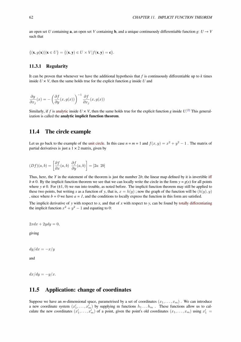
62 CHAPTER 11. IMPLICIT FUNCTION THEOREM
an open set U containing a, an open set V containing b, and a unique continuously differentiable function g: U → Vsuch that
(x, g(x))|x ∈ U = (x, y) ∈ U × V |f(x, y) = c.
11.3.1 Regularity
It can be proven that whenever we have the additional hypothesis that f is continuously differentiable up to k timesinside U × V, then the same holds true for the explicit function g inside U and
∂g
∂xj(x) = −
(∂f
∂y(x, g(x))
)−1∂f
∂xj(x, g(x))
Similarly, if f is analytic inside U × V, then the same holds true for the explicit function g inside U.[2] This general-ization is called the analytic implicit function theorem.
11.4 The circle example
Let us go back to the example of the unit circle. In this case n = m = 1 and f(x, y) = x2 + y2 − 1 . The matrix ofpartial derivatives is just a 1 × 2 matrix, given by
(Df)(a, b) =
[∂f
∂x(a, b)
∂f
∂y(a, b)
]= [2a 2b]
Thus, here, the Y in the statement of the theorem is just the number 2b; the linear map defined by it is invertible iffb ≠ 0. By the implicit function theorem we see that we can locally write the circle in the form y = g(x) for all pointswhere y ≠ 0. For (±1, 0) we run into trouble, as noted before. The implicit function theorem may still be applied tothese two points, but writing x as a function of y, that is, x = h(y) ; now the graph of the function will be (h(y), y), since where b = 0 we have a = 1, and the conditions to locally express the function in this form are satisfied.The implicit derivative of y with respect to x, and that of x with respect to y, can be found by totally differentiatingthe implicit function x2 + y2 − 1 and equating to 0:
2xdx+ 2ydy = 0,
giving
dy/dx = −x/y
and
dx/dy = −y/x.
11.5 Application: change of coordinates
Suppose we have an m-dimensional space, parametrised by a set of coordinates (x1, . . . , xm) . We can introducea new coordinate system (x′1, . . . , x
′m) by supplying m functions h1 . . . hm . These functions allow us to cal-
culate the new coordinates (x′1, . . . , x′m) of a point, given the point’s old coordinates (x1, . . . , xm) using x′1 =
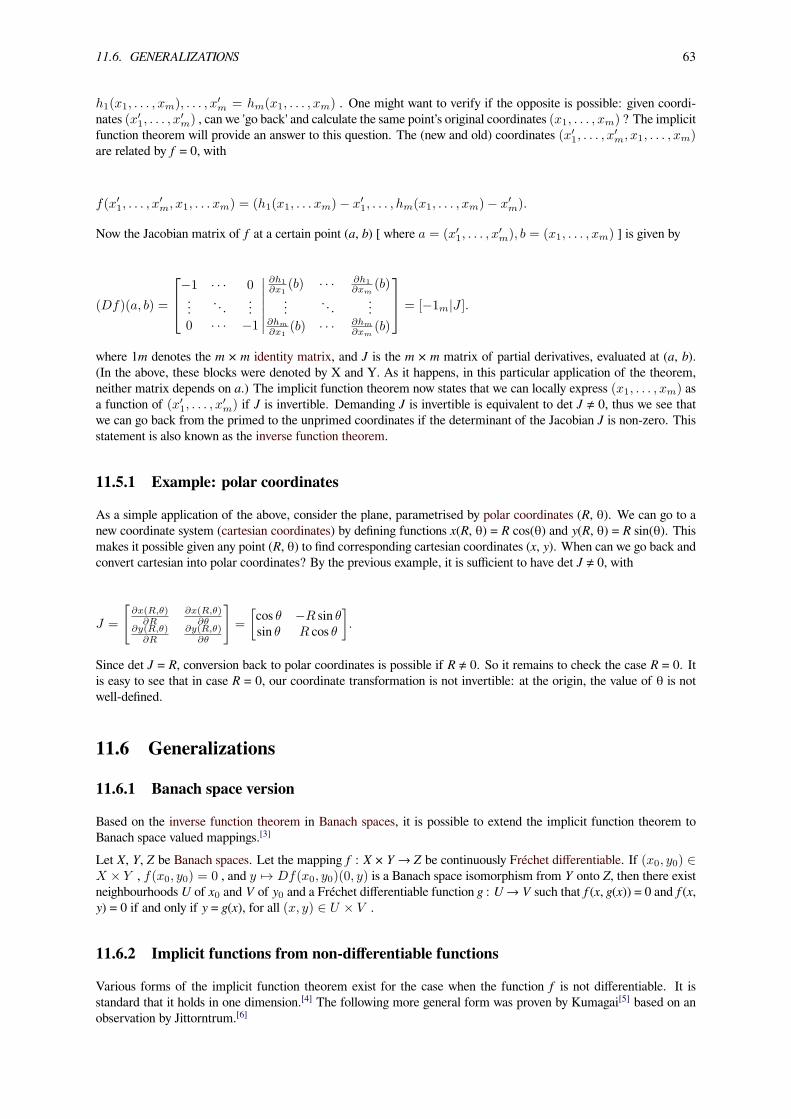
11.6. GENERALIZATIONS 63
h1(x1, . . . , xm), . . . , x′m = hm(x1, . . . , xm) . One might want to verify if the opposite is possible: given coordi-nates (x′1, . . . , x′m) , can we 'go back' and calculate the same point’s original coordinates (x1, . . . , xm) ? The implicitfunction theorem will provide an answer to this question. The (new and old) coordinates (x′1, . . . , x′m, x1, . . . , xm)are related by f = 0, with
f(x′1, . . . , x′m, x1, . . . xm) = (h1(x1, . . . xm)− x′1, . . . , hm(x1, . . . , xm)− x′m).
Now the Jacobian matrix of f at a certain point (a, b) [ where a = (x′1, . . . , x′m), b = (x1, . . . , xm) ] is given by
(Df)(a, b) =
−1 · · · 0... . . . ...0 · · · −1
∣∣∣∣∣∣∣∂h1
∂x1(b) · · · ∂h1
∂xm(b)
... . . . ...∂hm
∂x1(b) · · · ∂hm
∂xm(b)
= [−1m|J ].
where 1m denotes the m × m identity matrix, and J is the m × m matrix of partial derivatives, evaluated at (a, b).(In the above, these blocks were denoted by X and Y. As it happens, in this particular application of the theorem,neither matrix depends on a.) The implicit function theorem now states that we can locally express (x1, . . . , xm) asa function of (x′1, . . . , x′m) if J is invertible. Demanding J is invertible is equivalent to det J ≠ 0, thus we see thatwe can go back from the primed to the unprimed coordinates if the determinant of the Jacobian J is non-zero. Thisstatement is also known as the inverse function theorem.
11.5.1 Example: polar coordinates
As a simple application of the above, consider the plane, parametrised by polar coordinates (R, θ). We can go to anew coordinate system (cartesian coordinates) by defining functions x(R, θ) = R cos(θ) and y(R, θ) = R sin(θ). Thismakes it possible given any point (R, θ) to find corresponding cartesian coordinates (x, y). When can we go back andconvert cartesian into polar coordinates? By the previous example, it is sufficient to have det J ≠ 0, with
J =
[∂x(R,θ)
∂R∂x(R,θ)
∂θ∂y(R,θ)
∂R∂y(R,θ)
∂θ
]=
[cos θ −R sin θsin θ R cos θ
].
Since det J = R, conversion back to polar coordinates is possible if R ≠ 0. So it remains to check the case R = 0. Itis easy to see that in case R = 0, our coordinate transformation is not invertible: at the origin, the value of θ is notwell-defined.
11.6 Generalizations
11.6.1 Banach space version
Based on the inverse function theorem in Banach spaces, it is possible to extend the implicit function theorem toBanach space valued mappings.[3]
Let X, Y, Z be Banach spaces. Let the mapping f : X × Y → Z be continuously Fréchet differentiable. If (x0, y0) ∈X × Y , f(x0, y0) = 0 , and y 7→ Df(x0, y0)(0, y) is a Banach space isomorphism from Y onto Z, then there existneighbourhoods U of x0 and V of y0 and a Fréchet differentiable function g : U → V such that f(x, g(x)) = 0 and f(x,y) = 0 if and only if y = g(x), for all (x, y) ∈ U × V .
11.6.2 Implicit functions from non-differentiable functions
Various forms of the implicit function theorem exist for the case when the function f is not differentiable. It isstandard that it holds in one dimension.[4] The following more general form was proven by Kumagai[5] based on anobservation by Jittorntrum.[6]

64 CHAPTER 11. IMPLICIT FUNCTION THEOREM
Consider a continuous function f : Rn × Rm → Rn such that f(x0, y0) = 0 . If there exist open neighbourhoodsA ⊂ Rn and B ⊂ Rm of x0 and y0, respectively, such that, for all y in B, f(·, y) : A → Rn is locally one-to-onethen there exist open neighbourhoods A0 ⊂ Rn and B0 ⊂ Rm of x0 and y0, such that, for all y ∈ B0 , the equationf(x, y) = 0 has a unique solution
x = g(y) ∈ A0
where g is a continuous function from B0 into A0.
11.7 See also• Constant rank theorem: Both the implicit function theorem and the Inverse function theorem can be seen asspecial cases of the constant rank theorem.
11.8 Notes[1] Chiang, Alpha C. Fundamental Methods of Mathematical Economics, McGraw-Hill, third edition, 1984
[2] K. Fritzsche, H. Grauert (2002), “From Holomorphic Functions to Complex Manifolds”, Springer-Verlag, page 34.
[3] Lang 1999, pp. 15–21. Edwards 1994, pp. 417–418.
[4] Kudryavtsev, L. D. (1990). “Implicit function”. In Hazewinkel, M. Encyclopedia of Mathematics. Dordrecht, The Nether-lands: Kluwer. ISBN 1-55608-004-2.
[5] Kumagai, S. (June 1980). “An implicit function theorem: Comment”. Journal of Optimization Theory and Applications31 (2): 285–288. doi:10.1007/BF00934117.
[6] Jittorntrum, K. (1978). “An Implicit Function Theorem”. Journal of Optimization Theory and Applications 25 (4): 575–577. doi:10.1007/BF00933522.
11.9 References• Danilov, V.I. (2001), “Implicit function (in algebraic geometry)", in Hazewinkel, Michiel, Encyclopedia of
Mathematics, Springer, ISBN 978-1-55608-010-4
• Edwards, Charles Henry (1994) [1973]. Advanced calculus of several variables. Mineola, New York: DoverPublications. ISBN 978-0-486-68336-2.
• Kudryavtsev, L.D. (2001), “Implicit function”, in Hazewinkel, Michiel, Encyclopedia ofMathematics, Springer,ISBN 978-1-55608-010-4
• Lang, Serge (1999). Fundamentals of Differential Geometry. Graduate Texts in Mathematics. New York:Springer. ISBN 978-0-387-98593-0.

Chapter 12
Intermediate value theorem
Not to be confused with the Mean value theorem.
In mathematical analysis, the intermediate value theorem states that if a continuous function f with an interval [a,b] as its domain takes values f(a) and f(b) at each end of the interval, then it also takes any value between f(a) andf(b) at some point within the interval.This has two important specializations: 1) If a continuous function has values of opposite sign inside an interval, thenit has a root in that interval (Bolzano’s theorem).[1] 2) The image of a continuous function over an interval is itselfan interval.
12.1 Motivation
This captures an intuitive property of continuous functions: given f continuous on [1, 2] with the known values f(1)= 3 and f(2) = 5. Then the graph of y = f(x) must pass through the horizontal line y = 4 while x moves from 1 to 2.It represents the idea that the graph of a continuous function on a closed interval can be drawn without lifting yourpencil from the paper.
12.2 Theorem
The intermediate value theorem states the following. Consider an interval I = [a, b] in the real numbers ℝ and acontinuous function f : I → ℝ. Then,
• Version I. if u is a number between f(a) and f(b),
f(a) < u < f(b) (or f(a) > u > f(b) ),then there is a c ∈ (a, b) such that f(c) = u.
• Version II. the image set f(I) is also an interval, and either it contains [f(a), f(b)], or it contains [f(b), f(a)];that is,
f(I) ⊇ [f(a), f(b)] (or f(I) ⊇ [f(b), f(a)] ).
Remark: Version II states that the set of function values has no gap. For any two function values c<d, even if theyare outside the interval between f(a) and f(b), all points in the interval [c, d] are also function values,
[c, d] ⊆ f(I).
A subset of the real numbers with no internal gap is an interval. Version I is obviously contained in Version II.
65
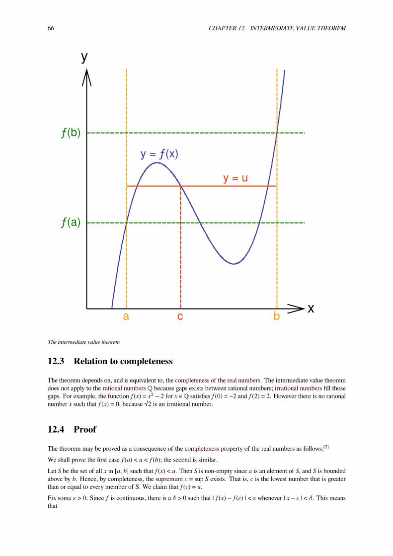
66 CHAPTER 12. INTERMEDIATE VALUE THEOREM
y
x
y = ƒ(x)
a b
y = u
c
ƒ(a)
ƒ(b)
The intermediate value theorem
12.3 Relation to completeness
The theorem depends on, and is equivalent to, the completeness of the real numbers. The intermediate value theoremdoes not apply to the rational numbers ℚ because gaps exists between rational numbers; irrational numbers fill thosegaps. For example, the function f(x) = x2 − 2 for x ∈ ℚ satisfies f(0) = −2 and f(2) = 2. However there is no rationalnumber x such that f(x) = 0, because √2 is an irrational number.
12.4 Proof
The theorem may be proved as a consequence of the completeness property of the real numbers as follows:[2]
We shall prove the first case f(a) < u < f(b); the second is similar.Let S be the set of all x in [a, b] such that f(x) < u. Then S is non-empty since a is an element of S, and S is boundedabove by b. Hence, by completeness, the supremum c = sup S exists. That is, c is the lowest number that is greaterthan or equal to every member of S. We claim that f(c) = u.Fix some ε > 0. Since f is continuous, there is a δ > 0 such that | f(x) − f(c) | < ε whenever | x − c | < δ. This meansthat

12.5. HISTORY 67
f(x) − ε < f(c) < f(x) + ε
for all x between c − δ and c + δ. By the properties of the supremum, there exist a* between c − δ and c that iscontained in S, so that for that a*
f(c) < f(a*) + ε < u + ε.
Choose a** between c and c + δ that will obviously not be contained in S, so we have
f(c) > f(a**) − ε ≥ u − ε.
Both inequalities
u − ε < f(c) < u + ε
are valid for all ε > 0, from which we deduce f(c) = u as the only possible value, as stated.An alternative proof may be found at non-standard calculus.
12.5 History
For u = 0 above, the statement is also known as Bolzano’s theorem. This theorem was first proved by Bernard Bolzanoin 1817. Augustin-Louis Cauchy provided a proof in 1821.[3] Both were inspired by the goal of formalizing theanalysis of functions and the work of Joseph-Louis Lagrange. The idea that continuous functions possess the inter-mediate value property has an earlier origin. Simon Stevin proved the intermediate value theorem for polynomials(using a cubic as an example) by providing an algorithm for constructing the decimal expansion of the solution. Thealgorithm iteratively subdivides the interval into 10 parts, producing an additional decimal digit at each step of theiteration.[4] Before the formal definition of continuity was given, the intermediate value property was given as partof the definition of a continuous function. Proponents include Louis Arbogast, who assumed the functions to haveno jumps, satisfy the intermediate value property and have increments whose sizes corresponded to the sizes of theincrements of the variable.[5] Earlier authors held the result to be intuitively obvious, and requiring no proof. Theinsight of Bolzano and Cauchy was to define a general notion of continuity (in terms of infinitesimals in Cauchy’scase, and using real inequalities in Bolzano’s case), and to provide a proof based on such definitions.
12.6 Generalizations
The intermediate value theorem can be seen as a consequence of the following two statements from topology:
• If X and Y are topological spaces, f : X → Y is continuous, and X is connected, then f(X) is connected.
• A subset of ℝ is connected if and only if it is an interval.
The intermediate value theorem generalizes in a natural way: Suppose that X is a connected topological space and(Y, <) is a totally ordered set equipped with the order topology, and let f : X→ Y be a continuous map. If a and b aretwo points in X and u is a point in Y lying between f(a) and f(b) with respect to <, then there exists c in X such thatf(c) = u. The original theorem is recovered by noting that ℝ is connected and that its natural topology is the ordertopology.The Brouwer fixed-point theorem is a related theorem that, in one dimension gives a special case of the intermediatevalue theorem.
68 CHAPTER 12. INTERMEDIATE VALUE THEOREM
12.7 Converse is false
A "Darboux function" is a real-valued function f that has the “intermediate value property”, i.e., that satisfies theconclusion of the intermediate value theorem: for any two values a and b in the domain of f, and any y betweenf(a) and f(b), there is some c between a and b with f(c) = y. The intermediate value theorem says that everycontinuous function is a Darboux function. However, not every Darboux function is continuous; i.e., the converse ofthe intermediate value theorem is false.As an example, take the function f : [0, ∞) → [−1, 1] defined by f(x) = sin(1/x) for x > 0 and f(0) = 0. This functionis not continuous at x = 0 because the limit of f(x) as x tends to 0 does not exist; yet the function has the intermediatevalue property. Another, more complicated example is given by the Conway base 13 function.Historically, this intermediate value property has been suggested as a definition for continuity of real-valued functions;this definition was not adopted.Darboux’s theorem states that all functions that result from the differentiation of some other function on some intervalhave the intermediate value property (even though they need not be continuous).
12.8 Implications of theorem in real world
The theorem implies that on any great circle around the world, the temperature, pressure, elevation, carbon dioxideconcentration, or any other similar scalar quantity which varies continuously, there will always exist two antipodalpoints that share the same value for that variable.Proof: Take f to be any continuous function on a circle. Draw a line through the center of the circle, intersecting itat two opposite points A and B. Let d be defined by the difference f(A) − f(B). If the line is rotated 180 degrees, thevalue −d will be obtained instead. Due to the intermediate value theorem there must be some intermediate rotationangle for which d = 0, and as a consequence f(A) = f(B) at this angle.This is a special case of a more general result called the Borsuk–Ulam theorem.Another generalization for which this holds is for any closed convex n (n > 1) dimensional shape. Specifically, for anycontinuous function whose domain is the given shape, and any point inside the shape (not necessarily its center), thereexist two antipodal points with respect to the given point whose functional value is the same. The proof is identicalto the one given above.The theorem also underpins the explanation of why rotating a wobbly table will bring it to stability (subject to certaineasily met constraints).[6]
12.9 See also
• Mean value theorem
• Hairy ball theorem
• Brouwer fixed point theorem
12.10 References[1] Weisstein, Eric W., “Bolzano’s Theorem”, MathWorld.
[2] Essentially follows Clarke, Douglas A. (1971). Foundations of Analysis. Appleton-Century-Crofts. p. 284.
[3] Grabiner, Judith V. (March 1983). “Who Gave You the Epsilon? Cauchy and the Origins of Rigorous Calculus” (PDF).The American Mathematical Monthly (Mathematical Association of America) 90 (3): 185–194. doi:10.2307/2975545.JSTOR 2975545
[4] Karin Usadi Katz and Mikhail G. Katz (2011) A Burgessian Critique of Nominalistic Tendencies in Contemporary Math-ematics and its Historiography. Foundations of Science. doi:10.1007/s10699-011-9223-1 See link

12.11. EXTERNAL LINKS 69
[5] O'Connor, John J.; Robertson, Edmund F., “Intermediate value theorem”, MacTutor History of Mathematics archive,University of St Andrews.
[6] Keith Devlin (2007) How to stabilize a wobbly table
12.11 External links• Intermediate value Theorem at ProofWiki
• Intermediate value Theorem - Bolzano Theorem at cut-the-knot
• Bolzano’s Theorem by Julio Cesar de la Yncera, Wolfram Demonstrations Project.
• Weisstein, Eric W., “Intermediate Value Theorem”, MathWorld.
• Two-dimensional version of the Intermediate Value Theorem, by Jim Belk at Math Stack Exchange.

Chapter 13
Inverse function theorem
In mathematics, specifically differential calculus, the inverse function theorem gives sufficient conditions for afunction to be invertible in a neighborhood of a point in its domain. The theorem also gives a formula for thederivative of the inverse function. In multivariable calculus, this theorem can be generalized to any continuouslydifferentiable, vector-valued function whose Jacobian determinant is nonzero at a point in its domain. In this case,the theorem gives a formula for the Jacobian matrix of the inverse. There are also versions of the inverse functiontheorem for complex holomorphic functions, for differentiable maps between manifolds, for differentiable functionsbetween Banach spaces, and so forth.
13.1 Statement of the theorem
For functions of a single variable, the theorem states that if f is a continuously differentiable function with nonzeroderivative at the point a , then f is invertible in a neighborhood of a , the inverse is continuously differentiable, and
(f−1
)′(f(a)) =
1
f ′(a),
where notationally the left side refers to the derivative of the inverse function evaluated at its value f(a). For functionsof more than one variable, the theorem states that if the total derivative of a continuously differentiable function Fdefined from an open set ofRn intoRn is invertible at a point p (i.e., the Jacobian determinant of F at p is non-zero),then F is an invertible function near p . That is, an inverse function to F exists in some neighborhood of F (p) .Moreover, the inverse function F−1 is also continuously differentiable. In the infinite dimensional case it is requiredthat the Fréchet derivative have a bounded inverse at p . Finally, the theorem says that
JF−1(F (p)) = [JF (p)]−1,
where [·]−1 denotes matrix inverse and JF (p) is the Jacobian matrix of the function F at the point p . This formulacan also be derived from the chain rule. The chain rule states that for functionsG andH which have total derivativesat H(p) and p respectively,
JGH(p) = JG(H(p)) · JH(p).
Letting G be F−1 and H be F , G H is the identity function, whose Jacobian matrix is also the identity. In thisspecial case, the formula above can be solved for JF−1(F (p)) . Note that the chain rule assumes the existence of totalderivative of the inside function H , while the inverse function theorem proves that F−1 has a total derivative at p .The existence of an inverse function to F is equivalent to saying that the system of n equations yi = Fi(x1, . . . , xn)can be solved for x1, . . . , xn in terms of y1, . . . , yn if we restrict x and y to small enough neighborhoods of p andF (p) , respectively.
70
13.2. EXAMPLE 71
13.2 Example
Consider the vector-valued function F from R2 to R2 defined by
F(x, y) =[ex cos yex sin y
].
Then the Jacobian matrix is
JF (x, y) =
[ex cos y −ex sin yex sin y ex cos y
]and the determinant is
detJF (x, y) = e2x cos2 y + e2x sin2 y = e2x.
The determinant e2x is nonzero everywhere. By the theorem, for every point p in R2 , there exists a neighborhoodabout p over which F is invertible. Note that this is different than saying F is invertible over its entire image. In thisexample, F is not invertible because it is not injective (because f(x, y) = f(x, y + 2π) ).
13.3 Notes on methods of proof
As an important result, the inverse function theorem has been given numerous proofs. The proof most commonlyseen in textbooks relies on the contraction mapping principle, also known as the Banach fixed point theorem. (Thistheorem can also be used as the key step in the proof of existence and uniqueness of solutions to ordinary differentialequations.) Since this theorem applies in infinite-dimensional (Banach space) settings, it is the tool used in provingthe infinite-dimensional version of the inverse function theorem (see “Generalizations”, below). An alternate proof(which works only in finite dimensions) instead uses as the key tool the extreme value theorem for functions on acompact set.[1] Yet another proof uses Newton’s method, which has the advantage of providing an effective versionof the theorem. That is, given specific bounds on the derivative of the function, an estimate of the size of theneighborhood on which the function is invertible can be obtained.[2]
13.4 Generalizations
13.4.1 Manifolds
The inverse function theorem can be generalized to differentiable maps between differentiable manifolds. In thiscontext the theorem states that for a differentiable map F :M → N , if the differential of F ,
dFp : TpM → TF (p)N
is a linear isomorphism at a point p inM then there exists an open neighborhood U of p such that
F |U : U → F (U)
is a diffeomorphism. Note that this implies thatM and N must have the same dimension at p . If the derivative ofF is an isomorphism at all points p inM then the map F is a local diffeomorphism.
72 CHAPTER 13. INVERSE FUNCTION THEOREM
13.4.2 Banach spaces
The inverse function theorem can also be generalized to differentiable maps between Banach spaces. LetX and Y beBanach spaces and U an open neighbourhood of the origin inX . Let F : U → Y be continuously differentiable andassume that the derivative dF0 : X → Y of F at 0 is a bounded linear isomorphism ofX onto Y . Then there existsan open neighbourhood V of F (0) in Y and a continuously differentiable map G : V → X such that F (G(y)) = yfor all y in V . Moreover, G(y) is the only sufficiently small solution x of the equation F (x) = y .
13.4.3 Banach manifolds
These two directions of generalization can be combined in the inverse function theorem for Banach manifolds.[3]
13.4.4 Constant rank theorem
The inverse function theorem (and the implicit function theorem) can be seen as a special case of the constant ranktheorem, which states that a smooth map with constant rank near a point can be put in a particular normal form nearthat point.[4] Specifically, if F :M → N has constant rank near a point p ∈M , then there are open neighborhoodsU of p and V of F (p) and there are diffeomorphisms u : TpM → U and v : TF (p)N → V such that F (U) ⊆ Vand such that the derivative dFp : TpM → TF (p)N is equal to v−1 F u . That is, F “looks like” its derivative nearp . Semicontinuity of the rank function implies that the set of points near which the derivative has constant rank is anopen dense subset of the domain of the map. So the constant rank theorem applies “generically” across the domain.When the derivative of F is injective (resp. surjective) at a point p , it is also injective (resp. surjective) in aneighborhood of p , and hence the rank of F is constant on that neighborhood, so the constant rank theorem applies.
13.4.5 Holomorphic Functions
If the Jacobian (in this context the matrix formed by the complex derivatives) of a holomorphic function F , definedfrom an open set U of Cn into Cn , is invertible at a point p , then F is an invertible function near p . This followsimmediately from the theorem above. One can also show, that this inverse is again a holomorphic function.[5]
13.5 See also• Implicit function theorem
13.6 Notes[1] Michael Spivak, Calculus on Manifolds.
[2] John H. Hubbard and Barbara Burke Hubbard, Vector Analysis, Linear Algebra, and Differential Forms: a unified approach,Matrix Editions, 2001.
[3] Lang 1995, Lang 1999, pp. 15–19, 25–29.
[4] William M. Boothby, An Introduction to Differentiable Manifolds and Riemannian Geometry, Revised Second Edition,Academic Press, 2002, ISBN 0-12-116051-3.
[5] K. Fritzsche, H. Grauert, “From Holomorphic Functions to Complex Manifolds”, Springer-Verlag, (2002). Page 33.
13.7 References• Lang, Serge (1995). Differential and Riemannian Manifolds. Springer. ISBN 0-387-94338-2.
• Lang, Serge (1999). Fundamentals of Differential Geometry. Graduate Texts in Mathematics. New York:Springer. ISBN 978-0-387-98593-0.
13.7. REFERENCES 73
• Nijenhuis, Albert (1974). “Strong derivatives and inverse mappings”. Amer. Math. Monthly 81 (9): 969–980.doi:10.2307/2319298.
• Renardy, Michael and Rogers, Robert C. (2004). An introduction to partial differential equations. Texts inApplied Mathematics 13 (Second ed.). New York: Springer-Verlag. pp. 337–338. ISBN 0-387-00444-0.
• Rudin, Walter (1976). Principles of mathematical analysis. International Series in Pure and Applied Mathe-matics (Third ed.). New York: McGraw-Hill Book Co. pp. 221–223.

Chapter 14
L'Hôpital’s rule
In mathematics, and more specifically in calculus, L'Hôpital’s rule (pronounced: [lopiˈtal]) uses derivatives to helpevaluate limits involving indeterminate forms. Application (or repeated application) of the rule often converts anindeterminate form to an expression that can be evaluated by substitution, allowing easier evaluation of the limit. Therule is named after the 17th-century French mathematician Guillaume de l'Hôpital.L'Hôpital’s rule states that for functions f and g which are differentiable on an open interval I except possibly at apoint c contained in I, if
limx→c f(x) = limx→c g(x) = 0 or ±∞ , andlimx→c
f ′(x)g′(x) exists, and
g′(x) = 0 for all x in I with x ≠ c,
then
limx→c
f(x)
g(x)= lim
x→c
f ′(x)
g′(x)
The differentiation of the numerator and denominator often simplifies the quotient or converts it to a limit that canbe evaluated directly.
14.1 History
Guillaume de l'Hôpital (also written l'Hospital[1]) published this rule in his 1696 book Analyse des Infiniment Petitspour l'Intelligence des Lignes Courbes (literal translation: Analysis of the Infinitely Small for the Understanding ofCurved Lines), the first textbook on differential calculus.[2][3] However, it is believed that the rule was discovered bythe Swiss mathematician Johann Bernoulli.[4]
14.2 General form
The general form of L'Hôpital’s rule covers many cases. Let c and L be extended real numbers (i.e., real numbers,positive infinity, or negative infinity). The real valued functions f and g are assumed to be differentiable on an openinterval with endpoint c, and additionally g′(x) = 0 on the interval. It is also assumed that limx→c
f ′(x)g′(x) = L. Thus
the rule applies to situations in which the ratio of the derivatives has a finite or infinite limit, and not to situations inwhich that ratio fluctuates permanently as x gets closer and closer to c.If either
limx→c
f(x) = limx→c
g(x) = 0
74

14.2. GENERAL FORM 75
Guillaume de l'Hôpital, after whom this rule is named
or
limx→c
|f(x)| = limx→c
|g(x)| = ∞,
then
limx→c
f(x)
g(x)= L.
The limits may also be one-sided limits. In the second case, the hypothesis that f diverges to infinity is not used in the

76 CHAPTER 14. L'HÔPITAL’S RULE
proof (see note at the end of the proof section); thus, while the conditions of the rule are normally stated as above,the second sufficient condition for the rule’s procedure to be valid can be more briefly stated as limx→c |g(x)| = ∞.
The hypothesis " g′(x) = 0 " appears most commonly in the literature. Some authors sidestep this hypothesis byadding other hypotheses elsewhere. One method[5] is to define the limit of a function with the additional requirementthat the limiting function is defined everywhere on a connected interval with endpoint c.[6] Another method[7] is torequire that both f and g be differentiable everywhere on an interval containing c.
14.3 Requirement that the limit exist
The requirement that the limit
limx→c
f ′(x)
g′(x)
must exist is essential. Without this condition, f ′ or g ′ may exhibit undampened oscillations as x approaches c, inwhich case L'Hôpital’s rule does not apply. For example, if f(x) = x+ sin(x) and g(x) = x , then
f ′(x)
g′(x)=
1 + cosx1
;
this expression does not approach a limit, since the cosine function oscillates between 1 and −1. But working withthe original functions, limx→∞
f(x)g(x) can be shown to exist:
limx→∞
f(x)
g(x)= lim
x→∞
(1 +
sinxx
)= 1
14.4 Examples• Here is an example involving the sinc function, sinπxπx , which handles the indeterminate form 0/0 at x = 0:
limx→0
sinc(x) = limx→0
sinπxπx
Lettingy = πx:
limx→0
sinc(x) = limy→0
sin yy
= limy→0
cos y1
= 1.
Alternatively, just observe that the limit is the definition of the derivative of the sine function at zero:
1 =ddx sinx for x = 0
= limh→0
sin(x+ h)− sin(x)h
= limh→0
sin(0 + h)− sin(0)h
= limh→0
sin(h)h
= limx→0
sinπxπx
= 1
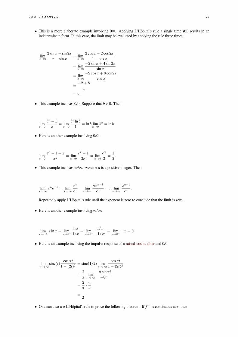
14.4. EXAMPLES 77
• This is a more elaborate example involving 0/0. Applying L'Hôpital’s rule a single time still results in anindeterminate form. In this case, the limit may be evaluated by applying the rule three times:
limx→0
2 sinx− sin 2xx− sinx = lim
x→0
2 cosx− 2 cos 2x1− cosx
= limx→0
−2 sinx+ 4 sin 2xsinx
= limx→0
−2 cosx+ 8 cos 2xcosx
=−2 + 8
1= 6.
• This example involves 0/0. Suppose that b > 0. Then
limx→0
bx − 1
x= lim
x→0
bx ln b1
= ln b limx→0
bx = ln b.
• Here is another example involving 0/0:
limx→0
ex − 1− x
x2= lim
x→0
ex − 1
2x= lim
x→0
ex
2=
1
2.
• This example involves ∞/∞. Assume n is a positive integer. Then
limx→∞
xne−x = limx→∞
xn
ex= lim
x→∞
nxn−1
ex= n lim
x→∞
xn−1
ex.
Repeatedly apply L'Hôpital’s rule until the exponent is zero to conclude that the limit is zero.
• Here is another example involving ∞/∞:
limx→0+
x lnx = limx→0+
lnx1/x
= limx→0+
1/x
−1/x2= lim
x→0+−x = 0.
• Here is an example involving the impulse response of a raised-cosine filter and 0/0:
limt→1/2
sinc(t) cosπt1− (2t)2
= sinc(1/2) limt→1/2
cosπt1− (2t)2
=2
πlim
t→1/2
−π sinπt−8t
=2
π· π4
=1
2.
• One can also use L'Hôpital’s rule to prove the following theorem. If f ′′ is continuous at x, then
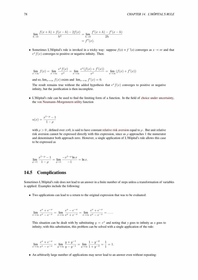
78 CHAPTER 14. L'HÔPITAL’S RULE
limh→0
f(x+ h) + f(x− h)− 2f(x)
h2= lim
h→0
f ′(x+ h)− f ′(x− h)
2h
= f ′′(x).
• Sometimes L'Hôpital’s rule is invoked in a tricky way: suppose f(x) + f ′(x) converges as x → ∞ and thatexf(x) converges to positive or negative infinity. Then:
limx→∞
f(x) = limx→∞
exf(x)
ex= lim
x→∞
ex(f(x) + f ′(x))
ex= lim
x→∞(f(x) + f ′(x))
and so, limx→∞ f(x) exists and limx→∞ f ′(x) = 0.
The result remains true without the added hypothesis that exf(x) converges to positive or negativeinfinity, but the justification is then incomplete.
• L'Hôpital’s rule can be used to find the limiting form of a function. In the field of choice under uncertainty,the von Neumann–Morgenstern utility function
u(x) =x1−ρ − 1
1− ρ
with ρ > 0 , defined over x>0, is said to have constant relative risk aversion equal to ρ . But unit relativerisk aversion cannot be expressed directly with this expression, since as ρ approaches 1 the numeratorand denominator both approach zero. However, a single application of L'Hôpital’s rule allows this caseto be expressed as
limρ→1
x1−ρ − 1
1− ρ= lim
ρ→1
−x1−ρ lnx−1
= lnx.
14.5 Complications
Sometimes L'Hôpital’s rule does not lead to an answer in a finite number of steps unless a transformation of variablesis applied. Examples include the following:
• Two applications can lead to a return to the original expression that was to be evaluated:
limx→∞
ex + e−x
ex − e−x= lim
x→∞
ex − e−x
ex + e−x= lim
x→∞
ex + e−x
ex − e−x= . . . .
This situation can be dealt with by substituting y = ex and noting that y goes to infinity as x goes toinfinity; with this substitution, this problem can be solved with a single application of the rule:
limx→∞
ex + e−x
ex − e−x= lim
y→∞
y + y−1
y − y−1= lim
y→∞
1− y−2
1 + y−2=
1
1= 1.
• An arbitrarily large number of applications may never lead to an answer even without repeating:
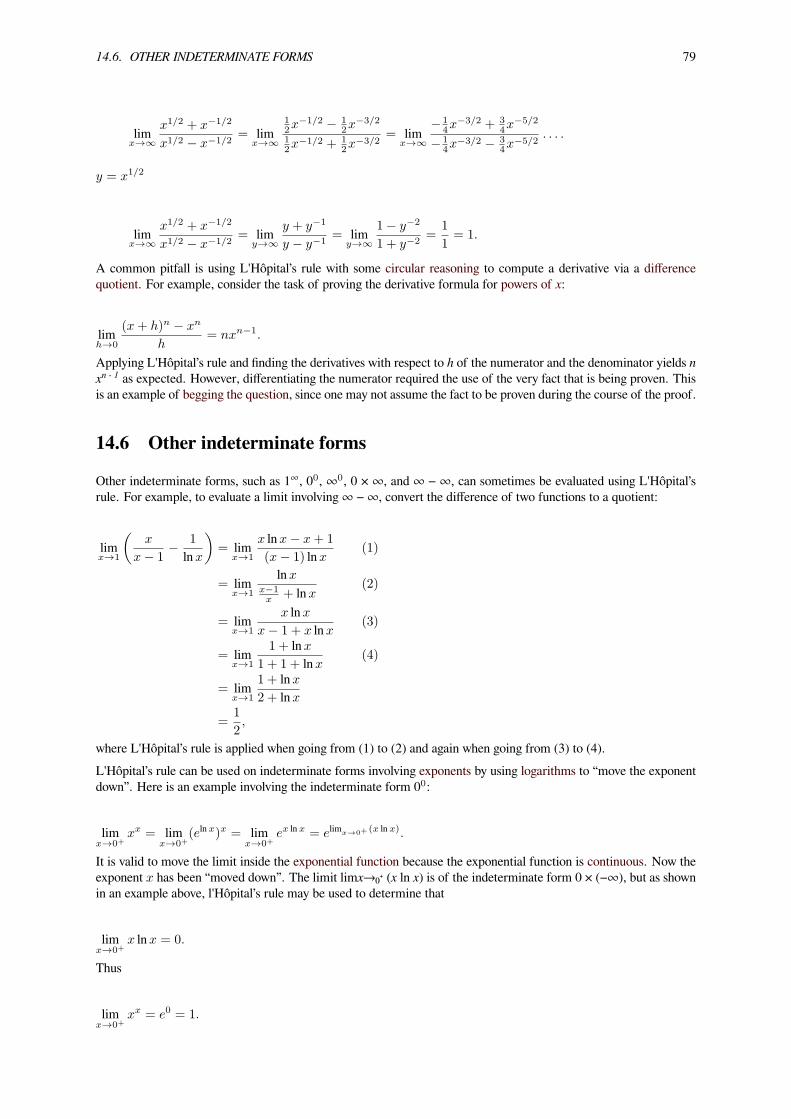
14.6. OTHER INDETERMINATE FORMS 79
limx→∞
x1/2 + x−1/2
x1/2 − x−1/2= lim
x→∞
12x
−1/2 − 12x
−3/2
12x
−1/2 + 12x
−3/2= lim
x→∞
− 14x
−3/2 + 34x
−5/2
− 14x
−3/2 − 34x
−5/2. . . .
y = x1/2
limx→∞
x1/2 + x−1/2
x1/2 − x−1/2= lim
y→∞
y + y−1
y − y−1= lim
y→∞
1− y−2
1 + y−2=
1
1= 1.
A common pitfall is using L'Hôpital’s rule with some circular reasoning to compute a derivative via a differencequotient. For example, consider the task of proving the derivative formula for powers of x:
limh→0
(x+ h)n − xn
h= nxn−1.
Applying L'Hôpital’s rule and finding the derivatives with respect to h of the numerator and the denominator yields nxn - 1 as expected. However, differentiating the numerator required the use of the very fact that is being proven. Thisis an example of begging the question, since one may not assume the fact to be proven during the course of the proof.
14.6 Other indeterminate forms
Other indeterminate forms, such as 1∞, 00, ∞0, 0 × ∞, and ∞ − ∞, can sometimes be evaluated using L'Hôpital’srule. For example, to evaluate a limit involving ∞ − ∞, convert the difference of two functions to a quotient:
limx→1
(x
x− 1− 1
lnx
)= lim
x→1
x lnx− x+ 1
(x− 1) lnx (1)
= limx→1
lnxx−1x + lnx (2)
= limx→1
x lnxx− 1 + x lnx (3)
= limx→1
1 + lnx1 + 1 + lnx (4)
= limx→1
1 + lnx2 + lnx
=1
2,
where L'Hôpital’s rule is applied when going from (1) to (2) and again when going from (3) to (4).L'Hôpital’s rule can be used on indeterminate forms involving exponents by using logarithms to “move the exponentdown”. Here is an example involving the indeterminate form 00:
limx→0+
xx = limx→0+
(eln x)x = limx→0+
ex ln x = elimx→0+ (x ln x).
It is valid to move the limit inside the exponential function because the exponential function is continuous. Now theexponent x has been “moved down”. The limit limx→₀₊ (x ln x) is of the indeterminate form 0 × (−∞), but as shownin an example above, l'Hôpital’s rule may be used to determine that
limx→0+
x lnx = 0.
Thus
limx→0+
xx = e0 = 1.

80 CHAPTER 14. L'HÔPITAL’S RULE
14.7 Other methods of evaluating limits
Although L'Hôpital’s rule is a powerful way of evaluating otherwise hard-to-evaluate limits, it is not always the easiestway. Consider
lim|x|→∞
x sin 1
x.
This limit may be evaluated using L'Hôpital’s rule:
lim|x|→∞
x sin 1
x= lim
|x|→∞
sin 1x
1/x
= lim|x|→∞
−x−2 cos 1x
−x−2
= lim|x|→∞
cos 1x
= cos(
lim|x|→∞
1
x
)= 1.
It is valid to move the limit inside the cosine function because the cosine function is continuous.But a simpler way to evaluate this limit is to use the substitution y = 1/x. As |x| approaches infinity, y approaches zero.So,
lim|x|→∞
x sin 1
x= lim
y→0
sin yy
= 1.
The final limit may be evaluated using L'Hôpital’s rule or by noting that it is the definition of the derivative of the sinefunction at zero.Still another way to evaluate this limit is to use a Taylor series expansion:
lim|x|→∞
x sin 1
x= lim
|x|→∞x
(1
x− 1
3!x3+
1
5!x5− · · ·
)= lim
|x|→∞1− 1
3!x2+
1
5!x4− · · ·
= 1 + lim|x|→∞
1
x
(− 1
3!x+
1
5!x3− · · ·
).
For |x| ≥ 1, the expression in parentheses is bounded, so the limit in the last line is zero.
14.8 Stolz–Cesàro theorem
Main article: Stolz–Cesàro theorem
The Stolz–Cesàro theorem is a similar result involving limits of sequences, but it uses finite difference operators ratherthan derivatives.
14.9 Geometric interpretation
Consider the curve in the plane whose x-coordinate is given by g(t) and whose y-coordinate is given by f(t), with bothfunctions continuous, i.e., the locus of points of the form [g(t), f(t)]. Suppose f(c) = g(c) = 0. The limit of the ratio

14.10. PROOF OF L'HÔPITAL’S RULE 81
f(t)/g(t) as t → c is the slope of the tangent to the curve at the point [g(c), f(c)] = [0, 0]. The tangent to the curve atthe point [g(t), f(t)] is given by [g′(t), f ′(t)]. L'Hôpital’s rule then states that the slope of the tangent when t = c isthe limit of the slope of the tangent to the curve as the curve approaches the origin, provided that this is defined.
14.10 Proof of L'Hôpital’s rule
14.10.1 Special case
The proof of L'Hôpital’s rule is simple in the case where f and g are continuously differentiable at the point c andwhere a finite limit is found after the first round of differentiation. It is not a proof of the general L'Hôpital’s rulebecause it is stricter in its definition, requiring both differentiability and that c be a real number. Since many commonfunctions have continuous derivatives (e.g. polynomials, sine and cosine, exponential functions), it is a special caseworthy of attention.Suppose that f and g are continuously differentiable at a real number c, that f(c) = g(c) = 0 , and that g′(c) = 0 .Then
limx→c
f(x)
g(x)= lim
x→c
f(x)− 0
g(x)− 0= lim
x→c
f(x)− f(c)
g(x)− g(c)= lim
x→c
(f(x)−f(c)
x−c
)(
g(x)−g(c)x−c
) =limx→c
(f(x)−f(c)
x−c
)limx→c
(g(x)−g(c)
x−c
) =f ′(c)
g′(c)= lim
x→c
f ′(x)
g′(x).
This follows from the difference-quotient definition of the derivative. The last equality follows from the continuity ofthe derivatives at c. The limit in the conclusion is not indeterminate because g′(c) = 0 .The proof of a more general version of L'Hôpital’s rule is given below.
14.10.2 General proof
The following proof is due to (Taylor 1952), where a unified proof for the 0/0 and ±∞/±∞ indeterminate forms isgiven. Taylor notes that different proofs may be found in (Lettenmeyer 1936) and (Wazewski 1949).Let f and g be functions satisfying the hypotheses in the General form section. Let I be the open interval in thehypothesis with endpoint c. Considering that g′(x) = 0 on this interval and g is continuous, I can be chosen smallerso that g is nonzero on I .[8]
For each x in the interval, definem(x) = inf f ′(ξ)g′(ξ) andM(x) = sup f ′(ξ)
g′(ξ) as ξ ranges over all values between x andc. (The symbols inf and sup denote the infimum and supremum.)From the differentiability of f and g on I , Cauchy’s mean value theorem ensures that for any two distinct points x andy in I there exists a ξ between x and y such that f(x)−f(y)
g(x)−g(y) = f ′(ξ)g′(ξ) . Consequentlym(x) ≤ f(x)−f(y)
g(x)−g(y) ≤M(x) forall choices of distinct x and y in the interval. The value g(x)-g(y) is always nonzero for distinct x and y in the interval,for if it was not, the mean value theorem would imply the existence of a p between x and y such that g' (p)=0.The definition of m(x) and M(x) will result in an extended real number, and so it is possible for them to take on thevalues ±∞. In the following two cases, m(x) and M(x) will establish bounds on the ratio f/g.Case 1: limx→c f(x) = limx→c g(x) = 0
For any x in the interval I , and point y between x and c,
m(x) ≤ f(x)− f(y)
g(x)− g(y)=
f(x)g(x) −
f(y)g(x)
1− g(y)g(x)
≤M(x)
and therefore as y approaches c, f(y)g(x) and
g(y)g(x) become zero, and so
m(x) ≤ f(x)
g(x)≤M(x)
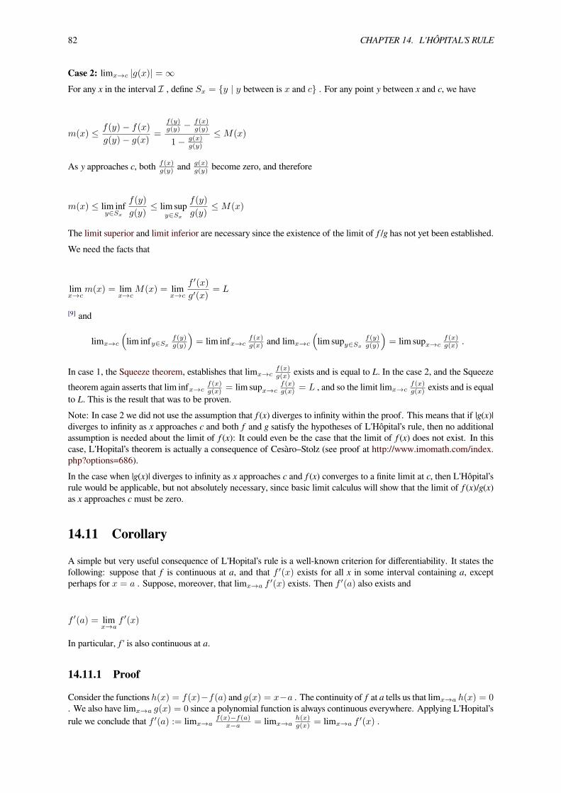
82 CHAPTER 14. L'HÔPITAL’S RULE
Case 2: limx→c |g(x)| = ∞For any x in the interval I , define Sx = y | y between is x and c . For any point y between x and c, we have
m(x) ≤ f(y)− f(x)
g(y)− g(x)=
f(y)g(y) −
f(x)g(y)
1− g(x)g(y)
≤M(x)
As y approaches c, both f(x)g(y) and
g(x)g(y) become zero, and therefore
m(x) ≤ lim infy∈Sx
f(y)
g(y)≤ lim sup
y∈Sx
f(y)
g(y)≤M(x)
The limit superior and limit inferior are necessary since the existence of the limit of f/g has not yet been established.We need the facts that
limx→c
m(x) = limx→c
M(x) = limx→c
f ′(x)
g′(x)= L
[9] and
limx→c
(lim infy∈Sx
f(y)g(y)
)= lim infx→c
f(x)g(x) and limx→c
(lim supy∈Sx
f(y)g(y)
)= lim supx→c
f(x)g(x) .
In case 1, the Squeeze theorem, establishes that limx→cf(x)g(x) exists and is equal to L. In the case 2, and the Squeeze
theorem again asserts that lim infx→cf(x)g(x) = lim supx→c
f(x)g(x) = L , and so the limit limx→c
f(x)g(x) exists and is equal
to L. This is the result that was to be proven.Note: In case 2 we did not use the assumption that f(x) diverges to infinity within the proof. This means that if |g(x)|diverges to infinity as x approaches c and both f and g satisfy the hypotheses of L'Hôpital’s rule, then no additionalassumption is needed about the limit of f(x): It could even be the case that the limit of f(x) does not exist. In thiscase, L'Hopital’s theorem is actually a consequence of Cesàro–Stolz (see proof at http://www.imomath.com/index.php?options=686).In the case when |g(x)| diverges to infinity as x approaches c and f(x) converges to a finite limit at c, then L'Hôpital’srule would be applicable, but not absolutely necessary, since basic limit calculus will show that the limit of f(x)/g(x)as x approaches c must be zero.
14.11 Corollary
A simple but very useful consequence of L'Hopital’s rule is a well-known criterion for differentiability. It states thefollowing: suppose that f is continuous at a, and that f ′(x) exists for all x in some interval containing a, exceptperhaps for x = a . Suppose, moreover, that limx→a f
′(x) exists. Then f ′(a) also exists and
f ′(a) = limx→a
f ′(x)
In particular, f' is also continuous at a.
14.11.1 Proof
Consider the functions h(x) = f(x)−f(a) and g(x) = x−a . The continuity of f at a tells us that limx→a h(x) = 0. We also have limx→a g(x) = 0 since a polynomial function is always continuous everywhere. Applying L'Hopital’srule we conclude that f ′(a) := limx→a
f(x)−f(a)x−a = limx→a
h(x)g(x) = limx→a f
′(x) .

14.12. SEE ALSO 83
14.12 See also
• L'Hôpital controversy
14.13 Notes[1] In the 17th and 18th centuries, the name was commonly spelled “l'Hospital”, and he himself spelled his name that way.
However, French spellings have been altered: the silent 's’ has been removed and replaced with the circumflex over thepreceding vowel. The former spelling is still used in English where there is no circumflex.
[2] O'Connor, John J.; Robertson, Edmund F. “De L'Hopital biography”. The MacTutor History of Mathematics archive.Scotland: School of Mathematics and Statistics, University of St Andrews. Retrieved 21 December 2008.
[3] L’Hospital, Analyse des infiniment petits... , pages 145–146: “Proposition I. Problême. Soit une ligne courbe AMD (AP =x, PM = y, AB = a [see Figure 130] ) telle que la valeur de l’appliquée y soit exprimée par une fraction, dont le numérateur& le dénominateur deviennent chacun zero lorsque x = a, c’est à dire lorsque le point P tombe sur le point donné B. Ondemande quelle doit être alors la valeur de l’appliquée BD. [Solution: ]...si l’on prend la difference du numérateur, & qu’onla divise par la difference du denominateur, apres avoir fait x = a = Ab ou AB, l’on aura la valeur cherchée de l’appliquéebd ou BD.” Translation : “Let there be a curve AMD (where AP = X, PM = y, AB = a) such that the value of the ordinatey is expressed by a fraction whose numerator and denominator each become zero when x = a; that is, when the point P fallson the given point B. One asks what shall then be the value of the ordinate BD. [Solution: ]... if one takes the differentialof the numerator and if one divides it by the differential of the denominator, after having set x = a = Ab or AB, one willhave the value [that was] sought of the ordinate bd or BD.”
[4] Weisstein, Eric W., “L'Hospital’s Rule”, MathWorld.
[5] (Chatterjee 2005, p. 291)
[6] The functional analysis definition of the limit of a function does not require the existence of this connected interval.
[7] (Krantz 2004, p.79)
[8] Since g' is nonzero and g is continuous on the interval, it is impossible for g to be zero more than once on the interval. Ifit had two zeros, the mean value theorem would assert the existence of a point p in the interval between the zeros such thatg' (p)=0. So either g is already nonzero on the interval, or else the interval can be reduced in size so as not to contain thesingle zero of g.
[9] Note limx→c m(x) and limx→c M(x) exist as they are nondecreasing and nonincreasing functions of x, respectively.Consider a sequence xi → c , we easily have limi m(xi) ⩽ limi
f ′(xi)g′(xi)
⩽ limi M(xi) , as the inequality holds for eachi; this yields the inequalities limx→c m(x) ⩽ limx→c
f ′(x)g′(x) ⩽ limx→c M(x)We show limx→c M(x) ⩽ limx→c
f ′(x)g′(x) .
Indeed, fix a sequence of numbers ϵi > 0 such that limi ϵi = 0 , and a sequence xi → c . For each i, we may choose xi <
yi < c such that f ′(yi)g′(yi)
+ ϵi ⩾ supxi<ξ<cf ′(ξ)g′(ξ) , by the definition of sup . Thus we have limi M(xi) ⩽ limi
f ′(yi)g′(yi)
+ ϵi
= limif ′(yi)g′(yi)
+ limi ϵi = limif ′(yi)g′(yi)
as desired. The argument that limx→c m(x) ⩾ limx→cf ′(x)g′(x) is similar.
14.14 References
• Chatterjee, Dipak (2005), Real Analysis, PHI Learning Pvt. Ltd, ISBN 81-203-2678-4
• Krantz, Steven G. (2004), A handbook of real variables. With applications to differential equations and Fourieranalysis, Boston, MA: Birkhäuser Boston Inc., pp. xiv+201, ISBN 0-8176-4329-X, MR 2015447
• Lettenmeyer, F. (1936), "Über die sogenannte Hospitalsche Regel”, Journal für die reine und angewandteMathematik 174: 246–247, doi:10.1515/crll.1936.174.246
• Taylor, A. E. (1952), “L'Hospital’s rule”, Amer. Math. Monthly 59: 20–24, doi:10.2307/2307183, ISSN0002-9890, MR 0044602
• Wazewski, T. (1949), “Quelques démonstrations uniformes pour tous les cas du théorème de l'Hôpital. Général-isations”, Prace Mat.-Fiz. (in French) 47: 117–128, MR 0034430
84 CHAPTER 14. L'HÔPITAL’S RULE
14.15 External links• L'Hôpital’s rule at imomath.com
• Kudryavtsev, L.D. (2001), “L'Hospital rule”, in Hazewinkel, Michiel, Encyclopedia of Mathematics, Springer,ISBN 978-1-55608-010-4
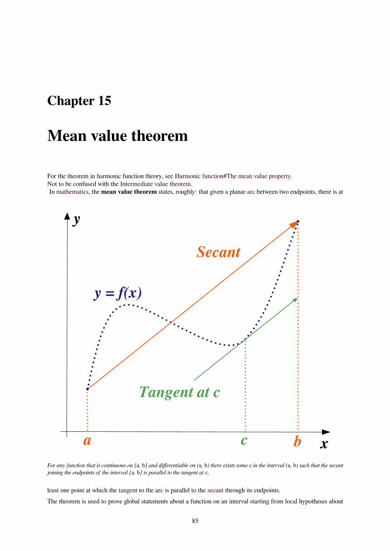
Chapter 15
Mean value theorem
For the theorem in harmonic function theory, see Harmonic function#The mean value property.Not to be confused with the Intermediate value theorem.In mathematics, themean value theorem states, roughly: that given a planar arc between two endpoints, there is at
Secant
Tangent at c
y = f(x)
a bc x
y
For any function that is continuous on [a, b] and differentiable on (a, b) there exists some c in the interval (a, b) such that the secantjoining the endpoints of the interval [a, b] is parallel to the tangent at c.
least one point at which the tangent to the arc is parallel to the secant through its endpoints.The theorem is used to prove global statements about a function on an interval starting from local hypotheses about
85

86 CHAPTER 15. MEAN VALUE THEOREM
derivatives at points of the interval.More precisely, if a function f is continuous on the closed interval [a, b], where a < b, and differentiable on the openinterval (a, b), then there exists a point c in (a, b) such that
f ′(c) = f(b)−f(a)b−a . [1]
A special case of this theorem was first described by Parameshvara (1370–1460) from the Kerala school of as-tronomy and mathematics in his commentaries on Govindasvāmi and Bhaskara II.[2] The mean value theorem inits modern form was later stated by Augustin Louis Cauchy (1789–1857). It is one of the most important resultsin differential calculus, as well as one of the most important theorems in mathematical analysis, and is useful inproving the fundamental theorem of calculus. The mean value theorem follows from the more specific statement ofRolle’s theorem, and can be used to prove the more general statement of Taylor’s theorem (with Lagrange form ofthe remainder term).
15.1 Formal statement
Let f : [a, b] → R be a continuous function on the closed interval [a, b], and differentiable on the open interval (a,b), where a < b. Then there exists some c in (a, b) such that
f ′(c) =f(b)− f(a)
b− a.
The mean value theorem is a generalization of Rolle’s theorem, which assumes f(a) = f(b), so that the right-handside above is zero.The mean value theorem is still valid in a slightly more general setting. One only needs to assume that f : [a, b] → Ris continuous on [a, b], and that for every x in (a, b) the limit
limh→0
f(x+ h)− f(x)
h
exists as a finite number or equals +∞ or −∞. If finite, that limit equals f′ (x). An example where this version of thetheorem applies is given by the real-valued cube root function mapping x to x1/3, whose derivative tends to infinity atthe origin.Note that the theorem, as stated, is false if a differentiable function is complex-valued instead of real-valued. Forexample, define f(x) = eix for all real x. Then
f(2π) − f(0) = 0 = 0(2π − 0)
while f′ (x) ≠ 0 for any real x.
15.2 Proof
The expression (f(b) − f(a)) / (b − a) gives the slope of the line joining the points (a, f(a)) and (b, f(b)), which is achord of the graph of f, while f '(x) gives the slope of the tangent to the curve at the point (x, f(x)). Thus the Meanvalue theorem says that given any chord of a smooth curve, we can find a point lying between the end-points of thechord such that the tangent at that point is parallel to the chord. The following proof illustrates this idea.Define g(x) = f(x) − rx, where r is a constant. Since f is continuous on [a, b] and differentiable on (a, b), the same istrue for g. We now want to choose r so that g satisfies the conditions of Rolle’s theorem. Namely

15.3. A SIMPLE APPLICATION 87
g(a) = g(b) ⇐⇒ f(a)− ra = f(b)− rb
⇐⇒ r(b− a) = f(b)− f(a)
⇐⇒ r =f(b)− f(a)
b− a·
By Rolle’s theorem, since g is differentiable and g(a) = g(b), there is some c in (a, b) for which g′ (c) = 0, and it followsfrom the equality g(x) = f(x) − rx that,
f ′(c) = g′(c) + r = 0 + r =f(b)− f(a)
b− a
as required.
15.3 A simple application
Assume that f is a continuous, real-valued function, defined on an arbitrary interval I of the real line. If the derivativeof f at every interior point of the interval I exists and is zero, then f is constant.Proof: Assume the derivative of f at every interior point of the interval I exists and is zero. Let (a, b) be an arbitraryopen interval in I. By the mean value theorem, there exists a point c in (a,b) such that
0 = f ′(c) =f(b)− f(a)
b− a.
This implies that f(a) = f(b). Thus, f is constant on the interior of I and thus is constant on I by continuity. (Seebelow for a multivariable version of this result.)Remarks:
• Only continuity of f, not differentiability, is needed at the endpoints of the interval I. No hypothesis of continuityneeds to be stated if I is an open interval, since the existence of a derivative at a point implies the continuity atthis point. (See the section continuity and differentiability of the article derivative.)
• The differentiability of f can be relaxed to one-sided differentiability, a proof given in the article on semi-differentiability.
15.4 Cauchy’s mean value theorem
Cauchy’s mean value theorem, also known as the extended mean value theorem, is a generalization of the meanvalue theorem. It states: If functions f and g are both continuous on the closed interval [a,b], and differentiable onthe open interval (a, b), then there exists some c ∈ (a,b), such that
(f(b)− f(a))g ′(c) = (g(b)− g(a))f ′(c).
Of course, if g(a) ≠ g(b) and if g′(c) ≠ 0, this is equivalent to:
f ′(c)
g′(c)=f(b)− f(a)
g(b)− g(a)·
Geometrically, this means that there is some tangent to the graph of the curve
[a, b] −→ R2
t 7→(f(t), g(t)
),

88 CHAPTER 15. MEAN VALUE THEOREM
Geometrical meaning of Cauchy’s theorem
which is parallel to the line defined by the points (f(a),g(a)) and (f(b),g(b)). However Cauchy’s theorem does notclaim the existence of such a tangent in all cases where (f(a),g(a)) and (f(b),g(b)) are distinct points, since it mightbe satisfied only for some value c with f′(c) = g′(c) = 0, in other words a value for which the mentioned curve isstationary; in such points no tangent to the curve is likely to be defined at all. An example of this situation is the curvegiven by
t 7→ (t3, 1− t2),
which on the interval [−1,1] goes from the point (−1,0) to (1,0), yet never has a horizontal tangent; however it has astationary point (in fact a cusp) at t = 0.Cauchy’s mean value theorem can be used to prove l'Hôpital’s rule. The mean value theorem is the special case ofCauchy’s mean value theorem when g(t) = t.
15.4.1 Proof of Cauchy’s mean value theorem
The proof of Cauchy’s mean value theorem is based on the same idea as the proof of the mean value theorem.
• Suppose that g(a) ≠ g(b). Define h(x) = f(x) − rg(x), where r is fixed in such a way that h(a) = h(b), namely
15.5. GENERALIZATION FOR DETERMINANTS 89
h(a) = h(b) ⇐⇒ f(a)− r g(a) = f(b)− r g(b)
⇐⇒ r (g(b)− g(a)) = f(b)− f(a)
⇐⇒ r =f(b)− f(a)
g(b)− g(a).
Since f and g are continuous on [a, b] and differentiable on (a, b), the same is true for h. All in all, hsatisfies the conditions of Rolle’s theorem: consequently, there is some c in (a, b) for which h′ (c) = 0.From the equality h(x) = f(x) − rg(x) it follows that,
0 = h′(c) = f ′(c)− r g′(c) ⇒ (g(b)− g(a)) f ′(c) = (g(b)− g(a)) r g′(c) = (f(b)− f(a)) g′(c)
as required.
• If instead g(a) = g(b), then, applying Rolle’s theorem to g, it follows that there exists c in (a, b) for which g′ (c)= 0. Using this choice of c, Cauchy’s mean value theorem (trivially) holds.
15.5 Generalization for determinants
Assume that f , g , and h are differentiable functions on (a, b) that are continuous on [a, b] . Define
D(x) =
∣∣∣∣∣∣f(x) g(x) h(x)f(a) g(a) h(a)f(b) g(b) h(b)
∣∣∣∣∣∣There exists c ∈ (a, b) such that D′(c) = 0 .Notice that
D′(x) =
∣∣∣∣∣∣f ′(x) g′(x) h′(x)f(a) g(a) h(a)f(b) g(b) h(b)
∣∣∣∣∣∣and if we place h(x) = 1 , we get Cauchy’s mean value theorem. If we place h(x) = 1 and g(x) = x we getLagrange’s mean value theorem.The proof of the generalization is quite simple: each of D(a) and D(b) are determinants with two identical rows,hence D(a) = D(b) = 0 . The Rolle’s theorem implies that there exists c ∈ (a, b) such that D′(c) = 0 .
15.6 Mean value theorem in several variables
The mean value theorem generalizes to real functions of multiple variables. The trick is to use parametrization tocreate a real function of one variable, and then apply the one-variable theorem.Let G be an open connected subset of Rn, and let f : G → R be a differentiable function. Fix points x, y ∈ G suchthat the interval x y lies in G, and define g(t) = f((1 − t)x + ty). Since g is a differentiable function in one variable, themean value theorem gives:
g(1)− g(0) = g′(c)
for some c between 0 and 1. But since g(1) = f(y) and g(0) = f(x), computing g′ (c) explicitly we have:
f(y)− f(x) = ∇f((1− c)x+ cy) · (y − x)

90 CHAPTER 15. MEAN VALUE THEOREM
where ∇ denotes a gradient and · a dot product. Note that this is an exact analog of the theorem in one variable (inthe case n = 1 this is the theorem in one variable). By the Schwarz inequality, the equation gives the estimate:
|f(y)− f(x)| ≤ |∇f((1− c)x+ cy)| |y − x|.
In particular, when the partial derivatives of f are bounded, f is Lipschitz continuous (and therefore uniformly con-tinuous). Note that f is not assumed to be continuously differentiable nor continuous on the closure of G. However,in the above, we used the chain rule so the existence of ∇f would not be sufficient.As an application of the above, we prove that f is constant if G is open and connected and every partial derivative off is 0. Pick some point x0 ∈ G, and let g(x) = f(x) − f(x0). We want to show g(x) = 0 for every x ∈ G. For that, let E= x ∈ G : g(x) = 0 . Then E is closed and nonempty. It is open too: for every x ∈ E,
|g(y)| = |g(y)− g(x)| ≤ (0)|y − x| = 0
for every y in some neighborhood of x. (Here, it is crucial that x and y are sufficiently close to each other.) Since Gis connected, we conclude E = G.Remark that all arguments in the above are made in a coordinate-free manner; hence, they actually generalize to thecase when G is a subset of a Banach space.
15.7 Mean value theorem for vector-valued functions
There is no exact analog of the mean value theorem for vector-valued functions.Jean Dieudonné in his classic treatise Foundations of Modern Analysis discards the mean value theorem and replacesit by mean inequality as the proof is not constructive and by no way one can find the mean value. In applications oneonly needs mean inequality. Serge Lang in Analysis I uses the mean value theorem, in integral form, as an instantreflex but this use requires the continuity of the derivative. If one uses the Henstock-Kurzweil integral one can havethe mean value theorem in integral form without the additional assumption that derivative should be continuous asevery derivative is Henstock-Kurzweil integrable. The problem is roughly speaking the following: If f : U → Rm isa differentiable function (where U ⊂ Rn is open) and if x + th, x, h ∈ Rn, t ∈ [0, 1] is the line segment in question(lying inside U), then one can apply the above parametrization procedure to each of the component functions fi (i =1, ..., m) of f (in the above notation set y = x + h). In doing so one finds points x + tih on the line segment satisfying
fi(x+ h)− fi(x) = ∇fi(x+ tih) · h.
But generally there will not be a single point x + t*h on the line segment satisfying
fi(x+ h)− fi(x) = ∇fi(x+ t∗h) · h.
for all i simultaneously. (As a counterexample one could take f : [0, 2π] → R2 defined via the component functionsf1(x) = cos(x), f2(x) = sin(x). Then f(2π) − f(0) = 0 ∈ R2, but f ′1(x) = − sin(x) and f ′2(x) = cos(x) are neversimultaneously zero as x ranges over [0, 2π].)However a certain type of generalization of the mean value theorem to vector-valued functions is obtained as follows:Let f be a continuously differentiable real-valued function defined on an open interval I, and let x as well as x + h bepoints of I. The mean value theorem in one variable tells us that there exists some t* between 0 and 1 such that
f(x+ h)− f(x) = f ′(x+ t∗h) · h.
On the other hand, we have, by the fundamental theorem of calculus followed by a change of variables,
f(x+ h)− f(x) =
∫ x+h
x
f ′(u)du =
(∫ 1
0
f ′(x+ th) dt
)· h.
15.7. MEAN VALUE THEOREM FOR VECTOR-VALUED FUNCTIONS 91
Thus, the value f′ (x + t*h) at the particular point t* has been replaced by the mean value
∫ 1
0
f ′(x+ th) dt.
This last version can be generalized to vector valued functions:Let U ⊂ Rn be open, f : U → Rm continuously differentiable, and x ∈ U, h ∈ Rn vectors such that the whole linesegment x + th, 0 ≤ t ≤ 1 remains in U. Then we have:
(*) f(x+ h)− f(x) =
(∫ 1
0
Df(x+ th) dt
)· h,
where the integral of a matrix is to be understood componentwise. (Df denotes the Jacobian matrix of f.)From this one can further deduce that if ||Df(x + th)|| is bounded for t between 0 and 1 by some constant M, then
(**) ∥f(x+ h)− f(x)∥ ≤M∥h∥.
Proof of (*). Write fi (i = 1, ..., m) for the real valued components of f. Define the functions gi: [0, 1] → R by gi(t):= fi(x + th).Then we have
fi(x+h)−fi(x) = gi(1)−gi(0) =∫ 1
0
g′i(t)dt =
∫ 1
0
n∑j=1
∂fi∂xj
(x+ th)hj
dt =n∑
j=1
(∫ 1
0
∂fi∂xj
(x+ th) dt
)hj .
The claim follows since Df is the matrix consisting of the components ∂fi∂xj
, q.e.d.Proof of (**). From (*) it follows that
∥f(x+ h)− f(x)∥ =
∥∥∥∥∫ 1
0
(Df(x+ th) · h) dt∥∥∥∥ ≤
∫ 1
0
∥Df(x+ th)∥ · ∥h∥ dt ≤M∥h∥.
Here we have used the followingLemma. Let v : [a, b] → Rm be a continuous function defined on the interval [a, b] ⊂ R. Then we have
(***)∥∥∥∫ b
av(t) dt
∥∥∥ ≤∫ b
a∥v(t)∥ dt.
Proof of (***). Let u in Rm denote the value of the integral
u :=
∫ b
a
v(t) dt.
Now
∥u∥2 = ⟨u, u⟩ =
⟨∫ b
a
v(t)dt, u
⟩=
∫ b
a
⟨v(t), u⟩ dt ≤∫ b
a
∥v(t)∥ · ∥u∥ dt = ∥u∥∫ b
a
∥v(t)∥ dt,
thus ∥u∥ ≤∫ b
a∥v(t)∥ dt as desired. (Note the use of the Cauchy–Schwarz inequality.) This shows (***) and thereby
finishes the proof of (**).

92 CHAPTER 15. MEAN VALUE THEOREM
15.8 Mean Value Theorems for Definite Integrals
15.8.1 First Mean Value Theorem for Definite Integrals
Let f : [a, b] → R be a continuous function. Then there exists c in (a, b) such that
∫ b
a
f(x) dx = f(c)(b− a).
Since the mean value of f on [a, b] is defined as
1
b− a
∫ b
a
f(x) dx,
we can interpret the conclusion as f achieves its mean value at some c in (a, b).[3]
In general, if f : [a, b] → R is continuous and g is an integrable function that does not change sign on [a, b], thenthere exists c in (a, b) such that
∫ b
a
f(x)g(x) dx = f(c)
∫ b
a
g(x) dx.
15.8.2 Proof of the First Mean Value Theorem for Definite Integrals
Suppose f : [a, b] → R is continuous and g is a nonnegative integrable function on [a, b]. By the extreme valuetheorem, there exists m and M such that for each x in [a, b],m ≤ f(x) ≤M. Since g is nonnegative,
m
∫ b
a
g(x) dx ≤∫ b
a
f(x)g(x) dx ≤M
∫ b
a
g(x) dx.
Now let I =∫ b
ag(x) dx. If I = 0 , we're done since 0 ≤
∫ b
af(x)g(x) dx ≤ 0 means
∫ b
af(x)g(x) dx = 0, so for
any c in (a, b),
∫ b
a
f(x)g(x) dx = f(c) I = 0.
If I ≠ 0, thenm ≤ 1I
∫ b
af(x)g(x) dx ≤M. By the intermediate value theorem, f attains every value of the interval
[m, M], so for some c in [a, b]
f(c) =1
I
∫ b
a
f(x)g(x) dx,
that is,
15.8. MEAN VALUE THEOREMS FOR DEFINITE INTEGRALS 93
∫ b
a
f(x)g(x) dx = f(c)
∫ b
a
g(x) dx.
Finally, if g is negative on [a, b], then
M
∫ b
a
g(x) dx ≤∫ b
a
f(x)g(x) dx ≤ m
∫ b
a
g(x) dx,
and we still get the same result as above.QED
15.8.3 Second Mean Value Theorem for Definite Integrals
There are various slightly different theorems called the second mean value theorem for definite integrals. Acommonly found version is as follows:
If G : [a, b] → R is a positive monotonically decreasing function and φ : [a, b] → R is an integrablefunction, then there exists a number x in (a, b] such that
∫ b
a
G(t)φ(t) dt = G(a+)
∫ x
a
φ(t) dt.
Here G(a+) stands for limx→a+ G(x) , the existence of which follows from the conditions. Note that it is essentialthat the interval (a, b] contains b. A variant not having this requirement is:[4]
If G : [a, b] → R is a monotonic (not necessarily decreasing and positive) function and φ : [a, b] → Ris an integrable function, then there exists a number x in (a, b) such that
∫ b
a
G(t)φ(t) dt = G(a+)
∫ x
a
φ(t) dt+G(b−)
∫ b
x
φ(t) dt.
15.8.4 Mean value theorem for integration fails for vector-valued functions
If the function G returns a multi-dimensional vector, then the MVT for integration is not true, even if the domain ofG is also multi-dimensional.For example, consider the following 2-dimensional function defined on an n -dimensional cube:
G : [0, 2π]n → R2
G(x1, · · · , xn) = (sin(x1 + · · ·+ xn), cos(x1 + · · ·+ xn))
Then, by symmetry it is easy to see that the mean value of G over its domain is (0,0):
∫[0,2π]n
G(x1, · · · , xn)dx1 · · · dxn = (0, 0)
However, there is no point in which G = (0, 0) , because |G| = 1 everywhere.

94 CHAPTER 15. MEAN VALUE THEOREM
15.9 A probabilistic analogue of the mean value theorem
Let X and Y be non-negative random variables such that E[X] < E[Y] < ∞ and X ≤st Y (i.e. X is smaller thanY in the usual stochastic order). Then there exists an absolutely continuous non-negative random variable Z havingprobability density function
fZ(x) =Pr(Y > x)− Pr(X > x)
E[Y ]− E[X], x ≥ 0.
Let g be ameasurable and differentiable function such that E[g(X)], E[g(Y)] <∞, and let its derivative g′ bemeasurableand Riemann-integrable on the interval [x, y] for all y ≥ x ≥ 0. Then, E[g′ (Z)] is finite and[5]
E[g(Y )]− E[g(X)] = E[g′(Z)] [E(Y )− E(X)].
15.10 Generalization in complex analysis
As noted above, the theorem does not hold for differentiable complex-valued functions. Instead, a generalization ofthe theorem is stated such:[6]
Let f : Ω → C be a holomorphic function on the open convex set Ω, and let a and b be distinct points in Ω. Thenthere exist points u, v on Lab (the line segment from a to b) such that
Re(f ′(u)) = Re(f(b)− f(a)
b− a
),
Im(f ′(v)) = Im(f(b)− f(a)
b− a
).
Where Re() is the Real part and Im() is the Imaginary part of a complex-valued function.
15.11 See also• Newmark-beta method
• Mean value theorem (divided differences)
15.12 Notes[1] Weisstein, Eric. “Mean-Value Theorem”. MathWorld. Wolfram Research. Retrieved 24 March 2011.
[2] J. J. O'Connor and E. F. Robertson (2000). Paramesvara, MacTutor History of Mathematics archive.
[3] Michael Comenetz (2002). Calculus: The Elements. World Scientific. p. 159. ISBN 978-981-02-4904-5.
[4] E. W. Hobson (1909). On the Second Mean-Value Theorem of the Integral Calculus. Proc. London Math Soc. S2-7, no.1, pp.14-23. MR1575669. Available online: .
[5] A. Di Crescenzo (1999). A probabilistic analogue of the mean value theorem and its applications to reliability theory. J.Appl. Prob. 36, 706-719.
[6] “Complex Mean-Value Theorem”. PlanetMath. PlanetMath.

15.13. EXTERNAL LINKS 95
15.13 External links• Hazewinkel, Michiel, ed. (2001), “Cauchy theorem”, Encyclopedia of Mathematics, Springer, ISBN 978-1-55608-010-4
• PlanetMath: Mean-Value Theorem
• Weisstein, Eric W., “Mean value theorem”, MathWorld.
• Weisstein, Eric W., “Cauchy’s Mean-Value Theorem”, MathWorld.
• “Mean Value Theorem: Intuition behind the Mean Value Theorem” at the Khan Academy

Chapter 16
Monotone convergence theorem
In the mathematical field of real analysis, themonotone convergence theorem is any of a number of related theoremsproving the convergence of monotonic sequences (sequences that are increasing or decreasing) that are also bounded.Informally, the theorems state that if a sequence is increasing and bounded above by a supremum, then the sequencewill converge to the supremum; in the same way, if a sequence is decreasing and is bounded below by an infimum, itwill converge to the infimum.
16.1 Convergence of a monotone sequence of real numbers
16.1.1 Lemma 1
If a sequence of real numbers is increasing and bounded above, then its supremum is the limit.
16.1.2 Proof
We prove that if an increasing sequence an is bounded above, then it is convergent and the limit is supnan .
Since an is non-empty and by assumption, it is bounded above, then, by the Least upper bound property of realnumbers, c = supnan exists and is finite. Now for every ε > 0 , there exists N such that aN > c − ε , sinceotherwise c− ε is an upper bound of an , which contradicts to c being supnan . Then since an is increasing,if n > N, |c− an| ≤ |c− aN | < ε , hence by definition, the limit of an is supnan.
16.1.3 Lemma 2
If a sequence of real numbers is decreasing and bounded below, then its infimum is the limit.
16.1.4 Proof
The proof is similar to the proof for the case when the sequence is increasing and bounded above.
16.1.5 Theorem
If an is a monotone sequence of real numbers (i.e., if an ≤ an₊₁ for every n ≥ 1 or an ≥ an₊₁ for every n ≥ 1), thenthis sequence has a finite limit if and only if the sequence is bounded.[1]
16.1.6 Proof
The proof follows directly from the lemmas.
96
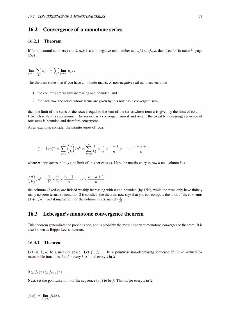
16.2. CONVERGENCE OF A MONOTONE SERIES 97
16.2 Convergence of a monotone series
16.2.1 Theorem
If for all natural numbers j and k, aj,k is a non-negative real number and aj,k ≤ aj₊₁,k, then (see for instance [2] page168)
limj→∞
∑k
aj,k =∑k
limj→∞
aj,k.
The theorem states that if you have an infinite matrix of non-negative real numbers such that
1. the columns are weakly increasing and bounded, and
2. for each row, the series whose terms are given by this row has a convergent sum,
then the limit of the sums of the rows is equal to the sum of the series whose term k is given by the limit of columnk (which is also its supremum). The series has a convergent sum if and only if the (weakly increasing) sequence ofrow sums is bounded and therefore convergent.As an example, consider the infinite series of rows
(1 + 1/n)n =n∑
k=0
(n
k
)/nk =
n∑k=0
1
k!× n
n× n− 1
n× · · · × n− k + 1
n,
where n approaches infinity (the limit of this series is e). Here the matrix entry in row n and column k is
(n
k
)/nk =
1
k!× n
n× n− 1
n× · · · × n− k + 1
n;
the columns (fixed k) are indeed weakly increasing with n and bounded (by 1/k!), while the rows only have finitelymany nonzero terms, so condition 2 is satisfied; the theorem now says that you can compute the limit of the row sums(1 + 1/n)n by taking the sum of the column limits, namely 1
k! .
16.3 Lebesgue’s monotone convergence theorem
This theorem generalizes the previous one, and is probably the most important monotone convergence theorem. It isalso known as Beppo Levi's theorem.
16.3.1 Theorem
Let (X, Σ, μ) be a measure space. Let f1, f2, . . . be a pointwise non-decreasing sequence of [0, ∞]-valued Σ–measurable functions, i.e. for every k ≥ 1 and every x in X,
0 ≤ fk(x) ≤ fk+1(x).
Next, set the pointwise limit of the sequence (fn) to be f. That is, for every x in X,
f(x) := limk→∞
fk(x).
98 CHAPTER 16. MONOTONE CONVERGENCE THEOREM
Then f is Σ–measurable and
limk→∞
∫fk dµ =
∫f dµ.
Remark. If the sequence (fk) satisfies the assumptions μ–almost everywhere, one can find a set N ∈ Σ with μ(N) =0 such that the sequence (fk(x)) is non-decreasing for every x /∈ N . The result remains true because for every k,
∫fk dµ =
∫X\N
fk dµ, and∫f dµ =
∫X\N
f dµ,
provided that f is Σ–measurable (see for instance [3] section 21.38).
16.3.2 Proof
We will first show that f is Σ–measurable (see for instance [3] section 21.3). To do this, it is sufficient to show thatthe inverse image of an interval [0, t] under f is an element of the sigma algebra Σ on X, because (closed) intervalsgenerate the Borel sigma algebra on the reals. Let I = [0, t] be such a subinterval of [0, ∞]. Let
f−1(I) = x ∈ X | f(x) ∈ I.
Since I is a closed interval and ∀k, fk(x) ≤ f(x) ,
f(x) ∈ I ⇔ fk(x) ∈ I, ∀k ∈ N.
Thus,
x ∈ X | f(x) ∈ I =∩k∈N
x ∈ X | fk(x) ∈ I.
Note that each set in the countable intersection is an element of Σ because it is the inverse image of a Borel subsetunder a Σ-measurable function fk . Since sigma algebras are, by definition, closed under countable intersections,this shows that f is Σ-measurable. In general, the supremum of any countable family of measurable functions is alsomeasurable.Now we will prove the rest of the monotone convergence theorem. The fact that f is Σ-measurable implies that theexpression
∫f dµ is well defined.
We will start by showing that∫f dµ ≥ limk
∫fk dµ.
By the definition of the Lebesgue integral,
∫f dµ = sup
∫g dµ | g ∈ SF, g ≤ f
,
where SF is the set of Σ-measurable simple functions on X. Since fk(x) ≤ f(x) at every x ∈ X, we have that
∫g dµ | g ∈ SF, g ≤ fk
⊆∫
g dµ | g ∈ SF, g ≤ f
.
Hence, since the supremum of a subset cannot be larger than that of the whole set, we have that:
∫f dµ ≥ lim
k
∫fk dµ,
16.3. LEBESGUE’S MONOTONE CONVERGENCE THEOREM 99
and the limit on the right exists, since the sequence is monotonic.We now prove the inequality in the other direction (which also follows from Fatou’s lemma), that is we seek to showthat
∫f dµ ≤ lim
k
∫fk dµ.
It follows from the definition of integral, that there is a non-decreasing sequence (gk) of non-negative simple functionssuch that gk ≤ f and such that
limk
∫gk dµ =
∫f dµ.
It suffices to prove that for each k ∈ N ,
∫gk dµ ≤ lim
j
∫fj dµ
because if this is true for each k, then the limit of the left-hand side will also be less than or equal to the right-handside.We will show that if gk is a simple function and
limjfj(x) ≥ gk(x)
for every x, then
limj
∫fj dµ ≥
∫gk dµ.
Since the integral is linear, we may break up the function gk into its constant value parts, reducing to the case in whichgk is the indicator function of an element B of the sigma algebra Σ. In this case, we assume that fj is a sequence ofmeasurable functions whose supremum at every point of B is greater than or equal to one.To prove this result, fix ε > 0 and define the sequence of measurable sets
Bn = x ∈ B : fn(x) ≥ 1− ϵ.
By monotonicity of the integral, it follows that for any n ∈ N ,
µ(Bn)(1− ϵ) =
∫(1− ϵ)1Bn dµ ≤
∫fn dµ
By the assumption that limj fj(x) ≥ gk(x) , any x in B will be in Bn for sufficiently high values of n, and therefore
∪n
Bn = B.
Thus, we have that
∫gk dµ =
∫1B dµ = µ(B) = µ
(∪n
Bn
).
100 CHAPTER 16. MONOTONE CONVERGENCE THEOREM
Using the monotonicity property of measures, we can continue the above equalities as follows:
µ
(∪n
Bn
)= lim
nµ(Bn) ≤ lim
n(1− ϵ)−1
∫fn dµ.
Taking k →∞, and using the fact that this is true for any positive ε, the result follows.
16.4 See also• Infinite series
• Dominated convergence theorem
16.5 Notes[1] A generalisation of this theorem was given by John Bibby (1974) “Axiomatisations of the average and a further generali-
sation of monotonic sequences,” Glasgow Mathematical Journal, vol. 15, pp. 63–65.
[2] J Yeh (2006). Real analysis. Theory of measure and integration.
[3] Erik Schechter (1997). Analysis and Its Foundations.
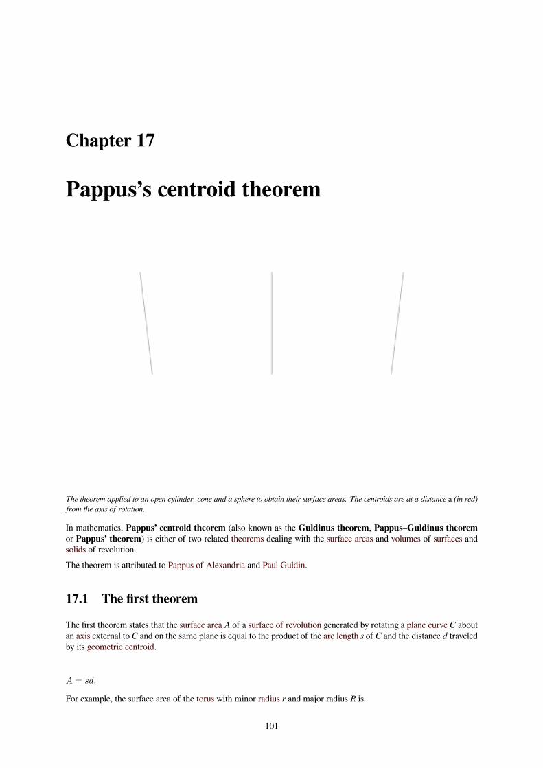
Chapter 17
Pappus’s centroid theorem
The theorem applied to an open cylinder, cone and a sphere to obtain their surface areas. The centroids are at a distance a (in red)from the axis of rotation.
In mathematics, Pappus’ centroid theorem (also known as the Guldinus theorem, Pappus–Guldinus theoremor Pappus’ theorem) is either of two related theorems dealing with the surface areas and volumes of surfaces andsolids of revolution.The theorem is attributed to Pappus of Alexandria and Paul Guldin.
17.1 The first theorem
The first theorem states that the surface area A of a surface of revolution generated by rotating a plane curve C aboutan axis external to C and on the same plane is equal to the product of the arc length s of C and the distance d traveledby its geometric centroid.
A = sd.
For example, the surface area of the torus with minor radius r and major radius R is
101
102 CHAPTER 17. PAPPUS’S CENTROID THEOREM
A = (2πr)(2πR) = 4π2Rr.
17.2 The second theorem
The second theorem states that the volume V of a solid of revolution generated by rotating a plane figure F about anexternal axis is equal to the product of the area A of F and the distance d traveled by its geometric centroid.
V = Ad.
For example, the volume of the torus with minor radius r and major radius R is
V = (πr2)(2πR) = 2π2Rr2.
17.3 Generalizations
The theorem can be generalized for arbitrary curves and shapes, under appropriate conditions.[1]
17.4 References[1] Goodman, A. W.; Goodman, G. “Generalizations of the Theorems of Pappus”. JSTOR. The American Mathematical
Monthly. Retrieved 2014-06-28.
17.5 External links• Weisstein, Eric W., “Pappus’s Centroid Theorem”, MathWorld.

Chapter 18
Rolle’s theorem
f’(c)=0
y = f(x)
a bc x
y
f(a)=f(b)
If a real-valued function ƒ is continuous on a closed interval [a, b], differentiable on the open interval (a, b), and ƒ(a) = ƒ(b), thenthere exists a c in the open interval (a, b) such that f'(c) = 0.
In calculus, Rolle’s theorem essentially states that any real-valued differentiable function that attains equal values attwo distinct points must have a stationary point somewhere between them—that is, a point where the first derivative(the slope of the tangent line to the graph of the function) is zero.
103

104 CHAPTER 18. ROLLE’S THEOREM
18.1 Standard version of the theorem
If a real-valued function f is continuous on a proper closed interval [a, b], differentiable on the open interval (a, b),and f(a) = f(b), then there exists at least one c in the open interval (a, b) such that
f ′(c) = 0
This version of Rolle’s theorem is used to prove the mean value theorem, of which Rolle’s theorem is indeed a specialcase. It is also the basis for the proof of Taylor’s theorem.
18.2 History
Indian mathematician Bhāskara II (1114–1185) is credited with knowledge of Rolle’s theorem.[1] The first knownformal proof was offered by Michel Rolle in 1691 and used the methods of differential calculus. The name “Rolle’stheorem” was first used by Moritz Wilhelm Drobisch of Germany in 1834 and by Giusto Bellavitis of Italy in 1846.[2]
18.3 Examples
18.3.1 First example
r
A semicircle of radius r.
For a radius r > 0, consider the functionf(x) =
√r2 − x2, x ∈ [−r, r].
Its graph is the upper semicircle centered at the origin. This function is continuous on the closed interval [−r,r] anddifferentiable in the open interval (−r,r), but not differentiable at the endpoints −r and r. Since f(−r) = f(r), Rolle’s

18.4. GENERALIZATION 105
theorem applies, and indeed, there is a point where the derivative of f is zero. Note that the theorem applies evenwhen the function cannot be differentiated at the endpoints because it only requires the function to be differentiablein the open interval.
18.3.2 Second example
1
2
3
4
−3 −2 −1 1 2 30
y = |x|
The graph of the absolute value function.
If differentiability fails at an interior point of the interval, the conclusion of Rolle’s theorem may not hold. Considerthe absolute value function
f(x) = |x|, x ∈ [−1, 1].
Then f(−1) = f(1), but there is no c between −1 and 1 for which the derivative is zero. This is because that function,although continuous, is not differentiable at x = 0. Note that the derivative of f changes its sign at x = 0, but withoutattaining the value 0. The theorem cannot be applied to this function, clearly, because it does not satisfy the con-dition that the function must be differentiable for every x in the open interval. However, when the differentiabilityrequirement is dropped from Rolle’s theorem, f will still have a critical number in the open interval (a,b), but it maynot yield a horizontal tangent (as in the case of the absolute value represented in the graph).
18.4 Generalization
The second example illustrates the following generalization of Rolle’s theorem:Consider a real-valued, continuous function f on a closed interval [a,b] with f(a) = f(b). If for every x in the openinterval (a,b) the right-hand limit
f ′(x+) := limh→0+
f(x+ h)− f(x)
h

106 CHAPTER 18. ROLLE’S THEOREM
and the left-hand limit
f ′(x−) := limh→0−
f(x+ h)− f(x)
h
exist in the extended real line [−∞,∞], then there is some number c in the open interval (a,b) such that one of thetwo limits
f ′(c+) and f ′(c−)
is ≥ 0 and the other one is ≤ 0 (in the extended real line). If the right- and left-hand limits agree for every x, thenthey agree in particular for c, hence the derivative of f exists at c and is equal to zero.
18.4.1 Remarks
1. If f is convex or concave, then the right- and left-hand derivatives exist at every inner point, hence the abovelimits exist and are real numbers.
2. This generalized version of the theorem is sufficient to prove convexity when the one-sided derivatives aremonotonically increasing:[3]
f ′(x−) ≤ f ′(x+) ≤ f ′(y−), x < y.
18.5 Proof of the generalized version
Since the proof for the standard version of Rolle’s theorem and the generalization are very similar, we prove thegeneralization.The idea of the proof is to argue that if f(a) = f(b), then f must attain either a maximum or a minimum somewherebetween a and b, say at c, and the function must change from increasing to decreasing (or the other way around) at c.In particular, if the derivative exists, it must be zero at c.By assumption, f is continuous on [a,b], and by the extreme value theorem attains both its maximum and its minimumin [a,b]. If these are both attained at the endpoints of [a,b], then f is constant on [a,b] and so the derivative of f iszero at every point in (a,b).Suppose then that the maximum is obtained at an interior point c of (a,b) (the argument for the minimum is verysimilar, just consider −f ). We shall examine the above right- and left-hand limits separately.For a real h such that c + h is in [a,b], the value f(c + h) is smaller or equal to f(c) because f attains its maximum atc. Therefore, for every h > 0,
f(c+ h)− f(c)
h≤ 0,
hence
f ′(c+) := limh→0+
f(c+ h)− f(c)
h≤ 0,
where the limit exists by assumption, it may be minus infinity.Similarly, for every h < 0, the inequality turns around because the denominator is now negative and we get
f(c+ h)− f(c)
h≥ 0,
18.6. GENERALIZATION TO HIGHER DERIVATIVES 107
hence
f ′(c−) := limh→0−
f(c+ h)− f(c)
h≥ 0,
where the limit might be plus infinity.Finally, when the above right- and left-hand limits agree (in particular when f is differentiable), then the derivativeof f at c must be zero.
18.6 Generalization to higher derivatives
We can also generalize Rolle’s theorem by requiring that f has more points with equal values and greater regularity.Specifically, suppose that
• the function f is n − 1 times continuously differentiable on the closed interval [a,b] and the nth derivative existson the open interval (a,b), and
• there are n intervals given by a1 < b1 ≤ a2 < b2 ≤ . . .≤ an < bn in [a,b] such that f(ak) = f(bk) for every kfrom 1 to n.
Then there is a number c in (a,b) such that the nth derivative of f at c is zero.The requirements concerning the nth derivative of f can be weakened as in the generalization above, giving thecorresponding (possibly weaker) assertions for the right- and left-hand limits defined above with f (n−1) in place of f.
18.6.1 Proof
The proof uses mathematical induction. For n = 1 is simply the standard version of Rolle’s theorem. As inductionhypothesis, assume the generalization is true for n − 1. We want to prove it for n > 1. By the standard version ofRolle’s theorem, for every integer k from 1 to n, there exists a ck in the open interval (ak,bk) such that f' (ck) = 0.Hence the first derivative satisfies the assumptions with the n − 1 closed intervals [c1,c2], . . ., [cn₋₁,cn]. By theinduction hypothesis, there is a c such that the (n − 1)st derivative of f' at c is zero.
18.7 Generalizations to other fields
Rolle’s theorem is a property of differentiable functions over the real numbers, which are an ordered field. As such,it does not generalize to other fields, but the following corollary does: if a real polynomial splits (has all its roots)over the real numbers, then its derivative does as well – one may call this property of a field Rolle’s property. Moregeneral fields do not always have a notion of differentiable function, but they do have a notion of polynomials, whichcan be symbolically differentiated. Similarly, more general fields may not have an order, but one has a notion of aroot of a polynomial lying in a field.Thus Rolle’s theorem shows that the real numbers have Rolle’s property, and any algebraically closed field such asthe complex numbers has Rolle’s property, but conversely the rational numbers do not – for example, x3 − x =x(x − 1)(x + 1) splits over the rationals, but its derivative 3x2 − 1 = 3(x − 1/
√3)(x + 1/
√3) does not. The
question of which fields satisfy Rolle’s property was raised in (Kaplansky 1972). For finite fields, the answer is thatonly F2 and F4 have Rolle’s property; this was first proven via technical means in (Craven & Csordas 1977), and asimple proof is given in (Ballantine & Roberts 2002).For a complex version, see Voorhoeve index.
18.8 See also• Mean value theorem

108 CHAPTER 18. ROLLE’S THEOREM
• Intermediate value theorem
• Linear interpolation
• Gauss-Lucas theorem
18.9 Notes[1] R.C. Gupta, Encyclopaedia of the History of Science, Technology, and Medicine in Non-Westen Cultures, p. 156.
[2] See Florian Cajori's A History of Mathematics, p. 224 .
[3] Artin, Emil (1964) [1931], The Gamma Function, trans. Michael Butler, Holt, Rinehart and Winston, pp. 3–4
18.10 References• Kaplansky, Irving (1972), Fields and Rings
• Craven, Thomas; Csordas, George (1977), “Multiplier sequences for fields”, Illinois J. Math. 21 (4): 801–817
• Ballantine, C.; Roberts, J. (January 2002), “A Simple Proof of Rolle’s Theorem for Finite Fields”, The Amer-ican Mathematical Monthly (Mathematical Association of America) 109 (1): 72–74, doi:10.2307/2695770,JSTOR 2695770
18.11 External links• Hazewinkel, Michiel, ed. (2001), “Rolle theorem”, Encyclopedia of Mathematics, Springer, ISBN 978-1-55608-010-4
• Rolle’s and Mean Value Theorems at cut-the-knot.

Chapter 19
Squeeze theorem
“Sandwich theorem” redirects here. For the result in measure theory, see Ham sandwich theorem.
In calculus, the squeeze theorem known also as the pinching theorem, the sandwich theorem, the sandwich ruleand sometimes the squeeze lemma is a theorem regarding the limit of a function.The squeeze theorem is used in calculus and mathematical analysis. It is typically used to confirm the limit of afunction via comparison with two other functions whose limits are known or easily computed. It was first usedgeometrically by the mathematicians Archimedes and Eudoxus in an effort to compute π, and was formulated inmodern terms by Gauss.In many languages (e.g. French, German and Italian), the squeeze theorem is also known as the two policemen (anda drunk) theorem, or some variation thereof. The story is that if two policemen are escorting a drunk prisonerbetween them, and both officers go to a cell, then (regardless of the path taken, and the fact that the prisoner may bewobbling about between the policemen) the prisoner must also end up in the cell.
19.1 Statement
The squeeze theorem is formally stated as follows.
Let I be an interval having the point a as a limit point. Let f, g, and h be functions defined on I,except possibly at a itself. Suppose that for every x in I not equal to a, we have:
g(x) ≤ f(x) ≤ h(x)
and also suppose that:
limx→a
g(x) = limx→a
h(x) = L.
Then limx→a f(x) = L.
• The functions g and h are said to be lower and upper bounds (respectively) of f.
• Here a is not required to lie in the interior of I. Indeed, if a is an endpoint of I, then the above limits are left-or right-hand limits.
• A similar statement holds for infinite intervals: for example, if I = (0, ∞), then the conclusion holds, taking thelimits as x →∞.
109

110 CHAPTER 19. SQUEEZE THEOREM
19.1.1 Proof
From the above hypotheses we have, taking the limit inferior and superior:
L = limx→a
g(x) ≤ lim infx→a
f(x) ≤ lim supx→a
f(x) ≤ limx→a
h(x) = L,
so all the inequalities are indeed equalities, and the thesis immediately follows.A direct proof, using the (ε, δ) definition of limit, would be to prove that for all real ε > 0 there exists a real δ > 0such that for all x with 0 < |x − a | < δ, we have −ε < f(x) − L < ε. Symbolically,
∀ε > 0 ∃ δ > 0 : ∀x (0 < |x− a| < δ ⇒ −ε < f(x)− L < ε).
As
limx→a
g(x) = L
means that
∀ε > 0 ∃ δ1 > 0 : ∀x (0 < |x− a| < δ1 ⇒ −ε < g(x)− L < ε). (1)
and
limx→a
h(x) = L
means that
∀ε > 0 ∃ δ2 > 0 : ∀x (0 < |x− a| < δ2 ⇒ −ε < h(x)− L < ε), (2)
then we have
g(x) ≤ f(x) ≤ h(x)
g(x)− L ≤ f(x)− L ≤ h(x)− L
We can choose δ := min δ1, δ2 . Then, if |x− a| < δ , combining (1) and (2), we have
−ε < g(x)− L ≤ f(x)− L ≤ h(x)− L < ε,
−ε < f(x)− L < ε
which completes the proof.
19.2 Examples
19.2.1 First example
The limit

19.2. EXAMPLES 111
x2 sin(1/ x) being squeezed in the limit as x goes to 0
limx→0
x2 sin( 1x )
cannot be determined through the limit law
limx→a
(f(x) · g(x)) = limx→a
f(x) · limx→a
g(x),
because
limx→0
sin( 1x )
does not exist.However, by the definition of the sine function,
−1 ≤ sin( 1x ) ≤ 1.
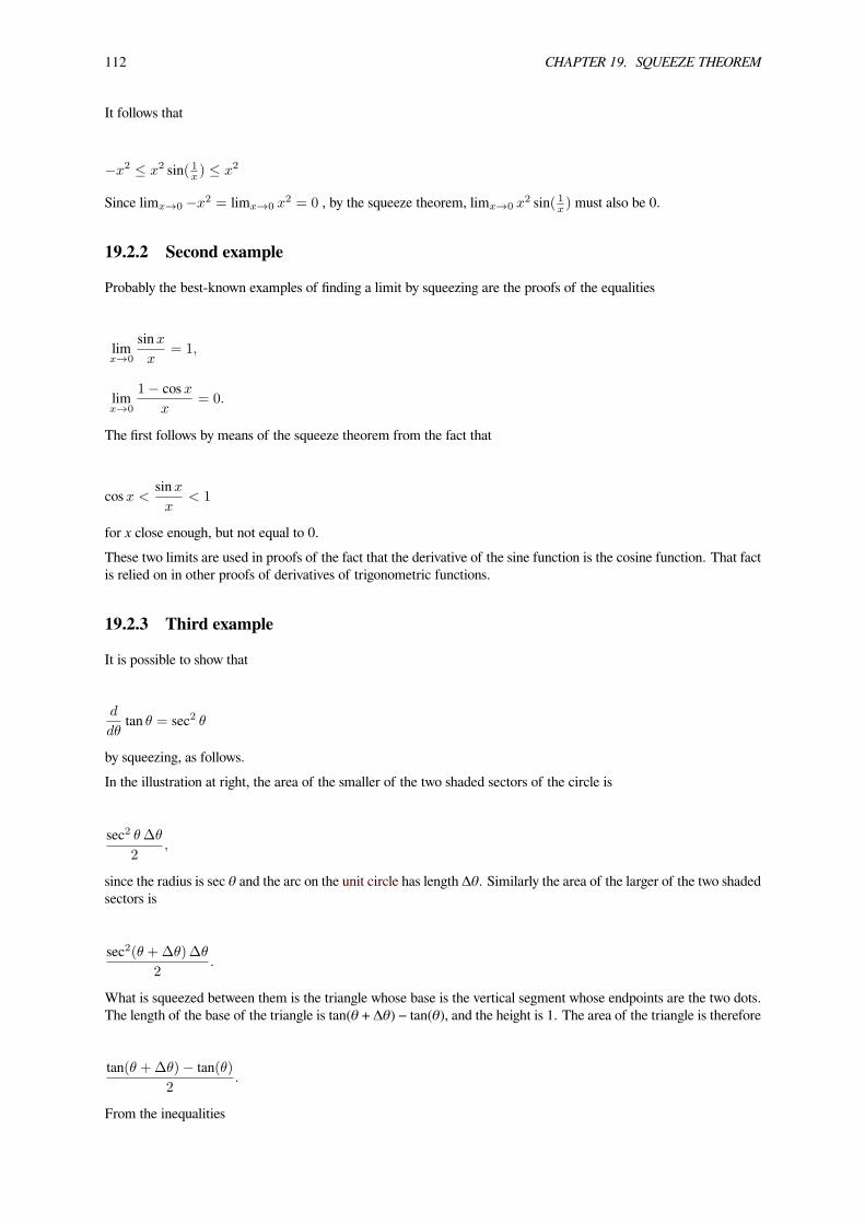
112 CHAPTER 19. SQUEEZE THEOREM
It follows that
−x2 ≤ x2 sin( 1x ) ≤ x2
Since limx→0 −x2 = limx→0 x2 = 0 , by the squeeze theorem, limx→0 x
2 sin( 1x ) must also be 0.
19.2.2 Second example
Probably the best-known examples of finding a limit by squeezing are the proofs of the equalities
limx→0
sinxx
= 1,
limx→0
1− cosxx
= 0.
The first follows by means of the squeeze theorem from the fact that
cosx < sinxx
< 1
for x close enough, but not equal to 0.These two limits are used in proofs of the fact that the derivative of the sine function is the cosine function. That factis relied on in other proofs of derivatives of trigonometric functions.
19.2.3 Third example
It is possible to show that
d
dθtan θ = sec2 θ
by squeezing, as follows.In the illustration at right, the area of the smaller of the two shaded sectors of the circle is
sec2 θ∆θ2
,
since the radius is sec θ and the arc on the unit circle has length Δθ. Similarly the area of the larger of the two shadedsectors is
sec2(θ +∆θ)∆θ
2.
What is squeezed between them is the triangle whose base is the vertical segment whose endpoints are the two dots.The length of the base of the triangle is tan(θ + Δθ) − tan(θ), and the height is 1. The area of the triangle is therefore
tan(θ +∆θ)− tan(θ)2
.
From the inequalities

19.2. EXAMPLES 113
1
tan θ (tan + Δθ )θsec θ
Δθ )+θ(sec
sec2 θ∆θ2
≤ tan(θ +∆θ)− tan(θ)2
≤ sec2(θ +∆θ)∆θ
2
we deduce that
sec2 θ ≤ tan(θ +∆θ)− tan(θ)∆θ
≤ sec2(θ +∆θ),
provided Δθ > 0, and the inequalities are reversed if Δθ < 0. Since the first and third expressions approach sec2θ asΔθ→ 0, and the middle expression approaches (d/dθ) tan θ, the desired result follows.
19.2.4 Fourth example
The squeeze theorem can still be used in multivariable calculus but the lower (and upper functions) must be below(and above) the target function not just along a path but around the entire neighborhood of the point of interest andit only works if the function really does have a limit there. It can, therefore, be used to prove that a function has alimit at a point, but it can never be used to prove that a function does not have a limit at a point.[1]
lim(x,y)→(0,0)
x2y
x2 + y2
114 CHAPTER 19. SQUEEZE THEOREM
cannot be found by taking any number of limits along paths that pass through the point, but since
0 ≤ x2
x2 + y2≤ 1
− |y| ≤ y ≤ |y|
− |y| ≤ x2y
x2 + y2≤ |y|
lim(x,y)→(0,0)
− |y| = 0
lim(x,y)→(0,0)
|y| = 0
0 ≤ lim(x,y)→(0,0)
x2y
x2 + y2≤ 0
therefore, by the squeeze theorem,
lim(x,y)→(0,0)
x2y
x2 + y2= 0
19.3 References• Weisstein, Eric W., “Squeezing Theorem”, MathWorld.
[1] Stewart, James (2008). “Chapter 15.2 Limits and Continuity”. Multivariable Calculus (6th ed.). pp. 909–910. ISBN0495011630.
19.4 External links• Squeeze Theorem by Bruce Atwood (Beloit College) after work by, Selwyn Hollis (Armstrong Atlantic StateUniversity), the Wolfram Demonstrations Project.
• Squeeze Theorem proof on Proofs.wiki.
Chapter 20
Stokes’ theorem
For the equation governing viscous drag in fluids, see Stokes’ law.
In vector calculus, and more generally differential geometry, Stokes’ theorem (also called the generalized Stokes’theorem) is a statement about the integration of differential forms onmanifolds, which both simplifies and generalizesseveral theorems from vector calculus. Stokes’ theorem says that the integral of a differential formω over the boundaryof some orientable manifold Ω is equal to the integral of its exterior derivative dω over the whole of Ω, i.e.,
∫∂Ω
ω =
∫Ω
dω.
This modern form of Stokes’ theorem is a vast generalization of a classical result. Lord Kelvin communicated it toGeorge Stokes in a letter dated July 2, 1850.[1][2][3] Stokes set the theorem as a question on the 1854 Smith’s Prizeexam, which led to the result bearing his name, even though it was actually first published by Hermann Hankel in1861.[3][4] This classical Kelvin–Stokes theorem relates the surface integral of the curl of a vector field F over a surfaceΣ in Euclidean three-space to the line integral of the vector field over its boundary ∂Σ:
∫∫Σ
∇× F · d =
∮∂Σ
F · dr.
This classical statement, along with the classical divergence theorem, fundamental theorem of calculus, and Green’stheorem are simply special cases of the general formulation stated above.
20.1 Introduction
The fundamental theorem of calculus states that the integral of a function f over the interval [a, b] can be calculatedby finding an antiderivative F of f :
∫ b
a
f(x) dx = F (b)− F (a).
Stokes’ theorem is a vast generalization of this theorem in the following sense.
• By the choice of F, dFdx = f(x) . In the parlance of differential forms, this is saying that f(x) dx is the exteriorderivative of the 0-form, i.e. function, F: in other words, that dF = f dx. The general Stokes theorem appliesto higher differential forms ω instead of just 0-forms such as F.
• A closed interval [a, b] is a simple example of a one-dimensional manifold with boundary. Its boundary is theset consisting of the two points a and b. Integrating f over the interval may be generalized to integrating formson a higher-dimensional manifold. Two technical conditions are needed: the manifold has to be orientable,and the form has to be compactly supported in order to give a well-defined integral.
115

116 CHAPTER 20. STOKES’ THEOREM
• The two points a and b form the boundary of the open interval. More generally, Stokes’ theorem appliesto oriented manifolds M with boundary. The boundary ∂M of M is itself a manifold and inherits a naturalorientation from that of the manifold. For example, the natural orientation of the interval gives an orientationof the two boundary points. Intuitively, a inherits the opposite orientation as b, as they are at opposite ends ofthe interval. So, “integrating” F over two boundary points a, b is taking the difference F(b) − F(a).
In even simpler terms, one can consider that points can be thought of as the boundaries of curves, that is as 0-dimensional boundaries of 1-dimensional manifolds. So, just as one can find the value of an integral (f dx = dF) overa 1-dimensional manifolds ([a, b]) by considering the anti-derivative (F) at the 0-dimensional boundaries ([a, b]), onecan generalize the fundamental theorem of calculus, with a few additional caveats, to deal with the value of integrals(dω) over n-dimensional manifolds (Ω) by considering the anti-derivative (ω) at the (n − 1)-dimensional boundaries(dΩ) of the manifold.So the fundamental theorem reads:
∫[a,b]
f(x) dx =
∫[a,b]
dF =
∫a−∪b+
F = F (b)− F (a).
20.2 General formulation
Let Ω be an oriented smooth manifold of dimension n and let α be an n-differential form that is compactly supportedon Ω. First, suppose that α is compactly supported in the domain of a single, oriented coordinate chart U, φ. Inthis case, we define the integral of α over Ω as
∫Ω
α =
∫ϕ(U)
(ϕ−1
)∗α,
i.e., via the pullback of α to Rn.More generally, the integral of α over Ω is defined as follows: Let ψi be a partition of unity associated with alocally finite cover Ui, φᵢ of (consistently oriented) coordinate charts, then define the integral
∫Ω
α ≡∑i
∫Ui
ψiα,
where each term in the sum is evaluated by pulling back to Rn as described above. This quantity is well-defined; thatis, it does not depend on the choice of the coordinate charts, nor the partition of unity.Stokes’ theorem reads: If ω is an (n − 1)-form with compact support on Ω and ∂Ω denotes the boundary of Ω withits induced orientation, then
∫Ω
dω =
∫∂Ω
ω
(=
∮∂Ω
ω
).
Here d is the exterior derivative, which is defined using the manifold structure only. On the r.h.s., a circle is sometimesused within the integral sign to stress the fact that the (n − 1)-manifold ∂Ω is closed.[5] The r.h.s. of the equation isoften used to formulate integral laws; the l.h.s. then leads to equivalent differential formulations (see below).The theorem is often used in situations where Ω is an embedded oriented submanifold of some bigger manifold onwhich the form ω is defined.A proof becomes particularly simple if the submanifold Ω is a so-called “normal manifold”, as in the figure on ther.h.s., which can be segmented into vertical stripes (e.g. parallel to the xn direction), such that after a partial integrationconcerning this variable, nontrivial contributions come only from the upper and lower boundary surfaces (colouredin yellow and red, respectively), where the complementary mutual orientations are visible through the arrows.

20.3. TOPOLOGICAL PRELIMINARIES; INTEGRATION OVER CHAINS 117
y
xa b
DC
C
C C
1
4
3
2
A “normal” integration manifold (here called D instead of Ω) for the special case n = 2
20.3 Topological preliminaries; integration over chains
Let M be a smooth manifold. A smooth singular k-simplex of M is a smooth map from the standard simplex in Rk
toM. The free abelian group, Sk, generated by singular k-simplices is said to consist of singular k-chains ofM. Thesegroups, together with the boundary map, ∂, define a chain complex. The corresponding homology (resp. cohomology)is called the smooth singular homology (resp. cohomology) of M.On the other hand, the differential forms, with exterior derivative, d, as the connecting map, form a cochain complex,which defines de Rham cohomology.Differential k-forms can be integrated over a k-simplex in a natural way, by pulling back toRk. Extending by linearityallows one to integrate over chains. This gives a linear map from the space of k-forms to the k-th group in the singularcochain, Sk*, the linear functionals on Sk. In other words, a k-form ω defines a functional
I(ω)(c) =
∮c
ω
on the k-chains. Stokes’ theorem says that this is a chain map from de Rham cohomology to singular cohomology; theexterior derivative, d, behaves like the dual of ∂ on forms. This gives a homomorphism from de Rham cohomologyto singular cohomology. On the level of forms, this means:

118 CHAPTER 20. STOKES’ THEOREM
1. closed forms, i.e., dω = 0, have zero integral over boundaries, i.e. over manifolds that can be written as∂∑
cMc , and
2. exact forms, i.e., ω = dσ, have zero integral over cycles, i.e. if the boundaries sum up to the empty set:∑c ∂Mc = ∅ .
De Rham’s theorem shows that this homomorphism is in fact an isomorphism. So the converse to 1 and 2 above holdtrue. In other words, if ci are cycles generating the k-th homology group, then for any corresponding real numbers,ai, there exist a closed form, ω, such that
∮ci
ω = ai,
and this form is unique up to exact forms.
20.4 Underlying principle
To simplify these topological arguments, it is worthwhile to examine the underlying principle by considering anexample for d = 2 dimensions. The essential idea can be understood by the diagram on the left, which shows that, inan oriented tiling of a manifold, the interior paths are traversed in opposite directions; their contributions to the pathintegral thus cancel each other pairwise. As a consequence, only the contribution from the boundary remains. It thussuffices to prove Stokes’ theorem for sufficiently fine tilings (or, equivalently, simplices), which usually is not difficult.
20.5 Special cases
The general form of the Stokes theorem using differential forms is more powerful and easier to use than the specialcases. The traditional versions can be formulated using Cartesian coordinates without the machinery of differentialgeometry, and thus are more accessible. Further, they are older and their names are more familiar as a result. Thetraditional forms are often considered more convenient by practicing scientists and engineers but the non-naturalnessof the traditional formulation becomes apparent when using other coordinate systems, even familiar ones like spher-ical or cylindrical coordinates. There is potential for confusion in the way names are applied, and the use of dualformulations.

20.5. SPECIAL CASES 119
20.5.1 Kelvin–Stokes theorem
z
x y
Σ
∂Σ
0
n
An illustration of the Kelvin–Stokes theorem, with surface Σ, its boundary ∂Σ and the “normal” vector n.
This is a (dualized) 1+1 dimensional case, for a 1-form (dualized because it is a statement about vector fields). Thisspecial case is often just referred to as the Stokes’ theorem in many introductory university vector calculus courses andas used in physics and engineering. It is also sometimes known as the curl theorem.The classical Kelvin–Stokes theorem:
∫Σ
∇× F · d =
∮∂Σ
F · dr,
which relates the surface integral of the curl of a vector field over a surface Σ in Euclidean three-space to the lineintegral of the vector field over its boundary, is a special case of the general Stokes theorem (with n = 2) once weidentify a vector field with a 1 form using the metric on Euclidean three-space. The curve of the line integral, ∂Σ,must have positive orientation, meaning that dr points counterclockwise when the surface normal, dΣ, points towardthe viewer, following the right-hand rule.One consequence of the Kelvin–Stokes theorem is that the field lines of a vector field with zero curl cannot be closedcontours. The formula can be rewritten as:

120 CHAPTER 20. STOKES’ THEOREM
∫∫Σ
(∂R
∂y− ∂Q
∂z
)dydz +
(∂P
∂z− ∂R
∂x
)dzdx+
(∂Q
∂x− ∂P
∂y
)dxdy
=
∮∂Σ
Pdx+Qdy +Rdz ,
where P, Q and R are the components of F.These variants are rarely used:
∫Σ
[g (∇× F) + (∇g)× F] · d =
∮∂Σ
gF · dr,
∫Σ
[F (∇ ·G)−G (∇ · F) + (G · ∇)F− (F · ∇)G] · d =
∮∂Σ
(F×G) · dr.∫Σ
∇(F · d )− (∇ · F)d =
∮∂Σ
dr× F.
20.5.2 Green’s theorem
Green’s theorem is immediately recognizable as the third integrand of both sides in the integral in terms of P, Q, andR cited above.
In electromagnetism
Two of the four Maxwell equations involve curls of 3-D vector fields and their differential and integral forms arerelated by the Kelvin–Stokes theorem. Caution must be taken to avoid cases with moving boundaries: the partialtime derivatives are intended to exclude such cases. If moving boundaries are included, interchange of integrationand differentiation introduces terms related to boundary motion not included in the results below (see Differentiationunder the integral sign):The above listed subset of Maxwell’s equations are valid for electromagnetic fields expressed in SI units. In othersystems of units, such as CGS or Gaussian units, the scaling factors for the terms differ. For example, in Gaussianunits, Faraday’s law of induction and Ampère’s law take the forms[6][7]
∇× E = −1
c
∂B∂t,
∇×H =1
c
∂D∂t
+4π
cJ,
respectively, where c is the speed of light in vacuum.
20.5.3 Divergence theorem
Likewise, the Ostrogradsky–Gauss theorem (also known as the divergence theorem or Gauss’s theorem)
∫Vol
∇ · F dVol =∮∂Vol
F · d
is a special case if we identify a vector field with the n−1 form obtained by contracting the vector field with theEuclidean volume form. An application of this is the case F = fc where c is an arbitrary constant vector. Workingout the divergence of the product gives

20.6. NOTES 121
c ·∫Vol
∇f dVol = c ·∮∂Vol
fd
Since this holds for all c, we find
∫Vol
∇f dVol =∮∂Vol
fd
20.6 Notes[1] See:
• Victor J. Katz (May 1979) “The history of Stokes’ theorem,” Mathematics Magazine, 52 (3): 146–156.• The letter from Thomson to Stokes appears in: William Thomson and George Gabriel Stokes with David B. Wilson,ed., The Correspondence between Sir George Gabriel Stokes and Sir William Thomson, Baron Kelvin of Largs, Volume1: 1846–1869 (Cambridge, England: Cambridge University Press, 1990), pages 96–97.
• Neither Thomson nor Stokes published a proof of the theorem. The first published proof appeared in 1861 in:Hermann Hankel, Zur allgemeinen Theorie der Bewegung der Flüssigkeiten [On the general theory of the movementof fluids] (Göttingen, (Germany): Dieterische University Buchdruckerei, 1861); see pages 34–37. Hankel doesn'tmention the author of the theorem.
• In a footnote, Larmor mentions earlier researchers who had integrated, over a surface, the curl of a vector field. See:George G. Stokes with Sir Joseph Larmor and John Wm. Strutt (Baron Rayleigh), ed.s, Mathematical and PhysicalPapers by the late Sir George Gabriel Stokes, ... (Cambridge, England: University of Cambridge Press, 1905), vol. 5,pages 320–321.
[2] Olivier Darrigol,Electrodynamics from Ampere to Einstein, p. 146,ISBN 0198505930 Oxford (2000)
[3] Spivak (1965), p. vii, Preface.
[4] See:
• The 1854 Smith’s Prize Examination is available on-line at: Clerk Maxwell Foundation. Maxwell took this exami-nation and tied for first place with Edward John Routh in the Smith’s Prize examination of 1854. See footnote 2 onpage 237 of: James ClerkMaxwell with P. M. Harman, ed., The Scientific Letters and Papers of James Clerk Maxwell,Volume I: 1846–1862 (Cambridge, England: Cambridge University Press, 1990), page 237; see also Wikipedia’sarticle "Smith’s prize" or the Clerk Maxwell Foundation.
• James Clerk Maxwell, A Treatise on Electricity and Magnetism (Oxford, England: Clarendon Press,1873), volume 1,pages 25–27. In a footnote on page 27, Maxwell mentions that Stokes used the theorem as question 8 in the Smith’sPrize Examination of 1854. This footnote appears to have been the cause of the theorem’s being known as “Stokes’theorem”.
[5] For mathematicians this fact is known, therefore the circle is redundant and often omitted. However, one should keep inmind here that in thermodynamics, where frequently expressions as
∮W
d totalU appear (wherein the total derivative,see below, should not be confused with the exterior one), the integration pathW is a one-dimensional closed line on a muchhigher-dimensional manifold. That is, in a thermodynamic application, whereU is a function of the temperature α1 := T ,the volumeα2 := V, and the electrical polarizationα3 := P of the sample, one has d totalU =
∑3i=1
∂U∂αi
dαi, and thecircle is really necessary, e.g. if one considers the differential consequences of the integral postulate
∮W
d totalU !=0.
[6] J.D. Jackson, Classical Electrodynamics, 2nd Ed (Wiley, New York, 1975).
[7] M. Born and E. Wolf, Principles of Optics, 6th Ed. (Cambridge University Press, Cambridge, 1980).
20.7 Further reading
• Joos, Georg. Theoretische Physik. 13th ed. Akademische Verlagsgesellschaft Wiesbaden 1980. ISBN 3-400-00013-2

122 CHAPTER 20. STOKES’ THEOREM
• Katz, Victor J. (May 1979), “The History of Stokes’ Theorem”, Mathematics Magazine 52 (3): 146–156,doi:10.2307/2690275
• Marsden, Jerrold E., Anthony Tromba. Vector Calculus. 5th edition W. H. Freeman: 2003.
• Lee, John. Introduction to Smooth Manifolds. Springer-Verlag 2003. ISBN 978-0-387-95448-6
• Rudin, Walter (1976), Principles of Mathematical Analysis, New York: McGraw–Hill, ISBN 0-07-054235-X
• Spivak, Michael (1965), Calculus on Manifolds: A Modern Approach to Classical Theorems of Advanced Cal-culus, HarperCollins, ISBN 978-0-8053-9021-6
• Stewart, James. Calculus: Concepts and Contexts. 2nd ed. Pacific Grove, CA: Brooks/Cole, 2001.
• Stewart, James. Calculus: Early Transcendental Functions. 5th ed. Brooks/Cole, 2003.
20.8 External links• Hazewinkel, Michiel, ed. (2001), “Stokes formula”, Encyclopedia of Mathematics, Springer, ISBN 978-1-55608-010-4
• Proof of the Divergence Theorem and Stokes’ Theorem
• Calculus 3 – Stokes Theorem from lamar.edu – an expository explanation
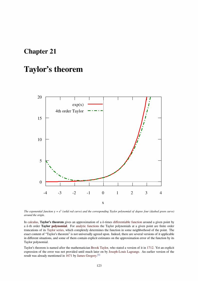
Chapter 21
Taylor’s theorem
0
5
10
15
20
-4 -3 -2 -1 0 1 2 3 4
x
exp(x) 4th order Taylor
The exponential function y = ex (solid red curve) and the corresponding Taylor polynomial of degree four (dashed green curve)around the origin.
In calculus, Taylor’s theorem gives an approximation of a k-times differentiable function around a given point bya k-th order Taylor polynomial. For analytic functions the Taylor polynomials at a given point are finite ordertruncations of its Taylor series, which completely determines the function in some neighborhood of the point. Theexact content of “Taylor’s theorem” is not universally agreed upon. Indeed, there are several versions of it applicablein different situations, and some of them contain explicit estimates on the approximation error of the function by itsTaylor polynomial.Taylor’s theorem is named after the mathematician Brook Taylor, who stated a version of it in 1712. Yet an explicitexpression of the error was not provided until much later on by Joseph-Louis Lagrange. An earlier version of theresult was already mentioned in 1671 by James Gregory.[1]
123

124 CHAPTER 21. TAYLOR’S THEOREM
Taylor’s theorem is taught in introductory level calculus courses and it is one of the central elementary tools inmathematical analysis. Within pure mathematics it is the starting point of more advanced asymptotic analysis, andit is commonly used in more applied fields of numerics as well as in mathematical physics. Taylor’s theorem alsogeneralizes to multivariate and vector valued functions f : Rn → Rm on any dimensions n and m. This generalizationof Taylor’s theorem is the basis for the definition of so-called jets which appear in differential geometry and partialdifferential equations.
21.1 Motivation
Graph of f(x) = ex (blue) with its linear approximation P1(x) = 1 + x (red) at a = 0.
If a real-valued function f is differentiable at the point a then it has a linear approximation at the point a. This meansthat there exists a function h1 such that
f(x) = f(a) + f ′(a)(x− a) + h1(x)(x− a), limx→a
h1(x) = 0.
Here
P1(x) = f(a) + f ′(a)(x− a)
is the linear approximation of f at the point a. The graph of y = P1(x) is the tangent line to the graph of f at x = a.The error in the approximation is
R1(x) = f(x)− P1(x) = h1(x)(x− a).
Note that this goes to zero a little bit faster than x − a as x tends to a, given the limiting behavior of h1.If we wanted a better approximation to f, we might instead try a quadratic polynomial instead of a linear function.Instead of just matching one derivative of f at a, we can match two derivatives, thus producing a polynomial that hasthe same slope and concavity as f at a. The quadratic polynomial in question is

21.1. MOTIVATION 125
Graph of f(x)=ex (blue) with its quadratic approximation P2(x) = 1 + x + x2/2 (red) at a = 0. Note the improvement in theapproximation.
P2(x) = f(a) + f ′(a)(x− a) +f ′′(a)
2(x− a)2.
Taylor’s theorem ensures that the quadratic approximation is, in a sufficiently small neighborhood of the point a, abetter approximation than the linear approximation. Specifically,
f(x) = P2(x) + h2(x)(x− a)2, limx→a
h2(x) = 0.
Here the error in the approximation is
R2(x) = f(x)− P2(x) = h2(x)(x− a)2
which, given the limiting behavior of h2, goes to zero faster than (x − a)2 as x tends to a.Similarly, we get still better approximations to f if we use polynomials of higher degree, since then we can match evenmore derivatives with f at the selected base point. In general, the error in approximating a function by a polynomialof degree k will go to zero a little bit faster than (x − a)k as x tends to a.This result is of asymptotic nature: it only tells us that the error Rk in an approximation by a k-th order Taylorpolynomial Pk tends to zero faster than any nonzero k-th degree polynomial as x→ a. It does not tell us how large theerror is in any concrete neighborhood of the center of expansion, but for this purpose there are explicit formulae forthe remainder term (given below) which are valid under some additional regularity assumptions on f. These enhancedversions of Taylor’s theorem typically lead to uniform estimates for the approximation error in a small neighborhoodof the center of expansion, but the estimates do not necessarily hold for neighborhoods which are too large, even ifthe function f is analytic. In that situation one may have to select several Taylor polynomials with different centersof expansion to have reliable Taylor-approximations of the original function (see animation on the right.)There are several things we might do with the remainder term:
1. Estimate the error in using a polynomial P (x) of degree k to estimate f(x) on a given interval (a - r, a + r).(The interval and the degree k are fixed; we want to find the error.)

126 CHAPTER 21. TAYLOR’S THEOREM
Approximation of f(x) = 1/(1 + x2) by its Taylor polynomials P of order k = 1, ..., 16 centered at x = 0 (red) and x = 1 (green).The approximations do not improve at all outside (−1,1) and (1-√2,1+√2), respectively.
2. Find the smallest degree k for which the polynomial P (x) approximates f(x) to within a given error (or toler-ance) on a given interval (a - r, a + r) . (The interval and the error are fixed; we want to find the degree.)
3. Find the largest interval (a - r, a + r) on which P (x) approximates f(x) to within a given error (“tolerance”).(The degree and the error are fixed; we want to find the interval.)
It is also possible that increasing the degree of the approximating polynomial does not increase the quality of ap-proximation at all even if the function f to be approximated is infinitely many times differentiable. An example ofthis behavior is given below, and it is related to the fact that unlike analytic functions, more general functions are not(locally) determined by the values of their derivatives at a single point.
21.2 Taylor’s theorem in one real variable
21.2.1 Statement of the theorem
The precise statement of the most basic version of Taylor’s theorem is as follows:
Taylor’s theorem.[2][3][4] Let k ≥ 1 be an integer and let the function f : R → R be k timesdifferentiable at the point a ∈ R. Then there exists a function hk : R→ R such that
f(x) = f(a) + f ′(a)(x− a) +f ′′(a)
2!(x− a)2 + · · ·+ f (k)(a)
k!(x− a)k + hk(x)(x− a)k,
and limx→a hk(x) = 0. This is called the Peano form of the remainder.
The polynomial appearing in Taylor’s theorem is the k-th order Taylor polynomial
Pk(x) = f(a) + f ′(a)(x− a) +f ′′(a)
2!(x− a)2 + · · ·+ f (k)(a)
k!(x− a)k
of the function f at the point a. The Taylor polynomial is the unique “asymptotic best fit” polynomial in the sensethat if there exists a function hk : R→ R and a k-th order polynomial p such that
f(x) = p(x) + hk(x)(x− a)k, limx→a
hk(x) = 0,

21.2. TAYLOR’S THEOREM IN ONE REAL VARIABLE 127
then p = Pk. Taylor’s theorem describes the asymptotic behavior of the remainder term
Rk(x) = f(x)− Pk(x),
which is the approximation error when approximating f with its Taylor polynomial. Using the little-o notation thestatement in Taylor’s theorem reads as
Rk(x) = o(|x− a|k), x→ a.
21.2.2 Explicit formulae for the remainder
Under stronger regularity assumptions on f there are several precise formulae for the remainder term Rk of the Taylorpolynomial, the most common ones being the following.
Mean-value forms of the remainder. Let f : R → R be k+1 times differentiable on the openinterval with f(k) continuous on the closed interval between a and x. Then
Rk(x) =f (k+1)(ξL)
(k + 1)!(x− a)k+1
for some real number ξL between a and x. This is the Lagrange form[5] of the remainder. Similarly,
Rk(x) =f (k+1)(ξC)
k!(x− ξC)
k(x− a)
for some real number ξC between a and x. This is the Cauchy form[6] of the remainder.
These refinements of Taylor’s theorem are usually proved using the mean value theorem, whence the name. Alsoother similar expressions can be found. For example, if G(t) is continuous on the closed interval and differentiablewith a non-vanishing derivative on the open interval between a and x, then
Rk(x) =f (k+1)(ξ)
k!(x− ξ)k
G(x)−G(a)
G′(ξ)
for some number ξ between a and x. This version covers the Lagrange and Cauchy forms of the remainder as specialcases, and is proved below using Cauchy’s mean value theorem.The statement for the integral form of the remainder is more advanced than the previous ones, and requires under-standing of Lebesgue integration theory for the full generality. However, it holds also in the sense of Riemann integralprovided the (k+1)-st derivative of f is continuous on the closed interval [a,x].
Integral form of the remainder.[7] Let f(k) be absolutely continuous on the closed interval betweena and x. Then
Rk(x) =
∫ x
a
f (k+1)(t)
k!(x− t)k dt.
Due to absolute continuity of f(k) on the closed interval between a and x its derivative f(k+1) exists as an L1-function,and the result can be proven by a formal calculation using fundamental theorem of calculus and integration by parts.
21.2.3 Estimates for the remainder
It is often useful in practice to be able to estimate the remainder term appearing in the Taylor approximation, ratherthan having an exact formula for it. Suppose that f is (k+1)-times continuously differentiable in an interval I containinga. Suppose that there are real constants q and Q such that
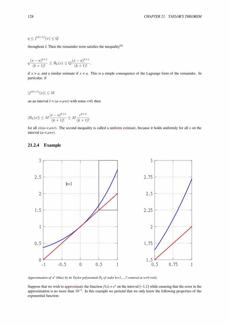
128 CHAPTER 21. TAYLOR’S THEOREM
q ≤ f (k+1)(x) ≤ Q
throughout I. Then the remainder term satisfies the inequality[8]
q(x− a)k+1
(k + 1)!≤ Rk(x) ≤ Q
(x− a)k+1
(k + 1)!,
if x > a, and a similar estimate if x < a. This is a simple consequence of the Lagrange form of the remainder. Inparticular, if
|f (k+1)(x)| ≤M
on an interval I = (a−r,a+r) with some r>0, then
|Rk(x)| ≤M|x− a|k+1
(k + 1)!≤M
rk+1
(k + 1)!
for all x∈(a−r,a+r). The second inequality is called a uniform estimate, because it holds uniformly for all x on theinterval (a−r,a+r).
21.2.4 Example
Approximation of ex (blue) by its Taylor polynomials P of order k=1,...,7 centered at x=0 (red).
Suppose that we wish to approximate the function f(x) = ex on the interval [−1,1] while ensuring that the error in theapproximation is no more than 10−5. In this example we pretend that we only know the following properties of theexponential function:
21.3. RELATIONSHIP TO ANALYTICITY 129
(∗) e0 = 1,d
dxex = ex, ex > 0, x ∈ R.
From these properties it follows that f(k)(x) = ex for all k, and in particular, f(k)(0) = 1. Hence the k-th order Taylorpolynomial of f at 0 and its remainder term in the Lagrange form are given by
Pk(x) = 1 + x+x2
2!+ · · ·+ xk
k!, Rk(x) =
eξ
(k + 1)!xk+1,
where ξ is some number between 0 and x. Since ex is increasing by (*), we can simply use ex ≤ 1 for x ∈ [−1, 0] toestimate the remainder on the subinterval [−1, 0]. To obtain an upper bound for the remainder on [0,1], we use theproperty eξ<ex for 0<ξ<x to estimate
ex = 1 + x+eξ
2x2 < 1 + x+
ex
2x2, 0 < x ≤ 1
using the second order Taylor expansion. Then we solve for ex to deduce that
ex ≤ 1 + x
1− x2
2
= 21 + x
2− x2≤ 4, 0 ≤ x ≤ 1
simply by maximizing the numerator and minimizing the denominator. Combining these estimates for ex we see that
|Rk(x)| ≤4|x|k+1
(k + 1)!≤ 4
(k + 1)!, −1 ≤ x ≤ 1,
so the required precision is certainly reached, when
4
(k + 1)!< 10−5 ⇔ 4 · 105 < (k + 1)! ⇔ k ≥ 9.
(See factorial or compute by hand the values 9!=362 880 and 10!=3 628 800.) As a conclusion, Taylor’s theoremleads to the approximation
ex = 1 + x+x2
2!+ . . .+
x9
9!+R9(x), |R9(x)| < 10−5, −1 ≤ x ≤ 1.
For instance, this approximation provides a decimal expression e≈2.71828, correct up to five decimal places.
21.3 Relationship to analyticity
21.3.1 Taylor expansions of real analytic functions
Let I⊂R be an open interval. By definition, a function f:I→R is real analytic if it is locally defined by a convergentpower series. This means that for every a ∈ I there exists some r > 0 and a sequence of coefficients ck ∈ R such that(a − r, a + r) ⊂ I and
f(x) =
∞∑k=0
ck(x− a)k = c0 + c1(x− a) + c2(x− a)2 + · · · , |x− a| < r.
In general, the radius of convergence of a power series can be computed from the Cauchy–Hadamard formula

130 CHAPTER 21. TAYLOR’S THEOREM
1
R= lim sup
k→∞|ck|
1k .
This result is based on comparison with a geometric series, and the same method shows that if the power series basedon a converges for some b∈R, it must converge uniformly on the closed interval [a − rb, a + rb], where rb = |b − a|.Here only the convergence of the power series is considered, and it might well be that (a − R,a + R) extends beyondthe domain I of f.The Taylor polynomials of the real analytic function f at a are simply the finite truncations
Pk(x) =k∑
j=0
cj(x− a)j , cj =f (j)(a)
j!
of its locally defining power series, and the corresponding remainder terms are locally given by the analytic functions
Rk(x) =∞∑
j=k+1
cj(x− a)j = (x− a)khk(x), |x− a| < r.
Here the functions
hk : (a− r, a+ r) → R; hk(x) = (x− a)
∞∑j=0
ck+1+j(x− a)j
are also analytic, since their defining power series have the same radius of convergence as the original series. Assumingthat [a − r, a + r] ⊂ I and r < R, all these series converge uniformly on (a − r, a + r). Naturally, in the case of analyticfunctions one can estimate the remainder term Rk(x) by the tail of the sequence of the derivatives f′ (a) at the centerof the expansion, but using complex analysis also another possibility arises, which is described below.
21.3.2 Taylor’s theorem and convergence of Taylor series
There is a source of confusion on the relationship between Taylor polynomials of smooth functions and the Taylorseries of analytic functions. One can (rightfully) see the Taylor series
f(x) ≈∞∑k=0
ck(x− a)k = c0 + c1(x− a) + c2(x− a)2 + . . .
of an infinitely many times differentiable function f:R→R as its “infinite order Taylor polynomial” at a. Now theestimates for the remainder of a Taylor polynomial implies that for any order k and for any r>0 there exists a constantMk,r>0 such that
(∗) |Rk(x)| ≤Mk,r|x− a|k+1
(k + 1)!
for every x∈(a-r,a+r). Sometimes these constants can be chosen in such way thatMk,r → 0 when k→∞ and r staysfixed. Then the Taylor series of f converges uniformly to some analytic function
Tf : (a− r, a+ r) → R; Tf (x) =∞∑k=0
f (k)(a)
k!(x− a)k.
Here comes the subtle point. It may well be that an infinitely many times differentiable function f has a Taylor seriesat a which converges on some open neighborhood of a, but the limit function Tf is different from f. An importantexample of this phenomenon is provided by
21.3. RELATIONSHIP TO ANALYTICITY 131
f : R → R; f(x) =
e−
1x2 x > 0,
0 x ≤ 0.
Using the chain rule one can show inductively that for any order k,
f (k)(x) =
pk(x)x3k e−
1x2 x > 0
0 x ≤ 0
for some polynomial pk of degree 2(k-1). The function e− 1x2 tends to zero faster than any polynomial as x→ 0, so f
is infinitely many times differentiable and f (k)(0) = 0 for every positive integer k. Now the estimates for the remainderfor the Taylor polynomials show that the Taylor series of f converges uniformly to the zero function on the whole realaxis. Nothing is wrong in here:
• The Taylor series of f converges uniformly to the zero function Tf(x)=0.
• The zero function is analytic and every coefficient in its Taylor series is zero.
• The function f is infinitely many times differentiable, but not analytic.
• For any k∈N and r>0 there exists Mk,r>0 such that the remainder term for the k-th order Taylor polynomialof f satisfies (*).
21.3.3 Taylor’s theorem in complex analysis
Taylor’s theorem generalizes to functions f : C → C which are complex differentiable in an open subset U ⊂ Cof the complex plane. However, its usefulness is dwarfed by other general theorems in complex analysis. Namely,stronger versions of related results can be deduced for complex differentiable functions f : U → C using Cauchy’sintegral formula as follows.Let r > 0 such that the closed disk B(z, r) ∪ S(z, r) is contained in U. Then Cauchy’s integral formula with a positiveparametrization γ(t)=z + reit of the circle S(z,r) with t ∈ [0,2π] gives
f(z) =1
2πi
∫γ
f(w)
w − zdw, f ′(z) =
1
2πi
∫γ
f(w)
(w − z)2dw,
. . . , f (k)(z) =k!
2πi
∫γ
f(w)
(w − z)k+1dw.
Here all the integrands are continuous on the circle S(z, r), which justifies differentiation under the integral sign. Inparticular, if f is once complex differentiable on the open set U, then it is actually infinitely many times complexdifferentiable on U. One also obtains the Cauchy’s estimates[9]
|f (k)(z)| ≤ k!
2π
∫γ
Mr
|w − z|k+1dw =
k!Mr
rk, Mr = max
|w−c|=r|f(w)|
for any z ∈ U and r > 0 such that B(z, r) ∪ S(c, r) ⊂ U. These estimates imply that the complex Taylor series
Tf (z) =∞∑k=0
f (k)(c)
k!(z − c)k
of f converges uniformly on any open disk B(c, r) ⊂ U with S(c, r) ⊂ U into some function Tf. Furthermore, usingthe contour integral formulae for the derivatives f(k)(c),
132 CHAPTER 21. TAYLOR’S THEOREM
Tf (z) =
∞∑k=0
(z − c)k
2πi
∫γ
f(w)
(w − c)k+1dw =
1
2πi
∫γ
f(w)
w − c
∞∑k=0
(z − c
w − c
)k
dw
=1
2πi
∫γ
f(w)
w − c
(1
1− z−cw−c
)dw =
1
2πi
∫γ
f(w)
w − zdw = f(z),
so any complex differentiable function f in an open set U ⊂ C is in fact complex analytic. All that is said for realanalytic functions here holds also for complex analytic functions with the open interval I replaced by an open subsetU ∈ C and a-centered intervals (a − r, a + r) replaced by c-centered disks B(c, r). In particular, the Taylor expansionholds in the form
f(z) = Pk(z) +Rk(z), Pk(z) =
k∑j=0
f (j)(c)
j!(z − c)j ,
where the remainder term Rk is complex analytic. Methods of complex analysis provide some powerful resultsregarding Taylor expansions. For example, using Cauchy’s integral formula for any positively oriented Jordan curveγ which parametrizes the boundary ∂W ⊂ U of a regionW ⊂ U, one obtains expressions for the derivatives f(j)(c) asabove, and modifying slightly the computation for Tf(z) = f(z), one arrives at the exact formula
Rk(z) =
∞∑j=k+1
(z − c)j
2πi
∫γ
f(w)
(w − c)j+1dw =
(z − c)k+1
2πi
∫γ
f(w)dw
(w − c)k+1(w − z), z ∈W.
The important feature here is that the quality of the approximation by a Taylor polynomial on the region W ⊂ U isdominated by the values of the function f itself on the boundary ∂W ⊂ U. Similarly, applying Cauchy’s estimates tothe series expression for the remainder, one obtains the uniform estimates
|Rk(z)| ≤∞∑
j=k+1
Mr|z − c|j
rj=
Mr
rk+1
|z − c|k+1
1− |z−c|r
≤ Mrβk+1
1− β,
|z − c|r
≤ β < 1.
21.3.4 Example
The function f:R→R defined by
f(x) =1
1 + x2
is real analytic, that is, locally determined by its Taylor series. This function was plotted above to illustrate the factthat some elementary functions cannot be approximated by Taylor polynomials in neighborhoods of the center ofexpansion which are too large. This kind of behavior is easily understood in the framework of complex analysis.Namely, the function f extends into a meromorphic function
f : C ∪ ∞ → C ∪ ∞; f(z) =1
1 + z2
on the compactified complex plane. It has simple poles at z=i and z=−i, and it is analytic elsewhere. Now its Taylorseries centered at z0 converges on any disc B(z0,r) with r<|z-z0|, where the same Taylor series converges at z∈C.Therefore Taylor series of f centered at 0 converges on B(0,1) and it does not converge for any z∈C with |z|>1 dueto the poles at i and −i. For the same reason the Taylor series of f centered at 1 converges on B(1,√2) and does notconverge for any z∈C with |z−1|>√2.

21.4. GENERALIZATIONS OF TAYLOR’S THEOREM 133
Complex plot of f(z) = 1/(1 + z2). Modulus is shown by elevation and argument by coloring: cyan=0, blue=π/3, violet=2π/3,red=π, yellow=4π/3, green=5π/3.
21.4 Generalizations of Taylor’s theorem
21.4.1 Higher-order differentiability
A function f: Rn → R is differentiable at a ∈ Rn if and only if there exists a linear functional L : Rn → R and afunction h : Rn → R such that
f(x) = f(a) + L(x− a) + h(x)|x− a|, limx→a
h(x) = 0.
If this is the case, then L = df(a) is the (uniquely defined) differential of f at the point a. Furthermore, then the partialderivatives of f exist at a and the differential of f at a is given by
df(a)(v) =∂f
∂x1(a)v1 + · · ·+ ∂f
∂xn(a)vn.
Introduce the multi-index notation
|α| = α1 + · · ·+ αn, α! = α1! · · ·αn!, xα = xα11 · · ·xαn
n
for α ∈ Nn and x ∈ Rn. If all the k-th order partial derivatives of f : Rn → R are continuous at a ∈ Rn, then byClairaut’s theorem, one can change the order of mixed derivatives at a, so the notation
134 CHAPTER 21. TAYLOR’S THEOREM
Dαf =∂|α|f
∂xα11 · · · ∂xαn
n, |α| ≤ k
for the higher order partial derivatives is justified in this situation. The same is true if all the (k − 1)-th order par-tial derivatives of f exist in some neighborhood of a and are differentiable at a.[10] Then we say that f is k timesdifferentiable at the point a .
21.4.2 Taylor’s theorem for multivariate functionsMultivariate version of Taylor’s theorem.[11] Let f : Rn → R be a k times differentiable function
at the point a∈Rn. Then there exists hα : Rn→R such that
f(x) =∑|α|≤k
Dαf(a)
α!(x− a)α +
∑|α|=k
hα(x)(x− a)α,
and limx→a
hα(x) = 0.
If the function f : Rn → R is k+1 times continuously differentiable in the closed ball B, then one can derive an exactformula for the remainder in terms of (k+1)-th order partial derivatives of f in this neighborhood. Namely,
f(x) =∑|α|≤k
Dαf(a)
α!(x− a)α +
∑|β|=k+1
Rβ(x)(x− a)β ,
Rβ(x) =|β|β!
∫ 1
0
(1− t)|β|−1Dβf(a+ t(x− a)
)dt.
In this case, due to the continuity of (k+1)-th order partial derivatives in the compact set B, one immediately obtainsthe uniform estimates
|Rβ(x)| ≤1
β!max
|α|=|β|maxy∈B
|Dαf(y)|, x ∈ B.
21.4.3 Example in two dimensions
For example, the third order Taylor polynomial of a function f: R2 → R is, denoting x − a = v,
P3(x) = f(a)+∂f
∂x1(a)v1 +
∂f
∂x2(a)v2 +
∂2f
∂2x1(a)
v212!
+∂2f
∂x1∂x2(a)v1v2 +
∂2f
∂2x2(a)
v222!
+∂3f
∂x31(a)
v313!
+∂3f
∂2x1∂x2(a)
v21v22!
+∂3f
∂x1∂2x2(a)
v1v22
2!+
∂3f
∂3x2(a)
v323!
21.5 Proofs
21.5.1 Proof for Taylor’s theorem in one real variable
Let[12]
hk(x) =
f(x)−P (x)(x−a)k
x = a
0 x = a
where, as in the statement of Taylor’s theorem,

21.5. PROOFS 135
P (x) = f(a) + f ′(a)(x− a) +f ′′(a)
2!(x− a)2 + · · ·+ f (k)(a)
k!(x− a)k.
It is sufficient to show that
limx→a
hk(x) = 0.
The proof here is based on repeated application of L'Hôpital’s rule. Note that, for each j = 0,1,...,k−1, f (j)(a) =P (j)(a) . Hence each of the first k−1 derivatives of the numerator in hk(x) vanishes at x = a , and the same istrue of the denominator. Also, since the condition that the function f be k times differentiable at a point requiresdifferentiability up to order k−1 in a neighborhood of said point (this is true, because differentiability requires afunction to be defined in a whole neighborhood of a point), the numerator and its k−2 derivatives are differentiablein a neighborhood of a. Clearly, the denominator also satisfies said condition, and additionally, doesn't vanish unlessx=a, therefore all conditions necessary for L'Hopital’s rule are fulfilled, and its use is justified. So
limx→a
f(x)− P (x)
(x− a)k= lim
x→a
ddx (f(x)− P (x))
ddx (x− a)k
= · · · = limx→a
dk−1
dxk−1 (f(x)− P (x))dk−1
dxk−1 (x− a)k
=1
k!limx→a
f (k−1)(x)− P (k−1)(x)
x− a
=1
k!(f (k)(a)− f (k)(a)) = 0
where the second to last equality follows by the definition of the derivative at x = a.
21.5.2 Derivation for the mean value forms of the remainder
Let G be any real-valued function, continuous on the closed interval between a and x and differentiable with a non-vanishing derivative on the open interval between a and x, and define
F (t) = f(t) + f ′(t)(x− t) +f ′′(t)
2!(x− t)2 + · · ·+ f (k)(t)
k!(x− t)k.
Then, by Cauchy’s mean value theorem,
(∗) F ′(ξ)
G′(ξ)=F (x)− F (a)
G(x)−G(a)
for some ξ on the open interval between a and x. Note that here the numerator F(x) − F(a) = Rk(x) is exactly theremainder of the Taylor polynomial for f(x). Compute
F ′(t) =f ′(t) +(f ′′(t)(x− t)− f ′(t)
)+
(f (3)(t)
2!(x− t)2 − f (2)(t)
1!(x− t)
)+ · · ·
· · ·+(f (k+1)(t)
k!(x− t)k − f (k)(t)
(k − 1)!(x− t)k−1
)=f (k+1)(t)
k!(x− t)k,
plug it into (*) and rearrange terms to find that
Rk(x) =f (k+1)(ξ)
k!(x− ξ)k
G(x)−G(a)
G′(ξ).

136 CHAPTER 21. TAYLOR’S THEOREM
This is the form of the remainder term mentioned after the actual statement of Taylor’s theorem with remainder inthe mean value form. The Lagrange form of the remainder is found by choosing G(t) = (x− t)k+1 and the Cauchyform by choosing G(t) = t− a .Remark. Using this method one can also recover the integral form of the remainder by choosing
G(t) =
∫ t
a
f (k+1)(s)
k!(x− s)k ds,
but the requirements for f needed for the use of mean value theorem are too strong, if one aims to prove the claim inthe case that f(k) is only absolutely continuous. However, if one uses Riemann integral instead of Lebesgue integral,the assumptions cannot be weakened.
21.5.3 Derivation for the integral form of the remainder
Due to absolute continuity of f(k) on the closed interval between a and x its derivative f(k+1) exists as an L1-function,and we can use fundamental theorem of calculus and integration by parts. This same proof applies for the Riemannintegral assuming that f (k) is continuous on the closed interval and differentiable on the open interval between a andx, and this leads to the same result than using the mean value theorem.The fundamental theorem of calculus states that
f(x) = f(a) +
∫ x
a
f ′(t) dt.
Now we can integrate by parts and use the fundamental theorem of calculus again to see that
f(x) = f(a) +(xf ′(x)− af ′(a)
)−∫ x
a
tf ′′(t) dt
= f(a) + x
(f ′(a) +
∫ x
a
f ′′(t) dt
)− af ′(a)−
∫ x
a
tf ′′(t) dt
= f(a) + (x− a)f ′(a) +
∫ x
a
(x− t)f ′′(t) dt,
which is exactly Taylor’s theorem with remainder in the integral form in the case k=1. The general statement isproved using induction. Suppose that
(∗) f(x) = f(a) +f ′(a)
1!(x− a) + · · ·+ f (k)(a)
k!(x− a)k +
∫ x
a
f (k+1)(t)
k!(x− t)k dt.
Integrating the remainder term by parts we arrive at
∫ x
a
f (k+1)(t)
k!(x− t)k dt =−
[f (k+1)(t)
(k + 1)k!(x− t)k+1
]xa
+
∫ x
a
f (k+2)(t)
(k + 1)k!(x− t)k+1 dt
=f (k+1)(a)
(k + 1)!(x− a)k+1 +
∫ x
a
f (k+2)(t)
(k + 1)!(x− t)k+1 dt.
Substituting this into the formula in (*) shows that if it holds for the value k, it must also hold for the value k + 1.Therefore, since it holds for k = 1, it must hold for every positive integer k.
21.5.4 Derivation for the remainder of multivariate Taylor polynomials
We prove the special case, where f : Rn → R has continuous partial derivatives up to the order k+1 in some closedball B with center a. The strategy of the proof is to apply the one-variable case of Taylor’s theorem to the restriction

21.6. SEE ALSO 137
of f to the line segment adjoining x and a.[13] Parametrize the line segment between a and x by u(t) = a + t(x − a).We apply the one-variable version of Taylor’s theorem to the function g(t) = f(u(t)):
f(x) = g(1) = g(0) +k∑
j=1
1
j!g(j)(0) +
∫ 1
0
(1− t)k
k!g(k+1)(t) dt.
Applying the chain rule for several variables gives
g(j)(t) =dj
dtjf(u(t)) =
dj
dtjf(a+ t(x− a))
=∑|α|=j
(jα
)(Dαf)(a+ t(x− a))(x− a)α
where(jα
)is the multinomial coefficient. Since 1
j!
(jα
)= 1
α! , we get
f(x) = f(a) +∑|α|≤k
1
α!(Dαf)(a)(x− a)α +
∑|α|=k+1
k + 1
α!(x− a)α
∫ 1
0
(1− t)k(Dαf)(a+ t(x− a)) dt.
21.6 See also
• Laurent series
• Padé approximant
• Newton series
21.7 Footnotes[1] Kline 1972, p. 442,464
[2] Genocchi, Angelo; Peano, Giuseppe (1884), Calcolo differenziale e principii di calcolo integrale, (N. 67, p.XVII-XIX):Fratelli Bocca ed.
[3] Spivak, Michael (1994), Calculus (3rd ed.), Houston, TX: Publish or Perish, p. 383, ISBN 978-0-914098-89-8
[4] Hazewinkel, Michiel, ed. (2001), “Taylor formula”, Encyclopedia of Mathematics, Springer, ISBN 978-1-55608-010-4
[5] Kline 1998, §20.3; Apostol 1967, §7.7.
[6] Apostol 1967, §7.7.
[7] Apostol 1967, §7.5.
[8] Apostol 1967, §7.6
[9] Rudin, 1987, §10.26.
[10] This follows from iterated application of the theorem that if the partial derivatives of a function f exist in a neighborhoodof a and are continuous at a, then the function is differentiable at a. See, for instance, Apostol 1974, Theorem 12.11.
[11] Königsberger Analysis 2, p. 64 ff.
[12] Stromberg 1981
[13] Hörmander 1976, pp. 12–13
138 CHAPTER 21. TAYLOR’S THEOREM
21.8 References• Apostol, Tom (1967), Calculus, Wiley, ISBN 0-471-00005-1.
• Apostol, Tom (1974), Mathematical analysis, Addison–Wesley.
• Bartle, Robert G.; Sherbert, Donald R. (2011), Introduction to Real Analysis (4th ed.), Wiley, ISBN 978-0-471-43331-6.
• Hörmander, L. (1976), Linear Partial Differential Operators, Volume 1, Springer, ISBN 978-3-540-00662-6.
• Kline, Morris (1972),Mathematical thought from ancient to modern times, Volume 2, Oxford University Press.
• Kline, Morris (1998), Calculus: An Intuitive and Physical Approach, Dover, ISBN 0-486-40453-6.
• Pedrick, George (1994), A First Course in Analysis, Springer, ISBN 0-387-94108-8.
• Stromberg, Karl (1981), Introduction to classical real analysis, Wadsworth, ISBN 978-0-534-98012-2.
• Rudin, Walter (1987), Real and complex analysis (3rd ed.), McGraw-Hill, ISBN 0-07-054234-1.
21.9 External links• Proofs for a few forms of the remainder in one-variable case at ProofWiki
• Taylor Series Approximation to Cosine at cut-the-knot
• Trigonometric Taylor Expansion interactive demonstrative applet
• Taylor Series Revisited at Holistic Numerical Methods Institute

21.10. TEXT AND IMAGE SOURCES, CONTRIBUTORS, AND LICENSES 139
21.10 Text and image sources, contributors, and licenses
21.10.1 Text• Cantor’s intersection theorem Source: https://en.wikipedia.org/wiki/Cantor’s_intersection_theorem?oldid=664913973 Contributors:
Michael Hardy, Dcoetzee, Giftlite, Sodin, Lim Wei Quan, Gregbard, Addbot, Luckas-bot, Yobot, AnomieBOT, Ripchip Bot, Racerx11,Slawekb, Helpful Pixie Bot, Theflyingwolves, Alexjbest, Saung Tadashi, Zoulup and Anonymous: 13
• Chain rule Source: https://en.wikipedia.org/wiki/Chain_rule?oldid=682152939 Contributors: AxelBoldt, Zundark, Edemaine, MichaelHardy, Dcljr, TakuyaMurata, Theresa knott, Shoecream, BenKovitz, Pizza Puzzle, Mydogategodshat, Revolver, Charles Matthews, Dys-prosia, Jitse Niesen, Xiaodai~enwiki, Saltine, Robbot, Mattblack82, Yacht, Connelly, Giftlite, Fudoreaper, BenFrantzDale, Lupin, Drat-man, Sietse, Uranographer, Kusunose, Icairns, Karl-Henner, Abdull, Guanabot, Y(J)S, Paul August, Spoon!, Beige Tangerine, Sjoerdvisscher, Ertly, Sam Korn, Gene Nygaard, Oleg Alexandrov, Mindmatrix, Jftsang, MattGiuca, Mpatel, Someone42, Mgreenwald, Salixalba, ColinJF, Jettabebetta, Nivix, RexNL, Sodin, Chobot, WriterHound, YurikBot, Wavelength, GBMorris, Michael Slone, Pmdboi,Dimatx, Texboy, Light current, 21655, Netrapt, Katieh5584, Robert L, Zvika, Schizobullet, Jsnx, SmackBot, RDBury, BiT, Yam-aguchi , MK8, Jeekc, Silly rabbit, Kostmo, Tsca.bot, Can't sleep, clown will eat me, TheGerm, Racklever, Underbar dk, Richard001,Daniel.Cardenas, MrDomino, Jim.belk, Atoll, Pelotas, JRSpriggs, Myasuda, Gregbard, Veracon.net, Xantharius, Dogaroon, Memty Bot,Quantumchemistryfan, Eleuther, AntiVandalBot, Dylan Lake, C42f, MER-C, Thenub314, Americanhero, User A1, JaGa, Infovarius,ENIAC, Planemo, John-90, Silverxxx, AntiSpamBot, Gombang, Je at uwo, Policron, Fylwind, Pleasantville, JohnBlackburne, PhilipTrueman, Anonymous Dissident, Postitman, Don4of4, Synthebot, Zebas, EmxBot, Coolkid70, Deathgleaner, Flyer22, CharlesGilling-ham, ClueBot, Justin W Smith, Manasbanerjee, Saddhiyama, JP.Martin-Flatin, Belowgive, SamuelTheGhost, DragonBot, OpenScience,Yemal, Estirabot, Brews ohare, Guylussac42, Corkgkagj, TZGreat, Fsur, Fgnievinski, CarsracBot, EconoPhysicist, Glane23, TStein,Ozob, Bob K31416, Numbo3-bot, PV=nRT, Zorrobot, Jarble, Legobot, Luckas-bot, Yobot, Estudiarme, Pcap, Citation bot, Espres-sobongo, ArthurBot, LilHelpa, Xqbot, Bamayer, RibotBOT, Frenchhorndruid, Bemga111, JL 09, Sławomir Biały, Allen Jesus, Tkuvho,Eyrryds, Adlerbot, Kajervi, H.ehsaan, Katovatzschyn, 123Mike456Winston789, Bocajunior, EmausBot, Bosik GN, Wham Bam Rock II,Slawekb, JSquish, NuclearDuckie, Quondum, D.Lazard, AManWithNoPlan, Chewings72, IznoRepeat, Sudozero, Support.and.Defend,TjonesCairo, ClueBot NG, Peter James, Wcherowi, Xjhjhx, Daviddwd, Curb Chain, Garygoh884, GFauxPas, StarryGrandma, Khannotes,Jorge mt62, Makecat-bot, Catclock, GigaGerard, CsDix, Leicammonochrom, Thorthugnasty, Hayazin, Brnbrnz and Anonymous: 169
• Darboux’s theorem (analysis) Source: https://en.wikipedia.org/wiki/Darboux’s_theorem_(analysis)?oldid=642457528 Contributors:Michael Hardy, CharlesMatthews, McKay, Giftlite, NeoJustin, Phe, Helopticor, Sligocki, YurikBot, Zunaid, Kompik, RDBury, JCSantos,AdamSmithee, Foxjwill, Lesnail, Audiosmurf, CBM, Harej bot, Keyi, Thijs!bot, Magioladitis, AsgardBot, Policron, Plclark, FioravantePatrone en, Franklin.vp, Addbot, PV=nRT, Luckas-bot, Materialscientist, Constructive editor, MathHisSci, מדר, ,777smsיובל ZéroBot,Vinícius Machado Vogt, FieryEquinox, Brad7777, Deltahedron, Gpanos123, Azuredream89 and Anonymous: 19
• Divergence theorem Source: https://en.wikipedia.org/wiki/Divergence_theorem?oldid=677352117Contributors: AxelBoldt, TheAnome,Tarquin, XJaM, Patrick, Michael Hardy, Tim Starling, Karada, Eric119, Revolver, Charles Matthews, Dysprosia, Hao2lian, Pakaran, Rob-bot, J.Rohrer, Tosha, Giftlite, Lethe, Lupin, MSGJ, Ariya~enwiki, Lucioluciolucio, DragonflySixtyseven, Jumbuck, Oleg Alexandrov,Camw, StradivariusTV, Pfalstad, Marudubshinki, BD2412, Rjwilmsi, Sodin, Kri, Villamota~enwiki, Chobot, Roboto de Ajvol, Siddhant,YurikBot, RobotE, 4C~enwiki, Irishguy, Caiyu, Voidxor, Zwobot, Hirak 99, Light current, Rdrosson, Whaa?, Sbyrnes321, Smack-Bot, RDBury, BeteNoir, Jleto, Eskimbot, Gilliam, Bluebot, Silly rabbit, Sciyoshi~enwiki, DHN-bot~enwiki, RyanEberhart, Gala.martin,Mhym, Cronholm144, Jim.belk, Hvn0413, A. Pichler, Chetvorno, Paul Matthews, Gregbard, Thijs!bot, Valandil211, Escarbot, Anti-VandalBot, Griffgruff, Leuko, Inks.LWC, User A1, JoergenB, MartinBot, SJP, Policron, Yecril, VolkovBot, Larryisgood, Pleasantville,V81, Jesin, Spinningspark, SieBot, YonaBot, Cwkmail, DaveBeal, Duae Quartunciae, Saghi-002, Anchor Link Bot, LTPR22, Addbot,EconoPhysicist, AndersBot, TStein, SamatBot, Ozob, Tassedethe, Lightbot, Zorrobot, Nallimbot, Materialscientist, Adamace123, JL 09,Ammodramus, RjwilmsiBot, 123Mike456Winston789, John of Reading, Agi 90, Hhhippo, Menta78, DacodaNelson, Extendo-Brain,Glosser.ca, IznoRepeat, Dmyasish, ClueBot NG, Anagogist, Spinoza1989, Helpful Pixie Bot, SzMithrandir, F=q(E+v^B), Brad7777,JYBot, CsDix, Catgod119, Atticus Finch28, K9re11, SubNa, Baidurja, Martin Maulhardt and Anonymous: 115
• Extreme value theorem Source: https://en.wikipedia.org/wiki/Extreme_value_theorem?oldid=643370684 Contributors: Toby Bartels,Michael Hardy, Nixdorf, AugPi, CharlesMatthews, Xiaodai~enwiki, Jose Ramos, Bevo, Robinh, Tobias Bergemann, Marc Venot, Giftlite,Army1987, Obradovic Goran, ABCD, Igny, Smmurphy, Melesse, Mathbot, Sodin, Chobot, YurikBot, RobotE, Schmock, Muu-karhu,Mikeblas, Arthur Rubin, Zvika, SmackBot, RDBury, BeteNoir, Grokmoo, Silly rabbit, AdamSmithee, Noleander, CRGreathouse, CBM,Thijs!bot, King Bee, Qwyrxian, Rbb l181, Thenub314, Pbroks13, Yonidebot, KylieTastic, Idioma-bot, VolkovBot, Pleasantville, He-lios2k6, Katzmik, SieBot, Garde, Thehotelambush, Svick, Melcombe, Trashbird1240, AmirOnWiki, BOTarate, Atallcostsky, Myst-Bot, Cewvero, Addbot, PV=nRT, Yobot, Ptbotgourou, Calle, Erel Segal, ArthurBot, Bdmy, Vyath, Tkuvho, ZéroBot, Toccata quarta,Brad7777, ChrisGualtieri, YFdyh-bot, Saung Tadashi and Anonymous: 34
• Fermat’s theorem (stationary points) Source: https://en.wikipedia.org/wiki/Fermat’s_theorem_(stationary_points)?oldid=679646062Contributors: Michael Hardy, Ugen64, Giftlite, Obradovic Goran, Haham hanuka, Sligocki, Oleg Alexandrov, BD2412, Wragge, Sodin,YurikBot, RussBot, AGToth, SmackBot, MalafayaBot, Nbarth, AdamSmithee, Daniel.Cardenas, Hvn0413, CBM, Rbb l181, Mar-tinkunev, Pomte, Mozó, LokiClock, Synthebot, Rinconsoleao, Cliff, Kaba3, BOTarate, Forbes72, Addbot, Roentgenium111, SpBot,Wikomidia, PV=nRT, Luckas-bot, Yobot, Estudiarme, AnomieBOT, Xqbot, Tkuvho, DixonDBot, 777sms, Llightex, MusikAnimal,Brad7777 and Anonymous: 17
• Fubini’s theorem Source: https://en.wikipedia.org/wiki/Fubini’s_theorem?oldid=666757564 Contributors: Zundark, Toby Bartels,Torfason, Michael Hardy, Charles Matthews, Fredrik, Ruakh, HaeB, Cyrius, Giftlite, Jcobb, Sreyan, Fangz, Rdsmith4, Histrion, Skal,Felix Wiemann, Rich Farmbrough, Cjohnson, Bender235, 3mta3, Arthena, Hippophaë~enwiki, Uffish, Killing Vector, Pol098, Ryan Re-ich, Mandarax, R.e.b., YurikBot, Caiyu, Crasshopper, Aleichem, Scineram, RDBury, BeteNoir, Foxjwill, Yaksha, Nakon, Stotr~enwiki,Propower, Myasuda, Mon4, Irigi, Scintillatingstuffs, Alphachimpbot, Laser.Y, JAnDbot, Thenub314, JJ Harrison, Tarroutarrou, STBotD,HyDeckar, Jackfork, SieBot, Skeptical scientist, Ykhwong, Franklin.vp, The Diagonal Prince, Ewger, Addbot, Yobot, DrilBot, Wikitan-virBot, Slawekb, ZéroBot, ChuispastonBot, Aydin1884, Deer*lake, Brad7777, Randomguess, Saung Tadashi, Mark viking, Greatuser,Maththerkel and Anonymous: 67
• Fundamental theorem of calculus Source: https://en.wikipedia.org/wiki/Fundamental_theorem_of_calculus?oldid=683097122 Con-tributors: AxelBoldt, Mav, Bryan Derksen, Tarquin, Ap, Miguel~enwiki, Stevertigo, Michael Hardy, Wapcaplet, Karada, Minesweeper,Notheruser, Clausen, Ideyal, Charles Matthews, Dysprosia, Jitse Niesen, Xiaodai~enwiki, GulDan, Saltine, Bevo, Moriel~enwiki, Robbot,
140 CHAPTER 21. TAYLOR’S THEOREM
Daelin, Vespristiano, Lowellian, Rorro, J.Rohrer, Mattwolf7, Tosha, Giftlite, Gwalla, Dbenbenn, Lethe, Lupin, Python eggs, LucasVB,Lucioluciolucio, Anythingyouwant, Icairns, MattKingston, Shipmaster, Rich Farmbrough, Vsmith, Paul August, Bender235, Pt, Crisófi-lax, Alberto Orlandini, EmilJ, Bobo192, Cmdrjameson, Haham hanuka, Truejim, Alansohn, ShardPhoenix, ABCD, Seans Potato Busi-ness, Sligocki, Denniss, Dirac1933, Oleg Alexandrov, Lime~enwiki, StradivariusTV, Jan.bannister, Graham87, Kinu, Noon, Aaronmz,Yamamoto Ichiro, FlaBot, VKokielov, Mathbot, Gurch, Mark J, Jrtayloriv, Sodin, Chobot, YurikBot, NTBot~enwiki, 4C~enwiki, Dotan-cohen, Ihope127, NawlinWiki, Grafen, CecilWard, RUL3R, Tachyon01, Arthur Rubin, HereToHelp, Gesslein, SmackBot, RDBury,Selfworm, BeteNoir, Ashill, InverseHypercube, RandomProcess, Aastrup, Chris the speller, JCSantos, Silly rabbit, AeroSpace, Orphan-Bot, Vanished User 0001, Cybercobra, Battamer, Bidabadi~enwiki, Vina-iwbot~enwiki, Wossi, Kkailas, Lambiam, IronGargoyle, Pock-etfox, Mariule, DAvid, BRMo, CBM, Nbitspoken, Goataraju, Dantiston, Blindman shady, John254, NotALizard, Dmbrown00, Michael-Maggs, Oreo Priest, AntiVandalBot, TheRaytracer, Rsocol, Thenub314, Dscotese, Kuyabribri, Pan Dan, MartinBot, J.delanoy, Com-puter5t, Policron, Vanished user 39948282, Pdcook, Izno, Austinmohr, VolkovBot, Cantaire87, TXiKiBoT, Mtanti, Lbrambrink, A4bot,Anonymous Dissident, Digby Tantrum, Jbenway, Geometry guy, Spinningspark, SieBot, ToePeu.bot, Janzz2k, Likebox, Arbor to SJ,Paolo.dL, A boardley, Dimboukas, Nic bor, BorzooB, ClueBot, Justin W Smith, Rodhullandemu, Manishearth, Oparadoha, DragonBot,Dopey180, Lartoven, Sdrtirs, Eebster the Great, SoxBot III, Crowsnest, Vanished User 1004, Imagine Reason, MystBot, Addbot, Zasabi,CanadianLinuxUser, Vonvin, Ozob, Ptmohr, Luckas-bot, Yobot, Charleswallingford, Hairy poker monster, Drootopula, Scotte1033,Jsampaio, ArthurBot, Xqbot, Bdmy, Brufydsy, RobTuvollios, Jsharpminor, HFret, Point-set topologist, RibotBOT, Thehelpfulbot, Sła-womir Biała, Adrionwells, Kkj11210, Sławomir Biały, Wikiwikiwinner, 2h2o, Citation bot 1, Trebla2000, Tkuvho, AstaBOTh15, Talphysdancer, FoxBot, Tition1, Vutrung lhp, QuantitativeFinanceKinderChocolate, Sidhantsethisbetterthanyou, Reach Out to the Truth,EmausBot, WikitanvirBot, Wisapi, Slawekb, D.Lazard, OnePt618, Gparyani, Hh73wiki, Amiruchka, ClueBot NG, Wikigold96, Jitcou,Wcherowi, SethIsrael, LJosil, ANGELUS, Vinícius Machado Vogt, Rachelopolis, Makadan, Helpful Pixie Bot, Hengist Pod, Walrus068,Trevayne08, Chretienorthodox1, Brad7777, Singerlee, Charlie Murray’s endiet, IkamusumeFan, D5361920, Dexbot, Mogism, Curious-Mind01, Saehry, Ajmath62, Mark viking, DallinJ27, CsDix, Ԅ,Mathmensch, Ecomm01, Zamblers, Sqyv, Bub250, Tom7em, PiafDanny,Degenerate prodigy, Rylynn4725, Brunnernathans and Anonymous: 284
• Gradient theorem Source: https://en.wikipedia.org/wiki/Gradient_theorem?oldid=674025128 Contributors: Michael Hardy, Giftlite,Spoon!, Y0u, Kri, RDBury, QTCaptain, AeroSpace, Richard L. Peterson, Amalas, CBM, Pavel Jelínek, J.delanoy, VolkovBot, Synthebot,Alexfusco5, Tapir666, Khyar, Brews ohare, Oore, Addbot, TStein, Ozob, SkZ, Barak Sh, Flying sheep, Raffamaiden, Lurcher66, Erik9bot,Prcnarhet arthas, Tcnuk, John of Reading, Slawekb, Jigdo, IznoRepeat, Brad7777, CsDix, ʤ, 4 and Anonymous: 27
• Green’s theorem Source: https://en.wikipedia.org/wiki/Green’s_theorem?oldid=678331509Contributors: AxelBoldt, Patrick,MichaelHardy, Liftarn, Looxix~enwiki, Poor Yorick, Evercat, Charles Matthews, Dysprosia, MathMartin, Sverdrup, Giftlite, Waldo, Jason Quinn,Tristanreid, SimonArlott, Abdull, TheObtuseAngleOfDoom, Bender235, Elwikipedista~enwiki, Spoon!, Perfecto, Obradovic Goran,Jumbuck, Oleg Alexandrov, FlaBot, Sodin, Kri, WriterHound, Roboto deAjvol, YurikBot, JabberWok, Gwaihir, Caiyu, Bota47, DearPru-dence, SmackBot, RDBury, BeteNoir, Hydrogen Iodide, Melchoir, Gilliam, Chris the speller, Thumperward, Silly rabbit, Darth Panda,AeroSpace, DantheCowMan, No Worries~enwiki, Aphexer, Lambiam, Cronholm144, Nijdam, Tawkerbot2, Nicegom, Physic sox, Mya-suda, Tapir Terrific, Escarbot, WinBot, Klapi, Salgueiro~enwiki, Jay Gatsby, Shim'on, JJ Harrison, User A1, Pomte, Yecril, Idioma-bot,Sheliak, VolkovBot, WarddrBOT, TXiKiBoT, 32F, Jmath666, Temporaluser, Legoktm, Caltas, Cwkmail, Hxhbot, Randomblue, Clue-Bot, Alexbot, Cmullins10, Kiensvay, T-rithy, Kakila, MystBot, Addbot, EconoPhysicist, AndersBot, TStein, Ozob, Jasper Deng, BobK31416, Tassedethe, Luckas-bot, Rubinbot, Materialscientist, Alethiometryst, Philip Anzr, Xqbot, RibotBOT, Sławomir Biały, I dreamof horses, Prcnarhet arthas, Tcnuk, Toolnut, Helloher, Jowa fan, EmausBot, WikitanvirBot, Robirahman, Quondum, Amiruchka, IznoRe-peat, ClueBot NG, Serasuna, Manish kvs, Helpful Pixie Bot, Strike Eagle, F=q(E+v^B), Brad7777, IkamusumeFan, CsDix, Tentinator,Skr15081997, Dboone628, Scarlettail, Magriteappleface, Bananach and Anonymous: 98
• Implicit function theorem Source: https://en.wikipedia.org/wiki/Implicit_function_theorem?oldid=678508896 Contributors: CharlesMatthews, Dfeuer, Dysprosia, Aenar, Tobias Bergemann, Marc Venot, Tosha, Giftlite, Paul August, Bender235, Gauge, Pearle, Arthena,Chiefhoser, Joriki, Salix alba, Volfy, Ian Pitchford, Mathbot, Quuxplusone, Tardis, YurikBot, Grafen, Hwasungmars, Vatassery, Scin-eram, SmackBot, BeteNoir, Melchoir, Pokipsy76, Spireguy, Tekhnofiend, Cícero, Radagast83, Rigadoun, Shiyang, CmdrObot, Mya-suda, Alaibot, Karho.Yau, LachlanA, Joe Schmedley, PhilKnight, Livingthingdan, Stdazi, TomyDuby, Daniele.tampieri, Haseldon, Brv-man, Trigamma, Alan U. Kennington, TXiKiBoT, Geometry guy, Philmac, Latanius, EverGreg, Ideal gas equation, Jaan Vajakas, Ad-dbot, Ozob, Luckas-bot, Yobot, Ptbotgourou, Hairer, Xqbot, RibotBOT, FrescoBot, Sławomir Biały, Duoduoduo, EmausBot, ZéroBot,D.Lazard, Maschen, Brad7777, Falktan, Nicojonesgodel, Monkbot and Anonymous: 68
• Intermediate value theorem Source: https://en.wikipedia.org/wiki/Intermediate_value_theorem?oldid=672430561 Contributors: Axel-Boldt, Zundark, Miguel~enwiki, Heron, Bdesham, Michael Hardy, Nixdorf, TakuyaMurata, Bueller 007, Charles Matthews, Dysprosia,Jitse Niesen, Booya, Qertis, Aleph4, Robbot, Gandalf61, DHN, Tobias Bergemann, Filemon, Enochlau, Tosha, Giftlite, Lupin, MSGJ,Leonard Vertighel, Fuzzy Logic, Rich Farmbrough, Wclark, Paul August, Jung dalglish, LutzL, Aisaac, ABCD, Sligocki, Mrholybrain,Gene Nygaard, Oleg Alexandrov, WilliamKF, StradivariusTV, Jimbryho, Graham87, Grammarbot, Rjwilmsi, Staecker, Brighterorange,Mathbot, Sodin, Chobot, Robertvan1, Muu-karhu, Kompik, SeanWhitton, JahJah, Pred, Shastra, Zvika, Babij, Finell, RDBury, BeteNoir,Grokmoo, Chris the speller, Nbarth, AdamSmithee, Wen DHouse, Lhf, Acdx, Jóna Þórunn, CaAl, Stikonas, Odinegative, Lilchicklet007,The Font, Matthew Auger, FilipeS, Julian Mendez, Xantharius, Escarbot, LachlanA, Salgueiro~enwiki, Rbb l181, JAnDbot, Arvin-der.virk, STBot, Lightest~enwiki, Jwuthe2, Gombang, DavidCBryant, Pleasantville, Philip Trueman, Agricola44, Don4of4, Brian Huff-man, Sapphic, Katzmik, GirasoleDE, WereSpielChequers, Anchor Link Bot, J.Gowers, Cacadril, Franklin.vp, Super-c-sharp, Addbot,Bfigura’s puppy, Legobot, Luckas-bot, Calle, AnomieBOT, Erel Segal, Oliverbeatson, RibotBOT, Weetoddid, Citation bot 1, Tkuvho,Toolnut, Alzarian16, EmausBot, Tommy2010, Slawekb, Obelisk0114, Idaniel3215, DASHBotAV, ClueBot NG, CocuBot, Joel B. Lewis,MerlIwBot, Jim Sukwutput, Kron7, Brad7777, OliverBel, Monkbot, JC713, Bhimvikas and Anonymous: 92
• Inverse function theorem Source: https://en.wikipedia.org/wiki/Inverse_function_theorem?oldid=683037767 Contributors: Awaterl,Michael Hardy, Charles Matthews, Dfeuer, Dysprosia, RELtheExplorer, Tobias Bergemann, Giftlite, Fropuff, Robodoc.at, Jason Quinn,PhotoBox, Billlion,Woohookitty, YurikBot, Eraserhead1, Zmoboros, Scineram, Teply, SmackBot, RDBury, BeteNoir, Eskimbot, Spireguy,Silly rabbit, Lambiam, Jim.belk, Myasuda, AndrewHowse, Cydebot, Hydrobromic, Martinkunev, Sullivan.t.j, Ac44ck, HowiAuckland,Alan U. Kennington, VolkovBot, Geometry guy, Thric3, EverGreg, SieBot, Deliou, Addbot, DOI bot, Ozob, PV=nRT, Yobot, Amirobot,Calle, Citation bot, Xqbot, Öncel Acar, Allandon, Point-set topologist, Elsdrm, Boleyn3, Citation bot 1, Rausch, Dizikaygisiz, AlphBot, Jowa fan, 478jjjz, Slawekb, ZéroBot, Wcherowi, Helpful Pixie Bot, Brad7777, Falktan, Darvii, Geewon, Mgkrupa, Loraof, SoSivr,Arghya Chakraborty (Mathematician) and Anonymous: 38
• L'Hôpital’s rule Source: https://en.wikipedia.org/wiki/L'H%C3%B4pital’s_rule?oldid=680098076Contributors: AxelBoldt, TheAnome,Andre Engels, XJaM, Hhanke, Hephaestos, Michael Hardy, Oliver Pereira, Axlrosen, TakuyaMurata, Eric119, Minesweeper, Ejrh, Cyp,
21.10. TEXT AND IMAGE SOURCES, CONTRIBUTORS, AND LICENSES 141
Cyan, Iorsh, Charles Matthews, Dysprosia, Xiaodai~enwiki, Taxman, Joseaperez, Aleph4, Robbot, Huppybanny, Sverdrup, Henrygb,Bkell, Aetheling, Dbroadwell, Tobias Bergemann, Weialawaga~enwiki, Decrypt3, Giftlite, JamesMLane, Ferkelparade, Wwoods, Everyk-ing, Nayuki, Rjyanco, Mdob, Antandrus, OverlordQ, MarkSweep, Anythingyouwant, Pmanderson, Creidieki, Mh, Discospinster, RichFarmbrough, Guanabot, Wuzzeb, Luqui, KaiSeun, Bender235, Kwamikagami, Shanes, Obradovic Goran, Jumbuck, Alansohn, Dcclark,Matsw, AzaToth, Sligocki, Fiedorow, Cburnett, Omphaloscope, RJFJR, R6MaY89, Kusma, Gene Nygaard, AndyBuckley, Mindmatrix,StradivariusTV, Guardian of Light, OdedSchramm, Isnow, Ryan Reich, Raguks, Sukolsak, Rjwilmsi, Salix alba, R.e.b., Bdegfcunbbfv,Crazycomputers, TheDJ, Fresheneesz, Sodin, Chobot, DVdm,WriterHound, YurikBot, Moto Perpetuo, Adam1213, Lenthe, Rsrikanth05,Phil Bastian, Trovatore, SamuelRiv, Arthur Rubin, Digfarenough, Pred, SmackBot, RDBury, InverseHypercube, Yamaguchi , Chris thespeller, Oli Filth, Xurt, Gracenotes, Bob K, Tsca.bot, Nick Levine, Ioscius, Vanished User 0001, Cobalt137cc, Huon, Mwtoews, Tesseran,Zchenyu, Axem Titanium, Bagel7, Shlomke, Aleenf1, Ckatz, Loadmaster, Belizefan, Sifaka, Rschwieb, SweetNeo85, Achoo5000, ThuyN Le, Wafulz, WLior, WeggeBot, Cydebot, Goldencako, Mojo Hand, EdJohnston, Trlkly, Rbb l181, JAnDbot, Asmeurer, MER-C,Virtlink, Deltaneos, Connor Behan, Algebraic, STBot, Shikexue2, Raistlin11325, Trumpet marietta 45750, Treasure20, Shobhit2006,Hanacy, FanCon, Rullaf, Havelock V., Anonymous Dissident, Martin451, Alparmarta, AlleborgoBot, StAnselm, Cwkmail, Davidjmar-cus, Ctxppc, ~enwiki, PerryTachett, Jasperleeabc, ClueBot, JP.Martin-Flatin, Alexbot, Djk3, Denyanode~enwiki, SoxBot III,EENola, Kal-El-Bot, MystBot, Miro modo, Addbot, Leszek Jańczuk, Numbo3-bot, Ehrenkater, Cosec(x), Lightbot, PV=nRT, Zor-robot, Bimonte, Fryed-peach, Snaily, Legobot, Luckas-bot, Yobot, Estudiarme, DemocraticLuntz, 1exec1, 08glasgow08, Materialscien-tist, ArthurBot, DSisyphBot, Gilo1969, AWThJ, RibotBOT, Constructive editor, Davidlyness, Kurosuke88, LucienBOT, Firq, Grunte,Tkuvho, Kristin kab, Toolnut, Duoduoduo, Deepak (old), Onkekabonke, Jowa fan, Whywhenwhohow, EmausBot, Britannic124, Akhi-lan, Slawekb, Elite ferns, Sbealing, AvicAWB, Quondum, ChuispastonBot, Cksim1, ClueBot NG, CocuBot, KoleTang, Snotbot, Widr,Helpful Pixie Bot, Gertasik, Kelticdream, DudeOnTheStreet, Leonxlin, AvocatoBot, GKFX, Brad7777, Anmolan, Ab konst, Jrcleve, Riisporre, JMCF125, Ecomm01, CaoWiki, Kenjots, Cb93570, Monkbot, BethNaught, EliasMQ, GeoffreyT2000, Arun kumar sharma 86,OvidiuParvu, Avsidheeq, Supreme Math Expert and Anonymous: 252
• Mean value theorem Source: https://en.wikipedia.org/wiki/Mean_value_theorem?oldid=682627048 Contributors: AxelBoldt, BryanDerksen, Zundark, The Anome, Tarquin, Awaterl, XJaM, Miguel~enwiki, William Avery, Michael Hardy, Wapcaplet, TakuyaMurata,Stevan White, Snoyes, Salsa Shark, Andres, Wael Ellithy, Lancevortex, Pizza Puzzle, Ideyal, Charles Matthews, Dcoetzee, Dysprosia,Jitse Niesen, Hao2lian, Xiaodai~enwiki, Saltine, Ed g2s, Tlotoxl, Aleph4, Fredrik, MathMartin, Academic Challenger, Meelar, DHN,Nonick, Enochlau, Marc Venot, Tosha, Giftlite, Harp, MSGJ, Phe, C4~enwiki, Lindberg G Williams Jr, Running, Discospinster, RichFarmbrough, Guanabot, Paul August, EmilJ, Spoon!, Haham hanuka, Danski14, Alansohn, Bookandcoffee, Oleg Alexandrov, Stradi-variusTV, Jimbryho, Isnow, Jacj, Grammarbot, Mathbot, Marco Streng, Sodin, Bgwhite, Vmenkov, YurikBot, Wavelength, 4C~enwiki,Schmock, DYLAN LENNON~enwiki, Eli Osherovich, Zunaid, Saric, Petri Krohn, Fram, Pred, Zvika, Matikkapoika~enwiki, SmackBot,RDBury, BeteNoir, InverseHypercube, Jagged 85, Kaimbridge, Jasutton, BiT, Darkmiles22, Cool3, JCSantos, Nbarth, AdamSmithee,William Ackerman, Acdx, Lambiam, Jim.belk, Moretz, WAREL, Madmath789, Happy-melon, CBM, Matthew Auger, WeggeBot, Hen-ningThielemann, Davius, Goldencako, Dragonflare82, Pikalax, Salgueiro~enwiki, JAnDbot, Thenub314, Karlhahn, DerHexer, Capt.Jean-Luc Pikachu, Polnian, Gombang, Policron, Quiet Silent Bob, VolkovBot, Pleasantville, MenasimBot, Anonymous Dissident, Oys-terofamerica, SieBot, Anilped, Thehotelambush, Anchor Link Bot, Dead10ck, Mpitawakhiwe, Marc van Leeuwen, Miro modo, Ad-dbot, Howard Landman, Pauloboliva, Webfarer, Jarble, R.ductor, Legobot, Yobot, Estudiarme, KamikazeBot, AnomieBOT, Erel Segal,Götz, Flewis, Ahmadabdolkader, Ayda D, Xqbot, Bdmy, Anne Bauval, Raffamaiden, SassoBot, ThibautLienart, FrescoBot, LucienBOT,Airon90, Chris Barista, Tkuvho, DrilBot, Jendem, MastiBot, Jixzad123, Galoa2804~enwiki, Tcnuk, Last Octagon, Nikaiser, Jesse V.,Twbaroberts, Kutchkutch, Fly by Night, We hope, ZéroBot, Reachgyan, Patatata~enwiki, Rezabot, Adicrescenzo, MerlIwBot, Phan ĐứcMinh, Knwlgc, Brad7777, Randomguess, Alfasst, Alfarebel, HelicopterLlama, MichaelEllis3213, Transphasic, Mathmensch, Ecomm01,Sa371916, Kksamath, Some1Redirects4You, 5h3af1fy and Anonymous: 160
• Monotone convergence theorem Source: https://en.wikipedia.org/wiki/Monotone_convergence_theorem?oldid=625540935 Contrib-utors: Toby Bartels, Tim Starling, TakuyaMurata, Loisel, Charles Matthews, Dysprosia, Aetheling, Ancheta Wis, Giftlite, Tubular,Msh210, Eric Kvaalen, Caesura, Oleg Alexandrov, Staecker, Schmock, Dan131m, RDBury, Sergio.correia, Johnbibby, Sigmundur,The Great Redirector, Rei-bot, StevenJohnston, SieBot, Mtroffaes, ChrisHodgesUK, Albambot, Addbot, MagnusA.Bot, Mohamedadaly,Vcgupta, PV=nRT, Ettrig, Luckas-bot, DannyAsher, Bdmy, NoldorinElf, Tcnuk, Dinamik-bot, ZéroBot, AvicAWB,Mathuvw, Brad7777,Nathanjstrange, Mark viking, Vieque and Anonymous: 42
• Pappus’s centroid theorem Source: https://en.wikipedia.org/wiki/Pappus’s_centroid_theorem?oldid=670476868Contributors: MichaelHardy, TakuyaMurata, Henrygb, Giftlite, Jorge Stolfi, LucasVB, Mecanismo, Murtasa, BenjBot, Crisófilax, Zelda~enwiki, Dfeldmann,Burn, RJFJR, , Oleg Alexandrov, Algebraist, 4C~enwiki, RussBot, RDBury, BeteNoir, Melchoir, Parent5446, JAnDbot, DavidEppstein, VolkovBot, Kyle the bot, Puuropyssy, Addbot, LaaknorBot, SamatBot, Rubinbot, Xqbot, Saffronite, RibotBOT, LucienBOT,Jschnur, RedBot, MastiBot, Oktanyum, EmausBot, Strange Quirk, Roger Liart, ClueBot NG, Brad7777, Keyanm, Jochen Burghardt,Ssampak and Anonymous: 27
• Rolle’s theorem Source: https://en.wikipedia.org/wiki/Rolle’s_theorem?oldid=677790757 Contributors: AxelBoldt, Detritus, MichaelHardy, Nixdorf, LittleDan, Salsa Shark, Pizza Puzzle, Charles Matthews, Dcoetzee, Jitse Niesen, Andrewman327, Cjmnyc, Robbot,Marc Venot, Giftlite, Harp, Jason Quinn, Christofurio, Cete~enwiki, Phe, Kahkonen, Qef, Harriv, Paul August, Lancer, ObradovicGoran, Ynhockey, Caesura, Conskeptical, Camw, LOL, Jimbryho, Mpatel, Andrea.gf, Grammarbot, Rjwilmsi, FlaBot, Mathbot, Sodin,Chobot, Krishnavedala, Reetep, YurikBot, RobotE, Schmock, Froth, DavidHouse~enwiki, JahJah, Kier07, Pred, GrinBot~enwiki, Zvika,Lunch, RDBury, BeteNoir, Jagged 85, Thunderboltz, Nbarth, RyanEberhart, Learning4ever, Jim.belk, Madmath789, Vanished user90345uifj983j4toi234k, Magmait, A. Pichler, Gil Gamesh, Cryptic C62, Zyxoas, Danrah, Doctormatt, Dragonflare82, Vítek~enwiki,Salgueiro~enwiki, Rbb l181, Thenub314, Hamsterlopithecus, Dricherby, Applrpn, Ineffable3000, Rohan Ghatak, Gombang, Policron,JeffG., AlnoktaBOT, Broadbot, Mohansn, PeterBFZ, AS, Flyer22, Randomblue, Bpeps, ClueBot, HisWikiness, 7, DumZiBoT,Marc vanLeeuwen, MystBot, Addbot, JeffRJames, Thelittlestspoon, Lightbot, Luckas-bot, Yobot, Estudiarme, Rubinbot, 08glasgow08, Citationbot, Vinylrock07, Xqbot, Bdmy, Omnipaedista, Raulshc, George2001hi, FrescoBot, Weyesr1, LucienBOT, Citation bot 1, Jixzad123,Yoolyses, H.ehsaan, EmausBot, Luvs2swim5910, Zueignung, ClueBot NG, Wcherowi, Juanps90, Joel B. Lewis, Ansukam, Brad7777,Duxwing, IkamusumeFan, Krochoman, The.ever.kid, CsDix, Monkbot, Ahmed M.Elashry and Anonymous: 95
• Squeeze theorem Source: https://en.wikipedia.org/wiki/Squeeze_theorem?oldid=681590579 Contributors: Bryan Derksen, The Anome,Ubiquity, Lir, Michael Hardy, TakuyaMurata, Minesweeper, Revolver, Charles Matthews, Dcoetzee, Dysprosia, Saltine, Robbot, Tosha,Giftlite, Bfinn, Curps, CyborgTosser, Aledeniz, Lucioluciolucio, DanielNuyu, Haham hanuka, Burn, Oleg Alexandrov, Shreevatsa,LOL, Rjwilmsi, Ttwaring, Mathbot, Sodin, YurikBot, 4C~enwiki, RussBot, Pippo2001, Cleared as filed, Crasshopper, David Mole-naer, Occhanikov, Saric, Teply, Zvika, RDBury, InverseHypercube, Bluebot, Cronholm144, Cydebot, Carl Hamlin, Jaerik, Thijs!bot,Salgueiro~enwiki, Magioladitis, EulerGamma, Gimboid, Trumpet marietta 45750, Andejons, Pleasantville, LokiClock, PMajer, Kyle

142 CHAPTER 21. TAYLOR’S THEOREM
the bot, VivekVish, Kww, Psychotic Spoon, Ferengi, 4EverGone, Bewhoyournot, DragonBot, Alexbot, APh, Addbot, MrOllie, PV=nRT,Luckas-bot, Yobot, Cjnagel, Xqbot, Aliotra, Ancelli, Dwadzieściajeden, EdoBot, ClueBot NG, Brad7777, MadGuy7023, JYBot, KeithDavid Smeltz, MyMathOnline, Infamous Castle, ARUNEEK and Anonymous: 71
• Stokes’ theorem Source: https://en.wikipedia.org/wiki/Stokes’_theorem?oldid=672754559Contributors: AxelBoldt, Mav, BryanDerk-sen, The Anome, Tarquin, XJaM, Toby Bartels, Stevertigo, Patrick, Michael Hardy, Stevenj, GCarty, Buka~enwiki, Charles Matthews,Dysprosia, Hao2lian, Robbot, Naddy, MathMartin, Bkell, Aetheling, J.Rohrer, Tosha, Giftlite, BenFrantzDale, Lupin, Fropuff, Curps,Python eggs, DefLog~enwiki, HorsePunchKid, Peko (usurped), Fintor, Discospinster, Paul August, Spoon!, C S, Arthena, MoraSique,Velella, Nightstallion, Oleg Alexandrov, StradivariusTV, Jacobolus, Rjwilmsi, Syndicate, MarSch, Zinoviev, Sodin, Kri, Krishnavedala,Dstrozzi, Roboto de Ajvol, YurikBot, Laurentius, RussBot, KSmrq, Kimchi.sg, Jonathan Webley, Mhartl, Gareth Jones, Ondenc, Whaa?,RG2, That Guy, From That Show!, SmackBot, BeteNoir, Jhwilliams, Eskimbot, Simsea, Thumperward, MalafayaBot, Silly rabbit, Meta-comet, Nbarth, Nossac, AdamSmithee, Theneokid, Can't sleep, clown will eat me, Huangjs~enwiki, AeroSpace, Paolo Giarrusso, Cyber-cobra, Tesseran, Cronholm144, Mgummess, Luis Sanchez, Zanotam, A. Pichler, Geremia, CBM, Hakkasberra, Mct mht, Nick Wilson,Marcoii~enwiki, Escarbot, Ben pcc, JAnDbot, Pillyp, Magioladitis, RogierBrussee, Jakob.scholbach, User A1, Pomte, Custos0, M simin,Bzz42, Fullmetal2887, Policron, Lseixas, Yecril, Izno, Alan U. Kennington, Macfanatic, Sean D Martin, Geometry guy, B41988, SieBot,Cwkmail, Randomblue, Rodhullandemu, DragonBot, He7d3r, HHHEB3, Brews ohare, EverettYou, Danielsimonjr, Johnuniq, Staticshake-down, Hess88, Addbot, EconoPhysicist, TStein, SamatBot, LinkFA-Bot, West.andrew.g, Lightbot, Zorrobot, Yinweichen, Luckas-bot,Yobot, Ht686rg90, Nallimbot, Ziyuang, Camfordwiki, ArthurBot, Xqbot, Omnipaedista, Point-set topologist, Amaury, Shadowjams,FrescoBot, NSH002, LucienBOT, Kwiki, Ebony Jackson, Heptadecagon, Michael Lenz, Rausch, Nistra, Chip McShoulder, Wham BamRock II, Slawekb, Maschen, IznoRepeat, Xonqnopp, ClueBot NG, MathematicsNerd, Lifeonahilltop, Helpful Pixie Bot, Guy vandegrift,Brad7777, MeQuerSat, Dexbot, Tom Toyosaki, Alexcrussell, CsDix, Cyrapas, Monkbot, Eric4266, Luqman ilyas and Anonymous: 157
• Taylor’s theorem Source: https://en.wikipedia.org/wiki/Taylor’s_theorem?oldid=682107487 Contributors: AxelBoldt, Mav, TobyBartels, Karen Johnson, Miguel~enwiki, Edemaine, Michael Hardy, Ejrh, Snoyes, Ideyal, Charles Matthews, Jitse Niesen, Saltine, McKay,Robbot, Fredrik, MathMartin, Yacht, Tobias Bergemann, Enochlau, Giftlite, Gene Ward Smith, P0nc, Lupin, Simon Lacoste-Julien,Creidieki, Askewchan, Rich Farmbrough, Mecanismo, Murtasa, Paul August, Bender235, MPerel, (aeropagitica), Msh210, 119, Kenyon,Oleg Alexandrov, LOL, Guardian of Light, GregorB, Marudubshinki, Mandarax, Graham87, Tangotango, SpNeo, Nneonneo, Alejo2083,FlaBot, Mathbot, Pathoschild, Sodin, Algebraist, YurikBot, RobotE, Caiyu, Bota47, Smaines, 2over0, Netrapt, Fram, SmackBot, RD-Bury, BeteNoir, Sebastianvattamattam, Sillybanana, Silly rabbit, Hgilbert, GoldenTorc, SashatoBot, Lambiam, Maverick starstrider,Andypandy.UK, MTSbot~enwiki, JRSpriggs, CRGreathouse, Bonás, Funnyfarmofdoom, DumbBOT, Nonagonal Spider, Manosij.m, Fu-turebird,Majorly, Orionus, Emeraldcityserendipity, JAnDbot, Thenub314, VoABot II, Email4mobile, David Eppstein, Enok.cc, J.delanoy,Jesper Carlstrom, Eirein, Gombang, Belovedfreak, Policron, Bobianite, Izno, JohnBlackburne, PMajer, Anonymous Dissident, Oystero-famerica, Voorlandt, Persiana, Quietbritishjim, Mathpimp, Randomblue, Wysprgr2005, JP.Martin-Flatin, Mild Bill Hiccup, BradLay-ton, Bender2k14, Alexey Muranov, SoxBot III, Marc van Leeuwen, HexaChord, Addbot, Jncraton, Bte99, TStein, Yobot, MassimoAr,AnomieBOT, Autarkaw, Citation bot, Xelnx, DannyAsher, LilHelpa, Bdmy, FrescoBot, Beehold, Sławomir Biały, Sd1074, Tal phys-dancer, I dream of horses, Lapasotka, MidgleyC, RjwilmsiBot, EmausBot, WikitanvirBot, Twbaroberts, Vanjka-ivanych, Maxbezada,Wham Bam Rock II, TuHan-Bot, Slawekb, U+003F, Maschen, IznoRepeat, ALQARNI M, Lery007, HasnaaNJITWILL, Thepigdog,Vinícius Machado Vogt, JustinJMS, Helpful Pixie Bot, MusikAnimal, Manoguru, Brad7777, CsDix, Alijamalij, Perrin4869, Luoqin,Mathmensch and Anonymous: 159
21.10.2 Images• File:Absolute_value.svg Source: https://upload.wikimedia.org/wikipedia/commons/6/6b/Absolute_value.svg License: CC-BY-SA-3.0
Contributors:
• Vectorised version of Image:Absolute_value.png Original artist:
• This hand-written SVG version by Qef• File:Cauchy_svg.svg Source: https://upload.wikimedia.org/wikipedia/commons/3/37/Cauchy_svg.svg License: CC0 Contributors: Own
work Original artist: Running• File:Chain_rule_animation.gif Source: https://upload.wikimedia.org/wikipedia/commons/9/9c/Chain_rule_animation.gifLicense: CC
BY-SA 4.0 Contributors: Own work Original artist: Brnbrnz• File:Commons-logo.svg Source: https://upload.wikimedia.org/wikipedia/en/4/4a/Commons-logo.svg License: ? Contributors: ? Origi-
nal artist: ?• File:Divergence_theorem.svg Source: https://upload.wikimedia.org/wikipedia/commons/d/dd/Divergence_theorem.svg License: CC-
BY-SA-3.0 Contributors: Own work Original artist: Cronholm144• File:E\char"005E\relaxx_with_linear_approximation.png Source: https://upload.wikimedia.org/wikipedia/commons/6/6e/E%5Ex_
with_linear_approximation.png License: CC BY-SA 3.0 Contributors: Own work Original artist: Slawekb• File:E\char"005E\relaxx_with_quadratic_approximation_corrected.png Source: https://upload.wikimedia.org/wikipedia/commons/
6/6b/E%5Ex_with_quadratic_approximation_corrected.png License: Public domain Contributors: Mathematica Original artist: Creidieki• File:Expanimation.gif Source: https://upload.wikimedia.org/wikipedia/commons/3/37/Expanimation.gif License: CC BY 3.0 Contrib-
utors: https://en.wikipedia.org/wiki/File:Expanimation.gif Original artist: Lapasotka• File:Extreme_Value_Theorem.svg Source: https://upload.wikimedia.org/wikipedia/commons/0/00/Extreme_Value_Theorem.svg Li-
cense: Public domain Contributors: Transferred from en.wikipedia; transfered to Commons by User:Pbroks13 using CommonsHelper.Original artist: --<a href='//en.wikipedia.org/wiki/user:Pbroks13' class='extiw' title='en:user:Pbroks13'>pbroks13</a><a href='//en.wikipedia.org/wiki/User_talk:Pbroks13' class='extiw' title='en:User talk:Pbroks13'>talk?</a> Original uploader was Pbroks13 at en.wikipedia
• File:FTC_geometric.svg Source: https://upload.wikimedia.org/wikipedia/commons/e/e6/FTC_geometric.svg License: GFDL Contrib-utors: Own work Original artist: Kabel
• File:Function_with_two_poles.png Source: https://upload.wikimedia.org/wikipedia/commons/b/ba/Function_with_two_poles.png Li-cense: CC BY 3.0 Contributors: Own work Original artist: Lapasotka

21.10. TEXT AND IMAGE SOURCES, CONTRIBUTORS, AND LICENSES 143
• File:Green’s-theorem-simple-region.svg Source: https://upload.wikimedia.org/wikipedia/commons/f/f8/Green%27s-theorem-simple-region.svg License: CC-BY-SA-3.0 Contributors: No machine readable source provided. Own work assumed (based on copyright claims). Orig-inal artist: No machine-readable author provided. Cronholm144 assumed (based on copyright claims).
• File:Guillaume_de_l'Hôpital.jpg Source: https://upload.wikimedia.org/wikipedia/commons/a/a3/Guillaume_de_l%27H%C3%B4pital.jpg License: Public domain Contributors: ? Original artist: ?
• File:Implicit_circle.svg Source: https://upload.wikimedia.org/wikipedia/commons/1/17/Implicit_circle.svg License: CC BY-SA 3.0Contributors: the English language Wikipedia (log) Original artist: Salix alba
• File:Intermediatevaluetheorem.svg Source: https://upload.wikimedia.org/wikipedia/commons/e/e2/Intermediatevaluetheorem.svgLi-cense: Public domain Contributors: Own work, based off Intermediatevaluetheorem.png Original artist: Kpengboy (<a href='//commons.wikimedia.org/wiki/User_talk:Kpengboy' title='User talk:Kpengboy'>talk</a>)
• File:Mergefrom.svg Source: https://upload.wikimedia.org/wikipedia/commons/0/0f/Mergefrom.svg License: Public domain Contribu-tors: ? Original artist: ?
• File:Mvt2.svg Source: https://upload.wikimedia.org/wikipedia/commons/e/ee/Mvt2.svg License: CC-BY-SA-3.0 Contributors: Ownwork, based on PNG version Original artist: 4C
• File:Nuvola_apps_edu_mathematics_blue-p.svg Source: https://upload.wikimedia.org/wikipedia/commons/3/3e/Nuvola_apps_edu_mathematics_blue-p.svg License: GPL Contributors: Derivative work from Image:Nuvola apps edu mathematics.png and Image:Nuvolaapps edu mathematics-p.svg Original artist: David Vignoni (original icon); Flamurai (SVG convertion); bayo (color)
• File:OiintLaTeX.svg Source: https://upload.wikimedia.org/wikipedia/commons/8/86/OiintLaTeX.svgLicense: CC0Contributors: Ownwork Original artist: Maschen
• File:Pappus_centroid_theorem_areas.gif Source: https://upload.wikimedia.org/wikipedia/commons/f/fd/Pappus_centroid_theorem_areas.gif License: Public domain Contributors: Own work Original artist: LucasVB
• File:Question_book-new.svg Source: https://upload.wikimedia.org/wikipedia/en/9/99/Question_book-new.svg License: Cc-by-sa-3.0Contributors:Created from scratch in Adobe Illustrator. Based on Image:Question book.png created by User:Equazcion Original artist:Tkgd2007
• File:RTCalc.svg Source: https://upload.wikimedia.org/wikipedia/commons/a/a9/RTCalc.svgLicense: CCBY-SA3.0Contributors: Ownwork Original artist: the.ever.kid
• File:Riemann_integral_irregular.gif Source: https://upload.wikimedia.org/wikipedia/commons/c/cd/Riemann_integral_irregular.gifLicense: Public domain Contributors: Own work Original artist: Kieff
• File:Semicircle.svg Source: https://upload.wikimedia.org/wikipedia/commons/e/e9/Semicircle.svg License: CC-BY-SA-3.0 Contribu-tors: ? Original artist: Gustavb using PSTricks
• File:Squeeze_theorem_example.svg Source: https://upload.wikimedia.org/wikipedia/commons/3/30/Squeeze_theorem_example.svgLicense: Public domain Contributors: ? Original artist: ?
• File:Stokes’_Theorem.svg Source: https://upload.wikimedia.org/wikipedia/commons/4/4c/Stokes%27_Theorem.svg License: CC-BY-SA-3.0 Contributors: Own work Original artist: Cronholm144
• File:Stokes_patch.svg Source: https://upload.wikimedia.org/wikipedia/commons/5/59/Stokes_patch.svg License: CC0 Contributors:Own work Original artist: Krishnavedala
• File:SurfacesWithAndWithoutBoundary.svg Source: https://upload.wikimedia.org/wikipedia/commons/1/1e/SurfacesWithAndWithoutBoundary.svg License: CC BY-SA 3.0 Contributors:
• Simple_Torus.svg Original artist: Simple_Torus.svg: <a href='//commons.wikimedia.org/wiki/User:YassineMrabet/Gallery' title='User:YassineMrabet/Gallery'>G</a><a href='//commons.wikimedia.org/wiki/User:YassineMrabet' title='User:YassineMrabet'>YassineMrabet</a><ahref='//commons.wikimedia.org/wiki/User_talk:YassineMrabet' title='User talk:YassineMrabet'>Talk</a><a class='external text' href='http://commons.wikipedia.org/w/index.php?title=User_talk:YassineMrabet,<span>,&,</span>,action=edit,<span>,&,</span>,section=new'></a>
• File:Tangent.squeeze.svg Source: https://upload.wikimedia.org/wikipedia/en/d/dc/Tangent.squeeze.svg License: CC0 Contributors: ?Original artist: ?
• File:Tayloranimation.gif Source: https://upload.wikimedia.org/wikipedia/commons/3/31/Tayloranimation.gif License: CC BY 3.0Contributors: Own work Original artist: Lapasotka
• File:Taylorspolynomialexbig.svg Source: https://upload.wikimedia.org/wikipedia/commons/6/64/Taylorspolynomialexbig.svgLicense:CC BY-SA 3.0 Contributors: Own work Original artist: Alessio Damato
• File:Text_document_with_red_question_mark.svg Source: https://upload.wikimedia.org/wikipedia/commons/a/a4/Text_document_with_red_question_mark.svg License: Public domain Contributors: Created by bdesham with Inkscape; based upon Text-x-generic.svgfrom the Tango project. Original artist: Benjamin D. Esham (bdesham)
• File:Vector_Field_on_a_Sphere.png Source: https://upload.wikimedia.org/wikipedia/commons/f/f5/Vector_Field_on_a_Sphere.pngLicense: Public domain Contributors: Own work Original artist: Glosser.ca
• File:Wiki_letter_w_cropped.svg Source: https://upload.wikimedia.org/wikipedia/commons/1/1c/Wiki_letter_w_cropped.svg License:CC-BY-SA-3.0 Contributors:
• Wiki_letter_w.svg Original artist: Wiki_letter_w.svg: Jarkko Piiroinen• File:Wikibooks-logo-en-noslogan.svg Source: https://upload.wikimedia.org/wikipedia/commons/d/df/Wikibooks-logo-en-noslogan.
svg License: CC BY-SA 3.0 Contributors: Own work Original artist: User:Bastique, User:Ramac et al.
21.10.3 Content license• Creative Commons Attribution-Share Alike 3.0


![Extrapolation of the functional calculus of generalized Dirac … · 2020. 5. 20. · [3] Extrapolation of functional calculus, embedding theorems and Littlewood–Paley inequalities](https://static.documents.pub/doc/80x56/6019e98d57d7236c2e4ad21c/extrapolation-of-the-functional-calculus-of-generalized-dirac-2020-5-20-3.jpg)


