230
Theoretical and Computational Acoustics 2005 Editors Alexandra Tolstoy Er-Chang Shang Yu-Chiung Teng World Scientific
| Date post: | 18-Feb-2016 |
| Category: |
Documents |
| Upload: | benjamin-alain-menanteau-torres |
| View: | 4 times |
| Download: | 1 times |

Theoretical and
Computational
Acoustics 2005
Editors
Alexandra Tolstoy
Er-Chang Shang
Yu-Chiung Teng
World Scientific

Theoretical and Computational Acoustics 2005


Theoretical and Computational Acoustics 2005
Hangzhou, China 19 - 22 September 2005
Editors
Alexandra Tolstoy ATolstoy Sciences, USA
Er-Chang Shang University of Colorado, Boulder, USA
Yu-Chiung Teng Femarco, Inc., USA
\[p World Scientific NEW JERSEY • LONDON • SINGAPORE • BEIJING • SHANGHAI • HONG KONG • TAIPEI • CHENNAI

Published by
World Scientific Publishing Co. Pte. Ltd.
5 Toh Tuck Link, Singapore 596224
USA office: 27 Warren Street, Suite 401-402, Hackensack, NJ 07601
UK office: 57 Shelton Street, Covent Garden, London WC2H 9HE
British Library Cataloguing-in-Publication Data A catalogue record for this book is available from the British Library.
THEORETICAL AND COMPUTATIONAL ACOUSTICS 2005 Proceedings of the 7th International Conference on ICTCA 2005
Copyright © 2006 by World Scientific Publishing Co. Pte. Ltd.
All rights reserved. This book, or parts thereof, may not be reproduced in any form or by any means, electronic or mechanical, including photocopying, recording or any information storage and retrieval system now known or to be invented, without written permission from the Publisher.
For photocopying of material in this volume, please pay a copying fee through the Copyright Clearance Center, Inc., 222 Rosewood Drive, Danvers, MA 01923, USA. In this case permission to photocopy is not required from the publisher.
ISBN 981-270-084-6
Printed in Singapore by World Scientific Printers (S) Re Ltd

PREFACE
The seventh International Conference on Theoretical and Computational Acoustics (ICTCA) was held September 19-23, 2005 in Hangzhou, China. This meeting was sponsored by the China Hangzhou Association for International Exchange of Personnel (China), the U.S. Office of Naval Research (ONR), the U.S. Naval Undersea Warfare Center (NUWC), Columbia University (U.S.A.), Zhejiang University (China), Istituto Nazionale di Oceanografia e di Geofisica Sperimentale (Italy), Hangzhou Applied Acoustics Research Institute (China), the Key Laboratory of Geophysical Exploration (CNPC, China), and the Hangzhou Municipal Government (China).
The objective of this conference was, as usual, to provide a forum for active researchers to discuss state-of-the-art developments and results in theoretical and computational acoustics and related topics. It brought together researchers from numerous areas of science to exchange ideas and stimulate future research. The website is located at: www.ictca2005.com.
Approximately one hundred scholars, scientists, and engineers from numerous countries participated in this event. The presented lectures examined topics in Underwater Acoustics, Mathematics, Scattering and Diffraction, Seismic Explorations, Genetic Algorithms, Reverberation, IFEM, Radon Transforms, Wavelet Statistics, Applications to the Oil Industry, Visualization, Shallow Water Acoustics, Gaussian Beams, Ocean Acoustic Inversion, and the Parabolic Equation (PE) with special emphasis on the work of the late Frederick D. Tappert.
The conference committee wishes to particularly thank Dr. Ding Lee (NUWC and Yale University) as the founder and Honorary Chair of the conference. Dr. Lee continues to be the primary person in charge of where, when, and how these meetings will take place. Additionally, we would like to send special thanks to Anna Mastan for her tireless help in administrative tasks. Special thanks also go to the local organizing chairs: Xianyi Gong, Yonggusang Mu, Yu-Chiung Teng, and Sean Wu. We also would like to thank our three keynote speakers: Profs. Dan Givoli ("High-Order Absorbing Boundary Conditions for Exterior Time-Dependent Wave Problems"), Oleg Godin ("Sound Propagation in Moving Media"), and Michael Buckingham ("Inversions for the Geoacoustic Properties of Marine Sediments Using a High-Doppler, Airborne Sound Source").
The special sessions were of particular interest, and we gratefully acknowledge Drs. Sean Wu, Ding Lee, and E.C. Shang for the PE sessions. Additionally, there were sessions by Drs. Marburg and Nolte (FEM), Borovikov (Noise), Hui-Lian Ge (Scattering), J.M. Chiu (Seismic Acoustics), Godin (Shallow Water), Chapman (Applications), Taroudakis (3-D), Wu (Inverse Problems), Bjorno & Bradley (Wave Interactions), Gong (Modeling), Hanyga (Inversion), Chen (Underwater), Mo (Computational Acoustics), and Wang (Environmental Acoustics).
We look forward to the eighth meeting scheduled in 2007 for Iraklion, Greece to be organized by Prof. Michael Taroudakis.
v


ORGANIZING COMMITTEES AND SPONSORS
Honorary Chair: Ding Lee U.S. Naval Undersea Warfare Center Newport
Conference Chairs: Alexandra Tolstoy ATolstoy Sciences, USA
Er-Chang Shang ORES, University of Colorado Boulder, CO, USA
Yu-Chiung Teng Femarco, Inc., USA
Local Chairs: Xianyi Gong Hangzhou Applied Acoustics Research Institute Zhejiang University Hangzhou, China
Yongguang Mu Key Laboratory of Geophysical Exploration (CNPC) Beijing, China
Yu-Chiung Teng Femarco, Inc., USA
Sean Wu Wayne State University, USA
Guohai Zhu Hangzhou Association for Science and Technology, China
Point-Of-Contact: Anna Mastan U.S. Naval Undersea Warfare Center Newport
Local Organizing Committee: China Hangzhou Center for International Exchange of Personnel
Zhu Xue Feng Hou Wei Jie
vii

Vlll
Sponsors: China Hangzhou Association for International Exchange of Personnel U.S. Naval Undersea Warfare Center (NUWC) U.S. Office of Naval Research (ONR) Columbia University Zhejiang University Istituto Nazionale di Oceanografia e di Geofisica Sperimentale (SGS), Italy Hangzhou Applied Acoustics Research Institute, China Key Laboratory of Geophysical Exploration (CNPC), China Hangzhou Municipal Government

CONTENTS
Preface v
Reconstruction of Sound Pressure Field by IFEM 1 R. Anderssohn, St. Marburg, H.-J. Hardtke and Chr. Grossmann
Seabed Parameter Estimation by Inversion of Long Range Sound Propagation Fields 5 W. Chen, L. Ma and N. R. Chapman
High Resolution Radon Transform and Wavefield Separation 15 /. Chen, Q. Li, P. Wu and B. Zhang
Three-Dimensional Acoustic Simulation on Acoustic Scattering by Nonlinear Internal Wave in Coastal Ocean 23 L. Y. S. Chiu, C.-F. Chen and J. F. Lynch
Estimation of Shear Wave Velocity in Seafloor Sediment by Seismo-Acoustic Interface Waves: A Case Study for Geotechnical Application 33 H. Dong, J. M. Hovem and S. A. Frivik
The Optimum Source Depth Distribution for Reverberation Inversion in a Shallow-Water Waveguide 45 T. F. Gao and E. C. Shang
Semi-Automatic Adjoint PE Modeling for Geoacoustic Inversion 53 J.-P. Hermand, M. Meyer, M. Asch, M. Berrada, C. Sorror, S. Thiria, F. Badran and Y. Stephan
Modeling 3D Wave Propagation in the Ocean Coupled with Elastic Bottom and Irregular Interface 65 L.-W. Hsieh, D. Lee and C.-F. Chen
Reflections from Steel Plates with Doubly Periodic Anechoic Coatings 89 S. Ivansson
Seismic Characterization and Monitoring of Thin-Layer Reservoir 99 L. Jin, X. Chen and J. Li
The Energy-Conserving Property of the Standard PE 119 D. Lee andE.-C. Shang
Estimation of Anisotropic Properties from a Surface Seismic Survey and Log Data 127 R. Li and M. Urosevic
Using Gaussian Beam Model in Oceans with Penetrating Slope Bottoms 135 Y.-T. Lin, C.-F. Chen, Y.-Y. Chang and W.-S. Hwang
IX
X
Application Niche Genetic Algorithms to AVOA Inversion in Orthorhombic Media 145 M. -H. Lu and H. -Z. Yang
Reconstruction of Seismic Impedance from Marine Seismic Data 153 B. R. Mabuza, M. Braun, S. A. Sofianos and J. Idler
Characterization of an Underwater Acoustic Signal using the Statistics of the Wavelet Subband Coefficients 167 M. I. Taroudakis, G. Tzagkarakis and P. Tsakalides
Some Theoretical Aspects for Elastic Wave Modeling in a Recently Developed Spectral Element Method 175 X. M. Wang , G. Seriani and W. J. Lin
Inversion of Bottom Back-Scattering Matrix 199 J. R. Wu, T. F. Gao and E. C. Shang
New Methods of Scattering Coefficients Computation for the Prediction of Room Acoustic Parameters 209 X. Zeng, C. L Christensen and J. H. Rindel

RECONSTRUCTION OF SOUND PRESSURE FIELD BY IFEM
R. ANDERSSOHN, ST. MARBURG and H.-J. HARDTKE
Institut fr Festkrpermechanik, Dresden University of Technology, D-01062 Dresden, Germany anderssohn@ifkm. mw. tu-dresden. de
CHR. GROSSMANN
Institute of Numerical Mathematics, Dresden University of Technology, D-01062 Dresden, Germany
This talk discusses an inverse problem of acoustic. The aim is to reconstruct the sound pressure field of a cavity based on a small number of measurements. In the calculation, arbitrary admittance boundary conditions are considered. Therefore, the inverse formulation requires to include the boundary admit tance as a coefficient of the Robin boundary condition for the Helmholtz differential equation. In order to support a minimization of the necessary number of measurements, the new approach is based on an inverse formulation of the finite element method for the acoustical boundary value problem, of which its facility to extract a modal solution can be advantageous.
1 Introduction
This contribution reports about the progress on a FEM-based approach to solve the inverse acoustic problem of an internal space considering admittance boundary condition, called IFEM. In spaces bounded by structures with complex geometry it is difficult to measure directly the boundary admittance, that is an essential parameter for acoustic simulations.
The authors have not found any methods in literature to globally estimate the boundary admittance of arbitrarily shaped cavities by using inverse methods. Apparently, in inverse acoustics two major types of algorithms are developed usually to detect sources. There is the near-field acoustic holography (NAH) [1,2] and the inverse frequency response function (IFRF), also called inverse boundary element method (IBEM) [3-8]. A so-called hybrid NAH [9] was developed to combine the advantages of NAH and IBEM. Although this method is applicable to arbitrarily shaped surfaces, it does still not consider or calculate admittance boundary conditions.
One major motivation for our rather exceptional FEM-based investigations in inverse acoustics is based upon the capability of FEM to extract modal information. This feature shall be used to decrease the experimental expenses. Owing to its properties, an orthogonal modal basis might be better suited for sound field reconstruction than other basis functions. Further, it is shown in principal that boundary admittance can be explicitly evaluated based on the surface sound pressure [10]. The surface sound pres
sure itself my be caculated from pressure measurements in the interior domain by solving a Dirichlet problem and computing an ill-conditioned inversion in a second step, but without quantifying the admittance boundary condition [11].
Hence, an algorithm is investigated to firstly calculate the surface sound pressure based on sound pressure measurements in the interior domain using a FEM formulation. The governing equations of the damped FEM acoustics as well as its well known forward solution are refereed to now, before we face the actual inverse problem.
The boundary value problem
Ap(x) + k2p(x) = 0, i £ f l c H d
p,n{x) = sk[vs(x) + Y(x)p(x)], x 6 r , s — ipoc,
(1)
i.e. the Helmholtz differential equation together with the Robin boundary condition, describes the sound pressure field p{x) at wavenumber k of a one-way structure-fluid interaction model for a cavity. The fluid properties are given by the density p0 and the speed of sound c. The boundary condition incorporates the surface velocity vs as well as damping, elasticity and mass influence of the boundary T through the complex coefficient Y, the boundary admittance.
The discretisation of the acoustic boundary value problem by means of FEM results in
{K -k2M -ikD)p = b, (2)
with the stiffness, mass and damping matrices K, M and D, respectively. The matrices are of size
1

2
NxN where N is the number of nodes. The excita
tion appears in 6 = skFve, where F denotes the
boundary mass matr ix. The damping matr ix can
be formally writ ten as D = pocYF, whereas D is
actually a superposition of element boundary mass
matrices with Y being constant on each boundary
face. Herein, we assume the admit tance to be con
stant over frequency to enable a modal solution.
The modal forward solution of Eq. (2)
2N~N7„d
p=- E wTTkwr'- (3)
is obtained by a superposition of eigenvectors Vi tha t
are computationally produced via the solution of the
general linear eigenvalue problem of the s tate space
transform of Eq. (2). Nrea defines the depth of modal
reduction; « ; and ft are the eigenpairs tha t are con
nected to the eigenvalues A; through Ai = <**//%
(ft ^ 0).
2 Inverse P r o b l e m
The objective of this section is the inverse formula
tion of Eq. (2) which is to be used to reconstruct
the whole sound pressure field from pressure mea
surements pm located at internal grid points. The
pressure a t the remaining internal nodes pj and at
the boundary pb are to be estimated without knowl
edge about the boundary admit tance. Eq. (2) is re
arranged in terms of the type of the nodes
' G j i Gbf Gbml \Pb~\ [bb + ifcDb bpb~ Gfb Gff Gfm Pf = 0 (4)
_Gmb Gmf Gmm\ \j>m\ L 0
with submatrices G y = K,j — k2Mij, {i,j} =
{b, / , m} . Motivated by the observations the Dirich
let problem in [11] we extract only the lower row of
submatrices and have to solve the incomplete but
linear system of equations
Gf f Gf„ ff Gmf Grr
Gfh Gmb
Pb- (5)
Gn
An eigenvalue analysis of the symmetric system ma
trix GD of the Dirichlet problem provides us with a
set of global and orthogonal basis functions tha t are
used to express G^,1 . After some rearrangement we
end up at the linear equation
(A-h?B)pu = q (6)
for the unknown pressure values p j = \pj, pj].
3 S o l u t i o n Techniques
A and B are static matrices so as to allow for a
modal solution. But they are, depending on the over-
or under-determination of the problem, rectangular
and as most inverse problems heavily ill-conditioned,
impeding sensible results of a modal superposition.
Instead, a Tikhonov regularization
\\QPv-q\\2 + a2\\pJ (7)
at fixed wavenumbers k shall get the ill-posedness
of the system matr ix Q = A — k2 B under con
trol [12,13]. Here, the sums of the errors of the
residual and the system variable are minimized by
imposing a weighting upon them with the regular
ization parameter a. To solve Eq. (7), a singular
value decomposition (SVD) does reveal the behav
ior of the ill-posed system to help finding an opti
mal regularization parameter aopt, cf. [14]. Wi th the
eigenvalues Aj and eigenvectors vi, u J of the matr ix
products Q Q, QQ the solution of Tikhonov reg
ularization may be wri t ten as superposition of these
modes
E , u l • 1 (8)
Here r s tands for the rank of matr ix Q. Note
tha t all eigenvalues are positive. Thus, the singu
lar values can be defined as cjj = \/\j, cf. [15],
fj = <7?/(<T? + a2) denotes the j ' t h filter factor. For
any of the investigated problems in [16] the condi
tion number, tha t is defined by the ratio of the high
est and the lowest singular value, turns out to be
cond(Q) 2> 1, indicating ill-posedness.
An optimal regularization parameter aopt t run
cates the high frequency components (at high indices
j) by means of regularization and is capable of pro
ducing a result with minimized error inflicted by the
solution technique. The s tandard L-curve criterion,
well explained in [12], is chosen for finding aopt.
Incorporating realistic noise impaired inputs
mean a significant hurdle for finding a sensible so
lution of the ill-posed inverse acoustic problem, let
alone the aim to minimize the measurement ex
penses. However, noise was neglected during the
tests in [16]. Instead, the forward solution (3) was

3
used providing reference values for Pb,P/ and simulated data for pm in order to check the derived algorithm with virtually undisturbed input values as a first step.
4 Conclusion
The method that has been outlined is based on an inverse finite element formulation using the modal basis of the Dirichlet problem and Tikhonov regular-ization.
The tests of the linear approach on two-dimensional examples as for instance a passenger compartment of a car revealed that it works for the very special case of Dirichlet boundary conditions, i.e. very high values for the boundary admittance. The numerical errors could be minimized by Tikhonov regularization. Still, most cases showed a lack of accuracy in the reconstructed sound pressure field aspecially near the boundary. This fact can be explained by the missing evaluation of the information of Eq. (4) that connects the nodes at and near the boundary. However, since not only over-determined but also under-determined cases behaved in the same way of featuring a good reconstruction of the sound pressure away from the boundary, it is the belief of the authors to be able to decrease the experimental expenses by limiting the number of measurements and applying more appropriate basis functions. Thus, the focus will be on under-determined systems.
Hence, it might be reasonable to further search for an approach that utilizes the remaining system equations and a modal bases adjusted to the actual distribution of the boundary admittance. It might be one possibility to estimate the boundary admittance and then adjust the sound pressure field. In any case, optimization techniques with different basis functions will be focused. It remains the aim of the authors to decrease the experimental expenses and, thus, focus on the under-determined systems.
References
1. J. D. Maynard, E. G. Williams and Y. Lee, "Nearfield acoustical holography: I. Theory of generalized holography and the development of NAH," Journal of the Acoustical Society of America 78, 1395-1413 (1985).
2. J. D. Maynard, "Nearfield acoustical holography: A Review," Proceedings of the Inter-Noise (CD), The Hague (2001).
3. W. A. Veronesi and J. D. Maynard, "Digital holographic reconstruction of source with arbitrarily shaped surfaces," Journal of the Acoustical Society of America 85, 588-598 (1989).
4. M. R. Bai, "Application of BEM-based acoustic holography to radiation analysis of sound sources with arbitrarily shaped geometries," Journal of the Acoustical Society of America 92, 533-549 (1992).
5. B.-K. Kim und J.-G. Ih, "On the reconstruction of the vibro-acoustic field over the surface enclosing an interior space using the boundary element method," Journal of the Acoustical Society of America 100, 3003-3016 (1996).
6. A. Schuhmacher and J. Hald, "Sound source reconstruction using inverse boundary element calculations," Journal of the Acoustical Society of America 113, 114-127 (2003).
7. T. DeLillo , V. Isakov, N. Valdivia and L. Wang, "The detection of surface vibrations from interior acoustical pressure," Inverse Problems 19, 507-524 (2003).
8. B. Nolte, "Reconstruction of sound sources by means of an inverse boundary element formulation," Journal of Computational Acoustics 13, 187-201 (2005).
9. S. F. Wu, "Hybrid near-field acoustic holography," Journal of the Acoustical Society of America 115, 207-217 (2004).
10. St. Marburg and H.-J. Hardtke, "A study on the acoustic boundary admittance. Determination, results and consequences," Engineering analysis with boundary elements, Elsevier Science Ltd. 23, 737-744 (1999).
11. H.-J. Hardtke and St. Marburg, "A boundary element method based procedure to calculate boundary admittance from measured sound pressures," Engineering analysis with boundary elements, Elsevier Science Ltd. 21, 185-190 (1998).
12. P. C. Hansen, "The L-curve and its use in the numerical treatment of inverse problems," Computational Inverse Problems in Electrocardiol-ogy, 5 Advances in Computational Bioengineer-ing, WIT Press Southampton, 119-142 (2001).
13. A. N. Tikhonov and V. Y. Arsenin, Solutions of

4
ill-posed problems, Wiley, New York, Chap. 2, 71-73 (1977).
14. I. N. Bronstein and K. A. Semendyayev, Handbook of mathematics, Verlag Harri Deutsch, Frankfurt (1999).
15. B. Hofmann, Mathematics of inverse problems,
B. G. Teubner Stuttgart, Leipzig (1999). 16. R. Anderssohn, St. Marburg and Chr. Gross-
mann, "FEM-based reconstruction of damped sound field," Mechanics Research Communications (submitted 2005).
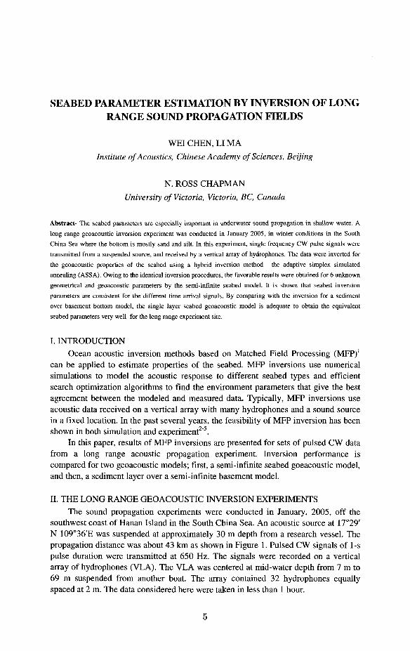
SEABED PARAMETER ESTIMATION BY INVERSION OF LONG RANGE SOUND PROPAGATION FIELDS
WEI CHEN, LI MA
Institute of Acoustics, Chinese Academy of Sciences, Beijing
N. ROSS CHAPMAN
University of Victoria, Victoria, BC, Canada
Abstract- The seabed parameters are especially important in underwater sound propagation in shallow water. A
long range geoacoustic inversion experiment was conducted in January 2005, in winter conditions in the South
China Sea where the bottom is mostly sand and silt. In this experiment, single frequency CW pulse signals were
transmitted from a suspended source, and received by a vertical array of hydrophones. The data were inverted for
the geoacoustic properties of the seabed using a hybrid inversion method—the adaptive simplex simulated
annealing (ASSA). Owing to the identical inversion procedures, the favorable results were obtained for 6 unknown
geometrical and geoacoustic parameters by the semi-infinite seabed model. It is shown that seabed inversion
parameters are consistent for the different time arrival signals. By comparing with the inversion for a sediment
over basement bottom model, the single layer seabed geoacoustic model is adequate to obtain the equivalent
seabed parameters very well for the long range experiment site.
I. INTRODUCTION Ocean acoustic inversion methods based on Matched Field Processing (MFP)1
can be applied to estimate properties of the seabed. MFP inversions use numerical simulations to model the acoustic response to different seabed types and efficient search optimization algorithms to find the environment parameters that give the best agreement between the modeled and measured data. Typically, MFP inversions use acoustic data received on a vertical array with many hydrophones and a sound source in a fixed location. In the past several years, the feasibility of MFP inversion has been shown in both simulation and experiment2"5.
In this paper, results of MFP inversions are presented for sets of pulsed CW data from a long range acoustic propagation experiment. Inversion performance is compared for two geoacoustic models; first, a semi-infinite seabed goeacoustic model, and then, a sediment layer over a semi-infinite basement model.
II. THE LONG RANGE GEOACOUSTIC INVERSION EXPERIMENTS The sound propagation experiments were conducted in January, 2005, off the
southwest coast of Hanan Island in the South China Sea. An acoustic source at 17°29' N 109°36'E was suspended at approximately 30 m depth from a research vessel. The propagation distance was about 43 km as shown in Figure 1. Pulsed CW signals of 1-s pulse duration were transmitted at 650 Hz. The signals were recorded on a vertical array of hydrophones (VLA). The VLA was centered at mid-water depth from 7 m to 69 m suspended from another boat. The array contained 32 hydrophones equally spaced at 2 m. The data considered here were taken in less than 1 hour.
5

6
I- M !•• I- K •• I '
17.8TSrl , m T|i7.STsr
i Sainue • I 4TM r i N i
1 < i - . i •' 1 1 « - ; - i i •• 1 1 1 > _• l •
Fig. 1. Long range inversion experimental area showing the source and vertical array positions.
The stationary sound speed profiles in the water were determined from conductivity temperature-depth (CTD) measurements. The sound speed in water layer varied little from 1529.2 m/s to 1530.3 m/s, as shown in the two sound speed profiles in Fig. 2. The very weak gradient is due to the nearly constant sea water temperature in the winter season. In this experiment, the signal strength of the 650-Hz CW pulse signal was strong (signal-to-noise ratio about 8 dB) at the distance of 43 km. Several pulses were recorded for geoacoustic inversion, as shown in Fig. 3, and three were used separately for geoacoustic inversion.
: : \\ 1 2005-01-1815:00 I -: - : - f—-| 2005-01-18 17 00 | -
1 #4=
0.02|j J
Am
plitu
de
1 o
5
-0.02[l
Channel 28#(15m)
;; ,, | j ,
HHHHH|n|pM|Pfl
I'f M I I | F:
raw signal
. I j , . , j j . -j
1525 1527 1529 1531 1533 Sound speed(nVs|
.5353 8.5357
Fig. 2. The stationary sound speed profiles. Fig. 3. 650-Hz CW Pulse signal received by
the 28th hydrophone of the VLA at 43 km range.
III. GEO-ACOUSTIC INVERSION METHOD The geoacoustic inversion process for estimating the seabed properties consists
of the following: Assume a reasonable geoacoustic model to describe the interaction with the sea bottom. Select a numerical propagation method to compute the forward acoustic field. Consider an appropriate objective function as a criterion to quantify the agreement between measured and simulated data. Select an efficient optimization algorithm to search for the set of environmental parameters which produces the lowest objective function value.

7
A. The geo-acoustic model
We consider two kinds of geoacoustic models for the long-range inversion. First, a
water layer over fluid half-space seabed is chosen, (Model 1). In this model six
parameters are unknown, including three geometric parameters (water depth, D,
source range and depth, r and z), and three geoacoustic parameters of the bottom:
compressional speed c, density p and attenuation a. A fluid thin layer over the half-
space bottom was also used for a geoacoustic model, i.e., Model 2. In this model the
sound speed in the sediment is assumed to vary linearly with depth, whereas it is
taken to be depth independent in the half-space bottom. The density and attenuation
are assumed depth independent within each layer. Eleven parameters are unknown, as
shown in Fig 4 (right). For inversions of the long-range experimental data, Table 1
lists each of the unknown parameters and their search intervals. The ocean sound
speed profile and sensor positions were considered known in the inversions with both
models.
C^ID+t i ^?
Fig. 4 Two kinds of geoacoustic models, Model 1 (left) and Model 2 (right).
Table 1. Inversion parameters, labels and search intervals in Semi-infinite Seabed Model 1.
Parameters Description
S ouice range (km)
S ouice depth (m)
Water depth change (m)
S ediment s peed (mis)
S ediment attenuation (dB/1)
S ediment dens ity ( g / m )
Label
«TL
Z*f$u
D
Pssd
<*>*
pt*
Search Interval
40-46
2D-40
80-100
1600-1800
1.4-2.0
0.05-1

8
Table 2. Inversion parameters, labels and search intervals in two-layered Seabed Model 2. Parameters Description
S ounce range (km)
S ouice depth (m)
Water depth change (m)
Sediment speed (m/s)
S edimentspeed bottom (m/s)
Sediment thickness (m)
S ediment attenuation (dBA)
S ediment density ( g/flS )
Basement speed (m/s)
Basement attenuation(dB^V)
Basement density ( g / / « 3 )
Label
ten
^f&U
D
Csed
<^d(lH-h(ll)
h 5
a*
M
t d
>a
ai
chsp
hsp
^hsp
Search Interval
40-46
2D-40
aD-IDD
1500-1600
1600-1800
2-30
0.05-1
1.4-1.85
1600-1800
0.05-1
1.7-2.1
B. The forward propagation model The forward propagation model used to compute the replica pressure fields was the normal-mode model KRAKENC6.
C. The objective function The objective function, E, which is minimized by the search algorithm, consists of the normalized Bartlett processor mismatch
I » I2
\P • P{m)\ E(m) = \-\-i L
\P\ \p(m)\ where p represents the measured acoustic field data (complex acoustic pressure) and p(m) is the modeled or replica field. The model vector m={/n,}, i=l,2,...n. The symbol * indicates the complex conjugation operation. This objective function E is normalized and always produces 0 <E<\ (where a perfect match yields E = 0).
D. The search algorithm In this paper, an adaptive simplex simulated annealing (ASSA) algorithm is used for the inversions. The ASSA algorithm combines simulated annealing (SA) and the downhill simplex method (DHS) in an adaptive manner. SA is a global search involving random perturbations of the unknown model parameters. However, random perturbations that neglect gradient information are inefficient for correlated parameter spaces. Alternatively, the DHS method is a local method that retains a memory of the best models encountered in its search; combining this method with SA in a hybrid algorithm effectively provides the required memory. The result is that, as a hybrid inversion ASSA is both simpler and significantly more efficient and effective than an earlier, non-adaptive version of the algorithm. More detail about the ASSA algorithm is reported by Dosso et al.7

9
IV. INVERSION RESULTS The sound field data from three CW pulse signals: No. 9 pulse, No. 16 pulse and
No. 26 pulse, were used in the inversions. The estimated values of the six unknown parameters for the semi-infinite seabed model are listed in Table 3. The estimated values of each pulse inversion are very similar to those of the other two, except the attenuation coefficient of the second pulse The estimate for source range is in excellent agreement with the measured value of 43 km that was determined in the experiment using a differential global positioning system. Source depth was estimated with an accuracy less than 5 m of the true source depth (verified by a depth sensor TD on the source body). The sea maps showing the seabed type indicate a surface sand layer throughout the experimental area. The inverted values for the geoacoustic properties of the sediment are consistent with those for a silty sand type bottom reported by Hamilton.8
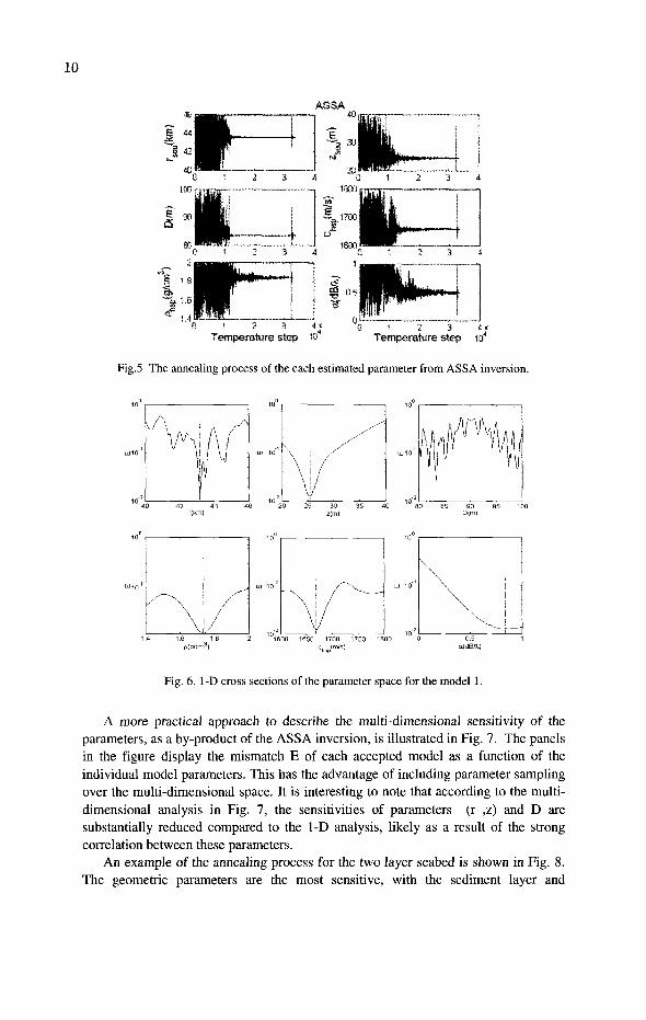
An example of the annealing process is illustrated in Fig. 5. The annealing schedule consisted of an initial temperature of 0.3 and a temperature reduction factor of 0.99, with five perturbations at each of the approximately 36000 temperature steps prior to quenching. Stable estimates are obtained for all parameters, including the low-sensitive parameters such as density and attenuation. The high-sensitive geometric parameters, source range and depth, are determined to a low-energy near the known (true) values very early in the annealing process. Fig. 6 shows the one-dimensional (1-D) cross sections of the parameter space. In each panel, the other parameters that are not varied are held fixed at their final values. This figure illustrates the features that make geoacoustic inversion a challenging problem: the 1-D cross sections exhibit multiple local minima, in this case for some of the sensitive geometrical parameters. Fig. 6 displays a wide range in parameter sensitivities (a sensitive parameter is one for which a small change in the parameter value near the minimum results in a large change in the mismatch). Source range and depth (r,z) and water depth D are the most sensitive parameters, while the others are less sensitive. Parameter sensitivities determined in this manner are commonly used to identify which parameters can be well determined by inversion. However, it should be recognized that 1-D sensitivities provide an incomplete description of the parameter space since they ignore multi-dimensional correlations.
Table 3. Geoacoustic and Geometrical parameter estimates for the inversion at source range 43 km.
Pulse 09
Pulffild
Pulse 2d
CN> M s)
1668.83
1658.08
1677.15
A * fc'*1 )
1.761
1.841
1.669
°M«tB/A)
0.839
0.493
0.644
«•«. w
43.199
43.529
42.846
f™ W
25.372
24.382
23.869
rXm)
83.539
83.409
82.928
10
ASSA
0 1 2 3 4JC
Temperature step TO 0 1 2 3 4«
Temperature step io4
Fig.5 The annealing process of the each estimated parameter from ASSA inversion.
\
/ 1.4 1 6 1 .£
p(g/cm3)
Fig. 6. 1-D cross sections of the parameter space for the model 1.
A more practical approach to describe the multi-dimensional sensitivity of the parameters, as a by-product of the ASSA inversion, is illustrated in Fig. 7. The panels in the figure display the mismatch E of each accepted model as a function of the individual model parameters. This has the advantage of including parameter sampling over the multi-dimensional space. It is interesting to note that according to the multidimensional analysis in Fig. 7, the sensitivities of parameters (r ,z) and D are substantially reduced compared to the 1-D analysis, likely as a result of the strong correlation between these parameters.
An example of the annealing process for the two layer seabed is shown in Fig. 8. The geometric parameters are the most sensitive, with the sediment layer and

11
basement half space parameters in descending order of sensitivity. The estimated values for the sensitive geometric parameters are in good agreement with the values obtained in the experiment. Comparing the estimated values for the geoacoustic parameters from the inversions with both models, we note that the estimated sediment sound speed for model 1 is roughly a mean value of the estimated sound speeds for the sediment and basement half space from Model 2.
&3
• * s l
<,&&
^3
1S.\ -.-
mm n£% t ,* *:
40 42 44 46 20 r(km)
40 80
Fig. 7. Multi-dimensional sensitivity analysis. The small dots indicate the mismatch as a function
of parameter values from ASSA inversion.
A S S A
% — ,-
• *A 1 « t
e
« «.S 1 15 ? » t,i ! U I
m « «.« ! U I
~*wm # u i u i
ftP Q
WT
e
J Temperature step x to* I £ " • E L
« M 1 « I . t U 1 U ) Temperature step x t o 1 Temperature step x to*
Fig. 8. The estimated parameters of Model 2 using the ASSA inversion.
12
The normaled sound intensity at 43 km with P09, Model 1 and ode I 2 0
10
20
30
40 E f 50 o Q
60
70
80
90
100
0 10 20 30 40 50 Sound intensity, dB
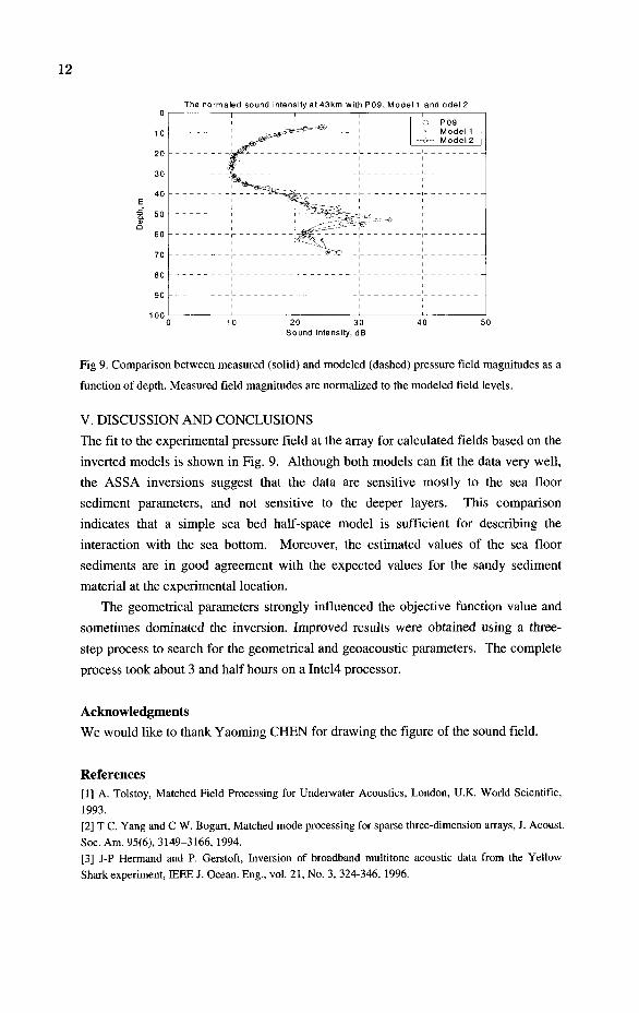
Fig 9. Comparison between measured (solid) and modeled (dashed) pressure field magnitudes as a
function of depth. Measured field magnitudes are normalized to the modeled field levels.
V. DISCUSSION AND CONCLUSIONS
The fit to the experimental pressure field at the array for calculated fields based on the
inverted models is shown in Fig. 9. Although both models can fit the data very well,
the ASSA inversions suggest that the data are sensitive mostly to the sea floor
sediment parameters, and not sensitive to the deeper layers. This comparison
indicates that a simple sea bed half-space model is sufficient for describing the
interaction with the sea bottom. Moreover, the estimated values of the sea floor
sediments are in good agreement with the expected values for the sandy sediment
material at the experimental location.
The geometrical parameters strongly influenced the objective function value and
sometimes dominated the inversion. Improved results were obtained using a three-
step process to search for the geometrical and geoacoustic parameters. The complete
process took about 3 and half hours on a Intel4 processor.
Acknowledgments We would like to thank Yaoming CHEN for drawing the figure of the sound field.
References [1] A. Tolstoy, Matched Field Processing for Underwater Acoustics, London, U.K. World Scientific,
1993.
[2] T C. Yang and C W. Bogart, Matched mode processing for sparse three-dimension arrays, J. Acoust. Soc. Am. 95(6), 3149-3166, 1994. [3] J-P Hermand and P. Gerstoft, Inversion of broadband multitone acoustic data from the Yellow Shark experiment, IEEE J. Ocean. Eng., vol. 21, No. 3, 324-346, 1996.

13
[4] L. Jaschke and N.R. Chapman, Matched field inversion of broadband data using the freeze bath method, J. Acoust. Soc. Amer., 106, 1838-1851, 1999. [5] M. Siderius, P. Nielsen and P. Gerstoft, Range dependent sea bed characterization by inversion of
acoustic data from a towed array receiver, J. Acoust. Soc. Amer., 112, 1523-1535, 2002.
[6] M.B. Porter, The KRAKEN normal mode program, SACLANTCEN Technical Report SM-245, SACLANT Undersea Research Centre, La Spezia Italy, 1991.
[7] S E. Dosso, M J. Wilmut, A S. Lapinski, An Adaptive-Hybrid Algorithm for Geoacoustic Inversion, IEEE J. Ocean. Eng., vol. 26, No. 3, 324-336, 2001.
[8] Hamilton E L. Compressional-wave attenuation in marine sediments. Geophysics, 37, 620, 1972.

HIGH RESOLUTION RADON TRANSFORM AND WAVEFIELD SEPARATION
JIANWEI CHEN
Hangzhou Institute of Geology, Hangzhou, China, 310023
QINGCHUN LI, PENG WU* and BAOWEI ZHANG Chang'an University, Xi 'an, China, 710054
*wupeng21 [email protected]
Radon transform (RT) has been widely applied in seismic data processing and interpretation, it owns fine effect in the events identification, wavefield separation, de-multiples, velocity analysis etc. This paper discusses the factors that affect the resolution of RT and the strategies for achieving the high resolution. We solve the spare matrix by the conjugate gradient [6], which does not affect the resolution and improves the computation efficiency. On the basis of the differences of velocity and intercept time between p-wave and s-wave, we separate the seismic waves by the high resolution hyperbolic RT. With theoretical models and the practical data, it makes clear that the resolution and computation efficiency of the conjugate gradient for solving the hyperbolic RT algorithm is better and more practical to separate the wavefields.
1 Introduction
Generally, we achieve wavefield separation as follows: transforming the data into a new domain, different wavefields can be separated because of their different properties in the new domain, then lining out those do not need and separating, switch the processed data to primary domain, finally we come to separate. RT is such a fine mathematic method. In recent years, linear RT (also called T — p transform) and parabolic RT
(X — q transform) are applied to wavefield separation. Because these two transforms have time-invariant property, we can implement in frequency domain, changing the problem of t-x into that of f-x and solving the local problem in each frequency composition. In linear RT domain, both reflected p-wave and converted s-wave will turn to ellipse arcs, we can separate them according to the difference of slowness and intercept. In X — q domain, the separation freedom is limited, the ellipse arcs of p-wave and s-wave being superposed, detached effect is not satisfactory, therefore this method is not practical. Parabolic RT is evolved from linear RT, only changing p to q in transform gene. It can focus the reflected event which is in form of hyperbola into almost a point, compressional wave and converted wave can easily be separated in transformed domain, and this method can be realized with fast algorithm in frequency domain, possessing certain practicability. But the time-invariant property of hyperbolic RT is approximate, and if hoped fine fruitage,, partial normal moveout correction will be required, otherwise the reflected events can not be approximated well. This method even takes advantage to eliminate multiples of great slowness time caused by NMO, but it is not stable. In order to improve separation accuracy further, we here take hyperbolic RT to implement velocity stack in t-x domain[l][2]. Theoretically, P-wave and converted s-wave with velocity difference and reflection character will focus on different points after transformation, while a set of linear wave distribute in a bit of district, easy to be separated[5] [6]. Meanwhile, high efficiency and accuracy will be achieved after applying the conjugate gradient algorithm.
15

16
2 Fundamental Principle
2.1 Principle of the hyperbolic RT
For the CSP gather, the forward transform gene is defined as hyperbolic stack, expression (1) and (2) are forward and inverse transformation of the hyperbolic Radon respectively:
d(T,q) = Y2m(t = ̂ T2 +qx2,x) (1) V
d{t,x) = 'Y^m{t = sjt2 -qx2,q) (2) V
Here X denotes geophone offset, t denotes two way time, q = yvrms , and 7
intercept time, Vrms root mean square velocity or NMO velocity.
The reflection events in CSP gather are a series of hyperbolas, since one hyperbolic event corresponds to one group of (T — q ) value, the CSP gather can be projected into
v-t pairs with forward hyperbolic RT. As a result, reflected P-wave or converted P-SV wave which has the character of hyperbolic reflected property will focus on one point in transformed domain, while the linear (refracted, direct, surface wave) waves distribute a block of region. The linear waves possessing the low velocities have big q value and can be separated clearly from q value of the reflected wave and can be eliminated easily in transformed domain, We may suppress those non-reflected wavefields easily by limiting the range of q values in transformed domain, this method can suppress multiples effectively and achieve wavefield separation.
Expression (1) written in matrix: d = Lm (3)
Where vector d contains Mt x Nx elements and m MrxNv elements, L is (Mt x Nx )x (M T x N v) dimensional operator matrix, this operator could convert one point in t - q domain into a hyperbolic event in t — X domain, supposing L be full
order operator, adjoint operator or transposed operator LF stands for NMO stack. Forward transformation can be educed by least squares method. From d=Lm, making object function minimum, we get m .
\ty = ILf - Lm 21}-> Minimize (4)
Derivate m to obtain the least-squares solution:
m = (LTL)~1 LTd = (llLYm0 (5)
m0 is low resolution velocity stack computed by transposed or adjoint operator. m is relatively high resolution result by least-squares inversion.
2.2 High resolution hyperbolic RT
Hyperbolic RT calculated by least-squares inversion method still possesses low resolution. In order to improve the transform resolution further, hyperbolic RT domain is
17
converted to sparse pulse equation, namely, solving sparse solution. For hyperbolic RT, value and constraint of sparse solution are solved in X — q domain, generally there are many standards to determine sparse property. This paper takes Cauchy class standard, make object function minimum:
7=| | r f-L»i |2+//^ln(l + mt7*) (6) k
Here mk is the element of m obtained by RT, JU and b distributed parameter
accordingly, object function derivates m, we obtain:
LTLm-LTd+Qm=0 (7)
Here Q is a diagonal matrix, the diagonal element in Q is:
& ~V7^ (8)
b+mt m may be get from (7):
m=(llL + QY LTd = (LTL + Q)~lm0 (9)
Here mo = L d is the result of low resolution RT gained by adjoint or conjugate transposed operator, namely without removing space convolution effect. Multiplying
operator IL L + QI , we get the result of high resolution RT.
mk =(LTL + Qk_ym0 (10)
Expression (8) substitutes in expression (10), we get specific solution:
2u mk= IJL + -—?—— m0 (11)
* + i»i?-iJ k is iteration times. For practical CSP trace, matrix size and amount of calculation
are very great if solving directly, when introducing conjugate gradient method, matrix L
and iJ need not to be stored, even the matrix may be omitted and operates vector
directly. One point of operator L in T —q domain corresponds to one hyperbolic
event in t — x domain, data along hyperbolic trajectory in t — x domain is scanned
and stacked into a series of points by operator L . Given primary problem:
y — Lx, x' = L y,taking conjugate gradient method to solve min\ |Lx— v|| \, to over-
determined problem we give least squares method solution, to under-determined problem
we give least norm solution.
2.3 Conjugate gradient (CG) algorithm
CG algorithm is also called conjugate inclined survey method, it is an orthogonal projection method, its convergence is assured and processing procedure needs very limited work space only, iterative operand is also very limited each time and matrix multiplying or dividing can be avoided, which make it compute rapidly and efficiently.
18
Let b replace y, A replace L ,so y = Lx becomes b = Ax , the following three steps describe the procedure of CG algorithm:
Take arbitrarily *'0' e Rn
Let r®=b-Ax®,P®=r® While k = 0 ,1 , . . . , do iterations:
(r(k)yk))
x'k+l)=x(k)+akp{k)
r(*+D = r(*> -akAp(k)
(r{k+l),r(k+i)) A = ( r ( * \ r ( t ) )
/,<*+I>=r (k+1)+&/,<*>
If r W = 0 or (p(*),Ajp'*)j = 0 , the algorithm stopped, If residual vector
(/>W,ApW) = 0 , let JCW=JC*. If (pW,ApW)=0 , we have p W = 0 , namely
(/•(*),rWj = (rW,pWj = 0, and rW = 0 , since A is forward defined. Obviously, the
problem with n equations can be solved with CG method by n steps theoretically and exact solution will be reached, It is a direct algorithm actually.
2.4 Workflow of high resolution hyperbolic RTfor wavefield separation
The following eight steps describe the Work flow of high resolution hyperbolic RT for wavefield separation
(1) Enter t-x seismic record (2) Set initial value and compute operator matrix (3) Compute initial velocity stack matrix m (4) Solve sparse linear set of equations using CG iteration method (5) Output (T-q)
(6) Discriminate and separate wavefield in {z — q)
(7) Radon inverse transformation
(8) Output seismic record having separated in t-x domain
3 Testifying of the Theoretical Models and Practical Data
3.1 Theoretical models
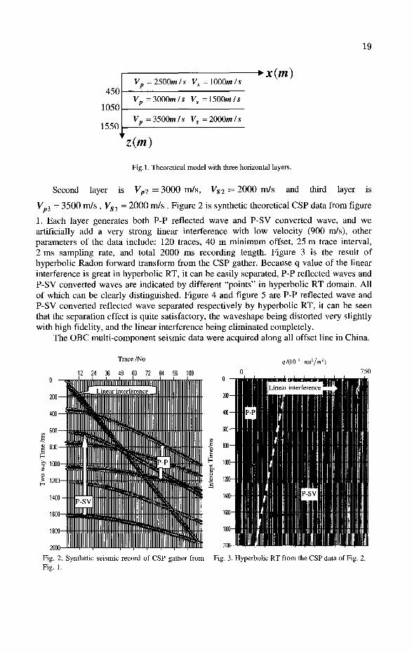
Figure 1 is a three horizontal layers geologic model. The depth of each layer is H x =
450 m, H2 = 1050 m, H3 =1550 m, P-P-wave velocity of the first layer is Vpi = 2500 m/s,
that of p-s-wave is Vsl = 1000 m/s.
19
450
1050
1550
Vp = 2500m/s Vs = 1000mIs -+x(m)
Vp = 3000mIs Vs = 1500mIs
Vp = 3500m Is Vs= 2000m /s
z(m)
Fig.l. Theoretical model with three horizontal layers.
IS Second layer is VP2 = 3000 m/s, Vs2 = 2000 m/s and third layer
Vp3 = 3500 m/s , VS3 = 2000 m/s . Figure 2 is synthetic theoretical CSP data from figure
1. Each layer generates both P-P reflected wave and P-SV converted wave, and we artificially add a very strong linear interference with low velocity (900 m/s), other parameters of the data include: 120 traces, 40 m minimum offset, 25 m trace interval, 2 ms sampling rate, and total 2000 ms recording length. Figure 3 is the result of hyperbolic Radon forward transform from the CSP gather. Because q value of the linear interference is great in hyperbolic RT, it can be easily separated, P-P reflected waves and P-SV converted waves are indicated by different "points" in hyperbolic RT domain. All of which can be clearly distinguished. Figure 4 and figure 5 are P-P reflected wave and P-SV converted reflected wave separated respectively by hyperbolic RT, it can be seen that the separation effect is quite satisfactory, the waveshape being distorted very slightly with high fidelity, and the linear interference being eliminated completely.
The OBC multi-component seismic data were acquired along all offset line in China.
Trace /No
12 24 36 48 60 72 84 96 108 750
Fig. 2. Synthetic seismic record of CSP gather from Fig. 3. Hyperbolic RT from the CSP data of Fig. 2. Fig. 1.

20
T r a c e / N o
12 24 36 48 60 72 84 96 108
0 -
200-
400-
600-
T r a c e / N o
10 20 30 40 50 60 70
Fig.4. P-P reflected wave separated by hyperbolic RT. Fig.5. P-SV reflected wave separated by hyperbolic RT.
3.2 Practical data
Seismic exploration data picked up by multi-component in sea domain. Figure 6 is time stacked section of the vertical component. Figure 7 is the section after adding hyperbolic RT in processing. Compared Fig. 7 with Fig. 6, we can see that the resolution get higher obviously at 600ms, 1500ms, 2000ms, and the resolution is higher obviously, especially within the three ellipses in Fig. 7.
I
CDP/No
Fig.6. Time stacked section before RT (OBC data, z component).

21
CDP/N
Fig.7. Time stacked section after RT, P-SV converted wave of z component has been suppressed the resolution has been improved. Such as the three ellipses I, II, III.
4 Conclusions
With theoretical models and practical data, we get the concluded remarks, hyperbolic RT is a wavefield separation method which can keep true energy and owns high
resolution, owing to t0 and q are different in different wavefields, they can be easily
separated in the transformed domain, and this method has the characters as follows: (1) Noises can be eliminated simultaneously when separating wavefields, non-
reflected interferential signals can be suppressed. (2) Not only reflected p-wave can be separated, so can be done to converted waves
and multiples. (3) Keep energy fidelity in processing. Because each trace ^transformed domain corresponds to determined stack velocity,
velocity can be analyzed when we take wavefield separation in transformation. Reflected waves are completely focused in transformed domain, so imaging can be done directly in transformed domain and needs not to be transformed into t-x domain.
Reference
1. Q. Li, High Resolution Hyperbolic RT Multiple Removal, The University of Alberta, 2001.
2. Y. X. Liu and Mauricio D.Sacchi, De-multiple via a Fast Least-squares methods Hyperbolic RT, SEG IntT Exposition and 72nd Annual Meeting, 2002.

22
3. Q. S. Cheng, Mathematical Principle of Digital Signal Processing, Petroleum Industry Press (1982).
4. S. Y. Xu, Wavefield separation with T — q transform method, China Offshore Oil and Gas (Geology) 13(5) (1999) 334-337.
5. X. Y. Sun, The separation of P- and S-wave fields using X — q transform method, Petroleum Geology & Oilfield Development in Daqing 21(4) (2002) 76-79.
6. X. W. Liu, High resolution Radon transform and its application in seismic signal processing, Progress in Geophysics 19(1) (2004) 8-15.

THREE-DIMENSIONAL ACOUSTIC SIMULATION ON ACOUSTIC SCATTERING BY NONLINEAR INTERNAL WAVE IN COASTAL OCEAN
LINUS Y. S. CHIU, CHI-FANG CHEN
Department of Engineering Science and Ocean Engineering, National Taiwan University E-mail: cvs(3),uwaclab. na. ntu. edu. tw
JAMES F. LYNCH
Woods Hole Oceanography Institute
Nonlinear internal wave (NIW) packets cause ducting and whispering gallery effects in acoustic propagation. The acoustic energy restricted within the internal wave crests (crest-crest) on the shelf is the ducting effect, and the energy confined along the crest when the source is located upslope from the NIW crest is the whispering gallery effect. This paper presents the simulation results concerning the phenomena of whispering gallery by FOR3D wide-angle version. It appears that energy emerges right before and along the wave crest and then vanish right in the back of the wave crest and then converges again, especially with the lower frequency band (150Hz~ 600Hz).
1 Introduction
The influence on the amplitude and phase of an acoustic field propagating through the shallow water waveguides is significant over relatively short ranges while the sound speed fluctuations in the region are typically less than one percent of the mean speed [1-5]. Our interest in this behavior stems from two points related to underwater communication system or the sonar performance. It is that signal detection is a function of the signal-to-noise ratio and is affected by transmission loss (TL) variability caused by sound speed perturbations with internal wave.
Recent papers and experiments address the acoustic field is fluctuated by the nonlinear internal waves (NIW). We have seen the energy distribution has specified modification due to the acoustic mode coupling while the sound propagates across the internal wave. They also cause ducting and whispering gallery effects as the sound propagates along the internal waves. The acoustic energy restricted within the internal wave crests (crest-crest) is the ducting effect [6], and the energy confined along the crest when the source is located at the upslope region relatives to the NIW crest is called the whispering gallery effect.
Computer simulation offers a practical method for systematic assessment of TL and coherence degradation in complex ocean environments. This approach is applied here, where the TL and azimuthal spatial coherence are estimated for frequencies band of 50-800 Hz as a function of range, depth, and azimuth in shallow water, continental shelf environment under summer condition. Sound speed fluctuations considered in this paper are induced by an internal gravity wave field that perturbs the thermocline. Some recent theoretical efforts have considered the effect of internal wave induced phase decorrelation on horizontal arrays in both deep and shallow water environments under a variety of modeling assumptions [6].
Our analysis differs from those of previous studies in that we employ a simplified, data-constrained internal wave model which is observed in the ASIAEX experiment, South China Sea (SCS) component that includes a azimuthal anisotropic component, and
23

24
apply 3D acoustic modeling techniques (FOR3D with wide angle version) to estimate TL and azimuthal coherence in this environment.
This paper presents evidence that acoustic field can be significantly affected in an environment supporting oceanographic features that break azimuthal symmetry. Such affection might not be predicted by N x2D calculations since they ignore horizontal refraction and may thus produce misleading TL and azimuthal coherence in these environments. This paper also addresses and quantifies the whispering Gallery Effect induced by the internal solitary wave in the typical continental slope region. We have two basic results: 1. Enhanced energy emerges right before and along the wave crest and then vanishes
right in the back of the wave crest and then converges again, especially with the lower frequency band (150Hz~ 600Hz).
2. Scattering of sound due to the internal solitary waves brings about much worse azimuthal coherence in the time scale of 25 minutes. The azimuthal coherence is better in lower frequencies and increasing depth.
In Sec. II we briefly review the simulation scenario and analysis approach. In Sec. Ill, we give the results and implementation of numerical experiments, which estimate energy distribution in the 3D field, the adaptive depth-averaged acoustic energy and azimuthal coherence under several conditions. The summary and conclusions are presented in Sec. IV.
2 Simulation Approach
Three dimensional effects on underwater acoustic propagation have been frequently reported [7-9]. The acoustic propagation model is based on the 3D parabolic approximation to the Helmholtz equation implemented in the computer code FOR3D [9]. This code implements a finite difference solution scheme, using discretized differential operators to represent wide-angle propagation in elevation and narrow-angle azimuthal coupling. The major causes for the 3D effects are variations in azimuth of bottom topography and/or water column properties [10-13]. Experiment site in South China Sea is of a similar nature, in that both bathymetry and horizontally anisotropic water column properties contribute to horizontal refraction of energy.
Details of the simulation scenario and parameters are given in the Fig.l (a). The acoustic point source which placed in the upper water column is assumed to be a tow acoustic source. The emitted sound propagates in the wedge bathymetry which slope is equal to the 1/20. Superimposed on the sound speed volume is an observed internal wave in South China Sea which causes very large thermocline depressions even to 85 meters from thermo. Internal wave propagated onshore from 2 kilometers far from the source until the 0.5 kilometers. The dynamic elevations of the internal wave due to the onshore-propagating are ignored in this time scale of only 25 minutes. Finally the bottom parameters are constant in range and selected from a somewhat very hard, sandy bottom. And the density is set to be twice that of the water density.
2.1 Transmission loss
Nonlinear internal wave fields introduce significant azimuthal transfer of energy. Acoustic field calculations performed through a set of 2D range/depth planes (a.k.a. Nx2D computations) for different azimuthal directions allow for variations in sound speed within range/depth planes but ignore horizontal refraction of energy between adjacent

25
planes. The 3D calculations presented here include such azimuthal coupling, if present, and can be used to assess the relative importance of horizontal refraction in complex oceanographic environments. A rather simple means of estimating the amount of azimuthal energy transfer is outlined here and used to interpret TL and coherence results. Define a adaptive depth-averaged acoustic energy density (ADAAE) E:
E = E{r,$)
) \u\ I p(z)dz
C,H (1)
where H is the total depth(or arbitrary depth) of water column and sediment, and c 0 is a
nominal reference sound speed. The depth averaged, or mean TL, 7Xz([l] and [4]), is TLZ =10 1og10£ where E has unit of energy per area.
(2)
/ ^ ^ ' 8 km ~~~~~\
U 2 km
: \n/v 1.2 km j
400m L i
Source Depth
Slope
Frequency
dr
dz
e d G
Amplitude of I W s
(from thermalcline)
Ave. Phase speed of I W s
IW's propagating timing
= 20m
- 1 / 2 0
- 50-800 Hz
= A/10
= A/10
- 180'
= 1"
= 85 meters
= 0.8 m/s
= 25 min.
BHtt!
(a)
I W s
(b)
Figure 1. The details of simulation scenario and parameters. Internal wave propagated onshore from 2 kilometers far from the source until the 0.5 kilometers.
2.2 Azimuthal Coherence
Azimuthal coherence is a three-dimensional function which includes the parameters r, z, P (range, depth and azimuth). The complex pressure field U (r, z, /?) (azimuthally

26
across the slope) is correlated with its value at j3 = 0 (along the slope) and temporally averaged and then normalized as:
C^^P)-u(r,z,9(f)u(r,z,JJ))\
(3) ^|M(r,z,90f)|2J}(| u{r,z,P)
See also Fig.l (b). The angle brackets represent the time average over environment snapshot (-25 minutes). This dependence on integration time is due to the non-stationary nature of the sound speed filed induced by the internal waves.
3 Implementation and Results
3.1 Results of Transmission loss
This section presents some results of acoustic calculations for TL, ADAAE, effect of whispering gallery and azimuthal coherence. TL examples presented here are the single environment snapshot while the internal wave is right at 1 km from source and the frequencies are of 50 Hz and 150 Hz. They are shown in Fig.2 (a), (b) as a function of range and azimuth at specified depth. ((a)30 meters, (b)50 meters). The first column in each figure is the case for imposed internal wave; the middle is the case for background sound speed profile (without the internal wave) and the last is the difference between the previous two columns.
In (a) and (b), the middle ones are the typical bench mark of three-dimensional wedge problem. Clear see that energy distribution is no longer circle-like but curved and bend down to the deeper water region. But the internal wave comes in (propagates onshore), they may induce the oceanic waveguide so as to concentrate the energy near or along the boundary, as shown in the left column of Fig. 2. Such concentration of energy near the boundary is completely analogous to the whispering gallery modes. The right column in Fig. 2 shows the enhanced horizontal refraction induced by the internal wave since the phasing and the amplitude of the interference pattern has changed.
SOHz S ! S l I 150Hz I
1 I

27
(b)
Figure 2 Transmission losses at specified depths, ((a) 30 meters, (b) 50 meters). The left columns show the case of incoming internal wave; the middle ones are the cases of background sound speed profile and the right ones are the differences.
3.2 Results ofADAAE
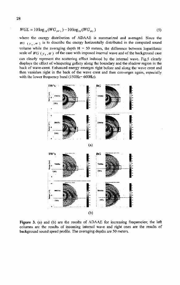
In order to clearly see the redistribution of energy caused by the internal wave, the ADAAE is utilized where H = 50 meters and shown in Fig. 3. The averaging depth of 50 meters is chosen to see the acoustic scattering of upper water column induced by the incoming internal wave. Fig. 3(a) and (b) are the cases for increasing frequencies; the cases for the incoming internal wave are shown in the left column and the ones for the background sound speed profile are shown in the right column. Only the results of 150Hz, 200Hz, 700Hz and 800Hz are shown here. Fig.3 illustrates the enhanced energy occurring near and along the boundary which is regarded as the oceanic waveguide induced by the nonlinear internal wave, especially in Fig. 3(a). For lower frequencies (50-600Hz), the modal interference pattern of energy and the scattering effect are clearly seen since the source may excite only lower modes, but the pattern are getting disordered (see Fig.3. (b)) due to the higher modes excited at higher frequencies. The effect of enhanced energy along the boundary of the internal wave has been gradually smeared (not shown here) while the averaging depth is increasing. This tells that the whispering gallery effect mainly occurs in the upper water column so that the effect is smeared with the increasing averaging depth.
3.3 The Effect of Whispering Gallery
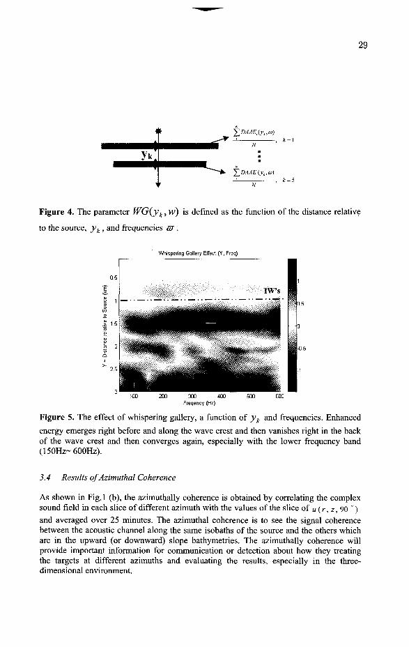
The quantity has been defined for describing the effect of whispering gallery since the enhanced energy is horizontally stratified induced by the internal wave. The parameter WG (y k, w) is defined as the function of the distance relative to the source, yk , and frequencies G7, see also Fig. 4.
f^DAAE&^m) WG(yk,m) = ^ , * = 1,2,3,... (4)
N
28
PFGL = 101og 1 0 (^G / ^) -101og 1 0 (^G S G ) (5)
where the energy distribution of ADAAE is summarized and averaged. Since the WG (yk,m ) is t 0 describe the energy horizontally distributed in the computed sound
volume while the averaging depth H = 50 meters, the difference between logarithmic scale of WG (yt,m) of the case with imposed internal wave and of the background case
can clearly represent the scattering effect induced by the internal wave. Fig.5 clearly displays the effect of whispering gallery along the boundary and the shadow region in the back of wave-crest. Enhanced energy emerges right before and along the wave crest and then vanishes right in the back of the wave crest and then converges again, especially with the lower frequency band (150Hz~ 600Hz).
IW's I far-
I BG
(a)
IW's
? ° i&» I BG
i750Hz5pfcV
-§ 800Hz £
*$$£] fc I ?Jq£
i
(b)
Figure 3. (a) and (b) are the results of ADAAE for increasing frequencies; the left columns are the results of incoming internal wave and right ones are the results of background sound speed profile. The averaging depths are 50 meters.
29
y*
£M£,(V„(»)
%DAAE,(yk,co)
-, * = 5
Figure 4. The parameter WG{yk, w) is defined as the function of the distance relative
to the source, yk , and frequencies XU .
Whispering Gallery Effect (Y, Freq)
Freqency (Hz)
Figure 5. The effect of whispering gallery, a function of yk and frequencies. Enhanced
energy emerges right before and along the wave crest and then vanishes right in the back of the wave crest and then converges again, especially with the lower frequency band (150Hz~600Hz).
3.4 Results of Azimuthal Coherence
As shown in Fig. 1 (b), the azimuthally coherence is obtained by correlating the complex sound field in each slice of different azimuth with the values of the slice of u (r, z, 90 ") and averaged over 25 minutes. The azimuthal coherence is to see the signal coherence between the acoustic channel along the same isobaths of the source and the others which are in the upward (or downward) slope bathymetries. The azimuthally coherence will provide important information for communication or detection about how they treating the targets at different azimuths and evaluating the results, especially in the three-dimensional environment.

30
Fig. 6(a) and 6(b) show the cSw(r<z<P) results of at z = 20 meters and 50
meters with different frequencies. Scattering of sound due to the internal solitary waves brings about the worse azimuthal coherence especially with higher frequencies. Compare the cases between different frequencies in Fig. 6(a) or 6(b), azimuthal coherence is better with lower frequency (even to 0.6 differences at specified range and azimuth) since higher modes excited by high frequencies may cause the disordered interference pattern so that the phasing and the amplitude of the modes would be highly disturbed. This arises the worse azimuthal coherence in higher frequencies. On the other hand, the scattering effect mainly occurs in the upper water column, this may bring about the high coherence in the deeper water (0.6~0.7 difference at deeper water column). Compare Fig. 6(a) with 6(b), the coherence is much better with increasing depth, which is also due to the downward refracting sound speed profiles. This causes that the energy is transferred from high sound speed regions to low sound speed regions so that the deeper water column had higher coherence.
150Hz
400Hz
200Hz
800Hz
(a)
150Hz
400Hz
20011z
800Hz
I
\
(b)
Figure 6. The results of Q (r,z,B) a t 20 meters (a) and 50 meters (b) with different
frequencies. Azimuthal coherence is better with lower frequency and with increasing depth.

31
4 Summary and Conclusions
This paper describes results of fully 3D numerical experiment involving the acoustic wave fields through a dynamic, 3D oceanographic environment in a typical continental slope region. The environments consists of both dominate summer sound speed profile and the observed internal wave in South China Sea which causes strongly thermocline depressions. A fully 3D parabolic code (FOR3D) with wide angle version is used to compute the transmission loss in the band from 50Hz to 800Hz, the adaptive depth average acoustical energy and the azimuth coherence which is the time-dependent function. The internal wave in the continental slope brings about the enhanced energy emerging along or near the wave since the wave crest induces the oceanic waveguide.
Such concentration of energy near the boundary is completely analogous to the whispering gallery modes. The simulation reveals that the space-time structure of an acoustic field can be significantly altered in this type of oceanographic environment for some propagation conditions. This would not be predicted on the basis of 2D or Nx2D calculations since those calculations ignore the azimuthally coupling.
ADAAE is utilized to clearly see the redistribution of energy caused by the internal wave but not only choose one specified depth. The effect of enhanced energy along the boundary of the internal wave has been gradually smeared (not shown here) while the averaging depth is increasing. This tells that the effect of the whispering gallery or the scattering by the internal wave mainly occurs in the upper water column so that the effect is smeared with increasing the averaging depth. The parameter wG (y k, w) clearly displays the effect of whispering gallery along the boundary and the shadow region in the back of wave-crest. Enhanced energy emerges right before and along the wave crest and then vanishes right in the back of the wave crest and then converges again, especially with the lower frequency band (150Hz~ 600Hz). Azimuthal coherence estimated as a function of time-dependence is better in the lower frequencies ( gained from 0.35 even to the 0.95 in the frequency of 150Hz and 800Hz at specified range, depth and azimuth) and also with increasing depth.(0.6~0.7 difference at deeper water column).
5 Reference
1. J. Lynch, S. Ramp, C. S. Chiu, T. Y. Tang, Y. J. Yang, and J. Simmen, "Research highlights from the Asian Seas International Acoustics Experiment in the South China Sea," IEEE J. Oceanic Eng., vol. 29, pp. 1067-1074, Oct. 2004.
2. C. S. Chiu, S. Ramp, C. Miller, J. Lynch, T. Duda, and T. Y. Tang, "Acoustic intensity fluctuations induced by South China Sea internal tides and solitons," IEEE J. Oceanic Eng., vol. 29, pp. 1249-1263, Oct. 2004.
3. T. Duda, J. Lynch, A. Newhall, L. Wu, and C. S. Chiu, "Fluctuation of 400-Hz sound intensity in the 2001 ASIAEX South China Sea Experiment," IEEE J. Oceanic Eng., vol. 29, pp. 1264-1279, Oct. 2004.
4. S. Finette, M. H. Orr, A. Turgut, J. Apel, M. Badiey, C. S. Chiu, R. H. Headrick, J. N. Kemp, J. F. Lynch, A. E. Newhall, K. von der Heydt, B. Pasewark, S. N. Wolf, and D. Tielbuerger, "Acoustic field variability induced by time-evolving internal wave fields," J. Acoust. Soc. Am., vol. 108, pp. 957-972, 2000.
5. D. Rubenstein, "Observations of cnoidal internal waves and their effect on acoustic propagation in shallow water," IEEE J. Oceanic Eng., vol. 24, pp. 346-357, 1999.

32
6. R. Oba and S. Finette, "Acoustic propagation through anisotropic internal wave fields: TL, cross-range coherence, and horizontal refraction," J. Acoust. Soc. Am., vol. I l l , issue 2, pp. 769-784, 2002.
7. G. Botseas, D. Lee, and D. King, "FOR3D: A computer model for solving the LSS three-dimensional, wide angle wave equation," Naval Underwater Systems Center, TR7943, 1987.
8. A. Tolstoy, "3-D Propagation Issues and Models," J. Comput. Acoust., vol. 4, no. 3, pp. 243-271, 1996.
9. D. Lee and M. H. Schultz, "Numerical Ocean Acoustic Propagation in Three Dimensions, " Singapore: World Scientific, 1995, pp. 138-144.
10. S. Finette and R. Oba, "Horizontal array beamforming in an azimuthally anisotropic internal wave field,"/. Acoust. Soc. Am., vol.114, pp. 131-144, 2003.
11. K.B. Smith, C.W. Miller, A.F. D'Agostino et al., "Three-dimensional propagation effects near the mid-Atlantic Bight shelf break (L)," J. Acoust. Soc. Am., vol. 112, issue 2, pp. 373-376, 2002.
12. C. F. Chen and J. J. Lin, "Three Dimensional Effect on Acoustic Transmission in Taiwan's Northeastern Sea," Proceedings of International Shallow-Water Acoustics, Beijing, 1997.
13. C. F. Chen, J. J. Lin and T. Lee, "Acoustic transmission of Taiwan's northeast sea," Acta Oceanographica Taiwanica, no.34, pp.39-51, 1995.

ESTIMATION OF SHEAR WAVE VELOCITY IN SEAFLOOR SEDIMENT BY SEISMO-ACOUSTIC INTERFACE WAVES: A CASE STUDY FOR
GEOTECHNICAL APPLICATION
HEFENG DONG, JENS M. HOVEM
Acoustic Research Center, Norwegian University of Science and Technology (NTNU) N-7491 Trondheim, Norway E-mail: [email protected]
SVEIN ARNE FRIVIK
WesternGeco Oslo Technology Center, Solbraveien 23, Pbox 234, N-1383 Asker, Norway
E-mail: sfrivik(3)slb. com
Estimates of shear wave velocity profiles in seafloor sediments can be obtained from inversion of measured dispersion relations of seismo-acoustic interface waves propagating along the seabed. The interface wave velocity is directly related to shear wave velocity with value of between 87-96% of the shear wave velocity, dependent on the Poission ratio of the sediments. In this paper we present two different techniques to determine the dispersion relation: a single-sensor method used to determine group velocity and a multi-sensor method used to determine the phase velocity of the interface wave. An inversion technique is used to determine shear wave velocity versus depth and it is based on singular value decomposition and regularization theory. The technique is applied to data acquired at Steinbaen outside Horten in the Oslofjorden (Norway) and compared with the result from independent core measurements taken at the same location. The results show good agreement between the two ways of determining shear wave velocity.
1 Introduction
The structure and composition of the seabed's structure are very important for many applications. For evaluation of long range sonar performance it is necessary to have precise information about the layered structure of the seabed with the densities, sound speeds and attenuations.
Quantitative characterization of the upper part of the seabed is also of major importance in both for the geotechnical and offshore industry. To reduce the risk and cost associated to sea-bottom installations such as communication cables, gas/oil cables and underwater constructions, precise and reliable information about the seafloor is needed. For this purpose it is important to know the seismo-acoustic parameters such as compressional P-wave and shear S-wave velocity, density and attenuation as function of depth. Shear wave velocity is in this context unique since it is related to shear strength of the sediments and hence used to evaluate how much load the seabed can support.
In some cases the geoacoustic properties can be acquired by in-situ measurement, or by taking samples of the bottom material with subsequent measurement in laboratories. In practice this direct approach is often not sufficient and will have to be supplemented by information acquired by remote measurement techniques in order to have the area coverage and the depth resolution required.
A possible approach for measuring the seabed's shear wave structure is to use seismo-acoustic interface waves, also known as Rayleigh, Stoneley, or Scholte waves, that may exist at an interface between two media, at least one of which must be a solid.
33

34
References to this technique are the papers by Caiti, Stoll and Akal [2], Jensen and Schmidt [7] and Rauch [11].
A general property of interface waves is that they propagate along the interface with a velocity that is closely related to the shear wave velocity. The phase velocity of an interface wave in a homogeneous solid half-space is dominated by the shear wave velocity vs. and varies from 0.87 v, to 0.96 vs, depending on the Poission ratio of the medium. The amplitude decays exponentially with distance away from the interface; the penetration is typically at the order of one wavelength [12]. If the shear wave velocity varies with depth in the bottom, which is normally this case, the interface wave velocity becomes dependent on the frequency, i.e. the interface waves are in general dispersive and the dispersion is given by the shear velocity profile of the bottom.
The objective of the study reported in this paper is to compare the shear wave velocity values obtained by analyzing the dispersion characteristics of recorded interface waves, and to compare these results with the results using common geotechnical techniques. Therefore we conducted, in 1998, a joint seismo-acoustic and geotechnical experiment at a location called Steinbaen outside Horten in the Oslofjorden (Norway). The seismo-acoustic data was acquired by the company Geomap AS and the geotechnical investigations were done by FUGRO LTD [5, 6], both companies working under a contract with Norwegian University of Science and Technology as part of the European MAST III project ISACS.
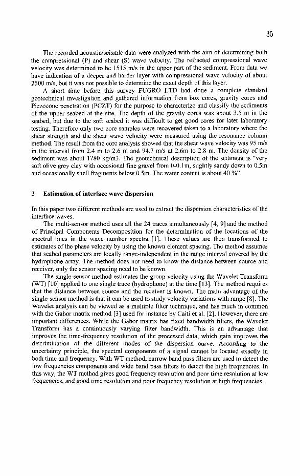
2 Data collection
In 1998 a modified refraction seismic survey was conducted by Geomap AS at Steinbaen outside Horten in Norway. The water depth at the location is 18 m. A 34.5 meter long linear hydrophone array with 24 hydrophones with spacing of 1.5 meter was used for the recording, and small dynamite charges were used as source, see figure 1. The difference between this setup and normal refraction seismic survey was that the recording length in time was increased from 1 second to 8 seconds. This was done to ensure that the seismo-acoustic interface waves were captured, due to their slow propagation speed compared to the speed of the compressional waves. The sources were set to explode approximately of 77 meter in front of receiver no 1 in the hydrophone array.
Explosive sound source 1r 1.5 m Hydrophone array
77 m ' 24 hydrophones
Figure 1. Experimental setup for reception of interface waves by a 24-hydrophone array with spacing 1.5 m situated on the seabed. The distance between source and receiver no 1 is 77 m.
35
The recorded acoustic/seismic data were analyzed with the aim of determining both the compressional (P) and shear (S) wave velocity. The refracted compressional wave velocity was determined to be 1515 m/s in the upper part of the sediment. From data we have indication of a deeper and harder layer with compressional wave velocity of about 2500 m/s, but it was not possible to determine the exact depth of this layer.
A short time before this survey FUGRO LTD had done a complete standard geotechnical investigation and gathered information from box cores, gravity cores and Piezocone penetration (PCZT) for the purpose to characterize and classify the sediments of the upper seabed at the site. The depth of the gravity cores was about 3.5 m in the seabed, but due to the soft seabed it was difficult to get good cores for later laboratory testing. Therefore only two core samples were recovered taken to a laboratory where the shear strength and the shear wave velocity were measured using the resonance column method. The result from the core analysis showed that the shear wave velocity was 95 m/s in the interval from 2.4 m to 2.6 m and 94.7 m/s at 2.6m to 2.8 m. The density of the sediment was about 1780 kg/m3. The geotechnical description of the sediment is "very soft olive grey clay with occasional fine gravel from 0-0. lm, slightly sandy down to 0.5m and occasionally shell fragments below 0.5m. The water content is about 40 %".
3 Estimation of interface wave dispersion
In this paper two different methods are used to extract the dispersion characteristics of the interface waves.
The multi-sensor method uses all the 24 traces simultaneously [4, 9] and the method of Principal Components Decomposition for the determination of the locations of the spectral lines in the wave number spectra [1]. These values are then transformed to estimates of the phase velocity by using the known element spacing. The method assumes that seabed parameters are locally range-independent in the range interval covered by the hydrophone array. The method does not need to know the distance between source and receiver, only the sensor spacing need to be known.
The single-sensor method estimates the group velocity using the Wavelet Transform (WT) [10] applied to one single trace (hydrophone) at the time [13]. The method requires that the distance between source and the receiver is known. The main advantage of the single-sensor method is that it can be used to study velocity variations with range [8]. The Wavelet analysis can be viewed as a multiple filter technique, and has much in common with the Gabor matrix method [3] used for instance by Caiti et al. [2]. However, there are important differences. While the Gabor matrix has fixed bandwidth filters, the Wavelet Transform has a continuously varying filter bandwidth. This is an advantage that improves the time-frequency resolution of the processed data, which gain improves the discrimination of the different modes of the dispersion curve. According to the uncertainty principle, the spectral components of a signal cannot be located exactly in both time and frequency. With WT method, narrow band pass filters are used to detect the low frequencies components and wide band pass filters to detect the high frequencies. In this way, the WT method gives good frequency resolution and poor time resolution at low frequencies, and good time resolution and poor frequency resolution at high frequencies.

36
4 Inversion algorithm
The inversion algorithm used in this study is a modified version of the inversion algorithm reported by Caiti et al. [2]. The main part in the inversion algorithm is the singular value decomposition (SVD) of a linear system and a forward model to determine dispersion curves from the "earth model". Assuming that the thickness and compressional wave velocity for each layer are known and with fixed parameters, the model is able to generate a group/phase velocity vector \c e R" as a function of the shear velocity vector \s
e /T :
Tv,=ye, (1)
where Jacobian J e R"x Rm. Here, m is the index over layers and n is the index over frequencies of the dispersion curve, and we will consider the most common case where m < n; that is, we have more data than estimated parameters. The solution, which is expressed as
vs=(rrr)-'rrvc (2)
minimizes ||Tvs-vc||2 in the least square sense and here || • || is the 2 norm of a vector. By
using the singular value decomposition (SVD) to the rectangular matrix T the solution can be expressed as
\s = WQT'UT\C , (3)
v.^^-^^E-1^- (4)
In equations (2) and (3) TT = W[Q 0]UT, U and W are unitary orthogonal matrices with dimension (nxn) and (mxm) respectively and Q is a square diagonal matrix of dimension m, with diagonal entries a%, called singular values of T with a>\>G>i>...>wm; O is a zero matrix with dimension (mx(n-m)); u, is the z'th column of U and w,- they'th column of W. There is an effect of ill-conditioning in the numerical solution of this inverse problem and regularization theory is used to reduce the effect with the modified normal equation
v / ={TTT + yHTHy{TT\c. (5)
where H, a square matrix with dimension (mxm), is a general operator embedding the a priori constraints imposed on the solution, and the regularization parameter y > 0. The regularized solution is given by
v ; = r f v c (6)
with r f = W(Cl + i1-'y(HW)T (HW)Yl UT (7)
In this practical case, we have used H = I, unit matrix, and hence 7* = W(Q. + jQ'[)"' UT. Figure 2 shows a flowchart of the inversion algorithm. The input data consist of the
measured dispersion curves from the previous processing described above, and the structure of an earth model. This earth model has a given number of sediment layers; the parameters are the compressional and shear wave velocities and the densities. In the

37
current application the layer thickness, here is 2 meters, the compressional velocities and the densities are fixed; only the shear wave velocities of the layers are assumed unknown at the initialization. The parameters of the earth model are inputted to a forward acoustic model (based on the scheme by Takeuchi H. et al [12]) which calculates a synthetic dispersion curve. The measured and synthetic dispersion curves are compared by an objective function, $ys) = ||7Vs-vc||
2 and the objective function is minimized by varying the free earth model parameters, in this case the shear wave velocities of the layers. This iteration is continued until an acceptable fit between the measured and the synthetic dispersion curve is obtained. The results are estimates of the shear wave velocities of the sediment layers together with an uncertainty analysis.
Initialization
' ' Adjusted
parameters i L
Measured rlisnersion curve from
analysis of the interface waves
Synthetic data by forward modeling
Feedback
' ' Objective function
4 U
No Yes Inversion
results
Figure 2. Flowchart of the inversion algorithm with five parts: initial environmental parameters' setting, acoustic forward modeling, comparison of the synthetic data computed by forward acoustic model and observed data, here the dispersion curve of the group/phase velocity extracted from the interface waves, by an objective function, minimizing the objective function by varying the environmental parameters and uncertainty analysis for inversion results, here shear wave velocity.
5 Data analysis
Figure 3 shows in the left panel the time signal traces recorded on the 24 hydrophone array from one particular shot PI-86 at the Steinbaen site. The left panel shows the raw data with the full frequency bandwidth. The middle panel shows the high pass filtered and zoomed version of the same traces, the high frequency filtering emphasizes the refracted arrivals and we can observe an refracted arrival which determines the compressional wave velocity of the upper sediment layer to approximately 1515 m/s. In the right panel the raw data have been low pass filtered, which brings out the interface waves. The amplitudes of the interface waves are weak compared to the water borne modes (compare left and right panels in Fig 3), but one can clearly observe that the velocity of the interface waves is in the range of 40 to 100 m/s
The low pass filtered versions of each of the recorded traces are used in die subsequent dispersion analysis using the time-frequency analysis of the Wavelet Transform (WT), and time is converted to velocity since the distance between source and the receiver is known. An example of the analysis of trace no 10 is shown in figure 4 as group velocity as function of frequency. Both panels show the same results but presented in two different ways. The left panel shows a colormap and in the right panel the data are plotted in contour plot. From the latter representation it is easy to detect the maximum values along the each contour as indicated by the stars in the left panel of figure 4. The detected maximum values are the samples of the dispersion curve that will be used as the measured data in the inversion algorithm of figure 2.

38
<B A
E 4
fli^lf
I
1
1 i
! 1 1 ! I
!i
1:
J [ 1 '
! 1
! ! ,
"J iffi
1 1 1
1 1
1
1 1
B °
0.05
0.1
0.15
0.2
0.25
0.3
0.35
0.4
0.45
^ 0.5 80 90 100 110 80 90 100 110
Offset from the source [m] 80 90 100 110
Figure 3. Time signal traces recorded on the 24 hydrophone array from shot Pl-86 in Steinbaen site. Left panel: The raw data with full bandwidth; Middle panel: High pass filtered traces emphasizing the refracted arrivals and Right panel: Low pass filtered traces brings out the interface wave. A simple interpretation of the middle panel indicates that the P-wave velocity of the upper part of the seabed is about 1510 m/s. The dispersion of the interface wave in the right panel indicates that the velocity of the interface waves is in the range of 40 to 100 m/s.
1000
800 r-1
600 j; 80
400
S 8 Frequency (Hzj
6 B Frequency [Hzj
Figure 4. Dispersion analysis of trace-10 from shot Pl-86 in Steinbaen site. Left panel: Dispersion color map of group velocity; Right panel: Same dispersion map but in contour plot and the dispersion curve (stars) is identified by picking the maximum value along the each contour.
Figure 5 shows the results of the inversion. The results are presented in four panels. The top left panel shows the group velocity data extracted from the dispersion contour

39
map of the right panel in figure 4 (stars) and the model fit as a continuous line. The bottom left panel shows the resulting shear wave velocity versus depth (blue thick line) with error estimates (red thin line). The error estimate was generated assuming an uncertainty of 15m/s in the group velocity pick. The upper right panel shows the singular values of the SVD of the Jacobian matrix T. The singular values to the left of the blue thick line are larger than the regularization parameter y. The corresponding singular vectors that constitute the resulting shear wave velocity profile are marked with blue color in the bottom right panel.
150
1 120-
o -£ 90
30
i. i i —
i .\ _ J _ . . . _ ! I
6 0 - - '
4 6 8 10 Frequency [Hz]
12
Shear wave velocity [m/s] Principal components of T
Figure 5. Inversion results of trace-10 in shot PI-86 of Steinbaen site. Top left: Estimated group velocity vs. frequency extracted from the dispersion contour plot (stars) and the model fit as continuous line; Top right: Singular values from SVD and the singular values to the left of the blue thick line are larger than the regularization parameter y. The corresponding singular vectors, that constitute the resulting shear wave velocity vector, are marked with blue in the bottom right panel; Bottom left: Shear wave velocity vs. depth with blue thick line, and error estimates with red thin line.
Figures 6 and 7 show the same results as in figures 4 and 5 but for trace number 15 from the same shot PI-86. Figure 6 (left) shows the dispersion color map of the trace and one can observe two modes: the fundamental mode and a weaker higher order mode. In the inversion we use only the fundamental mode and its measured dispersion curve is seen in the figure 6 (right). From the plot we see that the interface wave velocity is in the order of 40-110 m/s. The inversion results of both traces are in good agreement with each other as can be observed by comparing figures 5 and 7.

40
250.
6 S Frequency [Hz] Frequency [Hz]
Figure 6. Dispersion analysis same as figure 4 but for trace-15 in the same shot Pl-86 in Steinbaen site. Left panel: Dispersion color map of group velocity; Right panel: Same dispersion map but in contour plot and the dispersion curve (stars) is identified by picking the maximum value along the each contour.
2 4 6 8 10 12 Frequency [Hz]
o 3
£ 1
100 150 Shear wave velocity [m/s]
2 4 Principal components of T
Figure 7. Inversion results same as figure 5 but for trace-15 in the same shot Pl-86 of Steinbaen site. Top left: Extracted group velocity vs. frequency from the dispersion contour plot (stars) and the model fit as continuous line; Top right: Singular values from SVD and the singular values to the left of the blue thick line are larger than the regularization parameter y. The corresponding singular vectors, that constitute the resulting shear wave velocity vector, are marked with blue in the bottom right panel; Bottom left: Shear wave velocity vs. depth with blue thick line, and error estimates with red thin line.
In the multi-trace method the principal components are used to locate the spectral line in the wave number spectra and thereafter the dispersion in frequency-wave number domain is transformed to frequency-phase velocity domain. Figure 8 shows the dispersion analysis of the interface wave data from the same shot Pl-86 (the right panel of figure 3). From the figure only one mode is found and the black stars denote the dispersion data and

41
the red circles are the samples of the dispersion curve that are used in the inversion. If one compares this dispersion curve with the one from the WT technique one should remember that the figure 8 represents the phase velocity and not the group velocity obtained by the single-trace method that are shown in figures 4 and 6. The inversion results using the dispersion curve of figure 8 are shown in figure 9.
200
1S0
100
50
i - i
+ *
i >
1 T 1 1
^ ^ % * « .
^*********^^,
1 1 1 1
-
i i i
4 5 Frequency (Hz)
10
Figure 8. Dispersion analysis of multi-trace data from shot PI-86 in Steinbaen site. Black stars denote the measured dispersion data from the interface waves and the red circles are the sampling of the data used in the inversion.
eloc
ity [
m/s
3 C
O
C
3 O
C
CO ' - . '
5 70 ! ' - r > , ~ t -
4 6 Frequency [Hz]
2.5
> 1.5 - -
"5 0.5
- -
: - - • u _ _
100 150 Shear wave velocity [m/s]
200 2 4 6 Principal components of T
Figure 9. Inversion results of multi-trace analysis of shot PI-86 of Steinbaen site. Top left: Extracted group velocity vs. frequency from the dispersion contour plot (stars) and the model fit as continuous line; Top right: Singular values from SVD and the singular values to the left of the blue thick line are larger than the regularization parameter y. The corresponding singular vectors, that constitute the resulting shear wave velocity vector, are marked with blue in the bottom right panel; Bottom left: Shear wave velocity vs. depth with blue thick line, and error estimates with red thin line.

42
In figure 10 the results of the inversion are compared with the measured values from the core samples. The inverted shear wave velocity by multi-trace method is represented by a blue line with squares, the inverted results of trace-10 and trace-15 by single-trace method are plotted in red line with triangles and pink line with circles. The results from the core testing are denoted by black star and diamond. As mention before we had only two values of the shear wave velocity from the core samples, at depths 2.5 and 2.7 meter, but these compared quite well with the inversion results. The difference is in order around 12% compared with the results of the single-sensor method and about 24% compared with the multi-sensor method. In both cases the measured core values are higher than the values of obtained by inversion of the interface waves.
20
24
•26
30
• & — H i -
Array Trace 10 Trace 15 Core GCS7 samp.1 Core GCS7 samp.2
60 80 100 120 140 Shear wave velocity [m/s]
160
Figure 10. Comparison of the shear wave profiles from analyzing data from Pl-86 at Steinbaen and the geotechnical results at the same location. Blue line with squares for multi-trace method; Red line with triangles for trace-10 by single-trace method; Pink line with circles for trace-15 by single-trace method; Black star for geotechnical site testing of core GCS7 sample 1 and black diamond for geotechnical site testing of core GCS7 sample 2.
6 Conclusion
This paper has used different methods to extract the dispersion curve of the interface wave and estimated shear wave velocity profile as function of depth by inverting the dispersion curves. The single-trace method gives the dispersion of the group velocity by using the wavelet transform which has a continuously varying filter bandwidth and provides better velocity-frequency resolution imaging compared with the Gabor analysis. The single-sensor method can also be utilized to study velocity variations with range. The multi-trace method estimates dispersion of phase velocity by principal components method and assumes seabed parameters are range independent beneath the receiving array. The estimated shear wave velocities from the different dispersion curves by using single-sensor and multi-sensor method, respectively, are in good agreement and the
43
comparison with the geotechnical site testing shows a good agreement with an uncertainty of less than 12% in the single-sensor method and less than 24% in the multi-sensor technique. Most important is that the analysis and inversion of recorded interface waves give estimates of shear wave velocity as function of depth in the bottom, in this case down to 10 meters in the sediment.
7 Acknowledgements
We would like to acknowledge valuable help from Robert Hawkins and his team in FUGRO LTD and Ole Chr. Pedersen and Arild Olsen in Geomap AS for acquiring the data. Furthermore, we appreciate valuable discussions with Rune Allnor and 0ystein Korsmo.
References
1. Allnor, R., Seismo-acoustic remote sensing of shear wave velocities in shallow marine sediments, PhD thesis, Rapport no.: 420006, Norwegian University of Science and Technology, (2000).
2. Caiti, A., Akal, T. and Stoll, R.D., "Estimation of shear wave velocity in shallow marine sediments", IEEE Journal of Oceanic Engineering (1994), 19, pp. 58-72.
3. Dziewonski, A.S., Bloch, S. and Landisman, M. A., "A technique for the analysis of transient seismic signals", Bull. Seismol. Soc. Am. 59, pp. 427-444 (1969).
4. Frivik, S.A., Determination of shear properties in the upper seafloor using seismo-acoustic interface waves, PhD thesis Norwegian University of Science and Technology, (1998).
5. Fugro LTD, Field and in-situ testing report: Geotechnical site investigation, Asgardstrand, Jeloya and Steinbaen, Oslofjord, Fugro report 55083-2 (Final report), London (1999).
6. Fugro LTD, Advanced Laboratory Report: Geotechnical site investigation, Asgardstrand, JelBya and Steinbaen, Oslofjord, Fugro report 55083-3, London (2000).
7. Jensen, F. B., and Schmidt, H., "Shear properties of ocean sediments determined from numerical modeling of Scholte wave data" In Ocean Seismo-acoustics, Low frequency underwater acoustics, pp. 683-692, ed. by Akal, T. and Berkson, J. M. (Plenum Press, 1986)
8. Kritski, A., Yuen, D.A. and Vincent, A. P., "Properties of near surface sediments from wavelet correlation analysis", Geophysical Research letters 29, (2002).
9. Land, S. W., Kurkjian, A. L., McClellan, J. H., Morris, C. F. and Parks, T. W., "Estimating slowness dispersion from arrays of sonic logging waveforms", Geophysics, 52(4) (1987) pp. 530-544.
10. Mallat, S., A Wavelet tour of Signal Processing, Academic Press, USA, (1998). 11. Raugh D., "Seismic interface waves in coastal waters: A review". Technical Report
SR-42 (SACLANT ASW Research Centre, La Spezia, Italy, 1980). 12. Takeuchi H. and M. Saito, "Seismic surface waves". In Methods in Computational
Physics ed. by B. A. Bolt, (Academic Press, New York, 1972) 11 pp. 217-295. 13. Korsmo, 0., Wavelet and complex trace analysis applied to the seismic surface
waves, Master thesis Norwegian University of Science and Technology, (2004).


THE OPTIMUM SOURCE DEPTH DISTRIBUTION FOR REVERBERATION
INVERSION IN A SHALLOW-WATER WAVEGUIDE
T. F. GAO Institute of Acoustics, Chinese Academy of Science, Beijing, China
E-mail: [email protected]
E. C. SHANG CIRES, University of Colorado, Boulder, USA
E-mail: [email protected]
Abstract An approach of extracting the modal back-scattering matrix from the reverberation data
in shallow-water is proposed recently (Shang, Gao and Tang, 2002). The kernel matrix of the inversion is constructed by the square of the modal function. The singularity of this matrix (or the stability of the inversion ) is the crucial issue to be considered. In this paper, we discuss this issue analytically for a Pekeris waveguide with limited mode number M. The method that we used for singularity analysis is to calculate the maximum value of the determinant of this kernel matrix. We found that there is an optimum source depth distribution corresponding to the maximum value of the determinant of the kernel matrix. That means that by choosing the optimum source depth distribution we can get the most stable inversion. The conclusion is that under a quite tolerant condition the matrix is not singular.
1. Introduction
The inversion of reverberation data is very attractive because reverberation data is easy to obtain and a lot of environmental information can be retrieved. In [1], an approach of extracting the modal back-scattering matrix from the reverberation data is proposed, some numerical simulations are conducted in [2] and the inversion based on reverberation data is presented in [3]. In this paper, the stability of the inversion and the optimum source-depth distribution with an ideal waveguide is discussed. Up to the Born approximation the reverberation field can be expressed as [1] :
MM
p\zs,z\rc) = {2nlk,rS£Z<t>m{zs)<l>Sz)Smn jdv-Tj(r)cxp{i(km + * > } (1) m n
where <j>m(z) is the normalized mode function, km is the modal wave number, zs is the source depth, z is the receiver depth, rc is the center range of the scattering area, Smn is the matrix which describes the mode coupling feature at the scattering element and rj(r) describes the random fluctuation of the scattering element which could be the interface roughness or the volume inhomogeneities.
By using the mode filter at the receiving array, we can get they'-th mode component: - M
P1(zs;rc)=\ps(zs,z;rc)<PJ{z)dz = (2„lkarcJYJ<l>m{zs)SmJ \dv • n(r)exp{i(km + k^r} (2)
By taking the in-coherent part as the averaged reverberation intensity, the y'-th component is
45
46
IJ(z/,re) = (2x/k0rc)2AYi£(z,)eiLp{-2(/3m+/3J.)re}® (3)
Where
®lj=S2mja
2Kmj (4)
Kmj = (l/A)\\dv]dv2N(ri,r2)cxp{i(km+kj)ri -i(km+kj)r2} (5)
where A is the insonified area, a is the standard deviation of 77, and N(rxr{) is the normalized correlation function of TJ. In previous work, the inverting for back-scattering has been done based on some priori assumption of the scattering such as the Lambert's scattering , in this way the matrix inversion reduce to a parameter inversion. Or based on the assumption of separability like
©L=©m©„ (6) and in this way the matrix inversion reduced to a vector inversion. In this paper, we consider the inversion of the original matrix @m„ from reverberation data represented by eq.(3) with an ideal waveguide.
2. The singularity analysis of the kernel matrix
In [1], the inversion approach has been proposed by changing the source depth. As we can see from eq.(3), that the kernel matrix is constructed by 0m
2(zs). For an ideal waveguide with M modes, by changing the source-depth M times {zs\^zs2 ,---ZSM}, then the kernel matrix for inverting the ®mj is given by:
<D = tf(zl2) <*2(zs2) </>M(ZS2)
02M(ZSM)
sin2^,) sin2(2>>2) sin2(y2) sin2(2y2)
sin2 (.My,) sin2 (My 2) (7)
sin (yM) sin (2yM) ••• sin (MyM)_
y,=(.nzJH) (8) It is easy to extend the case to the Pekeris waveguide, just replace the real water-depth
Hby the "effective depth" //^defined as follows [4]: Heff=H + Mi = H + PI(2k()) (9)
where P is a bottom parameter related to bottom reflection phase shift and can be retrieved from the reverberation data[5].
By using the following two formula : sin(«y) = sin y x Tn (cos y)
Tn (cosy) = ncos" y + — -̂cos y-smz y +
— — ^cos v • sin v + • • • 5!
The determinant of 0- DM can be expressed as :
DM=Y[™2ym*Hm
(11)
(12)
(13)

47
where Hm is the so-called "Vandermonde determinant" defined as:
"l (2COSJ/,)2 (2C0SJ , ) 4 (2COSJ,)6 ••• (2COSJ/,)2*" - 0
1 (2cosy2)2 (2cosy2)4 (2cosj2)6 ••• (2cosy2)m~l)
HM =
Finally, we get
1 (2cosyMf {2cosyMY (2cosj;M)6 - ^ c o s ^ ) 2 ^ " "
M
DM=2^-\Y\Xi)(ll(Xi-Xj)) =1 \<i<j<M
where
x. = sin2 yt = sm1 {nz si IH eff)
The mapping relation of x, and source-depth zsi is depicted on Fig. 1.
Xi 1
(14)
(15)
(16)
eff *si Fig.l The mapping relation of x, and z,
As we can see from eq.(15), the value of Dm is a function of the source depth distribution {zSi}, and what we are seeking for is the optimum source depth distribution {zSi}oPt that gives the maximum value of the DM - [DM]MOX •
The procedure of seeking the maximum of DM is as follows : Step 1: keeping the xM as a parameter and calculating (3 DMIdx) = 0 for i= \,...M-\,
to establish the relationship between xMand x, ( i = 1,2,.. M-\), Step 2: using the results from step 1 to establish DM as a one variable function -
DiJ,xu), then find out the maximum Max DM(XM) and the corresponding optimum value of
Xu ' v^iWopt >
Step 3: using the relationship between xM and x,- ( /=1,2,...M-1) again to get (x,)opt , i=l,..,M,
Step 4: using eq.(16) and eq.(8), we can finally get the optimal source depth distribution {zs,}opt.
We will skip the details and only list out the main results of | DM\ Max and {zs,}opt for the case of M= 2 to M= 16. The (x,)opt are listed in Table 1, and the value of | DM\Max are listed in Table 2.

48
Table 1. The optimum {x,} forM= 2,3,4,....16 (x,)opl\M
x\ x2
*3
x4
*5
H
*7
*8
x9
x10
* l l
X12
*13
*14
X15
*1S
2
0.5
1.0
3
0.276
0.724
1.0
4
0.173
0.5
0.827
1.0
5
0.117
0.357
0.642
0.883
1.0
6
0.085
0.266
0.5
0.734
0.915
1.0
7
0.064
0.204
0.395
0.605
0.796
0.936
1.0
8
0.050
0.161
0.318
0.5
0.681
0.839
0.936
1.0
9
0.040
0.131
0.261
0.417
0.583
0.739
0.869
0.960
1.0
10
0.033
0.108
0.217
0.352
0.5
0.648
0.783
0.892
0.967
1.0
11
0.027
0.904
0.184
0.300
0.413
0.568
0.699
0.816
0.910
0.972
1.0
12
0.023
0.077
0.157
0.259
0.375
0.5
0.625
0.741
0.843
0.923
0.977
1.0
13
0.020
0.066
0.136
0.225
0.329
0.442
0.558
0.671
0.775
0.864
0.934
0.978
1.0
14
0.017
0.057
0.118
0.197
0.289
0.392
0.5
0.608
0.710
0.803
0.882
0.943
0.983
1.0
15
0.015
0.050
0.104
0.174
0.257
0.350
0.449
0.551
0.650
0.743
0.826
0.896
0.950
0.985
1.0
16
0.013
0.045
0.092
0.154
0.229
0.314
0.405
0.5
0.594
0.686
0.771
0.846
0.908
0.955
0.987
1.0
Table 2. The maximum values of DM
M 2 3 4 5 6 7 8 9 10 11 12 13 14 15 16 (DM)Max 1.0 1.14 1.47 2.06 3.13 5.09 8.79 16.0 30.7 61.3 127.8 276.4 619.2 1433.2 3420.8
The optimum source-depth distribution given by the [Xj,]opt listed on Table 1 are the positions of the exact solution, in practical condition, we want that the requirement of the precision of the source depth distribution is not critical. As we can see from eq.(15) that under a quite tolerable condition that the matrix 0 is not singular by simply choosing the x, are not very close to each other. We can suggest a convenient way for choosing the source-depth as a sub-optimal distribution - that is to take the equal spacing of the half water-depth:
J.5Heff-(i-l)(0.5Heff/M) when zs <0.5Heff {Zsi]suh~ Q.5Heg+(i-\){0.5HeffIM) when zs > 0.5Heff
3. Numerical examples
3.1 Example 1 An acoustic point source with frequency/= 150 Hz in a Pekeris waveguide with
water-depth H = 50 m, and bottom parameter a, =1623 (m/s), pb = 1.77, parameter P = 10. and Heff= 58 m. There are 4 trapped modes. The mode function is given by :
</>l{z) = (2IHeff)sm2(mnzlHeff) (18)
If we set up the source-depth distribution as : { 7 m, 14 m, 21 m, 28 m}, then the matrix 0 is :

49
0 = = (0.034)
0.137
0.472
0.823
0.997
0.472
0.997
0.582
0.012
0.823
0.582
0.071
0.973
0.997
0.012
0.973
0.047
(19)
The selected source-depth is the "sub-optimal" distribution given by eq.(17), as we can see from Table 3, that they are pretty close to the "optimal" distribution given by Table 1, and the corresponding | DM\ Uax are also very close. In this case the stability of inversion described by the "condition number" Nc is:
Nc = 3.1 (20) The condition number shown by eq.(20) means that the inversion by choosing the sub-optimal source-depth distribution given by eq.(17) is quite stable (well-posed). And it also illustrates that the requirement of the precision of the optimum position is not very critical.
Table 3. Comparison of the optimal and the sub-optimal results
i=\ i = 2 i = 3 i = A
\xi)ovt
0.173 0.500 0.827 1.000
optimal (zSI)0D, 7.9 (m) 14.5 (m) 21.1 (m) 29.0 (m)
| D M U = 1 . 4 7
sub-optimal (zs,)sub
7.0 (m) 14 (m) 21 (m) 28 (m)
l-^s/Jsub 0.137 0.472 0.823 0.996
|DMlsub= 1-36
3.2 Example 2 An acoustic point source with frequency / =300 Hz in a Pekeris waveguide with
water-depth H = 50 m, and the same bottom parameter as in example 1, P = 10, Heg=54 m. There are 8 trapped modes. In [2], numerical simulation is conducted to compare the quality of inversion for different cases. Four cases of different source-depth distribution are completed. The four different source-depth distributions are listed in Table 4, and depicted in Fig.2. The inversion stability described by Nc are listed in Table 5.
Table 4.
i=\ i = 2 i = 3 * = 4 / = 5 i = 6 ; = 7 i=S
The source--depth distributions for different cases Source-depth distribution {zsi} (m)
Case A 26 29 32 35 38 42 45 48
CaseB 15 18 21 24 27 30 33 36
CaseC 22 23 24 25 26 27 28 29
CaseD 5 11 17 23 29 35 41 47
Table 5. Case
Nc
A 12
B
2X10 5 c
4X10 5
D
1X10³

50
Case A CaseB CaseC CaseD Z=0
Fig.2 The source-depth distribution as listed in table 4 As we can see from Table 5, the source-depth distribution of case A can give the most
stable inversion, because this source-depth distribution is quite close to the optimal source-depth distribution.
4. Summary
1) The inversion approach of the modal back-scattering matrix @m„ from the reverberation data has been proposed in [1]. The (M*M) data set applied in this approach is collected from the mode filtering (m = \,2,...,M) combined with source-depth changing (ZS\^S2,.-.JSM)- The kernel matrix for the inversion in a Pekeris waveguide - O is given by eq.(7).
2) The stability of the inversion is discussed through the calculation of the maximum of the determinant of the kernel matrix - IAI/IMK. The corresponding source-depth distribution is the optimal source-depth distribution - {zs,}opt • The data collected by setting the source-depth as {z s i}o p t gives the most stable inversion. The exact values of {zsi }opt can be obtained from the mapping relationship given by eq.(16) and the {x,}opt values listed in Table 1 for M= 2 up to M= 16.
3) The requirement of the precision of the {zsi} is not critical. It can conveniently to set up the desired source-depth distribution in practical situation - to take the equal spacing of the half water-depth, either the upper half or the lower half. A sub-optimal source-depth distribution is suggested by eq.(17).

51
Acknowledgment This work was partly supported by IOA, Chinese Academy of Science.
References [1] E.C. Shang, T.F. Gao, and D.J. Tang, "Extraction of modal back-scattering matrix from reverberation data in shallow-water waveguide", Proceeding of the Sixth European Conference on Underwater Acoustics, ECUA'2002, pp.131-136, June 2002, Gdansk, POLAND. [2] L.H. Peng et al, "Numerical simulation of extracting modal back-scattering matrix from reverberation in shallow-water waveguide" J. Comp. Acoust. Vol.13, No.2, pp. 279-285, 2005. [3] J.R. Wu, T.F. Gao and E.C. Shang,"Inversion of modal bottom back-scattering matrix", submitted to ICTCA2005. [4] D.C. Wang and E.C. Shang, Underwater Acoustics, p. 197, (in Chinese), Science Press, 1981. [5] H.L. Ge et al, "Bottom-reflection Phase-shift Estimation from ASIAEX Data," IEEE-JOE, 29,No.4, October, 2004.


S E M I - A U T O M A T I C A D J O I N T P E M O D E L I N G F O R G E O A C O U S T I C I N V E R S I O N *
J .-P. H E R M A N D A N D M. M E Y E R
Universite libre de Bruxelles, Department of Optics and Acoustics,
Avenue F.-D. Roosevelt, 50 - CP 194/05, B-1050 Brussels, Belgium E-mail: [email protected], [email protected]
also affiliated to: The Royal Netherlands Naval College,
P.O. Box 10000, 1780 CA Den Helder, The Netherlands.
M. A S C H
Universite de Picardie Jules Verne, LAMFA (CNRS UMR 6110),
33 Rue Saint Leu, 80039 Amiens, France E-mail: [email protected]
M. B E R R A D A , C. S O R R O R , S. T H I R I A A N D F . B A D R A N
Universite Pierre et Marie Curie, Laboratoire d'Oceanographie et du Climat -Experimentation et Approches Numeriques, I Place Jussieu, 75252 Paris, France
E-mail: mohamed. [email protected], [email protected],
sylvie. [email protected], fouad. [email protected]
Y. S T E P H A N
Service Hydrographique et Oceanographique de la Marine Francaise, 13, rue du Chatelier, B.P. 30316, 29603 Brest, France
E-mail: [email protected]
Recently, an analytic adjoint-based method of optimal nonlocal boundary control has been proposed for inversion of a waveguide acoustic field using the wide-angle parabolic equation [Meyer & Hermand, J. Acoust. Soc. Am. 117, 2937-2948 (2005)]. In this paper a numerical extension of this approach is presented that allows the direct inversion for the geoacoustic parameters which are embedded in a discrete representation of the nonlocal boundary condition. The adjoint model is generated numerically and the inversion is carried out jointly across multiple frequencies. To demonstrate the effectiveness of the implemented numerical adjoint, an illustrative example is presented for the geoacoustic characterization of a Mediterranean shallow water environment using realistic experimental conditions.
"The research reported in this paper was carried out in the main framework of a joint collaboration in the SIGMAA project (Systeme pour Inversion Geoacoustique par Modelisation Adjointe Automatisee).
53

54
1. Introduction
Given an oceanic environment, a model G describing the acoustic propagation y = G(x) for a set of input variables x and a differentiable scalar measure J(y) which quantifies the fit between the model solution y and a corresponding set of observations, a first order Taylor series approximation to the perturbation of the cost function
^ 8J
can be obtained via
«', = Zt/- <2> Here x' and y' denote perturbations of the model input and output, respectively, and the indices k and j refer to the corresponding components. Following the description of the adjoint derivation in Ref.1 primes are used to denote linear estimates of perturbation quantities. Considering the propagation model G as a sequence of operations, such as e.g., individual range step integrations, physical or algorithmic components of the model,
G(x) = C* (( . . . <C2 {Ci [C0(x)]}>•••)). (3)
the chain rule of elementary calculus yields a sequential formulation for j / ' - = y in Eq. (2)
„ ' ( " ) - T dy^ T/(n~1} forN>n>l " ,(n) V I
i(n) v-̂ dy) , r n Vj = E fc^T^fc , forn = 0
,(n) where y- refers to the jth component of the output after step n. The matrix that describes the set of derivatives appearing in Eq. (2) is called the Jacobian of the model, determined with respect to model input perturbations. Since Eq. (2) is linear in the perturbation quantities it is generally referred to as tangent linear model.
In analogy to Eq. (1), an approximation to the perturbation of the cost function with respect to model input perturbations is given by
3 J
Application of the chain rule of elementary calculus for J = J(y) = J[G(x)] yields a linear relationship comparable to Eq. (2):
dJ_ = Spdy^dJ_
dxj 2-f dxj dyk '

55
The reversal of the subscripts j , k in Eq. (6) indicates that the Jacobian matrix in Eq. (2) has been replaced by its transpose, or in more general mathematical terms by its adjoint. Equation (6) is therefore called the adjoint model corresponding to Eq. (2). Returning to the sequential formulation of the tangent linear model, the adjoint of the sequence of operators in Eq. (4) is by definition the sequence of the adjoint operators, taken in reverse order. In particular, if G represents the range marching solution algorithm of the propagation model and the operators Cn describe a succession of elementary range step integrations, the corresponding adjoint integration is always performed backwards in range.
2. Modular graph approach
2.1 . General concept
The so-called modular graph is a process and data flow diagram which describes the underlying acoustic model. It consists of a complete set of inter-connected modules M, where the input of each module Mn is provided by the output of its predecessors MPtP<n (Fig. 1). In general, the first module Mi provides the propagation model with the initial data and as such has no formal input variables Xk whereas the last module simply calculates the cost function J and has no other output variables yj. There are no restrictions as to the size of each module; from a practical point of view
yi
y2
Ml(i+2)
y3
y4
y5
y6
y7
Figure 1. Modular graph: Direct model. For each module Mn the input and output variables are denoted by x^ and yj, respectively.
56
the decomposition may depend on the module semantic. Each module represents one or more differentiable functions fj, which may be simple functions or complex ones represented in turn by a sub-graph. Especially, modifying the model or the cost function at any time is straightforward due to the modular graph structure. If the underlying model is properly decomposed by the user into a number of differentiable modules M, the modular graph methodology presents a convenient way to generate the adjoint by encoding the local Jacobian and backpropagating the result to the preceding modules.
2.2. Lagrangian formalism
For the derivation of the reverse adjoint calculation scheme using Lagrangian formalism M,X, O, and V shall denote in the following the complete sets of indices of all modules, module input variables, module output variables and module parameters of the system, respectively. One can then define three mappings
X:X^ M k >-> X{k), y '
Y:0^ M J - Y(j), ( 8 )
W:P^ M i H+ W{i), y '
where X{k) represents the index of the module for which k is the index of one of its input variables, Y(j) the index of the module for which j is the index of one of its output variables, and W(i) returns the corresponding index of the module for which i is the index of one of the module parameters. With these definitions the module Mn can be formally defined as
Vj e y _ 1 ( n ) , yj = fj ({xk)kex-i(n), K) iew- i (n) ) • (10)
This is the formal statement of the constraint that each output variable yj of a given module Mn be defined as a function fj of the input variables {x^kex-1^) a n d the parameters (iWt)»6W-1(n) of that module. At the same time each input variable xk
of the module Mn is required to emanate from one and only one output variable of a preceding module Mij<n. This can be formally expressed as
v t e r ' H , xk = y<p{k) (ii) n - l
with cf>(k)e [JY-^p). (12) p=0
The Lagrangian £ of the system can then be defined as the cost function J measuring the fit between the model result and the observations subject to the two constraints

57
formulated in Eqs. (10) and (11)-(12)
£ = J ~ E ai (Uj ~ fj ((xk)kex~HY(j)), (wi)iew-i(Y(j)))) jeo
- E ^ f e {xk -V<t>(k)) • (13) feei
The Lagrange multipliers <x,- and pk can thus be obtained via
£ = -*+ £ ^=0 (14)
anda
£~A + E «^=» (15, jer-H^(fc))
«i= £ & (16)
anda
jey-i(X(fc))
The reverse calculation (backpropagation) of the Lagrange multipliers via Eqs. (16) and (17) (Fig. 2) is initiated at the last module for which pk simply reduces to a
Pk = | ^ - • (18) oxk
For comparison, the corresponding forward calculation scheme via the tangent linear model is further illustrated in Appendix A. Once all Lagrange multipliers {aj,Pk} of the system are computed, the Lagrangian formalism allows the calculation of the local gradient of the cost function J with respect to any given model parameter Wi as
£ = E <»&• <>•> jeY-i(W(i))
Based on this reverse modular graph formalism an algorithmic tool can thus facilitate the generation and coding of the adjoint of the complex acoustic propagation model. YAO2, the tool that is used in this paper further provides several routines to test the validity of the local derivatives of the different modules, the cost function and an automatic validation can also be performed for the tangent linear and the adjoint model. In the past this semi-automatic adjoint approach has
aIf the index k £ X belongs to an input variable of the last module (cost function) the derivative reduces t o ^ = ^ - / 3 f c = 0 « » A = ^ .

58
y.
y2
pi
P2
P3
y3
y4
|M
P5
P6
y5
k M4
fr = Eja1dfj/dn
fh = T.ja,dI1ldxi
A = E jaJS/ j/Si9
j
y6
y7
rx5
», = £*& 3k = T.i°lBf,/9xi' successor
A = a.;/sit
Figure 2. Modular graph: Adjoint model. Illustration of the reverse calculation (backpropaga-tion) of the Lagrange multipliers {otj,0k}-
been successfully applied e.g., for multi-dimensional variational data assimilation in meteorological and climate modeling, for variational data assimilation with several models in oceanography (three-dimensional modeling of phytoplankton growth3'4) and for land hydrology with the ISBA code of Meteo-France5.
3. Wide-angle PE
In continuation of the analytic optimal control approach introduced in Ref. 6 the propagation model G that is chosen to demonstrate the semi-automatic adjoint approach for ocean acoustic inversion purposes is the wide-angle PE due to Claerbout7. For a stratified medium with varying density p(z), sound speed c(z) and absorption loss a(z) the wide angle PE model can be summarized as
tp(r, z = 0) ip{r = 0,z)
2fen
NLBC [& %0\ Hz) z=H
0
0 S(z)
(20)
=H
where fc0 = UJ/C0 is a reference wavenumber, N(z) = n(z)[l + ia(z)) and n(z) — CQ/C(Z) the refractive index, S(z) is an analytical source term and NLBC denotes the
59
nonlocal boundary condition at the bottom. For convenience Yevick and Thomson's original notation for the NLBC 8
L+l
ii[(L + l)Ar, zb] =i0Y, 9ui>KL + 1 - j)Ar, zb] (21) oz
with the convolution coefficients gij and6
Pb V l 1 + 1 " )
is simplified here by dropping the range coordinate and using ipj{zb) = ip[(L + 1 — j)Ar, zi,]. Furthermore v2 = 4i/koAr, and the subscripts w and b indicate the water column and bottom, respectively.
The finite difference implementation of the direct problem given in Eq. (20) is an implicit Crank-Nicolson scheme and the NLBC in Eq. (21) is treated as a first order ODE in depth. Integration with respect to the depth z yields the calculation13
of the field on the boundary (H = zb)
tP(H) = e'^1/2**) ip(H - l/2Az)
+ ie i/3(l/4Az)
sm(l/4pAz)Y,9i,3 WJ{H) + *l>i(H ~ 1/2Az)] . (23)
Following the discretization of the direct WAPE system, the forward model can then be decomposed according to the modular graph concept described in Sec. 2.
3.1. Modular decomposition
The resulting modular graph (Fig. 3) is divided into four blocks (a)-(d), each of which can be further subdivided vertically and/or horizontally. Given a finite difference discretization with NZ and NR gridpoints in depth and range respectively
• Space (a) is of the dimension NZxl and is used to initialize the tridiagonal finite difference matrices (Crank-Nicolson scheme), which are represented by the modules diaGt and diaG respectively. The sound speed profile, the depth-dependent density and sound attenuation in the water column are represented accordingly by the by modules pw, c(z) and aw. Furthermore, also the LU decomposition10 of the finite difference system which is represented by modules bet and gag is initialized in this space.
b A similar treatment of Papadakis' original spectral integral formulation of the NLBC (Neumann to Dirichlet map) is proposed in Eqs. (2.20)-(2.23) in Ref9.

60
z—Az
Z+Az
r-Ar
Figure 3. Modular graph representation of the WAPE NLBC model. The nomenclature is consistent with the notation in Sec. 3. Modules with the superscript "LU" or "UN" implement the LU-decomposition10 and the Crank-Nicolson scheme, respectively. Module "J^" refers to the summation of the boundary-field values in Eq. (23).
Space (b) is of the dimension NZxNR, and in this space the acoustic field represented by module ip is calculated by solving the numerical system for each range step r via LU-decomposition (modules res and ixu). Space (c) is of the dimension lx l and it mainly serves for the initialization of the sediment geoacoustic parameters {pb,Cb,ab} and the calculation of related variables, such as e.g., refractive index Nb and parameters /?, ei,e2 of the NLBC (Eqs. 21-23). Space (d) is of the dimension lxNR, and is used to calculate the NLBC at the water-sediment interface in order to determine the acoustic field at the bottom (Eq. 23).
Horizontal layering within a block indicates adjacent finite difference depth cells (z, z±Az) and vertical subdivision represents successive range steps (r —Ar, r). The dashed arrow further indicates that the module J^ which represents the summation of the boundary-field values in Eq. (23) depends on all the known values (history) of the source modules at previous range steps, not just on the actual value of the current instance.

61
4. Opt imizat ion
With YAO the cost function is calculated automatically from the module that is declared as cost module and from observations that are loaded from an external file. An example of a multiple frequency cost function0 with two regularization terms is given by
m -.
J(x) = E 2 [(G'(X) ~~ ^o b s> l ) T i?"1 (Gl(x) " ^obs'i}
+ - a (x - x a p r )T B'1 (x - x a p r)
+ ^ H V x | | 2 , (24)
where the index i denotes different source frequencies and Tpobsj, i = 1 , . . •, rn are the corresponding observations at each frequency. The parameter x a p r is included in the cost function as an a priori estimate of the desired solution x, R and B represent the covariance matrices for the field and the control parameter, respectively and (a, b) are the two regularization parameters.
With a cost function specified in Eq. (24) the numerical implementation of the direct model (Sec. 3) can be differentiated using YAO in reverse mode to generate the adjoint code. Equation (19) then allows the computation of the gradient of the cost function with respect to the control variable. A Taylor test ensures that the derivatives generated with the adjoint code agree with the corresponding finite difference approximations for different directions of perturbation of the control variable. Minimization is generally accomplished through the use of standard iterative gradient methods like e.g. conjugate gradient or Newton-type methods12. The routine M2QN1, which is used for the optimization process in the following example, is a solver of bound constrained minimization problems and implements a quasi-Newton (BFGS) technique with line-search. As an illustrative test case the numerical adjoint approach is briefly demonstrated for the geoacoustic characterization of a shallow water environment (Fig. 4). The control variable x is determined in this case by the geoacoustic parameters {pb,Cb,ab} of the sediment.
Acknowledgments
The research reported in this paper is supported by the Royal Netherlands Navy and the Service Hydrographique et Oceanographique de la Marine Francaise (EPSHOM). The research work contributes to the Flux3 sub-component of AQUATERRA integrated project funded by the European 6th Framework Programme, research priority 1.1.6.3 Global change and ecosystems, European Commission.
c An extensive analytic treatment of multiple-frequency adjoint-based inversion of a locally reacting impedance boundary condition for the standard PE can be found in Ref.11

62
1470 1480 1490 1500 1510 1520 1530 1540 0 20 40 Sound speed (m/s) Iteration number
Figure 4. Adjoint-based geoacoustic characterization of a shallow water environment: Acoustic fields for the three source frequencies 200, 400 and 500 Hz (a)-(c); acoustic fields at 9 km range, environmental input data and experimental configuration (d); evolution of the estimated parameters vs. iteration number (e)—(g).
Appendix A. Tangent linear model
As a counterpart to the reverse calculation of the Lagrange multipliers in the adjoint model (Fig. 2), the following illustration explains the tangent linear model, which operates forward in the sense that it determines a gradient with respect to output from a gradient with respect to input.

63
yi
y2
Ml(i+2)
pi
f)2
P3
y3
y4
P7
P8
P9
«» = £* 0tSfa/dxt
y6
a7 = E t P f t / * l y7
a6 xlO
i l l
xi;>
pio
Pii
P12
J
0t = at
predecessor
fj = J2t0hdfj/dxk
Figure 5. Modular graph: Tangent linear model. Forward calculation of the Lagrange multipliers
References
1. R. M. Errico. What is an adjoint model? Bulletin of the American Meteorological Society, 78:2577-91, 1997.
2. C. Sorror and S. Thiria. YAO User's guide. Version 1.0. Technical report TR-123, LOCEAN, Paris, France, 2005.
3. G. Madec, P. Delecluse, M. Imbard, and C. Levy. OPA 8.1 Ocean General Model reference manual. Technical note 11, LODYC/IPSL, Paris, France, 1998.
4. S. Ouis, Y. Bennani, S. Thiria, F. Badran, and L. Memery. Assimilation de donnees de traceur oceanique: Une methodologie neuronale. Technical report, LODYC, Paris, France, 1999.
5. J. Noilhan and J.-F. Mahfouf. The ISBA land surface parameterization scheme. Global and Plan. Change, 13:145-59, 1996.
6. M. Meyer and J.-P. Hermand. Optimal nonlocal boundary control of the wide-angle parabolic equation for inversion of a waveguide acoustic field. J. Acoust. Soc. Am., 117(5):2937-48, May 2005.
7. J.F. Claerbout. Coarse grid calculations of waves in inhomogeneous media with application to delineation of complicated seismic structure. Geophysics, 35:407-18, 1970.
8. D. Yevick and D. J. Thomson. Nonlocal boundary conditions for finite-difference parabolic equation solvers. J. Acoust. Soc. Am., 106(l):143-50, July 1999.
9. D. J. Thomson and M. E. Mayfield. An exact radiation condition for use with the a posteriori PE method. J. Comp. Acoust, 2(2):113-32, 1994.
10. W.H. Press, S.A. Teukolsky, W.T. Vetterling, and B.P. Flannery. Numerical Recipes. Cambridge Univ. Press, Cambridge, U.K., 2nd edition, 1992.
11. M. Meyer, J.-P. Hermand, M. Asch, and J.-C. Le Gac. An analytic multiple frequency

64
adjoint-based inversion algorithm for parabolic-type approximations in ocean acoustics. Inverse Probl. Sci. Eng., 14, 2005. (accepted for publication).
12. J.C. Gilbert and C. Lemarechal. Some numerical experiments with variable-storage quasi-newton algorithms. Mathematical Programming, 45:407-35, 1989.

M O D E L I N G 3 D W A V E P R O P A G A T I O N IN T H E O C E A N C O U P L E D W I T H ELASTIC B O T T O M A N D I R R E G U L A R I N T E R F A C E
LI-WEN HSIEH1, DING LEE2, AND CHI-FANG CHEN1
' Department of Engineering Science and Ocean Engineering, National Taiwan University http.V/uwaclab. na. ntu. edu. tw
2 Naval Undersea Warfare Center DingLeel (a),aol. com
In the past few decades the elastic properties of ocean bottom were usually ignored to simplify problems by assuming a fluid seabed. Nevertheless, while it is acceptable to make such assumptions in deep water, the effects of shear waves can never be omitted as long as sound waves penetrates into ocean bottom, especially in shallow water where interactions between sound waves and elastic bottom are very frequent. Hence, seabed has to be considered as elastic solids to correctly reveal the propagating behavior of sound waves. A novel mathematical model and an implicit finite difference method to obtain a numerical solution for predicting wave propagation in a 3D ocean coupled with irregular fluid/solid interface are presented and developed into a computer code. Theoretical and computational aspects of the proposed parabolic equation solution procedure are investigated. Several numerical examples are included to show satisfactory results after comparing to known reference solutions with shear effects.
1 Introduction
In 1989, Shang and Lee [2] introduced a model to treat the two-dimensional fluid/solid horizontal interface following Ref. [11]. This model is limited to solving narrow-angle, two-dimensional horizontal interface problems. Moreover, no solution of elastic PE was incorporated into the fluid model. Later In 1998, Lee et al. [3] extended the Shang-Lee model to handle the horizontal fluid/solid interface three-dimensionally. Their approach is to transform the fluid/solid interface for the Helmholtz equation into the conditions suitable for the PE. A mathematical model was formulated to predict wave propagation in a coupled three-dimensional fluid/solid media. In 1999, a numerical solution to this horizontal fluid/solid interface model was introduced by Sheu et al. [4] who used a finite difference technique to solve the above wave equation using a predictor-corrector procedure. In 2002, Nagem and Lee [6] extended the horizontal fluid/solid interface model to handle the irregular fluid/solid interface. However, after closely following their procedure, serious mistakes are found so that their results can not be adopted. Therefore this dissertation is based on the same fundamental relations and theories with Nagem's work but subsequent derivation is novel.
An efficient numerical model for 3D wave propagation in the ocean coupled with elastic bottom and irregular interface by a PE method and a stable ODE solver is to be developed. First the mathematical model is formulated, and then a computational model which can generate a satisfactory solution using an accurate and stable numerical method is developed in this dissertation. This model is designed and capable not only for coupled 3D ocean acoustic wave propagation, but also for propagation in pure fluid or elastic solids, provided the initial and boundary conditions as well as other environmental variables are properly defined. Results of some examples with analytic solutions are also reported in this dissertation to validate the model and to show the shear wave effects. A 3D test case is also given to exhibit 3D effects.
65

66
The paper is organized as follow. Section 2 derives the representative fluid/solid coupled wave equations written in operator form. Following the theoretical formulation summary, Sec. 3 briefly presents the development of the computational model. The theoretical and computational aspects of the numerical algorithm and the resultant difference equations are given. Section 4 is devoted to validate the numerical model by several test cases. Summary of this paper is given in Sec. 5 remarking the major conclusions and directions for future works. This paper is partly extracted from the first author's Ph.D. dissertation [16].
2 Theoretical Derivation
In this section, the theoretical part for the proposed numerical model is briefly reviewed. A mathematical model has been developed by Lee et al. [3] which introduced a set of 3D fluid/solid coupled wave equations. However, an alternative mathematical model is derived in this paper instead of direct applying their result. A summary of this set of equations is given in operators form of a set of parabolic equations. This summary outlines the mathematical model involving the fluid wave equation, a set of interface vector equations, and the elastic wave equations.
To be adapted for parabolic equation approximation, the displacement potentials written in cylindrical coordinates can be related to the elastic potential functions by [12]
</> = r-"Aeik'-r, ¥r=r'"Breik^, yf^r^B^, ¥z=r~"Bz^
r. (2.1)
2.1 Parabolic Elastic and Fluid Wave Equations in Operator Form
If the potential functions expressions (2.1) are substituted into the wave equations, and considering the zero-divergence condition along with far-field approximation, rearrangement of the results gives
d2A „., 8A d2A 1 82A n 82Bz , . . dBz 82BZ 1 d2Bz
dr2 T dr dz2 r2 dO2 dz
d2Be dBe d2Bg ld2Bg__2 8Br
dr2 T dr dz2 r2 862 r3 86
Equations in (2.2) are second-order partial differential in the variable r, but each can be separated into two uncoupled first order parabolic equations [12], one equation representing waves which propagate in the direction of increasing r , and the other equation representing waves which propagate in the direction of decreasing r . The separation gives the elastic outgoing wave equations in operator form
1 ( „dB,\ -+ikL-ikLjurLjA=o, ^ - ^ V ^ = ^ ^ [ - 2
& / (23)
— + ikT -ikTsjl + Lj. \BZ= 0, — + ikT-ikT^\ + LT \Be dr T *^V—rj-.-". ydr™r «TS-"rp 2ikTJui;
where the operators are defined as

67
( a2
L'-Tf 2 \ 1 d
dz2 + r2 dd2
f 52
, L T — KT
2 \ 1 d
dz2 + r2 dd2 (2.4)
Rearrangement of Eq. (2.3) gives the parabolic elastic wave equations in a matrix form
_3_ 8r
( A}
Bz
Br
\BeJ
0
0 B,
0
0
0 B,
0
0
i a r3 89
0
0
0
( A\
B
B
(2.5)
where the operators in coefficients are defined as
AL=ikL(-l + Jl + LL), AT=ikT(-l + Jl + LT), BT=-^-j=. (2.6)
A fluid can be regarded as an elastic material of no rigidity, therefore the fundamentals and derivations of the wave equations for both media are the same. Thus for fluid, Eq. (2.5) reduces to
£M=MK). where the operator is defined as
Af - ikf
and kf is the fluid wave number.
f »2 d2 I d
+
2 "\
v & 2 r2 d62 j
(2.7)
(2.8)
2.2 Parabolic Interface Vector Equations in Operator Form
For the formulation of the irregular fluids-elastic interface conditions, a set of unit vectors must be defined which describes the geometry of an arbitrary orientation. This set of vectors is defined by: Tly1r>'He>Tlz) ls t n e un^ vector normal to interface;
t[tr,te,t2) is the unit vector in plane of the interface;
S (Sr, Se, S2 ) is the second vector in the tangent plane of the interface perpendicular to t .
Along with the orientation vectors, the irregular fluid/solid interface conditions are formulated by means of tensor vectors as
u In = u/n> pf = -T\GT% troi] = o, sroti = o. (2.9)
In practice, the geometry can be simplified by introducing the cylindrical sloping interface where the angle to the slope is &, and the specific orientations are defined in following, as shown in Fig. 2.1.
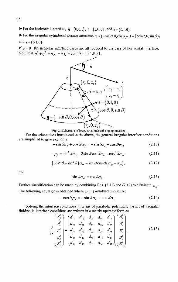
68
• For the horizontal interface, ^ = (0,0,1), t = (l,0,0), and s = (0,l,0).
• For the irregular cylindrical sloping interface, n = (-sin 3,0,cos 3), t = (cos 3,0,sin 3),
and s = (0,1,0) •
If 3 = 0, the irregular interface cases are all reduced to the case of horizontal interface. Note that r]) + rjz = rjztr - r/rtz = cos2 3 + sin2 3 = 1.
V r2 V\ J
s = (0,1,0)
cos 5,0, sin .9)
(r2»°»^5 Fig. 2.1Schematic of irregular cylindrical sloping interface
For the orientations introduced in the above, the general irregular interface conditions are simplified to give explicitly
sin 9u, + cos 3w v /
- sin &u„ + cos i9w.
-pf = sin2 9<rrr -2sin .9cos3an + cos2 3crzz,
(cos2.9-sin2 9jo-rz = sin.9cosi9(crzz -<rrr),
and sin 3a rB = cos 9oa
(2.10)
(2.11)
(2.12)
(2.13)
Further simplification can be made by combining Eqs. (2.11) and (2.12) to eliminate a •
The following equation is obtained where <x is involved implicitly:
- cos 3pr = - sin 3<jrz + cos i9crzz. (2.14)
Solving the interface conditions in terms of parabolic potentials, the set of irregular fluid/solid interface conditions are written in a matrix operator form as
_5_
dr
K
Bi yB[j
<aL
V si *55y
B'r
B'e
KB\J
(2.15)

69
where superscript I stands for irregular interface, and the elements dtj of the above
matrix considering far-field condition are given by
rf''S',7'&
A.,k) , d 82
-riikf rc —5-2/i ' f dz h 8z2
dB= \*lr ' dz
1 ilkr-k,), 3
' r3 89 > dl4=\1r
> d\2 =
8Y HJ
kT ilk, 77 — - e
2
Xk, ilk,-k.\r
. 2 / /
- * / ) ' • , d15=0,
' (2.16)
2ju
(
dz z dz1 r d02\ dz
a 2 ,77z a 2
4 ? 7 r r — 2 7 J S — + dz dz2 r dO2
d21 = L~\kL \
-rfrTi,2kL 1 + — V M.
d 2Xk, d1
fir7?, ~ 5" + dz r 2 2jur d92
2i + 1 + - KKr v M
d„ = r'e^-*L,r^
d2 2 i d3
dz2
|3
33
-\A*T-h)r ! J 2?7r 5 ' „ _ _ ^ _ , ?7X 9;
rd02dz dz3
,3
"^
^24 = L. e l ' t * r "*,,)'•
r2 [ r d6dz z dOdz2 r2 dG
l2d 2 kl d2 kl d2
dz 2rdOl z 2 dz2
In, 2\ 3 3 2 1 54 e4
- ^ ( 2 + ^ ) ^ 3 - + ^ ^ r ^ ^ 2 - + ^ r ^ T 'a zJ r5(92az2 z dz"
d15 = LZ e i ^ - ^ j _2_j.2 s 2 2?7r a3 77277z a4
•n, d0dz r dddz2 r2 d93dz z d&dz3
d A 9
de 35 az
(2.17)
(2.18)
i(kf-kTy ( Afkp 2M
2 2 7 . , 2 \ 3 2 2 a2
1rtJz-+tlr(2-5t},)— + T}rT}i dz ,r ,z r de2
+l\ti-ri)r-^
Ah-tr)r
dn=-
&& + *,£ Mr 7
{2-5rj2)A 2'
+vl 4M
8 ^InAK a2
az //r a#2
r d02dz: + Vzk
2Lr (*-*?)£-* dz2
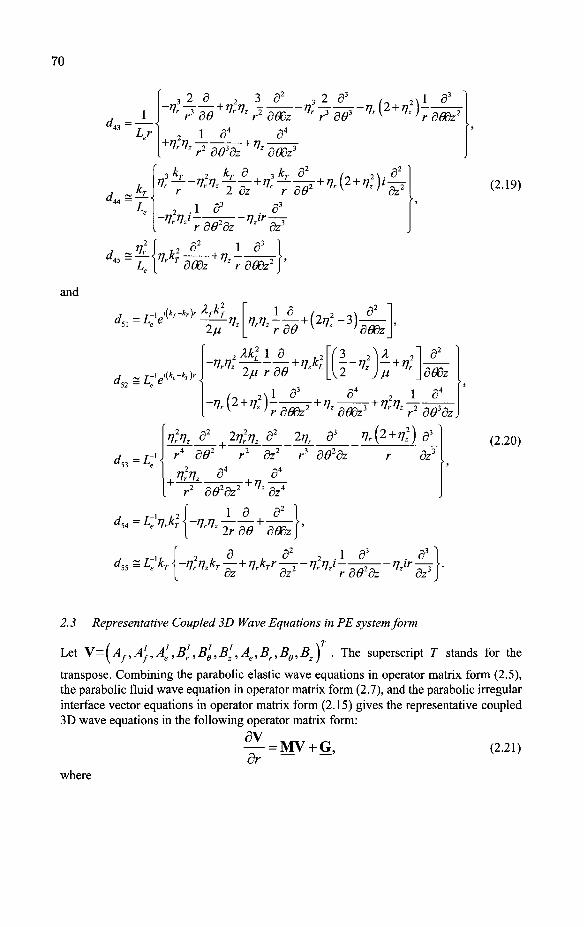
70
Lr
d = ^ 44 ~ L
_ , 2 3
r3 30
3 d2
-K ~ ^ + rlrV, -JTZZ-rf-j-zzr-Vr (2 + 7 , 2 ) -
2 i a4
r 00 dz
r* 80dz
a4
2_j?_ r3803
1 d3
r868zl
r 2 dz
2 .1 e3 . a 3
r z r 8928z h dz'
808z3
2
r dtf rilkir-nlv^Wrk^M^l)i
dz2
d^=^\TJrk2
d0dz +nz
1 d3
r808z2
(2.19)
and
„••(*/-Mr */kf 2ju
^ , - — + (2^-3) a# a6Bz
4 s i : V M | r '
, -4,£,2 1 9 , 2
2/x r 00 2 J/J d06z
1 S4 / . 2\1 d3 d* 2
^ ^ K ^ ^ J ^ ^ r2 8038z
d*=L-:{
ifa d2 Ml, d2 2nr 83 vj^ + ll) 83
B02
Irl: r2 8028z2+T?z*-4
8z2 r3 8028z
dz'
dz3
J ,-i , 2 [ 1 9 d2 1 «« = L, nkT < -Tin, H } ,
1 d3
dS5 s l ; ' * r ^ -?7r277A i r + 7 , V T T - t f r V — r r r
_a_ 5z 3z2 r 5<925z ^ S ?
(2.20)
2.3 Representative Coupled 3D Wave Equations in PE system form
Let \=^Af,AIf,A
,e,B
Ir,B
I0,B
I2,Ae,Br,Bg,Bz
>j . The superscript T stands for the
transpose. Combining the parabolic elastic wave equations in operator matrix form (2.5), the parabolic fluid wave equation in operator matrix form (2.7), and the parabolic irregular interface vector equations in operator matrix form (2.15) gives the representative coupled 3D wave equations in the following operator matrix form:
ev — = M V + G , (2.21) dr
where
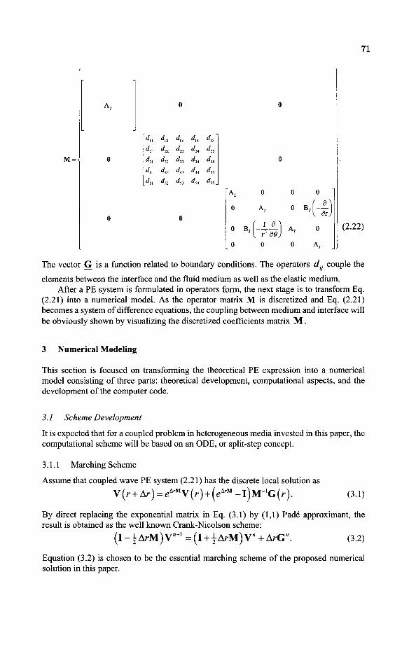
71
M =
du
d21
d„ dtt
« * , .
dn
*n
di2
d«
d52
dn
dn
d„ d„ d„
0
d»
d2i
d„ d«
d»
dn
d2i
d,s
dK d*.
X 0
0
0
B r |
0
<
7~? 0
0
-1 d0)
0
0
A r
0
0
»u 0
A r
(2.22)
The vector G is a function related to boundary conditions. The operators d(, couple the
elements between the interface and the fluid medium as well as the elastic medium. After a PE system is formulated in operators form, the next stage is to transform Eq.
(2.21) into a numerical model. As the operator matrix M is discretized and Eq. (2.21) becomes a system of difference equations, the coupling between medium and interface will be obviously shown by visualizing the discretized coefficients matrix M .
3 Numerical Modeling
This section is focused on transforming the theoretical PE expression into a numerical model consisting of three parts: theoretical development, computational aspects, and the development of the computer code.
3.1 Scheme Development
It is expected that for a coupled problem in heterogeneous media invested in this paper, the computational scheme will be based on an ODE, or split-step concept.
3.1.1 Marching Scheme
Assume that coupled wave PE system (2.21) has the discrete local solution as
V ( r + Ar) = eArMV(r) + ( e A r M - l ) M - ' G ( r ) . (3.1)
By direct replacing the exponential matrix in Eq. (3.1) by (1,1) Pade approximant, the result is obtained as the well known Crank-Nicolson scheme:
(3.2) (l-^ArM)V"+1 =(l + iArM)V+ArG".
Equation (3.2) is chosen to be the essential marching scheme of the proposed numerical solution in this paper.

72
If (2,2) Pade approximant is applied to the exponential matrix in Eq. (3.1), the following higher order scheme is obtained
l-±ArM + —(ArM) 12
I + {ArM +—(ArM) 12
V+ArG". (3.3)
Note that higher, such as (3,3), Pade approximants will make the coefficient of G" not simple as Ar only.
3.1.2 Numerical ODE Formulation for Wave and Interface Equations
To obtain the coefficients matrix of numerical scheme, all the derivatives are expressed in finite difference formulation. The complete derivation and results are very lengthy and therefore referred to the first author's Ph.D. dissertation [16]. Here only parts of them are presented as examples.
For elastic and fluid wave equations, the operators containing derivatives are in a square root. Therefore it is necessary to have an approximation for the square root. The square root approximation can lead to computational phase errors. These phase errors have the physical meaning of limitation in propagation angle [8, 10]. Higher order approximations reduce the phase errors and result in wide-angle models [9]. This issue has been broadly investigated and many wide-angle models were developed in the past two decades. It has been proved that narrow-angle formulation (<23°) is not adequate for sound propagation in shallow water and a wide-angle model must be used instead [7, 8,10]. Nevertheless, most of those models referred to be wide-angle in depth because they are only considering 2-D problems and thus the azimuthal angle is not well discussed until recent years.
Among numbers of square root approximations, a second order approximation [7] is written as
VlTz^l + -Z--Z 2+(9(Z 3 ) . 2 8
For parabolic wave equations, the operator Z is f d 2
7 -^i=f.L,T , 2
1 d 2 A
(3.4)
(3.5)
In the above, f,L,T represent of fluid, longitudinal, and transverse elastic quantities, respectively. If second order is considered in depth where as only first order is considered in azimuth, then the square root approximation is
T\ i a2
dz2 1 5
+ — ee1 = i+ 1 8Z 1 54 1
2k2 dz2 8£,4 dz4 2kfr2 dG2 (3.6)
The above expression is also adopted in Ref. [5]. For consistency and higher accuracy, all the difference formulae are chosen of the second order.
As for U\ + z) in parabolic elastic wave equations for Br and Bg, it can be
approximated via a Taylor series expansion with the polynomial functions
1 + 1 d2 1 8
• +
2 A
dz2 dQ2 ^ 1 -1 d2 3 a4 I
2k2 dz2 8/t4 dz4 2k2r2 dG2 (3.7)

73
With Eqs. (3.6) and (3.7), the parabolic elastic and fluid wave equations can be explicitly discretized. Take fluid wave equation (2.7) as example:
dA •f(iJ)
dr a n
+a fs\
Af(i+2j) + Af(i-2,j)_
Af{iJ+\) + Af(i.j-l).
+ a M Af(Mj)+Af(i-l,j) (3.8)
where ik, ikf
+ afAf(ij)>
ikf * / 2
"•/m '
7T>afi &[kfAz) 2[kfAz) 2{kfAz)
(3.9)
ik,
2{kfrA0)' - , « / • = -
ikf 3ikf ikf
(kfAz) 4(kfAz) (kfrA0)
The subscripts i, j represent the i th grid point in depth, and j th grid point in azimuth. Note that if Ad is chosen so large as 1/A# approaches zero, the equations reduce to two-dimensional case.
In equation for Br, the operator coefficient of Bz is approximated using Eq. (3.7) and
resulting in 1
lH J- \ j 1 ~t" J_ty
d_ ' dz
1 53 3 ds
- + -1 33 \
dz 2k\ dz3 Sk4T dz5 2k2
Tr2 802dz (3.10)
In equation for Bg, the operator coefficient of Br is also approximated using Eq. (3.7)
and resulting in
1 ( 1 d ) _ i ikTyJl + LT I r3dd)~r3kT
1 53 3 - +
1 33 ^
80 2k] 80dz2 8A:r4 808zA 2k\r2 803
(3.11)
As a summary, with the square root approximations and proper discretization, the numerical ODE formulations for elastic and fluid wave equations like Eq. (3.8) and the interface equations can be obtained. The complete results are referred to the first author's Ph.D. dissertation [16] and not shown here. Results for wave equations in Ref. [5] are similar except for its equation of Br where an error occurs in their derivation of wave
equation for Br.
3.2 Computational Aspects
In order to develop the computer code, a number of computational aspects have to be taken into consideration.
For simplicity, taking a horizontal interface problem as an example, Fig. 3.1 schematically shows computation grids and settings. As shown in Fig. 3.1, the upper boundary which usually refers to the ocean surface is assumed to be flat and pressure released
A,\ =0. (3.12)
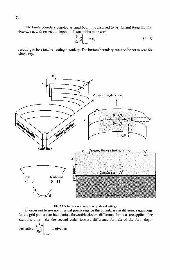
74
The lower boundary denoted as rigid bottom is assumed to be flat and force the first derivatives with respect to depth of all quantities to be zero
h° = 0, (3.13)
resulting to be a total reflecting boundary. The bottom boundary can also be set to zero for simplicity.
T (marching direction)
"SjiilklKety
Port
0 = 0 Starboard
(9 = Q
e
z 1 Initial]
t
r
t
Pressure Release Surface Z = 0
Inii-rt'iici' Z — lit
Pressure Release Bottom Z = 0
V
Fig. 3.1 Schematic of computation grids and settings
In order not to use nonphysical points outside the boundaries in difference equations for the grid points near boundaries, forward/backward difference formulas are applied. For example, at z = Az the second order forward difference formula of the forth depth
derivative, & 4 is given as

75
^-9pl+\6p2~\4p3 + 6p4~p5
(A,)4 (3.14)
where p0 vanishes if pressure release condition is considered. This formula induces
inconsistency error which will be shown in a test case in next section. Nevertheless, the mirror effect, /? . = -p., at pressure release boundaries, /?0 ~ 0, can
be applied so that central difference formula can still be applicable without using nonphysical points as Fig. 3.2 shows. Therefore the second order central difference
d4p formula of the forth depth derivative,
& 4 is given as
P - i ^ + 6Pi -4/>2 + P 3 = ~py + 6 A ~4p2 + p3 = 5/7, -4p2 +p3 ( 3 J 5 )
(Az)4 (Azf (Azf
P-2 >- Nonphysical points
Po=°» P-i=~Pi
> d4p n
atz = Az, —~- = ? dz4
Fig* 3.2 Schematic of pressure release boundary in discrete space. Comparing Eqs. (3.14) and (3.15), it can be noted that considering mirror effect at
pressure release boundaries not only maintains the consistency of using central ditTerence formulas but also reduces the number of grid points from five to three at z = Az.
For the port/starboard sidewall boundaries, they are not pressure released or rigid under most circumstances except for numerical tests. In realistic situations, they are not known and have to be computed and provided as boundary conditions of Dirichlet type
QL,a=fo,a- (3-16)
2D (r-z) solutions may be the most straightforward answers provided for sidewall
boundaries. A computer code is developed to implement the marching implicit scheme (3.2).
However, it must be mentioned that the mathematic and numerical development of the proposed model does not contain the density variation and other capability enhancement, the computer code is basically a research code. It still needs some efforts to turn this code into a practically working code like other well known models, say, FOR3D.
The geometry of propagation has been presented in Fig. 3.1. The data structure should be particularly noticed since this model deals with a heterogeneous problem. That is, at a

76
single grid point, there are more than one unknown quantities. Each field quantities Af,Ae,Br,Be,Bz is stored in separate matrices at the beginning and in its final form.
However, during the calculation stage, solving the unknowns requires these field quantities to be organized as a single vector at each range step. The coefficient matrix corresponding to this unknown vector is thus constructed as the following figure shows along with the structure of the unknown vector. The figure shows an example of 9 azimuth sections (side-wall boundaries excluded). Blue dots represent nonzero elements which are the coefficients of the difference equations. It can be seen that the matrix is formed as a band-matrix. Dark lines indicate different azimuth sections whereas the red dashed lines showing the five interface equations between the fluid and the elastic wave equations which are colored with light blue and olive boxes, respectively. The unknown vector is a column shown at right hand side of the coefficient matrix.
Fig. 3.3 Data structure of the coefficient matrix and unknown vector.
4 Model Appraisal
In this section, several test cases are investigated to validate the model and also to show the model's application and ability. Exact solutions to the coupled 3D wave propagation problems are practically unachievable due to complexities in environment and boundaries. To validate models claiming to solve these problems is therefore limited.
In the following, several examples will be presented to start from the simplest two-dimensional range-independent problem for waves in fluid only, and finally to the coupled 3D wave propagation model with irregular interface.

77
4.1 2D Fluid Waves in Range-Independent Environment
Being the first step to validate the model, this example is focused on testing the numerical marching scheme Eq. (3.2). Also the effect of considering the mirror effect on pressure release boundaries as prescribed in previous section is presented.
Considering a two-dimensional ( r z ) plane, the upper and lower boundaries are both
flat and pressure-released, and the medium in between the two boundaries is pure fluid only without any energy absorption. The environment is totally range-independent.
Numerical ODE formulation for the 2D fluid wave equation can be obtained by applying the square root approximation (3.4) and (3.5) resulting similar to Eq. (3.6) as
dAf
~dr~ -ik, _Li_.
2k) dz2
aO Sk) dz4 V
(4.1)
To find the general solution to the above equation, one can use the method of separation of
variables given the initial condition A (o z) = sin — I a nd obtain
= exp < -ir (TVIH)1 (7tlH)A
2kf Sk} •sin — . (4.2)
Using the presented numerical model, a banded matrix is formed to solve the problem with computation parameters set as Az = 0.1/L,Ar = 3/L, where sound speed c is 1500
m/s, sound frequency / is 200 Hz, water depth H is 60 m, wavelength ; is 7.5 m. Figure
4.1 compares the absolute value of computed solutions using (l,l)/(2,2) Pade scheme and sided/central difference near boundaries for range 0 -12 km. It can be clearly seen that errors accumulate from the upper and lower boundaries if mirror effect is not considered and sided difference is applied. Also higher order scheme, such as (2,2) Pade scheme, is more sensitive to such errors from boundaries. However, if mirror effect is taken into account, then the errors are removed and (2,2) Pade scheme produces better results as it is expected.
error norm = 9 5 4 9 2 e - 1 error norm = 3 .3786e-3
-r —
- 0.4 -
n n
: PA -.
u.a
„
0 4 -
(1,1) P a d e + s ided di f ference near boundar ies
error no rm - 6 .3677e+O20
(1,1) P a d e -*• central d i f ference wi th mirror effect near boundar ies
error norm = 1.7978e-3
0"4
no -
-1--1-H _ ,
— : - *aL
\ -
(2,2) P a d e + s ided di f ference near boundar ies (2.2) P a d e + central d i f ference wi th mir ror effect near boundar ies
Fig. 4.1 Comparison between the computed solutions using (l,l)/(2,2) Pade" scheme and sided/central difference near boundaries.

78
By this test case, the marching scheme using (l,l)/(2,2) Pade approximations are validated. The improvement of considering mirror effect near pressure release boundaries is also presented. This suggests the consideration of mirror effect in all computations when pressure release boundaries occur.
4.2 2D Elastic Waves in Range-Independent Environment
The elastic wave governing equations are coupled for 3D propagation as two individual systems, {Ae} and {Br,Be,Bz}. For 2D propagation, #-derivatives are dropped so that
Br is uncoupled from the equation of B$, therefore the governing equations are further
uncoupled into three independent sets, lAe}, {Be\, and iBr,Bz\. Provided there is no
coupling mechanism on boundaries, 2D elastic waves problem can be resolved by separately finding the solutions of the three systems.
Given the same flat and pressure-released upper and lower boundaries as in the previous case for fluid wave problem, since equations of iA\ and {Be} are of the same
form as that of \Af], similar analytic solutions and results presented in the previous case
can be obtained. Hence here we will focus on the two-variable coupled system, {Br,Bz\ •
Note that under these pressure-released boundary conditions, if Bz is initially unexcited,
i.e., B\ = 0, then B will be decoupled from the equation of B • Therefore the problem
is reduced to the same form of \Af] , and the whole Bz field will be completely silent,
thus the equation of Bz turns out to be trivial and its calculation may be saved.
After applying square root approximations (3.6) and (3.7), the two-variable coupled system, iBr,Bz\ writes
^ = ikT dr T
dr
( 1 82 1 d4^
2k2 dz2 Sk4 dz*
JLJ?L__L_3l y2k2 dz2 %k* dz4
i f Pi 1 Pi3 -X F)5 ^
B_. ( 1 =)2 1 a 4 "\ • f rs 1 a3 o a 5 A
(4.3)
^i d3 3 55
- + -dz 2k* dzs Sk4 dz5
As before, the analytic solution to Eq. (4.3) is desired. The strategy to solve Eq. (4.3) is
summarized as two steps. The first step is to solve the parabolic equation for Bz, and this is
followed by solving the parabolic equation for Br with the part containing derivatives of
B known as the inhomogeneous source term.
By the method of separation of variables, Bz can be derived in the form of
Bz=e\p(-ikTg2r)lciexp(£lz)+C2exp(-llz) + Cisin(£2z) + C4cos(£2zjj, (4.4)
where the functions with underline are the eigenfunctions, and £l,£2 are related to the
eigenvalues as

79
••yfikrjj: l + 2 ?2 + l . (4.5)
Note that the given boundary conditions Bz (r,0)=Bz (r,H) = 0 are not sufficient to define
the coefficients C ; . However, with proper initial conditions input, the coefficients can be
determined. It is obvious that s j n | r^Lz ] for any integer n can satisfy the zero boundary
U J conditions. Further more, it is of the same form with one of the eigenfunctions, sin(^2z) •
Therefore, if the initial filed is given as Q s m TLZ I, where C0 is a constant, then ° \H )
Bz(0,z) = C1exp(V) + C2exp(-Az) + C3sin(V) + C4cos(^2z) = C0sin(— Z\ ^ ^
the coefficients in Eq. (4.4) can be determined as C, = C2 = C4 = 0, and C3 = C0 a known
constant. Also it leads to nn
H , so that the eigenvalues are given as
Sn nn
ykTH j
r \ nn
\kTH j
and thus the analytic solutions to B is then written as
Bz = C0expl-ikT nn
ykTH j
1 + —
f A4
nn l K,rp±l J I . fnn
sin — z
(4.7)
(4.8)
The analytic solution to A, in the previous case can be verified by the above equation as
well where « = 1,C0=1-
Next step is to substitute Eq. (4.8) into Eq. (4.3) to solve the equation for Br. After the
substitution, it reduces to
55, dr K2k2
Tdz2 %kATdz" j
B,
+C0iexp(-ikTg2nr)
nn 1 - + — kTH 2
V nn
\kTH j
V nn
\kTH j
(4.9)
cos frm_ ^
\H j
Equation (4.9) is an inhomogeneous PDE which can be solved by eigenfunction expansion method [13]. If n = 2,C0=l is chosen to have the initial condition for B being
Bz (r, 0) = sin[ — z 1» and a static initial condition for Br, i.e., Br (r, 0) = 0, the solution
to Eq. (4.9) is obtained as
Br= Z 4 / i 4 o ( e " v - e " v )
— r ^ — r z ^-sin ' nn ^
n=w,..fr(n2-4)(AH-A2) H (4.10)

80
where
4>=» 71
yKjH j + 4
f \ n
\ K-pi~t j
+ 12 r V
71
f \ nn
\ K-T-JLI. I
nn
yKj-H j
ykTH j
,n = l ,3 ,5,--- .
y /\r\ ZAlXj
f \ 71
ykTH j
2 { y 71
\ Kjii i (4.11)
18m
mmmmmmm
0« U\\ ' H * M
- s !,I i Range (KM)
ItlllttHIHiMU •
tllllllllMlKltM IIIIIMIItlliltMl
0 5 10 15 20
Range (KM) Fig. 4.2 Absolute value, real part, and imaginary part of the numerical solutions to 2D elastic wave problem (4.3).
Comparison of computed and analytic solutions of B
-(1,1) Pade (2,2) Pade
-Analytic Solution
Range (km)
Fig. 4.3 Comparison of (1,1 )/(2,2) Pade schemes and analytic solutions of B at depth of 18 m.

81
Given the depth H = 99 m, wave frequency / = 100 Hz, transverse wave speed
cT = 900 rn/s, the numerical solutions of Bz and Br are plotted in Fig. 4.2 for range 0 -
20 km considering the absorption coefficient being 0.5 dB per wavelength. Setting the
computational parameters Az = 0.2/1,. and Ar = 8 ^ , the numerical results of Br agree
well with the analytic solution at selected depth of 18 m shown in Fig. 4.3. However, (1,1) Pade scheme does not provide as good prediction as (2,2) Pade scheme for this case.
4.3 Coupled 2D Waves with Irregular Interface
In this test case, at first a down-slope wedge is considered then an up-slope wedge. Both slope ratios are 1:20, or about +2.86°, and the water depth at source location is 200 m. A Greene's source is placed at depth of 30 m, the computation parameters are set as Az = 0.18m, Ar = 3.6ra , and the absorption coefficient being 0.5 dB per wavelength.
Figure 4.4 shows the computed solutions in water column, \A,1, in the upper two plots.
Up-slope
j y . l A ^ d z / H ,
...
' . "*" '•^^^
- ™ - ~ Down-sfope. C T = 40 m/s (A.: p. ~ 1800 ; 1}
Down-stope. C T = 900 m/s (A.: n ~ 3 : 2)
Up-slope, C T = 900 m/s (X : p. ~ 3 : 2)
i ~ - -E3~ : __ i ^^^
— Shear £ffect^*%vj'-^
!HP yU
~" "0 0 5 1 1.5 2 2.5 3 3 5
Range (km) Fig. 4.4 Comparison between the calculated results of up/down-slope wedge with low/high shear wave speed.
The lower plot compares the depth averaged energy along the propagation range for four difference situations. The green solid line represents the result calculated in down-slope wedge with very low shear wave speed (CT = 40 m/s) comparing to the red dashed line where the shear wave speed is 900 m/s. These two line does not differ too much, i.e., shear effect is not obvious in down-slope wedge. In up-slope wedge, energy in water column is expected apparently decreasing due to more interaction between wave and bottom as shown in the figure. The blue dotted line represents the result calculated in

82
up-slope wedge with shear wave speed being 40 m/s whereas the black solid line is the case with cT = 900 m/s. It can be seen from the figure that there is noticeable difference due to
shear effect for up-slope wedge. More energy of water column is transferred into bottom as shear wave.
4.4 Coupled 3D Waves with Irregular Interface
It has to be noticed as mentioned before that the analytic solutions to such problems are inaccessible.
For simplicity, the upper and lower boundary conditions are pressure released boundaries, and the two side-wall boundary conditions are zeros as well. Given the environment setting being the same as before except for total depth of H = 70 m and a range-dependent bathymetry H,(r)- For sound frequency of 25 Hz, the initial field is
placed at r0= 1082.3 ni to satisfy far-field approximation ft.r>100, i = f,L,T • The
computational parameters are set as: Ar = OAAj = 14.4 m, A8 = 0.5° , and
Az = 0.015/^ =0.54 m. It must be noted that Az is chosen so small to have accurate
solutions because of the interface effect. Starting from r0, the initial field is propagated 150
m which is about 10 range steps, and the computation span is 20 degrees which consists 21 sections including two side-wall boundaries. The bathymetry is defined as // ;(r0) = 35,//,(r0+50)=36,// ;(r0+100) = 34, and H, (r0 +150) = 37, as shown in Fig.
4.5. It must be emphasized that the bathymetry is given of axial symmetry to be consistent with the irregular interface defined and shown in Fig. 2.1.
Ar = 0.4A,. = 14.4m A6> = 0.5°
Az = 0.015^ =0.54m
-34.
— -35.
1 . -36,
-37
-300 K
20"
__—-"~T 1240 - - H 1220 1200
Range (X-axis, m;
Range (Y-axis, m)
Fig. 4.5 Schematic of 3D bathymetry and other computational settings.
To have a 3D initial field instead of an Nx2D field, all the field is initially static except for Af(r0,d = 0,z) is excited by a normalized sine function. The calculated results are
plotted in Figs. 4.6 - 4.7 where the absolute values of Af,Ae,Br,Be,Bz are shown. The
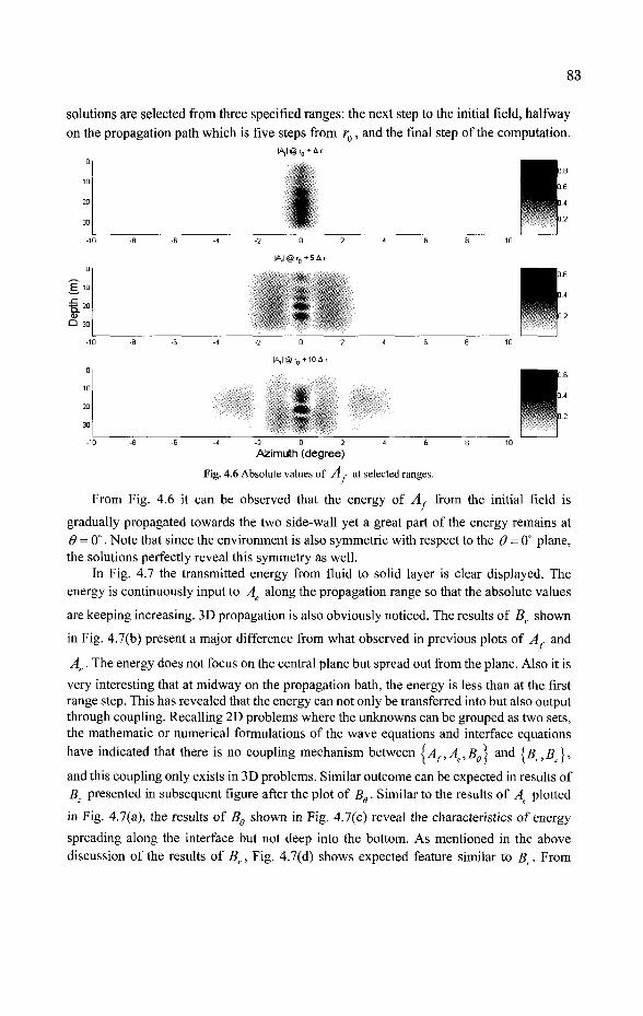
83
solutions are selected from three specified ranges: the next step to the initial field, halfway on the propagation path which is five steps from r0, and the final step of the computation.
IA,l©r0+Ar
£ 10
Q 30
0 2
I A , l @ r 0 + 5 A ,
-2 0 2
IA,l@r0 + 10Ar
Azimuth (degree) Fig. 4.6 Absolute values of A r at selected ranges.
From Fig. 4.6 it can be observed that the energy of Af from the initial field is
gradually propagated towards the two side-wall yet a great part of the energy remains at 9 = 0°. Note that since the environment is also symmetric with respect to the 0 = 0° plane, the solutions perfectly reveal this symmetry as well.
In Fig. 4.7 the transmitted energy from fluid to solid layer is clear displayed. The energy is continuously input to Ae along the propagation range so that the absolute values
are keeping increasing. 3D propagation is also obviously noticed. The results of Br shown
in Fig. 4.7(b) present a major difference from what observed in previous plots of A, and
Ae. The energy does not focus on the central plane but spread out from the plane. Also it is
very interesting that at midway on the propagation bath, the energy is less than at the first range step. This has revealed that the energy can not only be transferred into but also output through coupling. Recalling 2D problems where the unknowns can be grouped as two sets, the mathematic or numerical formulations of the wave equations and interface equations have indicated that there is no coupling mechanism between lAf,Ae,Be) and [Br,B\,
and this coupling only exists in 3D problems. Similar outcome can be expected in results of Bz presented in subsequent figure after the plot of Be • Similar to the results of Ae plotted
in Fig. 4.7(a), the results of Be shown in Fig. 4.7(c) reveal the characteristics of energy spreading along the interface but not deep into the bottom. As mentioned in the above discussion of the results of Br, Fig. 4.7(d) shows expected feature similar to B • From

84
interface equations or numerical formulation, this feature shared by B and B is due to
azimuth coupling at interface and thus is a kind of 3D effect.
•
•5 .—-r—r~
m
*» t ~4
:"
mf
mm
(a) (b)
HI
', . . 1 M l
llliflll
B* AzfmuHiEdtgnM) AzmttKtfegnw)
(c) (d)
Fig. 4.7 Absolute values of (a) Ae (b) Br (c) 5 t f (d) # , at selected ranges.
The 3D example tested in this section is highly restrained and simplified to focus on the primary concerns, i.e., realization of the proposed model and how it works with coupled fluid/solid medium with irregular interface. It has to be emphasized that a major difference between considering fluid bottom and real elastic bottom is the demand in computation resources especially the CPU time. This is due to the increasing of the number of physical quantities in elastic bottom, from single one to four. The additional three, Br,Be,Bz,
account for shear waves. Under the condition of same grid points, the coefficient matrix considering shear waves is 4 x 4 times larger than fluid bottom. In other words, the range of interested problem is therefore practically limited. Nevertheless, this kind of technical shortness can be expected to be resolved just like decades ago, and the emphasis must be placed on pursuing the completeness in describing the problem and its solution.
5 Summary
This paper has introduced a modified mathematical model to 3D coupled fluid/solid wave propagation problem and also developed its computational model and a research code. The numerical results produced by this computer code has presented good agreements with analytic solutions which reveals that this computer code produces satisfactory results. The

85
validation has also shown that the stable marching scheme which implements implicit finite difference method is accurate.
The emphasis has been placed on the development of the numerical model which can solve 3D fluid, elastic, or fluid/solid coupled wave propagation problems. The underlying idea is applying parabolic displacement potential functions to rewrite the wave equations and interface equations, and then using implicit finite difference method to solve the ODE system. Pade series expansion has been used to improve the accuracy in range direction. Since the proposed numerical model and computer code are new, analytical validation of the scheme has been conducted for several problems. The proposed model has been successfully applied to simulate the fluid/solid coupled wave problem.
From both mathematical and numerical modeling, two major differences can be found in 2D/3D comparison, with/without shear effect. A 2D problem is a simplified special case from 3D problems where all the five unknowns [Af,Ae,Br,Bg,Bz\ representing the
parabolic functions of displacement potentials are coupled together and must be solved simultaneously. The simplest case is 2D problem without shear effect and its unknowns are \Af, Ae) only, that means the energy will be shared by the two quantities only. This is also
true for 3D problem without shear effect. If shear effect is to be considered in a 2D problem with only Af excited by a waterborne source, then the unknowns become lAf,Ae,Bg)
which means the energy will now be shared by one more quantity, Bg. Note that if
{Br,B\ is not initially static, then this set of unknowns should also be solved yet as an
independent problem so that the solution of j A f,Ae, Be ] will not be affected. For the most
general case, a 3D problem sustaining shear effect includes all the unknowns iAf,Ae,Br,Bg,B2] , and the energy will shared by these five quantities. In other words,
the energy of compressional waves {A, and Ae) can be overestimated if shear effect is
ignored whether in 2D or 3D problems. Also the energy can be overestimated even when shear effect is considered in 2D case, because the energy coupling mechanism between {A,, A ,Bg) and iBr,B\ is missed. Table 5.1 compares 2D/3D cases with/without shear
effect.
Shear Effect
X
X
1 ahle 5
2D/3D
2D/3D
2D
3D
1 ('ninpiirjinn nl 21) .»l) CUM'.- with uilhuiil .••hear effect. . . . _ Compressional Wave Unknown Quantities _,. r _ . Energy Overestimated
K'4} @ {Af,Ae,Bg} and {Br,Bz} O
{Af,Ae,Br,Bg,Bz)
3D effects are found to occur from four sources. First, the initial field can decisively affect the propagation pattern including how the waves spread in azimuth direction. Second, the #-coupling terms (derivatives with respect to azimuth) in the governing equations and interface conditions reflect the constitutional properties of 3D wave propagation. Third, the environment, including the geometry and the acoustic parameters of the medium, has direct influence on the wave propagation path by reflection, refraction, and scattering. Hence a

86
3D environment will definitely induce 3D effects. Finally, 3D distributed boundaries will induce 3D effects as well.
Although the irregular fluid/solid interface investigated in this dissertation is range-dependent, £?-variation is not considered in the formulation. As Fig. 2.1 shows, the
second unit tangent vector s(sr,sg,sz} is set to (0,1,0) so that a cylindrical irregular
interface is obtained. In other words, this interface is of axial symmetry and this is why it is drawn as a frustum of right circular cone in Fig. 2.1. This assumption is a serious drawback of the model since such interface will only reflect waves in fixed 8 planes, i.e., geometric #-coupling at interface is ignored. To deal with a real 3D problem, the interface has to be generalized to include variation of bathymetry in 0 direction. For example, if the interface as shown in Fig. 2.1 is counterclockwise rotated an angle q> respective to unit direction vector t , then three unit direction vectors are given by
r\] f-sin>9cos#>, -sin <p, cosi9cos#>
t - = | cos.9, 0, sin,9 I. (4-12)
sj [ sini9sin<z>, cos<p, cos>9sin#>
Although a modified mathematical formulation and a novel numerical model for 3D fluid/solid coupled wave propagation problem considering irregular interface this dissertation has been developed and coded as a research prototype program C4PM, it is only a beginning for this challenging topic. There are several issues regarding mathematical and numerical enhancements to the modeling and theoretical completeness, namely, wide angle expansion in azimuth, proof of the energy-conserving property such as the proof for LSS wave equation given in Ref. [15]. Each of these issues can be a great improvement and validity proof of the proposed model.
Acknowledgement
This work is supported by National Science Council of Republic of China. The authors would like to thank Dr. Yu-Chiung Teng for her encouragement and discussion.
References
1. Lee, D., Nagem, R. J., Teng, Y.-C, and Li, G. (1996) "A Numerical Solution of Parabolic Elastic Wave Equations," in Proc. 2nd Int'l Conf. Theo. And Comp. Acoust., eds. D. Lee, Y.-H. Pao, M. H. Schultz, and Y.-C. Teng, World Scientific Pub. Co., Singapore.
2. Shang, Er-Chang and Lee, Ding. (1989) "A Numerical Treatment of the Fluid/Elastic Interface Under range-dependent Environments," J. Acoust. Soc. Am., Vol. 85, No. 2, pp. 654 - 660.
3. Lee, D„ Nagem, R. J., Resasco, D. C, and Chen, C.-F. (1998) "A Coupled 3D Fluid/solid Wave Propagation Model: Mathematical Formulation and Analysis," Applicable Analysis, Vol. 68, pp. 147 - 178.
4. Sheu, T. W.-H., Chen, S.-C, Chen, C.-F., Chiang, T.-P., and Lee, D. (1999) "A Space Marching Scheme for Underwater Wave Propagation in Fluid/solid Media," J. Comput. Acoust., Vol. 7, No. 3, pp. 185 - 206.
87
5. Lee, D., Nagem, R. J., and Resasco, D. C. (1997) "Numerical Computation of Elastic Wave equations," J. Comput. Acoust., Vol. 5, No. 2, pp. 157 - 176.
6. Nagem, R. J. and Lee, D. (2002) "Coupled 3D Wave Equations with Fluid/solid Interface: Theoretical Development," J. Comput. Acoust., Vol. 10, No. 4, pp. 431 -444.
7. Lee, D. and Schultz, M. H. (1995) NUMERICAL OCEAN ACOUSTIC PROPAGATION IN THREE DIMENSIONS, World Scientific, Singapore.
8. Jensen, Finn B., William A. Kuperman, Michael B. Porter, and Henrik Schmidt, (2000) Computational ocean acoustics, Springer-Verlag, New York.
9. Lee, Ding, Pierce, Allan D., and Shang, Er-Chang (2000) Parabolic equation development in the twentieth century, J. Comput. Acoust., Vol. 8, No. 4, pp. 527 -637.
10. Lee, Ding, and McDaniel, S. T. (1987) Ocean acoustic propagation by finite difference methods, Comp. Maths Applic, Vol. 45, No. 5, special hardcover issue, published by Pergamon, New York (1988).
11. McDaniel, S. T. and Lee, Ding (1982) A finite-difference treatment of interface conditions for the parabolic wave equation: The horizontal interface, J. Acoust. Soc. Am., Vol. 71, No. 4, pp. 855 - 858.
12. Nagem, R. J., Lee, Ding, and Chen, T. (1995) Modeling elastic wave propagation in the ocean bottom, J. Math. Modeling and Scientific Computing, Vol. 2, No. 4, pp. 1-10.
13. Farlow, Stanley J. (1982) Partial Differential Equations for Scientists and Engineers, John Wiley & Sons, Inc., Singapore.
14. Lee, Ding (1974) "Nonlinear multistep methods for solving initial value problems in ordinary differential equations," Ph.D. paper, Polytechnic University of New York.
15. Chen, C.-F., Lee, D., Hsieh, L.-W., and Wang, C.-W. (2005) "A discussion on the energy-conserving property of a three-dimensional wave equation," J. Comput. Acoust., to appear in Vol. 13, No. 4.
16. Hsieh, Li-Wen (2005) "Modeling 3D Wave Propagation in the Ocean Coupled with Elastic Bottom and Irregular Interface," Ph.D. dissertation, National Taiwan University, Taiwan, R.O.C.


Journal of Computat ional Acoustics © IMACS
REFLECTIONS F R O M STEEL PLATES W I T H DOUBLY P E R I O D I C A N E C H O I C COATINGS
SVEN IVANSSON
Swedish Defence Research Agency, SE-164-90 Stockholm, Sweden
A thin rubber coating with cavities in a doubly periodic lattice can redistr ibute sound energy, normally incident on a steel plate, in the lateral direction. At high frequencies, propagating reflected beams appear in a discrete set of nonnormal directions in the surrounding water. The phenomenon is illustrated by pulse measurements in a water tank. The results are modeled by adapt ing modern computat ion techniques for electron scattering and band gaps in connection with photonic and phononic crystals. At lower frequencies, with only one propagating reflected beam in the water, differential evolution and winding-number integral algorithms are applied to design coatings with low reflectance. A stochastic resampling algorithm is adapted for accurate characterization of the par ts of parameter space with favorable properties.
Keywords: invariant embedding; multiple scattering; tank measurements; nonlinear optimization.
1. Introduction and Summary
Already during the second world war, rubber coatings with air-filled cavities were used on submarines, for anechoic purposes.1 Such coatings are said to be of Alberich type. When sound from an active sonar enters the coating, Fig. 1, energy that is scattered by the cavities can be absorbed by the rubber material, and the reflection amplitude can be reduced significantly. The mechanism of the echo reduction has been discussed by Gaunaurd et al., based on resonance theory, but multiple scattering among the cavities was not included in a rigorous way.2 More recent homogenization approaches,3 '4 are also deficient in this respect.
In the present paper, reflections of normally incident plane waves by steel plates with Alberich coatings are modeled numerically with a semi-analytical method briefly reviewed in Sec. 2. It has been borrowed from atomic physics5 and applied in recent years to studies of band gaps for photonic and phononic crystals.6,7 Sound propagation through a sequence of layers, with or without cavities, is handled recursively by the invariant embedding or Riccati method.8 The wave field scattered by each cavity is expanded in spherical wave functions, and multiple scattering among the cavities is incorporated in a rigorous self-consistent way. Transformation formulas between spherical and plane waves provide the coupling to the plane waves needed for the recursive invariant embedding treatment of multi-layered cases. A basic computational example is given in Sec. 3. It is for the fundamental case with spherical cavities, but other cavity shapes can be handled as well.
89

90
normally incident plane-wave sound energy
t water t T T
O coating Q Q
steel plate
water y
Fig. 1. Left: A steel plate in water is covered with an Alberich rubber coating with spherical cavities. Right: The cavity lattice with period d is viewed from another perspective. Lateral xy coordinates are introduced.
At high frequencies, the theory predicts propagating nonnormal beam or plane-wave arrivals, after the initial specularly reflected arrival. The phenomenon is related to the Praunhofer diffraction patterns for a multiple-slit aperture in optics. Pulse measurements together with modeling results are presented in Sec. 4, where these later arrivals show up.
The computational technique in Sec. 2 is fast compared to purely numerical methods like the finite element method.9 Numerical coating design with many objective function evaluations becomes feasible. Two different techniques are applied in Sec. 5: a differential evolution (DE) algorithm to achieve low reflectance within a wide frequency band, and a winding-number integral technique to obtain vanishing reflectance at a specified frequency. The identification of the parts of the parameter space resulting in favorable anechoic properties is aided by a stochastic resampling algorithm borrowed from inverse theory.10 Reflection elimination is illustrated with a coating not much thicker than 5 % of the wavelength, and an apparent splitting of a reflected pulse is explained.
2. Computational Method
2.1. Invariant embedding
A right-hand Cartesian xyz coordinate system is introduced, with xy in the interface plane between two homogeneous solid or fluid half-spaces. Sound waves with time dependence exp(—\wi) are considered, where u is the angular frequency. In the solid case, because of three possible polarizations, P,SV,SH, an incident plane wave in the positive z direction gives rise to three reflected and three transmitted waves.8 Including the three incident-wave polarizations, a 3x3 reflection-coefficient matrix TZB and a 3x3 transmission-coefficient matrix TB may be formed. These matrices depend on the lateral wavenumber, which is, however, constant among all seven waves according to Snell's law. For an incident plane wave in the negative z direction, the matrices TZA and TA are introduced analogously.
An "interface" at z = 0 is considered next, with a two-dimensional periodic array of cavities. The centers of the scatterers, right panel in Fig. 1, have xy coordinates given by
R = (a;, y, 0) = m • {d, 0, 0) + n • (0, d, 0) , m,neZ , (1)
where d is the lattice period. R / T (reflection/transmission) matrices TZB-TB and 1ZA,T~A can still be defined. However, reflected and transmitted waves appear with lateral wavenumber

91
vectors different from that of the incident wave, ley. By a Fourier expansion in x,y, the appearing lateral wavenumber vectors are k|| + g, where g belongs to the reciprocal lattice
g = (kx,ky,0) = m • (27r/d, 0,0) + n • (0,2n/d,0) , m,n£Z . (2)
Displacement coefficients are used for the R / T matrices. With r = (x, y, z), the displacement vector for an incident, reflected or transmitted plane wave is a multiple of
u ( r ) = e x p ( i . K ^ - r ) - e , . (3)
The time dependence exp(—itot) is suppressed, and j = 1,2,3 for a wave of type P,SV,SH, respectively. Furthermore, s = +(—) for a wave in the positive (negative) z direction, and
K±. = k , | + g ± [ ^ 2 / c ? - | k | | + g | 2 ] 1 / 2 - ( 0 , 0 , 1 ) = -(s in0cos0,s in0sin<£,cos0) (4)
where Cj is the compressional-wave velocity a when j = 1 and the shear-wave velocity (5 when j = 2,3. The angular variables 8, 4> of K * are defined by (4), with a possibly complex cosfl. The vectors e , = e j (Kr\ ) , finally, are defined as usual by ei = (sin 0 cos 0, sin 0 sin 0, cos#), e2 = (cos 0 cos >̂, cos#sin^>, — sin#), e3 = (— shi(/>, cos</>, 0).
Including one scatterer interface within the rubber layer, four interfaces are involved in the left panel of Fig. 1. Individual R /T matrices can be combined recursively. With R / T matrices 1ZBI,1~BI, 1ZAI,T~AI and 1ZB-2,1~B2, T^-A2,TA2 for two interfaces given in the order
of increasing z, and phase shifts included to account for layer thicknesses, the following formulas are easily established for the total R / T matrices 1ZB,T~B:5'S
TIB = 1IBI + TAi • 1ZB2 • [I - TlA\ • ̂ s 2 ] " 1 • TB1 (5)
TB = TB2 • [I - KAI • KBI}-1 • TB\ , (6)
where each I denotes the appropriate identity matrix. Formulas for TZA,TA are analogous.
2.2. Interface with periodically distributed scatterers
Explicit expressions for the R / T matrices in Sec. 2.1 are well known for an interface between two homogeneous half-spaces.8 To handle an interface with periodically distributed scatterers, the following spherical vector solutions to the wave equations can be used:7
ufm(r) = ^.V(/ i(W«Wn(e,0)) (7)
,M,,_.,,,,, ,m i ( i air(M) „_,_, wry, O) = i/,(^) • 7 W W ) • ( ^ - ^ • e 2 ( 0 - - ^ • e 3 ( r ) ) (8)
< ( r ) = ^ • V x < ( r ) (9) CO
where r = |r| and 6,<p are the angular variables of r. Yjm = yjm(6', (/>) are the surface spherical harmonics. The index £=0,1,2,.. with m=-l,..,l, but it is understood that UQQ = u ^ = 0. The notation u°^ ,u°^ f ,u^ an(^ uhn'uhrf >uhn 1S usec^ f° r t n e t w o basic cases with ft as the spherical Bessel function jj and fi as the spherical Hankel function h;
+, respectively.
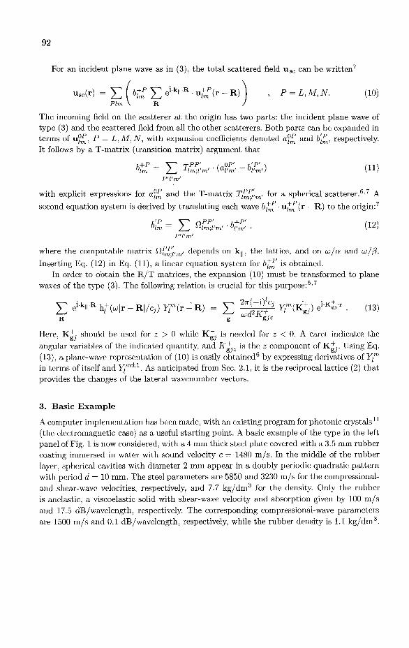
92
For an incident plane wave as in (3), the total scattered field u s c can be written
, P = L,M,N. (10) uSc(r) = £ ( H? £ e l k " R • O - R) ) Plm V R /
The incoming field on the scatterer at the origin has two parts: the incident plane wave of type (3) and the scattered field from all the other scatterers. Both parts can be expanded in terms of u ^ , P = L,M,N, with expansion coefficients denoted a ^ and b^, respectively. It follows by a T-matrix (transition matrix) argument that
hm = Z.^ Tlm;l'm' ' (al'm' + h'm') ( H ) P'l'm'
with explicit expressions for a ^ and the T-matrix T^Vm, for a spherical scatterer.6,7 A
second equation system is derived by translating each wave bf • u t , (r — R) to the origin:7
E^w^:, (12) ,'p _ sr^ c,pp' °lm
where the computable matrix fi^(/m/ depends on ku, the lattice, and on to/a and to/(3.
Inserting Eq. (12) in Eq. (11), a linear equation system for bfm is obtained. In order to obtain the R / T matrices, the expansion (10) must be transformed to plane
waves of the type (3). The following relation is crucial for this purpose:5 '7
£ e i k " ' R h + M r - R | / C j ) Y,m(r - R) = £ 2~^=^ > T ( K ± ) e ^ V . (13) R g %j*
Here, Kl"- should be used for z > 0 while K~- is needed for z < 0. A caret indicates the angular variables of the indicated quantity, and K^- is the z component of Kl_-. Using Eq. (13), a plane-wave representation of (10) is easily obtained6 by expressing derivatives of Y";m
in terms of itself and y ;m ± 1 . As anticipated from Sec. 2.1, it is the reciprocal lattice (2) that
provides the changes of the lateral wavenumber vectors.
3. Basic Example
A computer implementation has been made, with an existing program for photonic crystals11
(the electromagnetic case) as a useful starting point. A basic example of the type in the left panel of Fig. 1 is now considered, with a 4 mm thick steel plate covered with a 3.5 mm rubber coating immersed in water with sound velocity c = 1480 m/s. In the middle of the rubber layer, spherical cavities with diameter 2 mm appear in a doubly periodic quadratic pattern with period d = 10 mm. The steel parameters are 5850 and 3230 m/s for the compressional-and shear-wave velocities, respectively, and 7.7 kg/dm 3 for the density. Only the rubber is anelastic, a viscoelastic solid with shear-wave velocity and absorption given by 100 m/s and 17.5 dB/wavelength, respectively. The corresponding compressional-wave parameters are 1500 m/s and 0.1 dB/wavelength, respectively, while the rubber density is 1.1 kg/dm3 .

93
Curve (c) in Fig. 2 shows the frequency dependence of the corresponding reflectance. As compared to curves (a) and (b) for an uncoated and a homogeneously coated reference case, respectively, significantly reduced reflectance appears in the 10-60 kHz interval. At very low frequencies, the plate is thin compared to the wavelength and the reflectance drops.
According to (2)-(4), with k|| = 0, only the normal beam is propagating in the water below c/d = 148 kHz. Nonnormal beam quartets become propagating at 148 kHz for (m,n) = (±1,0) and (0,±1) in (2), and at c^/2/d = 209.3 kHz for (m,n) = (±1,±1) . The corresponding small contributions to curve (c) are shown in curves (d) and (e), respectively.
Fig. 2. Variation with frequency of time- and space-averaged reflected energy flux, in dB relative to the time-averaged normally incident plane-wave flux. The almost coinciding curves (a) and (b) show such reflectancies for two reference cases, an uncoated steel plate and a plate with a homogeneous rubber coating without cavities, respectively. Curves (c)-(e) concern the basic example as specified in the text. Curve (c) shows total reflectance, and curves (d) and (e) show the contributions from the two first nonnormal beam quartets.
4. Nonnormally Reflected Beams
Pulse measurements in a water tank were designed to verify the existence of the nonnormal beam quartets from Fig. 2. A hydrophone at a distance of about 1 dm from a coated plate registered direct and reflected waves from a distant source. The hydrophone was moved laterally in x steps of 2.5 mm, covering 1.5 d = 15 mm for a constant y.
x=—d x=0 x=+d/2 x=—d x=0 x=+d/2
Fig. 3. Measurements (left panel) and modeling results (right panel) for pulse insonification centered at 177.5 kHz. The indicated tick-mark times are relative to a somewhat arbitrarily chosen reference time (zero, at the upper horizontal line). The seven traces in each panel correspond to the different lateral (x) hydrophone positions covering 1.5d = 15 mm. The direct arrival is denoted 'dir', the normally reflected beam 'rflO', and the first reflected beam quartet 'rfll'.
Figure 3 shows experimental data and modeling results for a source pulse centered at
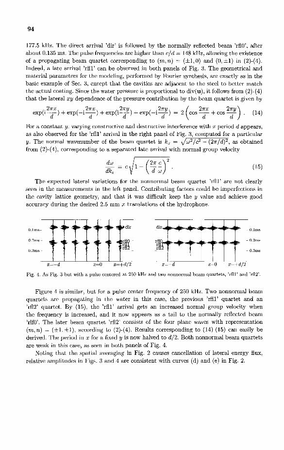
94
177.5 kHz. The direct arrival 'dir' is followed by the normally reflected beam 'rflO', after about 0.135 ms. The pulse frequencies are higher than c/d = 148 kHz, allowing the existence of a propagating beam quartet corresponding to (m,n) = (±1,0) and (0, ±1) in (2)-(4). Indeed, a late arrival 'rfll' can be observed in both panels of Fig. 3. The geometrical and material parameters for the modeling, performed by Fourier synthesis, are exactly as in the basic example of Sec. 3, except that the cavities are adjacent to the steel to better match the actual coating. Since the water pressure is proportional to div(u), it follows from (2)-(4) that the lateral xy dependence of the pressure contribution by the beam quartet is given by
,.2nx. .2irx. ,.2ny. . 27ry. e x p ( i — ) + e x p ( - i — ) + e x p ( i — ) + e x p ( - i — )
2-rrx 2iry\ , . • _ + « » - * ) . (14)
For a constant y, varying constructive and destructive interference with x period d appears, as also observed for the 'rfll' arrival in the right panel of Fig. 3, computed for a particular y. The normal wavenumber of the beam quartet is kz = ^/w2/c2 — (2n/d)2, as obtained from (2)-(4), corresponding to a separated late arrival with normal group velocity
du
dkz
2it C
d w (15)
The expected lateral variations for the nonnormal beam quartet 'rfll' are not clearly seen in the measurements in the left panel. Contributing factors could be imperfections in the cavity lattice geometry, and that it was difficult keep the y value and achieve good accuracy during the desired 2.5 mm x translations of the hydrophone.
£=—d x=0 x=+d/2 x=—d x=0 x=+d/2
Fig. 4. As Fig. 3 but with a pulse centered at 250 kHz and two nonnormal beam quartets, 'rfll' and 'rfl2'.
Figure 4 is similar, but for a pulse center frequency of 250 kHz. Two nonnormal beam quartets are propagating in the water in this case, the previous 'rfll' quartet and an 'rf!2' quartet. By (15), the 'rfll' arrival gets an increased normal group velocity when the frequency is increased, and it now appears as a tail to the normally reflected beam 'rlfO'. The later beam quartet 'rfl2' consists of the four plane waves with representation (m,n) = (±1,±1) , according to (2)-(4). Results corresponding to (14)-(15) can easily be derived. The period in x for a fixed y is now halved to d/2. Both nonnormal beam quartets are weak in this case, as seen in both panels of Fig. 4.
Noting that the spatial averaging in Fig. 2 causes cancellation of lateral energy flux, relative amplitudes in Figs. 3 and 4 are consistent with curves (d) and (e) in Fig. 2.

95
5. Design of Anechoic Coatings
At lower frequencies, with only the normally reflected beam propagating in the water, Fig. 2 shows that an Alberich coating can provide significant echo reduction. Results of the same character have been given by Cederholm,4 who computed reflection coefficients as functions of frequency based on parameter matching to certain experimental data. Unfortunately, direct measurements of the anechoic properties cannot be presented in an open publication.
Anechoic coatings can be designed by numerical methods. The results obtained by two such methods, allowing certain variations to the basic example in Sec. 3, are shown as curves (d) and (e) in the left panel of Fig. 5. Curve (d) was obtained by differential evolution (DE) minimization. Simulating annealing and genetic algorithms have been popular global optimization methods during the last decade. DE is related to genetic algorithms, but the parameters are not encoded in bit strings, and genetic operators such as crossover and mutation are replaced by algebraic operations. For applications to underwater acoustics, DE has recently been claimed to be much more efficient than genetic algorithms12 and comparable in efficiency to a modern adaptive simplex simulated annealing algorithm.13
HR m / s > P3 VI l.Or ' J c ^ c '
0.5
O.Q[ m n ? ' .? 6 . ' 10 20 30 kHz 1450 1500 1550 1.25 2 3 4 5
Fig. 5. Left: Reflectancies as functions of frequency. Curves (a)-(c) are exactly as in Fig. 2, but for a restricted frequency interval. Curve (d) was obtained with DE to minimize the maximum reflectance in the band 15-30 kHz. Curve (e), obtained with the analytic design method of Sec. 5.1, exhibits a reflectance null at 22.5 kHz. Middle and right: ^-function characterizations of coating models with maximum 15-30 kHz band reflectance below -17 dB, jointly in terms of j>2,P3 (middle panel) and J>6,J>7 (right panel). The £^ level-curve values are 1,5,10,20,30,.., reaching 60 in the middle panel and 50 in the right panel. The two dashed arcs in the right panel represent cavity diameters of 2.7 mm (lower dashed arc) and 3.6 mm (upper dashed arc).
The objective function for the DE minimization was specified as the maximum reflectance in the frequency band 15-30 kHz. Starting from the basic example of Sec. 3, eight parameters, denoted Pi,P2,--,P8, were varied within a reasonable search space: rubber density [pi, 0.9-1.3 kg/dm3] and compressional-wave velocity [p2, 1450-1550 m/s], rubber shear-wave velocity [j?3, 70-150 m/s] and absorption [p4, 7-27 dB/wavelength], and lattice period \p$ = d, 7-20 mm], coating thickness \pe, 1.25-5 mm], cavity diameter [0.5mm+p7 • (p^—1.25mm)], outer coating thickness between water and cavities [0.75mm+P8-(P6—1.25mm) ]. The parameters P7,p$ were defined as fractions, with nonnegative values such that pr + ps < 1.
An echo reduction of at least 17.5 dB can be achieved throughout the band 15-30 kHz, as seen to the left in Fig. 5, curve (d). The corresponding rubber parameters are p i = 0.90 kg/dm3 , p2 = 1455.3 m/s, ps = 149.8 m/s, p 4 = 26.9 dB/wavelength. The optimal geometrical parameters are p$ = d = 14.9 mm, pe = 4.98 mm, and p~t = 0.76, p% = 0.01. Improved echo
10
20
^ % r «
-
\^L^^^ \i&f \ ( e ) / . .
LOU
100
Tf\ m/s, j>2

96
reduction could be obtained by also varying the rubber compressional-wave absorption. Some 40000 coating models were tested at this DE optimization. More information is
contained in the search ensemble than just the optimal model. For example, let A be the set in the search space corresponding to coatings with maximum reflectance below -16.8 dB in the band 15-30 kHz, with characteristic function XA{PI,P2, --TPS)- Estimation is possible of certain dimensionless functions, generically denoted £4, of various parameters, such as
. / x {nidP2dPz) • IIJIIIxA(pi,P2,-,P8)dpidpidp5dp6dp7dp8
IIIIIIIS XA(PI,P2, -,PS) dpidp2dp3dpidp5dp6dp7 dp&
for the parameters P2 and P3, where each integral involves the whole corresponding search-space cross-section. Estimates directly based on the DE search ensemble may be misleading, however, since the DE sampling is typically biased with an unknown sampling distribution.
For Bayesian inverse problems, Sambridge10 has proposed a resampling algorithm to estimate a posteriori probability density (PPD) function marginals. A neighborhood approximation10 to the PPD, from a DE search ensemble, for example, can easily be evaluated along lines in parameter space. The new ensemble is constructed by random walks in directions parallel to the axes (Gibb's sampling), without further objective function calls.
Here, a neighborhood approximation to \A is specified, and the Sambridge algorithm is adapted to produce an accordingly resampled ensemble with some 200000 models. The function £A{P2,P3) from (16), with average 1, is subsequently estimated in a straightforward way. The result is shown in the middle panel of Fig. 5. Most of the favorable coatings have rubber compressional-wave velocities below 1500 m/s, reasonably close to the velocity in the water, and rubber shear-wave velocities above 120 m/s. Without the resampling, the ^-function diagram would have appeared differently with higher values up to the left, indicating a DE-sampling bias as compared to the desired sampling here, controlled by XA-
Characterization in terms of a similarly produced £4 function of pe and p7 is made in the right panel of Fig. 5. It is natural that thick coatings (large p$) are preferred, but additional low-reflectance coatings appear within a large part of the region of p6iP7-space with cavity diameters, 0.5mm+p7-(p6 — 1.25mm), between 2.7 and 3.6 mm. Diameter-dependent single-cavity resonances, as modulated by multiple-scattering effects, appear to be essential for the loss mechanism and the frequency dependence of the reflectance.
5.1. Designing vanishing reflectance at an isolated frequency
The second numerical design method is based on analytic function theory. It was used to produce curve (e) in the left panel of Fig. 5, with vanishing reflectance at 22.5 kHz.
For a constant rubber density p and a varying complex rubber shear-wave velocity (3, the normal plane-wave reflection coefficient for waves from the water, now denoted 1Z, is an analytic function of the shear modulus fi = pf32 of the rubber material. The analyticity allows zeroes of lZ{n) to be identified by numerical winding-integral techniques, whereby the argument variation of 1Z is determined around search rectangles in the ji plane. Adaptive splitting of these search rectangles is applied until exactly one zero is enclosed. The secant method is finally used to refine the estimate of an isolated zero.
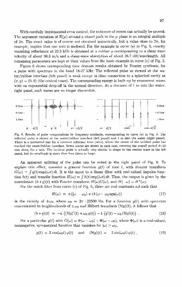
97
With carefully implemented error control, the existence of zeroes can actually be proved. The argument variation of H{n) around a closed path in the fj, plane is an integral multiple of 27r. The exact value is of course not obtained numerically, but a value close to 2w, for example, implies that one zero is enclosed. For the example in curve (e) in Fig. 5, exactly vanishing reflectance at 22.5 kHz is obtained at a rubber fi corresponding to a shear-wave velocity of about 98.3 m/s and a shear-wave absorption of about 26.7 dB/wavelength. All remaining parameters are kept at their values from the basic example in curve (c) of Fig. 2.
Figure 6 shows corresponding time domain results obtained by Fourier synthesis, for a pulse with spectrum in the band 18-27 kHz. The reflected pulse as viewed at the water/rubber interface (left panel) is weak except in close connection to a spherical cavity at (x, y) = (0, 0) (the central trace). The corresponding energy is built up by evanescent waves with an exponential drop-off in the normal direction. At a distance of 1 m into the water, right panel, such waves are no longer discernible.
0 .0ms-
0.5ms -
3 — 0.0ms
- 0.5ms
- 1.0ms
-d/2 =0 x=+d/2 x=-d/2 =0 =+d/2
Fig. 6. Results of pulse computations by frequency synthesis, corresponding to curve (e) in Fig. 5. The reflected pulse is shown at the water/rubber interface (left panel) and 1 m into the water (right panel). There is a horizontal line for a common reference time (zero), where the center of the incident pulse has reached the water/rubber interface. Seven traces are drawn in each case, covering the overall period rf=10 mm along the x axis. The incident pulse is actually very similar in shape to the central trace in the left panel, but its amplitude is more than four times as large.
An apparent splitting of the pulse can be noted in the right panel of Fig. 6. To explain this effect, consider a general function g(t) of time t, with Fourier transform G(u>) = / g(t) exp(iwi) dt. It is the input to a linear filter with real-valued impulse function h(t) and transfer function H(tv) = J h(t) exp(iwi) dt. Thus, the output is given by the convolution (h * g){t) with Fourier transform H{LS)G(LO), and H{—UJ) = H*(LS).
For the notch filter from curve (e) of Fig. 5, there are real constants a,b such that
H(w) « a (\ui\ — LOQ)+ib(u> — LUQsgn(uj)) (17)
in the vicinity of ±wo, where u>o = 2TT • 22500 Hz. For a function g(t) with spectrum concentrated to neighborhoods of ±WQ and Hilbert transform (TLg){t), it follows that
(h*g)(t) -a ([Hg)'{t)+u0g(t))-b(g'{t)-uQ{Hg){t)) . (18)
For a particular g(t) with G(u>) — $(o> — wo) + $(w + LOQ), where <E>(o;) is a real-valued, nonnegative, symmetrical function that vanishes for |w| > LJQ,
g(t) = 2 cos(u>ot) tp(t) and (Tig)(t) = — 2 sin(uiot) ip(t) (19)
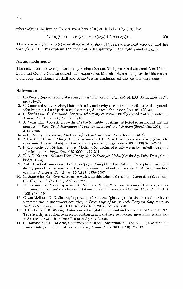
98
where tp(t) is t he inverse Fourier t ransform of $ ( w ) . It follows by (18) t h a t
(h*g)(t) « -2(p'(t) (-a sm(uJ0t) + b cos(uj0t)) . (20)
T h e modu la t i ng factor tp'(t) is small for small t, since tp(t) is a symmetr ica l function implying
t h a t </?'(0) = 0. This explains t he apparen t pulse spl i t t ing in t he right panel of Fig. 6.
A c k n o w l e d g m e n t s
T h e measurements were performed by Stefan Ban and Torbjorn Stahls ten, and Alex Ceder-
holm and G u n n a r Sundin shared their experience. Malcolm Sambridge provided his resam
pling code, and H a n n a Gothal l and R u n e West in implemented the opt imizat ion codes.
R e f e r e n c e s
1. H. Oberst, Resonant sound absorbers, in Technical Aspects of Sound, ed. E.G. Richardson (1957), pp. 421-439.
2. G. Gaunaurd and J. Barlow, Matrix viscosity and cavity-size distribution effects on the dynamic effective properties of perforated elastomers, J. Acoust. Soc. Amer. 75 (1984) 23-34.
3. H. Strifors and G. Gaunaurd, Selective reflectivity of viscoelastically coated plates in water, J. Acoust. Soc. Amer. 88 (1990) 901-910.
4. A. Cederholm, Acoustic properties of Alberich rubber coatings subjected to an applied ambient pressure, in Proc. Tenth International Congress on Sound and Vibration (Stockholm, 2003), pp. 2515-2522.
5. J. B. Pendry, Low Energy Electron Diffraction (Academic Press, London, 1974). 6. Z. Liu, C. T. Chan, P. Sheng, A. L. Goertzen and J. H. Page, Elastic wave scattering by periodic
structures of spherical objects: theory and experiment, Phys. Rev. B 62 (2000) 2446-2457. 7. I. E. Psarobas, N. Stefanou and A. Modinos, Scattering of elastic waves by periodic arrays of
spherical bodies, Phys. Rev. B 62 (2000) 278-291. 8. B. L. N. Kennett, Seismic Wave Propagation in Stratified Media (Cambridge Univ. Press, Cam
bridge, 1983). 9. A.-C. Hladky-Hennion and J.-N. Decarpigny, Analysis of the scattering of a plane wave by a
doubly periodic structure using the finite element method: application to Alberich anechoic coatings, J. Acoust. Soc. Amer. 90 (1991) 3356-3367.
10. M. Sambridge, Geophysical inversion with a neighbourhood algorithm - 2 appraising the ensemble, Geophys. J. Int. 138 (1999) 727-746.
11. N. Stefanou, V. Yannopapas and A. Modinos, Multem2: a new version of the program for transmission and band-structure calculations of photonic crystals, Comput. Phys. Coram. 132 (2000) 189-196.
12. C. van Moll and D. G. Simons, Improved performance of global optimisation methods for inversion problems in underwater acoustics, in Proceedings of the Seventh European Conference on Underwater Acoustics, ed. D. G. Simons (Delft, 2004), pp. 715-720.
13. H. Gothall and R. Westin, Evaluation of four global optimisation techniques (ASSA, DE, NA, Tabu Search) as applied to anechoic coating design and inverse problem uncertainty estimation, M.Sc. thesis, Swedish Defence Research Agency (2005).
14. S. Ivansson and I. Karasalo, Computation of modal wavenumbers using an adaptive winding-number integral method with error control, J. Sound Vib. 161 (1993) 173-180.

SEISMIC CHARACTERIZATION AND MONITORING OF THIN-LAYER RESERVOIR
LONG JIN*, XIAOHONG CHEN, JINGYE LI
China Petroleum University (Beijing), China
jinlong@cup. edu. en
Thin-layer reservoir has great significance for oil exploration and development. Seismic
characterization and monitoring of thin-layer reservoir has spatial advantage. New
seismic attributes and attributes combination analysis are proposed, including attributes
versus incidence angle, attributes versus scale, reflection coefficient spectrum and time-
frequency analysis for detailed thin-layer reservoir characterization.
1 Introduction
Thin-layer reservoirs are large in north china and other areas in the world.
It is also an important research topic for geophysicists. With the
development of oil exploration, detailed analysis of thin-layer reservoir is
needed.
Many researchers have done important work in this area. Widess studied
amplitude character of thin-layer using normal pulse reflections[l]. Lange,
Rafipour and Marfurt studied seismic attributes for thin-layer and fluid
discrimination^][3][4]. Christopher and James analyzed the effect of the
converted wave and multiple on thin-bed and AVO modeling [5] [6]. Chung
analyzed the precision of different approximation[7]. Liu studied the
amplitude attributes for thin-layer using acoustic wave equation modeling
method[8]. Ellison studied the modeling and analysis method for thin-layer
reservoir monitoring [9].
We studied new attributes and attributes combinations for thin-layer
reservoir characterization and monitoring.
99

2 Thin-layer seismic modeling
Many author using convolution based modeling method in thin-layer
studies[l][5]. Reflectivity method can also be used[6]. We use a method
similar to that used by Liu[8], but our method is based on elastic equation.
There is no analytical expression for these method. Detailed derivation is
in appendix. Figure 1 is the modeling result for a simple model with only
three layers.
J I_J—j_J J 1 , J 1 , L _ i _ i . l__l L 1 J L_ 0 500 1000 1500 2000
OffsetCm)
Figure 1 Seismic modeling result for a simple model with three layers
3 Seismic attributes versus incidence angle for thin-layer
AVO has been widely used in oil exploration. Mazzotti also proposed the
combined amplitude, phase and frequency versus offset analysis for
layered bed[10]. We use this method in thin-layer reservoir analysis.
Three layer model is studied. The upper and lower layer are both shale and
the middle layer is sand. The rock properties for the model is in table 1,
which is excerpted from [11]. The thickness of the middle layer can be
changed. Later experiment is also based on this data. Figure2-Figure5 is
amplitude and phase versus incidence angle for the three models when bed

101
thickness change. Conventional analysis used only amplitude. Our studies
show that phase can help separate different thickness of the bed. Figure6 is
amplitude and phase versus incidence angle for velocity change. There are
good correlation between amplitude, phase versus incidence angle and
velocity change.
Table 1 rock properties used for the synthetic seismograms
Shale
Sandl
Sand2
Sand3
Vp(m/s)
3900
3855
3597
3755
Vs(m/s)
2086
2202
2217
2254
P (g/cc)
2.300
2.320
2.288
2.192
Sw
1
0.8
0.2
0 S 10 15 20 23 30 36 40 45 50
incidence angle
(a)
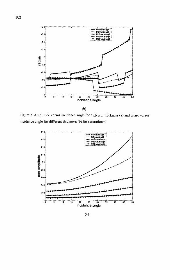
102
IS 30 25 30 35
incidence angle
(b)
Figure 2 Amplitude versus incidence angle for different thickness (a) and phase versus
incidence angle for different thickness (b) for saturation=l
1S 30 25 30 35
incidence angle
(a)

103
incidence angle
(b)
Figure 3 Amplitude versus incidence angle for different thickness (a) and phase versus
incidence angle for different thickness (b) for saturation=0.8
0 s i 1 i ; s j i j . j 0 5 10 1S 20 25 30 35 40 45 50
incidence angle
(a)

104
> S i ! i k 1 J 1 3
"0 5 10 15 20 25 30 35 40 45 SO
incidence angle
(b)
Figure 4 Amplitude versus incidence angle for different thickness (a) and phase versus
incidence angle for different thickness (b) for saturation=0.2
0 5 10 15 20 25 30 35 40 45 50
incidence angle
(a)

15 20 25 30 35
incidence angle
(b)
Figure 5 Amplitude versus incidence angle for different velocity change (a) and phase
versus incidence angle for different velocity change (b) for saturation =1 and
thickness=0.25 wavelength
• 0% velocity change ' l ^ve toc f ly change • 2% velocity change
3% velocity change > 4%vsJoc% change
15 JO 25 30 35
incidence angle
(a)
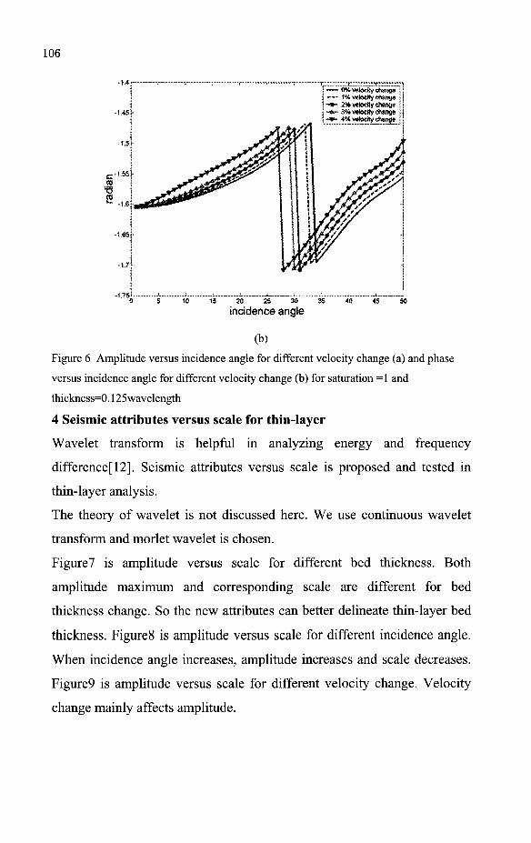
—— 0% velocity change — 1 % velocity change - • - 2 % velocity change -*>~ 3% veloctty change -**_4%vetocaychange
- -1 .S5 -
00
-1.65
« 15 30 25 30 35 40 45 50
incidence angle
(b)
Figure 6 Amplitude versus incidence angle for different velocity change (a) and phase
versus incidence angle for different velocity change (b) for saturation =1 and
thickness=0.125wavelength
4 Seismic attributes versus scale for thin-layer
Wavelet transform is helpful in analyzing energy and frequency
difference[12]. Seismic attributes versus scale is proposed and tested in
thin-layer analysis.
The theory of wavelet is not discussed here. We use continuous wavelet
transform and morlet wavelet is chosen.
Figure7 is amplitude versus scale for different bed thickness. Both
amplitude maximum and corresponding scale are different for bed
thickness change. So the new attributes can better delineate thin-layer bed
thickness. Figure8 is amplitude versus scale for different incidence angle.
When incidence angle increases, amplitude increases and scale decreases.
Figure0- is amplitude versus scale for different velocity change. Velocity
change mainly affects amplitude.

Scale
(a)
(b)
Figure7 Amplitude versus scale for different bed thickness when incidence
angle is 0 (a) and Amplitude versus scale for different bed thickness when
incidence angle is 30(b).

Scale
(b)
Figure8 Amplitude versus scale for different incidence angle when bed
thickness is 1/4 wavelength (a) and Amplitude versus scale for different
incidence angle when bed thickness is l/8wavelength (b).

Scale
(a)
0 10 20 30 40 ao 60 TO
Scale
(b)
Figure9 Amplitude versus scale for different velocity change when bed
thickness is 1/4 wavelength (a) and Amplitude versus scale for different
velocity change when bed thickness is l/8wavelength (b).

5 Reflection coefficient spectrum for thin-layer thickness and velocity
change
Spectral decomposition has been successfully used in bed thickness
estimation and fluid discrimination[13][14]. The basis of spectral
decomposition is reflection coefficient spectrum dependence on thickness
and velocity change. Using reflection coefficient spectrum, thickness and
velocity change can be separated in thin-layer. Figure 10-11 is reflection
coefficient spectrum for different bed thickness and different velocity
change. Bed thickness mainly affect frequency of reflection coefficient
spectrum maximum. Velocity change mainly affect amplitude of reflection
coefficient spectrum maximum. Using these two attributes, the bed
thickness and velocity change can be discriminated.
(a)
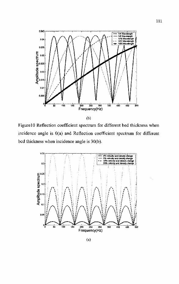
I l l
(b)
Figure 10 Reflection coefficient spectrum for different bed thickness when
incidence angle is 0(a) and Reflection coefficient spectrum for different
bed thickness when incidence angle is 30(b).
Frequency{Hz)
(a)
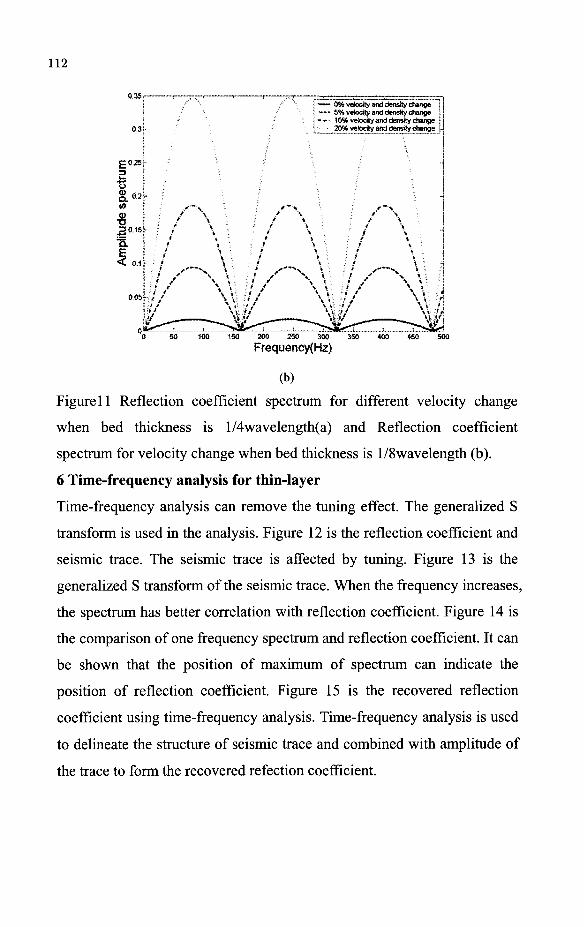
112
0,3 - 20% velocity artf densfty cjiange }.
(b)
Figure 11 Reflection coefficient spectrum for different velocity change
when bed thickness is l/4wavelength(a) and Reflection coefficient
spectrum for velocity change when bed thickness is l/8wavelength (b).
6 Time-frequency analysis for thin-layer
Time-frequency analysis can remove the tuning effect. The generalized S
transform is used in the analysis. Figure 12 is the reflection coefficient and
seismic trace. The seismic trace is affected by tuning. Figure 13 is the
generalized S transform of the seismic trace. When the frequency increases,
the spectrum has better correlation with reflection coefficient. Figure 14 is
the comparison of one frequency spectrum and reflection coefficient. It can
be shown that the position of maximum of spectrum can indicate the
position of reflection coefficient. Figure 15 is the recovered reflection
coefficient using time-frequency analysis. Time-frequency analysis is used
to delineate the structure of seismic trace and combined with amplitude of
the trace to form the recovered refection coefficient.

113
4) !
" o i — f L c o:
g-0.5 0) 0= 9)
-if- T~^7 0 0.02 0,04 O.06 0.08 0,1 0.12 0,14 0.16 0.18 0.2
time
Figure 12 Simple reflection coefficient and seismic trace
100 ISO
frequency
Figure 13 Spectrum for the modeled seismic trace

i; S05i
•S-osi-^ i !f= I <5) I •--1.5
T 1
O 0.02 0.04 0.06 0,08 0.1 0,1! 0.14 0.16 0.18 0.2
time
Figure 14 Comparison of reflection coefficient and one high frequency spectrum
<§j"2o b.oT~~oo4"™"o.o6 ooe 0.1 o,u 0.14 0.16 0.18 0.2
H-^T-
Figure 15 comparison of recovered reflection coefficient and true reflection
coefficient
7 Conclusions and discussions
The thin-bed seismic signature is affected by both bed thickness and
reservoir property change. Using the proposed seismic attribute or

combination analysis method, thin-bed reservoir can be characterized and
monitoring more precisely.
Acknowledgement
Thank my friend Chen tiansheng for his help in thin-layer seismic
modeling.
Reference
1 Widess, M.B., How thin is a thin bed?: Geophysics, 1973, 38:1176-1180.
2 James N. Lange, H. A. Almoghrabi., Lithology discrimination for thin
layer using wavelet signal parameters.:Geophysics, 1988, 53:1512-1519.
3 B. Rafipour, E. Herrin. Phase offset indicator(POI): A study of phase
shift versus offset and fluid content.:Geophysics, 1986, 51:679-688.
4 K. J. Marfurt, R. L. Kirlin. Narrow-band spectral analysis and thin-bed
tuning. Geophysics, 2001, 66:1274-1283.
5 Christopher Juhlin, Roger Young. Implication of thin layers for
amplitude variation with offset(AVO) studies.: Geophysics, 1993,
58:1200-1204.
6 James L. Simmmons, Jr, Milo M. Backus. AVO modeling and the
locally converted shear wave. Geophysics, 1994, 59:1237-1248.
7 Chung, H. M., Lawton, D. C. Amplitude responses of thin beds:
Sinusoidal approximation versus Ricker approximation: Geophysics, 1995,
223-230.
8 Yinbin Liu and Douglas R.Schmitt. Amplitude and AVO responses of
single thin bed.: Geophysics, 2003, 68(4): 1161 -1168.
9 Shelley J. Ellison, Matthias G. Imhof, Cahit Coruh, etc. Modeling offset-
dependent reflectivity for time-lapse monitoring of water-floor production
in thin-layer reservoir.: Geophysics, 2004, 69:25-36.
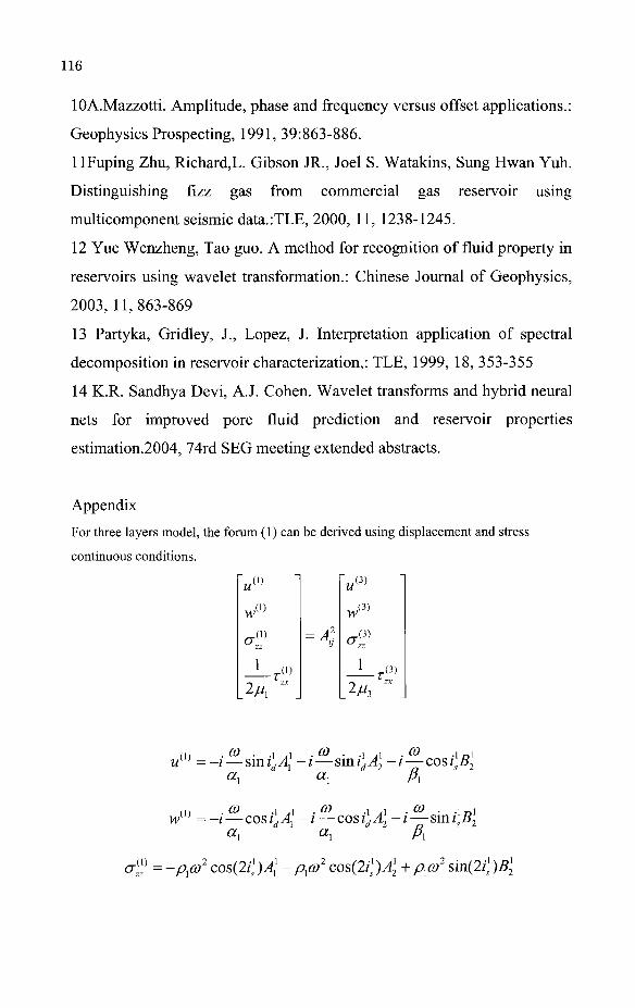
lOA.Mazzotti. Amplitude, phase and frequency versus offset applications.:
Geophysics Prospecting, 1991, 39:863-886.
1 lFuping Zhu, Richard,L. Gibson JR., Joel S. Watakins, Sung Hwan Yuh.
Distinguishing fizz gas from commercial gas reservoir using
multicomponent seismic data.:TLE, 2000, 11, 1238-1245.
12 Yue Wenzheng, Tao guo. A method for recognition of fluid property in
reservoirs using wavelet transformation.: Chinese Journal of Geophysics,
2003, 11,863-869
13 Partyka, Gridley, J., Lopez, J. Interpretation application of spectral
decomposition in reservoir characterization,: TLE, 1999, 18, 353-355
14 K.R. Sandhya Devi, A.J. Cohen. Wavelet transforms and hybrid neural
nets for improved pore fluid prediction and reservoir properties
estimation.2004, 74rd SEG meeting extended abstracts.
Appendix
For three layers model, the forum (1) can be derived using displacement and stress
continuous conditions.
"M(1)
w(,)
°T 1 r«>
,-» zx
_2M
= 4
V3 )
w(3)
^
1 r o , /-I ZX
u ' =-i — smidAl -i—smidA2-i — cosisB2 ax ax (3X
w(> =-i — cos idA{-i— cosidA2-i—smisB2 ax ax f3x
aM = -P{0)2 cos(2r')41 - px0)2 cos{2is)A[ + A » 2 sin(2/])^

1 m CO1 . , ., ,, CO2 . , ., ,, CO T(£ = sin i\ cos i\A\ + — s i n i\ cos i\A\ + —— cos(2/s
1 )B\ 2ju{ or, or, 2p,
(3) • &> . .3 ,3 . #? .3 n 3
-P' - - ? — s i n / J 4 -z — cos/^5, a 1 0
«"3 /"3
<y .3 j 3 . &> COSJ, A -I
a 1 /5
«3 A
(3) • <" -3 ^3 . w . .3 n 3
w w = - i — c o s J ^ , - z — sinisBx "3 ^ 3
°"i3) = - A ' 9 ' cos(2zs3)43 + p3<y2 sin(2/s
3)513
1 m CO . .3 .3 ,3 CO n -^ = - ^ s i n / 3 cos/343
+ - _ c o s ( 2 / 3 ) 5 13 (l)
2//3 a3 2p3
Where or, % /?, and or3 > /?3 is the p and s wave velocity. is* id% /J% Zrf are angle
of refection s wave, reflection p wave, transmission s wave, transmission p wave.
A^ A2s B2S Ax^ flj is the displacement amplitude of incidence p wave, reflection p
wave, reflection s wave, transmission p wave, transmission s wave.
The ratio of displacement amplitude can be defined as,
T =^L^L (2)
Where, R is reflection coefficient in frequency domain.
H PP 4 A
B\ or, R = - f— " 4 A
/' pp
A] or,
A' a3


THE ENERGY-CONSERVING PROPERTY OF THE STANDARD PE
DING LEE
Naval Undersea Warfare Center, Newport, RI, USA
ER-CHANG SHANG
CIRES, University of Colorado, Boulder, Colorado, USA
December 19, 2005
In 1974 a model was introduced by Frederick D. Tappert for predicting long-range wave propagation in a range-dependent environment. He applied the parabolic Equation approximation to transform the Helmholtz equation into a parabolic equation, the very first Parabolic Equation (PE). A pressure-release surface boundary is considered along with an artificial bottom boundary treatment. This paper proved that the Tappert model is energy-conserving.
1. Introduction
Over the past quarter century, the authors had continuous technical interactions with Frederick D. Tappert who, in 1974, introduced a model which is to apply the parabolic equation approximation to transform the Helmholtz equation into a parabolic equation, the very first parabolic equation (PE). In 1984 the first author invited Tappert to spend a summer together to do research in relation to PE developments. The author raised a question to Tappert: You made a big contribution of PE to the acoustic community; in order to honor your contribution, should the very first PE be named after you? Tappert said: No, but suggested naming it the Standard PE. From that time on the Standard PE was recognized by the acoustics community.
The Standard PE is a 2-dimensional (range and depth) representative wave equation which defines an initial-boundary value problem. Associated with the Standard PE, the surface boundary condition is considered pressure-release; the bottom boundary condition is treated by a special technique, introduced by Tappert, called "artifical bottom". The artifical bottom technique is to extend the field vertically down to the bottom deep enough such that u(r, z) = 0 at the bottom. The Standard PE to go with the assumed boundary conditions is regarded as the Tappert model.
119

120
Since the early 1980's, the authors and Tappert continued their technical discussions including the issues, contributions, and new results with reference to the PE-related developments. Various topics were among their discussions; Standard PE was one of the topics we discussed, but the energy-conserving issue entered the discussions but we did not pursue to prove that the Tappert model is energy-conserving. This paper is to prove that the Tappert model is energy conserving.
2. Basic Development
This section consists of the outline of two parts: The theoretical development of the standard PE and the associated surface and bottom boundary conditions. Theoretical details can be found in references [1, 2].
2.1. The standard PE
Let r be the range variable, z be the depth variable, u(r, z) the 2-dimensional wave field, n(r, z) be the index of refraction which is a real-valued function, and ko is the reference wavenumber which is a real-valued scalar.
The very first Parabolic Equation introduced by Tappert [1] takes the form:
iko , 0, , H. 1 d2u
Ur = -{n*(r,z)-l)*+—-^. (2.1)
2.2. Associated boundary conditions
Two types of boundary conditions are considered: the surface and the bottom boundaries. Let zs indicate the surface boundary and z&, the bottom boundary.
2.2.1. The surface boundary condition
The assumed pressure-release surface condition indicates that u(r,zs) = 0. The indication implies that the prescribed surface boundary conditions are
du du u(r.zs) = 0, u(r,z,) = 0, 7H*. = 0 - 7 T ^ = ° - (2 '2)
az oz
2.2.2. The bottom boundary condition
A technique was introduced by Tappert to generate the bottom boundary condition. This technique is known as the "artificial bottom" which is to extend the wave field vertically deep enough such that u(r, zb) = 0 there. Therefore; the prescribed bottom boundary conditions are
uu ou u(r,zb)=0, u(r,zb) = 0, ^ L = < > > ^ U = °'• (2-3)

121
3. Energy-Conserving Property
Writing Eq. (2.1) in the form
ur = a(n2(r, z) — \)u + buz
where ik0
From Eq. (3.1),
we have
and
Then
a = — i b = „ , . 2 2ik0
ur = a(n2(r.z) — l)u + b
uru = a(n2(r, z) — l)uu + b
d2u
dz*
— - , 2/ \ -.s- T fd2U . iru = a{n (r.z) — \)uu + b I —— J u
uru + uru =
We want to examine whether or not
d2u d2i dz2
u d2
u £ W = 1(\U\>).
(3.1)
(3.2)
(3.3)
(3.4)
(3.5)
(3.6)
dr \u\zdz = 0.
Making use of expressions in Eq. (3.6), we have
dr
fZb r) fz d2u\_ fd2u\ ' dz.
(3.7)
(3.8)
Then, saving of the writing of ^ and the constant b, the first integral of the right-hand-side of Eq. (3.8) can be evaluated by means of integration by parts; i.e.
/
Zb /d2u\_1 (dus du\ . r-dudu, , x
Tzn--LTzd-zdz- (3'9)
Similarly, the second integral of the right-hand-side of Eq. (3.8) becomes
/
czb /oa-
( ^ ) UdZ du\ . fdu\ . fZbdudu, dz~)uU+{dz')uL+ I -~^T~dz- (3-10) dz dz

122
The term (§^)w|Zs in Eq. (3.9) and the term ( | j )u | 2 s in Eq. (3.10) all go to zero due to the surface boundary condition, (2.2).
Similarly, the term {%)u\Zb in Eq. (3.9) and the term ( f f H 2 „ in Eq. (3.10) all go to zero due to the bottom boundary condition, (2.3), therefore;
d fz\ ,2, d A [Zb f du9a\ , fZbdudUl] n . „ ,
Then, the energy-conserving property of the standard PE with the prescribed boundary conditions, (2.2) and (2.3), is proved.
4. Remarks
The Standard PE is a two-dimensional model with a narrow angle capability. These days the three-dimensional models have become more realistic in real applications. Not many users in the scientific community are using the two-dimensional model. Why bother to study the energy-conserving property for the Standard PE?
There are a few answers for this question:
1. Because of the interest in three-dimensional problems, the Standard PE may not be used often in the acoustics community, to report this theoretical result to the public, we believe, may still interest the readers.
2. We selected the Tappert model to show it is energy-conserving, on the other hand, is to remember the late Tappert for what he did for the scientific community.
3. The technique, we used to examine the energy-conserving property, can be used to examine the energy-property of other PE models.
5. Conclusion
The PE influence to the acoustic community is huge. All further-developed PE's are in use widely in the acoustifics community; they were all derived from the standard PE which benefited the scientific community a great deal. The Standard PE, even now-a-days is having limited use, it must not be forgotten; interestingly, the energy-conserving property of the Tappert model should not be unmentioned. This procedure may be applied to investigate the energy-conserving property for all other PE's, PE-like models, or other types of wave propagation models.
5.1. Dedication
The impact of the PE to the scientific community is huge. In recognition of the PE contribution to the acoustic community, we cannot forget the Standard PE; and Frederick D. Tappert must be remembered. This paper is written in memory of our long time colleague Frederick D. Tappert.

123
Acknowledgments
This research of the first author was supported by the U.S. Naval Undersea Warfare
Center (Newport) Independent Research project.
R e f e r e n c e s
1. Tappert, F. D., The Parabolic Equation Approximation Method, in Wave Propagation and Underwater Acoustics, ed. J. B. Keller and J. S. Papadakis, Lecture Notes in Physics 70, Springer-Verlag, Heidelberg, 1977, 224-287.
2. Lee, D. and S. T. McDaniel, BOOK. 3. Lee, D., A. D. Pierce, and E. C. Shang, Parabolic Equation Development in the
Twentieth Century, J. Corny. Acoist. 8(4), 2000, 527-628.

A Dedication to Professor Tappert
Professor Frederick D. Tappert, who introduced the parabolic equation approximation to the acoustic community, passed away in 2001.
Professor Michael I. Tarodakis and Dr. Finn B. Jensen organized a special memorial session for Prof. Tappert at the 6th International Conference on Theoretical and Computational Acoustics (ICTCA) at Hawaii, Honolulu, U.S.A. August 11-15, 2003.
Professor Tarodakis and Dr. Jensen further encouraged the session speakers to contribute their articles to be included in the Proceedings of Theoretical and Computational Acoustics 2003. Their efforts in organizing this memorial session is appreciated by all of us.
In January, 2000,1 visited Prof. Tappert in Miami, Florida, U.S.A. He expressed interest in contributing a paper to the 6th ICTCA. At that time, I started writing a paper on Revolutionary Influence of the Parabolic Equation Approximation to honor him. I continued to make progress on this article. At that stage, it was an article but, I left room for expansion. After the shocking news regarding Prof. Tappert, I immediately started writing another article entitled The Energy-Conserving Property of the Standard PE and dedicated it in memory of Prof. Tappert. Suddenly I was diagnosed with age-related Macular Degeneration. I had difficulty reading and writing. I was forced to stop writing this article, which I had planned to submit at the 2003 Hawaii ICTCA in the memorial session for Prof. Tappert, organized jointly by Prof. Tarodakis and Dr. Jensen. I was unable to submit the Energy Conserving paper on time. I felt very guilty for not being able to present this paper. After the conference, I was determined to complete writing this article, if possible. Prof. Er-Chang Shang came to help. With his help, this article has been completed. I thank Prof. Shang for his help and thank the committee chairs for giving me the opportunity to present this article at the 2005 Hangzhou ICTCA.
Professor Frederick D. Tappert has gone; his PE contribution will be remembered. This article is dedicated in memory of my long-time colleague, Frederick D. Tappert.
Ding Lee
124

Fredrick D. Tappert April 21, 1940 - January 9, 2001
Frederick D. Tappert was born April 21, 1940 in Philadelphia, Pennsylvania. His parents, the Reverend Dr. Theodore G. Tappert and Helen Louise Carson Tappert, raised their family of four children in the Lutheran Theological Seminary in Philadelphia, where the Reverend Dr. Tappert was a noted theologian. Fred showed an early penchant toward mathematics and science and attended Central High School in Philadelphia, which recognized outstanding young men in this area. From there he went on to study engineering at Penn State University, funded by the Ford Foundation, where he graduated with a B.S. in Engineering Science with honors in 1962. Fred went on to pursue his Ph.D. in theoretical physics from Princeton University with a full scholarship from the National Science Foundation. He earned his Ph.D. in 1967.
Upon graduation Dr. Tappert was hired to the Technical Staff at Bell Laboratories in Whippany, New Jersey from 1967 - 1974, where he worked on plasma physics and high altitude nuclear effects, UHF radar propagation, solitons in optical fiber, and ocean acoustic surveillance systems. He left Bell Labs and became a Senior Research Scientist at the Courant Institute, at New York University from 1974 - 1978, where he performed research on controlled fusion and nonlinear waves, as well as ocean acoustics. It was at the Courant Institute that Fred first realized the impact that he could have upon students and thus his future took on even more meaning as the great professor and advisor began to emerge in Fred.
Fred realized his potential as an educator and scientist when he left the Courant Institute and joined the faculty at the University of Miami's Rosenstiel School for Marine and Atmospheric Science in August 1978. At RSMAS he taught graduate courses in ocean acoustics, occasional undergraduate courses in physics, and supervised the research of more than 25 awardees of M.S. and Ph.D. degrees. In addition, Professor Tappert carried out a vigorous program of sponsored research in the areas of ocean acoustics, and wave propagation theory and numerical modeling.
Dr. Tappert was a major participant in the ONR-sponsored initiative on "Chaos and Predictability in Long Range Ocean Acoustics Propagation." In this research he applied a recently developed 4-D (three space dimensional plus time) full-wave fully range-dependent parabolic equation (PE) ocean acoustic model to determine the limits of predictability of sound propagation and scattering. Since Dr. Tappert's most cited research was the original development of the PE numerical model, and he was also one of the originators of the concept of "ray chaos" in ocean acoustic propagation, this was a natural evolution for his research. Previously, Professor Tappert was a major participant in the ONR-sponsored "Acoustic Reverberation Special Research Project," the goal of which was to gain a scientific understanding of long-range low-frequency ocean surface and bottom reverberation by comparing numerical model predictions to measured
125

126
acoustic data, taking into account high resolution environmental data. In that research Professor Tappert developed a PE model of bistatic reverberation, the predictions of which compared favorably with measurements.
In addition to his university research, Dr. Tappert was a consultant to many organizations involved in applied projects related to wave propagation theory and numerical modeling. This includes the DANTES project, sponsored by DARPA, in which he developed a novel technique call Broadband Matched Field Processing (BMFP) that localizes sources of acoustic transient signals using a back-propagation method.
In October 2001, Fred was awarded the Superior Public Service Award from the Office of Naval Research. It was at this time that he was undergoing the rigors of chemotherapy in hopes that he would have more time in his fight against pancreatic cancer. This recognition brought tremendous joy to Fred. Unfortunately, he succumbed to the cancer only three months later on January 9, 2002. In November 2002, he was also posthumously awarded the Pioneers in Underwater Acoustics Award by the Acoustical Society of America. His wife, Sally, and two sons, Andrew and Peter, were present in Cancun, Mexico, to receive this award in his honor.
Sally Tappert

ESTIMATION OF ANISOTROPIC PROPERTIES FROM A SURFACE SEISMIC SURVEY AND LOG DATA
RUIPING LI, MILOVAN UROSEVIC
Department of Exploration Geophysics, Curtin University of Technology, Australia.
Routine P-wave seismic data processing is tailored for isotropic rocks. Such assumption typically works well for small incidence angles and weak anisotropy. However, in the last decade it has become clear that seismic anisotropy is commonplace. Moreover, its magnitude often severely violates the presumptions taken for routine processing. Consequently reservoir characterization may be significantly distorted by anisotropic effects. In particular the intrinsic shale (often sealing rock) anisotropy often has first order effect on AVO gradient. Hence an assessment of the shale properties from surface seismic data may be of the primary importance for quantitative interpretation. There are several inversion approaches which require full set of geological information. In reality we expect to have at least the log and surface seismic data available for such a task. We present here a newly developed hybrid inversion method which is suitable for the recovery of anisotropic parameters of sealing rocks under such conditions. The effectiveness of this approach was successfully tested on seismic data recorded in the North West Shelf, Australia.
1 Introduction
Inversion of surface seismic data for the elastic properties of sealing rocks can impact on the accuracy of the reservoir characterisation. Since shales, which are intrinsically anisotropic, comprise often sealing rocks, an inversion has to at least incorporate recovery of the full set of anisotropic parameters for a transversely anisotropic medium. The shale anisotropy and its variation across an oil or gas field could have first order effect on Amplitude Versus Offset-and-azimuth analysis (AVOaz) [6; 1]. An example incorporating weak shale anisotropy is shown in Figure 1. Shale anisotropy in this case affects reflectivity curve on moderate to far angles. This "deviation" of the reflectivity curve could potentially impact onto our ability to accurately predict fluid type and its distribution across the field. Thus it is clear that before attempting detailed analysis for reservoir properties it is highly desirable to analyze and determine the magnitude of the seal anisotropy. Consequently an assessment of the shale properties from surface seismic data may be of the primary importance for quantitative interpretation of reservoir rocks.
Thomsen [7] derived a convenient five-parameter model to describe seismic wave propagation in a transversely isotropic medium. There are many methods proposed to recover these elastic parameters, for example, the slowness surfaces method [2], the ray velocity field method from VSP surveys [4], the anisotropic moveout method from reflection events [8; 5]. Each of the above inversion method has been tested on field data sets separately provided enough information was available. However, we often have only surface seismic data and log data available for such inversion. In such case the existing methods fail to recover the elastic parameter accurately. For example the slowness method recovers the elastic parameters for an interval layer. The existence of a heterogeneous layer between successive receivers may produce errors in slowness surface determination. Deviation of the borehole, near surface inhomogeneities or topography of the surface also makes calculation of the slowness surfaces more
127
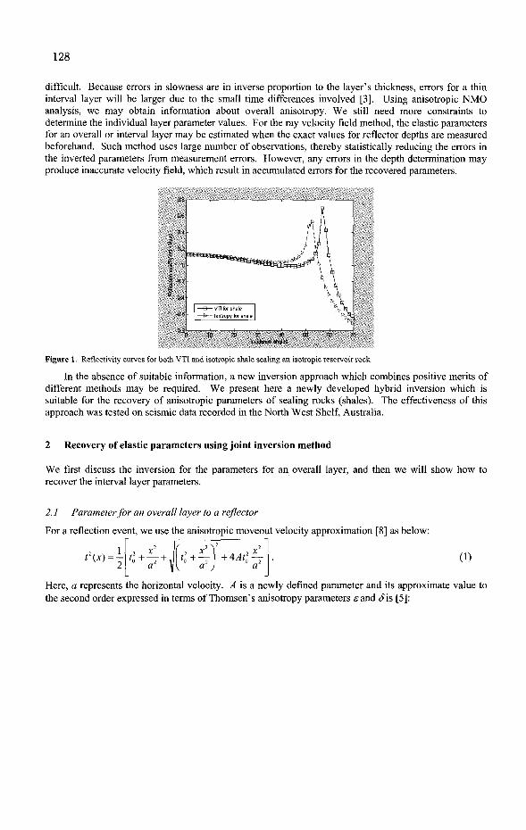
128
difficult. Because errors in slowness are in inverse proportion to the layer's thickness, errors for a thin interval layer will be larger due to the small time differences involved [3]. Using anisotropic NMO analysis, we may obtain information about overall anisotropy. We still need more constraints to determine the individual layer parameter values. For the ray velocity field method, the elastic parameters for an overall or interval layer may be estimated when the exact values for reflector depths are measured beforehand. Such method uses large number of observations, thereby statistically reducing the errors in the inverted parameters from measurement errors. However, any errors in the depth determination may produce inaccurate velocity field, which result in accumulated errors for the recovered parameters.
Incidence angles
Figure 1. Reflectivity curves for b-j\'A VTI and isotropic shale sealing an isotropic reservoir rock.
In the absence of suitable information, a new inversion approach which combines positive merits of different methods may be required. We present here a newly developed hybrid inversion which is suitable for the recovery of anisotropic parameters of sealing rocks (shales). The effectiveness of this approach was tested on seismic data recorded in the North West Shelf, Australia.
2 Recovery of elastic parameters using joint inversion method
We first discuss the inversion for the parameters for an overall layer, and then we will show how to recover the interval layer parameters.
2.1 Parameter for an overall layer to a reflector
For a reflection event, we use the anisotropic moveout velocity approximation [8] as below:
1 t2(x) = : tl+^\ +4At^ (1)
Here, a represents the horizontal velocity. A is a newly defined parameter and its approximate value to the second order expressed in terms of Thomsen's anisotropy parameters eand £is [5]:

129
A*2-(e-8)-{ 2 /
- i y + ( 3 + — )s2
If' -(4-y)«y. ( 2 )
Here, / = i-K with a0, /?<) are the vertical velocities for P and S-waves. To the first order
approximation, the A value is the double difference between the anisotropic parameters s and S, and A can be called as a dimensionless non-ellipticity parameter. The anisotropic velocity analysis which employs two-parameter (a and A) anisotropic semblance analysis is then implemented. For any set of parameter value of a and A, equation (1) is used to perform moveout corrections. The semblance coefficient Sc is then calculated. The values of the parameter a and A are determined for a specific reflection event when the semblance coefficients Sc achieves its maximum value Scmax.
When we have the exact values for the reflector depth and the vertical velocities, the anisotropic parameters e and Scan be determined from the recovered parameters a and A using equation (2). From the log data tied with the surface seismic data, the reflector depth and the vertical velocities may be estimated. However, due to the sensitivity of the anisotropy parameters, the accuracy for the inverted parameters sand Sis inadequate. For the surface seismic survey, the two-way-travel times (TWTs) with different offsets for a specific reflector can also be picked. When the depth of this reflector is known, the velocity values at different travel angles can be inferred. Hence, the ray velocity field method could be applied for the parameter recovery. Combining the above two methods, a hybrid inversion is developed by best-fitting the TWT field with constraints of the parameter a and A values from the anisotropic semblance analysis. Figure 2 gives the program flow for the hybrid inversion.
f Anise-tropic 3emblonces\ J2 ! !g iK f iSS*2LEf f iSJy i *E*^L i_J \ analysis Q, A /
__ }_»iCoimjutetrial.obsraved velocity fields]*"
/ Reflection two way travel time /— 'Compare the observed velocity'
fields w ith cilciilated field-,
~L__N ,
Output parameters
e.6
Figure 2. The program flow for the hybrid inversion technique using surface seismic and log data.
2.2 Parameter for an interval layer between two reflectors
This approach can be used to obtain apparent elastic parameters for several interfaces such as top and bottom of the shale layer or the top and bottom reservoir interfaces. The parameters e and S for the interval layer between these two interfaces are then determined from the measured TWTs for different offsets and the depth values for the interfaces by the ray velocity field method. Subsequently, the

130
slowness surface for this interval layer is built from the measured TWTs for different offsets and the layer thickness. The inverted interval parameters e and 8 from the ray velocity field method are then validated by best-fitting the slowness curves. Figure 3 shows the flowchart for the interval layer inversion program.
Inversion from the velocity fields above and below
the layer of interest
I Inversion from the slowness curves ;
\ J
Figure 3. The flowchart for the hybrid inversion technique for the interval layer properties.
The degree of the sealing rock anisotropy has significant effect on the AVOaz reservoir signature. Hence, the inverted anisotropic parameters for the top sealing rocks should play an important part in the reservoir characterization. In the following section, we apply our hybrid inversion to real field data.
3 Field data application
The hydrocarbon field analyzed is located in Exmouth Sub-basin, offshore North-West Shelf, Western Australia. High-quality cross-dipole sonic logs showed significant shear wave splitting (10-15%) over the reservoir interval. To utilize this information for reservoir rock characterization it was first necessary to estimate the anisotropy of the sealing shale and its effect on AVOaz signature.
For a CMP (common mid-point), the anisotropic semblance analysis [9] is applied along the time axis (t0). For each t0, the Sc values are computed for a set of a and A values. The parameters a and A are then determined when the semblance coefficient Sc hold its maximum value. Figure 4 shows an example for the reflection event at t0=2005 ms. The corresponding parameters are determined as: a=2452.5 m/s and A=0.16.
Along the seismic line, the parameter a and A are then determined using the above anisotropic semblance analysis. Figure 5 shows the parameter a and A values for different CMP for the same t0
value. The stability of the recovered parameters is demonstrated from the figures. At different t0, the Scmax values are then compared with the surface seismic section and the log data,
as shown in figure 6. The top shale layer is identified as the interval layer between two strong reflection events with local maximum Scmax values. The corresponding parameters a, A for the reflection events on the top and the bottom of the shale layer are also obtained through the anisotropic semblance analysis.
Output Barometers
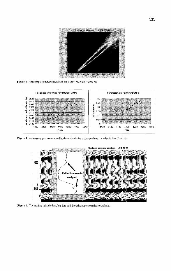
-Visrtropffi Semblancs ̂ otysis:2-3W ? C P M * «
Figure 4. Anisotropic semblance analysis for CMP=4185 at t(i=2005 ms.
131
Horizontal velocities for different CMPs
Jf 2520 • E. 2510 " 2500 « 2490 o 2480 > 2470 S 2460 0 2450 •c 2440 1 2430'- r ~~ '•
4180 4185 4190 4195 4200 4205 4210
CMP
Par
amet
er A
0.3
0.25
0.2
0.15
0.1
0.05
0 -. -4180
Parameter A for different CMPs
• * * *
. " . - « •
4185 4190 4195 4200 4205
CMP 4210
Figure 5. Anisotropy parameter ,4 and horizontal velocity a change along the seismic line (fixed to).
Surface seismic section Log data
Figure 6. The surface seismic data, log data and the anisotropic semblance analysis.
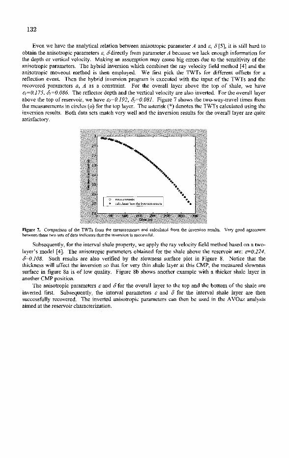
132
Even we have the analytical relation between anisotropic parameter A and s, 8 [5], it is still hard to obtain the anisotropic parameters e, 8directly from parameter^ because we lack enough information for the depth or vertical velocity. Making an assumption may cause big errors due to the sensitivity of the anisotropic parameters. The hybrid inversion which combines the ray velocity field method [4] and the anisotropic moveout method is then employed. We first pick the TWTs for different offsets for a reflection event. Then the hybrid inversion program is executed with the input of the TWTs and the recovered parameters a, A as a constraint. For the overall layer above the top of shale, we have £]=0.175, 8i=0.086. The reflector depth and the vertical velocity are also inverted. For the overall layer above the top of reservoir, we have s2=0.192, S2=0.081. Figure 7 shows the two-way-travel times from the measurements in circles (o) for the top layer. The asterisk (*) denotes the TWTs calculated using the inversion results. Both data sets match very well and the inversion results for the overall layer are quite satisfactory.
2.2
t 26
2.7
28,
measurements calculated from the inversion results
500 100D ISOCI 2000 2500 3000 3500 OUset (m)
Figure 7. Comparison of the TWTs from the measurements and calculated from the inversion results. between these two sets of data indicates that the inversion is successful.
Very good agreement
Subsequently, for the interval shale property, we apply the ray velocity field method based on a two-layer's model [4]. The anisotropic parameters obtained for the shale above the reservoir are: s=0.224, 8=0.108. Such results are also verified by the slowness surface plot in Figure 8. Notice that the thickness will affect the inversion so that for very thin shale layer at this CMP, the measured slowness surface in figure 8a is of low quality. Figure 8b shows another example with a thicker shale layer in another CMP position.
The anisotropic parameters s and 8 for the overall layer to the top and the bottom of the shale are inverted first. Subsequently, the interval parameters e and 8 for the interval shale layer are then successfully recovered. The inverted anisotropic parameters can then be used in the AVOaz analysis aimed at the reservoir characterization.

133
(a) Slowness surface for a thin layer (b) Slowness surface for a thick layer
Figure 8. The comparison of the slowness surfaces from the measurements and calculated from the inversion results.
4 Conclusions
From the log data and anisotropic semblance analysis, the reflection events at different two way travel times are analysed, as well as the horizontal velocities a and the anisotropic parameter A. From a seismic section, the two-way travel times for different offsets for a CMP location are manually picked. With the constraint of the parameter^ and horizontal velocity a values, a new hybrid inversion method is developed to recover anisotropic parameters e, S, reflector depth and the vertical velocity from the observations of two way travel times for different offsets. As the velocity field at different ray angles can be converted using the inverted reflector depth, verification procedure is carried out. The calculated values of TWT for different offsets using the recovered parameter values should coincide with the log measurements. Apparent differences between the measured and estimated values may suggest misfit of the seismic section with the log data.
After obtaining the apparent average parameter for the top and the bottom sealing layer or reservoir, the interval anisotropy parameters are obtained from the velocity field data using two-layer model approach [4]. From the travel time picks, the slowness surface for the interval layer is also constructed which allows us again to recover the interval anisotropy parameters. These two estimates should match each other.
The application of our new hybrid inversion methods to the field petroleum data suggests that the method is robust and should consequently result in reliable parameter estimates.
5 Acknowledgments
This is a project supported by the Curtin Reservoir Geophysics Consortium (CRGC). We thank CRGC for providing the field data. Thanks also go to Mr. Said Amiri Besheli for his help with the filed seismic data and log data.

134
6 References
1. Banik, N. C, An effective anisotropy parameter in transversely isotropic media: Geophysics, Soc. of Expl. Geophys., 52 (1987) pp. 1654-1664.
2. Hsu, K., Schoenberg, M. and Walsh, J. J., Anisotropy from polarization and moveout: 61st Ann. Internat. Mtg., Soc. of Expl. Geophys., (1991) pp. 1526-1529.
3. Kebaili, A., Le, L. H. and Schmitt, D. R., Slowness surface determination from slant stack curves, in Rathore, J. S., Ed., Seismic anisotropy: Soc. of Expl. Geophys., (1996) pp. 518-555.
4. Li R., Uren N. F., McDonald J. A. and Urosevic M., Recovery of elastic parameters for a multi-layered transversely isotropic medium: J. Geophys. Eng., 1 (2004) pp. 327-335.
5. Li R. and Urosevic M., Analytical relationship between the non-elliptical parameter and anisotropic parameters from moveout analysis: (2005) being prepared for publication.
6. Ruger, A., Variation of P-wave reflectivity with offset and azimuth in anisotropic media, 66th Ann. Internat. Mtg: Soc. of Expl. Geophys., (1996) pp.1810-1813.
7. Thomsen, L., Weak elastic anisotropy. Geophysics 51 (1986) pp. 1954- 1966. 8. Zhang, F. and Uren, N, Approximate explicit ray velocity functions and travel times for p-waves in
TI media: 71th Ann. Internat. Mtg., Soc. Expl. Geophys., Expanded Abstracts, (2001) pp. 106-109. 9. Zhang, F., Uren, N., and Urosevic, M., Anisotropic NMO corrections for long offset P-wave data
from multi-layered isotropic and transversely isotropic media: 73rd Ann. Internat. Mtg., Soc. Explor. Geophys., Expanded Abstracts, (2003) pp. 133-136.
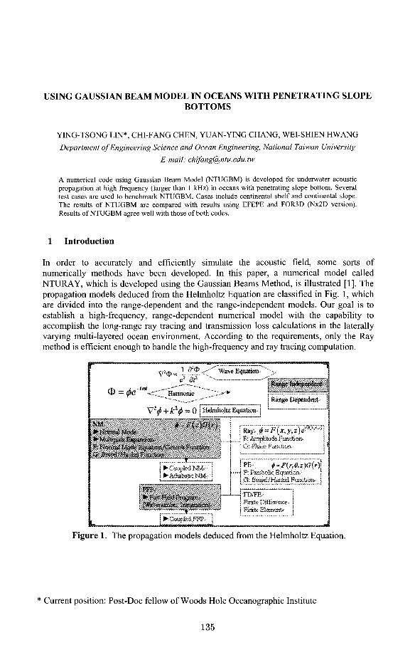
USING GAUSSIAN BEAM MODEL IN OCEANS WITH PENETRATING SLOPE BOTTOMS
Y I N G - T S O N G LIN*, C H I - F A N G C H E N , Y U A N - Y I N G C H A N G , W E I - S H I E N H W A N G
Department of Engineering Science and Ocean Engineering, National Taiwan University
E-mail: [email protected]
A numerical code using Gaussian Beam Model (NTUGBM) is developed for underwater acoustic propagation at high frequency (larger than 1 kHz) in oceans with penetrating slope bottom. Several test cases are used to benchmark NTUGBM. Cases include continental shelf and continental slope. The results of NTUGBM are compared with results using EFEPE and FOR3D (Nx2D version). Results of NTUGBM agree well with those of both codes.
1 Introduction
In order to accurately and efficiently simulate the acoustic field, some sorts of numerically methods have been developed. In this paper, a numerical model called NTURAY, which is developed using the Gaussian Beams Method, is illustrated [1]. The propagation models deduced from the Helmholtz Equation are classified in Fig. 1, which are divided into the range-dependent and the range-independent models. Our goal is to establish a high-frequency, range-dependent numerical model with the capability to accomplish the long-range ray tracing and transmission loss calculations in the laterally varying multi-layered ocean environment. According to the requirements, only the Ray method is efficient enough to handle the high-frequency and ray tracing computation.
f=-v $ -
1 f--el) Wave Equation
<D = <f>e c- (Jt
Humicmc
Ranjrc ln<icpun<!ciit
RdllJtC llL'pilull'Il!
NM
! ? I . • M I - ' U 1 :.«.-..!• : - H I -
\ !d> + kld = 0 Hflniholl/. liquation
0 - /•'(.-Jf/li ) Ray o~Flx.y,:)i' I": Amrtifji- .•''-r.--'i;;i
i I
"iT-'p" •.'.. : i y j »••:
PE 4-nr,0a)O(r)\ t f parabolic Equation i
G. Bess^/H^iitsl Function. \
FD/FE.
Pirate Eianenf.
Figure 1. The propagation models deduced from the Helmholtz Equation.
* Current position: Post-Doc fellow of Woods Hole Oceanographic Institute
135

136
A serious drawback is using the Ray Method in the vicinity of caustics, and Gaussian Beams Method can overcome this problem and effectively calculate the transmission loss in caustics and shadow zone as well. Cerveny et al. [2-4] first applied the Gaussian Beams Method in geophysics, and then this method is used in underwater acoustics application by Porter and Bucker [5] and Weinberg and Keenan [6]. All the applications introduced above dealt with a flat bottom, so the contribution of this paper is to apply the Gaussian Beans Method in cases of slope bottom and laterally varying layered bottom.
In section 2, we will introduce the theory of Gaussian Beams Method. The verification of the NTURAY model is discussed in section 3, and section 4 will talk about the calculation of the layered bottom. Finally, section 5 will give brief discussions and conclusions.
2 Gaussian Beam Method
The linear acoustic wave equation is written as
1 d2P '2 _ 1'~cl dt
V P = - ^ T (1)
For a harmonic wave, the solution to the linear acoustic wave equation is
P(x,t) = A{x)eim[t~T(s)\ (2)
where W\t — T\x))is the constant phase surface, G7 is the frequency and A(x)is the amplitude. Substitute Eq. (2) into Eq. (1), we can obtain the following equation,
UV2A-(O2A\VT\2 +^A) + i(26)VA-VT + coAVh)ieia('-T) =0
The real part and imaginary part are equal to zero as following,
y2A . ,2 A
(3)
, -A\VT\ + ~T = 0 (4) CO C
2 V ^ - V r + ^ V 2 r = 0 (5)
Thus, if the amplitude changes slightly with the space and if the frequency is high enough, Eq. (4) becomes Eq. (6)
| V r | 2 = ^ (6) c
Because the directional vector of the ray is
dx Vr

combining this directional vector with Eq. (6), the Eikonal Equation can be deduced to be Eq. (8).
ds
r^dx} c ds • >
(8)
Thus we can obtain the geometry of acoustic rays by solving the functions in cylindrical coordinate (Nx2D calculation, eliminate the 0 coupling)
d(\dr\ j_dc_
c2 dr
]_dc_
c2 dz
ds
ds
Giving that
ye ds_
d (\_dz^
c ds j
1 dr
(9)
„ 1 dz q and = Q , Eq. (9) becomes
c ds c ds dr(s)
ds dz(s)
ds
am
=c(S)-m
1 dc(s)
ds c2(s) dr
d£(s) 1 dc(s)
c2(s) dz
(10)
ds
Thus we can solve the equation system simultaneously with the initial conditions to obtain the ray traces.
If we rewrite the solution of the standard linear wave equation as
P(x,t)= ^ ( x > ' r a [ ' - r ( i ) ] = u{x)eim< ,
then the solution in ray-centered coordinate system can be represented as
\c(s,0)
(11)
u(s,n)=A0 •. q(s)r
• e i W e x p ( \ K(s) 2
V 2c(5,0) ) (12)
where
L = CO
- — Im 2
K = c(s,0) • Re
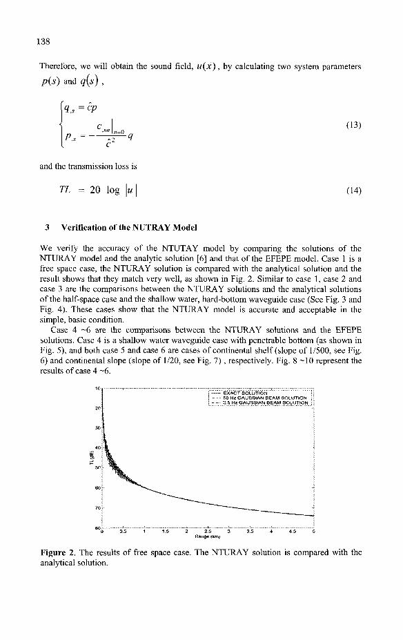
138
Therefore, we will obtain the sound field, u(x), by calculating two system parameters
p(s) and q(s) ,
q,s = CP
'"" \n=0
P,*=—rr^-q
(13)
and the transmission loss is
TL = 20 log \u\ (14)
3 Verification of the NUTRAY Model
We verify the accuracy of the NTUTAY model by comparing the solutions of the NTURAY model and the analytic solution [6] and that of the EFEPE model. Case 1 is a free space case, the NTURAY solution is compared with the analytical solution and the result shows that they match very well, as shown in Fig. 2. Similar to case 1, case 2 and case 3 are the comparisons between the NTURAY solutions and the analytical solutions of the half-space case and the shallow water, hard-bottom waveguide case (See Fig. 3 and Fig. 4). These cases show that the NTURAY model is accurate and acceptable in the simple, basic condition.
Case 4 ~6 are the comparisons between the NTURAY solutions and the EFEPE solutions. Case 4 is a shallow water waveguide case with penetrable bottom (as shown in Fig. 5), and both case 5 and case 6 are cases of continental shelf (slope of 1/500, see Fig. 6) and continental slope (slope of 1/20, see Fig. 7) , respectively. Fig. 8-10 represent the results of case 4 ~6.
— EXACT SOLUTION — SO H i GAUSSIAN SEAM SOLUTION - - 3,5 Hz GAUSSIAN SEAM SOLUTION
Figure 2. The results of free space case. The NTURAY solution is compared with the analytical solution.
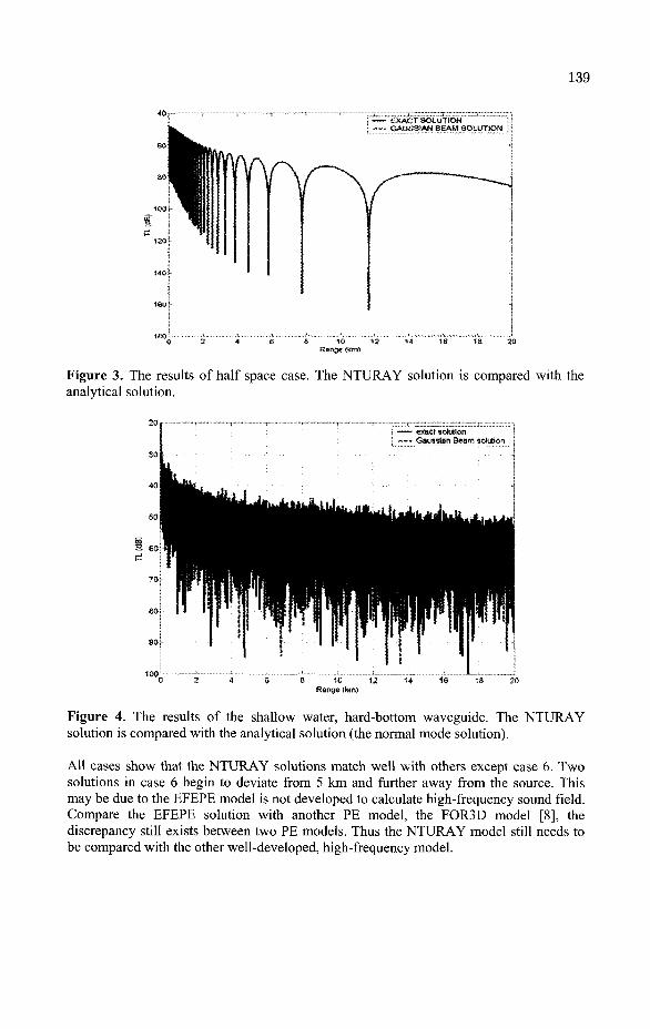
139
EXACT SOLUTION GAUSSIAN BEAU SOLUTION
Figure 3. The results of half space case. The NTURAY solution is compared with the analytical solution.
a 10 12 Range (km)
Figure 4. The results of the shallow water, hard-bottom waveguide. The NTURAY solution is compared with the analytical solution (the normal mode solution).
All cases show that the NTURAY solutions match well with others except case 6. Two solutions in case 6 begin to deviate from 5 km and further away from the source. This may be due to the EFEPE model is not developed to calculate high-frequency sound field. Compare the EFEPE solution with another PE model, the FOR3D model [8], the discrepancy still exists between two PE models. Thus the NTURAY model still needs to be compared with the other well-developed, high-frequency model.

140
Air
100 m Source
10 Km
Receiver
. c=1500 m/s * p=1000kg/m3
Penetrating Bottom c=1550m/s p=1200kg/m3
a = l dB/A
Figure 5. Case 4: the shallow water waveguide with a penetrable bottom.
Receiver
Air
Penetrating Bottom Slope (1/500)
Source c= 1500 m/s , p=1000kg/m3
c=1550m/s ,0=1200 kg/m3
a=\ dB/A Figure 6. Case 5: the case of continental shelf (slope is equal to 1/500) with penetrable bottom.
Air c=1500m/s ,0=1000 kg/m3
c=1550m/s ,0=1200 kg/m3
a =1 dB/A Figure 7. Case 6: the case of continental slope (slope is equal to 1/20) with penetrable bottom.
Penetrating Bottom Slope (1/20)

141
Range <km)
Figure 8. The results of shallow water waveguide with penetrable bottom. The NTURAY solution is compared with the EFEPE solution, and they math quite well.
4 5 6 Range (fan)
Figure 9. The results of continental shelf case (slope is equal to 1/500) with penetrable bottom. The NTURAY solution is compared with the EFEPE solution and match very well.

142
4 5 6 Range (km)
Figure 10. The results of the continental slope case (slope is equal to 1/20) with penetrable bottom. The NTURAY solution is compared with the EFEPE solution; two solutions start to diverge from about 5 km far from the source.
4 Two-layered Bottom Model
According to Frisk [7], the summarized reflection effect of the two layer bottom (as shown in Fig. 11) can be represented by the Rayleigh Reflection Coefficient
R = Ro\ + Rne
\ + R01Rne 2ik,h cos 9 (15)
Air
P o . C o
Half Space
Figure 11. The two layer bottom.
Pl,Cl

The results of the two-layered NTURAY model and the EFEPE model are presented m Fig. 12. It shows that the two-layered NTURAY model is accurate in this case.
• E F E P E solution • G B M 2 solution
1000 2000 3000 4000 5000 6000 7000 8000 9000 10000 Range (m)
Figure 12. The results of the two-layered bottom case. The NTURAY solution is compared with the EFEPE solution.
5 Conclusion
In this paper, the NTURAY model is proposed. The NTURAY is a range-dependent model which uses the Gaussian Beams Method to calculation the high-frequency, long range acoustic field. It can deal with the laterally varying multi-layered ocean environment and calculate the traces and the transmission loss.
Several cases are used to verify the accuracy of the NTURAY, and the results show that the comparisons between analytic solutions or EFEPE solutions and NTURAY solutions are satisfactory.
Reference
1. C. F. Chen, W. S. Hwang, L. W. Hsieh, and Y. T. Lin, "Verification and evaluation of the advanced sonar range prediction system (ASORPS)," National Taiwan University, report of Engineering Science and Ocean Engineering, Underwater Acoustic Laboratory, UAL-NTU TR 0101, 2002.
2. V. Cerveny, M. M. Popov and I. Psencik, "Computation of wave fields in inhomogeneous media - Gaussian beam approach," Geophys. J. astr. Soc. 70, pp.109-128, 1982.
3. V. Cerveny and I. Psencik, "Gaussian beams in two-dimensional elastic inhomogeneous media," Geophys. J. astr. Soc. 72, pp. 417-433, 1983.
4. V. Cerveny and I. Psencik, "Gaussian beams in 2-D laterally varying layered structures," Geophys. J. astr. Soc. 78, pp. 65-91, 1984.

5. M. B. Porter and H. P. Bucker, "Gaussian beam tracing for computing ocean acoustic fields," J. Acoust. Soc. Am. 82(4), pp. 1349-1359, 1987.
6. H. Weinberg and R. Keenan, "Gaussian ray bundles for modeling high-frequency propagation loss under shallow water conditions," J. Acoust. Soc. Am. 100(3), 1996.
7. G. V. Frisk, Ocean and Seabed Acoustics: a theory of wave propagation, Prentice-Hall, NJ, 1994.
8. D. Lee and M. H. Schultz, "Numerical Ocean Acoustic Propagation in Three Dimensions, " Singapore: World Scientific, pp. 138-144, 1995.
A P P L I C A T I O N N I C H E G E N E T I C A L G O R I T H M S T O A V O A I N V E R S I O N
IN O R T H O R H O M B I C M E D I A
MING-HUI LU, HUI-ZHU YANG
Department of Engineering Mechanics, Tsinghua University, Beijing 100084, China
lmh02 @ mails, tsinghua. edu. en
A forward modeling of P-wave propagation in a bi-layer model of an isotropic layer overlying an
orthorhombic layer is performed. The observation data of four differently oriented
common-midpoint (CMP) lines show that P-wave amplitude exhibit strong azimuthal anisotropy. A
formula is deduced to obtain the azimuth angle by using the amplitude variation of four differently
oriented lines. Thomsen anisotropic parameters and the ratio of SV- wave and P-wave vertical
velocity can be inverted from Amplitude Versus Offset and Azimuth (AVOA) by using the Niche
Genetic Algorithms (NGA).The numerical simulation shows that the inversion method has enough
stabilization and precision.
1. Introduction
Seismic detection of subsurface fracture plays an important role in making decisions on drilling locations and determining fluid flow during production1"2. Natural fractures in reservoirs tend to be vertical to the minimum horizontal in-situ stress, so the horizontal transverse isotropy (HTI) model is commonly used to describe a system of parallel vertical penny-shaped cracks embedded in an isotropic host rock. Some scholars have done many researches on fracture prediction by using the properties of azimuthal anisotropy of seismic wave velocities and reflection amplitudes in HTI media, and have obtained some theoretical achievements and oilfield data processing experiences3"7. However, the orthorhombic model (ORT) is believed to be more realistic than HTI model to describe the naturally-fractured reservoirs. The approximate reflection coefficient for a bi-layer model of an isotropic layer overlying an orthorhombic layer has been derived by Corrigan in 1990. In terms of the similar form of the symmetry planes of orthorhombic media and transverse isotropy media, Tsvankin9 introduced Thomsen-style anisotropic parameters10 of transverse isotropy model into P-wave kinematic study on ORT model to deduce a series of simplified velocity formulae. In the same way, Ruger' presented a modified P-wave reflection coefficient formula in ORT media, which is the basis for our study on AVOA inversion. It is known that the inversion algorithm is an important factor to affect the results of inversion. In respect that most of the optimization problems in geophysical prospecting are nonlinear, the conventional Newton's method or gradient method are prone to trapping in local minima. To overcome the problems above, Genetic Algorithm (GA) or simulated annealing algorithm etc. are often applied to nonlinear inversion. As a modified GA, the Niche Genetic Algorithm (NGA) can maintain the population various, meanwhile owns the properties of preventing premature
145

146
convergence11. Therefore, we apply the Niche Genetic Algorithm to the AVOA inversion of fracture parameters in ORT media and obtain a highly precise inversion results.
2. AVOA for ORT Media
The P-wave reflection coefficient for ORT medium has been given by Ruger1 as „ , ^ 1 AZ 1 I Aa 2/3 2 AG
2 Z 2[a a G A^+2(^-)2Ar
a cos^ + A^'sin2 (1)
where i denotes the incidence phase angle, <P is the azimuthal angle defined in this paper as the angle between the [x1;x3] symmetry plane and the first survey line oriented eastward (as shown in Fig.l). Z = pa is P-wave impedance and G = p/32 denotes the SV-wave shear modulus. The average velocity a =l/2(a2 + #,) and the difference Aa = a2-al can be respectively written as functions of the P-wave vertical velocities Of, and CC2 in the upper and lower layer. Corresponding expressions are defined for the shear modulus, the density, and the P-wave impedance. This is similar for Thomsen anisotropy parameters Ae, A S<]), ASa), and Ay, among which Ay relates to the density of fractures linearly7.
line three
line two
line one
ISO
ORT
Fig. 1. Orientation of four survey lines for an isotropic layer overlying an ORT medium.
In a 2-D survey, reflection amplitudes are recorded at different offsets and azimuths
and strong AVOZ is observed in ORT media (shown in Fig.2). Therefore, it is possible to
invert fracture orientation and density from AVOZ information. Generally speaking, the
azimuth angle is unknown ahead of inversion. In this paper, we define the first survey
line oriented eastward as the baseline, then put the second line at the direction of
45degree east-north, and put the third line oriented northward, finally put the fourth line
at the direction of 135degree east-north (shown in Fig.l). When we get the observation
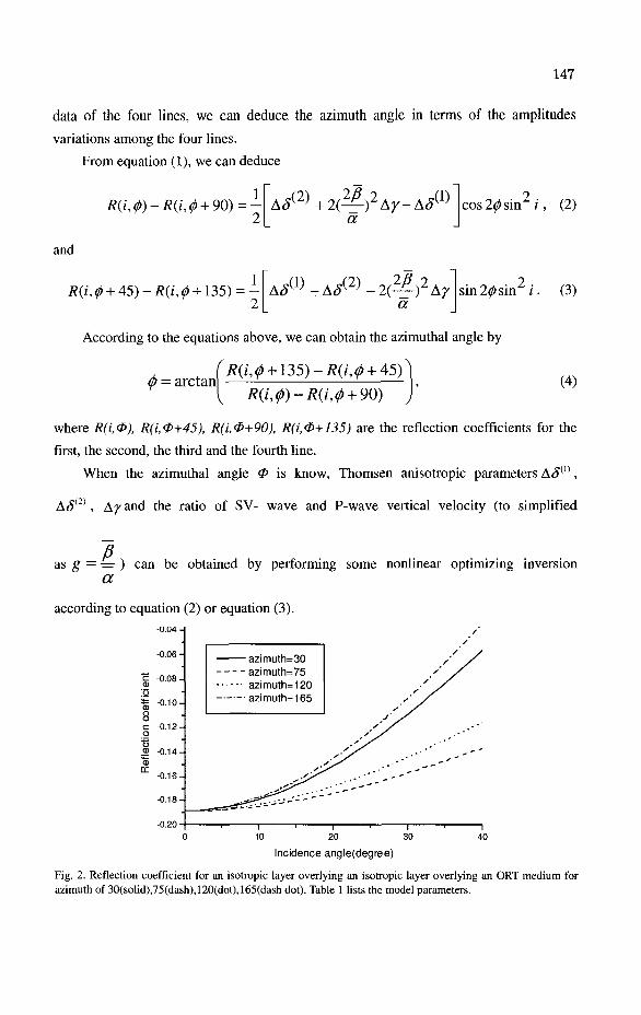
147
data of the four lines, we can deduce the azimuth angle in terms of the amplitudes
variations among the four lines.
From equation (1), we can deduce
R(i, <p) -R(i, </> + 90) = -1
and
R(i,0 +45)- R(i,0 +135) = 1
A8^+2^-)2Ay-AS^ a
AS^-AS^-2(^)2Ay a
cos 20 sin / , (2)
2 sin 2(f) sin / . (3)
According to the equations above, we can obtain the azimuthal angle by
<f> = arctan rR(i,</) +135) -R(i, <fJ + 45)^
V R(i,0)-R(i,0+ 90) (4)
where R(i,&), R(i,&+45), R(i,&+90), R(i,&+135) are the reflection coefficients for the
first, the second, the third and the fourth line.
When the azimuthal angle <£> is know, Thomsen anisotropic parameters A£(1),
AS(2), Ay and the ratio of SV- wave and P-wave vertical velocity (to simplified
P as g = = ) can be obtained by performing some nonlinear optimizing inversion
a according to equation (2) or equation (3).
-U.04 •
-0.06 •
| -0.08-
fc -0.10 • o 8 c -0.12-o t5 jjS -0.14 "S
01 -0.16-
-0.18
-0.20
-azimuth=30 • azimuth=75 azimuth=120
• azimuth=165
o 10 20 30
Incidence angle(degree)
Fig. 2. Reflection coefficient for an isotropic layer overlying an isotropic layer overlying an ORT medium for azimuth of 30(solid),75(dash),120(dot),165(dash dot). Table 1 lists the model parameters.

148
3. NGA Inversion Algorithm
For complex nonlinear optimization problem, the conventional GA is prone to
trapping in local minima owing to its searching the extreme point in a population, which
is also named premature convergence. To overcome the problem above, the population
variety should be maintained during the evolutionary process. In some other words, the
optimum solution and the extreme solution must be co-existed during the search process
to ensure the global optimum solution be obtained by comparing some peaks of every
population.
The NGA is one of the modified algorithms to overcome the problem above, whose
basic idea concludes": the individuals of many populations are relatively independent in
propagation for extending the search space, and the population variety is maintained by
controlling the fitness of the individual. The NGA in this paper combines the benefits of
the distance isolation model and the panmixia model, which are applied to the optimizing
inversion of multi-parameters. The basic idea of the distance isolation model is to divide
a population into many smaller populations (islands), and make the individuals propagate
independently in a small population, and commute individuals among the populations.
The idea of the panmixia model is embodied in the improved standard fitness sharing
method. The sharing function Sh is defined as
Sh(du) Jl-dy/a- dv<a
1 0 other (5)
where a is the given niche radius, dtj is the distance from the individual i and the
individual/ Then the sharing fitness is
f\*i) = n*i)/llshVv)- <6>
In every population, when one individual is close to another one, its sharing fitness
will reduce largely to make it easy to be eliminated, whereas its fitness will decrease
little. Therefore, the rare individuals can be maintained and propagated and the
population variety is preserved very well. This algorithm can prevent premature
convergence and hold the properties of global optimum and fast convergence, especially
for the complex multi-mode optimization problem.
The essence of inversing Thomsen parameters by NGA is an optimization problem
of seeking the adequate model parameters p(ph p2,--pn) to make the theoretical predicted

149
results match with the observation data. The objective function E(p) is defined as
E(p) = j^-fJ[RP(pJ)-K(i)]2
(7)
where Rp(P,i) is the ith predicted amplitude of P-wave, R (i)is the ith observation
data, C is the amplified number, and N is the number of sample.
4. Numerical Simulation
In order to test the effectivity of our inversion method, we perform a numerical
simulation inversion process. First, we substitute the amplitudes calculated in equation
(1) for the observation data required before inversion. The numerical simulation model is
a bi-layer one of an isotropic layer overlying an ORT media. The elastic tensor of ORT
media is as follows (referred to literature 12):
C=
30.779 3.163
3.551
0
0
0
3.163 23.611
2.801
0
0
0
3.551 2.801
22.941
0
0
0
0 0
0
7.903
0
0
0 0
0
0
9.386
0
0 0
0
0
0
10.558
The parameters of velocities and Thomsen parameters in ORT media are calculated
according to the equations in reference [3,9], and the results are listed in Table 1 with the
parameters of the isotropic layer.
Next, substitute the values of these parameters in Equation (1) and obtain four sets
of amplitudes when the azimuthal angle is 30°, 75°, 120°and 165° respectively as
observation data of four survey lines.
Table 1. Parameters of the bi-layer model.
parameter
value
P (kg/m3) a(m/s) /?(m/s) £0) £<2) r fin ISO media
ORT media
2600
2200
4000
3229
2200
1895
0
-0.16
0
-0.026
0
0.168
0
30

150
Second, we substitute four sets of amplitudes in Equation (5), and obtain a curve of
illustrating the relationship between the azimuthal angle and the incidence angle. Fig.3
shows that the azimuthal angle inverted is approximated as 30°and it is highly accurate
compared with the real value.
inc idence angle(d eg ree )
Fig.3. The azimuthal angle inverted.
Third, we use the NGA to invert Thomsen parameters AS, A^and g from the amplitudes difference between line one and line three.
The parameters of NGA are selected as: the population number is 4, the number of individuals in every population is 50, the crossover probability is Pc = 0.8, the mutation probability is Pm- 0.01, the ratio of selection from the parent population is 70%, and the generation number is 30. The ranges of inversion parameters are -0.2 ^ A<r ' S 0, -0.1 ^ AS{2) < 0, 0 < Ay< 0.2, 0.5 <g < 0.8 respectively. The objective function is defined as formula (7) and the amplified number C = l.OE + 6. The inversion results and errors are shown in table 2.
Table 2 Comparison between inversion results and true values.
parameters
real value
inverted value
absolute error
relative error
ASW
-0.16
-0.18
0.02
12.5%
AS(2)
-0.026
-0.027
0.001
3.8%
Ay
0.168
0.164
0.004
2.3%
g
0.566
0.558
0.008
1.4%

151
From table 2, we can conclude that the results of inversion accord well with the real
values of model parameters. The ratio of SV- wave and P-wave vertical velocity inverted
has the smallest error, which can provide a way to estimate SV- wave vertical velocity
accurately because it is difficult to acquire SV- wave vertical velocity directly from the
oilfield observation. The relative error of Ay parameter is only 2.3%, so it is accurate
enough to predict the density of fractures. On Fig.4, we can see that the convergence of
the objective function tends to be stable after the 20th generation, which shows that our
inversion algorithm has fast and stable convergence.
70-
60-
50-
40-
30-
2 0 -
10-
»̂
> \
\
v„„ Generation number
Fig.4 The convergence of objective function
5. Conclusions
In studies of naturally-fractured reservoirs, the orthorhombic model (ORT) is more
realistic than horizontal transverse isotropy (HTI) model. In respect that P-wave
amplitudes are very sensitive to azimuthal seismic anisotropy, the properties of AVOA
can be applied to fracture detection. In this paper, a new method using the amplitudes
variation of four differently oriented common-midpoint (CMP) lines to obtain a highly
accurate azimuth angle is proposed; the procedure of AVOA inversion of Thomsen
anisotropic parameters by using the Niche Genetic Algorithms is described in detail. The
numerical simulation shows that the direction and density of fractures inverted are highly
accurate and the Niche Genetic Algorithms has enough stabilization and precision.
Further study will focus on extending this inversion method to the processing of the
oilfield seismic data.
Acknowledgments
The authors would like to thank the China National Natural Science Foundation for supporting this work under Grant 10272064.

152
References
1. Ruger, A., 1998, Variation of P-wave reflectivity with offset and azimuth in
anisotropic media: Geophysics, 63(3), 935-947.
2. Sayers, CM. and Dean, S., 2001, Azimuth-dependent AVO in reservoirs containing
non-orthogonal fracture sets: Geophysical Prospecting, 49(1), 100-106.
3. Ruger, A., 1997, P-wave reflection coefficients for transversely isotropic models with
vertical and horizontal axis of symmetry: Geophysics, 62(3), 713-722.
4. Perez, M.A., Grechka, V., Michelena, R.J., 1999, Fracture detection in a carbonate
reservoir using a variety of seismic methods: Geophysics, 64(4), 1266-1276.
5. Gray, D. and Head, K., 2000, Fracture detection in Manderson Field: A 3D AVAZ
case history: The Leading Edge, 19(11), 1214-1221.
6. Li, X-Y., Liu, Y-J., and Liu, E. etc., 2003, Fracture detection using land 3D seismic
data from the Yellow River Delta, China: The Leading Edge, 22(7), 680-683.
7. Bakulin, A., Grechka, V., and Tsvinkin, I., 2000, Estimation of fracture parameters
from reflection seismic data-part I, II, and III: Geophysics, 65(6), 1788-1830.
8. Corrigan, D., 1990, The effect of azimuthal anisotropy on the variation of reflectivity
with offset: Workshop on Seismic Anisotropy: Soc. Expl. Geophys. 4IWSA, 1645.
9 Tsvankin, I., 1997, Anisotropic parameters and P-wave velocity for orthorhombic
media: Geophysics, 62(4), 1292-1309
10. Thomsen, L., 1986, Weak elastic anisotropy: Geophysics, 51(10), 1954-1966.
11. Nie, J-X., Yang, D-H. and Yang, H-Z., 2004, Inversion of reservoir parameters based
on the BISQ model in partially saturated porous medium: Chinese J. Geophys. (in
Chinese), 47(6), 1101-1105.
12. Xun, H., 1994, The seismic wave forward and analysis on AVO in anisotropic media:
Ph.D. thesis (in Chinese), Univ. of Petroleum (Beijing), 14.

RECONSTRUCTION OF SEISMIC IMPEDANCE
FROM MARINE SEISMIC DATA
B. R. Mabuza Faculty of Applied and Computer Sciences, Vaal University of Technology,
Private Bag X021, Vanderbijlpark, South Africa
M. Braun and S. A. Sofianos Physics Department, University of South Africa,
P.O. Box 392, Pretoria 0003, South Africa
J. Idier IRCCyN/CNRS, 1 rue de la Noe, BP92101, 44321 Nantes cedex 3, France
(Dated: October 31, 2005)
In this paper we focus our attention on the Marchenko inversion method which requires as input the reflectivity sequence of the medium with the view to reconstructing the seismic impedance from seismic reflection data. The reflectivity sequence and the relevant seismic wavelet are extracted from marine reflection data by applying the statistical estimation procedure known as Markov Chain Monte Carlo method to the problem of blind deconvolution. In order to implement the inversion method, the assumption of pure spike trains that was used previously has been replaced by amplitudes having a narrow bell-shaped form to facilitate the numerical solution of the Marchenko integral equation from which the underlying profile of the medium is obtained. Various aspects of our inversion procedure are discussed. These include questions related to the handling of experimental data and the numerical solution of the Marchenko integral equation using piecewise polynomials.
PACS numbers: 58.11.Ab
I. INTRODUCTION
Various methods for seismic exploration have been employed in the past to extract information on subsurface properties of the Earth. The most commonly applied is the seismic reflection method in which both the source and receiver are spread out on the surface. The success of this method is mainly due to the multi-layered structures of sedimentary basins, which reflect the seismic wavelet back to the surface. In this work we will consider marine exploration only.
In order to obtain quantitative information on subsurface properties, in particular, the seismic impedance, we employ the Marchenko integral equation (MIE) [1-3]. The method is closely connected to the inverse problem [4, 5] and its historical evolution can be found, for example, in Refs. [2, 6, 7]. A complete bibliography of pioneering papers dealing with the inverse problem can also be found in Faddeev's paper [5] and in references therein. As indicated by its name, the inverse scattering problem has a counterpart known as the direct scattering problem, in which one proceeds from the potential to the scattering data. Thus the methodology used for solving the inverse problem relies strongly on the formulation of the direct problem.
For most practical situations in the seismic reflection method, the Ear th can be considered as an elastic medium. The elastic wave equation which can be transformed into a Schrodinger-type equation is therefore adequate for the direct problem. This in turn allows treatment via the Marchenko inverse scattering method.
The solution of the MIE requires as input the reflectivity sequence of the medium which can be
153

154
extracted from the marine reflection data. This can be achieved by applying the Markov Chain Monte Carlo (MCMC) method [8-11] based on the Gibbs sampler to iteratively generate random samples from the joint posterior distribution of the unknowns. The MCMC method is based on Bayesian analysis and provides a general mechanism to sample the parameter vector from its posterior distribution via the Monte Carlo method.
In section II the blind deconvolution approach which uses the MCMC method as an alternative form for simultaneously deconvolving the seismic wavelet and reflectivity sequence from marine reflection data is discussed. In section III the inverse reflection problem and the Marchenko inversion method are briefly described. Calculations and results are given in section IV while the conclusions are summarized in section V.
II. BLIND DECONVOLUTION
A. Deconvolution process
Before discussing the deconvolution process we present a brief description of the convolution model. This model can be described schematically as [12]
measured output = output + noise = wavelet * x + noise,
where x is the reflectivity sequence. Mathematically, it can be written as
min(iV,t)
zt= Yl hkxt.k+1+nt, t = l,...,N + M-l, (1) fc=i
where z is an observed seismic trace of length N + M — 1, h represents the seismic wavelet of length N, x stands for the white reflectivity sequence of the medium of length M and n is a zero-mean white noise of Gaussian type. The noise sequence is characterized by its variance a2 [12]. Eq. (1) can be written in a convolutional form
z = h* x + n . (2)
Our objective is to seperate the reflectivity sequence and seismic wavelet from each other by applying the blind deconvolution procedure.
In the literature the system's unit response is called the reflectivity sequence. In our model it will also include multiple reflections (only a finite number is needed) effected by the system provided the seismic wavelet is shorter than the travel time distance between the consecutive interfaces. For our numerical computations we identify the reflectivity sequence up to a scaling factor with the unit response of the medium B(£), which is discussed in section III.
Deconvolution of the seismic reflection data series z when the source wavelet h is known, is a well-understood problem; however, in some investigations such as ours, only the marine seismic reflection data have been provided and both reflectivity and seismic wavelet should be retrieved from them. In order to estimate these quantities, we apply the blind deconvolution method.
155
We assume the sea floor to consist of several homogeneous layers that are separated by interfaces. Such an assumption makes it possible to express the reflectivity sequence in terms of a Bernoulli-Gaussian (BG) sequence [13, 14]. Thus, the reflectivity sequence that defines the generalized BG sequence can be modeled by using two random sequences expressed as [12]
Xk = rkQk , (3)
where r = (rk) denotes a zero-mean Gaussian white sequence with variance of and q = (qk) stands for the Bernoulli sequence with the probability parameter A being equal to its mean value [15]. For the probabilities associated with this sequence we have
P(9fc = l ) = A, (4)
P(qk = 0) = l - \ , (5)
tha t is, the random variable qk is one with probability A and zero with probability 1 — A. The probability of the whole sequence q reads
P(qW = Y[P(qk) = \n(i-x)M-n, (6) k
where n is the number of ones in the sequence.
B. Markov Chain Monte Carlo method
We are concerned with the MCMC method in a pure Bayesian approach. Upon using the Bayes' rule, we can write the probability distribution in the form [16]
Pm=^m, (7) where 9 stands for all parameters of the problem [17], tha t is,
8 = (h,x,\,a2), (8)
and h, x, A, and a2 have the same meaning as above. P(9\z) is the posterior probability of the model conditional on the observed da ta z, P(0), and P(z) describe the prior knowledge and seismic reflection data respectively while P(z\0) describes the discrepancy between the model and observation.
The complete joint probability distribution is expressed in the form [16]
P(8\z) oc P(z\0)P(0), (9)
since P(z) is in this case a normalizing constant. The MCMC algorithm is iterative and may require a number of iterations before the first sample from the correct distribution can be provided. These initial iterations are called burn-in iterations and should not be used in the statistical analysis. Thus, the estimation of reflectivity sequence and the seismic wavelet is determined by the simulation of random variables via the MCMC algorithms based on the Gibbs sampler [9], which is regarded

156
as the best known and most popular of the MCMC algorithms [10]. It is an algorithm in which the vector Q(k+l) is obtained from 0^ by updating the vector elements one at a time. The prior distribution in Eq. (9) can be written as
P(0) = P(x\X)P(X)P(h)P(a2), (10)
where P(h) = P(<r2) = P(X) = 1 are flat prior probability densities and P(x\X) is described by a Bernoulli-Gaussian distribution. Upon using Eq. (10), we can write Eq. (7) in the form
pm_P(z\«2,x,X)P(x\X)P(h) ^
The assumption of a white Gaussian noise sequence n of variance a2 leads to
P(z\a2,x,X) = (2-Ka2)^N+M-1^2 exp
h * •
2a2 (12)
For our purpose, we need to calculate the distributions P(h\z,x,a2, A), P(x\z,h, X,a2), P(a2\z,x,h,X), and P(X\z,x, h,a2). Thus, Eq. (11) can be employed to handle the relevant re-sampling processes.
1. Re-sampling of the amplitude of the reflectivity sequence
The reflectivity sequence x contains information about the Earth 's structure. In order to statistically separate it from the seismic wavelet we use the BG white sequence model [13]: P(x)=nmP(*m), With
P(xm) - (1 - X)5(xm = 0) + AJV(0, B2), (13)
where M is a Gaussian distribution with specified mean and variance and where A € (0,1) is the probability that xm = 1, and both A and g2 are unknown. It can be shown [13] that the posterior probabilities involving single components of the vector x remain Gaussian mixtures with a structure comparable to that of Eq. (13). More precisely,
where X-
P(xm\X,h,z,x^m,) ~ (1 - Xm)S{xv
( i i , . . . , i m - i , i m + i , . . . , X M ) a n d
0) + XmU(x*m,al
a V o-2 + e2\\h\\2
fih'en),
1 + l - A Q V2 C Tm
and
-h*x{m) ,
(14)
(15)
(16)
(17)
(18)
where x<m> is identical to x except for Xm = 0. Using Eqs. (14)-(17), the components xm of the reflectivity sequence can be re-sampled, one at a time.
157
2. Resampling of the seismic wavelet
In order to re-sample the seismic wavelet h, we deduce from the Bayes rule that P(h\a2,x,z) oc P(z\a2,x,h), given P(h) = 1, where P(z\a2,x, h) is given by Eq. (12). Moreover, it is easy to check the following identity:
_\\z~h*xf =_^{h_ii)TR_l{h_^ (19)
where
» = {XTX)-1XTz, (20)
and
R = (XTX)-1a2l, (21)
where X is the Toeplitz matrix of size (N + M — 1, N) such that
Xh = h*x. (22)
This allows us to conclude that the posterior probability of h is a multivariate Gaussian with mean vector n and with covariance matrix R. The latter probability is easy to sample according to h = fi + Qe, where e is a normalized Gaussian white noise and QT is a square root matrix of R (that is, such that R = QQT), such as the one resulting from the Cholesky decomposition.
3. Re-sampling of the hyperparameter a
Given P(<J2) = 1, it is also true that P(a2\z,x, h, A) ex P{z\a2,x, h). As a function of a 2 , Eq. (12) takes the form
P(z\a2,x,\) = p j S T T e x p ( - / 3 / a 2 )
up to a multiplicative constant, with a = (N + M — l ) / 2 — 1 and f3 = \\z — h * x\\2/2, which means that the posterior probability of a2 follows an inverse gamma distribution of parameters (a, /3). The latter can be easily sampled by taking the inverse of a gamma random generator output with the same parameters.
4- Re-sampling of the hyperparameter A
The reflectivity sequence x gathers all the information about A contained in (z,x,h, a2), tha t is, P(X\z,x,h,a2) = P(\\x). Following [13], let us remark that the Bernoulli sequence q can be retrieved from x with probability one according to q^ = 1 if Xt ^ 0, q^ = 0 otherwise. Thus, P(\\x) = P(X\q), the latter being proportional to P(q\X) since we assumed a flat prior P(A) = 1. Finally, according to Eq. (6), we get
P ( A | z , x , / i , a 2 ) c x A n ( l - A ) M - n , (23)
which belongs to the family of beta probability densities B(a,f3) with a = n+1 and (3 = M — n + 1.

158
III. INVERSE REFLECTION PROBLEM
The one-dimensional seismic wave equation for the elastic displacement u is given by [18]
d2u d ( 2du pW-dz{pC8-z)=°' W
where t is the time, z is the space coordinate along the direction of propagation, p = p{z) is the density of the medium, and c = c(z) is the speed of the seismic wave. We are considering here a longitudinal displacement in the ^-direction. The Marchenko integral equation is directly applicable to the case of inversion with a seismic wave normally incident on a planar stratified medium, provided tha t the one-dimensional seismic wave equation is converted to the Schrodinger equation. Thus, the coordinate variable z is changed to the travel time £ defined by
dz= c^y • (25)
When integrating Eq. (25) we obtain
*=La£)"' (26)
which is the travel time for a pulse to move from the origin to position z. Upon using this relation we can rewrite the wave equation as
, ,d2u d ( ,^du\ , s
" « > < * = a e ( " « > a e ) ' (27)
where r/(£) = pc is the seismic impedance of the medium. Defining rf> via ip = yjiju we obtain
d2ip d2i> T ,
where V is given by
For an ansatz of the form il>(£,t) = exp(—ikt)f(£) the Schrodinger-type equation
nO = - ^ r - (29)
~ + (k2-V(O)f = 0, (30)
is obtained. From the definition of V in Eq. (29) we can write
d2^j
di2 V(OVV = 0, (31)
which is a reduced form of Eq. (30) with k = 0. For the inversion procedure we apply the Marchenko integral equation given as [2]
K{£,t) + B{£ + t)+ dt'K(Z,t')B(t + t')=0, |t| < f , (32)

159
for which K(£,t) = 0, for \t\ > £, and it denotes a non-causal function while the function B is causal and represents a reflectivity sequence. The function K satisfies the wave equation given by Eq. (28). Thus,
K(C,-O = 0, (33)
and
V ( 6 = 2 ^ . (34) at.
The output kernel K(£,£,') can be determined by using the collocation method and piecewise polynomials, in our case Hermite splines. The Schrodinger-type equation, Eq. (30), is equivalent to the Marchenko integral equation via Eq. (34). The seismic impedance r\ can be calculated from the potential V(£) in Eq. (29) or directly from the relation [19]
v(0 = v(o) ( 1 + / + *K.£ 'K') • (35)
This means that , given the ??(0), the seismic impedance rj(£) for £ > 0 can be recovered from the knowledge of the kernel K(£,t).
IV. RESULTS
We illustrate the use of the blind deconvolution method on recorded marine seismic reflection da ta derived from a seismic survey in a deep water location in the North sea. We use data collected with a streamer containing 240 hydrophone groups. The group interval is 15 m. The sampling rate is 4 ms and the total length is 8 s. Each trace is composed of 2001 samples as shown in Figs. 1 and 2. Depicted in Fig. 3 are the seismic reflection data. We migrated the seismic reflection data using the standard moveout correction method [20] (or any other standard textbook) with the result as shown in Fig. 4.
The main modification as compared to Chen's version [13] is tha t we assume a shape given by
s = [0.1, 0.4, 1.0, 0.4, 0.1], (36)
instead of pure spikes in order to have a narrow bell-shaped form to facilitate the numerical solution of the Marchenko inversion. This means that the observation model, Eq. (2), now becomes
z = h*s*x + n, (37)
where s is a known shape. If the shape s is equal to unity then of course the original equation (2) is recovered. We use in our calculations the seismic dataset from Fig. 4 which only include seismic traces from groups 90 to 240 since the normal moveout correction method did not give satisfactory results for the other groups because their offsets are too large. In addition we used all migrated traces collectively as observed seismic reflection da ta and modified the MCMC algorithm accordingly.
We also note, tha t the observed seismic reflection da ta are not calibrated, that is, they only provide relative amplitudes. The details of the source of the signal, tha t is, the airgun, are also

160
not known. Therefore, the reflectivity sequence that we obtain from the statistical procedure will be related to the unit response of the medium by a suitable factor. This calibration problem can be solved by using additional information, such as the seismic impedance jump at the ocean bottom if known via other means.
For our purpose we model the sea floor as fluid so that only the compressional seismic wave can be supported. If we assume that the sea bot tom consists of silt (fine sand or soil) and that the density changes much more than the velocity, then we can write [21-23]
— = 1.7, (38) P\
where pi = 1000 kg m - 3 is the density of the sea water and P2 = 1700 kg m~ is the density of silt. Similarly, if we assume that the velocity of sound does not change much, then we obtain the ratio
— = 1.05, (39) c\
where c\ = 1500 m s - 1 is the velocity of the seismic compressional wave in sea water and c-2 = 1575 m s - 1 is the velocity of the seismic compressional wave in silt. Thus, the seismic impedance is expressed in the form
Z » = £22* = 1 . 7 8 5 , (40) Vi PiCi
where rji is the seismic impedance of the sea water and r]2 is the seismic impedance of silt. Assuming this value of the ratio 772/V1 w e proceed to re-scale the amplitude of the estimated reflectivity sequence by a suitable factor. This factor is obtained by scaling the amplitude of the input kernel into the Marchenko equation, such that the inversion procedure yields a first jump approximately equal to r\il"t)\ = 1.785.
Shown in Fig. 5 is the seismic wavelet extracted from the migrated seismic reflection data in Fig. 4. Fig. 6 depicts the statistically retrieved reflection sequence corresponding to the seismic wavelet in Fig. 5. The estimated seismic impedance is shown in Fig. 7. Fig. 8 shows the reflectivity sequence scaled by a suitable factor and the corresponding estimated seismic impedance is shown in Fig. 9, while in Fig. 10 we observe the invariance of peak ranking and location of peaks between the estimated seismic impedances with and without a scaling factor. Thus a lot of information can be retrieved even without knowledge of the proper scaling factor.
V. CONCLUSIONS
We have presented the blind deconvolution of the Marine seismic reflection data wherein the Bernoulli-Gaussian white sequence model for the reflectivity sequence has been used. We presented an MCMC method for simultaneously estimating seismic wavelet and reflectivity sequence under the Bayesian approach. With the estimated reflectivity sequence at hand, the seismic impedance of the Ear th medium has been reliably estimated by applying the Marchenko inverse scattering method.
However, since the marine seismic reflection data are not calibrated and the details of the source signal are not known, we related the acquired reflectivity sequence to the unit response of the

161
Ear th medium by a suitable scaling factor.
Since the statistically acquired reflectivity sequence and seismic wavelet appear geophysically reasonable, the blind deconvolution of reflection data is judged as successful. The results we have obtained indicate that we have uncovered the information about the seismic impedances that are coded into the measured seismic traces.
Further work is under way to handle data from other seismic surveys.
ACKNOWLEDGEMENTS
I would like to place on record my appreciation to Mr George Smith of the Department of Geochemistry at the University of Cape Town for his enlightening discussions and support for this research by generously giving me access to seismic reflection data from a deep water location in the North Sea which was used to test the model in this thesis.
40
30
20
•§ io
•a. o s * -10
-20
-30
-40
1 1 1 1
-i i i i
1 1 1 marine data —
l , 1 1
i i i
--~
----
FIG. 1: 90th seismic trace
150
100
50
0
-50
-100
—^M/Vv~—4
marine data -
I I«4*I* , >* ' I I | I>* '1 1 ' ' * '
FIG. 2: 240th seismic trace.

162
E-i
0 T
3 -
4 -
5 -
6 -
7 -
0 50 100 150
Number of traces
FIG. 3: The seismic data without moveout correction.
0
-1 +
-2
-3
-4
-5
-6
-7
w<VW •^••wrifei^iv^g^-Ajasa
90
.- c .^ipvv. ::.-MU,
1—
120 — i —
150 180
number of traces
210 240
FIG. 4: The seismic data with moveout correction.
[1] Z. S. Agranovich and V. A. Marchenko The Inverse Problem of Scattering Theory. New York: Gordon and Breach, 1963
[2] K. Chadan and P.C. Sabatier, in Inverse Problems in Quantum Scattering Theory, 2nd edition, Springer, Berlin, Heidelberg, N.Y (1982 and 1989).
[3] D. N. Gosh Roy, in Methods of inverse problems of scattering Theory, Gordon and Beach N.Y (1963) p.2, 4; D. N. Gosh Roy, in Methods of inverse problems in Physics, CRC Press, Boston, (1991).
[4] I. Kay, The inverse Scattering Problem. New York: University Research Report, EM-74, 1955. [5] L.D. Faddeev, Uspekhi Matem. Nauk 14, II, 57; English translation: J. Math. Phys. 4, 72 (1963). [6] D. L. Colton and R. Kress, Inverse Acoustic and Electromagnetic Scattering Theory. Berlin: Springer-
Verlag, 1992.

163
0.2
FIG. 5: Seismic wavelet statistically estimated from a dataset in Fig. 4.
Reflectivity _
4 j ^ f
J L 0 0.5 1 1.5 2 2.5 3 3.5
t
FIG. 6: Statistically estimated reflectivity sequence corresponding to a seismic wavelet in Fig. 5.
[7] A. G. Raima, Multidimensional Inverse Scattering Problems, Longman Scientific and Wiley, New York, 1992.
[8] C. Andrieu, N. D. Freitas, A. Doucet and M. I. Gordan, An introduction to MCMC for machine learning Mach. Learning, 50, 2003, p. 5-43.
[9] C. P. Robert, The Bayesian choice, New York: Springer-Verlag, 1994. [10] A. Buland and H. Omre, Bayesian wavelet estimation from seismic and well data, Geophysics, Vol.
No. 6, November-December 2003, p. 2000-2009. [11] S. Geman and D. Geman, Stochastic relaxation, Gibbs distribution and the Bayesian restoration of
images, IEEE Trans. Pattern. Anal. Mach. Intell., vol. 6 1984, p721-741. [12] J. M. Mendel, Maximum-Likelihood deconvolution: A journey into model-based signal processing,
Berlin, Germany: Springer-Verlag, New York, Berlin, 1990, p. 4-15. [13] Q. Cheng, R. Chen, and T. -H. Li, Simultaneous wavelet estimation and deconvolution of reflection
seismic signals, IEEE Trans. Geosci. and Remote sensing, vol. 34, no. 2, March 1996, p. 377-384 [14] J. Kormylo and J. M. Mendel, Maximum-likelihood detection and estimation of Bernoulli-Gaussian
processes, IEEE Trans. Inform. Theory, vol. IT-28, p.482-488, 1982. [15] A. Papoulis, Probability, random variables and stochastic processes. McGraw-Hill, New York, 1965
and 1984. [16] J. Wang and N. Zabaras, Hierarchical Bayesian models for inverse problems in heat conduction, Inverse
Problems 21, 2005, p. 183-206. [17] S. V. Vaseghi, Advanced signal processing and digital noise reduction, John Wiley and Teubner,
Chichester, New York, 1996 p. 66-67, 71-72. [18] R. Burridge, in Wave motion 2, North-Holland Publishing Company, 1980, p. 305-323.
amp
litu
de
rela
tive
4
2
0
-2
-4
-
1 1 1
IIIIJLUJUA wTTPTnr
Iff

164
1.14
1.12
a, 1.1
S 1.08
& 1.06
Z 1-04
| 1.02 "o3
0.98
0.96
1
1
- 1
1 1 1 1 1 1 1 impedance! —
1 \ i
[Vi « • u i r - p, v
1 1 1 1 1 1 1 1
_ -----
0 0.2 0.4 0.6 0.8 1 1.2 1.4 1.6 1.8
?
FIG. 7: Estimated seismic impedance corresponding to a statistically estimated reflectivity sequence in Fie. 6.
~
-
Reflectivity
U ' U u h * J 1>JL >">' IWKV'fl (( f p ,
i i i i l l i
r: I - 1 0
-20
0 0.5 1 1.5 2 2.5 3 3.5
FIG. 8: Scaled reflectivity sequence in Fig. 6.
[19] W. C. Chew, in Waves and fields in inhomogeneous media, Van Nostrand, Reinhold, New York, 1990, p.49-52, 532-547.
[20] J. M. Reynolds, in An introduction to Applied and Environmental Geophysics, John Wiley and Sons, Singapore, 1997, p. 218, 226, 233, 360.
[21] F. B. Jensen, W. A. Kuperman, M. B. Porter, H. Schmidt, in Computational ocean acoustics, American Institute of Physics, New York, 1994, p. 41-54.
[22] E. L, Hamilton, Geoacoustic modeling of the sea flour, J. Acoust. Soc. Am. Vol. 68, 1980, p. 1313-1340. [23] E. L. Hamilton, Acoustic properties of sediments, in Acoustics and Ocean Bottom, edited by A. Lara-
Saenz, C. Ranz-Guerra and C. Carbio-Fite (C.S.I.C, Madrid, Spain, 1987), p. 3-58.

165
FIG. 9: Estimated seismic impedance corresponding to the scaled reflectivity sequence in Fig. 8.
FIG. 10: Comparison between the estimated seismic impedances in Figs. (9) and (7) with and without a scaling factor respectively.


Journal of Computational Acoustics © IMACS
C H A R A C T E R I Z A T I O N OF A N U N D E R W A T E R A C O U S T I C SIGNAL U S I N G T H E STATISTICS OF T H E WAVELET S U B B A N D C O E F F I C I E N T S
MICHAEL I. TAROTJDAKIS
Department of Mathematics, University of Crete, Institute of Applied and Computational Mathematics, FORTH,
P.O.Box 1385, 711 10 Heraklion, Crete, Greece taroud@iacm. forth, gr
GEORGE TZAGKARAKIS and PANAGIOTIS TSAKALIDES
Department of Computer Science, University of Crete, Institute of Computer Science, FORTH,
P.O.Box 1385, 711 10 Heraklion, Crete, Greece {gtzag, tsakalid} @ics. forth.gr
A novel statistical scheme for the characterization of underwater acoustic signals is tested in a shallow water environment for the classification of the bottom properties. The scheme is using the statistics of the 1-D wavelet coefficients of the transformed signal. For geoacoustic inversions based on optimization procedures, an appropriate norm is defined, based on the Kullback-Leibler divergence (KLD), expressing the difference between two statistical distributions. Thus the similarity of two environments is determined by means of an appropriate norm expressing the difference between two acoustical signals. The performance of the proposed inversion method is studied using synthetic acoustic signals generated in a shallow water environment over a fluid bottom.
1. Introduction
Recently, a new method for the classification of the underwater acoustic signals has been proposed by the authors, aiming at the definition of an alternative set of "observables" to be used for geoacoustic inversions l. The study was motivated by the fact that it is not always possible to obtain a set of identifiable and measurable properties of the acoustic signal to be used in the framework of an inversion process. As the efficiency of an inversion procedure is directly related to the character of the observables, a major task on a specific physical problem is to define observables which will be more sensitive to changes of the environmental parameters and easily identified in noisy conditions. In previous works *'2 it was shown that the modelling of the statistics of the wavelet subband coefficients of the measured signal, provides an alternative way for obtaining a set of observables which is easily calculated and has the necessary sensitivity in changes of the environmental parameters, so that its use for inversions to be well justified. Here, this method is tested in shallow water environments for the recovery of the bottom parameters. The inversion is based on an optimization scheme utilizing the Kullback-Leibler divergence to measure the similarity between the observed signal and a signal calculated using a candidate set of bottom parameters.
167

168
2. The classification scheme
In the framework of the proposed approach, an acoustic signal is classified using the statistics of the subband coefficients of its 1-D wavelet transform. In particular, the measured signal is decomposed into several scales by employing a multilevel 1-D Discrete Wavelet Transform (DWT) 3. This transform works as follows: starting from the given signal s(t), two sets of coefficients are computed at the first level of decomposition, (i) approximation coefficients Al and (ii) detail coefficients Dl . These vectors are obtained by convolving s(t) with a low-pass filter for approximation and with a high-pass filter for detail, followed by dyadic decimation. At the second level of decomposition, the vector Al of the approximation coefficients, is decomposed in two sets of coefficients using the same approach replacing s(t) by Al and producing A2 and D2. This procedure continues in the same way, namely at the k-th level of decomposition we filter the vector of the approximation coefficients computed at the (k-l)-th level.
2.1. Derivation of the statistics of the wavelet subband coefficients
The Feature Extraction (FE) step is motivated by previous works on image processing 4 '5,6. The signal is first decomposed into several scales by employing a 1-D DWT as described above. The next step is based on the accurate modelling of the tails of the marginal distribution of the wavelet coefficients at each subband by adaptively varying the parameters of a suitable density function. The extracted features of each subband are the estimated parameters of the corresponding model. For the acoustical signals studied, the wavelet subband coefficients are modelled as symmetric alpha-Stable (SaS) random variables.
The SaS distribution is best defined by its characteristic function 7 '8:
( K w ) = e x p ( ? < 5 w - 7 a M a ) , (!)
where a is the characteristic exponent, taking values 0 < a < 2, 5 (—oo < S < oo) is the location parameter, and 7 (7 > 0) is the dispersion of the distribution. The characteristic exponent is a shape parameter, which controls the "thickness" of the tails of the density function. The smaller the value of a, the heavier the tails of the SaS density function. The dispersion parameter determines the spread of the distribution around its location parameter, similar to the variance of the Gaussian.
In general, no closed-form expressions exist for the SaS density functions. Two important special cases of SaS densities with closed-form expressions are the Gaussian (a = 2) and the Cauchy (a = 1). Unlike the Gaussian density, which has exponential tails, stable densities have tails following an algebraic rate of decay (P(X > x) ~ Cx~a, as x —> 00, where C is a constant depending on the model parameters), hence random variables following SaS distributions with small a values are highly impulsive.
2.2. Feature Extraction
After the implementation of the 1-D wavelet transform, the marginal statistics of the coefficients at each decomposition level are modelled via a SaS distribution. Then, to extract

169
the features, we simply estimate the (a, 7) pairs at each subband. Thus, a given acoustic signal S, decomposed in L levels, is associated with the set of the
L + l pairs of the estimated parameters:
S ^ {(a i , 71), (a2, 72), • • •, («L+i, 7 i+ i )} . (2)
where (o^, 7$) are the estimated model parameters of the i-th subband. Note that we follow the convention that i = 1 corresponds to the detail subband at the first decomposition level, while i = L + 1 corresponds to the approximation subband at the L-th level. The total size of the above set equals 2(_L + 1) which means that the content of an acoustic signal can be represented by only a few parameters, in contrast with the large number of the transform coefficients.
As it has already been mentioned, the FE step becomes an estimator of the model parameters. The desired estimator in our case is the maximum likelihood (ML) estimator. The estimation of the SaS model parameters is performed using the consistent ML method described by Nolan 9, which provides estimates with the most tight confidence intervals.
2.3. Similarity Measurement
In the proposed classification scheme, the similarity measurement between two distinct acoustic signals was carried out by employing the Kullback-Leibler divergence (KLD) 10. As there is no closed-form expression for the KLD between two general SaS densities which are not Cauchy or Gaussian, numerical methods should be employed for the computation of the KLD between two numerically approximated SaS densities.
In order to avoid the increased computational complexity of a numerical scheme, we first transform the corresponding characteristic functions into valid probability density functions and then the KLD is applied on these normalized versions of the characteristic functions. Due to the one-to-one correspondence between a SaS density and its associated characteristic function, it is expected that the KLD between normalized characteristic functions will be a good similarity measure between the acoustic signals.
If 4>{UJ) is a characteristic function corresponding to a SaS distribution, then the function
fa) = ^ (3) is a valid density function when
/
oo 4>(u>) duo.
-00
For the parameterization of the SaS characteristic function given by Eq. (1) and assuming that the densities are centered at zero, that is 5 = 0, which is true in the case of wavelet subband coefficients since the average value of a wavelet is zero, the normalization factor is given by

170
By employing the KLD between a pair of normalized SaS characteristic functions, the following closed form expression is obtained 4:
^ll^) = ln(^)-^+(jr.^l (5) \CXJ « i V71/ r ( —)
where (on, %) are the estimated parameters of the characteristic function <j>i(-) and C; is its normalizing factor. It can be shown that D is the appropriate cost function for our application as DfyiWfa) > 0 with equality if and only if (on, 71) = («2> 72)-
Thus, the implementation of an L-level DWT on each underwater acoustic signal results in its representation by L + 1 subbands, (D\, D2, • • •, DL,AL), where Di, A{ denote the i-th level detail and approximation subband coefficients, respectively. Assuming that the wavelet coefficients belonging to different subbands are independent, Eq. (5) yields the following expression for the overall distance between two acoustic signals Si, S2:
L+l
£(S1||S2) = ^£(<k,fcll<k,fc)- (6) fc=i
3. Study of the sensitivity of the K L D for geoacoustic inversions
In order to validate the proposed classification scheme, first we need to study the sensitivity of the proposed cost function, which measures the similarity with respect to changes of the environmental parameters. Our previous efforts in this respect were mainly oriented towards the sensitivity of the KLD with respect to small changes of the sound speed profile in the water column. First we observed that the set of statistical parameters of the subband coefficients of a specific signal, propagated through the water column, change significantly when the sound speed profile varies and eventually that the KLD is a suitable tool for monitoring the corresponding model parameters' variation 1 . In the last paper, we have also shown that similar conclusions can be derived for the sensitivity of the KLD when applied to signals measured after interacting with different types of ocean beds. The classification parameters of the sea-bed are typically the compressional and shear velocities, the densities of the various layers, the attenuation coefficients and the thickness of the sedimentary layers. In order to simplify the study we had chosen to simulate experiments by assuming semi-infinite fluid bottoms, thus restricting our environmental parameters to compressional velocity and bottom density only.
Here, we extend this study by adding the case of an ocean bottom consisting of two layers of fluid material. The properties of the substrate are considered constant, while we allow the compressional velocity and density of the sedimentary layer to vary within prescribed limits. We simulate the propagation of an acoustic pulse of central frequency /o = 200 Hz and bandwidth A / = 50 Hz over a distance of R = 5 km and we apply the proposed classification scheme to the simulated measurements for a source and receiver pair placed at mid-depth of the water column. The environmental parameters for the reference environment

171
appear in Table I. We estimated the statistics of the four subband coefficients of the 3-level 1-D wavelet transform applied to each one of the synthetic signals and the KLD between a reference signal and the set of simulated signals that are obtained by changing the sediment compressional velocity from the value of c& = 1550 m/sec to the value of Cj, = 1650 m/sec in steps of 5 m/sec and the density from pi, = 1180 kg/m3 to p& = 1220 kg/m3 in steps of 1 kg/m3. We have chosen to restrict our analysis to narrow limits of the two parameters in order to focus on small variations of the geoacoustic parameters. It should also be pointed out that we have chosen to study a two layered bottom in order to assess the performance of the KLD in cases where a small part of the bottom changes.
Table 1. The shallow water environment.
Water Depth (H) Range (R) Central Frequency (/o) Bandwidth ( A / ) Source/Receiver depth
Sound speed profile in the water: cw{0) cw(50) cw{200) Sediment layer :
Cb
Pb
Semi-infinite substrate:
Csb
Psb
200 m 5 km
200 Hz 50 Hz 100 m
1500 m/sec 1490 m/sec 1515 m/sec
1550 m/sec 1200 kg/m3
1800 m/sec 1500 kg/m3
The simulated data are calculated using the Normal-Mode program MODE1 developed at FO.R.T.H. These data are provided as input to the inverse discrete Fourier transform to yield the signals in the time domain.
Each of the time-domain signals is decomposed by implementing a 3-level 1-D DWT using the db2 and db4 wavelets. The reference signal is that corresponding to the reference environment.
Fig. 1 displays the KLD between the reference signal and each signal corresponding to the geoacoustic parameters indicated at the axes of the diagram. In order to be consistent with previous studies, we have included two plots in the figure, the first of which corresponds to the case where both the approximation and detail subbands are considered and the second corresponding to the case where only the detail subbands are taken into account. The star in the two plots corresponds to zero KLD, that is, its coordinates are equal to the geoacoustic parameters of the reference signal.
It can be seen that the inclusion of the approximation subband only affects the discrim-

172
db2 , APPROX. + DETAILS
301 ' 1 ' • > • > J 1191 1192 1193 1194 1195 1196 1197 1196 1199
P,b [kg/m3] db2 , DETAILS
p^IkgAn3]
Fig. 1. KLD between the reference signal and signals corresponding to different values of the sediment compressional velocity and density, decomposed with the db2 wavelet, using (a) all wavelet subbands and (b) only the details
db4 , APPROX. + DETAILS
8 0 i 1 , 1 1 1 1 1 uJ
1191 1192 1193 1194 1195 1196 1197 1198 1199
Psb [kg/m3] db4 , DETAILS
Fig. 2. KLD between the reference signal and signals corresponding to different values of the sediment compressional velocity and density, decomposed with the db4 wavelet, using (a) all wavelet subbands and (b) only the details
ination power of the KLD between the reference signal and the signals which are already "far" from it.
Fig. 2 presents the KLD between the reference signal and each signal corresponding to different geoacoustic parameters when all the signals are decomposed using the db4 wavelet. As we can see, there is an improvement in comparison with the results provided by the db2 wavelet, which is a good indication that the db4 wavelet can be used with confidence for performing the proposed classification process.
Fig. 3 presents the variation of the KLD between a reference signal corresponding to a

173
0.012
0.01
0.008
Q
-J 0.006
0.004
0.002
1"180 1185 1190 1195 1200 1205 1210 1215 1220
Psb[kg/m3]
Fig. 3. KLD between each one of the signals corresponding to the specific densities of the sediment layer and signals corresponding to different values of the sediment density, decomposed with the db4 wavelet.
sediment density other than that of the reference environment and the signals corresponding to sediment layers of different densities within the limits adopted in the previous study. The compressional velocity is considered constant (=1600 m/sec) for each one of these signals. The purpose of the study illustrated in Fig. 3 is to assess the performance of the classification scheme for small variations of the bottom parameter which is known to be the less accurately estimated by any inversion scheme applied to acoustical data, namely the bottom density, for a class of different reference values. Although the reference values are chosen within the prescribed limits, they can be used for the derivation of more general conclusions with respect to the performance of the proposed classification scheme. We observe that, for each one of the reference signals, the correct value of the bottom density is obtained with confidence limits that are narrow enough to ensure a reliable estimation of the parameter. This observation is again consistent with that of the preliminary studies presented in l .
4. Conclus ions
The purpose of the present paper was to provide additional evidence of the reliability and good behavior of an acoustic signal classification scheme based on a SaS modelling of the coefficients of a 1-D wavelet decomposition. The scheme was originally developed for the classification of the acoustical signals to be used for tomographic applications and has illustrated its efficiency through simulations corresponding to shallow water environments. At the present stage, it is the performance of the KLD, being used so far for signal similarity measurements, which is systematically studied. This is considered to be the first necessary step before proceeding to the inversions. Here, the sensitivity of the KLD with respect to variations of the sediment parameters is studied as an additional step towards the full validation of the proposed method as the basic tool for geoacoustic inversions. The results presented here, based on simulated signals in shallow water environments over a
\
\
1186 -*-• 1192
1199
1205 1212 1220
'• y
y/ \ j-^*-
, ,,«_. -'<;.., _,

174
two-layered b o t t o m , s u p p o r t our s t a t emen t t h a t t h e proposed technique can classify, w i th
high probabil i ty, an unde rwa te r signal in t h e correct envi ronment where it was recorded. I t
is also i m p o r t a n t t o no te t h a t conclusions derived in previous s tudies wi th respect t o t h e
use of specific wavelets or t he use of specific s u b b a n d s are also derived here, which is an
addi t iona l indicat ion t h a t t h e p roposed classification scheme is robus t in i ts behavior .
T h e next s t ep in our s t u d y is t h e appl icat ion of t h e signal classification scheme to ac tua l
inversion procedures involving mul t id imensional search spaces and , if possible, t o acoustical
signals from real exper iments .
R e f e r e n c e s
1. M.I.Taroudakis, G. Tzagkarakis and P. Tsakalides, "Classification of shallow-water acoustic signals via alpha-Stable modeling of the 1-D wavelet coefficients," to appear in J. Acoust. Soc. Am., 2006.
2. M.I.Taroudakis and G. Tzagkarakis, "Acoustic signal representation by the statistical distribution of the wavelet subband coefficients for tomographic inversion," in Proceedings of the 7th European Conference on Underwater Acoustics, ECUA 2004, Delft, The Netherlands, 5-8 July, 2004, pp. 639-644.
3. S. Mallat, A Wavelet Tour of Signal Processing. Academic Press, 1998. 4. G. Tzagkarakis and P. Tsakalides, "A statistical approach to texture image retrieval via alpha-
stable modeling of wavelet decompositions," 5th International Workshop on Image Analysis for Multimedia Interactive Services, Lisboa, Portugal, April 21-23, 2004.
5. G. Tzagkarakis, B. Beferull-Lozano, and P. Tsakalides, "Sub-Gaussian Rotation-Invariant Features for Steerable Wavelet-based Image Retrieval," in Proceedings of the International Asilomar Conference, 2004.
6. G. Tzagkarakis, B. Beferull-Lozano, and P. Tsakalides, "Rotation-Invariant Texture Retrieval with Gaussianized Steerable Pyramids," to appear in IEEE Trans. Image Processing, 2006.
7. C. L. Nikias and M. Shao, Signal Processing with Alpha-Stable Distributions and Applications. New York: John Wiley and Sons, 1995.
8. J. P. Nolan, "Parameterizations and modes of stable distributions," Statistics & Probability Letters, no. 38, pp. 187-195, 1998.
9. J. P. Nolan, "Numerical calculation of stable densities and distribution functions," Commun. Statist-Stochastic Models, vol. 13, pp. 759-774, 1997.
10. S. Kullback, Information Theory and Statistics. Dover, 1997.
SOME THEORETICAL ASPECTS FOR ELASTIC WAVE MODELING IN A RECENTLY DEVELOPED SPECTRAL ELEMENT METHOD
X . M . W A N G 1 , 2
1 CSIRO Petroleum, ARRC, POBOX 1130, Technology Park, Bentley, WA 6102, Australia E-mail: xiuming. wang @ csiro. au
G. SERIANI
Instituto Nazonnale di Oceangrafia e di Geofisica Sperimentale
Borga Grotta Gigante 42/c - Sgonico, 1-34016, Trieste, Italy
E-mail: [email protected]
W.J. LIN 2
2 Institute of Acoustics, Chinese Academy of Sciences, 21 Beisihuan Western Road
Beijing 100080, China
E-mail:[email protected]
A spectral element method has been recently developed for solving elastodynamic problems. The numerical solutions are obtained by using the weak formulation of the elastodynamic equation for heterogeneous media and by the Galerkin approach applied to a partition, in small subdomains, of the original physical domain under investigation. In the present work some mathematical aspects of the method and of the associated algorithm implementation are systematically investigated. Two kinds of orthogonal basis functions, constructed with Legendre and Chebyshev polynomials, and their related Gauss-Lobbatto collocation points, used in reference element quadrature, are introduced. The related analytical integration formulas are obtained. The standard error estimations and expansion convergence are discussed. In order to improve the computation accuracy and efficiency, an element-by-element pre-conditioned conjugate gradient linear solver in the space domain and a staggered predictor/multi-corrector algorithm in the time integration are used for strong heterogeneous elastic media. As a consequence neither the global matrices, nor the effective force vector is assembled. When analytical formula are used for the element quadrature, there is even no need for forming element matrix in order to further save memory without loosing much in computational efficiency. The element-by-element algorithm uses an optimal tensor product scheme which makes spectral element methods much more efficient than finite-element methods from the point of view of both memory storage and computational time requirements. This work is divided into two parts. The second part will give the algorithm implementation, numerical accuracy and efficiency analyses, and then the modelling example comparison of the proposed spectral element method with a conventional finite-element method and a staggered pseudo-spectral method that is to be reported in the other work.
1. Introduction
Despite the ever-increasing power of conventional computers, the challenge to accurately simulate elastodynamic problem still exists in computational acoustics and wave propagation simulation. An example in oil exploration occurs when it is necessary to simulate seismic wave propagation in a complex large-scale three-dimensional structure incorporating an irregular stress-release boundary, and at the same time a realistic rheology
175

176
must be taken into account for understanding the wave propagation in real porous formation containing multiphase fluids. In all aspects of seismology and ultrasonics, experimental observation points are located at or near the stress-release surface which may have a strong effect on the received signals. Modelling and understanding this effect has been one of the major issues in seismic exploration (Tessmer, Kosloff, and Behle, 1992; Hestholm and Ruud, 2000; Robertsson, 1996), in earth seismology (Komatitsch and Vilotte, 1998), and non-destructive ultrasonic detection (Kishore, Sridhar, and Iyengar, 2000).
Several approaches have been proposed for simulating wave propagation in heterogeneous media with a topographic stress-release boundary. These include finite-element methods (FEM), boundary element methods (BEM), finite-difference methods (FDM), pseudo-spectral methods (PSM), and spectral element methods (SEM).
Finite-element methods handle complex models with curved stress-release boundaries occurring at the air-solid boundary. These methods, based on a weak variational formulation of the wave equation, allow a natural treatment of free-boundary conditions, and are suitable for heterogeneous elastic media with complex geometries (Mu, 1984; Teng, 1988). However these methods are computationally expensive compared to the explicit finite-difference methods (Graves, 1996). This probably is the main reason why FEM has attracted a little attention from geophysical modellers in oil exploration. Also, low-order finite-element methods exhibit poor dispersion properties (Marfurt, 1984), while high-order conventional finite-element methods unfortunately generate spurious waves (Komatitsch and Vilotte, 1998).
As the finite-difference is concerned, the method works efficiently only for regular boundaries and for fairly strong velocity or density contrasts of the model of interest (Madariaga, 1976; Virieux, 1986; Levander, 1988). Various schemes for the treatment of the irregular free surface and with an improved numerical accuracy have been reported by several authors (Tessmer, Kosloff, and Behle, 1992; Robertsson, 1996; Hestholm, 2000; Wang and Zhang, 2004). Although easy to be implemented, it is argued that whatever order of the finite-difference one may use in a staggered high-order finite-difference, in practice the accuracy seems to be limited into no more than a second order, for the best case with flat free surfaces. A pseudo-spectral method, that initially was introduced for the fluid dynamics (Orszag, 1980), has been proposed also for solving elastodynamic problems (Gazdag, 1981; Kosloff and Baysal, 1982; Carcione, 1995). It based either on the FFT technique or on the Chebyshev transform, and it has been one of the most important numerical techniques because of its accuracy and the minimum number of grid points needed to represent the Nyquist wavelength for a non-dispersive propagation. The spatial derivatives are computed by using a FFT procedure which in turn allows for the use of coarse and more efficient computational grids with a minimum number of nodes per wavelength that theoretically can reach the value of two. The numerical accuracy can be further increased by using a Chebyshev expansion for representing the time domain operator (Tal-ezer et al, 1986; Carcione, 1992), which leads to the rapid expansion method (REM). This method cannot directly handle media with curved stress-release surfaces. To this end a set of algebraic polynomials, such as Chebyschev polynomials in space, must be used to replace the original Fourier series (Kosloff et al., 1990; Tessmer, Kosloff, and Behle, 1992). The spatial differencing in the horizontal direction is calculated by the FFT technique; while the vertical derivatives are performed by the Chebychev transform to
177
incorporate boundary conditions into the numerical scheme. The implementation of a curved free surface is done by mapping a rectangular grid onto a curved one. Because of this, it is computationally expensive.
Boundary integral equations (BIE) and boundary element methods (BEM) are other alternative schemes to simulate wave propagation for a curved stress-release surface. These methods are based on an integral equation representation of the problem relating quantities on physical boundaries. Integral formulations employ fundamental solutions and Green's theorem to represent the wave field. Also, BIE techniques with the discrete wave-number Green's function representation have been used to study wave propagation in multi-layered media having irregular interfaces (Bouchon, Campillo, and Gaffet, 1989; Durand, Gaffet, and Virieux, 1999). Although efficient, methods of this kind are most often limited to linear and homogeneous problems.
Seriani et al. (1992) was the first one to introduce a so called spectral-element method for solving forward elastic wave propagation problems, and the related work has been extended greatly in recent years (Seriani and Priolo, 1994; Seriani et al., 1997, and 1998; Dauksher and Emery, 1997; Komatitsch and Vilotte 1998; Komatitsch et al, 1999). This method, originally proposed by Patera (1984) for fluid dynamics, combines a finite-element scheme with the spectral expansion on each element, to greatly reduce computation time and memory access. The basic idea of the spectral element method is that the sought solution is based on an expansion of orthogonal polynomials. The related shape functions are similar to the sine and cosine terms in a Fourier series, which leads to a high rate of convergence for the series that represent the solution. The steps of the method are, a) decompose the computational domain into many sub-domains; b) express the sought solution as a truncated expansion of a product of Chebyshev polynomials (Seriani et al., 1992; Seriani, 1997, Dauksher and Emery, 1997; Seriani, 1998) or of Legendre polynomials (Komatitsch and Vilotte, 1998; Komatitsch et al, 1999) in each sub-domain; 3) compute the solution by solving the variational formulation of the orthogonal problem via the Galerkin approach. The spectral element method is a high-order variational method for the spatial approximation of the elastic wave equation. This method can reduce the total number of elements needed to discretize the physical domain which drastically reduces the computational cost. This is particularly true by using a preconditioned conjugate gradient solver based on an element by element approach as proposed by Seriani (1997, 1998).
In this paper, first the spectral element theory is briefly introduced; then, two kinds of basis functions, i.e., Legendre and Chebyshev functions, used for function expansions in reference element quadrature are studied analytically and numerically; followed by derivation of analytical solutions of the element quadrature, standard error estimations and function expansion convergence are discussed; finally, the element by element associated with pre-conditioned conjugate gradient and staggered predictor/multi-corrector procedure for time domain update are summarized. In the Appendix, the detailed derivation of analytical quadrature solutions based on the Jacobian expansion is given.
2. Basic Principles of the Spectral Element Methods
In a general sense, the spectral element method, stemming from finite-element and pseudo-spectral methods, adapts the advantages as well as the disadvantages of both the two
178
methods, and sets up a much fast and efficient numerical modeling method. In this section, we briefly introduce the basic concept of the spectral element method for elastodynamic problems starting from the initial statement of the problem up to the global matrix equations. In order to understand the method we follow the finite-element point of view, since the method has a similar approach. However, we will see how some important concepts, as the global matrices or the global force vector, or specific treatments, as the one-dimensional band storage, are no longer used in the spectral elements. On the contrary new concepts are introduced like the spectral concept, the tensor product, the element by element procedure, and so on.
2.1. Statement of the problems
Suppose that we consider wave propagation on a nd -dimensional domain denoted by Q."d
for a period of time (0,T) where nd = 1,2,3 . We define the domain Q."d x(0,T) that
belongs to a real space Wd , i. e., for a given time dependent physical variable on Q."d , we say the variable denoted by u(x, y,z,t):£ln'' x(0,T) —>R . For the physical variables denoted by u(x,y,z,t) , constrained to T , the boundary of Q."" , and (0,7) , we sayu(x,y,z,t):rx(0,T)—>R , where T is either the part of £2"" or the whole boundary of CI""1. In order to avoid intensive mathematical difficulties, we assume that the functions of interest belong to the / / ' space, i.e., a classical Sobolev space that belongs to a Hilbert space ]} , or a space of functions, with square Integrabel generalized first derivatives. This assumption requires that, each physical variable, is a kind of function such that it is piece-wise continuous, and the integration of the square of its first derivative on the defined space domain is finite, which is generally true for our linear elastodynamic problem. With this in mind, the boundary value problem for elastic wave equation can be expressed as the followings Given ft, g.,ht, uoi, uoj, find w. : Q,"" X (0,T) —» M such that
p(x,y,z)uii„(x,y,z,t) = (TUj(.x,y,z,t) + fi(x,y,z,t) on £>"" x(0,T),
ui(x,y,z,t) = gi(x,y,z,t) on Tgj x(0,T),
<ai].(x,y,z,t)nJ=hi(x,y,z,t) on Thix{QJ), (1.1)
a,.(x, y, z,0) = um(x, y, z) x,y,ze Cl"d,
uit (x, y, z, 0) = um (x, y, z) x, y, z e SI"'.
In the above equation, the initial conditions involve specifications of both displacement and velocity components. Thus
K0,(jc,3>,z,0):Jr'->R, (1.2a)
«„,,,(*, y,z,0): ft*-»R, (1.2b)
are given functions for each i,\<i<nsd. The remaining prescribed variables are

179
f(x,y,z,t):^x(0,T)^R, (1.3a)
gi(x,y,z,t):rg,x(0,T)-*R, (1.3b)
h, (x, y, z, t): rM x (0, T) -> K. (1.3c)
They denote the given body force, displacement and surface stress components,
respectively. The density, p: Q."" —» M, assumed to be positive, needs also to be specified
in the present case. Note that the boundary T for the domain 0."" may be decomposed into
two basic sets in accordance with the given boundary conditions, i.e.,r = r f t [ J r g .The
stresses are given on Th ,while the displacements are given on r However, r ^ l j r ^ = 0 ,
which is an empty set .The constitutive equation, cr. = cjjklu(kl) , links stress and
displacement through geometric equations or strain-displacement equations,
w i t h " ( U ) = ( " * . / + M * , / ) / 2 •
2.2. Weak formulation of elastodynamic equation
In spectral element methods, the strong formulation in (1.1) is converted into weak formulation, and then it is converted into Galerkin weak formulation in which the weighted function and trail solutions are expressed by finite terms of orthogonal basis functions. These functions can be constructed with orthogonal either Chebyshev or Legendre polynomials. The corresponding weak formulation is
Given f, g, h, uoi, iioi, find u e LI,,f G (0,T), such that for all test function we PL
(w,/ni) + a(w,u) = (w,f) + (w,h) r ,
(w,/7u|,=0) = (w,pu0), (2.1)
(w,pu|(=0) = (w,pu0).
In the above equations, the inner products are defined as
(w,u) - f w^u.dQ., (2.2a)
(w,h)r=J|^,Vr, (2.2b)
a ( w ' u ) = L wu.J)cmuiu)dQ' <2-2c)
where w = wiei , u = ujei and h = hiel , and e. is the unit vector in x-, y-, and
z-axis, respectively, and \ = xiel , and U and Yl denote for two function spaces,
i.e.,U,={ueW1(ii""):a"" ->K"J,u|rs =g} , and n = {w6ff'(fl"'):fl"' -»R"";w|r =0} .
Some times we denote (r, ,?)„„,, = \ rsdQ. where r and s are two scalar functions with the
same properties as the uv.

180
Note that the choice of the test function in such a way, as we may see, will bring a great convenience in the following mathematical and numerical treatments. It results in natural satisfactions of traction free boundary conditions if the displacements are prescribed on the whole boundary.
If we take the whole domain as one element, the semi-discrete Galerkin formulation of the elastodynamic problem is (Hughes, 1987) given f,g,h,u0, and ii0, find uh = \h + g \ u * ( 0 e UhJe [0,7], such that for all w* e IT ,
(w\/7vVa(w%v*)Kw\f)+(w\h)r-(w,pg*)-a(w\g*), (w\/7v*(O)) = (w\ /9uo)-(w\ /0g' i(O)),
(w\/>V*(0)) = (W\/?Uo)-(w\/?g' '(0)).
(2.3)
In the above equations, w*, v* and g* can be expanded by finite numbers of basis
functions denoted by NA(x)
w. '•= I NA(x)c,A(t), (2.4a) ten-v.,
v,"= £ NA(x)diA(t), (2.4b)
S , * = 5 > , ( x ) g M ( 0 , (2.4c)
where A belongs to the node point in the element Q"* . Note that 77 E {1,2,..., N} is the set of
node numbers and 77g is the set of nodes at whichui = g.. Also, wh = whiei, vh - v'i'ei,
and gh = g'.e!. In order to solve the weak formulations as shown in Equation (2.1), the
space domain is discretized into a finite number of non overlaying elements Nd , the eth
element is denoted by£2e , and Q."J ={J&e whereee [l,2,...,Nel], and Ne[ is the total
element number. In each element, there are a number of nodes to be used in order to interpolate the related function values. Equation (2.3) for all of the elements is converted into a matrix equation, that is
Given F : [0.7] -^ K, find the d : [ 0 , T ] ^ R such that
Md + Kd = F,
<d(0) = d0,
d(0) = d„.
where the global mass matrix M and its element mass matrix m c are written as
M = A( m < ! ) . (2-6a)

181
(2.6b)
and the associated stiffness matrixes K and k e
K = A ( k c ) , (2.6c)
k e = [ F
*; = k"..*<wv"2' (2.6d)
while the effective force vector can be written as
F(0 = F „ A + A ( n O ) , (2.6e)
/ ; = LNj,da+ I NMF-^KX +<0>
where j , y ' e { l , 2 , . . . , « d } , /? = n d ( a - l ) + i , q = nd{b-\) + j ,a,be {l,2,...,nen} ,
nee = nm • nd, and F„ are the body force or gravity at nodal point nb. In Equation (2.6), nen
A standards for the matrix assembling function. It takes care of the contributions of each
element matrix as well as of effective force to the correspondent global ones. In Equation (2.6d), when the isotropic media is taken into account, it is simplified into
*« = M(4 i NaJtNhJtda + INaJNbJd£l) + AlNaJNhJdQ, (2.7)
where p and q are determined by the given formulas before. Also, the four indices can be
used for the stiffness matrix components, i.e., ke = k'ajb. If g and h are zeros, Equation
(2.6f) can be simplified into
f'P = lNaf,da. (2.8)
Also, the two indices can be used for the element fore vector, i.e., / J = f'p . As shown in the
above equations, all of the computation are related to the element quadrature
of f NamNbndQ., f NaNbdQ., and f NafjdQ,, where a and b are local element nodal
numbers, and i is the space degree of freedom in local element. The last term can also be expressed using the second term if the function f. is expanded using the basis functions of Nm . So there are only two quadrature terms in element matrix calculations, i.e.,
L NaNbd£l and f Na mNb nd£l. Although Equation (2.7) is restricted to isotropic media
at the moment, the idea in calculating the element matrix with the help of the above two quadrature terms is also true for any other linear elastodynamic problems, including anisotropic and porous elastic media.

182
As shown, the above treatment follows the finite-element approach. However, unlike the finite element method, the spectral element does not need to form the global system matrices and computations can be done in an element by element (EBE) way. Moreover, since the spectral element method uses much more grid points per element (such as 16, 36, and 64) than the standard finite element method, memory and computational time requirements can be greatly reduced by using a pre-conditioned conjugate gradient solver based on an EBE approach. Furthermore, a "good" choice of basis functions based on some orthogonal polynomials can increase the overall efficiency.
3. Basis Functions and Element Quadrature
In this section, we will focus our attention on the basis (shape) functions construction by using orthogonal Legendre and Chebshev polynomials in a reference (master) element. In fact, a detailed formulation of the elastic wave modeling can be easily given if we use a spectral expansion of the wave field on a master element and, furthermore, it can be directly exploited for the numerical algorithm implementation.
One of the key points in spectral element is the choice of the shape functions and the related collocation points needed for interpolating physical quantities. Moreover, a great care must be used in that choice since different function expansions on the reference element result in different computational efficiency. First we need to define an appropriate transformation for mapping the master element space to each physical element space, isoparametric transformations (Hughes, 1987) are the most used. As a consequence, the transform for computing the derivatives of the basis functions can be written as (Hughes, 1987)
^=K. f^)(yJ7 -yJ/J^rj), (3.1a)
tf«.,=K, tfa,#)ta -XJ/J&TJ), 0.2b) where the (x, y) and (£,7) are the coordinates of a nodal point in physical and reference
elements, respectively, and J (£, Tj) is the Jacobian determinant, written in the form of,
J(£»7) = det f*4 V V-
(3.2c) ?4 y * ,
and /#,= XX, ? / ? Q , where fie[x,y), ££{£77},and ]3ae{xa,ya}.
In the particular case of 2-dimensional problems, the physical space is decomposed into quadrilateral curved elements, denoted by Q.e, and they will be mapped to a rectangular reference element defined as Of = [-1.+1]x[-l,+l]. The element matrix m'pq and ke
pq can
be calculated numerically using the Gauss-Lobatto quadrature rule. However, in order to improve the overall accuracy, analytical solution would be rather used, if available, for this kind of computation. From the above equations, it is known that the analytical solutions are possible if proper basis functions are used. To derive analytical formulas for element mass

183
and stiffness matrix, one may seek the analytical solutions of (Na, Nb)Q, and (NaJ, Nby)a,,
and J5, y& (x, y). Since there is a one to one map between physical and reference elements, we may focus our attention on reference element. In the next section, we will treat the map between a general physical quadrilateral element and the reference element.
If the 2-D basis functions are constructed based on some 1-D basis function formed with orthogonal polynomials with the weight of 1, they can be written as
Na&V) = M?>MV)> (3-3) It is easy to show that
(Na,Nb)n,=(^t)]^^ (3-4)
where the inner product is defined as
In this case, the element mass matrix m =[mepq] is diagonal, which can be see from
equation (2.6b), where <pa is the 1-D basis functions.
3.1. Basis functions constructed using Legendre polynomials
When Legendre polynomials Pn (£) are chosen for constructing the basis functions with n = 0, 1,2, ... N, the element mass matrix is always diagonal, which reduces computation time in forming element mass matrix. For stiffness matrix, by checking(Na^,Nbr)Qr, we
have
Waj'Ni.Jv = MatfWMh-m&MfiXr):,; • (3-6a) Let P = ^, and y = t], the above equation will become
Waj'^a; = ((hAZWMAifr&^K', • <3-6b) When we use $,(£) = caPa(£) as a basis function, it is easy to show that
(^./^A; = ̂ aP^Ah-ic.P^c^ . (3.6c)
Since PB4Pb={a + mPaPb-PB+xP„)l{\-e), (3.7a)
We may convert it into a sum of truncated series
Pa A =(« + l)Z[<f nPa+A-? "+1P„Pb]- (3-7b)
Some of integrations are derived, such as (Pa(^),Pb^))i =28abl{2a + V). (3.8a)
2(a + l)
(€Pa&,Ph(&). (2a + l)(2a + 3)
2a
(2a-l)(2a + l)
for b = a + l,
for b = a-l,
(3.8b)

184
{fpa(apb(t)) =
2(a + l)(a + 2)
(2a + l)(2a + 3)(2a + 5)
2 (2a 2 +2a- l )
(2a-l)(2a + l)(2a + 3)
2a(a - l )
for b = a + 2,
for b = a, (3.8c)
for b = a-2. (2a-3)(2a-l)(2a + l)
For the term associated with^m,m > 3, there are no general closed-form solutions and one may derive its analytical formula in accordance with each detailed term. In fact, n can not be too large, and usually it is taken to be not larger than 8 that corresponds to 64 nodal points in each element. It is applicable to use closed form solutions although complicated, so that high accuracy can be retained before time step iteration.
If an element quadrature is chosen for numerical calculations, the basis function is taken to be
m= =i q-frt(fl, (3.9a)
where ^ is zeros of P'N(%) for i = 1,2,3,..., JV — 1, and with special point of 4 = - 1 , and 4N = 1, which coincide with Legendre-Gauss-Lobatto collocation points. In this case, the element mass matrix can be calculated using Gauss-Lobatto quadrature rules. However, the accuracy becomes lower than the analytical solutions. Equation (3.5) holds in a numerical sense, and the element matrix is only calculated for the diagonal components, i.e., m' .
Note that, if £ = <£ in Equation (3.9a), the De I'Hopital's rule is used for evaluating the value of the basis function that must be 1. Unlike the element mass matrix, calculations for the element stiffness matrix are made only with its symmetric properties. In this case, the derivative of $(£) is used. From equation (3.9a), we can not directly calculate the
derivative of the basis function because there are singular points at £ = £ , apparently. However, indeed, only the values of the basis function and its first derivative at these points are required. For <f = £., we anticipate that $ (£,-) = 8ij, which is easy to show for i ^ j by
using the zeros of P ^ ( ^ ) , and for i = j ,
« £ ) = =! l i m ( i - f ) p ; ^ = 2 ^ ^ . ) - ( i - ^ ) ^ . ) ^
where the Legendre equation has been used. So the basis function, as expected, possesses the Lagrange interpolation properties.
In order to obtain the first derivative of the basis function from equation (3.9a), we first suppose that £ ^ ^ , so that
*(£)(£-£)= ~(1~^ )Pw(^ . (3-9c) MAS s.) N(N + l)pN^y
also

185
, m = 2£P^)-(l-f)P^£)-^)N(N + l)PN(^) (3 gd)
™} NiN + DP^it-Z)
Again, by using the Legendre equation, Equation (3.9d) can be simplified into , m = N(N + 1)PN(£)-^(£)N(N + 1)PN(£,)
Therefore, for any collocation point £ = £} except for £} = £ , and j*i,
P (£ ~) <*'(£.) = H^il . (3.9f)
When j = i, and i, je {1,2,..., N - 1 } , it is easy to show that the following formula holds
from Equation (3.9e)
# (6 ) = 0 , (3.9g)
where, again, the De l'Hopital's rule has been used. For i = 0 , or N, we have ^(£0) = (N + l)N/4, (3.9h)
& ( & ) = - # ( & ) . (3.9i)
3.2. Basis functions constructed using Chebyshev polynomials
When the basis functions are constructed with Chebyshev polynomial, it can be written as
&(£) = c?X(£). (3.10a) where c"J is a normalized coefficient, Ta is the Chebyshev polynomial and is determined
by cl = 1 / -yJ(Ta, Ta )^K in which the inner product is defined with a weight of 1 / ̂ /l - £ 2 .
According to the orthogonality of the Chebyshev polynomials,
T \\ln,for a=0, <?= o / w >i ( 3 - 1 0 b )
\2lJt, for a>\. Following the previous step, the element mass matrix components can be written as
<=P(fc.&) f •(&.&)„. (3.H) Since the Chebyshev polynomials are orthogonal with a weight o f l / ^ / l - ^ 2 , and the related element matrix is not diagonal. However, the closed form solutions can be easily obtained from Equation (3.11). The related term can be written as
T T f 0 for a + b is odd, (hA)4=clcT
b(Ta,Tb)s=\_T_ (3.12) \ca chQ for a + b is even,
where Q = (Ta,Tb)?, which can be expressed in a closed form, i.e.,
Q = J^cos(a0)cos(b0)sin0d0 , (3.13a)
where another form of the first kind of Chebyshev polynomials are used with £ = cos(0),
that is, Ta(£) = cos(a0). (3.13b)

186
So Equation (3.13a) can be obtained analytically, i.e., 1 1
Q = \-(a + bf l-(a-b)2 (3.13c)
Also, the major terms that contribute to the element stiffness matrix in Equations (2.6d), (2.7), and in Equation (3.6a) can be expressed analytically. There are four kinds of integrations associated with the calculations of k' in Equation (3.6a), and the treatment for
their closed form solutions is similar to m , for example,
(Na4,N^)nt = {cTam),cim))£ • {cXmc^irj))
In this equation, /_ r , _ r ? ^ = [ 0 for a + b is even, \ca a>cb „){ j - r - r ^ , ^ fora + bisodd
By using the properties of the Chebyshev Polynomials, we have K 1
m) = 2ajj- *,(#), n=0 *~a-\-ln
where K'a is the integer part of {a -1) / 2 , it follows that
(T:,Tb)(=2afj-^—[jMn^)Tb^)d^ n=0 Ca-l-2n
Taking into account Equation (3.12) and (3.13), we have K'
fjXdt =2at— 1=0 Ca-\-2n
1 \-{a-\-2n + bf \-{a-\-2n-bf
(3.14)
(3.15)
(3.16)
(3.17a)
(3.17b)
(3.17c)
where [2 if a-l-2n = 0,
[l if a-\-2n>\.
If we interchange a withb , the inner product of (Tb\Ta)^ is also obtained with the similar
result. The followings are for the derivation of {T'a,Tb)^ . Using Equation (3.16),
1 T'M)T^) = AabYZ
0 n=0 Ca-l-2mCb -Ta+lm{Z)TMn{Z) •
Thus,
(T:X\= 0
K K i **IZ—-
ra=0 n=0 Ca-\-2mCb-\-2n
for a + b = odd,
-(Ta-i-2m>Tb+2n)i; far a + b = even.
Again, by using Equation (3.12) and (3.13), we have,
(*a-l~2m>*b-\-2n)t; ~ 1
(3.18a)
(3.18b)
(3.19) }-{a + b-2m-2-2nf \-(a-b-2m + 2nf
Until now, the four kinds of integrations are derived completely. Therefore, the element mass matrix and stiffness matrix can be calculated analytically.

187
When Gauss-Lobatto quadrature role is used for calculating element mass and stiffness matrix, the basis function is taken to be (Canuto, Hussaini, and Zang,1987)
with at =1 (r = 1 ,2 , . . . ,N-l ) ,a 0 -a N =2. Note that £ is the Gauss-Lobatto collocation
points, i.e., £.=cos(i>r/AO. (3.20b)
Now we show that the basis function set given by Equation (3.20) is orthogonal with respect to the grid collocation points. First, we show that $(£,.) = Sy.
For i*j, $($) = () s ince(l-^)7 , ; (^) = 0.
Fori = j , using the De l'Hopital's rule, we have
^ ( ^ ) = ^ ^ ( 1 " f - ^ ( ^ = ^ [ ( 1 " f f ) r ; ( j : ' ) " 2 ^ ^ ) ] - (3-2°C)
By using the properties of'TN,T'N , and T"N at the special points, i.e.,
Yw(£) = (-1)'', /or i = 0,1,2,..., AT,
<7*;(£) = 0, /or* = 1,2,..., AM, (3.21)
r ; ^ , ) = (-1)'+1JV2 / ( l -£ 2 ) , /or i = 1,2,..., AM.
It is easy to show that $(£.) = 1, and $ (£,•) = oV .
Now let us derive the derivative of $(£•) . When ;' =£ y , it is easy to show that
a (-1)'+J
# ( £ ) = , . >,• 0.22a)
When i = y, we have to follow the approach used previously for Legendre polynomials.
After some derivations, we have
ff(5)= ~ j L / o r i = ./e(l,2,...,AM). (3.22b)
^0'(4) = (2Af2+l)/6 fari = j = 0, (3.22c)
^ ( ^ ) = -(2Af2 + l)/6 fori = j = N. (3.22d)
Based on the above knowledge, one may show that
W - t f . W ^ . (3-23)
with respect to the quadrature points. Note that because the orthogonal formula in Equation
(3.23) holds only with a weight ofw = l / ^ / l -£ 2 , again, numerically the element mass
matrix is not diagonal, i.e., iNm,Nn)a^Smn. (3.24)

188
In principle it seems that Chebyshev polynomial expansion does not have an evident advantage over Lengendre one. However, Chebyshev expansion has closed form solutions for element quadrature, as shown in Equations (3.15)-(3.19) and as a consequence it is easy to calculate the element matrix terms. These feature, then, can be exploited in order to avoid to form the element matrices so that memory access can be drastically reduced. Also, from the analytical solutions we see that, not all of the matrix terms are calculated, and some of them are zeros. On the other hand, when implicit algorithms are used, that allows for using larger step in time integration, the diagonal features will loss its advantage.
4. Element by Element Iterative Solver
In the spectral element method, the element matrices are big and dense. When the global system matrices are assembled they are sparse with a large bandwidth and they require huge computer memory storages. A remarkable improvement can be obtained by using element by element iterative solvers (Seriani, 1997; 1998) since this approach greatly increases the computation efficiency. The EBE iterative solver is part of the process used for computing the time evolution of the wave field. In the following section, we present the time integration scheme first with the staggered predictor/multi-corrector algorithm, and then with the preconditioned conjugate gradient algorithm based on EBE approach.
4.1. Staggered predictor/multi-corrector algorithms
In order to find the solution we need to solve in time the matrix equation (2.5). Using the staggered predictor/multi-corrector algorithms (Hughes, 1987) we have
n = 0 (The time iteration index)
d(1) = d„ + (1 + a)At\n + (1 + a)(\ - 2/3)At\ 12
v(1) = v„ + (1 + a){\ - Y)AtAn
a ( 1 )=0
Loop i
slove the matrix equation: M*Aa(l) = AF^j jpi> =d-(o +(i + ar)yS\/2Aa<')
v ( / + 1 )=v ( 0+(l + a)?AfAa(/)
a ( '+ , )=a ( 0+Aa ( ' )
a - a(,+1)
End of Loop i
v„+l=(v„+1-v„)/(l + tf) + v„
d„+1=(d„+1-d„)/(l + oO + d„ if time iteration is not over
189
n = n + l go for time step iteration
or else stop
In the above paragraph, a, v, and d standard for the particle-acceleration, velocity and
displacement, respectively, and M* are global effect mass matrix and AFn(+, is the residual
force vector.
4.2. Element by element iterative solver
The major step in the time iteration is to solve the matrix equation M*Aac,) = AF", written
in the form of SX = B , where the element by element (EBE) procedure and the
preconditioned conjugate gradient (PCG) are used. The EBE-PCG algorithm (Seriani, 1997) is given by
Initialize:
m = 0 ,R 0 =B-SX 0 ,Z 0 =P 0 =Q" 'R 0
Iterate unitl convergence
(P„„SP,„)
X,„+1=X,„+«rPra
R „ + = R m - « s P , „
tfl^H-il^lNI st°p Z,„+, = Q Rm + I
1 ( R „ . z j '" m + \
P „ , = Z
In the above algorithm, the key points for a fast convergence to the sought solution are,
first, the choice of the preconditioning matrix Q such that Q~'S = I , and where
Zm - Q~'Rm should be easily evaluated; second, the choice of the initial guess of X0 that
must be as close as possible to the real solution X ; and third, the calculations of SX0 or
using the EBE approach, which is one of the most important step in spectral element method in order to reduce the computational time and the memory access.
In staggered predict/multi-corrector time iteration, the initial value of X0 can be taken as the particle acceleration of the previous time iteration. According to our calculation, usually 2-3 time iterations are used to converge if £ = 1 .e'4; while in the work by Seriani (1997), three options for the initial values are given.

190
As Q is concerned, following the work by Seriani (1997), we may use Q = diag(S).
Since only the diagonal values are used, the matrix Q can be stored as a vector, rather than
a matrix. This will greatly reduce memory usage and Q 'Rm can be calculated with a fast
term to term vector product. Finally, let us look at the implementation to calculate SPm . This is the most
computationally-intensive part of the spectral element method. From element point of view, the vector of SPm can be computed at the level of individual elements (Seriani, 1997), i.e.,
where s"e,pj;, and \'m are the element contributions to the matrix S and vector Pm respectively, and v"m = ¥ ep^. In the above formula the multiplication of the global matrix with the global vector is converted to the simpler and faster matrix-vector-multiply at element level. The detailed algorithm consist in: i) computation of the element matrices; ii) derivation of the element vectors using the global and local links (connectivity map), i.e., the vectors pjj, are gathered from the global vector pm ; iii) evaluation of the matrix-vector
multiplications at element level, so that yem = ~sepe
m is obtained; iv) distribution of \'m , the computed element vectors, into the global vector, i.e., the data should be correctly scattered to form the global vector \m . With this approach the global matrix S is never needed and
formed.. To further increases the computation efficiency, a novel EBE treatment was proposed
by Seriani ( 1997) where all of the calculations are converted to matrix by matrix multiplications on local elements, and there is no need for storing the element matrices, neither is there the storage for se , which can greatly reduce memory sizes. Although element matrices are calculated in each iteration time, the matrix by matrix multiplications improve computation efficiency. This is especially true by suing analytical solutions for element quadrature.
5. Error Analysis and Convergence Comparisons
The error estimates in spectral elements can be introduced using standard finite-elements with a little modification. In the approximate finite-element problems, we assume that,
a. The discretized spaces of U* and FT belong to U and IT, respectively; b. The inner products defined as (•,•) and a ( v ) are symmetric and bilinear;
c. (•,•) and|-| are with equivalent norms on the defined space I I , i.e., we may write
that ^Ja(w, w) = |w|| where |w| is the rth Sobolev norm of w .
If we define r, = u'' - u , the error in the finite element approximation, then we
havea(w\r e) = 0 Vw h e] l* ,and a(re,re) < a(V -u,U* - u ) VUh e U*. This means in

191
Galerkin approach, the obtained solution of u* is the best approximation foru. Also, this method always underestimates strain energy, i.e., a(u*,u*) < a(u,u).
The previous discussion is based on no error time integration. If the time domain error is concerned, we will sue the followings to analyze the error estimates. Let£(u,u) = [(u,yCu) + a(u,u)]/2, i.e., the total energy, then
(5.1) V ^ X ) * c{/."[|u(o)L+l|u«lL1]+n||u(o)|L+l+||u(o|L + J0 ' IML w wherev-k + l-m , and fi-min{fc +1,2(k +1 - m ) } . In this case, ^JE(re,r,) that defines
a norm on T\xL? is equivalent to the norm on//mxL2 . Note that the integral in (5.1) is 0(t). Therefore, the rate of convergence is v for times no smaller than 0(h~m)3 (Strang
and Fix, 1973) The above analysis assumes that we rigorously adhere to the Galerkin recipe, which
means all of the integrals are calculated exactly. However, if numerical integration is used, we will break up the rule. That is why the analytical solution is important in improving the accuracy estimate or to give a predicted standard error.
The error in space domain can be explained using spectral approximations since in each element the function is expressed into spectral expansions. For example, in one-dimensional problem, for analytical functions, exponential (or spectral) decay of the coefficients can be obtained for trial functions that are eigen-functions of singular Sturm-Liouville problems defined onQ.' = [ - l , + l ] . In general, polynomial solutions of singular Sturm-Liouvelle problems are Jacobi polynomials like Chebyshev and Legendre polynomials. The following theorem provides us the error of a truncated Chebyshev expansion (Mason and Handscomb, 2003), i.e.,
If a function f(x) e Hm+' (Q.1) , where H'n+I is a Sobolev space of degree m+1, then
\\f(x)-ST„f(x)\\ = 0(n-m) , (5.2)
< f,T'•> , for all xe Q.', where Sj f(x) = VCT.(JC) , and c = ———.
The Proof of this theorem can be seen in Mason and Handscomb (2003). The theorem can also be satisfied with the other Jacobi Polynomials, such as Legendre Polynomials. More detailed work can be seen through Canuto et al. (1988).
On the other hand, people argue that first-kind Chebyshev expansion is superior to expansions in other orthogonal polynomials. That means, the first kind Chebyshev expansion converges faster than any other orthogonal polynomial expansions. Light (1979) proved that, the first-kind Chebyshev expansion of a function f(x) converges faster than other ultraspherical expansions in the conventional sense, i.e.,
\\f(x)-STnf(x)\\ f(x)-^pr (5.3)

192
for sufficiently large n at a > - 1 / 2 , where | ||̂ defines a Holder norm of || | as p-»«> .
In this case, Light's work assumed that the function f(x) has a Chebyshev expansion
f(x) = 'Y_lbkTk (x) with 2* \bk | —> A as k —> oo; where A is a constant. Although equation k = \
(5.3) holds for a > - 1 / 2, Light's analysis does not exclude the possibility that we could get faster convergence to such a function by taking into a < -1 / 2 .
From the above discussions, it is known that the spectral expansion converges fast with an exponential convergence. Usually, a Chebyshev expansion is better than a Legendre expansion numerically in that, at collocation points there is no need for really calculating the Chebyschev polynomial, while in Legendre expansion, this is not true, which can be seen from Equations (3.9) and (3.22), respectively.
6. Conclusions and Discussions
Theory and algorithm implementation techniques for the spectral element method in solving elastodynamic problems are systematically analysed.
Theoretically, the orthogonal basis functions, constructed with Legendre and Chebyschev polynomials, are introduced. The related analytical formula for arbitrary quadrilateral element in the physical domain for Legendre and Chebyshev expansions are discussed and those for Chebyshev expansions have been derived completely. It is pointed out that, theoretically, the first-kind Chebyshev expansion is superior to the Legendre expansions in the spectral element method.
In numerical algorithm analyses, some apparent singular points in basis functions are carefully treated at the Legendre- and Chebyshev- Gauss-Lobatto collocation points. Especially, the derivatives of Legendre and Chebyshev basis functions at the boundary collocation points, used in element quadrature, are discussed.
The element by element procedure with a pre-conditioned conjugate gradient linear solver in space domains, and a staggered predictor/multi-corrector algorithm in time iteration, are also introduced. Thank to the present approach neither the global matrix, nor the effective force vector is assembled. There is even no need for forming element matrix in order to further save memory without loosing much computation efficiency. This is true especially when element quadratic analytical solutions are used. The detailed numerical analysis will be seen in the second part of the work.
7. Acknowledgments
This work was jointly supported by the Abdus Salam International Centre for Theoretical Physics of UNESCO, the International Science Link Program by the Department of Education, Science and Technology of Australia, and the Young Research Fellowship of Chinese Academy of Sciences in China. The first author wishes to extend his thank to Prof. Hailan Zhang in Institute of Acoustics of Chinese Academy of Sciences for reviewing this paper and for his helpful comments.
193
APPENDIX
Analytical solutions of the terms in element mass and stiffness matrices for Chebyshev Polynomial expansions for arbitrary quadrilateral in physical domain are derived in the Appendix.
In general because of the mapping from a physical element to a reference element, the contributions of basis functions and derivatives to element matrices are
<->/__ _ _ N / _ _ . . \ dgdr/ {Na,.,Nb,X, = £ £ {Na,y,-Na^){Nb^-Nb4X^ (A-l)
where J is the Jacobian determinant, and (x^,y^) and yx^,y^j can be calculated using
Chebyshev polynomial expansions, i.e.,
xg=x(£,7]) = YJN,ixl, (A-2a)
y.f = :y(£»7) = I X f y , , (A-2b)
wheregs {^,7]}, and (x^y,) are the nodal coordinates in the physical element. Also, the Jacobian determinant can be expanded into
1 = Z-W(£»7). (A-3)
where Ji ={J~\ Nt) . Insert Equations (A-2a) and (A-2b) into Equation (A-l), yielding
1 \ ;_n i=0 J
l.Nj*yj j = 0
ZX^* \k=0
{N^-NH)
Vm=0 J
dQ..
The integrand in the above equation can be written as
F&f) = £W N^N^Nj^N^-N^N^Nj^jt^^ J=0
(A-4a)
(A-4b)
1=1 V *=1 m=0 *=0 ;=0
It can be further simplified into
i,;,;=o i,j,m=0 (A-4c)
+ £ ly^^N^N^N^N^- £ J.y^N^N^^N^. i,M=0

194
The key point to evaluate (Nax,Nby)n, analytically is to find solution of this type
integral IF , i.e.,
where p,q,r,s,te [l,2,...,neJ, and a,ji,y,g^ {^,rf\ . IF can also be written as
h=cTpc
TqcJcJcJl), (A-5b)
where ~cTp ,~cT,~cT
r ,cf,~cj are determined by equation (3.1 Ob), and
/ , = [jp{g)TqXg)TXg)T'{g)sTXg),dg • (A-5c)
According to Equation (3.16), the derivative of a Chebyshev Polynomial can be expressed into a sum of the Chebyshev polynomials. Eventually, Equation (A-5c) can be expressed by the major term
(H-i fO for p+q+r+s+t is odd, [Tp{g)Tq{g)Tr(g)Ts{g)Tl{g)dg = \ J
M \ M Mt • (A" 6 a) •M [QF for p + q + r + s + t is even,
where QF = f cos(ad) cos(b&) cos(c0) cos(dO) cos(eO) sin 6d6. (A-6b)
In the above equation, the variable replacement and Equation (3.13a) have been used. After some derivation, we have
ef4lnr' (A-6c) 8 m=i 1 - K
where Lm= p + qi + rj + sk + tl, and i,j,k,le {-1,1}, whichmeans i,j,k,l can take either
1 or -1 so that there are 16 permutations, and there are 16 values for Lm , where
m e {1,2,...,16}. Note that, since p + q + r+s + t is an even number, it is easy to show that
Lm is also even number. Therefore the denominator in Equation (A-13) is never zero. We take into account a simpler example for detailed formulation derivation with three
Chebyshev polynomial multiplications. For random elastic media, a double grid Chebyshev expansion is used (Seriani, 2004) in a rectangular element, so that the variation in medium properties is taken into account by using an independent set of basis functions on a temporary local grid in such a way that small scale fluctuations are accurately handled. In this case, a variable material property, such as density, is also expanded into
fXt,Tj) = %paNatf,Tl). (A-7)
The element mass matrix and the stiffness matrix contain the term
fi _„ |0 for a + b + c is odd,
Q%(g)Tb(g)Tc(g)dg = \ . (A-8a) 1 [Q Qabc for a + b + c is even,
where QT = ~cTa~cT
h~cTc , and
Qabc = Jf cos(a<9) cos(b0) cos(c0) sin 9d6. (A-8b)

195
In the above equation, the variable replacement and Equation (3.13a) have been used. After some derivation, we have
_ 1 cos(l + a + b + c)0 cos(l + c-a-b)0 cos(l + c + a-b)0 cos(l + c - a + b)0
\+a+b+c l+c-a-b l+c+a-b l+c-a+b
cos(l-c + a + b)0 cos(l-c-a-b)0 cos{l-c + a-b)0 cos(l-c-a + b)0lX
l-c+a+l l-c-a-b \-c+a-b
So the above formula can be simplified into
1 , 1 1 & * = - [ • - + -
1 1
2 l-(a + b + cY \-{a + b-cf l-(a-b + c)2 l-(a-b-c)-
l-c—a+b
(A-8c)
- ] . (A-8d)
Note that, since a + b + c is an even number, a + b-c, a-b + c, and a — b-c are also
even numbers. Therefore the denominator in the above equations is never zero.
Also, the following term is needed during the element integral evaluation for stiffness
matrix calculation:
ffi T _. T , , fO for a + b + c is odd, lcT
acT
hcX^)T'b{g)TXg)dg = \_T_T_ x . {c
a cb cc Qabc for a + b + c is even,
where
QL^fjMWfcK'^dg.
Also Q\bc can be simplified into
QL = YLAbcQlM,n)..
(A-9)
(A-10a)
(A-10b)
where
S i (m,n) = 2c b-\-2m^ c-l-2n
1 1 1 1 " + r- + - + -1-m, \ — m2 l - r a 3 1 —m4
In the above equation,
m, = a + b + c — 2m — 2 — 2n ,
m2 =a + b-2m-c + 2n ,
m3 = a — b + 2m + c — 2n,
m. =a—b + 2 + 2m-c + 2n .
(A-10c)
(A-11 a)
(A-l ib)
(A-l ie)
(A-l id)
By using the above formulas, an element quadrature is calculated analytically and high accuracy will be retained.

196
References
1. Bouchon, M., Campillo, M., and Gaffet, S., 1989, A boundary integral equation-discrete wave number representation method to study wave propagation in multilayered media having irregular interfaces: Geophysics, 54, 1134-1140.
2. Canuto, C, Hussaini, M. Y., Quarteroni, A., and Zang, T.A., 1988, Spectral Methods in Fluid Dynamics: Springer Series in Computational Physics, Springer-verlag.
3. Carcione, J. M, Kosloff, D., Behle A., and Seriani G., 1992, A spectral Scheme for wave propagation simulation in 3-D elastic-anisotropic media: Geophysics, 57,1593-1607.
4. Dauksher W., and Emery A. F., 1997, Accuracy in modelling the acoustic wave equation with Chebyshev spectral finite elements: Finite Elements in Analysis and Design, 26, 115-128.
5. Durand, S., Gaffet, S., and Virieux, J., 1999, Seismic diffracted waves from topography using 3-D discrete wavenumber-boundary integral equation simulation: Geophysics, 64, 572-578.
6. Gazdag, J. 1981, Modelling of the acoustic wave equation with transform methods: Geophysics, 46, 854-859.
7. Graves, R., 1996, Simulation seismic wave propagation in 3D elastic media using staggered-grid finite differences: Bull. Seism. Soc. Am., 86, 1091-1106.
8. Hestholm, S. O., and Ruud, B. O., 2000, 2D finite-difference viscoelastic wave modelling including surface topography: Geophys. Prosp., 48, 341-373.
9. Hughes, T. J. R., 1987, The finite element method: linear static and dynamic finite element analysis: Prentice-Hall international, Inc.
10. Kishore, N. N., Sridhar, I., and Iyengar, N. G. R., 2000, Finite element modelling of the scattering of ultrasonic waves by isolated flaws: NDT & E International, 33, 297-305.
11. Komatitsch, D., and Vilotte J. P., 1998, The spectral element method: an efficient tool to simulate the seismic response of 2D and 3D geological structures: Bull. Seism, Soc. Am., 88, 368-392.
12. Komatitsch, D., Vilotte, J.P., Vai, R., Castillo-Covarrubias, J.M., and Sanchez-Sesma, F.J., 1999, The spectral element method for elastic wave equations -application to 2-D and 3-D seismic problems: Int. J. Numer. Meth. Engng., 45, 1139-1164.
13. Komatitsch,D., and Tromp, J., 1999, Introduction to the spectral element method for three-dimensional seismic wave propagation: Geophys. J. Int., 139, 806-822.
14. Kosloff, R., and Baysal, E., 1982, Forward modelling by a Fourier method: Geophysics, 47, 1402-1412.
15. Kosloff, D., Kessler, D., Filho, A. Q., Tessmer, E, Behle, A., and Strahilevitz, R., 1990, Solution of the equations of dynamic elasticity by a Chebychev spectral method: Geophysics, 55, 734-748.
16. Levander, A. R., 1988, Fourth-order finite-difference P-SV seismograms: Geophysics, 53, 1425-1436.
17. Mason, J. C, and Handscomb, D. C, 2003, Chebyshev Polynomials: Chapman & Hall /CRC, 131-133.
18. Madariaga, R., 1976, Dynamics of an expanding circular fault: Bull. Seism. Soc. Am., 65, 163-182.

197
19. Marfurt, K., J., 1984, Accuracy of finite-difference and finite-element modelling of the scalar and elastic wave equations: Geophysics, 49, 533-549.
20. Mu, Y. G., 1984, Elastic wave migration with finite element method: Acta Geophysica Sinica, 27, 268-278.
21. Orszag, S. A., 1980, Spectral methods for problems in complex geometries: J. Comput. Phys., 37, 70-92.
22. Patera, A. T., 1984, A spectral element method for fluid dynamics: laminar flow in a channel expansion: J. of Computational Physics, 54, 468-488.
23. Robertsson, J. O. A, 1996, A numerical free-surface condition for elastic/viscoelastic finite-difference modelling in the presence of topography: Geophysics, 61, 1921-1934.
24. Seriani, G., Priolo, E., Carcione, J. M., and Padovani, E., 1992, High-order spectral element method for elastic wave modelling: Expanded Abstracts of 62nd SEG Annual Int. Mtg., 1285-1288.
25. Seriani, G., and Priolo, E., 1994, Spectral element method for acoustic wave simulation in heterogeneous media: Finite Element in Analysis and Design, 16, 337-348.
26. Seriani, G., 1997, A parallel spectral element method for acoustic wave modeling: Journal of Computational Acoustics, Vol.5 (1), 53-69.
27. Seriani, G., 1998, 3-D large-scale wave propagation modelling by spectral element method on Cray T3E: Comp. Meth. Appl. Mech. and Eng., 164, 235-247.
28. Strang, G., and Fix, G. J., 1973, An analysis of the finite element method: Englewood Cliffs, N. J., Prentice-Hall.
29. Tal-Ezer, H., 1986, Spectral methods in time for hyperbolic problems: SIAM J. Numer. Anal., 23, 12-26.
30. Teng, Y. C , 1988, Three-dimensional finite element analysis of waves in an acoustic media with inclusion: J. Acoust. Soc. Am., 86, 414-422.
31. Tessmer, E., Kosloff, D., and Behle, A., 1992, Elastic wave propagation simulation in the presence of surface topography: Geophys. J. Internat., 108, 621-632.
32. Virieux, J., 1986, P-SV wave propagation in heterogeneous media: Velocity-stress finite-difference method: Geophysics, 51, 889-901.
33. Wang, X. M, Zhang, H. L., and Wang, D., 2003, Modeling of seismic wave propagation in Heterogeneous poroelastic media using a high-order staggered finite-difference method: Chinese J. of Geophysics, 46 (6), 842-849
34. Wang, X. M., and Zhang, H. L., 2004, Modeling of elastic wave propagation on a curved free surface using an improved finite-difference algorithm: Sciences in China, Series A , 47 (5), 633-648.


INVERSION OF BOTTOM BACK-SCATTERING MATRIX
J. R. WU, T. F. GAO Institute of Acoustics, Chinese Academy of Sciences, Beijing, China
E-mail: [email protected]
E. C. SHANG
CIRES, University of Colorado, Boulder, CO80303, USA E-mail: [email protected]
Abstract The normal mode model of reverberation in shallow-water waveguides has been
presented based on Born approximation. The key component of this model is the modal back-scattering matrix. The characteristics of the modal back-scattering caused by (1) the roughness of the bottom interface and (2) the volume inhomogeneities under the interface are discussed. Approaches of inversion of the matrix from reverberation data are proposed. Examples of the inversed result are shown both for numerical simulation and experiment.
1. Introduction Reverberation process includes sound transmission and scattering. In shallow water
the bottom scattering can be considered as the dominant scattering source, especially for a relatively smooth sea surface or for a water sound speed profile with a negative gradient[l]. Therefore, it is important to understand the characteristics and the mechanisms of bottom modal back-scattering in order to establish a predictable model. Bottom scattering, generally, can be attributed to two major mechanisms: (a) roughness of various interfaces; (b) volume inhomogeneities of the medium parameters - density and compressibility. Shallow-water reverberation due to roughness[2] and volume inhomogeneities[3] has been developed separately based on small perturbation theory[4]. Recently, a unified approach to volume and roughness scattering is proposed[5], which provides the possibility of solving the scattering field due to both of the two mechanisms.
The key component for modeling reverberation in shallow-water is the bottom modal back-scattering matrix @m„. To extract the 0m„ from the reverberation data has been a challenging topic for a long time. There are some work dealing with the extraction of ®mn
from the reverberation data[6-8]. However, the inversion are based on either empirical law (Lambert' law) or an assumption that 0m„ is separable:
®mn = ®m®n (1) Recently, Shang[9] has proposed a new approach to extract ®m„ from the
reverberation data without any a priori assumption on the scattering. With this method, the bottom backscattering matrix ©m„ can be extracted by mode-filtering at the receiving vertical array and changing the point source depth to obtain different incident mode excitation. Some numerical simulations are conducted in [10].
In this paper, the normal mode model of reverberation in shallow-water waveguides has been presented based on Born approximation firstly. Then the characteristics of the modal back-scattering caused by (1) the roughness of the bottom interface and (2) the volume inhomogeneities under the interface are discussed. At last, approaches of inversion of the matrix from reverberation data are proposed. Examples of the inversed result are shown both for numerical simulation and experiment.
199

200
2. Normal Mode Model of Reverberation in Shallow-Water Waveguide The acoustic pressure due to a point source of unit strength at depth zs in a
shallow-water waveguide can be written as M
p(r,z) = ix^m(zsWm(z)Hll)(Kmr) (2)
where z is the depth coordinate(measured positive downward from the ocean surface), r is the range coordinate, M is the number of trapped modes, <pm are the mode functions, H0
m is the Hankel function of zeroth order and first kind, and Km is the mode wave number including attenuation, Km = km + iSm. An implict time dependence exp(-ia>t) due to the source at frequency / = a>/2 a has been suppressed. By writing the asymptotic form of the Hankel function
H?(Kmr) = pl{nkmr) exp{i{Kmr -xl4)} (3)
and using exp(i7i/4)=i(1/2>, the Eq.(2) can be expressed as M 0
[kmr -Smr
p(r,z) = (2mf1Yd^m{z,)4,m(z)-—^r (4) m=\ \kmr)
In [5], the exact expression of scattering can be presented as multiple scattering series, and the first-order solution is called the single-scattered field or Born approximation. In this paper, the Born approximation of backscattering is considered, and the reverberation field can be represented based on normal mode:
JIT
p\r,z) * OXX^( Z J7^„ (z ) e -<^> (5) where Tmn is scattering kernel function, for roughness and medium volume inhomogeneities, it can be expressed as
"" \S™' lle(r,zyUM-"-"-''drdz (7)
where y describe the interface roughness, and s describe the volume inhomogeneities. The expression of Tmn for roughness[2] is
TL = ©m„ = ("l*)°W sin2 0m sin2 0„Gm„ (8)
where a is mean square root of roughness, r0 is correlation length of the roughness, 8 is grazing angle of the normal mode. Gmn is proportional to the two-dimensional space spectrum of y.
And the expression of Tmn for volume inhomogeneities[3] is
: " » « — Cmn ' Lmn ' Jm„ {.")
Where
• (rf^YTX « +W +U„ -PmPnW (10)
i-tr^,*u Lm„*«)e 2 (11)

201
J. (12)
where ac is the standard deviation of sound speed fluctuation, / i s the density ratio between the bottom and the water column at the source depth, rj is a constant, £ is the eigenvalue of the normal mode, J3 is the transmission coefficient of a plane wave, Lmn is spectrum of the horizontal correlation function of inhomogeneity, Jm„ is spectrum of the vertical correlation function of inhomogeneity
3. Characteristics of Modal Back-Scattering Matrix Modal back-scattering matrix is key component of normal reverberation model, and it
describes the coupling relationship between incident normal mode and scattering normal mode in the shallow water. In this section, the theory and numerical analysis of back-scattering matrix was given in three aspects: 1) Separable approximation, 2) Sub-Matrix approximation, and 3) Mode-space.
3.1. Separability of back-scattering matrix The modal back-scattering matrix in the shallow water can be expressed as:
O1
0,
0 ,
©,:
0 ,
" M l " M 2
©,,
0 ,
0 ,
(13)
If the matrix is separable, just like Eq.(l), Eq.(8) can become separable matrix
0„
0 2 = V©22©U ©22
•\/®MM©ll V © ^ 22
V © ^ V®22©* (14)
The difference between the full back-scattering matrix(0 ) and the separable matrix(02) is the separability error. Whether the matrix is separable can be decided by quantity of separability error.
As a numerical simulation example, we consider a Pekeris waveguide with water depth H = 50m, c0 = 1500m/s, cb = 1600m/s, pb = 1.77, bottom attenuation a = 0.23A. /dB.
0
Z H
H=50m
po = 1 g/cm
c0=1500m/s
Pb = 1.77g/cm
c4=1600m/s
Fig. 1. Pekeris waveguide.

202
Firstly, considering roughness back-scattering. Taking the roughness parameters as: a 0.1m, r0 = 6m
(15)
Then full back-scatterir
®\ =
ig matrix is (dB) "-52.9126 -
-48.1497 -
-46.2195 -
-45.3982 -
The separable matrix is (dB)
®l =
"-52.9126 -
-48.1435 -
-46.1818 -
-45.2901 -
48.1497
43.3745
41.4262
40.5837
-48.1435
-43.3745
-41.4128
-40.5211
Separability error matrix is (dB)
®\ =
0
0.0061
0.0376
0.1081
0.0061
0
0.0134
0.0626
-46.2195
-41.4262
-39.4511
-38.5774
-46.1818
-41.4128
-39.4511
-38.5594
-45.3982
-40.5837
-38.5774
-37.6677
-45.2901
-40.5211
-38.5594
-37.6677
0.0376 0.1081"
0.0134 0.0626
0 0.0180
0.0180 0
(16)
(17)
Then, considering volume inhomogeneity back-scattering. Taking the volume inhomogeneity parameters as: ac = 0.025, rj = 5.2, lh = 2m, /„ = 0.5m
Then full back-scattering matrix is (dB)
(18) ®*,=
-86.1092 -
-80.9139 -
-78.2050 -
-78.2752 -
The separable matrix is (dB)
®l =
-86.1092 -
-80.9095 -
-78.1456 -
-73.7674 -
80.9139
75.7099
72.9776
72.8896
80.9095
75.7099
72.9459
68.5677
Separability error matrix is (dB)
®l =
0
0.0043
0.0594
4.5079
0.0043
0
0.0317
4.3220
-78.2050
-72.9776
-70.1820
-69.6368
-78.1456
-72.9459
-70.1820
-65.8037
-78.2752
-72.8896
-69.6368
-61.4255
-73.7674"
-68.5677
-65.8037
-61.4255
0.0594 4.5079n
0.0317 4.3220
0 3.8331
3.8331 0
(19)
(20)
From Eq.(17) and Eq.(20), we can decided that the back-scattering matrix due to roughness is quasi-separable; and the back-scattering matrix due to inhomogeneities is unseparable.
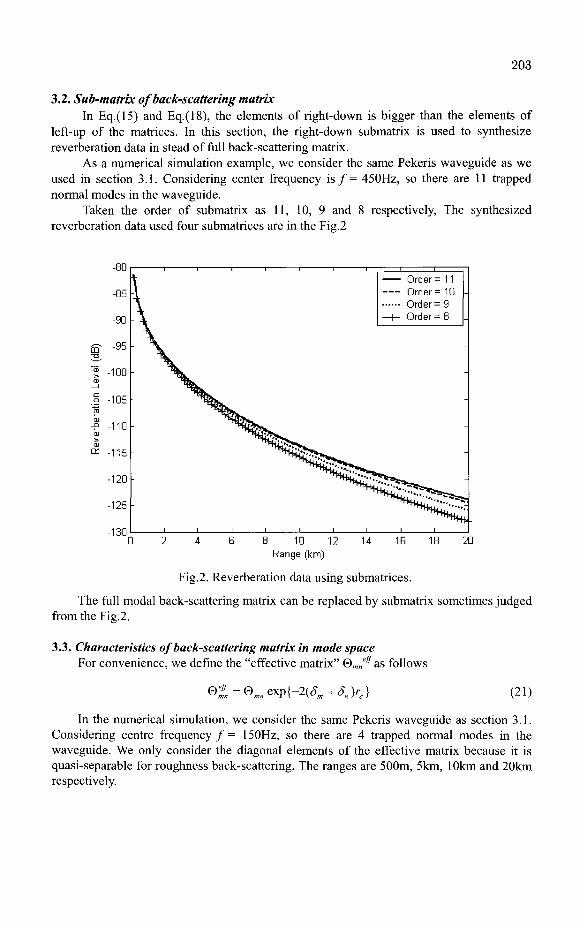
203
3.2. Sub-matrix of back-scattering matrix In Eq.(15) and Eq.(18), the elements of right-down is bigger than the elements of
left-up of the matrices. In this section, the right-down submatrix is used to synthesize reverberation data in stead of full back-scattering matrix.
As a numerical simulation example, we consider the same Pekeris waveguide as we used in section 3.1. Considering center frequency i s / = 450Hz, so there are 11 trapped normal modes in the waveguide.
Taken the order of submatrix as 11, 10, 9 and 8 respectively, The synthesized reverberation data used four submatrices are in the Fig.2
8 10 12 Range (km)
Fig.2. Reverberation data using submatrices.
The full modal back-scattering matrix can be replaced by submatrix sometimes judged from the Fig.2.
3.3. Characteristics of back-scattering matrix in mode space For convenience, we define the "effective matrix" ®m„eff as follows
© * = © m „ e x p { - 2 ( ^ + ^ K } (21)
In the numerical simulation, we consider the same Pekeris waveguide as section 3.1. Considering centre frequency / = 150Hz, so there are 4 trapped normal modes in the waveguide. We only consider the diagonal elements of the effective matrix because it is quasi-separable for roughness back-scattering. The ranges are 500m, 5km, 10km and 20km respectively.

204
Fie.3.rc = 500 m. Fig.4. rc = 5 km.
Fig.5. rc = 10 km. Fig.6. rc =20 km.
The results(Fig.3-Fig.6) show that: 1) in near distance, the value of back- scattering matrix elements inclines towards high modes. The matrix is similar to highpass filter; 2) in middle distance, the value of back-scattering matrix elements inclines towards middle modes. The matrix is similar to bandpass filter; 3) in far distance, the value of back-scattering matrix elements inclines towards low modes. The matrix is similar to lowpass filter. This phenomenon is caused by mode attenuation in shallow water waveguide.
4. Inversion of Modal Back-Scattering Matrix Extracting the bottom back-scattering information from reverberation data in
shallow-water waveguide is an attractive but difficult issue. In this section, two kinds of methods were proposed. One has a priori assumption; the other has no a priori assumption. They were called separable inversion and unseparable inversion of modal back-scattering matrix[ll]. 4.1 Numerical simulation of inversion of modal back-scattering matrix
First, make an assumption that the modal back-scattering matrix ®m„ is separable (Eq.l)
Then, make mode-filtering of the reverberation field. When the receiving vertical array is weighted by thej'-th mode function, we have

205
Psj(z0,rc) = lps(z,z0,rc)^(z)dzr
= f ^ f ^ o M , ^ ) • Snj • ^(zH)jArj(x)e,(^')xdX (22)
Taking only the non-interference term of the reverberation intensity as the averaged intersity
j M
Ij(z0,rc) = 7 ^ 2 > " ( z o ) © > , exp{-2(<5„ + Sj)re) k(jr
c n
(23)
Letj = l ,2
72 exp(-2£2rc)@2
Eq.(24) can be transformed to the following equation
Q 2 = ( / 2 _ ) ( exp ( -2^ , r c ) ) Q i
/, exp(-2£2rc)
And
0 3 = ( ^ ) ( ^ = ^ ^ ) © 1 /, exp(-2£3rc)
© M = ( ^ L ) ( M w e x p ( - 2 y c ) ) 0
Ix exp(-2£Mrc)
Integrated (25),(26),(27) and (23), we can get ©,, 02> 03> back-scattering matrix 0m„ using the separability(Eq.l).
Neglecting the dispersion effect, we have
(24)
(25)
(26)
(27)
and 0M. At last, get the modal
j M
Ij(z0,rc) = -^-^(zoy®„ exp{-2(Sm + Sj)re} Krc m
(28)
In Eq.(28), we have assumed that the unperturbed stratified waveguide is known, which means that ®mJ is the only unknown.
If, for each filtered modal reverberation intensity 7,, we change the source depth zs M times: ZS\^S2,"'^SM, then we will have MxM equations for solving the MxM unknown ®mJ
In the numerical simulation, we consider the same Pekeris waveguide as section 3.1. And take the roughness back-scattering as an example, its roughness parameters is: a = 0.1m, xo = 6m
The back-scattering matrix used to synthesize reverberation data is Eq.(15). And the inversed back-scattering matrix using separable method is
-52.9640 -48.1760 -46.2087 -45.3440"
Qsep -48.1760 -43.3880 -41.4207 -40.5560
-46.2087 -41.4207 -39.4533 -38.5886
-45.3440 -40.5560 -38.5886 -37.7239
(29)
The inversed back-scattering matrix using unseparable method is

206
s^\ unsep (30)
•52.9126 -48.1497 -46.2195 -45.3982"
-48.1497 -43.3745 -41.4262 -40.5837
-46.2195 -41.4262 -39.4511 -38.5774
-45.3982 -40.5837 -38.5774 -37.6677
At last, we get the separable inversion error and unseparable inversion error. The separable inversion error is (dB)
i©< • ©
0.0515
0.0264
0.0108
0.0542
0.0264
0.0135
0.0055
0.0277
The unseparable inversion error is (dB) "0.0
107^ • • 0
0.0108
0.0055
0.0022
0.0112
0.0542
0.0277
0.0112
0.0562
0.0 0.0
0.0 0.0 0.0
0.0 0.0 0.0
0.0 0.0 0.0
0.0
0.0
0.0
0.0
(31)
(32)
4.2. Inversion of modal back-scattering matrix from experiment data Reverberation data were collected in a reasonably flat shallow-water area in South
China Sea. A vertical line array was deployed to record monostatic reverberation from explosive charges. The explosive charges denoted at a depth of 7m. The vertical array contained 32 hydrophones, which were spaced from 7m to 69m. The sound speed profile measured during experiment is shown in Fig.7. The depth of the experiment sea area is 88.84m.
o
10
20
30
1 40
| 50
60
70
First Time Second Time
1529 1529.5 1530 1530.5 Sound Speed (m/s)
Fig.7. Sound speed profile.
Firstly, the separable inversion of the back-scattering matrix was presented. The separable inversion include following six steps:
The first step: make frequency filtering of the reverberation data, the center frequency

207
i s /= 200Hz The second step: make mode-filtering of the reverberation data The third step: get the I/j=l,2,---,M) The fourth step: get the ratio of ®m(m=l,2,---,M) The fifth step: calculate the ©i The sixth step: get the back-scattering matrix
&sep =
-82.9903
-82.6730
-82.3185
-76.6115
-75.0499
-65.9585
-82.6730
-82.3557
-82.0012
-76.2942
-74.7326
-65.6412
-82.3185
-82.0012
-81.6466
-75.9397
-74.3781
-65.2867
-76.6115
- 76.2942
-75.9397
-70.2327
-68.6712
-59.5797
-75.0499
-74.7326
-74.3781
-68.6712
-67.1096
-58.0182
-65.9585
-65.6412
-65.2867
-59.5797
-58.0182
-48.9268
(33)
Then, the unseparable inversion of the back-scattering matrix was discussed. The reverberation intensity can expressed as:
T MM
I(z0,z,rJ = -^^fi(z0)®mifi(z)vq>{-2(Sm+Sn)rc} (34) kDrc m n
The number of trapped mode in the waveguide is M=6, the unkown parameters the back-matrix is M-(\I2)(M-M)=2\
x,
0 :
x g
x1 2
x 1 3
x 1 4
x1 5
(35)
Using 21 channels of receiver array, we can get the unseparable back-scattering matrix
©"
-84.9205
-78.9090
-81.4483
-80.5997
-77.7279
-67.0755
-78.9090
-76.6619
-77.6056
-73.0682
-67.7421
-56.3842
-81.4483
-77.6056
-74.9338
-73.0582
-80.4350
-80.5997
-73.0682
-73.0582
-72.9733
-71.1268
-60.9133 -53.2428
-77.7279
-67.7421
-80.4350
-71.1268
-71.2151
-51.7836
-67.0755
-56.3842
-60.9133
-53.2428
-51.7836
-46.2848
(36)
5. Conclusion In this paper, the normal mode model of reverberation in shallow-water waveguides
has been presented based on Born approximation. Then characteristics of the modal back-scattering caused by (1) the roughness of the bottom interface and (2) the volume inhomogeneities under the interface are discussed. The back-scattering matrix due to roughness is quasi-separable; and the back-scattering matrix due to inhomogeneities is unseparable. In the certain condition, the full back-scattering matrix can be replaced by its submatrix. In mode-space, 1) in near distance, the value of back- scattering matrix elements inclines towards high modes. The matrix is similar to highpass filter; 2) in middle distance,

208
the value of back-scattering matrix elements inclines towards middle modes. The matrix is similar to bandpass filter; 3) in far distance, the value of back-scattering matrix elements inclines towards low modes. The matrix is similar to lowpass filter. This phenomenon is caused by mode attenuation in shallow water waveguide.
Two approaches of inversion of the matrix from reverberation data are proposed. One is separable inversion method, the other is unseparable method. Examples of the inversed result of the two inversion methods are shown both for numerical simulation and experiment.
Acknowledgements This work supported by the National Science Foundation of China under Grant No
10474111 and by Funds of Header of Institude of Acoustics(CAS) under Grant No S2004-10
References [I] G. L. Jin, R. H. Zhang and X. F. Qiu, "Characteristics of shallow water reverberation and inversion for bottom properties", Proceedings of SWAC, Ed. Zhang and Zhou, 303-308, 1997 [2] T. F. Gao, "Relation between waveguide and non-wave guide scattering from a rough interface", Acta Acust. 14, 126-132(1989) [3] D. J. Tang, "Shallow-water reverberation due to sediment volume inhomogeneities" (to be published) [4] F. G. Bass and I. M. Fuks, Wave Scattering from Statistical Rough Surface, Pergamon Press, 1979 [5] A. N. Ivakin, "A unified approach to volume and roughness scattering", J. Acoust. Soc. Am. 103, 827-837(1998) [6] D.D. Ellis and P. Gerstoft, "Using inversion technique to extract bottom scattering strength and sound speed from shallow-water reverberation data", Proceedings of 3rd
ECUA, Ed. By J. Pappadakis, Vol.1, 320-325,1999 [7] V. M. Kurdryashov, "Low-frequency reverberation in shallow-water Arctic Seas", Acoustical Physics, 45, 320-325, 1999 [8] Ji-Xun Zhou and Xue-Zhen Zhang, "Shallow-water acoustic reverberation and small grazing angle bottom scattering", Proceedings of SWAC, Ed. Zhang and Zhou, pp.315-322, 1997 [9] E.C.Shang, T.F.Gao, and D.J.Tang, "Extraction of Modal Back-Scattering Matrix from Reverberation Data in Shallow-water Waveguide. Part I — Theory", Theoretical and Computational Acoustics 2001, pp.67-74, Ed. E. C. Shang, Qihu Li and T. F. Gao, 2001, Beijing [10] L. Brekhovskikh, Ocean Acoustics, Moscow, HAYKA, 1974, Ch.4 [II] J.R.Wu. "Doctoral Disertation" (2005, IOA, Beijing)

NEW METHODS OF SCATTERING COEFFICIENTS COMPUTATION FOR THE PREDICTION OF ROOM ACOUSTIC PARAMETERS
XIANGYANG ZENG Institute of Environmental Engineering, PB58, Northwestern Polytechnical University,
XVan, 710072, China
E-mail: zenggxy @nwpu. edu. en
CLAUS LYNGE CHRISTENSEN ODEON A/S c/o Acoustic Technology, Technical University of Denmark, DK-2800, Denmark
JENS HOLGER RINDEL Department of Acoustics Technology, Technical University of Denmark, DK-2800, Denmark
To include the sound scattering caused by limited size of surfaces in room acoustic computer simulations, some model for scattering must be included in room acoustics computer models. A large concert hall usually contains a variety of small and complex surfaces and it is not practical to obtain accurate scattering coefficients of all these surfaces. Even if these frequency dependent coefficients could be obtained in the design phase, the modeling process would become more time consumed and increase the cost of design. In such a case, the appropriate simplification of the model and the definition of scattering coefficients by experience will become important. But in some other cases, calculation of a detailed model is necessary and possible. For these different cases, practical methods to define or calculate scattering coefficients, which include a new approach of modeling surface scattering and scattering caused by edge diffraction, have been presented. The predicted and measured acoustic parameters have been compared in order to testify the practical approaches recommended in the paper.
1. Introduction
Scattering has been validated to be one of the most important properties of sound in enclosed spaces [1-3]. Scattered reflection can improve the uniformity of a reverberant field and reduce the risk of areas of poor acoustics within a room. Surface scattering has found a role in dispersing reflections which are causing echoes or coloration [4]. The first international round robin test of computer modeling software has clearly indicated that inclusion of scattered reflections is an important factor in achieving good simulation results [5]. The investigations carried out by Hodgson [1], Dalenback [2] and Lam [3] have shown that the scattered reflections will not only affect the accuracy of the calculation of acoustical parameters, but also have influence on the quality of auralization.
Scattering coefficient is usually used to describe the scattering property of walls. It has been found that the coefficient is not only dependent on surface material, frequency of sound source, but also dependent on the geometry of the computer model [6]. It is possible for different computer models to get different calculation results on condition that the same scattering coefficients are used. This makes how to obtain the scattering coefficient a key problem. One way is direct measurement [7]. Another is to define it based on experience [8]. It can be found that the direct measurement is not practical for an arbitrary surface. This requests the users to be room acoustics experts, thus will limit the application of the program.
209
210
In this paper, rooms are divided into two groups: large and complicated rooms; small and simple rooms. For both cases, a method to consider both scattering due to surface property and scattering caused by edge diffraction has been applied. Practical methods to define the model and the scattering coefficients when using the program ODEON and other similar packages in both room cases have been given.
2. Current Methods for Modeling Surface Scattering
The basic idea to consider sound scattering in program ODEON is that the reflected energy can be divided into two parts at a surface: specular and scattered. Their relation can be denoted by the absorption coefficient CC and the scattering coefficient S
(l-s)(l-a) + a + s{\-a) = \ (l) The randomized ray propagations and secondary sources have been combined to
simulate the scattering. Instead of separating the ray tracing process into two parts, the model uses only a single ray tracing process for each ray. Furthermore, using the secondary sources to model radiation from the surface reflections to the receiver means that it is no longer necessary to check the validity and visibility of the image sources, thus reducing the computation time. However, the image sources in the model may not be the purely specular images. Even when the scattering coefficient is set to be zero, there is still some scattering that has been modeled. And it will reduce the effect of specular sound. To solve the problem, a factor named transition order (TO) has been defined, which can limit the scattering calculation only to those reflections having orders higher than TO. This scattering model has been applied into ODEON from version 2.5 to version7.0, and has been validated to be an efficient model.
The scattering coefficient used in the current model mainly considers the surface scattering due to material property and the TO can take into consideration the shape or structure of the acoustic room [6]. However, it has been found out that sound scattering is also dependent on the distance from the receiver to the edge of some small surfaces where diffraction usually occurs. This means it is not enough to take into account only the scattering due to surface property. Especially at low frequency and in the case where there are many varied small surfaces, the scattering caused by edge diffraction becomes more important and need to be calculated separately.
In the following section, the method to define a scattering coefficient combining both parts of scattering will be described at first. And then practical recommendations to define scattering coefficient for both kinds of rooms will be given.
3. Practical Methods to Define Scattering Coefficient
3.1. A new method for the calculation of scattering coefficient
To consider surface edge diffraction, we take a small panel as an example, which is shown in Fig.l. S,S' are the original sound source and image source, R is the receiver. It can be derived that the limiting frequency is [9]

211
/ „ = • c-d
(2) 2Acos<9
where c is the sound speed, A is the area of the small surface and d is the characteristic distance, which can be calculated from
2dj • d2 d =
dx +d2
(3)
S" R
Figure 1. Sound reflection from a small surface.
Above the limiting frequency, the diffraction losses can be considered negligible, while below the limiting frequency, it is
/ AL = 201og10 / .
(4)
This means at frequency higher than the limiting frequency, the sound energy can be thought totally specular and below the limiting frequency the scattering energy due to diffraction increases rapidly (6dB per octave band). This part of scattered energy can be represented by a factor sD, which can be calculated from
=i-(A2=i-(2/-A;osV (5)
Therefore, the total scattering coefficient s can be calculated from
s = \-(l-sD)i\-ss) (6)
Where sD is the factor related with distance from receiver to the edge of a surface and ss\s the scattering coefficient due to the surface property (defined in ISO/ FDIS17497-1).
Then the new direction of a reflected ray can be determined according to the value of s. If 5=1, the reflected ray will propagate in a scattered way which can be calculated according to Lambert's law; if 5=0,the reflected ray will propagate in a specular direction and can be easily obtained from Snell's law; if s is between 0 and 1, a new reflected direction can be determined by using s a sa weighting between the pure specular direction and scattered direction [10].

212
The above algorithm has combined the scattering due to edge diffraction and scattering due to surface property, therefore, it can reduce the influence of the scattering coefficient due to surface, which usually has to be defined according to the subjective experience of users.
3.2. Methods to define scattering coefficients for different rooms
For the case there are a variety of small and complex surfaces the computation will become more time consuming and it is also impossible to obtain the frequency dependent scattering coefficients due to surface property for all the surfaces. But in other cases, especially when the low frequency sound is more important, the detailed room model has to be considered. Therefore, we suggest two different ways to deal with small surfaces in large concert halls and small rooms. A. Small and simple rooms
For such kind of rooms, the number of main walls is usually small and the diffuser arrays may distribute in a few walls to achieve special acoustics effect. For instance, a studio room may need better acoustic behaviors at low frequency bands. It is required that some walls have to be equipped with special diffusers to counterbalance the weak scattering due to the simple structure of the room. On the other hand, as the sources or receivers are close to the reflector, which will produce strong reflections, considering the detailed structure of the model is necessary.
In this case, one scattering coefficient due to surface ss can be assigned to all these small surfaces. The recommended value is between 0.01 and 0.05. The scattering coefficient due to surface then will be combined with the part representing the scattering caused by surface edge diffraction.
In offices or classrooms, there is furniture such as tables and shelves. If a table plate is close to a source or receiver point, it likely to produce a strong reflection at the receiver, so it also should be included in the model. B. Large and complicated rooms
For a large artistic room, the shape and its interior structure are usually complicated. It is likely to contain too many small surfaces and to establish a model with such a degree of detail is likely to be a waste of time. It is recommended to simplify the real room when turning it into a visible computer model. That means some detailed parts of the walls may be deleted. But for such kind of walls the comparatively bigger scattering coefficients should be defined. The value is usually defined bigger than 0.3 and smaller than 0.8.
There are some guidelines for the simplification: (1) Curved surface. Curved surfaces have to be approximated by dividing them into
plane sections. How finely to subdivide depends on the type of curved surface and how important the surface is. Using many surfaces in the model will make the model visually complex, and increase the probability of errors in the model, typically small leaks becomes a problem. Subdivisions about every 10° to 30° will probably be adequate to reproduce focusing trends, without excessive numbers of surfaces.
(2) Audience area. Modeling each step between the rows in an audience area is not recommended. The audience area can be simplified a lot without compromising the quality of the results. However, this rule does not apply to open-air theatres.

213
(3) Podium on stage. The guideline is the same as that for the audience area. Rather than modeling each step of the podium, the podium can be simplified into a few sloped surfaces.
4. Prediction of Various Models
4.1. Conditions of experiments
A. PTB studio
The PTB studio, which was used to test different computer models in international round robin, has been chosen as an example in this paper. Two computer models for the studio have been designed for ODEON, named "simple" and "detailed" respectively, see Fig.2.
There are 70 surfaces in the simple model and the total surface area is 421 m2. For the detailed model, there are 268 surfaces and the total surface area is 450 m2. In the simple model the small diffusers on the ceiling and one wall have been neglected. The omni-directional point source is located at (x,y,z) = (1.5,3.5,1.5) and three receivers are: Rl (-2.00, 3.00, 1.20), R2 (2.00, 6.00, 1.20), R3 (0.00, 7.50, 1.20). The total ray number is 10000 and the transition order is 0. The scattering coefficients of various surfaces are listed in table 1. The measurement results are the mean value of 18 participants.
(a) (b)
Figure 2. PTB studio (a) simple model (b) detailed model.
To validate the scattering method presented in the paper, it has been compared with the old method applied in the ODEON ver7.0. Three cases have been studied: (1) simple model, old scattering method; (2) simple model, new scattering method; (3) detailed model, new scattering method. The acoustic parameters C80, T30, Ts, EDT, LF8o, D50 and G have been modeled and compared with the measured results.

214
Table 1. Scattering coefficients for PTB studio model.
Case
Simple model Old method
Simple model New method
Detailed model New method
Surface Parquet
Wilhelmi Curtain(open)
Studio wall Window glass Wood absorber
Ceiling Ceiling
Wood absorber Other surfaces
All other surfaces
Scattering coefficient 0.20 0.30 0.48 0.20 0.10 0.95 0.95 0.85 0.85 0.02
0.02
B. Elmia concert hall
Two kinds of models of the Swedish concert hall Elmia were set up in ODEON. One is simplified and another is in detail. See Fig. 3.
There are 94 surfaces in the simple model and the total surface area is 4409 m2. For the detailed model, there are 470 surfaces and the total surface area is 4932 m2. In the simple model the small diffusers on the side faces have been simplified. The omni-directional point source is located at (x,y,z) = (8.5, 0.0, 25.5) and six receivers are: Rl (13.8, 0.0, 24.9), R2 (12.9, 10.5, 28.7), R3 (19.9, 5.1, 26.1), R4 (25.5, -4.9, 27.5), R5 (24.8, 11.9, 29.1), R6 (37.80, 6.40, 131.85). 10000 rays have been used to calculate the acoustics parameters C80, T30, Ts, EDT, LF80, D50 and G. The transition order is set to be 4 and the scattering coefficients of various surfaces are listed in table 2. The predicted acoustic parameters have been compared with those of measurements.
(a) (b)
Figure 3. Elmia concert hall (a) simplified model (b) detailed model.

Table 2. Scattering coefficients for Elmia model.
model
Simplified model
Detailed model
Surface Audience area
Simplified surfaces Other surfaces Audience area Side reflectors
Ceiling Other surfaces
Scattering coefficient 0.60 0.30 0.02 0.60 0.35 0.30 0.02
4.2. Results and discussion
A. Accuracy of different scattering models
For the PTB studio, the mean errors of the three cases at 6 frequency bands are listed in table 3. For the Elmia concert hall, the mean errors of the two cases at 6 frequency bands are listed in table 4.
Table 3. Average errors of at three receiving positions in PTB studio.
Simple model-old method
Simple model-new method
Detailed model-
new method
Parameter
Qo(dB) G(dB) T30(s)
C80(dB) G(dB) Ts(s)
C80(dB) G(dB) T30(s)
Frequency (Hz) 125 1.8 2.5
0.17 1.6 2.0
0.16 3.0 0.1 0.16
250 1.1 2.2
0.27 1.1 1.8
0.20 1.2 0.7 0.09
500 0.2 1.5
0.13 0.1 1.1
0.09 0.4 1.0
0.03
1000 0.1 1.3
0.06 0.2 0.8 0.04 0.4 0.7
0.07
2000 0.2 1.3
0.12 0.1 0.8 0.06 0.3 0.6 0.04
4000 0.1 1.0
0.06 0.1 0.8
0.12 0.4 0.7 0.03
Table 4. Average errors of six receiving positions in Elmia concert hall.
Simple model-new method
Detailed model-
new method
Parameter
C80(dB) G(dB) T30(s)
Qo(dB) G(dB) T30(s)
Frequency band(Hz) 125 2.9 1.0
0.32 3.7 1.6
0.42
250 0.8 2.2
0.13 1.3 1.8
0.33
500 1.4 1.1
0.18 0.8 0.9
0.23
1000 1.2 0.8
0.09 0.9 0.4 0.20
2000 1.3 0.7
0.15 0.9 0.6 0.27
4000 1.7 1.3
0.23 0.8 1.8
0.28

216
Table 3 shows that when using the new method for the simple model, the results are better than those of the old method. And when using the new method for the detailed model, the results are the best except for C80. The predicted C80 is bigger than the measured ones and the difference is much bigger at low frequency bands when using the new method for the detailed model. This may indicate more early sound energy is collected because of the reflection and diffraction from those small surfaces that have not been considered in the simple model.
Table 4 has shown that the prediction accuracy of C80 and G of the two models is comparable. Both of them can get acceptable results at different frequency bands. But for the parameter T30, the simple model can obtain better results at all frequency bands. This means the simplified model can also achieve satisfied results. According to the results of some other parameters like LF80, Ts and D50, it also can be concluded that the accuracy of these two models is approximate. B. Influence of TO on the prediction accuracy
As in the ODEON model, the value of TO is also a important factor which can affect the scattering modeling, different TO cases have also been calculated. C8o and EDT are investigated in this paper. Table 5 and 6 have given the results.
It can be found that when the TO is set to be zero or 1 for the PTB studio model, the accuracy is better. From TO=2 to TO=5, the average error of the six frequency bands will exceed ldB. From table 6, it can be found that when TO=4 or TO=5, the mean errors at all frequency bands are smaller. These results may indicate that for the typical concert hall the TO should be higher than 3, while for approximately proportionate rooms zero or 1 are the best choice for TO.
Table 5. TO and predicted Cso(dB) in PTB detailed model.
f(Hz) TO=0 TO=l TO=2 TO=3 TO=4 TO=5
Measured
125 8.7 8.8 9.1 9.5 9.3 8.8 5.7
250 4.6 4.8 5.4 6.0 6.3 6.1 3.5
500 3.4 3.8 4.3 4.8 5.1 5.0 3.1
1000 4.3 4.6 4.9 5.2 5.3 5.1 3.9
2000 3.5 3.7 4.1 4.2 4.3 4.2 3.3
4000 4.7 4.8 4.9 4.8 4.7 4.6 4.4
Table 6. TO and predicted EDT(s) in Elmia simple model.
f(Hz) TO=0 TO=l TO=2 TO=3 TO=4 TO=5
Measured
125 1.47 1.86 1.88 2.06 1.91 2.02 2.10
250 1.86 1.66 1.88 2.09 2.34 2.23 2.33
500 1.92 1.70 1.98 1.98 2.15 2.08 2.19
1000 1.89 1.70 1.84 1.75 2.44 2.10 2.22
2000 1.76 1.74 1.90 1.72 2.25 1.93 2.04
4000 1.50 1.14 1.40 1.58 1.86 1.96 1.70

217
C. Computation time and model complexity
From table 7, it can be found that with the same number of rays, the computation time of the detailed and the simple PTB studio model is very close. But as concluded in section "A", there is an obvious increase of accuracy. It means the new method for the detailed model is more practical than that for the simple model. For the Elmia concert hall this is more obvious. The computation time has increased to 525% if the detailed model is used, but the accuracy has almost no increase.
Table 7. Comparison of different models.
Total surfaces Total area(m2)
Total rays Source number
Receiver number Computation time(s)
PTB simple
70 421
20000 1 3
34
PTB detailed
268 450
20000 1 3 33
Elmia simple
94 4409 20000
1 6
40
Elmia detailed
470 4932 20000
1 6
211 *the CPU frequency of the computer is 2.0GHz.
5. Concluding Remarks
A scattering model has been presented and practical methods for the consideration of surface scattering when using room acoustics computer model ODEON. These methods are better than the conventional methods that only consider the scattering coefficient due to surface property.
For acoustic consultants or computer model users, it is also an important problem to realize the balance between the accuracy and design difficulty. Two different ways have been given for the two groups of rooms, and some rules have been recommended on the inclusion or simplification of small surfaces in rooms. The discussion of the paper has indicated that for large complicated rooms, it is practical to simplify model geometry, while for small rooms, it will be benefited from the calculation of detailed models.
The recommendation of scattering coefficient definition in various cases is as follows. If the geometry of a model has been simplified, the coefficient of the substituted surface should be a bit smaller than that determined by experience and usually between 0.3 and 0.8. If all the detail of a room is considered, each surface can be thought as smooth except for some special ones, therefore, the same scattering coefficient (ss) for all of these smooth surfaces can be set to be a low value from 0.01 to 0.05.
As for transition order, in a general way, it should be smaller than 3 in small and simple shaped rooms and in large concert hall, it is better to set the transition order around 4.

218
6. Acknowledgements
This work is partially supported by National Natural Science Foundation of China [no. 10404021] and the Fund for Outstanding Persons in Northwestern Poly technical University of China.
References
1. Hodgson M.R., Evidence of diffuse surface reflection in rooms, J. Acoust. Soc. Am. 89(1991)765-771.
2. Dalenback B.I.,Kleiner M. and Svensson P., A macroscopic view of diffuse reflection, J. Audio Eng. Soc. 42 (1994) 793-806.
3. Lam Y.W., On the parameters controlling diffusions calculation in a hybrid computer model for room acoustics prediction, Proc. IOA. 16 (1994) 537-544.
4. Antonio P.D. and Cox T.J., Diffusor application in rooms, Applied Acoustics 60 (2000) 112-143.
5. Vorlander M., International round robin on room acoustical computer simulations, ICA'95 (1995), pp. 689.
6. Lam Y.W., The dependence of diffusion parameters in a room acoustics prediction model on auditorium size and shapes, J. Acoust. Soc. Am.100 (1996) 2193-2203.
7. Mommertz E. and Vorlander M., Measurement of scattering coefficients of surfaces in the reverberation chamber and in the free field, ICA '95 (1995) 577-590.
8. Christensen C.L., Manual of ODEON room acoustics program version 7.0, 2003. 9. Rindel J.H., Acoustic design of reflectors in auditoria, Proc. I.O.A. 14 (1992) 119-
128. 10. Christensen C.L. and Rindel J.H., Predicting acoustics in classrooms, Inter-noise
2005 (2005) 1782.

AW 'orld Scientific
YEARS O F P U B L I S H I N G
1 1 — 2 0 0 8
6283 he ISBN 981-270-084-6
www.worldscientific.com


