DETERMINING THE ACTUAL HYDRAULIC RETENTION TIME OF A

CONSTRUCTED WETLAND CELL FOR COMPARISON WITH THE

THEORETICAL HYDRAULIC RETENTION TIME

BY

BRANDY HUNT

(Under the direction of Dr. Matthew Smith)

ABSTRACT

The design of constructed wetlands for wastewater treatment is based on

the hydraulic retention time, which is the most easily changed operational

variable in the design. This can be changed by the flow rate, decaying plant

matter, or sludge accumulation, because of changes in volume and depth. A

tracer study was conducted to determine the hydraulic retention time for cell one

of the Tignall Water Treatment Facility. According to the results of the study, the

average hydraulic retention time is approximately 7.7 days which indicates that

the hydraulic efficiency of the system is approximately 0.50, which is average

according to Persson et al. (1999), but other findings of the study, such as plant

density, indicate that the system may be beginning to decline. It is

recommended that wetland cell one be drained, dredged, and replanted.

KEYWORDS: Wastewater, Constructed Wetlands, Hydraulic Efficiency,

Hydraulic retention time

DETERMINING THE ACTUAL HYDRAULIC RETENTION TIME OF A

CONSTRUCTED WETLAND CELL FOR COMPARISON WITH THE

THEORETICAL HYDRAULIC RETENTION TIME

by

BRANDY HUNT

B.S.B.E., The University of Georgia, 1998

A Thesis Submitted to the Graduate Faculty of The University of Georgia in

Partial Fulfillment of the Requirements for the Degree

MASTER OF SCIENCE

ATHENS, GEORGIA

2002

© 2002

Brandy Hunt

All Rights Reserved

DETERMINING THE ACTUAL HYDRAULIC RETENTION TIME OF A

CONSTRUCTED WETLAND CELL FOR COMPARISON WITH THE

THEORETICAL HYDRAULIC RETENTION TIME

by

BRANDY HUNT

Approved:

Major Proffessor: Matt Smith Committee: Rhett Jackson

David Gattie William Tollner

Electronic Version Approved:

Maureen Grasso Dean of the Graduate School The University of Georgia December 2002

iv

Dedication

To Jill Davenport, thanks for the help, the data, the discussions. This is a better

thesis because of those discussions.

To Dr. Matthew Smith, thanks for the challenges and the occasional boot to the

head.

To every member of Watershed Assessment Office, past and present, I can

never thank you enough for the support and help you have given for the

first two years of the graduate student career.

To every member of the Environmental Quality Water Lab, I can also never

thank you enough for the support and help you have given me the last

year and a half.

To my Mom and Dad, thanks for always standing behind me and giving me the

tools I needed to survive the last four years of frustration that have been

my graduate school career.

To my friends, especially Mikey, Dan, Aimee, and Alexandra, I’ve been at this

as long as most of you have known me, and your support and kibitzing

have been appreciated.

To my husband, Christopher “The Tigger” Smith, thank you for being the most

caring, supportive human being it has been my pleasure to meet, love,

and marry. I promise, babe, the insanity is almost over.

v

Table of Contents

Page

SECTION

1.0 INTRODUCTION ...................................................................................... 1

2.0 LITERATURE REVIEW ............................................................................ 6

3.0 Methods.................................................................................................. 12

3.1 Choice of dye..................................................................................... 12

3.2 Calibration of the dye concentrations to the absorbance ................... 12

3.3 Dye degradation ................................................................................ 15

3.4 Prototype Run.................................................................................... 17

3.5 Experimental Run .............................................................................. 18

3.6 Climate Conditions............................................................................. 21

3.7 Bathymetry survey ............................................................................. 21

4.0 Results.................................................................................................... 24

4.1 Middle-Mixing zone grab samples ..................................................... 24

4.2 Hydraulic retention time analysis ....................................................... 26

4.3 Bathymetry survey ............................................................................. 30

5.0 DISCUSSION AND CONCLUSIONS...................................................... 35

6.0 REFERENCES ....................................................................................... 38

7.0 APPENDIX ............................................................................................. 39

1

1.0 Introduction

In the past, environmental engineers have relied on first order

approximations of rates of transformation, reduction, and the removal of

pollutants from water. However, because ecological process descriptions are

complex, close scrutiny must be paid to each of the above categories for a

complete understanding of the system as a whole. This particular project

examines the application of constructed wetlands within the larger category of

the treatment of municipal wastewater. While soils, sediments, microbes, and

macrophytes are all important to a constructed wetland, it is necessary to

understand the movement of water within the wetland, since hydraulic retention

time (HRT) is the basis for most wastewater treatment designs. (Kadlec 1994)

The movement of water within a constructed wetland can be influenced by

various interactions. A wetland may have excluded zones like plant and

accumulated sludge volumes (Kadlec 1994). Excluded zones are areas where

water is stagnating or otherwise not getting treated. These excluded zones are

taken into account during the design phase; however, when these zones

increase in volume, they become impediments to the treatment of the

wastewater. While interactions that influence the water budget, like precipitation

and evapotranspiration, can cause the wastewater to flow unpredictably through

the wetland, the excluded zones are the easiest interactions to control. There

are of course more interactions that can influence the movement of water, but

they cause unsteady flow patterns, which can be difficult to analyze in a

2

constructed wetlands hydraulic regime. This is because unsteady flow is almost

impossible to isolate and model. (Rash and Liehr 1999)

Tracer studies indicate that treatment in subsurface flow wetlands is more

influenced by velocity profile effects than by dispersion, and in free water surface

wetlands, velocity profiles can lead to a distribution of hydraulic residence times.

Velocity profiles are formed by friction, as the water flows over surfaces that slow

it down. The distribution of hydraulic residence times is originates because the

shortest residence time is experienced by water moving at the maximum velocity

in the profile. Hilton et al. (1998) found that for free water surface wetlands dye

concentrates in the top few inches of the water column, but over the course of

the study, the dye gradually spread vertically and longitudinally. Since this study

took place in Boston harbor, it is impossible to say that the dye was mixed well

when it was released, which is why Hilton et al. (1998) never considered the dye

well mixed. However, these findings were also confirmed by Werner and Kadlec

(2000) in a study of fresh water free water surface wetlands. (Werner and

Kadlec 2000)

In the tracer study conducted in Tignall, GA, there was an attempt to mix

the tracer dye in to the mixing zone at the inlet. This should have taken care of

velocity profile effects when the dye was added. Also, the mixing zone in the

middle of the wetland cell should have also negated velocity profile effects. This

will be discussed in more detail later.

Since the system in the Tignall, GA, has been running for several years,

the expected result of this study is that the mean hydraulic retention time differs

3

from the nominal retention time of the constructed wetland cell enough to

suggest that the cell is not adequately meeting design standards and, by

extension, treatment standards. The overall goal of this project was to

experimentally determine the mean hydraulic retention time of a constructed

wetland cell and to compare it to the nominal hydraulic retention time. Other

goals included determining how well the mixing zones are mixing.

This study takes place at the Water Reclamation Facility, in Tignall, GA.

The system consists of two Lemna cells and an aeration pond that pre-treats the

wastewater before it goes to the constructed wetlands system. The constructed

wetlands system consists of eight free water surface wetland cells that are

connected by a system of inlet and outlet structures that will allow for series,

parallel, or series/parallel flow. Each cell is 400’ by 60’, with three deep zones to

promote mixing. These deep zones will be referred to in this paper as inlet,

middle and outlet mixing zones according to its position in the wetland cell. The

flow rate for the period of time that the study took place ranged between 13

ft3/min to 16 ft3/min, so it is approximated as 14.5 ft3/min. This means that

approximate volume of the wetland cell was 160,776 ft3. Using information from

Precision Planning, this left the design depth at approximately 0.84 ft, and the

hydraulic retention time was approximately 15.5 days.

This study was done on the first wetland cell, which is one of the oldest

cells in the system, while the system was in series. Figures 1 and 2 on the

following pages shows the entire system, and how they are arranged.

4

Lemna pond

Partial mix aeration pond

Wetland cell 1

Figure 1. Schematic of the site

5

Figure 2. Schematic of the cells in relation to each other

6

2.0 Literature Review

Different particles of water remain in the constructed wetland for varying

amounts of time. This produces varying amounts of treatment. Persson (2000)

found that plug flow is considered the optimal flow, because all fluid elements

reside around the nominal residence time. When the particles of water are

recombined at the outlet, this will produce an overall level of treatment, which is

dependent on the average retention time. This is because the biological

processes that provide treatment are time dependent. (Werner and Kadlec

2000)

One of the primary ways of characterizing this behavior is to calculate the

nominal detention time, which is the average contact time in the wetland. This is

because changes in hydraulic retention time can be deliberately caused by

changes in depth and flow rate. Plant and accumulated sludge depths can cause

these changes to become uncontrollable. This is defined as tn = Q/V, where Q is

the flow rate and V is the design volume. The nominal detention time assumes

no stagnation, short-circuiting, or dead zones occur so the relationship to the

actual flow behavior in a mature cell is minimal. Another way to characterize a

constructed wetland is by saying that the mean hydraulic retention time times the

flow rate defines the active volume, Va, which is where the treatment actually

takes place (Simi and Mitchell 1999). (Rash and Liehr 1999)

An alternative way of looking at the detention time is to construct a

residence time distribution (RTD). This represents a probability density function

7

of the amount of time that a particle spends in the reactor and/or wetland. It is

scaled so that the integration of the curve is unity. The RTD function, or E(t), is

based on the flow rate and the effluent concentration of whatever the study has

used for a tracer, and to find a more accurate representation of the detention

time one must integrate the expression tE(t)dt. RTD is most often used in

constructing models, which will be briefly discussed later (Rash and Liehr 1999)

Since most constructed wetlands are designed as a sort of biochemical, or

biological, reactor, it seems prudent to go through some of these definitions

before going further. It has become apparent from a variety of research projects

that wetland reactors do not fit any particular set of limiting conditions and seem

to be an intermediate between a continuously stirred tank reactor (CSTR) and a

plug flow reactor (PRF) (Kadlec 1994). If completely mixed, all water particles, or

parcels, have an equal probability of leaving the wetland at a given moment, and

the system is thought of as a CSTR. If there is no distribution of times and all

parcels spend the same amount of time in the system, it is a PFR. Most

constructed wetlands are designed based on plug flow assumptions, which is an

ideal situation that does not often occur. Plug flow design has also been found to

result in over design (King et al. 1997). Deviation from plug flow can occur

because of channeling through preferential flow paths or exchanging of flow with

stagnant regions (Simi and Mitchell 1999). (Werner and Kadlec 2000)

In order to determine the average hydraulic retention time and gather

information for a residence time distribution (RTD), a tracer study is conducted.

The object of a tracer study is to build a tracer response curve. This curve is a

8

graph of the concentration of the tracer versus time. Care must be taken

determining the frequency of sampling, because a missed dip or peak can

introduce inaccuracy when calculating the mean hydraulic retention time (Werner

and Kadlec 2000). The mean hydraulic retention time is characterized by the

centroid of the distribution under the curve (Simi and Mitchell 1999).

The shape of the curve can imply information about what conditions exist

in the constructed wetland. An asymmetrical curve with an extended tail may

mean that there are dead zones and channeling (Simi and Mitchell 1999). The

presence of two separate peaks clearly indicates the presence of two parallel

paths, where the first peak indicates the shorter route (Batchelor and Loots

1997). A curve with a large standard deviation suggests the presence of short-

circuiting flow paths and flow re-circulating zones (Persson et al. 1999). Finally,

a large difference between the observed mean detention period and the nominal

detention period suggests the presence of zones of stagnation in the system

(Persson et al. 1999).

After graphing the tracer response curve, it is possible to find the retention

time distribution, or RTD. As stated above, the RTD is the distribution of times

that parcels of water spend in the constructed wetland. RTD is often used in the

modeling of the hydraulic retention time for a specific wetland. Considering the

wetland as a series of CSTRs and PFRs makes this acceptable. (Werner and

Kadlec 2000) While the data from this study can be used to construct such a

model, this study is more concerned with the actual hydraulic retention time of

the constructed wetlands.

9

One concept that will be used in this study is the idea of hydraulic

efficiency, λ. This efficiency is based on design standards, or how close the

wetland cell is to design specifications. Persson (2000) also defines the

hydraulic efficiency as “how well the incoming water distributes within the pond.”

This is a proportion that reflects the ability of the constructed wetland to distribute

the inflow evenly across the detention system and the amount of mixing or

recirculation. Dividing the mean hydraulic retention time by the nominal hydraulic

detention time derives this proportion. This proportion is also equal to the

effective volume divided by the design volume, which will aid the analysis of the

data. When stated in terms of volume, the proportion is referred to as e (Persson

2000). Persson et al. (1999) found that a good hydraulic efficiency is

characterized by a � higher than 0.75; satisfactory hydraulic efficiency is

characterized by a � between 0.50 and 0.75; and poor hydraulic efficiency is

characterized by a � less than 0.50. Most of the wetland designs in the Persson

et al. (1999) study had � of less than 0.50, but still give satisfactory treatment.

This could be because of the over design inherent in the plug flow models used

to design constructed wetland cells. (Persson et al. 1999)

Persson et al. (1999) evaluated thirteen different wetland designs using a

computer program called MIKE-21, which is a two dimensional depth integrated

hydraulic model that simulated the hydraulic regime based on length to width

ratios, impediments, and inlet and outlets. The layouts with the best hydraulic

efficiencies were an elongated pond, a pond with baffles, and a system with three

inlets and one outlet. The elongated pond’s length to width ratio was greater

10

than 4:1, or the results were to close to the pond layout that had a length to width

ratio of 3:1.

Another important factor in tracer studies is the tracer dye itself.

Comparative wetland studies demonstrate that bromide, lithium, and fluorescein

dyes are all approximately equivalent (Kadlec 1994). Before conducting this

study, bromide and fluorescein dyes were compared in the literature. Bromide is

often used because of its low background concentration in most soils, and its low

biological and chemical reactivity in a soil environment. Bromide concentrations

in ryegrass grown in well-drained soil were greater than that of ryegrass grown

on poorly drained soil close to wetland conditions. However, in soils with a

higher fertility, or more nitrogen, there was no difference (Schnabel et al. 1995.

The proper instrumentation was not immediately available to conduct any tests to

confirm this would be the case for the wetland cells in Tignall, GA. )

Rhodamine, as an example of fluorescein dyes, is fluorescent, resists

adsorption, and is detectable at very low concentrations (0.1 mg/L). It has been

reported to produce no major problems when released in low concentrations and

is light sensitive. Eventually, it degrades in sunlight and is no longer present in

the environment. Rhodamine concentrations are determined by extrapolation

from a standard curve of fluorescence units versus a range of standard

concentration. (Simi and Mitchell 1999)

For this study, a flourescein dye seems to be the best tracer dye. The

plant material does not absorb it, and it is detectable in small concentrations.

11

The type of dye used in this study will, according to the manufacturer, eventually

completely break down and not be noticeable to downstream inhabitants.

Once the mean hydraulic retention time is found, the effective volume can

be determined. Then suggestions can be given for increasing the hydraulic

retention time. Such suggestions could indicate that modifying the vegetation

layout or dredging the mixing zones which would immediately improve the

hydrodynamic conditions.

12

3.0 Methods

3.1 Choice of dye

The choice of dye had been discussed in the literature review. The use of a

flourescein dye was the best solution, but there are several types of flourescein

dyes. Rhodamine is a type of red dye that lasts about three to five days

according to the manufacturer; however, according to the HRT that the cells were

designed for, a dye that lasted longer was needed. It was decided that the

yellow/green dye distributed by Bright Dyes would be the best dye to use for the

following reasons.

1. The manufacturer states that the dye breaks down in seven days.

2. A spectrophotometer could be used to instead of a flourometer to analyze

the samples, thereby solving any scheduling conflicts with other

researchers. This also solves the problems of masking by other

chemicals.

3. It comes in several forms—the liquid form being the least messy and the

most desirable.

3.2 Calibration of the dye concentrations to the absorbance

The yellow/green dye is best seen in a spectrophotometer at 490 nm and

520 nm wavelengths according to the manufacturer. By using wastewater

without dye in it as the blank that the spectrophotometer needs to compare the

samples to, the change in absorbance is calibrated to the concentration in those

samples that have dye in them.

13

Using Beer’s Law, which states that if absorbance values are below

1.0000 a better linear relationship between absorbance and concentration is

found, it was decided that 520 nm was the best wavelength since at 520 nm the

more samples with absorbances below 1.0000 were found so that a better

calibration relationship could be obtained at this wavelength. All samples and

calibration sets have been analyzed at this wavelength. This has given

significant linear relationships between the concentration of dye in the samples

and the absorbance.

In the beginning, the calibrations were done at the beginning of the

experiment, but when replicating the experiment it was found that it is best to

calibrate each time the samples are retrieved from the ISCOs. Further, the

calibrations were divided into sets to increase the significance of the linear

relationship sought. These calibration sets where divided as follows:

1. 0.0, 0.2, 0.4, 0.6, 0.8, 1.0 mg of active dye/L,

2. 0.0, 2.0, 4.0, 6.0, 8.0,10.0 mg of active dye/L,

3. 0.0, 20.0, 40.0, 60.0, 80.0, 100.0 mg of active dye/L, and

4. 0.0, 200.0, 400.0, 600.0, 800.0, 1000.0 mg of active dye/L.

This provided significant linear relationships with R2’s ranging from 0.99 to 0.86,

which are very good for this type of calibration.

3.2.1 Initial dye concentrations

Previous experience with cell 4 had indicated that the concentration had to

be high, or the dye was too diluted to find with either a flourometer or a

spectrophotometer. Even at 350 mg active dye/L this held true. From the

14

calibrations, it was known that at 700 mg active dye/L the absorbances were

approximately 3.0 almost every time, which allowed for dilution. This was three

times what was needed to comply with Beer’s Law, so 700 mg active dye/L was

decided to be the most acceptable.

Working at the maximum design operating depth, the depth of the wetland

cell was approximately six inches deep and knowing that the mixing zones were

three feet deep, calculations revealed that the volume of the mixing zone was

about 7200 ft3 or 219.5 L. It required about three liters of dye to bring the inlet

mixing zone up to the target concentration.

3.2.2 Quality Control

Because the characteristics of wastewater are always changing, it is very

important to keep the calibration as current as possible. To this end, the

following procedure was used to insure that the relationship found in the

correlation remains as accurate as possible.

Every time samples were retrieved, another liter of wastewater was taken

as a blank sample for calibration and quality control. Then one 20 mL sample

was chosen from each sampler set. After the 3 mL were taken for analysis, the

sample was spiked with enough dye to bring a 3 mL volume without any dye in it

to a 5 mg active dye/L. After each sample is analyzed, the spiked sample’s

absorbance was compared to the appropriate absorbance for that concentration

using:

%D = ((true value-found value)/true value) 100,

where %D = percent difference, true value = absorbance of the spiked sample, and

15

found value = absorbance according to the calibration relationship. If the percent difference is more than 5%, then the calibration was redone with

the new wastewater blank, and the samples re-analyzed.

3.3 Dye Degradation

This experiment was set up to check the manufacturer’s claims as to how

long the dye existed in the wetland cell. Since the prototype run had been

affected by the recycling of wastewater, it seemed relevant to also test how

quickly the dye degraded. Two aquariums were borrowed from the

Environmental Water Quality lab. By placing the aquariums in the cell, the water

should undergo all of the conditions of the dye in cell 1, except flow. This will be

used to gauge how long Experiment 2 should run and examine degradation rates

The aquariums were filled with wastewater from wetland cell 2, and dye

was added so that each would have a concentration of 700 mg active dye/L. The

aquariums were placed in the inlet-mixing zone of cell 2, in case of over flow, and

left for the duration of the study. Samples were taken from each aquarium at the

same time that samples were picked up from the ISCO samplers for Experiment

2. These samples were analyzed using the spectrophotometer and were used

as a measure of how the dye degraded in the wetland cell.

The dye in this experiment did not actually degrade the way the

manufacturer explained it would. According to the manufacturer, the dye

degrades as the BOD in the wetland cell does, or at most in twenty-one days.

The following tables, however, show that the manufacturer could be wrong.

16

Table 1. Absorbance from the dye in Aquarium 1

Date Absorbance Concentration, mg/L 02/22/02 2.9341 700.46 02/26/02 3.0060 717.63 02/28/02 3.0243 722.00 03/08/02 2.9467 703.47 03/12/02 2.5970 612.00

Table 2. Absorbance from the dye in Aquarium 2

Date Absorbance Concentration (mg/L) 02/22/02 3.0909 737.8964 02/26/02 3.1690 756.5414 02/28/02 3.1546 753.1037 03/08/02 2.3290 556.0066 03/12/02 0.9191 219.4185

Aquarium 2 overflowed on 3/4/2002, and both aquariums were iced over

so that it was impossible to get a sample. By 3/9/2002, there was no more dye in

the samples from the outlet-mixing zone. As can be seen there was little

variation in the absorbances from aquarium 1, and what variation there is could

be the result of evaporation or dew. Therefore, it can be suggested that there

was no actual dye degradation going on in the wetland cell, unless flow plays a

more important part than any other variable.

Using the relationships, C = C0e-kt, where k is the rate constant for dye

degradation, and C0 is the original concentration of 750 mg active dye/L, Figure 3

is generated. Using linear regressions, the R2 for Aquarium 1 is 0.46, and the R2

for Aquarium is 0.58. This suggests that degradation did not occur during the

experiment, or if it did occur, not as the manufacturer expected.

17

-0.35

-0.3

-0.25

-0.2

-0.15

-0.1

-0.05

0

0.05

0 2 4 6 8 10 12 14 16 18

Time, days

ln(C

/Co)

Aquarium 1 Aquarium 2

Figure 3. The relationship between time and the degradation of the dye.

3.4 Prototype run

The first sampling run was approximately 3 weeks long, and occurred

during the fall of 2001. The dye was added 10/9/01. To provide the appropriate

mixing, the dye was introduced to system via the weir station above the wetland

cells. An ISCO sampler will be used to automate the sampling process, and the

tracer used was the FLT Yellow/Green, a specially formulated version of

flourescine dye. It was reported to not absorb to organic matter and to exist for

five to seven days. The sampling frequency was to occur in the following

manner: every two hours when the tracer is expected to go through the sampling

point, and every four hours during those times when the tracer is not expected to

go through the sampling point. However, after the first run, this sampling

18

frequency was revised to reflect difference between the design hydraulic

retention time and what is actually going on in the wetland cells. A sampling

point was set up in the last mixing zone of the wetland cell. Each sample was

about 20 mL.

There were six sampling points set up in the middle-mixing zone. These

were in pairs of three on either side of the middle-mixing zone. One pair will be

at 15’, the next at 30’, and the last at 45’. These will used to determine whether

or not the mixing zone is actually doing what it is supposed to be doing—mixing

the wastewater to improve homogeneity of the wastewater to improve treatment.

The experimental run did provide good data for the mixing zone analysis;

however, as was found out after the prototype run, the operator of the facility was

recycling wastewater. This recycled the dye, which as explained above, was not

degrading as expected. However, the middle mixing zone data was still good,

which was fortuitous because of some mechanical problems during the

experimental run. The samples taken from the middle mixing zone could be

used to test the claim that the mixing zone increased mixing of the wastewater,

because the absorbances could be analyzed to show if there was any decrease

in difference in the wastewater on the outlet side of the mixing zone.

3.5 Experimental Run

The second sampling run was about 18 days long and occurred during the

late winter of 2002. The dye was added 2/18/02. To provide the appropriate

mixing, the dye should be introduced to system via the weir station above the

wetland cells. An ISCO sampler will be used to automate the sampling process.

19

The Environmental Water Quality Laboratory had several programmable ISCO

6700s available. An ISCO sampler is programmable with the capacity to hold

twenty-four bottles. The tracer used will be the FLT Yellow/Green, a specially

formulated version of flourescein dye. It was reported to not absorb to organic

matter and to exist for five to seven days. The sampling frequency should occur

in the following manner: every two hours when the tracer is expected to go

through the sampling point, and every four hours during those times when the

tracer is not expected to go through the sampling point. A sampling point was

set up in the last mixing zone of the wetland cell. Each sample was about 20 mL.

There were six sampling points set up in the middle-mixing zone. These

were in pairs of three on either side of the middle-mixing zone. One pair will be

at 15’, the next at 30’, and the last at 45’. These sampling points were used to

determine whether or not the mixing zone is actually doing what it is supposed to

be doing—mixing the wastewater to improve homogeneity of the wastewater to

improve treatment.

Next, approximately one liter of water was taken from the inlet structure as

a blank and to construct a calibration curve for the experimental run. Third, the

ISCO samplers were put into place—one at each mixing zone. Then, enough

dye was placed into the inlet-mixing zone of cell 1 so that the water there had a

concentration of 700 mg active dye/L. Fifth, the mixing zone was stirred using a

long pipe for approximately 3 minutes. This was the last disturbance in the

wetland cell until the end of the experiment.

20

The ISCO sampler, sampler 1, was placed at the inlet-mixing zone. This

sampler sampled (20 mL) once a day to give an idea of how long it takes the dye

to dissipate and/or travel from the first mixing zone. The next ISCO sampler,

sampler 2, was placed at the next mixing zone. This sampler sampled (20 mL)

once a day, from the middle (30’) line on the inlet side. It was also used to draw

samples (20mL) from each side of the mixing zone (inlet and outlet) at the 15’,

30’, and 45’ lines that were installed there.

The last ISCO sampler, sampler 3, was placed at the end of the wetland

cell. This sampler sampled (20 mL) every four hours, until dye traces were

confirmed in the middle-mixing zone. Then it was set up to sample every two

hours. Figure 4 will show the position of the sampling points.

21

3.6 Climate conditions

Table 3. Rainfall data for the experimental run

Date Tignall Dearing Watkinsville Weighted Average (in)

18-Feb 0 0 0 0.00 19-Feb 0 0 0 0.00 20-Feb 0.25 0.15 0.16 0.20 21-Feb 0 0 0.01 0.00 22-Feb 0 0 0 0.00 23-Feb 0 0 0 0.00 24-Feb 0 0 0 0.00 25-Feb 0 0 0 0.00 26-Feb 0 0.01 0.01 0.01 27-Feb 0 0 0 0.00 28-Feb 0 0 0 0.00 1-Mar 0 0 0 0.00 2-Mar 0 1.79 1.68 0.00 3-Mar 2.35 0.23 0.34 2.19 4-Mar 0 0 0 0.00 5-Mar 0 0 0 0.00 6-Mar 0 0 0 0.00 7-Mar 0 0 0 0.00 8-Mar 0 0 0 0.00 9-Mar 0 0.21 0.24 0.11

10-Mar 0 0.01 0 0.00 11-Mar 0 0 0 0.00 12-Mar 1.45 0.42 0.84 1.04 13-Mar 0 0 0.11 0.03 14-Mar 0 0.01 0 0.00 15-Mar 0 0 0 0.00 16-Mar 0 0 0 0.00 17-Mar 0 0 0.02 0.01 18-Mar 0 0 0 0.00 19-Mar 0 0 0 0.00 20-Mar 0 0 0.13 0.03

3.7 Bathymetry survey

It was felt that plant density and wetland topography were important to the

interpretation of the results of this study. Plant density and sludge volume are

22

excluded zones that are planned for in the design of a wetland cell. The survey

done of the wetland cell was done to ascertain how the wetland has changed

over time. While no data points were taken in the mixing zones because of the

sludge depth, enough data points were taken of the wetland cell to characterize

the changes that have occurred. The plant density survey was a little more

basic. By constructing a ten foot grid, the plant density of each square was

estimated on a scale of 1 to 0, 1 being fully vegetated, 0.5 being half vegetated,

and 0 being open water.

23

Figure 4. Sampling Points in the wetland cell.

24

4.0 Results

4.1 Middle-Mixing Zone Grab Samples

Table 4. The Absorbances and Concentrations from the Inlet side of the Middle-

Mixing Zone

Absorbance Concentration, mg/L

Date 15 ft 30 ft 45 ft 15 ft 30 ft 45 ft 10/10/01 ---** --- 0.0004 0 0 0.13 10/11/01 --- 0.0010 0.0234 0 0.18 2.22 10/12/01 0.0057 0.0088 0.0075 0.61 0.89 0.77 10/13/01 0.0110 --- --- 1.09 0 0 10/15/01 0.0692 0.0505 0.0163 6.38 4.68 1.57 10/16/01 0.2940 0.0355 --- 26.82 3.32 0 10/17/01 0.0293 0.0219 0.0250 2.75 2.08 2.36 10/18/01 0.1247 0.0204 0.0122 11.43 1.94 1.20 10/19/01 0.1263 0.0246 0.0110 11.57 2.33 1.09 **--- takes the place of a negative absorbance. Since this is technically a sample with less absorbance then the blank, it is not considered to have any dye in it. Table 5. The Absorbances and Concentrations from the Outlet side of the

Middle-Mixing Zone

Absorbance Concentration, mg/L

Date 15 ft 30 ft 45 ft 15 ft 30 ft 45 ft 10/10/01 --- --- --- 0 0 0 10/11/01 --- 0.0132 --- 0 1.29 0 10/12/01 0.0140 0.0059 0.0036 1.36 0.63 0.42 10/13/01 --- --- --- 0 0 0 10/15/01 0.0173 0.0346 0.0120 1.66 3.24 1.18 10/16/01 --- --- 0.0035 0 0 0.41 10/17/01 0.0222 0.0228 0.0197 2.11 2.16 1.88 10/18/01 0.0151 0.0115 0.0091 1.46 1.14 0.92 10/19/01 0.0055 0.0213 0.0158 0.59 2.03 1.53

First, an analysis of variance was done to test the interaction between the

position of the sampling points and the distance from the edge. These results

25

are summarized by the following table and chart. This indicates that the

interaction between distance and position significantly influences the dye

concentration. The mean concentration at the outlet position for each distance is

very close to each other.

Table 6. Analysis of variance for the interaction between position and distance.

Source Term DF Sum of Squares

Mean Square

F-Ratio Probability Level

A: Distance 2 84.84373 42.42187 3.03 0.057757 B: Position 1 69.81407 69.81407 4.98 0.030300*

AB 2 90.8718 45.4359 3.24 0.047750* S 48 672.5117 14.01066

Total (Adjusted) 53 918.0413 Total 54

* Term significant at alpha = 0.05

0.00

7.50

15.00

22.50

30.00

Inlet Outlet

Means of DyeConc

Position

Dye

Con

c

Distance153045

Figure 5. Comparison of the mean dye concentration at each distance and

position

By testing the analysis of variance the two positions, inlet and outlet,

based on distance, it was found that there was not a significant difference

between the two positions. To get more information, a paired t-test was done

26

between the two positions, or between the dye concentrations into the mixing

zone and the dye concentrations out of the mixing zone. The results are in Table

8. So in one case the mean dye concentrations going out of the mixing zone and

into the mixing zone is equal to zero. And in the other two cases where H0 is

rejected, the difference is significant.

Table 7. Results from a paired t-test of the dye concentrations into and out of the

mixing zone

Alternative Hypothesis

T-Value Probability Level Decision (5%)

Dye In-Dye Out<>0 2.0726 0.04826 Reject Ho Dye In-Dye Out<0 2.0726 0.97587 Accept Ho Dye In-Dye Out>0 2.0726 0.02413 Reject Ho

4.2 Hydraulic Retention Time Analysis

The data from the experimental run from the outlet-mixing zone is

presented in the two tables below. The codes used in Table 8 are:

• E means no sample collected,

• C means contaminated by a previous sample, and

• S means sludge affected the analysis of the sample.

This table is referenced from the introduction of the dye. Using this table, the

graph in Figure 6 was compiled.

The trapezoidal rule was used to estimate the mean hydraulic retention

time, which is the centroid under the curve. This rule states that the sum of the

product of concentration and time, divided by the sum of the concentrations

should estimate the average time, or � (concentration � time)/� (concentration)

=average time. Therefore, the mean hydraulic retention time is 7.7 days. There

27

Table 8a. Dye Concentrations in the Outlet Mixing Zone

Sample #

Conc., mg/L

Time, hrs

Sample #

Conc., mg/L

Time, hrs

Sample #

Conc., mg/L

Time, hrs

1 0 0 27 E 104 53 2.6 197.2 2 0 4 28 0 108 54 2.6 199.2 3 0 8 29 4.6 112 55 2.5 201.2 4 0 12 30 4.2 116 56 1.4 203.2 5 0 16 31 6.9 120 57 E 205.2 6 0 20 32 5.6 124 58 E 207.2 7 0 24 33 3.6 128 59 E 209.2 8 0 28 34 2.3 132 60 6 211.2 9 0 32 35 E 136 61 2.2 213.2

10 0 36 36 2.2 140 62 0.7 215.2 11 0 40 37 4.7 144 63 3.5 217.2 12 0 44 38 4.4 148 64 4.3 219.2 13 0 48 39 4.6 152 65 E 221.2 14 0 52 40 3.2 156 66 E 223.2 15 0 56 41 E 160 67 E 225.2 16 0 60 42 3.3 164 68 E 227.2 17 0 64 43 3.9 168 69 E 229.2 18 0 68 44 5.2 172 70 S 231.2 19 0 72 45 5.9 176 71 4.1 233.2 20 0 76 46 8.4 180 72 7 235.2 21 0 80 47 5.7 184 73 C 235.5 22 0 84 48 6.2 188 74 0.4 239.5 23 0 88 49 0 189.2 75 0.5 243.5 24 0 92 50 1.7 191.2 76 E 247.5 25 8.4 96 51 2.1 193.2 77 E 251.5 26 3.3 100 52 1.6 195.2 78 E 255.5

28

Table 8b. Dye Concentrations in the Outlet Mixing Zone, Continued

Sample #

Conc., mg/L

Time, hrs

Sample #

Conc., mg/L

Time, hrs

79 0.2 259.5 105 0.2 363.5 80 0.5 263.5 106 E 367.5 81 0.8 267.5 107 E 371.5 82 3.1 271.5 108 0.3 375.5 83 0.5 275.5 109 0.3 379.5 84 0.6 279.5 110 0.3 383.5 85 0.6 283.5 111 0.8 387.5 86 0.1 287.5 112 1 391.5 87 0.4 291.5 113 0.6 395.5 88 0.3 295.5 114 0.5 399.5 89 0.3 299.5 115 0.2 403.5 90 0.5 303.5 116 E 407.5 91 0.1 307.5 117 E 411.5 92 0.3 311.5 118 0.8 415.5 93 0.3 315.5 119 0.5 419.5 94 0.3 319.5 120 0.6 423.5 95 0.5 323.5 121 0 427.5 96 E 327.5 122 0 431.5 97 0.2 331.5 123 0 435.5 98 0 335.5 124 0 439.5 99 E 339.5 125 0 443.5

100 E 343.5 126 0 447.5 101 E 347.5 127 0 451.5 102 0.1 351.5 128 0 455.5 103 0.5 355.5 104 0.3 359.5

also appears to be a range of hydraulic retention times that appear to fall

between 4.5 days to 17.8 days.

The flow rate for the period that the study took place ranged between 13

ft3/min to 16 ft3/min, so it was approximated as 14.5 ft3/min. This means that

approximate volume of the wetland cell was 160,776 ft3 (4553 m3 or 1,202,687

gallons). Interpolating from the table provided by Precision Planning, Inc. in the

29

design report, the depth should be 0.84 ft, and the nominal hydraulic retention

time (tN) should be 15.5 days. The actual design depth is 0.5 ft.

Figure 6. Tracer study curve for the second experiment

30

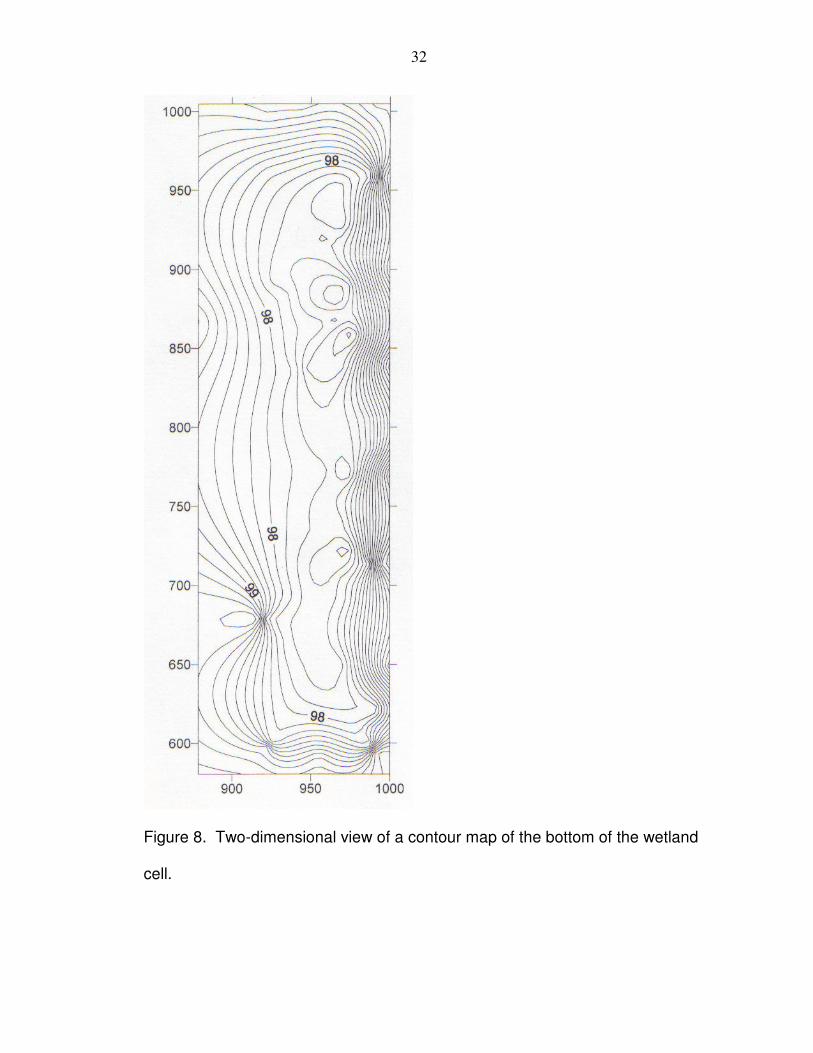
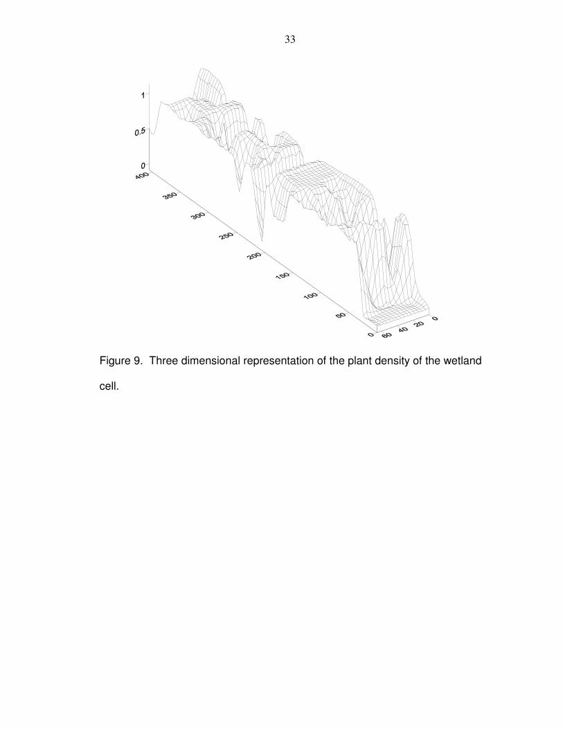
4.3 Bathymetry survey

In the next four figures, there are two three-dimensional maps and two

contour maps of the depth of the cell one and the plant density of cell one.

Figures 7 and 8 are survey maps of relative elevations, and because of the

sludge depth in the mixing zones, surveying points were only taken at the

corners of each wetland zone. Figures 9 and 10 are graphical representations of

a very basic plant density survey, where 1.0 means that grid was completely

vegetated, 0.5 means that the grid was half vegetated, and 0.0 means that the

grid was not vegetated at all. The grid for Figure 8 is also larger, in order to

encompass vegetation that is growing outside of the original wetland cell.

In order to orient the reader for Fig. 7 and 8, the side of the wetland cell

farthest of the x-axis is the side closest to the aeration ponds. It is also the side

from which the sampling points are measured.

In order to orient the reader for Fig. 9 and 10, the side of the wetland cell

closest to the x-axis is the side closest to the aeration pond. The density is done

in proportions. A density of 1.0 is has a density of 100%, and a densities of 0

and less are open water.

31

Figure 7. Three-dimensional view of the depth of the wetland cell.

32

Figure 8. Two-dimensional view of a contour map of the bottom of the wetland

cell.

33

Figure 9. Three dimensional representation of the plant density of the wetland

cell.

34

Figure 10. Two dimensional contour map of the plant density of the wetland cell.

35

5.0 Discussion and Conclusions

The tracer study had a very distinctive pattern. It is more like uniform flow

than a normalized or bell curve. For the purposes of this study, the graph will be

called a curve. The curve itself had three very distinctive peaks, with four smaller

ones. This suggests that the wetland cell is experiencing short-circuiting and

stagnation zones. The last peak and the tail of the curve further indicate this.

The mean hydraulic retention time is 7.7 days. Referring to Figure 6,

there is also a range of hydraulic retention times that appear to fall between 4.5

days to 17.8 days. The first peak indicates a short circuit that is faster than the

others, while the stagnation zones are indicated by the lingering tail of the curve.

Now, the hydraulic efficiency should be analyzed. According to Persson

et al. (1997), the hydraulic efficiency is calculated as mean hydraulic retention

time divided by the nominal hydraulic detention time, which gives means that λ is

equal to 0.497, or 0.50. This means that the wetland cell could be on the verge

of sliding into poor hydraulic efficiency, which is the characterized by a λ between

0.50 and 0.25.

Also, as stated in Persson (2000) λ equal to e that is a proportion that is

also equal to the effective volume divided by the design volume. This means that

the effective volume of the wetland cell for this experiment was approximately

601,000 gallons, or half of the design volume. From this, it can be concluded

that cell one is accumulating more sludge and plant matter than is allowed in the

36

design specifications. Once the sludge and plant debris is removed, the mean

hydraulic retention time should become longer and approach design hydraulic

retention time.

This conclusion is not as well supported by the mixing zone data. In two

out of the three cases possible in a paired t-test, the means of the dye

concentrations in and the dye concentrations out were found to be significantly

different (Table 8). However, based on the results of the analysis of variance

tests, it is the interaction between the positions, inlet and outlet side of the mixing

zone, and the distance from the side that the samples were taken that provides

the difference in dye concentrations that suggests mixing is still occurring in the

mixing zones.

From visual observations, it does appear as though the mixing zone is

filling with sludge. In addition, the higher mean at the fifteen feet distance also

indicates that more dye is reaching that point. It appears that the mixing zone

could still be providing homogeneity by acting as a stagnation zone. However,

there is still the preferential flow that is providing a 4.5 days hydraulic retention

time for part of the dye concentration.

Part of the answer may be found in the plant density data. Referring to

Figures 9 and 10, there are areas of open water. These areas may be providing

faster flow conditions when the information is combined with the information from

Figures 7 and 8. The survey maps suggest that the side nearest the aeration

pond, and nearest to the fifteen feet sampling points, has a steeper slope than

the other side. In other areas, the combination of fully vegetated and open water

37

areas may be producing stagnation zones, which the mixing zone data suggests

it has become.

In conclusion, the wetland cell should be monitored carefully. If the

hydraulic efficiency begins to decline, or the interaction between the inlet and

outlet side of the mixing zone and the distance from the side of the wetland cell

decreases, measures should be taken to remove the sludge buildup in the mixing

zones and replant the wetland cell.

38

6.0 References

Batchelor, Allan and Pierre Loots. 1997. "A critical evaluation of a pilot scale subsurface flow wetland: 10 years after commissioning." Water Science and Technology, 35(5), 337-343.

King, Andrew C., Cynthia A. Mitchell and Tony Howes. 1997. “Hydraulic tracer

studies in a pilot scale subsurface flow constructed wetland.” Water Science and Technology, 35(5), 189-196.

Hilton, Amy B., Drew L. McGillivary, and E. Eric Adams. 1998. “Residence time

of freshwater in Boston’s inner harbor. Journal of Waterway, Port, Coastal, and Ocean Engineering, 124(2), 82-89.

Kadlec, Robert H. 1994. "Detention and mixing in free water wetlands."

Ecological Engineering, 3, 345-380. Persson, J., N.L.G Someo, and T.H.F. Wong. 1999. "Hydraulic efficiency of

constructed wetlands and ponds." Water Science and Technology, 40(3), 291-300.

Persson, J. 2000. “The hydraulic performance of ponds of various layouts.”

Urban Water, 2(3), 243-250. Precision Planning, Inc. 1992. Excerpts from design report. Rash, Jonathan K. and Sarah K. Liehr. 1999. "Flow pattern analysis of

constructed wetlands treating landfill leachate." Water Science and Technology, 40(3), 309-315.

Schnabel, R.R., W.L. Stout, and J.A. Shaffer. 1995. "Uptake of a hydrologic

tracer (bromide) by ryegrass from well and poorly drained soils." Journal of Environmental Quality, 24, Sept.-Oct., 888-892.

Simi, Anne L., and Cynthia A. Mitchell. 1999. "Design and hydraulic

performance of a constructed wetland treating oil refinery wastewater." Water Science and Technology, 40(3), 301-307.

Werner, Timothy M. and Robert H. Kadlec. 2000. "Wetland residence time

distribution modeling." Ecological Engineering, 15, 77-90.

39

7.0 APPENDIX

7.1 Prototype Run

Mixing Zone Grab Samples

Table 9. Inlet Side of the Mixing Zone

Absorbance at 520 nm Date 15 ft 30 ft 45 ft

10/10/2001 -0.0137

-0.0044

0.0004

10/11/2001 -0.0059

0.0010 0.0234

10/12/2001 0.0057 0.0088 0.0075 10/13/2001 0.0110 -

0.0149 -

0.0063 10/15/2001 0.0692 0.0505 0.0163 10/16/2001 0.2940 0.0355 -

0.0011 10/17/2001 0.0293 0.0219 0.0250 10/18/2001 0.1247 0.0204 0.0122 10/19/2001 0.1263 0.0246 0.0110

Concentration, mg active indgredient/L

Date 15 ft 30 ft 45 ft 10/10/2001 N/D* N/D 0.1267 10/11/2001 N/D 0.1812 2.2177 10/12/2001 0.6085 0.8903 0.7722 10/13/2001 1.0903 N/D N/D 10/15/2001 6.3815 4.6814 1.5722 10/16/2001 26.8186** 3.3177 N/D 10/17/2001 2.7540 2.0813 2.3631 10/18/2001 11.4271** 1.9449 1.1994 10/19/2001 11.5726** 2.3268 1.0903

40

Table 10. Outlet Side of the Mixing Zone

Absorbance at 520 nm Date 15 ft 30 ft 45 ft

10/10/2001 -0.0145

-0.0075

-0.0056

10/11/2001 -0.0082

0.0132 -0.0069

10/12/2001 0.0140 0.0059 0.0036 10/13/2001 -

0.0100 -

0.0041 -

0.0089 10/15/2001 0.0173 0.0346 0.0120 10/16/2001 -

0.0037 -

0.0069 0.0035

10/17/2001 0.0222 0.0228 0.0197 10/18/2001 0.0151 0.0115 0.0091 10/19/2001 0.0055 0.0213 0.0158

Concentration, mg active indgredient/L

Date 15 ft 30 ft 45 ft 10/10/2001 N/D N/D N/D 10/11/2001 N/D 1.2904 N/D 10/12/2001 1.3631 0.6267 0.4176 10/13/2001 N/D N/D N/D 10/15/2001 1.6631 3.2359 1.1813 10/16/2001 N/D N/D 0.4085 10/17/2001 2.1086 2.1631 1.8813 10/18/2001 1.4631 1.1358 0.9176 10/19/2001 0.5903 2.0267 1.5267

41

Table 11. Outlet Zone Samples Over Time

Sample #

Date Absorbance at 520 nm

Concentration, mg of active ingredient/L

Hours

1 10/9/01 4:18 PM 0.0242 3.1032 0 2 10/9/01 6:18 PM 0.0166 2.4122 2 3 10/9/01 8:18 PM -0.0098 0.0122 4 4 10/9/01 10:18 PM -0.0258 N/D* 6 5 10/10/01 12:18 AM -0.0247 N/D 8 6 10/10/01 2:18 AM -0.0199 N/D 10 7 10/10/01 4:18 AM -0.0284 N/D 12 8 10/10/01 6:18 AM -0.0207 N/D 14 9 10/10/01 8:18 AM -0.0221 N/D 16

10 10/10/01 10:18 AM -0.0213 N/D 18 11 10/10/01 12:18 PM -0.0157 N/D 20 12 10/10/01 2:18 PM -0.0029 0.6395 22 13 10/10/01 4:18 PM 0.0105 1.8577 24 14 10/10/01 6:18 PM 0.0024 1.1213 26 15 10/10/01 8:18 PM 0.0034 1.2122 28 16 10/10/01 10:18 PM -0.0006 0.8486 30 17 10/11/01 12:18 AM -0.0045 0.4940 32 18 10/11/01 2:18 AM -0.0084 0.1394 34 19 10/11/01 4:18 AM -0.0141 N/D 36 20 10/11/01 6:18 AM -0.0121 N/D 38 21 10/11/01 8:18 AM -0.0124 N/D 40 22 10/11/01 10:18 AM -0.0003 0.8758 42 23 10/11/01 12:18 PM -0.0051 0.4394 44 24 10/11/01 2:18 PM 0.0061 1.4577 46 25 10/11/01 4:18 PM 0.0072 1.5577 48 26 10/11/01 6:18 PM 0.0169 2.4395 50 27 10/11/01 8:18 PM 0.0120 1.9941 52 28 10/11/01 10:18 PM 0.0144 2.2122 54 29 10/12/01 12:18 AM 0.0155 2.3122 56 30 10/12/01 2:18 AM 0.0064 1.4849 58 31 10/12/01 4:18 AM 0.0101 1.8213 60 32 10/12/01 6:18 AM 0.0132 2.1031 62 33 10/12/01 8:18 AM 0.0071 1.5486 64 34 10/12/01 10:18 AM 0.0120 1.9941 66 35 10/12/01 12:18 PM 0.0096 1.7759 68 36 10/12/01 2:18 PM 0.0186 2.5941 70 37 10/12/01 4:18 PM -0.0037 0.5667 72 38 10/12/01 6:18 PM 0.0052 1.3758 74 39 10/12/01 8:18 PM 0.0004 0.9395 76 40 10/12/01 10:18 PM -0.0049 0.4576 78

42

41 10/13/01 12:18 AM -0.0078 0.1940 80 42 10/13/01 2:18 AM -0.0026 0.6667 82 43 10/13/01 4:18 AM -0.0100 N/D 84 44 10/13/01 6:18 AM -0.0081 0.1667 86 45 10/13/01 8:18 AM -0.0079 0.1849 88 46 10/13/01 10:18 AM 0.0018 1.0667 90 47 10/13/01 12:18 PM 0.0099 1.8031 92 48 10/13/01 2:18 PM 0.0245 3.1305 94 49 10/13/01 4:18 PM 0.0171 2.4577 96 50 10/13/01 6:18 PM 0.0130 2.0850 98 51 10/13/01 8:18 PM 0.0132 2.1031 100 52 10/13/01 10:18 PM 0.0119 1.9850 102 53 10/14/01 12:18 AM 0.0139 2.1668 104 54 10/14/01 2:18 AM 0.0130 2.0850 106 55 10/14/01 4:18 AM 0.0161 2.3668 108 56 10/14/01 6:18 AM 0.0192 2.6486 110 57 10/14/01 8:18 AM 0.0236 3.0486 112 58 10/14/01 10:18 AM 0.0284 3.4850 114 59 10/14/01 12:18 PM 0.0150 2.2668 116 60 10/14/01 2:18 PM 0.0242 3.1032 118 61 10/14/01 4:18 PM 0.0178 2.5213 120 62 10/14/01 6:18 PM 0.0293 3.5668 122 63 10/14/01 8:18 PM 0.0177 2.5123 124 64 10/14/01 10:18 PM 0.0155 2.3122 126 65 10/15/01 12:18 AM 0.0128 2.0668 128 66 10/15/01 2:18 AM 0.0093 1.7486 130 67 10/15/01 4:18 AM 0.0086 1.6849 132 68 10/15/01 6:18 AM 0.0060 1.4486 134 69 10/15/01 8:18 AM 0.0049 1.3486 136 70 10/15/01 10:18 AM 0.0413 4.6578 138 71 10/15/01 12:18 PM 0.0267 3.3305 140 72 10/15/01 2:18 PM 0.0361 4.1850 142 73 10/15/01 4:18 PM 0.0377 4.3305 144 74 10/15/01 6:18 PM 0.0039 1.2577 146 75 10/15/01 8:18 PM -0.0059 0.3667 148 76 10/15/01 10:18 PM -0.0808 N/D 150 77 10/16/01 12:18 AM -0.0066 0.3031 152 78 10/16/01 2:18 AM -0.0051 0.4394 154 79 10/16/01 4:18 AM -0.0104 N/D 156 80 10/16/01 6:18 AM -0.0071 0.2576 158 81 10/16/01 8:18 AM -0.0093 0.0576 160 82 10/16/01 10:18 AM -0.0064 0.3213 162 83 10/16/01 12:18 PM 0.0010 0.9940 164 84 10/16/01 2:18 PM 0.0115 1.9486 166

43

85 10/16/01 4:18 PM 0.0104 1.8486 168 86 10/16/01 6:18 PM 0.0138 2.1577 170 87 10/16/01 8:18 PM 0.0140 2.1759 172 88 10/16/01 10:18 PM 0.0069 1.5304 174 89 10/17/01 12:18 AM 0.0056 1.4122 176 90 10/17/01 2:18 AM 0.0075 1.5849 178 91 10/17/01 4:18 AM 0.0028 1.1577 180 92 10/17/01 6:18 AM 0.0060 1.4486 182 93 10/17/01 8:18 AM 0.0072 1.5577 184 94 10/17/01 10:18 AM 0.0091 1.7304 186 95 10/17/01 12:18 PM 0.0120 1.9941 188 96 10/17/01 2:18 PM 0.0154 2.3032 190 97 10/17/01 4:18 PM 0.0132 2.1031 192 98 10/17/01 6:18 PM 0.0087 1.6940 194 99 10/17/01 8:18 PM 0.0059 1.4395 196

100 10/17/01 10:18 PM 0.0017 1.0577 198 101 10/18/01 12:18 AM 0.0075 1.5849 200 102 10/18/01 2:18 AM 0.0047 1.3304 202 103 10/18/01 4:18 AM 0.0057 1.4213 204 104 10/18/01 6:18 AM 0.0069 1.5304 206 105 10/18/01 8:18 AM 0.0094 1.7577 208 106 10/18/01 10:18 AM 0.0141 2.1850 210 107 10/18/01 12:18 PM 0.0314 3.7578 212 108 10/18/01 2:18 PM 0.0249 3.1668 214

N/D mean no dye detected.

7.2 Second Sampling Run

Calibrations Sets

44

Table 12. Calibration Set for Date: 2/22/02

Set 1 mg/L abs mg/L abs

0 0 0 0 0.2 0.0041 0.2 0.0041 0.4 0.0089 *** 0.6 0.0071 0.6 0.0071 0.8 0.0089 0.8 0.0089 1.0 0.0109 1.0 0.0109

Set 2

mg/L abs 0.0 0 2.0 0.0193 4.0 0.0456 6.0 0.0678 8.0 0.0703

10.0 0.0913

Set 3 mg/L abs

0.0 0 20.0 0.1861 40.0 0.3649 60.0 0.5145 80.0 0.6708

100.0 0.8732

Set 4 mg/L abs

0.0 0 200.0 1.8043 400.0 2.6331 600.0 2.7806 800.0 2.8729

1000.0 2.9613

45

Table 13. Calibration set for Date 2/26/02

Set 1 mg/L abs

0 0 0.2 0.0045 0.4 0.0059 0.6 0.0091 0.8 0.0144 1.0 0.239

Set 2 mg/L abs

0.0 0 2.0 0.0302 4.0 0.0451 6.0 0.0715 8.0 0.0824

10.0 0.0986

Table 14. Calibration set for Date 2/28/02

Set 1 mg/L abs mg/L abs

0 0 0 0 0.2 0.0013 0.2 0.0013 0.4 0.0045 0.4 0.0045 0.6 0.0201 *** 0.8 0.0121 0.8 0.0121 1.0 0.0107 1.0 0.0107

Set 2 mg/L abs

0.0 0 2.0 0.025 4.0 0.0337 6.0 0.0518 8.0 0.0695

10.0 0.0784

46

Table 15. Calibration set for Date 3/4/02

Set 1 mg/L abs

0 0 0.2 0.0025 0.4 0.008 0.6 0.0096 0.8 0.0114 1.0 0.0321

Set 2 mg/L abs

0.0 0 2.0 0.0322 4.0 0.0615 6.0 0.0872 8.0 0.1157

10.0 0.1496

Table 16. Calibration Set for Date 3/12/002

Set 1 mg/L abs mg/L abs

0 0 0 0 0.2 0.0012 0.2 0.0012 0.4 0.0035 0.4 0.0035 0.6 0.0104 *** 0.8 0.0083 0.8 0.0083 1.0 0.0159 1.0 0.0159

Set 2 mg/L abs

0.0 0 2.0 0.0453 4.0 0.0607 6.0 0.0715 8.0 0.104

10.0 0.1243 Inlet Mixing Zone Concentrations

47

Table 17. Inlet mixing zone concentrations for the experimental run

Date Absorbance Concentration, mg/l

2/18/2002 --- --- 2/19/2002 0.0106 0.923163927 2/20/2002 0.0185 1.611182325 2/21/2002 0.0129 1.123473081 2/22/2002 -0.0211 0 2/23/2002 -0.0113 0 2/24/2002 -0.0041 0 2/25/2002 0.0008 0.069672749 Aquarium Samples Table 18. Dye degradation samples A1

Date Absorbance Time ln (Abs/Abs0)

02/22/02 2.9341 1 -0.02221 02/26/02 3.0060 5 0.001998 02/28/02 3.0243 7 0.008067 03/08/02 2.9467 15 -0.01793 03/12/02 2.5970 19 -0.14426 A2

Date Absorbance Time ln (Abs/Abs0)

02/22/02 3.0909 1 0.02985 02/26/02 3.1690 5 0.054804 02/28/02 3.1546 7 0.050249 03/08/02 2.3290 15 -0.25317 03/12/02 0.9191 19 -1.18297 Where A1 refers to Aquarium 1, and A2 refers to Aquarium 2.