Theoretical modeling of x-ray and vibrational spectroscopies applied to liquid water and surface adsorbates By Mathias P. Ljungberg Doctorate Thesis in Chemical Physics at Stockholm University 2010
Transcript
Theoretical modeling of x-ray and
vibrational spectroscopies applied to liquid
water and surface adsorbates
By
Mathias P. Ljungberg
Doctorate Thesis in Chemical Physics at
Stockholm University 2010
2
Abstract
This thesis presents results of theoretical modeling of x-ray and vibrational spectroscopies appliedto liquid water and to CO adsorbed on a Ni(100) surface. The Reverse Monte Carlo method is usedto search for water structures that reproduce diffraction, IR/Raman and x-ray absorption by fittingthem to experimental data and imposed constraints. Some of the structures are created to havea large fraction of broken hydrogen bonds because recent x-ray absorption and emission studieshave been seen to support the existence of such structures. In the fitting procedure a fast wayof computing the IR/Raman spectrum for an isolated OH stretch is used, where the frequency isrepresented by the electric field projected in the direction of the stretch coordinate. This method iscritically evaluated by comparing it to quantum chemical cluster calculations. Furthermore, the x-ray emission spectrum of water is investigated, the modeling of which is complicated by the necessityof including vibrational effects in the spectrum calculations due to a dissociative intermediate state.Based on the Kramers-Heisenberg formula a new semi-classical method is developed to includevibrational effects in x-ray emission calculations. The method is seen to work very well for a one-dimensional test system. Moreover, x-ray absorption and emission are implemented in a periodicDensity Functional Theory code which is applied to ice and to the surface adsorbate system CO onNi(100).
This thesis is based on the following seven papers, which will be referred to by their correspondingroman numerals throughout this thesis.
I. Are recent water models obtained by fitting diffraction data consistentwith infrared/Raman and x-ray absorption spectra? M. Leetmaa, M.Ljungberg, H. Ogasawara, M. Odelius, L-A. Naslund, A. Nilsson and L.G.M.PetterssonJ. Chem. Phys., 125, 244510 (2006)
II. Diffraction and IR/Raman Data Do Not Prove Tetrahedral Water M.Leetmaa, K.T. Wikfeldt, M. P. Ljungberg, M. Odelius, J. Swenson, A. Nilssonand L.G.M. PetterssonJ. Chem. Phys., 129, 084502 (2008)
III. Assessing the electric-field approximation to IR and Raman spectraof dilute HOD in D2O M. P. Ljungberg, A. P. Lyubartsev, A. Nilsson andL.G.M. PetterssonJ. Chem. Phys. 131, 034501 (2009)
IV. Vibrational interference effects in x-ray emission for a system with adissociative intermediate state: the water dimer (Manuscript) M.P.Ljungberg, L.G.M. Pettersson and A. Nilsson
V. Semi-classical description of nuclear dynamics in x-ray emission of wa-ter (Manuscript) M.P. Ljungberg, A. Nilsson and L.G.M. Pettersson
VI. An implementation of core level spectroscopies in a real space Projec-tor Augmented Wave code (Manuscript) M. P. Ljungberg, J.J Mortensenand L.G.M. Pettersson
VII. Theoretical Approximations to X-ray Absorption Spectroscopy of Liq-uid Water and Ice M. Leetmaa, M. P. Ljungberg, A. Lyubartsev, A. Nilsson,and L. G. M. PetterssonJ. Electron Spec. Rel. Phen. 177, 135-157 (2010)
ii
i
Work not included in this thesis.
A. X-ray Spectroscopy Calculations within Kohn-Sham DFT: Theory andApplications (Book Chapter) Mikael Leetmaa, Mathias Ljungberg, AndersNilsson, and Lars Gunnar Moody Pettersson.In Computational methods in Catalysis and Materials Science, An introductionfor Scientists and Engineers, Edited by Rutger A. van Santen and PhilippeSautet, Wiley, (2009)
B. The inhomogeneous structure of water at ambient conditions C. Huang,K. T. Wikfeldt, T. Tokushima, D. Nordlund, Y. Harada, U. Bergmann, M.Niebuhr, T. M. Weiss, Y. Horikawa, M. Leetmaa, M. P. Ljungberg, O. Takahashi,A. Lenz, L. Ojamae, A. P. Lyubartsev, S. Shin, L. G. M. Pettersson, and A.Nilsson Proc. Natl. Acad. Sci. (USA) 106, 15214 (2009)
C. On the Range of Water Structure Models Compatible with X-ray andNeutron Diffraction Data Kjartan T. Wikfeldt, Mikael Leetmaa, Mathias P.Ljungberg, Anders Nilsson and Lars G. M. Pettersson J. Phys. Chem. B, 113,6246 (2009)
D. Complementarity between high-energy photoelectron and L-edge spec-troscopy for probing the electronic structure of 5d transition metalcatalysts Toyli Anniyev, Hirohito Ogasawara, Mathias P. Ljungberg, Kjar-tan T. Wikfeldt, Janay B. MacNaughton, Lars-Ake Naslund, Uwe Bergmann,Shirlaine Koh, Peter Strasser, Lars G. M. Pettersson and Anders NilssonPhysical Chemistry Chemical Physics, in press
E. Electronic structure calculations using GPAW: A real-space imple-mentation of the projector-augmented wave method J. Enkovaara, C. Ros-tgaard, J. J. Mortensen, J. Chen, M. Du lak, L. Ferrighi, J. Gavnholt, C. Glinsvad,H. A. Hansen, H. H. Kristoffersen, M. Kuisma, A. H. Larsen, L. Lehtovaara,M. Ljungberg, O. Lopez-Acevedo, P. G. Moses, J. Ojanen, T. Olsen, V. Pet-zold, N. A. Romero, J. Stausholm, M. Strange, G. Tritsaris, M. Vanin, M. Wal-ter, B. Hammer, H. Hakkinen, G. K. H. Madsen, R. M. Nieminen, J. Nørskov,M. Puska, T. Rantala, J. Schiøtz, K. S. Thygesen, K. W. JacobsenScientific highlight in Psi-k Newsletter, No 98, April 2010.http://www.psi-k.org/newsletters/News 98/Highlight 98.pdf
F. Reply to Soper et al.: Fluctuations in water around a bimodal dis-tribution of local hydrogen-bonded structural motifs C. Huang, K. T.Wikfeldt, T. Tokushima, D. Nordlund, Y. Harada, U. Bergmann, M. Niebuhr,T. M. Weiss, Y. Horikawa, M. Leetmaa, M. P. Ljungberg, O. Takahashi, A. Lenz,L. Ojamae, A. P. Lyubartsev, S. Shin, L. G. M. Pettersson, and A. NilssonProc. Natl. Acad. Sci. (USA), 107, E45 (2010)
A spectroscopic measurement is one of the most fundamental methods to probe matter. By mea-suring the interaction of the system of study with light or particles as a function of energy a lot ofinformation can be gained about, for example, the positions of the atoms, the electronic structure,or how the molecules vibrate and rotate. Different spectroscopies probe different properties andare thus complementary; each one gives a piece of information that can be combined to give a con-sistent picture. The last few decades theoretical modeling of spectra using computers has becomeincreasingly important, as the computers have grown more powerful and the theoretical methodsmore advanced. Today it is more rule than exception to support an interpretation of experimentaldata with theoretical modeling.
This thesis deals with theoretical modeling of spectroscopies: X-ray Absorption (XAS), X-rayEmission (XES) and IR/Raman -applied to liquid water and to CO on Ni(100). Water is one of themost important substances on Earth and without it life as we know it would be impossible. It is akey component in uncountable biological, geological and technical processes. The understanding ofthe microscopic structure of water is necessary to be able to model the chemistry that takes place inwater solution, which includes all of biochemistry and numerous applications in for example catalysisand fuel cells. Furthermore, water in itself presents a scientific challenge: though being a chemicallysimple substance it is not easily understood. In fact, water has many anomalies like a very highboiling point, a density maximum at 4 degrees C, an unusually high compressibility etc.[1] Theseanomalies can be traced back to the properties of the hydrogen bond (H-bond), which in strengthis between the covalent bond and the van der Waals interaction. The possibility of water moleculesto form between zero and four H-bonds allows many types of structures to be almost isoenergetic,leading to a complex phase diagram [1].
The standard picture of water, with continuous distortions around a basically tetrahedral ar-rangement of water molecules has been around for more than 60 years [2, 3]. It is supported byMolecular Dynamics (MD) simulations which first appeared in water research in the late 1960’s[4, 5] and are very popular today. All commonly used MD force fields, e.g. SPC/E and TIP4P, givestructures that correspond to the standard picture - this is also the case for ab initio simulationswhere the forces are calculated with Density Functional Theory (DFT). X-ray and neutron diffrac-tion have been reported to agree very well with MD-derived structures [6, 7] and the experimentalIR/Raman spectrum has been well reproduced [8, 9, 10, 11].
In 2004 Wernet et al. published an article in Science where the standard model of water wasquestioned based on XAS experiments combined with DFT calculations [12]. It was claimed that toagree with XAS, water must be much less coordinated than in the standard model, with an averagenumber of H-bonds per water molecule of around two instead of nearly four. Furthermore, theXES of water shows a split lone pair peak (1b1, the highest occupied molecular orbital in water)
3
4 CHAPTER 1. INTRODUCTION
which was interpreted in ref [13] as being due to two distinct structural motifs, where a minorityis ice-like and the majority is very H-bond distorted, supporting the low H-bond count suggestedby Wernet et al. These results have caused significant discussion and it has been claimed in severalpublications that the standard model could still explain XAS and XES [14, 15, 16, 17, 18, 19, 20]while other publications support Wernet et al. [13, 21]. On the other hand, any new water modelmust be critically evaluated in the light of the success of the MD-models. So, can a structure witha number of H-bonds of around two per molecule reproduce diffraction and IR/Raman data? Muchof the work in this thesis was done to find answers to these questions and to see what constraintsexperimental data actually put on the structure of liquid water. In the course of doing this wehad to do some method development: we implemented new data sets in a Reverse Monte Carlocode (used to build structures), we critically evaluated the so called E-field approximation to theIR/Raman spectrum and developed a more accurate method to compute it, we developed a semi-classical approximation to the Kramers-Heisenberg formula to include effects of nuclear dynamics inXES, and we implemented XAS and XES in a periodic DFT code. To test the latter implementationwe computed XAS and XES for CO on Ni(100) and XAS for ice. The first two chapters in thisthesis contain descriptions of the background theory of electronic structure and x-ray and vibrationalspectroscopies. Included in the second chapter are also some of the theoretical developments thatwe made use of in the papers. Chapter three is a summary of the main results of the seven papersthat this thesis is based on.
Chapter 2
Electronic structure calculations
Finding solutions to the Schrodinger equation for a many-particle system is a very difficult task.For one-body or simple two-body problems it is sometimes possible to obtain analytic solutions,examples include the hydrogen atom and the harmonic oscillator. However, already the 3-bodyproblem becomes too difficult to solve exactly and must instead be solved numerically. The many-body wave function for a system of n particles depends on the spatial coordinates of all n particlesΨ(r1, r2, r3..., rn) which means that the problem is 3n-dimensional. A brute force solution to thisproblem is clearly unfeasible for n larger than 2 or 3 which means that approximate methods haveto be found. For a molecular system the first step is to separate the electronic and nuclear degreesof freedom.
2.1 The Born-Oppenheimer approximation
Consider a quantum mechanical system, with Hamiltonian H0, in a given state at t = 0. Then applya perturbation f(t) ·H1 with the function f going slowly from 0 to 1. The adiabatic theorem statesthat if the perturbation is turned on slowly enough, the system will remain in the state it startedin. The wave function has ”time to adapt” to the changing potential and will at each moment intime be an eigenfunction of the instantaneous Hamiltonian. This requires that there is a continuousmapping between the states of the unperturbed and the perturbed system so that each state can beidentified, which is the case when the spacing between the states is large.
The most famous example of an adiabatic approximation is the Born-Oppenheimer (B-O) ap-proximation where the changing positions of the nuclei can be seen as a slow perturbation for theelectrons. The nuclei can be thought to move on an electronic Potential Energy Surface (PES), withthe electrons always being in an instantaneous eigenstate at the given nuclear configuration. For asystem of n electrons in a potential of N nuclei the Hamiltonian is (in atomic units):
H =∑
a
P 2a
2Ma+
∑
i
p2i
2mi+
∑
i<j
1
|ri − rj |−
∑
ia
Za
|ri − Ra|+
∑
a<b
ZaZb
|Ra − Rb|(2.1)
where the first two terms are the kinetic energy of the nuclei and the electrons, the other termsare Coulomb interactions among the electrons and nuclei. To simplify the notation we denote allelectronic coordinates by r and all nuclear coordinates by R; we write the Hamiltonian as
Tel + Tnuc + V (r,R) (2.2)
In the B-O approximation our ansatz for the total wave function is:
5
6 CHAPTER 2. ELECTRONIC STRUCTURE CALCULATIONS
Ψ(r,R) = ψ(r; R)χ(R) (2.3)
where χ(R) is the nuclear wave function and ψ(r; R) the electronic wave function that dependsparametrically on the nuclear coordinates R, i.e. solved with R fixed. For the electronic wavefunction we have the equation:
[Tel + V (r,R)]ψn(r; R) = ǫn(R)ψn(r; R) (2.4)
To determine χ(R) we put in ψn(r; R)χnm(R) in the total Schrodinger equation:
(
Tel + Tnuc + V (r,R))
ψn(r; R)χnm(R) = Enmψn(r; R)χnm(R) (2.5)
Since we already solved the electronic problem this equation reduces to:
(
ǫn(R) + Tnuc
)
ψn(R; r)χnm(R) = Enmψn(r; R)χnm(R) (2.6)
Now we make the approximation that ψn(r; R) is a constant with respect to the nuclear kineticenergy operator Tnuc, which makes it possible to remove ψn(r; R) from the equation, arriving at:
(
ǫn(R) + Tnuc
)
χnm(R) = Enmχnm(R) (2.7)
This equation can be interpreted as the nuclear wave function moving on a potential energy surfaceǫn(R) generated by the electronic wave function in its n:th state. To more clearly see the assumptionsof this approximation we apply the nuclear kinetic energy operator on ψ(r; R)χ(R) which gives:
−∑
a
1
2Ma∇2
Ra(ψ(r; R)χ(R)) =
= −∑
a
1
2Ma
(
ψ(r; R)∇2Rχ(R) + χ(R)∇2
Rψ(r; R) + 2∇Rψ(r; R) · ∇Rχ(R))
(2.8)
If the equation were fully separable then the last two terms would be zero. So the condition forthe B-O approximation to be valid is that the first and second derivatives ( 1
2Ma∇Rψ(r; R) and
12M ∇2
Rψ(r; R) ) of the electronic wave function with respect to the nuclear coordinates must be
small. Note the division by the nuclear mass which makes these terms smaller for heavy nuclei. Incertain cases the terms can be non-negligible, for example in the case of curve crossings where theB-O approximation breaks down and we get vibronic couplings. Assuming the B-O approximationis valid the electronic problem can be solved in the potential from stationary nuclei whose positionscan be varied to map out a Potential Energy Surface (PES). The Schrodinger equation can then besolved for the nuclei moving on this PES to obtain the vibrational wave functions.
In the opposite case, where the perturbation is turned on quickly, the wave function has no timeto adapt and it ends up as a superposition of eigenstates of the perturbed system. In the case of anelectronic transition, the vibrational wave function ends up in a superposition of eigenstates of theexcited state PES which can be seen in the spectrum as a distribution of peaks, each corresponding toa vibrational eigenstate. This can be explained using the Franck-Condon (FC) picture (see section3.1.2). Also for core excitations the frequency of excitation can be so high that the remainingelectrons don’t have time to respond, and satellite peaks show up in the spectrum correspondingto additional electronic excitations. In the case of core excitations this is usually called the suddenapproximation (which is equivalent to the FC picture). Even for purely vibrational transitions theFC picture can be applicable if one mode can be considered fast compared to the others.
These two extremes, the adiabatic and the sudden limits, are extensively used and can greatlysimplify many problems.
2.2. HARTREE-FOCK THEORY 7
2.2 Hartree-Fock Theory
The simplest ansatz to solving the electronic problem is to assume that the problem is separable,which means that our wave function can be written as a product of one-particle wave functions:Ψ(r1, r2, r3..., rn) = ψ1(r1)ψ2(r2)...ψn(rn), this is called a Hartree product. If the n particles areidentical they will obey either boson or fermion statistics depending on their spin; the wavefunctionmust be symmetric resp. antisymmetric with respect to interchange of particle coordinates. Elec-trons are fermions and should have antisymmetric wave functions with respect to interchange ofparticle coordinates; such a wave function can be constructed as a determinant of the one-particlewave functions
Ψ(r1, r2, r3..., rn) =1√N !
∣
∣
∣
∣
∣
∣
∣
ψ1(r1) ψ2(r1) . . .
ψ1(r2) ψ2(r2) . . ....
.... . .
∣
∣
∣
∣
∣
∣
∣
(2.9)
A wave function like this is called a Slater determinant and it is the simplest many-particle wavefunction that obeys Fermi statistics. This is the form of the wave function in the Hartree-Fockapproximation. Let us now concentrate on the electronic problem. The energy is 〈ψ|H |ψ〉 and fora Slater determinant this becomes
E = −1
2
∑
i
∫
ψ∗i (r1)∇2
iψi(r1)dr1 +1
2
∑
ij
∫ |ψi(r1)|2|ψj(r2)|2|r1 − r2|
dr1dr2
−1
2
∑
ij
∫
ψ∗i (r1)ψ∗
j (r2)ψi(r2)ψj(r1)
|r1 − r2|dr1dr2 −
∑
ia
Za
∫ |ψi(r1)|2|Ra − ri|
dr1 +1
2
∑
a6=b
ZaZb
|Ra − Rb|(2.10)
where the first term is the kinetic energy, the second is the Coulomb interaction between the elec-trons, the third is the exchange term which is purely quantum mechanical and cannot be interpretedin a classical way. The last two terms are Coulomb interactions between the electrons and nuclei,and nuclei-nuclei. The different terms are a consequence of the determinantal wave function withorthogonal orbitals, for one-electron operators only diagonal terms give rise to a non-zero contribu-tion, for two-electron operators only diagonal and terms with two orbitals switched contribute. Ifthe energy expression is minimized with respect to the orbitals the Hartree-Fock equations result[22, 23]:
Fψi = ǫiψi (2.11)
where F is called the Fock operator,
Fψi(r1) =
−1
2∇2 −
∑
a
Za
r − Ra+
∑
j
∫ |ψj(r2)|2|r1 − r2|
dr2
ψi(r1) −∑
j
∫
ψ∗j (r2)ψi(r2)
|r1 − r2|dr2ψj(r1)
(2.12)These equations must be solved self-consistently. The Hartree-Fock method gives by constructionthe best single-determinantal wave function that satisfies fermionic statistics, but more complicatedwave functions can be constructed. The most straightforward way of improving on Hartree-Fock isConfiguration Interaction (CI). The CI wave function is a linear combination of several determinants,using the orbitals obtained from, e.g., a Hartree-Fock calculation. Another possibility to improve theHartree-Fock method is by perturbation theory. The Møller-Plesset perturbation theory methods,especially the second-order one called MP2, is commonly employed. The state of the art method
8 CHAPTER 2. ELECTRONIC STRUCTURE CALCULATIONS
(at least for small molecules) is the Coupled Cluster method. This method can be seen as a CImethod which implicitly includes higher excitations due to an exponentially parameterized excitationoperator. The ”Golden standard” CCSD(T) coupled cluster method with singles and doubles andperturbative triples gives very good accuracy and is often used as a benchmark method. A summaryof these post-Hartreee-Fock methods can be found in [22]. Although accurate, these methods arequite expensive to use; Hartree-Fock scales formally as N4, MP2 as N5 and CCSD(T) as N7 withthe number of basis functions. For large systems it becomes very expensive to use a correlated wavefunction method and an alternative is to use Density Functional Theory (DFT) which sometimescan give better results than MP2 at a lower computational cost.
2.3 Density Functional Theory (DFT)
In DFT one deals with the electron density instead of the wave function as the basic quantity thatcharacterizes the system. The wave function depends on the spatial coordinates of all particleswhich means that its complexity is strongly dependent on the number of particles. The density onlydepends on three space variables no matter how many the particles are and this makes it a muchsimpler quantity. The basic theorems of DFT were published in two seminal papers: the first in 1964by Hohenberg and Kohn [24], and the second a year later by Kohn and Sham [25]. In the first paperit was shown that the external potential (the potential from the nuclei) is uniquely determined bythe ground state electron density (except for an additive constant). Since the number of electronsis the integrated electron density the Hamiltonian is determined, which in turn determines thewave function. This can be seen the following way: the positions of the nuclei are determined bycusps in the electron density and the derivatives of the electron density at the cusp give the nuclearcharges (the Kato cusp condition). Together with the total number of electrons this determines theHamiltonian [26]. Also, an energy functional of the density was defined and a variational principlewas established which means that the energy functional is minimized for the ground state density.Unfortunately the functional is unknown and must be approximated.
In the second paper Kohn and Sham invent a trick to approximate the kinetic part of theenergy: to partition it into the kinetic energy of a non-interacting system and a remaining correction.The non-interacting system is described by a Slater determinant of one-particle orbitals that areconstructed to give the same density as the interacting system. The non-interacting kinetic energycan be calculated from the orbitals and this will make up the major part of the interacting kineticenergy. The Kohn-Sham energy functional is:
E[ρ] = −1
2
∑
i
∫
ψ∗i (r)∇2
iψi(r)dr +
∫
ρ(r)ρ(r′)
|r − r′| drdr′ −
∑
a
Za
∫
ρ(r)
|r − Ra|dr + Exc[ρ] (2.13)
where Exc is the exchange correlation functional, that is the correction term that includes everythingthat is not Coulomb energy or the non-interacting kinetic energy. In Kohn-Sham DFT the orbitalsserve as the new basic variables instead of the density. Minimizing eq 2.13 with respect to theorbitals will also minimize it with respect to the density since ρ(r) =
∑
i |ψi(r)|2. Constrainingthe orbitals to be orthogonal and performing the minimization results in the Kohn-Sham (K-S)equations:
(
−1
2∇2 + veff (r)
)
ψi(r) = ǫiψi(r) (2.14)
veff =
∫
ρ(r′)
|r − r′|dr′ + vxc(r) −
∑
a
Za
|r − Ra|(2.15)
2.4. LCAO CODES 9
with
vxc(r) =δExc[ρ]
δρ(r)(2.16)
The only difference between the Hartree-Fock equations and the Kohn-Sham equations is that theexchange term is replaced by the exchange correlation potential vxc. These equations are solved self-consistently. The formal scaling of these equations can be reduced to N3 because the density can betreated as a single variable that can be expanded in a basis set, this procedure is called density fitting.Alternatively, one can solve the Poisson equation for the Hartree potential (first term in eq 2.15)numerically which is done in most periodic codes. Since the true exchange-correlation functional isunknown an approximate one must be constructed and this can be done in several different ways.A guiding principle is that the functional should reproduce some limiting cases exactly, the mostimportant one is that of the interacting homogeneous electron gas. For this system the exchangeenergy can be calculated analytically while the correlation energy can be calculated with highprecision using Quantum Monte Carlo methods [27]. A functional parametrized to the interactingelectron gas is called Local Density Approximation (LDA) or Local Spin Density Approximation(LSDA) for the spin-polarized case [28, 29]. The LDA functional works well for many solids butnot for molecules since in the latter case the electron density is rapidly varying and not very similarto the electron gas. Improvements to the LDA scheme can be made, the most straight-forwardone is the Generalized Gradient Approximation (GGA), where also information about the densitygradient is incorporated in the functional [30, 31]. With GGA:s molecules can be better described.Hybrid functionals mix in a part of Hartree-Fock exchange into the functional and this leads toimproved results for molecules. One of the most used hybrid functionals is B3LYP [32, 33], whichis an empirical mix of LDA, GGA, and Hartree-Fock exchange.
2.4 LCAO codes
The implementations of DFT can be roughly categorized as being either non-periodic or periodic.Most non-periodic codes use the LCAO (Linear Combination of Atomic Orbitals) method where abasis set of atom-centered basis functions is used to expand the molecular orbitals. For practicalreasons almost all LCAO codes have used Gaussians as basis set; the advantage is that most of thenecessary matrix elements can be calculated analytically. Lately numerical basis sets have grownpopular [34, 35] because such a basis set allows more flexibility -a basis function can for example beforced to be zero outside a certain radius, which makes the overlap and other matrices sparse. InLCAO codes a molecular orbital is expanded in atom-centered basis functions:
ψi(r) =∑
a
cai φj(r − ra) (2.17)
Taking matrix elements of the Fock operator in this basis we end up with
Fc = ScE (2.18)
with Snm = 〈φn|φm〉, the basis function overlap matrix, c the vector of expansion coefficients andE a diagonal matrix of eigenvalues. The H-F (or K-S) equations turn into a generalized matrixeigenvalue problem called the Roothan-Hall equations in the H-F case.In the case of DFT the matrix elements of the Kohn-Sham potential are computed numerically dueto the complicated form of the potential. The eigenvalue problem can be solved by standard linearalgebra routines, like those included in the LAPACK library [36]. Examples of LCAO codes includeGaussian, StoBe, Demon2k, Siesta. Recently LCAO basis sets have been implemented in the GPAWcode [37].
10 CHAPTER 2. ELECTRONIC STRUCTURE CALCULATIONS
2.5 Periodic codes
For a periodic system with a least repeating unit cell, A, the wave function can be written as a partperiodic in A times a phase, this is Bloch’s theorem [38]
ψnk(r) = unk(r)eik·r (2.19)
The density is ρ(r) =∑
n
∫
BZ dk|unk(r)|2 [39] where the sum is over all occupied orbitals, that isorbitals with energy lower than the Fermi level, and the k variable is integrated over the first BrillouinZone. In practice the k variable must be sampled which turns the integral into a sum. The K-Sequations for different k-points separate and have to be combined only at the end when the densityis updated. Doubling the cell is equivalent to doubling the number of k-points effectively sampled-thus it is possible to only sample the BZ at k=(0,0,0) (the Gamma point) if a sufficiently largecell is used. However, the computational effort will increase much faster for a larger cell comparedto using k-points; this is because the number of basis functions and orbitals are proportional tothe number of atoms and the scaling is more than linear with respect to those parameters whilebeing linear in the number of k-points. The number of k-points that one has to use depends on thedispersion of the bands - for a large dispersion many k-points have to be used.
In many metals the valence electrons can be considered to be almost free since the core electronsefficiently screen the nuclear attraction. This fact makes it natural to use plane waves as basisfunctions, and the whole problem can be recast in momentum space. A problem with a plane wavesbasis set is that a very large basis set is required to describe the region near the nuclei where theorbitals are rapidly varying - to come to terms with this problem a smooth pseudopotential canbe used instead of the real potential. The pseudopotential gives smoother valence wave functions(the core states are frozen and not explicitly treated). Even with a pseudopotential the basis setis large enough so that a direct diagonalization of the Fock matrix is impractical, instead only acertain number of states is determined using iterative methods. The plane wave pseudopotentialmethod is efficient for systems with a small unit cell since k-point sampling is much more efficientthan using a larger supercell and furthermore the number of k-points can often be greatly reducedbecause of symmetry. Some popular plane wave pseudopotential codes include VASP, PWSCF,ABINIT, daCapo. However, for systems with large unit cells, needed to compute for examplesurface adsorbates in a low coverage phase, one cannot use the advantages of the k-point samplingand the basis set becomes so large that the calculation has to be parallelized to finish in a resonabletime. Recently therefore there has been interest in real space basis sets for which parallelization oflarge systems is straightforward [34].
2.5.1 The Projector Augmented Wave (PAW) method
In the PAW method [40, 34] a linear mapping is constructed between the all-electron wave functionsψn(r) and the pseudo wave functions ψn(r).
ψn(r) = T ψn(r) (2.20)
The mapping T is
T = 1 +∑
a
∑
i
(|φai 〉 − |φa
i 〉)〈pai | (2.21)
where the pseudo wave function is corrected by adding and subtracting terms centered at theatoms. The all-electron partial waves, |φa
i 〉, are basis functions suitable to describe the true valencewave function within some radius around the atom, the pseudo partial waves, |φa
i 〉 are suitablefor describing the pseudo wave function in the same region, and |pa
i 〉 are projector functions. The
2.6. THE VIBRATIONAL PROBLEM 11
mapping thus projects away the pseudo wave function in the atomic region and adds the true one.The atom-centered functions are constructed from an atomic calculation and usually it is enough touse two functions per angular momentum (in the GPAW code the pre-computed atomic functions,along with potentials and densities are stored in an object referred to as a ”setup”). The totalenergy expression can be rewritten using this transformation and a Hamiltonian can be derived byminimizing the total energy with respect to the pseudo density [40].
H|ψn〉 = ǫnS|ψn〉, (2.22)
The Hamiltonian is similar to the Fock operator of the full problem, however, since the number ofbasis functions is huge a direct conversion of the problem into a matrix equation is not feasible andit is instead solved using iterative methods, like RMM-DIIS [34]. The PAW method is consideredto be an improvement of the pseudopotential method since all corrections to the expressions usingpseudo wave functions can be computed, which in principle leads to all-electron accuracy (althoughwith frozen core states).
GPAW is a DFT code that implements the PAW method [37]. It is predominantly written inPython with only the most time-consuming parts written in C. The wave functions and density arerepresented on a real-space grid and finite difference and multigrid methods are used to solve theKohn-Sham equations. Both periodic and non-periodic boundary conditions can be imposed. Thisscheme allows for efficient parallelization where domain-decomposition as well as parallelization overspins, k-points and bands is used. Fairly large systems with a few hundred atoms and cell sizes ofaround 20x20x20 A can be studied routinely. Recent developments in the code include LCAO basissets, x-ray absorption spectroscopy, Time-Dependent Density Functional Theory (TDDFT) [41].The implementation of x-ray absorption spectroscopy in the GPAW code is described in section(3.1) and furthermore in paper VI.
2.6 The vibrational problem
A molecular system of n atoms has 3n degrees of freedom since each atom can move in the x, y andz directions. If the system is free to move as a whole, which is the case for a gas phase cluster butnot for a surface where usually some degrees of freedom are frozen, the translations of the center ofmass have three degrees of freedom and the rotations another three - except for linear systems whichhave two rotations. The remaining 3n -6 (3n -5) degrees of freedom are the vibrational modes.
Assuming the B-O approximation to be valid the geometry of the system can be optimized bysearching for a minimum of the PES - this can be done with for example the quasi-Newton methodwhich requires calculating the forces on the nuclei. To proceed to solve the nuclear Schrodingerequation the PES is then expanded in a Taylor series in the Cartesian displacements of the nucleiaround the minimum. Since the geometry is optimized the force is zero, so the first non-vanishingterms in the expansion are of second order. If only the second order terms are retained (the socalled harmonic approximation) the solution of the vibrational problem is much simplified since it ispossible to find a linear transformation that decouples the vibrational modes. The new coordinatesthat result from the linear transformation are called Normal coordinates.
2.6.1 Normal coordinates
Define a vector x of Cartesian displacements of the atoms, ordered as (∆x1,∆y1,∆z1,∆x2,∆y2,∆z2,. . . ,∆xn,∆yn,∆zn). The classical kinetic energy is
T =1
2
∑
i
mi(xi)2 (2.23)
12 CHAPTER 2. ELECTRONIC STRUCTURE CALCULATIONS
The potential energy is expanded in a Taylor series around the minimum
V (x1, x2, ..., xn) = V0 +∑
i
(
∂V
∂xi
)
xi +∑
ij
(
∂2V
∂xi∂xj
)
xixj + . . . (2.24)
where the linear term is zero at the equilibrium geometry. V0 is arbitrary and can be set to zero.So we have to second order:
V =∑
fijxixj (2.25)
where fij = ∂2V∂xi∂xj
. To simplify the expressions for T and V we introduce mass-weighted coordinates,
qi =√mixi getting
T =1
2
∑
i
(qi)2 (2.26)
V =∑
ij
cijqiqj (2.27)
where now cij =∑
ij1√
mimj
∂2V∂xi∂xj
. The Lagrange equations are, with L = T−V , ∂L∂qi
− ddt
(
∂L∂qi
)
= 0.
We thus have the equations:
qi +∑
j
cijqj = 0 (2.28)
which is a set of coupled differential equations. However, it is possible to find an orthogonal trans-formation of the coordinates so that neither the kinetic nor the potential energy has any cross terms.This is done by diagonalizing the matrix c:
∑
kl
tikckltlj = ω2i δij (2.29)
With this transformation the kinetic energy becomes: T = 12
∑
i Q2i and the potential energy:
V =∑
ij
qicijqj =∑
ijklmn
qitik(tklclmtmn)tnjqj =∑
i
ω2iQ
2i (2.30)
where Qi =∑
k qktki are the normal coordinates and ωi are the frequencies of vibration. This canbe seen from the Lagrange equations which now read
Qi + ω2iQi = 0 (2.31)
and have solutions Qi(t) = e±iωit which means that ωi are the vibrational frequencies. One can gofrom the classical expressions in the normal coordinates of T and V to the corresponding quantummechanical expressions. This can be done naively by treating the normal coordinates as Cartesiancoordinates, or in a more rigorous way [42]. Both give the same result and the quantum mechanicalHamiltonian becomes:
H = T + V =∑
i
p2i +
∑
i
ω2iQ
2i (2.32)
The normal coordinates thus allow us to decouple a coupled system, provided that the potentialenergy is truncated at second order. They are the best vibrational coordinates for small displace-ments around equilibrium where the potential energy surface can be approximated by a quadratic
2.6. THE VIBRATIONAL PROBLEM 13
polynomial. For large displacements normal coordinates can be a bad choice; they are linear combi-nations of Cartesian displacements so all atoms must move in straight lines. This can lead to largecouplings, especially for floppy modes. Being comparably rigid the OH stretch mode in the watermolecule should be well approximated by the corresponding normal mode. For cluster models ofliquid water different clusters have slightly different normal modes, which could lead to an effectiveinclusion of couplings compared to an internal stretch approach. When using normal coordinatesthe issue of reduced mass becomes unambiguous since it follows from the definition of the normalmode. The reduced masses are calculated as mk = 1
||Qk||2 where Qk are the usual normal modes.
This can be seen by noting that the normal coordinates are not normalized to one, they are in factscaled with some reduced mass, so if one wants to use normalized Cartesian displacements insteadone has to use the correct reduced mass. In the normal mode calculation six (five) frequencies willbe zero (or close to it, depending on the accuracy of the calculation): they are the three translationsof the center of mass and the three (two) rotations of the whole system which must be handledseparately. For our purposes we ignore them.
14 CHAPTER 2. ELECTRONIC STRUCTURE CALCULATIONS
Chapter 3
X-ray and vibrationalspectroscopies
In a one-particle picture x-ray absorption (XAS) can be viewed as exciting a core electron to anunoccupied orbital. When the incoming x-ray has sufficient energy to excite a core electron from acertain shell there is a sharp rise in the absorption cross section; this is called an absorption edge.The edges are named depending on the shell of the core electron: K-edge refers to the excitation of a1s electron, L-edge to 2s or 2p electrons, M-edge to 3s, 3p, 3d electrons and so on. Experimentally, itis favorable to measure the highest angular momentum for a certain value of the principal quantumnumber. The features near the edge contain a lot of information about the local surroundings ofthe atoms since one probes the local density of states, albeit in the presence of a core hole. Thestudy of the near-edge region is called NEXAFS (Near Edge X-ray Absorption Fine Structure) orXANES (X-ray Absorption Near Edge Structure). Above the edge the cross section will decayexponentially but there is still information in the oscillations of the cross section, which are usedin EXAFS (Extended X-ray Absorption Fine Structure). EXAFS can be most easily understoodin terms of multiple-scattering: the scattered electron bounces back from neighboring atoms andcreates standing waves for certain energies, which give rise to the oscillations in the absorption crosssection. EXAFS is mostly used to get information about the coordination of the atoms. Here wewill instead focus on the NEXAFS region.
When the core electron has been excited a core hole remains, and it decays in a few femtosecondsby an electron falling down to occupy the core level, leaving the system with a hole in the valence.The excess energy released by the decay process can induce the ejection of another electron (Augerdecay), thus leaving the system with two valence holes, or the emission of a photon, and this latterprocess is called X-ray emission (XES). Auger decay is difficult to interpret due to the two valenceholes, but XES can be interpreted in a simple orbital picture. Simplified, one can say that XASprobes the unoccupied orbitals and XES the occupied ones.
3.1 X-ray absorption spectroscopy (XAS)
XAS is described with Fermi’s Golden Rule (here as in the rest of the chapter we set h to 1):
σ(ω) ∝∑
f
|〈Ψf |D|Ψi〉|2 δ(ω − Efi) (3.1)
where Ψf and Ψi denote final and initial many body-states and D = E ·r is the dipole operator withE the polarization direction of the incoming photon. The delta function ensures energy conservation
15
16 CHAPTER 3. X-RAY AND VIBRATIONAL SPECTROSCOPIES
and gives peaks when the frequency is equal to the energy differences of the states. In reality theexcited states have a finite lifetime which means that the energy has an uncertainty in accordancewith Heisenberg’s uncertainty principle. The delta function is then replaced by a Lorentzian functionwith a broadening parameter Γ which is the half width at half maximum (HWHM) of the peak.
δ(Efi − ω) → 4Γ
(Efi − ω)2 + Γ2(3.2)
In a one-electron picture, describing all excitations as singly-excited determinants using the groundstate orbitals, eq 3.1 becomes
σ(ω) ∝∑
f
|〈ψf |D|ψi〉|2 δ(ω − ǫfi) (3.3)
where now ψf and ψi denote the unoccupied and core orbitals respectively and ǫfi is the differencebetween their eigenvalues. For a 1s core hole (K-edge), the selection rules of the dipole operator givesnonzero contributions for orbitals with p character, thus probing the unoccupied p density of states.However, the independent particle picture neglects the important relaxation effects from the creationof the core hole. If the ground state and the excited states can be optimized separately eq 3.1 can beused, with the caveat that the states now are many-body wave functions. For molecules it is possibleto separately optimize several core-excited states at the Hartree-Fock level by imposing a certainsymmetry of the wave function [43], and the excitation energies are thus obtained as total energydifferences between the ground state and the selected core-excited state. Determining excitationenergies this way is called Delta SCF. It has been successfully used with DFT as well (see paper VII),which makes it possible to also include correlation effects in the calculation. One must remember,however, that the K-S wave functions are solutions to an auxiliary non-interacting problem andwill only reproduce the density of the true wave function. This means that an excited state ingeneral cannot rigorously be optimized by forcing orbital occupations or orthogonality between K-Sdeterminants. In practice, Delta SCF energies computed with DFT agree better with experimentthan the ones computed with Hartree-Fock [44]. To distinguish the DFT case from the HF casewe call it Delta Kohn-Sham (DKS) in the following. There are rigorous theories for separatelyoptimized states within time-independent DFT which justify the DKS procedure [45, 46, 47]. Inthose theories however the Exchange-correlation functional should be state-dependent, and it is ofcourse unknown. DKS with a regular ground state functional can nevertheless be regarded as anapproximation in these theories.
It is in principle possible to compute higher core-excited states by forcing them to be orthogonalto the lower ones. In the StoBe code this is done by setting up the Kohn-Sham matrix in a basisof molecular orbitals and simply deleting all off diagonal matrix elements for one orbital, whichmeans that it cannot change during the SCF optimization. The occupation for this orbital is setto zero and the diagonalization gives a new set of occupied orbitals that is orthogonal to it. If adeterminant has one orbital that is orthogonal to every orbital in a second determinant the twodeterminants are orthogonal. In practice, one can choose to delete the off-diagonal elements of theHOMO of the first core excited state, and delete the new HOMO of the second one to get the third,and so on, and this has been done for small molecules [48]. For large systems where the density ofstates is high this would be unfeasible. We therefore have to use some more approximate method toget the excited states, like the Transition Potential (TP) method [49] (see also paper VII). The TPmethod is an approximation to the Slater transition state [50], which in turn is an approximationto DKS. In Slater’s transition state the transition energy between the ground state and a separatelyoptimized excited state with a hole in a certain orbital is approximated with the orbital energydifferences in a state with the orbitals involved half occupied. The transition state is in a way ”halfway between” the ground state and the excited state, if one allows a fraction of the electron to be
3.1. X-RAY ABSORPTION SPECTROSCOPY (XAS) 17
moved from an orbital to another, and it has been shown to be correct to second order [50]. Inpaper VII we repeat the derivation by Slater. This scheme only requires one calculation insteadof a separate ground state and excited state calculation, but a separate calculation is required foreach excited state. A further approximation is to ignore the excited electron, which leads to thehalf-core-hole (HCH) or Transition-Potential (TP) method, which then reduces the problem to anindependent-particle problem in the half core hole potential. Other core hole potentials that arecommonly used are the full core hole (FCH) where a full electron is removed from the core orbitaland the excited core hole (XCH) where a full electron has been removed from the core orbital andinserted in the lowest unoccupied orbital. In papers V and VII the different core hole potentials arecompared and discussed for diamond and ice K-edge XAS.
In the TP-DFT method the intensities are computed from the one-particle orbitals, which mustbe seen as an additional approximation since the DKS and Slater’s transition state are used fortransition energies, not intensities. In the StoBe code, which is an all-electron code, we optimize thecore excited state by setting the occupation of the relevant alpha spin 1s orbital to zero, putting anextra electron in the first unoccupied alpha orbital and relaxing the wave function. If there is morethan one atom of the element that is core excited, the other atomic cores are described with EffectiveCore Potentials (ECP:s) to facilitate the identification of the core orbital to be excited. Also, if thesystem is spin polarized, the excitation of an alpha and a beta electron will give different spectra andshould be computed separately. To compute the spectrum with the TP-DFT method the density isfirst optimized with a half core hole, then the Kohn-Sham matrix is diagonalized using a very largeand diffuse basis set to be able to better represent continuum states. The size of this second basisset will determine the density of states in the the continuum region, as is discussed thoroughly inpaper VII. In the GPAW code we construct a special PAW setup with a core hole on the relevantsite and there is no need for a double basis set procedure since the grid basis already describes thecontinuum region well. DKS is well defined for the first core excited state and a comparison to DKSobtained with the deMon2k code can be found in paper VI. Vibrational effects in XAS can be takeninto account by the Franck-Condon approximation, section 3.1.2
3.1.1 Implementation of XAS in the GPAW code
Using the PAW transformation 2.21 we can rewrite the XAS cross section
〈ψi|D|ψf 〉 = 〈ψi|DT |ψf 〉 = 〈ψi|D
1 +∑
a
∑
j
(|φaj 〉 − |φa
j 〉)〈paj |
|ψf 〉
= 〈ψi|D|ψf 〉 +∑
a
∑
j
〈ψi|D|φaj 〉〈pa
j |ψf 〉 −∑
a
∑
j
〈ψi|D|φaj 〉〈pa
j |ψf 〉 (3.4)
The core state is localized and D is a local operator, which reduces the sum over atomic centers toa single term. Assuming that the pseudo partial waves form a complete set inside the augmentationsphere, that is
∑
a
∑
j |φaj 〉〈pa
j | = 1, the third term in eq 3.4 cancels with the first and we get
σ(ω) ∝∑
f
|〈ψf |φa〉|2δ(ω − Efi) (3.5)
with|φa〉 =
∑
j
|paj 〉〈φa
j |D|ψi〉 (3.6)
In eq 3.5 a lot of unoccupied states must be determined which is computationally demanding sincethe grid basis set is too large for an explicit diagonalization of the Kohn-Sham matrix. However, we
18 CHAPTER 3. X-RAY AND VIBRATIONAL SPECTROSCOPIES
can avoid determining the unoccupied states by using the Haydock recursion scheme [51, 52]. Thecross section can be rewritten as
σ(ω − Ei) ∝ − 1
πIm〈φa|S−1/2G(ω)S−1/2|φa〉 (3.7)
with the Green’s function
G(ω) =(
ω − S−1/2 ˜HS1/2 + iΓ
)
=∑
f
|ψf 〉〈ψf |ω − Ef + iΓ
=∑
f
S1/2|ψf 〉〈ψf |S1/2
ω − Ef + iΓ(3.8)
The overlap operator S comes in because the pseudo wave functions satisfy the orthogonality relation〈ψn|S|ψm〉 = δij . The pseudo wave functions are solutions to the effective Schrodinger equation
H |ψ〉 = ǫS1/2ψ〉 (3.9)
which can be transformed into a regular eigenvalue problem
S−1/2HS1/2|ψ〉 = ǫS1/2|ψ〉 (3.10)
which is the eigenvalue problem for the all-electron wave functions since |ψ〉 = T |ψ〉 = S1/2|ψ〉. TheGreen’s function of eq. 3.10 is given by 3.8.
In eq. 3.7 the absolute energy scale is lost because core eigenvalues are not implemented in the GPAWcode. Although this is possible, we can determine the absolute energy scale for the first transitionmore accurately with the DKS method, where the total energy of the final state is calculated usinga full core hole setup and an extra electron in the valence.
Now the cross section can be obtained by the Haydock recursion method, which is a way to findthe diagonal matrix element of the Green’s function by setting up a new orthogonal basis in whichS−1/2HS1/2 is tridiagonal using the Lanczos scheme. The recurrence relations become (see paperVI)
where the |wn〉 functions are normalized as 〈wn|S−1|wm〉 = δnm and bn is a normalization constant.The initial |wn〉 is taken as the normalized |φa〉. When the coefiicients an and bn have been computed,the whole spectrum up to an arbitray energy can be calculated without much work using thecontinued fraction expression:
〈φa|S−1/2G(ω)S−1/2|φa〉 =1
a0 − ω − iΓ − b21
a1−ω−iΓ− b22
...
(3.12)
These expressions involve the inverse overlap operator S−1 which is computed by solving the equationSx = y with the conjugate gradient method, or by employing an approximate inverse overlapoperator. In paper VI it can be seen that the approximate inverse is a good approximation for theXAS of diamond; perfect agreement is obtained if a few (e.g. 100) coefficients are computed exactlyand the rest approximately.
3.1. X-RAY ABSORPTION SPECTROSCOPY (XAS) 19
3.1.2 The Franck-Condon approximation
In the Franck-Condon (FC) picture an excitation of the electronic state induces transitions of thevibrational states. In chapter 2 it was mentioned that the FC picture is also applicable for secondaryelectronic excitations upon core excitation, and even sometimes in purely vibrational transitions.We call the fast degrees of freedom ”electronic” and the slow ”vibrational” although both might beeither electronic or vibrational depending on the situation. The transition energy will be the sum ofthe energies for the electronic and the vibrational transitions and the cross-section is proportionalto the square of the dipole matrix element. Indexing the electronic state in upper case and thevibrational state in lower case with fF representing vibrational state f belonging to the electronicstate F and using that the total dipole operator is the sum of the dipole operators for the electronicand nuclear coordinates, D = Dr +DR we have:
〈iI |〈I|D|F 〉|fF 〉 =
∫ ∫
ψ∗I (r; R)χ∗
Ii(R)(Dr +DR)ψF (r; R)χfF(R)drdR
=
∫ [∫
ψ∗I (r; R)DrψF (r; R)dr
]
χ∗Ii(R)χfF
(R)dR
+
∫[
∫
ψ∗I (r; R)ψF (r; R)dr
]
χ∗Ii(R)DRχfF
(R)dR (3.13)
The second term gives rise to vibrational transitions, but no electronic transitions since ψ∗I (r; R)
and ψF (r; R) are orthogonal. The transition energies for this term thus only depend on the energydifference of the vibrational levels and do not contribute at frequencies near transitions of theelectronic levels. So we are left with:
∫ [ ∫
ψ∗I (r; R)DrψF (r; R)dr
]
χ∗Ii(R)χfF
(R)dR = 〈iI |DIF |fF 〉 (3.14)
where the matrix element of the dipole operator is over the electronic coordinates - it is still anoperator in the nuclear coordinates:
DIF (R) =
∫
ψ∗I (r; R)DrψF (r; R)dr (3.15)
Starting in a given electronic and vibrational state we will get the exact (within the B-O approxi-mation) cross section as (skipping constants):
σ(ω) =∑
F,f
|〈iI |DIF |fF 〉|2δ(ω − EfF ,Ii) (3.16)
that is, the integral over the initial and final vibrational states weighted with the transition dipolesof the electronic states as a function of R. Neglecting the R-dependence of DIF (R) (the Condonapproximation) we can separate the two integrals, the transition is then described as a dipoletransition between electronic states multiplied with a monopole transition for the vibrational states.
σ(ω) =∑
F,f
|DIF |2|〈iI |fF 〉|2δ(ω − EfF ,iI) (3.17)
The overlap integrals for the vibrational states |〈iI |fF 〉|2 are called Franck-Condon factors. Invibrational spectrosopy, including the case of water, the Condon approximation is not valid forIR transitions (it is, however, for Raman transitions). A special case is when the ground state ofthe vibrational mode is bound and the excited state a continuum state. We can approximate thecontinuum state as a delta function, δ(R − R0), which gives
20 CHAPTER 3. X-RAY AND VIBRATIONAL SPECTROSCOPIES
〈iI |DIF |fF 〉 =
∫
χ∗Ii(R)DIF (R)δ(R − R0)dR = DIF (R)χ∗
Ii(R) (3.18)
This means that the spectrum will be a weighted average of electronic transitions, where the weightfunction is the initial vibrational wave function squared at coordinate R. Summing over all contin-uum states we get
σ(ω) =∑
F
∫
dR|DIF |2|χIi(R)|2δ(ω − (EF (R) − EIi) (3.19)
In a fully classical picture this reduces to
σ(ω) =∑
F
∫
dR|DIF |2 · p(R)δ(ω − (EF (R) − EI(R)) (3.20)
with p(R) the classical probability of the nuclei to be at point R. This means that one can samplethe ground state geometries from, e.g. , an MD simulation and average the spectra together toget the line shape. This corresponds to a classical Franck-Condon picture where all transitions arevertical - it can also be called the Vertical approximation (VA). This is also called the inhomogeneouslimit. In our XAS calculations of liquid water we assume the VA to hold, so that we should be ableto reproduce the vibrational profile of the spectra given a correct distribution of structures whosespectra are averaged. It seems, however, that at least the quantum distribution of the protons isimportant as can be seen in the comparison between spectra computed for the centroid and beadgeometries obtained from a path integral simulation (see paper VII). Eq 3.19 was used in paperVII to compute the vibrational line profile of the XAS spectrum of a water monomer. The groundstate vibrational wave function was obtained by first doing a normal mode analysis of the monomer,then the PES in the three normal coordinates was fitted to a polynomial of total degree 15 with amaximum degree of 10 in any of the three coordinates. A basis of harmonic oscillator functions wasused to variationally determine the vibrational eigenstates. The VA should be a good approximationfor a dissociative state but a bad approximation if the excited state vibrational eigenstates are wellseparated in energy.
In the opposite case, where the lifetime broadening is large in comparison to the envelope ofthe energy of excited vibrational states with an appreciable FC amplitude, we can consider theLorentzian broadening function to be centered at a mean transition energy ǫfi, which can be assumedto be the weighted average 1
N
∑
f ǫfi|〈iI |DIF |fF 〉|2. We can then expand the square and use theresolution of the identity to remove the sum over final states:
The lineshape is Lorentzian in this case and this is called the homogeneous limit. For x-ray emission(XES) the vibrational effects are more complicated since there are intermediate states that needto be taken into account which furthermore interfere during the lifetime of the excited state. Thisvibrational interference can have a large impact on the shape of the spectrum, especially if theintermediate electronic state is dissociative.
3.2. X-RAY EMISSION (XES) 21
3.2 X-ray Emission (XES)
XES generally has a dependence on the excitation energy as well as on interference effects involvingthe intermediate electronic and vibrational states. A rigorous way of taking these effects into acountis through the Kramers-Heisenberg formula:
σ(ω, ω′) =∑
f
∣
∣
∣
∣
∣
∑
n
〈f |D′|n〉〈n|D|i〉ω′ − En,f + iΓ
∣
∣
∣
∣
∣
2
Φ(ω − ω′ − Ef,0) (3.24)
with ω, ω′ and D, D’ being the energy and dipole operator of the incoming photon (unprimed) andthe emitted photon (primed). En,f = En − Ef is the energy difference between the intermediateand final states and Φ an instrumental function. In the case when an electron is excited to thecontinuum the dependence of the energy of the incoming photon disappears. In this case we writethe wave function as |n〉 = |n′〉|ǫn〉 and |f〉 = |f ′〉|ǫf 〉 where the primed wave functions denote theremaining bound state and |ǫ〉 is the wave function of the outgoing electron, labeled by its energy.Energies become En = En′ + ǫn and Ef = Ef ′ + ǫf , sums over states become
The transition dipole operator can be written as D = DN−1 +Dpe where the first part comes fromthe N-1 electrons in the remaining ion and the second from the photoelectron. Using this we canseparate the transition dipole matrix element as:
〈ǫf |〈f ′|D′N−1 +Dpe|n′〉|ǫn〉 = 〈ǫf |ǫn〉〈f ′|D′
N−1|n′〉 + 〈ǫf |Dpe|ǫn〉〈f ′|n′〉
≈ δ(ǫf − ǫn)〈f ′|D′N−1|n′〉 (3.26)
where in the last step we assume that only the first term contributes, that is that there are notransitions for the photoelectron. The integral over ǫn picks out the value of the integrand whereǫf = ǫn due to the delta function. This gives:
σ(ω, ω′) =∑
f ′
∫
dǫf
∣
∣
∣
∣
∣
∑
n′
〈f ′|D′N−1|n′〉〈ǫf |〈n′|D|i〉ω′ − En′,f ′ + iΓ
∣
∣
∣
∣
∣
2
Φ(ω − ω′ − Ef ′,0 − ǫf ) (3.27)
If we assume that the transition dipole matrix element between initial and intermediate states isindependent of ǫf the whole expression is independent of ǫf . The integral is then just over thebroadening function which gives a constant, one if it is normalized. In the following we do not writeout the wave function of the photoelectron or the primed ion states, assuming implicitly that thetransition dipole between intermediate and final states is between the states of the remaining ion andthat the photoelectron should be included in the matrix element between initial and intermediatestates (the last one, however, is often assumed to be a constant). We then end up with the expressionfor the non-resonant cross section, which now is independent of ω:
σ(ω′) =∑
f
∣
∣
∣
∣
∣
∑
n
〈f |D′|n〉〈n|D|i〉ω′ − En,f + iΓ
∣
∣
∣
∣
∣
2
(3.28)
22 CHAPTER 3. X-RAY AND VIBRATIONAL SPECTROSCOPIES
If we disregard the vibrational states we only have one intermediate state in this case and we canwrite
σ(ω′) =∑
f
|〈f |D′|n〉|2|〈n|D|i〉|2(ω′ − En,f )2 + Γ2
(3.29)
where the cross section is the product of an XAS transition and a transition from the intermediatestate (with a core hole) to the final states with a valence hole. For ionization the XAS cross sectionis approximately constant and we get the Fermi’s Golden Rule expression for XES
σ(ω′) ∝∑
f
|〈f |D′|n〉|2(ω′ − En,f )2 + Γ2
(3.30)
However, when considering vibrational effects or when doing resonant excitations equations 3.29and 3.30 can be a bad approximation and we have to use the expressions3.24 and 3.28.
To take vibrational effects into account for the non-resonant case we separate the electronic degreesof freedom from the vibrational ones so that we later can treat the latter in an approximate way. Wetake matrix elements over the electronic degrees of freedom, keeping the vibrational wave functions.The electronic matrix elements will still be operators in the vibrational coordinates.
σ(ω′) =∑
F
∑
fF
∣
∣
∣
∣
∣
∑
nN
〈fF |D′FN |nN 〉〈nN |DNI |iI〉ω′ − EnN ,fF
+ iΓ
∣
∣
∣
∣
∣
2
(3.31)
with nN representing vibrational state n belonging to the electronic state N .
3.2.1 Vibrational interference in the Kramers-Heisenberg formula
Since the sum over intermediate vibrational states is under the square sign we have cross terms inaddition to the diagonal ones. Under certain conditions the latter will dominate, however. Thedirect terms (just moving the sum out of the square and neglecting the cross terms) are [53]
∑
F
∑
fF
∑
nN
|〈fF |DFN |nN〉|2|〈nN |D′NI |iI〉|2
(ω′ − (EnN− EfF
))2 + Γ2(3.32)
while the interference terms are
∑
F
∑
fF
∑
nN
∑
mN 6=nN
〈fF |DFN |nN 〉〈nN |D′NI |0I〉
ω′ − (EnN− EfF
) + iΓ× 〈iI |D′
0N |mN 〉〈mN |DNF |fF 〉ω′ − (EmN
− EfF) − iΓ
(3.33)
If the denominator of this expression is large then each term will be small. The denominator is
1
ω′ − (EnN− EfF
) + iΓ× 1
ω′ − (EmN− EfF
) − iΓ
=1
(ω′ − (EnN− EfF
)) (ω′ − (EmN− EfF
)) + Γ2 − iΓ(EmN− EnN
)(3.34)
The sum over nN and mN runs over the same indices so there will be a pairing of terms with differentsign of the imaginary part in the denominator and the result is real (the numerator is also real).
3.2. X-RAY EMISSION (XES) 23
∑
F
∑
fF
∑
nN
∑
mN <nN
2〈fF |DFN |nN 〉〈nN |D′NI |iI〉 × 〈iI |D′
IN |mN 〉〈mN |DNF |fF 〉
× (ω′ − (EnN− EfF
))(ω′ − (EmN− EfF
)) + Γ2
[(ω′ − (EnN− EfF
))(ω′ − (EmN− EfF
)) + Γ2]2 + Γ2(EmN− EnN
)2(3.35)
If the term Γ2(EmN−EnN
)2 ≫ Γ4 it will dominate and make all terms small. This is equivalent tothe condition
∣
∣
∣
∣
EmN− EnN
Γ
∣
∣
∣
∣
≫ 1 (3.36)
The spacing between vibrational levels in the intermediate state is then much larger than the broad-ening Γ and the interference contributions can be neglected. This means that the spectrum is givenby the direct terms, which constitutes a two-step process without any interference between inter-mediate vibrational states. In the opposite case, when the lifetime broadening is much larger thanthe spacing between the intermediate states that have a considerable weight in the expansion of theinitial state, the energy of the individual intermediate states are not resolved so we can approximatethem with a single broad lorentzian centered at the mean energy, EnN
=∑
n c2nEnN
, with cn theexpansion coefficients of the ground state vibrational wave function in terms of the intermediatestates. We can then use the resolution of the identity to remove the sum over n and obtain:
σ(ω′) =∑
F
∑
fF
|〈fF |DFND′NI |iI〉|2
(ω′ − (EnN− EfF
))2 + Γ2(3.37)
A way to view this is that without interference the transitions between intermediate states and finalstates are well resolved and the intermediate states can be fully delocalized. This might then lead tocontributions to the spectra that correspond to dissociated products as well as the intact molecule,if the intermediate PES is dissociative. For the case of the water dimer model system in paper IVthe intermediate PES looks more or less like a square well as the potential will rise steeply when thedissociated hydrogen gets close to the accepting oxygen. Furthermore, all intermediate vibrationalstates that contribute to the FC profile when going from the ground state to the intermediate stateare delocalized; this is also the case for the lone pair (1b1) PES. This means that even in the limitof no interference, no assignment of peaks coming from intact or dissociates products can be made.
If the interference effects dominate, the transitions take place directly between the initial andfinal states which means that no delocalized intermediate states enter in the equation. This willlead to a different spectral shape that in the case of the water dimer in paper IV is narrowerand higher in energy than the case with no interference. However, since the final states are stilldelocalized in this case, the final vibrational wave function will always end up being delocalized.In this case the extra peaks to lower emission energy seen in the spectrum without interferencecannot be directly associated with dissociation, but must instead be seen to be the effect of lackof interference. Interference effects can also be seen in the time domain, where a large broadeningmeans a short lifetime. The excited wave packet thus has little time to move on the intermediatePES before it decays to the final state [54].
3.2.2 The Kramers-Heisenberg formula in the time domain
When using the KH formula in the energy domain the vibrational eigenfunctions of initial, interme-diate and final states must be calculated. This means that the PES’s of each state must be computedand the nuclear Schrodinger equation solved. For large systems with many degrees of freedom this
24 CHAPTER 3. X-RAY AND VIBRATIONAL SPECTROSCOPIES
is not feasible, and it is more advantageous to rewrite the KH formula in the time domain. We usethe following relations
1
2πi
∫ ∞
−∞dE
1
E − En + iΓe−iEt = θ(t)e−iEnt−Γt (3.38)
1
E − En + iΓ= −i
∫ ∞
−∞dtθ(t)e−iEnt−ΓteiEt = −i
∫ ∞
0
dte−iEnt−ΓteiEt (3.39)
where θ(t) is the Heaviside function. This leads to
σ(ω′) =∑
F
∑
fF
∣
∣
∣
∣
∣
−i∫ ∞
0
dt∑
nN
〈fF |DFN |nN 〉〈nN |D′NI |iI〉e−iEnN ,fF
t−Γteiω′t
∣
∣
∣
∣
∣
2
(3.40)
By using e−iEnNt|nN 〉 = e−iHN t|nN 〉 and 〈fF |eiEF t = 〈fF |eiHF t, where HN = 〈N |H |N〉 is the
Hamiltonian of the B-O PES of the electronic state N (and similarly for HF ), we have
σ(ω′) =∑
F
∑
fF
∣
∣
∣
∣
∣
−i∫ ∞
0
dt∑
nN
〈fF eiHF |DFNe
−iHN |nN 〉〈nN |D′NI |iI〉eΓteiω′t
∣
∣
∣
∣
∣
2
(3.41)
Expanding the square and using the resolution of the identity∑
i |i〉〈i| = 1 to remove the sums overintermediate states we get:
∑
F
∫ ∞
0
∫ ∞
0
dtdt′〈iI |D′INe
iHN tDNF e−iHF t · eiHF t′DFNe
−iHN t′D′IN |iI〉e−Γ(t+t′)eω′(t−t′) (3.42)
which can be written as
σ(ω′) =∑
F
〈iI |D†F (ω′)DF (ω′)|iI〉 = Tr(
∑
F
D†F (ω′)DF (ω′)ρ) (3.43)
with
DF (ω′) =
∫ ∞
0
dteiHF tDFNe−iHN tD′
INe−Γte−ω′t (3.44)
and ρ the density matrix of the system. From this expression a semi-classical approximation to theKH formula can be derived.
3.2.3 Semi-classical approximation to the Kramers-Heisenberg formula
Starting from the last expression we can make a semiclassical approximation that turns out to workvery well for a one-dimensional test system where the full KH cross-section can be computed, seepaper V. To be able to calculate the time development of the operators D we use the following [55]
e−iHF t = e−iHN te−i
R
t
0(HF (τ)−HN (τ))dτ
+ (3.45)
eiHF t = ei
R
t
0(HF (τ)−HN (τ))dτ
− eiHN t (3.46)
The exponentials with plus and minus signs are positive and negative time-ordered exponentials,[55]respectively which are defined as (for a Hermitian operator A)
3.2. X-RAY EMISSION (XES) 25
ei
R
t
0A(τ)dτ
− = 1 +
∞∑
n=1
in∫ t
0
dτn
∫ τn
0
dτn−1 . . .
∫ τ2
0
dτ1A(τ1)A(τ2) . . . A(τn) (3.47)
e−i
R
t
0A(τ)dτ
+ = 1 +∞∑
n=1
(−i)n
∫ t
0
dτn
∫ τn
0
dτn−1 . . .
∫ τ2
0
dτ1A(τn)A(τ2) . . . A(τ1) (3.48)
The Hamiltonian operators are written in the interaction representation
HF (τ) −HN (τ) = eiHN τ (HF −HN )e−iHN τ (3.49)
Here everything moves on the HN potential (the intermediate PES) and we can rewrite everythingin the interaction representation
DF (ω′) =
∫ ∞
0
dtei
R
t
0(HF (τ)−HN (τ))dτ
− eiHN tDFNe−iHN tD′
INe−Γte−ω′t (3.50)
=
∫ ∞
0
dtei
R
t
0(HF (τ)−HN(τ))dτ
− DFN(t) ·D′IN (0)e−Γte−ω′t (3.51)
So far everything is exact. We now make the semi-classical approximation: the time evolution istreated classically and the trace goes to a sum over classical trajectories on the intermediate PES,started from some ground state distribution. The time-ordered exponential becomes an ordinaryexponential with instantaneous intermediate and final state energies instead of the Hamiltonians,which finally gives us
σ(ω′) ∝ 1
N
∑
ntraj
∑
F
|DclassF (ω′)|2 (3.52)
DclassF (ω′) =
∫ ∞
0
dteiR
t
0(EF (τ)−EN(τ))dτDFN (t) ·D′
IN(0)e−Γte−ω′t (3.53)
These two equations are the final expressions for the SCKH cross section. This approximation isused in paper V and very good agreement to KH is obtained for a one-dimensional dissociative testsystem consisting of a water dimer with only the H-bonded hydrogen allowed to move.
3.2.4 Other approximations to the KH formula for non-resonant XES
Vibrational effects have been recognized to be of importance for the interpretation of XES of water[18, 13, 19, 20]. The vertical approximation (VA) can be used in XES as in XAS if both intermediateand final state vibrational wave functions are approximated as δ-functions. As in the XAS case wethen have to sum spectra according to the ground state probability distribution |χ0(R)|2.
σ(ω′) =∑
F
∫
dR|DFN (R)|2|D′
NI(E)|2|χ0(R)|2(ω′ − (EN (R) − EF (R)))2 + Γ2
(3.54)
This formula cannot include dissociative effects since only the ground state distribution is sampled.The approximation that has been used in [13, 19, 20] to include dynamical effects in the XESspectrum is an intuitive picture that similary to a configurational average for XAS spectroscopydoes the same for XES, with the difference that the spectra are averaged over classical trajectoriesrun on the intermediate state and weighted by an exponentially decreasing lifetime factor e−t/τ .The formula can be written as:
26 CHAPTER 3. X-RAY AND VIBRATIONAL SPECTROSCOPIES
σtraj(ω′,R(ti)) ≈∑
F
|DFN (R(ti))|2(ω′ − (EN (R(ti)) − EF (R(ti))))2 + Γ2
σtot(ω′) ≈
∑
traj
∑
i
σtraj(ω′,R(ti))e−ti/τ (3.55)
This formula is called Spectra Summed over Classical Trajectories (SSCT) in paper V. Since partof the controversy regarding the spectra calculations was about quantum initial conditions for theclassical trajectories on the core excited states, one can compare the SSCT to a similar expressionbut where the dynamics is performed quantum mechanically; this gives the Spectra Summed overWave Packet Probability (SSWPP) formula:
σ(ω′) ≈∑
F
∑
i
∑
j
|DFN (Rj)|2|χN (Rj , ti)|2e−ti/2τ
(ω′ − (EN (Rj) − EF (Rj)))2 + Γ2(3.56)
In paper V it is shown that SSCT with quantum initial conditions reproduced the SSWPP spectrumvery closely. However, both fail to reproduce the KH spectrum which on the other hand is wellreproduced by the SCKH method.
3.2.5 The lifetime of the intermediate electronic state
The lifetime broadening Γ is defined in this thesis, and in paper V as the Half Width at HalfMaximum (HWHM) of the Lorentzian function. Often however, Γ is defined as the Full Width atHalf Maximum (FWHM) which has created some confusion. The Fourier transform of the Lorentzianfunction with HWHM Γ is:
1
2π
∫ ∞
−∞
4Γ
(hω)2 + Γ=
1
he−
Γ
h |t| (3.57)
So if the lifetime τ is defined as usual like e−t/τ we see that τ = hΓ . In experimental publications
where the lifetime broadening has been measured, Γ has often been taken as the FWHM [56]. Usingthe formula τ = h
Γ with this gamma results in a lifetime that is a factor 2 too small. The reported
lifetime of 3.6 fs, should therefore be adjusted to 7.2 fs if the usual exponential decay e−t/τ is to beused.
3.3 IR and Raman spectroscopies
The vibrational and rotational motions of molecules give rise to transitions (absorption and emis-sion) in the infrared region of the spectrum. For a small molecule the rotational transitions havefrequencies of around 250 cm−1 [42] while the vibrational transitions occur in (approximately) therange 200-3750 cm−1. An absorption IR spectrum is obtained by passing infrared light throughthe sample and onto the spectrometer. The frequency of the light is scanned to pick out a certainvibrational transition.
In Raman spectroscopy one shines a monochromatic beam in the visible or UV region onto thesample and measures the light scattered from it. Most of the light will be elastically scatteredand will thus have the same frequency as the incoming light. However, some of the light will beinelastically scattered, leaving (or taking up) energy to excite (de-excite) a vibrational mode. For agiven vibrational level there will thus be two additional lines in the spectrum: one at lower frequencycorresponding to excitation of a vibrational mode and one at higher frequency corresponding to a
3.3. IR AND RAMAN SPECTROSCOPIES 27
de-excitation. These lines are called the Stokes and the Anti-Stokes lines respectively. By varyingthe polarization and the angles between the incoming and the measured light a lot of informationcan be obtained [42]. IR and Raman spectroscopies are complementary to each other because theyhave different selection rules. An IR transition is allowed for modes in which the dipole momentchanges during the vibration, for Raman the same is true for the polarizability. In gas phase onecan often observe quite sharp vibrational transitions that often are split because of couplings tothe rotational modes. In the condensed phase rotations and translations turn into broad bands ofcollective modes, and coupling to these modes broaden the vibrational bands substantially.
Hydrogen stretch modes are very high in frequency (3667 and 3756 in H2O for the symmetricand asymmetric stretch, respectively). For HOD the OH stretch is at 3707 and the OD stretch at2727 cm−1 [57]. Bend modes are lower, 1595 cm−1 in H2O and 1402 cm−1 in HOD [57]. In papersI,II and III the OH stretch mode of HOD in D2O is modeled, both for IR and Raman transitions.
3.3.1 IR and Raman intensities
In the dipole approximation the cross section for an IR transition is described by Fermi’s GoldenRule [58]
σ(ω) ∝∑
f
|〈i|E · µ|f〉|2δ(ω − Efi) (3.58)
where µ is the R-dependent total dipole moment of the system.
µ = 〈i|〈I|∑
j
rj −∑
k
ZkRk|I〉|f〉 = 〈i|〈I|∑
j
rj |I〉 −∑
k
ZkRk|f〉 (3.59)
Averaging over all orientations means summing the spectrum contributions from all three Cartesianpolarization vectors. For Raman we can get a similar expression
σ(∆ω) ∝∑
f
|〈i|α|f〉|2δ(∆ω − Efi) (3.60)
where α is the isotropic polarizability (for isotropic Raman ) [59, 60, 61]
α =1
3(αxx + αyy + αzz) (3.61)
with x,y,x denoting the spatial directions of the polarization of the incoming or emitted light. Eq.3.60 is an approximation to the KH formula. With the initial and final electronic states the same, andassuming that the lifetime of the intermediate state is short enough so that interference dominates,the resonant KH formula reads:
σ(ω, ω′) =∑
f
∣
∣
∣
∣
∣
∑
N
〈fI |D′INDNI |iI〉
ω − (EnN− EfF
) + iΓ
∣
∣
∣
∣
∣
2
δ(ω′ − ω − EfI+ EIi
) (3.62)
Setting ∆ω = ω′ − ω and using the argument of the δ-function to write the denominator as∆ω + ω − (EnN
− EiI) + iΓ we have
σ(ω, ω′) =∑
f
∣
∣
∣
∣
∣
∑
N
〈fI |D′INDNI |iI〉
∆ω + ω − (EnN− EiI
) + iΓ
∣
∣
∣
∣
∣
2
δ(∆ω − EfI+ EiI
) (3.63)
If ∆ω is small we can neglect it and the expression in the middle turns into the frequency dependentelectronic polarizability:
28 CHAPTER 3. X-RAY AND VIBRATIONAL SPECTROSCOPIES
αab(ω) =∑
N
D′INDNI
ω − (EnN− EiI
) + iΓ(3.64)
where a and b are the polarization of the incoming and emitted photon respectively. The frequencydependent polarizability can be approximated as the static polarizability, and formula 3.60 follows.We need to compute integrals of the type 〈i|α|f〉 and 〈i|µa|f〉 between the vibrational ground andexcited states. To this end we expand µa and α in the (assumed one-dimensional) vibrationalcoordinate R:
µa = µa(0) +
(
∂µa
∂R
)
R=0
R+ . . . (3.65)
α = α(0) +
(
∂α
∂R
)
R=0
R+ . . . (3.66)
so that our integral becomes (to first order)
〈i|µa|f〉 =
(
∂µa
∂R
)
R=0
〈i|R|f〉 (3.67)
〈i|α|f〉 =
(
∂α
∂R
)
R=0
〈i|R|f〉 (3.68)
The derivatives can be computed by calculating the relevant property at two or more points alongthe stretch coordinate and fitting a straight line through them. It is of course possible to compute thetransition matrix elements more accurately if we have more points along the vibrational coordinate.It is particularly easy to compute them in a DVR basis (section 3.3.2) and this was done in paper Vfor the dipole transitions. In paper III the linear Taylor expansion was used because the most time-consuming part was the calculation of the polarizability and limiting it to two points was deemednecessary.
3.3.2 Solving the 1-D vibrational problem
To reduce the cost of the vibrational problem the internal OH-stretch in HOD can be considered astotally uncoupled to the other modes. Neglecting all other vibrations gives a pseudo-diatomic withthe oxygen and deuterium atom together forming the other pseudo-atom. The one-dimensionalproblem can be solved by scanning the one-dimensional potential energy surface and solving theSchrodinger equation with the proper reduced mass for the system: mred = mA∗mB
mA+mB. Alternatively
normal coordinates can be used.
The Discrete Variable Representation (DVR) method
A DVR consists of a set of basis functions ui and a corresponding set of points xi [62]. The functionsui are localized at the corresponding point and are exactly zero on the other DVR points
ui(xj) = δi,j (3.69)
Any function can be expanded in the DVR basis
Ψk(x) ≃∑
i
ckiui (3.70)
3.3. IR AND RAMAN SPECTROSCOPIES 29
DVR:s are useful because the matrix element of a variable depending on x is approximated to bediagonal in the DVR basis
〈ui|V (x)|uj〉 ≃ V (xi)δi,j (3.71)
In fact, the points xi are chosen in such a way that the approximation of the integral by a sum is thebest possible. If the basis functions are orthogonal polynomials with respect to a weight function won the interval [a, b]
∫ b
a
pi(x)pj(x)w(x)dx = δi,j (3.72)
then the points xi are the Gaussian quadrature points on the interval. The weight function ismost easily included in the basis functions: χi(x) =
√
w(x)pi(x) which makes the basis functionsorthogonal with w = 1. To construct a DVR one only needs a set of orthonormal basis functionsχn. One sets up the matrix of the coordinate x in this basis 〈χn|x|χm〉 and diagonalizes it - theeigenvalues will be the DVR points xi and the eigenvectors the expansion coefficient for the DVRui expressed in the original basis χn
ui(x) =∑
n
T†inχn (3.73)
In matrix form (following [62]), where T † is the matrix whose columns are eigenvectors of X andXDV R is a diagonal matrix of the DVR points, that is XDV R
ij = δijxi this becomes
TXT † = XDV R (3.74)
The Hamiltonian is:
H = Hkin + V (x) (3.75)
The first way to set up the DVR Hamiltonian is to calculate the matrix elements of the kineticenergy analytically in the starting basis χn, then transform this matrix to the DVR basis by thetransformation T †
HDV Rkin = THkinT
† (3.76)
In the DVR basis the potential energy matrix is diagonal so the total DVR Hamiltonian becomes
HDV Ri,j = (THkinT
†)i,j + V (xi)δi,j (3.77)
The second way to construct the DVR is called the Potential Optimized DVR (PODVR) [62].In this method one uses a model potential and solves it accurately for n eigenfunctions. Theseeigenfunctions are then used to build the DVR. Instead of the kinetic energy we have the eigenvaluesand eigenfunctions for some H0 that includes a potential V0. H0 is diagonal in the basis of itseigenfunctions. We transform H0 to the DVR basis and add the residual potential to it, that is thetotal potential minus V0.
H0 = Hkin + V0(x) (3.78)
H = H0 + V (x) − V0(x) (3.79)
HDV Ri,j = (TH0T
†)i,j + V (xi)δi,j − V0(xi)δi,j (3.80)
30 CHAPTER 3. X-RAY AND VIBRATIONAL SPECTROSCOPIES
For a good model potential a PODVR can greatly reduce the required number of DVR points. Let’ssay we diagonalized the DVR Hamiltonian which got us eigenvectors cki. The matrix elements ofan operator depending on x in this basis are:
〈Ψk|O(x)|Ψl〉 ≃∑
i
cki〈ui|O(x)|∑
j
cljuj〉 ≃∑
i,j
ckicljO(xi)δi,j
=∑
i
ckicliO(xi) (3.81)
This allows for example dipole matrix elements to be accurately calculated without any need of aTaylor expansion. Matrix elements of operators that do not depend on x can be calculated from thestarting basis:
〈Ψk|O|Ψl〉 =∑
i
cki〈ui|O|∑
j
cljuj〉
=∑
i
∑
j
∑
n
∑
m
ckicljT†inT
†jm〈ψn|O|ψm〉 (3.82)
3.3.3 E-field frequency mapping
The OH stretch frequency of an HOD molecule, solvated in D2O, can be computed quantum chemi-cally for a certain configuration of the solvent molecules as described above. To get good statistics ofthe relevant structures a lot of frequency calculations have to be made and this has lead to a searchfor simplified representations of the solvent shift. Since hydrogen-bonding has a large effect on thesolvent shift it seems natural to assume that the shift should be related to the nearest bondingoxygen, and one also finds this kind of correlation in MD-simulations [63, 64], and in experimentsfor different hydrogen-bonded compounds [65]. This correlation is crude because it does not takeinto account the hydrogen-bonding angle or if the HOD molecule is participating in other hydrogenbonds, nor does it account for more long range effects of cooperativity in H-bonding. The goal is tofind a simple parameter that can describe this qualitatively, and one attempt is to look at the E-fieldfelt by the proton from the surrounding molecules, projected in the stretch direction [63]. Hermans-son [66] calculated stretch frequencies of an HOD molecule in an electric field at the MP4 level.For the field parallel to the stretch coordinate the maximum frequency occurs at around -0.01 a.u.while for both more negative and more positive fields the frequency becomes downshifted; while inthe perpendicular directions the frequency shift is much smaller. Assuming that the hydrogen bondcan be treated purely by electrostatics the electric field induced by the solvent molecules would bea good predictor of the OH stretch frequency of HOD. Letting the solvent molecules be representedby point charges the E-field can easily be calculated for any standard MD-model [63, 10, 67]. AnE-field versus frequency correlation for SPC/E is shown in fig 3.1.
This approach has been extended by the Mukamel group [11] to include the electric field gradient.In this method the 3-D vibrational problem is solved for the HOD monomer surrounded by pointcharges that represent the solvent molecules. The Potential Energy Surface (PES) is expanded upto sixth order and the vibrational problem is solved with a product basis set of harmonic oscillatorbasis functions. The frequencies ωam (where the subscript am denotes ab initio map) are fitted toa quadratic polynomial of a nine component vector of electric field and gradient components:
ωam = ωgas + Ω(1)†C +1
2C†Ω(2)C (3.83)
C = (Ex, Ey, . . . , Eyz) (3.84)
3.3. IR AND RAMAN SPECTROSCOPIES 31
E-field vs frequency, SPC/E
-0.02 0 0.02 0.04 0.06 0.08
E-field [a.u.]
2600
2800
3000
3200
3400
3600
3800
4000
4200
Fre
quen
cy [c
m-1
]
Figure 3.1: Correlation between E-field and frequency for SPC/E
Ω(1)† =
(
∂ω
∂Ex,∂ω
∂Ey, . . . ,
∂ω
∂Eyz
)
(3.85)
(
Ω(2))
ij=
(
∂2ω
∂Ei∂Ej
)
(3.86)
and the dipole moment is fitted similarly. In the method of Skinner [10, 67] the mapping from electricfield to frequency and dipole moment is made by quantum chemical cluster calculations where the1-D stretch PES is scanned. A cluster surrounding the molecule of interest is described by DFT andthe E-field is calculated using some MD-model (like SPC/E). In this scheme the quantum chemicalcalculation does not include the same E-field as the MD-model which means that this is not a pureelectrostatic picture, instead the E-field is considered to be a collective coordinate describing thepositions of the solvent nuclei. Since the quantum chemical calculations can include charge transferand cooperativity effects they should be able to describe the true bonding situation better thanpure electrostatics, but the mapping to the E-field is less well justified. To calculate the line shapein this method an MD-simulation is performed and the E-field projected onto a single OH-stretch iscalculated at each time step. Using the E-field mapping a frequency/intensity trajectory is obtainedwhich can be used to calculate the line shape in various approximations. Assuming that the stretchmode is fast in comparison to the slow modes the line shape will reflect the distribution of the
32 CHAPTER 3. X-RAY AND VIBRATIONAL SPECTROSCOPIES
frequencies (inhomogeneous broadening) [55]. In this case one can calculate the spectrum withoutthe need for dynamics; one simply calculates the frequency distribution from static structures thatcan be generated by for example a Monte Carlo [68] or a Reverse Monte Carlo [69] simulation. In thecase of HOD in D2O, however, the broadening is not purely inhomogeneous which means that thestatic distribution will be broader and will have a slightly different shape than the true spectrum,this is called motional narrowing [61, 70, 10].
3.4 Diffraction and Reverse Monte Carlo
The Reverse Monte Carlo (RMC) [69] method is related to the Metropolis Monte Carlo [68] (MMC)method but its purpose is very different. In Metropolis Monte Carlo a thermodynamic ensembleof structures is created by making atomic moves, which are accepted or rejected according to anenergy criterion. More explicitly, the energy is calculated before and after the move, and themove is accepted if the energy goes down, while if the energy goes up the move is accepted with theprobability e−∆E/kbT . This procedure generates the canonical ensemble of structures at temperatureT. In RMC, the moves are not accepted or rejected according to an energy criterion, but accordingto agreement to one or more experimental data sets, f ref
i . If the deviation goes down the move
is accepted, if not, the move is accepted with the probability e−∆χ2
where χ2 =∑
i
(
fi−frefi
σ
)2
.
The energy in MMC has its correspondence in RMC in the squared deviation of the data to thereference with the temperature corresponding to the weighting parameter σ2, which is an arbitraryparameter that controls the weight of each data set and generally how large fraction of the movesthat is accepted. The first use of RMC was to fit structures to diffraction data [71] for which itis now widely used. But the procedure is quite general: one can include into the fitting procedureany experimental data set corresponding to a property that can be calculated fast enough. EXAFShas been included [72] although only for single scattering - scattering paths with more legs areof importance in water, however [73, 74, 75]. In papers I and II a representation of the HODstretch IR/Raman spectrum, as well as internal geometrical distributions and H-bond statisticswere included into the fitting procedure, in addition to x-ray and neutron diffraction.
The IR/Raman spectrum is modeled by the E-field distribution (see papers I and II), calculatedfor every single internal OH-bond by representing all water molecules within a 20 A radius by SPC/Epoint charges. When calculating the change in the total E-field distribution between the two movesonly E-fields within a certain radius of the moved atom need to be recalculated. X-ray and neutrondiffraction are described similarly in RMC. From the structure the pair-correlation functions gαβ(r)can easily be computed and by Fourier transforming them the partial scattering factors are obtained:
Aαβ(Q) = 1 + 4πρ
∫
r2(gαβ(r) − 1)sin(Qr)
Qrdr (3.87)
For neutron diffraction the total structure factors are
SND(Q) =∑
α
∑
β
(2 − δαβ)cαcβbαbβ(Aαβ(Q) − 1) (3.88)
where b is the atomic scattering length and c is the concentration of the atom type. For X-raydiffraction the expression is:
SXD(Q) =∑
α
∑
β
(2 − δαβ)cαcβfα(Q)fβ(Q)(Aαβ(Q) − 1) (3.89)
where f(Q) are the Q-dependent atomic form factors. The form factors can be modified to includesome charge transfer [7]. The resulting structure factors are compared and fitted to the experimental
3.4. DIFFRACTION AND REVERSE MONTE CARLO 33
data directly in Q-space. Apart from experimental data also geometrical constraints can be imposedin the RMC fitting since the experimental data seldom contain enough information to avoid allunphysical structures. This can be seen as a drawback of the RMC method, which has lead tothe development of the Empirical Potential Structure Refinement (EPSR) method [76] where apotential is modified until its equilibrated structure reproduces the experimental diffraction data.This method is however not as flexible as RMC and arbitrary data sets cannot be used. Thegenerated structures will furthermore contain a bias depending on the starting potential [77].
34 CHAPTER 3. X-RAY AND VIBRATIONAL SPECTROSCOPIES
Chapter 4
Summary of the Papers
In 2004 Wernet et al. published a paper in Science [12] where experimental and theoretical XAspectra of water and ice were analyzed. The conclusion was that water must have fewer hydrogenbonds than in the standard picture of water, with an average of around two per molecule instead ofnearly four. The standard picture of water is that of a mainly tetrahedrally coordinated liquid withcontinuous distortions of the hydrogen bonds (H-bonds) while in the new suggested picture the watermolecules would form rings or chains. From the theoretical XAS calculations an H-bond definitioncould be constructed where a water molecule is considered to donate an H-bond when an oxygen lieswithin a cone defined by the hydrogen and its covalently bonded oxygen (the cone criterion). Notethat the number of H-bonds is different from the coordination number which is usually defined asthe integrated number of oxygens before the first minimum in the O-O PCF; this quantity can bedetermined from diffraction experiments and has been found to be over four. With the directionalityof the H-bond it is perfectly conceivable to have fewer than two H-bonds per molecule and still havea coordination number above four - this was shown by Soper [77] who used the Empirical PotentialStructure Refinement (EPSR)[76] method to create a number of asymmetric water structures thatfit the diffraction data. The models, named a2, a2 2, a2 3, a2 4, a2 5, a2 6, were created by movingcharge from one hydrogen to the other in the starting potential, while keeping the dipole momentconstant. The a 2 model is fully symmetric while the a2 6 model has all the charge on one hydrogenand none on the other. Now, the question was if these structures really would reproduce the XAspectrum, and furthermore if they would reproduce the OH stretch IR/Raman spectrum of HODin D2O which had been seen to be reproduced by the standard MD-simulations. In paper I weinvestigated the structures created by Soper, concluding that the calculated XA spectrum did notfit the experiment, even for the most asymmetric structures. The OH stretch Raman spectrum, asmodeled by the E-field approximation, was strongly bimodal for the most asymmetric structure,with the non-bonded peak centered around the gas-phase value, and the bonded peak at lowerfields, which is in clear conflict with the experiment. We also used the method of [11] to computethe IR spectrum, and even though the high frequency component was present here too (althoughsuppressed because of the transition dipole moment) the component to lower energy was blue-shifted,making the total spectrum take the form of a single broad peak instead of two. It was clear to usthat the method of creating structures by moving charge between hydrogens was too crude, andwe wanted to find a method that was more flexible and where we could fit to more data sets thanjust diffraction. The Reverse Monte Carlo (RMC) method was the ideal choice, and we proceededto implement new data sets and constraints in the RMC++ code. To create asymmetric modelswe implemented the possibility to fit to H-bond counts, where the H-bonds could be defined usingcone criteria such as that in [12]. Also, to see if an asymmetric structure could fit the IR/Ramanspectrum we implemented the E-field distribution as a data set, and we fitted to the E-field taken
35
36 CHAPTER 4. SUMMARY OF THE PAPERS
from a TIP4-pol2 MD simulation. Perhaps surprisingly, as was written in paper II, we could obtaingood fits for diffraction and IR/Raman both for structures with many H-bonds and for structureswith very few. Apparently the diffraction data were not very sensitive to local H-bond coordination,and the same could be said for the IR/Raman, if the E-field approximation is valid. The computedXAS, however, did not show large differences between the symmetric and asymmetric structures,which hinted at the possibility that the fit to the E-field biased the structures to be MD-like sincethe reference E-field was taken from an MD-simulation. To get any further with the IR/Ramanfitting we wanted to make sure that we had a good non-biased representation of the spectrum,so we went on to investigate the accuracy of the E-field approximation, the subject of paper III.Here we computed OH-stretch frequencies for a large number of water clusters and compared to theresults of the E-field approximation. To make this scheme feasible, we again had to do some methoddevelopment, notably we devised a method to solve the one-dimensional Shrodinger equation usingvery few ab initio points. The conclusions of paper III were that the E-field approximation is notuniversal with the best mapping differing a lot between different structures. A quadratic mappingfitted to the appropriate structure could be seen to reproduce the spectrum fairly well, howeverwith a large spread for single frequencies. The computed IR spectra do not look like the E-fielddistribution -the striking similarity between the E-field distribution and the Raman spectrum mustbe seen as a coincidence. The computed spectra were furthermore seen to be too broad in comparisonto experiment, and it is known that so called motional narrowing effects are important in water.Such effects are usually modeled by following the dynamics of a single frequency but since there isno dynamics in RMC we cannot get to those effects. This means that the uncertainties in fittingthe IR/Raman spectrum are too large for quantitative results.
Papers I-III are thus centered around structure modeling of water, with a focus on investigatingwhat constraints diffraction and IR/Raman data put on the local structure. X-ray spectroscopiescannot be straight-forwardly used in an RMC fit because they generally require a time-consumingelectronic structure calculation. Recent developments have made RMC-like fits to x-ray data possi-ble using the so called SpecSwap-RMC method, where pre-computed spectra are used in the fitting[78, 75]. Still, the methods used to compute XAS and XES are approximate and must be criticallyevaluated. In fact, theoretical method development is often necessary if one reaches for novel appli-cations, and to push the accuracy in the calculations one step further can often lead to reevaluationof earlier results. Papers IV, V and VI are basically methodological papers which deal with XES ofwater and the implementation of XAS in a periodic DFT code. Papers IV and V investigate the the-oretical description of vibrational effects in XES of water, where experiments recently have shown asplit peak in the lone pair region, the origin of which has been suggested to be due to dynamics or asa result of two different local structures [18, 13, 19, 20]. The interpretations have been based in parton calculations which are difficult because the core-excited potential energy surface is dissociativeand this gives rise to large vibrational effects. There was thus need to investigate the theoreticalapproximations used in the XES calculations, and this was the starting point of paper IV. A waterdimer was used as a test case, where the couplings of the one-dimensional OH stretch degree offreedom with the XES could be investigated using the rigorous Kramers-Heisenberg (KH) formula.Here some of the methods developed in paper III to solve the vibrational problem were reused andadapted for a slightly different purpose. In the process of these investigations we developed a newsemi-classical approximation to KH which gave superior results compared to the formerly employedmethods while not requiring more computational effort.
Paper VI describes the implementation of XAS, XES and XPS in the real space ProjectorAugmented Wave code GPAW. For liquids like water, structures are often obtained from MD-simulations which are run with periodic boundary conditions. Instead of taking out a cluster from thebox each time one wants to compute a spectrum (which is done with the StoBe code) it seems morenatural to use the whole box. Also for adsorbates on metal surfaces periodic boundary conditionscan greatly reduce the computational effort in comparison to a cluster calculation. Since XAS
4.1. PAPER I 37
probes unoccupied states it is necessary to use a basis set that can describe the continuum regionwell, which is the case for plane waves or real space grids. We describe the implementation and showthe applicability of the method for a few test cases. As an application, we look at XES and XAS ofCO on a Ni(100) surface, and conclude that we reproduce experiment and earlier calculations well,but with some question marks around the general performance of pure DFT functionals. In PaperVII we review the XAS calculations of water and ice. We discuss the effects of different core holesand basis sets and compare spectra obtained with the StoBe code to the periodic GPAW code fora model of ice, showing good agreement. We also show how sampling of the structures affect thespectra; for the water monomer we sampled spectra from the ground state vibrational distributionand obtained good agreement with experiment.
4.1 Paper I
XAS was computed with the StoBe-deMon [79] code using the Transition Potential (TP)[44] methodwith Delta Kohn-Sham (DKS) corrections for the onset of the spectra [48]. The spectra for the a2,a2 4, and a2 6 models are shown in figure 4.1 together with the experiment. The symmetric case canbe seen to give reasonable agreement in terms of the onset of the spectrum but the characteristic pre-edge (535 eV) and main-edge (537 eV) as well as the low post-edge (540-541 eV) are missing. Thisspectrum is too ice-like and resembles the spectra from MD-simulations. The most asymmetrica2 6 model has more intensity at lower energies, at and below the pre-edge, as well as a lowerpost-edge, which is to be expected for a more distorted structure. There is no distinct pre-edge ormain-edge feature however. The spectrum computed from the a2 4 model, which is less asymmetric,is intermediate between the fully asymmetric and the symmetric spectra.
530 535 540 545 550
XA
S In
tens
ity /
Arb
. Uni
ts
Excitation energy / eV
Figure 4.1: Comparison of experimental (dashed) [12] and computed (full) XA spectra using thesymmetric (a2, bottom), asymmetric (a2 4, middle), and most asymmetric (a2 6, top) models. Thenomenclature for the models is taken from [77]
The OH stretch Raman spectra were modeled using the projected electric field (E-field) assuminga linear relationship between the E-field and the Raman spectrum [10]. Also a different method,from ref [11] that uses the E-field gradient as well as the E-field, was used to model the IR spectrum.The E-field was calculated for every internal OH in the a2 and a2 6 models, representing all other
38 CHAPTER 4. SUMMARY OF THE PAPERS
molecules with SPC/E charges. The same charges were used for both models even though theasymmetric a2 6 model was generated by a potential that had very asymmetric charges. Thesecharges were, however, only used as a means to create the asymmetric structure and should not beused to calculate properties like the E-field since they clearly are unphysical.
Since the E-field should be considered as a variable containing information on the positions ofthe atoms we should for consistency use the same charges regardless of the structure. Even in themethod of [11] where it is assumed that the charges really should give the physical field it is morereasonable to use symmetric charges because they should be regarded as being more physical thanasymmetric charges. A Bader-analysis of different asymmetric water clusters (at the DFT level)reveals that the actual difference in the charge between the two hydrogens is not more than 0.1electron charge.
The calculated E-field from the symmetric structure has the same shape as that of the SPC/Emodel, however a bit blue-shifted. For the asymmetric structure the E-field is instead bimodal withone bump at the MD-like frequency and the other more blue-shifted, extending below zero E-fieldwhich would correspond to frequencies higher than gas phase if a linear mapping is used, see fig4.2. Assuming a linear mapping this E-field does not reproduce the experimental spectrum. Usingthe method of Hayashi et al. [11] the IR spectrum of the asymmetric structure looks very differentfrom the E-field distribution - it has roughly the same shape as the experimental IR-spectrum(however blue-shifted). This prompted the question which one of the two methods of calculatingthe spectrum that was the more accurate. Also issues were raised about possible strong couplingsof the OH-stretch to other modes that could radically change the spectral shape. To investigatethis anharmonic frequencies were calculated using vibrational perturbation theory for a hexamerring and a ditetramer cluster with one HOD and the rest of the molecules D2O. This revealed thatcouplings indeed existed that could narrow the spectrum; for non-bonded hydrogens the shift dueto the couplings were negative, around -25 wave numbers, and for bonded hydrogens the shifts werepositive, by around 50 wave numbers.
-0.02 0 0.02 0.04 0.06 0.08
p(E
)
E [au]
-0.02 0 0.02 0.04 0.06 0.08
p(E
)
E [au]
SPC/E
EPSR
2800 3000 3200 3400 3600 3800 4000
Inte
nsity [a
rb. u
nits]
Frequency [cm-1
]
2800 3000 3200 3400 3600 3800 4000
Inte
nsity [a
rb. u
nits]
Frequency [cm-1
]
a
b
Figure 4.2: Left: E-field distributions, Right: IR spectrum of SPC/E calculated with the methodof [11] Upper: noisy line: SPC/E, full line: the a2 model; Lower: the a2 6 model
To conclude, neither of the structures reproduced the experimental XAS even though the asym-
4.2. PAPER II 39
metric one had 2.2 H-bonds per water molecule according to the cone criterion. The IR and Ramanspectra of the symmetric model were blue-shifted in comparison to SPC/E but had approximatelythe same shape. For the asymmetric model, however, the methods of ref [10] and [11] gave differentresults. Since the spectra for the asymmetric structure contained a too blue-shifted component itcould be seen to disagree with experiment.
4.2 Paper II
The EPSR method, used by Soper to create the structures investigated in paper I, takes its startingpoint from a potential that is modified until the structure reproduces the diffraction data. Thisintroduces a bias from the starting potential which can be very important since a lot of structuresapparently fit the diffraction data. Furthermore it is advantageous to also be able to fit to otherproperties than diffraction. A method which can do this without any bias to a potential is theReverse Monte Carlo (RMC) method and it was used in paper II to further investigate what limitsdiffraction and other data like IR/Raman actually set on the H-bond counts in water models.
In this paper the RMC method was used to create two very different structure models of water.Both models were fitted to reproduce x-ray and neutron diffraction data and the E-field from aTIP4P-pol2 simulation, as a representation of the IR/Raman spectrum. In one of the models,named the DD (double donor) model, the number of hydrogen bonds was maximized, which lead to74 % double donor molecules and 21 % single donors (SD). In the other model the number of singledonors was instead maximized, resulting in 81 % single donors and 18 % double donors.
Remarkably, the diffraction data combined with IR/Raman data do not put enough constraintson the structure to make it tetrahedral - in the sense that each water molecule has close to fourhydrogen bonds. Also, the energy evaluated with a number of classical force fields (SPC, SPC/E,TIP3P, TTM2.1-F) is only 0.8-1.7 kJ/mol lower for the DD model than for the SD model. For pair-potentials the interaction energy can be written in terms of the partial pair-correlation functions(PPCF:s) and since they are very similar for the two models the interaction energy should be similar.
The E-field distributions of the two different models are shown in figure 4.3. The distributionscould be decomposed into peaks coming from H-bonded and non-H-bonded OH-groups. Since thetotal distribution is almost the same for the two models the H-bonded and non-H-bonded specieshave different peak positions and widths in the two structures. This has interesting consequencesfor the interpretation of experimental ultrafast IR/Raman experiments, where one can see that thefrequency for a single OH fluctuates across the whole spectrum on a picosecond time scale. Thisexperimental finding has been interpreted as an only fleeting existence of broken hydrogen bonds[63]. In the SD model however, another interpretation is possible: it could be claimed that largefrequency changes are possible within the non-bonded configuration, since the non-bonded E-fielddistribution is so much broader. Furthermore it could be argued that a single-donor molecule couldflip, so that the non-bonded hydrogen changes places with the bonded one which means that thetotal hydrogen bond situation remains the same, in spite of fast dynamics in individual H-bonds.
The O-O PPCF for the two structures are almost exactly the same because of the equivalentfits to the x-ray diffraction data. The O-H and H-H PPCF:s however differ somewhat between thetwo models. In fig 4.4 (right) we show the O-O PPCF:s for the DD model together with two EPSRfitted models [80], and two MD-models. We see that the RMC and EPSR PPCF:s agree well, butthe ones obtained from MD-simulations are too narrow and high. This means that the MD-modelsdo not fit the diffraction data.
XA spectra were computed for the two structures, revealing two very similar spectra neither ofwhich reproduces the experiment, see 4.4 (right). The conclusion was that local asymmetry is nota sufficient condition for a spectrum with the right characteristics to reproduce the experiment. Itwas deemed plausible that the E-field that was taken from an MD-simulation introduced a bias into
40 CHAPTER 4. SUMMARY OF THE PAPERS
Figure 4.3: E-fields for different structures. Left figure, a: the DD model, c: the SD model and b:the reference TIP4P-pol2 distribution. Right figures show the decomposition for a: the DD and b:the SD model. The contributions of the Double Donor (DD), Single Donor Bonded (SD-B), SingleDonor Non-bonded (SD-N) and Non-Donor (ND) species are also shown
0
0.5
1
1.5
2
2.5
3
2.5 3 3.5 4
TIP4P-pol2SPC/E
RMC-DD
r [Ångström]
g(r
)
EPSR (Narten)EPSR (Hura)
532 534 536 538 540 542 544
XA
S In
ten
sity
[a
rbit
rary
un
its]
Excitation energy [eV]
DDSD
exp.
Figure 4.4: Left. O-O PPCF:s derived from the RMC fitted DD model and EPSR fits performed bySoper [80] of ND data together with either the Hura et al. [81] or Narten and Levy [82] XRD datasets. In the figure we also show a comparison with structure models obtained from MD-simulationsusing the SPC/E and TIP4P-pol2 [83] force fields. Right. XAS for the SD and DD models comparedto experiment
the structures, making them assume MD-like conformations.
4.3. PAPER III 41
4.3 Paper III
This paper is in a sense a continuation of the two preceding papers concerning the IR/Raman part.The question raised in paper I about the validity of the E-field approximation is investigated byactually computing all frequencies for whole structures and comparing the resulting spectra withthe ones predicted by the E-field approximation. The examined structures were: 1) SPC/E 2) themost asymmetric structure in [77] discussed in paper I (denoted Soper6) 3) the DD model frompaper II 4) the SD model from paper II. To compute frequencies for several thousand clusters anefficient, yet, accurate method was developed. The one-dimensional stretch problem was solved witha Potential Optimized Discrete Variable Representation (PODVR) [62] which was constructed fromeigenfunctions of the HOD monomer stretch. This allowed us to reach convergence in frequencyusing only six DVR points. Quantum chemical calculations of the 1-d potential energy surface ofthe stretch mode were performed for clusters containing 32 molecules, which was deemed necessarysince smaller cluster sizes, even augmented with point charges, were seen to introduce too largeerrors. To reduce the computational cost a smaller basis set was used on the molecules outside 4 Afrom the center molecule; this did not affect the computed frequencies appreciably.
In figure 4.5 the correlation between E-field and frequency is shown for the SPC/E and Soper6structures. It is clear that there is a correlation, however, it is a bit different for the two structures;since the Soper6 structure contains a lot more higher frequencies, it is also more elongated andcurved, suggesting a quadratic mapping between E-field and frequency.
E-field vs frequency, SPC/E
-0.02 0 0.02 0.04 0.06 0.08
E-field [a.u.]
2600
2800
3000
3200
3400
3600
3800
4000
4200
Fre
quen
cy [c
m-1
]
E-field vs frequency, SPC/E
-0.02 0 0.02 0.04 0.06 0.08
E-field [a.u.]
2600
2800
3000
3200
3400
3600
3800
4000
4200
Fre
quen
cy [c
m-1
]
Figure 4.5: E-field versus frequency correlation plot. Left: SPC/E, Right: Soper6
The calculated IR and Raman spectra were compared with the calculated frequency distributionand the spectra obtained from the E-field mapping. In fig 4.6 the calculated IR and Raman spectra,together with the frequency distribution and the spectrum obtained from the quadratic mapping(fitted for the specific structure) are shown. It was found that the Raman spectrum can be faithfullyrepresented as the frequency distribution. A linear E-field mapping was seen to be a bad represen-tation of the frequency distribution of the Raman spectrum for the Soper6 structure. However,if a quadratic mapping was explicitly constructed from the E-field vs frequency correlation of thisstructure a better, although not perfect, distribution could be obtained. For individual frequenciesthe error is very large, with an RMS deviation of 69-94 wave numbers, and this has consequences ifone wants to follow a single frequency in time to include effects of motional narrowing.
Finally, the issues concerning mode couplings were more thoroughly discussed, anharmonic fre-quencies were computed for a number of clusters to see how large the corrections could be. Theresults are consistent with the concept of motional narrowing; high frequencies will be shifted downand low frequencies shifted up. Since the method of calculating the anharmonic corrections canonly be used on relatively small clusters which furthermore need to be an energy minimum, it seems
42 CHAPTER 4. SUMMARY OF THE PAPERS
3000 3200 3400 3600 3800Frequency [cm-1]
3000 3200 3400 3600 3800Frequency [cm-1]
Figure 4.6: IR and Raman Spectra for the two models. Left: SPC/E, Right: Soper6. Full line (red)is the calculated frequency distribution, dashed line (green) is the IR spectrum, line with smallerdashes (blue) is the Raman spectrum, dotted line (purple) is the frequency distribution coming fromthe quadratic E-field mapping
not to be a useful practical scheme to compute couplings in actual water structures. The E-fieldapproximation was thus seen not to be universal, with the need to redo the parameterization foreach class of structures to get a good mapping. Individual frequencies are much more uncertainthan the distributions. Couplings (motional narrowing) make the actual spectrum different in shapefrom the static frequency distributions and this presents an obstacle in fitting experimental spectrawith the RMC method.
4.4 Paper IV
The X-ray Emission Spectrum (XES) of liquid water shows a split lone pair peak which has beensuggested to be either of a dynamical origin [18, 19, 20] (i.e. from nuclear motion) or due toa core level shift [13, 84, 85] -a sign of two distinct local structures. Five recent publications[13, 19, 20, 21, 84, 85] contain calculations of XES where the spectra were averaged over classicaltrajectories as a way to incorporate the effects of core hole induced dissociation of the hydrogens.The methods employed were similar but had small differences that led the authors to either preferthe dynamical interpretation [19, 20] or the core level shift interpretation [13, 21]. In paper IVwe attack the problem by first investigating a one-dimensional test system consisting of a waterdimer where only the H-bonded hydrogen is free to move. For this test system the spectrum can becalculated with the Kramers-Heisenberg (KH) formula 3.28 using the vibrational eigenstates of theintermediate and final electronic states. Although it is advantageous to work in the time domainfor large systems the understanding of the spectroscopic process is simpler in the energy domain,and in this paper we discuss the effects of ”dissociation” and ”dynamics” in terms of vibrationalinterference in the KH formula. As explained in section 3.2.1 interference between the intermediatestates is negligible if the lifetime broadening Γ is much smaller than the spacing of the vibrationallevels in the intermediate state. In the opposite extreme when Γ is much larger than the envelopeof the states that contribute significantly to the FC profile when going from the initial state tothe intermediate state, then the intermediate states are not resolved and their energies can beapproximated as a single average energy. The transitions can then be considered to go directlyfrom the ground state vibrational state to the final states. In the case of the water dimer modelsystem we have an intermediate case due to the shape of the core hole PES, which for highly excitedvibrational states looks similar to a square well potential. The KH spectrum is shown in figure 4.7
4.4. PAPER IV 43
(right) along with the two limiting cases of no interference and maximum interference.
518 520 522 524 526 528
Inte
nsity [a
rb. u
nits]
Energy [eV]
x0.5
518 520 522 524 526 528
Inte
nsity [a
rb. u
nits]
Energy [eV]
H2O
D2O1b1
0.35 eV
broadened
525.5 526 526.5 527 527.5
Energy [eV]
Figure 4.7: XES spectrum for the model system with a lifetime broadening of 0.18 eV. Left, full line:H2O spectrum, dotted line: no interference, dashed line: maximum interference (the last spectrumhas been multiplied by 0.5). Right, the isotope effect. Full line: D2O, dottted: H2O. Inset: the 1b1
region. full: D2O, dotted: H2O. The spectra in the inset have been additionally broadened by aGaussian of FWHM 0.35 eV and normalized to the same peak height
We see that the spectrum with maximum interference is very sharp and peaks at high energy.On the other hand the spectrum without interference displays a lot of vibrational structure due tothe contributions of the many intermediate states, while the real case lies in between those two. Theisotope effect between H2O and D2O can be seen in fig. 4.7 (right). The D2O spectrum displaysless intensity towards lower emission energy in the 1b1 region and less broadening at lower emissionenergies. This can easily be understood in terms of interference: D2O will have more closely spacedvibrational levels due to its larger mass (the energy spacing being inversely proportional to the massfor a square well potential); this decreases the ratio between the level spacing and Γ, which leadsto enhanced vibrational interference. The insert shows the spectra broadened with the additionalexperimental instrumental broadening of 0.35 eV, and normalized to the same peak height. The H2Ospectrum peaks at slightly lower energies than the D2O spectrum and is furthermore asymmetricallybroadened, showing a substructure around 0.6 eV below the main peak. An asymmetrical broadeningand energy shift like this was proposed to explain the isotope effect for the hypothetical asymmetricspecies in refs [13, 84].
In figure 4.8 the PES of the core hole state and 1b1 hole state are shown with their correspondingvibrational wave functions and energies. The black bars at the left show the squared FC-coefficientfor the initial state projected on the intermediate states; only states v = 3−9 contribute significantly.We see that the contributing states are all delocalized, and the same is true for the 1b−1
1 vibrationalstates. The proton will thus always end up in a delocalized vibrational 1b−1
1 final state, no matterhow long the lifetime is. This is reminiscent of a Zundel solvation of a proton, where the proton isfully delocalized between two water molecules.
44 CHAPTER 4. SUMMARY OF THE PAPERS
-2015.5
-2015
-2014.5
-2014
-2013.5
-2013
0.6 0.8 1 1.2 1.4 1.6 1.8 2 2.2
En
erg
y [e
V]
OH distance [Angstrom]
Intermediate state
-2541.5
-2541
-2540.5
-2540
-2539.5
-2539
0.6 0.8 1 1.2 1.4 1.6 1.8 2
En
erg
y [e
V]
OH distance [Angstrom]
Lone pair state
Figure 4.8: Potential Energy Surfaces (PES:s) and vibrational eigenstates. Upper: the PES forthe core ionized state state (dark grey) and the corresponding eigenfunctions (light grey), eachone centered at its eigenvalue. The very light grey curve shows the ground state vibrational wavefunction while the black bars to the left show the square of the Franck-Condon coefficients whenprojecting the ground state wave function onto the eigenfunctions of the core hole state. Lower: thePES for the 1b−1
1 state and the corresponding eigenfunctions
4.5 Paper V
Paper V is an investigation of the accuracy of the theoretical methods employed for XES calculationsof liquid water in the previously mentioned publications [13, 19, 20, 84, 85] and a continuation of ourefforts to understand the one-dimensional water dimer model system. Starting from the Kramers-Heisenberg formula we develop a semi-classical approximation denoted the Semi-Classical Kramers-Heisenberg (SCKH) method, see section 3.2.3, which turns out to work very well. As one of thecontroversies in the recent literature has been about using quantum initial conditions for classicaltrajectories we also compute the full wave packet dynamics for the dissociative core-hole PES andcompare the time-dependent probability with the distribution of the particles from the classicaltrajectories. In fig 4.9 we show from the top, the full wave packet dynamics, the distributions fromclassical trajectories with: quantum initial conditions in momentum and space, quantum initialconditions in space only, and finally the classical distribution. We see that the time-dependentprobability of the particles from the trajectories with the full quantum initial conditions reproducethe wave packet probability very well, with less satisfactory agreement when momentum or space
4.5. PAPER V 45
sampling is neglected.
0.8 1 1.2 1.4 1.6 1.8 2 2.2
Figure 4.9: Wave packet dynamics of the bonded hydrogen on the core hole PES in the dimer modelsystem. From the top and down: full wave packet dynamics, distribution of classical trajectorieswith quantum position and momentum initial conditions, classical trajectories with only quantumposition initial conditions, a representation of a collection of classical trajectories with classicalinitial conditions
In fig 4.10(left) we show a comparison of the different theoretical methods for the H-bondedhydrogen. In the SSCT method (Spectra Summed over Classical Trajectories) the total spectrumis obtained by averaging spectra computed for each time step along classical trajectories, with anexponentially decreasing weight corresponding to the lifetime.This is basically the method that wasused with small variations in [13, 19, 20, 84, 85]. When quantum initial conditions are included themethod converges to the SSWPP method (Spectra Summed over Wave Packet Probability) wherequantum wave packets are propagated on the intermediate PES and spectra averaged in time thesame way. The previously mentioned methods do not reproduce the KH spectrum, but the newlydeveloped SCKH method reproduces it very well.
In fig 4.10 right we show the same comparison for the non-H-bonded hydrogen which does notdissociate upon core ionization. This means that vibrational effects are mostly absent and thespectrum without dynamics (VA) reproduces the KH spectrum well. Fig 4.11 shows the importanceof correcting the core hole and lone pair hole energies when computing the spectra. In the case of theH-bonded hydrogen an omission of the energy correction (only using PES:s defined by the groundstate total energy minus the orbital energy) gives a sharp peak instead of the broad peak when usingthe corrected PES. For the non-H-bonded hydrogen the effect is not as drastic, however, a smallpeak towards higher emission energies appears in the uncorrected spectrum that isn’t there aftercorrecting the energy scale. We show the effects of the initial conditions on the SCKH spectrumin fig 4.11, left. Sampling the quantum momentum distribution has the largest effect to make theSCKH spectrum reproduce the KH one. Also including the quantum space distribution makes theagreement even better.
We conclude that the SCKH method works very well for this test system - much better than
46 CHAPTER 4. SUMMARY OF THE PAPERS
518 520 522 524 526 528
A
B
C
D
E
518 520 522 524 526 528
A
B
C
D
E
Figure 4.10: The different approximations to the KH spectrum. Left: the bonded hydrogen, Right:the free hydrogen. The dashed line in each spectrum is the KH spectrum. Full lines are A: SCKH,B: SSWPP, C: SSCT with quantum initial conditions, D: SSCT with classical initial conditions, E:VA
the other methods tested and it is also a more rigorous approximation to KH. In the case of theH-bonded hydrogen inclusion of the dynamical effects is crucial to obtain a spectrum in agreementwith KH while the spectrum for the non-H-bonded hydrogen is insensitive to the dynamics becausethe PES is not dissociative. Quantum initial conditions are important for the dissociative case,especially the momentum distribution. The energy corrections to the core hole PES are crucial inthe case of the H-bonded hydrogen, to correct the lone pair state is not as important.
4.6. PAPER VI 47
518 520 522 524 526 528
A
B
C
D
518 520 522 524 526 528
518 520 522 524 526 528
Figure 4.11: Left: effects of the sampling of initial conditions for the SCKH method. The dottedline in each spectrum is the full KH spectrum. Full line, A: quantum position and momentum,B: classical position, quantum momentum, C: quantum position, classical momentum, D: classicalposition and momentum. Right: The effect of energy calibration on the SCKH method. Upper:non-bonded hydrogen, lower: bonded hydrogen. Full line has been calibrated for both core hole andlone pair energies, the dashed line has been calibrated only for the core hole, the dotted line has notbeen calibrated. For comparison of the spectral shape the non-calibrated spectra have been shiftedto coincide with the calibrated one
4.6 Paper VI
This paper describes the implementation of x-ray spectroscopies (XAS, XES, XPS) in the real spaceProjector Augmented Wave (PAW) code GPAW. In the PAW method one works with smooth pseudowave functions instead of the true ones, which are rapidly oscillating near the nuclei and cannotbe well described by regular grids or plane waves. A transformation exists between the pseudoand all-electron wave functions which only differ inside atom-centered spheres. This means thateven though one works with the pseudo wave functions the full accuracy of an all-electron methodcan be obtained within the frozen core approximation. The core states are taken directly from anatomic calculation. To compute XAS we use the Transition potential (TP) approach [44] where ahalf electron is removed from the core orbital to yield a balance between initial and final states. Aspecial PAW setup with a core hole is created and the spectrum is computed from the K-S orbitalsself-consistently optimized with this setup. We can also use full core hole (FCH) or excited core hole(XCH) approximations. The advantage of using a real space code is that fairly large systems can betreated due to domain decomposition parallelization techniques; this is of importance for disorderedsystems like liquid water and for surface adsorbates in low coverage phases. Also, when using anexplicit core hole in the XAS calculations the box needs to be sufficiently large for the interactionof the core holes to be negligible (for periodic boundary conditions) - or to allow the unoccupiedwave functions to be sufficiently extended (non-periodic boundary conditions).
Since the core states are not explicitly treated in the PAW method there are no core eigenvaluesavailable which means that the absolute energy scale of the spectra is lacking. However, even when
48 CHAPTER 4. SUMMARY OF THE PAPERS
the eigenvalues are available a more accurate energy calibration can be done using the Delta Kohn-Sham (DKS) method, where the first transition energy is computed as the difference in total energiesbetween the ground state and the first core excited state. We can do this also in the GPAW codeusing a full core hole setup and an extra electron in the valence band to represent the core-excitedstate. We can also compute the XPS transition energy using a full core hole setup with no extravalence electron. The first non-resonant XES transition can be computed by taking the energydifference between the core-ionized state and a ground state calculation with one valence electronremoved.
For condensed phase systems it is more advantageous to use the Haydock recursion method[51] to compute XAS since it avoids computing unoccupied states, even more so when using anapproximate inverse overlap operator.
As an application we look at CO adsorbed on Ni(100). CO has a π∗ orbital that is sufficientlyhigh in energy so that a π → π∗ excitation cost more energy than is gained by forming two σ bondsin a lying-down configuration. It instead binds upright with the carbon down at the top site. Theinternal π-bond is not broken but slightly hybridized by mixing with π∗ to form a bond to the Nid-band, while the σ-system causes Pauli-repulsion. This balance of bonding and repulsion allowsCO to adsorb at different sites with small differences in adsorption energy. At high coverage CO sitson top in a c(2x2) structure, but by co-adsorbing hydrogen the CO can be made to occupy bridgeand hollow sites. Since the adsorption site is by far the most important factor compared to coverage,presence of hydrogen etc., the top, bridge and hollow structures have been modeled similarly as cleanc(2x2) four-layer slab systems. The bonding mechanism of this system has been studied with XESand XAS spectroscopies before [86, 87]. In fig 4.12 we show the symmetry-resolved XES spectrum forthe top, bridge and hollow sites for the carbon and oxygen edges. Due to difficulties with the energycalibration the spectra are individually shifted for the π-symmetry with an additional shift for thesigma symmetry for carbon and oxygen respectively. We get good agreement with the experimentaldata for the sigma symmetry and a little bit less good agreement for the π-system. The reason forthe lacking features could be because the energy gap between π and π∗ is underestimated for DFTwithout Hartree-Fock exchange, and thereby the orbital hybridization will be artificially high.
In fig 4.13. we show the XAS spectrum for the π and σ-systems respectively. The intensity inthe π∗ orbital decreases when we go from top to bridge to hollow, which is a signature of morerehybridization and more bonding. This fits well with what one expects. If we look at the σ∗-resonance we can use the bondlength with a ruler concept [88] that says that the σ∗-resonancedecreases in energy when the bondlength increases. The calculated distances are 1.16, 1.18 and 1.20for top, hollow and bridge respectively, and this fits well with the position of the σ∗-resonance.
4.7. PAPER VII 49
-2 0 2 4 6 8 10 12
Inte
nsity [a
rb. u
nits]
Binding energy [eV]
Oxygen Pi
0 2 4 6 8 10 12 14
Inte
nsity [a
rb. u
nits]
Binding energy [eV]
Oxygen Sigma
-2 0 2 4 6 8 10 12
Inte
nsity [a
rb. u
nits]
Binding energy [eV]
Carbon Pi
-2 0 2 4 6 8 10 12
Inte
nsity [a
rb. u
nits]
Carbon Sigma
Binding energy [eV]
Figure 4.12: XES for CO on Ni(100) in different adsorption sites. Full line: experiment from [86],dotted line: calculation. In each subplot, the upper plot is hollow site, the middle is bridge site andthe lower one is top site. The subplots to the left are the π-system, and the ones to the right arethe σ-system. The two upper plots show oxygen and the two lower ones carbon
4.7 Paper VII
In this paper the theoretical methods to compute XAS of water and ice are reviewed, with a focuson transition potential cluster calculations using the StoBe code and periodic calculations with theGPAW code. In the case of both water and ice it is necessary to sum spectra from many localconfigurations since the spectrum is sensitive to the local surroundings. The assumption is that allvibrational effects (Franck-Condon profile) can be taken into account this way, and this correspondsto the vertical approximation (VA). However, even in the VA the initial state can be described asa classical or a quantum distribution and for systems containing hydrogens quantum effects cangenerally not be neglected. Quantum effects can be included in simulations with the Path IntegralMolecular Dynamics (PIMD) approach where the atoms are represented as a string of beads insteadof a point particle. For the water monomer we can calculate the vibrational wave function andweigh together spectra according to the ground state probability distribution. In fig 4.14 we showthe weighted sum of 8000 spectra. In a) the spectrum of the equilibrium geometry is shown usinga broadening of FWHM 0.2 eV which also is used for each of the individual spectra in b) and c).We see in b) that we can reproduce the vibrational broadening quite well, even though the first twopeaks become a bit too broad. In c) the spectra have not been shifted individually as in b) butshifted with the same reference energy to include the fact that all transitions come from the zeropoint vibrational state, not from a certain point on the PES. With this shift the shape of the firstpeak is very well reproduced and the second is improved although still a bit too broad.
50 CHAPTER 4. SUMMARY OF THE PAPERS
-10 0 10 20 30 40 50
Inte
nsity [
arb
. u
nits]
Energy [eV]
DB
CA
topbridgehollow
-10 0 10 20 30 40 50
Inte
nsity [a
rb. u
nits]
Energy [eV]
DB
CA
topbridgehollow
-10 0 10 20 30 40 50
Inte
nsity [
arb
. u
nits]
Energy [eV]
DB
CA
topbridgehollow
-10 0 10 20 30 40 50
Inte
nsity [a
rb. u
nits]
Energy [eV]
DB
CA
topbridgehollow
Figure 4.13: The calculated XAS spectra for OC in Ni(100). The upper subplots show oxygen andthe lower carbon. Full line: top site, dotted line: bridge site, dashed line: hollow site
532 534 536 538 540 542
XA
S I
nte
nsi
ty /
Arb
. U
nit
s
Excitation energy / eV
a
b
c
4a1
2b22b1
Figure 4.14: 8000 XAS spectra for the monomer, summed together according to the ground statevibrational distribution. a) only the spectrum for the equilibrium geometry is shown, b) the spectraare individually shifted in energy, c) the spectra are shifted with the same reference energy toaccount for the vibrational ground state energy. The dotted line is the experiment from [89]
In figure 4.15 XAS spectra of a PIMD simulation of ice is shown, summed for the centroidgeometry to the left (corresponding to the equilibrium geometry) and summed for a bead to the right(corresponding to a sampling of the position quantum distribution of the proton). The spectrum ofthe bead geometry lowers the post edge dramatically and also smears out some of the sharp featuresaround the main edge in the centroid spectrum.
To show that the cluster calculations are converged we compare the ice spectra computed using
4.7. PAPER VII 51
544 541 538 535
XA
S I
nte
nsi
ty /
Arb
. U
nit
s
Excitation energy / eV
544 541 538 535
Excitation energy / eV
a b
Figure 4.15: Black line: calculated spectra for the PIMD model of ice Ih, grey line: experiment. a:centroid geometry, b: bead geometry
StoBe and GPAW, the latter being periodic. In fig 4.16 (left) it can be seen that the two computedspectra are in very close agreement. Note that the GPAW spectrum is shifted up 1.41 eV to getmaximum agreement with the StoBe spectrum; the reason for this discrepancy is unclear at thepresent time. Since GPAW has a grid basis set that is suitable to describe continuum states andfurthermore employs the Haydock recursion method, it is possible to go up higher in energy withmaintained accuracy than in the cluster calculations. In fig 4.16 (right) the spectrum is shown upto 570 eV. The GPAW calculation reproduces the energy positions of the fine structure at higherenergies well. The two experimental spectra have been measured with different techniques and differa bit in the near-edge region.
544 541 538 535
XA
S I
nte
nsi
ty /
Arb
. U
nit
s
Excitation energy / eV
StoBe
GPAW
GPAW
SEY
TEY
530 535 540 545 550 555 560 565 570
XA
S I
nte
nsi
ty /
Arb
. U
nit
s
Excitation energy / eV
Figure 4.16: Left. Comparison between StoBe and GPAW codes for the PIMD Ice Ih model, usingthe bead geometry. Black full line: StoBe, dotted line GPAW, gray line: experiment. Right. Acomparison between experiment of ice Ih and GPAW on an extended energy scale. The PIMD modelwith the bead geometry was used in the calculation. Thick gray line: GPAW, gray line, SecondaryElectron Yield experiment, black line Total Electron Yield experiment
52 CHAPTER 4. SUMMARY OF THE PAPERS
Note on my contribution to the articles
Papers I and II are highly collaborative efforts where my contribution was the modeling of theIR/Raman spectra of HOD in D2O. I was involved in extensive discussions together with the otherauthors concerning the manuscript. I implemented and applied the two approximate methodsto compute IR and Raman spectra that were used in paper I. I also performed the anharmonicvibrational calculation of the water hexamer and ditetramer. In paper II my contribution wasimplementing the E-field approach in the RMC++ code to be used in the fitting procedure. InPaper III I continued to investigate the IR/Raman spectra for different water structures, this timewith the aim to evaluate the accuracy of the E-field approximation. To do this I developed thecomputational scheme that was used in the paper and implemented the PODVR method to solvethe vibrational problem. In Paper IV and V I implemented the Kramers-Heisenberg formula as wellas the semi-classical approximations to it and did all calculations. Papers III, IV and V are almostexclusively my own work. Paper VI is about the implementation of XAS in the GPAW code, whichwas done by myself and Jens Jørgen Mortensen. I did all calculations in this paper. In paper VIII made the ice XAS calculations with GPAW, as well as the theoretical section about excited stateDFT. For the vibrationally averaged XAS calculation of the water monomer I supplied the groundstate vibrational wave function which I computed using my own program.
4.7. PAPER VII 53
Acknowledgements
First of all I must thank my supervisor Lars for everything you have done for me during theseyears. I feel that I really couldn’t have had a better supervisor and I am very grateful for all yourpatience and encouragement. I also thank my co-supervisor Anders: I always enjoy when you cometo Stockholm with all your ideas that sometimes turn everything upside down. I hope to continueworking with you both in the future.
Thanks to the Stockholm group: Henrik (the ironical Bachus), Thor (the Icelandic turned Taliban),Micke (the Danish boxer), Jonas and also to Michael, Henrik Ostrom, Andre, Pernilla, Fernando,Holger, Katta, Amber, Prakash, Jibiao and to everyone else I forgot
The Stanford group, Klas who showed me that it really is possible to work 48 hours in a row, Larsa,Theanne, Hiro, Dennis, Ning Dong, Cong Cong and all the others.
Thanks to my friends for not being able to talk about my work, and for everything else of course.
54 CHAPTER 4. SUMMARY OF THE PAPERS
Sammanfattning
Ar 2004 publicerade Wernet och medarbetare ett arbete i tidskriften Science dar de analyserade ex-perimentella och simulerade rontgenabsorptionsspektra (XAS) for vatten. Slutsatsen de kom framtill var att molekylerna maste binda till varandra mycket losare an i den etablerade bilden av vatten,med i genomsnitt cirka tva bindningar istallet for nara fyra. Den etablerade bilden av vatten arsom en i huvudsak tetraedriskt koordinerad vatska med kontinuerliga distorsioner av bindningarnamedan i den nya foreslagna bilden skulle vattenmolekylerna snarare bilda kedjor eller ringar. Denetablerade bilden av vatten baseras mycket pa diffraktionsdata, tagna med rontgenstralning ellergenom neutronspridningsexperiment, och pa teoretiska simuleringar av vatskan och en naturligfraga blev da om spridningsdata kunde vara konsistenta med en sa annorlunda bild som den Wer-net och medarbetare foreslog. Det undersoktes av Alan Soper genom en simuleringsteknik (EPSR)dar man borjar med en gissad vaxelverkan mellan molekylerna och gradvis modifierar denna tillsden struktur som vaxelverkanspotentialen ger reproducerar de experimentella data. Overraskandenog visade det sig att bade symmetriska (klassiska bilden) och starkt asymmetriska (Wernet ochmedarbetare) strukturer gav lika bra overensstammelse och det blev da intressant att undersoka omde asymmetriska strukturerna ocksa kunde reproducera rontgenabsorptions- och vibrationsspek-tra. Detta gjordes i Artikel I i avhandlingen men det var helt klart att EPSR metoden hadegenererat mycket ofysikaliska strukturer aven om de reproducerade diffraktionsdata och det blevnodvandigt att soka battre metoder for att modellera data och skapa strukturer. Har anvande vi(Artikel II) Reverse Monte Carlo som tillater flera dataset och begransningar pa strukturer darvi bland annat inforde kriterier for vatebindningar mellan molekylerna i simuleringen. Ett av dedataset vi inforde var en approximativ beskrivning av vibrationsspektum (Raman) genom en kop-pling till det elektriska falt som molekylerna kande fran varandra. Vi kunde reproducera alla dataoch samtidigt antingen maximera eller minimera antalet vatebindningar mellan molekylerna for attgenerera en maximalt tetraedrisk (klassisk bild) struktur och en med maximalt antal brutna bind-ningar och ta fram funktioner (parkorrelationer) som ger fordelningen av avstand i vatskan ochvisa att etablerade molekyldynamiksimuleringar inte reproducerar diffraktionsdata. Vi beraknaderontgenabsorptionsspektra for de tva extremmodellerna men fann att ingen av dem reproduceradedet experimentella spektrumet for vatskan utan bada gav spektra som for is. Ett fragetecken varmodellen med elektriska falt for Ramanspektrum dar faltfordelningen var tagen fran en simulering.Det blev utgangspunkten for Artikel III dar vi beraknade korrelationen mellan falt och frekvens paett mer strikt satt genom kvantkemiska berakningar av frekvensen for varje O-H vibration i modellermed tusentals vattenmolekyler. Den korrelation som manga anvander ar svagare an man tankt ochdessutom modellberoende men den ger en anvandbar statistisk beskrivning av frekvensfordelningeni en modell, sa lange man redan har beraknat frekvenserna for en statistisk sampling av modellen.
Ytterligare arbeten med rontgenspektroskopier publicerades och vackte stor debatt, denna ganggenom rontgenemissionsspektroskopi (XES) dar tva specifika toppar uppkommer i vatskan darkristallin is och molekylen i gasfas bara har en. Tva tolkningar gavs med stod antingen for denetablerade bilden eller den som foreslagits av Wernet och medarbetare. Tolkningarna baseradesig mycket pa teoretiska simuleringar av rontgenemissionen och dynamiken mellan atomerna un-der processen. Artiklarna IV och V ger en fordjupad beskrivning och tolkning av spektra och enmycket enkel bild av vad som hander under overgangen fran start till sluttillstand. Vi utvecklardessutom en mycket anvandbar semiklassisk metod for att beskriva rontgenemissionen ocksa forrealistiska modeller av vatten med manga fler molekyler an de tva (vattendimer) som vi anvandesom modellsystem.
For att angripa realistiska modeller berakningsmassigt kravs metoder och program som kanhantera stora system och i Artikel VI beskriver vi implementeringen av rontgenspektroskopierna(XAS, XES och XPS) i programmet GPAW som ar ett mycket effektivt program fortathetsfunktionalteoriberakningar med en speciell teknik att behandla innerskalselektronerna (Pro-
4.7. PAPER VII 55
jector Augmented Wave PAW) som tillater att berakningen utfors over en numerisk grid (G) vilketblir mycket effektivt pa massivt parallella datorsystem. Vi anvander programmet for att beraknaXAS pa diamant och XES pa CO molekyler pa en nickelmetallyta och sedan, i Artikel VII, tillamparvi det pa berakningar pa hexagonal is for att jamfora med och verifiera alternativa satt att beraknaspektra.
56 CHAPTER 4. SUMMARY OF THE PAPERS
Bibliography
[1] Martin Chaplin. Water structure and science: Anomalous properties of water, april 2010.
[2] J. D. Bernal and R. H. Fowler. J. Chem. Phys., 1:515, 1933.
[3] Ed. F. Franks. Water a Comprehensive Treatise. Plenum Press, New-York, London, 1972.
[4] J. A. Barker and R. O. Watts. Chem. Phys. Lett., 3:144, 1969.
[5] A. Rahman and F. H. Stillinger. J. Chem. Phys., 55:3336, 1971.
[6] A. K. Soper. Chem. Phys., 258:121–137, 2000.
[7] J. M. Sorensen, G. Hura, R. M. Glaeser, and T. Head Gordon. J. Chem. Phys., 113:9149–9161,2000.
[8] R. Iftimie and M. E. Tuckerman. Decomposing total ir spectra of aqueous systems into so-lute and solvent contributions: A computational approach using maximally localized wannierorbitals. J. Chem. Physics, 122(21):214508, 2005.
[9] CP Lawrence and JL Skinner. Vibrational spectroscopy of HOD in liquid D2O. II. Infraredline shapes and vibrational Stokes shift. J. Chem. Phys., 117(19):8847–8854, NOV 15 2002.
[10] S. A. Corcelli, C. P. Lawrence, and J. L. Skinner. Combined electronic structure/moleculardynamics approach for ultrafast infrared spectroscopy of dilute HOD in liquid H2O and D2O.J. Chem. Phys., 120(17):8107–8117, MAY 1 2004.
[11] T. Hayashi, T. Jansen, W. Zhuang, and S. Mukamel. J. Phys. Chem. A, 109:64, 2005.
[12] Wernet et. al. Science, 304:995–999, 2004.
[13] T. Tokushima, Y. Harada, O. Takahashi, Y. Senba, H. Ohashi, L.G.M. Pettersson, A. Nilsson,and S. Shin. High resolution x-ray emission spectroscopy of liquid water: The observation oftwo structural motifs. Chemical Physics Letters, 460(4-6):387 – 400, 2008.
[14] D. Prendergast and G. Galli. Phys. Rev. Lett., 96:215502, 2006.
[15] B. Hetenyi, F. D. Angelis, P. Giannozzi, and R. Car. J. Chem. Phys., 96:215502, 2004.
[16] J. D. Smith, C. D. Cappa, B. M. Messer, W. S. Drisdell, R. C. Cohen, and R. J. Saykally. J.Phys. Chem. B, 110:20038, 2006.
[17] M. V. Fernandez-Serra and Emilio Artacho. Electrons and hydrogen-bond connectivity in liquidwater. Phys. Rev. Lett., 96(1):016404, Jan 2006.
57
58 BIBLIOGRAPHY
[18] O. Fuchs, M. Zharnikov, L. Weinhardt, M. Blum, M. Weigand, Y. Zubavichus, M. Bar, F. Maier,J. D. Denlinger, C. Heske, M. Grunze, and E. Umbach. Isotope and temperature effects in liquidwater probed by x-ray absorption and resonant x-ray emission spectroscopy. Phys. Rev. Lett.,100(2):027801, Jan 2008.
[19] Michael Odelius. Molecular dynamics simulations of fine structure in oxygen k -edge x-rayemission spectra of liquid water and ice. Phys. Rev. B, 79(14):144204, Apr 2009.
[20] Michael Odelius. Information content in o1s k-edge x-ray emission spectroscopy of liquid water.J. Phys. Chem. A, 113(29):8176, 2009.
[21] C. Huang, K. T. Wikfeldt, T. Tokushima, D. Nordlund, Y. Harada, U. Bergmann, M. Niebuhr,T. M. Weiss, Y. Horikawa, M. Leetmaa, M. P. Ljungberg, O. Takahashi, A. Lenz L. Ojame,A. P. Lyubartsev, S. Shin, and L. G. M. Pettersson and. A. Nilsson. The inhomogeneousstructure of water at ambient conditions. Proceedings of the National Academy of Sciences ofthe USA, 106:15214, 2009.
[22] Frank Jensen. Introduction to Computational Chemistry. Wiley, 1999.
[23] A. Szabo and N. S. Ostlund. Modern Quantum Chemistry. Dover Publications Inc., Mineola,New York, 1982.
[24] P. Hohenberg and W. Kohn. Phys. Rev., 136:B864, 1964.
[25] W. Kohn and L. J. Sham. Self-consistent equations including exchange and correlation effects.Phys. Rev., 140(4A):A1133–A1138, Nov 1965.
[26] Ed. Per-Olof Widmark. European Summerschool in Quantum Chemistry 2007, Book 2. LundUniversity, 2007.
[27] D. M. Ceperley and B. J. Alder. Ground state of the electron gas by a stochastic method.Phys. Rev. Lett., 45(7):566–569, Aug 1980.
[28] S. H. Vosko, L. Wilk, and M. Nusair. Accurate spin-dependent electron liquid correlationenergies for local spin density calculations: a critical analysis. Can. J. Phys., 58(8):1200–1211,1980.
[29] John P. Perdew and Yue Wang. Accurate and simple analytic representation of the electron-gascorrelation energy. Phys. Rev. B, 45(23):13244–13249, Jun 1992.
[30] A. D. Becke. Density-functional exchange-energy approximation with correct asymptotic be-havior. Phys. Rev. A, 38(6):3098–3100, Sep 1988.
[31] J. P. Perdew, K. Burke, and M. Ernzerhof. Phys. Rev. Lett., 77:3865–3868, 1996.
[32] A.D Becke. J. Chem. Phys., 98:5648–5652, 1993.
[33] P.J. Stephens, F.J. Devlin, C.F. Chabalowski, and M.J. Frisch. J. Phys. Chem., 98:11623–11627,1994.
[34] J.J. Mortensen, Hansen L. B., and K.W. Jacobsen. Real-space grid implementation of theprojector augmented wave method. Phys. Rev. B, 71:035109, 2005.
[35] Jose M Soler, Emilio Artacho, Julian D Gale, Alberto Garcıa, Javier Junquera, Pablo Ordejon,and Daniel Sanchez-Portal. The siesta method for ab initio order- n materials simulation. J.Phys.: Condens. Matter, 14(11):2745, 2002.
BIBLIOGRAPHY 59
[36] Lapack –linear algebra package, april 2010.
[37] The gpaw code. https://wiki.fysik.dtu.dk/gpaw.
[38] Charles Kittel. Introduction to Solid State Physics 8:th edition. Wiley, John & Sons, Incorpo-rated, 2004.
[39] R. M. Martin. Electronic Structure - Basic theory and Practical Methods. Cambridge UniversityPress, Cambridge, 2004.
[40] P. E. Blochl. Projector augmented-wave method. Phys. Rev. B, 50(24):17953–17979, Dec 1994.
[41] J. Enkovaara, C. Rostgaard, J. J. Mortensen, J. Chen, M. Du lak, L. Ferrighi, J. Gavnholt,C. Glinsvad, H. A. Hansen, H. H. Kristoffersen, M. Kuisma, A. H. Larsen, L. Lehtovaara,M. Ljungberg, O. Lopez-Acevedo, P. G. Moses, J. Ojanen, T. Olsen, V. Petzold, N. A. Romero,J. Stausholm, M. Strange, G. Tritsaris, M. Vanin, M. Walter, B. Hammer, H. Hakkinen,G. K. H. Madsen, R. M. Nieminen, J. Nørskov, M. Puska, T. Rantala, J. Schiøtz, . S. Thygesen,and K. W. Jacobsen. Electronic structure calculations using gpaw: A real-space implementationof the projector-augmented wave method. Psi-k Newsletter, (98), April 2010.
[42] J.C. Decius Paul C. Cross E. Bright Wilson, Jr. Molecular Vibrations. Dover, 1980.
[43] O. Gunnarsson and B. I. Lundqvist. Exchange and correlation in atoms, molecules, and solidsby the spin-density-functional formalism. Phys. Rev. B, 13(10):4274–4298, May 1976.
[44] L. Triguero, O. Plashkevych, L. G. M. Pettersson, and H. Agren. Separate state vs. transi-tion state kohn-sham calculations of x-ray photoelectron binding energies and chemical shifts.Journal of Electron Spectroscopy and Related Phenomena, 104(1-3):195–207, Jul 1999.
[45] Andreas Gorling. Density-functional theory beyond the hohenberg-kohn theorem. Phys. Rev.A, 59(5):3359–3374, May 1999.
[46] Mel Levy and Agnes Nagy. Variational density-functional theory for an individual excited state.Phys. Rev. Lett., 83(21):4361–4364, Nov 1999.
[47] Agnes Nagy. Excited states in density functional theory. International Journal of QuantumChemistry, 70(4-5):681–691, 1998.
[48] C. Kolczewski, R. Puttner, O. Plashkevych, H. Agren, V. Staemmler, M. Martins, G. Snell,A. S. Schlachter, M. Sant’Anna, K. Kaindl, and L. G. M. Pettersson. J .Chem. Phys., 115:6426–6437, 2001.
[49] L. Triguero, L. G. M. Pettersson, and H. Agren. Calculations of near-edge x-ray-absorptionspectra of gas-phase and chemisorbed molecules by means of density-functional and transition-potential theory. Phys. Rev. B, 58(12):8097–8110, Sep 1998.
[50] J. C. Slater and K. H. Johnson. Phys. Rev. B, 5:844–853, 1972.
[51] R Haydock, V Heine, and M J Kelly. Electronic structure based on the local atomic environmentfor tight-binding bands. J. Phys. C: Solid State Phys., 5(20):2845–2858, 1972.
[52] Mathieu Taillefumier, Delphine Cabaret, Anne-Marie Flank, and Francesco Mauri. X-ray ab-sorption near-edge structure calculations with the pseudopotentials: Application to the k edgein diamond and α-quartz. Phys. Rev. B, 66(19):195107, Nov 2002.
60 BIBLIOGRAPHY
[53] Amary Cesar, Hans Agren, and Vincenzo Carravetta. Vibronic emission from short-lived core-hole states: Theory and applications for the water molecule. Phys. Rev. A, 40(1):187–206, Jul1989.
[54] Pawe l Sa lek, Faris Gel’mukhanov, and Hans Agren. Wave-packet dynamics of resonant x-rayraman scattering: Excitation near the cl lii, iii edge of hcl. Phys. Rev. A, 59(2):1147–1159, Feb1999.
[55] Shaul Mukamel. Principles of Nonlinear Optical Spectroscopy. Oxford University Press, 1995.
[56] M. Neeb, J.-E. Rubensson, M. Biermann, and W. Eberhardt. Coherent excitation of vibrationalwave functions observed in core hole decay spectra of o2, n2 and co. Journal of ElectronSpectroscopy and Related Phenomena, 67(2):261 – 274, 1994.
[57] T. Shimanouchi. Report No. NSRDS-NBS, 39, 1972.
[58] John S. Townsend. A Modern Approach to Quantum Mechanics. University Science books,2000.
[59] SA Corcelli and JL Skinner. Infrared and Raman line shapes of dilute HOD in liquid H2O andD2O from 10 to 90 degrees C. J. Phys. Chem. A, 109(28):6154–6165, JUL 21 2005.
[60] B. M. Auer and J. L. Skinner. IR and Raman spectra of liquid water: Theory and interpretation.J. Chem. Phys., 128(22), JUN 14 2008.
[61] David W. Oxtoby, D. Levesque, and J. J. Weis. A molecular dynamics simulation of dephasingin liquid nitrogen. J. Chem. Phys., 68(12):5528–5533, 1978.
[62] JC Light and T Carrington. Discrete-variable representations and their utilization. Adv. Chem.Phys., 114:263–310, 2000.
[63] C. J. Fecko, J. D. Eaves, J. J. Loparo, A. Tokmakoff, and P. L. Geissler. Science, 301:1698,2003.
[64] C.P. Lawrence and J. L. Skinner. Chem. Phys. Lett.., 369:427, 2003.
[65] Yves Marechal. The Hydrogen Bond and the Water Molecule. Elsevier, 1980.
[66] K Hermansson. Electric-field effects in the OH vibrational frequency and infrared-absorptionintensity for water. J. Chem. Phys., 99(2):861–868, JUL 15 1993.
[67] J. R. Schmidt B. Auer, R. Kumar and J. L. Skinner. Proc. Natl. Acad. Sci. U. S. A., 104:14215,2007.
[68] N. Metropolis, A. W. Rosenbluth, M. N. Rosenbluth, A. H. Teller, and E. Teller. J. Chem.Phys., 21:1087–1092, 1953.
[69] R. L. McGreevy. J. Phys. Condens. Matter, 13:R877–R913, 2001.
[70] Jan Lindgren Kersti Hermansson Lars Ojamae, Jorgen Tegenfeldt. Simulation of band widthsin liquid water spectra. the breakdown of the frozen-field approximation. Chem. Phys. Lett.,195:97–103, 1992.
[71] R. L. McGreevy and L. Pusztai. Mol. Simul., 1:359–367, 1988.
[72] The RMCA Manual can be found at. http://www.isis.rl.ac.uk/RMC/downloads/rmca.htm.
BIBLIOGRAPHY 61
[73] D. T. Bowron, M. H. Krisch, A. C. Barnes, J. L. Finney, A. Kaprolat, and M. Lorenzen. X-ray-raman scattering from the oxygen k edge in liquid and solid h2o. Phys. Rev. B, 62(14):R9223–R9227, Oct 2000.
[74] Uwe Bergmann, Andrea Di Cicco, Philippe Wernet, Emiliano Principi, Pieter Glatzel, andAnders Nilsson. Nearest-neighbor oxygen distances in liquid water and ice observed by x-rayraman based extended x-ray absorption fine structure. J. Chem. Phys., 127(17):174504, 2007.
[75] Kjartan Thor Wikfeldt, Mikael Leetmaa, Amber Mace, Anders Nilsson, and Lars G. M. Petters-son. Oxygen-oxygen correlations in liquid water: Addressing the discrepancy between diffrac-tion and extended x-ray absorption fine-structure using a novel multiple-data set fitting tech-nique. J. Chem. Phys., 132(10):104513, 2010.
[76] A. K. Soper. Chem. Phys., 202:295–306, 1996.
[77] A. K. Soper. J. Phys. Condens. Matter, 17:S3271–S3282, 2005.
[78] Mikael Leetmaa, Kjartan Thor Wikfeldt, and Lars G M Pettersson. Specswap-rmc: a novelreverse monte carlo approach using a discrete set of local configurations and pre-computedproperties. Journal of Physics: Condensed Matter, 22(13):135001, 2010.
[79] http://w3.rz-berlin.mpg.de/ hermann/StoBe/.
[80] A. K. Soper. J. Phys. Condens. Matter, 19:335206, 2007.
[81] G. Hura, D. Russo, R. M. Glaeser, T. Head Gordon, M. Krack, and M. Parrinello. Phys. Chem.Chem. Phys., 5:1981–1991, 2003.
[82] A. H. Narten and H. A. Levy. J. Chem. Phys., 55:2263, 1971.
[83] B. Chen, J. Xing, and J. I. Siepmann. J. Phys. Chem. B, 104:2391–2401, 2000.
[84] Takashi Tokushima, Yoshihisa Harada, Yuka Horikawa, Osamu Takahashi, Yasunori Senba,Haruhiko Ohashi, Lars G.M. Pettersson, Anders Nilsson, and Shik Shin. High resolution x-rayemission spectroscopy of water and its assignment based on two structural motifs. Journal ofElectron Spectroscopy and Related Phenomena, 177(2-3):192 – 205, 2010. Water and HydrogenBonds.
[85] L. G. M. Pettersson, T. Tokushima, Y. Harada, O. Takahashi, S. Shin, and A. Nilsson. Commenton “isotope and temperature effects in liquid water probed by x-ray absorption and resonantx-ray emission spectroscopy”. Phys. Rev. Lett., 100(24):249801, Jun 2008.
[86] A. Fohlisch, M. Nyberg, P. Bennich, L. Triguero, J. Hasselstrom, O. Karis, L. G. M. Pettersson,and A. Nilsson. The bonding of co to metal surfaces. J. Chem. Phys., 112(4):1946–1958, 2000.
[87] Helena Tillborg, Anders Nilsson, Nils Martensson, and Jesper N. Andersen. Adsorption-site-dependent x-ray-absorption spectroscopy: Co/h,h2/ni(100). Phys. Rev. B, 47(3):1699–1702,Jan 1993.
[88] J. Stor. NEXAFS Spectroscopy. Springer-Verlag Berlin Heidelberg, 1992.
[89] S. Myeni, Y. Luo, L-A. Naslund, M. Cavalleri, L. Ojamae, H. Ogasawara, A. Plemenschikov,Ph. Wernet, P. Vaterlein, C. Hesks, Z. Hussain, L. G. M. Pettersson, and A. Nilsson. J. Phys.:Cond. Matter, 14:L213–L219, 2002.


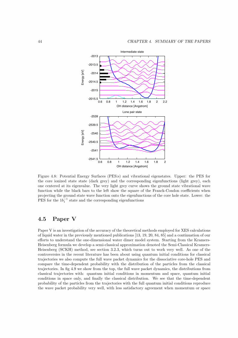


![Simulations and Experiments on the Vibrational Characteristics of …downloads.hindawi.com/journals/sv/2017/2314858.pdf · 2019. 7. 30. · [9] V. F. Zhuravlev, “Theoretical Foundation](https://static.documents.pub/doc/80x56/5fe4282a8c8e9c10e8526da3/simulations-and-experiments-on-the-vibrational-characteristics-of-2019-7-30.jpg)

