Theoretical simulations of environment-sensitive dynamical ...

THESIS FOR THE DEGREE OF LICENTIATE OF ENGINEERING

Theoretical simulations of environment-sensitivedynamical systems for advanced reservoir

computing applications

VASILEIOS ATHANASIOU

Department of Microtechnology and Nanoscience - MC2Chalmers University of Technology

Gothenburg, Sweden, 2018

ii

Theoretical simulations of environment-sensitive dynamical systems for advancedreservoir computing applicationsVASILEIOS ATHANASIOU

c© VASILEIOS ATHANASIOU, 2018. Chalmers University of Technology

Department of Microtechnology and Nanoscience – MC2EMSL LaboratorySE-412 96 Gothenburg, SwedenTelephone + 46 (0)31-772 1000

ISSN 1652-0769Technical Report MC2 - 395

Printed in Gothenburg, Sweden 2018

iii

Theoretical simulations of environment-sensitivedynamical systems for advanced reservoir

computing applications

Vasileios Athanasiou

Department of Microtechnology and Nanoscience - MC2

Chalmers University of Technology

Abstract

The possibility of building intelligent sensing substrates that both collect informa-tion about an environment and analyze it in real-time has been investigated theoret-ically. In a typical setup, a dynamical system is assumed to interact with the environ-ment over time. The system operates as a reservoir computer acting as a reservoirof states. Due to the reservoir-environment interaction, the information about theenvironment is encoded in the state of the reservoir. The information stored in thesystem can be inferred (decoded) by analyzing the reservoir state, which is done byobserving how a system responds to an external stimulus being an external drive sig-nal. This signal is optimized to ensure that under different environmental conditionsthe reservoir visits distinct regions of the configuration space. If such a behavior ispossible, then a relatively simple readout layer can be used to achieve efficient sens-ing. These ideas have been examined theoretically by simulating various networksof environment-sensitive elements: the memristor, the capacitor, the constant phaseelement, and the organic field effect transistor element. It was found that hetero-geneity of the network is important for sensing. The simulations were done in thecontext of ion sensing, which is an extremely complex, many-body, and multi-scalemodeling problem. A generic electrical circuit simulator has been developed with afocus on understanding transient dynamics. The constant phase element has beenidentified as an important primitive that is essential for modeling the experimentaldata. A new algorithm has been develop to model its transient behavior. Likewise,the same was done for the organic electrochemical transistor. To quantify the sens-ing capacity of an environment sensitive network a precise mathematical measurehas been introduced, the state separability index, and evaluated in numerical exper-iments. The theoretical work has been supported by the related set of experiments.

v

“When you sail for Ithaca, wish for the journey to be long, full of adventures, full ofknowledge. ”

Constantinos P. Cavafis

vii

AcknowledgementsFirstly, I would like to express my sincere gratitude to my supervisor Zoran Konkolifor the continuous support of my doctoral studies and related research, for listeningto me and spending time for discussions, for his patience, motivation, and immenseknowledge. His guidance helped me in all the time of research and writing of thisthesis. I could not have imagined having a better supervisor for my doctoral studies.I thank my co-supervisors Aldo Jesorka and Dag Winkler for their useful comments.I thank the collaborators of the RECORD-IT project for the stimulating scientific dis-cussions and for supplying me with useful experimental data.Last but not the least, I would like to thank my family: my wife Christina for spend-ing her life with me and supporting me, my son Alexandros who was born almostin the beginning of my doctoral studies and gave me the power to do research for abetter future of the humanity, to my parents and my brother’s family for supportingme spiritually throughout writing this thesis and my life in general.

ix

Contents

Abstract iii

Acknowledgements vii

List of publications xii

1 Introduction 11.1 Background . . . . . . . . . . . . . . . . . . . . . . . . . . . . . . . . . . 11.2 The relation to the RECORD-IT research project . . . . . . . . . . . . . 21.3 Aim and Scope . . . . . . . . . . . . . . . . . . . . . . . . . . . . . . . . 21.4 Content of the Thesis . . . . . . . . . . . . . . . . . . . . . . . . . . . . . 3

2 Mathematical Primitives 5

3 Part A - Memristor networks as intelligent sensing substrates 93.1 The sensing reservoir model . . . . . . . . . . . . . . . . . . . . . . . . . 9

3.1.1 Sensing with one-memristor network . . . . . . . . . . . . . . . 123.1.2 Towards collaborative sensing . . . . . . . . . . . . . . . . . . . 14

3.2 Results . . . . . . . . . . . . . . . . . . . . . . . . . . . . . . . . . . . . . 173.2.1 A simple classification problem with a one-memristor network 173.2.2 Network structures for environment classification . . . . . . . . 18

3.3 Discussions . . . . . . . . . . . . . . . . . . . . . . . . . . . . . . . . . . 20

4 Part B - Exploiting algorithms for efficient transient simulations 234.1 Transient simulation of electronic circuits with Constant Phase elements 23

4.1.1 Updating the convolution integral . . . . . . . . . . . . . . . . . 244.1.2 Results . . . . . . . . . . . . . . . . . . . . . . . . . . . . . . . . . 264.1.3 Discussions . . . . . . . . . . . . . . . . . . . . . . . . . . . . . . 27

4.2 Transient simulation of electronic circuits with Organic Electrochemi-cal Transistors . . . . . . . . . . . . . . . . . . . . . . . . . . . . . . . . . 294.2.1 Equations of motion . . . . . . . . . . . . . . . . . . . . . . . . . 294.2.2 Fitting the model to data . . . . . . . . . . . . . . . . . . . . . . . 334.2.3 Discussions . . . . . . . . . . . . . . . . . . . . . . . . . . . . . . 33

Bibliography 35

xi

List of Abbreviations

MFB memristor element connected with a delay feedback mechanismNOMFET nanoparticle organic memory field-effect transistorOECT organic electrochemical transistorSWEET state weaving environment echo trackerCPE constant phase elementMNA modified nodal analysisSC sensing capacityODE ordinary differential equationRLC resistor-inductor-capacitorRC resistor-capacitorDC direct currentAC alternating current

xii

List of publications

I. Vasileios Athanasiou & Zoran Konkoli (2017) On using reservoir computingfor sensing applications: exploring environment-sensitive memristor networks,International Journal of Parallel, Emergent and Distributed Systems,DOI: 10.1080/17445760.2017.1287264

II. V. Athanasiou, Z. Konkoli, On the use of collaborative interactions for em-bedded sensing applications: Memristor networks as intelligent sensing sub-strates, Submitted, Under review

III. Athanasiou V, Konkoli Z. On the efficient simulation of electrical circuits withconstant phase elements: The warburg element as a test case. Int J Circ TheorAppl. 2018;46:1072–1090. https://doi.org/10.1002/cta.2474

IV. V. Athanasiou, S. Pecqeuer, D. Vuillaume, Z. Konkoli, On a generic theory ofthe Organic Electrochemical Transistor dynamics, manuscript under prepara-tion

1

Chapter 1

Introduction

1.1 Background

Moore’s law predicts that the number of transistors at the chip doubles roughly ev-ery second year. [21] However, it is likely that this trend will slow down, owing topractical engineering limitations or specific physical effects pertinent to small scales,such as wiring problems or electron tunneling. There are problems that are sim-ply too complex and that cannot be handled by the traditional CMOS technology.In somewhat technical terms, one says that there are information processing ap-plications that do not scale according to the Moore law. Typical examples includeproblems in distributed, real-time, or embedded information processing applica-tions. Accordingly, there is a need to develop alternative information processingsolutions by using non-CMOS based technologies. In the information processingindustry, and especially semiconductor industry, one talks about functional diversifi-cation. The field of unconventional computation has emerged as a response to thisfunctional diversification challenge. Up to date unconventional computation en-compasses a plethora of computing frameworks, such as neuromorphic computing,molecular computing, reaction-diffusion computing, or quantum computing, and isever increasing in its scope. [28, 9, 10, 1, 2, 17]

In particular, reservoir computing has gained a considerable interest among theunconventional computation community in the recent decade, both as a model ofcomputation and as a remarkably practical approach for realizing neuromorphiccomputation. Historically, the field of reservoir computing started as an insightabout behavior of synaptic weights during the neural network training process. [13,12, 20, 29] During the supervised learning the weights need to be adjusted to achievea desired computation. It has been realized that only a limited set of weights is ad-justed in the network training process. While it is true that a neural network is es-sentially a geometry free object, the weights that change belong mostly to the linksin the network that can be naturally described as an “outer layer”. This led to thefurther insight that instead of neural network one could use an arbitrary dynamicalsystem as the core, and augment it with the outer layer. The dynamical system usedthis way is referred to as a reservoir, and the outer layer is referred to as the readoutlayer. The modern understanding of reservoir computing emphasizes the fact that aTuring universal expressive power can be achieved in the context of time-series dataprocessing, if the reservoir exhibits separation property on the state of inputs. Thisseparation property is rather generic, it is not limiting in the engineering sense, andis often realized by complex systems at the edge of chaos. [19]

Though the foundational ideas behind reservoir computing have been aroundfor quite some time, this is still an aggressively developing field which is gainingin momentum. A reservoir computer is essentially a pattern recognition device. Itconsists of two parts, a dynamical system, referred to as the reservoir, that can be

2 Chapter 1. Introduction

driven by the external signal, and an easily trainable readout layer. The external sig-nal is the input accepted by the system. By assumption, the readout layer is the onlypart of the device that can be optimized. The external signal drives the system to aspecific region of the configuration space, which constitutes the act of computationsince the information stored in the external signal is transformed into the informa-tion stored in the internal state of the reservoir. The term “reservoir” stands for thereservoir of states. The readout layer is only used to assess in which state the reser-voir is. The key claim is that any computation can be realized this way, provided thedynamical system is complex enough. Due to the inherent flexibility and the ease ofuse the reservoir computing approach is being applied frequently in many applica-tions that require neuromorphic computation. The reservoir computer can be usedwith a minimum of preparation as an artificial intelligence unit that process exter-nal information. From the theoretical point of view, the specific feature that makesreservoir computing popular is the ease of training. Likewise, from the engineeringpoint of view, the readout layer can be a relatively simple structure.

The sensing reservoir concept: The work done in this thesis focuses on other,entirely novel aspect of reservoir computing. We investigate whether it is possible touse reservoir computing to build intelligent sensing substrates that can both collectand analyze information at the same time. The key idea is that the environment onewishes to sense interacts with a dynamical system, which we refer to as a sensingreservoir, or a state weaver. The sensing reservoir accumulates, or weaves in, theinformation about the environment into its internal state over time. In such a setupthe flow of information is not linear (from the sensor to the artificial intelligenceunit), but the sensor and the associated information processing intelligence are thesame. More details on these ideas can be found in [16, 18] and in section 3.

1.2 The relation to the RECORD-IT research project

This thesis work has been strongly aligned with the activities in the RECORD-ITresearch project. The aim of the RECORD-IT project is to develop an intelligentbiocompatible device sensitive to the environmental changes in ion concentrations.Thus many of the ideas presented in the thesis have been motivated by a need tounderstand the RECORD-IT experiments. The systems of interest feature elementsthat can be described as wet nanoparticle organic memory field-effect transistors(NOMFETs), coated Si nanowires, self-conjugated polymers, or arrays of photocells.These elements are combined to build powerful sensing devices. A natural theoret-ical paradigm for modelling these structures is a network of environment sensitiveelectrical components. This defines the context in which this thesis work has beendone.

1.3 Aim and Scope

The overarching aim has been to exploit theoretically the possibility of using en-vironment sensitive electrical circuit networks as intelligent sensing substrates. Akey feature that is investigated is how the coupling between the elements affectsthe sensing capacity of the device. The hypothesis is that the existing interactionsbetween the network elements should increase the sensing capacity of the network.The key idea is that the spatial-temporal information about the environment can beaccumulated in the state of the reservoir if the system is arranged properly. [18, 16]This could happen if small pieces of information that are scattered over time, and

1.4. Content of the Thesis 3

that might be ignored in the standard sensing setup, can be accumulated, ampli-fied, and ultimately stored in the state of the network. When should one use sucha device? The use of such devices would be advantageous in situations where em-bedded information processing is necessary, e.g. in the case of distributed sensingnetworks. If the information collected by sensors can be pre-processed in situ, thiswould reduce the necessary communication bandwidth, provide real-time analysisoptions, and accordingly make the whole system much more responsive. Moreover,from the engineering point of view, such sensing solutions could be more flexibleand easier to implement, be low-power, or be bio-compatible.

1.4 Content of the Thesis

The content of the thesis follows the structure of the papers I - III which have beeneither published or submitted. This is augmented with a highlights from the veryrecent on-going work, a manuscript in preparation, paper IV.

In paper I it is demonstrated theoretically on a very simple classification problemthat a single memristor can be used to classify the environment it is exposed to. Onlytwo environmental conditions have been considered, describing a static and a vary-ing environment. First, a suitable drive signal has been identified based on intuitiveanalysis of the memristor dynamics. Then, a rigorous mathematical optimizationproblem has been set up, and solved using genetic algorithms. Interestingly, theoptimization algorithm produced another drive signal. The two drive signals aredifferent from each other because the intuitive drive was a square-wave while theoptimization algorithm was allowed to search in the space of more complex sinu-soidal drive signals. Under both drives the memristance is driven to two differentregions of the one-dimensional state space (under the influence of the two envi-ronmental conditions). The environment can be easily inferred by monitoring thememristance value, i.e. if it is “high” or “low”. The separation only occurs if there isa synchronization between the drive and the environmental signals. To quantify themagnitude of the separation, a quality of sensing index was introduced: The abilityto sense depends critically on the synchronization between the drive and environ-mental conditions. If this synchronization is not maintained the quality of sensingdeteriorates.

In paper II, the cooperative behavior between memristor components has beenexplored achieving an additional functionality. In particular, we investigated howthe interplay between various network features influences the sensing capacity ofthe device. The features of interest included the number of network elements, theirconnectivity pattern, and the complexity of the individual element. The big ques-tions which have been addressed are as follows:

• Is it possible to quantify in a rigorous mathematical sense the sensing capacityof the device?

• How much information about the environment can be ultimately stored in thestate of the substrate?

• How is the sensing capacity of the device depends on the number of the envi-ronment sensitive elements in the network?

• Which topological features of the network strongly influence the sensing ca-pacity?

4 Chapter 1. Introduction

In paper III, a new method has been introduced for the efficient simulation ofelectronic circuits which contain Constant Phase Elements (CPEs). Finally, this pa-per suggests an algorithm for simulating circuits with CPEs based on the ModifiedNodal Analysis (MNA). The algorithmic complexity of the suggested algorithm islinear with the total time of the transient simulation. This algorithm is comparedto a simple method found in the literature: the consideration of resistance-capacitorcircuits with equivalent impedance to the CPEs. The comparison has been done bothin terms of the accuracy and the algorithmic complexity.

Paper IV is a typical device modelling paper. A simple dynamical model ofthe Organic Electrochemical Transistor (OECT) element has been suggested and im-plemented for simulation purposes. The model has been systematically improvedthrough a series of carefully designed numerical experiments. The key outcome ofthis work is a rigorous simulation algorithm that can be used to predict the responseof the OECT changes in time, depending on the voltages that are applied at its pins.A key challenge that has been addressed was to explain intriguing peaks in the ex-perimental data for the drain current as a function of time.

5

Chapter 2

Mathematical Primitives

In here some key mathematical primitives of the reservoir computing approach forsensing are explained. These mathematical primitives feature frequently in the workand manifest themselves in many different forms.

The filter is a mapping that converts an input series of data q ≡ q(t)t∈I into anoutput time series data x ≡ x(t)t∈I ,

q F−→ x (2.1)

where I denotes the index set. The individual values in the series are indexed by thevariable t, e.g. as q(t) or x(t). In the following the index set will be omitted whenirrelevant for a discussion. The operation of the filter is denoted as

x = F [q] (2.2)

and a specific value indexed by t can be selected as x(t) = F [x](t). Further, theinput and output data types do not need to match at all. For example, a filter F cantake a vectorial data as the input, a series of values (q(t), u(t)t with q, u ∈ R andproduce a single valued series x(t)t with x ∈ R as the output, with R being the setof real numbers. For a given index t one has x(t) = F [q, u](t).

The reservoir is a special type of a filter. It is a generic dynamical system, tobe denoted by R, that responds to a time-dependent external signal q(t) in a waythat the state of the system x at a particular time instance t depends on the way thesystem has been driven in the past. Using the filter notation introduced above, thisbehavior is represented as

x(t) = R[q](t) (2.3)

In this case the index set I is meant to describe the flow of time. Note that theequation does not read x(t) = R(q(t)), which would imply that the state of thesystem is an instantaneous function of the drive.

The reservoir should have another important property: one should be able toquery its state. Further, the apparatus used to query the state should be somethingsimple, with a low degree of computational complexity, and presumably somethingthat is easy to engineer. The readout layer, to be denoted by ψ, analyses the instan-taneous state of the device x and produces the output y

y(t) = ψ(x(t)) (2.4)

Note that the equation does not read y(t) = ψ[x](t) which would imply that ψ rep-resents a filter.

The key claim of reservoir computing: The abstract mathematical formulationsintroduced above formalize the reservoir computing ideas. Clearly, without stating

6 Chapter 2. Mathematical Primitives

what the expressive power of this model of computation is, the mathematical prim-itives are an empty shell without substance. What gives substance to the field is theclaim that if the filterR has some well-defined mathematical properties, notably if itseparates the input, then any computation is possible with one and the same reser-voir R. Thus for every desired pattern recognition task Φ[q](t), it is possible to finda related readout layer ψΦ such that

Φ[q](t) = ψΦ(R[q](t)) (2.5)

This implies that a single dynamical system has, in principle, infinite computingpower, i.e. it can be used to compute anything. At first this might sound as animpossible claim, but in fact this key insight from the liquid state machine modelrests on rigorous mathematical foundations of the Stone Weierstrass Approximationtheorem. [29].

The sensing goal: Every sensing procedure is done with a certain goal in mind.For example, one might be interested in inferring whether a solution containing ionsis static or changes in time. Thus a sensing procedure can be formally described as apattern recognition task, described by the filter φ,

ϕ(t) = Φ[q](t) (2.6)

The filter is constructed so that its output, the variable ϕ(t), convey the patternrecognition information. For example, the filter could be constructed to output ϕ ≈ 0for static ion concentration, or ϕ ≈ 1 for a varying one. It is useful to think of Φ as aninfinitely “intelligent” neural network that can be trained for any pattern recognitiontask.

The sensing reservoir is a special dynamical system that can be driven by anexternal input and interacts with the environment. Thus the state of the system, inthe filter notation, can be written as

x(t) = R[u, q](t) (2.7)

The sensing performed by the reservoir is represented as

y(t) = S [u, q](t) = ψ(x(t)) (2.8)

where y(t) is the variable that conveys the result of the sensing measurement. Thekey idea pursued in this thesis is that all the sensing functionality should be done by thereservoir, and not the readout layer. Thus the readout layer should be something simpleto engineer with a low degree of computational complexity. As an example of areservoir acting as a filter see Fig. 2.1.

Sensor optimization: The goal is to optimize the sensing reservoir so that it mim-ics the behavior of Φ: Formally, one tries to achieve that y(t) ≈ ϕ(t) to the largestextent possible, uniformly over time. This defines a rigorous mathematical opti-mization problem, where the goal is to find the drive such that

u∗ = argminuδ[u, q] (2.9)

where δ[u, q] is a measure of how well the prediction of the sensing reservoir matchesthe desired classification,

δ[u, q] ≡ ||S [u, q](t)−Φ[q](t)||t (2.10)

Chapter 2. Mathematical Primitives 7

(!)

"(!)

#(!)

! = [", #](!)

!

#(!) Stable Varying Stable Varying

y(!)

1

0

FIGURE 2.1: A hand drawn illustration of the sensing reservoir con-cept (a modification of a figure from [16]). The reservoir is denotedby R with the state of the reservoir at time t denoted by x(t). Thisstate depends on the whole history of the drive signal u(t) and theenvironmental condition signal q(t). To optimize the sensor, a drivesignal u(t) has to be found such that the output y(t) is driven to 1 ifthe environmental condition is a varying one, and to 0 if the environ-

mental condition can be characterized as a stable one.

with ||...||t being a measure of the distance between two filters, the one realized bythe reservoirR and the one by Φ. The subscript on the distance symbol indicates thatone should in some sense provide a distance estimate over all times. For example,one could define the distance as

||S [u, q](t)−Φ[q](t)||2t ≡ limT→∞

1T

∫ T

0dt S [u, q](t)−Φ[q](t)2 (2.11)

which is the definition used in the thesis. The distance measure generated this waywill be denoted as δ∗[u, q].

9

Chapter 3

Part A - Memristor networks asintelligent sensing substrates

Part A of this thesis summarizes the work done on memristor networks in papersI and II. We describe how the mathematical primitives from Chapter 2 have beenimplemented in the memristor network context, with the focus on advanced sensingapplication of ionic concentrations. The memristor is one of the simplest electronicelements which behaves as a filter. Further, it is straight forward to couple suchelements into a network. The response of such a network, at a given time instance,resembles the one of a pure resistor network. The filter property, i.e. the memoryof the past, resides in the resistances which change over time. We studied suchnetworks to streamline the theoretical foundations of the reservoir computing forsensing approach, and critically evaluate the workings of the sensing reservoir idea.

3.1 The sensing reservoir model

An implementation of the sensing reservoir idea using a memristor network is shownin Fig. 3.1. The memristor network is used as a dynamical system, the reservoir R.The memristor network naturally implements the filter primitive since the memris-tance changes in time depending on the voltages that are applied at the externalcontacts of the element: R = f (V1, V2), where here and in the following the dot overa symbol defines a time derivative. The law that describes the rate of the memris-tance change is shown in Fig. 3.2. Thus x(t) depends on the whole past of the drivesignal u and environmental condition q, i.e. the time-series of u, q and not their in-stantaneous values. In the case of the memristor network the most natural way torealize the external drive is by applying external voltages.

The memristor model used in this thesis has been suggested in [24]. The mem-ristance R changes in time depending on the applied voltage across the element ∆V,and other device parameters αM, βM, Vthr, Rmin and Rmax,

R(t) = fM[∆V(t), αM, βM, Vthr] θ[RM(t)− RM,min] θ[RM,max − RM(t)] (3.1)

where t denotes time, θ(x) is the step function [θ(x > 0) = 1, θ(x ≤ 0) = 0]. Pa-rameters αM and βM control how fast the memristance changes, Vthr is the thresholdvoltage, Rmin and Rmax denote the minimum and the maximum values of the resis-tance; the resistance of a memristor cannot be lower than Rmin or higher than Rmax.A typical behavior of fM is illustrated in Fig. 3.2.

The environment model: By assumption, the network is affected by the envi-ronmental conditions of the ionic solutions surrounding it. The key challenge is toassume a suitable model for the environment-reservoir interaction. There are nu-merous options, and special care has been given to choosing an appropriate model.

10 Chapter 3. Part A - Memristor networks as intelligent sensing substrates

Input: Environmental condition

Sensor: Reservoir as a Memristor network

Readout

layerClassification: ion-memristor interactions

-

-

-

-

- -

+

+ +

+ +

+

++ +

+

+

+

+

+

-

-

-

-

- -

-

-

-

-

Drive: Voltage source

FIGURE 3.1: The memristor network is driven by a drive signal andis affected by the environmental conditions of ionic solutions. Thereadout layer receives the instantaneous values of the network stateand contributes to the classification of the environmental condition.

In paper I, based on a careful literature study, it has been argued that it is reason-able to assume that the rate of the memristance change should depend on the ion-concentration. Thus, for simulation purposes, it has been assumed that the parame-ter βM is environment sensitive. Assuming that the variations of the environmentalsignal are small, one can use the standard working point model used in electronics:βM = a + bq(t). This behavior is illustrated in Fig. 3.2. The slope of graph changesdepending on the environmental signal.

The state of the whole memristor network x at time t is described as an orderedlist of resistances for each time instance

x(t) ≡ (R1(t), R2(t), · · · , RNR(t)) (3.2)

where NR is the dimensionality of the state and denotes the number of memristorsin a network. The variable x(t) denotes the trajectory in the state space. This isillustrated in Fig. 3.3. Further, the figure illustrates the operation of the readoutlayer. The readout layer is assumed to be able to access the values of the individualresistances, which provides the output of the computation

y(t) = ψ(x1(t), x2(t), · · · , xN(t)) (3.3)

Now the meaning of the equation x(t) = R[u, q](t) should be transparent: thenetwork is driven by external voltages, and resistances change according to the spec-ified law. The state depends on the whole history of the drive u and the environmen-tal condition q. The state can be given as input to a readout layer which infers theenvironmental condition. The simplest form of a readout layer is given, being aweighted linear sum of the network memristances.

Supervised learning and fitness function: How does one optimize the device

3.1. The sensing reservoir model 11

FIGURE 3.2: The rate of memristance change R ≡ dR/dt depicted asa function of the voltage drop across the memristor element ∆V. Thememristance change is depicted for two cases. All parameters are thesame for both cases except for βM being larger for the model plotted

with the solid line than the model plotted with the dashed line.

![", #]($)

%[", #]($)

&'[", #]($)

u(t)

× *!

× *%

× *&'

output:

+ ", # $ = *- . *! ! ", # $ . /. *&' &' ", # $

FIGURE 3.3: The state of the memristor network is a vector of all thememristances included in the network. The network is driven by asignal u. The output y(t) is as a linear combination of the memris-

tance values.


then for a particular pattern recognition task? One of the recurring challenges in thisthesis is to, for a given network, find a drive signal u∗ that maximizes the sensingcapacity SC[u, q]:

u∗ = argmaxuSC[u, q] (3.4)

It is hard to define the sensing capacity rigorously. We posit that the sensing capacityshould be related to the state space separability. In some sense, the sensing capacityshould be a function of the differences δ[u, q]. In machine learning one measures thetotal prediction error,

ε = ∑q

δ[u, q] (3.5)

and a viable definition of the sensing capacity measure would be

SC[u, q] ∼ 1ε

(3.6)

indicating that a small prediction error should be associated with a large fitness.However, we have often used a slightly different estimate

SC[u, q] ∼∑q

1δ[u, q]

(3.7)

Herein, the sensing capacity SC[u, q] has been introduced to be used as a commonmetric in both papers I and II.

Papers I and II critically assess which dynamical features of the memristor net-work could possibly control the sensing capacity. The key insight from these stud-ies is that the trajectory separation in the phase space controls the sensing capacity.Mathematically, this can be formalized as the following requirement. Let q1, q2, · · · , qEdenote the set of distinct environmental conditions we wish to classify. If the drivesignal is found such as the state of the memristor network (or any reservoir or in-terest) occupies different regions Ω1, Ω2, · · · , ΩE, when exposed to the conditionsq1, q2, · · · , qE then a classification is possible. In particular, if the separation of thetrajectories is strong, the classification could be achieved with relatively simple read-out layer, e.g. a linear classifier might be sufficient.

3.1.1 Sensing with one-memristor network

The simplest possible network, a single-memristor network, has been trained to han-dle a classification problem with two environments. Since the emphasis is on testingthe overall workings of the method, a relatively simply classification problem hasbeen chosen. The goal is to distinguish between two different environments, a sta-ble and a varying one. These were represented by a relatively simple signal pairdenoted by q1 and q2 and shown Fig. 3.4. The figure has been taken from paper I.Normally, in the supervised learning approach, a class is represented by a group ofsimilar signals, but we have considered only one signal per class. In such a way it ispossible to have an intuitive understanding how the optimal drive should look like.

As discussed in chapter 2, this classification problem can be represented as anoptimization problem where the goal is to minimize the distances between the clas-sification performed by the system and the desired classification. The goal is to train


FIGURE 3.4: Figure taken from paper I. The environmental condi-tions which are denoted as q1 and q2.

the system, i.e. to find the drive u∗, so that the sensing is done as

S[u∗, q1] ≈ Φ[q1] (3.8)S[u∗, q2] ≈ Φ[q2] (3.9)

where the pattern recognition problem that needs to be learned by the memristor isgiven by Φ[q1](t) = 0 and Φ[q2](t) = 1.

The above optimization problem has been solved using genetic algorithms, wherewe used the following fitness function as the optimization goal:

SC1[u] = ∑q

1δ∗[u, q]

(3.10)

The sum is over environmental conditions. Effectively, the fitness function above,describes the fact that the goal is to find the smallest possible distances for everyenvironmental condition. If both distances are small, SC1 is large.

A drive signal was found firstly by direct intuitive reasoning. The dynamics ofthe memristor element were analyzed and we had a good understanding of howto choose a drive signal to lead the memristance to a specific direction under onespecific environmental conditions. Therefore, for the two environmental conditionswe identified a drive signal for the memristance to occupy two different regionsunder the two environmental conditions respectively. This intuitive solution wasfound to be in a good agreement with the drive obtained by running the geneticalgorithm. The output for those two drive signals and each of the environmentalconditions q1 and q2 is shown in Figs. 3.8 and 3.9. Interestingly, under the optimizeddrive the output is driven faster to the target values Φ[q](t) but there is a largervariance around Φ[q1] and Φ[q2].

The figures illustrate nicely the phase space separability idea. The output hasbeen driven to different regions for the two environmental conditions. However,since the drive signal has been optimized only on two environmental conditions,then, it would be expected that this drive signal cannot be used generally to classifystable and varying environmental signals. This expectation has been confirmed bynumerically experiments.


3.1.2 Towards collaborative sensing

The key result of paper I is that a one-memristor network can be used for classifyingtwo environment time-series q1 and q2. This indicates that a many-memristor net-work, with many different memristors, could be used to separate between differentfeatures of the environmental conditions, and perform a generic classification. Thishas been investigated in paper II where the classification task is the same as in paperI, i.e. the network should distinguish between a varying or a stable environment.However, to test how well the system generalizes, a larger number of environmen-tal conditions is considered. Every environment qi is represented as group of signalsqi ≡ qa

i ; a ∈ Ei where Ei is the index set that describes the environment qi.The simulations were done to investigate a specific idea. One-memristor of the

network could contribute to the separation based on different features between aconstant environment qa

1 and a varying qa2 and another memristor could contribute

on the separation based on other different features between a constant environmentqb

1 and a varying environment qb2. For this to be done, all the memristor elements

ought to be connected so that the separation of different features can be distributedamong the network elements.

Assuming that a collaboration between memristor elements can be exploited asadvocated, how should they be connected into a network for the best possible ef-fect? In paper II, we have attempted to answer this very broad question. We haveinvestigated how the number of network elements, their connectivity pattern andthe complexity of the elements affect the sensing capacity of the network. Thus thebig questions of paper II are as follows:

• How can one quantify the sensing capacity of the device without consideringthe readout layer? An equivalent question is, how much information about theenvironment can be stored in the state of the substrate?

• Is the sensing capacity necessarily favored by an increased number of the envi-ronment sensitive elements or is there an upper bound of the sensing capacitythat cannot not be exceeded?

• Which connectivity pattern are favorable for a larger sensing capacity? In par-ticular, can delay feedback mechanisms be used with an advantage?

The time series of the environmental conditions (the training data) are shownin Fig. 3.5. These conditions will be called the training data since the drive signalhas been optimized for these conditions. The training data are labeled with theircorresponding class and therefore finding the optimum drive signal is a supervisedlearning task. In order to test whether the optimum network can be generally usedfor classifying stable and varying environmental conditions, we created a biggerlabeled dataset, the testing data. The testing data consists of thousand randomlycreated conditions accompanied with the label of their corresponding class.

In paper II, we have not considered a readout layer because we did not want thereadout layer to affect the optimization process, or influence the conclusions. If thesensing capacity of the network is relatively large then a simple readout layer wouldbe sufficient for implementing the classification task. An attempt has been made tofocus exclusively on the sensing capacity of the reservoir per se. There is a dangerthat the readout layer actively participates in sensing, and it is hard to control itscomputational complexity. In papers I and II, the sensing capacity of the networkwas based on measuring the interclass separability, i.e. when the network is driven


Class 0: Stable environmental conditions

(10 randomly generated conditions)

Class 1: Varying environmental conditions

(10 randomly generated conditions)

Training data

a b

FIGURE 3.5: Figure taken from paper II. The training data for the twodifferent classes. a) The training data for Class 0 b) The training data

for class 1.

!"#($)

!"%($)

t

&'(*)

!"#($)

!"%($)

+,-

t

&'(*)

Low separability index . Large separability index .a) b)

FIGURE 3.6: a) An example of low separability index ν. When thememristance R0 is driven on average to similar regions under bothenvironmental conditions q1 and q2, then this contributes to decreas-ing the separability index ν. b)When the memristance R0 is driven on

average to different regions then this contributes to increasing ν.

by different environmental conditions, then the state should be driven to differentregions. In paper I, due to the fact that the state is one-dimensional, the intraclassseparability is a consequence of interclass separability.

In paper II we developed a measure which is indicative of the state separation,the separability index ν. The concept behind the definition of the index ν is illus-trated in Fig. 3.6. In Fig. 3.6a, the memristance R0 is driven on average to similarregions under different environmental conditions and that would make the sepa-rability index lower. In Fig. 3.6b, the memristance R0 is driven on average to twodifferent regions under two different environmental conditions, leading to a largerseparability index.

Mathematically, the ideas discussed above were implemented as follows. Themean value of the mth memristance of a network under the environmental conditionqa

i is given as:

Rm[u, qai ] =

1T

∫ T

0dtRm[u, qi

j](t) (3.11)

For a given network with NR memristors and under a drive signal u, the distancebetween two environmental conditions belonging to classes i and j, qa

i and qbj , is


NFB1

MFB unit

NFB2

FIGURE 3.7: Figure taken from paper II. In network NFB1, the de-layed signal is added to the provided drive. In the network NFB2an MFB unit is added. The memristance signal R1 is converted to

voltage and is used to drive the added MFB unit.

given as:

di,aj,b =

√√√√ 1NR

NR

∑m=1

(Rm[u, qa

i ]− Rm[u, qbj ])2

(3.12)

Totally, for a given network, a drive signal u and a set of training data with classesc1, c2, · · · , ck, the index ν is calculated as the geometric mean of all the possible ND

distances di,aj,b

The structures of the memristor networks were investigated in two ways. Firstly,the complexity of the network topology was increased by adding memristors in par-allel and in series. Six networks were considered: N1, N2, · · · , N6 with the numberof memristors given by NR = 1, NR = 2, · · · , NR = 6 respectively. Secondly, thecomplexity of the elements was increased by introducing the MFB element: a mem-ristor with a time-delay feedback loops. We used time-delay feedback loops becausethe system is expected to gain additional memory properties. The MFB unit at thetime t keeps track of the memristance of a previous time with a delay τ, R(t− τ), andconverts it to a voltage signal with a linear mapping. The converted voltage is addedto the voltage signal across another memristor element. An example is given in Fig.3.7 which shows two networks the NFB1 and the NFB2 with 1 and 2 MFB unitsrespectively. In the network NFB2 an MFB unit is added to the network NFB1: Thememristance signal of NFB1 is converted to voltage and is used to drive the addedMFB unit. Similarly, the network NFB3 was considered by adding an MFB unitto NFB2, the network NFB4 by adding an MFB unit to NFB3. In a similar way,NFB5 and NFB6 networks were considered. For the networks NFB2, NFB3, · · · ,NFB6, the time delays of the MFB units were also considered as free parameters tobe optimized.

3.2. Results 17

q=q1

q=q2

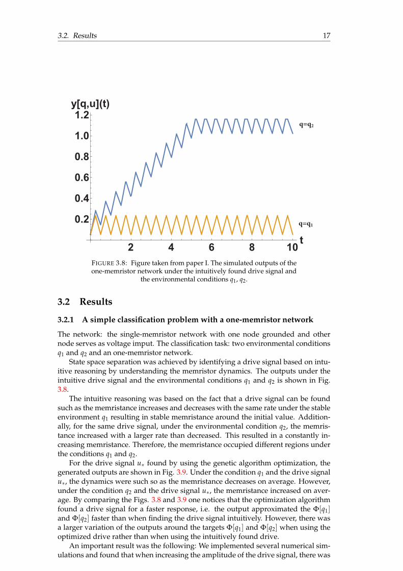
FIGURE 3.8: Figure taken from paper I. The simulated outputs of theone-memristor network under the intuitively found drive signal and

the environmental conditions q1, q2.

3.2 Results

3.2.1 A simple classification problem with a one-memristor network

The network: the single-memristor network with one node grounded and othernode serves as voltage imput. The classification task: two environmental conditionsq1 and q2 and an one-memristor network.

State space separation was achieved by identifying a drive signal based on intu-itive reasoning by understanding the memristor dynamics. The outputs under theintuitive drive signal and the environmental conditions q1 and q2 is shown in Fig.3.8.

The intuitive reasoning was based on the fact that a drive signal can be foundsuch as the memristance increases and decreases with the same rate under the stableenvironment q1 resulting in stable memristance around the initial value. Addition-ally, for the same drive signal, under the environmental condition q2, the memris-tance increased with a larger rate than decreased. This resulted in a constantly in-creasing memristance. Therefore, the memristance occupied different regions underthe conditions q1 and q2.

For the drive signal u∗ found by using the genetic algorithm optimization, thegenerated outputs are shown in Fig. 3.9. Under the condition q1 and the drive signalu∗, the dynamics were such so as the memristance decreases on average. However,under the condition q2 and the drive signal u∗, the memristance increased on aver-age. By comparing the Figs. 3.8 and 3.9 one notices that the optimization algorithmfound a drive signal for a faster response, i.e. the output approximated the Φ[q1]and Φ[q2] faster than when finding the drive signal intuitively. However, there wasa larger variation of the outputs around the targets Φ[q1] and Φ[q2] when using theoptimized drive rather than when using the intuitively found drive.

An important result was the following: We implemented several numerical sim-ulations and found that when increasing the amplitude of the drive signal, there was


q=q1

q=q2

FIGURE 3.9: Figure taken from paper I. The simulated outputs of theone-memristor network under the optimum drive signal (from the

genetic algorithm) and the environmental conditions q1 and q2.

a faster response and a larger variation around the target Φ[q]. This indicates thatthere is a trade-off between time response and variation around the target Φ[q].

3.2.2 Network structures for environment classification

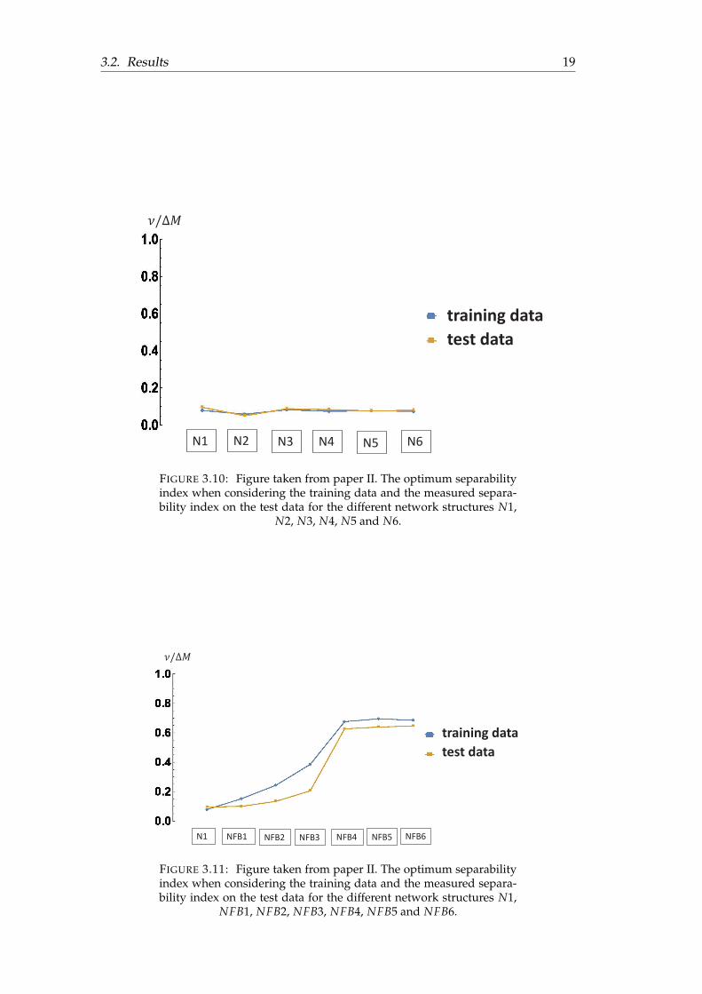
In this section, the optimum separability index ν is shown for the different memristornetworks studied. The index ν was maximized by training the memristor networkswith the training data. Additionally, to evaluate the performance of the optimizednetworks, we measured the separability index on the test data. The index ν forboth cases is shown in Fig. 3.10, when the networks were constructed by adding inparallel and in series memristors, and in Fig. 3.11, when the MFB units were used.

In Fig. 3.10 it is shown that the separability index did not increase when addingmemristor elements in parallel and in series. With such network structures there isno adequate collaboration between the memristor elements.

In Fig. 3.11 it was shown that the increase of the elements complexity favoreda larger separability index. More specifically, in this figure, as the dimension of thestate increases from (NR = 1 for N1) towards (NR = 4 for NFB4), then, the separabil-ity index on both training and test increased. This means that elements collaboratewhen added into the network. Additionally, the index ν did not improve consid-erably for both the training and the test data when adding MFB units to NFB4.Therefore, NFB4 can be considered as the network with the minimum amount ofresources for achieving the largest index ν. One can also notice in Fig. 3.11 that theindex ν on the testing data is favored by an increased number of MFB units. Espe-cially, the distance between the index ν on training and testing data tends to be verysmall when considering the network NFB6. This happens because when the dimen-sionality of the state increases, then, there are more chances for the state to occupydifferent regions for different environmental conditions.

3.2. Results 19

N1 N2 N3 N4 N5 N6

/!"

training data

test data

FIGURE 3.10: Figure taken from paper II. The optimum separabilityindex when considering the training data and the measured separa-bility index on the test data for the different network structures N1,

N2, N3, N4, N5 and N6.

N1 NFB1 NFB2 NFB3 NFB4 NFB5 NFB6

/!"

training data

test data

FIGURE 3.11: Figure taken from paper II. The optimum separabilityindex when considering the training data and the measured separa-bility index on the test data for the different network structures N1,

NFB1, NFB2, NFB3, NFB4, NFB5 and NFB6.


3.3 Discussions

In this part of the thesis, the possibility of using networks of environment sensitiveelements for advanced sensing applications has been investigated theoretically, inthe context of the SWEET sensing setup. Memristors were considered as an exampleof environment sensitive elements where a relatively simple model of the interactionbetween the environment and the memristor has been assumed.

There are important lessons to be learned from the numerical work carried outin paper I. These can be used to speculate on the behavior of larger networks withlarger training datasets. The synchronization between the drive signal and the environ-mental conditions is important. A natural question that naturally suggests itself is: Isit still possible to identify a distinct drive signal which synchronizes with a largerdataset of training data? Additionally, the strength of the drive signal was foundto regulate the trade-off between the response time and the error. Here it would bevery interesting to check whether this finding is true for the larger and more com-plex networks considered in paper II. If this is not true, then, it might be that thisfinding is valid only for simple networks of memristors (i.e. connections in paralleland series).

The main question addressed in paper II was: How to design a network toachieve a collaboration between environment sensitive elements? The sensing ca-pacity of the device was found to increase if heterogeneous time delay feedbackmechanisms were used (with different time delays). This is an important finding.It shows that heterogeneity is significant for the performance of the device. However, wefound that after the usage of a specific number of memristors with time delay feed-back mechanisms connected to the network, there was no further increase in thesensing capacity, the sensing capacity reached a plateau.

It is also interesting to notice that the memristor networks in paper II constitutean implementation of an artificial neural network primitive: an important part of theintegrate and fire concept, a highly non-linear function that takes the weighted sumof the inputs to a neuron and produces an output in a given range. By using delayfeedbacks, the memristor elements achieve a similar behavior as neurons: except foradding non-linearity to the network, their memristance can be driven in relativelyshort times to two states of operation, either their maximum (firing state) or mini-mum value (non-firing state). However, in contrary to artificial neural networks, wenoticed that by adding more and more complex elements to the network, the sep-arability index on the test data did not worsen, i.e. overfitting was not a problem.We argue that this happened because the dimensionality of the state space increasedand there were few chances for the state to occupy similar regions of the state underdifferent environmental conditions.

Possibly, if we implemented numerical experiments with larger networks, then,we could see effects of overfitting. This poses a question: for a given classificationtask, who performs better, the neural network or a memristor network? For choos-ing whether to use complex memristor networks (with delay feedback units) as sug-gested in paper II, or software based solution (e.g. artificial neural networks), deci-sive factors would be the cost (in energy or hardware) to use delay feedback mech-anisms. Additionally, memristor networks and artificial neural networks could beused together in hybrid solutions, where the output of memristor networks, whichperform hardware computations, could be used as input in software based artificialneural networks.

In this thesis, we constructed a simple way to measure the state separation with asimple number and introduced the separability index ν. Clearly, there could be other

3.3. Discussions 21

ways for estimating the sensing capacity by accounting the temporal behavior of thesignals representing the state. For example, a way would be to use a generic mea-sure of the mutual information concept to quantify how much information aboutthe environment is stored in the state of the system. Another would be sensing byidentifying specific patterns at the state of the network.

The concepts developed in this part are intended to be used in the RECORD-ITproject. Already, an experimentalist group involved in the RECORD-IT project haveimplemented the ideas of heterogeneity in time delay feedbacks. They have used intheir system two different time delay feedbacks and they have noticed sensitivity ofthe state to the chemical concentrations around their network of sensors.

23

Chapter 4

Part B - Exploiting algorithms forefficient transient simulations

Part B of this thesis summarizes the work done in papers III and IV. There has beena need to simulate accurately and efficiently several SWEET device prototypes. Wedeveloped a generic electronic circuit simulator for simulating the transient behav-ior of electronic circuits with environment sensitive elements. The ultimate goal wasto use the simulator as an optimization tool to identify optimal network designs (e.g.the drive signal and the network parameters). The simulator has been implementedas an integral part of an automatic genetic algorithm optimization procedure wheremany network designs are tested at random until the one with a desired function-ality is found. Since such a numerical optimization process involves an extremelylarge number of simulations, then, each simulation should be executed in a relativelyshort time, to make such an optimization approach feasible.

While many electronic component models have been imported to the simulatorfrom the literature, e.g. the widely used models for resistor, memristor, capacitor,inductor, some components were modelled from scratch. In particular, a lot of efforthas been put into developing efficient simulation algorithms for the constant phaseelement (CPE) and the organic electrochemical transistor (OECT). CPEs are modelsof electronic circuits that are used in equivalent electronic circuits of elements whereionic diffusion is involved. The OECTs are special purpose devices used for analyz-ing ionic solutions. There is a genuine lack of accurate and algorithmically efficientmodels for simulating OECT and CPE transient behaviors. Further, for the OECTelement of interest, some models are available, but because of their special-purposenature, they have severe limitations and could not be used directly.

In section 4.1, a new method for simulating the transient response of CPEs isgiven. In section 4.2, a generic theory of OECT transistors is given which can beused to develop a model for simulating the transient response of OECTs.

4.1 Transient simulation of electronic circuits with ConstantPhase elements

The problem regarding the transient simulation of electrical circuits with CPEs isthat a repeated numerical evaluation of a computationally expensive convolutionintegral is needed, shown in Eq. (4.1). This integral relates the instantaneous voltagedrop Vw(t) across the element, with the current that has passed through it Iw(t′) witht′ ≤ t. To avoid this problem, various methods have been suggested in the literature.

The standard method is to approximate the CPE element by an equivalent RLCcircuit. [26, 30, 31, 4] These circuits are easier to simulate. For example, there are

24 Chapter 4. Part B - Exploiting algorithms for efficient transient simulations

commercial packages available that can be used to simulate them efficiently. How-ever, these methods are only accurate in a short range of frequencies due to a finite(often a relatively small) number of resistors, capacitors or inductors. The accuracyin a wide range of frequencies requires the increase in the number of elements, andthis increase implies a larger algorithmic complexity cost. It has been pointed out in[4] that the accurate approximation of RLC circuits in a wide range of frequencies isstill an open problem.

Another set of methods focuses on expanding the convolution kernel as an infi-nite series of special functions. [14, 8] The advantage of these approaches is that ifthe series converges fast then only few terms in the series expansion need to be kept.However, in general it is hard to know how many terms should be kept.

We have developed a novel method for simulating the transient dynamics ofCPEs that is both generic, remarkably efficient, and surprisingly accurate. For sim-plicity reasons this thesis focuses on a specific type of CPE, the Warburg element.The Warburg element is one type of CPE where the applied voltage difference Vw attime instance t, Vw(t), and the current passing through it Iw at time instance t, Iw(t)have a phase difference equal to 45 degrees. The method for simulating transientresponse of the Warburg element can be easily extended to CPEs.

The need for developing the new method emerges from the fact that the calcu-lation of the voltage across the CPE, Vw(t), requires the calculation of the followingconvolution integral [15]:

Vw(t) =Aw(αw)

Γ(αw)

∫ t

0(t− u)αw−1 Iw(u) du, αw ∈ [0, 1) (4.1)

with Γ being the usual Gamma function, e.g. Γ(1/2) =√

π, and Aw(αw) is a devicedependent constant.

Calculating numerically the convolution integral is reasonable for short time in-tervals. However, a repeated numerical evaluation of the convolution integral can bevery expensive for long times. Problems arise regarding the memory usage and thecomputation time because the time instances of the current Iw(t) have to be storedfor a long time interval [0, t]. Additionally, the larger this time interval is, the morecomputationally expensive the calculation of this integral becomes. [15] For exam-ple, assuming a grid of n time points t0 = 0, t1, · · · , tm, · · · , tn, the computationalcost of evaluating the convolution integral scales as

O(n2) ∼n

∑m=0

O(m) (4.2)

where O(m) is the algorithmic cost of evaluating the integral for a fixed time instancetm. Paper III suggests a generic method for decreasing the algorithmic complexityby one order of magnitude.

4.1.1 Updating the convolution integral

For the Warburg element, αw = 1/2 and the voltage is calculated as the followingconvolution (’*’ denotes the convolution operation):

Vw(t) =Aw√

π

1√t∗ Iw[t] =

Aw√π

Φw(t) (4.3)

where Aw ≡ Aw(αw = 1/2).

4.1. Transient simulation of electronic circuits with Constant Phase elements 25

The computational cost of any standard quadrature algorithm for the approxi-mation of the convolution integral Φw(tn) in a discrete grid of n time-points t0, t1,· · · , tm, · · · , tn scales with the size of the time grid n, where t0 = 0 and the distancebetween two successive time-points is given as ∆ti = ti − ti−1:

Φw(tm) ≈m

∑j=0

wmj Iw,j (4.4)

where for further convenience we use the notation: Iw,j = Iw(tj) and, the weight wmj

depends on the time-points of the grid tj and tm.While the computational cost of evaluating Eq. (4.4) at a fixed time instance tm is

O(m), the problem is that a repeated evaluation for many time instances leads to aquadratic cost O(n2), and here we assume that the time grid of the simulation con-sists of n time points. To deal with this problem, in paper III, we have developed amethod to calculate the convolution integral at time tm, Φw(tm), by using the alreadycalculated Φw(tm − dt). To do that, the convolution integral Φw(tm) is split in twoparts:

Φw(tm) = H(tm, tλ) + Ψ0(tm, tλ) (4.5)

where,

H(tm, tλ) =∫ tm

tλ

Iw(u) du√t− u

(4.6)

and,

Ψ0(tm, tλ) =∫ tλ

0

Iw(u) du√t− u

(4.7)

where H(tm, tλ) is calculated with high precision and Ψ0(tm, tλ) is calculated by asimple update of the previously calculated Ψ0(tm−1, tλ−1).

The key idea is shown in Fig. 4.1. The One part, Ψ0(tm, tλ), is used to approx-imate the convolution integral between 0 and tλ and the other part, H(tm, tλ), forthe approximation between tλ and tm. At the next time step tm+1, the convolutionintegral is written again a sum of the two parts:

Φw(tm+1) = H(tm+1, tλ+1) + Ψ0(tm+1, tλ+1) (4.8)

Notice here that the successive distances tm − tλ and tm+1 − tλ+1 are approximatelyequal. Therefore, the calculation of H(tm, tλ) would require similar algorithmic com-plexity to the calculation of H(tm+1, tλ+1). However, the calculation of Ψ0(tm+1, tλ+1)requires larger algorithmic complexity than the calculation of Ψ0(tm, tλ) becausetλ+1 > tλ.

Since the algorithmic complexity of calculating H(tm, tλ) is similar at every timepoint tm, we calculate this part with high precision. However, the algorithmic com-plexity of calculating Ψ0(tm, tλ) increases as tm increases.

In paper III, we developed a method where Ψ0 at the next time point, Ψ0(tm+1, tλ+1),can be approximated by a simple update of Ψ0 at the previous time point, Ψ0(tm, tλ).For this purpose, we suggested a dynamical system with N + 1 equations and a clo-sure function. This dynamical system is shown in Eqs. (50) and (51) in paper III. Thedefinition of the closure function is given in Eq. (49) in paper III:

r(tm+1, tλ) =

∫ tλ

0Iw(u) du

(tm+1−u)2·N+3

2∫ tλ

0Iw(u) du

(tm+1−u)2·N+1

2

(4.9)


! ! + " !#$ % % + " %#$

&( %, ')*-( %, ')

&( %#$, '#$)*-( %#$, '#$)

1

% .

12

3

FIGURE 4.1: Figure taken from paper III. The concept of calculatingthe convolution integral at the time-point tm + ∆tm+1 by using theprevious convolution integral at the time-point tm. The integral Φ(tm)( Φ(tm + ∆tm+1)) is calculated by convolution between the currentand the curve reaching the time-point tm (tm + ∆tm+1). The integralΦ(tm + ∆tm+1) is approximated by three different calculations. Re-gion 1 refers to the tail window calculation by using information fromthe previous convolution integral. Regions 2 and 3 refer to analyticalcalculation of the convolution integral by linear interpolating the cur-

rent Iw(t).

One of the questions of this paper is how to calculate the closure function above. Tocalculate it analytically, it has been chosen that the current is constant Iw(u) = Io.

Finally, an algorithm is suggested for performing transient simulations of elec-tronic circuits with Warburg elements by using the Modified Nodal Analysis (MNA).The Warburg element is suggested to be used similarly to a Voltage source objectwith the MNA. The MNA is widely used in electronic circuit simulators for transientsimulations and therefore the integration of the developed method with electroniccircuit simulators is amenable.

4.1.2 Results

In paper III the designed algorithm was tested on a simple circuit driven a voltagesource. Different numerical simulations were performed for two different cases ofthe voltage source signal: DC and AC signals of different frequencies. The size ofthe dynamical system was set for all the simulations as N = 1.

By performing those numerical simulations, we investigated the effect of the dis-tance tm − tλ on the algorithmic complexity and the error. We found that there isa trade-off between the error and the algorithmic complexity. By choosing the dis-tance tm− tλ one can regulate this trade-off. By increasing the distance tm− tλ, then,the error decreases at the cost of a larger execution time of the algorithm.

By comparing our method with a simple RC (resistor-capacitor) circuit, we foundthat the execution time of our method is similar to a Three-RC circuit (with three ca-pacitors and three resistors). This finding is interesting because one would expect amuch larger execution time with our method since our method is heavily dependenton the approximation of H(tm, tλ) being computed with high precision. However,the execution time with RC methods is relatively large due to the larger number of

4.1. Transient simulation of electronic circuits with Constant Phase elements 27

**

*

--

-

>>

>

<<

<

k = 100 k = 200 k=500method

0.5

1.0

1.5

2.0error(%)

* f0

- 103×f0

> 106×f0

< 109×f0

FIGURE 4.2: Figure taken from paper III. The error(%) when the cir-cuit was simulated with an AC voltage source as a sinus signal withamplitude 0.001V and four different cases: with period 1/ f0 = 0.628s,1/(103 f0), 1/(106 f0) and 1/(109 f0) respectively. The time-step dtwas such that 100 time-points were sampled per sinus cycle. The cir-cuit was simulated for five cases: k = 30, k = 100, k = 200, k = 500and k = ∞. The parameter k denotes the number of time-pointswhich have been used to calculate H(tm, tλ) with high precision. Theerror is calculated as the absolute difference between the ideal casek = ∞ and the every other case k = 30, 100, 200, 500 divided by themaximum value of the simulation for k = ∞. In the time domain, theerror is oscillating from 0 to a maximum value. The maximum error isdepicted on the vertical axes. The error(%) when k = 30 is not shownin this figure for resolution reasons. This error was found as 2.54%,

4.17%, 4.69% and 4.71% at the four frequencies respectively.

nodes in the equivalent circuits (6 nodes were used with the Three-RC circuit and 3nodes with our method).

A key result is that our method is stable at a large range of frequencies (1Hz−1GHz) as it is shown in Fig. 4.2. This is a great advantage of our method: The RLCcircuits have equivalent impedance to constant phase elements in a small range offrequencies while our method is stable in very large range of frequencies. If wewanted to use the "Three-RC circuit" method for achieving a low error in a largerrange of frequencies, then, we should design an RC circuit with more componentsand voltage nodes and the algorithmic complexity would be heavily increased.

4.1.3 Discussions

In paper III, a new method has been designed and tested for performing transientsimulations of electrical circuits that contain CPEs. In particular, the problem is thatthe numerical evaluation of the convolution integral describing the response of theWarburg element is computationally very expensive. By default, the convolutionintegral has an algorithmic complexity O(n2) for a grid with n time-points. We iden-tified a way to reduce the algorithmic complexity by one order of magnitude.

One important finding was that the trade-off between error and execution timecan be regulated by the distance tm − tλ. It would be interesting to investigate infuture how the choice of the total number of equations in the dynamical systemaffects this trade-off. This presents an intriguing algorithmic challenge for future work:


We performed some numerical simulations with N > 1 and the error was increasedinstead of our expectations for a decreased error. Therefore, the question is how is itpossible to increase the number of dynamical equations and decrease the error. Sucha finding would be of great significance since a better trade-off between error andexecution time could be found.

Additionally, regarding the analytical calculation of the closure function, onecould argue that it is not reasonable to consider a constant current. A constant cur-rent passing through a CPE means that it will charge (or discharge) for the wholetime of the simulation which is a rare case in experiments. In the simulations un-der both AC and DC voltage source signal, the current was not stable. Therefore, thequestion is if one could use another way to calculate analytically the closure functionand achieve less error. A possibility is to switch between different update schemes asthe simulation progresses.

Finally, the developed methods in paper III can be used to integrate a CPE objectin a simulator operating with Modified Nodal Analysis in a large range of frequen-cies. This has not been achieved before. For example by using RLC methods, e.g.as the one suggested in [26], one should consider a quite large RLC circuit to op-erate with equivalent impedance to CPEs in the range of frequencies 1Hz− 1GHz.However, the simulation of quite large circuits requires quite large execution times.

4.2. Transient simulation of electronic circuits with Organic ElectrochemicalTransistors

29

4.2 Transient simulation of electronic circuits with OrganicElectrochemical Transistors

Transient simulations of electrical circuits with OECTs can be a useful tool for de-signing efficient environment sensitive networks for biosensors applications. Suchsimulations can provide mechanistic understanding of the underlying physical con-cepts. They can be used to infer circuit parameters by fitting simulations to experi-mental data, etc.

In the literature, there have been successful theoretical models which unravel theunderlying principles of OECTs. [3, 25, 7, 5] However, there are limitations regardingthe usage of these models for building simulator primitive that are easily integratedin the electric circuit simulators, e.g. such as SPICE.

For example, Faria et al. [5] have proposed a model for the drain current tran-sient response. Their model is useful for predicting the transient drain current in arange of time when the gate voltage input is known in the whole range before thestart of the simulation. However, when connecting OECTs in a network then thegate voltage cannot be known in the whole range. As an example, the gate volt-age driving one OECT might be dependent on the chemical concentrations aroundother OECTs, and therefore this gate voltage cannot be known before the simulation.Sideris et al [27] have also suggested a method for simulating the OECT transient.Their method is based on polynomial approximations of the drain current.

In paper IV, we have proposed a theoretical setup for describing the OECT tran-sient response when exposed to arbitrary voltage signals at the electrodes. Our ap-proach is more generic than the one by Sideris et al, since it is based on a genuinedynamic ODE paradigm, and allows for more flexible numerical integration tech-niques.

4.2.1 Equations of motion

In our approach, we generalize the equations of motion previously developed byBernards and Malliaras [3], and obtain a system of partial differential equations thatdescribe how ionic degrees of freedom are coupled with the electrical degrees offreedom in the material.

The geometry of both the device and the electrolyte are given in Fig. 4.3. The de-vice is a semiconducting substrate with dimensions L, w, y and is covered by ionicsolution above. The device volume is divided in vertical slices with infinitesimalvolumes, as shown in Fig. 4.3a. Every infinitesimal volume is described by usingthe equivalent circuit model, as shown in Fig. 4.3b. The gate voltage Vg(t) is appliedon the top of the electrolyte. The voltage on the boundary between the semiconduc-tor and the electrolyte at the position x and time t is denoted as Vch(x, t). V(x, t)denotes the voltage inside the electrolyte. This simple model features a resistance Recoupled in series to a capacitor Cd. The resistance describes the flow of ions throughthe slice of the electrolyte above the semiconductor (Fig. 4.3c).

After passing the electrolyte, the ions enter into the semiconductor material. Ithas been argued that a good model that describes this process is a volume capaci-tance. The capacitance of the piece of material with volume v = ywdx is given byCd = cdv where cd is the volume capacitance of the device material (Fig. 4.3d).

In every small volume of the device there is an accumulated charge densityQ(x, t). In the equivalent circuit, this charge density is the charge of the capacitorCd. By solving Kirchhoff laws in the equivalent circuits, the following dynamical


w

y

dx

Device

Electrolyte

z

a) dxb)

!

"#

$%(&)

!

"#

$%(&)

$'*(+, &)

V(+, &)

$'*(+ - .+, &)

V(+ - .+, &)

!

"#

$%(&)

$'*(+ / .+, &)

V(+ / .+, &)

0 0z

y

L

"#

w

z

dx

1 !1

w

dx

y

c) d)

FIGURE 4.3: a) The geometry of the electrolyte and the device is di-vided in infinitesimal slices with length dx. Each slice contains twoparts. The volume dx w y occupies the region in the OECT material.Above this volume, there is a volume of electrolyte dx w z. b) Theequivalent circuits of the device and the electrolyte. The material actsas a volume capacitance where Cd is the capacitance of the devicesub-volume. The electrolyte sub-volume has a resistance Re. Appliedvoltages are: the gate voltage Vg, Vch(x, t) is the time-dependent volt-age at the boundary between electrolyte and device at the positionx, and V(x, t) is the local voltage in the device sub-volume. c) Theelectrolyte is modeled by an equivalent resistance Re. d) The device

is modeled by an equivalent capacitor Cd.


31

equation is derived:

∂Q(x, t)∂t

= −Q(x, t)τ

+1τ

cd y w [Vg(t)−V(x, t)] (4.10)

with the time constant of the equivalent circuit given by τ = recdzy.Across the semiconductor material, the Ohm’s law relates the current density

J(x, t) flowing through the semiconductor device and the voltage V(x, t).

J(x, t) = eµρ(x, t)∂V(x, t)

∂x(4.11)

where ρ(x, t) is the local density of charge carriers, e is the charge of the carrier,and µ is their mobility. The free charge carrier density ρ(x, t) is regulated by theconcentration of ions Q(x, t) that are absorbed in the material: an increase in Q(x, t)leads to a decrease in ρ(x, t). An approximate relationship between ρ and Q has beensuggested in [3]:

ρ(x, t) = ρ0

(1− Q(x, t)

Qmax

)(4.12)

where ρ0 and Qmax are device parameters.Equations (4.11) and (4.10) have been solved and analyzed by making the as-

sumption that the transient charge in the device Q(x, t) can be approximated by thecharge density at the steady state condition Qst(x, t) times a variable T:

Q(x, t) ≈ T(t)Qst[x, ξ(t)] (4.13)

The variable T denotes how far the system is from the steady state condition. IfT = 1, then the system is at the steady state. Otherwise, the system has less charge(T < 1) or more charge (T > 1) than in the steady state condition. The externallycontrolled electrode voltages: gate Voltage Vg(t), drain voltage Vd and source Volt-age Vs are collectively denoted as ξ(t). These voltages determine the stationary statecharge density profile. If ξ is altered, the charge density profile Qst(x) changes too,and to emphasize this we use Qst(x, ξ)

After the straight forward but somewhat tedious algebra, which will not be re-produced here, the solution of the Eq. (4.11) by using the above assumption resultsin an analytical equation for the drain current ID:

ID(t) = fO[T(t), ξ(t)] =

= G

(1−

Vg − Vd2

Vp

)(Vd T)2

T Vd −[Vp (1− T)

]Log

(1 + T Vg

Vp−T Vg

) (4.14)

where G is the conductance of the semiconductor given as G = eµρoW YL and Vp is

the pinch-off voltage of the semiconductor.The analysis of the Eq. (4.10) with the above assumption considering a discrete

time grid with time step ∆t results in the following update rule for the parameter T:

T(t) =τ

τ + ∆tΛ(t, ∆t) T(t− ∆t) +

∆t∆t + τ

Ξ(t) (4.15)


where

Λ(t, ∆t) ≡ 〈Λ(x, t, ∆t)〉x (4.16)Ξ(t) ≡ 〈Ξ(x, t)〉x (4.17)

with

Λ(x, t, ∆t) =Qst[x, ξ(t− ∆t)]

Qst[x, ξ(t)]=

Vg(t− ∆t)−Vst[x, ξ(t− ∆t)]Vg(t)−Vst[x, ξ(t)]

(4.18)

and

Ξ(x, t) =Vg(t)−V[x, T(t), ξ(t)]

Vg(t)−Vst[x, ξ(t)](4.19)

Herein, due to the fact that it is computationally expensive to calculate the integralsin Eqs. (4.16) and (4.17), Λ(t, ∆t) and Ξ(t) are calculated by setting x = L

2 in Eqs.(4.18) and (4.19). It is not set x = 0 or x = L because there are not transient dynamicsat the bounds.

The parameter Ξ(t) indicates how far the transient dynamics is from the steadystate conditions. If V[x, T(t), ξ(t)] = Vst[x, ξ(t)], then, T = 1 and Ξ(t) = 1, other-wise, Ξ(t) 6= 1 and the update rule has a tendency to move T towards 1.

The parameter Λ(t, ∆t) indicates if the steady state conditions have changed. Ifξ(t − ∆t) = ξ(t), then, Λ(t, ∆t) = 1, otherwise, Λ(t, ∆t) 6= 1. This means that ifΛ(t, ∆t) 6= 1 then Λ(t, ∆t) T(t− dt) 6= T(t− dt) and the update rule is done from adifferent point of view.

However, up to here, the contribution of the current coming through the gate,gate current, has not been considered to contribute to the drain current. In previousworks, it has been assumed that when the steady state conditions change, then aspecific amount of the gate current is driven to the drain and the rest to the sourceelectrode. This gate current is the reason for spikes observed experimentally in thedrain current. [6, 5] Therefore, the total current through the drain electrode ID,totwould be calculated by adding a portion of the gate current ∆Ig(t):

ID,tot(t) = ID(t) + α1 ∆Ig(t) (4.20)

where 0 < α1 < 1, while (1− α1) ∆Ig(t) flows into the source electrode. It has beenassumed that the gate current is given by

∆Ig(t) =Qst,tot(t)−Qst,tot(t− dt)

dt(4.21)

with the notation Qst,tot(t) ≡ Qst,tot[ξ(t)], where

Qst,tot[ξ(t)] ≡∫ L

0dxQst[x, ξ(t)] (4.22)

Finally, an algorithm is introduced for the transient simulation of OECT modelsconnected to an electronic circuit by using the MNA [11]. The key primitive of theMNA paradigm is the idea of a stamp, as explained in paper III. The stamp of theOECT element is represented by three voltage dependent current sources: one cur-rent source at the drain node with the total drain current given by Eq. (4.20), onecurrent source at the gate node with the current given as −∆Ig(t) in Eq. (4.21) andone current source at the source node given as −ID + ∆Ig(1− α1).

The four parameters of the model: The OECT model developed in this thesis is


33

4-parameter model

( , !", #, $%)

G

S D

FIGURE 4.4: The OECT four-parameter model suggested in this the-sis; S, G and D denote the electrode voltage nodes at the source, gate

and drain respectively.

parameterized by the following quantities: the conductance G, the pinch-off voltageVP, the time constant τ and the parameter α1 as shown in Fig. 4.4.

4.2.2 Fitting the model to data

An example of fitting the model to experimental data is shown in Fig. 4.5. The exper-imental drain current was recorded by collaborators in the RECORD-IT project byusing the methods given in [23, 22]. The experimental setup: Vs = 0V, Vd = −0.1Vand the gate voltage was pulsed with a square wave pulse of two levels 0V and 0.3Vwith 50% duty cycle. The four parameters of the model have been optimized so asthe simulated total drain current ID,tot fits the experimental data.

As one can see in Fig. 4.5, the simulated total drain current agrees with theexperimental one. The spike behaviour is correctly reproduced, both the onset andthe recovery phases. Additionally, the simulated output relaxes towards the samesteady state condition as the one in the experiment. However, there is a behavior thatcannot be explained by the current model. In the experiment, the upward spikes arelarger than the downward ones. The theoretical model predicts a fully symmetricbehavior. For example, when the gate voltage increases from 0V to 0.3V and whenit decreases from 0.3V to 0V, then, the spike currents should have the same absolutevalue according to the analytical equations derived.

We also noticed in numerical simulations, that when the total current convergestowards the steady state solution, then, the variable T converges towards 1. Ad-ditionally, when the total current decreased towards the steady state current, thevariable T had larger values than one T > 1 and when the total current increased,then, it was that T < 1. This behavior of T shows that the dynamical system is stable.

4.2.3 Discussions

We developed a theoretical approach for simulating the transients of electrical cir-cuits that contain OECT elements. The dynamical system is stable since the param-eter T always converges to T = 1 when the external voltages are kept constant.Thus the OECT element always attains the steady state if given enough time, which


! , tot(A)

time (s)

FIGURE 4.5: The simulated and the experimental drain current, withthe theoretical parameters fitted to the experimental data. Dashed

line: experimental data; The full line: the theoretical prediction.

is an important consistency check. The developed model is relatively easy to inte-grate into an arbitrary electric circuit simulator, especially the ones that use the MNAmethod.

The model describes nicely the experimental data, apart from predicting sym-metric spike currents. It is possible that the asymmetric spike currents observed inthe experiment, are a result of the low sampling frequency of the experimental data,and are in fact symmetric in reality. It would be interesting to test against experimen-tal data collected with a larger sampling frequency. Further, regarding the relaxationto the state condition, we speculate that it might be that there are different time de-cay constants for the two different phases of increasing and decreasing towards thesteady state conditions.

The model that has been developed can be used for reverse engineering of theOECT operation to understand underlying principles of the OECTs. Additionally,the fitting of the model to data can be used to investigate the sensitivity of the fourOECT parameters (Fig. 4.4) to environmental conditions. For example, inferringthe dependencies of the model parameters on chemical concentrations is a crucialtask necessary for designing efficient sensors. These can be extracted by fitting themodels to data for different ionic concentrations.

35

Bibliography

[1] Christopher Bennett et al. “On the inverse pattern recognition problem in thecontext of the time-series data processing with memristor networks”. In: Ad-vances in Unconventional Computation. Ed. by Andrew Adamatzky. Vol. Vol 2.Prototypes and algorithms. Springer, 2016.

[2] Erik Bergh and Zoran Konkoli. “On improving the expressive power of chem-ical computation”. In: Advances in Unconventional Computation. Ed. by AndrewAdamatzky. Vol. Vol 2. Prototypes and algorithms. Springer, 2016.

[3] D./A. Bernards and G./G. Malliaras. “Steady-State and Transient Behavior ofOrganic Electrochemical Transistors”. In: Advanced Functional Materials 17.17(2007), pp. 3538–3544. ISSN: 1616-3028. DOI: 10.1002/adfm.200601239. URL:http://dx.doi.org/10.1002/adfm.200601239.

[4] O. Enacheanu et al. “Identification of fractional order models for electrical net-works”. In: IECON 2006 - 32nd Annual Conference on IEEE Industrial Electronics.2006, pp. 5392–5396. DOI: 10.1109/IECON.2006.348151.

[5] Gregório C. Faria, Duc T. Duong, and Alberto Salleo. “On the transient re-sponse of organic electrochemical transistors”. In: Organic Electronics 45 (2017),pp. 215–221. ISSN: 1566-1199. DOI: https://doi.org/10.1016/j.orgel.2017.03 . 021. URL: http : / / www . sciencedirect . com / science / article / pii /S1566119917301313.

[6] Jacob T. Friedlein et al. “Microsecond Response in Organic ElectrochemicalTransistors: Exceeding the Ionic Speed Limit”. In: Advanced Materials 28.38(2016), pp. 8398–8404. ISSN: 1521-4095. DOI: 10.1002/adma.201602684. URL:http://dx.doi.org/10.1002/adma.201602684.

[7] Jacob T. Friedlein et al. “Optical Measurements Revealing Nonuniform HoleMobility in Organic Electrochemical Transistors”. In: Advanced Electronic Mate-rials 1.11 (2015). 1500189, 1500189–n/a. ISSN: 2199-160X. DOI: 10.1002/aelm.201500189. URL: http://dx.doi.org/10.1002/aelm.201500189.

[8] Francisco Gómez, Juan Rosales, and Manuel Guía. “RLC electrical circuit ofnon-integer order”. In: Central European Journal of Physics 11.10 (2013), pp. 1361–1365. ISSN: 1644-3608. DOI: 10.2478/s11534-013-0265-6. URL: https://doi.org/10.2478/s11534-013-0265-6.

[9] M. Hiratsuka, T. Aoki, and T. Higuchi. “Enzyme transistor circuits for reaction-diffusion computing”. In: Ieee Transactions on Circuits and Systems I-FundamentalTheory and Applications 46.2 (1999), pp. 294–303.

[10] A. Hjelmfelt, E. D. Weinberger, and J. Ross. “Chemical implementation of finite-state machines”. In: Proceedings of the National Academy of Sciences of the UnitedStates of America 89.1 (1992), pp. 383–387.

[11] Chung-Wen HO, ALBERT E. RUEHLI, and PIERCE A. BRENNAN. “The Mod-ified Nodal Approach to Network Analysis”. In: IEEE TRANSACTIONS ONCIRCUITS AND SYSTEMS CAS-22 (1975). DOI: 10.1109/TCS.1975.1084079.

http://dx.doi.org/10.1002/adfm.200601239

http://dx.doi.org/10.1002/adfm.200601239

http://dx.doi.org/10.1109/IECON.2006.348151

http://dx.doi.org/https://doi.org/10.1016/j.orgel.2017.03.021


http://www.sciencedirect.com/science/article/pii/S1566119917301313


http://dx.doi.org/10.1002/adma.201602684

http://dx.doi.org/10.1002/adma.201602684

http://dx.doi.org/10.1002/aelm.201500189



http://dx.doi.org/10.2478/s11534-013-0265-6

https://doi.org/10.2478/s11534-013-0265-6

https://doi.org/10.2478/s11534-013-0265-6

http://dx.doi.org/10.1109/TCS.1975.1084079

36 BIBLIOGRAPHY

[12] H. Jaeger and H. Haas. “Harnessing nonlinearity: Predicting chaotic systemsand saving energy in wireless communication”. In: Science 304.5667 (2004),pp. 78–80.

[13] Herbert Jaeger. The "echo state" approach to analysing and training recurrent neuralnetworks. Report GDM Report 148 (contains errors). German national researchcenter for information technology, 2001.

[14] Agnieszka Jakubowska and Janusz Walczak. “Analysis of the Transient Statein a Series Circuit of the Class RLβCα”. In: Circuits, Systems, and Signal Process-ing 35.6 (2016), pp. 1831–1853. ISSN: 1531-5878. DOI: 10.1007/s00034-016-0270-2. URL: https://doi.org/10.1007/s00034-016-0270-2.

[15] O. Kanoun. Lecture Notes on Impedance Spectroscopy: Measurement, Modeling andApplications. CRC Press, 2012. ISBN: 9780203610756. URL: https : / / books .google.se/books?id=31-dDQAAQBAJ.

[16] Z. Konkoli. “The sweet algorithm: generic theory of using reservoir comput-ing for sensing applications”. In: International Journal of Parallel, Emergent andDistributed Systems (2016).

[17] Zoran Konkoli. “On reservoir computing: from mathematical foundations tounconventional applications”. In: Advances in Unconventional Computation. Ed.by Andrew Adamatzky. Vol. Vol 1. Theory. Springer, 2016.

[18] Zoran Konkoli. The state weaving environment-echo tracker (SWEET/RECORD-IT) sensing setup and algorithm (patent pending). Patent. 2016.

[19] M. Lukosevicius, H. Jaeger, and B. Schrauwen. “Reservoir Computing Trends”.In: KI - Könstliche Intelligenz 26.4 (2012), pp. 365–371.

[20] W. Maass, T. Natschlager, and H. Markram. “Real-time computing withoutstable states: A new framework for neural computation based on perturba-tions”. In: Neural Computation 14.11 (2002), pp. 2531–2560.

[21] G. E. Moore. “Cramming more components onto integrated circuits (Reprintedfrom Electronics, pg 114-117, April 19, 1965)”. In: Proceedings of the Ieee 86.1(1998), pp. 82–85.

[22] Sébastien Pecqueur et al. “Cation discrimination in organic electrochemicaltransistors by dual frequency sensing”. In: Organic Electronics 57 (2018), pp. 232–238. ISSN: 1566-1199. DOI: https : / / doi . org / 10 . 1016 / j . orgel . 2018 .03 . 020. URL: http : / / www . sciencedirect . com / science / article / pii /S1566119918301265.

[23] Sébastien Pecqueur et al. “Concentric-Electrode Organic Electrochemical Tran-sistors: Case Study for Selective Hydrazine Sensing”. In: Sensors 17.3 (2017),p. 570. ISSN: 1424-8220. URL: http://www.mdpi.com/1424-8220/17/3/570.

[24] Y. V. Pershin and M. Di Ventra. “Experimental demonstration of associativememory with memristive neural networks”. In: Neural Networks 23.7 (2010),pp. 881–886.

[25] Jonathan Rivnay et al. “High-performance transistors for bioelectronics throughtuning of channel thickness”. In: Science Advances 1.4 (2015). DOI: 10.1126/sciadv.1400251. eprint: http://advances.sciencemag.org/content/1/4/e1400251.full.pdf. URL: http://advances.sciencemag.org/content/1/4/e1400251.

[26] N. A. Sekushin. “Equivalent Circuit of Warburg Impedance”. In: Russian Jour-nal of Electrochemistry 45.7 (2009).

http://dx.doi.org/10.1007/s00034-016-0270-2

http://dx.doi.org/10.1007/s00034-016-0270-2

https://doi.org/10.1007/s00034-016-0270-2

https://books.google.se/books?id=31-dDQAAQBAJ

https://books.google.se/books?id=31-dDQAAQBAJ





http://www.mdpi.com/1424-8220/17/3/570

http://dx.doi.org/10.1126/sciadv.1400251

http://dx.doi.org/10.1126/sciadv.1400251

http://advances.sciencemag.org/content/1/4/e1400251.full.pdf

http://advances.sciencemag.org/content/1/4/e1400251.full.pdf

http://advances.sciencemag.org/content/1/4/e1400251

http://advances.sciencemag.org/content/1/4/e1400251

BIBLIOGRAPHY 37

[27] P. Sideris, S. Siskos, and G. Malliaras. “Verilog-A modeling of Organic Electro-chemical Transistors”. In: 2017 6th International Conference on Modern Circuitsand Systems Technologies (MOCAST). 2017, pp. 1–4. DOI: 10 . 1109 / MOCAST .2017.7937645.

[28] T. Sienko. Molecular Computing. MIT Press, 2003. ISBN: 9780262194877. URL:https://books.google.se/books?id=RleBQgAACAAJ.

[29] H. Markram T. Natschläger W. Maass. “The "Liquid Computer": A Novel Strat-egy for Real-Time Computing on Time Series (Special Issue on Foundations ofInformation Processing)”. In: TELEMATIK 8.1 (2002), pp. 39–43.

[30] Y. Tsividis and J. Milios. “A detailed look at electrical equivalents of uniformelectrochemical diffusion using nonuniform resistance-capacitance ladders”.In: Journal of Electroanalytical Chemistry 707 (2013).

[31] J. Valsa J. Vlach. “RC models of a constant phase element”. In: INTERNA-TIONAL JOURNAL OF CIRCUIT THEORY AND APPLICATIONS 41.1 (2013),pp. 59–67. ISSN: 0098-9886.

http://dx.doi.org/10.1109/MOCAST.2017.7937645

http://dx.doi.org/10.1109/MOCAST.2017.7937645

https://books.google.se/books?id=RleBQgAACAAJ

Date post:	24-Dec-2021
Category:	Documents
Upload:	others
View:	2 times
Download:	0 times

Theoretical simulations of environment-sensitive dynamical ...

Documents