Theoretical Structure of Dynamic GTAP · Theoretical Structure of Dynamic GTAP Elena Ianchovichina...

Theoretical Structure of Dynamic GTAP

Elena Ianchovichina and Robert McDougall

GTAP Technical Paper No. 17

December 2000

Elena Ianchovichina: Development Research Group, The World Bank, 1818 H Street NW,Washington, DC 20433, USA.

Robert McDougall: Deputy Director, Center for Global Trade Analysis, Department of Agri-

cultural Economics, Purdue University, 1145 Krannert Building, West Lafayette, IN 47907

Theoretical Structure of Dynamic GTAP

Elena Ianchovichina and Robert McDougall∗

GTAP Technical Paper No. 17

December, 2000

Abstract

This paper documents the foreign asset ownership and investment theory of thedynamic GTAP model (GTAP-Dyn). The new investment theory offers a dise-quilibrium approach to modeling endogenously international capital mobility. Itpermits a recursive solution procedure, a feature that allows easy implementationof dynamics into any static AGE model without imposing limitations on the model’ssize. The method involves treating time as a variable, not as an index. Having timeas a variable allows the construction of dynamic GTAP with minimum modificationto the existing structure of GTAP, by separating the theory of static GTAP fromthe length of run.

JEL classifications: D58Key words: Dynamics, asset ownership, international capital mobility, investment,adaptive expectations

∗Ianchovichina: Development Research Group, The World Bank, 1818 H Street NW, Washington,DC 20433, USA. McDougall, Center for Global Trade Analysis, Department of Agricultural Economics,Purdue University, 1145 Krannert Building, IN 47907, USA. We thank Philip Adams, Kevin Hanslow,Ken Pearson, and Terrie Walmsley for helpful comments on earlier drafts of this paper.

Contents

1 Introduction 1

2 Time 3

2.1 The discrete-time approach . . . . . . . . . . . . . . . . . . . . . . . . . 3

2.2 The continuous-time approach . . . . . . . . . . . . . . . . . . . . . . . 6

3 Capital accumulation 8

4 Financial assets and associated income flows 9

4.1 General features . . . . . . . . . . . . . . . . . . . . . . . . . . . . . . . 9

4.2 Notation . . . . . . . . . . . . . . . . . . . . . . . . . . . . . . . . . . . . 12

4.3 Asset accumulation . . . . . . . . . . . . . . . . . . . . . . . . . . . . . . 13

4.4 Assets and liabilities of firms and households . . . . . . . . . . . . . . . 15

4.5 Assets and liabilities of the global trust . . . . . . . . . . . . . . . . . . 22

4.6 Income from financial assets . . . . . . . . . . . . . . . . . . . . . . . . . 24

5 Investment Theory 27

5.1 The required rate of growth in the rate of return . . . . . . . . . . . . . 27

5.2 The expected rate of growth in the rate of return . . . . . . . . . . . . . 31

5.3 Adaptive expectations . . . . . . . . . . . . . . . . . . . . . . . . . . . . 34

5.4 The normal rate of growth in the capital stock . . . . . . . . . . . . . . 39

5.5 Summary . . . . . . . . . . . . . . . . . . . . . . . . . . . . . . . . . . . 41

5.6 Alternative investment determination . . . . . . . . . . . . . . . . . . . 43

6 Properties and problems 44

6.1 Long-run equilibrium . . . . . . . . . . . . . . . . . . . . . . . . . . . . . 44

6.2 Cumulative and comparative dynamic results . . . . . . . . . . . . . . . 46

6.3 Path dependence . . . . . . . . . . . . . . . . . . . . . . . . . . . . . . . 47

6.4 One-way relations . . . . . . . . . . . . . . . . . . . . . . . . . . . . . . 50

6.5 Capital account volatility and the propensity to save . . . . . . . . . . . 51

7 Concluding remarks 52

8 References 52

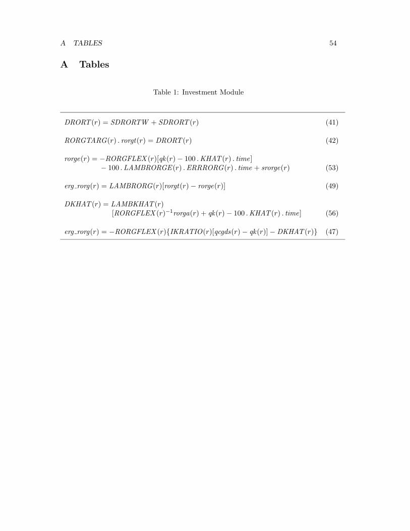
A Tables 54

B Figures 55

C Nomenclature 61

1 INTRODUCTION 1

1 Introduction

GTAP-Dyn is a recursively dynamic applied general equilibrium (AGE ) model of the

world economy. It extends the standard GTAP model (Hertel, 1997) to include inter-

national capital mobility, capital accumulation, and an adaptive expectations theory of

investment. This paper documents the extended theoretical structure.

Standard GTAP (Hertel and Tsigas, 1997) is a comparative-static AGE model of

the world economy, developed as a vehicle for teaching multi-country AGE modeling

and to complement the GTAP multi-country AGE data base (Gehlhar, Gray, Hertel et

al., 1997). In general, it aims to provide a straightforward presentation of widely used

AGE modeling techniques. It does however include some special features, notably an

extensive decomposition of welfare results.

The main objective of GTAP-Dyn is to provide a better treatment of the long run

within the GTAP framework. In standard GTAP, capital can move between industries

within a region, but not between regions. This impedes analysis of policy shocks and

other developments diversely affecting incentives to invest in different regions. For a

good long run treatment, then, we need international capital mobility.

With capital mobile between regions, we need to expand the national accounts

to allow for international income payments. Policies that attract capital to a region

may have a strong impact on gross domestic product; but, if the investment is funded

from abroad, the impact on gross national product and national income may be much

weaker. So, to avoid creating spurious links between investment and welfare, we need

to distinguish between asset ownership and asset location: the assets owned by a region

need no longer be the assets located in the region; the income generated by the assets

in a region need no longer accrue to that region’s residents.

To distinguish between asset location and ownership, we introduce a rudimentary

representation of financial assets. Regions now accumulate not only physical capital

stocks but also claims to the ownership of physical capital. These ownership claims are

financial assets of some kind. Thus international income receipts and payments emerge

as part of the system of accounting for financial assets.

With capital internationally mobile, we need to determine regional capital stocks.

This is most satisfactorily done in a dynamic model. First, tracing out the invest-

ment and capital stock time paths is the best way to assure ourselves that the end-

of-simulation capital stocks are reasonable. Second, the immediate impact of the

earlier-period investments required to achieve the end-of-simulation stocks on regional

economies is itself of some interest. Accordingly, we make the model dynamic, and in-

corporate the stock-flow or intrinsic dynamics of investment and capital accumulation.

1 INTRODUCTION 2

Likewise, we incorporate the intrinsic dynamics of saving and wealth accumulation.

Accordingly, the key features of this extension are endogenous regional capital

stocks, international assets and liabilities and international investment and income

flows, financial assets, and intrinsic dynamics of physical and financial asset stocks.

While introducing these new features we seek to preserve the strengths of the standard

model, including the ability to work with empirical rather than highly stylized data

bases, the ability to solve in reasonable time on reasonable computing platforms while

preserving a detailed regional and sectoral disaggregation, and a money metric of utility

and an associated decomposition.

The resultant model should be suitable for medium- and long-run policy analysis,

in which the comparative statics of the end-of-simulation solution is supplemented with

time paths leading to the solutions. It has enough dynamics and a sufficient treatment

of financial assets to support this, but not enough to support short-run macroeconomic

dynamics or financial or monetary economics.

This paper documents the theoretical structure of GTAP-Dyn as implemented in

the solution program. While we motivate each significant design decision, we do not

provide a tutorial introduction to the model, nor an academic treatment grounding

the model in the previous literature, but a technical reference. We intend to maintain

this document synchronously with the solution program, so that each revision of the

standard GTAP-Dyn solution program is accompanied by a corresponding revision of

this paper. This should ensure that a basic minimum level of documentation for the

theoretical structure is always available.

A salient technical feature of the new extension is the treatment of time. Many

dynamic models treat time as an index, so that each variable in the model has a time

index. In GTAP-Dyn, time itself is a variable, subject to exogenous change along

with the usual policy, technology, and demographic variables. Section 2 elucidates the

mechanics and motivation of this treatment, and section 3 applies it to the capital

accumulation equation. This lays the groundwork for the discussion in section 4 of

wealth accumulation, financial asset determination, and foreign income flows. Section 5

describes the investment theory, incorporating lagged adjustment of capital stocks and

adaptive expectations for the rate of return. Section 6 discusses the properties of the

complete model, the existence of and convergence toward a long-run equilibrium. The

paper concludes in section 7 with a summary of the strengths and limitations of the

new approach.

We provide a number of aids to the reader, to assist in following the notation and

in relating the paper to the solution program source code. We mark the definitions of

coefficients and variables by inserting their name as a marginal note. We provide a de-

2 TIME 3

scriptive listing of coefficients and variables appearing in the model code in appendix C.

We give each equation appearing in the model in two or three forms: the levels equation,

if appropriate, in mathematical notation, the differential (change) equation, in math-

ematical notation, and the differential equation, as coded in the model. The coded

equations are close but not literal transcriptions from the source code; since the layout

of the source code is still subject to revision, literal transcriptions are undesirable at

this time.

2 Time

As noted above (section 1), a key technical feature of GTAP-Dyn is the treatment of

time not as a discrete index but as a continuous variable. Since however the continu-

ous time treatment may be less familiar to many readers, we first overview the more

familiar discrete time approach, and then contrast the two. Within the vary large class

of dynamic economic models, we confine our discussion to recursively solvable CGE

models. In discussing solution methods, we assume the use of the GEMPACK suite of

economic modeling software.

We use a simplified wealth accumulation equation to illustrate and contrast the

two approaches. This equation combines features that might be separated between

the capital and wealth accumulation equations in a more complex model. It may not

correspond exactly to any accumulation equation in any working model, but it does,

we believe, support a fair presentation of features and issues typically encountered in

such models.

We consider a closed economy with a single capital good, which constitutes the sole

economic asset and hence the sole vehicle for saving. Real wealth may then be defined

as the size K of the capital stock. The evolution of the capital stock through time is

given by an integral equation,

K = K0 +

∫ T

T0

I(τ) dτ, (1)

where K0 denotes the capital stock at some base time T0, and I, net investment.

2.1 The discrete-time approach

Within a recursively solvable discrete-time framework, there is typically a concept of a

time period. A given data base refers to a given time period; a simulation takes the

data base to the next time period, with simulation results representing changes between

2 TIME 4

the initial period and the next.

Within such a framework, the database might include a representation of the econ-

omy in the current period, together with some extra data pertaining to the next period.

The representation of the economy might contain values as of the start of the period,

or as of the midpoint of the period, or average values over the period. The extra data

might be just the period length, or might include for example values of stocks at the

start of the next period.

Suppose that the data base contains a representation of the economy at the start of

the period, together with the period length. We have from equation (1), by the mean

value theorem, assuming a continuous time path for investment I,

K = K0 + (T − T0)I(Tm),

for some Tm between T0 and T , where we now interpret the base time T0 as the start of

the period represented by the initial data base. For small T−T0, we have I(Tm) ≈ I(T0),

so

K ≈ K0 + I0L, (2)

where L denotes the interval length T − T0. Differentiating, we obtain the percentage

change in the capital stock k within the simulation,

k ≈ 100I0L

K0.

We may calculate the right hand side as a formula outside the model, and apply it as

a shock to k; or, to avoid performing a separate calculation before the simulation, we

may include a capital accumulation equation within the solution program, writing

k ≈ 100I0L

K0h, (3)

where h is an artificial variable (sometimes called a homotopy variable) that is always

exogenous and always receives a shock of 1 in a dynamic simulation. Note that the

coefficients I0 and K0 refer to the start-of-simulation data base and are not updated

within the simulation.

We note that the change equation, equation (3), is true only approximately, not

exactly. This is not because of linearization error arising in the passage from the

levels to the change equation: indeed, there is no such error, since the levels equation,

equation (2), is itself linear. Instead, the change equation inherits error from the levels

equation, since the levels equation is itself inexact. Since the error is inherent in the

2 TIME 5

levels equation, it cannot be reduced by refinements in the solution procedure, such

as using smaller step sizes. The only way to reduce it is by revising the simulation

strategy, using more simulations with shorter time intervals. Once the time interval is

set, we have an irreducible inaccuracy in the accumulation equation.

At this point, readers familiar with the discrete time approach may object that

their own favorite discrete-time model does not suffer from this particular inaccuracy.

In general, however, it appears that it is possible to change the form of the inaccuracy,

but not to eliminate it. Suppose for example that the data base represents the average

state of the economy through the period, together with start-of-period and end-of-

period stocks. Then we can derive exact equations for the start-of-period and end-

of-period stocks for the next period, given initial-period and next-period investment.

To calculate the next-period average capital stock value, however, we need to know

how investment is distributed in time through the next period; but we cannot know

this. So the determination of the through-period-average capital stock is necessarily

approximate.

For sufficiently small time steps, this inaccuracy does not matter much; for larger

time steps, we must replace equation (3) by some other (more complex) equation that

offers a better approximation over longer periods. For example, in our closed economy

we may equate investment with saving; then we have I = S/Π, where S denotes nominal

net saving, and Π the price of investment goods. Then writing SAP for the average

propensity to save, we have S = SAPY and I = SAPY/Π, where Y denotes nominal

income; then writing Y as the product of real income YR and some price index PY , we

have

I =SAPPY YR

Π.

Substituting into equation (1), we have

K = K0 +

∫ T

T0

SAP (τ)PY (τ)YR(τ)

Π(τ)dτ. (4)

Now it is possible to solve equation (4) in terms of initial and final values of the

variables under the integral, only with the aid of various supplementary assumptions.

For example, one might assume that real income YR maintains some constant growth

rate between one period and the next; that the average propensity to consume, SAP ,

maintains some constant time rate of change; and that the prices PY and Π jump

immediately to their final values (prices being liable to overshooting, we might prefer

this to a steady growth assumption). The resulting equation would obviously be quite

different from (and far more complex than) equation (3). Less obviously, it will, like

2 TIME 6

that equation, include period-length-dependent parameters.

Thus by making assumptions about time paths of variables between adjacent pe-

riods, we might derive a longer-run wealth accumulation equation. The details of the

assumptions are not important; the point is that to implement the discrete-time ap-

proach for longer time intervals, we would need to make strong assumptions about

the time paths of various economic variables between time periods; that the variables

involved are typically endogenous to the system; and that the assumptions must be

applied not at run time but in developing the accumulation equation.

The method we have outlined is just one of many ways to implement a discrete time

treatment of capital accumulation, but it serves to illustrate some common features:

• The data base represents the economy in some period of time, possibly but not

necessarily at a single time point within the period.

• The capital accumulation equation includes coefficients derived not from the cur-

rent but from the start-of-simulation data base (it may also include some current

coefficients, though in our illustrative example it does not).

• The capital accumulation equation includes parameters that depend on the size

of the time step for the simulation (in our illustration, the time step size itself,

L).

• Given the size of the time step, there is some inaccuracy built into each experiment

that cannot be removed by refining the solution procedure.

• Major changes in the step size are liable to require revision not only of the pa-

rameters but also of the form of the capital accumulation equation.

• For longer time intervals, the accumulation equations are liable to embody strong

assumptions about time paths of endogenous variables.

In conclusion, the discrete time treatment of capital accumulation is perfectly viable,

but it is apt to suffer from some minor problems including inaccuracy, special assump-

tions about investment paths, and inflexibility in the size of the time step. Fortunately,

there is an alternative; capital accumulation lends itself naturally to a continuous time

approach, as we now describe.

2.2 The continuous-time approach

Returning to equation (1), we now reinterpret the data base as representing the economy

at some point in time. Both stock data and flow data refer to the same time point.

2 TIME 7

Also we treat T not as a discrete index but as a variable within the model. Totally

differentiating then, we obtain the equation

K = 100I

Kt, (5)

where k represents percentage change in the capital stock, and t, change in time. This

is very similar in form to the discrete-time equation (3). There are, however, two

differences: the time variable t replaces the homotopy variable h, and the equation uses

the current rather than initial values of investment I and the capital stock K.

These differences have major consequences. First, the new equation, being the

linearized form of equation (1), involves a linearization error, but not an irreducible

error. Thus the error in the calculation of the capital stock may be made as small as

desired by refining the solution procedure, for example, by increasing the number of

subintervals. Second, since there is no irreducible error, the equation is equally valid

for any time interval. Third, since the length of the time interval is given by a variable

(t) rather than by a parameter (L), the time interval length is determined at run time

rather than in the data base.

In contrast then to the discrete-time approach, our approach:

• uses the data base to represent the economy at a point in time,

• in a multi-step solution, uses no coefficients derived from the start-of-simulation

data base, but only current values,

• involves no parameters that depend on the length of the time interval,

• involves no irreducible inaccuracies in dynamic relations,

• uses the same accumulation equation for any time interval, and

• relies on no prior assumptions about the time paths of endogenous variables.

The notion of time as a variable can be explained in terms of the sources of change

in an economy. An economy may change not only in response to changes in external

circumstances such as technology, policy, or endowments, but also through the intrinsic

dynamics of its stock-flow relationships. In the presence of non-zero net investment

or saving, the passage of time leads to change in the stock of capital goods or of

wealth. Furthermore, with adaptive expectations or lagged adjustment, the passage of

time leads to the revision of expectations or the adjustment of target variables toward

equilibrium. Such changes, arising not from changes in external circumstances but

3 CAPITAL ACCUMULATION 8

autonomously through the passage of time, we capture in time terms (terms in the time

variable t) in the equation system. The shock to t defines the change in time through

the simulation; shocks to other exogenous variables represent accompanying changes in

external circumstances.

3 Capital accumulation

We now begin to apply the time treatment described in section 2 to the GTAP-Dyn

equation system. We begin with the capital accumulation equation, deriving the capital

stock variable used both in the investment theory (section 5) and in the financial assets

theory (section 4).

We begin with the integral equation for the capital stock,

QK = QK 0 +

∫ TIME

TIME 0QCGDSNET dτ, (6)

where QK (r) represents the capital stock in region r, QK 0 (r) the capital stock at QK

some base time TIME 0 , TIME , current time, and QCGDSNET (r), net investment.

Totally differentiating, we obtain

QK (r)qk(r)

100= QCGDSNET (r) . time, (7)

where qk(r) represents percentage change in the capital stock in region r, and time, qktime

change in time. Multiplying both sides by one hundred times the price of capital goods,

we obtain

VK (r) . qk(r) = 100NETINV (r) . time, (8)

where VK (r) denotes the money value of the capital stock in region r, and NETINV (r), VKNETINV

the money value of net investment.

In a static simulation, with time equal to zero, we see from equation (8) that the

percentage change in the capital stock qk is also zero. Sometimes however we wish

to impose some non-zero change in capital stocks. To that end we introduce into the

accumulation equation a region-generic shift factor SQKWORLD and a region-specific SQKWORLD

factor SQK (r). Incorporating those factors we obtain the final version of the levels SQK

equation,

QK (r) = SQKWORLD .SQK (r)

[

QKO(r) +

∫ TIME

TIME 0NETINV (r) dT

]

, (9)

4 FINANCIAL ASSETS AND ASSOCIATED INCOME FLOWS 9

the differential equation,

VK (r) . qk(r) = VK (r)[sqkworld + sqk(r)] + 100NETINV (r) . time, (10)

and the model code,

Equation E_qk #capital accumulation# (all,r,REG)

VK(r)*qk(r) = VK(r)*[sqkworld + sqk(r)] + 100*NETINV(r)*time;

4 Financial assets and associated income flows

As discussed in the introduction, to model international capital mobility we need to

distinguish between asset location and ownership; to do this, we introduce financial

assets. In GTAP-Dyn, regional households do not own physical capital; only firms

do. Households own not physical capital but financial assets, which represent indirect

claims on physical capital.

In this section, we show how the model determines agents’ financial assets and

liabilities, and the associated income receipts and payments. We begin with a dis-

cussion of the treatment’s general features (subsection 4.1) and a note on notation

(subsection 4.2). Stock-flow accumulation relations determine two key financial asset

variables (subsection 4.3); with those as constraints, we use an atheoretic mechanism to

determine the composition of firms’ liabilities and regional households’ assets (subsec-

tion 4.4). We complete the module with equations for the assets and liabilities of the

global financial intermediary (subsection 4.5) and income flows associated with financial

assets (subsection 4.6).

4.1 General features

Besides the prime motivation to take account of international capital mobility, several

other requirements have shaped the treatment of financial assets in GTAP-Dyn. For

reasons discussed below (section 5.1), we do not enforce rate-of-return equilibration

over the short run. This means that we need to represent gross ownership positions. It

is not enough, for example, to know a region’s net foreign assets; we must know both

its gross foreign assets and its gross foreign liabilities, since their rates of return may

differ.

To limit the burden of data construction for the extended model, and because data

on foreign assets and liabilities are limited and inconsistent, we prefer a treatment of

foreign assets that is parsimonious in its data requirements. We also want the treatment


to accommodate the salient empirical regularity of local specialization, that countries

do not hold globally balanced asset portfolios, but specialize strongly in holding local

assets.

We do not aim with the new treatment to give a full or accurate representation

of financial variables. The financial assets in GTAP-Dyn are there not to provide a

good representation of financial assets in the real world, but to let us represent inter-

national capital mobility without creating leaks in the foreign accounts. Our treatment

of financial assets accordingly is minimalist and highly stylized.

Influenced by these considerations, we determine some broad features of the financial

assets module. First and fundamentally, we elect not to adopt a full finance-theoretic

treatment of financial assets, but to take an ad hoc or heuristic approach. The attraction

of a finance-theoretic approach is that it would let us account in a principled way for

investors’ holding assets with different rates of return, rather than only the highest-

yielding asset. It would recognize that investors are concerned not only with return

but also with risk. It would relate their decisions on risk-return tradeoffs and their

consumption and saving behavior to the same set of underlying preferences, preserving

thereby the rigor of the welfare analysis.

On the other hand, introducing a finance-theoretic treatment would add greatly to

the complexity of the model, and yet create perhaps as many difficulties as it would

solve. There are a number of paradoxes in international financial behavior, empirical

regularities that are difficult to account for theoretically. Most relevantly here, it is dif-

ficult to account for observed disparities between countries in rates of return, which far

exceed those predicted with simple finance-theoretic models, plausible behavioral pa-

rameter settings, and observed risk levels. This does not rule out the finance-theoretic

approach, but it does make the cost-benefit balance less attractive. On balance then,

we elect not to implement such a treatment in this version of GTAP-Dyn, while ac-

knowledging its attractiveness as an area for future research.

After this basic decision, there are several further design decisions to make. First, we

must decide which physical assets should back financial assets; in other words, to which

assets should financial assets represent indirect claims. To allow for international capital

mobility, we must include physical capital in this set; we may also include primary

factors (endowment commodities in GTAP jargon) other than labor. In the standard

GTAP data base, at the time of writing (McDougall, Elbehri and Truong, 1998), these

are two: agricultural land, and other natural resources (mineral deposits, fisheries, and

forests). It would be more logical to let all these back financial assets, but it is easier

to let only physical capital back financial assets. In this version of the model, we take

the easier approach. Accordingly, in GTAP-Dyn, firms own physical capital, but rent


land and natural resources. Regional households, conversely, own land and natural

resources, which they lease to firms, and financial assets, which may be construed as

indirect claims on physical capital.

The next question is which classes of financial assets to represent in the model.

There are in the real world three broad classes of financial assets, money, debt, and

equity, divided in turn into many subclasses. Recognizing more asset classes would

potentially improve the realism of the model. On the other hand, for reasons discussed

above, realism in the representation of financial assets is not a priority for this model.

In light of this, and consistent with our stance that the role of the financial asset module

is to support international capital mobility rather than to depict the financial sector

realistically, we include in the model just one asset class, equity. Accordingly, in GTAP-

Dyn, firms have no liabilities, and only one asset, physical capital. By the fundamental

balance sheet identity (assets = liabilities + proprietorship), shareholder equity in the

firm is equal in value to the physical capital that the firm owns.

Next we ask which agents can hold equity in firms. The simplest design would be

to let all regional households hold equity in firms in all regions. This, however, would

require bilateral data on foreign assets and liabilities. Unfortunately the available data

are insufficient (pertaining mainly to foreign direct investment, not portfolio investment

or bond holdings) and internally inconsistent. To minimize the data requirements, we

adopt instead the fiction of a global trust that serves as a financial intermediary for all

foreign investment. Regional households, in GTAP-Dyn, do not hold equity directly in

foreign firms, but only in local firms and the global trust. The global trust in turn holds

equity in firms in all regions. The trust has no liabilities, and no assets other than its

equity in regional firms; so, by the balance sheet identity, total equity in the trust is

equal in value to total equity held by the trust.

A minor defect of this treatment is that it leads the model to misreport foreign

asset holdings. We identify each region’s equity in the global trust with its foreign

assets, when in fact some portion of it represents indirect ownership of local assets.

This misreporting is trivial for small regions, but more considerable for large regions

such as the United States.

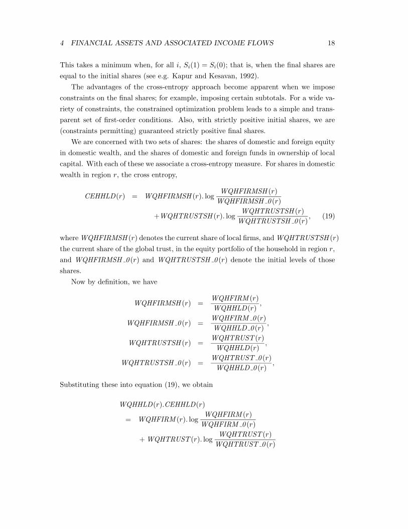
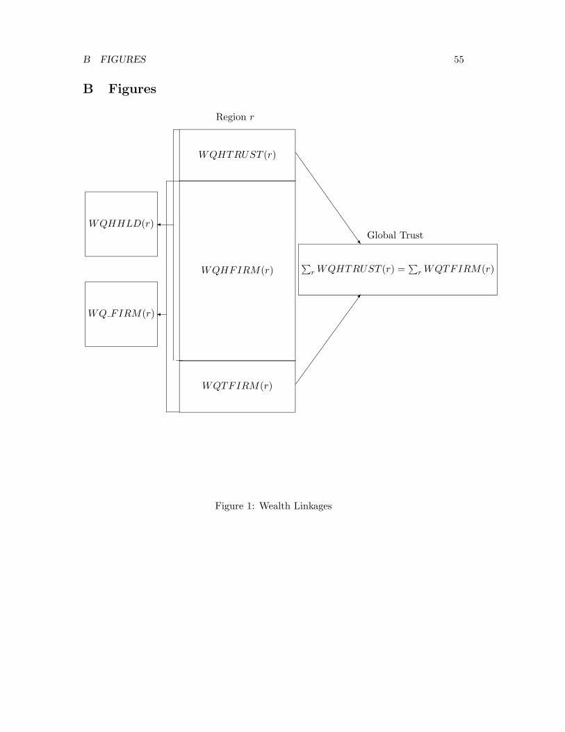
Figure 1 summarizes the financial asset framework. Firms in each region r have a

value WQ FIRM (r), of which the local regional household owns WQHFIRM (r) and

the global trust WQTFIRM (r). The global trust in turn is owned by the regional

households, each region r owning equity WQHTRUST (r). The total financial wealth

of the regional household comprises equity WQHFIRM (r) in local firms and equity

WQHTRUST (r) in the global trust. We discuss these relations further in subsections

4.3 and 4.5.


One further matter remains to be discussed, the concepts of income from and in-

vestment in physical and financial assets. We count as income the earnings of the asset,

but not capital gains or losses arising from asset price changes. For physical capital,

we also exclude physical depreciation from the definition of income (just as in standard

GTAP). For equity in firms or in the global trust, we count as investment the money

value of net change in the quantity of the entity’s assets, but exclude capital gains.

This treatment has two merits. First, it imposes consistency between income and

investment in financial assets: both exclude capital gains, so saving (calculated as total

investment in financial assets) is consistent with income. Second, it supports a simple

decomposition of change in proprietorship. Consider an entity that has no liabilities

but owns several assets. LetWAi denote the value of assets of type i, andW =∑

i WAi,

total asset value. Then percentage change w in total asset value is given by the equation

Ww =∑

i WAi(pAi + qAi), where pAi denotes percentage change in the price of asset i,

and qAi, percentage change in the quantity. We can use this equation to decompose

this change in total asset value into two components, the money value of net change in

the quantity of the entity’s assets, (1/100)∑

i WAiqAi, and the money value of change

in the prices of the quantity’s assets, (1/100)∑

i WAipAi.

Now by the balance sheet identity, total proprietorship in the firm is equal to total

asset value W , so w = pQ+ qQ, where pQ and qQ denote percentage change in the price

and volume of the firm’s stock. We can compose this into an investment component,

(1/100)WqQ, and a capital gain component, (1/100)WpQ. Then, by our conventional

definition of investment, WqQ =∑

i WAiqAi, so WpQ =∑

i WAipAi; that is, the price

of equity in the firm is proportional to an index of prices of the firm’s assets. Thus,

the price and quantity components of change in total proprietorship equate to the

corresponding components of change in total assets.

Another way to look at this is to imagine that firms and the trust fully distribute

their net earnings as dividends to shareholders, and fund their net asset purchases

entirely through new stock issues. Under this supposition, the value of dividends coin-

cides with the GTAP-Dyn definition of income, and the value of stock issues with the

GTAP-Dyn definition of financial investment.

4.2 Notation

To present this accounting framework we use a systematic notational convention. Per-

centage change variables are written in lower case; upper case variables are data co-

efficients, parameters, levels variables, or ordinary change variables. In general, the

first character of a variable or a coefficient shows its type: W (wealth) for asset values,


and Y for income flows. The second character identifies the asset type: in the current

version of the model, this is always Q for eQuity. The third character indicates the sec-

tor that owns the asset, or receives the income it generates, while the fourth character

identifies the sector that owes the asset, or pays the associated income. For example,

F designates investment in regional firms, T denotes investment in the global trust,

and H stands for investment by the regional household. Thus, a name beginning with

WQHF refers to the wealth in equity owned by the regional household and invested in

domestic firms, while a name beginning with YQHF refers to the income from equity

paid to the regional household by the domestic firms. An underscore is used in the

cases where the distinction pertaining to a particular character is not in point. The

underscore is left out if it is located at the end of the name.

4.3 Asset accumulation

The financial assets module revolves around two key variables: the ownership value of

firms in region r, and the equity holdings of the household in region r. Both these are

given, directly or indirectly, by accumulation relations.

In GTAP-Dyn, firms buy intermediate inputs, hire labor, and rent land, but own

fixed capital. They have no debt. In accounting terms they have no liabilities, and no

assets except fixed capital. Conversely, only firms own fixed capital. So the ownership

valueWQ FIRM (r) of firms in region r is equal to the value of their fixed capital, which WQ FIRM

is the value of all local fixed capital, which is equal to the product of the corresponding

price and quantity:

WQ FIRM (r) = VK (r) = PCGDS (r).QK (r),

where PCGDS (r) denotes the price of capital goods in region r. Differentiating, we PCGDS

obtain

wq f (r) = pcgds(r) + qk(r), (11)

where wq f (r) denotes percentage change in WQ FIRM (r), and pcgds(r), percentage wq fpcgds

change in PCGDS (r); in the model, we write

Equation REGEQYLCL #change in VK(r) [qk]# (all,r,REG)

wq_f(r) = pcgds(r) + qk(r);

Thus the total equity value of each region’s firms is given indirectly by the capital

accumulation equation, equation (10).

For future use we note that by the conventions discussed in section 4.1, the price

PQ FIRM (r) of equity in firms in region r is proportional to the price of capital goods


in region r,

pq f (r) = pcgds(r), (12)

where pq f denotes percentage change in PQ FIRM .

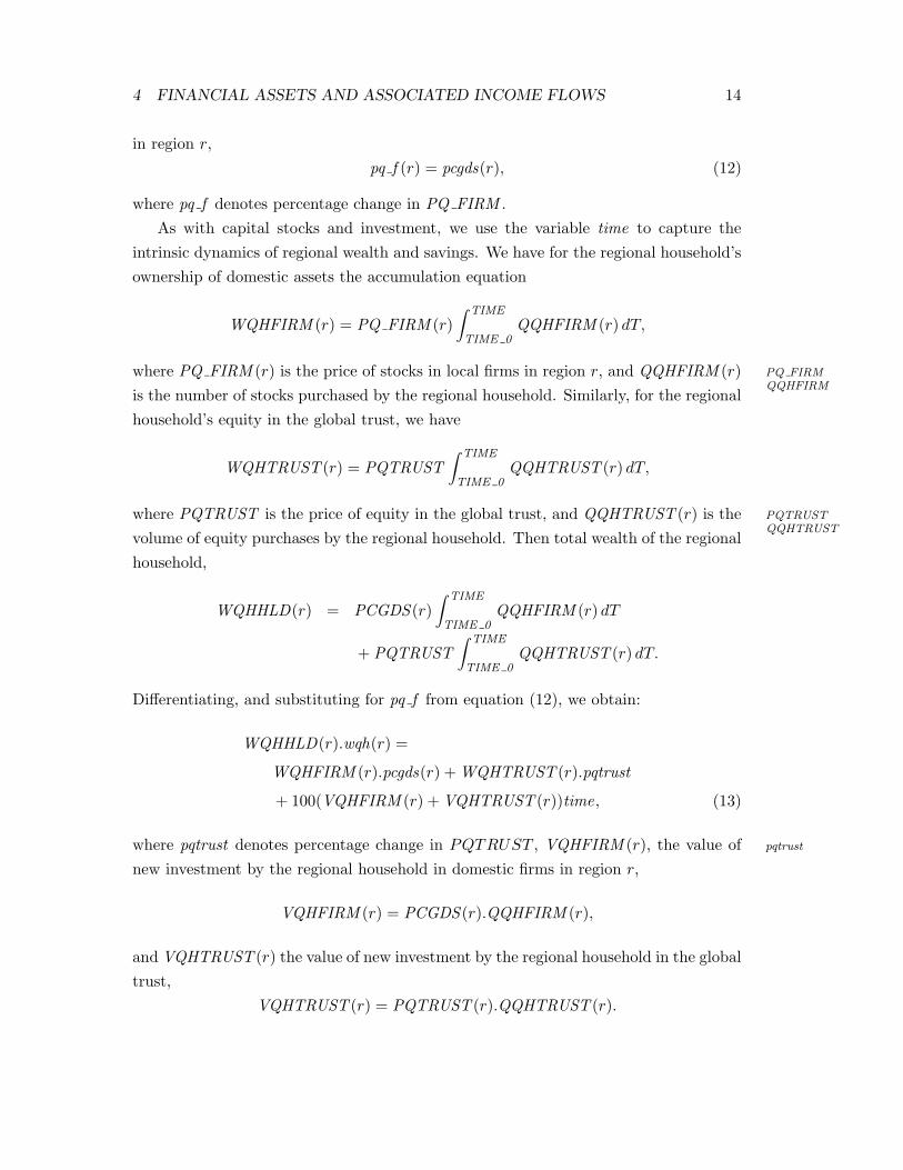
As with capital stocks and investment, we use the variable time to capture the

intrinsic dynamics of regional wealth and savings. We have for the regional household’s

ownership of domestic assets the accumulation equation

WQHFIRM (r) = PQ FIRM (r)

∫ TIME

TIME 0QQHFIRM (r) dT,

where PQ FIRM (r) is the price of stocks in local firms in region r, and QQHFIRM (r) PQ FIRMQQHFIRM

is the number of stocks purchased by the regional household. Similarly, for the regional

household’s equity in the global trust, we have

WQHTRUST (r) = PQTRUST

∫ TIME

TIME 0QQHTRUST (r) dT,

where PQTRUST is the price of equity in the global trust, and QQHTRUST (r) is the PQTRUSTQQHTRUST

volume of equity purchases by the regional household. Then total wealth of the regional

household,

WQHHLD(r) = PCGDS (r)

∫ TIME

TIME 0QQHFIRM (r) dT

+ PQTRUST

∫ TIME

TIME 0QQHTRUST (r) dT.

Differentiating, and substituting for pq f from equation (12), we obtain:

WQHHLD(r).wqh(r) =

WQHFIRM (r).pcgds(r) +WQHTRUST (r).pqtrust

+ 100(VQHFIRM (r) +VQHTRUST (r))time, (13)

where pqtrust denotes percentage change in PQTRUST , VQHFIRM (r), the value of pqtrust

new investment by the regional household in domestic firms in region r,

VQHFIRM (r) = PCGDS (r).QQHFIRM (r),

and VQHTRUST (r) the value of new investment by the regional household in the global

trust,

VQHTRUST (r) = PQTRUST (r).QQHTRUST (r).


Now total investment by the regional household in domestic and foreign equity is equal

to saving by the regional household— that is, VQHFIRM (r) + VQHTRUST (r) =

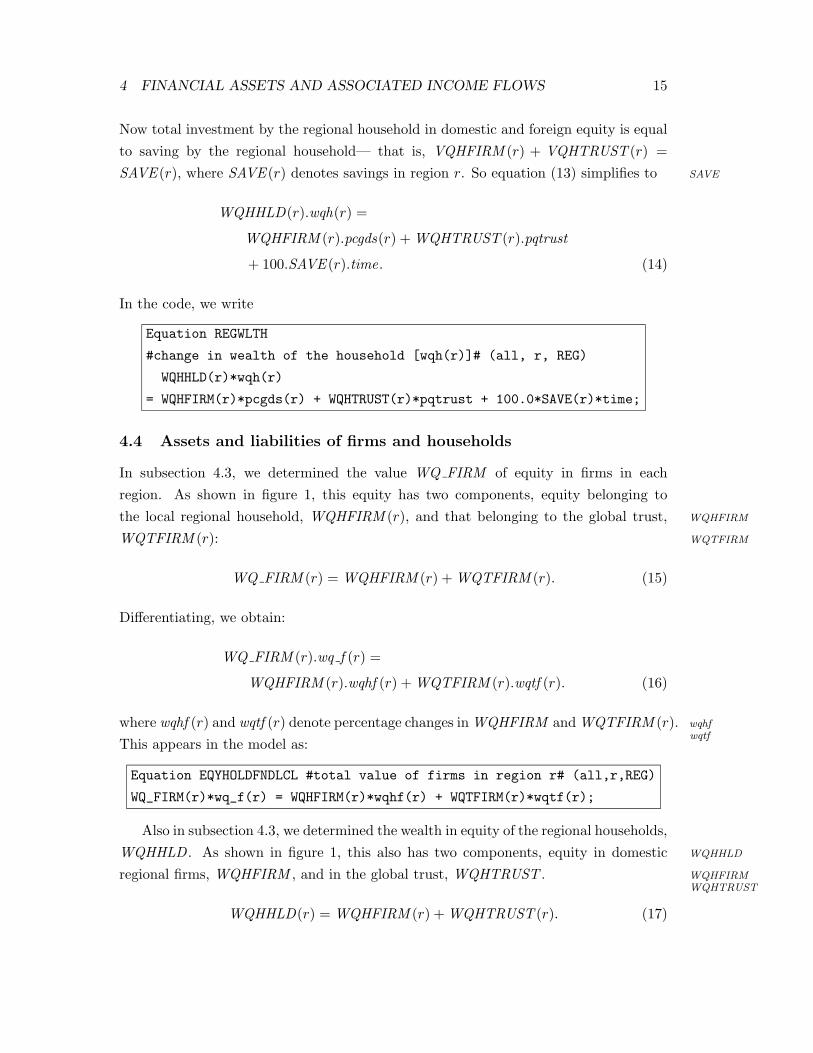
SAVE (r), where SAVE (r) denotes savings in region r. So equation (13) simplifies to SAVE

WQHHLD(r).wqh(r) =

WQHFIRM (r).pcgds(r) +WQHTRUST (r).pqtrust

+ 100.SAVE (r).time. (14)

In the code, we write

Equation REGWLTH

#change in wealth of the household [wqh(r)]# (all, r, REG)

WQHHLD(r)*wqh(r)

= WQHFIRM(r)*pcgds(r) + WQHTRUST(r)*pqtrust + 100.0*SAVE(r)*time;

4.4 Assets and liabilities of firms and households

In subsection 4.3, we determined the value WQ FIRM of equity in firms in each

region. As shown in figure 1, this equity has two components, equity belonging to

the local regional household, WQHFIRM (r), and that belonging to the global trust, WQHFIRM

WQTFIRM (r): WQTFIRM

WQ FIRM (r) =WQHFIRM (r) +WQTFIRM (r). (15)

Differentiating, we obtain:

WQ FIRM (r).wq f (r) =

WQHFIRM (r).wqhf (r) +WQTFIRM (r).wqtf (r). (16)

where wqhf (r) and wqtf (r) denote percentage changes inWQHFIRM andWQTFIRM (r). wqhfwqtf

This appears in the model as:

Equation EQYHOLDFNDLCL #total value of firms in region r# (all,r,REG)

WQ_FIRM(r)*wq_f(r) = WQHFIRM(r)*wqhf(r) + WQTFIRM(r)*wqtf(r);

Also in subsection 4.3, we determined the wealth in equity of the regional households,

WQHHLD . As shown in figure 1, this also has two components, equity in domestic WQHHLD

regional firms, WQHFIRM , and in the global trust, WQHTRUST . WQHFIRMWQHTRUST

WQHHLD(r) =WQHFIRM (r) +WQHTRUST (r). (17)


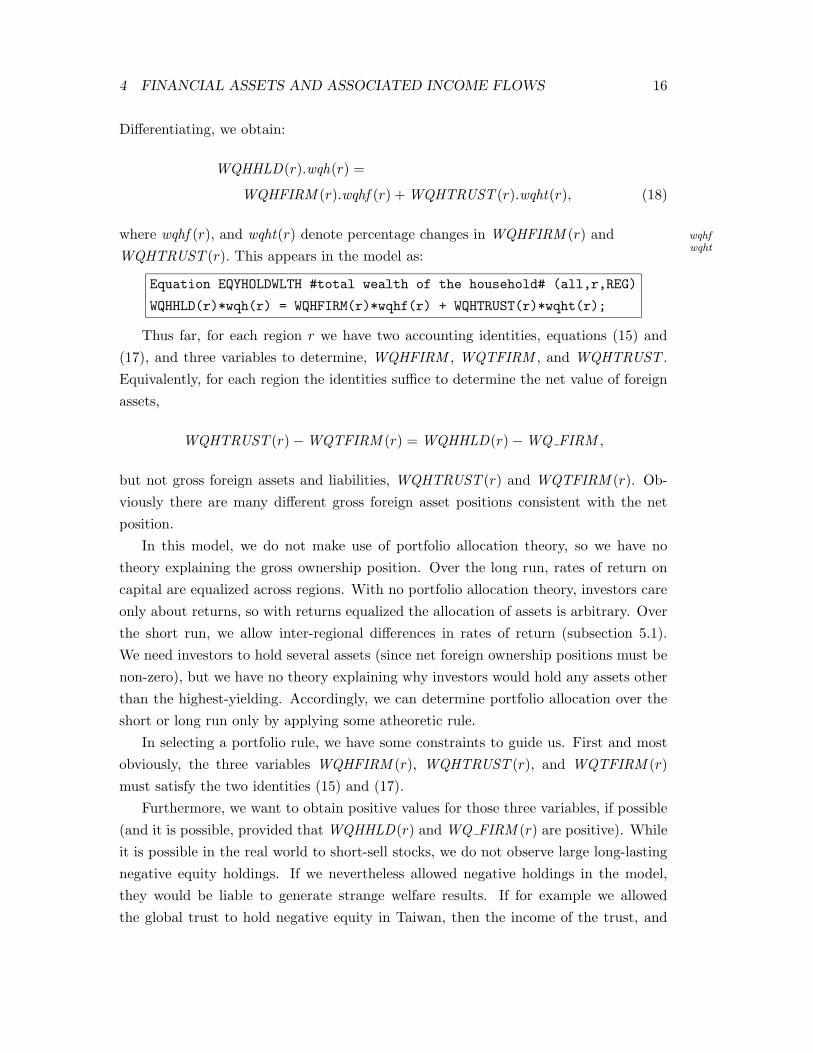
Differentiating, we obtain:

WQHHLD(r).wqh(r) =

WQHFIRM (r).wqhf (r) +WQHTRUST (r).wqht(r), (18)

where wqhf (r), and wqht(r) denote percentage changes in WQHFIRM (r) and wqhfwqht

WQHTRUST (r). This appears in the model as:

Equation EQYHOLDWLTH #total wealth of the household# (all,r,REG)

WQHHLD(r)*wqh(r) = WQHFIRM(r)*wqhf(r) + WQHTRUST(r)*wqht(r);

Thus far, for each region r we have two accounting identities, equations (15) and

(17), and three variables to determine, WQHFIRM , WQTFIRM , and WQHTRUST .

Equivalently, for each region the identities suffice to determine the net value of foreign

assets,

WQHTRUST (r)−WQTFIRM (r) =WQHHLD(r)−WQ FIRM ,

but not gross foreign assets and liabilities, WQHTRUST (r) and WQTFIRM (r). Ob-

viously there are many different gross foreign asset positions consistent with the net

position.

In this model, we do not make use of portfolio allocation theory, so we have no

theory explaining the gross ownership position. Over the long run, rates of return on

capital are equalized across regions. With no portfolio allocation theory, investors care

only about returns, so with returns equalized the allocation of assets is arbitrary. Over

the short run, we allow inter-regional differences in rates of return (subsection 5.1).

We need investors to hold several assets (since net foreign ownership positions must be

non-zero), but we have no theory explaining why investors would hold any assets other

than the highest-yielding. Accordingly, we can determine portfolio allocation over the

short or long run only by applying some atheoretic rule.

In selecting a portfolio rule, we have some constraints to guide us. First and most

obviously, the three variables WQHFIRM (r), WQHTRUST (r), and WQTFIRM (r)

must satisfy the two identities (15) and (17).

Furthermore, we want to obtain positive values for those three variables, if possible

(and it is possible, provided thatWQHHLD(r) andWQ FIRM (r) are positive). While

it is possible in the real world to short-sell stocks, we do not observe large long-lasting

negative equity holdings. If we nevertheless allowed negative holdings in the model,

they would be liable to generate strange welfare results. If for example we allowed

the global trust to hold negative equity in Taiwan, then the income of the trust, and


consequently, the foreign asset income of each region, would vary not directly but

inversely with Taiwanese capital rentals. Given the real-world absence of stable negative

equity holdings, this inverse relationship would be unrealistic.

Finally, we want the allocation rule to preserve as nearly as possible the initial

allocation of each region’s wealth between domestic and foreign assets. One of the

objectives of the asset treatment is to allow the model to respect the empirical regularity,

that regions tend to specialize their portfolios strongly in their own domestic assets. If

the initial data base respects this, we want updated data bases to respect it also.

One possible approach is to assume that each region allocated its wealth between

domestic and foreign assets in fixed proportions. This is simple and in some ways

appealing, but it has one defect: it makes it too easy for foreign liabilities to become

negative. A negative shock to productivity in Taiwan, for example, might cause the

value of capital located in Taiwan to fall more rapidly than the value of equity owned

by Taiwanese. With the fixed shares approach, the value of domestic equity owned

by Taiwanese might easily come to exceed the value of the Taiwanese capital stock, so

that the value of foreign ownership of Taiwanese industry would become negative. As

discussed above, we wish to avoid such outcomes.

If conversely we assumed that the composition of the source of funds was fixed

in each region, so that foreign and domestic equity in local capital varied in fixed

proportion, we would be assured that foreign ownership of local capital would not

turn negative; but growth in the local capital stock might easily lead to negative local

ownership of foreign assets.

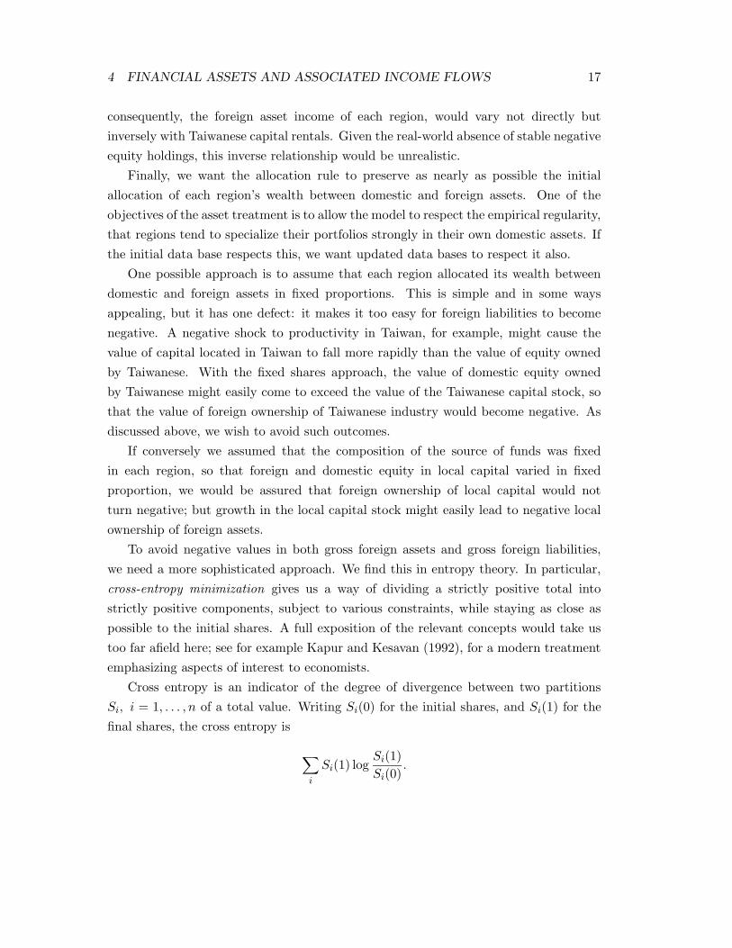
To avoid negative values in both gross foreign assets and gross foreign liabilities,

we need a more sophisticated approach. We find this in entropy theory. In particular,

cross-entropy minimization gives us a way of dividing a strictly positive total into

strictly positive components, subject to various constraints, while staying as close as

possible to the initial shares. A full exposition of the relevant concepts would take us

too far afield here; see for example Kapur and Kesavan (1992), for a modern treatment

emphasizing aspects of interest to economists.

Cross entropy is an indicator of the degree of divergence between two partitions

Si, i = 1, . . . , n of a total value. Writing Si(0) for the initial shares, and Si(1) for the

final shares, the cross entropy is

∑

i

Si(1) logSi(1)

Si(0).


This takes a minimum when, for all i, Si(1) = Si(0); that is, when the final shares are

equal to the initial shares (see e.g. Kapur and Kesavan, 1992).

The advantages of the cross-entropy approach become apparent when we impose

constraints on the final shares; for example, imposing certain subtotals. For a wide va-

riety of constraints, the constrained optimization problem leads to a simple and trans-

parent set of first-order conditions. Also, with strictly positive initial shares, we are

(constraints permitting) guaranteed strictly positive final shares.

We are concerned with two sets of shares: the shares of domestic and foreign equity

in domestic wealth, and the shares of domestic and foreign funds in ownership of local

capital. With each of these we associate a cross-entropy measure. For shares in domestic

wealth in region r, the cross entropy,

CEHHLD(r) = WQHFIRMSH (r). logWQHFIRMSH (r)

WQHFIRMSH 0 (r)

+WQHTRUSTSH (r). logWQHTRUSTSH (r)

WQHTRUSTSH 0 (r), (19)

whereWQHFIRMSH (r) denotes the current share of local firms, andWQHTRUSTSH (r)

the current share of the global trust, in the equity portfolio of the household in region r,

and WQHFIRMSH 0 (r) and WQHTRUSTSH 0 (r) denote the initial levels of those

shares.

Now by definition, we have

WQHFIRMSH (r) =WQHFIRM (r)

WQHHLD(r),

WQHFIRMSH 0 (r) =WQHFIRM 0 (r)

WQHHLD 0 (r),

WQHTRUSTSH (r) =WQHTRUST (r)

WQHHLD(r),

WQHTRUSTSH 0 (r) =WQHTRUST 0 (r)

WQHHLD 0 (r),

Substituting these into equation (19), we obtain

WQHHLD(r).CEHHLD(r)

= WQHFIRM (r). logWQHFIRM (r)

WQHFIRM 0 (r)

+WQHTRUST (r). logWQHTRUST (r)

WQHTRUST 0 (r)


−WQHHLD(r). logWQHHLD(r)

WQHHLD 0 (r).

Since WQHHLD(r) and WQHHLD 0 (r) are given, maximizing CEHHLD(r) is equiv-

alent to maximizing

FHHLD(r) = CEHHLD(r) +WQHHLD(r). logWQHHLD(r)

WQHHLD 0 (r).

Then

WQHHLD(r).FHHLD(r) =

WQHFIRM (r). logWQHFIRM (r)

WQHFIRM 0 (r)+WQHTRUST (r). log

WQHTRUST (r)

WQHTRUST 0 (r).

Similarly, maximizing the cross-entropy associated with the local capital ownership

shares is equivalent to maximizing FFIRM (r), where

WQ FIRM (r).FFIRM (r) =


WQHFIRM 0 (r)+WQTFIRM (r). log

WQTFIRM (r)

WQTFIRM 0 (r).

We seek to minimize a weighted sum of the two cross-entropies:

WSCE (r) = RIGWQH (r).WQHHLD(r).CEHHLD(r)

+ RIGWQ F (r).WQ FIRM (r).CEFIRM (r).

The two cross-entropies are weighted by the corresponding total values, WQHHLD(r)

and WQ FIRM (r), and explicitly by the rigidity parameters RIGWQH (r) and RIGWQH

RIGWQ F (r). If RIGWQH (r) is assigned a high value, and RIGWQ F (r) a low one, RIGWQ F

then the solution will, if possible, keep the allocation of household wealth nearly fixed,

and put most of the onus of adjustment on the source shares for equity in local firms. If

RIGWQ F (r) is assigned a high value, and RIGWQH (r) a low one, the equity source

shares will tend to remain near their initial values, and the household wealth allocation

shares do most of the adjusting.

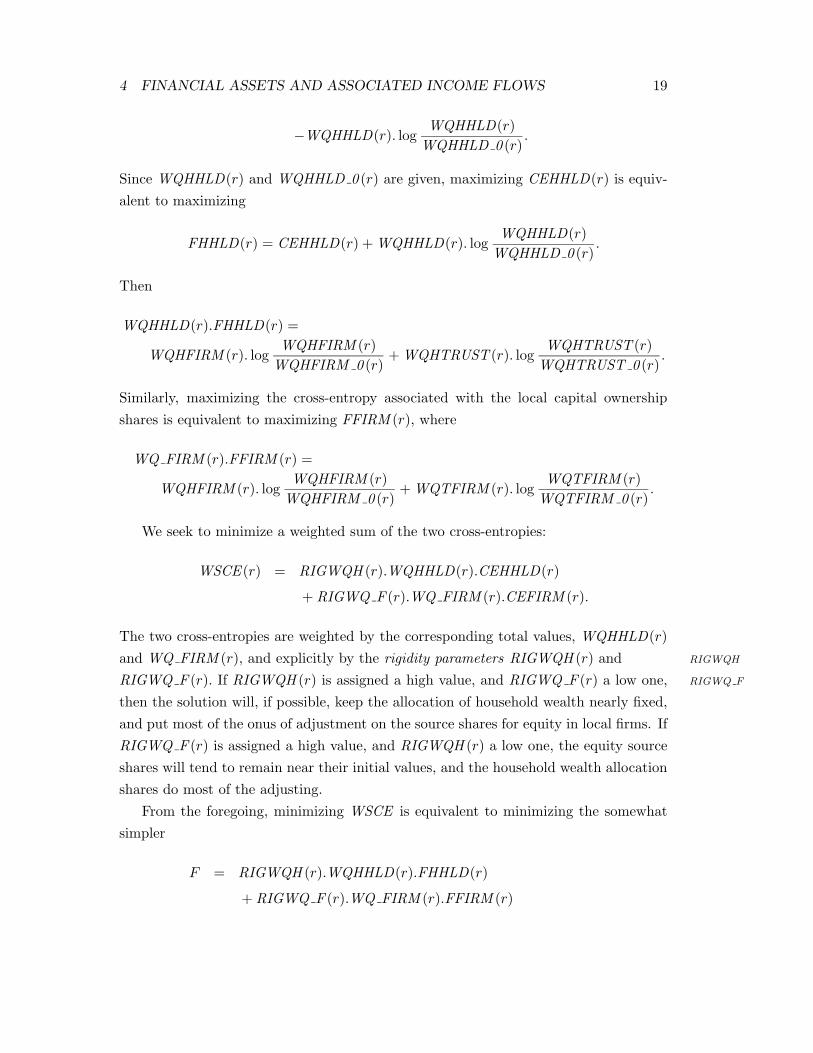
From the foregoing, minimizing WSCE is equivalent to minimizing the somewhat

simpler

F = RIGWQH (r).WQHHLD(r).FHHLD(r)

+ RIGWQ F (r).WQ FIRM (r).FFIRM (r)


= RIGWQH (r)

(


WQHFIRM 0 (r)

+WQHTRUST (r). logWQHTRUST (r)

WQHTRUST 0 (r)

)

+ RIGWQ F (r)

(


WQHFIRM 0 (r)

+WQTFIRM (r). logWQTFIRM (r)

WQTFIRM 0 (r)

)

.

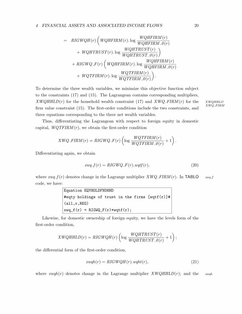
To determine the three wealth variables, we minimize this objective function subject

to the constraints (17) and (15). The Lagrangean contains corresponding multipliers,

XWQHHLD(r) for the household wealth constraint (17) and XWQ FIRM (r) for the XWQHHLDXWQ FIRM

firm value constraint (15). The first-order conditions include the two constraints, and

three equations corresponding to the three net wealth variables.

Thus, differentiating the Lagrangean with respect to foreign equity in domestic

capital, WQTFIRM (r), we obtain the first-order condition

XWQ FIRM (r) = RIGWQ F (r)

(

logWQTFIRM (r)

WQTFIRM 0 (r)+ 1

)

.

Differentiating again, we obtain

xwq f (r) = RIGWQ F (r).wqtf (r), (20)

where xwq f (r) denotes change in the Lagrange multiplier XWQ FIRM (r). In TABLO xwq f

code, we have:

Equation EQYHOLDFNDHHD

#eqty holdings of trust in the firms [wqtf(r)]#

(all,r,REG)

xwq_f(r) = RIGWQ_F(r)*wqtf(r);

Likewise, for domestic ownership of foreign equity, we have the levels form of the

first-order condition,

XWQHHLD(r) = RIGWQH (r)

(

logWQHTRUST (r)

WQHTRUST 0 (r)+ 1

)

;

the differential form of the first-order condition,

xwqh(r) = RIGWQH (r).wqht(r), (21)

where xwqh(r) denotes change in the Lagrange multiplier XWQHHLD(r); and the xwqh


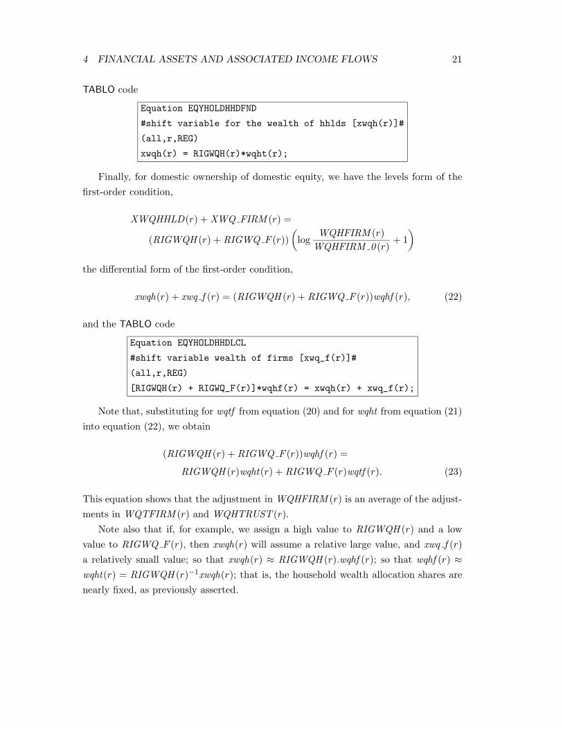
TABLO code

Equation EQYHOLDHHDFND

#shift variable for the wealth of hhlds [xwqh(r)]#

(all,r,REG)

xwqh(r) = RIGWQH(r)*wqht(r);

Finally, for domestic ownership of domestic equity, we have the levels form of the

first-order condition,

XWQHHLD(r) +XWQ FIRM (r) =

(RIGWQH (r) + RIGWQ F (r))

(

logWQHFIRM (r)

WQHFIRM 0 (r)+ 1

)

the differential form of the first-order condition,

xwqh(r) + xwq f (r) = (RIGWQH (r) + RIGWQ F (r))wqhf (r), (22)

and the TABLO code

Equation EQYHOLDHHDLCL

#shift variable wealth of firms [xwq_f(r)]#

(all,r,REG)

[RIGWQH(r) + RIGWQ_F(r)]*wqhf(r) = xwqh(r) + xwq_f(r);

Note that, substituting for wqtf from equation (20) and for wqht from equation (21)

into equation (22), we obtain

(RIGWQH (r) + RIGWQ F (r))wqhf (r) =

RIGWQH (r)wqht(r) + RIGWQ F (r)wqtf (r). (23)

This equation shows that the adjustment inWQHFIRM (r) is an average of the adjust-

ments in WQTFIRM (r) and WQHTRUST (r).

Note also that if, for example, we assign a high value to RIGWQH (r) and a low

value to RIGWQ F (r), then xwqh(r) will assume a relative large value, and xwq f (r)

a relatively small value; so that xwqh(r) ≈ RIGWQH (r).wqhf (r); so that wqhf (r) ≈

wqht(r) = RIGWQH (r)−1xwqh(r); that is, the household wealth allocation shares are

nearly fixed, as previously asserted.


4.5 Assets and liabilities of the global trust

There are three accounting identities associated with the global trust. First, the value

of assets owned by the global trust, WQTRUST , is equal to the sum across regions of WQTRUST

foreign ownership of firms:

WQTRUST =∑

r

WQTFIRM (r); (24)

In percentage change form, we have:

WQTRUST .wqt =∑

r

WQTFIRM (r).wqtf (r), (25)

where wqt is the percentage change in WQTRUST ; in the TABLO code: wqt

Equation TOTGFNDASSETS #value of assets owned by global trust#

WQTRUST*wqt = sum{s, REG, WQTFIRM(s)*wqtf(s)};

The second identity is that the value of the trust, WQ TRUST , is equal to the sum WQ TRUST

of the regions’ equity in the trust, that is, to the sum across regions of ownership of

foreign assets:

WQ TRUST =∑

r

WQHTRUST (r); (26)

In percentage change form,

WQ TRUST .wq t =∑

r

WQHTRUST (r).wqht(r),

where wq t is the percentage change in WQ TRUST ; in the TABLO code, wq t

Equation TOTGFNDPROP #value of trust as total ownership of trust#

WQ_TRUST*wq_t = sum{s, REG, WQHTRUST(s)*wqht(s)};

Finally, the total value of the trust is equal to the total value of its assets:

WQ TRUST =WQTRUST .

This equation as written would be redundant in the model, since it is implicit in other

relations. The accumulation equations, together with the equivalence of global invest-

ment and global saving, ensure that the total value of physical capital is always equal

to the total value of financial asset ownership by regions: so

∑

r

WQ FIRM (r) =∑

r

WQHHLD(r). (27)


Then

WQ TRUST =∑

r

WQHTRUST (r) by equation (26)

=∑

r

(WQHHLD(r)−WQHFIRM (r)) by equation (15)

=∑

r

WQHHLD(r)−∑

r

WQHFIRM (r)

=∑

r

WQ FIRM (r)−∑

r

WQHFIRM (r) by equation (27)

=∑

r

(WQ FIRM (r)−WQHFIRM (r))

=∑

r

WQTFIRM (r) by equation (17)

= WQTRUST by equation (24),

as was to be shown.

To verify that simulation results satisfy the identity, we include in the model the

equation

WQTRUST =WTRUSTSLACK .WQ TRUST ,

where WTRUSTSLACK denotes an endogenous slack variable. In percentage change WTRUSTSLACK

form,

wqt = wq t + wtrustslack , (28)

where wtrustslack denotes percentage change inWTRUSTSLACK . In the TABLO code, wtrustslack

Equation GLOB_BLNC_SHEET

#check that ownership by the trust equals ownership of the trust#

wqt = wq_t + wtrustslack;

Provided that the model data base respects the asset accounting identities (and assum-

ing no errors in the equations), the variable wtrustslack is endogenously equal to zero

in any simulation. Thus the result for the slack variable provides a check on the validity

of the model. Figure 1 illustrates these accounting relations.

Corresponding to equation (25) for asset values we have a price equation. As dis-

cussed in section 4.1, we can divide growth in assets and in proprietorship into matching

investment and capital gain components. For the global trust, equating the capital gain

components of assets and proprietorship yields the equation

pqtrust =∑

r

WQTFIRM (r)

WQTRUSTpcgds(r)


=∑

r

WQT FIRMSHR(r).pcgds(r), (29)

where WQT FIRMSHR(r) denotes the share of region r equities in total assets of the WQT FIRMSHR

global trust. In the code, this becomes

Equation PKWRLD

#change in the price of equity in the global fund#

pqtrust = sum{r, REG, WQT_FIRMSHR(r)*pcgds(r)};

4.6 Income from financial assets

Having determined stocks of financial assets in the foregoing subsections, we now de-

termine the associated income flows. We do this in three stages. First, we determine

payments from firms to households and to the global trust. Second, we calculate the

total income of the global trust, and determine payments from the trust to regional

households. Third, we calculate the equity income of regional households as the sum of

receipts from local firms and from the global trust.

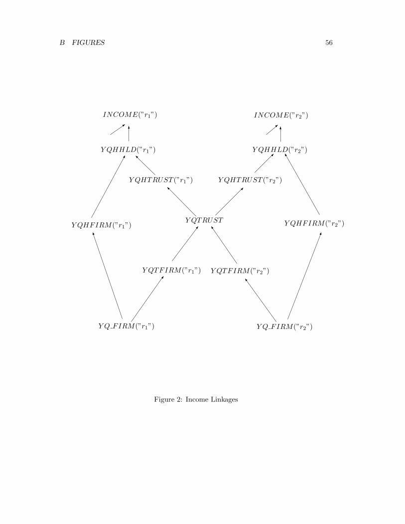
For an overview of the equity income flows, we refer to figure 2. Firms in region r dis-

tribute to shareholders equity income payments YQ FIRM (r), of which YQHFIRM (r)

goes to the local regional household and YQTFIRM (r) to the global trust. Summing

these receipts YQTFIRM (r) across regions, we obtain the total income YQTRUST

of the global trust. The trust distributes this amongst the regional households, with

region r receiving an amount YQHTRUST (r). Thus the total equity income of re-

gion r, YQHHLD(r), is the sum of receipts YQHFIRM (r) from local firms and receipts

YQHTRUST (r) from the global trust. This summed with non-equity factor income

and indirect taxes yields total regional income INCOME (r).

We begin the detailed discussion with payments by firms. Firms buy intermediate

inputs, hire labor, and rent land, but own fixed capital. By the zero pure profits

condition, their profits are equal to the cost of capital services, excluding any factor

usage or income taxes, less depreciation. These profits accrue to shareholders. Thus

total income payments by firms in region r to shareholders, YQ FIRM (r), are equal to YQ FIRM

net after-tax capital earnings:

YQ FIRM (r) = VOA(“capital”, r)−VDEP(r),

where VOA(“capital”, r) is the value of capital earnings, and VDEP(r) is the value of VOAVDEP

capital depreciation. Differentiating, we obtain

YQ FIRM (r)yq f (r) =


VOA(“capital”, r)(rental(r) + qk(r))−VDEP(r)(pcgds(r) + qk(r)),

where yq f (r) denotes the percentage change in income payments by firms in region r, yq f

and rental(r), percentage change in the rental price of capital. In the code, this becomes rental

(somewhat obscurely)

Equation REGINCEQY #income from capital in firms in region r#

(all, r, REG)

YQ_FIRM(r)*yq_f(r)

= sum{h, ENDWC_COMM, VOA(h,r)*[ps(h,r) + qo(h,r)]}

- VDEP(r)*[pcgds(r) + qk(r)];

To relate this to the mathematical form of the equation, note that ENDWC_COMM

is a set with just one element, "capital", with ps(“capital”, r) = rental(r) and

qo(“capital”, r) = qk(r).

Firms distribute payments amongst shareholders in proportion to their sharehold-

ings. The local regional household owns WQHFIRM and the global trust WQTFIRM

of a total equity valueWQ FIRM (see subsection 4.4). So for payments YQHFIRM (r) YQHFIRM

to the local regional household, we have

YQHFIRM (r) =WQHFIRM (r)

WQ FIRM (r)YQ FIRM (r). (30)

Differentiating, we obtain

yqhf (r) = yq f (r) + wqhf (r)− wq f (r); (31)

where yqhf (r) denotes the percentage change in YQHFIRM (r). In the TABLO code, yqhf

Equation INCHHDLCLEQY

#income of the household from dom firms [yqhf(r)]# (all,r,REG)

yqhf(r) = yq_f(r) + wqhf(r) - wq_f(r);

Similarly, payments to the global trust, YQTFIRM (r), are given by YQTFIRM

YQTFIRM (r) =WQTFIRM (r)

WQ FIRM (r)YQ FIRM (r), (32)


yqtf (r) = yq f (r) + wqtf (r)− wq f (r), (33)

where yqtf (r) is the percentage change in YQTFIRM (r). In the model, we write yqtf


Equation INCFNDLCLEQY #income of trust from equity in firms r#

(all, r, REG)

yqtf(r) = yq_f(r) + wqtf(r) - wq_f(r);

In the second stage we compute total income receipts and the various income pay-

ments of the global trust. The total income of the trust, YQTRUST , is equal to the YQTRUST

sum of equity receipts from firms in each region. In levels, we express this as:

YQTRUST =∑

r

YQTFIRM (r);

in percentage changes, as:

yqt =∑

r

YQTFIRM (r)

YQTRUSTyqtf (r),

where yqt denotes the percentage change in YQTRUST ; and in the TABLO code, as: yqt

Equation INCFNDEQY

#change in the income of the trust#

yqt = sum{r, REG, [YQTFIRM(r)/YQTRUST]*yqtf(r)};

The trust distributes its income amongst its shareholders, so that each region r

receives income YQHTRUST (r) in proportion to its ownership share. This is expressed YQHTRUST

in the levels equation

YQHTRUST (r) =WQHTRUST (r)

WQ TRUSTYQTRUST ;

the differential equation

yqht(r) = yqt + wqht(r)− wq t , (34)

where yqht(r) denotes the percentage change in YQHTRUST ; and in the TABLO code yqht

Equation REGGLBANK #income of hhld r from its shrs in the trust#

(all,r,REG)

yqht(r) = yqt + wqht(r) - wq_t;

In the third and final stage we compute the financial asset income of regional house-

holds. Total equity income YQHHLD(r) of regional household r equals the sum of YQHHLD

equity income received from domestic firms and from the global trust:

YQHHLD(r) = YQHFIRM (r) +YQHTRUST (r).

5 INVESTMENT THEORY 27

In percentage changes,

yqh(r) =YQHFIRM (r)

YQHHLD(r)yqhf (r) +

YQHTRUST (r)

YQHHLD(r)yqht(r), (35)

where yqh(r) denotes percentage change in YQHHLD ; in the TABLO code, yqh

Equation TOTINCEQY #total income from equity of households in r#

(all,r,REG)

yqh(r)

= [YQHFIRM(r)/YQHHLD(r)]*yqhf(r) + [YQHTRUST(r)/YQHHLD(r)]*yqht(r);

5 Investment Theory

In this section we describe a lagged adjustment, adaptive expectations theory of in-

vestment. Investors act so as to eliminate disparities in expected rates of return not

instantaneously, but progressively through time. Moreover, their expectations of rates

of return may be in error, and these errors are also corrected progressively through

time. Finally, in estimating future rates of return, they allow for some normal rate of

growth in the capital stock; and this normal rate too is an estimated rate that investors

adjust through time.

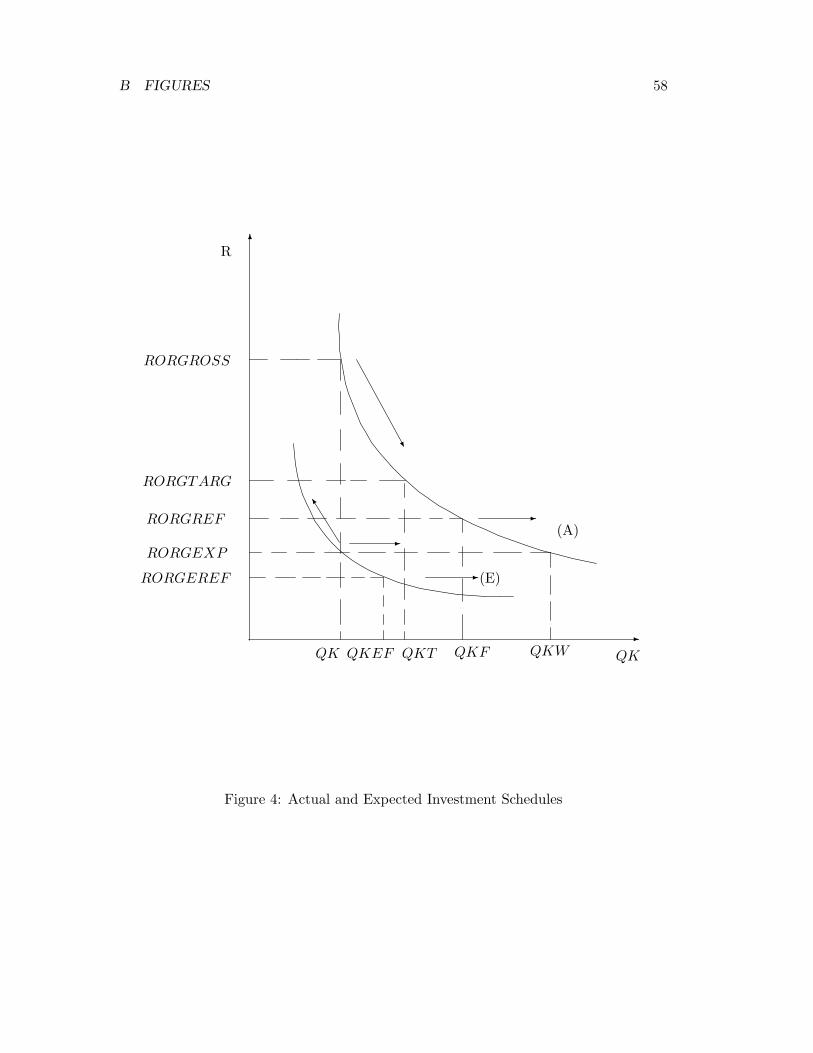
5.1 The required rate of growth in the rate of return

In a simple perfect adjustment model of investment, profit-maximizing investors would

keep rates of return uniform across regions, since any differences in rates of return

would be immediately eliminated by a reallocation of capital from regions with lower

rates of return to regions with higher rates. This equalization would apply to net rates

of return, so that we might write, for each region r, RORNET (r) = RORCOMM , where

RORNET (r) denotes the net rate of return on capital in region r, and RORCOMM

the common world rate of return.

If we allow for region specific risk premia RRISK (r), then we postulate equaliza-

tion not of the actual net rates of return RORNET (r) but of the risk-adjusted rates

RORNET (r) − RRISK (r), so that, for all regions r, RORNET (r) = RORCOMM +

RRISK (r). Furthermore, as we find below, it is convenient to express the investment

theory in terms of gross rather than net rates of return; anticipating this, we write

RDEP(r) for the depreciation rate in region r, and obtain for the gross rate of return


the equilibrium condition

RORGROSS (r)− RORCOMM − RRISK (r)− RDEP(r) = 0. (36)

In principle, the gross rate of return RORGROSS (r) includes both an earnings RORGROSS

component and a capital gains component:

RORGROSS (r) =RENTAL(r)

PCGDS (r)+ RG PCGDS (r), (37)

where RENTAL(r) denotes the rental price of capital in region r and RG PCGDS (r), RENTAL

the rate of growth in the purchase price of capital. In practice, with a period-by-period

solution method, we do not know the rate of growth in the purchase price of capital,1

so we neglect it and define the gross rate of return as the earnings rate only:

RORGROSS (r) =RENTAL(r)

PCGDS (r).

Differentiating, we obtain the percentage change equation

rorga(r) = rental(r)− pcgds(r), (38)

where rorga(r) denotes percentage change in RORGROSS ; and the model code rorga

Equation E_rorga #identity for rate of return# (all,r,REG)

rorga(r) = rental(r) - pcgds(r);

We now consider investment response to sudden (that is, instantaneous) price

changes. Sudden price changes may occur, for example, as the result of sudden tax

rate changes. Sudden changes to output or input prices affect the capital rental price

RENTAL(r), and thereby the rate of return. In a perfect adjustment model with capital

gains, they must be offset by some sudden change in PCGDS or RG PCGDS , or by

some sudden offsetting influence on RENTAL, so as to maintain international equality

in rates of return as defined in equation (37).

Suppose initially that the supply of capital goods is perfectly elastic. Then a first-

round improvement in profitability, that is, a first round positive effect on RENTAL,

leads to an increase in the capital stock, increasing output supply (and possibly in-

creasing demand for non-capital inputs) and thereby negating the first-round effect on1In fact, we can estimate the backward-looking growth rate, limH→0−(PCGDS(r;T + H) −

PCGDS(r;T ))/H, where PCGDS(r;x) denotes the value of PCGDS(r) at time T . This however isliable to differ from the forward looking growth rate, limH→0+(PCGDS(r;T +H)−PCGDS(r;T ))/H,which is the one needed in the rate of return formula.


RENTAL. If the initial shock is sudden, then so also must be the increase in the capital

stock; this implies an infinite rate of investment over an infinitesimal time period.

In the real world of course capital stocks do not adjust in this manner. Instantaneous

adjustment of capital stocks is precluded by gestation lags, adjustment costs, imperfect

elasticity of supply of capital, etc. In a CGE model also, even if other realistic features

are lacking, the supply of capital is typically imperfectly elastic.

If we rule out infinite rates of investment, how can rate of return equalization be

maintained in the face of sudden shocks affecting profitability? The answer is through

sudden changes in the price of capital goods. A sudden improvement in earnings leads

to a sudden increase in demand for capital goods, and that in turn to a sudden increase

in the price of capital goods. This helps to stabilize the rate of return in two ways. First,

it reduces the earnings rate RENTAL(r)/PCGDS (R). Second, it leads to a decrease in

the rate of capital gain RG PCGDS : as demand for capital goods eases through time

after the initial spike, or the supply of capital goods gradually rises, the price of capital

goods tends to fall through time after its initial increase.

In our model, we cannot capture the capital gains effect of an increase in demand

for capital goods, but we can capture the earnings rate effect. Thus the way appears

open in principle to use a perfect adjustment mechanism for investment. Since we do

not capture all the effects of the increase in demand for capital, however, it is likely

that the model will require unrealistically large increases in the price of capital goods

and in the level of investment.

Indeed, there are several reasons why the model would tend to exaggerate investment

volatility, some already mentioned, some not:

• The model does not capture the capital gain effect of capital goods price changes.

• As we typically use it in dynamic simulations, the model assumes perfect capital

mobility within regions. Accordingly, it overstates the elasticity of supply of

capital goods.

• The model does not incorporate other real-world effects such as gestation lags or

adjustment costs.

For all these reasons, the perfect adjustment approach is unrealistic in the con-

text of this model. We pursue accordingly a lagged adjustment approach. Recalling

equation (36), we rewrite it as

RORGROSS (r)− RORGTARG(r) = 0,


where RORGTARG(r) denotes the target rate of return in region r. To move to a RORGTARG

lagged adjustment approach, we replace this in turn by

RRG RORG(r) = LAMBRORG(r) ∗ logRORGTARG(r)

RORGROSS (r), (39)

where RRG RORG(r) denotes the required rate of growth in the rate of return, and RRG RORG

LAMBRORG(r) a coefficient of adjustment. Differentiating, we obtain LAMBRORG

rrg rorg(r) = LAMBRORG(r) ∗ [rorgt(r)− rorga(r)], (40)

where rrg rorg(r) denotes (absolute) change in the required rate of growth in the rate rrg rorg

of return in region r, and rorgt(r), percentage change in the target rate of return. Note rorgt

that this is not the final form of the equation; we present that in subsection 5.3 below,

following further theoretical development.

Referring back to equation (36), we note that the target rate of return includes both

region-specific components RRISK (r) and RDEP(r) and a region-generic component

RORCOMM . In the present context there is a further possible region-generic com-

ponent, a world-wide drift in rates of return such as to accommodate the global level

of investment. We do not represent all these components explicitly in the model, but

instead write simply

RORGTARG(r) = SDRORTWORLD + SDRORTARG(r),

where SDRORTWORLD denotes a region-generic component in the target rate of re- SDRORTWORLD

turn, and SDRORTARG(r) a component specific to region r. Differentiating, we obtain SDRORTARG

DRORT (r) = SDRORTW + SDRORT (r),

where DRORT (r) denotes the absolute change in the target rate of return, SDRORTW DRORTSDRORTW

a region-generic shift, and SDRORT (r) a region-specific shift. We use here the abso- SDRORT

lute rather than the percentage change form for the target rate, to ensure that any

world-wide shift SDRORTW leads to equal percentage-point changes in rates of return

in different regions; equivalently, to ensure that any cross-region differentials are main-

tained in percentage point rather than percentage terms (so, for example, we might

maintain a risk premium of two percentage points, but not a risk premium equivalent

to 20 per cent of the rate of return). We have then

DRORT (r) = SDRORTW + SDRORT (r); (41)


or in TABLO code,

Equation E_DRORT #equilibrium condition for rate of return#

(all,r,REG)

DRORT(r) = SDRORTW + SDRORT(r);

We relate the absolute-change variable DRORT to the percentage-change variable

rorgt with the equation

RORGTARG(r).rorgt(r) = DRORT (r); (42)

in the code,

Equation E_rorgt #identity for target gross rate of return#

(all,r,REG)

RORGTARG(r)*rorgt(r) = DRORT(r);

5.2 The expected rate of growth in the rate of return

Having determined above (subsection 5.1) the required rate of growth in the rate of

return, we now relate this to the level of investment, through an equation linking the

expected rate of growth in the rate of return to investment, and a condition that the

expected rate should be equal to the required rate.

This brings us to one of the central elements of the investment theory, the expected

rate of return schedule. Investors understand that, the higher the level of the capital

stock at any given time, the lower the rate of return at that time. Accordingly, the rate

of return expected to prevail at any future time depends on the capital stock at that

time. Consequently, the expected rate of growth in the rate of return depends on the

rate of growth in the capital stock; or, equivalently, on the level of investment.

We describe investors’ understanding of the investment environment through a rate

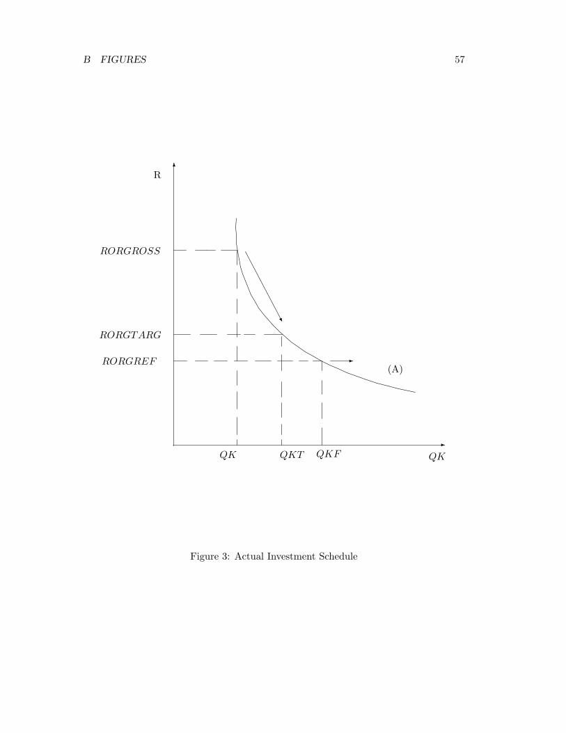
of return schedule, relating the expected rate of return to the size of the capital stock:

RORGEXP(r)

RORGREF (r)=

[

QK (r)

QKF (r)

]−RORGFLEX (r)

, (43)

where RORGEXP(r) denotes the expected gross rate of return and RORGFLEX (r) a RORGEXPRORGFLEX

positive parameter, representing the absolute magnitude of the elasticity of the expected

rate of return with respect to the size of the capital stock. RORGREF (r) denotes a RORGREF

reference rate of return in region r, and QKF (r) a reference capital stock. Investors QKF

expect that if the actual capital stock QK is equal to the reference stock QKF , then

the rate of return will be equal to the reference rate RORGREF . If the capital stock


exceeds the reference stock, the expected rate of return is less than the reference rate;

if the capital stock is less than the reference stock, the expected rate is greater than

the reference rate.

In dealing with expectations, as in equation (43), there are two relevant times: the

time at which the expectations are held, and the time to which they refer. We call

these respectively the expectation time and the realization time. So for example, in

describing an investor in 2000 holding an expectation about the rate of return in 2005,

the expectation time is 2000 and the realization time 2005.

In the theory underlying the investment module, expectation time is always just the

current time TIME for the model. For example, if the model represents the state of

the world economy in the year 2000, then expectations time is 2000. Realization time

TREAL however may be either the current or some future time. In the model itself,

as opposed to the underlying theory, expectation time and realization time are always

equal to the current time; so in the model equations TREAL would be redundant, and

we use only the current time TIME .

To complete our description of investor expectations in equation (43), we need

to specify how the reference rate of return and the reference capital stock depend

on realization time. We postulate that the reference rate of return is independent of

realization time, while the reference capital stock grows at some normal rate KHAT (r): KHAT

QKF (r) = QKO(r)eKHAT (r)TREAL, (44)

where QKO(r) denotes the reference capital stock at some base time TREAL = 0. QKO

Under this treatment, the normal rate of growth KHAT (r) is the rate at which the

capital stock can grow without (as investors expect) affecting the rate of return. If the

capital stock grows at a rate greater than KHAT (r), investors expect rates of return to

decline through time; if the capital stock grows at less than KHAT (r), investors expect

rates of return to fall.

The specification of expectations in equations (43) and (44), while simple, is intended

to approximate the actual investment schedule. In particular, it allows a range between

zero and infinity to the gross rate of return RORGROSS (r). This allows, realistically,

that the net rate of return may sometimes be negative. Whether the specification is

locally model-consistent depends on the setting of the normal growth rate KHAT (r)

and the elasticity RORGFLEX (r). As discussed in subsection 5.4, we allow model-

consistent adjustment of KHAT (r). RORGFLEX (r), however, is fixed; we can set

it initially at a locally model-consistent value, but through a simulation or series of

projections, it typically becomes more or less inconsistent. This is undesirable, but also


unavoidable without a considerable increase in the complexity of the theory.

To find the expected rate of growth in the rate of return, we differentiate equa-

tion (43) with respect to realization time, substituting for QKF (r) from equation (44),

obtaining

ERG RORG(r) = −RORGFLEX (r)(RG QK (r)−KHAT (r)), (45)

where ERG RORG(r) denotes the expected rate of growth in the rate of return in ERG RORG

region r, and RG QK (r) the rate of growth in the capital stock. Now the rate of RG QK

growth in the capital stock,

RG QK (r) =dQK (r)/dTIME

QK (r)

=QCGDS (r)− RDEP(r)QK (r)

QK (r)

=QCGDS (r)

QK (r)− RDEP(r),

where QCGDS (r) denotes the level of investment in region r. Substituting into equa- QCGDS

tion (45), we obtain

ERG RORG(r) = −RORGFLEX (r)

(

QCGDS (r)

QK (r)− RDEP(r)−KHAT (r)

)

. (46)

Totally differentiating, we obtain

erg rorg(r) = −RORGFLEX (r)[IKRATIO(r)(qcgds(r)− qk(r))−DKHAT (r)], (47)

where erg rorg(r) denotes absolute change in the expected rate of growth in the rate of erg rorg

return in region r, IKRATIO(r), the ratio QCGDS (r)/QK (r) of gross investment to IKRATIO

the capital stock, qcgds(r), percentage change in investment, and DKHAT (r), absolute qcgdsDKHAT

change in the normal rate of growth in the capital stock. Then, in the model we have:

Equation E_erg_rorg

#behavioral equation for expected rate of growth in rate of return#

(all,r,REG)

erg_rorg(r)

= -RORGFLEX(r)*[IKRATIO(r)*[qcgds(r) - qk(r)] - DKHAT(r)];

As equation (47) shows, the expected rate of growth in the rate of return varies

inversely with the level of investment. Then the level of investment is given implicitly


by the condition that the expected rate of growth be equal to the required rate,

ERG RORG(r) = RRG RORG(r). (48)

We depict some aspects of the investment theory in figure 3. Each point in the figure

represents a (capital stock, rate of return) pair (QK , R). The curve (A) represents

the expected rate of return schedule for realization time equal to expectation time;

it is downward sloping, with slope related to the elasticity RORGFLEX , a vertical

asymptote at QK = 0, and a horizontal asymptote at R = 0. It passes through the

point (QK ,RORGROSS ) representing the current capital stock and rate of return,

and also through the reference point (QKF ,RORGREF ); the reference point adjusts

implicitly to allow this.

For a realization time greater than the expectation time, the curve would be similar

to (a) but dilated about the vertical axis; assuming a positive normal growth rate, the

curve would dilate rightward as realization time increased.

As we have drawn the figure, the actual rate of return RORGROSS exceeds the

target rate RORGTARG . From equation (39), this implies that the required rate of

growth in the rate of return is negative; on the diagram, this implies some required

downward vertical speed. Inverting equation (46) and equating the required rate of

return to the expected rate, we find the required level of investment,

QCGDS (r) = QK (r)[RDEP(r) +KHAT (r)− RORGFLEX (r).ERG RORG(r)].

Here QK (r).RDEP(r) is the investment level required to maintain the capital stock

QK (r) at its current level, QK (r).KHAT (r) the further investment required to

keep pace with the rightward dilation of the rate of return curve (A), and QK (r)

.RORGFLEX (r).ERG RORG(r) the further investment required to maintain the re-

quired vertical speed down the curve.

5.3 Adaptive expectations

In practice, the investment theory as presented to this point in equations (40),

(47), and (48) has a significant disadvantage. Using information in the benchmark

data, we can calculate the actual rate of return RORGROSS (r) in the initial year. The

rate of return and the equations of the model allow us to determine the level of invest-

ment QCGDS (r). However, the benchmark data also specifies the level of investment.

This level, in general, will be inconsistent with the level calculated with the theory.

Consider, for example, the region with the highest rate of return in the data base.


In this region the actual rate of return exceeds the target rate, so the required rate of

growth in the rate of return RRG RORG(r) is negative. This, in turn, implies that

the normal rate of growth in the capital stock KHAT (r), and investment QCGDS (r)

should be high. However, it may be that the level of investment recorded in the data

base is not particularly high. In this case, theory and data are inconsistent. We could

modify the data by lowering the rate of return, or we could generalize the theory to

achieve such an outcome.

We can resolve this inconsistency by modifying either the data or the theory. One

approach to modifying the data involves equalizing rates of return across countries in

the data base. This conflicts with one of our objectives for the dynamic model, that

it should work with data bases that conform closely to observed statistics, rather than

requiring a heavily recalibrated or stylized data base. Another approach would be to

account for investment level anomalies through risk premia; we can do this readily in

the data base, without touching the flows data, by adjusting the target rates. This

option is sometimes appealing; we do not wish however to force it on users. Rather we

recognize that reality is under no obligation to respect our (or any other) investment

theory, and that for a multitude of reasons, observed investment levels will surely differ

from any theoretical prediction. We therefore extend the theory so that it does not

prescribe investment levels, but accommodates the observed investment levels over the

short run, while still maintaining the old theory’s long-run properties.

We achieve the desired relaxation by letting investors react to expected rather than

actual rates of return. With this approach we can account for any observed level of

investment, by setting the expected rate of return so as to warrant that investment level.

At the same time, by incorporating an adjustment mechanism that draws the expected

rate of return gradually toward the actual rate, we retain the long-run properties of the

simpler theory, including long-run equalization of rates of return. Furthermore, this

way of accounting for observed investment levels has some theoretical appeal.

Investment is undertaken with the expectation of deriving returns over some period

of time. Thus, investors are concerned not only with the rate of return at the moment

of purchasing an asset, but also with the rate of return throughout its life. Investors’

expectations are also “sticky” or “sluggish”. When the observed rate of return changes,

investors are unsure whether this change is transient or permanent. They adjust their

expectations of future rates of return only with a lag. At first investors make a small

adjustment, then if the change in the actual rate persists, they make further changes

in expectations, until eventually the expected rate conforms to the observed rate.

Earlier (subsection 5.1), we represented investors’ reactions to current returns


through equation (40):

rrg rorg(r) = LAMBRORG(r) ∗ [rorgt(r)− rorga(r)].

To let investors react to the expected rate of return rather than the actual rate, we

replace the actual rate of return variable rorga with the expected rate variable rorge. rorge

At the same time, we enforce the condition that the expected rate of growth in the rate

of return be equal to the required rate, by replacing the required rate rrg rorg with the

expected rate erg rorg . This gives us the final form of the equation,

erg rorg(r) = LAMBRORG(r) ∗ [rorgt(r)− rorge(r)], (49)

In the model, we implement this as:

Equation E_erg_rorg # rule for investment # (all,r,REG)

erg_rorg(r) = LAMBRORG(r)*[rorgt(r) - rorge(r)];

We now need to specify an error correction mechanism bringing the expected rate

rorge closer through time to the actual rate rorga. We recall equation (43) for the

expected rate of return schedule,

RORGEXP(r)

RORGREF (r)=

[

QK (r)

QKF (r)

]−RORGFLEX (r)

,

and note a few points:

• Even before the theoretical extension introduced in this subsection, we already

have a concept of an expected rate of return.

• Previously, however, the expected rate of return schedule was such that, at the

current capital stock and the current time, the expected rate of return was equal

to the actual current rate of return. Now we allow that the expected current rate

of return may differ from the actual rate.

• As specified by the expected rate of return schedule, the expected rate of return

is conditional on the capital stock, and also on realization time. This rules out a

simple adjustment rule for the expected rate of return, such as

rorge(r) = 100.LAMBRORGE (r)

[

logrorga(r)

rorge(r)

]

time.

This would represent investors as perversely ignoring the effects of investment and

economic growth on the rate of return. Rather than an adjustment rule for the


rate of return itself, we need an adjustment rule for the rate of return schedule,

shifting so that through time the expected current rate of return draws closer to

the actual current rate.

• From equations (43) and (44), we note that the position of the rate of return

schedule is given by the reference rate of return, RORGREF (r), and the base

time value of the reference capital stock, QKO(r).

To specify an error correction mechanism for the rate of return schedule, we define

the warranted reference rate of return, RORGFWARR(r), as value for the reference

rate that equates the expected rate RORGEXP(r) to the actual rate RORGROSS (r)

in equation (43). Then the warranted reference rate of return is given implicitly by the

equation

RORGROSS (r)

RORGFWARR(r)=

[

QK (r)

QKF (r)

]−RORGFLEX (r)

. (50)

From equations (43) and (50), we have

RORGFWARR(r)

RORGREF (r)=

RORGROSS (r)

RORGEXP(r). (51)

We postulate an error correction process, through which the reference rate of return

draws closer through time to the warranted rate:

rorgf (r) = 100.LAMBRORGE (r)

[

logRORGFWARR(r)

RORGREF (r)

]

time,

where rorgf (r) denotes percentage change in the reference rate of return, and

LAMBRORGE (r) an adjustment coefficient. Substituting from equation (51), we obtain LAMBRORGE

rorgf (r) = −100.LAMBRORGE (r)

[

logRORGEXP(r)

RORGROSS (r)

]

time

= −100.LAMBRORGE (r).ERRRORG(r).time, (52)

where ERRRORG(r) is a measure of error in the expected rate of return, ERRRORG(r) = ERRRORG

log(RORGEXP(r)/RORGROSS (r)).

Having specified this error correction mechanism for the expected rate of return

schedule, we can now derive the error-correcting equation for the expected rate of

return itself. Recalling equation (44)

QKF (r) = QKO(r)eKHAT (r)TIME ,


we substitute into equation (43), obtaining

RORGEXP(r)

RORGREF (r)=

[

QK (r)

QKO(r)eKHAT (r)TIME

]−RORGFLEX (r)

.

At this point, we add one final feature. For various reasons, users may sometimes

wish to intervene in the expectations-setting process. They may wish to add some addi-

tional shock to the expected rate of return, or they wish to deactivate the expectations

rule, so as for example to set the investment level directly. To allow this, we add a

shift factor SRORGEXP(r) to the expected rate equation. This normally is exogenous SRORGEXP

and zero; it may be given a non-zero value to add exogenous shocks to the expectation-

setting process, or endogenized to disable the expectations rule so that, for example,

the investment level may be set directly. This gives us the final form for the levels

equation,

RORGEXP(r)

RORGREF (r)= SRORGEXP(r)

[

QK (r)

QKO(r)eKHAT (r)TIME

]−RORGFLEX (r)

.


rorge(r) = rorgf (r)− RORGFLEX (r)(qk(r)− 100.KHAT (r).time) + srorge(r),

where srorge(r) denotes percentage change in the expected rate shift factor. Substitut- srorge

ing for rorgf from equation (52), we obtain

rorge(r) = −RORGFLEX (r)(qk(r)− 100.KHAT (r).time)

−100.LAMBRORGE (r).ERRRORG(r).time

+srorge(r). (53)

This equation shows three sources of change in the expected rate of return: divergence

between the actual rate of growth in the capital stock, qk(r)/[100.time], and the normal

growth rate KHAT (r); a correction for the observed error in the expected rate; and an

exogenous shift factor. We implement this in the model as

Equation E_rorge #rule for expected gross rate of return# (all,r,REG)

rorge(r)

= -RORGFLEX(r)*[qk(r) - 100.0*KHAT(r)*time]

- 100.0*LAMBRORGE(r)*ERRRORG(r)*time

+ srorge(r);


5.4 The normal rate of growth in the capital stock

As noted in subsection 5.2, whether the expected growth rate ERG RORG is model-

consistent depends in part on the normal growth rate KHAT . In some early versions

of the model, we treated KHAT as a fixed parameter, and calibrated it before each

base case projection (that is, the series of projections forming the base case for some

collection of experiments with the model), to ensure that it was consistent with the long-

run behavior of the model. This had two disadvantages. It forced us to calibrate the

parameter anew for each base-case projection, and this was somewhat onerous. Also,

it held KHAT constant within each projection, and this was not always appropriate.

For example, it would not be appropriate to a projection involving slow technological

progress through the 1980s, but faster progress through the 1990s. We could avoid this

by setting several different KHAT values for different periods within the projection,

but that involved yet more calibration simulations.

To avoid these problems, we now treat the normal growth rate KHAT as an up-

dateable coefficient within the model, and provide an adjustment mechanism to bring

it towards a model-consistent value through the course of a simulation. We postulate

an adjustment mechanism

DKHAT (r) = 100.LAMBKHAT (r)(KHAPP(r)−KHAT (r))time, (54)

where LAMBKHAT (r) denotes a coefficient of adjustment, and KHAPP(r) the appar- LAMBKHAT

ent current normal growth rate in region r.

By the apparent current normal growth rate, we mean the normal growth rate

implied by current changes in the capital stock and the rate of return, and by the

assumed elasticity RORGFLEX . If the rate of return is currently constant, then it

appears that the capital stock is growing at the normal rate, so the apparent normal

rate is equal to the actual rate. If the rate of return is rising, then the apparent normal

rate is greater than the actual rate; if the rate of return is falling, the apparent normal

rate is lower than the actual rate.

To calculate the apparent normal rate, we return to the expected investment sched-

ule equation (43), assume that it agrees with the actual schedule, and solve for the

apparent value KHAPP of the normal growth rate KHAT . We thus obtain

KHAPP(r) = RORGFLEX (r)−1ARG RORG(r) +QCGDS (r)

QK (r)− RDEP(r).

This shows that the apparent normal growth rate KHAPP(r) is equal to the actual

growth rate QCGDS (r)/QK (r) − RDEP(r), plus an adjustment RORGFLEX (r)−1


ARG RORG(r) for current growth in the rate of return. Substituting into equa-

tion (54), we obtain

DKHAT (r) =

100.LAMBKHAT (r)(

RORGFLEX (r)−1ARG RORG(r) +QCGDS (r)

QK (r)− RDEP(r)−KHAT (r)

)

time. (55)

Now adapting equation (7), we have

100

(

QCGDS (r)

QK (r)− RDEP(r)

)

time = qk(r).

Also, by definition of ARG RORG(r) we have

100.ARG RORG(r) time = rorga(r).

Substituting into equation (55), we obtain

DKHAT (r) = LAMBKHAT (r)(

RORGFLEX (r)−1rorga(r) + qk(r)− 100.KHAT (r).time)

. (56)

Translating into TABLO code, we have in the model

Equation E_DKHAT

#behavioral equation for estimated normal rate growth rate#

(all,r,REG)

DKHAT(r)

= LAMBKHAT(r)

* [qk(r) + [1.0/RORGFLEX(r)]*rorga(r) - 100.0*KHAT(r)*time];

Figure 4 shows two rate-of-return curves: the expected rate curve (E), passing

through the current capital stock and expected current rate of return, (QK ,RORGEXP);

and the warranted curve (A), passing through the current capital stock and actual cur-

rent rate of return, (QK ,RORGROSS ). As before, the expected investment curve

dilates rightward through time at a rate given by the normal rate of growth in the

capital stock KHAT (or leftward, if KHAT is negative). But now it also dilates ver-

tically, so as to draw closer to the warranted curve (A). Now the shape of the curve

is such that any vertical dilation is equivalent to a horizontal dilation, and vice-versa;


specifically, a vertical dilation by a factor V is equivalent to a horizontal dilation by a

factor V RORGFLEX . So we may say simply that the curve dilates inward or outward, at

a rate depending on the normal growth rate KHAT , but adjusted so as to draw closer

to the warranted curve (A).

As the expected rate curve dilates outward, so too does the warranted rate curve,

at a rate described by the apparent normal growth rate KHAPP .

If the error in expectations is zero (RORGEXP(r) = RORGROSS (r)) and the

expected normal growth rate KHAT agrees with the apparent rate KHAPP , then the

expected rate and warranted rate curves (E) and (A) coincide, and furthermore, dilate

outward together at the same rate so as to remain coincident.

If the error in expectations is zero (RORGEXP(r) = RORGROSS (r)), but the ap-

parent normal growth rate KHAPP exceeds the expected normal growth rate KHAT ,

then the expected rate curve (E) and the warranted rate curve (A) are initially coinci-

dent, but the warranted rate curve dilates outward faster than the expected rate curve.

Through the normal rate adjustment process, the normal rate accelerates toward the

apparent rate, pushing the velocity of the expected rate curve closer to that of the

warranted rate curve; while the rate of return adjustment process pushes the position

of the expected rate curve closer to that of the warranted rate curve.

If the expected normal growth rate KHAT agrees with the apparent growth

rate KHAPP , but the expected rate of return RORGEXP exceeds the actual rate

RORGROSS , then the expected rate curve (E) lies outside the warranted rate curve

(A). Then the expected rate curve dilates outward at less than the normal rate, allowing

the warranted rate curve to catch up with it.

5.5 Summary

Equations (49), (47), (56), and (53), shown in Table 1, comprise the investment theory

of adaptive expectations and jointly determine the forward-sloping regional supply of

investment funds. With this set of equations, there is perfect capital mobility only over

the long run as regional rates of return gradually adjust towards a common target rate.

Equation (53) both determines the expected rate rorge and (in figure 4) governs

the position of the expected rate curve (E). It lets the expected rate curve (E) dilate

outward at a rate governed partly by equation (56) and partly by a catch-up component

drawing toward the warranted rate curve (A). Equation (56) coordinates the movements

of curves (A) and (E) so that (abstracting from the catch-up effect) their velocities draw

together. Equation (49) specifies the required rate of growth in the expected rate of

return— the required vertical velocity of the point (QK ,RORGEXP) in figure 4; and


equation (47) translates this into a required level of investment, or horizontal velocity

within the figure, given the vertical velocity and the requirement that the point lie

on the expected rate curve (E). Thus, equations (49), (47), (56), and (53) determine

regional investment, and, via the accumulation equation (10), regional capital stocks in

GTAP-Dyn.

To illustrate the disequilibrium nature of the adjustment mechanism in this model,

let us assume initially an equality between the actual, expected, and target rates of re-

turn. This equality implies that the actual and expected schedules overlap and move to-

gether in response to changes in the normal rate of growth in the capital stock KHAT (r).

If there is a positive shock to productivity, the actual rate of return increases and the

warranted rate schedule (A) moves to the right of the expected rate schedule (E). The

model detects the acceleration in economic growth via equation (56) in the initial period

of the shock, which leads to an increase in regional investment via equation (47). Next

period, a further increase in the expected normal growth rate KHAT (r) leads to a fur-

ther rise in regional investment. Graphically, this is represented by an outward dilation

of the expected rate curve. In addition, via the second term of equation (53), investors

realize that the expected rate of return is lower than the actual rate of return. This

leads both to a further outward dilation of the expected rate curve toward the warranted

rate curve, and, through equation (49), a decrease in the required rate of growth in the

rate of return, RRG RORG . Equation (47) translates this into a rightward movement

qcgds along the expected rate curve.

Taking these four equations together, together with the equations (41) and (42)

for rorgt , we may regard them as an equation subsystem. With a normal closure, the

subsystem takes as given the variables qk , SDRORT , srorge, and time, and one degree

of freedom of qcgds (qcgds is constrained by the requirement that the money value

of world investment must equal world saving). It determines the variables qcgds and

SDRORTW . The variables DKHAT , DRORT , erg rorg , rorge, and rorgt are internal

to the subsystem.

In its relations with the rest of the equation system, this subsystem has some notable

features. It may be surprising that the capital stock qk(r) helps to determine the

investment level. Referring back to the derivation of equation (47), we see that achieving

a given expected rate of growth in the rate of return entails achieving a certain rate

of growth in the capital stock; the level of investment required to achieve that rate of

growth depends on the size of the capital stock. The capital stock thus serves as a

scaling factor for investment.

Equally notable is the absence of certain links from the equation system. We ex-

pect the actual rate of return to affect the expected rate, yet in the expected rate of


return equation (53) the variable rorga(r) does not affect rorge(r). Equally, we expect

investment to affect the capital stock, yet in the capital accumulation equation (10),

the variable qcgds(r) does not affect qk(r). The explanation is that these links do exist

in the theoretical structure, but through coefficients rather than variables. The level

of the actual rate of return affects the coefficient ERRRORG(r), which appears in the

expected rate of return equation and affects the variable rorge(r). Similarly, the level

of gross investment affects the coefficient NETINV (r), which appears in the capital

accumulation equation and affects the variable qk(r).

5.6 Alternative investment determination

In some simulations, the user may wish to disable the investment theory described in

the preceding subsections and instead impose specific investment targets. For example,

she may wish to use investment forecasts from macroeconomic models, or to model

sudden (perhaps dramatic) fluctuations in investment, such as those observed in the

Asian crisis.

Imposing investment targets on all regions is harder than it may at first seem.

Through the identity that world saving is equal to world investment, it would implicitly

impose a target on world saving. To accommodate that, the user would need to change

the treatment of saving in the closure. In this section we consider a more limited

objective, imposing targets on regional shares in world investment, while allowing the

usual saving theory to determine its level.

To enable this, we use an equation

QCGDS (r) = SQCGDSREG(r).SQCGDSWORLD ,

representing investment in region r as the product of a region-specific factor

SQCGDSREG(r) and a region-generic factor SQCGDSWORLD. Differentiating, we SQCGDSREGSQCGDSWORLD

obtain

qcgds(r) = sqcgdsreg(r) + sqcgdsworld , (57)

where sqcgdsreg(r) and sqcgdsworld denote percentage changes in SQCGDSREG(r) sqcgdsregsqcgdsworld

and SQCGDSWORLD . In the TABLO code, we write

Equation GDI # region specific determination of investment #

(all,r,REG)

qcgds(r) = sqcgdsreg(r) + sqcgdsworld;

Normally sqcgdsworld is exogenous and sqcgdsreg(r) endogenous, so that the GTAP-

Dyn investment theory determines qcgds(r) and equation (57) determines sqcgdsreg(r).

6 PROPERTIES AND PROBLEMS 44

But when we wish to target the regional allocation of investment, we exogenize sqcgdsreg

and endogenize either srorge or SDRORT . At the same time, we exogenize SDRORTW

and endogenize sqcgdsworld , letting sqcgdsworld adjust so that global investment re-

mains equal to global saving.

If we wish to target the investment allocation in all periods, it does not matter

whether we endogenize srorge or SDRORT . If however we wish to target it only in

earlier periods, but let the investment theory drive it in later periods, then the choice

of variable does matter.

If in the earlier periods we endogenize srorge, the model achieves the investment tar-

gets by adjusting expected rates of return. In the later periods, with srorge exogenous,

the expected rates converge toward the actual rates according to the usual GTAP-Dyn

theory. So under this treatment, the imposed investment allocation is transient.

If however in the earlier periods we endogenize SDRORT , the model achieves

the investment targets by adjusting target rates of return. In the later periods, with

SDRORT exogenous, the differentials in the target rates remain in place, unless and

until we shock them back toward equality. So under this treatment, the imposed in-

vestment allocation is persistent.

6 Properties and problems

Having completed the presentation of the GTAP-Dyn theoretical structure, we now

discuss some properties of the system, and issues arising in using it.

• existence and stability of long-run equilibrium,

• cumulative and comparative dynamic results,

• path dependence,

• one-way relations,

• capital account volatility and the propensity to save.

6.1 Long-run equilibrium

In the GTAP-Dyn investment theory (section 5), expected, target, and actual rates of

return may all differ over the short run. In long-run equilibrium, these three rates are

all equal, and constant over time, as is also the normal growth rate for the capital stock:

RORGEXP(r) = RORGTARG(r) = RORGROSS (r), ∀r (58)


˙RORGEXP(r) = ˙RORGTARG(r) = ˙RORGROSS (r) = 0, ∀r (59)

KHAT (r) = 0, DKHAT (r) = 0, ∀r. (60)

These conditions imply in turn a constant investment-capital ratio. They are the same

conditions characterizing the equilibrium solution of a multi-region q-investment model

with convex adjustment costs.

Ianchovichina (1998) demonstrates the existence and stability of the long-run equi-

librium. Here we provide a numerical illustration. We use a three-region aggrega-

tion of the version 3 GTAP data base (McDougall 1997) featuring the United States

(USA), the European Union (E U), and all other regions aggregated into a rest-of-

world region (ROW). The initial data (1992) reveal regional differences in rates of

return, RORGROSS (r) (Figure 5), normal rates of growth in capital KHAT (r) (Fig-

ure 7), investment-capital ratios (Figure 8), as well as sizable errors in expectations

ERRRORG(r) (Figure 6). In short, the benchmark data depict a world in disequilib-

rium.

We test the long run properties of the model over a hundred year period. The

simulation represents the changes in the three economies occurring solely due to the

passage of time. It depicts the movement from the initial disequilibrium state towards

a long-run equilibrium. For simplicity, we assume zero regional risk premia.

Figure 6 suggests that in 1992 investors underestimated returns to capital in the

United States and the rest of the world and overestimated returns to capital in the

European Union. As investors realize their errors in predicting these returns, they ad-

just their expectations in an upward direction in the case of the United States and the

rest-of-world region, and in a downward direction in the case of the European Union

(via equation (53)). As a result, investment in the United States and the rest of the

world increases, while investment in the European Union declines (via equations (49)

and (47)). It takes approximately 12 years for the model to eliminate errors in expec-

tations (Figure 6) and inter-regional differences in rates of return (equilibrium condi-

tion (58), Figure 5). However, since KHAT (r) is neither zero nor a constant in 2004,

this is only a temporary equilibrium. Positive and nonconstant KHAT (r) (Figure 7)

implies that the expected investment schedule (43) will overshoot the warranted one

(50), and over time will start moving back. We observe this type of oscillating behavior

on Figures 5, 6, 7, and 8 around 2004. Only after further reduction in KHAT via equa-

tion (56), leading to a reduction in the investment-capital ratio via equation (47), will

the model permanently eliminate errors in expectations and differences in inter-regional

rates of return.

Figure 5 shows the convergence of the regional rates of return RORGROSS (r) to-


wards the target rate RORGTARG(r), and Figure 6 shows the elimination of errors in

expectations ERRRORG(r) over time. Figure 7 displays the normal rate of growth in

the capital stock KHAT (r) in its movement towards 0 over the long-run, while Figure 8

demonstrates the process of adjustment towards constant investment-capital ratios.

The three figures suggest that the stability conditions of the model are satisfied over

time.

6.2 Cumulative and comparative dynamic results

GTAP-Dyn is designed as a recursive dynamic model. To obtain projections through

time, you run a sequence of simulations, one for each time period in the projection. To

obtain comparative dynamic results, you run two sequences of simulations, one repre-

senting a base case projection and the other representing a variant projection. From the

period-by-period results, you then calculate cumulative results for each projection. Fi-

nally you difference the two series of cumulative results to obtain comparative dynamic

results.

The formulas used for cumulating and differencing are different for the different

kinds of variable distinguished in GEMPACK, change and percentage change. For a

change variable dV , the cumulative change over two periods 1 and 2,

dV02 = dV01 + dV12,

where the subscript 01 denotes changes between the start and end of period 1, and 12,

changes between the end of period 1 and the end of period 2. For a percentage change

variable v, we have a more complex formula,

v02 = 100

[(

1 +v01

100

)(

1 +v12

100

)

− 1

]

.

This procedure works for most of the variables in the model, but not for all. In

particular, it does not work for the equivalent variation, EV (r), and associated vari-

ables. The problem is that the variable is defined so that, in say the first period, the

equivalent variation variable is

EV01 = E(U1,P0)− E(U0,P0),

where E is the expenditure function, U , utility, P, prices, and the subscripts 0 and 1

refer to values at the beginning and end of the first period. In the second period, we


have

EV12 = E(U2,P1)− E(U1,P1).

Then the cumulative equivalent variation for the first and second periods,

EV02 = E(U2,P0)− E(U0,P0);

but we cannot calculate this from EV01 and EV12. Thus we cannot calculate valid

cumulative results for the equivalent variation; nor, consequently, valid comparative

dynamic results. Similarly, we cannot calculate valid comparative dynamic results for

the equivalent variation decomposition (Huff and Hertel, 1996).

This does not mean that we cannot obtain comparative dynamic results for equiva-

lent variation; to obtain them however, we need some computational machinery beyond

the cumulating and differencing procedures used for other variables.

6.3 Path dependence

GTAP-Dyn is inherently a path-dependent model. That is, in GTAP-Dyn, the effects

of changes in exogenous variables depend not only on the overall changes in but also

on the paths followed by, the exogenous variables. When GTAP-Dyn is used as a

dynamic model— when the time variable time is shocked— this means that the effects

of economic shocks depend not only on the size but also on the timing of the shocks.

Path dependence is built into the theory in three places: wealth accumulation (sub-

section 4.3), the partial adjustment treatment of the capital stock (subsection 5.1),

and the adaptive expectations treatment of the expected rate of return and the normal

growth rate (subsections 5.3 and 5.4).

In the GTAP-Dyn theory, a region’s wealth depends on its past history; it cannot

be determined from other current variables, such as income. The final level of regional

wealth in any simulation depends on the original level, and on the time paths of the

exogenous variables within the simulation. For example, technological progress in a

given region normally leads to an increase in its wealth; but the increase in wealth is

greater if the technological progress occurs mostly near the beginning of the period than

if it occurs mostly toward the end. Other path dependencies arise from the lagged ad-

justment treatment of the capital stock, and from the adaptive expectations treatment

of investment.

Similarly, regional capital stocks cannot be inferred from other current variables.

There are two reasons for this. Globally, the money value of net physical investment is

equal to saving, so the money value of the global capital stock is determined by wealth


accumulation (and capital gain), not by an equilibrium condition. Also, the distribution

of capital across regions is given not by an equilibrium condition but by a partial

adjustment process, as described in subsection 5.1. Investors do redistribute capital

to equalize rates of return, but only gradually; past shocks therefore have affected the

current international distribution of capital more if they occurred in the more distant

past, less if they occurred in the more recent past.

Finally, the level of investment depends not on the actual rate of return but on the

expected rate. And the expected rate of return cannot be inferred from other current

variables, but adjusts toward the actual rate with a lag (as described in subsection 5.3).

Here then is yet another adjustment process whose results depend not only on the size

of the changes in its inputs, but also on their timing.

Given GTAP-Dyn’s objectives, this path dependence must be construed not as a

bug but a feature. Indeed, if we should extend GTAP-Dyn to provide a better treatment

of short-run dynamics, bringing in more macroeconomic content such as that found in

such models as G-CUBED or FAIR, path dependencies will become more pervasive rather

than less. In short, path dependence in GTAP-Dyn is here to stay.

Nevertheless (and this is why one might be tempted to construe it as a bug) path

dependence imposes some practical inconveniences. It places on the user an onus to

represent accurately the time paths of exogenous variables, in circumstances where it

would otherwise be unnecessary. Users need to take it into account in several places in

their computational strategy.

First, you need to set periods, within the overall projection time interval, to capture

sufficient detail about the time profile of the shocks. With the continuous time approach

used in GTAP-Dyn, you can run say a tariff reduction scenario over a single ten-year

interval and get sensible and meaningful results. If however you want the tariff cuts

to be not implemented at an even pace but backloaded, then you need to use several

shorter intervals, so that you may specify lower rates of tariff reduction in the earlier

intervals, and higher rates in the later intervals.

Second, even if you wish to apply shocks evenly through time, you may wish to

avoid long time intervals, if you do not like the rule TABLO uses to distribute shocks

between steps. TABLO-generated programs distribute shocks so that the change in the

levels variable is the same for all steps (Harrison and Pearson 1998, ch. 4, “GEMSIM

and TABLO-generated Programs”). So (to take an extreme example) if you shock a

variable by 300%, using a two-step solution procedure, your TABLO-generated program

shocks the variable by an amount equivalent to 150% of the initial level in each step;

that is, by 150% in the first step (going from 1 to 2.5 times the initial level), and 60%

in the second step (going from 2.5 to 4 times the initial level).


For most percentage change variables, in most applications, a more appealing default

assumption is that the percentage change in the variable is constant across steps. For

example, it is more natural to assume that the population grows at a constant rate

through time (for example, by 1 per cent per year) than that it changes at a constant

rate (for example, by 200,000 persons per year). Likewise, in the extreme example given

previously, we would typically prefer by default to shock the variable by 100% in each

step, rather than by 150% in the first step and 60% in the second. GEMPACK wizards

may perhaps know some way to coerce TABLO to use equal percentage changes; none

however is apparent from the published documentation.

The shock-splitting rule does not much matter when the shocks are small, but it

does matter when they are large. More specifically, it matters when the total shock

in a simulation is large, even if the shock is broken up into small pieces in individual

steps. One way to work around the problem is to avoid long intervals always, even if

all shocks are evenly distributed through time.

Finally, path dependence rules out some common closure-swapping strategies. In

GEMPACK, a common expedient is to let the model determine the change in some in-

strument variable required to achieve a given change in a target variable, by making the

(naturally exogenous) instrument variable endogenous, and the (naturally endogenous)

target variable exogenous. For example, we may determine the rate of technological

progress required to achieve a given improvement in welfare, by endogenizing the tech-

nological change variable and exogenizing the welfare variable. If we then run a second

simulation, using the natural closure, and shocking the technological change variable

according to the results from the first simulation, we get—with a path-independent

model— the same results as in the first simulation. We can then investigate the effects

of changes in other elements of the scenario, on welfare as on other variables, using the

natural closure and the calibrated technological change shock.

With a path-dependent variable this does not work. The trouble is that the path

of the technological change variable is different in the two simulations. In the second

simulation, technology changes evenly through the simulation interval; in the first, it

changes so as to keep GDP moving evenly through the interval. This is liable to affect

the simulation results. In GTAP-Dyn, for example, a front-loaded improvement in

technology has more effect on end-of-interval wealth than the same total improvement

distributed evenly through the interval.

What we need (but, at the time of writing, do not have) for this problem is an

automated algorithm for finding the constant rate of growth in an instrument variable

(or the constant rates of growth in a set of instrument variables) that achieves given total

growth in a target variable (or a set of target variables). Such a tool would be useful


not only for single-simulation but also for multi-simulation projections. For example,

in a projection made up of five two-year simulations, each involving say different tariff

shocks, we would like to be able to find the constant rate of technological progress,

through the complete ten-year projection interval, required to achieve a given welfare

improvement over the interval. Such a multi-simulation facility would be useful even

with path-independent models.

6.4 One-way relations

A novel emergent feature of GTAP-Dyn, relative to standard GTAP, is the appearance

of what we here describe as one-way relations.

In standard GTAP, as perhaps in most GEMPACK-implemented models, if an ex-

ogenous variable A affects an endogenous variable X, we can swap A and X in the

closure, and determine in a simulation the change in A required to bring about a given

change in X. Of course, this may not work if X is not monotonic in A, but it works

most of the time (and, of course, it always works for sufficiently small changes in X if X

is locally non-stationary in A). In GTAP-Dyn however it may easily fail. That is, there

are relations between variables A and X such that the solution program can determine

the change in X arising from a given change in A, but not the change in A required

to bring about a given change in X— no matter how well-behaved mathematically the

relation between A and X.

These one-way relations appear when one variable affects another not through the

equation system but through data updates. For example, investment of course affects

the capital stock; yet the investment variable (qcgds) does not appear in the relevant

equation (equation 10),

VK (r) . qk(r) = VK (r)[sqkworld + sqk(r)] + 100NETINV (r) . time.

Instead, the equation contains the investment coefficient NETINV . In a single-step

simulation, qcgds has no effect on qk ; in a multi-step simulation, it affects NETINV

at each update of the data files, and thereby affects qk .

Now consider the effect of a shock to a normally exogenous, investment-related

variable, for example, the target rate shift variable SDRORT . In each period, this

leads through the investment module, to some change in the investment variable qcgds,

But that change in qcgds has no effect in the current period on qk .

If we try to change the closure to find the SDRORT value consistent with a given

change in qk , we find it impossible. If we exogenize qk(r) (for some region r) and

endogenize SDRORT (r), we make the model singular, since we thereby make exogenous


all variables in equation (10). The only natural way to exogenize qk(r) is to swap it

with sqk(r), and that does not achieve the larger purpose, since it does not allow qk(r)

to determine qcgds(r) or SDRORT (r).

Another one-way relation is that between the actual rate of return RORGROSS

and the expected rate RORGEXP . According to the GTAP-Dyn theory, changes in

RORGEXP cause changes in RORGROSS , yet rorga does not appear in the equation

for rorge, equation (53),

rorge(r) = −RORGFLEX (r)(qk(r)− 100.KHAT (r).time)

−100.LAMBRORGE (r).ERRRORG(r).time

+srorge(r).

In a single-step simulation, indeed, rorga has no effect on rorge; in a multi-step sim-

ulation however, it affects ERRRORG at each data file update, and thereby affects

rorge.

If you shock some exogenous variable so as to increase the actual rate of return— if

for example you apply a positive shock to labor supply qo(“labor”, r)— this has no effect

on the expected rate rorge(r) in a single-step simulation, but does affect it in a multi-step

simulation. But if you want to find the labor supply change needed to achieve a given

change in the expected rate of return, you find that you cannot exogenize rorge(r) and

endogenize qo(“labor”, r). To do so would create a singular system: the two-equation

subsystem comprising the capital accumulation equation (10) and the expected rate of

return equation (53) for region r would contain only one endogenous variable, qk(r).

The only natural way to exogenize rorge(r) is to endogenize srorge(r), and this does

not achieve the purpose of determining labor supply endogenously.

Since closure swaps do not work at all across these one-way relations, we evidently

need some new computational machinery to let us target the naturally endogenous vari-

ables in them. It seems likely that the machinery needed to handle path dependencies

(subsection 6.3) would handle this job also.

6.5 Capital account volatility and the propensity to save

GTAP-Dyn inherits from standard GTAP its specification of the regional household

demand system, and, in particular, the treatment of saving. As in standard GTAP,

there is a fixed average propensity to save; in other words, saving is a fixed proportion

of income in each region.

One unwelcome implication of this is that the capital account, and net foreign liabil-

7 CONCLUDING REMARKS 52

ities, are highly volatile in GTAP-Dyn simulations. In the real world, for reasons that

are poorly understood, saving and investment are highly correlated across countries,

and international capital flows are much smaller and more stable than simple theory

would suggest (Feldstein and Horioka, 1980). In GTAP-Dyn, we do not impose any

such correlation, so relatively modest economic shocks can lead to unrealistically large

international capital flows, and unrealistically large changes in regions’ net foreign lia-

bilities. Modifying this behavior is a promising area for future work on the GTAP-Dyn

theoretical structure.

7 Concluding remarks

This paper presented a set of new equations added to the GTAP model in order to

construct GTAP-Dyn, a dynamic AGE model of the world. The new theory offers a

disequilibrium approach to modeling endogenously international capital mobility in a

dynamic applied general equilibrium setting, and takes into account stock-flow dynam-

ics and foreign asset income flows. The method can be especially attractive to policy

modelers as it permits a recursive solution procedure, a feature that allows easy imple-

mentation of dynamics into any static AGE model without imposing limitations on the

model’s size.

Key to the proposed approach are investors’ adaptive expectations about potential

returns to capital. This type of expectations emphasizes errors in investors’ assessment

of potential returns to capital - such as those observed in the Asian financial crisis.

It can also be shown that it ensures the convergence of the model towards a stable

equilibrium and offers flexibility of tailoring the model to observed data.

Despite some limitations of GTAP-Dyn, such as the lack of equity-for-debt substitu-

tion, the absence of bilateral detail, and the lack of forward looking behavior, the model

offers an unique and simple treatment of international capital mobility in a dynamic

AGE context. It captures endogenously the economy-wide effects of capital and wealth

accumulation, and the income effects of foreign property ownership.

8 References

Feldstein, M. and Horioka, C. (1980), “Domestic Saving and International Capital

Flows,” Economic Journal 90:358, pp. 314-29.

Gehlhar, M., and D. Gray, T.W. Hertel, K.M. Huff, E. Ianchovichina, B.J. McDonald,

R. McDougall, M.E. Tsigas, and R. Wigle (1997), “Overview of the GTAP data

8 REFERENCES 53

base,” in Hertel, T.W., (editor), Global Trade Analysis Modeling and Applications,

Cambridge University Press, Chapter 3, pp. 74–124.

Harrison, W.J. and K.R. Pearson (1998), An Introduction to GEMPACK, GEMPACK

Document No. GPD-1, 4th ed., Centre of Policy Studies and Impact Project,

Monash University.

Hertel, T.W. (ed.) (1997), Global Trade Analysis Modeling and Applications, Cam-

bridge University Press.

Hertel, T.W. and M.E. Tsigas (1997), “Structure of GTAP,” in Hertel, T.W., (editor),

Global Trade Analysis Modeling and Applications, Cambridge University Press,

Chapter 2, pp. 13–73.

Huff, K. and Hertel, T.W. (1996), Decomposing Welfare Changes in GTAP, Technical

Paper No. 5, Center for Global Trade Analysis, Purdue University.

Ianchovichina, E.I. (1998), International Capital Linkages: Theory and Application in

a Dynamic Computable General Equilibrium Model, Ph.D. thesis, Department of

Agricultural Economics, Purdue University.

Kapur, J.N. and H.K. Kesavan (1992), Entropy Optimization Principles with Applica-

tions, Academic Press, New York.

McDougall, R.A., ed., (1997), Global Trade, Assistance, and Protection: The GTAP

3 Data Base, Center for Global Trade Analysis, Purdue University.

McDougall, R.A. and A. Elbehri and T.P. Truong, eds (1998), Global Trade, Assis-

tance, and Protection: The GTAP 4 Data Base, Center for Global Trade Analysis,

Purdue University.

A TABLES 54

A Tables

Table 1: Investment Module

DRORT (r) = SDRORTW + SDRORT (r) (41)

RORGTARG(r) . rorgt(r) = DRORT (r) (42)

rorge(r) = −RORGFLEX (r)[qk(r)− 100 .KHAT (r) . time]− 100 .LAMBRORGE (r) .ERRRORG(r) . time + srorge(r) (53)

erg rorg(r) = LAMBRORG(r)[rorgt(r)− rorge(r)] (49)

DKHAT (r) = LAMBKHAT (r)[RORGFLEX (r)−1rorga(r) + qk(r)− 100 .KHAT (r) . time] (56)

erg rorg(r) = −RORGFLEX (r){IKRATIO(r)[qcgds(r)− qk(r)]−DKHAT (r)} (47)

B FIGURES 55

B Figures

WQTFIRM(r)

WQHFIRM(r)

WQHTRUST (r)

Region r

Global Trust

¾

¾

w

7

∑

r WQHTRUST (r) =∑

r WQTFIRM(r)

WQHHLD(r)

WQ FIRM(r)

Figure 1: Wealth Linkages

B FIGURES 56

36 > 6

Y QHHLD(”r1”)

INCOME(”r2”)INCOME(”r1”)

Y QHHLD(”r2”)

Y QTRUST

Y QHTRUST (”r2”)

I

Y QHTRUST (”r1”)

K¸

Y QHFIRM(”r1”) Y QHFIRM(”r2”)

Y Q FIRM(”r1”)

M

Y Q FIRM(”r2”)

7

Y QTFIRM(”r1”) Y QTFIRM(”r2”)

I

7

µ

µ

o

]±

Figure 2: Income Linkages

B FIGURES 57

6

-

R

QK

RORGROSS

RORGTARG

QK QKT

(A)RORGREF

QKF

U

-

Figure 3: Actual Investment Schedule

B FIGURES 58

6

-

R

QK

RORGROSS

RORGTARG

RORGEXP

RORGEREF

QK QKEF QKT

(E)

(A)RORGREF

QKF QKW

-

-

U

-

]

Figure 4: Actual and Expected Investment Schedules

B FIGURES 59

0

2

4

6

8

10

12

14

1992

1997

2002

2007

2012

2017

2022

2027

2032

2037

2042

2047

2052

2057

2062

2067

2072

2077

2082

2087

Per

cen

t

USA E_U ROW TARGET

Figure 5: Actual and Target Rates of Return

-0.15

-0.1

-0.05

0

0.05

0.1

0.15

0.2

1992

1997

2002

2007

2012

2017

2022

2027

2032

2037

2042

2047

2052

2057

2062

2067

2072

2077

2082

2087

Lev

els

USA E_U ROW

Figure 6: Errors in Expectations

B FIGURES 60

-0.005

0

0.005

0.01

0.015

0.02

0.025

0.03

0.035

1992

1996

2000

2004

2008

2012

2016

2020

2024

2028

2032

2036

2040

2044

2048

2052

2056

2060

2064

2068

2072

2076

2080

2084

2088

Lev

els

USA E_U ROW

Figure 7: Normal Rate of Growth in Capital Stock, KHAT (r)

0

0.01

0.02

0.03

0.04

0.05

0.06

0.07

0.08

0.09

0.1

1992

1996

2000

2004

2008

2012

2016

2020

2024

2028

2032

2036

2040

2044

2048

2052

2056

2060

2064

2068

2072

2076

2080

2084

2088

Rat

io

USA E_U ROW

Figure 8: Investment-capital ratio

C NOMENCLATURE 61

C Nomenclature

BASE DATA

Value Flows

SAVE (r) Savings of regional household r, ∀r.

VDEP(r) Value of capital depreciation in region r, ∀r.

VK (r) Value of capital stock in region r, ∀r.

YQHFIRM (r) Income from equity paid to households r by domestic firms,

∀r.

YQHTRUST (r) Income from equity paid to regional household r by the trust,

∀r.

YQTFIRM (r) Income from equity paid to the trust by domestic firms in r,

∀r.

Investment Data

KHAT (r) Normal rate of growth in the capital stock in region r, ∀r.

RORGEXP(r) Expected rate of return (gross) in region r, ∀r.

RORGTARG(r) Target rate of return (gross) in region r, ∀r.

PREFERENCE AND MOBILITY PARAMETERS

LAMBKHAT (r) Parameter determining the speed of adjustment in the nor-

mal rate of growth KHAT (r) in region r, ∀r.

LAMBRORG(r) Parameter determining the speed of adjustment in the rate

of return in region r, ∀r.

LAMBRORGE (r) Parameter determining the speed with which errors in ex-

pectation are eliminated in region r, ∀r.

C NOMENCLATURE 62

RIGWQ F (r) Parameter determining the rigidity of source of funding by

both the trust and the regional household for firms in re-

gion r, ∀r.

RIGWQH (r) Parameter determining the rigidity of allocation of total

wealth in equity owned by the regional household r and in-

vested in both the trust and the domestic firms, ∀r.

RORGFLEX (r) Elasticity of the rate of return with respect to capital stock

in region r, ∀r.

C NOMENCLATURE 63

DERIVATIVES OF THE BASE DATA

ERRRORG(r) Error in expectations in region r, equals ln RORGEXP(r)RORGROSS(r) , ∀r.

IKRATIO(r) Investment-capital ratio in region r, equals

REGINV (r)/VK (r), ∀r ∈ REG.

NETINV (r) Net investment in region r, equals REGINV (r)−VDEP(r),

∀r.

REGINV (r) Gross investment in region r, equals VOA(“cgds′′, r), ∀r.

RORGROSS (r) Actual rate of return (gross) in region r, equals RENTAL(r)PCGDS(r) ,

∀r.

VOA(i, r) Value of nonsavings commodity i output supplied in region r

and evaluated at agents’ prices, ∀i and ∀r.

WQ FIRM (r) Total wealth in equity invested by the domestic household

and by the trust in regional firms in region r, equals VK (r)

or WQHFIRM (r) +WQTFIRM (r), ∀r.

WQ TRUST Total wealth in equity invested by all regional households r

in the global trust, equals∑

r WQHTRUST (r).

WQHFIRM (r) Wealth in equity owned by the regional household r and

invested in domestic firms, equals YQHFIRM (r)YQ FIRM (r) VK (r), ∀r.

WQHHLD(r) Total wealth in equity owned by regional household r

and invested in both the trust and domestic firms, equals

WQHFIRM (r) +WQHTRUST (r), ∀r.

WQHTRUST (r) Total wealth in equity owned by the regional household in r

and invested in the trust, equals YQHTRUST (r)Y Q TRUST

WQ TRUST ,

∀r.

WQT FIRMSHR(r) Share of region r equities in total assets of the global trust,

equals WQTFIRM (r)WQTRUST

, ∀r

C NOMENCLATURE 64

WQTFIRM (r) Wealth in equity owned by the global trust and invested in

regional firms in region r, equals YQTFIRM (r)YQ FIRM (r) VK (r), ∀r

WQTRUST Total wealth in equity owned by the trust and invested in

regional firms across all regions, equals∑

r WQTFIRM (r).

YQ FIRM (r) Total income on equity paid to both the trust and the

regional household by regional firms in region r, equals

VOA(“capital”, r)−VDEP(r), ∀r.

YQHHLD(r) Total income from equity paid to the regional house-

hold r by both the domestic firms and by the trust, equals

YQHFIRM (r) +YQHTRUST (r), ∀r.

YQTRUST Total income from equity paid to the trust by all regional

firms, equals∑

r YQTFIRM (r).

C NOMENCLATURE 65

VARIABLES

Quantity Variables

QCGDS (r) Capital goods in region r, ∀r.

QK (r) Capital stock in region r, ∀r.

QKO(h, r) Supply of input (output) h in region r, ∀r.

Price Variables

pcgds(r) Percentage change in the price of investment goods in re-

gion r, ∀r.

pqtrust Percentage change in the price of equity invested in the trust.

ps(h, r) Percentage change in the supply price of input (output) h in

region r, ∀r.

rental(r) Percentage change in the rental rate on capital stock in re-

gion r, ∀r.

Investment Variables

DKHAT (r) Change in the normal rate of growth in the capital stock

KHAT (r) in region r, ∀r.

DRORT (r) Absolute change in the target rate of return

RORGTARG(r) in region r, ∀r.

erg rorg(r) Change in the expected rate of growth in the rate of return

RORGROSS (r) in region r, ∀r.

rorga(r) Percentage change in the actual (gross) rate of return in

region r, RORGROSS (r), ∀r.

rorge(r) Percentage change in the expected (gross) rate of return in

region r, RORGEXP(r), ∀r.

C NOMENCLATURE 66

rorgt(r) Percentage change in the target (gross) rate of return in

region r, RORGTARG(r), ∀r.

time Variable measuring the length of the simulation period.

Wealth Variables

wq f (r) Percentage change in total wealth in equity invested by both

the regional household and the trust in the regional firms

in r, WQ FIRM (r), ∀r.

wq t Percentage change in total wealth in equity invested by all

regional households in the trust, WQ TRUST .

wqh(r) Percentage change in total wealth in equity owned by the

regional household r and invested in both the domestic firms

and the trust, WQHHLD(r), ∀r.

wqhf (r) Percentage change in wealth in equity owned by the regional

household r and invested in domestic firms, WQHFIRM (r),

∀r.

wqht(r) Percentage change in wealth in equity owned by the regional

household r and invested in the trust, WQHTRUST (r), ∀r.

wqt Percentage change in the wealth in equity owned by the

trust, WQTRUST .

wqtf (r) Percentage change in wealth in equity owned by the trust

and invested in the regional firms in r, WQTFIRM (r), ∀r.

Income Variables

yq f (r) Percentage change in total income from equity paid to

the regional household r and the trust by regional firm r,

YQ FIRM (r), ∀r.

yqh(r) Percentage change in total income on equity paid to re-

gional households r by both domestic firms and the trust,

YQHHLD(r), ∀r.

C NOMENCLATURE 67

yqhf (r) Percentage change in income from equity paid to the regional

households r by domestic firms in r, Y RFEQY (r), ∀r.

yqht(r) Percentage change in income from equity paid to the region

household r by the trust, YQHTRUST (r), ∀r.

yqt Percentage change in total income from equity paid to the

trust by all regional firms, YQTRUST .

yqtf (r) Percentage change in income from equity paid to the global

trust by domestic firms in r, Y TFEQY (r), ∀r.

Shift and Slack Variables

SDRORT (r) Absolute change in the shift variable specific to region r in

the target rate of return equation (41), ∀r.

SDRORTW Absolute change in the region-generic shift variable in the

target rate of return equation (41).

sqcgdsreg(r) Percentage change in the shift variable specific to region r in

the equation (57) determining investment in an alternative

way, ∀r.

sqcgdsworld Percentage change in the region-generic shift variable in the

equation (57) determining investment in an alternative way.

sqk(r) Percentage change in the shift variable specific to region r

in the capital accumulation equation (10), ∀r.

sqkworld Percentage change in the region-generic shift variable in the

capital accumulation equation (10).

srorge(r) Percentage change in the exogenous shift variable in ex-

pected gross rate of return in region r in equation (53), ∀r.

wtrustslack Percentage change in the slack variable in the world foreign

equity balance equation (28).

C NOMENCLATURE 68

xwq f(r) Absolute change in the Lagrange multiplier for the household

wealth constraint (20) in region r, ∀r.

xwqh(r) Absolute change in the Lagrange multiplier for the firm value

constraint (21) in region r, ∀r.

Date post:	23-Aug-2018
Category:	Documents
Upload:	dohuong
View:	228 times
Download:	0 times

Theoretical Structure of Dynamic GTAP · Theoretical Structure of Dynamic GTAP Elena Ianchovichina...

Documents