Causal inference is central to psychological science. It plays a key role in psychological theory, a role that is made salient by the emphasis on experimentation in the training of graduate students and in the execution of much basic and applied psychological research. For decades, many psychologists have relied on the work of Donald Campbell to help guide their thinking about causal inference (e.g., Campbell, I957; Campbell & Stanley, 1963; Cook & Campbell, 1979; Shadish, Cook, & Campbell, 2002). It is a tribute to the power and usefulness of Campbell's work that its impact has lasted more than 50 years. Yet the decades also have seen new theories of causation arise in disciplines as diverse as economics, statistics, and computer science. Psychologists often are unaware of these developments, and when they are aware, often struggle to understand them and their relationship to the language and ideas that dominate in psychology. This chapter reviews some of these recent developments in theories of causation, using Campbell's familiar work as a touchstone from which to examine newer work by statistician Donald Rubin and computer scientist judea Pearl.
Campbell received both his bachelor's degree in
psychology and doctorate in social psychology, in 1939 and 1947 respectively, from the University of
California, Berkeley. The majority of his career was spent at Northwestern University, and most of his causal inference work was generated in the I950s, 1960s, and 1970s. Much of the terminology in
psychological discussions of causation theory, such as internal and external validity and quasi-experiment, can be credited to Campbell. In addition, he invented quasi-experimental designs such as the regression discontinuity design, and he adapted and popularized others. The theory he developed along with his many colleagues is the most pervasive causation theory in the fields of psychology and education. As a result, he is one of the most cited psychologists in these fields.
Rubin also received a bachelor's degree in psychology from Princeton University in 1965, followed by a doctorate in statistics from Harvard in1970. He briefly worked at the University of Chicago and the Educational Testing Service, but then returned to Harvard as a statistician. His work on causal inference occurred later than most of Campbell's. Rubin's theory is followed more in other fields, such as statistics and economics, and is relatively unknown within psychology. He is, however, responsible for many novel contributions to the field of statistics, such as the use of multiple imputation for addressing missing data (e.g., Little & Rubin, 2002). He is one ofthe top 10 most cited statisticians in the world.
Pearl received a bachelor's degree in electrical engineering from the Technion in Israel in 1960, a master's degree in physics from Rutgers University
in 1965, and a doctorate in electrical engineering from the Polytechnic Institute of Brooklyn in 1965. He worked at RCA Research Laboratories on superconductive parametric and storage devices and at
This research was supported in part by Grant R305U070003 from the Institute for Educational Sciences, U.S. Department of Education. Parts of this work are adapted from "Campbell and Rubin: A Primer and Comparison of Their Approaches to Causal Inference in Field Settings," by W. R. Shadish, 2010, Psychological Methods, 15, pp. 3-17. Copyright 2010 by the American Psychological Association. The authors thank judea Pearl for extensive comments on earlier versions of this manuscript.
Electronic Memories, Inc., on advanced memory systems. He then joined the School of Engineering at UCLA in 1970, where he is currently a professor of computer science and statistics and director of the cognitive systems laboratory. His work on causal inference is of slightly more recent vintage compared with that of Campbell and Rubin, with roots in the 1980s (Burns & Pearl, 1981; Pearl & Tarsi, 1986) but with its major statements mostly during the 1990s and later (e.g., Pearl, 2000, 2009a, 2010a). Not surprisingly given his background in engineering and computer science, his work-at least until recentlyhas had its greatest impact in fields like cognitive science, artificial intelligence, and machine learning.
The three models share nontrivial common ground, despite their different origins. They have published classic works that are cited repeatedly and are prominent in their spheres of influence. To varying degrees, they bring experimental terminology into observational research. They acknowledge the importance of manipulable causes. Yet they also have nontrivial differences. Campbell and Rubin, for example, focus most heavily on simple descriptive inferences about whether A caused B; Pearl is as concerned with the mechanisms that mediate or moderate that effect. Campbell and Rubin strongly prefer randomized experiments when they are feasible; such a preference is less apparent in Pearl. These three theories, however, rarely have been compared, contrasted, combined, or even crossreferenced to identify their similarities and differences. This chapter will do just that, first by describing each theory in its own terms and then by comparing them on superordinate criteria.
A PRIMER ON THREE CAUSAL MODELS
It is an oversimplification to describe the broad-ranging work of any of these three scholars as a model. The latter implies a compactness, precision, and singular focus that belies their breadth and depth. At the core of each of these approaches, however, a finite group of terms and ideas exists that is its unique key contribution. Therefore, for convenience's sake in this chapter, we refer to Campbell's causal model (CCM), Pearl's causal model (PCM), and Rubin's causal model
(RCM), the latter being a commonly used acronym in
24
the literature (e.g., Holland, 1986). In this chapter, PCM and CCM are convenient counterpoints to that notation, intended to facilitate contrasts. These abbreviations also allow inclusive reference to all those who worked on CCM, PCM, and RCM. For instance, parts
of CCM were developed by Cook (e.g., Cook, 1990, 1991; Cook & Campbell, 1979), parts ofRCM by Rosenbaum (e.g., Rosenbaum, 2002), and parts of PCMby Tian (e.g., Tian & Pearl, 2000). Accordingly, references to these acronyms in this chapter refer to the models rather to Campbell, Rubin, or Pearl themselves.
Campbell's Causal Model The core of CCM is Campbell's validity typology and the associated threats to validity. CCM uses these tools to take a critical approach to the design of new studies and critique of completed studies that probe causal relationships. CCM's work first appeared as a journal article (Campbell, 1957), then as a greatly expanded book chapter (Campbell & Stanley, 1963), and finally as a reprint of that chapter as a freestanding book (Campbell & Stanley, 1966) that was revisited and expanded in book form twice over the next 4 decades (Cook & Campbell, 1979; Shadish et al., 2002) and elaborated in many additional works.
At its start, CCM outlined a key dichotomy, that scientists make two general kinds of inferences from experiments:
• Inferences about "did, in fact, the experimental stimulus make some significant difference in this specific instance" (Campbell, 1957, p. 297).
• Inferences about "to what populations, settings, and variables can this effect be generalized" (Campbell, 1957, p. 297).
Campbell labeled the former inference internal validity and the latter external validity, although he often interchanged the term external validity with representativeness or generalizability.
• Statistical conclusion validity: The validity of inferences about the correlation (covariation) between treatment and outcome.
L
• Internal validity: The validity of inferences about whether observed covariation between A (the presumed treatment) and B (the presumed outcome) reflects a causal relationship from A to B, as those variables were manipulated or measured.
• Construct validity: The validity with which inferences are made from the operations in a study to the theoretical constructs those operations are
intended to represent. • External validity: The validity of inferences about
whether the observed cause-effect relationship holds over variation in persons, settings, treatment variables, and measurement variables.
These validity types give CCM a broad sweep both conceptually and practically, pertinent to quite different designs, such as case studies, path models, and experiments. The boundaries between the validity types are artificial but consistent with common categories of discourse among scholars concerned with statistics, causation, language use, and generalization.
Threats to validity include the errors we may make about the four kinds of inferences about statistics, causation, language use, and generalizability. These threats are the second part of CCM. Regarding internal validity, for example, we may infer that results from a nonrandomized experiment support the inference that a treatment worked. We may be wrong in many ways: Some event other than treatment may have caused the outcome (the threat of history), the scores of the participants may have changed on their own without treatment (maturation or regression), or the practice provided by repeated testing may have caused the participants to improve their performance without treatment (testing). Originally, Campbell (1957) presented eight threats to internal validity and four to external validity. As CCM developed, the lists proliferated, although they seem to be asymptoting: Cook and Campbell (1979) had 33 threats, and Shadish et al. (2002) had 37. Presentation of all threats for all four validity types is beyond the scope of the present chapter as well as unnecessary to its central focus.
The various validity types and threats to validity are used to identify and, if possible, prevent problems that may hinder accurate casual inference. The
Theories of Causation in Psychological Science
focus is on preventing these threats with strong experimental design, but if that is not possible, then to address them in statistical analysis after data have been collected-the third key feature of CCM. Of the four validity types, CCM always has prioritized internal validity, saying first that "internal validity is the prior and indispensable condition" (Campbell, 1957, p. 310) and later that "internal validity is the sine qua non" (Campbell & Stanley, 1963, p. 175). From the start, this set Campbell at odds with some contemporaries such as Cronbach (1982). CCM focuses on the design of high-quality experiments that improve internal validity, claiming that it makes no sense to experiment without caring if the result is a good estimate of whether the treatment worked.
In CCM, the strategy is to design studies that reduce "the number of plausible rival hypotheses available to account for the data. The fewer such plausible rival hypotheses remaining, the greater the degree of 'confirmation"' (Campbell & Stanley, 1963, p. 206). The second line of attack is to assess the threats that were not controlled in the design, which is harder to do convincingly. The second option, however, is often the only choice, as in situations in which better designs cannot be used for logistical or ethical reasons, or when criticizing completed studies. With their emphasis on prevention of validity threats through design, CCM is always on the lookout for new design tools that might improve causal inference. This included inventing the regression discontinuity design (Thistlethwaite & Campbell, 1960), but mostly extended existing work, such as Chapin's (1932, 1947) experimental work in sociology, McCall's (1923) book on designing education experiments, Fisher's (1925, 1926) already classic work on experimentation in agriculture, and Lazarsfeld's (1948) writings on panel designs. CCM now gives priority among the nonrandomized designs to regression discontinuity, interrupted time series with a control series, nonequivalent comparison group designs with high-quality measures and stable matching, and complex pattern-matching designs, in that order. The latter refer to designs that make complex predictions in which a diverse pattern of results must occur, using a study that may include multiple nonrandomized designs each with different presumed biases: "The more numerous and independent
25
Shadish and Sullivan
the ways in which the experimental effect is demonstrated, the less numerous and less plausible any singular rival invalidating hypothesis becomes" (Campbell & Stanley, 1963, p. 206).
This stress on design over analysis was summed up well by Light, Singer, and Willett (1990): "You can't fix by analysis what you bungled by design" (p. viii). The emphasis of the CCM, then, is on the reduction of contextually important, plausible threats to validity as well as the addition of well-thought-out design features. If possible, it is better to rule out a threat to validity with design features than to rely on statistical analysis and human judgment to assess whether a threat is plausible after the fact. For example, for a nonrandomized experiment, a carefully chosen control group (one that is in the same locale as the treatment group and that focuses on the same kinds of person) is crucial within the CCM tradition. Also called a focal local control, this type of selection is presumed to be better than, for example, a random sample from a national database, such as economists have used to construct control groups. Simply put, in the CCM, design rules (Shadish & Cook, 1999).
Lastly, remember that Campbell's thinking about causal inference was nested within the context of his broader interests. In one sense, his work on causal inference could be thought of as a special case of his interests in biases in human cognition in general. For example, as a social psychologist, he studied biases that ranged from basic perceptual illusions to cultural biases; and as a meta-scientist, he examined social psychological biases in scientific work. In another sense, CCM also fits into the context of Campbell's evolutionary epistemology, in which Campbell postulated that experiments are an evaluative mechanism used to select potentially effective ideas for retention in the scientific knowledge base. Although discussions of these larger frameworks are beyond the scope of this article, it is impossible to fully understand CCM without referencing the con
texts in which it is embedded.
Rubin's Causal Model Rubin has presented a compact and precise conceptualization of causal inference (RCM; e.g., Holland, 1986), although Rubin frequently has credited the model to Neyman (1923/1990). A good summary is
26
found in Rubin (2004). RCM features three key elements: units, treatments, and potential outcomes. Let Y be the outcome measure. Y(l) would be defined as the potential outcome that would be observed if the unit (participant) is exposed to the treatment level of an independent variable W (W = 1). Then, Y(O) would be defined as the potential outcome that would be observed if the unit was not exposed to the targeted treatment (W = 0). Under these assumptions, the potential individual casual effect is the difference between these two potential outcomes, or Y(l)- Y(O). The average casual effect is then the average of all units' individual casual effects. These are potential outcomes, however, only until the treatment begins. Necessarily, once treatment begins, only Y(1) or Y(O) can be observed per unit (as the same participant cannot simultaneously be given the treatment and not given the treatment). Because of this factor, the problem of casual inference within RCM is how to estimate the missing outcome, or the potential outcome that was not observed. These missing data sometimes are called counterfactuals because they are not actually observed. In addition, it is no longer possible to estimate individual causal effects as previously defined [Y(l)- Y(O)] because one of the two required variables will be missing. Average causal effect over all of the units still can be estimated under certain conditions, such as random assignment.
The most crucial assumption that RCM makes is the stable-unit-treatment-value assumption (SUTV A). SUTV A states that the representation of potential outcomes and effects outlined in the preceding paragraph reflect all possible values that could be observed in any given study. For example, SUTVA assumes that no interference occurs between individual units, or that the outcome observed on one unit is not affected by the treatment given to another unit. This assumption is commonly violated by nesting (e.g., of children within classrooms), in which case the units depend on each other in some fashion. Nesting is not the only way in which SUTV A's assumption of independence of units is violated, however. Another example of a violation of SUTV A is that one person's receipt of a flu vaccine may affect the likelihood that another will be infected, or that one person taking aspirin for a headache may
affect whether another person gets a headache from listening to the headache sufferer complain. These violations of SUTV A imply that each unit no longer has only two potential outcomes that depend on whether they receive treatment or no treatment. Instead, each unit has a set of potential outcomes depending on what treatment condition they receive as well as what treatment condition other participants receive. This set of potential outcomes grows exponentially as the number of treatment conditions and participants increase. Eventually, the number of potential outcomes will make computations impossibly complex. For example, consider an experiment with just two participants (P 1 and P2). With SUTVA, Pl has only two potential outcomes, one if Pl receives treatment [Y(l) I and the other if Pl receives the comparison condition [Y(O) ]. But without SUTVA, Pl now has four potential outcomes, Y(l) if P2 receives treatment, Y(l) if P2 receives the comparison condition, Y(O) if P2 receives treatment, and Y(O) if P2 receives the comparison condition. If the number of participants increases to three, the number of potential outcomes assuming SUTVA is still two for each participant, but without SUTV A it is eight. With the number of participants that are characteristic of real experiments, the number of potential outcomes for each participant without SUTV A is so large as to be intractable. In addition, even if no interference occurs between the units, without SUTVA, we may have to worry that within the ith unit, more than one version of each treatment condition is possible (e.g., an ineffective or an effective aspirin tablet). SUTV A, therefore, is a simplification that is necessary to make causal inference possible under real-world complexities. Under these same real-world complexities, however, SUTVA is not always true. So, although the assumption that units have only one potential outcome in fact may be an essential simplification, it is not clear that it is always plausible. Most readers find SUTV A as well as the implications of violations of SUTV A, to be one of the more difficult concepts in RCM.
Also crucial to RCM is the assignment mechanism by which units do or do not receive treatment. Although it is impossible to observe both potential outcomes on any individual unit, random assignment of all units to treatment conditions allows for
Theories of Causation in Psychological Science
obtaining an unbiased estimate of the population causal effect, by calculating the average causal effect of the studied units. Randomly assigning units to groups creates a situation in which one of the two possible potential outcomes is missing completely at random. Formal statistical theory (Rubin, 2004) as well as intuition state that unobserved outcomes missing completely at random should not affect the average over the observed units, at least not with a large enough sample size. Any individual experiment may vary slightly from this statement because of sampling error, but the assumption is that it generally will be true. When random assignment does not occur, the situation becomes more complex. In some cases, assignment is not totally random, but it is made on the basis, in whole or in part, of an observed variable. Examples of this include regression discontinuity designs, in which assignment to conditions is made solely on the basis of a cutoff on an observed variable (Shadish et al., 2002), or an experiment in which random assignment occurs in conjunction with a blocking variable. These types of assignment are called ignorable because although they are not completely random, potential outcomes still are unrelated to treatment assignment as long as those known variables are included in the model. With this procedure, an unbiased estimate of effect can be obtained. In all other cases of nonrandom assignment, however, assignment is made on the basis of a combination of factors, including unobserved variables. Unobserved variables cannot be specifically included in the model, and as such, assignment is nonignorable, which makes estimating effects more difficult and sometimes impossible.
The assignment mechanism affects not only the probability of being assigned to a particular condition, but also how much the researcher knows about outside variables affecting that probability. Take, for example, an experiment in which units are assigned to either a treatment or a no-treatment condition by
a coin toss. The probability of being assigned to either group is widely understood to be p = .50; and, in addition, it is intuitively understood that no other variables (e.g., gender of the participant) will be related systematically to that probability. In RCM, the assignment probabilities are formalized as propensity scores, that is, predicted probabilities of
27
Shadish and Sullivan
assignment to each condition. In practice, randomized experiments are subject to sampling error (or unlucky randomization) in which some covariates from a vector of all possible covariates X (measured or not) may be imbalanced across conditions (e.g., a disproportionate number of males are in the treatment group). In those cases, the observed propensity score is related to those covariates and varies randomly from its true value (Rubin & Thomas, 1992).
When a nonrandom but ignorable (as defined in the previous paragraph) assignment mechanism is used, the true propensity score is a function of the known assignment variables. In this situation, X takes on a slightly different meaning than it did in a randomized experiment. For example, in a regression discontinuity design, participants are assigned to conditions on the basis of whether they fall above or below a cutoff score of a specific assignment variable. In this situation, X must contain that assignment variable in addition to any other covariates the researcher is interested in measuring. According to Rubin (2004), designs in which covariates in X fully determine assignment to conditions are called regular designs. When assignment is nonrandomized and not controlled, as in observational studies, regular designs form the basis of further analysis. Ideally, in these designs, X would contain all the variables that determined whether a unit received treatment. In practice, however, those variables are almost never fully known with certainty, which in turn means that the true propensity score is also unknown. In this situation, the propensity score is estimated using methods, such as logistic regression, in which covariates are used to predict the condition in which a unit is placed. RCM suggests rules for knowing what constitutes a good propensity score, but much of that work is preliminary and ongoing. Good propensity scores can be used to create balance over treatment and control conditions across all observed
covariates that are used to create the propensity scores (e.g., Rubin, 2001), but this alone is not sufficient for bias reduction. The strong ignorability assumption, a critical assumption discussed in the next paragraph, also must be met.
RCM then uses propensity scores to estimate effect size for studies in which assignment is not
28
ignorable. For example, in nonrandom designs, propensity scores can be used to match or stratify units. Units matched on propensity scores are matched on all of the covariates used to create the propensity scores, and units stratified across scores are similar on all of the included covariates. If it can be correctly argued that all of the variables pertinent to the assignment mechanism were included in the propensity score calculation, then the strongly ignorable treatment assignment assumption has been met, and RCM argues that assignment mechanism now can be treated as unconfounded, as in random assignment. The strongly ignorable treatment assignment assumption is essential, but as of yet, no direct test can be made of whether this assumption has been met in most cases. This is not a flaw in RCM, however, because RCM merely formalizes the implicit uncertainty that is present from the lack of knowledge of an assignment in any nonregular design. Furthermore, RCM treats the matching or stratification procedure as part of the design of a good observational study, rather than a statistical test to perform after the fact. In that sense, creating propensity scores, assessing their balance, and conducting the initial matching or stratification are all essential pieces of the design of a prospective experiment and ought to be done without looking at the outcome variable of interest. These elements are considered to be part of the treatment, and standard analyses then can be used to estimate the effect of treatment. Again, RCM emphasizes that the success of propensity score analyses rests on the ignorability assumption and does provide ways to assess how sensitive results might be to violations of this assumption (Rubin, 2001).
After laying this groundwork, RCM moves on to more advanced topics. For example, one topic deals with treatment crossovers and incomplete treatment implementation, combining RCM with econometric instrumental variable analysis to deal successfully with this key problem if some strong but often plausible assumptions are met (Angrist, Imbens, & Rubin, 1996). Another example addresses getting better estimates of the effects of mediational variables (coming between treatment and outcome, caused by treatment and mediating the effect; Frangakis & Rubin, 2002). A third example deals with
:.'!:
l
missing data in the covariates used to predict the propensity scores (D'Agostino & Rubin, 2000). Yet another example addresses how to deal with clustering issues in RCM (Frangakis, Rubin, & Zhou, 2002). These examples provide mere glimpses of RCM's yield in the design and analysis of studies
investigating causal links. As with Campbell, knowledge of the larger con
text of Rubin's other work is necessary to fully understand RCM. Rubin's mentor was William G. Cochran, a statistician with a persistent and detailed interest in estimation of effects from nonrandomized experiments. Rubin's dissertation reflected this interest and concerned the use of matching and regression adjustments in nonrandomized experiments. This mentorship undoubtedly shaped the nature of his interests in field experimentation. Rubin is also a pioneer in methods for dealing with missing data (e.g., Little & Rubin, 2002; Rubin, 1987). His work on missing data led him to conceptualize the randomized experiment as a study in which some potential outcomes are, by virtue of random assignment, missing completely at random. Similarly, that work also led to the use of multiple imputation in explaining a Bayesian understanding of computing the average causal effect (Rubin, 2004).
Pearl's Causal Model PCM provides a language and a set of statistical rules for causal inference in the kinds of models that variously are called path models, structural equation models, or causal models. In the latter case, the very use of the word causal has been controversial (e.g., Freedman, 1987). The reason for this controversy is that statistics, in general, has not had the means by which to move to safe causal inferences from the correlations and covariances that typically provide the data for causal models, which often are gathered in observational rather than experimental contexts. Statistics did not have the means to secure causal inference from a combination of theoretical assumptions and observational data. PCM is not limited to observational data, but it is with observational data that its contributions are intended to provide the most help. Good introductions to PCM have been provided by Morgan and Winship (2007), Hayduk et al. (2003), and Pearl (1998, 2010b), on which this
Theories of Causation in Psychological Science
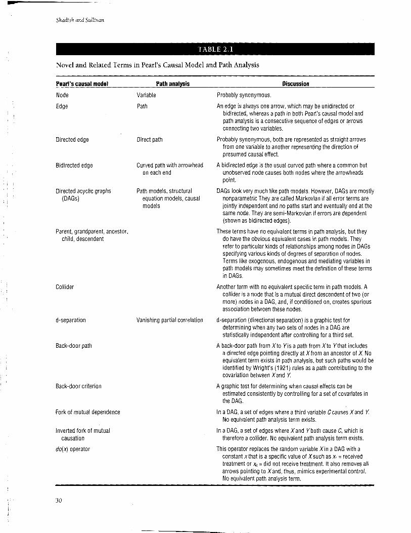
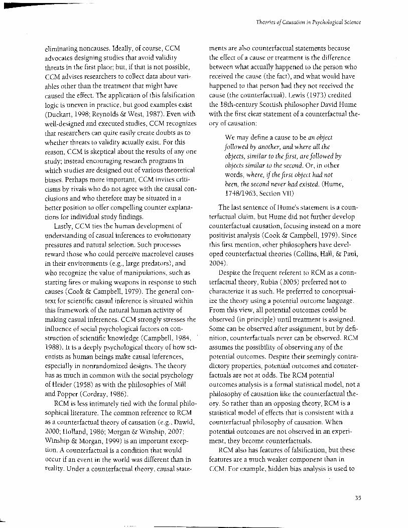
presentation of PCM relies heavily. For convenience given the number of new terms introduced in PCM, Table 2.1 summarizes some of the common terms in PCM and path analysis to clarify their overlap; readers familiar with path analysis may benefit from reading that table before continuing. New terms are italicized in text on first use.
PCM often works with graphs called directed acyclic graphs (DAGs). DAGs look like graphs that are common in path analysis, although they differ in important ways. The principles of PCM are based on nonparametric structural equation models (SEMs), augmented with ideas from both logic and graph theory. Yet PCM differs in important ways from SEM. Most implementations of SEM are parametric and require knowledge of the functional form of the relationships among all the variables in the model. PCM is nonparametric, so that one only need specify the relationships in the model, not whether the relationship between nodes is linear, quadratic, cubic, and so forth. PCM falls back on parametric modeling only when the nonparametric formulation of high dimensional problems is not practical. DAGs are Markovian, that is, they are acyclic in cases in which all the error terms in the DAG are jointly independent. PCM does not rely on these restrictions in many cases, however, when it allows correlation among error terms in the form of bidirected arrows or latent variables. DAGs may not include cycles (i.e., paths that start and eventually end at the same node). DAGs and PCM more generally do not assign any important role to the kinds of overall goodness-of-fit tests common to SEM, noting that support for a specific causal claim depends mostly on the theoretical assumptions embedded in the DAG that must be ascertained even if the model fits the data perfectly.
The starting point in PCM is the assertion that every exercise in causal analysis must commence with a set of theoretical or judgmental causal
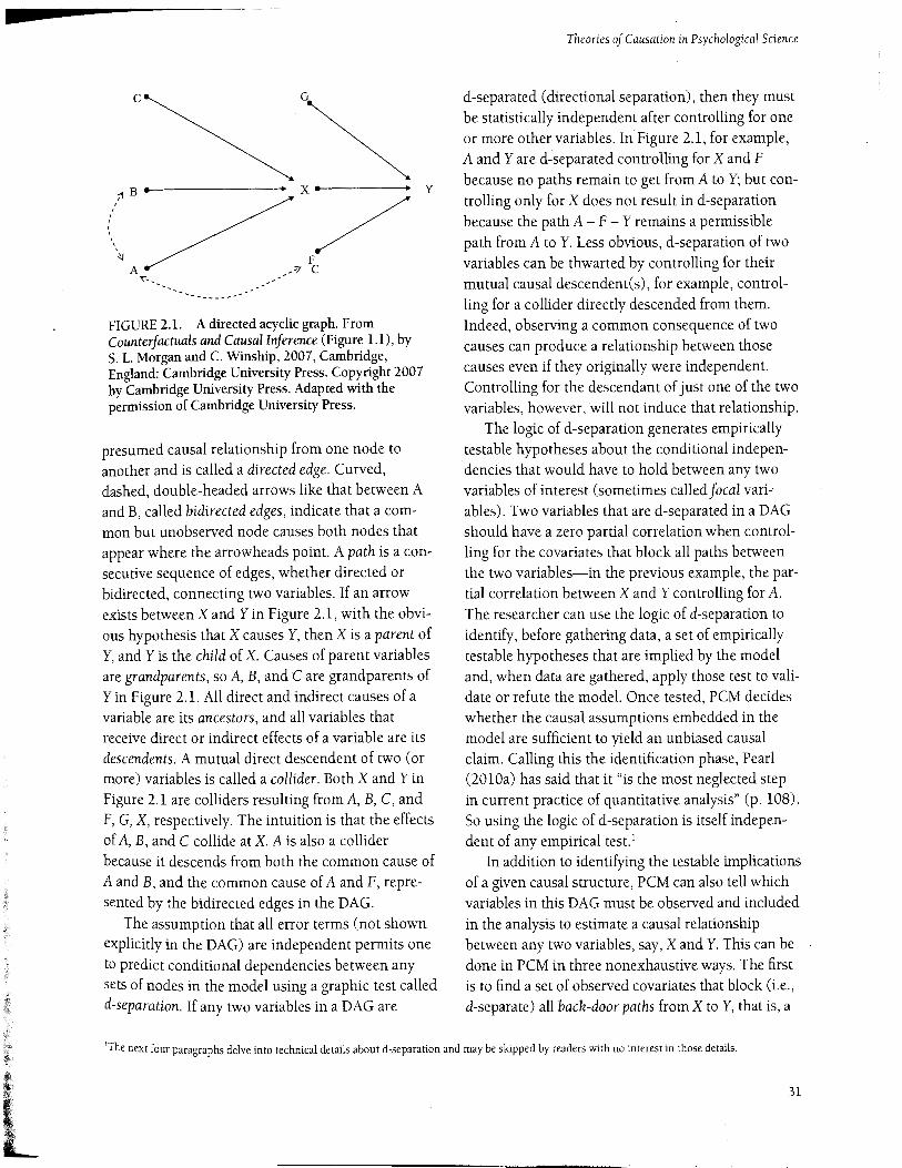
assumptions and that such assumptions are best articulated and represented in the form of directed acyclic graphs (DAGs). Consider Figure 2.1, for example. The letters each identify an observed random variable, called a node, represented by the solid black dot ( • ). A single-headed arrow like that going from X to Y indicates the direction of a
29
Shadish and Sullivan
TABLE 2.1
Novel and Related Terms in Pearl's Causal Model and Path Analysis
An edge is always one arrow, which may be unidirected or bidirected, whereas a path in both Pearl's causal model and path analysis is a consecutive sequence of edges or asrows connecting two variables.
Probably synonymous, both are represented as straight arrows from one variable to another representing the direction of presumed causal effect.
A bidirected edge is the usual curved path where a common but unobserved node causes both nodes where the arrowheads point.
DAGs look very much like path models. However, DAGs are mostly nonparametric They are called Markovian if all error terms are jointly independent and no paths start and eventually end at the same node. They are semi-Markovian if errors are dependent (shown as bidirected edges).
These terms have no equivalent terms in path analysis, but they do have the obvious equivalent cases in path models. They refer to particular kinds of relationships among nodes in DAGs specifying various kinds of degrees of separation of nodes. Terms like exogenous, endogenous and mediating variables in path models may sometimes meet the definition of these terms in DAGs.
Another term with no equivalent specific term in path models. A collider is a node that is a mutual direct descendent of two {or more) nodes in a DAG, and, if conditioned on, creates spurious association between these nodes.
d-separation (directional separation) is a graphic test for determining when any two sets of nodes in a DAG are statistically independent after controlling for a third set.
A back-door path from X to Yis a path from X to Ythat includes a directed edge pointing directly at X from an ancestor of X No equivalent term exists in path analysis, but such paths would be identified by Wright's (1921) rules as a path contributing to the covariation between X and Y.
A graphic test for determining when causal effects can be estimated consistently by controlling for a set of covariates in the DAG.
In a DAG, a set of edges where a third variable C causes X and Y. No equivalent path analysis term exists.
In a DAG, a set of edges where X and Yboth cause C, which is therefore a collider. No equivalent path analysis term exists.
This operator replaces the random variable X in a DAG with a constant xthat is a specific value of X such as x1 =received treatment or x0 = did not receive treatment. It also removes all arrows pointing to X and, thus, mimics experimental control. No equivalent path analysis term.
c
;'! 8
~
A '1:"--
G
X y
/ F
,"? c
FIGURE 2.1. A directed acyclic graph. From Counteifactuals and Causal Inference (Figure 1.1), by S. L. Morgan and C. Winship, 2007, Cambridge, England: Cambridge University Press. Copyright 2007 by Cambridge University Press. Adapted with the permission of Cambridge University Press.
presumed causal relationship from one node to another and is called a directed edge. Curved, dashed, double-headed arrows like that between A and B, called bidirected edges, indicate that a common but unobserved node causes both nodes that appear where the arrowheads point. A path is a consecutive sequence of edges, whether directed or bidirected, connecting two variables. If an arrow exists between X andY in Figure 2.1, with the obvious hypothesis that X causes Y, then X is a parent of Y, and Y is the child of X. Causes of parent variables are grandparents, so A, B, and Care grandparents of Yin Figure 2.1. All direct and indirect causes of a variable are its ancestors, and all variables that receive direct or indirect effects of a variable are its descendents. A mutual direct descendent of two (or more) variables is called a collider. Both X andY in Figure 2.1 are colliders resulting from A, B, C, and F, G, X, respectively. The intuition is that the effects of A, B, and C collide at X. A is also a collider because it descends from both the common cause of A and B, and the common cause of A and F, represented by the bidirected edges in the DAG.
The assumption that all error terms (not shown explicitly in the DAG) are independent permits one to predict conditional dependencies between any sets of nodes in the model using a graphic test called d-separation. If any two variables in a DAG are
Theories of Causation in Psychological Science
d-separated (directional separation), then they must be statistically independent after controlling for one or more other variables. In Figure 2.1, for example, A andY are d-separated controlling for X and F because no paths remain to get from A toY; but controlling only for X does not result in d-separation because the path A- F- Y remains a permissible path from A toY. Less obvious, d-separation of two variables can be thwarted by controlling for their mutual causal descendent(s), for example, controlling for a collider directly descended from them. Indeed, observing a common consequence of two causes can produce a relationship between those causes even if they originally were independent. Controlling for the descendant of just one of the two variables, however, will not induce that relationship.
The logic of d-separation generates empirically testable hypotheses about the conditional independencies that would have to hold between any two variables of interest (sometimes called focal vari-' ables). Two variables that are d-separated in a DAG should have a zero partial correlation when controlling for the covariates that block all paths between the two variables-in the previous example, the partial correlation between X andY controlling for A. The researcher can use the logic of d-separation to identify, before gathering data, a set of empirically testable hypotheses that are implied by the model and, when data are gathered, apply those test to validate or refute the model. Once tested, PCM decides whether the causal assumptions embedded in the model are sufficient to yield an unbiased causal claim. Calling this the identification phase, Pearl (2010a) has said that it "is the most neglected step in current practice of quantitative analysis" (p. 108). So using the logic of d-separation is itself independent of any empirical test. 1
In addition to identifying the testable implications of a given causal structure, PCM can also tell which variables in this DAG must be observed and included
in the analysis to estimate a causal relationship between any two variables, say, X andY. This can be done in PCM in three nonexhaustive ways. The first is to find a set of observed covariates that block (i.e., d-separate) all back-door paths from X toY, that is, a
'The next four paragraphs delve into technical details about d-separation and may be skipped by readers with no interest in those details.
31
Shadish and Sullivan
path from X to Y that includes a directed edge pointing directly at X from an ancestor of X. In Figure 2.1, the paths X- A- F- Y and X- B -A - F - Yare back-door paths. The directed edge from X to Yis not a back-door path because it contains no directed
edge pointing to X. One can identify a causal effect from X to Y by conditioning on observed variables that block each back-door path, in cases in which conditioning is done using standard control methods as stratification, matching, or regression with those variables. Conditioning on such variables in the graph is equivalent to satisfying the requirement of "strong ignorability" in the RCM (Pearl, 2009a, pp. 341-344).
Pearl (2000, 2009a) defined a variable or set of variables Z to block a back-door path if
l. the back-door path includes a mediational path from X toY (X---? C---? Y), where Cis in Z, or
2. the back-door path includes a fork of mutual dependence (X f- C---? Y), that is, where C causes X and Y, and C is in Z, or
3. the back-door path includes an inverted fork of mutual causation (X ---? C f- Y), where X and Y both cause C, and neither C nor its descendents are in Z.
The latter requirement means that Z cannot include a collider that happens to be on the backdoor path unless Z also blocks the pathways to that collider. According to these requirements, the backdoor paths from X to Yare blocked by conditioning on variables F or B A. Stratifying on A alone would not do because the backdoor path X- B -A- F- Y will remain unblocked.
The second strategy is to use an instrumental variable for X to estimate the effect of X on Y. In Figure 2.1, C is an instrument because it has no effect on Y except by its effect on X. Economists frequently
use this approach, and it assumes the effect of C on X and X on Yare both linear. The latter assumption
holds if C and X are dichotomous (e.g., a treatment dummy variable) andY is at least interval-scaled, both of which often hold in many observational studies. The estimate of the causal effect of X on Y is then the ratio of the effect of C on Y and X on Y. A problem would occur, however, if a directed edge from C to G is introduced into Figure 2.1. This
32
violates the definition of an instrument by creating a new back-door path from X toY through C and G. The causal estimate from X toY, however, still can be obtained by using C as an instrument while at the same time conditioning on G to block the back-door path-which also illustrates that these three strategies for estimating causal effects can be combined.
The third strategy is illustrated in Figure 2.2 where M and N have no parents other than X, and they also mediate the causal relationship between X and Y. The effect of X on Y can be estimated even if variables A and Fare unobserved, and the backdoor path X- A- F- Y remains unblocked. One estimates the causal effect of X on M and N, and then of M and N on Y, stratifying on X, and then combining the two estimates to construct the desired effect of X on Y. This can be done because M and N have no parents other than X in this DAG, so the effect of X on Y is completely captured by the mediators M and N.
PCM introduces the mathematical operator called do(x) to help model causal effects and counterfactuals. The operator do(x) mimics in the model what the manipulation of X can do in, say, a randomized experiment-that is, it can remove all paths into X. This operator replaces the random variable X in a DAG with a constant x that is a specific value of X such as x1 =received treatment or x0 = did not receive treatment. For instance, if we set X in Figure 2.1 to x0 , Figure 2.3 would result. Now
A F
-.:--_
FIGURE 2.2. A DAG with a mediating mechanism that completely accounts for the causal effect of X on Y. From Counteljactuals and Causal Inference (Figure 1.2), by S. L Morgan and C. Winship, 2007, Cambridge, England: Cambridge University Press. Copyright 2007 by Cambridge University Press. Adapted with the permission of Cambridge University Press.
c G
~ B '
X y
/ ' .:J F A
"="-----
FIGURE 2.3. A DAG figure from Figure 2.1 with a do(x) operator.
X is independent of all the variables that previously were its ancestors (A, B, and C), and no back-door paths exist. By comparing how results vary when setting x1 versus x0, PCM can emulate the effect of an intervention and express that effect mathematically, in terms of the (known and unknown) distributions that govern the variables in the graph. If that effect can be expressed in terms of observed distributions, the effect is identifiable, that is, it can be estimated without bias. Furthermore, the do(x)
operator in PCM does not require that X be manipulable. It can stand for a manipulable treatment, or a nonmanipulable treatment, such as gender, or the gravitational constant (Pearl, 2010a).
Three other points are implied by the preceding discussion. First, estimating causal effects does not require conditioning on all available variables; in many examples, a subset of these variables will suffice. In the case of an ancestral collider variable, conditioning should not be done. PCM provides rules for knowing which variables are sufficient, given the DAG, and which would be harmful. Second, when more than one of these three strategies can be applied to a given DAG, similar estimates from them may bolster confidence in the estimated effect conditional on the DAG. Third, the creation of a DAG leads to an explanatory model of causation, that is, a more elaborate depiction of the conditions under which, and mechanisms by which, X causes Y. So the DAG facilitates discussions among scientists to refine assumptions and confirm or refute their scientific plausibility. Morgan and Winship (2007), Hayduk et al. (2003), and Pearl (2000,
Theories of Causation in Psychological Science
2009a, 20l0a) have extensively elaborated these basic strategies and many other more complex examples.
PCM potentially enables the researcher to do many tasks. We have assumed the researcher is interested in only two focal variables, X and Yin our example; but the researcher may be interested in the causal effects of more than one pair of focal variables. For each pair of focal variables, the back-door paths, descendants, and control variables may differ, so in principle, the task becomes logistically more complex as more pairs of focal variables are of interest. Still, the DAG provides this information succinctly without having to remodel things from scratch when the focus changes. When the data are available, the researcher need not test the entire model at once, as is currently practiced, but rather can focus on the empirical implications of the model, keeping track of which tests are relevant to the target quantity, and which tests are more powerful or costly. A given causal claim might pass all the suggested tests, or some of them, or might not be testable for others. Hayduk et al. (2003) suggested that these tasks eventually will benefit from computer programs to conduct the tests and keep track of the results. Such programs are as yet in their infancy (Pearl, 2000, pp. 50-54; Scheines, Spines, Glymour, & Meek, 1994; Shipley, 2000, p. 306).
The most crucial matter in PCM is the creation of the DAG. The results of most of the logic and empirical tests of a DAG, and their implications for causal conclusions, depend on the DAG containing both the correct nodes and the correct set of edges connecting those nodes. These assumptions, in various disguises, must be made in every causal inference exercise, regardless of the approach one takes; hence the importance of making them explicit and transparent. This universal requirement is emphasized in numerous variants in PCM. For instance, in the pro
cess of discussing the relationship between PCM and Wright's (1921) work on path analysis, Pearl
(2010a) said, "Assuming of course that we are prepared to defend the causal assumptions encoded in the diagram" (p. 87). Still later in the same paper he said, "The lion's share of supporting causal claims falls on the shoulders of untested causal assumptions" (p. 35), and he regretted the current tendency
among propensity score analysts to "play down the
33
Shadish and Sullivan
cautionary note concerning the required admissibility of S" (p. 37). PCM asks researchers to do the homework necessary to create a plausible DAG during the design of the data-gathering study, recognizing, first, that this is likely to be a long-term iterative process as the scientific theory bolstering the DAG is developed, tested, and refined, and, second, that this process cannot be avoided regardless if one chooses to encode assumptions in a DAG or in many other alternative notational systems.
ANALYSIS OF THE THREE MODELS
We have now described the basic features of CCM, RCM, and PCM, and we move on to further compare and contrast the three models. Specifically, we address several of the models' core characteristics, including philosophies of causal inference, definitions of effect, theories of cause, external validity, matching, quantification, and emphases on design versus analysis. Finally, the chapter concludes with a discussion of some of the key problems in all these models.
Philosophies of Causal Inference RCM, CCM, and PCM have casual inference as their central focus. Consistently, however, CCM is more wide-ranging in its conceptual and philosophical scope; whereas RCM and PCM have a more narrow focus but also a more powerful formal statistical model. CCM courses widely through both descriptive and normative epistemological literature (Campbell, 1988; Shadish, Cook, & Leviton, 1991). This includes philosophy of causal inference (Cook & Campbell, 1986); but Campbell's epistemological credentials extend quite diversely into sociology of science, psychology of science, and general philosophy of science. For example, in the sociology of science, Campbell has weighed in on the merits of weak relativism as an approach to knowledge construction; in psychology of science, he discussed the social psychology of tribal leadership in science; and in the philosophy of science, Campbell coined the term evolutionary epistemology (Campbell, 1974) and is considered a significant contributor to that philosophical literature. Campbell's extensive
34
background in various aspects of philosophy of science thus brought an unusual wealth and depth to his discussions of the use of experiments as a way in which to construct knowledge in both science and day-to-day life.
CCM's approach to causation is tied more explicitly to the philosophical literature than RCM or PCM. For example, Cook and Campbell (1979) described their work as "derived from Mill's inductivist canons, a modified version of Popper's falsificationisfil, and a functionalist analysis of why cause is important in human affairs" (p. 1). CCM explicitly acknowledges the impact on Cook and Campbell's thinking of the work of the philosopher john Stuart Mill on causation. For instance, the idea that identifying a causal relationship requires showing that the cause came before the effect, that the cause covaries with the effect, and that alternative explanations of the relationship between the cause and effect are all implausible relates clearly to Mill's work. The threats to validity that CCM outline reflect these requirements. The threats to internal validity include Mill's first temporal requirement (ambiguous temporal precedence) and the remaining threats (history, maturation, selection, attrition, testing, instrumentation, regression to the mean) are examples of alternative explanations that must be eliminated to establish causation. CCM also acknowledges the influence of Mill's Methods of Experimental Inquiry (White, 2000). Certain design features are direct offshoots of this influence. For instance, CCM thinks about experimental methods not as identifying causes but rather eliminating noncauses (PCM sees this as a key feature of a DAG, as well), it acknowledges the distinct differences between casual inference from observation and casual inference by intervention, and it agrees that experimental inquiry methodology must be tailored to previous scientific knowledge as well as the real-world conditions in which the researcher is operating.
From philosopher Karl Popper (1959), CCM places the idea of falsifying hypotheses in a crucial role. Specifically, the model advises the experimenter to gather data that force causal claims to compete with alternative explanations epitomized by the threats to validity, complementing Mill's idea of
eliminating noncauses. Ideally, of course, CCM advocates designing studies that avoid validity threats in the first place; but, if that is not possible, CCM advises researchers to collect data about variables other than the treatment that might have caused the effect. The application of this falsification logic is uneven in practice, but good examples exist (Duckart, 1998; Reynolds & West, 1987). Even with well-designed and executed studies, CCM recognizes that researchers can quite easily create doubts as to whether threats to validity actually exist. For this reason, CCM is skeptical about the results of any one study; instead encouraging research programs in which studies are designed out of various theoretical biases. Perhaps more important, CCM invites criticisms by rivals who do not agree with the causal conclusions and who therefore may be situated in a better position to offer compelling counter explanations for individual study findings.
Lastly, CCM ties the human development of understanding of casual inferences to evolutionary pressures and natural selection. Such processes reward those who could perceive macro level causes in their environments (e.g., large predators), and who recognize the value of manipulations, such as starting fires or making weapons in response to such causes (Cook & Campbell, 1979). The general context for scientific casual inference is situated within this framework of the natural human activity of making casual inferences. CCM strongly stresses the influence of social psychological factors on construction of scientific knowledge (Campbell, 1984, 1988). It is a deeply psychological theory of how scientists as human beings make causal inferences, especially in nonrandomized designs. The theory has as much in common with the social psychology of Heider (1958) as with the philosophies of Mill and Popper (Cordray, 1986).
RCM is less intimately tied with the formal philosophical literature. The common reference to RCM as a counterfactual theory of causation (e.g., Dawid, 2000; Holland, 1986; Morgan & Winship, 2007; Winship & Morgan, 1999) is an important exception. A counterfactual is a condition that would occur if an event in the world was different than in reality. Under a counterfactual theory, causal state-
Theories of Causation in Psychological Science
ments are also counterfactual statements because the effect of a cause or treatment is the difference between what actually happened to the person who received the cause (the fact), and what would have happened to that person had they not received the cause (the counterfactual). Lewis (1973) credited the 18th-century Scottish philosopher David Hume with the first clear statement of a counterfactual theory of causation:
We may define a cause to be an object followed by another, and where all the objects, similar to the first, are followed by objects similar to the second. Or, in other words, where, if the first object had not been, the second never had existed. (Hume, 1748/1963, Section VII)
The last sentence of Hume's statement is a counterfactual claim, but Hume did not further develop counterfactual causation, focusing instead on a more positivist analysis (Cook & Campbell, 1979). Since this first mention, other philosophers have developed counterfactual theories (Collins, Hall, & Paul, 2004).
Despite the frequent referent to RCM as a counterfactual theory, Rubin (2005) preferred not to characterize it as such. He preferred to conceptualize the theory using a potential outcome language. From this view, all potential outcomes could be observed (in principle) until treatment is assigned. Some can be observed after assignment, but by definition, counterfactuals never can be observed. RCM assumes the possibility of observing any of the potential outcomes. Despite their seemingly contradictory properties, potential outcomes and counterfactuals are not at odds. The RCM potential outcomes analysis is a formal statistical model, not a philosophy of causation like the counterfactual theory. So rather than an opposing theory, RCM is a statistical model of effects that is consistent with a counterfactual philosophy of causation. When potential outcomes are not observed in an experiment, they become counterfactuals.
RCM also has features of falsification, but these features are a much weaker component than in CCM. For example, hidden bias analysis is used to
35
Shadish and Sullivan
falsify claimed effects by estimating how much bias (resulting from unmeasured variables) would have to be present before the effect's point and confidence interval changed. However, although this provides a change point, it does not tell whether hidden bias actually exists within the study. This can be an important point, as illustrated in a study described by Rosenbaum (1991) that seemed invulnerable to hidden biases. The study caused assignment probabilities ranging from .09 to .91; these probabilities cover almost the full range of possible nonrandom assignments (random assignment into two conditions with equal sample sizes would use a true probability of .50, to put this into context). According to Rosenbaum (1991), later research showed that a larger bias probably existed. In addition to bias assessment, propensity score analysis includes an examination of balance over groups after propensity score adjustment. If the data set is still extremely unbalanced, it is possible that the researcher will conclude that causal inference is not possible without heroic assumptions. This is a falsification of the claim that a causal inference can be tested well in the specific quasi-experiment. But these are minor emphases on falsification as compared with CCM, which is centrally built around the concept.
Although on the surface the philosophical differences between CCM and RCM appear quite numerous, practically no real disagreement results. For example, both models emphasize the necessity of manipulable experimental causes and advise against easy acceptance of proposed casual inference because of the fallibility of human judgment. It also is possible that they would agree on topics CCM addresses but RCM fails to mention. For instance, Cook and Campbell (1979) ended their discussion of causation with eight claims, such as "the effects in molar causal laws can be the results of multiple causes" (p. 33), and "dependable intermediate mediational units are involved in most strong molar laws" (p. 35). Although the specific statistical emphasis of RCM is not likely to have generated those claims, it is also unlikely that the model would disagree with any of them. Conversely, RCM philosophical writings are not extensive enough to generate true discord between the models.
36
The methodological machinery of PCM makes little explicit reference to philosophies of causation, but closer inspection shows both knowledge and use of them. The epilogue of Pearl (2000), for example, briefly reviewed the history of philosophy of causation, including Aristotle, David Hume, Bertrand Russell, and Patrick Suppes. Similarly, PCM acknowledges specific intellectual debts to Hume's framing of the problem of extracting causal inferences from experience (in the form of data) and to philosophical thinking on probabilistic causation (e.g., Eells, 1991). The most commonly cited philosophers in his book come mostly from the latter tradition or ones related to it, including not only Ellery Eels and Patrick Suppes but also Nancy Cartwright and Clark Glymour.
Where PCM differs most significantly from CCM and RCM is in its much greater emphasis on explanatory causation (the causal model within which X and Yare embedded) than descriptive causation (did X causeY?). This is not to say PCM is uninterested in the latter; clearly, all the rules ford-separation and do(x) operators are aimed substantially at estimating that descriptive causal relationship. Rather, it is that the mechanism PCM uses to get to that goal is quite different from RCM or CCM. The latter idealize the randomized experiment as the method to be emulated given its obvious strength in estimating the direct effect of X on Y. PCM gives no special place to that experiment. Rather, PCM focuses on developing a sufficiently complete causal model (DAG) with valid causal assumptions (about what edges are not in the model, in particular). In some senses, this is a more ambitious goal than in RCM or CCM, for it requires more scientific knowledge about all the variables and edges that must be (or not be) in the model. At its best, this kind of model helps to explain the observed descriptive causal relationship. Those explanations, in turn, provide a basis for more general causal claims, for they ideally can specify the necessary and sufficient conditions required for replicating that descriptive causal relationship in other conditions.
Possibly the most important difference in the philosophies of these three models is the greater stress on human (and therefore scientific) fallibility in CCM. Paradoxically, CCM is skeptical about the
L
possibility of performing tasks it sometimes requires to generate good causal inferences. Humans are poor at making many kinds of causal judgments, prone to confirmation biases, blind to apparent falsifications,
and lazy about both design and identifying alternative explanations. Yet when CCM's first line of defense, strong methodology and study design, either fails or is not practical to use, the next plan of attack often relies strongly on the above judgments to identify threats. Fallible human judgment is used to assess whether the identified threats have been rendered moot or implausible. This approach is especially true in weaker nonrandomized experiments. Because of the weight placed on human judgment, CCM argues that the responsibility to be critical lies within the community of scholars rather than with any one researcher, especially a community whose interests would lead them to find fault (Cook, 1985). As technology advances, tools such as propensity score analysis or DAGs sometimes can make it possible to substitute more objective measures or corrections for the fallible judgments.
Neither RCM nor PCM share the sweeping sense of fallibility in CCM. Yet they are self-critical in a different way. They focus less on the sense of fallibilism inherent in scientific work (as all scientists are also humans) and more on continually clarifying assumptions and searching for tests of assumptions. This results in many technical advances that reduce the reliance that CCM has on human judgment. For example, RCM emphasizes the importance of making and testing assumptions about whether a data set can support a credible propensity score analysis. PCM stresses the importance of careful and constant attention to the plausibility of a causal model. As of yet, however, the suggestions of PCM and RCM address only a fraction of the qualitative judgments made in CCM's wide-ranging scope.
Ironically, these senses of fallibilism are perhaps the hardest features of all three models to transfer
from theory into general practice. Many are the researchers who proudly proclaimed the use of a quasi-experimental design that Campbell would have found wanting. Many are the researchers who use propensity score analysis with little attention to
the plausibility of assumptions like strong ignorability. And many more may cite PCM as justification
Theories of Causation in Psychological Science
for causal inferences without the caveats about the plausibility of the model. As Campbell (1994) once said, "My methodological recommendations have been over-cited and under-followed" (p. 295).
Definition of Effect One of RCM's defining strengths is its explicit conceptual definition of an effect. In comparison, CCM never had an explicit definition of effect on a conceptual level until it adopted RCM's (Shadish et al., 2002). This is quite a substantial lapse given the centrality of finding the effects of causes within CCM. Implicitly, CCM defined effect using the counterfactual theory that RCM eschews in favor of the potential outcomes definition. The implicit definition governing CCM is most clearly outlined in Campbell's (1975) article "Degrees of Freedom and the Case Study," in which he addressed causal inference within a one-group pretest-posttest design. He supported using this type of design to infer effects only when substantial prior knowledge exists about how the outcome variable acts in the absence of the intervention, or in other words, with confident knowledge of the counterfactual.
Other than this example, however, CCM has treated effects as differences between two facts rather than two potential outcomes. For example, instead of thinking of it as the difference between what happened and what could have happened within one unit, CCM conceptualizes effects as what happened to the treatment group when compared with what happened to the control group, or what happened before treatment versus what happened posttreatment. This is not so much a conceptual definition of what effects are or should be in general as it is a computation to find observed differences. The computation worked reliably only in randomized experiments, and with other designs, it was considered valid only to the extent that the researcher was confident the quasi-experiment ruled out plausible alternative explanations, as randomized experiments can. In both models, then, the randomized experiment is upheld as the gold standard in design. RCM does so by building propensity score logic for nonrandomized studies on the basis of what is known about "regular" designs (Rubin, 2004), and CCM does so by acknowledging, as Campbell (1986)
37
I __ ,_,-
Shadish and Sullivan
noted, that "backhandedly, threats to internal validity were, initially and implicitly, those for which random assignment did control" (p. 68). CCM reaches the correct counterfactual only if those threats are implausible, and in this sense, threats to internal validity are counterfactuals. They are things that might possibly have happened if the treatment units had not received treatment. They are not all possible counterfactuals, however, as neither model has any way of fully knowing all possible counterfactuals.
Despite the fact that CCM has now incorporated RCM's definition of effect into its model, this is probably not enough. For example, CCM discusses why random assignment works (Shadish et al., 2002, Chapter 8), utilizing several explanations that are all partly true, but all of which might be better presented in the context of the potential outcomes model. Hypothetically then, CCM could present RCM's potential outcomes model, and then easily transition into how randomized experiments are a practical way in which to estimate the average causal effects that the model introduces on a conceptual level. Rubin (2005) has done the work for randomized experiments, and he and others have done the same for many nonrandomized experiments (e.g., Angrist & Lavy, 1999; Hahn, Todd, & Vander Klaauw, 2001; Morgan & Winship, 2007; Rubin, 2004; Winship & Morgan, 1999).
PCM's definition of effect relies on solving a set of equations representing a DAG to estimate the effect of X= x on Y, or more technically, to "the space of probability distributions on Y" (Pearl, 2000, p. 70), using the do(x) operator. Practically, this calculation most likely would be expressed as a regression coefficient, for example, from a SEM. This approach is more similar to how CCM would measure an effect than to RCM's definition of an effect. Yet PCM points out that it also can estimate a causal effect defined as the difference in the effect between the model where X= x0 and X= x1. The latter is neither a potential outcome nor a counterfactual definition of effect in RCM's sense because it is made on the basis of the difference between two estimates, whereas counterfactuals and potential outcomes cannot always be observed.
Most of CCM's approach to estimating effects could otherwise adopt the DAGs and associated
38
logic as a way of picturing effect estimation in their wide array of experimental and quasi-experimental designs. Probably the same is true of RCM. What most likely prevents such adoption is skepticism about two things. First, both RCM and CCM prefer design solutions to statistical solutions, although all three causal models use both. Second, both RCM and CCM have little confidence that those who do cause-probing studies in field settings can create an accurate DAG given the seemingly intractable nature of unknown selection biases. In their discussion of SEM, for example, Shadish et al. (2002) repeatedly stress the vulnerability of these models to misspecification. This remains one of the most salient differences between PCM on the one hand and RCM and CCM on the other.
Theory of Cause Of the three approaches, CCM has paid far more attention to a theory of cause than either RCM or PCM. This may occur for different reasons in PCM versus RCM. In the case of RCM, its focus on estimating effects in field settings requires practically no attention to the nature of causes: "The definition of 'cause' is complex and challenging, but for empirical research, the idea of a causal effect of an agent or treatment seems more straightforward or practically useful" (Little & Rubin, 2000, p. 122). In the case of PCM, its origins in mathematics, computer science, and graph theory may have given it a context in which causes were more often symbols or hypothetical examples than the kinds of complex social, educational, medical, or economic interventions in the real world that motivated RCM and CCM. If experiments really are about discovering the effects of manipulations, and if one's theory of causal inference is limited to experimental demonstrations that measure the effect, then this rudimentary definition of cause is possibly all that is needed. Even if it is not necessary, a more developed theory of cause still can be quite useful in understanding results.
The only knowledge we have about cause in an experiment often may be the actions the researcher took to manipulate the treatment. This is quite partial knowledge. CCM aspires to more, which is reflected specifically in the development of construct validity for the cause. For example, Campbell
(1957) stated that participant reactivity to the experimental manipulation is a part of the treatment; and he emphasized that experimental treatments are not single units of intervention, but rather multidimensional packages consisting of many components: "The actual X in any one experiment is a specific combination of stimuli, all confounded for interpretive purposes, and only some relevant to the experimenter's intent and theory" (p. 309). Cook and Campbell (1979) elaborated a construct validity of causes. Later work in CCM adopted Mackie's (1974) conception of cause as a constellation of features, of which researchers often focus on only one, despite the fact that all of the causes may be necessary to produce an effect (Cook & Campbell, 1986; Shadish et al., 2002). Furthermore, CCM stresses the necessity of programs of research to identify the nature and defining characteristics of a cause, using many studies investigating the same question, but with slight variations on the features of the causal package. This method will reveal some features that are crucial to the effectiveness of the causal package, whereas others will prove irrelevant. ·
To some extent, Campbell's interest in the nature of cause is a result of the context in which he worked: social psychology. Experiments in social psychology place high importance on knowing about cause in great detail because pervasive arguments often occur about whether an experimental intervention actually reflects the construct of interest from social psychology theory. By contrast, the highly abstract nature of PCM has not required great attention to understanding the cause; and applied experiments of the kind most common to RCM tend to be less theoretically driven than experiments in social psychology. But even those applied experiments could benefit from at least some theory of cause. For example, in the late 1990s, a team of researchers in Boston headed by the late Judah Folkman reported that a new drug called endostatin shrank tumors by limiting their blood supply (Folkman, 1996). Other respected researchers could not replicate the effect even when using drugs shipped to them from Folkman's lab. Scientists eventually replicated the results after they traveled to Folkman's lab to learn how to properly manufacture, transport, store, and handle the drug and how to inject it in the right location at
Theories of Causation in Psychological Science
the right depth and angle. An observer called these contingencies the "in-our-hands" phenomenon, saying, "Even we don't know which details are important, so it might take you some time to work it out" (Rowe, 1999, p. 732). The effects of endostatin required it to be embedded in a set of conditions that were not even fully understood by the original investigators and still may not be understood in the 21st century (Pollack, 2008).
Another situation in which a theory of cause is a useful tool is when considering the status of causes that are not manipulable. Both CCM and RCM agree that nonmanipulable agents cannot be causes within an experiment. CCM and PCM both entertain hypotheses about nonmanipulable causes, for instance, of genetics in phenylketonuria (PKU), despite the fact that the pertinent genes cannot be manipulated (Shadish et al., 2002). RCM is less clear on whether it would entertain the same ideas. This leads to debates within the field about the implications of manipulability for RCM and, more broadly, for the field of causal inference (Berk, 2004; Holland, 1986; Reskin, 2003; Woodward, 2003). Morgan and Winship (2007) made two points about this. First, it may be that RCM might not apply to causes that are not capable of being manipulated, because it is impossible to calculate an individual causal effect when the probability of a person being assigned to a condition is zero. Second, the counterfactual framework built into RCM encourages thinking about nonmanipulable causes to clarify the nature of the specific causal question being asked to specify the circumstances that have to be considered when defining what the counterfactual might have been. This is more complicated and ambiguous when dealing with nonmanipulable causes. For example, is the counterfactual for a person with PKU a person who is identical in every aspect except for the presence of the genetic defect from the moment it first appeared? Or, does it include a per-. son with every other result that the genetic defect could result in, such as the diet commonly used to treat PKU? PCM and CCM would consider all versions of these questions to be valid. PCM, for example, might devise multiple DAGs to represent each of the pertinent scenarios, estimating the causal effect for each.
39
Shadish and Sullivan
So CCM has a more functionally developed theory of cause than either PCM or RCM. This probably speaks again to the different goals the models have. CCM aspires to a generalized casual theory, one that covers most aspects (such as general cause theory) of the many kinds of inferences a researcher might make from various types of cause-probing studies. RCM has a much more narrow purpose: to define an effect clearly and precisely to better measure the effect in a single experiment. PCM has a different narrow purpose: to state the conditions under which a given DAG can support a causal inference, no matter what the cause. None of the three theories can function well without a theory of the effect; and all three could do without much theory of cause if effect estimation were the only issue. But this is not the case.
Causal Generalizations: External and Construct Validity CCM pays great attention to generalizability in the form of construct and external validity. Originally (e.g., Campbell, 1957; Campbell & Stanley, 1966), CCM merely identifies these concepts of generalization as important ("the desideratum"; Campbell & Stanley, 1966, p. 5), with little methodology developed for studying generalization except the multitrait-multimethod matrix for studying construct validity (Campbell & Fiske, 1959). Cook and Campbell (1979) extended the theory of construct validity of both the treatment and the outcome, and identified possible alternatives to random sampling that could be used to generalize findings from experiments. Cook (1990, 1991) developed both theory and methodology for studying the mechanisms of generalization, laying the foundation for what became three chapters on the topic in Shadish et al. (2002; Cook, 2004). Over the course of the 50 years this work spans, the theory and methodology have become more developed. For example, metaanalytic techniques now play a key role in analyzing
how effects vary over different persons, locations, treatments, and outcomes across multiple studies. Another important technique is identifying and modeling casual explanations that mediate between a cause and an effect; as such, explanations contextualize knowledge in a way that makes labeling and transferring the effect across conditions easier.
40
RCM has made contributions to meta-analysis and meditational modeling, both conceptual (e.g., Rubin, 1990, 1992) and statistical (e.g., Frangakis & Rubin, 2002; Rosnow, Rosenthal, & Rubin, 2000),
but the model rarely overtly ties these methods to the generalization of causes. One notable exception is Rubin's (1990, 1992) work on response surface modeling in meta-analysis. This work builds from the premise that a literature may not contain many or any studies that precisely match the metaanalyst's methodological or substantive question of interest. Rubin's approach to this problem is to use the available data from literature to project results to an ideal study that may not exist in literature but that would provide the test desired in a perfect world. This is a crucial form of external validity generalization; however, it has been little developed either statistically (Vanhonacker, 1996) or in application (Shadish, Matt, Navarro, & Phillips, 2000; Stanley &jarrell, 1998).
PCM has little to say explicitly about generalizations of any sort. To the extent that CCM is correct in its claim that causal explanation is a key facilitator of causal generalization, the DAGs in PCM are useful tools for the task if they are used to generate and test such explanations. An example might be the use of DAG technology to generate and test explanatory models of, say, causal mediation within randomized experiments. In addition, researchers who have a DAG and a data set against which to compare it can manipulate the operationalizations of the DAG to test various hypotheses that might bear on some generalizations. The logic would be similar to that of the do(x) operator, in which case the researcher fixes some variable to the value dictated by the desired generalization, for example, limiting the gender variable first to males and second to females, to test whether a treatment effect varies by gender.
Neither RCM nor CCM have been overly successful in translating their respective ideas and the
ory concerning causal generalizations into practical applications. This lack of success might be the result of the emphasis that is put on internal validity throughout applied scientific thinking and funding. An exception to this general rule is again meta-analysis, which has seen increased use and funding over the years. The increase in meta-analysis cannot be
L
directly credited to RCM or CCM, however. Rather, the increase seems to be focused on getting better effect size estimates instead of the more generalization-relevant exploration of how effects vary over person, treatment, or other study characteristics. In fact, a perusal of thousands of systematic reviews in the Cochrane Collaboration Library confirms that many meta-analyses include few or no tests of moderators that could be used for the latter aim, and these reviews report only the overall effect size for the intervention. The assumption among applied researchers seems to be that knowledge about causal generalization emerges fairly organically from programs of research and occasional reviews of them. Researchers appear to feel little need for active guid
ance on the topic. By contrast, the kinds of explanatory models that
PCM encourages are, in many respects, the heart of basic scientific theory. Scientists pursue those theories in multiple ways, from programs of research that explore moderators and mediators one at a time experimentally, to meditational models consistent with PCM. The main question would be whether the particular methods that PCM recommends are perceived by that community as having sufficiently novel and useful suggestions to warrant the effort to adopt them. The jury is still out on that question, perhaps not surprising given that PCM is the newest of the three theories.
Quantification Both PCM and RCM are much more thorough and successful in quantification than CCM. After all, Rubin is a statistician and Pearl is a computer scientist with an appointment in statistics. RCM has generated the highly quantitative potential outcomes model, pays careful attention to statistical assumptions, and has created statistical tools to improve effect estimation such as propensity scores and hidden bias analysis as well as other methodological
developments, such as the use of instrumental variable analyses in the presence of partial treatment implementation (Angrist et al., 1996). PCM has generated a theory of causal modeling with roots in mathematics, graph theory, and statistics, a theory that aspires to be the most general integration of the available quantitative approaches to causal inference.
Theories of Causation in Psychological Science
On the surface, it may not appear that CCM is quantitative given its more broad theoretical focus, but this is a bit deceiving. Few of the many students coming out of the tradition were quantitative (Brewer & Collins, 1981; Campbell, 1988), but notable exceptions have included Reichardt and Gollob (1986) and Trochim and Cappelleri (1992). Although Campbell himself was not a statistician, he successfully collaborated with the statisticians of his day for much of his work on specific methodology, such as regression discontinuity design (Cook, 2007) and the multitrait-multimethod matrix (Boruch & Wolins, 1970). The multitraitmultimethod matrix is not really a part of CCM, but regression discontinuity designs certainly are, and both lines of research are still pursued in the 21st century. In addition, CCM has attracted the attention of both statisticians and economists (Meyer, 1995; Meyer, Viscusi, & Durbin, 1995), although that attention often is critical (e.g., Cronbach, 1982; Rogosa, 1980).
Perhaps it is a more accurate assessment to say that CCM is quantitative on issues on the periphery of the CCM tradition. That is, CCM has given little attention to how to quantify matters that concern its validity typology, threats to validity, or how design features can be used to reduce the plausibility of threats. Fortunately, the omission of statistical applications within the theoretical framework is at least partially remediable. For example, much work has been done to quantify the effects of attrition on bias in randomized experiments, both within and outside of the CCM tradition (e.g., Deluccchi, 1994; Shadish, Hu, Glaser, Kownacki, & Wong, 1998; Shih & Quan, 1997; Verbeke & Molenberghs, 2000; Yeaton, Wortman, & Langberg, 1983). In addition, some work exists that quantifies the effects of testing threats to internal validity and outlines specific ways in which CCM could be more quantitative (Braver & Braver, 1988; Reichardt, 2000; Reichardt & Gollob,
1987; Solomon, 1949). Other research has been done to quantify CCM and join analysis to design, including the work by Winship and Morgan (1999) and Haviland, Nagin, and Rosenbaum (2007), which uses multiple pretests to improve inferences in nonrandomized designs. Clearly, CCM needs to begin to incorporate these developments more explicitly.
41
·--'-
Shadish and Sullivan
Quantification of CCM can only go so far because many issues concerning causation are more qualitative than quantitative. For example, one threat to internal validity is history, that is, an event not part of treatment occurred at the same time as treatment and was actually responsible for part or all of the observed effect. Another is the threat of instrumentation, for instance, a change in the instrument used to assess outcome across data points in a time-series design (Neustrom &. Norton, 1993). It is difficult to see how to include a covariate in a propensity score analysis that detects or adjusts for such threats, or to build those variables into a DAG. In addition, DAGS and propensity scores do little to assess threats to construct or external validity, and they are not designed to detect cases in which the qualitative and quantitative inferences differ, as when quantitative analysis suggests a treatment is effective, but an ethnographer identifies serious problems with it (Reichardt&. Cook, 1979). It is possible that the qualitative features of CCM eventually might be quantifiable in a grand statistical theory of causal inference. The breadth that this would necessarily cover makes it implausible that this will be developed in the near future. For this reason, the heavy focus of RCM and PCM on quantification necessitates that only a small subsection of casual theory is covered in these models. The parts that have been successfully quantified are the pieces connected most closely to the measurements of effects. These contributions are important but not sufficient on their own to assist the cause-probing researcher in all the pertinent tasks.
Design and Analysis Both RCM and especially CCM have a preference for strong designs, in particular randomized experiments, whenever possible. Except for matching designs, however, RCM focuses on analysis, and CCM focuses more on design. The best example of this difference is regression discontinuity design. Thistlethwaite and Campbell (1960) invented the design, but a statistical proof of the design was not published until Rubin (1977; an earlier unpublished proof was provided by Goldberger, 1972). Similarly, when time series are discussed in the RCM tradition (e.g., Winship&:. Morgan, 1999), such work focuses
42
entirely on analysis, whereas Campbell's treatment of the subject is much more design oriented. For example, CCM discusses such variations as adding a control group or nonequivalent dependent variable and using repeated and removed treatments, negative treatments, or staggered implementation across locations, which are aimed at increasing the confidence about any of the conclusions drawn about effects.
In most cases, these divergent emphases are quite complementary. CCM is strong on design and broad conceptual issues, but it lacks analytic sophistication as well as practical tools that move conclusions about confidence in effects from the qualitative to the quantitative realm when using a nonrandomized design. Conversely, RCM is strong on analysis, but some researchers utilize the statistical procedures without implementing careful design first, as both models would advocate. Yet the strengths of both models are essential: Good design makes for better analytic results, and better analyses can improve a potentially lower yield from a weak design. Examples of this are evident in the field; for instance, it is clear that tools like propensity scores can be used to remedy the reliance of CCM on qualitative judgments by scientists who often are not good at identifying and ruling out alternative casual explanations. Caution is necessary to implement the tools that RCM makes available, however. It can be tempting for scientists to take the lazy way out of difficult design issues and run less well-designed studies, hoping that the analytic tools can be used to fix bungled design.
RCM, like most statistical approaches to causation, appears to value design most when it contributes to a quantitative result (e.g., an effect size; confidence interval, or significance test). CCM expands on this approach and models how to use information even if it is only possible to do so in a qualitative fashion. For example, propensity score adjustment is an excellent tool to deal with a subset of threats to internal validity, namely, the selection threat and perhaps also maturation and regression, as special forms of selection bias. In this instance, the quantitative adjustment may be used to improve inferences about treatment effects. However, propensity score analysis does not address the internal
l
validity threats of history, testing, or instrumentation, despite the fact that all of these can produce a spurious effect. CCM accounts for this qualitatively and thus raises these concerns in a way that RCM does not. It would be best to have a way to quantify these concerns as well, but as of yet, neither CCM
nor RCM has done so. One noticeable exception to RCM's general pref
erence for analysis exists in the method of matching. Both CCM and RCM have considered the method of matching carefully, as it is frequently used as a seemingly plausible method for creating comparable groups when random assignment is not feasible. Until recently, CCM has maintained a generally skeptical stance toward matching in nonrandomized experiments, as evidenced in such comments as "the two groups have an inevitable systematic difference on the factors determining the choice involved, a difference which no amount of matching can remove" (Campbell, 1957, p. 300). The best-developed early study of this issue in CCM is that of Campbell and Erlebacher (1970), who analyzed the pernicious effects of matching on effect estimation in a study by Cicirelli and Associates (1969) concerning the effectiveness of the early Head Start program. The latter group of researchers presented startling results: that a matched group of children who did not receive the intervention performed better than the Head Start children. In response, Campbell and Erlebacher (1970) showed how the results actually could be due to a combination of selection bias on the true underlying variables and measurement unreliability. These problems together could have caused the groups to regress in opposite directions, thereby creating an inflated and invalid negative estimate of the treatment effect. This latter interpretation was supported by a reanalysis of the original data (Magidson, 1977). This event firmly embedded a general skepticism toward matching within the CCM tradition. More recently, however, CCM has relaxed the overarching skepticism and supported the use of matching on variables that are stable and reliable, such as achievement scores, aggregated to the school level and across years of pretest data (e.g., Millsap et al., 2000), and well-developed propensity scores.
Through the development of propensity scores, RCM has revived matching along with similar
Theories of Causation in Psychological Science
designs, such as stratification (Rubin, 2006). Because propensity scores are created by combining several covariates, they are more likely to be more stable and more reliable than the individual variables of which they consist. In this way, their use converges with the instances laid out by CCM in which matching is acceptable practice. The kinds of stable matching variables CCM originally endorsed were fairly uncommon, however, whereas propensity scores are more easily available. In addition, matching across propensity scores has clearer theoretical rationales for creating better estimates of effect. Despite this, in practice, results as to whether propensity scores actually do create better estimates seem to be mixed (Dehejia & Wahba, 1999; Glazerman, Levy, & Myers, 2003). Studies addressing this question with arguably better methodology, however, appear to be more optimistic (Luellen, Shadish, & Clark, 2005; Shadish, Clark, & Steiner, 2008; Shadish, Luellen, & Clark, 2006). Even in this latter group, however, propensity scores appear to be quite sensitive to how missing data in the covariates (that make up the score) are handled, quality of pretest covariate measurement might be more important than the specific statistics used to generate propensity scores, and research so far does not show a strong advantage of propensity scores over ordinary regression in reducing bias (e.g., Cook, Steiner & Pohl, 2009; Steiner, Cook, & Shadish, in press; Steiner, Cook, Shadish, & Clark, in press). Clearly, however, much more work needs to be done to identify the conditions under which one can be fairly confident that matching consistently reduces, rather than increases, bias.
Designs like randomized or nonrandomized experiments receive little attention in PCM, so it is difficult to know where PCM fits into this discussion. Nowhere in PCM does one find the granting of any special status to randomized experiments in estimating effects, although one might deduce from its discussion of the analogy between a do(x) operator and the physical operation of random assignment that PCM acknowledges the advantages of randomization for making causal estimation in a DAG easier to do. Discussions of randomized experiments in PCM tend to characterize them as a restricted paradigm because causal questions are
43
'i
Shadish and Sullivan
much broader than can be addressed by a randomized experiment.
Most of the prose in PCM is aimed at analysis, or at the conceptual work that goes into creating a DAG and a defensible causal claim before the analy
sis. That conceptual work might be considered a form of design in the same way that RCM considers attention to balancing tests before estimating effects to be a form of design. That is, both should occur without knowledge of the outcome analysis and should aim to set up the conditions to be met before a valid analysis of effects should occur. This is a much weaker form of design than present in CCM. Yet as a general conceptual structure, PCM can be adapted to any design and to the use of propensity score analysis and matching.
PCM has less enthusiasm for the kind of empirical comparisons of randomized to adjusted nonrandomized experiments that RCM and CCM have used to test, for example, whether propensity score adjustments in nonrandomized experiments yield the same answer as a parallel randomized experiment. Pearl (2010a) has noted that such tests provide no logical or mathematical proof of the similarity of the two methods and depend greatly on the particular context (setting, intervention, units, outcome measures, and perhaps even time) in which the study was run. Not surprisingly, then, we are aware of no empirical comparisons of effect estimates from randomized experiments versus an analysis based in PCM.
DISCUSSION
Discussing the relative merits of CCM, RCM, and PCM is made more difficult by substantial differences in terminology across the three theories. For example, imagine that CCM wishes to assess whether PCM or RCM give the same priority to internal validity that CCM does. Neither PCM nor RCM much mention that phrase, nor any of the other validity types and pertinent threats. Similarly, RCM's SUTVA is obtuse to many readers (Rubin, 2010; Shadish, 2010), with authors sometimes combining discussions of SUTV A with discussions of CCM's validity types in ways that perhaps neither RCM nor CCM would recognize or endorse (e.g.,
44
Dawid, 2000, p. 414; Oakes, 2004, p. 1943). And PCM has adopted a different language for talking about causation, so that the familiar terms in path analysis or structural equation modeling as used in CCM or RCM need translation into PCM terms that are not always cognates-a directed edge is not the same thing as a path, and not all structural equation models are direct~d acyclic graphs. These are, then, different models for approaching causation, and it is doubtful that any scholar has a sufficient grasp of all three to compare and evaluate them with full accuracy. In the present case, we are far more familiar with CCM than the other two models, and we are especially new to PCM. Still, the effort must be made to advance the interdisciplinary theory of causation that seems to be emerging in the past few decades.
One start to the comparison is to speculate about the key problems in each of the three models. Although the next three paragraphs will describe the problems in terms unique to each model, we will conclude that the problems all have a similar rootthey are all limited in one way or another by the state of knowledge about the key variables and the relationships among them. Starting with CCM, its concepts yield the broadest approach to causation of the three models. In particular, the attention to issues of construct and external validity are unmatched in the other two theories. Its key problem is its general lack of quantification, a point made by Rosenbaum (1999) in response to Shadish and Cook's (1999) early effort to compare parts of CCM to RCM. Threats to validity are central to CCM, for instance, yet CCM does not offer compelling quantitative ways to show how those threats affect an inference. Attrition is a good example, in part because it is a threat for which some quantitative work has been done (e.g., Deluccchi, 1994; Shadish et al., 1998; Shih & Quan, 1997; Verbeke & Molenberghs, 2000; Yeaton et al., 1983). Measuring attrition is simple; but CCM has no canonical method for showing what attrition rates result in a more or less accurate descriptive causal inference in a given study. Especially as applied in practice, many researchers simply note the amount of attrition that is present, and if it exceeds a subjectively formulated percentage, they allow that attrition may be a problem. Lack of quantification is to some
ji! __ _
degree inevitable in CCM given the breadth of its concepts, but it also results from a failure of many researchers within the CCM tradition even to try to
generate such answers. With RCM, two key problems emerge. One is the
pivotal role of the strong ignorability assumption, an assumption that so far cannot be tested within RCM yet that is absolutely central to the success of the methods that RCM suggests for observational studies. We have made only small steps in understanding how to select pretest covariates that might meet this condition (e.g., Cook et al., 2009; Steiner, Cook, &: Shadish, in press; Steiner, Cook, Shadish, &
Clark, in press). PCM asserts that it has completely solved this problem in theory, to the maximum extent allowed by available scientific knowledge, yet the available knowledge in many practical endeavors is so scant that we are skeptical whether one can take full advantage of this solution. The second problem is its failure, at least until recently, to give sufficient attention to the design of good observational studies. Most of the early examples that RCM gave relied on observational data sets that already has been gathered by other researchers for other purposes, with RCM doing a secondary analysis to
try to improve the accuracy of the effect estimate. Only in the past few years has RCM begun to write about the importance of good prospective design of observational studies: both the use of better design elements like carefully selected control groups, and the deliberate development of measures of the selection process through such means as interviewing participants and providers to discover and accurately describe those processes (Rubin, 2007, 2008).
Two key problems also emerge with PCM. The first is the necessity in PCM of knowing that the DAG is correct, for otherwise the results of the logical and empirical tests in PCM may be incorrect. A mature research topic sometimes may be confident of the key variables and the relationships among them, especially if the problem is investigated in a closed system with a limited number of variables known to be relevant. Some parts of cognitive science might approximate these conditions, for example. The applied causal questions of most interest to RCM and CCM, however, almost certainly do not do so. As a corollary, then, PCM's approach to strong
Theories of Causation in Psychological Science
ignorability also relies on correct specification of the DAG, with the same implications of an incorrect DAG for the accuracy of the test. The second problem is the paucity of examples of practical applications of PCM. This may in part be what Imbens (2010) referred to when he said,
My personal view is that the proponents of the graphical approach ... have not demonstrated convincingly to economists that adopting (part) of their framework offers sufficient benefits relative to the framework currently used by economists. (p. 4 7)
Morgan and Winship (2007) have provided some examples, but their book so thoroughly mixes RCM and PCM that the benefits specific to PCM are not necessarily transparent. Indirect evidence of the potential usefulness of PCM is the fact that many economists and social scientists use structural equation models that are closely related to DAGs, despite lingering difficulties in interpreting their causal content (difficulties that PCM claims to have eliminated).
One common theme across the problems in all three theories is that despite the different ways that each theory has approached causal inference, in observational studies, one must make assumptions of some sort to make progress. With CCM, it is the assumption that the researcher has ruled out threats to validity (alternative explanations for the effect); with RCM, it is the assumption that strong ignorability holds; and, with PCM, it is the assumption that the DAG is correct. In all three, of course, one can use data or logic or experience to probe the validity of these assumptions, measuring some of the threats to see whether they remain plausible, showing that one obtains balance with propensity scores, or showing that the DAG is consistent with the observed data or past research. But these are profoundly fallible probes, they only test parts of the relevant assumptions or are only weakly related to the assumption, and they are incapable in principle of proving the assumptions are valid. With observational studies, we have no free lunch, no royal road to valid effect estimation.
PCM claims to offer some visibility from this treacherous road. For example, it claims that a recent
45
--
Shadish and Sullivan
proof of the completeness of the "do-calculus" (Shpitser & Pearl, 2008) implies that no method can do better than PCM, given the same uncertainty about the science underlying a problem. For PCM, Halpern's (1998) proof that RCM and PCM are logically equiva
lent, differing merely in emphasis and convenience, further implies that an informative comparison between the two should examine separately each phase of the inference process (as was done in Pearl, 2010b). PCM aims to demonstrate the benefit of a hybrid strategy whereby scientific knowledge is articulated via graphs, and algebraic derivations are pursued in RCM notation. But this is difficult to do correctly.
Herein lies a dilemma. PCM requires knowledge of two things: (a) the right set of variables and (b) the right model of the relationship between those variables. For many or perhaps nearly all applications that might be characterized by such terms as program evaluation or applied quasi-experimentation or cognates, most researchers regard the first task as nearly hopeless given how unknown selection bias typically is. To aspire to the second task if the first one is hopeless seems not only doubly hopeless but also more time-consuming than the benefits likely will warrant. This suggests a complementary interpretation to that oflmbens (2010), that a failure to adopt PCM to these applied problems reflects a justifiable skepticism about the value of the additional work.
RCM's program of research seems aimed at the first of these two tasks in hopes that its tools like propensity score adjustment might be able to do good enough in making correct causal assessments from observational data. Consider, for example, recent empirical efforts to understand the conditions under which statistical adjustments of quasi-experiments can be made to match findings from randomized experiments (e.g., Cook, Shadish, & Wong, 2008; Cook et al., 2009; Dehejia & Wahba, 1999; Glazerman et al., 2003; Shadish et al., 2008; Steiner, Cook, & Shadish, in press; Steiner, Cook, Shadish, & Clark, in press). One might think of such studies as a program of research conducted on the basis of induction. Such studies take existing suggestions for improving causal estimates, such as propensity score analysis or the use of DAG methods, and test those suggestions empirically. No single test of this kind can escape its context, so any generalizations from
46
one such a study would be extremely speculative. But a program of research of this kind, where multiple investigators vary many key features of the study (persons, settings, times, treatments, outcomes, etc.), has the potential to produce an empiri
cal basis for making inductive hypotheses about what does and does not work in generating accurate causal estimates. Given the problem of induction (that we may never know if we will observe a falsifying instance), such results never can be logically conclusive. Indeed, we cannot rule out the possibility that the program will fail to identify any useful hypotheses. If such a program were to be successful, however, it would help us to understand the conditions under which we might be able to create causal estimates that are good enough (accurate enough by some criterion to be agreed on by the community of scholars), albeit not optimal. This is a different approach from PCM's provision of a causal logic that allows the researcher to deduce causal inferences from a given set of conditions, a more challenging task but one that eventually might lead to a solution more likely to be optimal if it could be successful.
CCM falls in between the other two models in its approach to this dilemma, but probably with more affinity to RCM than PCM. On the one hand, CCM always has allowed that if you fully know the specification of the selection process and measure that process perfectly, then the researcher can use methods like structural equation modeling to generate accurate causal estimates. Adding the benefits of PCM's approach to this claim would probably strengthen CCM's understanding and explication of the conditions under which this can be done. On the other hand, CCM shares the skepticism of RCM about being able to solve PCM's second task. Ultimately, CCM prefers advocating stronger experimental and quasi-experimental design approaches that are less formalized and more reliant on fallible but inevitable plausibility judgments; and CCM takes the inductive program of research as its best current hope for solving the applied causal inference problems of most interest to CCM and RCM.
We can give two reasonable responses to these reservations, however. First, we must make the effort to do both tasks if we really want to advance scientific and practical understanding of what
-
L
works. After all, if we do not try to model the relationships among variables in a serious way now, then when should we do so? Should we wait for the
inductive program to reach its limits or fail? Should we pursue both inductive and deductive tasks simultaneously, and if so, what incentive is there for applied researchers to take on the harder task? Surely, however, we should not simply abandon the second task just because it is harder to do both tasks
than just the first. The second reasonable response is that PCM has
identified some specific conditions under which adjusting for certain pretest variables, whether in propensity scores or ordinary regression, can increase bias of causal estimates. The most salient of them is the collider variable, a variable that is a mutual direct descendent of two (or more) variables, which if controlled can increase bias. A second example is certain uses of instrumental variables that might also increase bias (Pearl, 2009b). A useful project would be to begin to identify and catalog such conditions, probably separately for each substantive area of interest. The project is formidable because knowing that a variable is an instrument or a collider depends on knowing the relationships among variables. But the project is probably not impossible to begin.
Most likely, we need multiple approaches to solving these difficult causal inference issues. We need the inductivist investigators who use results from many studies to create a theory of when tools like propensity score analysis might help. We need the deductivist investigators who will create the SEMs and DAGs that better embody the goals of science involving creation of better scientific theories about the phenomena we study. Who will do each kind of research will no doubt depend on many fac
tors, including but not limited to a researcher's perception of whether the knowledge base in a field is mature enough to support strong model develop
ment and whether the perceived payoff of investing resources into doing each task compared with the alternatives is worth the effort.
Elsewhere we have described other gaps in RCM and CCM (Shadish, 2010). PCM helps fill some but not all of those gaps. One was that CCM and RCM both focus primarily on field experimentation. PCM
Theories of Causation in Psychological Science
may connect a bit better to laboratory experimentation in which tight experimental control and careful attention to theoretically based construction of causal models might make a DAG more likely to be plausible. A second gap was that RCM and CCM both focus somewhat more on the simple descriptive inference that A caused B, and less so on the explanatory mediators and moderators of the effect. Again PCM attends more to the latter as a by-product of the construction of a valid DAG. A third gap is that all of these three theories devote far more attention to finding the effects of known causes than to finding the unknown causes of known effects. PCM has put the most effort of the three into creating fully developed theories of causes of effects, including attribution, regret, explanation, and other counterfactual relationships (see Pearl, 2009a, Chapters 9 and 10). The latter is often the province of epidemiology, especially retrospective case control studies. Perhaps a further iteration of this comparison of theories of causation might include the work of james Robins, and epidemiologist and biostatistician whose work might help fill this gap (e.g., Robins, Hernan, & Brumback, 2000).
What is encouraging about all these developments, however, is the possible emergence of a truly interdisciplinary theory of causation applied to the conduct of social science (lmbens, 2010). Many economists and statisticians have begun to use the common terminology supplied by the potential outcomes model in RCM to talk about causation (e.g., Angrist et al., 1996). Statisticians have begun to write much more about the importance of good design and pretest measurement to the statistical adjustments they suggest (Rubin, 2007, 2008). Psychologists have begun to incorporate analytic models from RCM into their work (Shadish et al., 2002, 2008). Sociologists have combined RCM and PCM in a synthesis that also includes more extensive discussion of good design (Morgan & Winship, 2007).
Because of the sheer number of disciplines involved, and the many terminological differences across PCM, CCM, and RCM (and others), the going is slow and the progress is incremental, measured in decades. But progress it is, and a shared theory of causal inference that moves beyond CCM, RCM, and PCM does now indeed seem feasible.
47
.',[
Shadish and Sullivan
References Angrist,J. D., Imbens, G. W., & Rubin, D. B. (1996).
Identification of causal effects using instrumental variables. journal of the American Statistical Association, 91, 444-455. doi:10.2307/2291629
Angrist,j. D., & Lavy, V. (1999). Using Maimonides' rule to identify the effects of class size on scholastic achievement. The Quarterly journal of Economics, 114, 533-575. doi:10.1162/003355399556o61
Berk, R. A. (2004). Regression analysis: A constructive critique. Thousand Oaks, CA: Sage.
Boruch, R. F., & Wolins, L. (1970). A procedure for estimation of trait, method, and error variance attributable to a measure. Educational and Psychological Measurement, 30, 547-574.
Braver, M. C. W., & Braver, S. L. (1988). Statistical treatment of the Solomon Four-Group design: A meta-analytic approach. Psychological Bulletin, 104, 150-154. doi: 10.1037/0033-2909.104.1.150
Brewer, M. B., & Collins, B. E. (Eds.). (1981). Scientific inquiry and the social sciences: A volume in honor of Donald T. Campbell. San Francisco, CA: Jossey-Bass.
Burns, M., & Pearl,]. (1981). Causal and diagnostic inferences: A comparison of validity. Organizational Behavior and Human Performance, 28, 379-394. doi: 10.1016/0030-5073(81)90005-2
Campbell, D. T. (1957). Factors relevant to the validity of experiments in social settings. Psychological Bulletin, 54, 297-312. doi:10.1037/h0040950
Campbell, D. T. (1974). Evolutionary epistemology. In P. A. Schilpp (Ed.), The philosophy of Karl Popper (pp. 412-463). La Salle, IL: Open Court.
Campbell, D. T. (1975). "Degrees of freedom" and the case study. Comparative Political Studies, 2, 178-193.
Campbell, D. T. (1984). Toward an epistemologically relevant sociology of science. Science, Technology, and Human Values, 10, 38-48.
Campbell, D. T. (1986). Relabeling internal and external validity for applied social scientists. In W. M. K. Trochim (Ed.), Advances in quasi-experimental design and analysis (pp. 67-77). San Francisco, CA: JosseyBass.
Campbell, D. T. (1988). Methodology and epistemology for social science: Selected papers (E. S. Overman, Ed.). Chicago: University of Illinois Press.
Campbell, D. T., & Erlebacher, A. E. (1970). How regression artifacts can mistakenly make compensatory education programs look harmful. In]. Hellmuth (Ed.), The Disadvantaged Child: Vol. 3. Compensatory education: A national debate. New York, NY: Bruner/ Mazel.
48
Campbell, D. T., & Fiske, D. W. (1959). Convergent and discriminant validation by the multitraitmultimethod matrix. Psychological Bulletin, 56, 81-105. doi:10.1037/h0046016
Campbell, D. T., & Stanley,]. C. (1963). Experimental and quasi-experimental designs for research on teaching. InN. L. Gage (Ed.), Handbook of research on teaching (pp. 171-246). Chicago, IL: Rand McNally.
Campbell, D. T., & Stanley,]. C. (1966). Experimental and quasi-experimental designs for research. Chicago, IL: Rand McNally.
Chapin, F. S. (1932). The advantages of experimental sociology in the study of family group patterns. Social Forces, 11, 200-207. doi:10.2307/2569773
Chapin, F. S. (194 7). Experimental designs in sociological research. New York, NY: Harper.
Cicirelli, V. G., & Associates. (1969). The impact of Head Start: An evaluation of the effects of Head Start on children's cognitive and affective development: Vol. 1. A report to the Office of Economic Opportunity. Athens: Ohio University and Westinghouse Learning Corporation.
Collins,]., Hall, E., & Paul, L. (Eds.). (2004). Causation and counterfactuals. Cambridge, MA: MIT Press.
Cook, T. D. (1985). Postpositivist critical multiplism. In L. Shotland & M. M. Mark (Eds.), Social science and social policy (pp. 21-62). Newbury Park, CA: Sage.
Cook, T. D. (1990). The generalization of causal connections: Multiple theories in search of clear practice. In L. Sechrest, E. Perrin, &J. Bunker (Eds.), Research methodology: Strengthening causal interpretations of nonexperimental data (pp. 9-31) (DHHS Publication No. PHS 90-3454). Rockville, MD: Department of Health and Human Services.
Cook, T. D. (1991). Clarifying the warrant for generalized causal inferences in quasi-experimentation. In M. W. Mclaughlin & D. C. Phillips (Eds.), Evaluation and education: At quarter-century (pp. 115-144). Chicago, IL: National Society for the Study of Education.
Cook, T. D. (2004). Causal generalization: How Campbell and Cronbach influenced my theoretical thinking· on this topic, including in Shadish, Cook, and Campbell. In M. Alkin (Ed.), Evaluation roots: Tracing theorists' views and influences (pp. 88-113). Thousand Oaks, CA: Sage.
Cook, T. D. (2007). "Waiting for life to arrive": A history of the regression-discontinuity design in psychology, statistics and economics. journal of Econometrics, 142, 636-654. doi: 10.1016/j.jeconom.2007.05.002
Cook, T. D., & Campbell, D. T. (1979). Quasiexperimentation: Design and analysis issues for field settings. Chicago, IL: Rand McNally.
Cook, T. D., & Campbell, D. T. (1986). The causal assumptions of quasi-experimental practice. Synthese, 68, 141-180.
Cook, T. D., Shadish, W. R., & Wong, V. C. (2008). Three conditions under which experiments and observational studies produce comparable causal estimates: New findings from within-study comparisons. Journal of Policy Analysis and Management, 2 7, 724-750. doi: 10.1002/pam.203 75
Cook, T. D., Steiner, P.M., & Pohl, S. (2009). How bias reduction is affected by covariate choice, unreliability, and mode of data analysis: Results from two types of within-study comparisons. Multivariate Behavioral Research, 44, 828-84 7. doi: 10.1080/002 731709033336 73
Cordray, D. W. (1986). Quasi-experimental analysis: A mixture of methods and judgment. In W. M. K. Trochim (Ed.), Advances in quasi-experimental design and analysis (pp. 9-27). San Francisco, CA: josseyBass.
Cronbach, L.]. (1982). Designing evaluations of educational and social programs. San Francisco, CA: jossey-Bass.
D'Agostino, R.,jr., & Rubin, D. B. (2000). Estimation and use of propensity scores with incomplete data. Journal of the American Statistical Association, 95, 749-759. doi:10.2307/2669455
Dawid, A. P. (2000). Causal inference without counterfactuals. Journal of the American Statistical Association, 95, 407-448. doi:10.2307/2669377
Dehejia, R., & Wahba, S. (1999). Causal effects in nonexperimental studies: Re-evaluating the evaluation of training programs. Journal of the American Statistical Association, 94, 1053-1062. doi:10.2307/2669919
Deluccchi, K. L. ( 1994). Methods for the analysis of binary outcome results in the presence of missing data. Journal of Consulting and Clinical Psychology, 62, 569-575. doi:10.1037/0022-006X.62.3.569
Duckart,]. P. (1998). An evaluation of the Baltimore Community Lead Education and Reduction Corps (CLEARCorps) Program. Evaluation Review, 22, 373-402. doi:10.1177/0193841X9802200303
Eells, E. (1991). Probabilistic causality. New York, NY: Cambridge University Press. doi:10.1017/ CB09780511570667
Fisher, R. A. (1925). Statistical methods for research workers. London, England: Oliver & Boyd.
Fisher, R. A. (1926). The arrangement of field experiments. Journal of the Ministry of Agriculture, 33, 503-513.
Folkman,]. (1996). Fighting cancer by attacking its blood supply. Scientific American, 275, 150-154. doi: 10 .1038/scientificamerican0996-150
Theories of Causation in Psychological Science
Frangakis, C., & Rubin, D. B. (2002). Principal stratification in causal inference. Biometrics, 58, 21-29. doi: 10.1111/j.0006-341X.2002.00021.x
Frangakis, C. E., Rubin, D. B., & Zhou, X.-H. (2002). Clustered encouragement designs with individual noncompliance: Bayesian inference with randomization, and applications to advanced directive forms. Biostatistics (Oxford, England), 3, 147-164. doi: 10.1093/biostatistics/3.2.14 7
Freedman, D. A. (1987). As others see us: A case study in path analysis. Journal of Educational Statistics, 12, 101-128. doi:10.2307/1164888
Glazerman, S., Levy, D. M., & Myers, D. (2003). Nonexperimental versus experimental estimates of earnings impacts. The Annals of the American Academy of Political and Social Science, 589, 63-93. doi:10.1177/0002716203254879
Goldberger, A. S. (1972). Selection bias in evaluating treatment effects: Some formal illustrations (Discussion Paper 123-72). Madison: University of Wisconsin, Institute for Research on Poverty.
Hahn,]., Todd, P., & Vander Klaauw, W. (2001). Identification and estimation of treatment effects with a regression-discontinuity design. Econometrica, 69, 201-209. doi: 10.1111/1468-0262.00183
Halpern,]. Y. (1998). Axiomatizing causal reasoning. In G. F. Cooper & S. Moral (Eds.), Uncertainty in artificial intelligence (pp. 202-210). San Francisco, CA: Morgan Kaufmann.
Haviland, A., Nagin, D. S., & Rosenbaum, P.R. (2007). Combining propensity score matching and group-based trajectory analysis in an observational study. Psychological Methods, 12, 247-267. doi: 10.1037 /1082-989X.12.3.24 7
Hayduk, L., Cummings, G., Stratkotter, R., Nimmo, M., Grygoryev, K., Dosman, D., ... Boadu, K. (2003). Pearl's D-Separation: One more step into causal thinking. Structural Equation Modeling, 10, 289-311. doi: 10.1207 /S15328007SEM1002_8
Heider, F. (1958). The psychology of interpersonal relations. New York, NY: Wiley.
Holland, P. W. (1986). Statistics and causal inference. Journal of the American Statistical Association, 81, 945-970. doi: 10.2307/2289064
Hume, D. (1963). An enquiry concerning human understanding. LaSalle, IL: Open Court Press. (Original work published 1748)
Imbens, G. W. (2010). An economist's perspective on Shadish (2010) and West & Thoemmes (2010). Psychological Methods, 15, 47-55.
Lazarsfeld, P. F. (1948). The use of panels in social research. Proceedings of the American Philosophical Society, 92, 405-410.
49
Shadish and Sullivan
Lewis, D. (1973). Counterfactuals. Cambridge, MA: Blackwell.
Light, R.j., Singer,]. D.,&:: Willett,]. B. (1990). By design: Planning research in higher education. Cambridge, MA: Harvard University Press.
Little, R.j. A.,&:: Rubin, D. B. (2000). Causal effects in clinical and epidemiological studies via potential outcomes: Concepts and analytic approaches. Annual Review of Public Health, 21, 121-145. doi:10.ll46/ annurev.publhealth.2l.l.12l
Little, R.]. A.,&:: Rubin, D. B. (2002). Statistical analysis with missing data (2nd ed.). New York, NY: Wiley.
Luellen,]. K., Shadish, W. R., &:: Clark, M. H. (2005). Propensity scores: An introduction and experimental test. Evaluation Review, 29, 530-558. doi:lO.ll77/ 0193841X05275596
Mackie,]. L. (1974). The cement of the universe: A study of causation. Oxford, England: Oxford University Press.
Magidson,j. (1977). Toward a causal model approach for adjusting for preexisting differences in the nonequivalent control group situation. Evaluation Quarterly, 1, 399-420. doi:lO.ll77/0193841X7700100303
McCall, W. A. (1923). How to experiment in education. New York, NY: Macmillan.
Meyer, B. D. (1995). Natural and quasi-experiments in economics. journal of Business and Economic Statistics, 13, 151-161. doi:l0.2307/l392369
Meyer, B. D., Viscusi, W. K., &:: Durbin, D. L. (1995). Workers' compensation and injury duration: Evidence from a natural experiment. The American Economic Review, 85, 322-340.
Millsap, M.A., Chase, A., Obeidallah, D., Perez-Smith, A. P., Brigham, N., &Johnston, K. (2000). Evaluation of Detroit's Comer Schools and Families Initiative: Final REPORT. Cambridge, MA: Abt Associates.
Morgan, S. L., &:: Winship, C. (2007). Counterfactuals and causal inference. Cambridge, England: Cambridge University Press.
Neustrom, M. W., & Norton, W. M. (1993). The impact of drunk driving legislation in Louisiana. journal of Safety Research, 24, 107-121. doi: 10.1016/0022-4375(93)90005-8
Neyman,]. (1990). On the application of probability theory to agricultural experiments: Essay on principles. Section 9. Statistical Science, 5, 465-480. (Original work published 1923)
Oakes,]. M. (2004). The (mis)estimation of neighborhood effects: Causal inference for a practicable social epidemiology. Social Science and Medicine, 58, 1929-1952. doi:10.l016/j.socscimed.2003.08.004
Pearl,]. (1998). Graphs, causality, and structural equation models. Sociological Methods and Research, 27, 226-284. doi:lO.ll77/0049124198027002004
50
Pearl,]. (2000). Causality: Models, reasoning, and inference. New York, NY: Cambridge University Press.
Pearl,]. (2009a). Causality: Models, reasoning, and inference (2nd ed.). New York, NY: Cambridge University Press.
Pearl,]. (2009b). On a class of bias-amplifying covariates that endanger effect estimates (Technical Report R-356). Retrieved from http://ftp.cs.ucla.edu/pub/ stat_ser/r356.pdf
Pearl,]. (20 lOa). The foundations of causal inference. Sociological Methodology, 40, 74-149. doi:lO.ll1ll j.1467 -953l.2010.01228.X
Pearl,]. (20l0b). An introduction to causal inference. The International]ournal of Biostatistics, 6. doi:10.2202/1557-4679.l203
Pearl,].,&:: Tarsi, M. (1986). Structuring causal trees. journal of Complexity, 2, 60-77. doi:10.l016/0885-064X(86)90023-3
Pollack, A. (2008,]anuary 28).judah Folkman, researcher, dies at 74. New York Times. Retrieved from http://www.nyt.com
Popper, K. R. (1959). The logic of scientific discovery. New York, NY: Basic Books.
Reichardt, C. S. (2000). A typology of strategies for ruling out threats to validity. In L. Bickman (Ed.), Research design: Donald Campbell's legacy (Vol. 2, pp. 89-115). Thousand Oaks, CA: Sage.
Reichardt, C. S., &:: Cook, T. D. (1979). Beyond qualitative versus quantitative methods. InT. D. Cook&:: C. S. Reichardt (Eds.), Qualitative and quantitative methods in evaluation research (pp. 7-32). Newbury Park, CA: Sage.
Reichardt, C. S., &:: Gollob, H. F. (1986). Satisfying the constraints of causal modeling. In W. M. K. Trochim (Ed.), Advances in quasi-experimental design and analysis (pp. 91-107). San Francisco, CA:jossey-Bass.
Reichardt, C. S., & Gollob, H. F. (1987). Taking uncertainty into account when estimating effects. In M. M. Mark&:: R. L. Shotland (Eds.), Multiple methods for program evaluation (pp. 7-22). San Francisco, CA: jossey-Bass.
Reskin, B. F. (2003). Including mechanisms in our models of ascriptive inequality. American Sociological Review, 68, 1-21. doi:l0.2307/3088900
Reynolds, K. D.,&:: West, S. G. (1987). A multiplist strategy for strengthening nonequivalent control group designs. Evaluation Review, 11, 691-714. doi:10.ll77/0193841X870ll00601
Robins,]. M., Hernan, M.A.,&:: Brumback, B. (2000). Marginal structural models and causal inference in epidemiology. Epidemiology (Cambridge, Mass.), 11, 55 0-560. doi: 10.109 7/00001648-200009000-000 ll
Rogosa, D. (1980). A critique of cross-lagged correlation. Psychological Bulletin, 88, 245-258. doi: 10.103 7/0033-2909.88.2.245
>
-
Rosenbaum, P.R. (1991). Discussing hidden bias in observational studies. Annals of Internal Medicine, 115, 901-905.
Rosenbaum, P.R. (1999). Choice as an alternative to control in observational studies: Rejoinder. Statistical Science, 14, 300-304.
Rosenbaum, P.R. (2002). Observational studies (2nd ed.). New York, NY: Springer-Verlag.
Rosnow, R. L., Rosenthal, R., & Rubin, D. B. (2000). Contrasts and correlations in effect size estimation. Psychological Science, 11, 446-453. doi: 10.1111/1467-9280.00287
Rowe, P.M. (1999). What is all the hullabaloo about endostatin7 Lancet, 353, 732. doi:10.1016/S0140-6736(05)76101-8
Rubin, D. B. (1977). Assignment to treatment group on the basis of a covariate. journal of Educational Statistics, 2, 1-26. doi:10.2307/ll64933
Rubin, D. B. (1987). Multiple imputation for nonresponse in surveys. New York, NY: Wiley.
Rubin, D. B. (1990). A new perspective. InK. W. Wachter & M. L. Straf (Eds.), The future of meta-analysis (pp. 155-165). New York, NY: Sage.
Rubin, D. B. (1992). Meta-analysis: Literature synthesis or effect-size surface estimation? journal of Educational Statistics, 17, 363-374. doi:10.2307/ll65129
Rubin, D. B. (2001). Using propensity scores to help design observational studies: Application to the tobacco litigation. Health Services and Outcomes Research Methodology, 2, 169-188. doi:10.1023/ A: 1020363010465
Rubin, D. B. (2004). Teaching statistical inference for causal effects in experiments and observational studies. journal of Educational and Behavioral Statistics, 29,343-367. doi:10.3102/10769986029003343
Rubin, D. B. (2005). Causal inference using potential outcomes. journal of the American Statistical Association, 100,322-331. doi:10.ll98/0162l4504000001880
Rubin, D. B. (2006). Matched samplingfor causal effects. New York, NY: Cambridge University Press.
Rubin, D. B. (2007). The design versus the analysis of observational studies for causal effects: Parallels with the design of randomized trials. Statistics in Medicine, 26, 20-36. doi:10.1002/sim.2739
Rubin, D. B. (2008). For objective causal inference, design trumps analysis. Annals of Applied Statistics, 2, 808-840. doi: 10.12l4/08-AOAS187
Rubin, D. B. (2010). Reflections stimulated by the comments of Shadish (2010) and West and Thoemmes (2010). Psychological Methods, 15, 38-46. doi:10.1037/a0018537
Rubin, D. B., & Thomas, N. (1992). Characterizing the effect of matching using linear propensity score
Theories of Causation in Psychological Science
methods with normal covariates. Biometrika, 79, 797-809. doi: 1 0.1093/biomet/79 .4. 797
Scheines, R., Spirtes, P., Glymour, C., & Meek, C. (1994). Tetrad II: Tools for causal modeling, User's manual. Hillsdale, NJ: Erlbaum.
Shadish, W. R. (2010). Campbell and Rubin: A primer and comparison of their approaches to causal inference in field settings. Psychological Methods, 15, 3-17. doi:10.1037/a0015916
Shadish, W. R., Clark, M. H., & Steiner, P.M. (2008). Can nonrandomized experiments yield accurate answers? A randomized experiment comparing random to nonrandom assignment. journal of the American Statistical Association, 103, 1334-1344. doi:l0.1198/0162l4508000000733
Shadish, W. R., & Cook, T. D. (1999). Design rules: More steps towards a complete theory of quasi-experimentation. Statistical Science, 14, 294-300.
Shadish, W. R., Cook, T. D., & Campbell, D. T. (2002). Experimental and quasi-experimental design for generalized causal inference. Boston, MA: Houghton Mifflin.
Shadish, W. R., Cook, T. D., & Leviton, L. C. (1991). Foundations of program evaluation: Theories of practice. Newbury Park, CA: Sage.
Shadish, W. R., Hu, X., Glaser, R. R., Kownacki, R.j., & Wong, T. (1998). A method for exploring the effects of attrition in randomized experiments with dichotomous outcomes. Psychological Methods, 3, 3-22. doi:10.1037/l082-989X.3.1.3
Shadish, W. R., Luellen,]. K., & Clark, M. H. (2006). Propensity scores and quasi-experimentation. In R. R. Bootzin & P. McKnight (Eds.), Strengthening research methodology: Psychological measure-ment and evaluation (pp. 143-157). Washington, DC: American Psychological Association. doi:10.1037/ll384-008
Shadish, W. R., Matt, G. E., Navarro, A.M., & Phillips, G. (2000). The effects of psychological therapies under clinically representative conditions: A metaanalysis. Psychological Bulletin, 126, 512-529. doi: 10.103 7/0033-2909.126.4.512
Shih, W.]., & Quan, H. (1997). Testing for treatment differences with dropouts present in clinical trials-A composite approach. Statistics in Medicine, 16, 1225-1239. doi:10.1002/ (SICI) 1097 -0258(19970615) 16:11 <l225::AIDSIM548>3.0.C0;2-Y
Shipley, B. (2000). A new inferential test for path models based on directed acyclic graphs. Structural Equation Modeling, 7, 206-218. doi:10.1207/ S15328007SEM0702_4
Shpitser, I., & Pearl,]. (2008). What counterfactuals can be tested. In Proceedings of the 23rd conference
51
Shadish and Sullivan
on uncertainty in artificial intelligence (pp. 352-359). Vancouver, British Columbia, Canada: AUAI Press.
Solomon, R. L. (1949). An extension of control group design. Psychological Bulletin, 46, 137-150. doi: lO .1 03 7 /h0062958
Stanley, T. D., & Jarrell, S. B. (1998). Gender wage discrimination bias: A meta-regression analysis. The journal of Human Resources, 33, 947-973. doi:l0.2307/146404
Steiner, P.M., Cook, T. D., & Shadish, W. R. (in press). On the importance of reliable covariate measurement in selection bias adjustments using propensity scores. journal of Educational and Behavioral Statistics.
Steiner, P.M., Cook, T. D., Shadish, W. R., & Clark, M. H. (in press). The importance of covariate selection in controlling for selection bias in observational studies. Psychological Methods.
Thistlethwaite, D. L., & Campbell, D. T. (1960). Regression-discontinuity analysis: Alternative to the ex post facto experiment. journal of Educational Psychology, 51,309-317. doi:10.l037/h0044319
Tian,]., & Pearl,]. (2000). Probabilities of causation:
52
Bounds and identification. In C. Boutilier & M. Goldszmidt (Eds.), Proceedings of the 16th conference on uncertainty in artificial intelligence (pp. 589-598). San Francisco, CA: Morgan Kaufmann.
Trochim, W. M. K., & Cappelleri,]. C. (1992). Cutoff assignment strategies for enhancing randomized clinical trials. Controlled Clinical Trials, 13, 190-212. doi: 10.1016/0197 -2456(92)90003-I
Vanhonacker, W. R. (1996). Meta-analysis and response surface extrapolation: A least squares approach. The American Statistician, 50, 294-299. doi:l0.2307/2684923
Verbeke, G., & Molenberghs, G. (2000). Linear mixed models for longitudinal data. New York, NY: Springer.
White, P. A. (2000). Causal attribution and Mill's methods of experimental inquiry: Past, present and prospect. British journal of Social Psychology, 39, 429-447. doi:10.l348/014466600164589
Winship, C., & Morgan, S. L. (1999). The estimation of causal effects from observational data. Annual Review of Psychology, 25, 659-706.
Woodward,]. (2003). Making things happen: A theory of causal explanation. New York, NY: Oxford University Press.
Wright, S. (1921). Correlation and causation. journal of Agricultural Research, 20, 557-585.
Yeaton, W. H., Wortman, P.M., & Langberg, N. (1983). Differential attrition: Estimating the effect of crossovers on the evaluation of a medical technology. Evaluation Review, 7, 831-840. doi:lO.ll77/0193841X8300700607