Theory and Numerics of Two Synchronized Oscillators

Matt Grau

June 19, 2009

An Undergraduate Senior Thesisfulfilling the requirements of Ph79.

1

Abstract

Coupled oscillators are used to model systems such as arrays of lasers or detectors whoseresponse is combined to increase signal strength. I investigated a systems of two coupled oscil-lators using a model incorporating features such as reactive (non-dissipative) force couplingsand amplitude-dependent frequencies. I employed careful numerical simulations to build upintuition about the various behaviors of the model and then studied the model analytically todetermine regions of synchronization, a phenomenon in which many oscillators lock their rel-ative phase or frequency to a common equilibrium value. The result of this investigation canbe used to motivate the choice of parameter values (such as spread of intrinsic frequencies orcoupling strength) of small systems of nanomechanical oscillators currently being designed byMatt Matheny in the Roukes laboratory at Caltech.

2

Contents

1 Introduction 6

2 Devices 6

3 Theory 73.1 Equations of Motion . . . . . . . . . . . . . . . . . . . . . . . . . . . . . . . . . 73.2 Perturbation Theory . . . . . . . . . . . . . . . . . . . . . . . . . . . . . . . . . . 93.3 Numerical Simulation . . . . . . . . . . . . . . . . . . . . . . . . . . . . . . . . . 103.4 Analysis . . . . . . . . . . . . . . . . . . . . . . . . . . . . . . . . . . . . . . . . 14

3.4.1 Amplitude Death . . . . . . . . . . . . . . . . . . . . . . . . . . . . . . . 143.4.2 Amplitude and Phase . . . . . . . . . . . . . . . . . . . . . . . . . . . . . 153.4.3 Symmetries . . . . . . . . . . . . . . . . . . . . . . . . . . . . . . . . . . 163.4.4 Fixed Points . . . . . . . . . . . . . . . . . . . . . . . . . . . . . . . . . 16

3.5 Linear Stability . . . . . . . . . . . . . . . . . . . . . . . . . . . . . . . . . . . . 183.6 Putting it all together . . . . . . . . . . . . . . . . . . . . . . . . . . . . . . . . . 223.7 Unlocked Synchronization . . . . . . . . . . . . . . . . . . . . . . . . . . . . . . 23

4 Conclusions 25

5 Acknowledgements 26

3

List of Figures

1 Left: Two beams in the magnetomotive oscillating device. Right: Example closedloop frequency spectrum. . . . . . . . . . . . . . . . . . . . . . . . . . . . . . . . 7

2 Survey of parameter space. . . . . . . . . . . . . . . . . . . . . . . . . . . . . . . 113 Left: Boundary data obtained from slow sweeps of β for set α and ∆ω = 1. The

blue curve (circles) corresponds to the boundary of the in-phase locked solution.The red curve (squares) corresponds to the boundary of the anti-phase locked solu-tion. The diamonds are the boundary of the anti-phase unlocked solution, and thetriangles are the boundary to the in phase locked synchronized state. The sweepsthat generated this data is pictured on the right. Right: In these β is slowly sweptfrom 2 to 0 for set α and ∆ω. Here the excursion of |z1 + z2|/2 is plotted. Whenthe oscillators are phase locked this should be a single line. When unlocked ornot synchronized the excursion will increase, because the amplitudes and phasesare changing in time. We can see that there are two phase locked solutions, thein-phase solution where |z1 + z2|/2 is near 1, and the anti-phase solution, where|z1 + z2|/2 is near 0. As β is swept from 2 to 0 we see that the anti-phase solutionbecomes unlocked (shaded red), and then jumps to the in-phase solution. Finallyas β is swept lower the in-phase solution unlocks (blue) and synchronization is lost(grey). . . . . . . . . . . . . . . . . . . . . . . . . . . . . . . . . . . . . . . . . . 13

4 Fourier Transform of oscillators as the intrinsic frequency of one is swept. Redcorresponds to higher intensity. . . . . . . . . . . . . . . . . . . . . . . . . . . . . 14

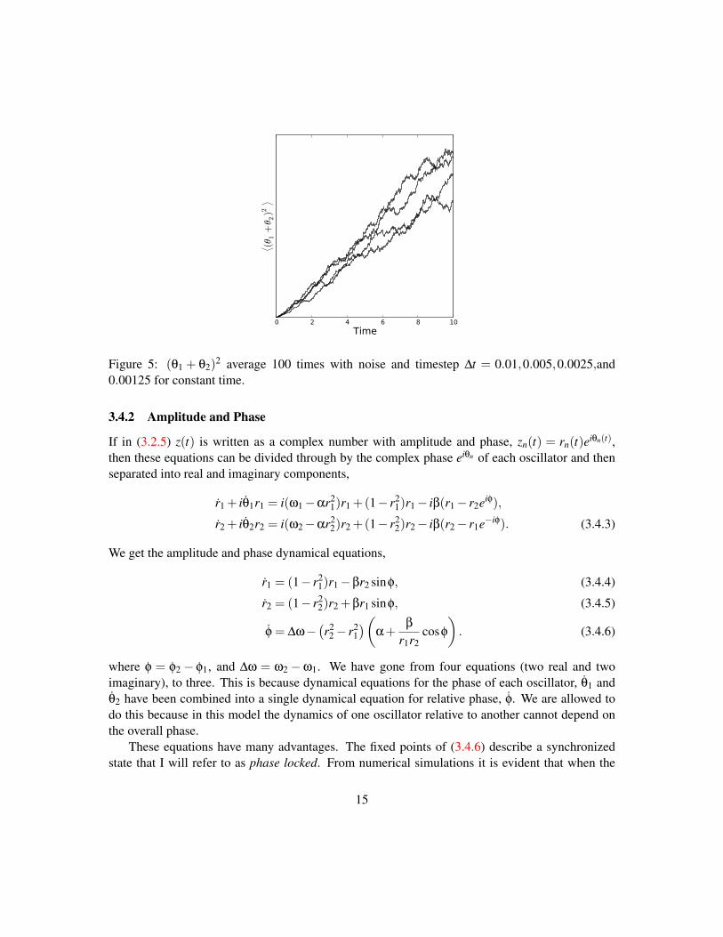
5 (θ1 +θ2)2 average 100 times with noise and timestep ∆t = 0.01,0.005,0.0025,and0.00125 for constant time. . . . . . . . . . . . . . . . . . . . . . . . . . . . . . . 15

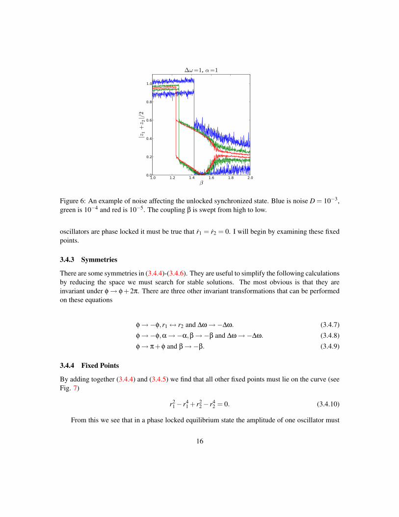
6 An example of noise affecting the unlocked synchronized state. Blue is noise D =10−3, green is 10−4 and red is 10−5. The coupling β is swept from high to low. . . 16

7 Curve of positive solutions to (3.4.10). The solid curve is r1 = s1,r2 = s2 (3.4.11),and the dotted curve is r1 = u1,r2 = u2 (3.4.12) . . . . . . . . . . . . . . . . . . . 17

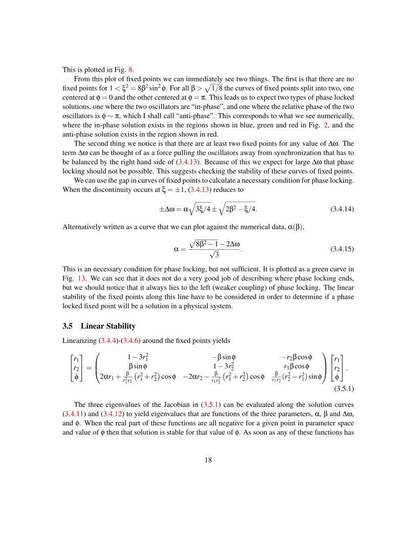
8 Plots of ∆ω as a function of φ for a constant value of α = 1 and β values of 0.3,0.36, 0.4 and 1. Every point along these curves are fixed points for a given set ofparameters ∆ω,α,β. The red curves correspond to (3.4.13) evaluated with r1 = u1and r2 = u2 (3.4.12), and the blue line corresponds to evaluations with r1 = s1 andr2 = s2 (3.4.11). The dotted portions of the curves represents fixed points which areunstable. The stability was calculated by evaluating the Jacobian (3.5.1) for eachpoint φ along the curve r1 = s1,r2 = s2 or r1 = u1,r2 = u2. We see that the set offixed points where r1 = u1,r2 = u2 is always unstable. We also see that the in-phaselocked solution is stable for small enough ∆ω, and that the anti-phase solution hasa minimum β for which it is stable. . . . . . . . . . . . . . . . . . . . . . . . . . . 19

4

9 Eigenvalues of (3.5.1) as a function of φ, evaluated at r1 = u1 and r2 = u2. Noticethat at least one of the eigenvalues always has a positive real component for allvalues of φ. The solid curves are the real components of the eigenvalues, and thedotted curves are the imaginary components. . . . . . . . . . . . . . . . . . . . . . 20

10 Eigenvalues of (3.5.1) as a function of φ, evaluated at r1 = s1 and r2 = s2. Thesolid curves are the real components of the eigenvalues, and the dotted curves arethe imaginary components. . . . . . . . . . . . . . . . . . . . . . . . . . . . . . . 20

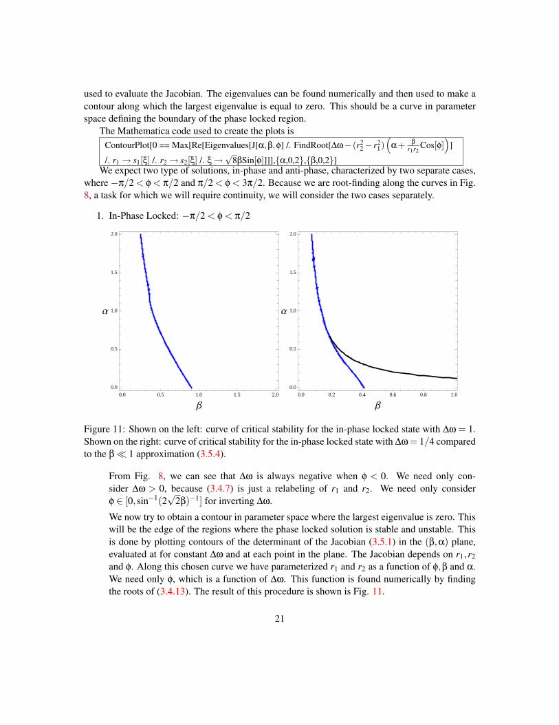
11 Shown on the left: curve of critical stability for the in-phase locked state with∆ω = 1. Shown on the right: curve of critical stability for the in-phase locked statewith ∆ω = 1/4 compared to the β 1 approximation (3.5.4). . . . . . . . . . . . 21

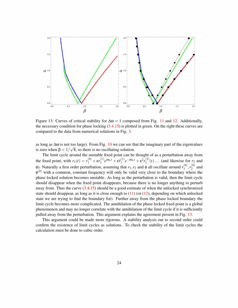
12 Curve of critical stability for anti-phase locked state with ∆ω = 1. . . . . . . . . . 2313 Curves of critical stability for ∆ω = 1 composed from Fig. 11 and 12. Additionally,

the necessary condition for phase locking (3.4.15) is plotted in green. On the rightthese curves are compared to the data from numerical solutions in Fig. 3. . . . . . 24

14 Left: Fourier transform of z1 and z2 at ∆ω = 1,α = 1,β = 1.62, when the oscillatorsare in the unlocked synchronized state. Right: r1,r2 and φ. . . . . . . . . . . . . . 25

5

1 Introduction

Numerous physical systems can be modeled by interacting oscillators [6]. An exciting quality ofsuch systems is their ability to oscillate collectively at a common frequency or phase even whenthe individual oscillators have different intrinsic frequencies or initial phases. This phenomenon isknown as synchronization. Small groups of oscillators are directly applicable to synchronizing sys-tems, such as lasers that are coupled to increase power output [4], and nanomechanical oscillators,where synchronization to a common frequency can eliminate the inevitable frequency differencesarising from imperfections in fabrication [2]. Understanding small numbers of coupled oscillatorscan be useful in the development of “renormalization group” methods to analyze very large systems(such as the synchronized flashing of fireflies [1]).

The general solution to a system of nonlinear oscillators can be very complicated. However,specific solutions can be obtained by taking the limit as the number of oscillators gets either verylarge or very small and then simplifying various aspects, such as assuming that only phase mattersor assuming some symmetry, such as a coupling between oscillators that is all-to-all [5]. Previouswork in this field has focused on the continuum limit of a very large number of oscillators and thelimit of very small number of oscillators. In this project I investigate a discrete systems of twononlinear oscillators.

This paper is organized as follows. After an introduction the devices motivating the body ofwork presented in this paper, I will derive the terms used in the equations of motion of the modelfrom the physical properties of the device. I then explore the behavior of the equations by findingnumerical solutions using explicit iterative methods. The observed behavior is used to developan intuition then used to approach the model analytically, using methods typical of dynamicalequations.

2 Devices

Devices are currently being designed, fabricated and developed by Matt Matheny in MichaelRoukes’s group at Caltech. There are two different devices currently being worked on.

The first type of device is single beam on a chip made of a thin piezoelectric material sand-wiched between a p-doped and n-doped layer of GaAs. The piezoelectric material is off-center, sowhen a voltage is applied to the piezoelectric layer causing it to expand, it strains the beam andcausing it to buckle. The beam is placed on one end of a cavity and probed optically with a laser.As the beam buckles, this changes the cavity length and modulates the power in the cavity, whichis then detected by shining the laser on a photodiode. The signal from the photodiode is then am-plified and phase-shifted so that is satisfies the Barkhausen criterion for oscillation, and then usedto drive the piezoelectric, completing the loop.

The piezoelectric beam is a very clean system. It can be probed optically and achieves a strongsignal and a very good signal to noise ratio. The primary disadvantage of this system is thatmultiplexing is not possible. Multiple oscillating piezoelectric beams on a single chip cannot be

6

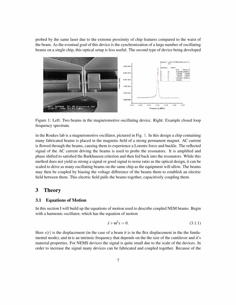
probed by the same laser due to the extreme proximity of chip features compared to the waist ofthe beam. As the eventual goal of this device is the synchronization of a large number of oscillatingbeams on a single chip, this optical setup is less useful. The second type of device being developed

Figure 1: Left: Two beams in the magnetomotive oscillating device. Right: Example closed loopfrequency spectrum.

in the Roukes lab is a magnetomotive oscillator, pictured in Fig. 1. In this design a chip containingmany fabricated beams is placed in the magnetic field of a strong permanent magnet. AC currentis flowed through the beams, causing them to experience a Lorentz force and buckle. The reflectedsignal of the AC current driving the beams is used to probe the resonators. It is amplified andphase shifted to satisfied the Barkhausen criterion and then fed back into the resonators. While thismethod does not yield as strong a signal or good signal to noise ratio as the optical design, it can bescaled to drive as many oscillating beams on the same chip as the equipment will allow. The beamsmay then be coupled by biasing the voltage difference of the beams them to establish an electricfield between them. This electric field pulls the beams together, capacitively coupling them.

3 Theory

3.1 Equations of Motion

In this section I will build up the equations of motion used to describe coupled NEM beams. Beginwith a harmonic oscillator, which has the equation of motion

x+ω2x = 0. (3.1.1)

Here x(t) is the displacement (in the case of a beam it is in the flex displacement in the the funda-mental mode), and ω is an intrinsic frequency that depends on the the size of the cantilever and it’smaterial properties. For NEMS devices the signal is quite small due to the scale of the devices. Inorder to increase the signal many devices can be fabricated and coupled together. Because of the

7

dependence of intrinsic frequency on the size and makeup of each device, intrinsic frequency canvary greatly during actual fabrication of multiple oscillators. It is then important that the devicesbe synchronized so that they oscillate at a single frequency. I will consider the case of two devicesreactively coupled. This is done by giving one beam some bias voltage and holding the potentialof the other beam to ground. This establishes an electric field between the two beams which pullsthem together. Including the coupling term and writing equations for two coupled oscillators, theequations of motion are now

x1 +ω21x1−B(x1− x2) = 0,

x2 +ω22x2−B(x2− x1) = 0, (3.1.2)

where B is proportional to the strength of the coupling force, and ω1 and ω2 are the intrinsicfrequencies of the separate oscillators. Because the coupling term is proportional to displacementit is invariant under time reversal, and so we call it reactive.

For a spring that obeys Hook’s law, stretching or compressing spring with spring constant kand rest length l to new length l′ results in a restoring force of magnitude F = k|l− l′|. As a toymodel for a beam, consider two springs of rest length l, one with endpoints at (−l,0) and (0,0)and the other with endpoints at (l,0) and (0,0). If the springs are connected at (0,0) and then thisconnected point is displaced to (0,y), then the restoring force will be directed toward (0,0) andhave magnitude

F = 2kl

(√y2

l2 +1−1

)y

l√

y2

l2 +1

yl≈ k

ly3. (3.1.3)

This restoring force that has a cubic dependence on displacement which I will refer to as a Duffingterm. It is a characteristic feature of the Duffing equation, which describes a spring that stiffens asit is stretched,

x1 +ω21x1−B(x1− x2)+ax3

1 = 0,

x2 +ω22x2−B(x2− x1)+ax3

2 = 0. (3.1.4)

We will see in the next section that this term causes the intrinsic frequency of the beam to shiftas the oscillations grow in amplitude. With the addition of this term the differential equations ofmotion are nonlinear. Finally, a Van der Pol term is added,

x1 +ω21x1−B(x1− x2)+ax3

1 +ν(x21−1)x1 = 0,

x2 +ω22x2−B(x2− x1)+ax3

2 +ν(x22−1)x2 = 0. (3.1.5)

This term that drives the system towards a limit cycle with xn near unity. It is comprised of negativelinear damping, which models the energy injected into the system through a feedback loop, andpositive nonlinear damping, which models the loses due to friction and other sources.

8

3.2 Perturbation Theory

Above I assume that a and ν are constant for all oscillators, and that the intrinsic frequency ωn

would be the feature that varied the most across oscillators. This assumption is valid because in thesystem we are trying to model a and ν are observed to be small, thus any variation is dominated bythe variations in ωn.

In this section we will try to solve (3.1.5) by perturbing away from a harmonic oscillator andthen eliminating what are known as “secular” terms. The objective will be to remove the fast,“nearly harmonic” oscillations and focus on the slower nonlinear effects.

If the frequency is expressed as deviations around some center frequency ω2n = ω2(1 + δn),

then the center frequency ω may be removed by choosing a new timescale t → t/ω, and scalingthe parameters a→ aω2 , ν→ νω and B→ Bω2. It now is convenient to only write equations fora single fiducial oscillator we are interested in, which I will call x(t), and refer to the oscillator itis coupled to as x(t). I will use the subscripts to refer to a term in a series expansion of x(t). Theequation of motion now is written

x+(1+δ)x−B(x− x)+ax3 +ν(x2−1)x = 0. (3.2.1)

If all the parameters δ,a,ν and B are much smaller than unity we can perturb away from the har-monic oscillator solution with a two timescale approximation. These parameters can be expressedas being small perturbations by scaling them by a small factor ε 1,

x+(1+ εδ)x− εB(x− x)+ εax3 + εν(x2−1)x = 0. (3.2.2)

For ε = 0 this is a simple harmonic oscillator with frequency 1. The proposed solution to thisequation is an expansion of x(t) in orders of ε. We will only carry out the calculation to first orderin ε. Additionally, we will modulate the harmonic oscillator solution over a much slower time scalewith a complex amplitude A(T ), where T = εt, so that x(t) = A(T )eit + A(T )e−it . The complexconjugate is used to ensure that x(t) is real, as it is a measurable physical quantity. We will treat T asan independent variable from t and express A(εt) = ∂A/∂t = (∂A/∂T )(∂T/∂t) = ε∂A/∂T = εA′(T ).The derivatives of the proposed solution are,

x(t) = iA(T )eit − iA(T )e−it + ε(A′(T )eit + A′(T )e−it)+ εx1(t)+O(ε2),

x(t) =−A(T )eit − A(T )e−it +2iε(A′(T )eit − A′(T )e−it)+ εx1(t)+O(ε2).

These are substituted into (3.2.2). We require that all orders of ε must vanish separately. Thezeroth order equation is that of the harmonic oscillator and is automatically satisfied by the e±it

term of x(t). The first order equation is

9

x1 + x1 +2i(A′eit − A′e−it)+δ(Aeit − Ae−it)−B(Aeit + Ae−it − Aeit + ¯Ae−it)

+a(A3e3it +3|A|2Aeit +3|A|2Ae−it A3e−3it)

+iν(A3e3it +(|A|2−1)Aeit − (|A|2−1)Ae−it − A3e−3it) = 0. (3.2.3)

We can identify this equation as the harmonic oscillator equation with periodic forcing terms.The e±it term is known as a secular1 term. This term is a resonant forcing and will cause theamplitude of the corrective term x1(t) to grow in time. In order for the stated perturbation theoryto be faithful to the original assumptions, x1(t) may not grow to be large, so the secular term mustbe eliminated. We use the free parameter introduced by the two timescale expansion to set thecoefficients of e±it to zero: The e±3it does not create a solution that grows in amplitude with time,so there is no need to remove it. Setting the coefficients of the secular term equal to zero, we have

2iA′+δA−B(A− A)+3a|A|2A+ iν(|A|2−1)A = 0. (3.2.4)

This is a first order dynamical equation. We end our perturbation theory here, as this providesthe rest of the information of the zeroth order term, and can be used to calculate the first ordercorrection. Define new variables z(νT/2) = A(T ), ω = δ/ν, α = −3a/ν, β = B/ν. I will alsoreturn to using z to mean a time derivative of z, now with respect to the rescaled time νT/2. Theequations for both oscillators written in their entirety are

z1 = i(ω1−α|z1|2)z1 +(1−|z1|2)z1− iβ(z1− z2),

z2 = i(ω2−α|z2|2)z2 +(1−|z2|2)z2− iβ(z2− z1). (3.2.5)

This is a first order system of dynamical equations, which is easy to solve for a given set ofz1(t),z2(t) using a Runge-Kutta method to iterate from z1(0),z2(0) with t/∆t intermediatesteps. Through this perturbation theory we have removed the fast time scale of the harmonicoscillator and left only the slower time scale nonlinear contribution. With the fast time dependenceremoved we are free to use larger time steps ∆t with the Runge-Kutta.

3.3 Numerical Simulation

I performed numerical implicit integration on (3.2.5) using a fourth order Runge Kutta iterativemethod (RK4) implemented in Python. With this as a base I constructed a library of functions to

1I had not previously seen the word “secular” used in this context. I had previously always thought it to refer tosomething of state or to mean“worldly”. It seems that this technical use of the world comes from astronomy, where itis used to mean slow changes in the motion of celestial objects. The etymology of the word is derived from the latinword saecularis meaning “of the age”. This was extended to long time phenomena, such as celestial mechanics, literallyoccurring over “ages”. In the context I am using it secular refers to the long timescale introduced to allow for the removalof secular terms from the perturbation theory.

10

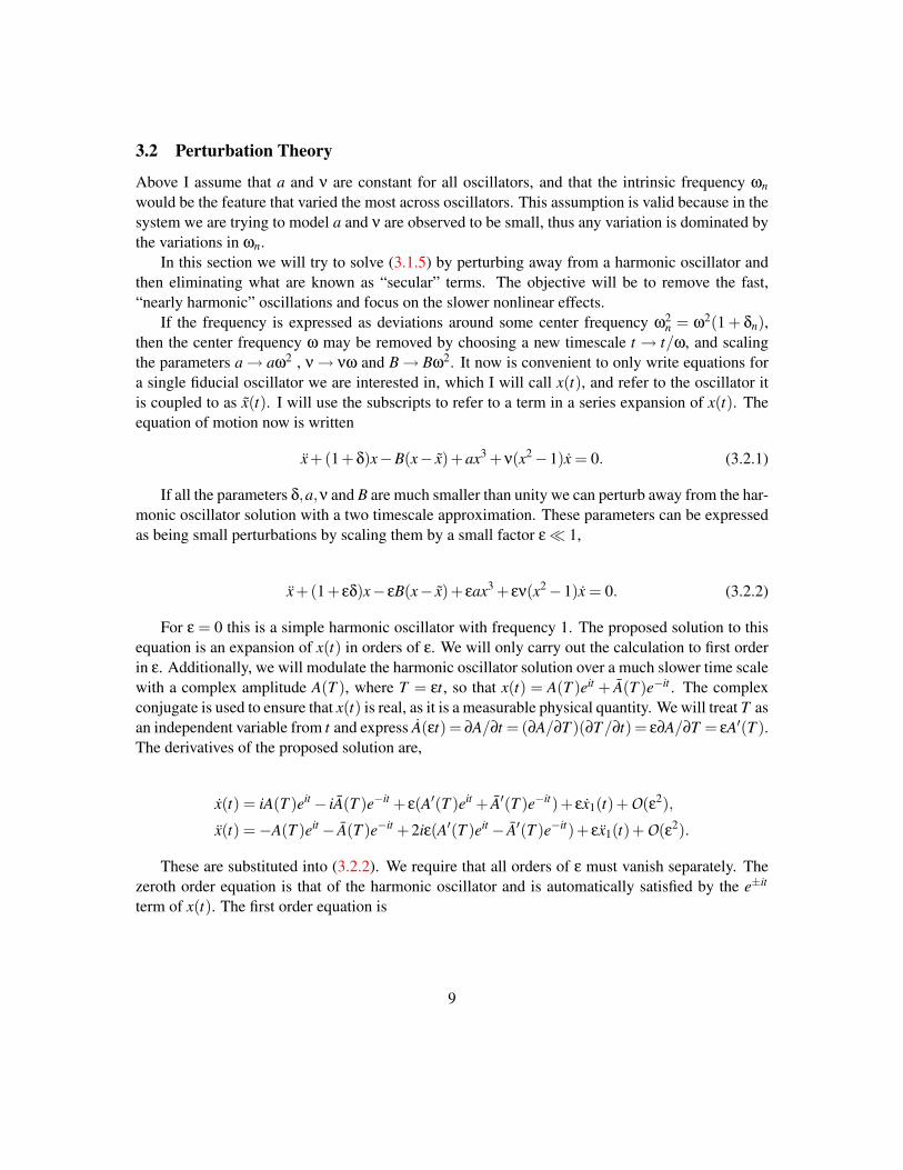
Figure 2: Survey of parameter space.

adiabatically sweep parameters (e.g. Fig. 3) and perform searches of parameter space (e.g. Fig.2). From performing many numerical calculations we can make several observations that will beessential to describing this system analytically. The first is that there are three classes of behavior:

Phase Locked Synchronization Both oscillators advance in time at a single common frequency.The relative phase between the oscillators is constant.

Unlocked Synchronization The relative phase between the two oscillators is not constant, butphase slips do not occur. The phase of one oscillator never advances more than 2π ahead ofthe other.

No Synchronization Each oscillator advances in time at it’s own frequency, affected by the otheroscillator a negligible amount. The relative phase between the oscillators will increase intime without bound.

11

The second is that for both the locked and unlocked synchronized state there are solutions wherethe phase difference φ of the two oscillators is very close to zero, which I will refer to as “in-phase”. There are also solutions where the relative phase φ is closer to π, which I will refer to as“anti-phase”.

How these three classes occupy parameter space can be seen in Fig. 2. At each (β,α) pairperform RK4 for 15 random initial conditions. The hope here is to explore the space of initialconditions so that at least one of the 15 points is in each of the different basins of attraction forthe different classes of behavior. Then the result of the RK is checked to determine what class ofbehavior occured. If none phase lock, color that point white (no synchronization). If all 15 phaselock with 0 < φ < π/2 the point is colored blue (a single phase locked state exists here). If all 15phase lock but for some π/2 < φ < π and and 0 < φ < π/2 for others the point is colored red (twophase locked states exist here). If some, but not all, of the 15 RK phase lock color then that pixelis colored green (both a phase locked and unlocked synchronized state exist here).

This search of parameter space can give us a good idea of what behavior we expect from theoscillators. We first see that exactly what we expect, that they synchronize for large values of thecoupling β, and that the nonlinearity α plays some role as well.

The goal in the later sections will be to calculate where the boundary of these regions will occur,and at the same time to understand what causes them. A more detailed view of the boundaries is inFig. 3. This figure shows very slow sweeps of parameter β, and where transitions occur for a given(β,α) which is plotted as a point on the left plot.

The effect of synchronization on the frequency spectrum of the oscillators is shown in Fig. 4.Here the intrinsic frequency ω0 of one is held fixed as the other ω1 is swept from−3 to 5. Betweenabout −1 and 3 the oscillators have phase locked and exhibit a single common frequency. At ω1outside this region the spectrum of each oscillator is more diverse as the frequencies of z1 and z2beat.

I also implemented a second order stochastic Runge Kutta (SRK2) in Python for numericalsimulations including white noise[3]. I’ve included a benchmark test of the noise I made to ensureit was a proper stochastic Runge Kutta method, Fig. 5. The sum of the absolute phase of the twooscillators experiences no forces, so in the presence of noise it should undergo a random walk. Theexpected value of a random walk is proportional to

√T , so

⟨(θ1 +θ2)2

⟩should increase linearly

in time. I approximate the expected value by averaging 100 SRK runs. This figure shows thatfor constant time and different number of iterative steps the noise stays constant, proving that thisimplementation of SRK is correct.

In Fig. 6 an example of the effect of noise on the solutions. This is a sweep of coupling strengthlike in Fig. 3, but as the amount of noise increases we can see that the jump from the anti-phaseunlocked state to the in-phase locked state occurs for stronger couplings.

12

æ

æ

æ

æ

æ

æ

æ

æ

æ

æ

à

à

à

à

à

à

à

ì

ì

ì

ì

ì

ì

ì

ò

ò

ò

ò0.0 0.5 1.0 1.5 2.0 Β0.0

0.5

1.0

1.5

2.0Α

Figure 3: Left: Boundary data obtained from slow sweeps of β for set α and ∆ω = 1. The bluecurve (circles) corresponds to the boundary of the in-phase locked solution. The red curve (squares)corresponds to the boundary of the anti-phase locked solution. The diamonds are the boundaryof the anti-phase unlocked solution, and the triangles are the boundary to the in phase lockedsynchronized state. The sweeps that generated this data are pictured on the right. Right: In theseβ is slowly swept from 2 to 0 for set α and ∆ω. Here the excursion of |z1 + z2|/2 is plotted. Whenthe oscillators are phase locked this should be a single line. When unlocked or not synchronizedthe excursion will increase, because the amplitudes and phases are changing in time. We can seethat there are two phase locked solutions, the in-phase solution where |z1 + z2|/2 is near 1, and theanti-phase solution, where |z1 +z2|/2 is near 0. As β is swept from 2 to 0 we see that the anti-phasesolution becomes unlocked (shaded red), and then jumps to the in-phase solution. Finally as β isswept lower the in-phase solution unlocks (blue) and synchronization is lost (grey).

1 c l a s s s t o c h a s t i c r u n g e k u t t a :2 def i n i t ( s e l f , da t a , f , t ime =0 , d t = 0 . 0 1 ) :3 s e l f . d a t a = a r r a y ( d a t a )4 s e l f . t ime = f l o a t ( t ime )5 s e l f . d t = f l o a t ( d t )6 s e l f . f = f7 s e l f .D = 08

9 def s t e p ( s e l f , d t , d a t a ) :10 ””” W i l l t a k e a s i n g l e SRK2 s t e p o f d t from p o i n t da ta ”””11 p s i = d o t ( s q r t (2∗ s e l f .D∗ d t ) , random . normal ( s i z e = ( 2 , l e n ( d a t a ) ) ) )12 k1 = s e l f . f ( s e l f . t ime , d a t a )13 k2 = s e l f . f ( s e l f . t ime +dt , d a t a + d t ∗k1+ p s i [ 0 ] + 1 j ∗ p s i [ 1 ] )14 re turn d a t a + ( d t / 2 ) ∗ ( k1+k2 )+ p s i [ 0 ] + 1 j ∗ p s i [ 1 ]

13

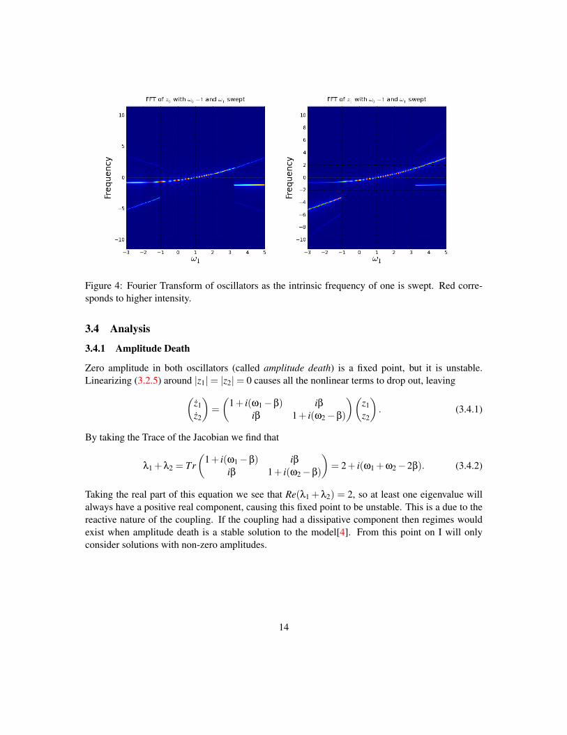
Figure 4: Fourier Transform of oscillators as the intrinsic frequency of one is swept. Red corre-sponds to higher intensity.

3.4 Analysis

3.4.1 Amplitude Death

Zero amplitude in both oscillators (called amplitude death) is a fixed point, but it is unstable.Linearizing (3.2.5) around |z1|= |z2|= 0 causes all the nonlinear terms to drop out, leaving(

z1z2

)=(

1+ i(ω1−β) iβiβ 1+ i(ω2−β)

)(z1z2

). (3.4.1)

By taking the Trace of the Jacobian we find that

λ1 +λ2 = Tr(

1+ i(ω1−β) iβiβ 1+ i(ω2−β)

)= 2+ i(ω1 +ω2−2β). (3.4.2)

Taking the real part of this equation we see that Re(λ1 + λ2) = 2, so at least one eigenvalue willalways have a positive real component, causing this fixed point to be unstable. This is a due to thereactive nature of the coupling. If the coupling had a dissipative component then regimes wouldexist when amplitude death is a stable solution to the model[4]. From this point on I will onlyconsider solutions with non-zero amplitudes.

14

0 2 4 6 8 10

Time

⟨ (θ1

+θ 2

)2⟩

Figure 5: (θ1 + θ2)2 average 100 times with noise and timestep ∆t = 0.01,0.005,0.0025,and0.00125 for constant time.

3.4.2 Amplitude and Phase

If in (3.2.5) z(t) is written as a complex number with amplitude and phase, zn(t) = rn(t)eiθn(t),then these equations can be divided through by the complex phase eiθn of each oscillator and thenseparated into real and imaginary components,

r1 + iθ1r1 = i(ω1−αr21)r1 +(1− r2

1)r1− iβ(r1− r2eiφ),

r2 + iθ2r2 = i(ω2−αr22)r2 +(1− r2

2)r2− iβ(r2− r1e−iφ). (3.4.3)

We get the amplitude and phase dynamical equations,

r1 = (1− r21)r1−βr2 sinφ, (3.4.4)

r2 = (1− r22)r2 +βr1 sinφ, (3.4.5)

φ = ∆ω−(r2

2− r21)(

α+β

r1r2cosφ

). (3.4.6)

where φ = φ2− φ1, and ∆ω = ω2−ω1. We have gone from four equations (two real and twoimaginary), to three. This is because dynamical equations for the phase of each oscillator, θ1 andθ2 have been combined into a single dynamical equation for relative phase, φ. We are allowed todo this because in this model the dynamics of one oscillator relative to another cannot depend onthe overall phase.

These equations have many advantages. The fixed points of (3.4.6) describe a synchronizedstate that I will refer to as phase locked. From numerical simulations it is evident that when the

15

1.0 1.2 1.4 1.6 1.8 2.0

β

0.0

0.2

0.4

0.6

0.8

1.0

|z1

+z 2|/

2

∆ω=1, α=1

Figure 6: An example of noise affecting the unlocked synchronized state. Blue is noise D = 10−3,green is 10−4 and red is 10−5. The coupling β is swept from high to low.

oscillators are phase locked it must be true that r1 = r2 = 0. I will begin by examining these fixedpoints.

3.4.3 Symmetries

There are some symmetries in (3.4.4)-(3.4.6). They are useful to simplify the following calculationsby reducing the space we must search for stable solutions. The most obvious is that they areinvariant under φ→ φ+2π. There are three other invariant transformations that can be performedon these equations

φ→−φ,r1↔ r2 and ∆ω→−∆ω. (3.4.7)

φ→−φ,α→−α,β→−β and ∆ω→−∆ω. (3.4.8)

φ→ π+φ and β→−β. (3.4.9)

3.4.4 Fixed Points

By adding together (3.4.4) and (3.4.5) we find that all other fixed points must lie on the curve (seeFig. 7)

r21− r4

1 + r22− r4

2 = 0. (3.4.10)

From this we see that in a phase locked equilibrium state the amplitude of one oscillator must

16

r 0.2 0.4 0.6 0.8 1.0 r1

0.2

0.4

0.6

0.8

1.0

r2

Figure 7: Curve of positive solutions to (3.4.10). The solid curve is r1 = s1,r2 = s2 (3.4.11), andthe dotted curve is r1 = u1,r2 = u2 (3.4.12)

be greater than one, and the other less than one. We can break this curve into two parts, by parame-terizing r1 and r2 with ξ2 = 8β2 sin2

φ. The two parts are r1 = s1,r2 = s2 and r1 = u1,r2 = u2,where u1,u2,s1,s2 are functions of parameter ξ and defined as

s1 =12

√3+√

1−ξ2− sign(ξ)√

2+ξ2−2√

1−ξ2,

s2 =12

√3+√

1−ξ2 + sign(ξ)√

2+ξ2−2√

1−ξ2, (3.4.11)

u1 =12

√3−√

1−ξ2− sign(ξ)√

2+ξ2 +2√

1−ξ2,

u2 =12

√3−√

1−ξ2 + sign(ξ)√

2+ξ2 +2√

1−ξ2. (3.4.12)

These are both plotted in (7). The solid curve is s1 and s2, and it sweeps from r1 =√

(3+√

3)/4,r2 =√(3−√

3)/4 at ξ = −1 to r1 =√

(3−√

3)/4,r2 =√

(3+√

3)/4 at ξ = 1, passing throughr1 = 1,r2 = 1 at ξ = 0. The dotted curve is u1 and u2 and has the same endpoints, although itjumps discontinuously from r1 = 1,r2 = 0 to r1 = 0,r2 = 1 at ξ = 0.

The fixed point of (3.4.6) is written as,

∆ω =(r2

2− r21)(

α+β

r1r2cosφ

)(3.4.13)

17

This is plotted in Fig. 8.From this plot of fixed points we can immediately see two things. The first is that there are no

fixed points for 1 < ξ2 = 8β2 sin2φ. For all β >

√1/8 the curves of fixed points split into two, one

centered at φ = 0 and the other centered at φ = π. This leads us to expect two types of phase lockedsolutions, one where the two oscillators are “in-phase”, and one where the relative phase of the twooscillators is φ∼ π, which I shall call “anti-phase”. This corresponds to what we see numerically,where the in-phase solution exists in the regions shown in blue, green and red in Fig. 2, and theanti-phase solution exists in the region shown in red.

The second thing we notice is that there are at least two fixed points for any value of ∆ω. Theterm ∆ω can be thought of as a force pulling the oscillators away from synchronization that has tobe balanced by the right hand side of (3.4.13). Because of this we expect for large ∆ω that phaselocking should not be possible. This suggests checking the stability of these curves of fixed points.

We can use the gap in curves of fixed points to calculate a necessary condition for phase locking.When the discontinuity occurs at ξ =±1, (3.4.13) reduces to

±∆ω = α

√3ξ/4±

√2β2−ξ/4. (3.4.14)

Alternatively written as a curve that we can plot against the numerical data, α(β),

α =

√8β2−1−2∆ω√

3. (3.4.15)

This is an necessary condition for phase locking, but not sufficient. It is plotted as a green curve inFig. 13. We can see that it does not do a very good job of describing where phase locking ends,but we should notice that it always lies to the left (weaker coupling) of phase locking. The linearstability of the fixed points along this line have to be considered in order to determine if a phaselocked fixed point will be a solution in a physical system.

3.5 Linear Stability

Linearizing (3.4.4)-(3.4.6) around the fixed points yieldsr1r2φ

=

1−3r21 −βsinφ −r2βcosφ

βsinφ 1−3r22 r1βcosφ

2αr1 + β

r21r2

(r2

1 + r22)

cosφ −2αr2− β

r1r22

(r2

1 + r22)

cosφβ

r1r2(r2

2− r21)sinφ

r1

r2φ

.

(3.5.1)

The three eigenvalues of the Jacobian in (3.5.1) can be evaluated along the solution curves(3.4.11) and (3.4.12) to yield eigenvalues that are functions of the three parameters, α, β and ∆ω,and φ. When the real part of these functions are all negative for a given point in parameter spaceand value of φ then that solution is stable for that value of φ. As soon as any of these functions has

18

-1 1 2 3 4 Φ

-3

-2

-1

1

2

3DΩ

Α = 1. Β = 0.3

-1 1 2 3 4 Φ

-3

-2

-1

1

2

3DΩ

Α = 1. Β = 0.36

-1 1 2 3 4 Φ

-3

-2

-1

1

2

3DΩ

Α = 1. Β = 0.4

-1 1 2 3 4 Φ

-3

-2

-1

1

2

3DΩ

Α = 1. Β = 1.

Figure 8: Plots of ∆ω as a function of φ for a constant value of α = 1 and β values of 0.3, 0.36,0.4 and 1. Every point along these curves are fixed points for a given set of parameters ∆ω,α,β.The red curves correspond to (3.4.13) evaluated with r1 = u1 and r2 = u2 (3.4.12), and the blueline corresponds to evaluations with r1 = s1 and r2 = s2 (3.4.11). The dotted portions of the curvesrepresents fixed points which are unstable. The stability was calculated by evaluating the Jacobian(3.5.1) for each point φ along the curve r1 = s1,r2 = s2 or r1 = u1,r2 = u2. We see that the setof fixed points where r1 = u1,r2 = u2 is always unstable. We also see that the in-phase lockedsolution is stable for small enough ∆ω, and that the anti-phase solution has a minimum β for whichit is stable.

19

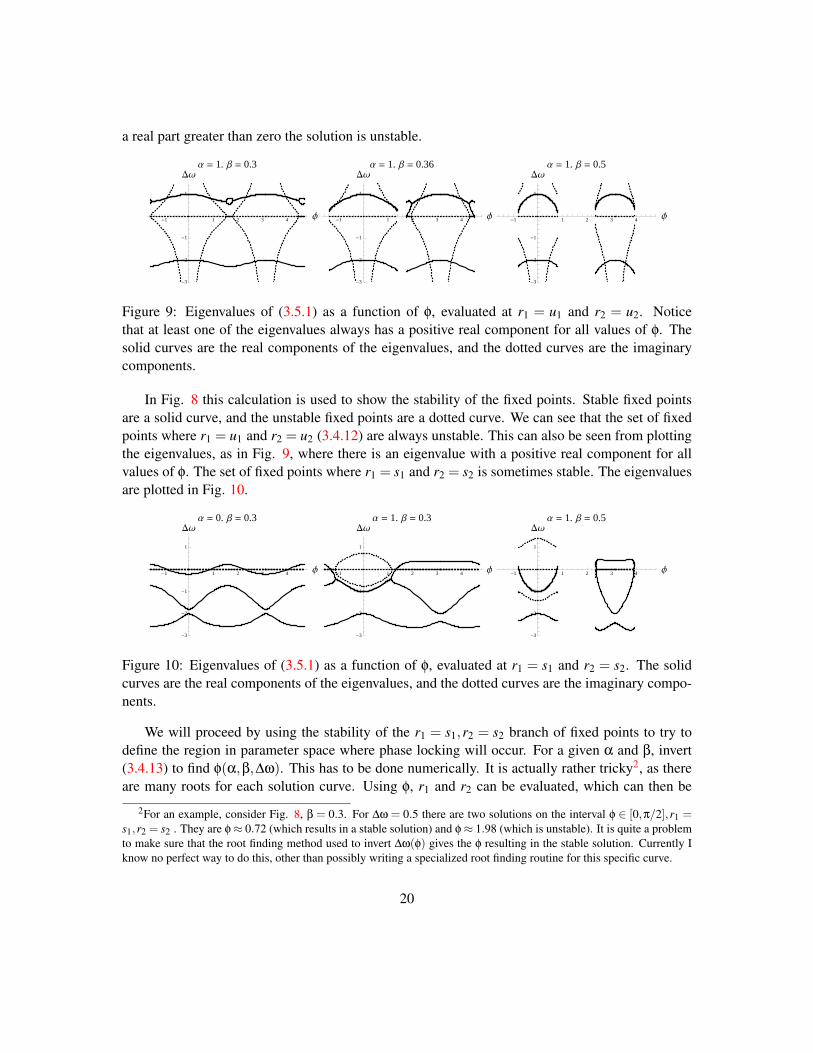
a real part greater than zero the solution is unstable.

-1 1 2 3 4 Φ

-3

-2

-1

1

DΩ

Α = 1. Β = 0.3

-1 1 2 3 4 Φ

-3

-2

-1

1

DΩ

Α = 1. Β = 0.36

-1 1 2 3 4 Φ

-3

-2

-1

1

DΩ

Α = 1. Β = 0.5

Figure 9: Eigenvalues of (3.5.1) as a function of φ, evaluated at r1 = u1 and r2 = u2. Noticethat at least one of the eigenvalues always has a positive real component for all values of φ. Thesolid curves are the real components of the eigenvalues, and the dotted curves are the imaginarycomponents.

In Fig. 8 this calculation is used to show the stability of the fixed points. Stable fixed pointsare a solid curve, and the unstable fixed points are a dotted curve. We can see that the set of fixedpoints where r1 = u1 and r2 = u2 (3.4.12) are always unstable. This can also be seen from plottingthe eigenvalues, as in Fig. 9, where there is an eigenvalue with a positive real component for allvalues of φ. The set of fixed points where r1 = s1 and r2 = s2 is sometimes stable. The eigenvaluesare plotted in Fig. 10.

-1 1 2 3 4 Φ

-3

-2

-1

1

DΩ

Α = 0. Β = 0.3

-1 1 2 3 4 Φ

-3

-2

-1

1

DΩ

Α = 1. Β = 0.3

-1 1 2 3 4 Φ

-3

-2

-1

1

DΩ

Α = 1. Β = 0.5

Figure 10: Eigenvalues of (3.5.1) as a function of φ, evaluated at r1 = s1 and r2 = s2. The solidcurves are the real components of the eigenvalues, and the dotted curves are the imaginary compo-nents.

We will proceed by using the stability of the r1 = s1,r2 = s2 branch of fixed points to try todefine the region in parameter space where phase locking will occur. For a given α and β, invert(3.4.13) to find φ(α,β,∆ω). This has to be done numerically. It is actually rather tricky2, as thereare many roots for each solution curve. Using φ, r1 and r2 can be evaluated, which can then be

2For an example, consider Fig. 8, β = 0.3. For ∆ω = 0.5 there are two solutions on the interval φ ∈ [0,π/2],r1 =s1,r2 = s2 . They are φ≈ 0.72 (which results in a stable solution) and φ≈ 1.98 (which is unstable). It is quite a problemto make sure that the root finding method used to invert ∆ω(φ) gives the φ resulting in the stable solution. Currently Iknow no perfect way to do this, other than possibly writing a specialized root finding routine for this specific curve.

20

used to evaluate the Jacobian. The eigenvalues can be found numerically and then used to make acontour along which the largest eigenvalue is equal to zero. This should be a curve in parameterspace defining the boundary of the phase locked region.

The Mathematica code used to create the plots isContourPlot[0 == Max[Re[Eigenvalues[J[α,β,φ] /. FindRoot[∆ω− (r2

2− r21)(

α+ β

r1r2Cos[φ]

)]

/. r1→ s1[ξ] /. r2→ s2[ξ] /. ξ→√

8βSin[φ]]]],α,0,2,β,0,2]We expect two type of solutions, in-phase and anti-phase, characterized by two separate cases,

where −π/2 < φ < π/2 and π/2 < φ < 3π/2. Because we are root-finding along the curves in Fig.8, a task for which we will require continuity, we will consider the two cases separately.

1. In-Phase Locked: −π/2 < φ < π/2

0.0 0.5 1.0 1.5 2.0

0.0

0.5

1.0

1.5

2.0

Β

Α

0.0 0.2 0.4 0.6 0.8 1.0

0.0

0.5

1.0

1.5

2.0

Β

Α

Figure 11: Shown on the left: curve of critical stability for the in-phase locked state with ∆ω = 1.Shown on the right: curve of critical stability for the in-phase locked state with ∆ω = 1/4 comparedto the β 1 approximation (3.5.4).

From Fig. 8, we can see that ∆ω is always negative when φ < 0. We need only con-sider ∆ω > 0, because (3.4.7) is just a relabeling of r1 and r2. We need only considerφ ∈ [0,sin−1(2

√2β)−1] for inverting ∆ω.

We now try to obtain a contour in parameter space where the largest eigenvalue is zero. Thiswill be the edge of the regions where the phase locked solution is stable and unstable. Thisis done by plotting contours of the determinant of the Jacobian (3.5.1) in the (β,α) plane,evaluated at for constant ∆ω and at each point in the plane. The Jacobian depends on r1,r2and φ. Along this chosen curve we have parameterized r1 and r2 as a function of φ,β and α.We need only φ, which is a function of ∆ω. This function is found numerically by findingthe roots of (3.4.13). The result of this procedure is shown is Fig. 11.

21

If we linearize the curve (3.4.10) near ξ = 0, we can approximate r1 and r2 as r1 = 1+δ andr2 = 1− δ, where δ 1. This is motivated by Fig. 7, where the slope of the curve aroundr1 = 1,r2 = 1 is −1. Plugging these into (3.4.4) and (3.4.5) and only keeping terms out tofirst order in δ we get

2δ+βsinφ =±δβsinφ. (3.5.2)

If we assume that β 1 then we find that δ = −12 βsinφ. Plugging this into (3.4.6) and

keeping terms out to first order in δ we find

∆ω =−4(α+βcosφ)δ = 2(α+βcosφ)βsinφ. (3.5.3)

The response to ∆ω is maximized at φ = π/2. For ∆ω beyond that there is no φ large enoughto balance the frequency difference and allow for synchronization. Thus the boundary be-tween phase locking and unlocked should occur at φ = 2π. This gives a guess that is goodfor β 1,

∆ω = 2αβ. (3.5.4)

Plotting this next to the phase locking boundary calculated from the linear stability of fixedpoints should yield good agreement for small β (less than about 0.2), see in Fig. 11.

2. Anti-Phase Locked: π/2 < φ < 3π/2

As in the previous case, ∆ω is only positive in one region for φ, when φ > π/2. Thus weneed only consider φ ∈ [π− sin−1(2

√2β)−1,π] and φ ∈ [π,π+ sin−1(2

√2β)−1]. The results

of the rootfinding are shown in Fig. 12.

3.6 Putting it all together

To characterize this system, we need to combine Fig. 11,12 into one picture that will tell us forwhat regions of parameter space different phase locked solutions will be stable or unstable. Byplotting these curves we construct a picture of the stability of all the solutions , shown in Fig. 13.In this figure we can see the two types phase locked states that exist, plotted in blue for 0 < φ < π/2and red for π/2 < φ < π. The agreement with the data from Runge-Kutta is very good.

Additionally we can see that curve defining the boundary for existence of phase-locking [(3.4.15)shown in green] has good agreement with the points where the unlocked, but still synchronized,solution ceases to exist. Why this occurs is explained in the next section.

22

0.0 0.5 1.0 1.5 2.0

0.0

0.5

1.0

1.5

2.0

Β

Α

Figure 12: Curve of critical stability for anti-phase locked state with ∆ω = 1.

3.7 Unlocked Synchronization

The fact that the unlocked synchronized states lie on the edge of the phase locked states in parame-ters space is a big hint as to their origin. Phase locking can no longer occur when the phase lockedfixed point becomes unstable. However, the phase locked solution still exists. I propose that whenthe the solution becomes unstable, nearby there is a stable limit cycle around the fixed point. Theexistence of such a limit cycle could be checked by extending the stability analysis to quadraticorder. Alternatively, we can first check numerically. We do indeed see that the unlocked synchro-nized states are stable limit cycles around the now unstable phase locked fixed points. An exampleis shown in Fig. 14. This is for β = 1.62, and the fixed point becomes unstable at roughly β = 1.63.At β = 1.62 the eigenvalue in the r1 and r2 direction have of a positive real component, and they areis λ± = 0.0113±2.908i. We expect the oscillation frequency of the limit cycle to be the imaginarypart of the eigenvalue, ωlc = 2.908, and this is what we see. The discrete Fourier transform is thatof the synchronized frequency of both oscillators (θ1 = θ2 = 4.743), beating against the frequencyof the limit cycle, yielding peaks in the Fourier transform at increments of 2.908 away from thecentral peak. By looking at the time evolution of r1,r2 and φ we see that they are essentially si-nusoids with the limit cycle frequency. We expect r1 and r2 to oscillate at ωlc, as those are thedirections with the imaginary component of the eigenvalue. The reason φ also oscillates at thisfrequency is that to stay a solution φ must adjust itself to follow r1 and r2. Since there is only onefrequency present φ must adjust itself at that frequency.

This same reasoning also explains the in-phase unlocked state. However, in this case, (3.4.15)stops at β = 1/

√8. For β < 1

√8 there is always a solution to (3.4.13) for a given value of φ (and

23

0.0 0.5 1.0 1.5 2.0

0.0

0.5

1.0

1.5

2.0

Β

Α

æ

æ

æ

æ

æ

æ

æ

æ

æ

æ

à

à

à

à

à

à

à

ì

ì

ì

ì

ì

ì

ì

ò

ò

ò

ò

0.0 0.5 1.0 1.5 2.0

0.0

0.5

1.0

1.5

2.0

Β

Α

Figure 13: Curves of critical stability for ∆ω = 1 composed from Fig. 11 and 12. Additionally,the necessary condition for phase locking (3.4.15) is plotted in green. On the right these curves arecompared to the data from numerical solutions in Fig. 3.

as long as ∆ω is not too large). From Fig. 10 we can see that the imaginary part of the eigenvaluesis zero when β < 1/

√8, so there is no oscillating solution.

The limit cycle around the unstable fixed point can be thought of as a perturbation away fromthe fixed point, with r1(t) = r(0)

1 + εr(1)1 eiωlct + εr(1)

1 e−iωlct + ε2r(2)1 (t) . . . (and likewise for r2 and

φ). Naturally a first order perturbation, assuming that r1,r2 and φ all oscillate around r(0)1 ,r(0)

2 andφ(0) with a common, constant frequency will only be valid very close to the boundary where thephase locked solution becomes unstable. As long as the perturbation is valid, then the limit cycleshould disappear when the fixed point disappears, because there is no longer anything to perturbaway from. Thus the curve (3.4.15) should be a good estimate of when the unlocked synchronizedstate should disappear, as long as it is close enough to (11) (or (12), depending on which unlockedstate we are trying to find the boundary for). Further away from the phase locked boundary thelimit cycle becomes more complicated. The annihilation of the phase locked fixed point is a globalphenomenon and may no longer correlate with the annihilation of the limit cycle if it is sufficientlypulled away from the perturbation. This argument explains the agreement present in Fig. 13.

This argument could be made more rigorous. A stability analysis out to second order couldconfirm the existence of limit cycles as solutions. To check the stability of the limit cycles thecalculation must be done to cubic order.

24

10 8 6 4 2 0 2

Frequency

10-3

10-2

10-1

100In

tensi

ty (

arb

)

Figure 14: Left: Fourier transform of z1 and z2 at ∆ω = 1,α = 1,β = 1.62, when the oscillators arein the unlocked synchronized state. Right: r1,r2 and φ.

4 Conclusions

In this thesis we have successfully characterized the behavior of our model. We fully explored theobserved behavior and classified the solutions into two synchronized states, an the in-phase andanti-phase solutions. These solutions exist as phase locked synchronized states for large couplingstrengths, and as unlocked synchronized states for smaller couplings before coming completelyunlocked. I’ve also developed the numerical tools necessary to run simulations of the oscillatorswith noise.

The very first thing to be done in followup is to wait with anticipation for the multiplexeddevice to be built and then compare how well its physical behavior matches what we expect basedon our calculations. Once this is finished there will surely be a lot of work still to be done on thetwo oscillator device and model.

The long term goal for these devices seems to be building as many beams on a chip as possibleand then synchronizing or driving them in exotic ways to do useful things. The next logical stepwould be to extend this work to describe a one dimensional array of oscillators coupled to theirnearest neighbors. The two oscillator result can be incorporated into a Renormalisation Grouptechnique and then applied to a large nearest neighbor coupled array.

25

5 Acknowledgements

First, my mentor and advisor, Mike Cross. He is entitled to 10% of the profits. Thanks to MattMatheny for building the actually oscillators this theory applies to and for providing all of thewonderful device pictures (1). He also took the time to show me his devices and explain everythingabout them to me, and for that I am indebted to him.

This project will hopefully end with this thesis, but it began as a Caltech SURF project. Inaddition to Mike Cross I was mentored by Mason Porter, who always demanded near perfectionbut less often received it from me. Additionally, Jeff Rogers and Ron Lifshitz were great to talk toabout my project. I also want to thank the Caltech SURF Office and Program, as well as Boeingfor funding. I hope that someday they get their theory of the airplane.

26

References

[1] J. Buck and E. Buck. Synchronous fireflies. Scientific American, 1974.

[2] Michael C. Cross, Jeffrey L. Rogers, Ron Lifshitz, and Alex Zumdieck. Synchronization byreactive coupling and nonlinear frequency pulling. Physical Review E, 73(036205), 2006.

[3] Rebecca L. Honeycutt. Stochastic runge-kutta algorithms. i. white noise. Phys. Rev. A, 45,1992.

[4] Jeffrey L. Rogers. Analysis of three coupled limit-cycle oscillators. Preprint, January 2007.

[5] Steven Strogatz. From Kuramoto to Crawford: Exploring the onset of synchronization inpopulations of coupled oscillators. Physica D, 143:1–20, 2000.

[6] Steven Strogatz. Sync: The Emerging Science of Spontaneous Order. Hyperion, 2003.

27