231


Theory of Adaptive Fiber Composites

SOLID MECHANICS AND ITS APPLICATIONSVolume 161
Series Editor: G.M.L. GLADWELLDepartment of Civil EngineeringUniversity of WaterlooWaterloo, Ontario, Canada N2L 3GI
Aims and Scope of the Series
The fundamental questions arising in mechanics are: Why?, How?, and How much?The aim of this series is to provide lucid accounts written by authoritative researchersgiving vision and insight in answering these questions on the subject of mechanics as itrelates to solids.
The scope of the series covers the entire spectrum of solid mechanics. Thus it includesthe foundation of mechanics; variational formulations; computational mechanics; statics,kinematics and dynamics of rigid and elastic bodies: vibrations of solids and structures;dynamical systems and chaos; the theories of elasticity, plasticity and viscoelasticity;composite materials; rods, beams, shells and membranes; structural control and stability;soils, rocks and geomechanics; fracture; tribology; experimental mechanics; biomechan-ics and machine design.
The median level of presentation is the first year graduate student. Some texts are mono-graphs defining the current state of the field; others are accessible to final year under-graduates; but essentially the emphasis is on readability and clarity.
For other titles published in this series, go towww.springer.com/series/6557

Tobias H. Brockmann
Theory of Adaptive FiberComposites
From Piezoelectric Material Behaviorto Dynamics of Rotating Structures

T.H. BrockmannDonauwö[email protected]
Approved Dissertation – Helmut-Schmidt-Universität, Hamburg, Germany
ISSN 0925-0042ISBN 978-90-481-2434-3 e-ISBN 978-90-481-2435-0DOI 10.1007/978-90-481-2435-0Springer Dordrecht Heidelberg London New York
Library of Congress Control Number: 2009925999
c©Springer Science+Business Media B.V. 2009No part of this work may be reproduced, stored in a retrieval system, or transmitted in any form or byany means, electronic, mechanical, photocopying, microfilming, recording or otherwise, without writtenpermission from the Publisher, with the exception of any material supplied specifically for the purpose ofbeing entered and executed on a computer system, for exclusive use by the purchaser of the work.
Printed on acid-free paper
Springer is part of Springer Science+Business Media (www.springer.com)
Contents
1 Introduction . . . . . . . . . . . . . . . . . . . . . . . . . . . . . . . . . . . . . . . . . . . . . . . 11.1 Adaptive Structural Systems . . . . . . . . . . . . . . . . . . . . . . . . . . . . . . 11.2 Objective and Scope . . . . . . . . . . . . . . . . . . . . . . . . . . . . . . . . . . . . . 21.3 Outline and Overview . . . . . . . . . . . . . . . . . . . . . . . . . . . . . . . . . . . . 3
2 Helicopter Applications . . . . . . . . . . . . . . . . . . . . . . . . . . . . . . . . . . . . 52.1 Noise and Vibration . . . . . . . . . . . . . . . . . . . . . . . . . . . . . . . . . . . . . 5
2.1.1 Generation . . . . . . . . . . . . . . . . . . . . . . . . . . . . . . . . . . . . . . . 52.1.2 Areas of Relevance . . . . . . . . . . . . . . . . . . . . . . . . . . . . . . . . 7
2.2 Main Rotor . . . . . . . . . . . . . . . . . . . . . . . . . . . . . . . . . . . . . . . . . . . . . 82.2.1 Rotational Sources . . . . . . . . . . . . . . . . . . . . . . . . . . . . . . . . 82.2.2 Impulsive Sources . . . . . . . . . . . . . . . . . . . . . . . . . . . . . . . . . 92.2.3 Broadband Sources . . . . . . . . . . . . . . . . . . . . . . . . . . . . . . . . 10
2.3 Passive Concepts . . . . . . . . . . . . . . . . . . . . . . . . . . . . . . . . . . . . . . . . 102.3.1 External Devices . . . . . . . . . . . . . . . . . . . . . . . . . . . . . . . . . . 102.3.2 Aeroelastic Conformability . . . . . . . . . . . . . . . . . . . . . . . . . 11
2.4 Active and Adaptive Concepts . . . . . . . . . . . . . . . . . . . . . . . . . . . . 132.4.1 Pitch Control at the Blade Root . . . . . . . . . . . . . . . . . . . . 132.4.2 Discrete Flap Actuation . . . . . . . . . . . . . . . . . . . . . . . . . . . . 142.4.3 Integral Blade Actuation . . . . . . . . . . . . . . . . . . . . . . . . . . . 14
2.5 Adaptive Beam Aspects . . . . . . . . . . . . . . . . . . . . . . . . . . . . . . . . . . 152.5.1 Beam Actuation Concepts . . . . . . . . . . . . . . . . . . . . . . . . . . 162.5.2 Adaptive System Concepts . . . . . . . . . . . . . . . . . . . . . . . . . 172.5.3 Development Status . . . . . . . . . . . . . . . . . . . . . . . . . . . . . . . 17
3 Fundamental Considerations . . . . . . . . . . . . . . . . . . . . . . . . . . . . . . . 193.1 Mathematical Preliminaries . . . . . . . . . . . . . . . . . . . . . . . . . . . . . . . 19
3.1.1 Euclidean Vectors . . . . . . . . . . . . . . . . . . . . . . . . . . . . . . . . . 193.1.2 Tensor Representation . . . . . . . . . . . . . . . . . . . . . . . . . . . . . 203.1.3 Matrix Representation . . . . . . . . . . . . . . . . . . . . . . . . . . . . . 21

vi Contents
3.2 Deformable Structures–Mechanical Fields . . . . . . . . . . . . . . . . . . . 223.2.1 Loads . . . . . . . . . . . . . . . . . . . . . . . . . . . . . . . . . . . . . . . . . . . . 233.2.2 Stresses . . . . . . . . . . . . . . . . . . . . . . . . . . . . . . . . . . . . . . . . . . 233.2.3 Mechanical Equilibrium . . . . . . . . . . . . . . . . . . . . . . . . . . . . 243.2.4 Strains . . . . . . . . . . . . . . . . . . . . . . . . . . . . . . . . . . . . . . . . . . . 253.2.5 Transformations . . . . . . . . . . . . . . . . . . . . . . . . . . . . . . . . . . . 26
3.3 Dielectric Domains–Electrostatic Fields . . . . . . . . . . . . . . . . . . . . 283.3.1 Electric Charge . . . . . . . . . . . . . . . . . . . . . . . . . . . . . . . . . . . 293.3.2 Electric Flux Density . . . . . . . . . . . . . . . . . . . . . . . . . . . . . . 293.3.3 Electrostatic Equilibrium . . . . . . . . . . . . . . . . . . . . . . . . . . . 293.3.4 Electric Field Strengths . . . . . . . . . . . . . . . . . . . . . . . . . . . . 30
3.4 Principle of Virtual Work . . . . . . . . . . . . . . . . . . . . . . . . . . . . . . . . . 313.4.1 General Principle of Virtual Work . . . . . . . . . . . . . . . . . . . 313.4.2 Principle of Virtual Displacements . . . . . . . . . . . . . . . . . . . 323.4.3 Principle of Virtual Loads . . . . . . . . . . . . . . . . . . . . . . . . . . 333.4.4 Principle of Virtual Electric Potential . . . . . . . . . . . . . . . . 343.4.5 D’Alembert’s Principle in the Lagrangian Version . . . . . 353.4.6 Summation of Virtual Work Contributions . . . . . . . . . . . . 37
3.5 Other Variational Principles . . . . . . . . . . . . . . . . . . . . . . . . . . . . . . 383.5.1 Extended Dirichlet’s Principle of Minimum Potential
Energy . . . . . . . . . . . . . . . . . . . . . . . . . . . . . . . . . . . . . . . . . . . 383.5.2 Extended General Hamilton’s Principle . . . . . . . . . . . . . . 39
4 Piezoelectric Materials . . . . . . . . . . . . . . . . . . . . . . . . . . . . . . . . . . . . 414.1 Piezoelectric Effect . . . . . . . . . . . . . . . . . . . . . . . . . . . . . . . . . . . . . . 41
4.1.1 Historical Development . . . . . . . . . . . . . . . . . . . . . . . . . . . . 414.1.2 Crystal Structures . . . . . . . . . . . . . . . . . . . . . . . . . . . . . . . . . 42
4.2 Constitutive Formulation . . . . . . . . . . . . . . . . . . . . . . . . . . . . . . . . . 454.2.1 Mechanical Fields . . . . . . . . . . . . . . . . . . . . . . . . . . . . . . . . . 464.2.2 Electrostatic Fields . . . . . . . . . . . . . . . . . . . . . . . . . . . . . . . . 474.2.3 Electromechanical Coupling . . . . . . . . . . . . . . . . . . . . . . . . 484.2.4 Spatial Rotation . . . . . . . . . . . . . . . . . . . . . . . . . . . . . . . . . . 494.2.5 Analogy of Electrically and Thermally Induced
Deformations . . . . . . . . . . . . . . . . . . . . . . . . . . . . . . . . . . . . . 494.3 Constitutive Examination . . . . . . . . . . . . . . . . . . . . . . . . . . . . . . . . 50
4.3.1 Constitutive Relation . . . . . . . . . . . . . . . . . . . . . . . . . . . . . . 504.3.2 Converse Piezoelectric Effect . . . . . . . . . . . . . . . . . . . . . . . . 524.3.3 Direct Piezoelectric Effect . . . . . . . . . . . . . . . . . . . . . . . . . . 53
4.4 Constitutive Reduction . . . . . . . . . . . . . . . . . . . . . . . . . . . . . . . . . . . 564.4.1 Unidirectional Electrostatic Fields . . . . . . . . . . . . . . . . . . . 574.4.2 Planar Mechanical Fields . . . . . . . . . . . . . . . . . . . . . . . . . . . 614.4.3 Planar Rotation . . . . . . . . . . . . . . . . . . . . . . . . . . . . . . . . . . . 634.4.4 Negated Electric Field Strength . . . . . . . . . . . . . . . . . . . . . 64

Contents vii
4.5 Actuator and Sensor Conditions . . . . . . . . . . . . . . . . . . . . . . . . . . . 654.5.1 Actuator Application with Voltage and Current Source . 654.5.2 Sensor Application with Voltage and Current
Measurement . . . . . . . . . . . . . . . . . . . . . . . . . . . . . . . . . . . . . 66
5 Piezoelectric Composites . . . . . . . . . . . . . . . . . . . . . . . . . . . . . . . . . . 695.1 Classification of General Composites . . . . . . . . . . . . . . . . . . . . . . . 69
5.1.1 Topology of the Inclusion Phase . . . . . . . . . . . . . . . . . . . . . 695.1.2 Laminated Composites and Laminated Fiber Composites 70
5.2 Conception of Piezoelectric Composites . . . . . . . . . . . . . . . . . . . . 705.2.1 Interdigitated Electrodes and Piezoelectric Fibers . . . . . 715.2.2 Electroding Implications . . . . . . . . . . . . . . . . . . . . . . . . . . . 725.2.3 Development Status . . . . . . . . . . . . . . . . . . . . . . . . . . . . . . . 735.2.4 Representative Volume Element and Fiber Geometry . . 745.2.5 Modeling Preliminaries . . . . . . . . . . . . . . . . . . . . . . . . . . . . . 77
5.3 Micro-Electromechanics with Equivalent Inclusions . . . . . . . . . . 775.3.1 Mean Fields and Concentration Matrices . . . . . . . . . . . . . 785.3.2 Elementary Rules of Mixture . . . . . . . . . . . . . . . . . . . . . . . 795.3.3 Equivalence of Inclusion and Inhomogenity . . . . . . . . . . . 795.3.4 Non-Dilute Concentrations . . . . . . . . . . . . . . . . . . . . . . . . . 81
5.4 Micro-Electromechanics with Sequential Stacking . . . . . . . . . . . . 825.4.1 Stacking of Constituents with Uniform Fields . . . . . . . . . 825.4.2 Normal Mode Stacking Coefficients . . . . . . . . . . . . . . . . . . 835.4.3 Shear Mode Stacking Coefficients . . . . . . . . . . . . . . . . . . . . 865.4.4 Stacking Sequences . . . . . . . . . . . . . . . . . . . . . . . . . . . . . . . . 875.4.5 Non-Homogeneous Electrostatic Fields . . . . . . . . . . . . . . . 895.4.6 Stacking Sequences for Non-Homogeneous
Electrostatic Fields . . . . . . . . . . . . . . . . . . . . . . . . . . . . . . . . 925.5 Validation of the Micro-Electromechanics . . . . . . . . . . . . . . . . . . . 93
5.5.1 Experiments and Finite Element Models . . . . . . . . . . . . . 945.5.2 Dielectric, Piezoelectric, and Mechanical Properties . . . . 95
6 Adaptive Laminated Composite Shells . . . . . . . . . . . . . . . . . . . . . 996.1 Macro-Electromechanics . . . . . . . . . . . . . . . . . . . . . . . . . . . . . . . . . . 99
6.1.1 Lamination Theory . . . . . . . . . . . . . . . . . . . . . . . . . . . . . . . . 996.1.2 Laminates with Groups of Electrically Paralleled
Laminae . . . . . . . . . . . . . . . . . . . . . . . . . . . . . . . . . . . . . . . . . 1016.2 Kinematics and Equilibrium . . . . . . . . . . . . . . . . . . . . . . . . . . . . . . 103
6.2.1 General Thin Shell Kinematics . . . . . . . . . . . . . . . . . . . . . . 1036.2.2 Cylindrical Thin Shell Kinematics . . . . . . . . . . . . . . . . . . . 1046.2.3 Cylindrical Thin Shell Equilibrium . . . . . . . . . . . . . . . . . . 106
6.3 Constitutive Reduction . . . . . . . . . . . . . . . . . . . . . . . . . . . . . . . . . . . 1076.3.1 Negligence of Strain and Stress Components . . . . . . . . . . 1076.3.2 Potential Energy Considerations . . . . . . . . . . . . . . . . . . . . . 109

viii Contents
7 Adaptive Thin-Walled Beams . . . . . . . . . . . . . . . . . . . . . . . . . . . . . . 1157.1 General Beam Kinematics . . . . . . . . . . . . . . . . . . . . . . . . . . . . . . . . 115
7.1.1 Positions and Displacements . . . . . . . . . . . . . . . . . . . . . . . . 1157.1.2 Rotations . . . . . . . . . . . . . . . . . . . . . . . . . . . . . . . . . . . . . . . . 1167.1.3 Simplifications . . . . . . . . . . . . . . . . . . . . . . . . . . . . . . . . . . . . 1177.1.4 Strains . . . . . . . . . . . . . . . . . . . . . . . . . . . . . . . . . . . . . . . . . . . 119
7.2 Thin-Walled Beam Kinematics . . . . . . . . . . . . . . . . . . . . . . . . . . . . 1207.2.1 Differential Geometry . . . . . . . . . . . . . . . . . . . . . . . . . . . . . . 1207.2.2 Cartesian and Curvilinear Positions and Displacements . 1217.2.3 Strains of Wall and Beam . . . . . . . . . . . . . . . . . . . . . . . . . . 1237.2.4 Electric Field Strength . . . . . . . . . . . . . . . . . . . . . . . . . . . . . 125
7.3 Torsional Out-of-Plane Warping for Thin Walls . . . . . . . . . . . . . 1267.3.1 General Formulation . . . . . . . . . . . . . . . . . . . . . . . . . . . . . . . 1267.3.2 Non-Branched Open and Closed Cross-Sections . . . . . . . 1287.3.3 General Cross-Sections with Open Branches and
Closed Cells . . . . . . . . . . . . . . . . . . . . . . . . . . . . . . . . . . . . . . 1307.3.4 Exemplary Configurations . . . . . . . . . . . . . . . . . . . . . . . . . . 1327.3.5 Consistency Contemplations . . . . . . . . . . . . . . . . . . . . . . . . 134
7.4 Rotating Beams . . . . . . . . . . . . . . . . . . . . . . . . . . . . . . . . . . . . . . . . . 1367.4.1 Rotor Kinematics . . . . . . . . . . . . . . . . . . . . . . . . . . . . . . . . . 1367.4.2 Transformation Properties . . . . . . . . . . . . . . . . . . . . . . . . . . 137
8 Virtual Work Statements . . . . . . . . . . . . . . . . . . . . . . . . . . . . . . . . . . 1398.1 Internal Virtual Work . . . . . . . . . . . . . . . . . . . . . . . . . . . . . . . . . . . . 139
8.1.1 Internal Loads of Beam and Wall . . . . . . . . . . . . . . . . . . . . 1408.1.2 Constitutive Relation . . . . . . . . . . . . . . . . . . . . . . . . . . . . . . 1408.1.3 Constitutive Coefficients . . . . . . . . . . . . . . . . . . . . . . . . . . . 1418.1.4 Partially Prescribed Electric Potential . . . . . . . . . . . . . . . 146
8.2 External Virtual Work . . . . . . . . . . . . . . . . . . . . . . . . . . . . . . . . . . . 1478.2.1 Applied Load Contributions . . . . . . . . . . . . . . . . . . . . . . . . 1488.2.2 Inertia Load Contributions . . . . . . . . . . . . . . . . . . . . . . . . . 1488.2.3 Equilibrium and Boundary Conditions . . . . . . . . . . . . . . . 150
8.3 Second-Order Theory . . . . . . . . . . . . . . . . . . . . . . . . . . . . . . . . . . . . 1518.3.1 Additional Internal Load Contributions . . . . . . . . . . . . . . 1528.3.2 Reformulation . . . . . . . . . . . . . . . . . . . . . . . . . . . . . . . . . . . . 153
9 Solution Variants . . . . . . . . . . . . . . . . . . . . . . . . . . . . . . . . . . . . . . . . . . 1559.1 Statics of the Non-Rotating Structure . . . . . . . . . . . . . . . . . . . . . . 155
9.1.1 Configuration Restrictions . . . . . . . . . . . . . . . . . . . . . . . . . . 1559.1.2 Extension, Torsion, and Warping Solution . . . . . . . . . . . . 1569.1.3 Shear and Bending Solution . . . . . . . . . . . . . . . . . . . . . . . . 159
9.2 Dynamics of the Rotating Structure . . . . . . . . . . . . . . . . . . . . . . . 1609.2.1 Virtual Work Roundup. . . . . . . . . . . . . . . . . . . . . . . . . . . . . 1609.2.2 Finite Element Formulation . . . . . . . . . . . . . . . . . . . . . . . . . 1619.2.3 Solution . . . . . . . . . . . . . . . . . . . . . . . . . . . . . . . . . . . . . . . . . . 165

Contents ix
10 Demonstration and Validation . . . . . . . . . . . . . . . . . . . . . . . . . . . . . 16910.1 Beam Configurations . . . . . . . . . . . . . . . . . . . . . . . . . . . . . . . . . . . . . 169
10.1.1 Actuation and Sensing Schemes . . . . . . . . . . . . . . . . . . . . . 16910.1.2 Set-Up of Walls . . . . . . . . . . . . . . . . . . . . . . . . . . . . . . . . . . . 17210.1.3 Set-Up of Cross-Sections . . . . . . . . . . . . . . . . . . . . . . . . . . . 17410.1.4 Constitutive Coefficients . . . . . . . . . . . . . . . . . . . . . . . . . . . 176
10.2 Elementary Examinations . . . . . . . . . . . . . . . . . . . . . . . . . . . . . . . . 17810.2.1 Beam Geometry Influences on the Actuation Schemes . . 17810.2.2 Beam Property Adaptation . . . . . . . . . . . . . . . . . . . . . . . . . 18010.2.3 Wall Geometry Optimization . . . . . . . . . . . . . . . . . . . . . . . 182
10.3 Validation and Evaluation . . . . . . . . . . . . . . . . . . . . . . . . . . . . . . . . 18710.3.1 Reference Configurations . . . . . . . . . . . . . . . . . . . . . . . . . . . 18710.3.2 Reference Calculations . . . . . . . . . . . . . . . . . . . . . . . . . . . . . 18910.3.3 Static Behavior . . . . . . . . . . . . . . . . . . . . . . . . . . . . . . . . . . . 19010.3.4 Free Vibrations . . . . . . . . . . . . . . . . . . . . . . . . . . . . . . . . . . . 19310.3.5 Forced Vibrations . . . . . . . . . . . . . . . . . . . . . . . . . . . . . . . . . 197
11 Conclusion . . . . . . . . . . . . . . . . . . . . . . . . . . . . . . . . . . . . . . . . . . . . . . . . 19911.1 Summary . . . . . . . . . . . . . . . . . . . . . . . . . . . . . . . . . . . . . . . . . . . . . . . 19911.2 Perspective . . . . . . . . . . . . . . . . . . . . . . . . . . . . . . . . . . . . . . . . . . . . . 200
A Material Properties . . . . . . . . . . . . . . . . . . . . . . . . . . . . . . . . . . . . . . . . 203
B Helicopter Rotor Properties . . . . . . . . . . . . . . . . . . . . . . . . . . . . . . . 205
References . . . . . . . . . . . . . . . . . . . . . . . . . . . . . . . . . . . . . . . . . . . . . . . . . . . . . 207
Index . . . . . . . . . . . . . . . . . . . . . . . . . . . . . . . . . . . . . . . . . . . . . . . . . . . . . . . . . . 217

List of Figures
2.1 Noise- and vibration-related problems of the helicopter. . . . . . . . . . 62.2 Aerodynamic sources of noise and vibrations. . . . . . . . . . . . . . . . . . . 82.3 Blade-mounted pendulum absorber. . . . . . . . . . . . . . . . . . . . . . . . . . . 112.4 Hub-mounted bifilar absorber. . . . . . . . . . . . . . . . . . . . . . . . . . . . . . . . 112.5 Lead lag damper between blade attachments. . . . . . . . . . . . . . . . . . . 112.6 Lead lag damper at blade attachment. . . . . . . . . . . . . . . . . . . . . . . . . 112.7 Main rotor blade tip shapes. . . . . . . . . . . . . . . . . . . . . . . . . . . . . . . . . . 122.8 Rotor blade with trailing edge flaps. . . . . . . . . . . . . . . . . . . . . . . . . . . 142.9 Rotor blade with piezoelectric fiber composite patches. . . . . . . . . . 152.10 Actuation schemes for reduction of beam-bending oscillations. . . . 162.11 Control of beam oscillations. . . . . . . . . . . . . . . . . . . . . . . . . . . . . . . . . 17
3.1 Stress vectors with associated components. . . . . . . . . . . . . . . . . . . . . 243.2 Deformation of a continuum. . . . . . . . . . . . . . . . . . . . . . . . . . . . . . . . . 25
4.1 Qualitative representation of hysteresis loops of PZT material. . . . 434.2 Elementary crystal cell in cubic and tetragonal configuration. . . . . 454.3 Normal mode of the converse piezoelectric effect. . . . . . . . . . . . . . . . 524.4 Shear mode of the converse piezoelectric effect. . . . . . . . . . . . . . . . . 534.5 Normal mode of the direct piezoelectric effect. . . . . . . . . . . . . . . . . . 554.6 Shear mode of the direct piezoelectric effect. . . . . . . . . . . . . . . . . . . . 554.7 Electric potential distribution due to shear in a cube. . . . . . . . . . . . 564.8 Electric potential distribution due to shear in cuboids. . . . . . . . . . . 584.9 Transition between unidirectional field strength and flux density. . 614.10 Correlation of polarization direction and plane of planar stress. . . 63
5.1 Classification of composites by the spatial extent of inclusions. . . . 705.2 Variants of patches for actuation or sensing. . . . . . . . . . . . . . . . . . . . 715.3 Sectional view of the interdigitated electroding scheme. . . . . . . . . . 725.4 Macro-Fiber Composite (MFC). . . . . . . . . . . . . . . . . . . . . . . . . . . . . . 735.5 Scaled model of a vertical tail fin with actuator patches. . . . . . . . . 745.6 Simplified representative volume element. . . . . . . . . . . . . . . . . . . . . . 75

xii List of Figures
5.7 Dimensions of the simplified representative volume element. . . . . . 765.8 Stacking of material phases in the axial directions. . . . . . . . . . . . . . 825.9 Cross-sectional substitution sequences for the stacking of phases. . 885.10 Over-all substitution sequences for the stacking of phases. . . . . . . . 925.11 Directional variation of the piezoelectric coupling coefficient e33. . 935.12 Variants of fiber shapes and arrangements for 1–3 composites . . . . 945.13 Relative dielectric permitivity εσ33/ε0. . . . . . . . . . . . . . . . . . . . . . . . . . 955.14 Relative dielectric permitivity εσ33/ε0. . . . . . . . . . . . . . . . . . . . . . . . . . 955.15 Induced strain piezoelectric coupling coefficient d33. . . . . . . . . . . . . 965.16 Induced strain piezoelectric coupling coefficient d33. . . . . . . . . . . . . 965.17 Induced strain piezoelectric coupling coefficient d31. . . . . . . . . . . . . 975.18 Compliance coefficient S11. . . . . . . . . . . . . . . . . . . . . . . . . . . . . . . . . . . 975.19 Compliance coefficient S33. . . . . . . . . . . . . . . . . . . . . . . . . . . . . . . . . . . 975.20 Stiffness coefficient C33. . . . . . . . . . . . . . . . . . . . . . . . . . . . . . . . . . . . . . 97
6.1 Geometry of a laminate with K layers. . . . . . . . . . . . . . . . . . . . . . . . 1016.2 Coordinates and displacements for a cylindrical thin shell. . . . . . . . 105
7.1 Position of a point on the cross-section. . . . . . . . . . . . . . . . . . . . . . . . 1217.2 Description of an exemplary cross-section. . . . . . . . . . . . . . . . . . . . . . 1307.3 Warping displacement of a double cell cross-section. . . . . . . . . . . . . 1337.4 Warping displacement of a combined cross-section. . . . . . . . . . . . . . 134
9.1 Normalized influence of the decay length parameter. . . . . . . . . . . . . 158
10.1 Relative sign of electric field strength and polarization. . . . . . . . . . 17010.2 Set-up of the beam wall. . . . . . . . . . . . . . . . . . . . . . . . . . . . . . . . . . . . . 17410.3 Characterization of a rectangular single-cell cross-section. . . . . . . . 17510.4 Characterization of a convex double-cell cross-section. . . . . . . . . . . 17510.5 Geometry influence on direct & ext.-coupled twist actuation. . . . . 18010.6 Geometry influence on warping-coupled twist actuation. . . . . . . . . 18010.7 Relative thickness of the lengthwise oriented fiber layer. . . . . . . . . . 18310.8 Beam tip rotation due to direct twist actuation. . . . . . . . . . . . . . . . 18410.9 Beam tip rotation due to combined extension & twist actuation. . 18510.10 Influence of fiber volume fraction on layer geometry & tip twist. . 18610.11 Convex cross-section beam with shell finite elements. . . . . . . . . . . . 19110.12 Torsion of the box beam via piezoelectric coupling. . . . . . . . . . . . . . 19310.13 5th flapping mode of rectangular cross-section beam (beam FE). . 19410.14 3rd lead-lag mode of convex cross-section beam (beam FE). . . . . . 19510.15 5th flapping mode of rectangular cross-section beam (shell FE). . . 19510.16 5th flapping mode of convex cross-section beam (shell FE). . . . . . . 19610.17 Torsional modes of rectangular cross-section beam (shell FE). . . . 19610.18 Torsional mode of convex cross-section beam (shell FE). . . . . . . . . 19610.19 Tip twist in response to harmonic excitation. . . . . . . . . . . . . . . . . . . 198

List of Tables
3.1 Tensors of different order. . . . . . . . . . . . . . . . . . . . . . . . . . . . . . . . . . . . 203.2 Matrices of different dimensions. . . . . . . . . . . . . . . . . . . . . . . . . . . . . . 22
5.1 General assumptions for the stacking of material phases. . . . . . . . . 835.2 Stacking of material phases with respect to normal modes. . . . . . . 845.3 Stacking of material phases with respect to shear modes. . . . . . . . . 865.4 Assumptions for stacking of material phases in fiber direction. . . . 90
7.1 Association functions for a cross-section with two adjoining cells. . 132
10.1 Actuation or sensing of beam deformations. . . . . . . . . . . . . . . . . . . . 17110.2 Actuation schemes for the torsional deformation of a beam. . . . . . 17210.3 Beam stiffness coefficients resulting from property adaptation. . . . 18210.4 Maximum tip twist for the different actuation schemes. . . . . . . . . . 18510.5 Constitutive properties of rectangular single-cell cross-section. . . . 18810.6 Constitutive properties of convex double-cell cross-section. . . . . . . 19010.7 Beam extension due to centrifugal forces. . . . . . . . . . . . . . . . . . . . . . 19210.8 Beam torsion due to piezoelectric coupling. . . . . . . . . . . . . . . . . . . . . 19210.9 Natural angular frequencies of the non-rotating systems. . . . . . . . . 19310.10 Natural angular frequencies of the rotating systems. . . . . . . . . . . . . 194
A.1 Properties of the applied reinforcement material. . . . . . . . . . . . . . . . 203A.2 Properties of polymer materials. . . . . . . . . . . . . . . . . . . . . . . . . . . . . . 203A.3 Properties of piezoelectric materials. . . . . . . . . . . . . . . . . . . . . . . . . . . 204
B.1 Stiffness and geometry properties of BO 105 main rotor system. . 205

List of Symbols
Indices
1, 2, 3 axial directions in the material coordinate systems, n, x axial directions in the shell coordinate systemx, y, z axial directions in the beam coordinate systemi, f , m association with inclusion respectively fiber phase or matrix phasei, j, k association with branches, junctions, and cells of a cross-section†, ‡ association with unknown respectively prescribed degrees of freedomEA, GL association with Euler Almansi or Green Lagrange approach
Greek Symbols
α rotation angleα vector of thermal strain coefficientsβ, β rotation angle; column matrix of rotational parametersβ inverse dielectric permittivity matrixγ shear strain componentΓ constraint matrixδ (·) virtual quantityε, ε dielectric permittivity, matrixε normal strain componentε, ε strain tensor, column matrixζ generating half angleη warping influence functionϑ shell middle surface rotationθ integrands of warping displacementΘ warping functionκ, κ shell bending curvature; shell curvature column matrixλ decay length parameter; eigenvalueΛ, ∂Λ spatial domain, surrounding boundaryμ column matrix of remaining strain/electric field strength measures

xvi List of Symbols
ν inclusion respectively fiber fractionν column matrix of all degrees of freedomξ normalized lengthwise coordinateΞ concentration matrix for strains and electric field strengthsρ mass density� material, geometry, and load case constantσ, σ, σ normal stress component, column matrix, tensorς column matrix of integrands for side conditions of variational prob.Σ concentration matrix for stresses and electric flux densitiesτ shear stress componentυ unidirectional electrostatic field transitionΥ equivalent inclusion constraint matrixφ beam twisting angleΦ warping influence abbreviationϕ electric potentialϕ column matrix of all electric degrees of freedomχ strain and electric field strength column matrixχ, χ rearranged strain and electric field strength column submatrixψ shell twisting curvatureω natural frequencyΩ rotor angular velocity
Latin Symbols
a cross-sectional dimension; heighta beam constitutive coefficient ratioa acceleration vectorA Lame parameterA, A area, normal vectorA matrix of interpolation functionsA, A shell extensional coefficient, matrixb lengthwise dimension; widthB matrix of interpolation functionsB, B shell coupling coefficient, matrixc geometry factorC, C electromechanical property matrix, with modified signsC, C mechanical stiffness coefficient, matrixd (·) differential quantityd, d induced strain piezoelectric coupling coefficient, matrixD, D shell bending coefficient, matrixD, D electric flux density component, vectore, e induced stress piezoelectric coupling coefficient, matrixe orthonormal base vectorE, E electric field strength component, with modified signE, E electric field strength vector, with modified sign

List of Symbols xvii
E, E normal mode electromechanical property matrix, with modified signsE transformation matrix between Cartesian/curvilinear coordinatesf Hermite polynomial; group association of electr. paralleled laminaef , f , F area, volume, general force vectorF partially inverted normal mode electromechanical property matrixg Hermite polynomialg column matrix of applied electric loadsG, g electric loads—internal, applied per unit lengthG, G shear mode electromechanical property matrix, with modified signsG, G, G geometric stiffness matrices of know initial internal loadsh cubic Hermite polynomialH, h laminae thickness, ratioh column matrix to match homogeneous solution to initial conditionsH modal matrixI identity matrixJ matrix of strain relations between beam and wallJ matrix of strain/electric field strength relations between beam/wallk, K laminae counter, total laminae numberK matrix of cross-sectional propertiesK laminate constitutive matrixK, K, K laminate constitutive submatrices with rearranged componentsl lengthL, l element node position, element lengthl column matrix of all actual applied loadsL, L, L internal load column matrix, rearranged column submatricesm, m mass, per unit lengthm, m applied moment per unit length—arbitrary, constantM internal momentM, m inertia property element or system matrix, column matrixM column matrix of shell out-of-plane resultantsn shell through thickness coordinate; angular frequency multipl. factorn beam geometry ration, n applied normal force per unit length—arbitrary, constantn column matrix of applied mechanical loadsN total laminate thickness; normal forceN column matrix of shell in-plane resultantsp, P position vector in deformed state, undeformed statep, p relative sign of electric field strength, vectorP, p internal loads element or system matrix, column matrixp, p beam constitutive submatrix, column submatrixP, P beam constitutive coefficient, matrixq cross-sectional quadrantq, q applied transv. force/bimoment per unit length—arbitrary, constantq, q, Q area, volume, general electric chargeQ internal transverse force respectively warping bimoment

xviii List of Symbols
Q planar electromechanical property matrixQ, Q rotated planar electromech. property matrix, with modified signsQ, Q rotated planar electromech. property coefficient, with modified signsr position vector in moving reference frameR radius of shell curvatureR engineering strain correction matrix; rotational transform. matrixs, S curvilinear coordinate, total path lengths distance vector; position vectorS mechanical compliance matrixt time coordinateT temperatureT mechanical transformation matrixT, T spatial, planar electromechanical transformation matrixu displacement in axial direction of the beamu displacement tangential to shell middle surfaceu displacement vector; column matrix of mechanical degrees of freedomU internal work contributionsU0 electroelastic energy densityv displacement in transverse direction of the beamv displacement tangential to shell middle surfaceV volumeV external work contributionsw displacement in transverse direction of the beamw displacement normal to shell middle surfaceW warping resultantW workx lengthwise coordinatex, X momentary and reference particle position vectorX, X blade length from bolt to tip, radius of blade bolt positiony transverse coordinateY column matrix of stresses and electric flux densitiesz transverse coordinateZ, Z column matrix of strains and electric field strengths

1
Introduction
In this first chapter, we discuss the definition of adaptive structural systems aswell as their associated constituents and relevant applications. On this basis,the targets of the work at hand are set and the necessary steps are illustrated.
1.1 Adaptive Structural Systems
According to Beitz and Kuttner [11], a system is characterized by the de-limitation from its environment. Consequently, the links to the environment,represented by input and output values, pass through the system’s bound-aries. A system may be divided into subsystems. For a structural system, theinput and output values are mechanical loads or displacements. An adaptivesystem, sometimes also called smart or intelligent, is able to respond to chang-ing environmental conditions. To realize an adaptive structural system, thestructural properties need to be complemented by sensory capabilities, controlresources, and actuation authority. This multiplicity of functions may be im-plemented by means of discrete subsystems, for example a host structure, loadcells, control unit, and hydraulic actuators. A higher degree of integration canbe achieved by making use of multifunctional materials which, in addition totheir structural properties, are able to provide actuation authority and mighteven have sensory capabilities. Since such materials themselves do not haveany kind of control resources, the term smart or intelligent appears to be anoverstatement.
Due to the reversibility of the piezoelectric effect, materials exhibitingsuch an electromechanical coupling may be used to handle actuation as wellas sensing tasks. The different piezoelectric materials are able to provide theseproperties in a frequency spectrum ranging beyond the level of acoustics. Onthe one hand, there are several monocrystals and polycrystalline ceramics,which are hard and brittle and therefore are suitable only for relatively smallstrains. On the other hand, there are semicrystalline polymers, which are softand elastic but show less pronounced coupling properties. Another kind of
T.H. Brockmann, Theory of Adaptive Fiber Composites,Solid Mechanics and Its Applications 161,c© Springer Science + Business Media B.V. 2009

2 1 Introduction
electromechanical coupling occurs in electrostrictive materials. This non-linearbehavior is limited to actuation and typically applies also to some polycrys-talline ceramics with similar consequences. Magnetostrictive materials maybe used for actuation and sensing by virtue of non-linear magnetomechani-cal coupling. Thus, alloys of iron and rare earth elements are able to handleslightly higher strains than those that occur in electromechanical coupling ex-amples in a frequency range up to the level of acoustics. To establish or detectthe associated magnetic fields, comparatively massive devices need to be em-ployed. Actuation with large strains may be realized by using phase changesof shape memory alloys. This highly non-linear thermomechanical coupling,however, is confined to very low frequencies. Carbon nanotubes possess excel-lent mechanical properties and their use for actuation as well as sensing is apromising subject of intense research activity in the field of material science.
The perfect multifunctional material is not yet available. However, manyadaptive structural systems based on the above or alternative materials havebeen investigated and several have found their way into service. Typical ap-plication areas are the modification of shape or stiffness and especially thereduction of noise and vibration. When a structure is able to adapt to variousoperating conditions, design and dimensioning may differ substantially fromthat for conventional structures in so far as these are able to fulfill the missionat all. Therefore, possible implications of employing such adaptive structuralsystems are the extension of the operational range and a reduction in weight.Both criteria are of particular interest for spacecraft and aircraft applicationswhere extreme environmental conditions need to be handled and a high de-gree of integration is entailed by high costs of space and weight. With thematuring of appropriate technologies, other application emerge: automobiles,gas turbines, machine tools, measurement machines, and sports equipment.
1.2 Objective and Scope
Piezoelectric ceramics have been found to be the most useful material classfor integrating actuation and sensing functions into structures. To alleviatethe mechanical shortcomings of these multifunctional materials, they may beembedded in the shape of fibers into a conventional material matrix. Con-sequently, the anisotropic constitutive properties can be tailored accordingto requirements and the failure behavior improves. With their inherited fastresponse in actuation as well as sensing, such adaptive fiber composites arewell-suited to noise and vibration reduction. Helicopter rotor systems providean interesting and widely perceptible field of application. Their oscillationscan be reduced with the aid of aerodynamic coupling and fast manipulationof the angle of attack, induced by twist actuation of the rotor blade. On theone hand, the sensing properties may be used to determine the current stateof deformation, while on the other hand, the actuation properties may be usedto attain the required state of deformation. The implementation of such con-

1.3 Outline and Overview 3
cepts requires a comprehensive knowledge of the theoretical context from theexamination of the material behavior to the simulation of the rotating struc-ture. Control resources are also part of adaptive structural systems, but theassociated means and algorithms represent a relatively self-contained topic,on which we will not focus in particular.
1.3 Outline and Overview
Chapter 2 describes the problem areas and solution approaches in helicopterrotor systems to exemplify the application of adaptive structural systems.Chapter 3 gives the necessary mathematical and physical fundamentals andcompletes these with a systematic approach to variational principles. Chap-ter 4 examines the constitutive properties of piezoelectric materials and de-duces simplifying assumptions. Chapter 5 describes an enhanced method fordetermining constitutive properties of piezoelectric composites, compares itwith alternative approaches, and validates it by using experimental resultsand finite element modeling. Chapter 6 derives a comprehensive descriptionof composite shells containing piezoelectric layers. Chapter 7 develops a novelbeam theory accounting for more than membrane-only wall properties of ar-bitrary cross-sections without additional degrees of freedom, as well as forshear flexibility and torsional warping effects. Chapter 8 shows how the prin-ciple of virtual work is able to obtain constitutive coefficients, equilibriumand boundary conditions, and rotation-induced prestress effects. Chapter 9obtains the solutions to the static problem of the non-rotating structure inanalytic fashion and to the dynamic problem of the rotating structure withthe aid of finite element discretization. Chapter 10 uses the analytic solutionfor design optimization and checks the developed beam finite elements againstan independent approach with commercial shell finite elements. Chapter 11reviews the achievements concerning theory development and validation re-sults and provides an outlook to possible extensions, implementations, andapplications.
2
Helicopter Applications
“The air was drowsy with the murmur of bees and helicopters.”
In The Brave New World of Huxley [102], the helicopter represents thedominant means of personal transportation. Huxley’s shining but essentiallydark vision of the future is still in the future for the most part. No one todaywould seriously dare to compare the noise of helicopters with the buzzing ofbees. Noise and vibrations limit the use of helicopters: they are too noisy intowns, too easily detected in warfare. Cabin noise stresses both pilots andpassengers. Vibrations can fatigue components and imply frequent and ex-pensive inspections. Adaptive structural systems can mitigate these effectsand improve flight performance. Vibration induced problems had to be ad-dressed since the early days of rotorcraft development; noise related problemsbecome more and more critical with today’s versatile deployment. Figure 2.1shows how these problems are interrelated and points at their economic im-pact.
2.1 Noise and Vibration
This section gives an overview of the causes of helicopter noise and vibration,as well as of their effects on the aircraft and its environment.
2.1.1 Generation
Structural vibration and the emitted noise of a rotorcraft are closely related.This concerns especially those parts with aeroelastic interaction where aero-dynamic loads and mechanical reactions excite the structure on the one handand cause acoustic effects in the circumfluent air on the other hand. The in-duced vibrations tend to spread over the entire system and might initiatenoise emission or other problems at different locations.
T.H. Brockmann, Theory of Adaptive Fiber Composites,Solid Mechanics and Its Applications 161,c© Springer Science + Business Media B.V. 2009

6 2 Helicopter Applications
Fig. 2.1. Complexity of noise- and vibration-related problems of the helicopter.
Main Rotor
The main rotor of a helicopter is very susceptible to oscillations. The slenderblades have considerable aerodynamic damping only in the flapwise direction.To attain balanced a lift on advancing and retreating blades in non-hoverflight, the swash plate mechanism of the rotor hub varies the angle of at-tack. The resulting aerodynamic flow is complicated, leading to undesirablestructural and acoustic effects. The subsequent Section 2.2 gives a detaileddescription of the rotor-related processes.
Tail Rotor
The lateral thrust of the tail rotor of a helicopter has to compensate for themain rotor torque. For maximum effectiveness, it is operated with a rota-tional speed as high as permitted by the blade tip velocity, but well below thespeed of sound. In general, the noise- and vibration-generating mechanismsare similar to those of the main rotor. While there is no cyclic blade pitch,the interaction with the main rotor outflow has to be taken into account. Dueto the comparatively small diameter of the tail rotor, its rotational speed issignificantly higher than that of the main rotor and thus the emitted noiseand vibrations have higher frequencies, see Staufenbiel et al. [168].

2.1 Noise and Vibration 7
Engine and Drivetrain
In the early days of helicopter development, the engine was a major source ofnoise and vibration. Contemporary turboshaft engines with optimized com-pressors produce excitations at higher frequencies with lower intensities, be-coming significant only in certain flight situations, see Allongue et al. [5].Another subordinate source of oscillations is the tooth engagement in thegearbox, as reported by Gembler [79].
2.1.2 Areas of Relevance
The noise and vibration sources discussed above have very different character-istics. Consequently, the various implications and their respective perceptiondepend strongly on the location of the observer. The situation will be discussedbriefly in the following from the three basic points of view.
Noise in the Distance
The sound radiated by the rotorcraft into its environment is what the crit-ical observer perceives as noise pollution and what delivers a characteristicacoustic signature for aircraft detection and classification. The typical rotor-craft sound is composed of several components with destinctive directivityand intensity, depending on the flight conditions. In general, at a distance,the main rotor noise is dominant, the high frequency emissions of the tailrotor have some relevance, and the engine noise is secondary.
Vibrations of the Structure
The vibrations generated by the different sources all over the rotorcraft aretransmitted throughout the entire structure. For example, the loads, due tothe various processes occurring at the main rotor blades, are transmitted viathe rotor hub to the main drive shaft and then via the bearings, casing, andmounting of the gearbox to the fuselage. Thus, the effects of the spreadingoscillations can be reduced by improvements at their point of origin or bydecoupling somewhere on the path of propagation. Vibration fosters wear andfatigue. This entails intensive maintenance with regular exchange of criticalparts.
Noise and Vibrations Inside the Cabin
Oscillations travel through the structure to the cabin and reach pilots andpassengers, as well as vibration sensitive navigation equipment; some of thisenergy is radiated to the air inside the cabin. In addition to this structuralsound path, there is the direct air sound path, see Gembler [79]; for example
8 2 Helicopter Applications
the noise emitted by the gearbox casing is transferred through the air volumesin between. There is also an aerodynamic interaction between the fuselageand the passing blades of the main rotor, which especially hits the windowand panel areas close to the pilots. Seats with vibration isolation and activehead sets can partially decouple the human body from the structure andsurrounding air respectively, to retain the health and concentrativeness ofcrew and passengers.
2.2 Main Rotor
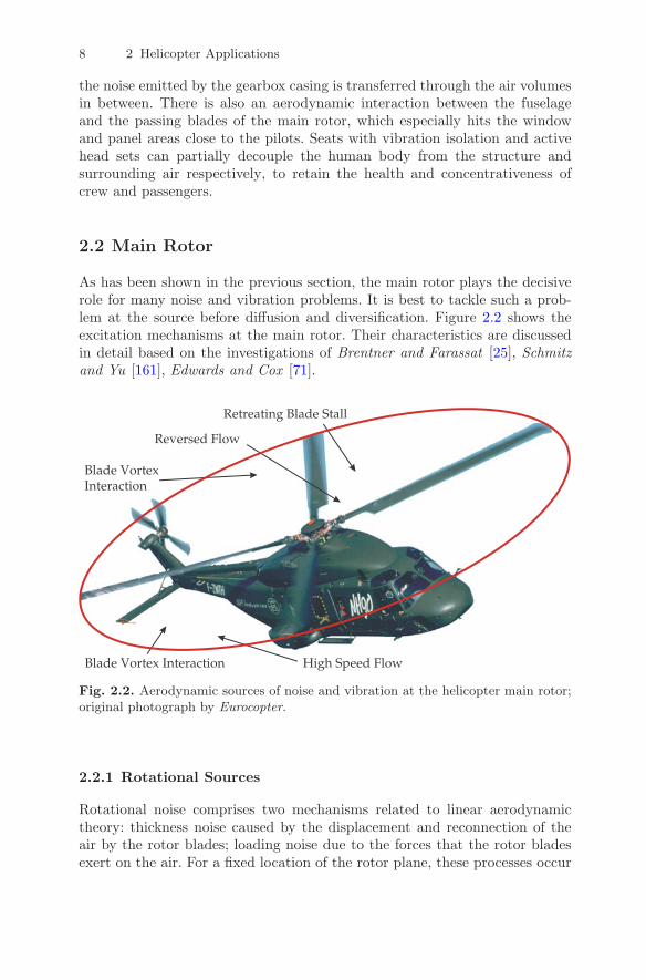
As has been shown in the previous section, the main rotor plays the decisiverole for many noise and vibration problems. It is best to tackle such a prob-lem at the source before diffusion and diversification. Figure 2.2 shows theexcitation mechanisms at the main rotor. Their characteristics are discussedin detail based on the investigations of Brentner and Farassat [25], Schmitzand Yu [161], Edwards and Cox [71].
Fig. 2.2. Aerodynamic sources of noise and vibration at the helicopter main rotor;original photograph by Eurocopter.
2.2.1 Rotational Sources
Rotational noise comprises two mechanisms related to linear aerodynamictheory: thickness noise caused by the displacement and reconnection of theair by the rotor blades; loading noise due to the forces that the rotor bladesexert on the air. For a fixed location of the rotor plane, these processes occur

2.2 Main Rotor 9
periodically with the blade passage frequency, delivering a discrete spectrumwith corresponding higher harmonic frequencies. As both effects depend onthe relative velocity of the blade against the surrounding medium, the soundwaves originate in the forward flight situation from the advancing side of therotor plane and propagate ahead of the blade in the flight direction. Whilethe thickness noise radiates mainly in the rotor plane, the emission of loadingnoise tends slightly downwards.
2.2.2 Impulsive Sources
The impulsive noise of a helicopter leads to several effects with pulsing charac-teristic and high amplitudes at discrete frequencies. Again, we are concernedwith the higher harmonics of the blade passage frequency. These types ofnoise occur in different flight situations and are recognized by the human earas extremely annoying.
Blade Vortex Interaction
As for any airfoil, a vortex wake is shed at the tip of a rotor blade. In for-ward flight, the rotor plane is tilted slightly forward, so these tip vortices donot come into direct contact with the rotor again. In steady descending flighthowever, the blades pass through the tip vortices of their predecessors. Thismeans that the strength and size of the vortex, as well as interaction angle andvertical separation of blade and vortex line are important. Especially whenthey are almost in parallel, the interaction is comparable to a rapid changein the angle of attack with the respective consequences. The effect is aerody-namically similar to ordinary loading noise, but with an impulsive character.Most relevant are the outer blade regions on the advancing side, while bladevortex interaction (BVI) noise is recognizable also on the retreating side. Theradiation takes place below and ahead of the blade.
High Speed Flow Conditions
In forward flight, the blade rotational speed and the flight speed are super-imposed; these components add up on the advancing side of the rotor plane.When this leads to blade tip velocities close to sonic speed, the maximumcruising velocity is reached. In such a critical flow condition, the transonicflow region mainly on the upper side of the airfoil expands with a shock atits end due to compressibility effects. This increases noise radiation and pro-file drag, which is accountable for the induction of vibrations. Just like thethickness noise, the high-speed impulsive (HSI) noise propagates ahead of theblade in the rotor plane.

10 2 Helicopter Applications
Retreating Blade Stall
On the retreating side of the rotor plane, the flight velocity is subtracted fromthe blade rotational speed. This leads, especially at the inner region of therotor blades, to very low flow rates at high angles of attack resulting in stall.Close to the center, the flow is approaching from the backside of the profile.Due to the relatively low velocities, the energy radiated as noise is smallerthan in other impulsive cases. However, the vibrations excited by the periodicand local loss of lift are more noticeable.
2.2.3 Broadband Sources
Broadband noise is essentially generated by random pressure fluctuations onthe blade surface; it can be classified as non-deterministic loading noise. A rea-son for such random pressure fluctuations can be turbulence, existing in thesurrounding atmosphere, caused by the interactions of the preceding blades,or generated on the blade itself. Mechanisms for the latter case are the separa-tion and reattachment of boundary layers, the tip vortex formation, laminarvortex shedding, and trailing edge noise. The directivity of the broadbandnoise is mostly out of the rotor plane.
2.3 Passive Concepts
The examination of the helicopter main rotor has yielded a multitude of exci-tation mechanisms for noise and vibration. Dealing with such a complicatedsystem, it is unlikely that a single solution exists to produce relief in all as-pects. Thus, a variety of partially very different approaches has been discussedand developed. In this section, the major ideas involving non-active elementswill be presented for the classical helicopter configuration. Details on theseelements are given by Bielawa [21], Bramwell et al. [23].
2.3.1 External Devices
As vibrations have historically been the dominant problem and are easier tosolve without a detailed understanding of their generation processes, a numberof devices to improve the situation locally at specific mount points have beendeveloped.
Absorbers
The usual absorber devices consist of mass elements connected by springs orelastic mountings. Often the spring stiffness is provided by the centrifugalforce field, for example in blade-appended pendulum absorbers, shown in Fig-ure 2.3, to compensate out-of-plane loads, or hub attached bifilar absorbers,

2.3 Passive Concepts 11
exemplified in Figure 2.4, for in-plane loads. As an explicit limitation, suchdevices are adjusted to a specific frequency proportional to the rotor speedand thus exhibit only a certain degree of self-tuning. In general, they are rela-tively simple in design and application but introduce additional weight, drag,and maintenance effort for moving parts.
Fig. 2.3. Blade-mounted pendu-lum absorber; original photographby Domke [63].
Fig. 2.4. Hub-mounted bifilar absorber; originalphotograph by Domke [63].
Dampers
The task of damper elements is to reduce the amplitudes of an oscillationbelow a critical margin. Most often they are applied at the blade root inthe lead lag direction, as the oscillations in the rotor plane are only slightlydamped by the aerodynamic forces. Different variants are given in Figures 2.5and 2.6.
Fig. 2.5. Lead lag damper betweenblade attachments; original photographby Domke [63].
Fig. 2.6. Lead lag damper at bladeattachment; original photograph byDomke [63].
2.3.2 Aeroelastic Conformability
When attempting to alter the elastomechanic and aerodynamic behavior ofthe rotor blade with its diverse couplings, and thus the susceptibility to vi-

12 2 Helicopter Applications
bration and noise, complicated interrelations have to be kept in mind. As theblade responds to a composition of several excitation loads, these interrela-tions might lead to a significant reduction or cancellation of vibrations, inprinciple just like an absorber. Regrettably, this composition depends on theflight situation and therefore a beneficial coupling effect for a specific casemight lead to adverse effects in other situations.
Elastomechanic Modifications
There are many parameters that can be adjusted to achieve desired features.A number of tuning/coupling effects can be achieved by the arrangement ofthe neutral axis, principal axes of inertia, or shear center relative to the posi-tion and direction of the loads. Moreover, the exploitation of the anisotropicproperties of fibrous composites allows for additional tailorable couplings. Un-like the traditional rotor blade with almost constant structural properties overthe blade length, future blades may be developed with the aid of advancedcomputational methods to evaluate arbitrary designs.
Aerodynamic Modifications
Similar progress has taken place in the sector of aerodynamics and with in-creasing insight especially into the phenomena of noise generation, more effi-cient blade designs have emerged. As many problems are closely related to theouter blade regions, the blade tip has been object of intense studies. Differentvariants of blade tip shapes are shown in Figure 2.7. Benefits are attainedfor the BVI noise by diffusing the tip vortex, as well as for the HSI noise byreducing the intensity of the transonic flow. For the latter case, a reduction ofthe blade tip speed can be considered at the expense of performance, which
Fig. 2.7. Main rotor blade tip shapes; original photographs by Domke [63].
2.4 Active and Adaptive Concepts 13
then has to be gained by further costly sanctions. Modulated blade spacingis conceptually quite different, see Edwards and Cox [71]. In contrast to thetraditional evenly spaced rotor, several blade passage frequencies with indi-vidual sets of harmonics are generated, and thus the energy is distributed.Practically, this means, for example, that the vortex wakes of the precedingblades are hit with different delays and at different positions.
2.4 Active and Adaptive Concepts
The passive methods available for the reduction of noise and vibration arenot able to achieve completely satisfying results. The most serious drawbackis that they are usually optimal only to a specific situation and are not ableto extend their usefulness in a more general way. This is especially critical inmaneuver flight with rapidly changing conditions which are very difficult topredict. Different concepts involving control systems have been developed foractive intervention, ranging with an increasing degree of structural integrationfrom active, covered by Bielawa [21] and Bramwell et al. [23], to adaptive,discussed for example by Buter [40].
2.4.1 Pitch Control at the Blade Root
In order to achieve equal lift on the advancing and retreating side of the rotorin spite of the unsymmetric flow velocity distribution, the common helicopterconcept makes use of a varying angle of attack. This is introduced with thenecessary cycle duration of one revolution by the swash plate mechanism. Theidea is to actively control the blade pitch, and cancel or reduce the appearingvibrations by superposition of an adequate signal.
Higher Harmonic Control
As most of the characteristic perturbations occur with the blade passage fre-quency and its higher harmonics, the simplest approach is to employ such sig-nals to achieve cancellation. With sensors at relevant points of the airframe,the vibratory load factors are measured and then processed by a control sys-tem. The necessary motion is produced by stationary hydraulic actuators,inducing a vertical displacement of the swash plate and thus a collective ac-tuation of the blades. Such an actuation mechanism may also modify theinclination of the swash plate, but it still is not possible to respond to eventsat an individual blade.
Individual Blade Control
To improve this situation, the blade root actuation mechanism was advancedby inserting hydraulic actuators between the swash plate and blade roots in

14 2 Helicopter Applications
the control rods. With an adequate control algorithm, it would be possibleto implement a very flexible and powerful noise and vibration suppressionsystem. For example, the blade vortex interaction might be alleviated signifi-cantly by steering the blade in the ideal case around the approaching vortex.Admittedly, the expenditure for such a hydraulic system in the rotating partof the rotor hub is very high and therefore has been implemented only inprototype aircraft.
2.4.2 Discrete Flap Actuation
Apart from further development of control algorithms, there is a need for effi-cient actuation mechanisms. The integration of flaps into rotor blades presentssome challenges. In order to be aerodynamically effective, the interventionneeds to be located in the outer blade region, where extreme centrifugal loadsare present. Moreover, spatial restrictions apply there, and the mass distribu-tion preferably should not be altered. Under these conditions, the applicationof hydraulic systems is hardly conceivable, and multifunctional materials comeinto operation. Piezoelectric ceramics with their dynamic capabilities over abroad frequency range are used for such actuators. Different configurationshave been in discussion or realized, like leading or trailing edge flaps, as shownin Figure 2.8, and the related active blade tips. Still, a discrete flap alwaysdisturbs the air flow and consequently reduces the aerodynamic performance,particularly in the extreme flow conditions exhibited by a helicopter rotor.Although the actuators themselves are designed to operate without too manymoving parts, quite a few hinges and connections are necessary and theseincrease complexity and maintenance effort.
Fig. 2.8. Experimental rotor blade with trailing edge flaps; from Kloppel et al. [112].
2.4.3 Integral Blade Actuation
Multifunctional materials are currently not able to provide the performanceneeded for blade-root actuation. In order to influence the aerodynamically

2.5 Adaptive Beam Aspects 15
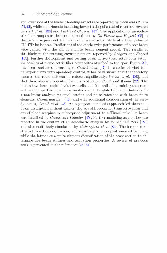
interesting outer region of the blades, they can be applied to induce twist ormanipulate the blade shape in other ways. A number of schemes to twist theblades have been developed involving directionally attached monolithic piezo-electric ceramics or passive couplings of the anisotropic blade skin to convertthe excitation of an actuator. The highest degree of integration is reached withthe distributed application of piezoelectric fiber composites, see Figure 2.9,with tailorable active, sensoric, and passive properties. In such a configura-tion, adaptive layers are used as, or merged into, the blade skin and thereforeprovide actuation authority without moving parts or flow disturbance, andwith only a minor weight penalty as they contribute to the passive structuralbehavior. Certain limitations in the material properties have to be consideredfor piezoelectric fibers. Due to their ceramic nature, they are relatively brittleand should carry loads in compression rather than in tension.
Fig. 2.9. Scaled active twist rotor blade with piezoelectric fiber composite patchesattached to the spar; from Cesnik [44].
2.5 Adaptive Beam Aspects
In this discussion, the integral blade actuation has been identified to be apromising development direction to alleviate noise and vibration problemsof rotorcraft in the long term. While other technologies based on conven-tional materials or designs are closer to the market introduction, fundamentalquestions need to be answered with regard to material science and struc-tural mechanics for the integral blade actuation. Thus, the focus of researchis placed upon the application of adaptive fiber composites because of theirversatile adjustable capabilities. With these it is possible to induce displace-ments or rotations with respect to the blade axis as well as deformations inthe cross-sectional plane. The latter, also known as chamber variation, mightbe of interest for fixed-wing aircraft but is improbable for implementationon rotating-wing aircraft due to the complex load and excitation situation ofthe blade structure. Such a slender structure can be efficiently idealized as abeam. Further on, the set-up of a rotor blade with foam-filled chambers willrequire modeling by means of a thin-walled beam. Thus, an adequate andcomprehensive theoretical framework for adaptive thin-walled beams will bedeveloped here.

16 2 Helicopter Applications
2.5.1 Beam Actuation Concepts
In Section 2.2, the essential noise and vibration phenomena occurring at thehelicopter main rotor have been analyzed. They lead to bending oscillationsof the blades, which may be modeled by thin-walled beams. Equipping such astructure with adaptive fiber composites permits different actuation schemesto compensate for bending-related displacements, see Figure 2.10. It is pos-sible to accomplish this for static operation by inducing opposing displace-ments. Such bending actuation may be realized directly through expansionand contraction of opposing wall sectors and through shear deformation oftransversely oriented wall sectors. Alternatively, coupling effects due to con-stitutive anisotropy of the walls may be exploited, for example transforminga lengthwise expansion of piezoelectric layers, which is applied consistentlythroughout the cross-section, into the desired beam bending. In a rotatingenvironment, it is possible to amplify the rather small attainable displace-ments with the aid of aerodynamic forces. Since a small change in the angleof attack may lead to a significant change in lift and drag with the associatedblade displacements, twist actuation becomes important. It can be achievedagain either directly through the consistent induction of shear in the wallsor via structural couplings related to the constitutive anisotropy of the wallsas well as to the warping of the cross-section. The prior couples, for exam-ple, extension with torsion and the latter warping with torsion. Naturally,not all of the various actuation schemes are equally suitable for reducing thehelicopter rotor problems. The research reported in the literature is clearlyfocused upon the direct torsion, see Section 2.5.3. Here a general approach
Fig. 2.10. Actuation schemes for the reduction of beam-bending oscillations inconsideration of aerodynamic forces in a rotating environment.

2.5 Adaptive Beam Aspects 17
will be developed, capable of describing all potential actuation schemes bymeans of a single theory of thin-walled beams incorporating adaptive fibercomposites.
2.5.2 Adaptive System Concepts
Since the piezoelectric effect comprises two aspects, direct and converse, com-posites with such properties may be used for both sensing and actuation.Combining these two with a control unit makes an adaptive system. Bothactuators and sensors may be either discrete, at a specific location, or inte-gral, spatially distributed. The latter case typically can be accomplished withpiezoelectric fiber composites. Figure 2.11 illustrates the possible combina-tions with elementary control schemes. Using open-loop control, a signal forthe actuator is prescribed based on knowledge about the system. For a he-licopter rotor, this usually involves higher harmonic frequencies, sufficientlycovering a constant flight condition. For more versatile tasks, correspondingto changing flight conditions, closed-loop control provides actuator signals inresponse to sensor signals. Such control concepts for helicopter rotor bladeshave mainly been developed for pitch actuation at the blade root or the trail-ing edge flap, see for example Konstanzer [115]. Further on in Figure 2.11,passive control stands for the use of piezoelectric material with inductive res-onant, resistive, capacitive, and switched shunt circuits, see Lesieutre [122].A shunt circuit with a combination of resistance and inductance allows usto induce tunable damping and absorption of vibrations. The suitability ofpiezoelectric fiber composites for such an application has been demonstratedby Adachi et al. [3]. A single element acts in turn as actuator and sensor.For better efficiency, it should be of integral type, since neither electric noraeroelastic amplification can be utilized.
Fig. 2.11. Control of beam oscillations.
2.5.3 Development Status
The initial examinations of directly induced torsion were conducted for mono-lithic piezoelectric ceramics being attached in a ±45◦ direction to the upper
18 2 Helicopter Applications
and lower side of the blade. Modeling aspects are reported by Chen and Chopra[51,52], while experiments including hover testing of a scaled rotor are coveredby Park et al. [138] and Park and Chopra [137]. The application of piezoelec-tric fiber composites has been carried out by Du Plessis and Hagood [65] intheory and experiment by means of a scaled rotor blade of a Boeing-VertolCH-47D helicopter. Predictions of the static twist performance of a box beamwere gained with the aid of a finite beam element model. Test results ofthis blade in the rotating environment are reported by Rodgers and Hagood[155]. Further development and testing of an active twist rotor with actua-tor patches of piezoelectric fiber composites attached to the spar, Figure 2.9,has been conducted according to Cesnik et al. [47]. In a series of wind tun-nel experiments with open-loop control, it has been shown that the vibratoryloads at the rotor hub can be reduced significantly, Wilbur et al. [180], andthat there also is a potential for noise reduction, Booth and Wilbur [22]. Theblades have been modeled with two cells and thin walls, determining the cross-sectional properties in a linear analysis and the global dynamic behavior ina non-linear analysis for small strains and finite rotations with beam finiteelements, Cesnik and Shin [46], and with additional consideration of the aero-dynamics, Cesnik et al. [48]. An asymptotic analysis approach led them to abeam description without explicit degrees of freedom for transverse shear andout-of-plane warping. A subsequent adjustment to a Timoshenko-like beamwas described by Cesnik and Palacios [45]. Further modeling approaches arereported in the context of an aeroelastic analysis by Wilkie and Park [181]and of a multi-body simulation by Ghiringhelli et al. [82]. The former is re-stricted to extension, torsion, and structurally uncoupled uniaxial bending,while the latter use a finite element discretization of the cross-section to de-termine the beam stiffness and actuation properties. A review of previouswork is presented in the references [26–37].

3
Fundamental Considerations
This chapter describes the fundamental theories for investigating physical sys-tems with regard to deformable structures and dielectric domains as examinedby mechanics and electrodynamics, respectively, within the field of theoreticalphysics, see for example Schaefer and Pasler [160]. It clarifies the essentialinterrelations and provides a consistent basis to serve as a reference for thesubsequent chapters, where more detailed and specific models will be devel-oped.
3.1 Mathematical Preliminaries
For the required representation of the laws of physics independent of a specialcoordinate system, tensor calculus is invaluable. As matrix calculus is quiteconvenient with regard to component representation and implementation, itshall be employed when applicable. The tensor- and the matrix-based observa-tion concept include or depict vector algebra. We assume that the mathemati-cal fundamentals are known and therefore give only a fragmentary overview toclarify notation and to introduce utilized rules and conventions. A useful andcomprehensive collection of formulas is given by Rade and Westgren [147],while the tensors are the subject of Sokolnikoff [167], Prager [144], Itskov[105], Brunk and Kraska [38] as well as the matrices of Lax [119], Zurmuhland Falk [188].
3.1.1 Euclidean Vectors
The examinations will be accomplished in the three-dimensional Euclideanvector space, where the scalar product of vectors is defined beyond the prop-erties of the affine space. Cartesian coordinates with their orthogonal, straight,and normalized base are sufficient for the problems at hand and therefore willbe used.
T.H. Brockmann, Theory of Adaptive Fiber Composites,Solid Mechanics and Its Applications 161,c© Springer Science + Business Media B.V. 2009

20 3 Fundamental Considerations
Vectorial Products
The scalar or dot product processes two vectors, for example v and w, ofarbitrary dimension into a scalar. The scalar product is commutative:
v · w =
⎧⎨
⎩
v1v2. . .
⎫⎬
⎭·
⎧⎨
⎩
w1
w2
. . .
⎫⎬
⎭= v1w1 + v2w2 + · · · , v · w = w · v. (3.1)
The vector or cross product determines a so-called axial vector with orthogonalorientation from two spatial vectors. The vector product is anti-commutative:
v × w =
⎧⎨
⎩
v1v2v3
⎫⎬
⎭×
⎧⎨
⎩
w1
w2
w3
⎫⎬
⎭=
⎧⎨
⎩
v2w3 − v3w2
v3w1 − v1w3
v1w2 − v2w3
⎫⎬
⎭, v × w = −w × v. (3.2)
3.1.2 Tensor Representation
With the chosen type of coordinates and for the sake of simplicity, it canbe abstained from the index notation. The classification of tensors with theapplied typesetting conventions is given in Table 3.1.
Table 3.1. Tensors of different order.
Order Denotation Example
0th scalar s1st vector v, w
2nd dyad c,d
nth general tensor
Tensorial Products
The double contracting or double inner product of general tensors resultsin a tensor with the added order of the multiplied tensors lowered by four.The employed symbol of two dots alludes to the two scalar products of theparticular base vectors. In the case of two tensors of second order, the outcomeis of zeroth order, leading to the denomination as a scalar product of dyads.The double contracting product is commutative, given here for the case ofdyads:
c · · d = d · · c. (3.3)
When only a single scalar product of base vectors is involved, the result ofsuch a product has the added order of the multiplied tensors lowered by two.This contracting or inner product of general tensors thus comprises the scalarproduct of vectors as a special case. Further on, the tensorial or outer product

3.1 Mathematical Preliminaries 21
of general tensors leads to a result with a summed order of the multipliedtensors. Therefore, its application to vectors results in a dyad, giving reasonto the denomination as the dyadic product of vectors often indicated by thesymbol ⊗. The contracting product, Eq. (3.4a), and the tensorial product,Eq. (3.4b), of general tensors are non-commutative:
v · d �= d · v, (3.4a)vd �= dv. (3.4b)
For the occurrence of a transposed dyad within consecutive contracting prod-ucts, the following rearrangement is permissible:
(dT · v
)· w = v · (d · w) . (3.5)
Theorems
Concerning the partial differentiation of tensors, the following abbreviationsfor gradient and divergence are introduced:
grad(·) = �(·),div(·) = �(·).
For the manipulation of equations with products containing these operators,Gauss’s divergence theorem will be needed. It is given for the usual case withthe product of a scalar and a vector in Eq. (3.6a) and for the contractingproduct of a transposed dyad and a vector in Eq. (3.6b):
� (sv) = s�v + v · �s, (3.6a)�(dT · v
)= v · �d + d · ·�v. (3.6b)
When Λ is a spatial domain with the closed boundary ∂Λ and the respectiveunit vector field of the surface normals en is directed outwards, then Gauss’sintegral theorem states
∫
Λ
�v dV =∫
∂Λ
v · dA =∫
∂Λ
v · en dA. (3.7)
3.1.3 Matrix Representation
Depending on the circumstances, it makes sense to apply either tensor ormatrix calculus. Occasionally it may be useful to switch the representation.Typically, the results of a derivation requiring tensors are written in the moreaccessible matrix form. While operations involving scalars and vectors areapplicable for both, the more general case is subjected to restrictions:
• A tensor of second order may be represented by a square matrix, but ageneral non-square matrix cannot be represented by a tensor.

22 3 Fundamental Considerations
• A tensor of more than second order cannot be represented by a singlematrix without rearrangement of components.
However, the latter statement implies that tensors can be converted to matri-ces involving the rearrangement of components. Therewith tensors of secondorder may be expressed by column matrices, also referred to as vectors. Thiswill be implemented in the following section for stresses and strains. Theclassification of matrices with the applied typesetting conventions is given inTable 3.2.
Table 3.2. Matrices of different dimensions.
Dimension Denotation Example
column vector v, w
row transposedvector vT , wT
general matrix m
Substitution of Vectorial Products
Usually within the framework of matrix calculus, the vector operations areretained or may be replaced with pure matrix algebra. In matrix notation,the scalar product of two vectors may be represented by the matrix productof a row and a column matrix:
v · w = w · v ↔ vT w = wT v. (3.8)
For the vector product, the components of one of the vectors need to berearranged into a skew-symmetric matrix and then multiplied with the columnmatrix of the other:
v × w ↔ 〈v〉 w = 〈w〉Tv
with v =
⎧⎨
⎩
v1v2v3
⎫⎬
⎭↔ 〈v〉 = − 〈v〉T =
⎡
⎣0 −v3 v2v3 0 −v1
−v2 v1 0
⎤
⎦ . (3.9)
3.2 Deformable Structures–Mechanical Fields
A mechanical system may consist of several different parts. When such a partis able to undergo deformations, it will be regarded as a deformable structure.It may be modeled with a certain complexity, for example with the aid ofshell or beam theory, but can be traced back to the basic configuration ofthe continuum, which is the subject of investigation within the homonymousbranch of mechanics. Such a continuum is a continuous domain of spatial,

3.2 Deformable Structures–Mechanical Fields 23
planar, or linear extent filled with matter. It consists of elements denominatedas particles, which are small in the macroscopic view and thus mathematicallypoint-shaped but ample in the microscopic view compared with the materialstexture. Introductory literature for this topic is given, for example, by Beckerand Gross [9] as well as beyond by Wempner [177], Green and Zerna [88],Sokolnikoff [166].
3.2.1 Loads
Loads may be distinguished with respect to the location of their origin andnature of their action. External loads act from the outside of the mechanicalsystem, while the internal loads appear within, and become visible when thesystem is cut. Applied or physical loads are regarded as given, whereas reactiveor geometric loads are initially unknown, and result from restrictions on themotion and deformation. Loads may act upon a volume, a surface, or in ideallimit cases as line or point loads. They are representable by tensors of firstorder, thus taking the form of vectors. For a force F affecting a volume or anarea, the vector fields of force density with a volume force f or an area forcef describe the three- or two-dimensional distribution respectively:
f =dF
dV, (3.10a)
f =dF
dA. (3.10b)
While forces and moments are considered for the general mechanical system,the continuum usually is limited to the introduction of the concept of forces.From this point of view, the Cosserat theory is mentioned here as an exception,see Rubin [157] for details.
3.2.2 Stresses
The loading of a continuum due to external forces is characterized by thestresses observed at the individual particles. When the continuum is cut, theinternal force dF at a particle is found to be acting upon the associated surfaceelement dA in the section plane. The stress vector f can then be definedin accordance with Eq. (3.10b). The stress tensor σ again results from thestress vectors of three orthogonal section planes unfolding between the unitvectors e1, e2, e3 of the Cartesian coordinate system. Given by Eq. (3.11),it is commonly denominated as the Cauchy stress tensor and is of secondorder. Demanding the local balance of moments, its symmetry can be shownas elucidated by Figure 3.1. An alternative representation may be gained byresorting the six remaining independent components into a vector as of theright-hand side of Eqs. (3.12).

24 3 Fundamental Considerations
σ =[f1 f2 f3
]T, (3.11)
σ = σT =
⎡
⎣σ1 τ12 τ31τ12 σ2 τ23τ31 τ23 σ3
⎤
⎦ ↔ σ =
⎧⎪⎪⎪⎪⎪⎪⎨
⎪⎪⎪⎪⎪⎪⎩
σ1
σ2
σ3
τ23τ31τ12
⎫⎪⎪⎪⎪⎪⎪⎬
⎪⎪⎪⎪⎪⎪⎭
. (3.12)
In turn it is possible to deduce the stress vector fn acting upon a surface withthe unit normal vector en from the stress tensor. Such an equilibrium relationis especially useful when it comes to the description of boundary conditions.This is the Cauchy theorem:
fn = σ · en ↔ fn = σT en. (3.13)
Fig. 3.1. Stress vectors with associated components by means of an infinitesimalvolume element.
3.2.3 Mechanical Equilibrium
Transitioning from the stress state of a particle to the stress field of the contin-uum, the interaction of the Cauchy stress tensor components of neighboringpoints needs to be investigated. They have to satisfy the conditions of localequilibrium to be established with the aid of an arbitrary infinitesimal volumeelement. Such an element with faces in parallel to the planes of the Cartesiancoordinate system is subjected to the volume force fΛ and on the faces tothe components of the Cauchy stress tensor with additional increments in theform of the first element of Taylor expansions on one of the respective oppos-ing faces. The balance of moments proves the symmetry of the stress tensor,

3.2 Deformable Structures–Mechanical Fields 25
whereas the balance of forces leads to the equation of internal mechanicalequilibrium
�σ + fΛ = 0 in Λ. (3.14)
Here the continuum is denoted by the domain Λ and the respective boundary∂Λ is subdivided to consider two types of boundary conditions. The area ∂Λσ
is subjected to the prescribed loads f∂Λ of the physical boundary conditionsin equilibrium with the boundary stresses expressed by application of theCauchy theorem of Eq. (3.13) (Neumann boundary conditions):
f∂Λ = σ · en on ∂Λσ. (3.15)
The prescribed displacements u∂Λ of the geometric boundary conditions areimposed on the area ∂Λu (Dirichlet boundary conditions):
u∂Λ = u on ∂Λu. (3.16)
3.2.4 Strains
The deformation of a continuum may be described by the displacement u ofits particles and their strain state. For that purpose, it is convenient to dis-tinguish between the initial configuration of the undeformed and the currentconfiguration of the deformed body. A particle can be identified either by itsoriginal position X in the initial configuration, Figure 3.2(a), thus trackingthe particle’s individual state at subsequent positions, or by its momentaryposition x in the current configuration, Figure 3.2(b), thus tracking the stateof subsequent particles at this fixed position. The former is the Lagrangianapproach, the latter case is called the Eulerian approach. The strain field ofthe continuum may be expressed by the difference of the squared lengths of a
Fig. 3.2. Deformation of a continuum—(a) reference configuration with particleposition X and (b) momentary configuration with particle position x in the inertialframe of reference.
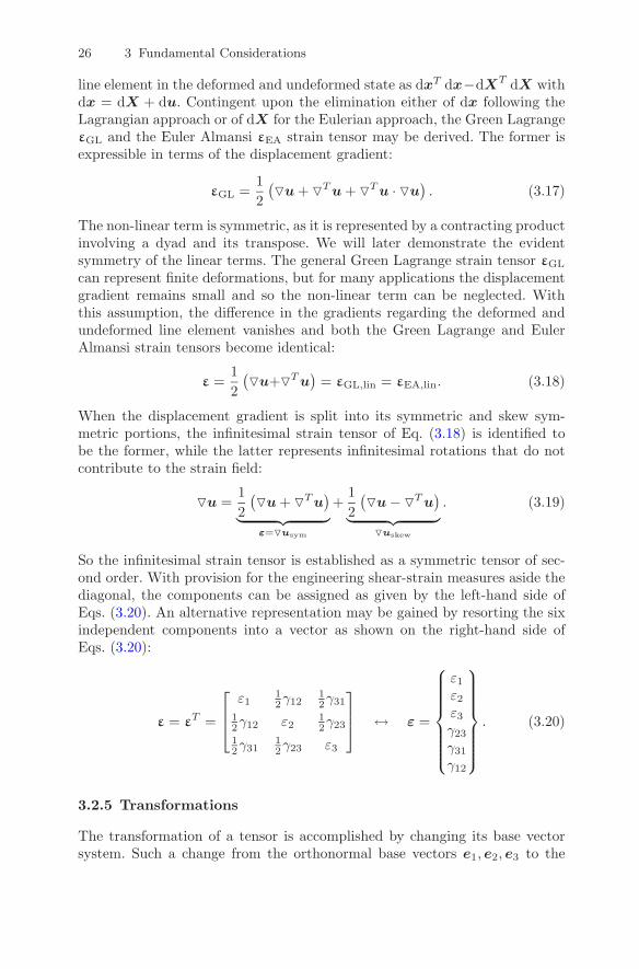
26 3 Fundamental Considerations
line element in the deformed and undeformed state as dxT dx−dXT dX withdx = dX + du. Contingent upon the elimination either of dx following theLagrangian approach or of dX for the Eulerian approach, the Green LagrangeεGL and the Euler Almansi εEA strain tensor may be derived. The former isexpressible in terms of the displacement gradient:
εGL =12(�u + �T u + �T u · �u
). (3.17)
The non-linear term is symmetric, as it is represented by a contracting productinvolving a dyad and its transpose. We will later demonstrate the evidentsymmetry of the linear terms. The general Green Lagrange strain tensor εGL
can represent finite deformations, but for many applications the displacementgradient remains small and so the non-linear term can be neglected. Withthis assumption, the difference in the gradients regarding the deformed andundeformed line element vanishes and both the Green Lagrange and EulerAlmansi strain tensors become identical:
ε =12(�u+�T u
)= εGL,lin = εEA,lin. (3.18)
When the displacement gradient is split into its symmetric and skew sym-metric portions, the infinitesimal strain tensor of Eq. (3.18) is identified tobe the former, while the latter represents infinitesimal rotations that do notcontribute to the strain field:
�u =12(�u + �T u
)
︸ ︷︷ ︸ε=�usym
+12(�u − �T u
)
︸ ︷︷ ︸�uskew
. (3.19)
So the infinitesimal strain tensor is established as a symmetric tensor of sec-ond order. With provision for the engineering shear-strain measures aside thediagonal, the components can be assigned as given by the left-hand side ofEqs. (3.20). An alternative representation may be gained by resorting the sixindependent components into a vector as shown on the right-hand side ofEqs. (3.20):
ε = εT =
⎡
⎢⎣
ε112γ12
12γ31
12γ12 ε2
12γ23
12γ31
12γ23 ε3
⎤
⎥⎦ ↔ ε =
⎧⎪⎪⎪⎪⎪⎪⎨
⎪⎪⎪⎪⎪⎪⎩
ε1ε2ε3γ23γ31γ12
⎫⎪⎪⎪⎪⎪⎪⎬
⎪⎪⎪⎪⎪⎪⎭
. (3.20)
3.2.5 Transformations
The transformation of a tensor is accomplished by changing its base vectorsystem. Such a change from the orthonormal base vectors e1, e2, e3 to the

3.2 Deformable Structures–Mechanical Fields 27
arbitrarily rotated orthonormal base vectors es, en, ex may be expressed withthe aid of transformation coefficients in the form of directional cosines betweenthese vectors, Eq. (3.21a), respectively, their scalar products, Eq. (3.21b):
cai = cos (ea, ei) with a ∈ [s, n, x] and i ∈ [1, 2, 3] , (3.21a)
cai = ea · ei ↔ cai = eTa ei. (3.21b)
These transformation coefficients may be summarized in the transformationmatrix T for the subsequent transformation of stresses, respectively strains,in matrix representation:
⎧⎪⎪⎪⎪⎪⎪⎨
⎪⎪⎪⎪⎪⎪⎩
σs
σn
σx
τnx
τxs
τsn
⎫⎪⎪⎪⎪⎪⎪⎬
⎪⎪⎪⎪⎪⎪⎭
︸ ︷︷ ︸σ(s,n,x)
= T
⎧⎪⎪⎪⎪⎪⎪⎨
⎪⎪⎪⎪⎪⎪⎩
σ1
σ2
σ3
τ23τ31τ12
⎫⎪⎪⎪⎪⎪⎪⎬
⎪⎪⎪⎪⎪⎪⎭
︸ ︷︷ ︸σ(1,2,3)
,
⎧⎪⎪⎪⎪⎪⎪⎪⎨
⎪⎪⎪⎪⎪⎪⎪⎩
εsεnεx
12γnx
12γxs
12γsn
⎫⎪⎪⎪⎪⎪⎪⎪⎬
⎪⎪⎪⎪⎪⎪⎪⎭
= T
⎧⎪⎪⎪⎪⎪⎪⎪⎨
⎪⎪⎪⎪⎪⎪⎪⎩
ε1ε2ε3
12γ2312γ3112γ12
⎫⎪⎪⎪⎪⎪⎪⎪⎬
⎪⎪⎪⎪⎪⎪⎪⎭
. (3.22)
As it is dealt with second-order tensors, the associated base vector pairs needto be considered, and thus products of the transformation coefficients appearin the transformation matrix:
T =
⎡
⎢⎢⎣
c2s1 c2
s2 c2s3 2cs2cs3 2cs3cs1 2cs1cs2
c2n1 c2
n2 c2n3 2cn2cn3 2cn3cn1 2cn1cn2
c2x1 c2
x2 c2x3 2cx2cx3 2cx3cx1 2cx1cx2
cs1cn1 cs2cn2 cs3cn3 cs2cn3 + cn2cs3 cs1cn3 + cn1cs3 cs1cn2 + cn1cs2cs1cx1 cs2cx2 cs3cx3 cs2cx3 + cx2cs3 cs1cx3 + cx1cs3 cs1cx2 + cx1cs2cn1cx1 cn2cx2 cn3cx3 cn2cx3 + cx2cn3 cn1cx3 + cx1cn3 cn1cx2 + cx1cn2
⎤
⎥⎥⎦ .
(3.23)A significant simplification is to be noted when the rotation is performedaround a common base vector. Thus, for example, for a rotation α around thecoincident vectors e2 and en, the transformation coefficients take the followingform:
cs1, cx3 = cosα, cx1 = cos(π
2+ α
), cs3 = cos
(π
2− α
), (3.24a)
cn2 = cos 0, cn1, cs2, cx2, cn3 = cosπ
2. (3.24b)
Therewith the transformation matrix reduces to
T =
⎡
⎢⎢⎢⎢⎢⎢⎣
cos2 α 0 sin2 α 0 −2 sinα cosα 00 1 0 0 0 0
sin2 α 0 cos2 α 0 2 cosα sinα 00 0 0 − sinα 0 cosα
cosα sinα 0 − sinα cosα 0 cos2 α − sin2 α 00 0 0 cosα 0 sinα
⎤
⎥⎥⎥⎥⎥⎥⎦
.
(3.25)

28 3 Fundamental Considerations
As visible on the right-hand side of Eqs. (3.22), the transformation of strainsdoes not yet cope with the engineering shear-strain measures introduced inthe previous subsection. This can be accomplished, as shown for the planarcase by Jones [107], by multiplication with the correction matrix R:
⎧⎪⎪⎪⎪⎪⎪⎨
⎪⎪⎪⎪⎪⎪⎩
εsεnεxγnx
γxs
γsn
⎫⎪⎪⎪⎪⎪⎪⎬
⎪⎪⎪⎪⎪⎪⎭
︸ ︷︷ ︸ε(s,x,n)
= R
⎧⎪⎪⎪⎪⎪⎪⎨
⎪⎪⎪⎪⎪⎪⎩
εsεnεx
12γnx12γxs12γsn
⎫⎪⎪⎪⎪⎪⎪⎬
⎪⎪⎪⎪⎪⎪⎭
,
⎧⎪⎪⎪⎪⎪⎪⎨
⎪⎪⎪⎪⎪⎪⎩
ε1ε2ε3γ23γ31γ12
⎫⎪⎪⎪⎪⎪⎪⎬
⎪⎪⎪⎪⎪⎪⎭
︸ ︷︷ ︸ε(1,2,3)
= R
⎧⎪⎪⎪⎪⎪⎪⎨
⎪⎪⎪⎪⎪⎪⎩
ε1ε2ε3
12γ2312γ3112γ12
⎫⎪⎪⎪⎪⎪⎪⎬
⎪⎪⎪⎪⎪⎪⎭
,
with R =
⎡
⎢⎢⎢⎢⎢⎢⎣
1 0 0 0 0 00 1 0 0 0 00 0 1 0 0 00 0 0 2 0 00 0 0 0 2 00 0 0 0 0 2
⎤
⎥⎥⎥⎥⎥⎥⎦
. (3.26)
When these equations are utilized for the strain transformation relation onthe right-hand side of Eqs. (3.22), the transformation matrix is multipliedfrom the left by the correction matrix and from the right by its inverse. Forthe rotation around a common base vector, it is straightforward to show thatthis results in a transposed and inverted transformation matrix:
ε (s, x, n) = RTR−1ε (1, 2, 3) =(TT
)−1ε (1, 2, 3) . (3.27)
Complementarily, the stress transformation relation of the left-hand side ofEqs. (3.22) will be given in the corresponding form:
σ (s, n, x) = Tσ (1, 2, 3) . (3.28)
3.3 Dielectric Domains–Electrostatic Fields
In contrast to conductive material with the ability to accommodate electricflow fields, dielectric matter, as well as vacuum, may exhibit electrostaticfields. Although the physical condition of the examined dielectric domain isnot limited to solid state, it may be described in analogy with deformablestructures as a continuum. In comparison to the mechanical fields, the tensorscharacterizing the electrostatic fields will be one order lower. A comprehensivedescription of electrical engineering is given by Paul [140], while electromag-netic fields are detailed by Fischer [74], Lehner [120], and Reitz et al. [153].

3.3 Dielectric Domains–Electrostatic Fields 29
3.3.1 Electric Charge
Length, mass, and time are the elementary quantities of mechanics. For elec-tric phenomena, they have to be complemented with the electric charge Q.The charge of particles, usually denominated as charge carriers, implicates arepulsive or attractive force between them for charges of identical or oppositesign, respectively. When charge is distributed over a volume or an area, thescalar fields of the electric charge density with volume charge q or area chargeq describe the three- or two-dimensional distribution, respectively:
q =dQdV, (3.29a)
q =dQdA. (3.29b)
With the exception of the limit case of vacuum, a dielectric holds chargecarriers just like a conductor. The substantial difference and reason for thedistinct types of electric fields is that in the dielectric the charge carriers arenot able to move. Thus, the induced electric field is static, although magnitudeand direction may change due to variable charges.
3.3.2 Electric Flux Density
The electrostatic field expands between charges separated by a dielectric andmay be illustrated by the lines of electric flux connecting them. Positive andnegative charges are sources and drains of the electric flux. So the electricflux only depends on the charges but not on the dielectric. The contributionof a charge Q can be expressed by the integral of the electric flux density D,occasionally also denoted electric displacement, over an arbitrary enclosingenvelope with the surface normal en in an outward direction:
Q =∮
D · dA → dQ = D · dA = D · en dA. (3.30)
This is the Gaussian law of electrostatics in integral and differential form. Thelatter may be reorganized to express the electric flux density with the aid ofthe charge density of the dedicated area, as given by Eq. (3.29b), leading tothe equivalent of the Cauchy theorem of mechanics from Eq. (3.13):
dQdA
= q = D · en = DT en. (3.31)
3.3.3 Electrostatic Equilibrium
The charge affecting the surrounding domain Λ may be expressed in termsof the spatial charge density through integration of Eq. (3.29a) as well as in

30 3 Fundamental Considerations
terms of the electric flux density on its boundary ∂Λ given by the Gaussianlaw in Eq. (3.30):
Q =∫
Λ
qΛ dV, (3.32a)
Q =∫
∂Λ
D · dA. (3.32b)
The surface integral in Eq. (3.32b) can be transformed into a volume integralover the enclosed domain by using Gauss’s integral theorem, Eq. (3.7). Equat-ing with Eq. (3.32a) leads to the electrostatic equilibrium condition, which isknown as one of Maxwell’s equations in integral form:
∫
Λ
qΛ dV =∫
Λ
�D dV . (3.33)
As the considered domain may be arbitrarily chosen, this relationship betweenspatial charge density and divergence of flux density needs to be satisfied atevery point. Thus, the differential form of Maxwell’s equation can be obtained:
�D − qΛ = 0 in Λ. (3.34)
Just as in the mechanical case, the boundary ∂Λ of the dielectric domain Λis subdivided to consider two types of boundary conditions. The equilibriumbetween prescribed charges q∂Λ on the area ∂ΛD and the electric flux densitycan be established with Eq. (3.31). Since these charges are located on theoutside, the appearing normal vector en is pointing inward. Thus, for anoutward oriented surface normal en = −en on the boundary of the dielectricdomain, it may be written as
−q∂Λ = D · en on ∂ΛD. (3.35)
For the area ∂Λϕ, the electric potential ϕ∂Λ is prescribed as
ϕ∂Λ = ϕ on ∂Λϕ. (3.36)
3.3.4 Electric Field Strengths
The vector field of electric field strength E represents the force action of thecharges already mentioned in Section 3.3.1. It is defined as the ratio of thevector of exerted force F and scalar of causative charge Q at every pointwithin the field
E =F
Q. (3.37)
The work dW performed by a force along the differential distance vector dsis formulated in Eq. (3.38a). Assuming that the considered field is a poten-tial function field and thus irrotational, the work done by a charge may be
3.4 Principle of Virtual Work 31
expressed as of Eq. (3.38b):
dW = F · ds, (3.38a)dW = −Q dϕ. (3.38b)
Equating Eqs. (3.38a) and (3.38b) and couching the relation of force andcharge as of Eq. (3.37), the electric field strength E may be determined asa function of the electric potential ϕ after auxiliary expansion with the unitvector es of the above-mentioned differential distance vector ds:
E · ds = −dϕ,E dses · es = −dϕes,
E = − dϕds
es = −�ϕ.(3.39)
Examining a single component Ei of the electric field strength vector E, itmay be described for a linear electric potential distribution between two pointswith the potentials ϕa and ϕb and the distance vector component si in theregarded direction by
Ei = −ϕb − ϕa
si. (3.40)
3.4 Principle of Virtual Work
The field of analytical mechanics is characterized by variational principles pos-tulated as axioms and dealing with scalar quantities like work or energy. Inaddition to the actual states of the mechanical system, there are virtual states,which in general are supposed to be independent of time, small, and admissi-ble, but notional: they do not necessarily have to occur. From the mathemat-ical point of view, these virtual states represent test functions. While for thecase of actual quantities, the letter “d” is usually used to indicate differentiallysmall values, such virtual values are denoted with the symbol “δ” followingthe notation in the calculus of variations. This approach can be applied to theelectric properties of a system, too. The principles of mechanics may be foundin Pasler [139], Budo [39], Lanczos [118], Szabo [172], or Dym and Shames[70], while the extension to coupled electrostatic fields is accredited to Hollandand EerNisse [100] and given, for example, by Ghandi and Hagood [81].
3.4.1 General Principle of Virtual Work
This fundamental principle of physics is given by the axiom of Remark 3.1 inits most general formulation, where δW is the total virtual work of the system.For mechanical fields in deformable structures as well as for electrostatic fieldsin dielectric domains, it can be restated by the equality of internal δU andexternal δV contributions.

32 3 Fundamental Considerations
Remark 3.1. A physical system will be in equilibrium only if the total virtualwork in accordance with the admissibility criteria vanishes.
δW = δU − δV = 0. (3.41)
Mechanical work at every particle of a continuum results from acting forceand respective displacement or local stress and strain. correspondingly. So theabove axiom of Remark 3.1 actually comprises two principles involving eithervirtual loads or virtual displacements. A brief derivation of both will be givenin the following subsections. Similarly, the electric work can be treated, butwe will present only one of the variants. The different formulations of theprinciple of virtual work are independent of a constitutive law and may bedenoted as the weak forms of equilibrium, as only the equilibrium conditionshave to be fulfilled in the integral mean. Weaker requirements with regardto differentiability of the involved functions have to be fulfilled, since theorder of derivatives is reduced in comparison to the equilibrium formulationof Eqs. (3.14) and (3.34).
3.4.2 Principle of Virtual Displacements
The mechanical equilibrium of an infinitesimal volume element of a deformablestructure, given by Eq. (3.14), may be multiplied with the vector field ofvirtual displacements δu and integrated over the domain Λ yielding
∫
Λ
δu · (�σ + fΛ) dV = 0. (3.42)
Separation of the terms leads to Eq. (3.43a), where the first term can be splitinto two parts with the aid of the divergence product rule of Eq. (3.6b), asshown in Eq. (3.43b). With the commutativity of the terms in the first inte-grand according to Eq. (3.3) and application of Gauss’s integral theorem ofEq. (3.7) to the second integrand, while interchanging the multipliers accord-ing to Eq. (3.5), the formulation of Eq. (3.43c) is reached:
∫
Λ
δu · �σdV +∫
Λ
δu · fΛ dV = 0, (3.43a)
−∫
Λ
σ · · �δudV +∫
Λ
�(σT · δu
)dV +
∫
Λ
δu · fΛ dV = 0, (3.43b)
−∫
Λ
�δu · · σ dV +∫
∂Λ
δu · σ · en dA+∫
Λ
δu · fΛ dV = 0. (3.43c)
The transformation of the volume integral over Λ into a surface integral overthe volumes closed surface ∂Λ allows for the application of the physical bound-ary conditions of Eq. (3.15). The virtual displacement gradient �δu may besplit into its symmetric and skew symmetric portions, as has been shown forthe actual case in Eq. (3.19). The influence of the skew-symmetric portion in

3.4 Principle of Virtual Work 33
the contracting product with the stress tensor σ disappears due to the sym-metry of the latter. As the remaining part represents a virtual variant δε ofthe linear Green strain tensor of Eq. (3.18), one obtains:
−∫
Λ
δε · · σdV +∫
∂Λσ
δu · f∂Λ dA+∫
Λ
δu · fΛ dV = 0. (3.44)
Consequently, with transition to the alternative vectorial arrangement of thestress and strain components as given on the right-hand sides of Eqs. (3.12)and (3.20), the final form in matrix representation is
∫
∂Λσ
δuT f∂Λ dA+∫
Λ
δuT fΛ dV︸ ︷︷ ︸
δV md
=∫
Λ
δεT σ dV︸ ︷︷ ︸
δU md
. (3.45)
This formulation of the principle of virtual work is the principle of virtualdisplacements, which appears in the literature sometimes under the nameof the preceding. Naturally, the virtual strain energy δU md exists only formechanical systems with deformable parts. As the contained virtual straintensor is assembled from derivatives of the virtual displacements, these haveto be continuously differentiable. The virtual work of external impressed loadsδV md also includes the limiting cases of line or point loads. External reactiveloads do not contribute when the virtual displacements are required to vanishat the points of action of these loads, and thus the virtual displacements haveto comply with the actual geometric or displacement boundary conditions ofEq. (3.16). With these presumptions, the initial axiom of Remark 3.1 maynow be reformulated for the virtual displacements.
Remark 3.2. A uniform mechanical system will be in equilibrium if the virtualwork of the actual external and internal loads for arbitrary admissible virtualdisplacements vanishes.
3.4.3 Principle of Virtual Loads
The other formulation of the principle of virtual work for mechanical systemsrequires the introduction of virtual loads instead of virtual displacements.Therefore, only those variations of external loads and stress tensor are con-sidered admissible that are compatible with the equations of equilibrium in-side the mechanical system and on the boundary. The interior equilibrium ofEq. (3.14) for the virtual loading leads to the following form:
�δσ + δfΛ = 0 in Λ. (3.46)
As the actual external loads of the physical boundary conditions, given byEq. (3.15), completely satisfy the equilibrium on the boundary ∂Λσ, the su-perimposed virtual external loads have to vanish there. On the boundary ∂Λu,

34 3 Fundamental Considerations
they indeed have to be in equilibrium with the virtual boundary stresses inaccordance with the Cauchy theorem of Eq. (3.13):
δf∂Λ = δσ · en on ∂Λu. (3.47)
Now the virtual equilibrium of Eq. (3.46) may be multiplied by the vectorfield of actual displacements u and integrated over the Volume Λ yielding
∫
Λ
u · (�δσ + δfΛ) dV = 0. (3.48)
When Eq. (3.48) is manipulated as before, considering the actual and virtualboundary conditions on ∂Λu given by Eqs. (3.16) and (3.47), the principle ofvirtual loads, also known as the principle of complementary virtual work, maybe formulated as
∫
∂Λu
uT∂Λδf∂Λ dA+
∫
Λ
uT δfΛ dV︸ ︷︷ ︸
δV ml
=∫
Λ
εT δσ dV︸ ︷︷ ︸
δU ml
. (3.49)
Here δV ml is the complementary virtual work of external loads, and δU ml thecomplementary virtual strain energy. The initial axiom of Remark 3.1 maynow be reformulated for the virtual loads.
Remark 3.3. A uniform mechanical system will be in equilibrium if the virtualwork of arbitrary compatible virtual external and internal loads for actualdisplacements vanishes.
3.4.4 Principle of Virtual Electric Potential
Electric systems may be treated like mechanical ones; the quantities appearingin electricity have a lower tensorial order: the mechanical displacement is avector field, the electric potential is a scalar field. The electrostatic equilibriumof an infinitesimal volume element of a dielectric domain, given by Eq. (3.34),may be multiplied by the scalar field of a virtual electric potential δϕ andintegrated over the Volume Λ, yielding
∫
Λ
δϕ(�D − qΛ) dV = 0. (3.50)
Separation of the terms leads to Eq. (3.51a), where the first term can besplit into two parts with the aid of the divergence product rule of Eq. (3.6a),as shown in Eq. (3.51b). With the commutativity of the terms in the firstintegrand according to Eq. (3.1) and application of Gauss’s integral theoremof Eq. (3.7) to the second integrand, the formulation of Eq. (3.51c) is reached:
3.4 Principle of Virtual Work 35
∫
Λ
δϕ�D dV −∫
Λ
δϕqΛ dV = 0, (3.51a)
−∫
Λ
D · �δϕdV +∫
Λ
�(δϕD) dV −∫
Λ
δϕqΛ dV = 0, (3.51b)
−∫
Λ
�δϕ · D dV +∫
∂Λ
δϕD · en dA −∫
Λ
δϕqΛ dV = 0. (3.51c)
The transformation of the volume integral over Λ into a surface integral overthe volume’s closed surface ∂Λ allows for the application of the surface fluxboundary conditions of Eq. (3.35). The virtual electric potential gradient �δϕmay be represented by the virtual variant δE of the electric field strengthvector of Eq. (3.39):
∫
Λ
δE · D dV −∫
∂ΛD
δϕq∂Λ dA −∫
Λ
δϕqΛ dV = 0. (3.52)
With rearrangement of terms and conversion to matrix representation, theprinciple of virtual electric potential takes its final form as
∫
∂ΛD
δϕq∂Λ dA+∫
Λ
δϕqΛ dV︸ ︷︷ ︸
δV ep
=∫
Λ
δET D dV︸ ︷︷ ︸
δU ep
. (3.53)
Here δV ep is the virtual work of external charges, and δU ep the virtual work ofinternal charges. As the contained virtual electric field strength vector δE isassembled from derivatives of the virtual electric potential δϕ, the latter hasto be continuously differentiable. Further on, the virtual electric potential hasto comply with the actual conductive boundary conditions of Eq. (3.36). Theinitial axiom of Remark 3.1 may now be reformulated for the virtual electricpotential.
Remark 3.4. An electrostatic system will be in equilibrium if the virtual workof the actual external and internal charges for an arbitrary admissible virtualelectric potential vanishes.
3.4.5 D’Alembert’s Principle in the Lagrangian Version
The previous examinations of mechanical systems can be extended to acceler-ated motions by means of a rigid particle with the mass dm and volume dV ,which are proportional via the density ρ:
dm = ρdV. (3.54)
Following Szabo [172], the resultant dF of impressed forces acting upon theparticle may be split vectorially as follows:
dF = dF ∗ + dF . (3.55)
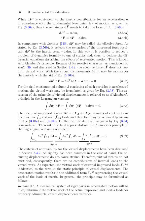
36 3 Fundamental Considerations
When dF ∗ is equivalent to the inertia contributions for an acceleration ain accordance with the fundamental Newtonian law of motion, as given byEq. (3.56a), then the remainder dF needs to take the form of Eq. (3.56b):
dF ∗ = a dm, (3.56a)dF = dF − a dm. (3.56b)
In compliance with Lanczos [118], dF may be called the effective force. Asstated by Eq. (3.56b), it reflects the extension of the impressed force resul-tant dF by the inertia term −a dm. In this way it is possible to reduce aproblem of dynamics formally to one of statics and, thus, to deduce the dif-ferential equations describing the effects of accelerated motion. This is knownas d’Alembert’s principle. Because of its reactive character, as mentioned byBudo [39] and discussed in Section 3.4.2, the effective force dF does not per-form virtual work. With the virtual displacements δu, it may be written forthe particle with the aid of Eq. (3.56b):
δuT dF = δuT (dF − a dm) = 0. (3.57)
For the rigid continuum of volume Λ consisting of such particles in acceleratedmotion, the virtual work may be formulated as given by Eq. (3.58). This ex-tension of the principle of virtual displacements is referred to as d’Alembert’sprinciple in the Lagrangian version:
∫
Λ
δuT dF =∫
Λ
δuT (dF − a dm) = 0. (3.58)
The result of impressed forces dF = dF Λ + dF ∂Λ consists of contributionsfrom volume fΛ and area f∂Λ loads and therefore may be replaced by meansof Eqs. (3.10a) and (3.10b). Further on, the density ρ as given by Eq. (3.54)is introduced. Therewith the final representation of d’Alembert’s principle inthe Lagrangian version is obtained:
∫
∂Λσ
δuT f∂Λ dA+∫
Λ
δuT fΛ dV︸ ︷︷ ︸
δV md
−∫
Λ
δuT aρdV︸ ︷︷ ︸
δV dl
= 0. (3.59)
The criteria of admissibility for the virtual displacements have been discussedin Section 3.4.2. As rigidity has been assumed in the case at hand, the oc-curring displacements do not cause strains. Therefore, virtual strains do notexist and, consequently, there are no contributions of internal loads to thevirtual work. As expected, the virtual work of external impressed loads δV md
is identical to the term in the static principle of virtual displacements. Theaccelerated motion results in the additional term δV dl representing the virtualwork of the loads of inertia. In general, the principle may be formulated asfollows:
Remark 3.5. A mechanical system of rigid parts in accelerated motion will bein equilibrium if the virtual work of the actual impressed and inertia loads forarbitrary admissible virtual displacements vanishes.

3.4 Principle of Virtual Work 37
3.4.6 Summation of Virtual Work Contributions
In Sections 3.4.2 and 3.4.5, the virtual work contributions of a mechanicalsystem being either static and deformable or dynamic and rigid were derived.They can be combined to picture a deformable dynamic system with the termsof Eqs. (3.45) and (3.59) as follows:
δV md + δV dl = δU md, (3.60a)∫
∂Λσ
δuT f∂Λ dA+∫
Λ
δuT (fΛ − aρ) dV =∫
Λ
δεT σ dV. (3.60b)
Alternatively, this formulation may be deduced starting from the interior con-servation of momentum, Eq. (3.61), which upgrades the interior mechanicalequilibrium, Eq. (3.14), with the inertia contributions of d’Alembert’s prin-ciple, Eq. (3.56b). Thereby the derivation steps can be transferred from Sec-tion 3.4.2.
�σ + fΛ − aρ = 0 in Λ. (3.61)The electric contributions from the principle of virtual potential, as derived inSection 3.4.4 and given by Eq. (3.53), still have to be incorporated. This canbe achieved equivalently by the addition or subtraction of Eqs. (3.60b) and(3.53). In conformance with Allik and Hughes [4] and in view of the symmetryproperties of the not yet introduced constitutive relation, the electrostaticexpressions will be subtracted from the mechanical ones. The virtual work ofexternal contributions takes the following form:
δV = δV md + δV dl − δV ep
=∫
∂Λσ
δuT f∂Λ dA+∫
Λ
(δuT
(fΛ − aρ
)− δϕqΛ
)dV −
∫
∂ΛD
δϕq∂Λ dA
=∫
∂Λ
{δuT −δϕ
}{
f∂Λ
q∂Λ
}
dA+∫
Λ
{δuT −δϕ
}{
fΛ − aρqΛ
}
dV.
(3.62)
Since the forces f∂Λ and charges q∂Λ on the boundary are zero apart fromtheir respective working surface, the surface integrals may be summarized.Then the integrands can be collated in vector form, as shown in the last line.Similarly, the virtual work of internal contributions can be formulated, wherethe vectors of virtual strains δεT and virtual electric field strength δET , aswell as the vectors of actual stresses σ and actual electric flux density D, canbe merged:
δU = δU md − δU ep
=∫
Λ
δεT σ dV −∫
Λ
δET D dV
=∫
Λ
{
δεT δET}{
σD
}
dV. (3.63)
Here the negative sign has been incorporated into the representation of theelectric field strength by setting E = −E.

38 3 Fundamental Considerations
3.5 Other Variational Principles
The principle of virtual work is suitable for solving a wide range of problems.There are tasks however where different but related formulations might bemore useful. Thus, two prominent variational principles will be extended hereto take into account materials with electromechanical couplings. This novelapproach to Dirichlet’s principle of minimum potential energy will be em-ployed later in Section 6.3.2. In comparison to the principle of virtual work,the extended general Hamilton’s principle is considered to be equivalent andeven more versatile, but only its derivation will be demonstrated here.
3.5.1 Extended Dirichlet’s Principle of Minimum Potential Energy
Another important principle of mechanics, see Dym and Shames [70] or Sokol-nikoff [166] for details, will be extended here to electromechanically coupledproblems. Let there be a function U0 to establish the following relation be-tween the fields of mechanical stress σ and electric flux density D on the onehand, and the fields of mechanical strain ε and, for reasons to be clarified inSection 4.4.4, negative electric field strength E on the other:
{σD
}
=∂U0
∂{ ε
E
} =
{∂U0∂ε
∂U0
∂E
}
. (3.64)
Such a function U0 can be shown to exist for conservative systems with theirreversible processes, see Dym and Shames [70]. Thus, unlike the principleof virtual work derived above, the subsequent examination is limited to cer-tain material properties. For mechanical fields, the demand for reversibilityimplies elastic material behavior, linear as well as non-linear. Hence, in theaccustomed representations restricted to mechanical fields, the function U0 iscalled the elastic potential or strain energy density. In anticipation of subse-quent chapters, it needs to be stated here that mechanical behavior as wellas electromechanical coupling and electrostatic behavior of the consideredpiezoelectric materials is conservative as long as repolarization is avoided, seeFigure 4.1. The function U0 will be determined and analyzed in Section 4.4.4using the then available constitutive relation. For the extended examinationat hand, the function U0 may be described as electroelastic energy density;sometimes it is termed electric enthalpy density, see Tichy and Gautschi [174].Consequently, integration over the entire structure results in the electroelasticenergy
U =∫
Λ
U0 dV. (3.65)
In the virtual work of internal contributions given by Eq. (3.63), the fieldquantities appearing in virtual and actual form are in no way connected.With the substitution of Eq. (3.64) into Eq. (3.63), this independence from

3.5 Other Variational Principles 39
the material behavior is abolished:
δU =∫
Λ
{
δεT δET} ∂U0
∂{ ε
E
} dV = δ∫
Λ
U0 dV. (3.66)
In the static portions of the virtual work of external contributions, the forcesand charges acting on the constant volume and surface of the structure arenot altered by the arbitrary variations δu of displacements and δϕ of electricpotential respectively. Thus, the left-hand sides of Eqs. (3.45) and (3.53) maybe written in the following form:
δV md = δ(∫
∂Λσ
uT f∂Λ dA+∫
Λ
uT fΛ dV)
, (3.67a)
δV ep = δ(∫
∂ΛD
ϕq∂Λ dA+∫
Λ
ϕqΛ dV)
. (3.67b)
Equations (3.66) and (3.67) change the principle of virtual work of Eq. (3.41)to the following representation:
δ(
U − V md + V ep)
= 0. (3.68)
To satisfy this statement, the expression in parentheses describing the poten-tial energy is required to assume a stationary value. Furthermore, it can beshown that this extremum has to be the minimum of the potential energy,see Sokolnikoff [167] or Knothe and Wessels [113]. Thus, Dirichlet’s principleof minimum potential energy can be extended to electromechanically coupledmaterials:
Remark 3.6. A uniform electromechanically coupled system will be in equilib-rium for the set of displacements and electric potential satisfying the boundaryconditions that produces the absolute minimum of potential energy.
U − V md + V ep ⇒ min. (3.69)
3.5.2 Extended General Hamilton’s Principle
D’Alembert’s principle in the Lagrangian version, as derived in Section 3.4.5,uses infinitesimal virtual displacements about the instantaneous system state.For this reason, it is referred to as a differential principle. When infinitesimalvirtual deviations from the entire motion of a system between two instants intime are examined, then it is an integral principle like Hamilton’s principle, seeGoldstein [86], Sokolnikoff [167], Szabo [172] or Morgenstern and Szabo [126].Here the derivation from the prior to the latter principle will be demonstrated,starting with conversion of the virtual work of the inertia loads δV dl, includedin Eq. (3.59). With Eq. (3.54) and acceleration as derivative of velocity, it

40 3 Fundamental Considerations
may be split as follows:
δV dl = −∫
Λ
δuT a dm with a =dv
dt
= −∫
Λ
δuT dv
dtdm = − d
dt
∫
Λ
δuT v dm+∫
Λ
ddtδuT v dm. (3.70)
The last term, with the aid of Schwarz’s theorem stating the possibility tointerchange the order of taking partial derivatives and velocity as derivativeof displacement, can be shown to represent the virtual change of kinetic en-ergy V ke:
δV ke =∫
Λ
ddtδuT v dm with
ddtδuT = δ
duT
dt= δvT
=∫
Λ
δvT v dm = δ12
∫
Λ
|v|2 dm. (3.71)
Application of Eq. (3.71) to (3.70) leads to Lagrange’s central equation:
δV dl = − ddt
∫
Λ
δuT v dm+ δV ke. (3.72)
With its substitution into d’Alembert’s principle in the Lagrangian version ofEq. (3.59), one obtains Eq. (3.73). Integration over the period of time from t0to t1, where the virtual displacements are zero by definition at these end pointssuch that δu (t0) = δu (t1) = 0, leads to the general Hamilton’s principle ofEq. (3.74):
δV md + δV ke =ddt
∫
Λ
δuT v dm, (3.73)∫ t1
t0
(δV md + δV ke
)dt = 0. (3.74)
Instead of using d’Alembert’s principle in the Lagrangian version, Lagrange’scentral equation, Eq. (3.72), may be substituted into the complete principleof virtual work, Eq. (3.41) with (3.62) and (3.63). After the intermediate stepof Eq. (3.75), this finally leads to the general Hamilton’s principle with anextension to deformable piezoelectric bodies of Eq. (3.76):
δV md − δV ep + δV ke − δU md + δU ep =ddt
∫
Λ
δuT v dm, (3.75)∫ t1
t0
(δV md − δV ep + δV ke − δU md + δU ep) dt = 0. (3.76)

4
Piezoelectric Materials
As pointed out in the introductory chapter, there are many multifunctionalmaterials that can be applied to realize adaptive structural systems. Theyare distinguished by means of excitation mechanism, application range, andmaturity of development. While research in material science will widen thechoice in the future, currently only piezoelectric materials are suitable forthe intended purpose. Therefore, the piezoelectric effect and its constitutivedescription is examined in detail in this chapter.
4.1 Piezoelectric Effect
Piezoelectricity represents the interdependence between mechanical and elec-trostatic fields, which is approximately proportional for the majority of ap-plications. The direct piezoelectric effect describes the electrostatic reactionto a mechanical load, while the converse piezoelectric effect describes the me-chanical reaction to an electrostatic load. Thorough portrayals of the physicalbackground are given by Cady [41], Ikeda [103], Tichy and Gautschi [174]as well as application oriented presentations by Chopra [53], Janocha [106],Elspass and Flemming [72].
4.1.1 Historical Development
According to Cady [41], tourmaline crystals came from Ceylon to Europein the early 18th century and were found to possess a number of remark-able characteristics. Although a relationship between mechanical and elec-trical behavior had been expected by the scientific community, it could notbe demonstrated experimentally for many years. Finally in 1880, the broth-ers Pierre and Jacques Curie [59,60] discovered the proportionality of pres-sure applied in specific directions and electric charges appearing with op-posed signs on opposed surfaces. The following year, the term piezoelectriceffect has been proposed for the observed behavior by Hankel [91]. The prefix
T.H. Brockmann, Theory of Adaptive Fiber Composites,Solid Mechanics and Its Applications 161,c© Springer Science + Business Media B.V. 2009

42 4 Piezoelectric Materials
“piezo” is derived from the Greek verb “πιεζω” meaning to press or squeeze.The Curie brother also experimentally demonstrated the existence of theconverse piezoelectric effect. Since then, other naturally occurring monocrys-talline piezoelectric materials have been examined, the most important beingquartz. Significant impetus has been generated by the discovery of piezo-electricity in polycrystalline ceramic materials like barium-titanate (BT) inthe 1940’s and lead-zirconate-titanate (PZT) in the 1950’s; the latter stilldominates transducer applications. Semicrystalline piezoelectric polymers onthe basis of polyvinylidenefluoride (PVDF) usually in the form of thin filmshave been available since the late 1960’s. Newer development tendencies aredirected towards the improvement of PZT ceramics by doping them withadditional components or producing artificial piezoelectric monocrystals, seeNelson et al. [131].
4.1.2 Crystal Structures
The piezoelectric effect is associated with the existence of an electric dipole inthe elementary cell of the crystal structure. Such an electric dipole representspositive and negative charges with non-coinciding centers of concentration.The polar axis describes the dipole orientation with the polar direction fromthe negative to the positive center. Charge quantity and center-to-center spac-ing define the dipole moment. Relating the latter to the associated volumecharacterizes the polarization. An electric dipole and thus polarization canexist only when the elementary cell is not symmetric with respect to a pointreferred to as the inversion center, see Giacovazzo [83]. So the piezoelectriceffect occurs only in such non-centrosymmetric crystals.
Polar Crystals and Polar-Neutral Crystals
The non-centrosymmetric crystals may be divided into two groups with re-spect to the occurrence of polar directions, see Tichy and Gautschi [174] orMoulson and Herbert [128]. When all dipoles are aligned with a unique polardirection, the crystals possess a spontaneous polarization and are denominatedas polar crystals. The change of this existing polarization due to mechanicalimplications leads to the piezoelectric effect. Thermal influences may alsochange the spontaneous polarization of polar crystals; the resulting behavioris called the pyroelectric effect. In the case of non-unique polar directions,a neutralization occurs and prevents a spontaneous polarization. Therefore,such crystals are called polar-neutral crystals. Here the deformation causesa modification of the crystal symmetry, such that a unique polar directionemerges and the crystal becomes polarized along this direction. Thus, thepolar-neutral crystals exhibit the piezoelectric effect but not the pyroelectriceffect.

4.1 Piezoelectric Effect 43
Ferroelectric Polar Crystals
There is an important subgroup of the polar crystals which possesses the abil-ity to change the spontaneous polarization in reaction to electrostatic fieldsto another stable orientation, respectively, to a reverse configuration. Due tothe analogy to ferromagnetic behavior, the name ferroelectricity has been in-troduced. Corresponding to the magnetic domains associated with the nameof Pierre-Ernest Weiss, domains of largely uniform dipole orientations developin the process of minimization of the free energy. These domains cause thenon-linear properties of ferroelectric materials, especially with respect to theelectrostatic polarization resulting in a hysteresis curve in alternating fields,Figure 4.1(a). In general, the polarization is also associated with a change inmaterial properties and shape due to the implied modifications of the crystalstructure. Therefore, the existence of a residual polarization in ferroelectricmaterials consequently leads to a lasting deformation, Figure 4.1(b). As repo-
Fig. 4.1. Qualitative representation of hysteresis loops of PZT material; (a) polar-ization P and (b) strain ε as functions of the applied electric field strength E.

44 4 Piezoelectric Materials
larization reduces the life span of ferroelectric material, it is usually polarizedonce and then operated within subcritical field levels. For PZT materials, thisoften is an electric field strength in the range between −0.5 and 1.5 kV·mm−1.As shown in Figure 4.1(b), the electromechanical coupling is still not fully lin-ear within this range. Details on the matters of hysteretic behavior and non-linear coupling are provided, for example, by Kamlah [109] and Zhou [187].Another ferroelectric characteristic is the limitation of the spontaneous po-larization state to a certain temperature range. Above a critical temperature,called the Curie temperature, there is a phase change to a centrosymmetriccrystal class, and the piezoelectric effect vanishes.
Monocrystalline Examples
The monocrystalline seignette salt NaKC4H4O6·H2O was the first found tobelong to the group of ferroelectric polar crystals, while aluminum-boron-silicate (Na,Ca)(Mg,Fe)3B3Al6Si6(O,OH,F)31, known as tourmaline, is anexample of a non-ferroelectric polar crystal. Siliciumdioxide or quartz SiO2
below a temperature of 573◦C is a typical representative of a polar-neutralcrystal. Recent developments in material science are concerned with ferro-electric single crystal systems like (1 − x)Pb(Mg1/3Nb2/3)O3−x PbTiO3 or(1 − x)Pb(Zn1/3Nb2/3)O3−x PbTiO3, where x indicates the share of lead-titanate. These materials with the abbreviations PMN-PT and PZN-PT havevery competitive electromechanical properties.
Polycrystalline Characteristics
While monocrystals are characterized by a continuous spatial arrangementof elementary cells, polycrystals consist of a multitude of crystalline grains,so-called crystallites, with alike properties inside their boundaries but chang-ing orientations across the boundaries. A regular spatial pattern of orientedcrystallites is called texture. In order to exhibit the piezoelectric effect, suchtextures also must not possess an inversion center, otherwise, even when thecrystallites are piezoelectric, the effect would be neutralized. Piezoelectric ce-ramics are a typical example of polycrystalline materials. Most prominent withrespect to a broad application are barium-titanate BaTiO3 and particularlylead-zirconate-titanate Pb(Zr,Ti)O3. The structure of both materials may besummarized by the general formula A2+B4+O2−
3 . With respect to their ferro-electric nature, they switch from the non-centrosymmetric tetragonal crystalclass to the centrosymmetric cubic crystal class when their respective Curietemperature is exceeded and thus loose their piezoelectric properties. Bothconfigurations are shown in Figure 4.2 with the decisive asymmetric disloca-tion of the B4+ component.

4.2 Constitutive Formulation 45
Fig. 4.2. Elementary crystal cell; (a) cubic configuration and (b) tetragonal config-uration due to polarization along the e3-direction.
Semicrystalline Characteristics
Semicrystalline polymers are thermoplastics and consist of crystallites sur-rounded by a transitional phase which again is embedded into an amor-phous phase. Polyvinylidenefluoride is such a material with piezoelectric prop-erties. Its long molecular chains, typical for a polymer, may be found indifferent configurations of spatial arrangement with a polar and a polar-neutral crystal structure for each of these configurations. Subjected to ther-mal, mechanical, and electrostatic influences, the properties may be alteredsignificantly. The reaction on electrostatic influences points to the ferroelec-tric nature of semicrystalline polymers. Details are given, for example, byElspass and Flemming [72].
4.2 Constitutive Formulation
The fundamental considerations of Chapter 3 are independent of the proper-ties of the materials and therefore are not sufficient to describe the behaviorof the mechanical or electrostatic system. The missing links are the consti-tutive relations between stresses and strains on the mechanical side, betweenflux density and field strength on the electrostatic side, and the connectionbetween the mechanical and electrostatic side. Effects like piezoelectricity cou-ple the mechanical and electrostatic fields. For the subsequent considerationsidentical material properties at every location of the continuum can be pre-sumed due to its macroscopic homogeneity.

46 4 Piezoelectric Materials
4.2.1 Mechanical Fields
We limit our examination to materials with a unique coherence between thepresent local stress and strain states, where deformation history or time-dependent processes do not matter. Under these conditions, the removal ofloads leads to a complete reversal of deformations. In addition, we demandindependence from mechanical field intensities within the intensity levels ofinterest:
Remark 4.1. The mechanical behavior of the materials will be assumed to beelastic and linear.
The Cauchy stress tensor σ and Green Lagrange strain tensor εGL are ofsecond order and may be connected for a general anisotropic linear elasticmaterial via a fourth-order tensor. The originally 81 constants of such anelasticity tensor reduce to 36 due to the symmetry of the stress and straintensor, and may be represented by a square matrix of dimension six. Becauseof the potential property of elastic materials, such a matrix is symmetric andthus the number of independent components is further reduced to 21. Forsmall displacements, the mechanical constitutive relation with the stiffnessmatrix C or with the compliance matrix S reads
σ = Cε or ε = Sσ with S = C−1. (4.1)
Technically relevant applications are hardly concerned with complete aniso-tropy. Composites with a regular distribution of constituents along the princi-pal axes are an example of a material with three orthogonal planes of symme-try. The description of such orthotropic properties requires nine independentmatrix entries:
⎧⎪⎪⎪⎪⎪⎪⎨
⎪⎪⎪⎪⎪⎪⎩
σ1
σ2
σ3
τ23τ31τ12
⎫⎪⎪⎪⎪⎪⎪⎬
⎪⎪⎪⎪⎪⎪⎭
=
⎡
⎢⎢⎢⎢⎢⎢⎣
C11 C12 C13 0 0 0C12 C22 C23 0 0 0C13 C23 C33 0 0 00 0 0 C44 0 00 0 0 0 C55 00 0 0 0 0 C66
⎤
⎥⎥⎥⎥⎥⎥⎦
⎧⎪⎪⎪⎪⎪⎪⎨
⎪⎪⎪⎪⎪⎪⎩
ε1ε2ε3γ23γ31γ12
⎫⎪⎪⎪⎪⎪⎪⎬
⎪⎪⎪⎪⎪⎪⎭
. (4.2)
Composites with uniformly distributed unidirectional fibers aligned with aprincipal axis additionally possess a plane of isotropy in the transverse direc-tion, where the material behavior is invariant to rotations. For such trans-versely isotropic properties, the number of constants is reduced to five. Whenthe concerned axis of rotation is oriented in the e3-direction,
C22 = C11, C23 = C13, C55 = C44, C66 =12
(C11 − C12) . (4.3)

4.2 Constitutive Formulation 47
If every arbitrary section plane is a plane of isotropy, the material is isotropic;there only two independent constants remain:
C33 = C22 = C11, C23 = C13 = C12,
C44 = C55 = C66 =12(C11 − C12).
(4.4)
4.2.2 Electrostatic Fields
Presuming that there is no electrostatic equivalent to mechanical inelasticity,compare with Remark 4.1, the essential demand concerning the properties ofdielectric materials is independence of the electrostatic field intensities withinthe intensity levels of interest:
Remark 4.2. The electrostatic behavior of the materials will be assumed to belinear.
The electric flux density D and electric field strength E are vectors, i.e.tensors of first order and therefore may be related via a tensor of second orderwith nine constants for the three dimensions. Due to the potential propertyalso observed for electrostatic fields, the tensor is symmetric and thus con-tains six independent entries. The electrostatic constitutive relation can beexpressed with the aid of the dielectric permittivity matrix ε (to be distin-guished from the strains ε) or its inverse β:
D = εE or E = βD with β = ε−1. (4.5)
Thereby these specifications occasionally are given relative to the dielectricpermittivity of vacuum ε0:
ε = εε0 with ε0 = 8.855 × 10⁻¹² AsVm
. (4.6)
The rhombic crystal class as well as composites with adequate constituentsand layout, for instance, possess orthotropic properties in analogy to the me-chanical material properties. Therefore, only the three entries on the diagonalof the constitutive matrix are retained:
⎧⎨
⎩
D1
D2
D3
⎫⎬
⎭=
⎡
⎣ε11 0 00 ε22 00 0 ε33
⎤
⎦
⎧⎨
⎩
E1
E2
E3
⎫⎬
⎭. (4.7)
Transversely isotropic properties, as exhibited, for example, by the tetragonalcrystal class, require two dielectric constants and thus using the distinct axisagain in the e3-direction this implies
ε22 = ε11. (4.8)
For isotropic properties, as exhibited for example by the cubic crystal class,there is only one dielectric constant:
ε33 = ε22 = ε11. (4.9)
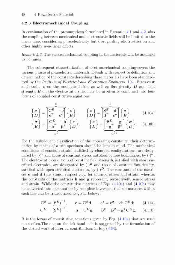
48 4 Piezoelectric Materials
4.2.3 Electromechanical Coupling
In continuation of the presumptions formulated in Remarks 4.1 and 4.2, alsothe coupling between mechanical and electrostatic fields will be limited to thelinear case, considering piezoelectricity but disregarding electrostriction andother highly non-linear effects.
Remark 4.3. The electromechanical coupling in the materials will be assumedto be linear.
The subsequent characterization of electromechanical coupling covers thevarious classes of piezoelectric materials. Details with respect to definition anddetermination of the constants describing these materials have been standard-ized by the Institute of Electrical and Electronics Engineers [104]. Stresses σand strains ε on the mechanical side, as well as flux density D and fieldstrength E on the electrostatic side, may be arbitrarily combined into fourforms of coupled constitutive equations:
{σD
}
=
C︷ ︸︸ ︷[CE −eeT εε
]{εE
}
,{
εD
}
=
S︷ ︸︸ ︷[SE ddT εσ
]{σE
}
, (4.10a){
σE
}
=[CD −h
−hT βε
]
︸ ︷︷ ︸S−1
{εD
}
,{
εE
}
=[
SD g−gT β
σ
]
︸ ︷︷ ︸C−1
{σD
}
. (4.10b)
For the subsequent classification of the appearing constants, their determi-nation by means of a test specimen should be kept in mind. The mechanicalconditions of constant strain, satisfied by clamped configurations, are desig-nated by (·)ε and those of constant stress, satisfied by free boundaries, by (·)σ.The electrostatic conditions of constant field strength, satisfied with short cir-cuited electrodes, are designated by (·)E and those of constant flux density,satisfied with open circuited electrodes, by (·)D. The constants of the matri-ces e and d thus stand, respectively, for induced stress and strain, whereasthe constants of the matrices h and g represent, respectively, sensed stressand strain. While the constitutive matrices of Eqs. (4.10a) and (4.10b) maybe converted into one another by complete inversion, the sub-matrices withineach line can be transformed as given below:
CE =(SE
)−1, e = CEd, εε = εσ − dT CEd; (4.11a)
CD =(SD
)−1, h = CDg, β
ε = βσ + gT CDg. (4.11b)
It is the forms of constitutive equations given by Eqs. (4.10a) that are usedmost often.The one on the left-hand side is suggested by the formulation ofthe virtual work of internal contributions in Eq. (3.63).

4.2 Constitutive Formulation 49
4.2.4 Spatial Rotation
The mechanical constitutive relations of Eqs. (4.1) are set up with respect tothe orthonormal base vectors e1, e2, e3, which usually represent the principalaxes of the material. When a material description in rotated coordinates withthe orthonormal base vectors es, en, ex is necessary, this can be achieved withthe aid of the transformation relations of Eqs. (3.27) and (3.28) as follows:
σ (s, n, x) = TCTT ε (s, n, x) , (4.12)
ε (s, n, x) =(T−1
)TST−1σ (s, n, x) . (4.13)
As the electrodes necessary to capture the electrostatic fields are generally at-tached with respect to the associated principal axes, they follow the rotationand thus the electrostatic fields do not undergo the transformation. Never-theless, their interaction with the mechanical fields via the electromechanicalcoupling coefficients needs to be taken into account. This is accomplishedby extending the mechanical transformation matrix T with the identity ma-trix I for the transformation of the electromechanical constitutive relation ofEqs. (4.10). For the variant on the left-hand side of Eq. (4.10a), this means
{σ (s, n, x)D (1, 2, 3)
}
=[T
I
]
︸ ︷︷ ︸T
[CE −eeT εε
]
︸ ︷︷ ︸C
[T
I
]T
︸ ︷︷ ︸TT
{ε (s, n, x)E (1, 2, 3)
}
. (4.14)
When the multiplication is executed for the sub-matrices, it can be recognizedthat the transformation behavior of the mechanical stiffness coefficients givenby Eq. (4.12) is reproduced in the upper left part, and the unchanged dielectricpermittivity coefficients remain in the lower right part of the resulting matrix.As expected, the electromechanical coupling coefficients to be found off thediagonal are transformed, preserving their properties of being transposed andnegated to each other:
TCTT =
[TCETT −TeeT TT εε
]
. (4.15)
4.2.5 Analogy of Electrically and Thermally Induced Deformations
The simulation of component parts exhibiting electromechanical coupling withthe aid of commercial finite element packages is subject to some restrictions.Usually the piezoelectric effect is considered only in connection with volumeelements, see Freed and Babuska [76]. For complex structures, the modelingwith volume elements often does not represent a viable procedure with respectto implementation and calculation expenditure. A prominent example for thisare structures with thin walls made of multiple layers. Their mechanical be-havior may be simulated efficiently with layered structural shell elements,
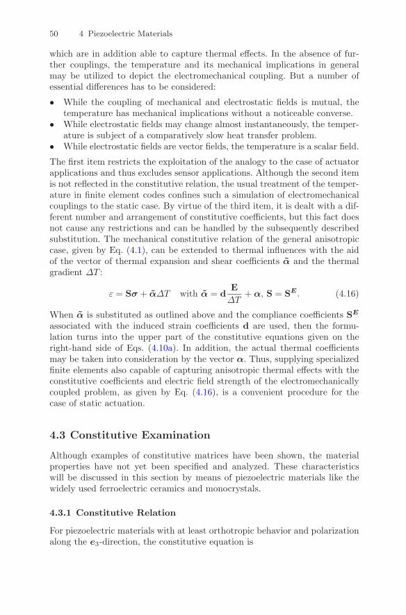
50 4 Piezoelectric Materials
which are in addition able to capture thermal effects. In the absence of fur-ther couplings, the temperature and its mechanical implications in generalmay be utilized to depict the electromechanical coupling. But a number ofessential differences has to be considered:
• While the coupling of mechanical and electrostatic fields is mutual, thetemperature has mechanical implications without a noticeable converse.
• While electrostatic fields may change almost instantaneously, the temper-ature is subject of a comparatively slow heat transfer problem.
• While electrostatic fields are vector fields, the temperature is a scalar field.
The first item restricts the exploitation of the analogy to the case of actuatorapplications and thus excludes sensor applications. Although the second itemis not reflected in the constitutive relation, the usual treatment of the temper-ature in finite element codes confines such a simulation of electromechanicalcouplings to the static case. By virtue of the third item, it is dealt with a dif-ferent number and arrangement of constitutive coefficients, but this fact doesnot cause any restrictions and can be handled by the subsequently describedsubstitution. The mechanical constitutive relation of the general anisotropiccase, given by Eq. (4.1), can be extended to thermal influences with the aidof the vector of thermal expansion and shear coefficients α and the thermalgradient ΔT :
ε = Sσ + αΔT with α = dEΔT
+ α, S = SE . (4.16)
When α is substituted as outlined above and the compliance coefficients SE
associated with the induced strain coefficients d are used, then the formu-lation turns into the upper part of the constitutive equations given on theright-hand side of Eqs. (4.10a). In addition, the actual thermal coefficientsmay be taken into consideration by the vector α. Thus, supplying specializedfinite elements also capable of capturing anisotropic thermal effects with theconstitutive coefficients and electric field strength of the electromechanicallycoupled problem, as given by Eq. (4.16), is a convenient procedure for thecase of static actuation.
4.3 Constitutive Examination
Although examples of constitutive matrices have been shown, the materialproperties have not yet been specified and analyzed. These characteristicswill be discussed in this section by means of piezoelectric materials like thewidely used ferroelectric ceramics and monocrystals.
4.3.1 Constitutive Relation
For piezoelectric materials with at least orthotropic behavior and polarizationalong the e3-direction, the constitutive equation is

4.3 Constitutive Examination 51
⎧⎪⎪⎪⎪⎪⎪⎪⎪⎪⎪⎪⎪⎨
⎪⎪⎪⎪⎪⎪⎪⎪⎪⎪⎪⎪⎩
σ1
σ2
σ3
τ23τ31τ12D1
D2
D3
⎫⎪⎪⎪⎪⎪⎪⎪⎪⎪⎪⎪⎪⎬
⎪⎪⎪⎪⎪⎪⎪⎪⎪⎪⎪⎪⎭
=
⎡
⎢⎢⎢⎢⎢⎢⎢⎢⎢⎢⎢⎢⎣
CE11 CE
12 CE13 0 0 0 0 0 −e31
CE12 CE
22 CE23 0 0 0 0 0 −e32
CE13 CE
23 CE33 0 0 0 0 0 −e33
0 0 0 CE44 0 0 0 −e24 0
0 0 0 0 CE55 0 −e15 0 0
0 0 0 0 0 CE66 0 0 0
0 0 0 0 e15 0 εε11 0 00 0 0 e24 0 0 0 εε22 0e31 e32 e33 0 0 0 0 0 εε33
⎤
⎥⎥⎥⎥⎥⎥⎥⎥⎥⎥⎥⎥⎦
⎧⎪⎪⎪⎪⎪⎪⎪⎪⎪⎪⎪⎪⎨
⎪⎪⎪⎪⎪⎪⎪⎪⎪⎪⎪⎪⎩
ε1ε2ε3γ23γ31γ12E1
E2
E3
⎫⎪⎪⎪⎪⎪⎪⎪⎪⎪⎪⎪⎪⎬
⎪⎪⎪⎪⎪⎪⎪⎪⎪⎪⎪⎪⎭
.
(4.17)Together with the mechanical and electrostatic simplifications introduced byEqs. (4.3) and (4.8), transversely isotropic properties can be characterized forthe piezoelectric coupling by
e32 = e31, e15 = e24. (4.18)
It should be mentioned that the otherwise transversely isotropic properties ofthe typical piezoelectric materials, given by Table A.3 in the Appendix, showdeviations of a different degree from the last relation of Eqs. (4.3) expressingthe dependence of CE
66. While these deviations are relatively small in the caseof the PZT ceramics, the properties of PMN-PT single crystals do not complywith this condition at all.
Partial Coupling
In the structure of the constitutive equation for the mechanically and electro-statically orthotropic piezoelectric material of Eq. (4.17), the partial couplingneeds to be noted. The normal stresses and strains in all three directionsare solely connected to flux density and field strength along the polarizationdirection: ⎧
⎪⎪⎨
⎪⎪⎩
σ1
σ2
σ3
D3
⎫⎪⎪⎬
⎪⎪⎭
=
⎡
⎢⎢⎣
CE11 CE
12 CE13 −e31
CE12 CE
22 CE23 −e32
CE13 CE
23 CE33 −e33
e31 e32 e33 εε33
⎤
⎥⎥⎦
︸ ︷︷ ︸E
⎧⎪⎪⎨
⎪⎪⎩
ε1ε2ε3E3
⎫⎪⎪⎬
⎪⎪⎭
. (4.19)
The shear stresses and strains in the planes between polarization and trans-verse directions are coupled to flux density and field strength along the re-spective transverse axis:
{τ31D1
}
=[CE
55 −e15e15 εε11
]
︸ ︷︷ ︸G1
{γ31E1
}
and{τ23D2
}
=[CE
44 −e24e24 εε22
]
︸ ︷︷ ︸G2
{γ23E2
}
.
(4.20)Complete decoupling is found in the case of shear in the plane transverse tothe polarization direction:
τ12 = CE66γ12. (4.21)

52 4 Piezoelectric Materials
4.3.2 Converse Piezoelectric Effect
To illustrate the behavior of piezoelectric material, the constitutive equationsof the previous subsection will be observed in further detail by means of a cubeof such matter. The principal axes of the polarized macroscopically homoge-neous material are aligned with the edges of the cube. For actuator applica-tions use is made of the converse piezoelectric effect, and thus the cube has tobe subjected to electrostatic fields. This is usually accomplished by supplyinga pair of electrodes in the form of opposed conductive surfaces with opposedelectric charges. This electric potential difference, together with the distancebetween the electrodes, leads to an associated electric field strength compo-nent according to Eq. (3.40). The aligned electric flux density component maybe determined via the dielectric permittivities, lower third of Eq. (4.17), whilethe field strength and flux density components in all other directions are zero.Depending on the mechanical boundary conditions applied to the cube, ei-ther strains in the free configuration or stresses in the clamped configurationare induced. For electrostatic fields opposed or transverse to the polarizationdirection, the field levels are limited by the risk of repolarization.
Normal Mode Actuation
Electrostatic field components in parallel with the polarization direction in-duce normal mode actuation, see Eq. (4.19). Not visible in the constitutiveequation, but explainable by a behavior corresponding to Poisson’s effect in-cluded in the piezoelectric constants, the signs of strains or stresses paralleland transverse to the applied electrostatic fields are opposed. The deforma-tion of a piezoelectric cube subjected to electrostatic fields in the direction ofpolarization is shown in Figure 4.3.
Fig. 4.3. Normal mode of the converse piezoelectric effect.
Shear Mode Actuation
Electrostatic field components transverse to the direction of polarization in-duce shear mode actuation, see Eq. (4.20). The particular shear strains or

4.3 Constitutive Examination 53
shear stresses appear in the plane unfolding between the direction of the ap-plied electrostatic field component and the polarization direction. The defor-mation of a piezoelectric cube subjected to electrostatic fields transverse tothe direction of polarization is shown in Figure 4.4.
Fig. 4.4. Shear mode of the converse piezoelectric effect.
4.3.3 Direct Piezoelectric Effect
For sensor applications, use is made of the direct piezoelectric effect and thusthe piezoelectric cube described above now has to be subjected to mechan-ical fields. Strains and stresses are applied via associated surfaces either byprescribed displacements in a clamped configuration or by applied forces in afree configuration. Besides the intended sensor application, this, of corrse, isalso relevant to the case of solely passive transmission of loads. Consequently,the subsequent examinations are also important for the general application ofelectromechanically coupled materials in adaptive structures. For mechanicalfields operating opposed or transverse to the polarization direction, the fieldlevels are limited by the risk of repolarization similar to the actuation case.
External Electric Influences
The electrostatic fields forming in a single direction as the result of basic loadcases depend on the electric boundary conditions and are thus influenced bythe electrode configuration. When the electrodes on the associated surfaces arenon-existent or disconnected, only the particular electric field strength compo-nent shows a constant non-zero distribution. The resulting electric potentialdifference with accumulating charges on the electrodes may be determinedby voltage measurement and is proportional to strain or stress, respectively.

54 4 Piezoelectric Materials
When the electrodes on the associated surfaces are connected, only the par-ticular electric flux density component shows a constant non-zero distributionwith opposed orientation. Charges cannot accumulate on the electrodes asthey flow off instantaneously. For a dynamic process, this flow of charges maybe determined by a current measurement, and is proportional to the strainrate, respectively stress rate. From the energetic point of view, the chargecompensation must also have consequences for the mechanical fields. Thisbecomes apparent by reorganization of the constitutive relation for these con-ditions and is reflected in the dissimilar stiffness and compliance matrices ofEqs. (4.10a) and (4.10b). These influences may be summarized for the basicload cases with resulting electrostatic fields in q-direction:
• Non-existent or disconnected electrodes→ Di = 0, Ei �=q = 0, Ei=q �= 0,
higher effective stiffness.• Connected electrodes
→ Ei = 0, Di �=q = 0, Di=q �= 0 (opposed orientation),lower effective stiffness.
These switchable properties may be used to tune the frequency response ofa structure, for example, when eigenfrequencies need to be avoided duringthe run-up of rotating machinery. Furthermore, the connection of electrodesvia resistors or inductors permits the damping or insulation of vibrations bypassive means.
Normal Mode Sensing
When a cube is subjected to normal strains or stresses in any of the threespatial directions, one of the electrostatic fields, contingent upon the electricboundary conditions, is induced parallel or anti-parallel to the polarizationdirection. Thus, without additional information, the directions of mechanicalstimulus cannot be distinguished by such a sensor. For the different cases ofelectric boundary conditions, the electrostatic fields developing in a piezoelec-tric cube subjected to normal loads are shown in Figure 4.5 together with thecorresponding deformations of the transversely isotropic material.
Shear Mode Sensing
When the cube is subjected to shear strains or stresses in the plane perpendic-ular to the polarization direction due to the non-existent coupling, no sensorsignal can be detected. In the remaining cases, a unique association of planeof shear and direction of electrostatic field is ensured as inversion of the ac-tuator behavior. For the different cases of electric boundary conditions, theelectrostatic fields developing in a piezoelectric cube subjected to shear loadsare shown together with the corresponding deformations in Figure 4.6.

4.3 Constitutive Examination 55
Fig. 4.5. Normal mode (surface loads F ) of the direct piezoelectric effect with non-existent or disconnected (E �= 0, D = 0; light colored state) or connected (D �= 0,E = 0; dark colored state) electrodes normal to the e3-direction.
Fig. 4.6. Shear mode (surface loads F ) of the direct piezoelectric effect with non-existent or disconnected (E �= 0, D = 0; light colored state) or connected (D �= 0,E = 0; dark colored state) electrodes (a) normal to the e2-direction and (b) normalto the e1-direction.

56 4 Piezoelectric Materials
Complications
For the considered uniform mechanical fields, the induced electrostatic fieldsobserved by means of the exemplary cube are also expected to be uniform.This holds true as long as the electrodes are appropriately mounted, thus per-pendicular to the electrostatic field. Things change significantly when othersurfaces are furnished with conductive elements; the previously immobile andunequal charges are now able to balance on such surfaces. This kind of dis-turbance has consequences for the electrostatic field and thus also for themechanical behavior. The linear electric potential distribution, correspondingto a constant e1-direction component of the electric field strength as a resultof pure shear load, is shown in Figure 4.7(a). The identical loading case, justwith provision for conductivity on the surfaces transverse to the e3-direction,and the resulting non-linear inhomogeneous electric potential distribution isdemonstrated in Figure 4.7(b). A noticeable decrease is observed, when thearising deformations are used to calculate the effective shear stiffness.
Fig. 4.7. Electric potential distribution in a piezoelectric cube subjected to shear inthe 3-1-plane (a) without electrodes (b) with connected or disconnected electrodestransverse to the e3-direction.
4.4 Constitutive Reduction
For the typical applications of piezoelectric materials, simplifying assumptionswith respect to the mechanical and electrostatic fields are reasonable. Thesemay be introduced in consequence of the spatial extent and electroding of theconsidered structure and, namely, are assumptions of planar mechanical andunidirectional electrostatic fields. Thereby, the variants of the latter, although
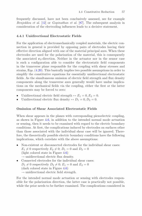
4.4 Constitutive Reduction 57
frequently discussed, have not been conclusively assessed, see for exampleBenjeddou et al. [12] or Gopinathan et al. [87]. The subsequent analysis inconsideration of the electroding influences leads to a decisive statement.
4.4.1 Unidirectional Electrostatic Fields
For the application of electromechanically coupled materials, the electric con-nection in general is provided by opposing pairs of electrodes having theireffective direction aligned with one of the material principal axes. When theseelectrodes are used for the polarization of the material, this is consequentlythe associated e3-direction. Neither in the actuator nor in the sensor caseis such a configuration able to consider the electrostatic field componentsin the transverse plane responsible for the coupling with shear stresses andstrains, Eqs. (4.20). This basically implies two possible assumptions in order tosimplify the constitutive equations for essentially unidirectional electrostaticfields. As the simultaneous omission of electric field strength and flux densitycomponents along the transverse axes generally would have undue implica-tions on the mechanical fields via the coupling, either the first or the lattercomponents may be forced to zero:
• Unidirectional electric field strength ↔ E1 = 0, E2 = 0.• Unidirectional electric flux density ↔ D1 = 0, D2 = 0.
Omission of Shear Associated Electrostatic Fields
When shear appears in the planes with corresponding piezoelectric coupling,as shown in Figure 4.6, in addition to the intended normal mode actuationor sensing, then it needs to be examined with regard to the electric boundaryconditions. At first, the complications induced by electrodes on surfaces otherthan those associated with the individual shear case will be ignored. There-fore, the theoretically possible electric boundary conditions have the followingimplications, which correlate with the above assumptions:
• Non-existent or disconnected electrodes for the individual shear cases:E1 �= 0 respectively E2 �= 0; D1 = 0 and D2 = 0(light colored state in Figure 4.6)→ unidirectional electric flux density.
• Connected electrodes for the individual shear cases:D1 �= 0 respectively D2 �= 0; E1 = 0 and E2 = 0(dark colored state in Figure 4.6)→ unidirectional electric field strength.
For the intended normal mode actuation or sensing with electrodes respon-sible for the polarization direction, the latter case is practically not possible,while the prior needs to be further examined. The complications considered in

58 4 Piezoelectric Materials
Fig. 4.8. Electric potential distribution due to shear in piezoelectric cuboids withelectrodes transverse to the e3-direction and with an aspect ratio (a) of l3/l1 = 4and (b) of l3/l1 = 1/2.
the previous subsection have to be taken into account. As illustrated by Fig-ure 4.7(b), the mismatched electroding disturbs the otherwise linear electricpotential distribution. But away from the electrodes this influence is fadingand, therefore, the relative distance of electrodes needs to be considered. Theresulting overall behavior ranges between the following extremes:
• Marginal penetration by the disturbance due to mismatched electroding:E1 �= 0, D1 ≈ 0, D2 = 0, respectively, E2 �= 0, D2 ≈ 0, D1 = 0(linear electric potential distribution in the center of Figure 4.8(a))� unidirectional electric flux density.
• Extensive penetration by the disturbance due to mismatched electroding:D1 �= 0, E1 ≈ 0, E2 = 0, respectively, D2 �= 0, E2 ≈ 0, E1 = 0(vanishing electric potential difference in the center of Figure 4.8(b))� unidirectional electric field strength.
Unidirectional Electric Field Strength
For unidirectional electric field strength confined to the component E3, thetransverse electric flux density components D1, D2 as well as shear stress

4.4 Constitutive Reduction 59
components τ31, τ23 only depend on the associated shear strains γ31, γ23, asillustrated by Eqs. (4.20):
E1 = 0 → D1 = e15γ31, τ31 = CE55γ31; (4.22a)
E2 = 0 → D2 = e24γ23, τ23 = CE44γ23. (4.22b)
The internal energy of an electrostatic system is represented by the productof the correlated field strength and flux density components, as exemplarilyderived for the virtual work of internal charges, Eq. (3.53). The shear straininduced flux density components D1 and D2, as given in Eq. (4.22), do notcontribute by virtue of the above assumption. Thus, the assumption of unidi-rectional electric field strength is equivalent to the neglect of shear associatedelectrostatic energy contributions.
Unidirectional Electric Flux Density
For the remaining case of unidirectional electric flux density confined to thecomponent D3, the transverse electric field strength components E1, E2 maybe expressed in terms of the shear strains γ31, γ23. Therewith E1 and E2 canbe eliminated from the constitutive equations by static condensation. Thus,this modification of Eqs. (4.20) represents a purely mechanical interactionwith strengthened shear stiffnesses as the result of the piezoelectric effect:
D1 = 0 → E1 = −e15εε11γ31 → τ31 =
(
CE55 +
(e15)2
εε11
)
γ31; (4.23a)
D2 = 0 → E2 = −e24εε22γ23 → τ23 =
(
CE44 +
(e24)2
εε22
)
γ23. (4.23b)
Thereby, from the energetic point of view again, the shear associated electro-static energy contributions, so to speak, are transferred to the elastic energy.
Summary of Unidirectional Electrostatic Fields
The implications of both discussed simplifications of the constitutive relationsmay be illustrated by summarizing all the shear cases. With the assumption ofunidirectional electric field strength for the stresses of Eqs. (4.22), respectively,unidirectional electric flux density for the stresses of Eqs. (4.23), whereby theadditional terms of the latter are furnished with the variables υ23 and υ31,and Eq. (4.21), this reads as follows:
⎧⎨
⎩
τ23τ31τ12
⎫⎬
⎭=
⎡
⎢⎣
CE44 + υ23
(e24)2
εε22
0 0
0 CE55 + υ31
(e15)2
εε11
00 0 CE
66
⎤
⎥⎦
⎧⎨
⎩
γ23γ31γ12
⎫⎬
⎭. (4.24)

60 4 Piezoelectric Materials
The case of unidirectional electric field strength is expressed by υ23 = υ31 = 0,while the case of unidirectional electric flux density is indicated by υ23 =υ31 = 1. The above discussion on the influences of mismatched electroding forthe shear cases identified the two unidirectional field assumptions as extremeswith the actual effective properties in between. Thus, υ23 and υ31 may bedetermined as functions of the electrostatic field distributions affected by thegeometry of structure and electrodes as well as the material properties inthe ranges 0 � υ23 � 1 and 0 � υ31 � 1. This might be used to representthe macroscopic mechanical behavior of piezoelectric structures subjected toshear induced transverse electrostatic fields within the simplified frameworkof assumingly unidirectional electrostatic fields. Thereby the essential andbeneficial consequences would be inherited as conclusively formulated:
Remark 4.4. By virtue of either unidirectional electric field strength or uni-directional electric flux density aligned with the polarization direction, theshear stresses may be completely decoupled from the electric field strengths.
Transition between Unidirectional Electrostatic Fields
In order to gain an impression of the dependencies indicated above, the es-sential influence of electroding geometry will be examined by means of asimple example. A cuboid of piezoelectric material PZT-5H with edge lengthsl1 = l2 = 1 cm and variable l3, also representing the distance between the twoconductive surfaces transverse to the e3-direction, is subjected to a shear loadof τ31 = 10 N/cm2. As depicted in Figure 4.8, the resulting distributions ofthe electric potential and thus the shear strains are non-homogeneous. How-ever, the average value of the shear strain γ31 may be requisitioned in therearranged second line of Eq. (4.24), to determine the associated variable υ31for the examined structure, as
υ31 =(τ31γ31
− CE55
)εε11
(e15)2 . (4.25)
Based on calculations with the finite element package ANSYS, this has beendone for a number of geometric configurations, as recorded in Figure 4.9. Theaspect ratio l3/l1 of the cuboid reflects the distance between the electrodes inone direction of the shear plane (l3) and the extent of the electrodes in theother direction of the shear plane (l1). As expected, υ31 tends towards zero forrelatively close electrodes while it asymptotically approaches one with increas-ing distance. In consideration of an additional dimensionless quantity cf tocapture further influences like material properties and boundary conditions,this behavior may be roughly approximated by the following function:
υ31 =2π
arctan(
1cf
l3l1
)
. (4.26)
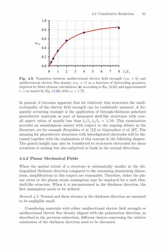
4.4 Constitutive Reduction 61
Fig. 4.9. Transition between unidirectional electric field strength (υ31 = 0) andunidirectional electric flux density (υ31 = 1) as a function of electroding geometrydepicted by finite element calculations (•) according to Eq. (4.25) and approximated(−) as stated by Eq. (4.26) with cf = 1.75.
In general, it becomes apparent that for relatively thin structures the unidi-rectionality of the electric field strength can be confidently assumed. A fre-quently occurring example is the application of through-thickness polarizedpiezoelectric materials as part of laminated shell-like structures with over-all aspect ratios of usually less than l3/l1, l3/l2 = 1/10. This examinationprovides an unambiguous answer with respect to the ongoing debate in theliterature, see for example Benjeddou et al. [12] or Gopinathan et al. [87]. Themeaning for piezoelectric structures with interdigitated electrodes will be dis-cussed together with the explanation of this concept in the following chapter.The gained insight may also be transferred to structures electroded for shearactuation or sensing but also subjected to loads in the normal directions.
4.4.2 Planar Mechanical Fields
When the spatial extent of a structure is substantially smaller in the dis-tinguished thickness direction compared to the remaining dominating dimen-sions, simplifications in this respect are reasonable. Therefore, either the pla-nar stress or the planar strain assumption may be employed for a such thin,shell-like structure. When it is unconstrained in the thickness direction, thefirst assumption needs to be utilized:
Remark 4.5. Normal and shear stresses in the thickness direction are assumedto be negligible small.
Considering materials with either unidirectional electric field strength orunidirectional electric flux density aligned with the polarization direction, asdescribed in the previous subsection, different choices concerning the relativeorientation of the thickness direction need to be discussed.

62 4 Piezoelectric Materials
Planar Stress Transverse to Polarization
Assuming planar stress as of Remark 4.5 on the plane perpendicular to thepolarization direction, see Figure 4.10(a), and thus aligning the latter withthe thickness direction, has the following implications and consequences whensubstituted into Eqs. (4.19) and (4.24):
σ3 = 0 → ε3 = −CE13
CE33
ε1 − CE23
CE33
ε2 +e33CE
33
E3 and
τ23 = 0 → γ23 = 0,τ31 = 0 → γ31 = 0.
(4.27)
Thereby the neglected shear stresses and consequently vanishing shear strains,given on the right-hand side of Eqs. (4.27), ensure complete constitutive equal-ity of both variants of Remark 4.4 for this configuration. This is, on the onehand, due to the discard of those coefficients in Eq. (4.24) representing thedifferences and, on the other hand, due to the ultimately vanishing transverseelectric flux densities to be found in the middle of Eqs. (4.22). With elimina-tion of the normal strain in thickness direction, the constitutive relation thentakes the following form:
⎧⎪⎪⎨
⎪⎪⎩
σ1
σ2
τ12D3
⎫⎪⎪⎬
⎪⎪⎭
=
⎡
⎢⎢⎢⎢⎢⎢⎣
CE11 − (CE
13)2
CE33
CE12 − CE
13CE23
CE33
0 −e31 + CE13
CE33e33
CE12 − CE
13CE23
CE33
CE22 − (CE
23)2
CE33
0 −e32 + CE23
CE33e33
0 0 CE66 0
e31 − CE13
CE33e33 e32 − CE
23CE
33e33 0 εε33 + (e33)
2
CE33
⎤
⎥⎥⎥⎥⎥⎥⎦
⎧⎪⎪⎨
⎪⎪⎩
ε1ε2γ12E3
⎫⎪⎪⎬
⎪⎪⎭
.
(4.28)
Planar Stress in Plane with Polarization
Assuming planar stress as of Remark 4.5 in the plane of the polarization di-rection, see Figure 4.10(b), and thus having the latter perpendicular to thethickness direction selected to be the e2-direction, has the following implica-tions and consequences when substituted into Eqs. (4.19) and (4.24):
σ2 = 0 → ε2 = −CE12
CE22
ε1 − CE23
CE22
ε3 +e32CE
22
E33 and
τ23 = 0 → γ23 = 0,τ12 = 0 → γ12 = 0.
(4.29)
Since no assumptions are made here concerning the piezoelectrically coupledshear behavior in the plane spanning between the e3- and e1-direction, the

4.4 Constitutive Reduction 63
Fig. 4.10. Correlation of polarization direction (P) and plane of planar stress.
two variants of Remark 4.4 for this configuration are still to be distinguishedby the additional term of the respective shear stiffness:
⎧⎨
⎩
σ3
σ1
τ31
D3
⎫⎬
⎭=
⎡
⎢⎢⎢⎢⎢⎢⎢⎣
CE33 − (CE
23)2
CE22
CE13 − CE
12CE23
CE22
0 −e33 +CE
23CE
22e32
CE13 − CE
12CE23
CE22
CE11 − (CE
12)2
CE22
0 −e31 +CE
12CE
22e32
0 0 CE55 + υ31
(e15)2
εε11
0
e33 − CE23
CE22
e32 e31 − CE12
CE22
e32 0 εε33 + (e32)2
CE22
⎤
⎥⎥⎥⎥⎥⎥⎥⎦
︸ ︷︷ ︸Q
⎧⎨
⎩
ε3
ε1
γ31
E3
⎫⎬
⎭.
(4.30)
4.4.3 Planar Rotation
By virtue of the assumptions of unidirectional electrostatic fields and planarmechanical stress, the electromechanically coupled constitutive relations havebeen modified significantly. In example, the formulation on the left-hand sideof Eq. (4.10a) reduces to Eq. (4.28) or (4.30). A transformation of coordi-nates on the considered plane may be performed as a rotation around theaxis normal to this plane. In the case of Eq. (4.30), the base vector e2 repre-sents the axis of rotation and thus this planar rotation may be formulated asfollows: ⎧
⎪⎪⎨
⎪⎪⎩
σx
σs
τxs
D3
⎫⎪⎪⎬
⎪⎪⎭
= TQTT
︸ ︷︷ ︸Q
⎧⎪⎪⎨
⎪⎪⎩
εxεsγxs
E3
⎫⎪⎪⎬
⎪⎪⎭
. (4.31)

64 4 Piezoelectric Materials
The transformation matrix T can be adapted from the spatial case of Eq. (4.14)by removing the unnecessary rows and columns. To account for the modifiedarrangement of components in Eq. (4.30), the respective rows and columnsalso need to be exchanged in the transformation matrix; it takes the followingform:
T =
⎡
⎢⎢⎣
cos2 α sin2 α 2 cosα sinα 0sin2 α cos2 α −2 sinα cosα 0
− sinα cosα cosα sinα cos2 α − sin2 α 00 0 0 1
⎤
⎥⎥⎦ . (4.32)
4.4.4 Negated Electric Field Strength
In the derived expression for the virtual work of internal contributions,Eq. (3.63), as well as in the definition of the electroelastic energy density,Eq. (3.64), the electric fields strength appears in a negated form representedby the vector E. With the adoption of such an arrangement in the asso-ciate constitutive relation, to be found on the left-hand side of Eq. (4.10a),it is possible to compensate for the unsymmetry in the matrix of constitutiveproperties C of the electromechanically coupled material. Thus a symmetricvariant C = C
T of this matrix may be introduced as follows:
{σD
}
︸ ︷︷ ︸Y
=[CE −eeT εε
]
︸ ︷︷ ︸C
{εE
}
︸ ︷︷ ︸Z
=[CE −eeT εε
] [I
−I
]{ε
− E
}
=[CE eeT −εε
]
︸ ︷︷ ︸C
{εE
}
︸ ︷︷ ︸Z
.
(4.33)
Correspondingly, the consequent modifications of the constitutive relationmay be treated. For the case of planar stress and unidirectional electric intransformed coordinates, this yields:
⎧⎪⎪⎨
⎪⎪⎩
σx
σs
τxs
D3
⎫⎪⎪⎬
⎪⎪⎭
= Q
⎡
⎢⎢⎣
1 0 0 00 1 0 00 0 1 00 0 0 −1
⎤
⎥⎥⎦
︸ ︷︷ ︸Q
⎧⎪⎪⎨
⎪⎪⎩
εxεsγxs
E3
⎫⎪⎪⎬
⎪⎪⎭
. (4.34)
Electroelastic Energy Density
In Section 3.5.1, Dirichlet’s principle of minimum potential energy has beenextended to electromechanically coupled problems. With the exception of re-ferring to the required potential property, the electroelastic energy density U0
has not yet been further specified. With Eq. (3.64) a second relation linkingthe fields of the constitutive relation is available, such that it may be used

4.5 Actuator and Sensor Conditions 65
to determine the electroelastic energy density U0. This leads to the followingformulation:
U0 =12
{
εT ET}[CE e
eT −εε
]
︸ ︷︷ ︸C
{εE
}
with E = −E, C = CT . (4.35)
It can be verified by substitution into Eq. (3.64) which should result in theconstitutive relation. Thus it becomes apparent that the utilized matrix ofconstitutive properties has to be symmetric. While this is given for the for-mulation with the matrix C introduced on the right-hand side of Eq. (4.33),the conventional variant C to the left-hand side proves to be of no avail.
4.5 Actuator and Sensor Conditions
In Section 4.3, the piezoelectric effect has been examined in an illustrativemanner with respect to actuation and sensing. To quantify these findingsfor more complicated structures, calculation procedures can be developed,based on the principle of virtual work derived in Section 3.4. Therefore, thedifferent variants of actuation, depending on the type of electric power supply,and of sensing, depending on the type of measurement, will be studied herewith regard to the associated boundary conditions. Without practical loss ofgenerality, the following simplification may be introduced for all instances:
Remark 4.6. For the actual application of piezoelectric materials, free chargesin the volume are excluded.
qΛ = 0. (4.36)
Since no volume charges qΛ will be specified, the corresponding term inthe virtual work of external charges δV ep vanishes, see Eqs. (3.53) and (3.62)respectively.
4.5.1 Actuator Application with Voltage and Current Source
To induce mechanical deformation with an actuator based on piezoelectricmaterial, electric power needs to be supplied. In electrical engineering, twoideal power sources are distinguished. A voltage source provides a constantvoltage, while the wattage may then be adjusted via the current. A currentsource the other way round keeps the current constant, while the wattage maythen be adjusted via the voltage.
Voltage Source
When a voltage source is connected to the electrodes of a piezoelectric actu-ator, the electric potential ϕ is prescribed. This includes the compensation

66 4 Piezoelectric Materials
of possibly superimposed mechanical influences. So the electric potential ϕdoes not represent an unknown, and thus its variation δϕ vanishes as well asthe variation of the electric field strength δE in consideration of Eq. (3.39).Therewith, all contributions of the principle of virtual electric potential ofEq. (3.53) disappear:
δϕ = 0 → δV ep = 0, δE = 0 → δU ep = 0. (4.37)
Hence, the principle of virtual work of Eqs. (3.62) and (3.63) reduces to itsmechanical part. Via the dependence of mechanical stresses σ = σ(ε,E) in theelectromechanically coupled constitutive relation, see Eq. (4.17), the electricfield strength E however enters the formulation as a parameter:
∫
Λ
δεT σ + δuT aρdV =∫
∂Λσ
δuT f∂Λ dA+∫
Λ
δuT fΛ dV . (4.38)
Current Source
When a current source is connected to the electrodes of a piezoelectric actu-ator, the electric potential ϕ is unknown. Therefore, the contributions of theprinciple of virtual electric potential of Eq. (3.53) need to be retained. Sincethe current describes the derivative trend of charge with respect to time, itprescribes the area charge q∂Λ on the electrodes. An adequate formulation ofthe principle of virtual work from Eqs. (3.62) and (3.63), in consideration ofEq. (4.36), reads
∫
Λ
{
δεT δET}{
σD
}
+ δuT aρdV
=∫
∂Λ
{δuT −δϕ
}{
f∂Λ
q∂Λ
}
dA+∫
Λ
δuT fΛ dV . (4.39)
4.5.2 Sensor Application with Voltage and Current Measurement
The different variants of the sensor application have become obvious fromobserving Figure 4.5. A mechanical load on piezoelectric material induces anelectric field strength field when the electrodes are disconnected and an electricflux density field when the electrodes are connected. This corresponds to thepossibilities of measurement of electric quantities. As with the actuator appli-cation, only the ideal cases shall be considered here, leaving the complicationsof the actual circuits, including the necessary amplification, to the competentelectrical engineering literature, see for example Tichy and Gautschi [174].
Strain Sensor–Voltage Measurement
To determine the voltage, a measuring instrument with high inherent resis-tance is used such that the current and thus the flow of charges is low. In the

4.5 Actuator and Sensor Conditions 67
ideal case, this corresponds to disconnected electrodes. Then the difference ofelectric potential ϕ at the opposing electrodes and, consequently, the electricfield strength E can be determined without changing the area charge q∂Λ onthe electrodes. In practical applications, the latter is often zero, see Carpen-ter [43]. To simulate the outcome of such a measurement proportional to thestrain state, it may be proceeded from Eq. (4.39) as well.
Strain Rate Sensor–Current Measurement
To determine the current, a measuring instrument with low inherent resis-tance is used such that the caused voltage drop is low. In the ideal case, thiscorresponds to connected electrodes. Then the difference of electric potentialϕ at the opposing electrodes levels out, and thus the electric field strength Eis cancelled. This permits us to draw the conclusions as of Eq. (4.37). Conse-quently, the mechanical state of the system can be determined with the aidof the principle of virtual work formulation of Eq. (4.38). Via the electro-mechanically coupled constitutive relation, the outcome may then be utilizedto deduce the electric flux density, charge, and finally the current being pro-portional to the strain rate.
5
Piezoelectric Composites
The integration of piezoelectric materials into composites allows for the im-provement of constitutive properties as well as of failure behavior and con-sequently for an extension of the application spectrum. So this chapter isconcerned with the conception and modeling of such piezoelectric compositesfor structural applications. For the prediction of the effective composite prop-erties, different methodologies of micro-electromechanics are investigated andvalidated through experiments and finite element analyses.
5.1 Classification of General Composites
Composites provide the possibility to combine the advantageous characteris-tics of different materials and qualities are often achieved that none of the con-stituents possesses. Essential criteria in general are stiffness, strength, weight,damping, thermal and electric conductivity, as well as resistance against envi-ronmental influences, wear, and fatigue. Further on they make possible the op-timization of anisotropic mechanical, thermomechanical, and electromechani-cal couplings. Introductory literature on composites is provided, for example,by Jones [107], Altenbach et al. [6], Chawla [50], Matthews and Rawlings [123].Besides a classification by means of the constituent materials, composites maybe distinguished by the spatial arrangement of the material phases. To be acomposite at least two such phases need to occur whereby the matrix phasesurrounds and connects one or more inclusion phases.
5.1.1 Topology of the Inclusion Phase
The diverse shapes of inclusions may be used for a classification of composites,as shown for the basic cases of particulate, fibrous, and lamellar topologiesin Figure 5.1. There are also composites which represent a combination ofthese inclusion types. In steel concrete, for example, mineral particles andmetal fibers are joined by a binder material. For aerospace applications, the
T.H. Brockmann, Theory of Adaptive Fiber Composites,Solid Mechanics and Its Applications 161,c© Springer Science + Business Media B.V. 2009

70 5 Piezoelectric Composites
combination of glass fibers and aluminum laminae is becoming increasinglypopular. The listed types of inclusions may be further categorized with respectto their geometry and relative arrangement. In the case of fibrous inclusions,there are continuous or discontinuous fibers of straight or curled shape ina regular or irregular layout. More complicated fiber structures arise whentextile techniques like stitching, braiding, or knitting are involved, see forinstance Poe et al. [142] or Cox and Flanagan [57].
Fig. 5.1. Classification of composites by the spatial extent of inclusions: (a) partic-ulate, (b) fibrous, (c) lamellar.
5.1.2 Laminated Composites and Laminated Fiber Composites
A prominent position is taken by the combination of lamellar inclusions ofcontinuous as well as planar extent with only a small amount of matrix ma-terial. This description in terms of the above classification is synonymouswith monolithic laminae bonded with a thin film of adhesive representingthe widely used concept of laminated composites. The individual laminae donot necessarily have to be monolithic but may consist of composite materi-als again. With the contained inclusions being existent in fibrous shape, theoutcome is a laminated fiber composite. Especially, the case of continuous,straight, and parallel fibers is of great importance with regard to lightweightstructures. Corresponding to their setup, the analysis of laminated fiber com-posites may be organized in two steps to be subsequently demonstrated inconsideration of electromechanically coupled materials. First, on the level ofmicro-electromechanics in this chapter, the effective properties of the laminaeare determined from the characteristics of matrix and inclusions. Second, onthe level of macro-electromechanics in the next chapter, the effective proper-ties of the laminate are determined from the characteristics of the laminae.
5.2 Conception of Piezoelectric Composites
To enable actuation and sensing of structures with laminar elements like platesand shells, the application of piezoelectric materials is well established. In the

5.2 Conception of Piezoelectric Composites 71
simplest case, monolithic ceramic materials are attached in the form of thinpatches on one or both sides. In view of the above discussion, such an assemblyconstitutes a laminated composite. For any case of structural deformation,the aspired effective direction of the piezoelectric effect lies in the plane of thepiezoelectric laminae. Initially areal electrodes on its top and bottom surfacehave been employed to provide or perceive the electrostatic field respectively,Figure 5.2(a). To avoid unintentional and possibly creeping repolarization, thedirections of polarization and electric field strength should be aligned. Thus,both of these directions are oriented normal to the plane of the consideredpatch and only the minor piezoelectric effect in the isotropic transverse plane,as e31 < e33 and d31 < d33 to be found in Table A.3, can be exploited.
Fig. 5.2. Variants of patches for actuation or sensing: (a) monolitic material withareal electrodes, (b) monolitic material with interdigitated electrodes, (c) fiber com-posite with areal electrodes, (d) fiber composite with interdigitated electrodes.
5.2.1 Interdigitated Electrodes and Piezoelectric Fibers
To increase the electromechanical coupling and allow for anisotropic and thusdirectional actuation and sensing, the concept of interdigitated electrodes hasbeen introduced by Hagood et al. [90] for monolithic piezoelectric laminae,as shown in Figure 5.2(b). Thereby in-plane placement of the parallel direc-tions of polarization and electric field strength is permitted. These directions

72 5 Piezoelectric Composites
jointly change sign from one interval between opposing polarity electrodes tothe next and, in this manner, assure uniform behavior, see Figure 5.3. Tocompensate for the drawbacks caused by the brittle and inflexible nature ofceramic materials, the embedding of piezoelectric materials in the form offibers into a polymer matrix has been implemented by Bent et al. [16,17] forareal electrodes, as shown in Figure 5.2(c). Thus, besides increased strengthand conformability the advantageous possibility of optimizing the anisotropicproperties is also gained. Further improvements are achieved when, in addi-tion, interdigitated electrodes are applied, Bent and Hagood [14,15], as shownin Figure 5.2(d).
Fig. 5.3. Sectional view of the interdigitated electroding scheme with qualitativedistribution of lines of electric field strength (E) and directions of polarization (P).
5.2.2 Electroding Implications
As examined in detail in Section 4.4, it is possible to simplify the constitutiverelation of piezoelectric materials in consideration of loading, electroding, andassociated geometry of the structure. The two variants of electroding intro-duced above have different implications.
Areal Electrodes
In the case of areal electrodes, as shown in Figures 5.2(a) and (c), the out-of-plane shear modes suggest, for the small characteristic ratio of thicknessto the other extents of the laminae, the assumption of unidirectional elec-tric field strength in polarization/through-thickness direction, compare withFigure 4.8(b). When only planar stress in the plane transverse to the polar-ization direction is regarded, then the constitutive relation anyway reduces toEq. (4.28).
Interdigitated Electrodes
While for areal electrodes, the in-plane shear mode is free of electromechanicalcoupling, a structure with interdigitated electrodes, as shown in Figures 5.2(b)

5.2 Conception of Piezoelectric Composites 73
and (d), exhibits such a coupling. The characteristic ratio relates the spac-ing between electrodes to the length of the electrode fingers. This again isvery small for the existent specimens, see for example Figure 5.4. The othermode of electromechanically coupled shear occurs in the plane unfolding be-tween the through-thickness (e2) and the polarization (e3) direction. Here theelectric connection of the electrode pairs on the top and bottom sides, seeFigure 5.3, leads to a non-homogeneous behavior in analogy to both casesof Figure 4.6(b). The conditions underneath the electrodes correspond to thecase with connected electrodes, while the situation in the intervals betweenopposing polarity electrodes resembles the case without electrodes. When onlyplanar stress in the plane of the laminae is regarded, this out-of-plane shearmode is discarded and the in-plane shear mode, as discussed above, impliesυ31 = 0 in the associated constitutive relation of Eq. (4.30).
Fig. 5.4. NASA Langeley Research Center (LaRC) Macro-Fiber Composite (MFC);original photograph by the National Aeronautics and Space Administration [130].
5.2.3 Development Status
A number of different approaches to realizing composites with piezoelectricfibers and interdigitated electrodes have been developed or proposed. Thesemay be distinguished by the process of fiber production and the applicationof electrodes. Suitable fibers can be fabricated in a sintering process frompiezoelectric powders with techniques like extrusion of polymer supportedpowders, Strock et al. [171], or sol-gel spinning, Helbig et al. [92]. With theco-extrusion of a tube of polymer-supported piezoelectric powder filled andsurrounded by material to be burned off afterwards, it is possible to pro-duce hollow fibers, Cannon and Brei [42]. For these complex manufacturingprocesses, a greater number of parameters needs to be established and con-trolled in order to maintain the required quality. Less complicated and costlyis the dicing of monolithic piezoelectric materials into rectangular fibers pro-viding good accuracy and repeatability, Wilkie et al. [182]. Several differenttypes of electrodes have been discussed. Interlaminar electroding structures

74 5 Piezoelectric Composites
attached to the top and bottom sides of a piezoelectric laminae, as depictedin Figures 5.2(b) and (d), have been realized by etching copper on a support-ing film, see for example Bent and Hagood [14] or Wilkie et al. [182]. Suchfilms package the laminae and thus provide insulation to other possibly con-ductive laminae, for example when carbon fibers are contained. To take theelectrodes closer to the fibers, the use of conductive adhesives was investigatedby Pannkoke et al. [136]; rings of silver paint have been applied on the insideand outside of hollow fibers by Cannon and Brei [42]; and linked conductiverings around solid circular fibers have been proposed by Tan and Tong [173].So far, only the combination of diced rectangular fibers made of PZT-5H-typematerial with interlaminar copper electrodes has reached batch production,High and Wilkie [94], see Figure 5.4. A research application of such actuatorsto alleviate the buffet effect at twin tail aircraft, Sheta et al. [162], is shownin Figure 5.5. A promising development direction of this actuator concept isthe employment of fibers made of single crystal PMN-PT-type materials, asreported by Wilkie et al. [183], with significantly improved electromechanicalcoupling properties, compare Section 4.1.2 and Table A.3. Further surveyswith respect to piezoelectric fiber composites are given by Williams and In-man [184] as well as by Nelson [132]. A comparison of the performance ofpackaged piezoelectric actuators for industrial applications representing allfour variants of Figure 5.2 has been conducted by Pretorius et al. [145].
Fig. 5.5. Scaled model of a vertical tail fin with applied macro-fiber compositeactuator patches; original photograph by the National Aeronautics and Space Ad-ministration [130].
5.2.4 Representative Volume Element and Fiber Geometry
While a composite as the whole thing is a rather complicated structure, theessential relations may be illustrated by means of a small but representative

5.2 Conception of Piezoelectric Composites 75
piece of it. Such a representative volume element therefore is utilized as thebasis of some analysis approaches. In order to portray the characteristics ofthe entire composite, it will be defined as follows:
Remark 5.1. A representative volume element is the smallest region of thecomposite over which mechanical as well as electrostatic fields are macroscop-ically uniform.
On account of the heterogeneous properties of the constituents, these fieldsare likely to be microscopically non-uniform. Accordingly, the appropriategeometry and boundary conditions need to be identified. Size and complexityof a representative volume element depend on the topology of the compos-ite. Elaborate configurations are necessary, for example, to embody textilecomposites, whereas the consideration of a single inclusion together with theconnected portion of matrix material is often sufficient. Furthermore, advan-tage can be taken of the symmetry of the examined region, being especiallyvaluable for the finite element discretization. Such a simplified representativevolume element is shown in Figure 5.6 for a composite patch with a singlefiber layer. It contains a quarter of the cross-section of fiber and surround-ing matrix and its length may be limited to half of the electrode spacing. Inthe conventional case without electromechanical coupling, the length in direc-tion of the fiber is arbitrary, since stresses and strains do not vary along thisdirection.
Fig. 5.6. Simplified representative volume element in consideration of fibrous in-clusions and interdigitated electrodes.
Fiber Volume Fraction
The essential statement about the composition of the considered composite isprovided by the fiber volume fraction ν. As the material distribution does not

76 5 Piezoelectric Composites
change along the fiber direction, only the geometric relations in the plane ofthe fiber cross-section are relevant. The associated directional fiber fractionsν1 and ν2 may be determined from the fiber dimensions af
1 and af2 and fiber
spacings a1 and a2:
ν1 =af1
a1, ν2 =
af2
a2, (5.1a)
ν = ν1ν2. (5.1b)
The characteristic cross-sectional dimensions are depicted together with elec-trode spacing a3 and electrode width b3 in Figure 5.7 by means of the simpli-fied representative volume element.
Fig. 5.7. Characteristic dimensions of the simplified representative volume element.
Fiber Cross-Sectional Shape
The cross-sectional shape of the fibers is primarily of local importance, forinstance with respect to stress concentrations along the edges. Aiming at thedetermination of the overall behavior, only the directional fiber fractions haveto be considered. This is equivalent to the mapping of an arbitrary shape ontoa rectangle with the appropriate edge lengths for approaches based on repre-sentative volume elements like the one outlined above. For other approacheswith an elliptic elementary fiber shape, it can be proceeded correspondinglyby determining the appropriate ellipticity coefficient. Further insight may begained using the method of cells presented by Aboudi [1,2]. It divides the rep-resentative volume element into subcells with interfacial conditions and thusallows for a discretization of the fiber cross-section. The examination of slicesof the simplified representative volume element is considered in the work ofTan and Tong [173].
5.3 Micro-Electromechanics with Equivalent Inclusions 77
5.2.5 Modeling Preliminaries
To continue the analysis of laminae with piezoelectric fibers just as in themonolithic case, it is necessary to homogenize the heterogeneous propertiesof fibers and matrix. Thus, the objective is to determine the presupposedlyhomogeneous overall behavior of the composite based on the known character-istics of the individual constituents and their interaction. For this purpose, inthe context of conventional composites, a greater number of theories has beendeveloped and several have been extended to capture the implications of thepiezoelectric effect. In general, the analytical homogenization methods may beroughly subdivided into two categories. On the one hand there are approacheswhich make use of the “Theory of Elasticity” as completely as possible, whileon the other hand approaches utilize ad hoc assumptions within the frame-work of the “Mechanics of Materials”. Representatives of both categories willbe investigated in the subsequent sections. Although these approaches possessdiverging abilities, which will be indicated individually, the current require-ments will function as a common foundation.
Remark 5.2. The subsequent discussion of micro-electromechanical approachesto determine the macroscopic constitutive properties of a composite will beconcentrated on properties within the following categories:
• Constituents→ homogeneous, linearly elastic materials with piezoelectric properties.
• Topology→ continuous, straight, perfectly aligned and regularly spaced fibers.
• Connection→ perfect bonding of constituents, no direct contact between inclusions.
Typically, the fiber material is at most transversely isotropic, Eq. (4.17)with Eqs. (4.3), (4.8), and (4.18), while the matrix material is isotropic,Eq. (4.17) with Eqs. (4.4), (4.9), and vanishing piezoelectric moduli. Thesubsequent theories are not confined to such a behavior. However, it will bepresumed that the distinguished axes are aligned. Deviating cases may be con-sidered in conjunction with an appropriate transformation, see Section 3.2.5.In accordance with the considerations of Section 4.4.4, the notation with anegated electric field strength will be utilized throughout the entire chapter.
5.3 Micro-Electromechanics with Equivalent Inclusions
The micro-electromechanical methodology stemming from the category of the“Theory of Elasticity” to be presented in this section is capable of modelinginclusions of ellipsoidal geometry. Such a description of the inclusion geometryallows us to consider fibrous and lamellar inclusions by means of one or twosemiaxes approaching infinity, respectively.

78 5 Piezoelectric Composites
5.3.1 Mean Fields and Concentration Matrices
Subjecting a homogeneous body to homogeneous boundary conditions resultsin homogeneous fields. These homogeneous fields can be shown to agree withthe volumetric average of the fields found in a non-homogeneous body exposedto identical boundary conditions, see Aboudi [1] or Dunn and Taya [66]. Con-sequently, these mean macroscopic fields may be expressed as an average ofthe mean fields inherent to the individual material phases weighted by theirvolume fraction. For electromechanically coupled composites with the volumefraction ν of a single inclusion phase, this leads to
Z = νZi + (1 − ν) Zm, (5.2a)
Y = νY i + (1 − ν) Y m. (5.2b)
Mean stresses and electric flux densities Y as well as mean strains and elec-tric field strengths Z are composed of the corresponding mean fields in theinclusion and matrix phase as indicated by the superscripts i and m. Cross-connecting these fields, the constitutive relations of the homogenized compos-ite, as well as of the individual material phases, may be given as follows:
Y = CZ, Y i = CiZ
i, Y m = CmZ
m. (5.3)
The unique dependence of strains and electric field strengths as well as stressesand electric flux densities in the individual material phases upon the overallfields of the composite may be formulated with the aid of the concentrationmatrices Ξi and Ξm, respectively, Σi and Σm:
Zi = ΞiZ, Z
m = ΞmZ, with νΞi + (1 − ν)Ξm = I; (5.4)
Y i = ΣiY , Y m = ΣmY , with νΣi + (1 − ν)Σm = I. (5.5)
Starting off with Eq. (5.2b) and subsequent substitution of stresses and electricflux densities Y , Y i, and Y m from the constitutive relations of Eq. (5.3), ofstrains and electric field strengths Z
m from Eq. (5.2a) and Zi from Eq. (5.4),
the effective properties may be written as
C = ν(C
i − Cm)Ξi + C
m. (5.6)
Analogously, the inverted representation, see Eqs. (4.10), may be treated inconsideration of Eq. (5.5), leading to
(C)−1 = ν
((C
i)−1 −
(C
m)−1
)Σi +
(C
m)−1 . (5.7)
Thus, the effective properties C of a composite are described in Eqs. (5.6) and(5.7) by the known fiber volume fraction ν and constituent properties C
i andC
m, as well as by the concentration matrices Ξi and Σi of the inclusion phaseto be determined by the succeeding theories.

5.3 Micro-Electromechanics with Equivalent Inclusions 79
5.3.2 Elementary Rules of Mixture
For the sake of comprehensiveness and later comparison, the most elementaryoptions to determine the overall properties of a composite will be given herefor the derived formulation. Assumptions in analogy to parallel and seriesconnections of springs typical for the “Mechanics of Materials” are utilized,dating back to the works of Voigt [175] and Reuss [154]. The assumptionof uniform strains and electric field strengths Z
i = Zm = Z leads with
Eqs. (5.4) to the concentration matrices Ξi = Ξm = I. Applied to Eq. (5.6),such a parallel connection of material phases results in the weighted additionof the electroelastic moduli:
C = νCi + (1 − ν) Cm. (5.8)
Correspondingly, the assumption of uniform stresses and electric flux den-sities Y i = Y m = Y leads with Eqs. (5.5) to the concentration matricesΣi = Σm = I. Applied to Eq. (5.7), such a series connection of materialphases results in the weighted addition involving the inverse matrices of theelectroelastic moduli:
(C)−1 = ν
(C
i)−1
+ (1 − ν)(C
m)−1
→ C =(ν(C
i)−1
+ (1 − ν)(C
m)−1
)−1
. (5.9)
The above assumptions, however, have incorrect implications. For a parallelconnection of material phases, the equilibrium conditions are violated at phaseboundaries, while for a series connection of material phases, the compatibilityconditions may not hold at phase boundaries. Nevertheless, it can be shownthat these estimates may serve as upper and lower bounds enclosing the actualelectroelastic moduli of the composite. For a discussion of bounds on effectiveelastic properties, see Christensen [54].
5.3.3 Equivalence of Inclusion and Inhomogenity
Let there be a homogeneous ellipsoidal inclusion filling the domain Λi withthe electroelastic properties C
i embedded into an infinite homogeneous matrixwith the electroelastic properties C
m. Such a composite filling the domain Λwill be subjected to uniform boundary conditions
Y ∂Λ = Y , respectively Z∂Λ = Z. (5.10)
The overall strains and electric field strengths Z of the composite can beeither interpreted as a response to the applied stresses and electric flux den-sities or are the direct implication of the boundary conditions. In absenceof the inclusion, they would prevail throughout the domain Λ. The resultingstrains and electric field strengths Z
i inside the inclusion may be assembled

80 5 Piezoelectric Composites
in consideration of perturbation fields Z• caused by the deviating material
properties of the inclusion:Z
i = Z + Z•. (5.11)
Thus, the stresses and electric flux densities inside the inclusion can be deter-mined from the corresponding constitutive relation of Eq. (5.3) as
Y i = Ci(Z + Z
•)
. (5.12)
The considered inclusion may be replaced by matrix material subjected toadditional so-called eigenfields Z
∗ such that the stresses and electric fluxdensities inside the domain Λi remain unchanged and thus can be describedby
Y i = Cm(Z + Z
• − Z∗)
. (5.13)
The equivalence of an inclusion with deviating material properties and aninhomogenity on account of eigenfields has been introduced for the elasticcase by Eshelby [73] and extended to the piezoelectric case by Deeg [61]. Itwas shown that the eigenfields Z
∗ are uniform for an ellipsoidal shape of thedomain Λi. In conjunction with the presumed uniform boundary conditions onthe enclosing surface ∂Λ at infinite distance, this leads to an entirely uniformdistribution of fields inside the domain Λi. Therefore, a linear transformationbetween perturbation fields Z
• and eigenfields Z∗ can be established:
Z• = ΥZ
∗. (5.14)
The constraint matrix Υ depicts the effect of the constraining matrix on theinclusion and is a function of matrix material properties and ellipsoidal inclu-sion shape. It represents the piezoelectric analog to Eshelby’s tensor in theelastic case, see Dunn and Taya [66]. Expressions for cylindrical inclusionsto model fibrous composites are provided by Dunn and Taya [67] (this refer-ence uses a different notation, Υ is called S). Equating Eqs. (5.12) and (5.13)and making use of Eq. (5.14) to replace the eigenfields Z
∗ and Eq. (5.11) toeliminate the perturbation fields Z
• after some manipulations, leads to
Zi =
(I + Υ
(C
m)−1 (
Ci − C
m))−1
︸ ︷︷ ︸Ξi
dil
Z. (5.15)
The concentration matrix Ξidil may be identified with the aid of Eq. (5.4).
As its derivation is based on a single inclusion within an infinite matrix,it is applicable only to very low volume fractions of the inclusion or fiberphases, respectively. Such a configuration is usually denominated as a diluteconcentration.

5.3 Micro-Electromechanics with Equivalent Inclusions 81
5.3.4 Non-Dilute Concentrations
To accomplish their specific task, most of composites require a portion ofthe inclusion phase that certainly cannot be described as dilute. Therefore,methods based on the equivalence of inclusion and inhomogenity derived abovehad to be developed to extend the range of applications to practicable volumefractions.
Mori–Tanaka Approach
Almost a standard procedure, due to its relative simplicity while allowing fordependable results and documented by a thorough theoretical discussion inthe literature, the Mori–Tanaka approach was initiated by Mori and Tanaka[127]. Its major assumption may be formulated for electromechanically cou-pled composites as follows:
Remark 5.3. Strains and electric field strengths inside an inclusion in the non-dilute case behave with respect to the average fields of the matrix phase justlike they would do in the dilute case with respect to the overall fields of thecomposite.
Zi = Ξi
dilZm. (5.16)
Since the overall fields of the composite with dilute concentration alreadyaccount for the interaction between inclusion and matrix, this means that theinclusion is now considered to be embedded into a matrix containing otherinclusions. Eliminating strains and electric field strengths Z
m of the matrixphase in Eq. (5.2a) by utilization of Eq. (5.16) results after a few manipulationsin
Zi = Ξi
dil
(νΞi
dil + (1 − ν) I)−1
︸ ︷︷ ︸Ξi
MT
Z. (5.17)
Again, the concentration matrix ΞiMT for the Mori–Tanaka approach can be
identified with the aid of Eq. (5.4). It has been proposed in this form for theelastic case by Benveniste [18] and extended to the piezoelectric case by Dunnand Taya [67].
Other Approaches
There are a number of other ways to consider non-dilute concentrations withinequivalent inclusion approaches. Among them are the self-consistent schemes,see Aboudi [1], where an inclusion is examined that is surrounded in theclassical variant by an effective medium of a priori unknown properties andthe generalized variant by matrix material, which again is embedded into suchan effective medium. The resulting concentration matrices are comparable tothe dilute case of Eq. (5.15), but with fundamental difference of a dependence
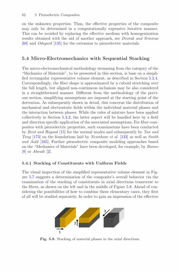
82 5 Piezoelectric Composites
on the unknown properties. Thus, the effective properties of the compositemay only be determined in a computationally expensive iterative manner.This can be avoided by replacing the effective medium with homogenizationresults obtained with the aid of another approach, see Dvorak and Srinivas[68] and Odegard [135] for the extension to piezoelectric materials.
5.4 Micro-Electromechanics with Sequential Stacking
The micro-electromechanical methodology stemming from the category of the“Mechanics of Materials”, to be presented in this section, is base on a simpli-fied rectangular representative volume element, as described in Section 5.2.4.Correspondingly, the fiber shape is approximated by a cuboid stretching overthe full length, but aligned non-continuous inclusions may be also consideredin a straightforward manner. Different from the methodology of the previ-ous section, simplifying assumptions are imposed at the starting point of thederivation. As subsequently shown in detail, this concerns the distribution ofmechanical and electrostatic fields within the individual material phases andthe interaction between phases. While the rules of mixture have been appliedcollectively in Section 5.3.2, the latter aspect will be handled here by a fieldand direction specific application of the associated assumptions. For fiber com-posites with piezoelectric properties, such examinations have been conductedby Bent and Hagood [15] for the normal modes and subsequently by Tan andTong [173] on the foundations laid by Newnham et al. [133] as well as Smithand Auld [165]. Further piezoelectric composite modeling approaches basedon the “Mechanics of Materials” have been developed, for example, by Banno[8] or Aboudi [2].
5.4.1 Stacking of Constituents with Uniform Fields
The visual inspection of the simplified representative volume element in Fig-ure 5.7 suggests a determination of the composite’s overall behavior via theexamination of the stacking of constituents in axial directions transverse tothe fibers, as shown on the left and in the middle of Figure 5.8. Ahead of con-sidering the possibilities of how to combine these elementary cases, they firstof all will be studied separately. In order to gain an impression of the effective
Fig. 5.8. Stacking of material phases in the axial directions.

5.4 Micro-Electromechanics with Sequential Stacking 83
properties of such a stack of two materials, its response to all load cases needsto be tested. Being subjected to arbitrary homogeneous boundary conditions,the mechanical and electrostatic fields within the individual material phasesmay not be entirely homogeneous in consequence of the dissimilar materialproperties. Since such effects are predominantly of local importance, they willbe neglected by virtue of the uniform fields assumption:
Remark 5.4. Mechanical and electrostatic fields are assumed to be homoge-neous throughout the individual material phases.
As the entire composite structure happens to be assembled from simplifiedrepresentative volume elements by symmetric completion and repetition, theedges have to remain straight and parallel in any event. Transferred to themechanical and electrostatic fields, this requirement may be fulfilled on thegrounds of the following assumption:
Remark 5.5. The macroscopic mechanical and electrostatic fields either coin-cide with field quantities found to be identical in all material phases or resultfrom the average of field quantities in the individual material phases weightedby their directional fraction in accordance with the scheme of Table 5.1.
Table 5.1. General assumptions for the stacking of material phases with respect tothe relation of macroscopic to microscopic mechanical and electrostatic fields.
Stress/El. Flux Density Strain/El. Field Strength
Stacking Direction coincidence weighted averageTransverse Plane weighted average coincidence
These assumptions can be applied immediately in the directions e1 and e2of the cross-sectional plane of the fibers. As the constitutive relation of theconsidered piezoelectric materials exhibits only a partial electromechanicalcoupling, normal modes and each of the shear modes may be treated inde-pendently, as illustrated by Eqs. (4.19) to (4.21). In accordance with the con-siderations of Section 4.4.4, the notation with negated electric field strengthand the associated constitutive submatrices E, G1, and G2 will be utilized.
5.4.2 Normal Mode Stacking Coefficients
The implications of Remark 5.5 are summarized in Table 5.2 for the stackingof material phases transverse to the fiber direction with respect to fields asso-ciated with the normal modes. While the macroscopic mechanical and electro-static fields carry the usual denominations, the association with the individualphases is indicated by the superscripts f and m for fields in the fiber and ma-trix phase respectively. The normal mode constitutive relation of Eq. (4.19)

84 5 Piezoelectric Composites
Table 5.2. Assumptions for the stacking of material phases with respect to normalmodes.
Direction Stress/El. Flux Density Strain/El. Field Strength
e1 σ1 = σf1 = σm
1 ε1 = ν1εf1 + (1 − ν1) εm
1
σ2 = ν1σf2 + (1 − ν1) σm
2 ε2 = εf2 = εm
2
σ3 = ν1σf3 + (1 − ν1) σm
3 ε3 = εf3 = εm
3
D3 = ν1Df3 + (1 − ν1) Dm
3 E3 = Ef3 = Em
3
e2 σ1 = ν2σf1 + (1 − ν2) σm
1 ε1 = εf1 = εm
1
σ2 = σf2 = σm
2 ε2 = ν2εf2 + (1 − ν2) εm
2
σ3 = ν2σf3 + (1 − ν2) σm
3 ε3 = εf3 = εm
3
D3 = ν2Df3 + (1 − ν2) Dm
3 E3 = Ef3 = Em
3
can be rewritten for every material phase in terms of those mechanical andelectrostatic fields that are identical in all material phases. For the stacking inthe e1- and e2-directions with the associated partially inverted matrices F
f1 ,
Fm1 and F
f2 , F
m2 of normal mode constitutive coefficients, this yields:
e1:
⎧⎪⎪⎪⎪⎨
⎪⎪⎪⎪⎩
εf1
σf2
σf3
Df3
⎫⎪⎪⎪⎪⎬
⎪⎪⎪⎪⎭
= Ff1
⎧⎪⎪⎨
⎪⎪⎩
σ1
ε2ε3E3
⎫⎪⎪⎬
⎪⎪⎭
,
⎧⎪⎪⎪⎨
⎪⎪⎪⎩
εm1σm
2
σm3
Dm3
⎫⎪⎪⎪⎬
⎪⎪⎪⎭
= Fm1
⎧⎪⎪⎨
⎪⎪⎩
σ1
ε2ε3E3
⎫⎪⎪⎬
⎪⎪⎭
, (5.18a)
e2:
⎧⎪⎪⎪⎪⎨
⎪⎪⎪⎪⎩
σf1
εf2
σf3
Df3
⎫⎪⎪⎪⎪⎬
⎪⎪⎪⎪⎭
= Ff2
⎧⎪⎪⎨
⎪⎪⎩
ε1σ2
ε3E3
⎫⎪⎪⎬
⎪⎪⎭
,
⎧⎪⎪⎪⎨
⎪⎪⎪⎩
σm1
εm2σm
3
Dm3
⎫⎪⎪⎪⎬
⎪⎪⎪⎭
= Fm2
⎧⎪⎪⎨
⎪⎪⎩
ε1σ2
ε3E3
⎫⎪⎪⎬
⎪⎪⎭
. (5.18b)
Furthermore, those mechanical and electrostatic fields that are assumed tobe a weighted average, as stated in Table 5.2, may be arranged collectively.Then the vectors of the phase specific fields can be replaced by substitutionof Eqs. (5.18a) and (5.18b), respectively:
e1:
⎧⎪⎪⎨
⎪⎪⎩
ε1σ2
σ3
D3
⎫⎪⎪⎬
⎪⎪⎭
= ν1
⎧⎪⎪⎪⎪⎨
⎪⎪⎪⎪⎩
εf1
σf2
σf3
Df3
⎫⎪⎪⎪⎪⎬
⎪⎪⎪⎪⎭
+ (1 − ν1)
⎧⎪⎪⎪⎨
⎪⎪⎪⎩
εm1σm
2
σm3
Dm3
⎫⎪⎪⎪⎬
⎪⎪⎪⎭
=(νf1 F
f1 + (1 − ν1) F
m1
)
︸ ︷︷ ︸F1
⎧⎪⎪⎨
⎪⎪⎩
σ1
ε2ε3E3
⎫⎪⎪⎬
⎪⎪⎭
,
(5.19a)
e2:
⎧⎪⎪⎨
⎪⎪⎩
σ1
ε2σ3
D3
⎫⎪⎪⎬
⎪⎪⎭
= ν2
⎧⎪⎪⎪⎪⎨
⎪⎪⎪⎪⎩
σf1
εf2
σf3
Df3
⎫⎪⎪⎪⎪⎬
⎪⎪⎪⎪⎭
+ (1 − ν2)
⎧⎪⎪⎪⎨
⎪⎪⎪⎩
σm1
εm2σm
3
Dm3
⎫⎪⎪⎪⎬
⎪⎪⎪⎭
=(ν2F
f2 + (1 − ν2) F
m2
)
︸ ︷︷ ︸F2
⎧⎪⎪⎨
⎪⎪⎩
ε1σ2
ε3E3
⎫⎪⎪⎬
⎪⎪⎭
.
(5.19b)

5.4 Micro-Electromechanics with Sequential Stacking 85
These still partially inverted macroscopic constitutive relations with theweighted average of material properties of both phases comprised in the ma-trices F1 and F2, may be reverted to the original form of the normal modeconstitutive relations:
e1:
⎧⎪⎪⎨
⎪⎪⎩
σ1
σ2
σ3
D3
⎫⎪⎪⎬
⎪⎪⎭
= E1
⎧⎪⎪⎨
⎪⎪⎩
ε1ε2ε3E3
⎫⎪⎪⎬
⎪⎪⎭
, e2:
⎧⎪⎪⎨
⎪⎪⎩
σ1
σ2
σ3
D3
⎫⎪⎪⎬
⎪⎪⎭
= E2
⎧⎪⎪⎨
⎪⎪⎩
ε1ε2ε3E3
⎫⎪⎪⎬
⎪⎪⎭
. (5.20)
The coefficients of the constitutive matrices E1 and E
2, as of Eq. (4.19), thusstem from the matrices F1 and F2, respectively. They can be derived fromeach other by interchanging the indices 1 and 2 of directional fiber fractionsas well as constitutive coefficients of fiber and matrix material again indicatedby the superscripts f and m. So the presentation of these coefficients can beconfined to the matrix E
1 as a result of the stacking of constituents in thee1-direction. The entries of the principal diagonal contained therein are
C111 =
Cf11
ν1(1 + 1−ν1ν1
Cf11
Cm11
), (5.21a)
C122 = ν1C
f22 + (1 − ν1)
⎛
⎝Cm22 − (Cf
12 − Cm12)
2/Cm11
1 + 1−ν1ν1
Cf11
Cm11
⎞
⎠ , (5.21b)
C133 = ν1C
f33 + (1 − ν1)
⎛
⎝Cm33 − (Cf
13 − Cm13)
2/Cm11
1 + 1−ν1ν1
Cf11
Cm11
⎞
⎠ , (5.21c)
−ε133 = −ν1εf33 − (1 − ν1)
⎛
⎝εm33 − (ef31)2/Cm
11
1 + 1−ν1ν1
Cf11
Cm11
⎞
⎠ . (5.21d)
Those coefficient tied to the particular stacking direction, C111 in case of the
e1-direction, are represented by a series connection of phase properties, com-pare with Section 5.3.2. The coefficients in the transverse directions, C1
22,C1
33, and ε133 for stacking the e1-direction, are represented by a parallel con-nection of phase properties complemented by a term describing the interactionwith the stacking direction, which therefore again resemble a series connec-tion. A similar behavior is found for coefficients in charge of the mechanicaland piezoelectric coupling between directions transverse to the stacking direc-tion:
C123 = ν1C
f23 + (1 − ν1)
⎛
⎝Cm23 − (Cf
12 − Cm12)(C
f13 − Cm
13)/Cm11
1 + 1−ν1ν1
Cf11
Cm11
⎞
⎠ , (5.21e)
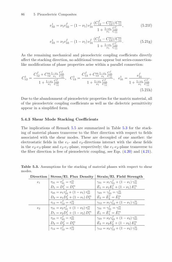
86 5 Piezoelectric Composites
e132 = ν1ef32 − (1 − ν1) ef31
(Cf12 − Cm
12)/Cm11
1 + 1−ν1ν1
Cf11
Cm11
, (5.21f)
e133 = ν1ef33 − (1 − ν1) ef31
(Cf13 − Cm
13)/Cm11
1 + 1−ν1ν1
Cf11
Cm11
. (5.21g)
As the remaining mechanical and piezoelectric coupling coefficients directlyaffect the stacking direction, no additional terms appear but series-connection-like modifications of phase properties arise within a parallel connection:
C112 =
Cf12 + Cm
121−ν1
ν1
Cf11
Cm11
1 + 1−ν1ν1
Cf11
Cm11
, C113 =
Cf13 + Cm
131−ν1
ν1
Cf11
Cm11
1 + 1−ν1ν1
Cf11
Cm11
, e131 =ef31
1 + 1−ν1ν1
Cf11
Cm11
.
(5.21h)
Due to the abandonment of piezoelectric properties for the matrix material, allof the piezoelectric coupling coefficients as well as the dielectric permittivityappear in a simplified form.
5.4.3 Shear Mode Stacking Coefficients
The implications of Remark 5.5 are summarized in Table 5.3 for the stack-ing of material phases transverse to the fiber direction with respect to fieldsassociated with the shear modes. These are decoupled of one another: theelectrostatic fields in the e1- and e2-directions interact with the shear fieldsin the e2-e3-plane and e3-e1-plane, respectively; the e1-e2-plane transverse tothe fiber direction is free of piezoelectric coupling, see Eqs. (4.20) and (4.21).
Table 5.3. Assumptions for the stacking of material phases with respect to shearmodes.
Direction Stress/El. Flux Density Strain/El. Field Strength
e1 τ31 = τf31 = τm
31 γ31 = ν1γf31 + (1 − ν1) γm
31
D1 = Df1 = Dm
1 E1 = ν1Ef1 + (1 − ν1) Em
1
τ23 = ν1τf23 + (1 − ν1) τm
23 γ23 = γf23 = γm
23
D2 = ν1Df2 + (1 − ν1) Dm
2 E2 = Ef2 = Em
2
τ12 = τf12 = τm
12 γ12 = ν1γf12 + (1 − ν1) γm
12
e2 τ31 = ν2τf31 + (1 − ν2) τm
31 γ31 = γf31 = γm
31
D1 = ν2Df1 + (1 − ν2) Dm
1 E1 = Ef1 = Em
1
τ23 = τf23 = τm
23 γ23 = ν2γf23 + (1 − ν2) γm
23
D2 = Df2 = Dm
2 E2 = ν2Ef2 + (1 − ν2) Em
2
τ12 = τf12 = τm
12 γ12 = ν2γf12 + (1 − ν2) γm
12

5.4 Micro-Electromechanics with Sequential Stacking 87
Since the coupled fields have an agreeing direction, they are subjected to thesame kind of assumption of Remark 5.5. Hence, the macroscopic constitutivesubmatrices G
11, G
21, G
12, and G
22, where the upper index is associated with
the stacking direction and the lower with the agreeing direction of the coupledmode, can be determined either directly or via complete inversion from theweighted average:
e1:{τ31D1
}
=(
ν1
(G
f1
)−1
+ (1 − ν1)(G
m1
)−1)−1
︸ ︷︷ ︸G1
1
{γ31E1
}
, (5.22a)
e2:{τ31D1
}
=(ν2G
f1 + (1 − ν2) G
m1
)
︸ ︷︷ ︸G2
1
{γ31E1
}
, (5.22b)
e1:{τ23D2
}
=(ν1G
f2 + (1 − ν1) G
m2
)
︸ ︷︷ ︸G1
2
{γ23E2
}
, (5.22c)
e2:{τ23D2
}
=(
ν2
(G
f2
)−1
+ (1 − ν2)(G
m2
)−1)−1
︸ ︷︷ ︸G2
2
{γ23E2
}
. (5.22d)
The plane transverse to the fiber direction is always involved with the stackingin the considered directions. Thus, for both directions, the macroscopic stresscomponent τ12 of the entirely decoupled shear mode coincides with those ofthe individual phases and the resulting shear stiffnesses C1
66 and C266 only
differ by the participating directional fiber fraction:
e1: τ12 =(
ν1
(Cf
66
)−1
+ (1 − ν1) (Cm66)
−1
)−1
γ12 =Cf
66
ν1(1 + ( 1−ν1ν1
)Cf66
Cm66
)︸ ︷︷ ︸
C166
γ12,
(5.23a)
e2: τ12 =(
ν2
(Cf
66
)−1
+ (1 − ν2) (Cm66)
−1
)−1
γ12 =Cf
66
ν2(1 + ( 1−ν2ν2
)Cf66
Cm66
)︸ ︷︷ ︸
C266
γ12.
(5.23b)
5.4.4 Stacking Sequences
So far, the two necessary cases of stacking of constituents have been examinedfor normal as well as shear modes and macroscopic constitutive relations havebeen obtained for each of them. In the next step, their integration with the goalto depict the simplified representative volume element needs to be considered.

88 5 Piezoelectric Composites
Fig. 5.9. Substitution sequences for the stacking of material phases in the fibercross-sectional plane.
Remark 5.6. The macroscopic properties of the composite may be gained byemploying the effective constitutive coefficients of one stacking direction asinitial constitutive coefficients of the fiber material of the next.
Two possible sequences of these substitutions in the directions of the fibercross-sectional plane arise, as illustrated in Figure 5.9. Thus, the paralleland series connections, as well as combinations thereof, given for instanceby Eqs. (5.21a) to (5.21h), are nested in different ways with in fact diverg-ing results. While Bent and Hagood [15] commit themselves to one of themwithout particular discussion, Tan and Tong [173] interpret the individu-ally distinct coefficients in an extension of the elementary cases consideredin Section 5.3.2 as upper and lower bounds on the effective composite prop-erties. Further insight can be gained with the aid of the following considera-tions.
Remark 5.7. For composites in accordance with Remark 5.2 consisting ofaligned transversely isotropic fiber and matrix materials, the overall materialbehavior is expected to be at most orthotropic and, in the case of identicaldirectional fiber fractions ν1 and ν2, to be transversely isotropic.
When the two stacking sequences are applied to such a configuration withν1 = ν2, in neither case is transversely isotropic material behavior predicted,but both variants show deviations which agree in magnitude but not in axialdirection. Therefore however, their average is consistent with the expectedtransverse isotropy. Thus, the individual stacking sequences sort of introducean artificial degree of orthotropy which may be balanced out by consideringthe combination of both stacking sequences. The two possible stacking se-quences and their combination can be written symbolically with respect to

5.4 Micro-Electromechanics with Sequential Stacking 89
the stacking directions as
1 ⇒ 2, 2 ⇒ 1,⟨
1 ⇒ 22 ⇒ 1
⟩
.
The following fact may be reflected for an illustrative explanation for suchan artificial degree of orthotropy. By substituting the effective constitutivecoefficients of one stacking direction as initial constitutive coefficients of thefiber material of the next, the matrix material is partitioned and subjected todiverging conditions, possibly leading to violations of equilibrium and com-patibility.
5.4.5 Non-Homogeneous Electrostatic Fields
Neither the micro-electromechanical modeling approaches using equivalentinclusions nor the preceding application of the sequential stacking procedureconsider non-homogeneous electrostatic fields. As long as the examined piezo-electric fiber composites are subjected to arbitrary but homogeneous mechan-ical as well as electrostatic fields, these approaches can be applied successfully.While these requirements may be sufficiently fulfilled with the application ofareal electrodes, this is hardly the case when interdigitated electrodes are uti-lized, as illustrated by Figure 5.3. Between electrodes with identical polarityon the top and bottom sides, an inactive zone comes into being, while theactive zone unfolds in the intervals between electrode pairs with opposing po-larity. In between, a transitional region may be identified where, especiallyclose to the electrodes, high field concentrations can be a cause for failureof the composite. For a finite element based analysis of these problems, seeBeckert and Kreher [10].
Stacking in Fiber Direction
A suitable modeling method is sought to capture the losses of actuation andsensing authority due to the imperfect alignment of the electrostatic fieldswith the fiber direction. Relevant parameters are spacing a3 and width b3 ofthe electrodes as well as thickness (a2 − af
2 )/2 and dielectric properties ofthe matrix material between electrode and fiber in addition to the dielectricand piezoelectric properties of the fiber material. As the operative directionof the electrodes is aligned with the polarization direction, the discussion willbe confined to the normal modes. The examination of the simplified repre-sentative volume element with the assistance of the stacking of constituentsin the direction of the fibers is not as obvious as in the previous cases. Ex-amining the implications of Remark 5.5 for the current case, summarized inTable 5.4, in consideration of the fact that the constituents are actually notstacked in this direction and thus the fibers with their superior propertiesclearly dominate the composite’s behavior, suggests assuming the directional

90 5 Piezoelectric Composites
Table 5.4. Assumptions for the stacking of material phases in fiber direction.
Direction Stress/El. Flux Density Strain/El. Field Strength
e3 σ1 = ν3σf1 + (1 − ν3) σm
1 ε1 = εf1 = εm
1
σ2 = ν3σf2 + (1 − ν3) σm
2 ε2 = εf2 = εm
2
σ3 = σf3 = σm
3 ε3 = ν3εf3 + (1 − ν3) εm
3
D3 = Df3 = Dm
3 E3 = ν3Ef3 + (1 − ν3 + c3) Em
3
fiber fraction ν3 = 1. As the lines of electric field strength, sketched in Fig-ure 5.3, not only pass through the fibers in the e3-direction but, in addition,traverse the matrix material, it may be justified to introduce the additionalfactor c3 in conjunction with the electric field strength Em
3 in the matrix ma-terial. In analogy to the considerations of Bent and Hagood [15], the factor c3may be roughly approximated as the share of the matrix material along thelines of the electric field strength on their way through both material phases:
c3 =(a2 − af
2 )
a3 + (a2 − af2 )
=(1 − ν2)
a3a2
+ (1 − ν2). (5.24)
The appearing geometric quantities of the representative volume elementare elucidated in Figure 5.7 and the associated directional fiber fractions aredefined in Eq. (5.1a). In addition to assuming a rectangular path of fieldlines, such an approximation neglects the certainly important electrode widthb3. Thus, it primarily tackles the influences of transitional regions, while theinactive zones are left aside.
Determination of the Stacking Coefficients
To proceed just like in the other stacking cases, the constitutive relation ofEq. (4.19) may be rewritten for fiber and matrix material as follows:
e3:
⎧⎪⎪⎪⎪⎨
⎪⎪⎪⎪⎩
σf1
σf2
εf3
Ef3
⎫⎪⎪⎪⎪⎬
⎪⎪⎪⎪⎭
= Ef3
⎧⎪⎪⎨
⎪⎪⎩
ε1ε2σ3
D3
⎫⎪⎪⎬
⎪⎪⎭
,
⎧⎪⎪⎪⎨
⎪⎪⎪⎩
σm1
σm2
εm3Em
3
⎫⎪⎪⎪⎬
⎪⎪⎪⎭
= Em3
⎧⎪⎪⎨
⎪⎪⎩
ε1ε2σ3
D3
⎫⎪⎪⎬
⎪⎪⎭
. (5.25)
Again, those mechanical and electrostatic fields that originally have been as-sumed to be a weighted average, as stated in Table 5.4, may be arrangedcollectively and Eqs. (5.25) inserted:
e3:
⎧⎪⎪⎨
⎪⎪⎩
σ1
σ2
ε3E3
⎫⎪⎪⎬
⎪⎪⎭
=
⎧⎪⎪⎪⎪⎨
⎪⎪⎪⎪⎩
σf1
σf2
εf3
Ef3
⎫⎪⎪⎪⎪⎬
⎪⎪⎪⎪⎭
+ c3
⎧⎪⎪⎨
⎪⎪⎩
000Em
3
⎫⎪⎪⎬
⎪⎪⎭
=
⎛
⎜⎜⎝E
f3 +
⎡
⎢⎢⎣
0 0 0 00 0 0 00 0 0 00 0 0 c3
⎤
⎥⎥⎦E
m3
⎞
⎟⎟⎠
︸ ︷︷ ︸E3
⎧⎪⎪⎨
⎪⎪⎩
ε1ε2σ3
D3
⎫⎪⎪⎬
⎪⎪⎭
.
(5.26)

5.4 Micro-Electromechanics with Sequential Stacking 91
This still partially inverted macroscopic constitutive relation may be revertedcorrespondingly to the original form of the normal mode constitutive rela-tions:
e3:
⎧⎪⎪⎨
⎪⎪⎩
σ1
σ2
σ3
D3
⎫⎪⎪⎬
⎪⎪⎭
= Cn3
⎧⎪⎪⎨
⎪⎪⎩
ε1ε2ε3E3
⎫⎪⎪⎬
⎪⎪⎭
, with (5.27a)
Cn3 =
⎡
⎢⎢⎢⎢⎢⎢⎢⎢⎢⎢⎣
Cf11 +
(ef31)2
εm33
c3
1+c3εf33
εm33
Cf12 +
ef31e
f32
εm33
c3
1+c3εf33
εm33
Cf13 +
ef31e
f33
εm33
c3
1+c3εf33
εm33
ef31
1+c3εf33
εm33
Cf12 +
ef31e
f32
εm33
c3
1+c3εf33
εm33
Cf22 +
(ef32)2
εm33
c3
1+c3εf33
εm33
Cf23 +
ef32e
f33
εm33
c3
1+c3εf33
εm33
ef32
1+c3εf33
εm33
Cf13 +
ef31e
f33
εm33
c3
1+c3εf33
εm33
Cf23 +
ef32e
f33
εm33
c3
1+c3εf33
εm33
Cf33 +
(ef33)2
εm33
c3
1+c3εf33
εm33
ef33
1+c3εf33
εm33
ef31
1+c3εf33
εm33
ef32
1+c3εf33
εm33
ef33
1+c3εf33
εm33
−εf33
1+c3εf33
εm33
⎤
⎥⎥⎥⎥⎥⎥⎥⎥⎥⎥⎦
.
(5.27b)
Unlike the procedure laid out above, which introduces the factor c3, in thepublications of Bent and Hagood [14,15] and Bent [13], the fraction ν3 is setto one only for the mechanical fields, while it is retained for the electrostaticfields. The resulting constitutive matrix of Eq. (5.27b) therefore becomes non-symmetric with respect to the piezoelectric coupling coefficients. Since theundermost line of the normal mode constitutive relation is not used there anyfurther, this has no consequences.
Discussion of the Stacking Coefficients
As intended, the geometric factor c3 gives rise to the consideration of thedielectric properties of the matrix material. The resulting piezoelectric anddielectric properties are extended in the denominator by the product of thefactor c3 with the ratio of dielectric permittivities of fiber and matrix materialεf33/ε
m33. In comparison to the pure fiber material, these properties therefore
are decreased by a thick matrix layer between fibers and electrodes accordingto the approximation of Eq. (5.24) and by a high dielectric mismatch, which issignificant for the typical materials listed in Tables A.2 and A.3. In both cases,the insulation of the fibers from the electrodes is increased and results in areduction of effectivity of the piezoelectric coupling. The mechanical proper-ties, as they result from the stacking in fiber direction, consist of the stiffnesscoefficients of the fiber material complemented by an additional term, whichrepresents the strengthening due to the piezoelectric effect and again containsthe discussed influence factors.

92 5 Piezoelectric Composites
5.4.6 Stacking Sequences for Non-Homogeneous ElectrostaticFields
Succeeding to the above analysis, the question for the sequence of substitutionsarises again in consideration of two appropriate possibilities. In accordancewith Remark 5.6, either the results of the stacking in the transverse directions,Section 5.4.4, are utilized to represent the fiber phase for the stacking inthe fiber direction, Section 5.4.5, or the other way round. These possibilitiesare illustrated in Figures 5.10(a) and (b), respectively, and may be writtensymbolically as
⟨1 ⇒ 22 ⇒ 1
⟩
⇒ 3 and 3 ⇒⟨
1 ⇒ 22 ⇒ 1
⟩
.
The discussion with regard to the stacking in the fiber direction was boundfor the loss in efficiency of the piezoelectric coupling inherent only to the fibermaterial. Therefore, it may be concluded to begin the substitution sequencewith the e3-direction, as the matrix material otherwise would exert additionalinfluence by means of its share in the preceding stacking cases. Such consider-ations, however, depend on the definition of the factor c3, which needs to berefined requiring detailed experimental studies and finite element simulationswith non-homogeneous polarization. Figure 5.11 exemplarily illustrates theinfluence of the substitution sequence by means of the essential piezoelectric
Fig. 5.10. Over-all substitution sequences for the stacking of material phases.

5.5 Validation of the Micro-Electromechanics 93
Fig. 5.11. Variation of the piezoelectric coupling coefficient e33 with the directionalfiber fractions ν1 and ν2. The values are normalized with respect to the bulk piezo-electric material and homogeneous electrostatic fields. Both substitution sequencesare shown for different factors c3; the results are identical for the homogeneousconditions of c3 = 0.
coupling in the fiber direction. When the coefficients of the stacking in thefiber direction are substituted first, the results have the same character as inthe case of undisturbed electrostatic fields present for a factor c3 = 0. Whenthey are substituted last, distinct deviations are visible which decay with adecreasing factor c3. Further on, the ability of piezoelectric fiber compositesto improve the piezoelectric coupling over the monolithic case of ν1, ν2 = 1may be observed. Finally, it shall be noted that in principle it is also possibleto combine the stacking in the fiber direction to approximate the influenceof non-homogeneous electrostatic fields with any other methodology lackingsuch a capability.
5.5 Validation of the Micro-Electromechanics
In this section, the previously derived micro-electromechanical methodologieswill be validated from the results of experiments as well as finite element mod-els. Such examinations are reported in the literature with adequate topology
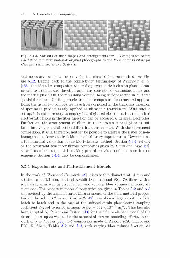
94 5 Piezoelectric Composites
Fig. 5.12. Variants of fiber shapes and arrangements for 1–3 composites beforeinsertation of matrix material; original photographs by the Fraunhofer Institute forCeramic Technologies and Systems.
and necessary completeness only for the class of 1–3 composites, see Fig-ure 5.12. Dating back to the connectivity terminology of Newnham et al.[133], this identifies composites where the piezoelectric inclusion phase is con-nected to itself in one direction and thus consists of continuous fibers andthe matrix phase fills the remaining volume, being self-connected in all threespatial directions. Unlike piezoelectric fiber composites for structural applica-tions, the usual 1–3 composites have fibers oriented in the thickness directionof specimens predominantly applied as ultrasonic transducers. With such aset-up, it is not necessary to employ interdigitated electrodes, but the desiredelectrostatic fields in the fiber direction can be accessed with areal electrodes.Further on, the arrangement of fibers in their cross-sectional plane is uni-form, implying equal directional fiber fractions ν1 = ν2. With the subsequentcomparison, it will, therefore, neither be possible to address the issues of non-homogeneous electrostatic fields nor of arbitrary aspect ratios. Nevertheless,a fundamental validation of the Mori–Tanaka method, Section 5.3.4, relyingon the constraint tensor for fibrous composites given by Dunn and Taya [67],as well as of the sequential stacking procedure with combined substitutionsequence, Section 5.4.4, may be demonstrated.
5.5.1 Experiments and Finite Element Models
In the work of Chan and Unsworth [49], discs with a diameter of 14 mm anda thickness of 1.2 mm, made of Araldit D matrix and PZT 7A fibers with asquare shape as well as arrangement and varying fiber volume fractions, areexamined. The respective material properties are given in Tables A.2 and A.3as provided by the manufacturer. Measurements of the bulk material proper-ties conducted by Chan and Unsworth [49] have shown large variations frombatch to batch and in the case of the induced strain piezoelectric couplingcoefficient d33 led to an adjustment to d33 = 167 × 10−12 m/V. This has alsobeen adopted by Poizat and Sester [143] for their finite element model of thedescribed set-up as well as for the associated current modeling efforts. In thework of Steinhausen [169], 1–3 composites made of Araldit 2020 matrix andPIC 151 fibers, Tables A.2 and A.3, with varying fiber volume fraction are

5.5 Validation of the Micro-Electromechanics 95
examined. For this purpose, fibers with a square shape in a square arrange-ment, with a cylindrical shape in a hexagonal arrangement, as well as witha cylindrical shape in a statistical distribution, have been manufactured, seeFigure 5.12. Unless otherwise indicated, these geometry variants do not showsignificant effects and will not be distinguished in the following. Steinhausen[169] also conducted finite element simulations, which are in good agreementwith the analytical models and will be reproduced here only in uncertaincases.
5.5.2 Dielectric, Piezoelectric, and Mechanical Properties
As mentioned above, the correlation between specified and measured bulkmaterial properties is problematic and further implications will become obvi-ous in the subsequent detailed comparison between experiments and theory.Within the bounds of such variations and of the measurement accuracy, bothrepresentatives of the different micro-electromechanical modeling methodolo-gies can be successfully validated.
Dielectric Properties
The dielectric permittivity εσ33 in the fiber and polarization direction exhibitsa largely linear dependence on the fiber volume fraction ν. In Figures 5.13and 5.14, the Mori–Tanaka method and the sequential stacking procedure de-liver identical results, which agree well with the experimental findings. In thesecond of these figures, slight deviations of the slope may indicate that thematerial data of the constituents is not entirely precise. For the fiber mate-rial, this impression is supported by measured value for ν = 1 being smaller
Fig. 5.13. Variation of the relative di-electric permittivity εσ
33/ε0 with the fibervolume fraction ν; experimental resultsfrom Chan and Unsworth [49].
Fig. 5.14. Variation of the relative di-electric permittivity εσ
33/ε0 with the fibervolume fraction ν; experimental resultsfrom Steinhausen [169].

96 5 Piezoelectric Composites
than the presumed value at the end of the plot of the modeling results. Corre-spondingly, the lower fiber volume fractions point towards a higher dielectricpermittivity of the matrix material.
Piezoelectric Properties
Also for the induced strain piezoelectric coupling coefficient d33 in the fiberand polarization direction, the modeling results cannot be distinguished and,as depicted in Figures 5.15 and 5.16, agree well with the experimental results.While there are some deviations of the experimental data points in the firstof these graphs, the finite element results agree almost perfectly with the an-alytical modeling results. In the second of these graphs, again just a smalldeviation between the fiber properties according to the manufacturer and themeasurement needs to be noted. Experimental investigations of the inducedstrain piezoelectric coupling coefficient d31 have been conducted by Stein-hausen [169]. It is reported that the obvious deviations visible in Figure 5.17are due to surface effects occurring in the experiment, which are not consid-ered in the analytical modelling approaches. Unlike the previously examinedproperties, the coefficient d31 is sensitive to the stacking sequence in the fibercross-sectional plane, and the conformity of the combination of substitutionsequences with Mori–Tanaka as well as the finite element results supports theargumentation of Section 5.4.4.
Fig. 5.15. Variation of the inducedstrain piezoelectric coupling coefficientd33 with the fiber volume fraction ν;experimental results from Chan andUnsworth [49] and finite element resultsfrom Poizat and Sester [143].
Fig. 5.16. Variation of the inducedstrain piezoelectric coupling coefficientd33 with the fiber volume fraction ν;experimental results from Steinhausen[169].
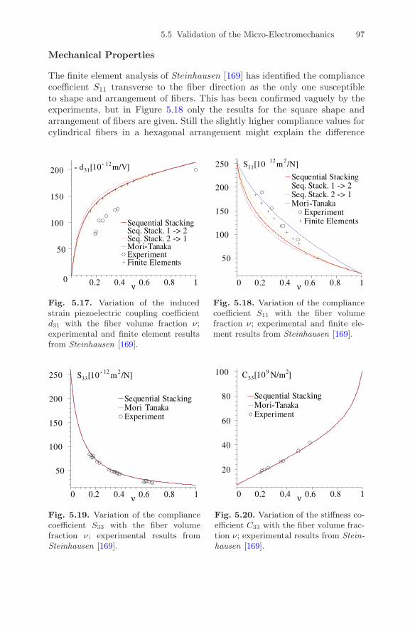
5.5 Validation of the Micro-Electromechanics 97
Mechanical Properties
The finite element analysis of Steinhausen [169] has identified the compliancecoefficient S11 transverse to the fiber direction as the only one susceptibleto shape and arrangement of fibers. This has been confirmed vaguely by theexperiments, but in Figure 5.18 only the results for the square shape andarrangement of fibers are given. Still the slightly higher compliance values forcylindrical fibers in a hexagonal arrangement might explain the difference
Fig. 5.17. Variation of the inducedstrain piezoelectric coupling coefficientd31 with the fiber volume fraction ν;experimental and finite element resultsfrom Steinhausen [169].
Fig. 5.18. Variation of the compliancecoefficient S11 with the fiber volumefraction ν; experimental and finite ele-ment results from Steinhausen [169].
Fig. 5.19. Variation of the compliancecoefficient S33 with the fiber volumefraction ν; experimental results fromSteinhausen [169].
Fig. 5.20. Variation of the stiffness co-efficient C33 with the fiber volume frac-tion ν; experimental results from Stein-hausen [169].

98 5 Piezoelectric Composites
between the Mori–Tanaka method and sequential stacking procedure as theprior emanates from round fibers and the latter from rectangular fibers. Al-together, the accord is less pleasing for this coefficient. Due to requirementsof the measurement technique, Steinhausen [169] used different piezoelectricfibers with inaccurate material data for the determination of the compliancecoefficient S33 in the fiber direction. Therefore, these experiments are com-pared in Figure 5.19 with the analytical models using the original constituentproperties outlined above and yet a good correlation of results is found. Again,the Mori–Tanaka method and sequential stacking procedure lead to indistin-guishable results. This also holds for the stiffness coefficient C33 in the fiberdirection displayed in Figure 5.20.

6
Adaptive Laminated Composite Shells
In this chapter, the transition from voluminous to areal structures, as alreadyprepared in Section 4.4, will be implemented with special regard to laminatedcomposites and adaptive capabilities making use of the piezoelectric effectfor actuation as well as sensing. Therefore, a comprehensive constitutive de-scription is developed and appropriate kinematic relations are specified. After-wards, possibilities of different complexity for the reduction to a less generaldescription are considered in view of specialized application cases.
6.1 Macro-Electromechanics
The examination of the micro-electromechanics in the previous chapter aimedat the homogenized representation of fiber composites with substantial exten-sion in all three dimensions. Within the macro-electromechanics to be con-sidered now, the homogenized representation of laminated composites witha substantial extension only in two dimensions is sought. The graduation interminology alludes to the course of modeling. So laminated fiber compositesfirst pass through the analysis on the micro scale, Section 5.3 or 5.4, and af-ter constitutive reduction, Section 4.4, they enter the analysis on the macroscale.
6.1.1 Lamination Theory
The classical lamination theory, as described by Jones [107] or Whitney [178]for conventional laminates, may be extended to model the assembly of layersor (synonymous) laminae of materials with piezoelectric properties. Here thefollowing will be assumed:
Remark 6.1. The laminate is composed of laminae which are perfectly con-nected by infinitesimally thin and shear resistant bonds.
T.H. Brockmann, Theory of Adaptive Fiber Composites,Solid Mechanics and Its Applications 161,c© Springer Science + Business Media B.V. 2009

100 6 Adaptive Laminated Composite Shells
Further on, for sufficiently thin laminates, the following kinematic assump-tion shall be applicable, usually being denoted as the Kirchhoff–Love hypoth-esis in shell theory:
Remark 6.2. Normal strain and shear strains transverse to the laminate arepresumed to be negligible small.
Regarding a straight line connecting two opposed points on the laminate’sfaces, this assumption implies that under deformation this line conserves itslength and remains straight as well as perpendicular to the laminate’s middlesurface. Such deformations can be expressed by the remaining strains as
⎧⎪⎪⎨
⎪⎪⎩
εxεsγxs
E3
⎫⎪⎪⎬
⎪⎪⎭
=
⎧⎪⎪⎪⎨
⎪⎪⎪⎩
ε0xε0sγ0
xs
E03
⎫⎪⎪⎪⎬
⎪⎪⎪⎭
︸ ︷︷ ︸ε0
+ n
⎧⎪⎪⎨
⎪⎪⎩
κx
κs
ψxs
F3
⎫⎪⎪⎬
⎪⎪⎭
︸ ︷︷ ︸κ
. (6.1)
Initially, the implications of the above assumption will also be adopted todescribe the negated electric field strength E3. Thus, strains as well as electricfield strength are confined to a linear variation through the laminate thicknesswith a constant portion ε0 associated with the middle surface of the laminateand a linear portion nκ. The through thickness coordinate n has its origin atthe middle surface and the gradient is represented by κ. In the case of thestrains, the latter corresponds to the curvatures of the middle surface. Withsuch a collective description of strains and electric field strength across thelayers of the laminate and the individual laminae properties Qk, the stressesand electric flux density of every layer k may be determined as
⎧⎪⎪⎨
⎪⎪⎩
σx
σs
τxs
D3
⎫⎪⎪⎬
⎪⎪⎭k
= Qk
⎧⎪⎪⎨
⎪⎪⎩
εxεsγxs
E3
⎫⎪⎪⎬
⎪⎪⎭
. (6.2)
This equation stems from the general constitutive relation of a thin arbitrarilyoriented lamina given by Eq. (4.31). Stresses and electric flux density of theindividual laminae may be summarized in in-plane resultants N and out-of-plane resultants M by integration over the laminate thickness, in the lattercase, in consideration of the distance to the middle surface:
N =
⎧⎪⎪⎨
⎪⎪⎩
Nx
Ns
Nxs
G3
⎫⎪⎪⎬
⎪⎪⎭
=∫ N/2
−N/2
⎧⎪⎪⎨
⎪⎪⎩
σx
σs
τxs
D3
⎫⎪⎪⎬
⎪⎪⎭k
dn =K∑
k=1
∫ nk
nk−1
⎧⎪⎪⎨
⎪⎪⎩
σx
σs
τxs
D3
⎫⎪⎪⎬
⎪⎪⎭k
dn, (6.3a)
M =
⎧⎪⎪⎨
⎪⎪⎩
Mx
Ms
Mxs
H3
⎫⎪⎪⎬
⎪⎪⎭
=∫ N/2
−N/2
n
⎧⎪⎪⎨
⎪⎪⎩
σx
σs
τxs
D3
⎫⎪⎪⎬
⎪⎪⎭k
dn =K∑
k=1
∫ nk
nk−1
n
⎧⎪⎪⎨
⎪⎪⎩
σx
σs
τxs
D3
⎫⎪⎪⎬
⎪⎪⎭k
dn. (6.3b)

6.1 Macro-Electromechanics 101
Fig. 6.1. Geometry of a laminate with K layers.
The integration over the total laminate thickness N may be replaced by thesum of integrals over the thicknesses nk − nk−1 of each of the altogether Klaminae. The geometry of such a laminate is illustrated in Figure 6.1. Thestresses and electric flux density in Eqs. (6.3) may be substituted with the aidof the laminae constitutive relation of Eq. (6.2), and the collective descriptionof strains and electric field strength with respect to the middle surface may beintroduced by Eq. (6.1). As the latter do not depend on the through thicknesscoordinate n, they can be removed from under the integration and summationsign for the following formulation:
{NM
}
=[A B
B D
]{ε0
κ
}
, (6.4a)
A =K∑
k=1
Qk (nk − nk−1) , B =K∑
k=1
Qk
n2k − n2
k−1
2, D =
K∑
k=1
Qk
n3k − n3
k−1
3.
(6.4b)
6.1.2 Laminates with Groups of Electrically Paralleled Laminae
The above representation is identical to classical lamination theory just thatthe matrix dimensions are extended by virtue of the included electrostaticfields. But the so-far utilized analogous assumptions for the latter need to bethought over, as the effect of the electrodes on the electrostatic field distribu-tion within the individual layer and the parallel connection of electrode pairsof several layers is not yet considered.
Remark 6.3. The electric field strength is assumed to be constant across thethickness of the individual laminae and to be identical in all laminae withparalleled electrode pairs with respect to absolute values.
While a linear through thickness variation of mechanical strains is consid-ered, the electroding by groups of piezoelectric layers results in a piecewise

102 6 Adaptive Laminated Composite Shells
constant distribution of the in-plane electric field strength. Thus, on the onehand the electric field strength gradient F3 introduced in Eq. (6.1) is discardedand therefore also the resultant H3 of Eq. (6.3b) is not required anymore,while on the other hand, the electrostatic fields of electrically connected lami-nae have to be treated separately for every group. Corresponding to Eqs. (6.1)and (6.2), the stresses and electric flux density of layer k belonging to groupg may be expressed in accordance with the above assumption. With the rela-tive sign pk of the electric field strength governed by the electrode connectionwithin the group, this yields
⎧⎪⎪⎨
⎪⎪⎩
σx
σs
τxs
Dg3
⎫⎪⎪⎬
⎪⎪⎭k
= Qk
⎡
⎢⎢⎣
1 0 0 00 1 0 00 0 1 00 0 0 pk
⎤
⎥⎥⎦
⎧⎪⎪⎪⎨
⎪⎪⎪⎩
⎧⎪⎪⎪⎨
⎪⎪⎪⎩
ε0xε0sγ0
xs
Eg3
⎫⎪⎪⎪⎬
⎪⎪⎪⎭
+ n
⎧⎪⎪⎨
⎪⎪⎩
κx
κs
ψxs
0
⎫⎪⎪⎬
⎪⎪⎭
⎫⎪⎪⎪⎬
⎪⎪⎪⎭
with pk ∈ {1,−1} .
(6.5)When the laminate resultants are formed by through thickness integration asin Eqs. (6.3), then the electrostatic fields of every group with connected elec-trodes have to be considered separately. Thus, individual rows and columnsare introduced in the coefficient matrix of the laminate constitutive relation.Explicitly written out for two groups denoted by the letters c and d, theconstitutive relation may be formulated as
⎧⎪⎪⎪⎪⎪⎪⎪⎪⎪⎪⎪⎪⎪⎪⎪⎪⎪⎨
⎪⎪⎪⎪⎪⎪⎪⎪⎪⎪⎪⎪⎪⎪⎪⎪⎪⎩
Nx
Ns
Nxs−Mx
Ms
Mxs−Gc
3
Gd3
...
⎫⎪⎪⎪⎪⎪⎪⎪⎪⎪⎪⎪⎪⎪⎪⎪⎪⎪⎬
⎪⎪⎪⎪⎪⎪⎪⎪⎪⎪⎪⎪⎪⎪⎪⎪⎪⎭
︸ ︷︷ ︸L
=
⎡
⎢⎢⎢⎢⎢⎢⎢⎢⎢⎢⎢⎢⎢⎢⎢⎢⎢⎢⎣
� � � � � � � �A1..3,1..3 B1..3,1..3 Ac
1..3,4 Ad1..3,4 . . .
� � � � � � � � � � � �
B1..3,1..3 D1..3,1..3 Bc1..3,4 Bd
1..3,4 . . .
� � � � �� Ac
1..3,4�T
�� Bc1..3,4
�T
Ac44 0
�� Ad1..3,4
�T
�� Bd1..3,4
�T
0 Ad44
......
. . .
⎤
⎥⎥⎥⎥⎥⎥⎥⎥⎥⎥⎥⎥⎥⎥⎥⎥⎥⎥⎦
︸ ︷︷ ︸K
⎧⎪⎪⎪⎪⎪⎪⎪⎪⎪⎪⎪⎪⎪⎪⎪⎪⎪⎨
⎪⎪⎪⎪⎪⎪⎪⎪⎪⎪⎪⎪⎪⎪⎪⎪⎪⎩
ε0xε0sγ0
xs−κx
κs
ψxs−Ec
3
Ed3
...
⎫⎪⎪⎪⎪⎪⎪⎪⎪⎪⎪⎪⎪⎪⎪⎪⎪⎪⎬
⎪⎪⎪⎪⎪⎪⎪⎪⎪⎪⎪⎪⎪⎪⎪⎪⎪⎭
︸ ︷︷ ︸χ
.
(6.6)The mechanical stiffness coefficients, which are unchanged in comparison tothe classical lamination theory, have been arranged just as they appear inthe latter. They may be determined in accordance with Eqs. (6.4b). As theremaining coefficients are involved with the negated electric field strengthsEg
3 and appertaining resultants Gg3 of the electric flux density, they have to
be established in consideration of the group association represented by the

6.2 Kinematics and Equilibrium 103
functions fgk :
Ag1..4,4 =
K∑
k=1
fgkpk (Q1..4,4)k (nk − nk−1) ,
Bg1..3,4 =
K∑
k=1
fgkpk (Q1..3,4)k
n2k − n2
k−1
2, with fg
k =
{1, k ∈ g,0, k /∈ g.
(6.7)
As there is no electrical connection between the considered groups, the respec-tive coupling coefficients in the constitutive relation, given by Eq. (6.6), haveto be zero. This includes the presumption that the electrodes of a piezoelec-tric layer in general have no influence on other piezoelectric layers, which hasto be guaranteed by the stacking sequence or additional measures. The com-mon theories provide no instruments to collate the electrostatic fields and dowithout resultants of the electric flux density, see Crawley and Lazarus [58],Leibowitz and Vinson [121], or Bent et al. [17]. Thus the resulting constitu-tive description is not compatible to the general form of the energy principles,compare with Eq. (3.63).
6.2 Kinematics and Equilibrium
The strain measures of the laminate have been introduced without specifica-tion of their relation to the displacements field. As the strain measures havebeen established with respect to the middle surface of the laminate, it willalso be the reference for the displacements field.
6.2.1 General Thin Shell Kinematics
To be able to represent arbitrary shapes, the orthogonal curvilinear coordi-nates s1 and s2 on the middle surface are introduced together with the asso-ciated Lame parameters A1 and A2, see for example Dym [69] or Novozhilov[134]. The undeformed middle surface is characterized by the respective prin-cipal radii R1 and R2 in agreement with the following condition:
Remark 6.4. Besides being thin with regard to the overall dimensions, theconsidered shell-like structure is presumed to have a thickness substantiallysmaller than its smallest radius of curvature.
A variety of theories for thin shells are available. For the anticipated ap-plications, it is reasonable to confine the examination to linear theories:
Remark 6.5. The occurring displacements shall be small.
The well-known and generally accepted thin shell theory of Sanders [158]and Koiter [114] eliminated the deficiency of the preceding developments of
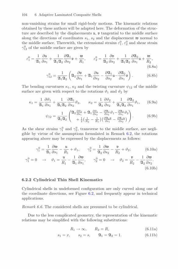
104 6 Adaptive Laminated Composite Shells
non-vanishing strains for small rigid-body motions. The kinematic relationsobtained by these authors will be adapted here. The deformation of the struc-ture are described by the displacements u, v tangential to the middle surfacealong the directions of coordinates s1, s2 and the displacement w normal tothe middle surface. Therewith, the extensional strains ε01, ε
02 and shear strain
γ012 of the middle surface are given by
ε01 =1
A1
∂u
∂s1+
1A1A2
∂A1
∂s2v +
w
R1, ε02 =
1A2
∂v
∂s2+
1A1A2
∂A2
∂s1u +
w
R2,
(6.8a)
γ012 =
1A1A2
(
A2∂v
∂s1+ A1
∂u
∂s2− ∂A1
∂s2u−∂A2
∂s1v
)
. (6.8b)
The bending curvatures κ1, κ2 and the twisting curvature ψ12 of the middlesurface are given with respect to the rotations ϑ1 and ϑ2 by
κ1 =1A1
∂ϑ1
∂s1+
1A1A2
∂A1
∂s2ϑ2, κ2 =
1A2
∂ϑ2
∂s2+
1A1A2
∂A2
∂s1ϑ1, (6.9a)
ψ12 =1
A1A2
(A2
∂ϑ2∂s1
+ A1∂ϑ1∂s2
− ∂A1∂s2ϑ1− ∂A2
∂s1ϑ2
+ 12
(1
R2− 1
R1
)(∂A2v
∂s1− ∂A1u
∂s2
)
)
. (6.9b)
As the shear strains γ01 and γ0
2 , transverse to the middle surface, are negli-gible by virtue of the assumptions formulated in Remark 6.2, the rotationsappearing above may be expressed by the displacements as follows:
γ01 =
1A1
∂w
∂s1− u
R1+ ϑ1, γ0
2 =1
A2
∂w
∂s2− v
R2+ ϑ2; (6.10a)
γ01 = 0 → ϑ1 =
u
R1− 1
A1
∂w
∂s1, γ0
2 = 0 → ϑ2 =v
R2− 1
A2
∂w
∂s2.
(6.10b)
6.2.2 Cylindrical Thin Shell Kinematics
Cylindrical shells in undeformed configuration are only curved along one ofthe coordinate directions, see Figure 6.2, and frequently appear in technicalapplications.
Remark 6.6. The considered shells are presumed to be cylindrical.
Due to the less complicated geometry, the representation of the kinematicrelations may be simplified with the following substitutions:
R1 → ∞, R2 = R, (6.11a)s1 = x, s2 = s, A1 = A2 = 1. (6.11b)

6.2 Kinematics and Equilibrium 105
Fig. 6.2. Orientation of coordinates and displacements for a cylindrical thin shell.
Accordingly, the strain measures as well as rotations have to be renamed.Then the introduction of Eqs. (6.11) into Eqs. (6.8) and (6.9) yields:
ε0x =∂u
∂x, ε0s =
∂v
∂s+
w
R, γ0
xs =∂v
∂x+∂u
∂s, (6.12)
κx =∂ϑx
∂x, κs =
∂ϑs
∂s, ψxs =
∂ϑs
∂x+∂ϑx
∂s+
12R
(∂v
∂x− ∂u
∂s
)
. (6.13)
Similarly the rotations of Eqs. (6.10a) and, consequently, (6.10) reduce to
γ0x =
∂w
∂x+ ϑx, γ0
s =∂w
∂s− v
R+ ϑs, (6.14a)
γ0x = 0 → ϑx = −∂w
∂x, γ0
s = 0 → ϑs =v
R− ∂w
∂s. (6.14b)
and so they can be eliminated from Eqs. (6.13) resulting in
κx = −∂2w
∂x2, κs = −∂
2w
∂s2+∂
∂s
(v
R
), (6.15a)
ψxs = −2∂2w
∂x∂s+∂
∂x
(v
R
)+
12R
(∂v
∂x− ∂u
∂s
)
. (6.15b)
Thus, with Eqs. (6.12) and (6.15), the complete set of strain measures interms of displacements is established for thin cylindrical shells. By neglectingthe underlined terms of Eqs. (6.15), this formulation based on the theoryof Sanders [158] and Koiter [114], may be reduced to the also well-knownformulation of Donnell [64] or Girkmann [84]. Theories similar to the latterlikewise have been developed by Mushtari and Vlasov, see Novozhilov [134].The inspection of the constituents of terms involving the radius shows that

106 6 Adaptive Laminated Composite Shells
derivatives of displacements divided by radius as well as displacements dividedby squared radius are neglected, while displacements divided by radius areretained. As the divergence in the order of magnitude of these ratios increaseswith the radius, such a practice appears to be reasonable, especially for greaterradii of curvature with respect to the shell dimensions. The implications of thesimplifications on the theory for circular cylindrical shells have been discussedextensively in the literature, see Kempner [111], Hoff [99], Simmonds [163],Dym [69].
6.2.3 Cylindrical Thin Shell Equilibrium
The principle of virtual displacements, given by Eq. (3.45), may be utilizedto determine the equations of equilibrium. We will refrain from consideringexternal loads. For the two-dimensional shell structure still with the transverseshear strains γ0
x and γ0s and associated internal transverse forces Qx and Qs,
the principle of virtual displacements may then be reformulated as follows:
δU md =∫∫
Λ
⎧⎪⎪⎪⎪⎪⎪⎪⎪⎪⎪⎪⎪⎨
⎪⎪⎪⎪⎪⎪⎪⎪⎪⎪⎪⎪⎩
δε0x
δε0s
δγ0xs
δκx
δκs
δψxs
δγ0x
δγ0s
⎫⎪⎪⎪⎪⎪⎪⎪⎪⎪⎪⎪⎪⎬
⎪⎪⎪⎪⎪⎪⎪⎪⎪⎪⎪⎪⎭
T ⎧⎪⎪⎪⎪⎪⎪⎪⎪⎪⎪⎨
⎪⎪⎪⎪⎪⎪⎪⎪⎪⎪⎩
Nx
Ns
Nxs
Mx
Ms
Mxs
Qx
Qs
⎫⎪⎪⎪⎪⎪⎪⎪⎪⎪⎪⎬
⎪⎪⎪⎪⎪⎪⎪⎪⎪⎪⎭
dsdx = 0. (6.16)
The virtual strain measures are related to the virtual displacements, just asit is given for the actual case in Eqs. (6.12), (6.13), and (6.14a). When thesekinematic relations are substituted into the principle, different derivativesof the virtual displacements appear. These may be eliminated with the aidof integration by parts to summarize the contributions connected to everyvirtual displacement. In order to satisfy the principle, each of the resultingintegrands needs to vanish. Not to be pursued here, the natural boundary con-ditions therewith can be determined. The sought-after equilibrium conditionsin directions of the coordinates x, s, and n take the following form
∂
∂xNx +
∂
∂sNxs − 1
2∂
∂s
(Mxs
R
)
= 0, (6.17a)
∂
∂sNs +
∂
∂xNxs +
12∂
∂x
(Mxs
R
)
+Qs
R= 0, (6.17b)
∂
∂xQx +
∂
∂sQs − Ns
R= 0, (6.17c)

6.3 Constitutive Reduction 107
while the moment equilibrium conditions about the directions of the coordi-nates x and s read
∂
∂xMx +
∂
∂sMxs − Qx = 0, (6.18a)
∂
∂sMs +
∂
∂xMxs − Qs = 0. (6.18b)
Since the transverse shear strains γ0x and γ0
s will be neglected by virtue ofRemark 6.2, the associated internal transverse forces Qx and Qs may be elim-inated by substitution of Eqs. (6.18) into Eqs. (6.17b) and (6.17c). Thus, theset of equilibrium conditions then consists of Eq. (6.17a) and, considering thatthe radius R of a cylindrical shell is not a function of the coordinate x, of thefollowing:
∂
∂sNs +
∂
∂xNxs +
1R
(32∂
∂xMxs +
∂
∂sMs
)
= 0, (6.19a)
∂2
∂x2Mx + 2
∂2
∂x∂sMxs +
∂2
∂s2Ms − Ns
R= 0. (6.19b)
6.3 Constitutive Reduction
From the mechanical point of view, the theory developed so far allows for theconsideration of adaptive laminated shells subjected to arbitrary loads andstrains within the framework of Remarks 6.1 to 6.6. For many applications,such a level of generality is not necessary as particular knowledge with respectto mission and design may be used to imposed simplifying assumptions.
6.3.1 Negligence of Strain and Stress Components
In the simplest case, certain strain measures are assumed to be negligible andthus the associated column in the matrix of constitutive properties may beeliminated. As the corresponding line in the constitutive relation with regardto the energy contribution is not required either, it can also be removed.In the other case, when an internal force or moment is to be abandoned,the corresponding line in the constitutive relation may be used to determinethe associated strain measure. Substituting the result back into the remaininglines of the constitutive relation leads to an adequate condensation. Analogousprocedures have already been applied in Section 4.4.
Membrane Response
Here the consequences of typical assumptions for the employment of the de-scribed shells as thin walls of a beam will be demonstrated.
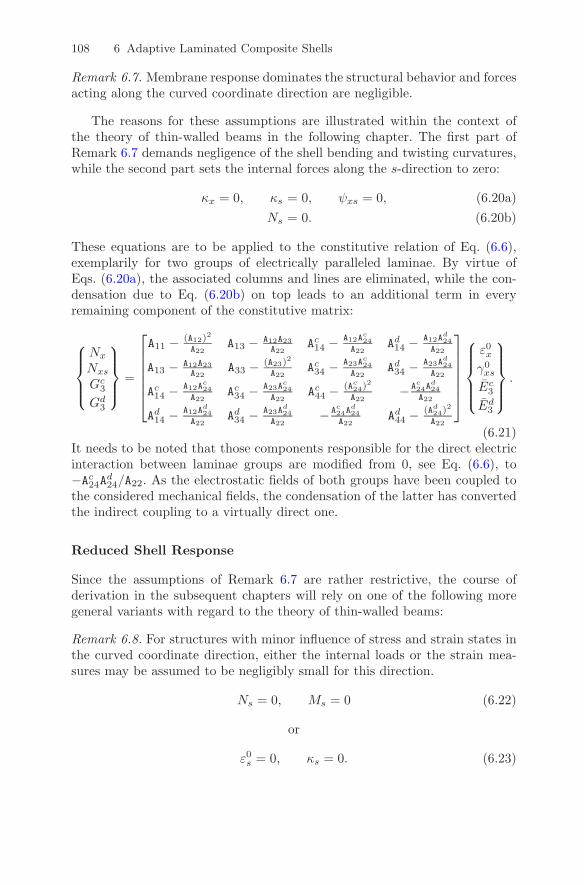
108 6 Adaptive Laminated Composite Shells
Remark 6.7. Membrane response dominates the structural behavior and forcesacting along the curved coordinate direction are negligible.
The reasons for these assumptions are illustrated within the context ofthe theory of thin-walled beams in the following chapter. The first part ofRemark 6.7 demands negligence of the shell bending and twisting curvatures,while the second part sets the internal forces along the s-direction to zero:
κx = 0, κs = 0, ψxs = 0, (6.20a)Ns = 0. (6.20b)
These equations are to be applied to the constitutive relation of Eq. (6.6),exemplarily for two groups of electrically paralleled laminae. By virtue ofEqs. (6.20a), the associated columns and lines are eliminated, while the con-densation due to Eq. (6.20b) on top leads to an additional term in everyremaining component of the constitutive matrix:
⎧⎪⎪⎨
⎪⎪⎩
Nx
Nxs
Gc3
Gd3
⎫⎪⎪⎬
⎪⎪⎭
=
⎡
⎢⎢⎢⎢⎢⎣
A11 − (A12)2
A22A13 − A12A23
A22Ac14 − A12A
c24
A22Ad14 − A12A
d24
A22
A13 − A12A23A22
A33 − (A23)2
A22Ac34 − A23A
c24
A22Ad34 − A23A
d24
A22
Ac14 − A12A
c24
A22Ac34 − A23A
c24
A22Ac44 − (Ac
24)2
A22− Ac
24Ad24
A22
Ad14 − A12A
d24
A22Ad34 − A23A
d24
A22− Ac
24Ad24
A22Ad44 − (Ad
24)2
A22
⎤
⎥⎥⎥⎥⎥⎦
⎧⎪⎪⎪⎨
⎪⎪⎪⎩
ε0xγ0
xs
Ec3
Ed3
⎫⎪⎪⎪⎬
⎪⎪⎪⎭
.
(6.21)It needs to be noted that those components responsible for the direct electricinteraction between laminae groups are modified from 0, see Eq. (6.6), to−Ac
24Ad24/A22. As the electrostatic fields of both groups have been coupled to
the considered mechanical fields, the condensation of the latter has convertedthe indirect coupling to a virtually direct one.
Reduced Shell Response
Since the assumptions of Remark 6.7 are rather restrictive, the course ofderivation in the subsequent chapters will rely on one of the following moregeneral variants with regard to the theory of thin-walled beams:
Remark 6.8. For structures with minor influence of stress and strain states inthe curved coordinate direction, either the internal loads or the strain mea-sures may be assumed to be negligibly small for this direction.
Ns = 0, Ms = 0 (6.22)
or
ε0s = 0, κs = 0. (6.23)

6.3 Constitutive Reduction 109
The negligence of the force Ns and the moment Ms, as of Eq. (6.22), re-quires two condensations to be carried out in analogy to the above discussion.The resulting properties are to be distinguished by the use of (·). The con-densations again lead to non-zero direct electric interaction between laminaegroups symbolized by Acd
44. While the matrix for the reduced shell response isstill symmetric, a loss of symmetry in the off-diagonal submatrices is observedand captured by B31. Consequently, the constitutive relation reads:
⎧⎪⎪⎪⎪⎪⎪⎨
⎪⎪⎪⎪⎪⎪⎩
Nx
Nxs
Mx
Mxs
Gc3
Gd3
⎫⎪⎪⎪⎪⎪⎪⎬
⎪⎪⎪⎪⎪⎪⎭
=
⎡
⎢⎢⎢⎢⎢⎢⎢⎣
A11 A13 B11 B13 Ac14 Ad
14
A13 A33 B31 B33 Ac34 Ad
34
B11 B31 D11 D13 Bc14 Bd
14
B13 B33 D13 D33 Bc34 Bd
34
Ac14 Ac
34 Bc14 Bc
34 Ac44 Acd
44
Ad14 Ad
34 Bd14 Bd
34 Acd44 Ad
44
⎤
⎥⎥⎥⎥⎥⎥⎥⎦
⎧⎪⎪⎪⎪⎪⎪⎪⎨
⎪⎪⎪⎪⎪⎪⎪⎩
ε0xγ0
xs
κx
ψxs
Ec3
Ed3
⎫⎪⎪⎪⎪⎪⎪⎪⎬
⎪⎪⎪⎪⎪⎪⎪⎭
. (6.24)
Neglecting strain ε0s and curvature κs, as of Eq. (6.23), allows us to deletethe associated columns and rows of the matrix, respectively, vectors in theoriginal constitutive relation of Eq. (6.6). However, Eq. (6.24) may be used torepresent both cases of the reduced shell response, since the latter is includedas a special case:
(·) = (·) with B31 = B13 = B13 and Acd44 = 0. (6.25)
6.3.2 Potential Energy Considerations
Another possibility to reduce the number of components in the constitutiverelation of adaptive laminated shells is to employ the extended Dirichlet’sprinciple of minimum potential energy derived in Section 3.5.1.
Remark 6.9. External mechanical loads, as well as external electric charges,will be confined to minor changes in comparison to the internal states.
Therefore, the minimization is not affected by these external influencesand, consequently, Eq. (3.69) reduces to
U ⇒ min . (6.26)
With the preceding constitutive modeling, the associated electroelastic energydensity U0, see Eq. (3.65), may now be given for adaptive laminated shells as
U0 =12χT
Kχ with K = KT , (6.27a)
=12χT
Kχ + χTKχ +
12χT
Kχ, K = KT , K = K
T . (6.27b)

110 6 Adaptive Laminated Composite Shells
Here the considerations of Section 4.4.4 again warrant the symmetry of thelaminate constitutive matrix K, introduced in Eq. (6.6), together with the vec-tor χ consisting of shell strains and groupwise electric field strengths. Equa-tion (6.27a) may be rewritten for an arbitrary rearrangement of the compo-nents of χ in the vectors χ and χ with the corresponding property matricesK, K, and K as given by Eq. (6.27b). For such a partitioning, the constitutiverelation of Eq. (6.6) with the vector L of shell internal loads and groupwiseelectric flux density resultants reorganized in the vectors L and L reads asfollows: {
LL
}
=[
K K
KT
K
]{χχ
}
. (6.28)
Constrained Variational Problem of Several Independent Variables
In the first instance, the general formulation of such a problem shall be con-sidered. As the expression U0 is a function of functions, in the current casecontained in the vector χ, it is denoted as functional. The functions andthus the functional may depend on several mutually independent variables,whereby, without loss of generality, the two-dimensional case will be exam-ined. Correspondingly, the appearance of first derivatives of the functions isincorporated. The extremum of the integral
U =∫ x1
x0
∫ s1
s0
U0(x, s,χ(x, s),χ,x(x, s),χ,s(x, s)) dsdx (6.29)
is sought after. The functions contained in the vector χ will be subjected toan arbitrary number of side conditions. These constraints are of the followingform:
∫ x1
x0
∫ s1
s0
ς(x, s,χ(x, s)) dsdx = c, (6.30a)∫ x1
x0
ς(x, s,χ(x, s)) dx = c (s) ,∫ s1
s0
ς(x, s,χ(x, s)) ds = c (x) , (6.30b)
ς(x, s,χ(x, s),χ,x(x, s),χ,s(x, s)
)= 0. (6.30c)
Euler’s differential equations in conjunction with the introduction of La-grangian multipliers constitute the necessary conditions for a minimum, seeCourant and Hilbert [56] or Denn [62]. Thereby the integrand U0 of Eq. (6.29)is extended by the product of appropriate parameters known as Lagrangianmultipliers and integrands of the side conditions. In the vectorial representa-tion to be given here, this results in U0 + λT ς with the vector of Lagrangianmultipliers λ and respective vector of integrands ς from Eqs. (6.30). To ob-tain Euler’s differential equations, the variation of this expression is equatedto zero:
∂
∂s
∂
∂χ,s
(U0 + λT ς
)+∂
∂x
∂
∂χ,x
(U0 + λT ς
)− ∂
∂χ
(U0 + λT ς
)= 0. (6.31)

6.3 Constitutive Reduction 111
To determine the Lagrangian multipliers, the side conditions have to be con-sulted. The different types of side conditions given in Eqs. (6.30), identifythe dependencies of the Lagrangian multipliers. In the case of Eq. (6.30a),it is dealt with a constant, while for Eqs. (6.30b) the Lagrangian multipliersdepend on the variables s, respectively x. Consequently in the general caseof Eq. (6.30c), the Lagrangian multipliers are functions of all independentvariables. For a sophisticated discussion of the sufficient conditions for a min-imum in the calculus of variations, see the pertinent literature, for exampleFunk [77].
Actual Problem
Inspecting Eqs. (6.27), it is found that the actual problem at hand is signif-icantly simpler and can be deduced from the above implementations. As thegoal was to reduce the number of components in the constitutive relation,the vector χ may be subdivided, see Eq. (6.27b), into a portion χ to be re-tained and a portion χ to be expressed in terms of the prior. This can beaccomplished by minimizing the electroelastic energy U with respect to thefunctions contained in the vector χ:
U =∫ x1
x0
∫ s1
s0
U0(x, s, χ(x, s)) dsdx. (6.32)
The minimization with respect to a subset of functions is permissible insofaras the examination of a subset of Euler’s differential equations has no limitingimplications on an eventually succeeding complete solution of the problem.The imposed side conditions will be given in the form of the right-hand sideof Eqs. (6.30b) and are supposed to be linear with respect to the vector χinvolving a proportionality matrix Γ:
∫ s1
s0
Γ(x, s) χ(x, s) ds = c (x) . (6.33)
Thus, for the problem at hand, Euler’s differential equations, given in generalform by Eq. (6.31), reduce to
∂
∂χ
(U0 + λT Γχ
)= 0. (6.34)
Solving Eq. (6.34) in consideration of the electroelastic energy density U0 asgiven by Eq. (6.27b) for the vector χ, it can be established in terms of thevectors χ and λ:
χ = −K−1
KT χ − K
−1ΓT λ. (6.35)
Finally, the Lagrangian multipliers have to be determined by substitution ofEq. (6.35) into Eq. (6.33). The associated vector λ can be easily isolated as

112 6 Adaptive Laminated Composite Shells
it does not depend on the integration variable s:
λ = −∫ s1
s0
(ΓK
−1ΓT)−1
ds(
c +∫ s1
s0
ΓK−1
KT χ ds
)
. (6.36)
Congeneric findings are reported by Volovoi and Hodges [176] for the solelymechanical case. As noted there, similarities to a procedure applied by Reiss-ner and Tsai [152] exist involving the partial inversion of the constitutiverelation. Such an approach is also found in further works by Reissner [151],Murakami et al. [129], and Jung et al. [108].
Implications of the Potential Energy Minimization
The operating characteristics of the elaborated procedure may be recalled inthe following statement:
Remark 6.10. The eliminated set of components adjusts such that the poten-tial energy is minimal for the remaining set of components being assumed asgiven.
Simplifications tied to already eliminated components cannot be appliedanymore. Therefore, such constraints have to be considered during the min-imization with aid of the Lagrangian multipliers. To assess further conse-quences of the partial minimization, the result of Eq. (6.35) is substitutedinto the associated constitutive relation of Eq. (6.28). After a couple of re-arrangements, this yields
{LL
}
=
[
K − KK−1
KT
0
]
χ −[
KK−1
I
]
ΓT λ. (6.37)
Examining the lower part of Eq. (6.37), it is observed that the shell inter-nal loads and groupwise electric flux density resultants in the vector L onlydepend on the constraint contributions ΓT λ and thus directly reveal the im-plications of the minimization. Due to the integral form of the regarded sideconditions, given by Eq. (6.33), the Lagrangian multipliers in the vector λ rep-resent elements of internal loads or flux density resultants that are constantalong the s-direction. In the case of components to be eliminated without theexistence of associated side conditions, the constraint contributions vanish asa matter of course and the following can be concluded:
Remark 6.11. Minimization with respect to unconstrained components isequivalent to neglecting the corresponding internal loads or groupwise electricflux density resultants respectively.
Examining the upper part of Eq. (6.37), the shell internal loads and group-wise electric flux density resultants in the vector L are found to be composed

6.3 Constitutive Reduction 113
of two parts. The second of them again represents the constraint contribu-tions just that the adjustment KK
−1is incorporated here. The first part is
a function of the retained shell strains and groupwise electric field strengthsin the vector χ depending on both the coordinates x and s. The submatrixK is complemented by an additional term. It contains the transposed subma-trix K, originally responsible for the coupling with the eliminated vector χ,in conjunction with the above-mentioned adjustment KK
−1. As suggested by
Remark 6.11, the additional term agrees with the corresponding findings ofSection 6.3.1.
Example
To illustrate the above procedure, at least the set up of a typical problem willbe given. Therein it is dealt with a single-cell closed cross-section beam andthe associated kinematic constraints. Again for the theoretical backgroundand information on the appearing quantities, we will refer to the subsequentchapter. The vectors and matrices to be inserted into Eqs. (6.36) and (6.37)are
χ =
⎧⎪⎪⎪⎪⎨
⎪⎪⎪⎪⎩
ε0xκx
ψxs
Ec3
Ed3
⎫⎪⎪⎪⎪⎬
⎪⎪⎪⎪⎭
, χ =
⎧⎨
⎩
ε0sγ0
xs
κs
⎫⎬
⎭, Γ =
⎡
⎢⎢⎣
0 1 00 0 10 0 y0 0 z
⎤
⎥⎥⎦ ,
(6.38a)
c =
⎧⎪⎪⎪⎨
⎪⎪⎪⎩
∂φ∂x
∮
S
rn ds
000
⎫⎪⎪⎪⎬
⎪⎪⎪⎭
, λ =
⎧⎪⎪⎨
⎪⎪⎩
λ1
λ2
λ3
λ4
⎫⎪⎪⎬
⎪⎪⎭
,
K =
⎡
⎢⎢⎢⎢⎢⎣
A11 B11 B13 Ac14 Ad
14
B11 D11 D13 Bc14 Bd
14
B13 D13 D33 Bc34 Bd
34
Ac14 Bc
14 Bc34 Ac
44 0Ad14 Bd
14 Bd34 0 Ad
44
⎤
⎥⎥⎥⎥⎥⎦
, K =
⎡
⎢⎢⎢⎢⎣
A12 A13 B12
B12 B13 D12
B23 B33 D23
Ac24 Ac
34 Bc24
Ad24 Ad
34 Bd24
⎤
⎥⎥⎥⎥⎦
,
(6.38b)
K =
⎡
⎣A22 A23 B22
A23 A33 B23
B22 B23 D22
⎤
⎦ .
By substitution of Γ, χ, and c from Eq. (6.38a) into the side condition ofEq. (6.33) it becomes clear that the strain ε0s is unconstrained and thus theinternal force Ns is neglected. Further on, the integral of the shear strain γ0
xs
is equated to a function of x, while in the case of the bending curvature κs,it is the constant zero.

7
Adaptive Thin-Walled Beams
Based upon the adaptive shell description given in the previous chapter, athin-walled beam formulation for general anisotropic cross-sections with arbi-trary open branches and/or closed cells will be derived in this chapter. Afterthe deduction of non-linear kinematic relations for the general beam and thelinear kinematic relations for the thin-walled beam, the torsional warping ef-fects of the latter are examined. Subsequently, the constitutive relation andthe equations of equilibrium are established.
7.1 General Beam Kinematics
With regard to the dynamics of rotating structures on the one hand, non-linear influences in the beam kinematics have to be taken into account, whileanalytical formulation of the constitutive relation of beams with complicatedcross-sections on the other hand, is only possible for thin walls and linearkinematics. This gives rise to a combined procedure with a linear analysisto determine the beam properties and a succeeding non-linear analysis toinvestigate the global beam behavior. For the latter, a general beam withadequate kinematics will be examined first and subsequently transcribed intothe intended thin-walled beams.
7.1.1 Positions and Displacements
Like in the case of the shell in Section 6.2, the displacement field needs to bespecified for the beam as well. Since the course of analysis will lead to rotatingbeams, which rather do without curvature, we will agree on the following:
Remark 7.1. The beam will be prismatic with unvarying cross-sectional prop-erties along a reference line which is straight in the initial state.
The coordinate x accounts for the essential dimension of the beam andinitially coincides with its reference line, while the orthogonal coordinates y
T.H. Brockmann, Theory of Adaptive Fiber Composites,Solid Mechanics and Its Applications 161,c© Springer Science + Business Media B.V. 2009

116 7 Adaptive Thin-Walled Beams
and z characterize the transverse plane. In this reference system, the posi-tion P o(x, y, z) of an arbitrary point within the undeformed beam may bedescribed by
P o (x, y, z) = xo (x) + so (y, z) with xo (x) =
⎧⎨
⎩
x00
⎫⎬
⎭, so (y, z) =
⎧⎨
⎩
0yz
⎫⎬
⎭.
(7.1)The intersection point of the cross-sectional plane with the beam referenceline will be called the reference point. In the initial state, the vector xo(x)marks this reference point, while the vector so(y, z) specifies the position ofthe considered point on the cross-sectional plane. Consequently, its positionpo(x, y, z) in the deformed state can be given with the aid of the total dis-placement uo(x, y, z) as
po (x, y, z) = P o (x, y, z) + uo (x, y, z) . (7.2)
We will start with a geometrically exact specification of the total displacement.Here a separation of displacements with respect to the reference line and cross-section is utilized. Thus, the displacement of the reference point is expressedby the vector u(x), while the remaining terms account for the displacementassociated with the cross-section:
uo (x, y, z) = u (x) + R (x) (so (y, z) + uΘ (x, y, z)) − so (y, z)
with u (x) =
⎧⎨
⎩
u (x)v (x)w (x)
⎫⎬
⎭, uΘ (x, y, z) =
⎧⎨
⎩
uΘ (x, y, z)vΘ (x, y, z)wΘ (x, y, z)
⎫⎬
⎭. (7.3)
The vector uΘ(x, y, z) contains the displacements due to the deformation ofthe cross-section usually entitled “warping”. Together with the vector so(y, z),it describes the position relative to the reference point sitting on the now-deformed reference line requiring the rotational transformation R(x) to com-ply with the reference system. To gain the displacement portion, the cross-sectional position in the initial state so(y, z) needs to be subtracted.
7.1.2 Rotations
There are a number of possibilities including Euler angles and quaternionsto express finite rotations in three dimensions, see Gerardin and Rixen [80].To avoid a dependency on the sequence of three separate transformations, asencountered for example by Hodges and Dowell [98] or Kaza and Kvaternik[110], the angular coordinates of Rodriguez can be utilized, see Gasch andKnothe [78] or Sauer [159]. Therewith the transformation matrix R(x) canbe formulated as
R (x) = I +sinββ
〈β (x)〉 +1 − cosββ2
〈β (x)〉2 with β = β (x) = ‖β (x)‖ .
(7.4)

7.1 General Beam Kinematics 117
This contains the rotational angle β(x) and the skew-symmetric matrix〈β(x)〉, defined in Eq. (3.9), whereby both are associated with the vectorβ(x) of rotational parameters. In the cases of moderate or small rotations,the latter turn into the rotational angles around the axes of the referencesystem:
β (x) =
⎧⎨
⎩
φ (x)βy (x)βz (x)
⎫⎬
⎭. (7.5)
For moderate rotations, Eq. (7.6a), and small rotations, Eq. (7.6b), the Ro-driguez formula of Eq. (7.4) reduces as follows:
sinβ = β, cosβ = 1 − β2
2→ R (x) = I + 〈β (x)〉 +
12
〈β (x)〉2 , (7.6a)
sinβ = β, cosβ = 1 → R (x) = I + 〈β (x)〉 . (7.6b)
Thus, for small rotations only the sum of the identity matrix and skew-symmetric matrix remains. In any case, such rotational transformations shallbe reversible and therefore orthogonality is required:
R (x)T R (x) = I. (7.7)
The substitution of the simplified transformation matrices of Eqs. (7.6) intothis condition reveals those terms which have been neglected by the associ-ated assumptions. In the case of moderate rotations, Eq. (7.6a), and smallrotations, Eq. (7.6b), these are the products of four, respectively of two, ro-tational angles given in Eq. (7.5). Since the rotational angles in the lattercase are thereby decoupled, the outcome is identical to the results of otherrotational transformations, for example involving Euler angles.
7.1.3 Simplifications
The geometrically exact specification of displacements not unexpectedly leadsto fairly complicated expressions, and also for moderate rotations, it is usu-ally sought after reduction with the aid of ordering schemes. For the sake oftransparency and analytic insight, it will be continued as follows:
Remark 7.2. The beam may be subjected only to small rotations.
Applying the rotational transformation for such small rotations, as out-lined in Eq. (7.6b), to the total displacement vector uo(x, y, z) of Eq. (7.3)leads to
uo (x, y, z) = u (x) + (I + 〈β (x)〉) (so (y, z) + uΘ (x, y, z)) − so (y, z) . (7.8)
So far, the warping displacements uΘ(x, y, z) have not been considered beyondtheir pure existence. Yet, they somehow must be related to the displacementsu(x) or rotations β(x) of the beam. A detailed analysis of the warping effectswill be given later in this chapter, illustrating the subsequent warping-relatedstatements.

118 7 Adaptive Thin-Walled Beams
Remark 7.3. The warping displacements are presumed to be functions of therotational angles.
Therefore, the multiplication of the skew-symmetric matrix 〈β(x)〉 withthe warping displacements uΘ(x, y, z) in Eq. (7.8) results in products of twoangles or derivatives thereof respectively. In consequence of the above discus-sion on the orthogonality condition, these terms have to be neglected and theexpression of the total displacements simplifies significantly:
uo (x, y, z) = u (x) + β (x) × so (y, z) + uΘ (x, y, z) . (7.9)
The deformation of the cross-section is considered to be subdivided intothe out-of-plane warping uΘ(x, y, z) and the in-plane warping vΘ(x, y, z),wΘ(x, y, z). The latter is neglected with the introduction of a classical as-sumption of beam theory:
Remark 7.4. The cross-section remains undeformed in its plane.
vΘ (x, y, z) = 0, wΘ (x, y, z) = 0. (7.10)
For the thin-walled beams to be subsequently discussed, this is a fairlyrough assumption since the bending stiffness of their walls might be com-parably low. Some approaches are reported in the literature to incorporatethe in-plane deformation of the cross-section, see Heo et al. [93], Rand [148],or Rand [149], but in return have to accept other limitations or drawbacks.Concentrating on the out-of-plane warping here and in anticipation of the de-tailed discussion in Section 7.3, the associated displacement component maybe described by
uΘ (x, y, z) = Θ (y, z)φ,x (x) . (7.11)
Therein the warping function Θ(y, z) accounts for the cross-sectional proper-ties, while the lengthwise dependency is provided by the rate of twist φ,x(x).Supplying Eq. (7.9) with Eq. (7.11), the components of the total displacementof the classic beam theory of Euler and Bernoulli with extension to shear flexi-bility and torsional warping usually associated with the names of Timoshenko,respectively Vlassov, are obtained:
uo (x, y, z) =
⎧⎨
⎩
u0 (x, y, z)v0 (x, y, z)w0 (x, y, z)
⎫⎬
⎭
=
⎧⎨
⎩
u (x) + zβy (x) − yβz (x) +Θ (y, z)φ,x (x)v (x) − zφ (x)w (x) + yφ (x)
⎫⎬
⎭. (7.12)
Due to the elongated nature of beams in general, their resistance againstextension is drastically higher than against bending. Correspondingly, thedisplacement u(x) in the axial direction in almost any case is significantlysmaller than the displacements v(x), w(x) in the transverse directions. Hence,the following may be concluded:

7.1 General Beam Kinematics 119
Remark 7.5. The beam may be subjected to finite displacements, whereof thedisplacement in the axial direction may be considered as moderate withoutloss of generality.
7.1.4 Strains
In order to determine the strain measures of the general beam, the GreenLagrange strain tensor for finite deformations may be utilized as outlined inSection 3.2.4. It is symmetric and contains, in general, six independent com-ponents, to be obtained from Eq. (3.17) for the total displacements u0(x, y, z).However, due to the assumption of Remark 7.4, both normal strains and theshear strain in the cross-sectional plane have to vanish. So the remainingcomponents are the normal strain as well as the two shear strains associatedwith lengthwise direction. Resorting them into a vector in consideration ofthe factor for the engineering shear strains, yields
εGL(x, y, z) =
⎧⎪⎪⎨
⎪⎪⎩
∂∂xu0 + 1
2 ( ∂∂xu0)2 + 1
2 ( ∂∂xv0)
2 + 12 ( ∂
∂xw0)2
∂∂xv0 + ∂
∂yu0 + ∂∂xu0
∂∂yu0 + ∂
∂xv0∂∂y v0 + ∂
∂xw0∂∂yw0
∂∂xw0 + ∂
∂zu0 + ∂∂xu0
∂∂zu0 + ∂
∂xv0∂∂z v0 + ∂
∂xw0∂∂zw0
⎫⎪⎪⎬
⎪⎪⎭
.
(7.13)Next, the components of the total displacement as given by Eq. (7.12) maybe substituted into Eq. (7.13). In consideration of Remark 7.5, the derivativeof the axial displacement may be neglected in comparison to unity:
1 + u,x (x) ≈ 1. (7.14)
Thus, as well as with the abandonment of any product of two rotational anglesby virtue of Remark 7.2, the remaining Green Lagrange strain componentsmay be significantly simplified. Arranging the non-linear strain measures forfinite displacements but small rotations of the beam in the vector εGL(x),leads to
εGL (x, y, z)
=
[1 0 0 0 z −y Θ (y, z)0 1 0 Θ,y (y, z) − z 0 0 0
0 0 1 Θ,z (y, z) + y 0 0 0
]
⎧⎪⎪⎪⎪⎪⎪⎨
⎪⎪⎪⎪⎪⎪⎩
u,x(x) + 12(v,x(x)2 + w,x(x)2)
−βz (x) + v,x (x) + w,x (x) φ (x)
βy (x) + w,x (x) − v,x (x) φ (x)
φ,x (x)
βy,x (x) − v,x (x) φ,x (x)
βz,x (x) − w,x (x) φ,x (x)
φ,xx (x)
⎫⎪⎪⎪⎪⎪⎪⎬
⎪⎪⎪⎪⎪⎪⎭
︸ ︷︷ ︸εGL(x)
.
(7.15)
Analogous treatment of those Green Lagrange strain components, which areexpected to vanish as discussed above, reveals only terms with products of tworotational angles. These again have to be neglected by virtue of Remark 7.2,and so the implications of Remark 7.4 are confirmed.

120 7 Adaptive Thin-Walled Beams
7.2 Thin-Walled Beam Kinematics
So far, the shape of the cross-section of the considered beams has not beendiscussed, while the Green Lagrange strain tensor has been brought up fora continuum only confined with respect to the deformations in the cross-sectional plane by Remark 7.4. Subsequently, a special class of cross-sectionaltopologies will be examined:
Remark 7.6. The beam is constructed from walls which are thin in comparisonto the cross-sectional dimensions.
Under these conditions, it is possible to analytically handle beams withcomplex cross-sections, since the formation of the one-dimensional structurefrom two-dimensional walls instead of a three-dimensional continuum allowsus to introduce the associated simplifications. Therefore, the relation betweenthe strain measures of the beam and of the thin wall is sought. To describethe shape of such a cross-section, the curvilinear coordinate s may be utilizedas a parameter for the cross-sectional position
so (y, z) =
⎧⎨
⎩
0yz
⎫⎬
⎭=
⎧⎨
⎩
0y (s)z (s)
⎫⎬
⎭= so (s) . (7.16)
Correspondingly, the above derivations may be adjusted to account for thecoordinate s in the cross-sectional plane.
7.2.1 Differential Geometry
The curvilinear coordinate s will be given such that it represents the arc lengthand therefore, just as in the case of the Lame parameters for the cylindricalshell in Section 6.2.2, the following is required:
∣∣∣∣∂
∂sso(s)
∣∣∣∣ =
√
(y,s(s))2 + (z,s(s))
2 = 1. (7.17)
The unit tangent vector es(s) is given by the corresponding derivative of thecross-sectional position so(s). Further on, the unit normal vector en(s) isdefined orthogonal to the unit axis vector ex in parallel to the undeformedreference line and to the unit tangent vector es(s). Thus, the moving trihedralis given as
ex =
⎧⎨
⎩
100
⎫⎬
⎭, es(s) =
∂∂sso(s)
| ∂∂sso(s)|
=
⎧⎨
⎩
0y,s(s)z,s(s)
⎫⎬
⎭, (7.18a)
en (s) = ex × es (s) =
⎧⎨
⎩
0−z,s(s)y,s(s)
⎫⎬
⎭. (7.18b)

7.2 Thin-Walled Beam Kinematics 121
In the description of spatial curves or surfaces, the radius of curvature isusually an absolute value and the direction of curvature is given by the unitprincipal normal vector, pointing towards the center of curvature. Then theunit binormal vector results from the vector product of unit tangential andunit principal normal vector, see Rade and Westgren [147] or Wygodski [185].Instead, here the unit axis vector ex needs to be prearranged just as the unittangent vector es(s) and thus, for the sake of orthogonality, the unit normalvector en(s) is not necessarily oriented towards the center of the curvature,while the radius R(s) may then also become negative. The sequence of spatialdirections in the wall description (x, s, n) has been chosen in Eq. (7.18b) tobegin with the coincidental coordinate x, as appears in the beam description(x, y, z). For this reason, a positive radius R(s) is now associated with anoutward oriented unit normal vector en(s), as visible in Figure 7.1, and anegative sign needs to be introduced into the corresponding relation:
−en (s) =∂2
∂s2so(s)R (s) . (7.19)
With Eqs. (7.16) and (7.18), this relations allows us to express the radius R(s)in terms of the cross-sectional position:
R (s) = − y,s(s)z,ss(s)
=z,s(s)y,ss(s)
. (7.20)
Fig. 7.1. Position of a point on the cross-section and associated unit vectors.
7.2.2 Cartesian and Curvilinear Positions and Displacements
To transform vector-valued functions from the Cartesian coordinate systemof the beam to the curvilinear coordinate system of the wall, the unit vec-
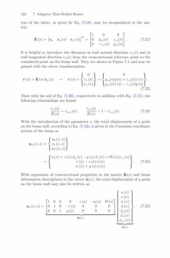
122 7 Adaptive Thin-Walled Beams
tors of the latter, as given by Eq. (7.18), may be encapsulated in the ma-trix
E (s) =[ex es (s) en (s)
]T =
⎡
⎣1 0 00 y,s(s) z,s(s)0 −z,s(s) y,s(s)
⎤
⎦ . (7.21)
It is helpful to introduce the distances in wall normal direction rn(s) and inwall tangential direction rs(s) from the cross-sectional reference point to theconsidered point on the beam wall. They are shown in Figure 7.1 and may begained with the above transformation:
r (s) = E (s) so (s) → r (s) =
⎧⎨
⎩
0rs (s)rn (s)
⎫⎬
⎭=
⎧⎨
⎩
0y,s(s)y (s) + z,s(s)z (s)y,s(s)z (s) − z,s(s)y (s)
⎫⎬
⎭.
(7.22)
Then with the aid of Eq. (7.20), respectively in addition with Eq. (7.17), thefollowing relationships are found:
rs (s)R (s)
= rn,s (s) ,rn (s)R (s)
= 1 − rs,s (s) . (7.23)
With the introduction of the parameter s, the total displacement of a pointon the beam wall, according to Eq. (7.12), is given in the Cartesian coordinatesystem of the beam as
uo (x, s) =
⎧⎨
⎩
u0 (x, s)v0 (x, s)w0 (x, s)
⎫⎬
⎭
=
⎧⎨
⎩
u (x) + z (s)βy (x) − y (s)βz (x) +Θ (s)φ,x (x)v (x) − z (s)φ (x)w (x) + y (s)φ (x)
⎫⎬
⎭. (7.24)
With separation of cross-sectional properties in the matrix K(s) and beamdeformation descriptions in the vector u(x), the total displacement of a pointon the beam wall may also be written as
uo (x, s) =
⎡
⎣1 0 0 0 z (s) −y (s) Θ (s)0 1 0 −z (s) 0 0 00 0 1 y (s) 0 0 0
⎤
⎦
︸ ︷︷ ︸K(s)
⎧⎪⎪⎪⎪⎪⎪⎪⎪⎨
⎪⎪⎪⎪⎪⎪⎪⎪⎩
u (x)v (x)w (x)φ (x)βy (x)βz (x)φ,x (x)
⎫⎪⎪⎪⎪⎪⎪⎪⎪⎬
⎪⎪⎪⎪⎪⎪⎪⎪⎭
︸ ︷︷ ︸u(x)
. (7.25)

7.2 Thin-Walled Beam Kinematics 123
To determine the strains in the beam wall, the total displacement must beexpressed in the associated curvilinear coordinate system. With the aid of thetransformation of Eq. (7.21), this may be expressed in the following form:
⎧⎨
⎩
u (x, s)v (x, s)w (x, s)
⎫⎬
⎭= E (s) uo(x, s). (7.26)
7.2.3 Strains of Wall and Beam
Since the thin walls of the prismatic beams under discussion resemble thecylindrical thin shells of Section 6.2.2, the associated formulation of strainsmay be adopted. Thereby, also the respective assumptions are inherited. Acomparison of Remarks 6.4 and 7.6 reveals that the ratio of thickness andradius of curvature is additionally confined and Remark 6.5 indicates a linearstrain displacement relation. These shell strains are given by Eqs. (6.12) and(6.15). The insertion of Eqs. (7.26) and (7.24) leads to rather complicatedexpressions. Through tedious manipulations with the aid of Eqs. (7.17), (7.22),and (7.23), a remarkably compact formulation may be found. For the sake ofcorrelation to the beam displacements and rotations again in anticipation ofthe upcoming considerations of torsional warping, the warping function Θ(s)is employed and also appears in the abbreviation
Φ (s) = Θ,s (s) − rn (s) . (7.27)
The underlining of terms in accordance with the discussion in the end ofSection 6.2.2 will be retained to analyze their meaning in the context of thin-walled beams, where they are frequently neglected. So the relation betweenthe strains in the beam wall and the displacements of the beam may be writtenas follows:
⎧⎪⎪⎪⎪⎨
⎪⎪⎪⎪⎩
ε0x
ε0s
γ0xs
κx
κs
ψxs
⎫⎪⎪⎪⎪⎬
⎪⎪⎪⎪⎭
=
⎡
⎢⎢⎢⎢⎢⎢⎢⎢⎢⎢⎢⎢⎢⎢⎢⎢⎢⎢⎣
0 0 0 0 (1 − 1)z,sss 00 0 0 0 −(1 − 1)y,sss 00 0 0 0 −(1 − 1)rs,ss 00 0 z,s 0 0 − 1
2y,ss
0 0 −y,s 0 0 − 12z,ss
1 0 0 0 0 00 0 y,s 0 0 (2 − 3
2)z,ss
0 0 z,s 0 0 −(2 − 32)y,ss
0 0 Φ 0 0 −2rs,s + (2rs,s − 2 − 12
ΦR
)
z 0 0 0 0 0−y 0 0 0 0 00 0 0 z,s 0 00 0 0 −y,s 0 0Θ 0 0 −rs 0 0
⎤
⎥⎥⎥⎥⎥⎥⎥⎥⎥⎥⎥⎥⎥⎥⎥⎥⎥⎥⎦
T
⎧⎪⎪⎪⎪⎪⎪⎪⎪⎪⎪⎪⎪⎪⎪⎪⎨
⎪⎪⎪⎪⎪⎪⎪⎪⎪⎪⎪⎪⎪⎪⎪⎩
vwφβy
βz
u,x
v,x
w,x
φ,x
βy,x
βz,x
v,xx
w,xx
φ,xx
⎫⎪⎪⎪⎪⎪⎪⎪⎪⎪⎪⎪⎪⎪⎪⎪⎬
⎪⎪⎪⎪⎪⎪⎪⎪⎪⎪⎪⎪⎪⎪⎪⎭
.
(7.28)

124 7 Adaptive Thin-Walled Beams
Shell Strain Comprehension
A couple of interesting issues need to be noted here. It is shown that the cross-sectional strain component ε0s(x, s) vanishes in accordance with Remark 7.4.The same is expected from the cross-sectional bending curvature κs(x, s), butthis is only the case when the underlined terms are included or the cross-sectional shape is simplified so that the appearing higher derivatives of thecross-sectional position vanish. It is even more important to retain the under-lined terms for the twisting curvature ψxs(x, s), since it would otherwise notbe possible to introduce the beam shear strains
γxy (x) = −βz (x) + v,x (x) , γxz (x) = βy (x) + w,x (x) . (7.29)
The key observation for a general treatment of thin-walled beams is the in-evitability of an adequate strain formulation for cylindrical thin shells as pre-sented here on the basis of the theory of Sanders [158] and Koiter [114].Therefore, all terms have to be retained and distinction through underline-ment is not necessary any more. With these considerations and the resultinginitiation of the beam shear strains, Eq. (7.28) reduces significantly.
Beam Strain Comprehension
In comparison to the strain measures of the general beam in Eq. (7.15),there still exist two additional components, namely v,xx(x) and w,xx(x), whichwould require corresponding internal loads in the constitutive relation of thebeam. Generally, this may be avoided by more or less advanced reductions,see Section 6.3, with respect to the associated bending curvature κx(x, s). Thederived formulation, however, allows for a more elegant proceeding. In theclassical beam theory aiming at slender beams, the shear strains of Eq. (7.29)are considered to be negligible. With regard to a stouter beam geometry, atleast the rate of these shear strains may be discarded:
Remark 7.7. The derivatives of the beam shear strains are assumed to benegligible.
Differentiating Eqs. (7.29), this may be utilized to express the second deriv-atives of reference line displacements v(x) and w(x) by the first derivatives ofthe rotations of the cross-sectional plane βy(x) and βz(x):
γxy,x (x) ≈ 0 → v,xx (x) = βz,x (x) , (7.30a)γxz,x (x) ≈ 0 → w,xx (x) = −βy,x (x) . (7.30b)
Hence from Eq. (7.28) with the support of Eqs. (7.29) and (7.30), the desiredrelation between the strain measures of wall and beam can be obtained:

7.2 Thin-Walled Beam Kinematics 125
⎧⎪⎨
⎪⎩
ε0x (x, s)
γ0xs (x, s)
κx (x, s)ψxs (x, s)
⎫⎪⎬
⎪⎭
︸ ︷︷ ︸ε(x,s)
=
⎡
⎢⎢⎢⎢⎢⎢⎢⎢⎣
1 0 0 00 y,s (s) 0 1
2z,ss (s)
0 z,s (s) 0 − 12y,ss (s)
0 Φ (s) 0 −2 − 12
Φ(s)R(s)
z (s) 0 y,s (s) 0−y (s) 0 z,s (s) 0Θ (s) 0 −rs (s) 0
⎤
⎥⎥⎥⎥⎥⎥⎥⎥⎦
T
︸ ︷︷ ︸J(s)
⎧⎪⎪⎪⎪⎪⎪⎨
⎪⎪⎪⎪⎪⎪⎩
u,x (x)−βz (x) + v,x (x)βy (x) + w,x (x)
φ,x (x)βy,x (x)βz,x (x)φ,xx (x)
⎫⎪⎪⎪⎪⎪⎪⎬
⎪⎪⎪⎪⎪⎪⎭
︸ ︷︷ ︸ε(x)
.
(7.31)
As mentioned above, the underlying shell theory is confined to small dis-placements such that the description of wall strains ε(x, s), and consequentlyof beam strains ε(x) of the thin-walled beam, is linear. A comparison ofEqs. (7.15) and (7.31) reveals that ε(x) is the linearized version of εGL(x).The achievement of analogous formulations gives rise to the possibility of acombined approach, where the constitutive properties of the thin-walled beamare determined in a linear analysis while the global behavior is subsequentlyobtained in a non-linear analysis. In some respects, the latter is essential forthe employment in a rotating environment.
7.2.4 Electric Field Strength
The above derivations are concerned with the relation between the strainmeasures in the beam and in the wall description. Correspondingly, such arelation is also required for the electric field strength. The latter is accessedwith the aid of electrodes that necessarily connect certain areas and thusinduce an equalization therein. To achieve unified behavior for the beam de-scription, a complete connection in parallel needs to be introduced along thecross-sectional coordinate s:
Remark 7.8. The electric field strength of a group of electrically paralleledlaminae in the wall is assumed to be identical in all sectors of the cross-sectionwith respect to the absolute value.
To be able to model different actuation and sensing schemes, the relativesign of polarization and electric field strength may alternate around the cross-section. It will be summarized in the vector p(s) with an entry for every groupof electrically paralleled laminae, as exemplarily introduced by Eq. (6.6):
p (s) =
⎧⎪⎨
⎪⎩
pc (s)pd (s)
...
⎫⎪⎬
⎪⎭with pc (s) , pd (s) , . . . ∈ [1,−1] . (7.32)
So the mechanical relation of Eq. (7.31) can be extended to incorporate theelectric case. Thus, the strain and electric field strength measures of the wall,

126 7 Adaptive Thin-Walled Beams
contained in the vector χ(x, s) as shown in Eq. (6.6), can be obtained asfollows:
χ (x, s) ={
ε (x, s)E (x, s)
}
=[J (s) 00 I p (s)
]
︸ ︷︷ ︸J(s)
{ε (x)E (x)
}
︸ ︷︷ ︸χ(x)
. (7.33)
The vector χ(x) therein again contains the strain measures ε(x) and elec-tric field strength measures E(x) of the beam. The former are specified byEq. (7.31) and the latter will be itemized as
E (x) ={Ec (x) Ed (x) . . .
}T. (7.34)
7.3 Torsional Out-of-Plane Warping for Thin Walls
As stated in Remark 7.4, the developed beam theory is confined to the out-of-plane warping of the cross-section. By means of Remark 7.3, the cause forsuch a warping displacement has been narrowed down to the three rotations ofthe cross-section. With respect to the undeformed beam, the bending relatedinclination of the cross-sectional plane represents deformations in a direction,which deviates, according to Remark 7.2, only slightly from the direction of theout-of-plane warping. So since both are almost equidirectional and the higher-order phenomenon of warping is generally presumed to be significantly smaller,the bending related out-of-plane warping may be neglected. In contrast, thereis no torsion-related deformation in the out-of-plane direction besides theassociated warping.
Remark 7.9. The relevant out-of-plane warping of the cross-section is governedby the influence of torsion.
7.3.1 General Formulation
In order to determine the warping displacement uΘ(x, s) in accordance withRemark 7.9, the case of pure torsion of the beam needs to be considered.Therefore, all components not related to the twist angle φ(x) or warpingdisplacement uΘ(x, s), have to be omitted in the description of wall strains.Without the preemptive introduction of the warping function Θ(s) by virtueof Eqs. (7.11) and (7.27) in Eq. (7.31), this yields
ε0x (x, s) = uΘ,x (x, s) , γ0xs (x, s) = −rn (s)φ,x (x) + uΘ,s (x, s) , (7.35a)
κx (x, s) = −rs (s)φ,xx (x) , ψxs (x, s) =(rn (s)2R (s)
− 2)
φ,x (x) − uΘ,s (x, s)2R (s)
.
(7.35b)

7.3 Torsional Out-of-Plane Warping for Thin Walls 127
The special load case at hand is elucidated by (·). In the preceding examinationof displacements not related to the warping effect, the constitutive relation ofthe shell-like wall has not been involved. Since a kinematic assumption likethe vanishing shear strain γ0
xs(x, s) = 0 for isotropic open cross-sections isnot possible in the general case, the material properties need to be consid-ered now. For isotropic closed cross-sections, this has been accomplished bymeans of shear flow named after Bredt [24], see Roik et al. [156], Wiedemann[179], or Gjelsvik [85]. Its constancy could be assumed in conjunction withthe consideration of the internal shear force Nxs(x, s) in the axial shell equi-librium. To assure consistency with the formulation shown to be adequate inSection 7.2, it is necessary to comply with the associated equilibrium condi-tion of Eq. (6.17a). Therein the derivative of the internal axial force Nx(x, s)may be neglected in conjunction with Remark 7.9, while the underlined termwith the internal twisting moment Mxs(x, s) appears additionally. Integra-tion of the remaining expression yields a constant result with respect to thecross-sectional direction and shall be called warping resultant Wxs(x):
∂
∂s
(
Nxs (x, s) − Mxs (x, s)2R (s)
)
= 0 → Nxs (x, s) − Mxs (x, s)2R (s)
=Wxs (x) .
(7.36)
Remark 7.10. For pure torsion, the resultant of internal forces and momentsin the warping relevant axial equilibrium is constant along the cross-sectionalcoordinate.
For anisotropic arbitrary cross-sections, the lines of the internal shear forceand twisting moment in the constitutive relation, given by Eq. (6.24), readregarding the special case at hand:
Nxs(x, s) = A13 (s) ε0x (x, s) + A33 (s) γ0xs (x, s)
+ B31 (s) κx (x, s) + B33 (s) ψxs (x, s) , (7.37a)
Mxs(x, s) = B13 (s) ε0x (x, s) + B33 (s) γ0xs (x, s)
+ D13 (s) κx (x, s) + D33 (s) ψxs (x, s) . (7.37b)
Herein the terms vanishing due to the rigid cross-section of Remark 7.4 havebeen deleted and the electric influences are omitted to warrant pure torsion.When Eqs. (7.35) are substituted into Eqs. (7.37), derivatives of the warp-ing displacement uΘ(x, s) with respect to both coordinate directions are con-tained. Their influences may be estimated in accordance with Armanios andBadir [7] as follows:
Remark 7.11. The torsional shear force component proportional to the deriv-ative of the warping displacement in the cross-sectional direction is assumedto dominate over the one with the derivative in the axial direction.

128 7 Adaptive Thin-Walled Beams
This assumption, which will become more obvious in view of the finalwarping formulation, leads from Eqs. (7.37) to reduced expressions for theinternal shear force and twisting moment
Nxs(x, s) =(
B33 (s)(rn (s)2R (s)
− 2)
− A33 (s) rn (s))
φ,x (x)
− B31 (s) rs (s)φ,xx (x) + uΘ,s (x, s)(
A33 (s) − B33 (s)2R (s)
)
, (7.38a)
Mxs(x, s) =(
D33 (s)(rn (s)2R (s)
− 2)
− B33 (s) rn (s))
φ,x (x)
− D13 (s) rs (s)φ,xx (x) + uΘ,s (x, s)(
B33 (s) − D33 (s)2R (s)
)
. (7.38b)
These relations may then be substituted into Eq. (7.36) to be solved in con-sideration of an integration constant C(x) for the warping displacement
uΘ (x, s) = φ,x (x)∫
θ1 (s) ds+ φ,xx (x)∫
θ2 (s) ds
+Wxs(x)∫
1C33 (s)
ds+ C (x) . (7.39)
The contained integrands which depend on the cross-sectional coordinate sare described by the following functions:
θ1 (s) = rn (s) + 2B33 (s) − D33(s)
R(s)
C33 (s), θ2 (s) =
B31 (s) − D13(s)R(s)
C33 (s)rs (s) , (7.40a)
with C33 (s) = A33 (s) − 32B33 (s)R (s)
+12D33 (s)R2 (s)
. (7.40b)
7.3.2 Non-Branched Open and Closed Cross-Sections
Cross-sections without branchings can be described with the aid of the coordi-nate s in a continuous manner. Allowing for an uncomplicated representation,they will be treated first to illustrate the elementary connections. Since thewarping displacement uΘ(x, s) of Eq. (7.39) still contains the unknown warp-ing resultant Wxs(x) and integration constant C(x), additional conditions arerequired. The appearance of C(x) may be avoided when a zero passage of thewarping displacement is enforced at the origin of the coordinate s, which maybe chosen arbitrarily:
uΘ (x, s = 0) = 0 → C (x) = 0. (7.41)
With respect to the internal forces and moments represented by Wxs(x), it isnecessary to differentiate between the different cross-sectional topologies.
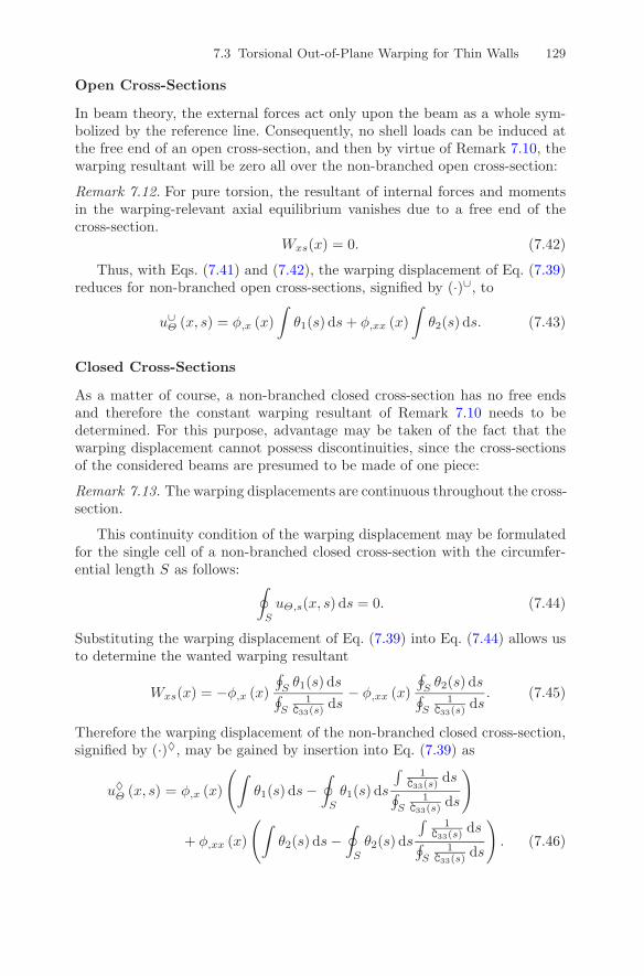
7.3 Torsional Out-of-Plane Warping for Thin Walls 129
Open Cross-Sections
In beam theory, the external forces act only upon the beam as a whole sym-bolized by the reference line. Consequently, no shell loads can be induced atthe free end of an open cross-section, and then by virtue of Remark 7.10, thewarping resultant will be zero all over the non-branched open cross-section:
Remark 7.12. For pure torsion, the resultant of internal forces and momentsin the warping-relevant axial equilibrium vanishes due to a free end of thecross-section.
Wxs(x) = 0. (7.42)
Thus, with Eqs. (7.41) and (7.42), the warping displacement of Eq. (7.39)reduces for non-branched open cross-sections, signified by (·)∪, to
u∪Θ (x, s) = φ,x (x)
∫
θ1(s) ds+ φ,xx (x)∫
θ2(s) ds. (7.43)
Closed Cross-Sections
As a matter of course, a non-branched closed cross-section has no free endsand therefore the constant warping resultant of Remark 7.10 needs to bedetermined. For this purpose, advantage may be taken of the fact that thewarping displacement cannot possess discontinuities, since the cross-sectionsof the considered beams are presumed to be made of one piece:
Remark 7.13. The warping displacements are continuous throughout the cross-section.
This continuity condition of the warping displacement may be formulatedfor the single cell of a non-branched closed cross-section with the circumfer-ential length S as follows:
∮
S
uΘ,s(x, s) ds = 0. (7.44)
Substituting the warping displacement of Eq. (7.39) into Eq. (7.44) allows usto determine the wanted warping resultant
Wxs(x) = −φ,x (x)
∮
Sθ1(s) ds
∮
S1
C33(s)ds
− φ,xx (x)
∮
Sθ2(s) ds
∮
S1
C33(s)ds
. (7.45)
Therefore the warping displacement of the non-branched closed cross-section,signified by (·)♦, may be gained by insertion into Eq. (7.39) as
u♦Θ (x, s) = φ,x (x)
(∫
θ1(s) ds −∮
S
θ1(s) ds
∫1
C33(s)ds
∮
S1
C33(s)ds
)
+ φ,xx (x)
(∫
θ2(s) ds −∮
S
θ2(s) ds
∫1
C33(s)ds
∮
S1
C33(s)ds
)
. (7.46)

130 7 Adaptive Thin-Walled Beams
7.3.3 General Cross-Sections with Open Branches and ClosedCells
A general cross-section consists of the branches i, joined at the junctionsj, and possibly forming the closed cells k. For every branch i, the warpingfunction uΘ i(x, s) may be derived from Eq. (7.39) with the warping resultantWxs i(x) and the integration constant Ci(x), since continuity of the curvilinearcoordinate s is ensured only within the branches:
∀i : uΘ i (x, s) = φ,x (x)∫
θ1(s) ds+ φ,xx (x)∫
θ2(s) ds
+Wxs i(x)∫
1C33 (s)
ds+ Ci (x) . (7.47)
As the curvilinear coordinate s may be defined separately for every branch,the associated directions are possibly dissimilar at junctions and around cells,see the example of Figure 7.2. To account for these dissimilar directions in thesubsequent examinations, the following association functions is introduced:
f ij =
{1 if i → j,
−1 if i ← j,f i
k =
{1 if i⇒ k,
−1 if i� k.(7.48)
The function f ij introduces a negative sign when the curvilinear coordinate
s in the branch i is not pointing towards the junction j. Correspondingly,the function f i
k introduces a negative sign when the curvilinear coordinate sin the branch i does not coincide with the common sense of direction in thecell k.
Fig. 7.2. Description of an exemplary cross-section with two adjoined cells k, formedby two junctions j and three branches i. With the optional slit at the dashed line,it may be converted into a combined cross-section consisting of a single closed celland two branches with free ends.
Open Branches
Here those branches will be considered that do not participate in the formationof a closed cell. They possess one free end, and the same reasoning as in the

7.3 Torsional Out-of-Plane Warping for Thin Walls 131
case of the non-branched open cross-section may be applied. Hence, for everyopen branch i not belonging to any of the closed cells k, the warping resultantWxs i(x) vanishes by virtue of Remark 7.12:
∀i /∈ k :Wxs i(x) = 0. (7.49)
Closed Cells
Also, just as in the case of the non-branched closed cross-section, the warpingresultant Wxs i(x) does not vanish in a closed cell. In accordance with Re-mark 7.13, the continuity of warping displacements around such a cell may berequired. The integration around closed cells must be performed in the samedirection over the participating branches, see also Gjelsvik [85]. With the aidof the association function f i
k, the continuity requirement may be formulatedfor every closed cell k with the circumferential length Sk assembled from thelengths Si of the participating branches i as follows:
∀k :∮
Sk
uΘ,s(x, s) ds =∑
i∈k
f ik
∫
Si
uΘ i,s(x, s) ds = 0. (7.50)
The connection of closed cells through the sharing of a common branch rep-resents a statically indeterminate system. Due to the excess of branches withregard to cells and junctions respectively, the unknown warping resultantsmay only be determined by both continuity requirements of the cells andaxial equilibrium conditions at the junctions.
Junctions
Such equilibrium conditions are only relevant for the case of multiple adjoinedcells, since the warping resultants of open branches and separate cells areeffectively determined by Eq. (7.49), respectively by Eq. (7.50). The axialequilibrium at the junctions j requires the consideration of the coordinatedirection in the cross-sectional plane of every involved branch i captured bythe association function f i
j . Thus, the following may be formulated:
∀j :∑
i∈j
f ijWxs i(x) = 0. (7.51)
Further on, the continuity requirement, as imposed by Remark 7.13, alsoapplies to the warping displacements of all branches meeting at a junction,which thus have to be identical there. Since an arrangement like Eq. (7.41) canbe made only for one branch, the integration constants Ci(x) of the remainingbranches may be determined.
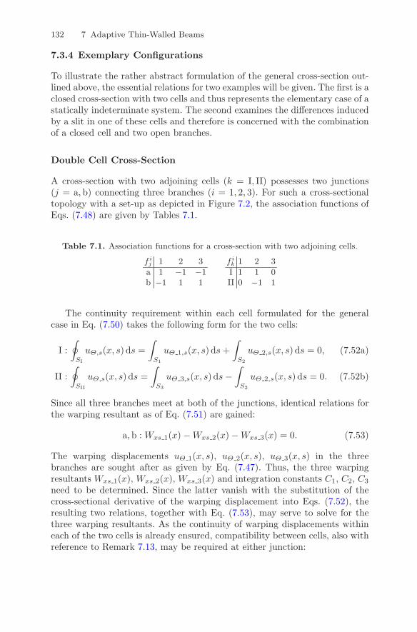
132 7 Adaptive Thin-Walled Beams
7.3.4 Exemplary Configurations
To illustrate the rather abstract formulation of the general cross-section out-lined above, the essential relations for two examples will be given. The first is aclosed cross-section with two cells and thus represents the elementary case of astatically indeterminate system. The second examines the differences inducedby a slit in one of these cells and therefore is concerned with the combinationof a closed cell and two open branches.
Double Cell Cross-Section
A cross-section with two adjoining cells (k = I, II) possesses two junctions(j = a, b) connecting three branches (i = 1, 2, 3). For such a cross-sectionaltopology with a set-up as depicted in Figure 7.2, the association functions ofEqs. (7.48) are given by Tables 7.1.
Table 7.1. Association functions for a cross-section with two adjoining cells.
f ij 1 2 3
a 1 −1 −1b −1 1 1
f ik 1 2 3
I 1 1 0II 0 −1 1
The continuity requirement within each cell formulated for the generalcase in Eq. (7.50) takes the following form for the two cells:
I :∮
SI
uΘ,s(x, s) ds =∫
S1
uΘ 1,s(x, s) ds+∫
S2
uΘ 2,s(x, s) ds = 0, (7.52a)
II :∮
SII
uΘ,s(x, s) ds =∫
S3
uΘ 3,s(x, s) ds −∫
S2
uΘ 2,s(x, s) ds = 0. (7.52b)
Since all three branches meet at both of the junctions, identical relations forthe warping resultant as of Eq. (7.51) are gained:
a, b :Wxs 1(x) − Wxs 2(x) − Wxs 3(x) = 0. (7.53)
The warping displacements uΘ 1(x, s), uΘ 2(x, s), uΘ 3(x, s) in the threebranches are sought after as given by Eq. (7.47). Thus, the three warpingresultants Wxs 1(x), Wxs 2(x), Wxs 3(x) and integration constants C1, C2, C3
need to be determined. Since the latter vanish with the substitution of thecross-sectional derivative of the warping displacement into Eqs. (7.52), theresulting two relations, together with Eq. (7.53), may serve to solve for thethree warping resultants. As the continuity of warping displacements withineach of the two cells is already ensured, compatibility between cells, also withreference to Remark 7.13, may be required at either junction:

7.3 Torsional Out-of-Plane Warping for Thin Walls 133
a : uΘ 1(x, S1) = uΘ 2(x, 0) = uΘ 3(x, 0), (7.54a)
b : uΘ 1(x, 0) = uΘ 2(x, S2) = uΘ 3(x, S3). (7.54b)
Besides the utilization of two independent relations out of these four rela-tions, additional information is necessary to determine the three integrationconstants. Here the zero passage of the warping displacement in the mannerof Eq. (7.41) may be introduced for one of the branches. For the example athand, this could be given for the center of the web as follows:
uΘ 2
(
x,S2
2
)
= 0.
So, the integration constants can be found and the warping displacementcompleted. However, since the formulation is rather lengthy, it will be omittedhere and, instead, only the result is shown in Figure 7.3.
Fig. 7.3. Warping displacement of a cross-section with two closed cells and allthrough identical constitutive properties.
Combined Cross-Section
When one of the cells of the previous configuration is slit, for example, at thedashed line in Figure 7.2, then four branches (i = 1, 2, 3a, 3b) and still twojunctions (j = a, b) need to be considered. The remaining closed cell (k = I)is formed by the two branches (i = 1, 2), while the other two (i = 3a, 3b)have free ends. As required by Eq. (7.49), the warping resultants of the lattertherefore have to vanish:
Wxs 3a(x) = 0, Wxs 3b(x) = 0. (7.55)
Consequently, they do not influence the axial equilibrium at the junctionsand, hence, Eq. (7.53) reduces to
a, b :Wxs 1(x) − Wxs 2(x) = 0. (7.56)
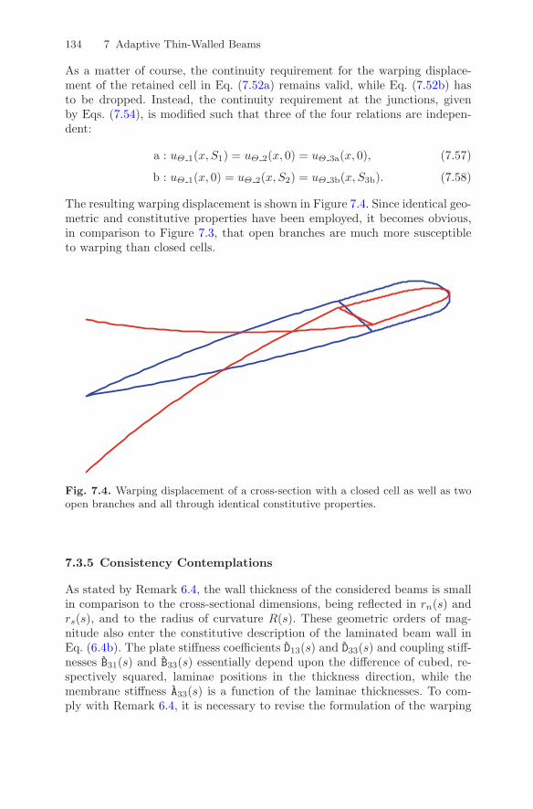
134 7 Adaptive Thin-Walled Beams
As a matter of course, the continuity requirement for the warping displace-ment of the retained cell in Eq. (7.52a) remains valid, while Eq. (7.52b) hasto be dropped. Instead, the continuity requirement at the junctions, givenby Eqs. (7.54), is modified such that three of the four relations are indepen-dent:
a : uΘ 1(x, S1) = uΘ 2(x, 0) = uΘ 3a(x, 0), (7.57)
b : uΘ 1(x, 0) = uΘ 2(x, S2) = uΘ 3b(x, S3b). (7.58)
The resulting warping displacement is shown in Figure 7.4. Since identical geo-metric and constitutive properties have been employed, it becomes obvious,in comparison to Figure 7.3, that open branches are much more susceptibleto warping than closed cells.
Fig. 7.4. Warping displacement of a cross-section with a closed cell as well as twoopen branches and all through identical constitutive properties.
7.3.5 Consistency Contemplations
As stated by Remark 6.4, the wall thickness of the considered beams is smallin comparison to the cross-sectional dimensions, being reflected in rn(s) andrs(s), and to the radius of curvature R(s). These geometric orders of mag-nitude also enter the constitutive description of the laminated beam wall inEq. (6.4b). The plate stiffness coefficients D13(s) and D33(s) and coupling stiff-nesses B31(s) and B33(s) essentially depend upon the difference of cubed, re-spectively squared, laminae positions in the thickness direction, while themembrane stiffness A33(s) is a function of the laminae thicknesses. To com-ply with Remark 6.4, it is necessary to revise the formulation of the warping

7.3 Torsional Out-of-Plane Warping for Thin Walls 135
displacement with its integrands given by Eqs. (7.40a) and (7.40b). Allow-ing for different degrees of approximation, a thorough treatment shows thedomination of the membrane response:
θ1 (s) ≈ rn (s) , θ2 (s) ≈ 0, and C33 (s) ≈ A33 (s) . (7.59)
Also in consideration of the rather small influence of the warping effect ingeneral, it seems reasonable to refrain from higher order warping influencesassociated with the second derivative of twist φ,xx(x).
Remark 7.14. For the approximation of the torsional out-of-plane warping dis-placement, only the dependence upon the rate of twist will be considered.
Thus, the description of the warping displacement breaks up into a com-ponent with axial dependence, the rate of twist φ,x(x), and one with cross-sectional dependence, the warping function Θ(s), like that being used in Sec-tion 7.2:
uΘ (x, s) = Θ (s)φ,x (x) . (7.60)
Resulting Simplifications
The implications of the approximation introduced by Eqs. (7.59) will bedemonstrated by means of the warping functions for the non-branched cross-sections. In the case of an open topology, as described by Eq. (7.43), eventhough the wall properties are anisotropic and may vary along the cross-sectional coordinate, the result is a purely geometric warping function
Θ∪ (s) =∫
rn(s) ds. (7.61)
In consideration of Eq. (7.27), this simplification leads in Eq. (7.31) to thedecoupling of the shear strain γ0
xs(x, s) from the twist rate φ,x(x). This is notgiven in the case of closed cross-sections, since an additional term is containedin the warping function
Θ♦ (s) =∫
rn(s) ds − 2A0
∫1
A33(s)ds
∮
S1
A33(s)ds
. (7.62)
When the constitutive properties of the wall are constant all around the cell,their influence vanishes and a purely geometric warping function remains,identical to the one determined via the shear flow of Bredt [24] for the isotropiccase:
Θ♦ (s) =∫
rn(s) ds − 2A0s
S. (7.63)
In Eqs. (7.62) and (7.63), the area enclosed by the wall of the single cell canbe identified and abbreviated by A0. Analogously, such an abridgment may

136 7 Adaptive Thin-Walled Beams
be introduced for cross-sections with multiple cells with the area Ak enclosedby cell k:
∮
S
rn(s) ds = 2A0, (7.64a)
∀k :∮
Sk
rn(s) ds =∑
i∈k
f ik
∫
Si
rn(s) ds = 2Ak. (7.64b)
7.4 Rotating Beams
So far, the beam itself has been described in detail. Now, it will be consideredas part of a rotating system. To herald the examination of inertia effects, it isnecessary to link the above kinematic relations to the description of a guidedmotion.
7.4.1 Rotor Kinematics
With regard to a guided motion around a fixed axis of rotation, it is essentialto refer to three different frames of reference. First, the inertial reference framedefines the global origin. Second, the rotating reference frame implements therotation around the origin. And third, the moving reference frame is associatedwith the mounting point of the beam. There the beam will be attached withthe following implications:
Remark 7.15. Clamped boundary conditions apply at the origin of the beam’scoordinate.
Thus, the considered moving reference frame agrees with the coordinatesystem introduced to describe the beam. Therein the position of an arbitrarypoint is represented by the vector po(x, s, t) according to Eq. (7.2) with themodified cross-sectional description for thin-walled beams of Eq. (7.16) inview of Eq. (7.1) and depending on time to accommodate dynamic beamdeformations. This position may be expressed in the inertial reference frameby the vector
p(x, s, t) = TΩ (t) (r + T321 (t) po(x, s, t)) . (7.65)
The position of the moving reference frame with respect to the rotating ref-erence frame is given by the vector r, while its orientation is specified by therotational transformation T321(t). This may be assembled from the rotationsaround individual axes:

7.4 Rotating Beams 137
T321 (t) = T3 (t)T2 (t)T1 (t)
with T3 (t) =
⎡
⎣cos(α3 (t)) − sin(α3 (t)) 0sin(α3 (t)) cos(α3 (t)) 0
0 0 1
⎤
⎦ ,
T2 (t) =
⎡
⎣cos(α2 (t)) 0 sin(α2 (t))
0 1 0− sin(α2 (t)) 0 cos(α2 (t))
⎤
⎦ ,
T1 (t) =
⎡
⎣1 0 00 cos(α1 (t)) − sin(α1 (t))0 sin(α1 (t)) cos(α1 (t))
⎤
⎦ .
(7.66)
Since the Cardan angles α3(t), α2(t), and α1(t) are prescribed parameters, adiscussion on the uniqueness of representation in analogy to Section 7.1.2 isnot necessary and we may simply agree upon their sequence. The orientation ofthe rotating reference frame relative to the inertial reference frame is describedby the rotational transformation
TΩ (t) =
⎡
⎣cos(αΩ (t)) − sin(αΩ (t)) 0sin(αΩ (t)) cos(αΩ (t)) 0
0 0 1
⎤
⎦ . (7.67)
For the sake of simplicity, the orientation of the inertial reference frame maybe chosen such that one of its axes represents the axis of rotation. In the caseof Eq. (7.67), the rotation occurs around the third axis of the inertial referenceframe.
7.4.2 Transformation Properties
The angle αΩ(t) may be expressed in terms of the angular velocity Ω(t) asfollows:
αΩ (t) =∫
Ω (t) dt. (7.68)
Then the derivatives in time of the rotational transformation TΩ (t), as givenby Eq. (7.67), are of the following form:
TΩ,t (t) = Ω (t)T′Ω (t) , TΩ,tt (t) = Ω,t (t)T′
Ω (t) +Ω2 (t)T′ ′Ω (t) . (7.69)
The matrices T′Ω(t) and T′ ′
Ω(t) contained therein represent the external deriv-atives and consequently read
T′Ω (t) =
⎡
⎣− sin(αΩ (t)) − cos(αΩ (t)) 0cos(αΩ (t)) − sin(αΩ (t)) 0
0 0 0
⎤
⎦ , (7.70a)
T′ ′Ω (t) =
⎡
⎣cos(αΩ (t)) − sin(αΩ (t)) 0sin(αΩ (t)) cos(αΩ (t)) 0
0 0 0
⎤
⎦ . (7.70b)

138 7 Adaptive Thin-Walled Beams
In the subsequent derivation, products of the matrix transpose of the transfor-mation TΩ(t) with itself or its derivatives will appear. The decisive propertyof these products is a separation of the time-dependent components from thematrix structure, such that the angular velocity Ω(t) and its derivative turnup only as scalar factors:
TTΩ (t)TΩ (t) = I, (7.71a)
TTΩ (t)TΩ,t (t) = Ω (t) I′, (7.71b)
TTΩ (t)TΩ,tt (t) = Ω,t (t) I′ +Ω2 (t) I′ ′. (7.71c)
The matrices I, I′, and I′ ′ are the identity matrix, and are filled with anantimetric submatrix and a negated identity submatrix, respectively:
I =
⎡
⎣1 0 00 1 00 0 1
⎤
⎦ , I′ =
⎡
⎣0 −1 01 0 00 0 0
⎤
⎦ , I′ ′ =
⎡
⎣−1 0 00 −1 00 0 0
⎤
⎦ . (7.72)
Analogous considerations also hold for the other above-mentioned transforma-tions of Eq. (7.66). However, when products of such matrices with incorpo-rated time dependence are nested, complications arise as soon as the centralproduct contains a derivative. Thus, time-dependent matrices do not occur, forexample, in the product TT
1 (t)TTΩ(t)TΩ(t)T1(t), which still yields the identity
matrix, but cannot be avoided for the likes of TT1 (t)TT
Ω(t)TΩ,t(t)T1(t).
8
Virtual Work Statements
To determine the equations of equilibrium as well as the constitutive relationsof the beam, the principle of virtual work may be applied and its individualcontributions be examined, respectively. Thus, the foundations for an ana-lytic solution with regard to the statics of the non-rotating structure can beprovided. Furthermore, the principle of virtual work will serve to set up theequations of motion in consideration of the dynamics of the rotating struc-ture. This, in addition, requires the study of inertia effects and the inclusionof stiffening effects due to kinematic non-linearity with reference to relativelyslender and flexible beams. The derivation of the principle of virtual work forthe general case is presented in Section 3.4, and it will now be adapted andextended to depict adaptive thin-walled beams. Therefore, the various virtualwork contributions will be discussed individually.
8.1 Internal Virtual Work
The virtual work of internal contributions is assembled in Section 3.4.6 fromthe virtual strain energy and virtual work of internal charges, as suppliedby the principle of virtual displacements and of virtual electric potential,respectively. In Eq. (3.63), the virtual work of internal contributions is givenfor a volumetric object. The preceding analysis accomplished a reduction totwo dimensions for the shell-like wall and to one dimension for the beam.Consequently, the expression for the virtual work of internal contributionsmay be reformulated for the wall δU (t) and for the beam δU (t) as follows:
δU (t) =∫
X
δχT (x) L (x, t) dx, (8.1a)
�
δU (t) =∫
X
∫
S
δχT (x, s) L (x, s, t) dsdx
=∫
X
δχT (x)∫
S
JT (s) L (x, s, t) dsdx. (8.1b)
T.H. Brockmann, Theory of Adaptive Fiber Composites,Solid Mechanics and Its Applications 161,c© Springer Science + Business Media B.V. 2009
140 8 Virtual Work Statements
In the lower line, use has been made of the relation between strain and electricfield strength measures of wall and beam, provided by Eq. (7.33) and adaptedto the virtual expressions.
8.1.1 Internal Loads of Beam and Wall
As a matter of course, the virtual work needs to be independent of the descrip-tion. Thus, equating Eqs. (8.1) allows us to associate the internal mechanicalas well as electric loads of beam L(x, t) and wall L(x, s, t):
δU (t) = δU (t) → L (x, t) =∫
S
JT (s) L (x, s, t) ds. (8.2)
Obtaining the entries of the matrix J(s) of Eq. (7.33) from Eqs. (7.31) and(7.32) leads, with the internal loads L(x, s, t) of the wall as listed in Eq. (6.6),to
L (x, t)=
⎧⎪⎪⎪⎪⎪⎪⎪⎪⎪⎪⎪⎪⎪⎪⎪⎪⎪⎪⎪⎪⎪⎨
⎪⎪⎪⎪⎪⎪⎪⎪⎪⎪⎪⎪⎪⎪⎪⎪⎪⎪⎪⎪⎪⎩
N(x, t)Qy(x, t)Qz(x, t)Mx(x, t)My(x, t)Mz(x, t)Qw(x, t)
−Gc (x, t)Gd (x, t)
...
⎫⎪⎪⎪⎪⎪⎪⎪⎪⎪⎪⎪⎪⎪⎪⎪⎪⎪⎪⎪⎪⎪⎬
⎪⎪⎪⎪⎪⎪⎪⎪⎪⎪⎪⎪⎪⎪⎪⎪⎪⎪⎪⎪⎪⎭
=
⎧⎪⎪⎪⎪⎪⎪⎪⎪⎪⎪⎪⎪⎪⎪⎪⎪⎪⎪⎪⎪⎪⎪⎪⎨
⎪⎪⎪⎪⎪⎪⎪⎪⎪⎪⎪⎪⎪⎪⎪⎪⎪⎪⎪⎪⎪⎪⎪⎩
∫
SNx (x, s, t) ds
∫
Sy,s (s)Nxs (x, s, t) + 1
2z,ss (s)Mxs (x, s, t) ds∫
Sz,s (s)Nxs (x, s, t) − 1
2y,ss (s)Mxs (x, s, t) ds∫
SΦ (s)Nxs (x, s, t) − (2 + 1
2Φ(s)R(s) )Mxs (x, s, t) ds
∫
Sz (s)Nx (x, s, t) + y,s (s)Mxx (x, s, t) ds
∫
S−y (s)Nx (x, s, t) + z,s (s)Mxx (x, s, t) ds
∫
SΘ (s)Nx (x, s, t) − rs (s)Mxx (x, s, t) ds
−∫
Spc (s)Gc
3 (x, s, t) ds∫
Spd (s)Gd
3 (x, s, t) ds...
⎫⎪⎪⎪⎪⎪⎪⎪⎪⎪⎪⎪⎪⎪⎪⎪⎪⎪⎪⎪⎪⎪⎪⎪⎬
⎪⎪⎪⎪⎪⎪⎪⎪⎪⎪⎪⎪⎪⎪⎪⎪⎪⎪⎪⎪⎪⎪⎪⎭
.
(8.3)
8.1.2 Constitutive Relation
The constitutive relation of an adaptive laminated composite shell is given inEq. (6.6). Being considered for the thin wall of the beam, the lines, respectivelycolumns, associated with the cross-sectional strain component ε0s(x, s) andbending curvature κs(x, s) can be dropped in accordance with Remark 7.4.To comply with the specification of a prismatic beam in Remark 7.1, alsowith regard to the material properties, the latter need to be constant alongthe lengthwise direction and thus the constitutive matrix K(s) only dependson the cross-sectional coordinate. The constitutive relation of the wall and thecorresponding formulation for the beam with the constitutive matrix P then

8.1 Internal Virtual Work 141
read:L (x, s, t) = K (s) χ (x, s, t) , L (x, t) = Pχ (x, t) . (8.4)
Insertion of these constitutive relations into the virtual work of internal loadsof the wall δU (t) and of the beam δU (t) as expressed by Eqs. (8.1) results in
δU (t) =∫
X
δχT (x) Pχ (x, t) dx, (8.5a)
�
δU (t) =∫
X
∫
S
δχT (x, s) K (s) χ (x, s, t) dsdx
=∫
X
δχT (x)∫
S
JT (s) K (s) J (s) dsχ (x, t) dx. (8.5b)
For the lower line, use has been made again of the relation between strainand electric field strength measures of wall and beam provided by Eq. (7.33).Similarly, the constitutive matrix of the beam may be identified:
δU (t) = δU (t) → P =∫
S
JT (s) K (s) J (s) ds. (8.6)
8.1.3 Constitutive Coefficients
For the considered beams of arbitrary cross-sections with anisotropic wallsand adaptive capabilities, a multitude of mechanical and electromechanicalcoupling mechanisms arise. They are reflected in the off-diagonal entries ofthe beam constitutive matrix P. As defined in Eq. (8.6), the latter containsthe geometry and warping functions responsible for couplings that may beattributed to the cross-sectional level, as well as the constitutive coefficientsof the shell. These entries of the matrix K(s) may be again assigned to twodifferent coupling levels. Coupling on the laminae level is founded on theexistence of associated off-diagonal entries in the property matrix Q of theindividual laminae, see Eq. (4.31). It may also appear in the case of sym-metric laminates. Coupling on the laminate level, in contrast stems from anon-symmetric set-up of the laminate. For the case at hand, the shell stiffnesscoefficients A13(s), B13(s), B31(s), and D13(s) represent the mechanical couplingon the laminae level, while the coefficients B11(s), B13(s), B31(s), B33(s) char-acterize the mechanical coupling on the laminate level. Since the coefficientsB13(s) and B31(s) are associated with both levels, they only exist when bothrequirements are fulfilled. Analogously, also the electromechanical coefficientscan be associated with the constitutive coupling levels. Such a classificationmay be used to examine the consequences of simplifying assumptions on thedifferent levels.
142 8 Virtual Work Statements
Mechanical Coefficients on the Principal Diagonal
The beam stiffness coefficients on the principal diagonal of the matrix P as-sociated with extension, P11, bending, P55, P66, and warping, P77, depend onthe shell stiffnesses associated with the lengthwise extension, A11(s), bending,D11(s), and the coupling B11(s):
P11 =∫
S
A11 (s) ds, (8.7a)
P55 =∫
S
A11 (s) z2 (s) + 2B11 (s) z (s) y,s (s) + D11 (s) y2,s (s) ds, (8.7b)
P66 =∫
S
A11 (s) y2 (s) − 2B11 (s) y (s) z,s (s) + D11 (s) z2,s (s) ds, (8.7c)
P77 =∫
S
A11 (s)Θ2 (s) − 2B11 (s)Θ (s) rs (s) + D11 (s) r2s (s) ds. (8.7d)
The other beam stiffness coefficients on the principal diagonal associated withshear, P22, P33, and torsion, P44, are functions of the shell stiffnesses associatedwith shear, A33(s), twist, D33(s), and the coupling B33(s):
P22 =∫
S
A33 (s) y2,s (s) + B33 (s) y,s (s) z,ss (s) + D33 (s)z2,ss (s)
4ds, (8.8a)
P33 =∫
S
A33 (s) z2,s (s) − B33 (s) z,s (s) y,ss (s) + D33 (s)y2,ss (s)
4ds, (8.8b)
P44 =∫
S
A33 (s)Φ2 (s) − 2B33 (s)Φ (s)(
2 +Φ (s)2R (s)
)
+ D33 (s)(
2 +Φ (s)2R (s)
)2
ds. (8.8c)
Off-Diagonal Mechanical Coefficients without Laminae LevelCoupling
Likewise, the beam stiffness coefficients which couple extension, bending inboth directions, and warping depend on the shell stiffnesses associated withthe lengthwise extension, bending, and coupling between them:
P15 =∫
S
A11 (s) z (s) + B11 (s) y,s (s) ds, (8.9a)
P16 =∫
S
−A11 (s) y (s) + B11 (s) z,s (s) ds, (8.9b)
P17 =∫
S
A11 (s)Θ (s) − B11 (s) rs (s) ds, (8.9c)

8.1 Internal Virtual Work 143
P56 =∫
S
−A11 (s) y (s) z (s) − B11 (s) (y (s) y,s (s) − z (s) z,s (s))
+ D11 (s) y,s (s) z,s (s) ds, (8.9d)
P57 =∫
S
A11 (s)Θ (s) z (s) + B11 (s) (Θ (s) y,s (s) − rs (s) z (s))
− D11 (s) rs (s) y,s (s) ds, (8.9e)
P67 =∫
S
−A11 (s)Θ (s) y (s) + B11 (s) (Θ (s) z,s (s) + rs (s) y (s))
− D11 (s) rs (s) z,s (s) ds. (8.9f)
The beam stiffness coefficients, which couple shear in both directions andtorsion, are functions of the shell stiffnesses associated with shear, twist, andthe coupling between them:
P23 =∫
S
A33 (s) y,s (s) z,s (s) +B33 (s)
2(z,s (s) z,ss (s) − y,s (s) y,ss (s))
− D33 (s)y,ss (s) z,ss (s)
4ds, (8.10a)
P24 =∫
S
A33 (s)Φ (s) y,s (s) + B33 (s)(
Φ (s)z,ss (s)
2−(
2 +Φ (s)2R (s)
)
y,s (s))
− D33 (s)(
2 +Φ (s)2R (s)
)z,ss (s)
2ds, (8.10b)
P34 =∫
S
A33 (s)Φ (s) z,s (s) − B33 (s)(
Φ (s)y,ss (s)
2+(
2 +Φ (s)2R (s)
)
z,s (s))
+ D33 (s)(
2 +Φ (s)2R (s)
)y,ss (s)
2ds. (8.10c)
Off-Diagonal Mechanical Coefficients with Laminae Level Coupling
The remaining beam stiffness coefficients depend on the shell stiffnesses thatresult from coupling on the laminae level. This concerns the coupling be-tween shear and extension, A13(s), between extension and lengthwise curva-ture, B13(s) and B31(s), as well as between lengthwise curvature and twist,D13(s). So, the beam stiffness coefficients responsible for the coupling of ex-tension with shear and torsion read:

144 8 Virtual Work Statements
P12 =∫
S
A13 (s) y,s (s) +B13 (s)
2z,ss (s) ds, (8.11a)
P13 =∫
S
A13 (s) z,s (s) − B13 (s)2
y,ss (s) ds, (8.11b)
P14 =∫
S
A13 (s)Φ (s) − B13 (s)(
2 +Φ (s)2R (s)
)
ds. (8.11c)
The beam stiffness coefficients in charge of the coupling between shear andbending have the subsequent form:
P25 =∫
S
A13 (s) z (s) y,s (s) + B13 (s) z (s)z,ss (s)
2+ B31 (s) y2,s (s)
+ D13 (s) y,s (s)z,ss (s)
2ds, (8.12a)
P36 =∫
S
−A13 (s) y (s) z,s (s) + B13 (s) y (s)y,ss (s)
2+ B31 (s) z2,s (s)
− D13 (s) z,s (s)y,ss (s)
2ds, (8.12b)
P26 =∫
S
−A13 (s) y (s) y,s (s) − B13 (s) y (s)z,ss (s)
2+ B31 (s) y,s (s) z,s (s)
+ D13 (s) z,s (s)z,ss (s)
2ds, (8.12c)
P35 =∫
S
A13 (s) z (s) z,s (s) − B13 (s) z (s)y,ss (s)
2+ B31 (s) y,s (s) z,s (s)
− D13 (s) y,s (s)y,ss (s)
2ds. (8.12d)
The beam stiffness coefficients accounting for the coupling of bending andtwist are given as follows:
P45 =∫
S
A13 (s)Φ (s) z (s) − B13 (s)((
2 +Φ (s)2R (s)
)
z (s) − Φ (s) y,s (s))
− D13 (s)(
2 +Φ (s)2R (s)
)
y,s (s) ds, (8.13a)
P46 =∫
S
−A13 (s)Φ (s) y (s) + B13 (s)((
2 +Φ (s)2R (s)
)
y (s) + Φ (s) z,s (s))
− D13 (s)(
2 +Φ (s)2R (s)
)
z,s (s) ds. (8.13b)
Finally, the beam stiffness coefficients associated with the coupling of shearand torsion with warping read:

8.1 Internal Virtual Work 145
P27 =∫
S
A13 (s)Θ (s) y,s (s) + B13 (s)Θ (s)z,ss (s)
2− B31 (s) rs (s) y,s (s)
− D13 (s) rs (s)z,ss (s)
2ds, (8.14a)
P37 =∫
S
A13 (s)Θ (s) z,s (s) − B13 (s)Θ (s)y,ss (s)
2− B31 (s) rs (s) z,s (s)
+ D13 (s) rs (s)y,ss (s)
2ds, (8.14b)
P47 =∫
S
A13 (s)Φ (s)Θ (s) − B13 (s)(
2 +Φ (s)2R (s)
)
Θ (s) − B31 (s)Φ (s) rs (s)
+ D13 (s)(
2 +Φ (s)2R (s)
)
rs (s) ds. (8.14c)
Electromechanical Coefficients
Corresponding to the mechanical coefficients, those representing the electro-mechanical coupling due to the piezoelectric effect also may be arranged. Theinduction and detection of extension, bending, and warping of the beam de-pends on the electromechanical shell coefficients associated with extension,Ac14(s), and lengthwise curvature, Bc
14(s):
P18 =∫
S
Ac14 (s) pc (s) ds, (8.15a)
P58 =∫
S
(Ac14 (s) z (s) + Bc
14 (s) y,s (s)) pc (s) ds, (8.15b)
P68 =∫
S
(−Ac14 (s) y (s) + Bc
14 (s) z,s (s)) pc (s) ds, (8.15c)
P78 =∫
S
(Ac14 (s)Θ (s) − Bc
14 (s) rs (s)) pc (s) ds. (8.15d)
The induction and detection of shear and torsion of the beam is governed bythose electromechanical shell coefficients associated with shear, Ac
34(s), andtwist, Bc
34(s):
P28 =∫
S
(
Ac34 (s) y,s (s) + Bc
34 (s)z,ss (s)
2
)
pc (s) ds, (8.16a)
P38 =∫
S
(
Ac34 (s) z,s (s) − Bc
34 (s)y,ss (s)
2
)
pc (s) ds, (8.16b)
P48 =∫
S
(
Ac34 (s)Φ (s) − Bc
34 (s)(
2 +Φ (s)2R (s)
))
pc (s) ds. (8.16c)
The dielectric permittivity properties, summarized for the shell in the coeffi-cient Ac
44(s), are considered for the beam by integration over the cross-section:

146 8 Virtual Work Statements
P88 =∫
S
Ac44 (s) (pc (s))2 ds =
∫
S
Ac44 (s) ds. (8.17)
For further groups of electrically paralleled laminae, the formulation is anal-ogous.
Open Cross-Section Peculiarity
A prominent property of a non-branched and branched open cross-sectionas well as of open branches within a combined cross-section will be markedhere. By virtue of Eqs. (7.42) and (7.59), a purely geometric warping func-tion is found in these cases, as exemplarily shown for the non-branched opencross-section in Eq. (7.61). Accordingly, the abbreviation Φ(s) introduced inEq. (7.27) vanishes:
Φ∪ (s) = 0. (8.18)
This has thorough consequences for all torsion-related entries of the beamconstitutive matrix P, since it eliminates the dependence on the membraneproperties stemming from the shell constitutive sub-matrix A(s). The torsionalstiffness P44 of Eq. (8.8c) is only governed by the twisting stiffness of the wall:
P∪44 =
∫
S
4D33 (s) ds. (8.19)
Since a diagonal entry of the constitutive matrix must not be zero, it is ex-plained why those thin-walled beam theories, which only account for the mem-brane response, are limited to closed cross-sections. The above argument cor-respondingly applies to contributions of open branches within a combinedcross-section.
8.1.4 Partially Prescribed Electric Potential
In Section 4.5, the different variants of actuation and sensing with regardto the type of electric power supply and electric measurement, respectively,are discussed. For actuation in conjunction with a voltage source and sens-ing via current measurement, the electric potential is identified to be a pre-scribed quantity. Consequently, the variation of the corresponding electricfield strength vanishes and the principle of virtual work therefore needs to bemodified. To provide a general description, the vector of electric field strengthE(x, t), containing the values for all groups of electrically paralleled laminae,may be split into two parts, E†(x, t) and E‡(x, t). Herein, the unknown fieldsare elucidated by ()† and the prescribed fields by ()‡. The virtual work ofinternal contributions, given by Eq. (8.5a), therefore can be rewritten as

8.2 External Virtual Work 147
δU (t) =∫
X
{
δεT (x) δET
† (x) δET
‡ (x)}
︸ ︷︷ ︸δχT (x)
⎡
⎢⎣
p p† p‡
pT† Ip† 0
pT‡ 0 Ip‡
⎤
⎥⎦
︸ ︷︷ ︸P
⎧⎨
⎩
ε (x, t)E† (x, t)E‡ (x, t)
⎫⎬
⎭
︸ ︷︷ ︸χ(x,t)
dx.
(8.20)The decomposition of the constitutive matrix P of the beam reveals its purelymechanical part p, its electromechanically coupled parts p† and p‡, and itsdielectric diagonal entries p† and p‡. As addressed above, the virtual electricfield strength of the prescribed fields vanishes and thus δE‡(x) = 0. Thesummary of vectors and matrices with regard to the remaining degrees offreedom of the beam, comes to
δμ (x) ={δε (x)δE† (x)
}
, P =[
p p†pT
† Ip†
]
, μ (x, t) ={
ε (x, t)E† (x, t)
}
.
(8.21)Thus, the virtual work of internal contributions may be written in terms offunctions of the mechanical and electric degrees of freedom in δU me(t) andelectric parameters in δU pe(t) such that
δU (t) =∫
X
δμT (x)Pμ (x, t) dx︸ ︷︷ ︸
δU me(t)
+∫
X
δεT (x)p‡E‡ (x, t) dx︸ ︷︷ ︸
δU pe(t)
. (8.22)
For obvious reasons, such a partition cannot be carried out before the consti-tutive relation is introduced. Nevertheless, the formulation with internal loadsgiven by Eq. (8.1a) reduces for the vector L†(x, t) of the mechanical loads andthose electric loads not associated with an electric parameter, to
δU (t) =∫
X
δμT (x) L† (x, t) dx. (8.23)
8.2 External Virtual Work
Since beam theory is concerned with the representation of structures withessentially one dimension of extent, the mechanical and electric loads appliedto volumes and areas in Eq. (3.62) need to be assigned to the beam referenceline. The virtual work δV me(t) of such loads will be defined subsequentlyand, furthermore, the virtual work δV dl(t) of inertia loads will be derivedfor rotating systems. So, the virtual work of external loads altogether for thebeam reads:
δV (t) = δV me (t) + δV dl (t) . (8.24)

148 8 Virtual Work Statements
8.2.1 Applied Load Contributions
The virtual work δV me(t) of applied mechanical and electric loads involvesthe virtual variant δν(x) of the degrees of freedom ν(x, t) of the beam andthe actual applied loads l(x, t), resulting in
δV me (t) =∫
X
δνT (x) l (x, t) dx. (8.25)
Therefore, only applied loads associated with a degree of freedom are consid-ered, while consequently those associated with a parameter are discarded, cor-responding to the nature of the employed electric circuits. The vector ν(x, t)is assembled from the mechanical degrees of freedom u(x, t), which appear inEq. (7.25), and from the electric degrees of freedom ϕ(x, t), such that
ν (x, t) ={
u (x, t)ϕ (x, t)
}
with ϕ (x, t) ={ϕc (x, t) ϕd (x, t) . . .
}T , (8.26)
u (x, t) ={u (x, t) v (x, t) w (x, t) φ (x, t) βy (x, t) βz (x, t) φ,x (x, t)
}T .
Applied mechanical loads n(x, t) and applied electric loads g(x, t) form thevector of actual applied loads l(x, t). With the designation of its componentsin analogy to the internal loads of Eq. (8.3), it reads
l (x, t) ={
n (x, t)g (x, t)
}
with g (x, t) ={gc (x, t) gd (x, t) . . .
}T , (8.27)
n (x, t) ={n(x, t) qy(x, t) qz(x, t) mx(x, t) my(x, t) mz(x, t) qw(x, t)
}T.
8.2.2 Inertia Load Contributions
D’Alembert’s principle in the Lagrangian version has been obtained in Sec-tion 3.4.5 in terms of virtual displacements and actual accelerations. Sinceit needs to be accounted for a superimposed guided motion, the positionp (x, s, t) in the inertial frame of reference, as described by Eq. (7.65), hasto be taken into consideration. With the density ρ(s, n) in accordance withRemark 7.1, the virtual work of inertia forces originating from Eq. (3.59) thenreads
δV dl (t) = −∫
Λ
δpT (x, s, t) p,tt(x, s, t)ρ (s, n) dV . (8.28)
Taking the variation of Eq. (7.65), the global virtual position vector δp(x, s, t)in the inertial reference frame may be obtained in terms of the local virtualposition vector δpo(x, s) in the moving reference frame:
δp (x, s, t) = TΩ (t)T321 (t) δpo(x, s). (8.29)

8.2 External Virtual Work 149
Correspondingly, the acceleration p,tt(x, s, t) as the second derivative of theglobal position can be gained from Eq. (7.65). When this is done in considera-tion of Eqs. (7.69) and (7.70) and the rotational properties of Eqs. (7.71) and(7.72) are introduced to the vector product in the integrand of Eq. (8.28), weobtain
δpT (x, s, t) p,tt(x, s, t)
= δpTo (x, s)TT
321 (t)(Ω,t (t) I′ +Ω2 (t) I′ ′) (r + T321 (t) po(x, s, t))
+ 2δpTo (x, s)TT
321 (t) (Ω (t) I′)(T321 (t) po,t(x, s, t) + T321,t (t) po(x, s, t)
)
+ δpTo (x, s)TT
321 (t)(T321 (t) po,tt(x, s, t) + 2T321,t (t) po,t(x, s, t) + T321,tt (t) po(x, s, t)
).
(8.30)
In view of the above discussion on the transformation properties, it needs tobe noted that Eq. (8.30) and thus the resulting equations of motion containtime-dependent matrices. The mathematical theory for such non-autonomoussystems has primarily been developed with regard to a periodic dependenceon time. The most prominent approaches to solve these systems are the meth-ods of Floquet [75] and of Hill [95]. For further details, see Prothmann [146],Gasch and Knothe [78], or Meirovitch [125]. To pave the way for an eventu-ally autonomous system with a less expensive theoretical framework, not toexceed the scope of the study at hand, we will abstain from a time-dependentorientation of the clamping of the beam.
Remark 8.1. The rotation around an axis of the inertial reference frame willbe the only guided motion of the considered system.
Thus, the rotational transformation at the clamped end of the beam isrestricted to a constant description of the orientation:
T321 (t) = T321 = T3T2T1 with α3 (t) = α3, α2 (t) = α2, α1 (t) = α1.(8.31)
To determine the virtual work of inertia forces in terms of the beam displace-ments, the latter are used to express the beam positions and the derivativesand variation thereof respectively, as governed by Eqs. (7.2) and (7.25):
po,t(x, s, t) = K (s) u,t (x, t) ,
po(x, s, t) = P o (x, s) + K (s) u (x, t) → po,tt(x, s, t) = K (s) u,tt (x, t) ,
δpo(x, s) = K (s) δu (x) .(8.32)
Then substitution of Eq. (8.30) into (8.28) leads, with simplifications due toEq. (8.31), to an expression with the following classification of inertia terms:

150 8 Virtual Work Statements
δV dl (t) = −∫
X
δuT (x) (
M′ ′u,tt (x, t) relative acc.—effects without rotation+ M′2Ω (t) u,t (x, t) Coriolis acc.—gyroscopic effects+ MΩ2 (t) u (x, t) centrifugal acc.—effects due to deformation+ m (x)Ω2 (t) centrifugal acc.—effects in initial state+ M′Ω,t (t) u (x, t) angular acc.—effects due to deformation+ m′ (x)Ω,t (t) angular acc.—effects in initial state) dx. (8.33)
The appearing matrices and vectors contain the integration over the cross-section and, as anticipated, do not vary with time:
M′ ′ =∫
S
KT (s)K (s)∫
N
ρ (s, n) dnds, (8.34a)
M′ =∫
S
KT (s)TT321I
′T321K (s)∫
N
ρ (s, n) dnds, (8.34b)
M =∫
S
KT (s)TT321I
′ ′T321K (s)∫
N
ρ (s, n) dnds, (8.34c)
m′ (x) =∫
S
KT (s)TT321I
′ (r + T321P o (x, s))∫
N
ρ (s, n) dnds, (8.34d)
m (x) =∫
S
KT (s)TT321I
′ ′ (r + T321P o (x, s))∫
N
ρ (s, n) dnds. (8.34e)
As already obvious from the classification of terms in Eq. (8.33), the inertiaproperties contained in the matrix M′ ′ are those of the non-rotating beam.Therefore, they are necessarily independent of its orientation, which is assuredby the transformation property of the sequence of time-independent matricessuch that TT
321T321 = I.
8.2.3 Equilibrium and Boundary Conditions
With the aid of the principle of virtual work, the equilibrium and bound-ary conditions can be obtained for the quasi-static case, where, in principle,loads may change over time but inertia effects are not considered. The con-tributions required for this purpose have been already obtained and will bejoined together in the following. The internal virtual work δU (t) is given byEq. (8.23), while the external virtual work δV (t) of Eq. (8.24) reduces forthe quasi-static case to those contributions δV me(t) due to the applied loadsspecified in Eq. (8.25). For the considered situation, the simplified principleof virtual work then reads:
δU (t) = δV (t) →∫
X
δμT (x) L† (x, t) dx =∫
X
δνT (x) l (x, t) . (8.35)

8.3 Second-Order Theory 151
As was done in Section 6.2.3 to obtain the equilibrium equations of the shell,integration by parts is applied to the principle of virtual work with the objec-tive of eliminating the appearing derivatives of the beam’s degrees of freedom.The geometric boundary conditions (first column) for a cantilever configura-tion are employed to warrant admissible displacement states. To satisfy theprinciple, the integrands collected for all virtual displacements have to vanish,giving the equilibrium equations (second column). The remaining terms yieldthe natural boundary conditions (third column) at the free end:
u (x = 0) = 0, n (x, t) + N,x (x, t) = 0, N (x = X) = 0,(8.36a)
v (x = 0) = 0, qy (x, t) + Qy,x (x, t) = 0, Qy (x = X) = 0,(8.36b)
w (x = 0) = 0, qz (x, t) + Qz,x (x, t) = 0, Qz (x = X) = 0,(8.36c)
βy (x = 0) = 0, my (x, t) − Qz (x, t) + My,x (x, t) = 0, My (x = X) = 0,(8.36d)
βz (x = 0) = 0, mz (x, t) + Qy (x, t) + Mz,x (x, t) = 0, Mz (x = X) = 0.(8.36e)
The coupling of warping and torsion is manifested in the equilibrium equa-tions, as they do not appear separately:
mx (x, t) + Mx,x (x, t) − qw,x (x, t) − Qw,xx (x, t) = 0, (8.37a)
φ (x = 0) = 0, Mx (x = X) − qw (x = X) − Qw,x (x = X) = 0, (8.37b)
φ,x (x = 0) = 0, Qw (x = X) = 0. (8.37c)
The above procedure also provides corresponding sets of equations for theelectric loads of every group of electrically paralleled laminae:
ϕc (x = 0) = 0, gc (x, t) + Gc,x (x, t) = 0, Gc (x = X) = 0, (8.38a)
ϕd (x = 0) = 0, gd (x, t) + Gd,x (x, t) = 0, Gd (x = X) = 0. (8.38b)
......
...
8.3 Second-Order Theory
First-order theories are bound to the equilibrium of the undeformed systemand therefore are basically suitable for small deformations. Second-order theo-ries consider the equilibrium of the slightly deformed system and are necessaryto investigate tensioned flexible structures as well as buckling phenomena.Since the behavior in this context is frequently dominated by the normalforce, it is commonly not accounted for the other initial internal loads, while

152 8 Virtual Work Statements
they will be included in the subsequent derivation. Non-linear theories do notsuffer from the implications of the different linearization procedures and areable to depict larger deformations as they occur, for example, in the post-buckling state. The capabilities of such elaborate theories have to be acquiredat the cost of analytic insight and computational efficiency. With referenceto Section 7.1, it would be possible to employ a geometrically exact descrip-tion without reducing to small rotations, as of Remark 7.2. Such theorieshave been developed and advanced, for instance, by Simo and Vu-Quoc [164],Hodges [97], and Gruttmann et al. [89] for beams without adaptive capabili-ties.
8.3.1 Additional Internal Load Contributions
The non-linear strain measures for the most general comprehensible case,involving finite displacements but small rotations of the beam, are derivedin Section 7.1 and given by Eq. (7.15). In accordance with the calculus ofvariations, see Funk [77], the virtual variant of these strain measures reads
δεGL (x) =
⎧⎪⎪⎪⎪⎪⎪⎪⎪⎨
⎪⎪⎪⎪⎪⎪⎪⎪⎩
δu,x (x)−δβz (x) + δv,x (x)δβy (x) + δw,x (x)
δφ,x (x)δβy,x (x)δβz,x (x)δφ,xx (x)
⎫⎪⎪⎪⎪⎪⎪⎪⎪⎬
⎪⎪⎪⎪⎪⎪⎪⎪⎭
︸ ︷︷ ︸δε(x)
+
⎧⎪⎪⎪⎪⎪⎪⎪⎪⎨
⎪⎪⎪⎪⎪⎪⎪⎪⎩
v,x (x) δv,x (x) + w,x (x) δw,x (x)φ (x) δw,x (x) + w,x (x) δφ (x)
−φ (x) δv,x (x) − v,x (x) δφ (x)0
−φ,x (x) δv,x (x) − v,x (x) δφ,x (x)−φ,x (x) δw,x (x) − w,x (x) δφ,x (x)
0
⎫⎪⎪⎪⎪⎪⎪⎪⎪⎬
⎪⎪⎪⎪⎪⎪⎪⎪⎭
︸ ︷︷ ︸δε(x)
.
(8.39)As shown here, the strains may be split into the linear part δε(x) and thenon-linear part δε(x). The prior corresponds to the variation of the linearstrain measures as they are obtained for the thin-walled beam in Section 7.2and given by Eq. (7.31). Further on, the internal loads vector N(x, t) of thebeam can be subdivided into the portion N(x, t), associated with the initialconfiguration, and the portion N(x, t) related to the superposed deformation.Then the virtual strain energy δU md(t), based on the general formulation ofEq. (3.45), may be written for the beam as follows:
δU md (t)
=∫
X
δεTGL (x) N (x, t) dx with N (x, t) = N (x, t) + N (x, t)
=∫
X
δεT (x) N (x, t) dx︸ ︷︷ ︸
δU md(t)
+∫
X
δεT (x) N (x, t) dx︸ ︷︷ ︸
δU ms(t)
+∫
X
δεT (x) N (x, t) dx︸ ︷︷ ︸
.
→ 0
(8.40)
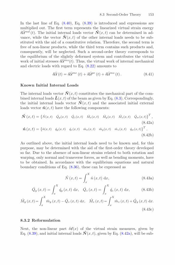
8.3 Second-Order Theory 153
In the last line of Eq. (8.40), Eq. (8.39) is introduced and expressions aremultiplied out. The first term represents the linearized virtual strain energyδU md (t). The initial internal loads vector N(x, t) can be determined in ad-vance, while the vector N(x, t) of the other internal loads needs to be sub-stituted with the aid of a constitutive relation. Therefore, the second term isfree of non-linear products, while the third term contains such products and,consequently, will be neglected. Such a second-order theory corresponds tothe equilibrium of the slightly deformed system and contributes the virtualwork of initial stresses δU ms(t). Thus, the virtual work of internal mechanicaland electric loads with regard to Eq. (8.22) amounts to
δU (t) = δU me (t) + δU pe (t) + δU ms (t) . (8.41)
Known Initial Internal Loads
The internal loads vector N(x, t) constitutes the mechanical part of the com-bined internal loads L(x, t) of the beam as given by Eq. (8.3). Correspondingly,the initial internal loads vector N(x, t) and the associated initial externalloads vector n(x, t) have the following components:
N (x, t) = {N(x, t) Qy(x, t) Qz(x, t) Mx(x, t) My(x, t) Mz(x, t) Qw(x, t)}T ,(8.42a)
n (x, t) = {n(x, t) qy(x, t) qz(x, t) mx(x, t) my(x, t) mz(x, t) qw(x, t)}T .(8.42b)
As outlined above, the initial internal loads need to be known and, for thispurpose, may be determined with the aid of the first-order theory developedso far. Due to the absence of non-linear strains related to both rotation andwarping, only normal and transverse forces, as well as bending moments, haveto be obtained. In accordance with the equilibrium equations and naturalboundary conditions of Eq. (8.36), these can be expressed as
N (x, t) =∫ X
x
n (x, t) dx, (8.43a)
Qy (x, t) =∫ X
x
qy (x, t) dx, Qz (x, t) =∫ X
x
qz (x, t) dx, (8.43b)
My (x, t) =
∫ X
x
my (x, t) − Qz (x, t) dx, Mz (x, t) =
∫ X
x
mz (x, t) + Qy (x, t) dx.
(8.43c)
8.3.2 Reformulation
Next, the non-linear part δε(x) of the virtual strain measures, given byEq. (8.39), and initial internal loads N(x, t), given by Eq. (8.42a), will be sub-

154 8 Virtual Work Statements
stituted into the virtual work of initial stresses δU ms(t) of Eq. (8.40). Therebyvirtual and actual displacement, respectively rotation, derivatives can be re-sorted into the appropriate vectors δu,x(x) and u,x(x, t), while the knowninitial internal load components may be arranged in the matrices G(x, t) andG(x, t):
δU ms (t) =∫
X
⎛
⎜⎝
δuT,x (x) G (x, t) u,x (x, t)
+ δuT (x) GT (x, t) u,x (x, t)
+ δuT,x (x) G (x, t) u (x, t)
⎞
⎟⎠ dx. (8.44)
Unlike the matrix G (x, t), but compensated by the dual appearance inEq. (8.44), the matrix G(x, t) is not symmetric:
G (x, t) =
⎡
⎢⎢⎢⎢⎢⎢⎢⎢⎣
0 0 0 0 0 0 00 N (x, t) 0 −My (x, t) 0 0 00 0 N (x, t) −Mz (x, t) 0 0 00 −My (x, t) −Mz (x, t) 0 0 0 00 0 0 0 0 0 00 0 0 0 0 0 00 0 0 0 0 0 0
⎤
⎥⎥⎥⎥⎥⎥⎥⎥⎦
, (8.45a)
G (x, t) =
⎡
⎢⎢⎢⎢⎢⎢⎢⎢⎣
0 0 0 0 0 0 00 0 0 −Qz (x, t) 0 0 00 0 0 Qy (x, t) 0 0 00 0 0 0 0 0 00 0 0 0 0 0 00 0 0 0 0 0 00 0 0 0 0 0 0
⎤
⎥⎥⎥⎥⎥⎥⎥⎥⎦
. (8.45b)
The underlying mechanical degrees of freedom u (x, t) are given by Eq. (8.26).The matrices G(x, t) and G(x, t) contain the initial internal loads to be deter-mined with the aid of Eqs. (8.43). They depend on the initial external loadsn(x, t), which in turn are composed of the applied external loads n(x, t) andthose rotational effects that concern the initial state. The latter have beenobtained implicitly within the derivation of the virtual work of inertia loads.They are marked in Eq. (8.33), and consequently the initial external loads aregiven by
n (x, t) = n (x, t) − m (x)Ω2 (t) − m′ (x)Ω,t (t) . (8.46)

9
Solution Variants
In Section 2.5, the application of adaptive fiber composites to influence thebehavior of helicopter rotor blades is outlined. To simulate such a system,an adaptive beam, as considered in the two previous chapters, needs to beexamined in the rotating environment. Besides the already complicated in-teractions due to arbitrary mechanical and electromechanical couplings, thisrequires consideration of additional couplings due to gyroscopic and second-order theory effects. Consequently, the general problem may only be solvedwith the aid of discretization, to be accomplished here by means of the finiteelement method. Analytic solutions of manageable complexity, however, maybe found for simplified problems and can be utilized for fundamental studiesand to support the validation of the finite element solution.
9.1 Statics of the Non-Rotating Structure
To assess and compare the performance of different configurations, it is suffi-cient to regard the static behavior of the non-rotating structure in conjunctionwith the voltage source driven actuator application, as discussed in Section 4.5.With the subsequently described restrictions, it is possible to derive an ana-lytic solution.
9.1.1 Configuration Restrictions
An outline of various actuation schemes has been given in Figure 2.10. Onaccount of the efficiency with regard to the helicopter application, we will herefocus the derivation of an analytic solution on the variants of twist actuation.This requires the coupled consideration of extension and torsion as well aswarping and torsion of the beam. The prior is represented by the stiffnesscoefficient P14 in the constitutive relation and the latter by the equilibrium ofEq. (8.37a). To ease the solution, shear and bending of the beam will only becoupled with each other. This comprises the stiffness coefficients P25 and P36
T.H. Brockmann, Theory of Adaptive Fiber Composites,Solid Mechanics and Its Applications 161,c© Springer Science + Business Media B.V. 2009

156 9 Solution Variants
in the constitutive relation as well as a crosswise connection in the equilibriumof Eqs. (8.36d) and (8.36e). For such a configuration, the constitutive matrixP of Eq. (8.6) with the coefficients of Eqs. (8.7) to (8.17) reduces to
P =
⎡
⎢⎢⎢⎢⎢⎢⎢⎢⎢⎢⎢⎢⎢⎣
P11 0 0 P14 0 0 0 P18 00 P22 0 0 P25 0 0 0 00 0 P33 0 0 P36 0 0 0P14 0 0 P44 0 0 0 P48 00 P25 0 0 P55 0 0 0 00 0 P36 0 0 P66 0 0 00 0 0 0 0 0 P77 0 P79
P18 0 0 P48 0 0 0 P88 00 0 0 0 0 0 P79 0 P99
⎤
⎥⎥⎥⎥⎥⎥⎥⎥⎥⎥⎥⎥⎥⎦
. (9.1)
For the sake of clarity, separate groups of electrically paralleled laminae areprovided. On the one hand, the electromechanical coupling with respect toextension and torsion is captured by the coefficients P18 and P48, while on theother hand, the warping aspects are depicted by the coefficient P79. In additionto the issue of actuation, the application of constant and linear external loadsto the beam will be permitted. Exemplarily, the lengthwise line force n(x),the transverse line forces qy(x) and qz(x), as well as the torsional line momentmx(x), are taken into account:
n(x) = nxx+nx, qy (x) = qyx+ qy, qz (x) = qzx+ qz, mx(x) = mxx+mx.(9.2)
The static behavior of the non-rotating structure will be examined by meansof the properties outlined above. These can be summarized as follows:
Remark 9.1. The sought analytic solution will consider the constitutive cou-pling of extension and torsion as well as of shear and bending in combinationwith actuation of extension, torsion, and warping as well as constant andlinear external loads in view of the line forces and torsional line moment.
9.1.2 Extension, Torsion, and Warping Solution
The described configuration allows us to deal with two separate problems,whereof the solution involving extension, torsion, and warping will be pre-sented first. To attain more accessible solutions, a normalized lengthwise co-ordinate ξ is introduced with the total length X of the considered beam:
ξ =x
X. (9.3)
The two equilibrium equations, provided by Eqs. (8.36a) and (8.37a), canbe solved separately with their boundary conditions and external line loadsof Eqs. (9.2) for the internal normal force N(x) and for the internal twisting

9.1 Statics of the Non-Rotating Structure 157
moment Mx(x). The latter contains the first derivative of the internal warpingbimoment Qw(x). These three internal loads can be substituted with the aidof the corresponding lines of the constitutive relation, given on the right-handside of Eqs. (8.4) with the constitutive matrix of Eq. (9.1).
Twisting Angle
Both of the two resulting equations contain the first derivative of the length-wise displacement u(x). Therefore, the latter can be eliminated in order tosolve a single third-order differential equation for the twisting angle φ(x).With the normalized coordinate of Eq. (9.3) and compiled coefficients, thesolution to the beam torsion can be finally described by
φ (ξ) = −(ξ3
6+(
1λ2
− 12
)
(ξ − η1 (ξ)) + η0 (ξ))
�linear − (ξ − η1 (ξ)) �twist
−(ξ2
2− ξ + η1 (ξ) + η0 (ξ)
)
�const + η0 (ξ) �warp. (9.4)
The impact of linear and constant applied line loads is contained in the con-stants �linear and �const, while the induction of direct and extension coupledtwist and of warping coupled twist is expressed by the constants �twist respec-tively �warp:
�linear =mxP11 − nxP14
P11P44 − P 214
X3, �const =mxP11 − nxP14
P11P44 − P 214
X2, (9.5a)
�twist =P11P48 − P14P18
P11P44 − P 214
XEc, �warp =P79
P77X2Ed. (9.5b)
The particular solution, which represents the influence of the warping effecton the lengthwise shape of the twist, is comprised in the functions η1(ξ) andη0(ξ):
η1 (ξ) =sinh (λ) − sinh (λ (1 − ξ))
λ cosh (λ), η0 (ξ) =
1 − cosh (λξ)λ2 cosh (λ)
. (9.6)
Similar to the formulations of Mehn [124] or Rehfield et al. [150], the constantλ can be identified as a decay length parameter:
λ =
√
P11P44 − P 214
P11P77X. (9.7)
A warping restraint, resulting, for example, from the clamping at one end ofa beam, locally enhances the beams resistance against torsion. Its influencehowever fades with the distance from its point of application depending onthe geometry and stiffness properties of the beam, which are comprised in the

158 9 Solution Variants
decay length parameter λ. Small values indicate that the warping restraintsignificantly affects the global torsional behavior of the beam. This is given, forinstance, in the case of beams with a relatively stout geometry. A more detailedanalysis will be conducted in Section 10.2.1. The effect on the twist actuationbecomes clear with the study of Figure 9.1. With increasing constant λ in thefunction η1(ξ), the fading of the warping restraint influence on the otherwiselinear direct and extension coupled torsion, −(ξ − η1(ξ))�twist in Eq. (9.4),accelerates, and so the actuation efficiency improves. On the contrary forwarping coupled torsion, η0(ξ)�warp in Eq. (9.4), smaller values of the constantλ in the function η0(ξ) are favorable.
Fig. 9.1. Normalized influence of the decay length parameter λ on the shape of thenon-linear twist components η1(ξ) and η0(ξ).
Lengthwise Displacement
Again with the normalized coordinate of Eq. (9.3), the lengthwise displace-ment u(ξ) can be obtained by integration of the associated differential equa-

9.1 Statics of the Non-Rotating Structure 159
tion in consideration of the geometric boundary conditions. While the con-tained twisting angle φ(ξ) is given by Eq. (9.4), the solution reads
u(ξ) =1P11
(
nxX3
(
−ξ3
6+ξ
2
)
+ nxX2
(
−ξ2
2+ ξ
)
− P18EcXξ − P14φ (ξ)
)
.
(9.8)
9.1.3 Shear and Bending Solution
To complete the analytical solution for the simplified case outlined in Re-mark 9.1, the remaining four equilibrium equations for shear and bendingneed to be considered. The external line loads contained therein are againprovided by Eqs. (9.2), and the internal loads are supplied by the right one ofEqs. (8.4) in conjunction with Eq. (9.1). Further on, the beam shear anglesare eliminated by virtue of Eq. (7.29).
Inclination Angles
With the above substitutions, the equilibrium relations of Eqs. (8.36b) and(8.36d) as well as Eqs. (8.36c) and (8.36e) may be combined such that eachresulting equation contains the axial derivative of one of the sought inclina-tion angles of the cross-section. Integration in consideration of the clampedboundary conditions at one end, then yields
βy (ξ) =(
qyX
(ξ3
6− ξ
2
)
+ qy
(ξ2
2− ξ
))P25X
2
P22P55 − P 225
−(
qzX
(ξ4
24− ξ2
4+ξ
3
)
+ qz
(ξ3
6− ξ2
2+ξ
2
))P22X
3
P22P55 − P 225
,
(9.9a)
βz (ξ) =(
qzX
(ξ3
6− ξ
2
)
+ qz
(ξ2
2− ξ
))P36X
2
P33P66 − P 236
+(
qyX
(ξ4
24− ξ2
4+ξ
3
)
+ qy
(ξ3
6− ξ2
2+ξ
2
))P33X
3
P33P66 − P 236
.
(9.9b)
Transverse Displacements
Analogously, the equilibrium relations of Eqs. (8.36b) and (8.36d) as well asEqs. (8.36c) and (8.36e) may be combined so that the axial derivatives ofthe inclination angles are eliminated. Then each resulting equation containsone of the inclination angles besides the axial derivative of one of the trans-verse displacements. It may be solved for the latter by integration, again inconsideration of the clamped boundary conditions at one end, to find

160 9 Solution Variants
v (ξ) = X∫
βz (ξ) dξ −(
qyX
(ξ3
6− ξ
2
)
+ qy
(ξ2
2− ξ
))P55X
2
P22P55 − P 225
+(
qzX
(ξ4
24− ξ2
4+ξ
3
)
+ qz
(ξ3
6− ξ2
2+ξ
2
))P25X
3
P22P55 − P 225
,
(9.10a)
w (ξ) = −X∫
βy (ξ) dξ −(
qzX
(ξ3
6− ξ
2
)
+ qz
(ξ2
2− ξ
))P66X
2
P33P66 − P 236
−(
qyX
(ξ4
24− ξ2
4+ξ
3
)
+ qy
(ξ3
6− ξ2
2+ξ
2
))P36X
3
P33P66 − P 236
.
(9.10b)
9.2 Dynamics of the Rotating Structure
To obtain a solution without the substantial restrictions dictated by insistingon an analytical approach, the finite element method will be utilized in thissection. The diverse approaches to model various aspects of helicopter rotorblades without adaptive capabilities have been reviewed by Hodges [96] andKunz [117].
9.2.1 Virtual Work Roundup
Following from the general principle of virtual work of Eq. (3.41), the equalityof internal and external virtual work is also demanded for the beam and shallserve as the basis for the derivation of the equations of motion:
δU (t) = δV (t) . (9.11)
The internal virtual work δU (t) is given by Eq. (8.41), and its individual con-tributions are specified in Eqs. (8.22) and (8.44). The reformulation in termsof the combined vectors of mechanical and electric variables, see Eqs. (8.21)and (8.26), results in
δU (t) =∫
X
δμT (x)[
p p†
pT† Ip†
]
μ(x, t) dx}
δU me (t)
+∫
X
δμT (x)[p‡0
]
E‡(x, t) dx}
δU pe (t)
+∫
X
⎛
⎜⎜⎜⎜⎜⎜⎜⎝
δνT,x (x)
[G (x, t) 0
0 0
]
ν,x (x, t)
+ δνT (x)[G (x, t) 0
0 0
]T
ν,x (x, t)
+ δνT,x (x)
[G (x, t) 0
0 0
]
ν (x, t)
⎞
⎟⎟⎟⎟⎟⎟⎟⎠
dx.
⎫⎪⎪⎪⎪⎪⎪⎪⎬
⎪⎪⎪⎪⎪⎪⎪⎭
δU ms (t)
(9.12)

9.2 Dynamics of the Rotating Structure 161
The external virtual work δV (t) is given by Eq. (8.24), and its individualcontributions are specified in Eqs. (8.25) and (8.33). Again in terms of thecombined vectors of mechanical and electric variables, this leads to
δV (t)
=∫
X
δνT (x) l(x, t) dx}
δV me (t)
−∫
X
δνT (x)
⎛
⎜⎜⎜⎜⎝
[M′′ 00 0
]ν,tt(x, t) + 2Ω(t)
[M′ 00 0
]ν,t (x, t)
+ Ω2 (t)[M 00 0
]ν (x, t) + Ω2 (t)
{m (x)
0
}
+ Ω,t (t)[M′ 00 0
]ν (x, t) + Ω,t (t)
{m′ (x)
0
}
⎞
⎟⎟⎟⎟⎠
dx.
⎫⎪⎪⎪⎪⎬
⎪⎪⎪⎪⎭
δV dl (t)
(9.13)
9.2.2 Finite Element Formulation
Above, the various terms of the principle of virtual work have been compiled,containing different temporal and spatial derivatives of the mechanical dis-placements and rotations as well as of the electric potential of the adaptivebeam. In the finite element approach, these continuous functions have to beapproximated by discrete values at certain nodal points with adequate localinterpolations in between. The degrees of freedom at such nodal points asso-ciated with a beam finite element may be summarized in the element vectorνi(t). When elements with two nodes are chosen, the degrees of freedom atboth element ends are contained:
νi (t) =
⎧⎪⎪⎨
⎪⎪⎩
uj=i−1 (t)ϕj=i−1 (t)uj=i (t)ϕj=i (t)
⎫⎪⎪⎬
⎪⎪⎭
with uj (t) =
⎧⎪⎪⎪⎪⎪⎪⎪⎪⎪⎪⎨
⎪⎪⎪⎪⎪⎪⎪⎪⎪⎪⎩
uj(t)vj(t)wj(t)φj(t)βy;j(t)βz;j(t)φ,x;j(t)
⎫⎪⎪⎪⎪⎪⎪⎪⎪⎪⎪⎬
⎪⎪⎪⎪⎪⎪⎪⎪⎪⎪⎭
, ϕj (t) =
⎧⎪⎪⎨
⎪⎪⎩
ϕcj (t)
ϕdj (t)...
⎫⎪⎪⎬
⎪⎪⎭
.
(9.14)
Discretization
For a problem of structural mechanics, the geometric boundary conditions areessential and thus have to be fulfilled to obtain an admissible displacementstate. In the process of discretization, this has to be taken into account forthe continuity requirements to be warranted by the interpolation functions atthe element boundaries. Thus, the beam displacements u(x, t), v(x, t), w(x, t)

162 9 Solution Variants
and cross-sectional rotations βy(x, t), βz(x, t) may be approximated with C0
continuous linear Lagrange polynomials:
f0(xi) =12
− xi
li, f1(xi) =
12
+xi
li. (9.15)
Analogously, such linear Lagrange polynomials will be utilized for the ap-proximation of the electric potential distributions. In the case of the beamtwist, consideration of the warping torsion is associated with the twist rate,so C1 continuity is required and can be achieved by the use of cubic Hermitepolynomials:
g0(xi) =12
− 32xi
li+ 2
(xi
li
)3
, h0(xi) =
[18
− 14xi
li− 1
2
(xi
li
)2
+(xi
li
)3]
li,
(9.16a)
g1(xi) =12
+32xi
li− 2
(xi
li
)3
, h1(xi) =
[
− 18
− 14xi
li+
12
(xi
li
)2
+(xi
li
)3]
li.
(9.16b)
By abandoning the warping effect, the beam torsion problem may also betreated with linear Lagrange polynomials. For the interpolation functions ofEqs. (9.15) and (9.16), the element coordinate xi is introduced with its originat the center of the element and the element length li. Thus, the continuousblade coordinate x can be expressed with the aid of the distance Li to theelement coordinate origin:
x = Li + xi with Li =i−1∑
k=1
lk +li2
. (9.17)
The discretization of the mechanical and electric degrees of freedom ν(x, t),as well as of mechanical strains and electric field strengths μ(x, t), may beformulated with the aid of the interpolation functions encapsulated in thematrices A(xi) and B(xi) as follows:
ν (x, t) = A(xi)νi (t) , (9.18a)μ (x, t) = B(xi)νi (t) . (9.18b)
The interpolation functions have been arranged in the matrix A(xi) for bothnodes, whereas those for the mechanical degrees of freedom are contained inthe matrix Aj(xi) and for the electric degrees of freedom in the matrix A†
j(xi).As the rate of twist φ,x(x, t) is the longitudinal derivative of the twist φ(x, t),the derivatives of the dedicated polynomials appear:
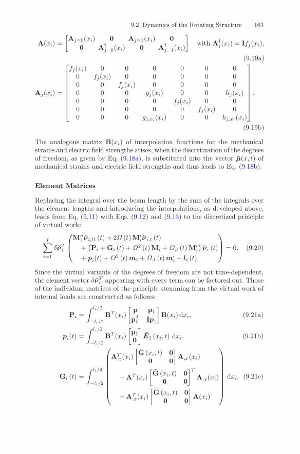
9.2 Dynamics of the Rotating Structure 163
A(xi) =[Aj=0(xi) 0 Aj=1(xi) 0
0 A†j=0(xi) 0 A†
j=1(xi)
]
with A†j(xi) = Ifj(xi),
(9.19a)
Aj(xi) =
⎡
⎢⎢⎢⎢⎢⎢⎢⎢⎣
fj(xi) 0 0 0 0 0 00 fj(xi) 0 0 0 0 00 0 fj(xi) 0 0 0 00 0 0 gj(xi) 0 0 hj(xi)0 0 0 0 fj(xi) 0 00 0 0 0 0 fj(xi) 00 0 0 gj,xi(xi) 0 0 hj,xi(xi)
⎤
⎥⎥⎥⎥⎥⎥⎥⎥⎦
.
(9.19b)
The analogous matrix B(xi) of interpolation functions for the mechanicalstrains and electric field strengths arises, when the discretization of the degreesof freedom, as given by Eq. (9.18a), is substituted into the vector μ(x, t) ofmechanical strains and electric field strengths and thus leads to Eq. (9.18b).
Element Matrices
Replacing the integral over the beam length by the sum of the integrals overthe element lengths and introducing the interpolations, as developed above,leads from Eq. (9.11) with Eqs. (9.12) and (9.13) to the discretized principleof virtual work:
I∑
i=1
δνTi
⎛
⎜⎝
M′ ′i νi,tt (t) + 2Ω (t)M′
iνi,t (t)+(Pi + Gi (t) +Ω2 (t)Mi +Ω,t (t)M′
i
)νi (t)
+ pi(t) +Ω2 (t) mi +Ω,t (t) m′i − li (t)
⎞
⎟⎠ = 0. (9.20)
Since the virtual variants of the degrees of freedom are not time-dependent,the element vector δνT
i appearing with every term can be factored out. Thoseof the individual matrices of the principle stemming from the virtual work ofinternal loads are constructed as follows:
Pi =∫ li/2
−li/2
BT (xi)[
p p†
pT† Ip†
]
B(xi) dxi, (9.21a)
pi(t) =∫ li/2
−li/2
BT (xi)[p‡0
]
E‡ (xi, t) dxi, (9.21b)
Gi (t) =∫ li/2
−li/2
⎛
⎜⎜⎜⎜⎜⎜⎜⎜⎝
AT,x(xi)
[G (xi, t) 0
0 0
]
A,x(xi)
+ AT (xi)[G (xi, t) 0
0 0
]T
A,x(xi)
+ AT,x(xi)
[G (xi, t) 0
0 0
]
A(xi)
⎞
⎟⎟⎟⎟⎟⎟⎟⎟⎠
dxi. (9.21c)

164 9 Solution Variants
The vector E‡(xi, t) of electric field strength parameters and the geometricstiffness matrices G(xi, t) and G(xi, t) take the element coordinate xi intoaccount and result from their equivalents with continuous coordinate x inconjunction with the considerations manifested in Eq. (9.17). The same holdsfor the vectors m(xi) and m′(xi), capturing the initial state inertia effects asthey appear in the remaining matrices originating from the virtual work ofexternal loads:
M′ ′i =
∫ li/2
−li/2
AT (xi)[M′ ′ 00 0
]
A(xi) dxi, li (t) =∫ li/2
−li/2
AT (xi)l (x, t) dxi,
(9.22a)
M′i =
∫ li/2
−li/2
AT (xi)[M′ 00 0
]
A(xi) dxi, m′i =
∫ li/2
−li/2
AT (xi)[m′ (xi)
0
]
dxi,
(9.22b)
Mi =∫ li/2
−li/2
AT (xi)[M 00 0
]
A(xi) dxi, mi =∫ li/2
−li/2
AT (xi)[m (xi)
0
]
dxi.
(9.22c)
All integrations may be performed symbolically. To avoid the implicationsof the effect, which might appear in the context of the description of theTimoshenko beam, a reduced integration scheme is applied, see for exampleHughes [101]. Alternatively, one may start off from four nodes per element forthe transverse displacements and rotations using cubic Lagrange polynomialsfor the interpolation and then reduce the degrees of freedom by means of astatic condensation, see Knothe and Wessels [113].
System Assembly
To set up the equations of the complete system, the boundary conditions haveto be introduced. As the beam will be clamped at the innermost node withnumber 0, the assembly of the system matrices may simply begin with nodenumber 1. Sorting the element matrices and vectors, given in Eqs. (9.21) and(9.22), into their equivalents on the system level, denoted by (
◦), allows us to
formulate the equation of motion for the system, discretized with the aid ofthe finite elements, as
M′ ′ν,tt (t) + 2Ω (t) M′ν,t (t) + PΣ (t) ν (t) = pΣ (t) . (9.23)
The constitutive properties, geometric stiffness influences, and deformation-associated inertia effects are summarized in the matrix PΣ(t), while the ap-plied loads, piezoelectric coupling implications of the electric parameters, aswell as initial state inertia effects, are joined in the vector pΣ(t):

9.2 Dynamics of the Rotating Structure 165
PΣ (t) = P + G (t) +Ω2 (t) M +Ω,t (t) M′, (9.24a)
pΣ (t) = l (t) − p (t) − Ω2 (t) m − Ω,t (t) m′. (9.24b)
Simplifications
Time-dependent system matrices are relevant only to special technical ap-plications and would require comparatively complicated solution procedures,as already pointed out in Section 8.2.2. For this reason, the general systemdescribed by Eqs. (9.23) and (9.24) will be simplified accordingly.
Remark 9.2. To assure time-independent system matrices, the angular velocityof the considered rotation is presumed to be constant and other time variantinfluences will be excluded.
Thus, the appearing angular acceleration and consequently the associatedinertia effects are eliminated:
Ω (t) = Ω = const. → Ω,t (t) = 0. (9.25)
Furthermore, the angular velocity will be incorporated into each of the con-nected matrices to facilitate a more concise formulation:
M′Ω (Ω) = 2ΩM′, MΩ (Ω) = Ω2M, mΩ (Ω) = Ω2m. (9.26)
Then the equation of motion and its compound matrix, respectively vector,given by Eqs. (9.23) and (9.24), may be rewritten for the simplified case oftime-invariant matrices, as demanded by Remark 9.2, in the following form:
M′ ′ν,tt (t) + M′Ω (Ω) ν,t (t) + PΣ (Ω) ν (t) = pΣ (t, Ω) (9.27a)
with PΣ (Ω) = P + G (Ω) + MΩ (Ω) , (9.27b)pΣ (t, Ω) = l (t) − p(t) − mΩ (Ω) . (9.27c)
9.2.3 Solution
The system of differential equations, provided by Eqs. (9.27), is of the gyro-scopic undamped type with time-invariant matrices, see Gasch and Knothe[78]. The mass matrix M′ ′ is symmetric, the gyroscopic matrix M′
Ω(Ω) isantimetric and the stiffness matrix PΣ(Ω) is symmetric as well as positivedefinite. The symmetry properties are inherited from the continuous beamdescription and become obvious, for instance, in Eqs. (8.34) by means of thematrices I, I′, I′ ′ from Eqs. (7.72). The solution to the problem at hand con-sists of three parts that are to be determined separately in the following.

166 9 Solution Variants
Steady-State Solution
The steady-state solution is concerned with the oscillation-free system, thusν,tt(t) and ν,t(t) are excluded, and the effects of the time-invariant portionof loads are retained, which are the constant applied loads, the piezoelectriccoupling implications, and the rotation induced loads:
PΣ (Ω) νs = l − p − mΩ (Ω) . (9.28)
Inversion of the overall stiffness matrix PΣ(Ω) is necessary to find the wantedsteady-state displacements, rotations, and electric potentials encapsulated inthe vector νs. Prerequisite is the determination of the initial internal loadscontained in the geometric stiffness matrix G(Ω) in accordance with Re-mark 9.2 and the considerations of Section 8.3.
Homogeneous Solution
After the separation of the steady-state solution, the natural oscillations are tobe found as the solution to the homogeneous system of differential equations.However, since the electric degrees of freedom are not associated with any-thing like the mechanical mass, all matrices except of the constitutive matrixP are singular. Therefore, the electric degrees of freedom need to be elimi-nated by means of a static condensation. Those submatrices with componentsconnected either to the mechanical or to the electrical degrees of freedom areelucidated by the additional index m, respectively e, while the index me rep-resents the coupling portions. Then the homogeneous system of differentialequations may be rewritten as
M′ ′mν∗
h,tt (t) + M′Ω;m (Ω) ν∗
h,t (t) +(PΣ;m (Ω) − PmeP−1
e PTme
)
︸ ︷︷ ︸PΣ;c(Ω)
ν∗h (t) = 0.
(9.29)For the given type, solely imaginary or solely real eigenvalues are expected,portending to either critically stable or monotonously instable behavior. Theusual exponential set-up is applied, leading to the eigenvalue problem to besolved:
ν∗h (t) = ν∗
Heλt →
(M′ ′
mλ2 + M′
Ω;m (Ω)λ+ PΣ;c (Ω))
ν∗H = 0. (9.30)
For the numerical handling, the eigenvalue problem is converted into the gen-eral form, where the upper part resembles the original problem and the lowerone delivers an identity:([
M′Ω;m (Ω) PΣ;c (Ω)
PΣ;c (Ω) 0
]
− λ[
−M′ ′m 0
0 PΣ;c (Ω)
]){λν∗
H
ν∗H
}
={00
}
. (9.31)

9.2 Dynamics of the Rotating Structure 167
As the outcome, a list of eigenvalues λk and the modal matrix H∗ with thepairwise conjugate complex eigenvectors of the general problem is obtained.Due to the normalization of the eigenvectors, the solution has to be matchedto the initial conditions. This is done when the overall solution is assembledand for this purpose the vector h∗ is provided. The homogeneous solutionthus takes the following form:
{ν∗
h,t (t)ν∗
h (t)
}
= H∗
⎡
⎢⎢⎣
. . .eλkt
. . .
⎤
⎥⎥⎦
︸ ︷︷ ︸E∗(t)
h∗. (9.32)
Since the homogeneous solution only takes the mechanical degrees of freedominto account, its vector and matrix dimensions do not match the other partsof the solution. This may be adjusted by the introduction of empty rowsand columns at the appropriate positions. To symbolize this modification, themarker (·)∗ may be dropped and Eq. (9.32) rewritten as
{νh,t (t)νh (t)
}
= HE(t)h. (9.33)
Particular Solution
At this point, the time-dependent applied loads and piezoelectric couplingimplications of the electric parameters on the right-hand side of the equationsof motion have to be taken into account:
M′ ′νp,tt (t) + M′Ω (Ω) νp,t (t) + PΣ (Ω) νp (t) = l (t) − p (t) . (9.34)
An investigation will be conducted for a mechanical or electric harmonic ex-citation with a multiple n of the rotor angular frequency Ω, where lp and pp
are the respective peak amplitudes:
l (t) − p (t) =(lp − pp
)cosnΩt =
12
(lp − pp
) (ei·nΩt + e−i·nΩt
). (9.35)
The solution approach can be handled in real or complex notation. The latteris chosen, as the system of equations to be solved is smaller and the bandedstructure of the involved matrices is sustained. Therefore, the following set-upis used:
νp(t) = ν+ei·nΩt + ν−e−i·nΩt. (9.36)
Introducing this set-up, two separate sets of equations are obtained:(
−M′ ′n2Ω2 + iM′ (Ω)nΩ + PΣ (Ω))
ν+ =12
(lp − pp
), (9.37a)
(−M′ ′n2Ω2 − iM′ (Ω)nΩ + PΣ (Ω)
)ν− =
12
(lp − pp
). (9.37b)

168 9 Solution Variants
The complex amplitude vectors ν+ and ν− are conjugates and so the solutioncan be simplified in the following way:
νp(t) = 2�(ν+ei·nΩt
). (9.38)
Solution Assembly
So far, the individual parts of the solution have been obtained and may bepieced together at this point:
{ν,t(t)ν(t)
}
={
0νs
}
+{
νh,t(t)νh(t)
}
+{
νp,t(t)νp(t)
}
. (9.39)
Still the homogeneous solution of Equation (9.33) has to be matched with theinitial conditions. Therefore, the solution at the initial point in time t0 = 0takes the following form:
{ν,t(t0)ν(t0)
}
={
0νs
}
+ Hh +{
0νp(t0)
}
. (9.40)
Isolating the hitherto undetermined vector h and substituting it back into thehomogeneous solution completes the last required step:
{νh,t(t)νh(t)
}
= HE(t)H−1
({ν,t(t0)ν(t0)
}
−{
0νs
}
−{
0νp(t0)
})
. (9.41)
10
Demonstration and Validation
The sequence of theories developed throughout the foregoing chapters, lead-ing the way from piezoelectric composites via adaptive laminated compositeshells to adaptive thin-walled beams, allows for examinations of almost ar-bitrary complexity. The attempt to provide examples for the full spectrumof capabilities will be dropped in favor of an application-oriented approach.Hence, the subsequent investigations will be carried out in view of the integralactuation of structures with certain similarity to helicopter rotor blades.
10.1 Beam Configurations
To comply with the objective of demonstration and validation, it is necessaryto engage in example configurations which, on the one hand, are as simpleas possible to warrant intelligibility and, on the other hand, retain enoughfeatures to illustrate the essential capabilities. This effort will be made inthis section, starting with the electric configuration to implement potentiallyrewarding actuation and sensing schemes.
10.1.1 Actuation and Sensing Schemes
In Section 2.5.1, the various beam actuation concepts are presented usingthe classification illustrated in Figure 2.10. Analogously applying to sensing,we distinguish between normal (lengthwise) and shear mode actuation in theplane of the wall as well as between its consistent and sectorial applicationacross the plane of the cross-section.
Wall Strain Modes
Beyond in-plane actuation and sensing associated with the normal strainε0x(x, s) and the shear strain γ0
xs(x, s) of the shell, the derived beam for-mulation is capable of analyzing the out-of-plane effects associated with the
T.H. Brockmann, Theory of Adaptive Fiber Composites,Solid Mechanics and Its Applications 161,c© Springer Science + Business Media B.V. 2009

170 10 Demonstration and Validation
bending curvature κx(x, s) and the twisting curvature ψxs(x, s) of the shell.However, with the exception of the plate strip, the actuation, respectivelysensing, effectiveness with regard to the curvatures κx(x, s) and ψxs(x, s) willbe small by virtue of the beam geometry. For this reason, no further light willbe thrown on the out-of-plane effects during subsequent examinations.
Wall Electroding Sectors
The change of the relative sign of electric field strength and polarization isassociated with the reversal of the deformation direction. To actuate or sensethe different beam deformations, the cross-section can be divided into sectorswith alternating polarization but with common electric field strength by ap-propriate interconnection of electrodes. For a clear correlation, these sectorsneed to be delimited by the relevant principal axes of the cross-section, asshown in Figure 10.1.
Fig. 10.1. Relative sign of electric field strength and polarization in the cross-sectional sectors.
Beam Schemes
The beam behavior is governed by the interplay of lay-up related wall modesand electroding specific wall sectors. For simple cross-sections, as in Fig-ure 10.1, and exposure of the walls to pure normal strain or pure shear strain,the beam behavior may be classified as described in Table 10.1. Consistentshear of the walls throughout the entire cross-section is directly related tobeam torsion. Extension of the walls in the lengthwise direction of cause cor-responds to beam extension. Normal as well as shear strains with alternatingsigns in the cross-sectional quadrants are connected to out-of-plane warpingof the cross-section. Extension and warping of both latter examples may alsobe combined with torsion by means of couplings due to the anisotropy of thewalls and the geometry of the cross-section, respectively. Similarly, couplings

10.1 Beam Configurations 171
with bending could be utilized, but are less applicable due to the unwantedimplications of the susceptibility to vibrations and external forces. The pre-ceding considerations give rise to various schemes for actuation and sensingof beam deformations.
Table 10.1. Actuation or sensing of beam deformations by virtue of strain modesand electroding sectors of the wall.
Consistent (a) 2 Sectors (b) 4 Sectors (c)
Normal Mode extension bending warpingShear Mode torsion shear warping
Example Configuration Considerations
The simultaneous consideration of actuation and sensing, as instituted by thedeveloped theory, becomes interesting as soon as a control unit is incorporatedinto the simulation. Since this would exceed the scope of the work at hand, wewill refrain from such additional complexity within the exemplary calculations.Thus, the consequences for the electrical interconnection of layers read:
Remark 10.1. A single group of electrically paralleled laminae is taken intoaccount for the example configuration.
Due to the reversibility of the piezoelectric effect and the accomplishedhomogeneous representation of mechanical and electric measures, it is suffi-cient to prove the reliability of the method for either actuation or sensing inorder to validate both.
Example Configuration Schemes
With regard to the above discussions and with the integral blade actuation forthe helicopter application in mind, as illustrated in Section 2.5, the exampleconfiguration schemes will be focused as follows:
Remark 10.2. Applicable beam schemes aiming at twist actuation will be ex-amined.
The necessary arrangements with reference to the lay-up of Figure 10.2 andthe formulations of the relative sign of electric field strength and polarizationof Eqs. (6.5) and (7.32), see also Figure 10.1, are given in Table 10.2. Thesethree actuation schemes, plus its variants, combining the different applicablecoupling and actuation types, subsequently will be implemented and theirefficiency compared.

172 10 Demonstration and Validation
Scheme I consists of two layer pairs with opposing fiber orientations and rel-ative polarizations, whereas the relative polarization around the cross-section is constant over all quadrants. Thus, it represents two pairs ofhelical windings one of which contracts while the other expands, resultingin beam twist of similar direction but compensation of beam elongation.
Scheme II consists of a central lengthwise oriented layer surrounded by a layerpair with uniform fiber orientation. With an expansion of this unidirec-tional helical winding, twist and elongation of the beam are induced inthe case of variant a. With an expansion of the lengthwise oriented fibers,elongation of the beam is achieved and complemented with twist via thepassive coupling due to the helical winding in the case of variant c. Bothmechanisms are employed simultaneously in the case of variant b. Therelative polarization around the cross-section remains constant for any ofthe variants.
Scheme III consists of two layer pairs with opposing fiber orientations andrelative polarizations. To induce warping deformation and consequentlybeam twist, the relative polarization around the cross-section alternatesfrom quadrant to quadrant. Similar results could be achieved just by usinglengthwise oriented fibers with such an alternating relative polarization.But without adjustable fiber orientations, it would not be possible toadapt to given stiffness properties, especially with regard to torsion.
Table 10.2. Actuation schemes with layup and polarization configuration for thetorsional deformation of a beam.
Wall Relative PolarizationLay-Up Layers Quadrants
Coupling Actuation Scheme H0H1
α1α2
p0 p1 p2 p(q1) p(q2) p(q3) p(q4)
none torsion I 0 −1 1 −1 1 1 1 1
torsion II a h 1 0 1 1 1 1 1 1torsion &extension
torsion &extension
II b h 1 1 1 1 1 1 1 1
extension II c h 1 1 0 0 1 1 1 1torsion &warping
warping III 0 −1 1 −1 1 −1 1 −1
10.1.2 Set-Up of Walls
Multiple layers of piezoelectric composites consisting of polymer matrix ma-terial and piezoceramic fibers form the walls of the considered beams. Theproperties of typical materials are given in Tables A.2 and A.3, respectively.For the calculations which are presented later in this chapter, the data of Epon

10.1 Beam Configurations 173
9405 resin and PZT-5H fibers is utilized. The resulting adaptive fiber com-posites are subjected to the following peak value of the electric field strength:
Ec, Ed = ±106 Vm. (10.1)
Such a fixing of the electric field strength implies the utilization of a voltagesource for the actuator application, as described in Section 4.5.
Arrangement of Fibers
The geometry on the micro-electromechanics level will be included into theupcoming elementary examinations. To confine the range of variables of theconsidered problem to the essential ones, we will abstain from analyzing detailsbeyond the fiber volume fraction ν. For a transversely isotropic layout ofcontinuous fibers, the directional fiber fractions, defined in Eqs. (5.1), thenbecome
ν1 = ν2 =√ν, ν3 = 1. (10.2)
Since the sequential stacking procedure could be shown to produce resultsof equivalent quality, see Section 5.5, with a little more flexibility and lessnumerical expenditure in comparison to the Mori–Tanaka method, it will beapplied for the example calculations. Following the discussion of Section 5.4.6,the factor c3 intended to map the disturbance of electrostatic fields close tothe electrodes will be omitted:
c3 = 0. (10.3)
To avoid the arbitrary increase of complexity without a gain of insight, thefollowing simplifications shall apply:
Remark 10.3. The composite material used for the subsequent beam configu-rations will be made of the same constituents and have identical fiber volumefractions.
Arrangement of Layers
Since the properties of the lay-up will be included in this study, a wall con-figuration has to be considered that allows for the representation of all an-ticipated effects and for the adjustment to any stiffness demand. This can beconveniently realized by a lamina in the center with fixed fiber orientationalong the beam’s lengthwise direction accompanied by two laminae on everyside. Although the developed model is capable of capturing the full rangeof anisotropic couplings, the out-of-plane effects should be excluded here toavoid blurring the results:
Remark 10.4. The beam walls to be examined will be symmetric with respectto thickness and orientation of associated layers.

174 10 Demonstration and Validation
Such a symmetric laminate, as shown in Figure 10.2, is characterized withthe aid of the layer orientation angles α0, α1 and α2 as well as the thicknessesH0, H1, and H2. For subsequent studies, fewer parameters are required andthe following simplifications are reasonable:
Remark 10.5. The fiber orientation of the center layer will be aligned with thelengthwise axis of the beam and the off-center layers will be of equal thickness.
α0 = 0, H2 = H1. (10.4)
To ease the representation, the thickness ratio h of the aligned center layerand arbitrary oriented off-center layers will be introduced as follows:
h =H0
H1. (10.5)
Fig. 10.2. Set-up of the beam wall.
10.1.3 Set-Up of Cross-Sections
The presented theory is able to cope with thin-walled beams of arbitrary cross-section. This includes highly complex configurations with any combination ofclosed cells and open branches. In the absence of correspondingly definedrequirements and since such a complexity is not necessary for the purposeof elementary examination and validation, the focus will be placed upon tworather unpretentious set-ups, see Figures 10.3 and 10.4. With regard to thecontinuity of the wall set-up, the following will be agreed:
Remark 10.6. The wall properties will be constant all around the circumfer-ential contour of the exemplary cross-sections.

10.1 Beam Configurations 175
Fig. 10.3. Characterization of a rectan-gular single-cell cross-section.
Fig. 10.4. Characterization of a con-vex double-cell cross-section.
Rectangular Single-Cell Cross-Section
The most simple case with sufficient adjustment options is the rectangularsingle-cell cross-section as depicted by Figure 10.3. To describe such a geom-etry, a separate coordinate si may be introduced with its origin in the middleof each of the four segments i of 2Si length:
si = −Si . . . Si for i = 1, 2, 3, 4 with S1 = S3 =b
2, S2 = S4 =
a
2. (10.6)
The cross-sectional dimensions of such a box beam are given by the height aand width b. Thus, the piecewise parameter representation of the wall curveassumes the following form:
y (s1) = s1, y (s2) =b
2, y (s3) = −s3, y (s4) = − b
2, (10.7a)
z (s1) =a
2, z (s2) = −s2, z (s3) = −a
2, z (s4) = s4. (10.7b)
To achieve actuation or sensing according to schemes I or II of Table 10.2, therelative sign of electric field strength and polarization needs to be constantall over the cross-section:
pc (s1) = pc (s2) = pc (s3) = pc (s4) = 1. (10.8)
To utilize the warping effect, as illustrated by scheme III of Table 10.2, therelative sign has to alternate from quadrant to quadrant of the box beam:
pd (s1 > 0) = pd (s2 < 0) = 1, pd (s2 > 0) = pd (s3 < 0) = −1, (10.9a)
pd (s3 > 0) = pd (s4 < 0) = 1, pd (s4 > 0) = pd (s1 < 0) = −1. (10.9b)

176 10 Demonstration and Validation
Convex Double-Cell Cross-Section
Further on, to consider an example with curved walls as well as multiple cells,a convex cross-section with a central web will be established, as illustrated byFigure 10.4. In this case, three segments with associated curvilinear coordi-nates are sufficient:
si = −Si . . . Si for i = 1, 2, 3 with S1 = S3 = ζR, S2 = R (1 − cos ζ) .(10.10)
The dimensions of such a cross-section may be defined via the constant ra-dius of curvature R and generating half-angle ζ. So, the piecewise parameterrepresentation of the wall curve assumes the following form:
y (s1) = R sin(s1R
), y (s2) = 0, y (s3) = −R sin
(s3R
), (10.11a)
z (s1) = R(cos
(s1R
)− cos ζ
), z (s2) = s2, z (s3) = −R
(cos
(s3R
)− cos ζ
).
(10.11b)
To achieve actuation or sensing according to schemes I or II of Table 10.2, therelative sign of electric field strength and polarization needs to be constantaround the circumference of the cross-section:
pc (s1) = pc (s3) = 1. (10.12)
To utilize the warping effect, as illustrated by scheme III of Table 10.2, therelative sign has to alternate from quadrant to quadrant of the convex cross-section:
pd (s1 > 0) = 1, pd (s3 < 0) = −1, (10.13a)pd (s3 > 0) = 1, pd (s1 < 0) = −1. (10.13b)
Due to its alignment with a principal axis, the web of the considered cross-section is free of warping influences:
pc (s2) = 0. (10.14)
10.1.4 Constitutive Coefficients
The properties of the beam cross-section are manifested in the constitutivecoefficients as given in their general formulation in Section 8.1.3. Subsequently,we will briefly illustrate, how they are obtained.
General Procedure
Due to the symmetry of the wall set-up, as demanded in Remark 10.4, thoseshell stiffness coefficients in charge of the coupling between in-plane and out-of-plane behavior vanish. By virtue of Remark 10.6, the properties of the

10.1 Beam Configurations 177
beam wall may be drawn out of the cross-sectional integrals. Further on, thelatter may be split and consequently solved with the aid of the piecewiserepresentations of the wall curves and the sectorial description of the relativeelectroding sign of Table 10.2.
Specific Illustration
For clarity, the printout of the results will be confined to the simple box beamof Eqs. (10.7). For the immediate, respectively later, use in order to ease therepresentation, the following ratios characterizing the box-beam geometry willbe introduced:
na/b =a
b, nX/b =
X
b. (10.15)
Then the beam stiffness coefficients, depending on the shell stiffnesses associ-ated with lengthwise extension and bending from Eqs. (8.7), become
P11 = 2A11
(1 + na/b
)b, (10.16a)
P55 =A11
6(3 + na/b
)n2
a/bb3 + 2D11b, (10.16b)
P66 =A11
6(1 + 3na/b
)b3 + 2D11na/bb, (10.16c)
P77 =A11
24(1 − na/b)2
1 + na/bn2
a/bb5 +
D11
6(1 + na/b
) (n2
a/b − na/b + 1)b3. (10.16d)
Correspondingly, the beam stiffness coefficients, depending on the shell stiff-nesses associated with shear and twist from Eqs. (8.8), take the followingform:
P22 = 2A33b, P33 = 2A33na/bb, (10.16e)
P44 = 2A33
n2a/b
1 + na/bb3 + 8D33
(1 + na/b
)b. (10.16f)
Those non-zero beam stiffness coefficients, depending on the shell stiffnessesassociated with the coupling between lengthwise extension and shear, read
P14 = −2A13na/bb2, P25 = A13na/bb
2, P36 = A13na/bb2. (10.16g)
With regard to the electromechanical coefficients of the beam, two differentcases need to be distinguished. For schemes I and II of Table 10.2 with con-sistent electric conditions around the cross-section, given by Eqs. (10.8), thefollowing coefficients are applicable:
P18 = 2Ac14
(1 + na/b
)b, P48 = −2Ac
34na/bb2, P88 = 2Ac
44
(1 + na/b
)b.
(10.16h)

178 10 Demonstration and Validation
For scheme III with changes in the electric sign between adjacent quadrants,as described by Eqs. (10.9), the electromechanical coefficients of the beambecome
P79 = − Ad14
4(1 − na/b)2
1 + na/bna/bb
3, P99 = 2Ad44
(1 + na/b
)b. (10.16i)
Since there is no need for simultaneous actuation with different schemes andthus the number of groups of electrically paralleled laminae has been limitedto one in Remark 10.1, either Eqs. (10.16h) or (10.16i) are defined for theexample at hand.
10.2 Elementary Examinations
The goal of these examinations is, on the one hand, to gain some insight intothe behavior of beams with adaptive fiber composites and, on the other, toderive an optimal configuration for the numerical studies following in Sec-tion 10.3. The starting point is the analytic solution regarding the statics ofthe non-rotating structure as developed in Section 9.1. With the helicopterapplication in view, special attention is given to the torsion problem. Unrea-sonable complication should to be avoided at this stage of analysis by virtueof the following restriction:
Remark 10.7. These examinations are carried out by means of the box beamas described by Eqs. (10.16) and will be limited to the membrane response ofEq. (6.20).
10.2.1 Beam Geometry Influences on the Actuation Schemes
With regard to the actuation capabilities, the solution to the beam torsionproblem, as given by Eq. (9.4), contains two different parts indicated by theconstants �twist and �warp. The prior is in charge of direct and extension-coupled twist, schemes I and II of Table 10.2, and the latter of warping-coupled twist, scheme III of Table 10.2. The influence of the overall beamgeometry on the efficiency of the actuation schemes will be analyzed on thisbasis.
Solution in Terms of Characteristic Ratios
Besides the geometric ratios of Eq. (10.15), the passive and active constitu-tive coefficients of the beam wall may be represented with reference to thelengthwise shell stiffness as follows:
a13 =A13
A11, a33 =
A33
A11, ac
14 =Ac14
A11, ac
34 =Ac34
A11, ad
14 =Ad14
A11.
(10.17)

10.2 Elementary Examinations 179
With these stiffness ratios and the limitation to membrane response, as statedin Remark 10.7, the dimensionless constants �twist and �warp from Eqs. (9.5b)as well as the decay-length parameter λ from Eq. (9.7) can be rewritten as
�twist = −nX/b
1 + na/b
na/b
ac34 − a13ac
14
a33 − a213
Ec, �warp = −6n2
X/b
na/bad14E
d, (10.18a)
λ = 4nX/b
1 − na/b
√
3 (a33 − a213). (10.18b)
While the otherwise unchanged functions η1(ξ) and η0(ξ) of Eqs. (9.6) makeuse of the above decay-length parameter λ, the complete solution for the beamtwist due to actuation without the implications of external loads reduces fromEq. (9.4) to
φ (ξ) = − (ξ − η1 (ξ)) �twist + η0 (ξ) �warp. (10.19)
The first term represents the direct and extension-coupled torsion with aprincipally linear distribution along the beam length, disturbed by the non-linear influences of the warping effect comprised in the function η1(ξ). Thesecond term captures the warping-coupled torsion with its non-linear behaviordescribed by the function η0(ξ).
Geometry Influence Discussion
Keeping all the constitutive ratios of Eqs. (10.17) as well as the appearingelectric field strength values constant, while varying the geometric ratios ofEqs. (10.15), allows for the anticipated examination of the efficiency of thedifferent actuation schemes. For the graphical representations to be displayedsubsequently, the rotation induced at the beam tip is normalized via divi-sion by the maximum result within the considered ranges of the two beamaspect ratios. For direct and extension-coupled twist, schemes I and II ofTable 10.2, the first term of the solution in Eq. (10.19) applies and is shownin Figure 10.5. As it was to be expected, the influence of the ratio nX/b ispredominantly linear. Hence, the longer the beam is dimensioned, the greaterthe tip rotation becomes. Further on, the deviation of cross-sectional aspectratio na/b from unity results for fixed wall properties in a reduction of thetorsional stiffness and thus serves as an explanation for the increase of thetip twist. For warping-coupled twist, scheme III of Table 10.2, the secondterm of the solution in Eq. (10.19) is relevant and plotted in Figure 10.6.Regarding the cross-sectional aspect ratio na/b, the argumentation with thetorsional stiffness in this case should similarly hold. Since the quadratic oc-currences of the ratio nX/b, within the constant �warp and in the denominatorof the function η0(ξ), cancel each other out, there is hardly any influence ofthe relative beam length visible in the examined range of values. The onlywarping restraint of the configuration at hand is located at the clamped endof the beam. It is the source for a non-vanishing rate of twist and consequently

180 10 Demonstration and Validation
the warping coupling. Its influence may be slightly enlarged by an increase inthe beam length. Alternatively, this could give rise to segmented designs withseveral warping restraints.
Fig. 10.5. Geometry influence on thedirect and extension-coupled twist actu-ation (normalized).
Fig. 10.6. Geometry influence on thewarping-coupled twist actuation (nor-malized).
10.2.2 Beam Property Adaptation
To obtain results within the same order of magnitude as expected from theinitially given application example of helicopter rotor blades, the data of anexisting main rotor system will be utilized. The corresponding diagonal entriesP11 to P66 of the beam stiffness matrix are given in Table B.1 for the BO105 ofBolkow/MBB/Eurocopter. The characteristic ratios regarding geometry andstiffness of the box beam will now be fitted as far as possible to the real-life example. Although such an agreement of properties is rather insignificantfor the numerical validation, some premises might be formulated to definethe configuration. First of all, the torsional stiffness should match, since it isclosely related to the major objective of these examinations. Then, however,the stiffness request in the lengthwise direction of the beam cannot be fulfilled.Furthermore, one additional deviation has to be accepted:
Remark 10.8. The tensional stiffness P11 and the chordwise shear stiffness P22
are accepted to exhibit deviations from the application example data.
Cross-Sectional Aspect Ratio
Division of the shear stiffness coefficients of the beam, see Eq. (10.16e), byeach other directly yields the cross-sectional aspect ratio
na/b =P33
P22. (10.20)
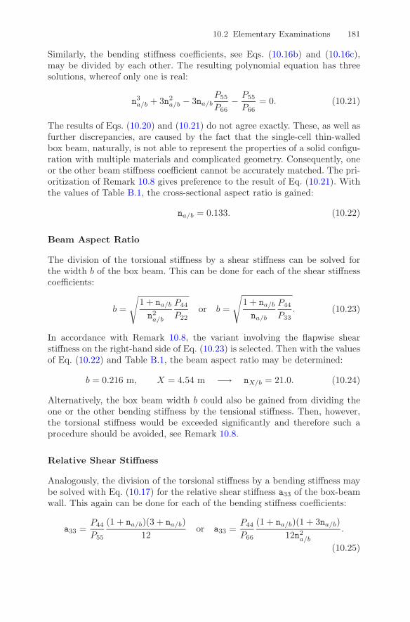
10.2 Elementary Examinations 181
Similarly, the bending stiffness coefficients, see Eqs. (10.16b) and (10.16c),may be divided by each other. The resulting polynomial equation has threesolutions, whereof only one is real:
n3a/b + 3n2
a/b − 3na/bP55
P66− P55
P66= 0. (10.21)
The results of Eqs. (10.20) and (10.21) do not agree exactly. These, as well asfurther discrepancies, are caused by the fact that the single-cell thin-walledbox beam, naturally, is not able to represent the properties of a solid configu-ration with multiple materials and complicated geometry. Consequently, oneor the other beam stiffness coefficient cannot be accurately matched. The pri-oritization of Remark 10.8 gives preference to the result of Eq. (10.21). Withthe values of Table B.1, the cross-sectional aspect ratio is gained:
na/b = 0.133. (10.22)
Beam Aspect Ratio
The division of the torsional stiffness by a shear stiffness can be solved forthe width b of the box beam. This can be done for each of the shear stiffnesscoefficients:
b =
√1 + na/b
n2a/b
P44
P22or b =
√1 + na/b
na/b
P44
P33. (10.23)
In accordance with Remark 10.8, the variant involving the flapwise shearstiffness on the right-hand side of Eq. (10.23) is selected. Then with the valuesof Eq. (10.22) and Table B.1, the beam aspect ratio may be determined:
b = 0.216 m, X = 4.54 m −→ nX/b = 21.0. (10.24)
Alternatively, the box beam width b could also be gained from dividing theone or the other bending stiffness by the tensional stiffness. Then, however,the torsional stiffness would be exceeded significantly and therefore such aprocedure should be avoided, see Remark 10.8.
Relative Shear Stiffness
Analogously, the division of the torsional stiffness by a bending stiffness maybe solved with Eq. (10.17) for the relative shear stiffness a33 of the box-beamwall. This again can be done for each of the bending stiffness coefficients:
a33 =P44
P55
(1 + na/b)(3 + na/b)12
or a33 =P44
P66
(1 + na/b)(1 + 3na/b)12n2
a/b
.
(10.25)

182 10 Demonstration and Validation
Since the relationship between the stiffness coefficients P55 and P66 has beenutilized to establish the cross-sectional aspect ratio na/b in Eq. (10.22), bothvariants of Eq. (10.25) with the values of Table B.1 provide identical results:
a33 = 0.210. (10.26)
Deviation Contemplations
With the characteristic ratios obtained above, it may now be possible to checkhow large the deviations tolerated by Remark 10.8 are. The shell stiffness co-efficients A11 and A33 can be determined by substitution of Eqs. (10.23) andsubsequently Eq. (10.22) into those beam stiffness coefficients of Eqs. (10.16),which are exactly kept and contain the respective shell stiffness coefficientsto be solved for. Thus, all diagonal entries of the beam stiffness matrix canbe calculated as given in Table 10.3 together with the deviations from the ex-ample application data, see Table B.1. The great discrepancy in the tensionalstiffness P11 is due to the fact that the thin-walled box beam is not able toemploy fibers close to its neutral axis, where they would primarily contributeto the tensional stiffness.
Table 10.3. Diagonal entries of the beam stiffness matrix resulting from the prop-erty adaptation with deviations from the application example data, see Table B.1.
Coefficient Units Value Deviation
P11 106 N 36.1 −50.5 %P22 106 N 6.71 +8.58 %P33 106 N 0.89 0P44 103 Nm2 4.85 0P55 103 Nm2 6.82 0P66 103 Nm2 173 0P77 Nm4 16.8
10.2.3 Wall Geometry Optimization
On the one hand, the relative coupling stiffness a13 of the box-beam wall re-quiring knowledge about one of the coupling coefficients of the beam stiffnessmatrix and, on the other hand, those ratios of Eq. (10.17) representing theadaptive properties, are not prescribed. These remnants of the box-beam con-figuration will be specified through the study of the following optimizationproblem:
Remark 10.9. Optimize the box-beam configuration with the objective of at-taining maximum tip twist in consideration of the different actuation schemeswhile satisfying the stiffness and geometry constraints of Section 10.2.2.
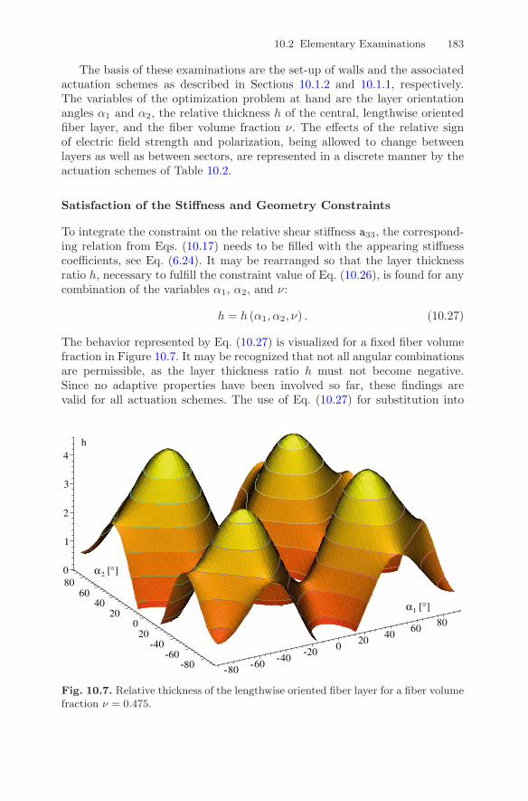
10.2 Elementary Examinations 183
The basis of these examinations are the set-up of walls and the associatedactuation schemes as described in Sections 10.1.2 and 10.1.1, respectively.The variables of the optimization problem at hand are the layer orientationangles α1 and α2, the relative thickness h of the central, lengthwise orientedfiber layer, and the fiber volume fraction ν. The effects of the relative signof electric field strength and polarization, being allowed to change betweenlayers as well as between sectors, are represented in a discrete manner by theactuation schemes of Table 10.2.
Satisfaction of the Stiffness and Geometry Constraints
To integrate the constraint on the relative shear stiffness a33, the correspond-ing relation from Eqs. (10.17) needs to be filled with the appearing stiffnesscoefficients, see Eq. (6.24). It may be rearranged so that the layer thicknessratio h, necessary to fulfill the constraint value of Eq. (10.26), is found for anycombination of the variables α1, α2, and ν:
h = h (α1, α2, ν) . (10.27)
The behavior represented by Eq. (10.27) is visualized for a fixed fiber volumefraction in Figure 10.7. It may be recognized that not all angular combinationsare permissible, as the layer thickness ratio h must not become negative.Since no adaptive properties have been involved so far, these findings arevalid for all actuation schemes. The use of Eq. (10.27) for substitution into
Fig. 10.7. Relative thickness of the lengthwise oriented fiber layer for a fiber volumefraction ν = 0.475.

184 10 Demonstration and Validation
the objective function guarantees the satisfaction of the stiffness constraintand eliminates the variable h. The geometry constraints of Eqs. (10.22) and(10.24) are directly inserted.
Compilation of the Objective Function
The objective function of this optimization problem is the evaluation of thetwist solution, being given by Eq. (10.19) in conjunction with Eqs. (10.17)and (10.18), at the free end of the beam. For the constitutive coefficientsappearing in the respective ratios, the relative layer thickness h of Eq. (10.27)is required besides the material properties and the particular actuation schemeconfiguration from Table 10.2. After introduction of the geometry constraints,specified in Eqs. (10.22) and (10.24), the tip twist may be found for anycombination of the variables α1, α2, and ν:
φ = φ (α1, α2, ν, ξ = 1) . (10.28)
The behavior represented by Eq. (10.28) is exemplarily visualized for thecases of direct twist actuation (scheme I of Table 10.2) in Figure 10.8 andcombined actuation of coupled extension and twist (scheme IIb of Table 10.2)in Figure 10.9 for a fixed fiber volume fraction.
Fig. 10.8. Beam tip rotation due to direct twist actuation for a fiber volume fractionν = 0.475.
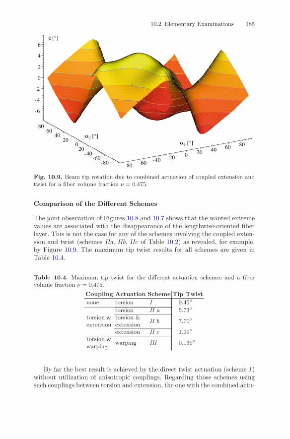
10.2 Elementary Examinations 185
Fig. 10.9. Beam tip rotation due to combined actuation of coupled extension andtwist for a fiber volume fraction ν = 0.475.
Comparison of the Different Schemes
The joint observation of Figures 10.8 and 10.7 shows that the wanted extremevalues are associated with the disappearance of the lengthwise-oriented fiberlayer. This is not the case for any of the schemes involving the coupled exten-sion and twist (schemes IIa, IIb, IIc of Table 10.2) as revealed, for example,by Figure 10.9. The maximum tip twist results for all schemes are given inTable 10.4.
Table 10.4. Maximum tip twist for the different actuation schemes and a fibervolume fraction ν = 0.475.
Coupling Actuation Scheme Tip Twist
none torsion I 9.45◦
torsion II a 5.73◦
torsion &extension
torsion &extension
II b 7.70◦
extension II c 1.99◦
torsion &warping
warping III 0.139◦
By far the best result is achieved by the direct twist actuation (scheme I )without utilization of anisotropic couplings. Regarding those schemes usingsuch couplings between torsion and extension, the one with the combined actu-

186 10 Demonstration and Validation
ation of the helical wound as well as the lengthwise oriented fibers (scheme IIb)is superior to the pure variants. It does not involve passive fibers and, con-sequently, there is no need for surmounting the associated stiffness. Activewarping torsion is not able to provide any similar results for this exampleconfiguration with a decay-length parameter λ ≈ 70. Further on, the imple-mentation would be more expensive due to the necessary segmented electrod-ing. Nevertheless, the efficiency improves for comparatively short beams, asit is visible by comparing Figures 10.5 and 10.6 as well as by examining thefunction η0(ξ) in Figure 9.1.
Influence of the Fiber Volume Fraction
All the results shown above have been calculated for a fiber volume fractionν = 0.475. This value represents the optimum for the direct twist actuationand is very close to the optima of the other schemes. In Figure 10.10, thedependence of tip twist as well as layer orientation and thickness is exemplarilydepicted for the direct twist scheme. The layer thicknessH1 therein is obtainedby taking the formulation for one of the exactly preserved stiffness coefficientsof the example rotor blade, see Remark 10.8 and Table 10.3, supplying itwith all the known constitutive and configurative data, and solving it for therequired value. As obvious here but applicable also for the other cases, it isfound that the influence of the fiber volume fraction is rather good-natured,confirming the calculations with a collective value of the fiber volume fraction.
Fig. 10.10. Influence of the fiber volume fraction on the necessary layer orientationand thickness as well as on the resulting tip twist for the direct twist actuation.

10.3 Validation and Evaluation 187
10.3 Validation and Evaluation
While the analytical solution limited to the static problem has been applied atleast in a simplified fashion for the elementary examinations of Section 10.2,the finite element solution capable of capturing the general problem has notyet been employed. Both solution variants will now be checked against eachother and against an entirely independent approach with a commercial finiteelement software.
10.3.1 Reference Configurations
Again, the exemplary application data of the BO105 rotor system of Table B.1will be employed. Thus, a beam of length X, clamped perpendicularly to theaxis of rotation at the radius X, is rotating with the angular velocity Ω. Forthe sake of simplicity, the precone angle as well as the angle of attack, includedin the presented theory, are not put into operation. Since we have abstainedfrom modeling the complexity associated with the blade attachment, the dy-namic response results cannot be expected to be comparable to those of a realhelicopter. Dissimilar to the considerations of Section 10.2, with the mem-brane response assumption of Remark 10.7, the shell representation may nowbe taken into account. Besides the already used geometry of the rectangularsingle-cell cross-section, the analysis will be extended to the convex double-cellcross-section, both being described in Section 10.1.3.
Rectangular Single-Cell Cross-Section
The most efficient configuration resulting from the optimization will beadopted for the subsequent calculations. This, namely, has been the directtwist actuation (scheme I of Tables 10.2 and 10.4). The relevant specifica-tions concerning the geometry of the cross-section are given by Eqs. (10.22)and (10.24) or may be gathered for the wall set-up from Figure 10.10:
α1 = −α2 = −17.6◦, H1 = 1.82 mm. (10.29)
On this basis, the complete set of constitutive coefficients of the beam canbe calculated according to Eqs. (10.16). Due to the symmetric lay-up withbalanced layer orientation of the selected scheme, the walls do not exhibit anycoupling between the lengthwise extension and shear (A13 = 0). Consequently,the beam neither possesses couplings between extension and torsion (P14 = 0)nor between bending and shear (P25, P36 = 0). The remaining, non-vanishingcoefficients are given for the two reduced shell response variants in Table 10.5together with the relative deviations from membrane response as considered inTable 10.3. The enhanced calculation using the shell description without cross-sectional loads, Eqs. (6.22), leads to a stiffening of the affected coefficients byless than one percent. On the contrary, the shell description without cross-sectional strains, Eqs. (6.23), shows greater deviations since it is valid only for

188 10 Demonstration and Validation
the rather special case where any contraction or expansion of the cross-sectionis counteracted, for example, by an internal pressurization of the beam.
Table 10.5. Constitutive properties of the exemplary beam configuration with rec-tangular single-cell cross-section.
Shell without Cross-SectionalLoads, see Eq. (6.22) Strains, see Eq. (6.23)
Coefficient Units Value Deviation [%] Value Deviation [%]
P11 106 N 36.1 0 41.2 +12.2P22 106 N 6.71 0 6.71 0P33 106 N 0.890 0 0.890 0P44 103 Nm2 4.88 +0.70 4.88 0P55 103 Nm2 6.85 +0.52 7.81 +12.7P66 103 Nm2 173 +0.00 197 +12.2P77 Nm4 17.0 +0.82 19.3 +12.9P48 10−3 Nm
V0.178 0 0.178 0
P88 10−12 Nm2
V2 11.4 0 11.4 0
Convex Double-Cell Cross-Section
The curved cross-section is divided by a central web into two cells. The as-sociated geometric description is given by Eqs. (10.10) and (10.11). On thisbasis, the radius of curvature R and generating half-angle ζ may be expressedin terms of the beam width b and the ratio na/b between the extents alongthe cross-sectional axes:
y (s1 = S1) = R sin ζ = b2 ,
z (s1 = 0) = R (1 − cos ζ) = na/bb2
−→ tan ζ =2na/b
1 + n2a/b
, R =1 + n2
a/b
4na/bb.
(10.30)Although such a shape still is symmetric with regard to both principal axes,adaptation of beam properties and optimization of wall geometry cannot beaccomplished with such simple measures as available for the box beam. Notto exceed the scope of the work at hand, here we will desist from the thrillsof sophisticated optimization procedures; elementary literature is provided byCollatz and Wetterling [55] or Pierre [141]. Since convex cross-section andairfoil profile are similar to a certain extent, the blade chord b will be utilizeddirectly, as given by Table B.1. Together with arbitrary fixing of the cross-sectional aspect ratio na/b, the generating half-angle ζ and radius of curvatureR, according to Eq. (10.30), read as follows:
b = 0.27 m, na/b = 0.155 −→ ζ = 17.6◦, R = 0.446 m. (10.31)
In Remarks 10.3 to 10.6, the wall properties around the circumferential con-tour have been specified. For the central web, however, an altered configura-tion may be selected. In the beam property adaptation of Section 10.2.2 for

10.3 Validation and Evaluation 189
the rectangular single-cell cross-section, it has not been possible to get close tothe tensional stiffness of the example application data due to the lack of fibersclose to the neutral axis. This can be improved by furnishing the web withpurely lengthwise oriented fibers with the greatest possible stiffness. To com-ply with the assumption of thin walls, included in Remark 6.4, the thickness ofthe web will be limited to 1/10 of its height. Adding tensional stiffness to thecenter of the cross-section requires a reduction around the contour and thusallows for a thinner skin and/or increased fiber angle. Such a configuration ofthe wall geometry is given in the following.
Web: H0 = 4.19 mm, H1 = 0 mm, (10.32a)Skin: H0 = 0 mm, H1 = 0.55 mm, α1 = −α2 = 22.5◦. (10.32b)
Using high modulus carbon fibers for the web, see Table A.1, the geometryspecified by Eqs. (10.31) and (10.32) leads to the beam properties given inTable 10.6 being approximately within the same order of magnitude of theexample application data, see Table B.1. Unlike the case of the box beam, thecouplings between bending and shear (P25, P36) do not only depend on thecoupling of lengthwise extension and shear (A13 = 0) but also on the bendingand twist (D13 �= 0) of the outer wall. Such effects, however, are beyond thescope of the membrane response assumption. Due to the limited thickness ofthe web, the selected configuration shows only a minor increase in the tensionalstiffness. Further on, the centered web aligned with one cross-sectional axis isnot able to fully depict the influence pertaining to the both axes as exertedin real life by a solid spar.
10.3.2 Reference Calculations
The stiffening due to the assumption of a cross-section without strains, respec-tively curvatures, in its plane visible in the right-hand columns of Tables 10.5and 10.6, has been found to be not very realistic. Hence, the subsequent cal-culations will be conducted by means of the assumption of a cross-sectionwithout loads in its plane. The results obtained for such a shell descriptionof the beam walls are, furthermore, to be compared to the outcome of thesignificantly simpler membrane description. As briefly mentioned in the intro-duction to this section, three different solution approaches will be examined.The associated individual restrictions are discussed in the following.
Analytic Approach
Within the bounds of the underlying theory, the analytic solution derivedin Section 9.1 can be regarded as exact. It is confined to the statics of thenon-rotating structure as well as certain constitutive couplings and load con-figurations. Special cases, like the elongation of the rotating beam due tocentrifugal forces, may be simulated with the appropriate choice of loads.

190 10 Demonstration and Validation
Table 10.6. Constitutive properties of the exemplary beam configuration with con-vex double-cell cross-section.
Shell without Cross-SectionalMembrane, Loads, Strains,
Coefficient Units see Eq. (6.20) see Eq. (6.22) see Eq. (6.23)
P11 106 N 39.2 39.2 44.2P22 106 N 6.17 6.17 6.17P33 106 N 0.929 0.929 0.929P44 103 Nm2 4.84 4.86 4.86P55 103 Nm2 6.81 6.81 7.98P66 103 Nm2 77.3 77.3 107.8P77 Nm4 0.798 0.822 1.14P25 Nm 0 0.827 1.11P36 Nm 0 0.0264 0.0355P48 10−3 Nm
V0.172 0.172 0.172
P88 10−12 Nm2
V2 6.31 6.31 6.31
Beam Finite Elements
Due to the discretization and interpolation, the finite element method is cate-gorized as an approximation. The corresponding details are shown throughoutthe course of derivation of the beam finite element solution in Section 9.2.With identical underlying theory but without all the restrictions necessary toobtain an analytical solution, it is able provide answers to a wide range ofproblems.
Shell Finite Elements
As outlined in Section 4.2.5, the implementation of anisotropic thermal effectsin commercial finite element codes may be utilized to simulate the implicationsof the piezoelectric effect. To capture the behavior of thin-walled beams withcross-sections as defined above, spatial shell elements may be employed. Withthis methodology, however, it is not possible to examine problems with dy-namic actuation. The beams with rectangular and convex cross-sections havebeen discretized with 2200, respectively 2300, SHELL99 elements of ANSYSas exemplarily shown for the latter case in Figure 10.11.
10.3.3 Static Behavior
Since neither the analytic approach nor the application of shell finite elementsis able to handle the general problem of dynamic actuation and response in therotating environment, the developed beam finite elements need to be counter-checked by means of the individual solution components, see Section 9.2.3.

10.3 Validation and Evaluation 191
Fig. 10.11. Discretization of the convex cross-section beam with shell finite ele-ments.
Beam Extension due to Centrifugal Forces
First, the steady-state solution with the elongation of the blade resulting fromthe centrifugal forces will be examined. The formulation for the analyticalapproach is provided by Eq. (9.8). The required linear and constant portionsof the line force n(x) in the lengthwise direction depicting the centrifugaleffects are
nx = mΩ2, nx = nxX. (10.33)
The contained constant m represents mass per length of the beam. For the twodifferent cross-sections under consideration, it takes the following form.
Rectangular cross-section: m = 8(1 + na/b
)bH1ρ, (10.34a)
Convex cross-section: m = 4ζR4H1ρskin
+ 2 (1 − cos ζ)RH0ρweb
. (10.34b)
Although the stiffness properties are largely similar, the total masses of thetwo beam variants differ significantly due to the diversity of construction andmaterials. While the single-cell rectangular cross-section possesses a mass of33.8 kg, the double-cell convex cross-section beam gets by with only 20.0 kg.The beam elongation in response to the centrifugal force field is shown for thedifferent calculation approaches in Table 10.7. Since both beams are free ofextension torsion coupling (P14 = 0), no plate properties are involved in thesolution to the lengthwise displacement, see Eqs. (9.8) and (8.7a). Therefore,the comparison of the two analytic variants cannot show any divergence to beinduced by the membrane response assumption. Both finite element solutionsare very close to each other and show only minor deviations to the analyticalsolution. Therewith, the vector of centrifugal forces mΩ(Ω) as well as thelongitudinal components of the beam stiffness matrix PΣ(Ω) of Eqs. (9.27)and (9.28), respectively, are successfully checked.

192 10 Demonstration and Validation
Table 10.7. Beam extension due to centrifugal forces.
Rect. Single-Cell Conv. Double-Cellu (ξ = 1) Error u (ξ = 1) Error
Method Shell Assumption [cm] [%] [cm] [%]
analytic no cross-sec. loads, Eq. (6.22) 1.4204 0.7760membrane response, Eq. (6.20) 1.4204 0 0.7760 0
beam FE no cross-sec. loads, Eq. (6.22) 1.4252 +0.34 0.7774 +0.18shell FE ANSYS SHELL99 1.4245 +0.30 0.7817 +0.74
Beam Torsion due to Piezoelectric Coupling
Next, a constant electric field will be applied to the piezoelectric compositeswithin the non-rotating structure to verify the constant factor of the piezo-electric actuation vector p(t) as well as the torsional components of the beamstiffness matrix PΣ(Ω). This is done in consideration of the warping effectwith cubic Hermite shape functions and without the warping effect using lin-ear Lagrange polynomials, see Section 9.2.2. The first shows good agreementwith the exact analytical solution and the shell finite element model, while inthe latter case the torsional rigidity is notably smaller due to abandonmentof the warping restraint at the clamped end. Naturally, the actuation vectorsin both cases are identical. The values of the resulting blade tip rotation aregiven in Table 10.8.
Table 10.8. Beam torsion due to piezoelectric coupling.
Rect. Single-Cell Conv. Double-Cellφ(ξ = 1) Error φ(ξ = 1) Error
Method Shell Assumption [◦] [%] [◦] [%]
analytic no cross-sec. loads, Eq. (6.22) 9.4479 9.1983membrane response, Eq. (6.20) 9.4484 +0.01 9.1987 +0.00
beam FE no cross-sec. loads, Eq. (6.22) 9.4184 −0.31 9.2076 +0.10— ” —, without warping 9.5436 +1.01 9.2408 +0.46
shell FE ANSYS SHELL99 9.4584 +0.11 9.2185 +0.22
Different from above, plate properties (D33) are involved in the solution tothe twisting angle, see Eqs. (9.4), (9.5), and (8.8c). Due to the closed cross-sections and thin walls, the implications of the membrane response assumptionare very small for the cases at hand. However, this changes drastically withthe consideration of open cross-section topologies just as well covered by thedeveloped theory, where the torsional stiffness (P44) of the beam is solelygoverned by the twisting stiffness (D33) of the walls. As an example, the boxbeam subjected to piezoelectrically induced torsion is shown for the shell finiteelement approach in Figure 10.12. Close to the clamped end, the influence ofthe warping restraint on the beam twist becomes visible.

10.3 Validation and Evaluation 193
Fig. 10.12. Torsion of the rectangular cross-section beam via piezoelectric coupling.
10.3.4 Free Vibrations
Since the essential parts of the right-hand side of the differential equationsystem, given by Eqs. (9.27), have demonstrated their operability, the homo-geneous solution will be examined in detail to complete the inspection of theleft-hand side. As there is no analytic approach available to capture the dy-namic behavior, the subsequent comparison comprises the formulations withthe developed beam finite elements and with the commercial shell finite el-ements. The resulting natural frequencies ω for all modes up to the thirdtorsional mode are given in Table 10.9 for the non-rotating system as well asin Table 10.10 for the rotating system.
Table 10.9. Natural angular frequencies of the non-rotating systems.
ω[1/s] Rect. Single-Cell Conv. Double-CellMode Shape Beam FE Shell FE Beam FE Shell FE
1st lead-lag 25.92 25.88 22.56 22.61
2nd lead-lag 159.39 158.69 139.79 139.81
3rd lead-lag 433.67 430.11 384.80 383.51
1st flap 5.17 5.16 6.70 6.72
2nd flap 32.28 31.92 41.84 41.82
3rd flap 89.80 87.37 116.42 115.08
4th flap 174.33 164.96 226.13 217.91
5th flap 284.84 258.11 369.70 340.62
6th flap 419.67 357.34 545.08 470.48
7th flap 577.01 452.55 750.04 569.63
1st torsion 127.36 121.84 148.89 145.25
2nd torsion 382.69 314.74 446.71 372.29
3rd torsion 639.82 424.57 744.63 491.20

194 10 Demonstration and Validation
Table 10.10. Natural angular frequencies of the rotating systems.
ω[1/s] Rect. Single-Cell Conv. Double-CellMode Shape Beam FE Shell FE Beam FE Shell FE
1st lead-lag 34.73 34.99 32.27 32.53
2nd lead-lag 193.13 192.98 177.46 177.86
3rd lead-lag 473.34 470.79 428.97 428.58
1st flap 48.23 48.41 48.92 48.93
2nd flap 121.18 120.61 124.58 123.32
3rd flap 210.86 208.71 225.04 217.71
4th flap 323.10 315.72 355.98 330.90
5th flap 456.24 435.27 515.80 453.23
1st torsion 127.07 138.17 148.64 154.21
2nd torsion 382.59 342.50 446.63 382.56
3rd torsion 639.82 471.60 744.58 508.03
Influence of the Rotation
Comparing the natural frequencies of the non-rotating and rotating system,consistently reveals a moderate increase for the lead-lag modes and a steepincrease for the flapping modes. The deviating imprints of the rotational stiff-ening are founded on the significantly dissimilar structural stiffness proper-ties with regard to the respective cross-sectional axis. This behavior is alsobeing reflected in the associated mode shapes as visible in the example of Fig-ure 10.13 for the fifth bending mode shape of the rectangular cross-sectionbeam and Figure 10.14 for the third lead-lag mode shape of the convexcross-section beam. With the increase of beam internal loads towards thecenter of rotation, the oscillation amplitudes decrease, while the wavelengthis stretched. For the developed beam finite elements, such effects are capturedby virtue of the second-order theory of Section 8.3. Its derivation, however,does not indicate similar effects for either rotation or warping, see Eq. 8.39.Consequently, frequencies as well as shapes of the torsional modes are notsensitive to rotation in the beam finite element model. In contrast, the shellfinite element model shows at least a small dependence.
Fig. 10.13. Fifth flapping mode of the rectangular cross-section beam for the non-rotating (light) and rotating (dark) system (beam finite elements).
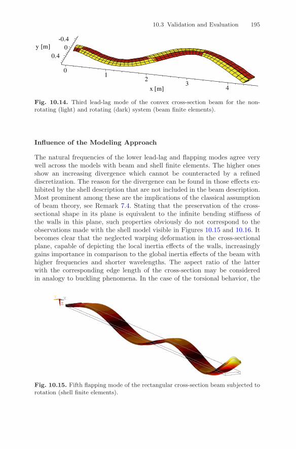
10.3 Validation and Evaluation 195
Fig. 10.14. Third lead-lag mode of the convex cross-section beam for the non-rotating (light) and rotating (dark) system (beam finite elements).
Influence of the Modeling Approach
The natural frequencies of the lower lead-lag and flapping modes agree verywell across the models with beam and shell finite elements. The higher onesshow an increasing divergence which cannot be counteracted by a refineddiscretization. The reason for the divergence can be found in those effects ex-hibited by the shell description that are not included in the beam description.Most prominent among these are the implications of the classical assumptionof beam theory, see Remark 7.4. Stating that the preservation of the cross-sectional shape in its plane is equivalent to the infinite bending stiffness ofthe walls in this plane, such properties obviously do not correspond to theobservations made with the shell model visible in Figures 10.15 and 10.16. Itbecomes clear that the neglected warping deformation in the cross-sectionalplane, capable of depicting the local inertia effects of the walls, increasinglygains importance in comparison to the global inertia effects of the beam withhigher frequencies and shorter wavelengths. The aspect ratio of the latterwith the corresponding edge length of the cross-section may be consideredin analogy to buckling phenomena. In the case of the torsional behavior, the
Fig. 10.15. Fifth flapping mode of the rectangular cross-section beam subjected torotation (shell finite elements).

196 10 Demonstration and Validation
discrepancy of the natural frequencies with ascending mode shapes is evenmore articulate. The considered warping displacements are confined to pro-portionality with the twist rate and to the direction out of the cross-sectionalplane, see Remarks 7.3 and 7.4 leading to Eq. (7.11). Just like in the case ofthe lead-lag and flapping modes, there are no means of accounting for localinertia effects of the walls and resulting decrease of natural frequencies. In Fig-ures 10.17 and 10.18, the cross-sectional deformations are already noticeablefor the first torsional mode but become excessive for the third torsional mode.In addition to relatively thin walls, both example configurations possess veryslim cross-sections being fairly disadvantageous in this context.
Fig. 10.16. Fifth flapping mode of the convex cross-section beam subjected torotation (shell finite elements).
Fig. 10.17. First and third torsionalmodes of the rectangular cross-sectionbeam not subjected to rotation (shell fi-nite elements).
Fig. 10.18. First and third torsionalmodes of the convex cross-section beamnot subjected to rotation (shell finite el-ements).

10.3 Validation and Evaluation 197
Influence of the Cross-Section
In all cases, the agreement of beam and shell finite element results for theconvex double-cell cross-section is superior to the rectangular single-cell cross-section. On the one hand, the outer walls of the first are thinner and thusmore flexible, but on the other hand, they contribute only a part of the totalmass. Further on, the convex shape and particularly the stiff web, stabilizethe cross-sectional shape. Consequently, the beam with a convex double-cellcross-section is less sensitive to the influence of the local inertia effects ofthe walls in comparison to the global inertia effects of the beam. Moreover,the not yet explicitly mentioned discrepancy of beam and shell finite elementresults for the first torsional mode as well as the rotation dependence of nat-ural frequencies for torsional mode shapes in the shell model, are diminishedwith the convex double-cell cross-section. Therefore, it is permissible to con-clude that the discovered deviations on the whole are due to the differenthandling of the cross-section with the use of beam and shell finite elementsrespectively. So which of these two modeling approaches is more appropriate?As always, there are two faces to the truth. Regarding the results in corre-spondence with the input data, the shell representation, presuming properimplementation, is clearly more precise. However, the input data already rep-resents an idealization, since the actual structure, which in the given exampleis equipped with a foam core and thus is prevented from noticeable defor-mations of the cross-sectional shape, has been replaced by its thin-walledlikeness. To conclude, further pieces of the beam stiffness matrix PΣ(Ω) aswell as mass matrix M′ ′ and gyroscopic matrix M′
Ω(Ω) may be regarded asvalidated.
10.3.5 Forced Vibrations
As far as available, the counter-check of individual solution components, seeSection 9.2.3, has been successfully completed in Sections 10.3.3 and 10.3.4.The developed beam finite elements may now be employed for their propri-etary task of simulating the universal dynamic behavior of adaptive thin-walled beams. In the most general case, the developed theory is able to de-scribe the mechanical as well as the electric response to combined mechanicaland electric excitation. In the context of Remark 10.1, the example config-uration has been simplified to handle either actuation or sensing and withthe helicopter rotor blade application in mind, the prior has been pursued.So finally, the response of the rotating beam to a piezoelectrically inducedtwist actuation will be sought. To visualize the result, the twist angle ofthe last node is selected from the overall solution of Eq. (9.41) and dis-played over time in Figure 10.19. Since the harmonic excitation with thethreefold of the rotor angular frequency is close to the frequency of the firsttorsional mode of the employed box beam, the plot shows the characteristicbeat pattern. With this last step, the three-dimensional dynamic behavior of
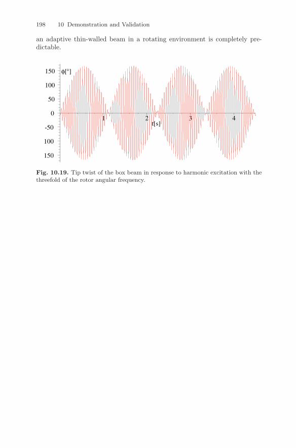
198 10 Demonstration and Validation
an adaptive thin-walled beam in a rotating environment is completely pre-dictable.
Fig. 10.19. Tip twist of the box beam in response to harmonic excitation with thethreefold of the rotor angular frequency.

11
Conclusion
In this final chapter, we will attempt to review the findings attained duringthe various steps of theory derivation and subsequent validation as well as topresent the prospect of potential future development.
11.1 Summary
Adaptive fiber composites have been examined on the basis of a thorough,systematic treatment of the theory across a wide spectrum from piezoelectricmaterial behavior to the dynamics of rotating structures. Making a pointof consistency and continuity, the derived formulations are accompanied byseveral innovations and improvements, the most relevant of which will berecalled below:
• Extension of Dirichlet’s principle of minimum potential energy to electro-mechanically coupled problems.
• Deduction of simplifying assumptions for piezoelectric materials in consid-eration of spatial extent and electroding configuration via examination ofassociated implications on spatial field distributions.
• Proposition of an enhanced micro-electromechanical model to determinethe constitutive properties of piezoelectric composites based on the se-quential stacking of constituents with uniform fields.
• Derivation of a comprehensive description of composite shells with piezo-electric layers in arbitrary configuration for possibly combined actuationand sensing.
• Development of a novel theory for thin-walled beams with arbitrary cross-sections incorporating more than the usual membrane properties withoutadditional degrees of freedom.
• Consideration of shear flexibility, torsional warping, and electromechanicalcoupling as well as of rotational effects by virtue of including an extendedset of second-order terms.
T.H. Brockmann, Theory of Adaptive Fiber Composites,Solid Mechanics and Its Applications 161,c© Springer Science + Business Media B.V. 2009
200 11 Conclusion
• Derivation of an analytic solution to gain insight into the static behaviorof structures with adaptive capabilities and to be used for adjustment andoptimization of beam configurations.
• Derivation of a general solution via the formulation of spatial beam finiteelements, accounting for arbitrary combinations of actuator and sensorapplications with voltage and current source, respectively measurement,to capture the dynamic behavior of the rotating structure.
To ensure the soundness of the various assumptions and simplifications madethroughout the course of derivation as well as to exclude errors in the imple-mentation, the obtained results have been successfully counterchecked usingcompletely independent approaches. Therein, the following steps are regarded,in particular:
• Validation of the micro-electromechanical model for piezoelectric compos-ites with the aid of experimental and finite element modeling results avail-able in the literature.
• Validation of the beam finite elements by comparison of solution compo-nents to those attainable with commercial shell finite elements for exampleconfigurations with a rectangular single-cell and a convex double-cell cross-section approximating the properties of an actual helicopter rotor blade.
Using the presented comprehensive formulation of the theoretical frameworkand the associated elementary examinations, the recognition and utilization ofcausal relationships, in view of the manipulation of structural behavior withadaptive means, is facilitated. With the resulting spatial beam finite elements,a versatile modeling tool can be provided as a basis for further investigations.
11.2 Perspective
The focus of this work is directed towards the structural aspects of adaptivesystems with associated actuation and sensing capabilities. The consequen-tial next step therefore would be to consider the linkage with various controlmodels to make the abilities of the complete system accessible. With regardto the application case of helicopter rotor blades, coupling with an aerody-namics model would allow us to perform the aeroelastic analyses necessary toprove the effectiveness of the concept. Furthermore, noise emission and im-pact on the environment might be simulated by means of an acoustics model.To enhance the comparability of the developed adaptive thin-walled beamrepresentation with the real rotor system, it could be refined with additionalfeatures, like pre-twist, non-rigid blade mounting, or cyclic pitch to cover for-ward flight conditions. Another direction for the extension of the developedtheory is the incorporation of alternative constitutive models to take othermultifunctional materials into account. This could be interesting, especiallyfor the example of composites with electromechanical coupling through carbonnanotubes.

11.2 Perspective 201
To ensure correctness of the partially complex derivation, the symbolicmathematics software Maple has been employed for each and every step, in-cluding implementation of the beam finite elements. The numeric computa-tions could be carried out with the support of integrated routines from thelibrary of the Numerical Algorithms Group (NAG). Nevertheless, the compu-tational performance and, moreover, the user-friendliness have never surpassedthe level of a development tool. Therefore, an implementation involving fastequation-solvers and an easy-to-use interface is advisable. This could be ac-complished, for instance, through the extension of an existing finite elementor multi-body dynamics code, which in addition would allow for combinationwith a variety of other elements. While the presented example calculationshave so far revealed only a touch of the genuine capabilities, such a softwarewould enable the comfortable accomplishment of comprehensive design stud-ies. The results to be obtained therewith should be put into practice with theconstruction of test specimens and be compared to the ensuing experimentalresults.

A
Material Properties
Table A.1. Properties of the applied reinforcement material.
Carbon Fibers, Ref. [116]Units Stiffness Constants Engineering Constants
109 Nm2 C11 = C22 20.0 E1 = E2 15.0
C12 9.98 E3 232C13 = C23 6.45 G13 = G23 5.01C33 235 G12 24.0C44 = C55 24.0 ν13 = ν23 0.0139C66 5.01 ν12 0.495
103 kgm3 Density ρ 1.8∗
Table A.2. Properties of polymer materials.
Araldite D Araldite 2020 Epon 9405Constants Units Ref. [49] Ref. [169] prod. data
C11 = C22 = C33 109 Nm2 8.0 7.28 4.57
C12 = C13 = C23 4.4 4.46 2.46C44 = C55 = C66 1.8 1.41 1.05
E1 = E2 = E3 109 Nm2 4.88 3.89 2.85
ν12 = ν13 = ν23 0.35 0.38 0.35∗
ε11ε0
= ε22ε0
= ε33ε0
4 5 4∗
ρ 103 kgm3 1.161
∗ estimated
T.H. Brockmann, Theory of Adaptive Fiber Composites,Solid Mechanics and Its Applications 161,c© Springer Science + Business Media B.V. 2009

204 A Material Properties
Table A.3. Properties of piezoelectric materials.
PZT-5A PZT-5H PZT-7A PMN-30%PTConstants Units Ref. [20] Ref. [20] Ref. [19] Ref. [186]
CE11 = CE
22 109 Nm2 121 126 148 117
CE12 75.4 79.5 76.2 103
CE13 = CE
23 75.2 84.1 74.2 101CE
33 111 117 131 108CE
44 = CE55 21.1 23.0 25.3 71
CE66 22.6 23.5 36.0 66
SE11 = SE
22 10−12 m2
N16.4 16.5 10.7 52.0
SE12 −5.74 −4.78 −3.2 −18.9
SE13 = SE
23 −7.22 −8.45 −4.6 −31.1SE
33 18.8 20.7 13.9 67.7SE
44 = SE55 47.5 43.5 39.4 14.0
SE66 44.3 42.6 27.8 15.2
EE1 = EE
2 109 Nm2 61.5 60.0 95.0 19.3
EE3 53.4 48.2 81.9 15.3
GE13 = GE
23 21.1 23.0 25.3 71.0GE
12 22.6 23.5 36.0 66.0
νE13 = νE
23 0.441 0.510 0.384 0.581νE12 0.349 0.291 0.322 0.379
e31 = e32N
Vm−5.4 −6.55 −2.11 −2.4
e33 15.8 23.3 9.5 27.1e15 = e24 12.3 17.0 9.2 13.6
d31 = d32 10−12 mV
−171 −274 −60 −921d33 374 593 150 1981d15 = d24 584 741 362 190εε11ε0
=εε22ε0
916 1700 460 3307εε33ε0
830 1470 235 1242
εσ11ε0
=εσ22ε0
1730 3130 840 3600εσ33ε0
1700 3400 425 7800
ρ 103 kgm3 7.75 7.5 7.6 8.04
TCP◦C 365 193 350
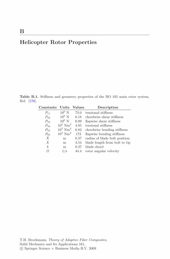
B
Helicopter Rotor Properties
Table B.1. Stiffness and geometry properties of the BO 105 main rotor system,Ref. [170].
Constants Units Values Description
P11 106 N 73.0 tensional stiffnessP22 106 N 6.18 chordwise shear stiffnessP33 106 N 0.89 flapwise shear stiffnessP44 103 Nm2 4.85 torsional stiffnessP55 103 Nm2 6.82 chordwise bending stiffnessP66 103 Nm2 173 flapwise bending stiffnessX m 0.37 radius of blade bolt positionX m 4.54 blade length from bolt to tipb m 0.27 blade chordΩ 1/s 44.4 rotor angular velocity
T.H. Brockmann, Theory of Adaptive Fiber Composites,Solid Mechanics and Its Applications 161,c© Springer Science + Business Media B.V. 2009

References
[1] J. Aboudi, Mechanics of Composite Materials—A Unified MicromechanicalApproach. Studies in Applied Mechanics (Elsevier Science Publishers, Ams-terdam, 1991)
[2] J. Aboudi, Micromechanical prediction of the effective coefficients of thermo-piezoelectric multiphase composites. J. Intell. Mater. Syst. Struct. 9, 713–722(1998)
[3] K. Adachi, G. Park, D.J. Inman, Shunting macro-fiber composite actuator forstructural damping, in Noise and Vibration Engineering: Proceedings of ISMA2002, ed. by P. Sas, B. Van Hal (Katholieke Universiteit Leuven, Leuven, 2002),pp. 411–419
[4] H. Allik, T.J.R. Hughes, Finite element method for piezoelectric vibration. Int.J. Numer. Methods Eng. 2, 151–157 (1970)
[5] M. Allongue, H.J. Marze, F. Potdevin, The quiet helicopter—from research toreality, in Proceedings of the American Helicopter Society 55th Annual Forum(American Helicopter Society, Montreal, 1999)
[6] H. Altenbach, J. Altenbach, R. Rikards, Einfuhrung in die Mechanik derLaminat- und Sandwichtragwerke (Deutscher Verlag fur Grundstoffindustrie,Stuttgart, 1996)
[7] E.A. Armanios, A.M. Badir, Free vibration analysis of anisotropic thin-walledclosed-section beams. AIAA J. 33(10), 1905–1910 (1995)
[8] H. Banno, Recent developments of piezoelectric ceramic products and compos-ites of synthetic rubber and piezoelectric ceramic particles. Ferroelectrics 50,3–12 (1983)
[9] W. Becker, D. Gross, Mechanik elastischer Korper und Strukturen (Springer,Berlin, 2002)
[10] W. Beckert, W.S. Kreher, Modelling piezoelectric modules with interdigitatedelectrode structures. Comput. Mater. Sci. 26, 36–45 (2003)
[11] W. Beitz, K.H. Kuttner, Dubbel—Taschenbuch fur den Maschinenbau,14th edn. (Springer, Berlin, 1981)
[12] A. Benjeddou, J.F. Deu, S. Letombe, Free vibrations of simply-supportedpiezoelectric adaptive plates: An exact sandwich formulation. Thin-WalledStruct. 40, 573–593 (2002)
T.H. Brockmann, Theory of Adaptive Fiber Composites,Solid Mechanics and Its Applications 161,c© Springer Science + Business Media B.V. 2009
208 References
[13] A.A. Bent, Active fiber composites for structural actuation. Ph.D. Thesis,Massachusetts Inst. of Tech. (1997)
[14] A.A. Bent, N.W. Hagood, Improved performance in piezoelectric fiber compos-ites using interdigitated electrodes, in Smart Structures and Materials 1995:Smart Materials, ed. by A.P. Jardine. Proceedings of SPIE, vol. 2441 (SPIE,Bellingham, 1995), pp. 196–212
[15] A.A. Bent, N.W. Hagood, Piezoelectric fiber composites with interdigitatedelectrodes. J. Intell. Mater. Syst. Struct. 8, 903–919 (1997)
[16] A.A. Bent, N.W. Hagood, J.P. Rodgers, Anisotropic actuation with piezoelec-tric fiber composites, in Proceedings of the 4th International Conference onAdaptive Structures and Technologies, Cologne, Germany (CRC Press, BocaRaton, 1993), pp. 418–433
[17] A.A. Bent, N.W. Hagood, J.P. Rodgers, Anisotropic actuation with piezoelec-tric fiber composites. J. Intell. Mater. Syst. Struct. 6(3), 338–349 (1995)
[18] Y. Benveniste, A new approach to the application of Mori–Tanaka’s theory incomposite materials. Mech. Mater. 6, 147–157 (1987)
[19] D. Berlincourt, H.H.A. Krueger, Properties of specialized Clevite ceramics.Technical Report TP-232, Morgan Electro Ceramics
[20] D. Berlincourt, H.H.A. Krueger, C. Near, Properties of piezoelectricity ceram-ics. Technical Report TP-226, Morgan Electro Ceramics
[21] R.L. Bielawa, Rotary Wing Structural Dynamics and Aeroelasticity. AIAA Ed-ucation Series (American Institute of Aeronautics and Astronautics, Washing-ton, 1992)
[22] E.R. Booth, M.L. Wilbur, Acoustic aspects of active-twist rotor control, inProceeding of the American Helicopter Society 58th Annual Forum (AmericanHelicopter Society, Montreal, 2002)
[23] A.R.S. Bramwell, G. Done, D. Balmford, Bramwell’s Helicopter Dynamics(Butterworth Heinemann, Oxford, 2001)
[24] R. Bredt, Kritische Bemerkungen zur Drehungselastizitat. Z. Ver. Dtsch. Ing.40, 785 (1896)
[25] K.S. Brentner, F. Farassat, Helicopter noise prediction: The current status andfuture direction. J. Sound Vib. 170(1), 79–96 (1994)
[26] T.H. Brockmann, R. Lammering, An analytic approach to piezoelectric fibercomposites—from micromechanics modeling to beam behavior. Z. Angew.Math. Mech. 81(2), 281–282 (2001)
[27] T.H. Brockmann, R. Lammering, Analysis of piezoelectric fiber compositebeams, in Smart Structures and Materials 2001: Smart Structures and Inte-grated Systems, ed. by L. Porter Davies. Proceedings of SPIE, vol. 4327 (SPIE,Bellingham, 2001), pp. 460–471
[28] T.H. Brockmann, R. Lammering, Analysis of piezoelectric fiber compositestructures and finite element validation, in Solids, Structures, and CoupledProblems in Engineering: Proceedings of ECCM 2001, ed. by Z. Waszczyszyn,J. Pamin (Vesalius, Cracow, 2001)
[29] T.H. Brockmann, R. Lammering, An analytic approach to piezoelectric fibercomposites—design study of active beams with closed cross-sections. Proc.Appl. Math. Mech. 1(1), 139–140 (2002)
[30] T.H. Brockmann, R. Lammering, Dynamics of rotating piezoelectric fiber com-posite beams, in Noise and Vibration Engineering: Proceedings of ISMA 2002,ed. by P. Sas, B. Van Hal (Katholieke Universiteit Leuven, Leuven, 2002),pp. 167–176

References 209
[31] T.H. Brockmann, R. Lammering, Adaptive concepts to reduce noise and vi-brations of helicopter rotors, in Anwendungen der Akustik in der Wehrtechnik,ed. by B. Nolte (Studiengesellschaft der DWT, Bonn, 2002), pp. 12–26
[32] T.H. Brockmann, R. Lammering, Active damping of helicopter rotor bladeswith piezoelectric fiber composites, in Second International Workshop onDamping Technologies: Materials and Devices for the Next Decade (Univer-siteit Stellenbosch, Stellenbosch, 2003)
[33] T.H. Brockmann, R. Lammering, Finite beam elements for rotating piezoelec-tric fiber composite structures, in Computational Fluid and Solid Mechanics2003, ed. by K.J. Bathe (Elsevier, Amsterdam, 2003)
[34] T.H. Brockmann, R. Lammering, Helicopter rotor blade dynamics with adap-tive fiber composites, in Jahrbuch 2004 der Deutschen Gesellschaft Fur Luft-und Raumfahrt Lilienthal-Oberth e.V. (DGLR, Bonn, 2004)
[35] T.H. Brockmann, R. Lammering, Beam finite elements for rotating piezoelec-tric fiber composite structures. J. Intell. Mater. Syst. Struct. 17(5), 431–448(2006)
[36] T.H. Brockmann, R. Lammering, F. Yang, Modelling and computational analy-sis of structures with integrated piezoelectric material, in Proceedings of the IIECCOMAS Thematic Conference on Smart Structures and Materials, ed. byC.A. Mota Soares (ECCOMAS, Lisbon, 2005)
[37] T.H. Brockmann, R. Lammering, F. Yang, Modelling and computational analy-sis of structures with integrated piezoelectric material. Mech. Adv. Mater.Struct. 13(5), 371–378 (2006)
[38] G. Brunk, M. Kraska, Tensorrechnung. Technische Universitat Berlin, Institutfur Mechanik (1998)
[39] A. Budo, Theoretische Mechanik. Hochschulbucher fur Physik (VEB DeutscherVerlag der Wissenschaften, Berlin, 1974)
[40] A. Buter, Untersuchung adaptiver Konzepte zur Reduktion von Hubschrauber-vibrationen, zur Minderung des Hubschrauberlarms und zur Steigerung deraerodynamischen Effizienz. Ph.D. Thesis, RWTH, Aachen, DLR Braunschweig(1998)
[41] W.G. Cady, Piezoelectricity—An Introduction to the Theory and Applicationsof Electromechanical Phenomena in Crystals (Dover, New York, 1964)
[42] B.J. Cannon, D. Brei, Feasibility study of microfabrication by coextrusion(MFCX) hollows fibers for active composites. J. Intell. Mater. Syst. Struct.11, 659–670 (2000)
[43] M.J. Carpenter, Using energy methods to derive beam finite elements incorpo-rating piezoelectric materials. J. Intell. Mater. Syst. Struct. 8, 26–40 (1997)
[44] C.E.S. Cesnik, Wing shape deformation for high-performance aerial vehicles.ICASE Morphing Seminar Series. Presentation (2002)
[45] C.E.S. Cesnik, R. Palacios, Modeling piezocomposite actuators embedded inslender structures, in 44th AIAA/ASME/ASCE/AHS Structures, StructuralDynamics, and Materials Conference. AIAA, vol. 2003-1803 (AIAA, Norfolk,2003).
[46] C.E.S. Cesnik, S.J. Shin, On the modeling of integrally actuated helicopterblades. Int. J. Solids Struct. 38(10–13), 1765–1789 (2001)
[47] C.E.S. Cesnik, S. Shin, W.K. Wilkie, M.L. Wilbur, P.H. Mirick, Modeling, de-sign, and testing of the NASA/Army/MIT active twist rotor prototype blade,in Proceedings of the American Helicopter Society 55th Annual Forum (AHS,Montreal, 1999).
210 References
[48] C.E.S. Cesnik, S.J. Shin, M.L. Wilbur, Dynamic response of active twist rotorblades. Smart Mater. Struct. 10(1), 62–76 (2001)
[49] H.L.W. Chan, J. Unsworth, Simple model for piezoelectric Ceramic/Polymer1–3 composites used in ultrasonic transducer applications. IEEE Trans. Ultra-son., Ferroelectr. Freq. Control 36(4), 434–441 (1989)
[50] K.K. Chawla, Composite Materials—Science and Engineering (Springer, NewYork, 1998)
[51] P.C. Chen, I. Chopra, A feasibility study to build a smart rotor: Induced-strainactuation of airfoil twisting using piezoceramic crystals, in Smart Structuresand Intelligent Systems (Proceedings), vol. 1917 (SPIE, Bellingham, 1993),pp. 238–254
[52] P.C. Chen, I. Chopra, Hover testing of smart rotor with induced-strain actua-tion of blade twist. AIAA J. 35(1), 6–16 (1997)
[53] I. Chopra, Review of state of art of smart structures and integrated systems.AIAA J. 40(11), 2145–2187 (2002)
[54] R.M. Christensen, Mechanics of Composite Materials (Wiley, New York, 1979)[55] L. Collatz, W. Wetterling, Optimierungsaufgaben. Heidelberger Taschenbucher
(Springer, Berlin, 1971)[56] R. Courant, D. Hilbert, Methoden der Mathematischen Physik, vols. 1 & 2
(Springer, Berlin, 1968)[57] B.N. Cox, G. Flanagan, Handbook of analytical methods for textile composites.
Technical Report NASA Contractor Report 4750, NASA Langley ResearchCenter (1997)
[58] E.F. Crawley, K.B. Lazarus, Induced strain actuation of isotropic andanisotropic plates. AIAA J. 29(6), 944–951 (1991)
[59] J. Curie, P. Curie, Developpement, par pression, de l’electricite polaire dansles cristaux hemiedres a faces inclinees. C. R. Hebd. Seances Acad. Sci. 91,294–295 (1880)
[60] J. Curie, P. Curie, Sur l’electricite polaire dans les cristaux hemiedres a facesinclinees. C. R. Hebd. Seances Acad. Sci. 91, 383–386 (1880)
[61] W.F. Deeg, The analysis of dislocation, crack, and inclusion problems in piezo-electric solids. Ph.D. Thesis, Stanford University (1980)
[62] M.M. Denn, Optimization by Variational Methods (McGraw-Hill Book Com-pany, New York, 1969)
[63] B. Domke, Aviation images, www.b-domke.de/AviationImages.html (2002)[64] L.H. Donnell, Stability of thin-walled tubes under torsion. Technical Report
NACA Report No. 479, National Advisory Committee for Aeronautics (1933)[65] A.J. Du Plessis, N. Hagood, Modeling and experimental testing of twist actu-
ated single cell composite beams for helicopter blade control. Master’s Thesis,Massachusetts Inst. of Tech. (1996)
[66] M.L. Dunn, M. Taya, An analysis of piezoelectric composite materials contain-ing ellipsoidal inhomogenities. Proc. R. Soc. Lond. A 443, 265–287 (1993)
[67] M.L. Dunn, M. Taya, Micromechanics predictions of the effective electroelasticmoduli of piezoelectric composites. Int. J. Solids Struct. 30(2), 161–175 (1993)
[68] G.J. Dvorak, M.V. Srinivas, New estimates of overall properties of heteroge-neous solids. J. Mech. Phys. Solids 47, 899–920 (1999)
[69] C.L. Dym, Introduction to the Theory of Shells (Pergamon, Oxford, 1974)[70] C.L. Dym, I.H. Shames, Solid Mechanics: A Variational Approach. Advanced
Engineering Series (McGraw-Hill Book Company, New York, 1973)

References 211
[71] B. Edwards, C. Cox, Revolutionary concepts for helicopter noise reduction—S.I.L.E.N.T. program. Technical Report CR-2002-211650, NASA, Langley Re-search Center (2002)
[72] J.E. Elspass, M. Flemming, Aktive Funktionsbauweisen (Springer, Berlin,1998)
[73] J.D. Eshelby, The determination of the elastic field of an ellipsoidal inclusion,and related problems. Proc. R. Soc. Lond. A 241, 376–396 (1957)
[74] J. Fischer, Elektrodynamik: Ein Lehrbuch (Springer, Berlin, 1976)[75] G. Floquet, Sur les equations differentielles lineaires a coefficients periodiques.
Ann. Ec. Norm. 12(2), 37–89 (1883)[76] B.D. Freed, V. Babuska, Finite element modeling of composite piezoelectric
structures with MSC/NASTRAN, in Smart Structures and Materials 1997:Smart Structures and Integrated Systems. Proceedings of SPIE, vol. 3041(SPIE, Bellingham, 1997), pp. 676–688
[77] P. Funk, Variationsrechnung und ihre Anwendung in Physik und Technik, 2ndedn. Die Grundlehren der mathematischen Wissenschaften in Einzeldarstel-lung, vol. 94 (Springer, Berlin, 1970)
[78] R. Gasch, K. Knothe, Strukturdynamik, vols. 1 & 2 (Springer, Berlin, 1987 &1989)
[79] W. Gembler, Leise Hubschrauber Zelle, Abschlußbericht 20 H 95 07 A. EU-ROCOPTER Deutschland GmbH (1999)
[80] M. Gerardin, D. Rixen, Parametrization of finite rotations in computationaldynamics: A review. Rev. Europ. Elem. Finis 4, 497–553 (1995)
[81] K. Ghandi, N.W. Hagood, Nonlinear modeling and characterisation techniquesfor phase transition in electro-mechanically coupled devices. Ph.D. Thesis,Massachusetts Inst. of Tech. (1998)
[82] G.L. Ghiringhelli, P. Masarati, P. Mantegazza, Analysis of an Actively TwistedRotor by Multi-Body Global Modeling. ASME Mechanics and Materials Con-ference (Blacksburg, Virginia, 1999)
[83] C. Giacovazzo, Fundamentals of Crystallography (Oxford University Press,London, 2002)
[84] K. Girkmann, Flachentragwerke—Einfuhrung in die Elastostatik der Scheiben,Platten, Schalen und Faltwerken, 6th edn. (Springer, Wien, 1963)
[85] A. Gjelsvik, The Theory of Thin-Walled Bars (Wiley, New York, 1981)[86] H. Goldstein, Klassische Mechanik, 3rd edn. (Akademische Verlagsgesellschaft,
Frankfurt am Main, 1974)[87] S.V. Gopinathan, V.V. Varadan, V.K. Varadan, A review and critique of the-
ories for piezoelectric laminates. Smart Mater. Struct. 9, 24–48 (2000)[88] A.E. Green, W. Zerna, Theoretical Elasticity (Oxford University Press, London,
1975)[89] F. Gruttmann, R. Sauer, W. Wagner, A geometric nonlinear eccentric 3D-beam
element with arbitrary cross-section. Comput. Methods Appl. Mech. Eng. 160,383–400 (1998)
[90] N. Hagood, R. Kindel, K. Ghandi, P. Gaudenzi, Improving transverse actuationof piezoceramics using interdigitated surface electrodes, in Smart Structuresand Materials 1993: Smart Structures and Intelligent Systems, ed. by M.E.Regelbrugge. Proceedings of SPIE, vol. 1917 (SPIE, Bellingham 1993), pp. 341–352

212 References
[91] W.G. Hankel, Elektrische Untersuchungen. XV. Abhandlung: Ueber die aktino-und piezoelektrischen Eigenschaften des Bergkrystalles und ihre Beziehung zuden thermoelektrischen. Abhandlungen der koniglich sachsischen Gesellschaftder Wissenschaften, vol. 12(20) (Hirzel, Leipzig, 1881)
[92] J. Helbig, W. Glaubitt, H. Spaniol, P. Vierhaus, U. Lange, R. Hansch,W. Watzka, D. Sporn, Development and technology of doped sol-gel derivedlead zirconate titanate fibers. Smart Mater. Struct. 12, 987–992 (2003)
[93] S. Heo, J.H. Kim, Y.Y. Kim, Significance of distortion in thin-walled closedbeam section design. Int. J. Solids Struct. 40, 633–648 (2003)
[94] J.W. High, W.K. Wilkie, Method for fabricating NASA-standard macro-fibercomposite piezoelectric actuators. Technical Report NASA/TM-2003-212427,NASA (2003)
[95] G.W. Hill, On the part of the motion of the linear perigee which is a functionof the mean motions of the sun and moon. Acta Math. 8, 1–36 (1886)
[96] D.H. Hodges, Review of composite rotor blade modeling. AIAA J. 28(3), 561–565 (1990)
[97] D.H. Hodges, A mixed variational formulation based on exact intrinsic equa-tions for dynamics of moving beams. Int. J. Solids Struct. 26(11), 1253–1273(1990)
[98] D.H. Hodges, E.H. Dowell, Nonlinear equations of motion for the elastic bend-ing and torsion of twisted nonuniform rotor blades. NASA Technical NoteNASA TN D-7818, National Aeronautics and Space Administration, Wash-ington DC (1974)
[99] N.J. Hoff, The accuracy of Donnell’s equation. J. Appl. Mech. 22, 329–334(1955)
[100] R. Holland, E.P. EerNisse, Variational evaluation of admittances of multielec-troded three-dimensional piezoelectric structures. IEEE Trans. Sonics Ultra-son. 15, 119–132 (1968)
[101] T.J.R. Hughes, The Finite Element Method (Prentice-Hall, Englewood Cliffs,1987)
[102] A. Huxley, Brave New World (Chatto and Windus, London, 1932)[103] T. Ikeda, Fundamentals of Piezoelectricity (Oxford University Press, London,
1990)[104] Institute of Electrical and Electronics Engineers. Standard on Piezoelectricity,
Std 176-1978 (IEEE, New York, 1978)[105] M. Itskov, Tensor Algebra and Tensor Analysis for Engineers—With Applica-
tions to Continuum Mechanics (Springer, Berlin, 2007)[106] H. Janocha (ed.), Adaptronics and Smart Structures—Basics, Materials, De-
sign, and Applications (Springer, Berlin, 1999)[107] R.M. Jones, Mechanics of Composite Materials (Scripta Book Company, Wash-
ington, 1975)[108] S.N. Jung, V.T. Nagaraj, I. Chopra, Refined structural model for thin- and
thick-walled composite rotor blades. AIAA J. 40(1), 105–116 (2002)[109] M. Kamlah, Ferroelectric and ferroelastic piezoceramics—modeling of electro-
mechanical hysteresis phenomena. Contin. Mech. Thermodyn. 13(4), 219–268(2001)
[110] K.R.V. Kaza, R.G. Kvaternik, Nonlinear aeroelastic equations for combinedflapwise bending, chordwise bending, torsion, and extension of twisted nonuni-form blades in forward flight. Technical Memorandum TM 74059, NASA(1977)

References 213
[111] J. Kempner, Remarks on Donnell’s equations. J. Appl. Mech. 22, 117–118(1955)
[112] V. Kloppel, B. Enenkel, et al., ADASYS I—Adaptives dynamisches System furHubschrauber, Abschlußbericht 20 H 99 06 A. EUROCOPTER DeutschlandGmbH (2001)
[113] K. Knothe, H. Wessels, Finite Elemente—Eine Einfuhrung fur Ingenieure(Springer, Berlin, 1999)
[114] W.T. Koiter, A consistent first approximation in the general theory of thinelastic shells, in Proceedings of the Symposium on the Theory of Thin Elas-tic Shells, ed. by W. Koiter. Internation Union of Theoretical and AppliedMechanics (North-Holland, Amsterdam, 1960), pp. 12–33
[115] P. Konstanzer, Decentralized vibration control for active helicopter rotor blades.Ph.D. Thesis, Universitat Stuttgart, Stuttgart, Germany (2002)
[116] R.D. Kriz, W.S. Stinchcomb, Elastic moduli of transversely isotropic fibers andtheir composites. Exp. Mech. 19, 41–49 (1979)
[117] D.L. Kunz, Survey and comparison of engineering beam theories for helicopterrotor blades. J. Aircr. 31(3), 473–478 (1994)
[118] C. Lanczos, The Variational Principles of Mechanics. Mathematical Exposi-tions (University of Toronto Press, Toronto, 1977)
[119] P.D. Lax, Linear Algebra and Its Applications, 2nd edn. Pure and AppliedMathematics (Wiley-Interscience, New York, 2007)
[120] G. Lehner, Elektromagnetische Feldtheorie fur Ingenieure und Physiker(Springer, Berlin, 2004)
[121] M. Leibowitz, J.R. Vinson, Intelligent composites: Design and analysis of com-posite material structures involving piezoelectric material layers. Technical Re-port 91-54, Center for Composite Materials, University of Delaware, Newark,Delaware, USA (1991)
[122] G.A. Lesieutre, Vibration damping and control using shunted piezoelectricmaterials. Shock Vib. Dig. 30(3), 187–195 (1998)
[123] F.L. Matthews, R.D. Rawlings, Composite Materials—Engineering and Sci-ence (CRC Press, Boca Raton, 1999)
[124] R. Mehn, Ein Beitrag zur Theorie von anisotropen dunnwandigen Staben (VDI-Verlag, Dusseldorf, 1986)
[125] L. Meirovitch, Methods of Analytical Dynamics. Advanced Engineering Series(McGraw-Hill Book Company, New York, 1970)
[126] D. Morgenstern, I. Szabo, Vorlesungen uber Theoretische Mechanik. DieGrundlehren der mathematischen Wissenschaften in Einzeldarstellung, vol. 112(Springer, Berlin, 1961)
[127] T. Mori, K. Tanaka, Average stress in matrix and average elastic energy ofmaterials with misfit inclusions. Acta Metall. 21, 571–574 (1973)
[128] A.J. Moulson, J.M. Herbert, Electroceramics: Materials, Properties, Applica-tions (Wiley, New York, 2003)
[129] H. Murakami, E. Reissner, J. Yamakawa, Anisotropic beam theories with sheardeformation. J. Appl. Mech. 63, 660–668 (1996)
[130] National Aeronautics and Space Administration. NASA Technical ReportsServer, http://ntrs.nasa.gov (2008)
[131] J.G. Nelson, R.R. Neurgaonkar, J.R. Oliver, C. Larson, S.K. Dobbi, J.S. Rosen-thal, Piezoelectric technology: Research and applications, in Smart Materialsand Structures 1998: Smart Materials Technologies, ed. by M.R. Wuttig. Pro-ceedings of SPIE, vol. 3324 (SPIE, Bellingham, 1998)

214 References
[132] L.J. Nelson, Smart piezoelectric fibre composites. Mater. Sci. Technol. 18(11),1245–1256 (2002)
[133] R.E. Newnham, D.P. Skinner, L.E. Cross, Connectivity and piezoelectric-pyroelectric composites. Mater. Res. Bull. 13, 525–536 (1978)
[134] V.V. Novozhilov, Thin Shell Theory (Wolters-Noordhoff Publishing, Gronin-gen, 1970)
[135] G.M. Odegard, Constitutive modeling of piezoelectric polymer composites.NASA Contractor Report NASA/CR-2003-212681, National Aeronautics andSpace Administration, Langley Research Center, Hampton, Virginia, USA(2003)
[136] K. Pannkoke, T. Gesang, M. Cluver, D. Sporn, A. Schonecker, Strukturkonformintegrierbare Funktionsmodule auf der Basis von PZT-Fasern, in Verbundwerk-stoffe und Werkstoffverbunde (Wiley, New York, 1999), pp. 582–586
[137] C. Park, I. Chopra, Modeling piezoceramic actuation of beams in torsion.AIAA J. 34(12), 2582–2589 (1996)
[138] C.K. Park, C. Walz, I. Chopra, Bending and torsion models of beams withinduced strain actuators, in Smart Structures and Intelligent Systems (Pro-ceedings), vol. 1917 (SPIE, Bellingham, 1993), pp. 192–215
[139] M. Pasler, Prinzipe der Mechanik (de Gruyter, Berlin, 1968)[140] R. Paul, Elektrotechnik: Grundlagenlehrbuch, vols. 1 & 2 (Springer, Berlin,
1993 & 1994)[141] D.A. Pierre, Optimization Theory with Applications. Series in Decision and
Control (Wiley, New York, 1969)[142] G.G. Poe, H.B. Dexter, I.S. Raju, A review of the NASA textile composites
research. J. Aircr. 36(5), 876–884 (1999)[143] C. Poizat, M. Sester, Effective properties of composites with embedded piezo-
electric fibers. Comput. Mater. Sci. 16, 89–97 (1999)[144] W. Prager, Introduction to Mechanics of Continua (Ginn and Company,
Boston, 1961)[145] J. Pretorius, M. Hugo, R. Spangler, A comparison of packaged piezoactuators
for industrial applications, in Smart Structures and Materials 2004: Industrialand Commercial Applications of Smart Structures Technologies, ed. by E.H.Anderson. Proceedings of SPIE (SPIE, Bellingham, 2004), pp. 131–142
[146] T. Prothmann, Zur Identifikation periodisch parametererregter Systeme. Ph.D.Thesis, Universitat der Bundeswehr Hamburg, Hamburg (2003)
[147] L. Rade, B. Westgren, Mathematics Handbook for Science and Engineering(Birkhauser, Boston, 1995)
[148] O. Rand, In-plane warping effects in thin-walled box beams. AIAA J. 38(3),542–544 (2000)
[149] O. Rand, Nonlinear in-plane warping deformation in elastically coupled openthin-walled beams. Comput. Struct. 79, 281–291 (2001)
[150] L.W. Rehfield, A.R. Atilgan, D.H. Hodges, Nonclassical behavior of thin-walledcomposite beams with closed cross sections. J. Am. Helicopter Soc. 35(2), 42–50 (1990)
[151] E. Reissner, On a certain mixed variational theorem and a proposed applica-tion. Int. J. Numer. Methods Eng. 20, 1366–1368 (1984)
[152] E. Reissner, W.T. Tsai, Pure bending, stretching, and twisting of anisotropiccylindrical shells. J. Appl. Mech. 39, 148–154 (1972)
[153] J.R. Reitz, F.J. Milford, R.W. Christy, Foundations of Electromagnetic Theory.Addison-Wesley Series in Physics (Addison-Wesley, Reading, 1979)
References 215
[154] A. Reuss, Berechnung der Fließgrenze von Mischkristallen auf Grund der Plas-tizitatsbedingung fur Einkristalle. Z. Angew. Math. Mech. 9, 49–58 (1929)
[155] J. Rodgers, N.W. Hagood, Preliminary mach-scale hover testing of an integraltwist-actuated rotor blade, in Smart Structures and Materials 1998: SmartStructures and Integrated Systems, ed. by M.E. Regelbrugge. Proceedings ofSPIE, vol. 3329 (SPIE, Bellingham, 1998), pp. 291–308
[156] K. Roik, J. Carl, J. Lindner, Biegetorsionsprobleme gerader dunnwandigerStabe (Verlag von Wilhelm Ernst & Sohn, Berlin, 1972)
[157] M.B. Rubin, Cosserat Theories: Shells, Rods and Points. Solid Mechanics andIts Applications (Kluwer Academic, Dordrecht, 2000)
[158] J.L. Sanders, An improved first-approximation theory for thin shells. Techni-cal Report NASA TR R-24, National Aeronautics and Space Administration,Langley Research Center (1959)
[159] R. Sauer, Eine einheitliche Finite-Elemente-Formulierung fur Stab- und Scha-lentragwerke mit endlichen Rotationen. Bericht, Universitat Karlsruhe (1998)
[160] C. Schaefer, M. Pasler, Einfuhrung in die theoretische Physik, vols. 1 & 3(de Gruyter, Berlin, 1970 & 1950)
[161] F.H. Schmitz, Y.H. Yu, Helicopter impulsive noise: Theoretical and experi-mental status. J. Sound Vib. 109(3), 361–422 (1986)
[162] E.F. Sheta, R.W. Moses, L.J. Huttsell, V.J. Harrand, Active controlof F/A-18 vertical tail buffeting using piezoelectric actuators, in 44thAIAA/ASME/ASCE/AHS/ASC Structures, Structural Dynamics & Materi-als Conference. AIAA, vol. 2003-1887 (AIAA, Norfolk, 2003)
[163] J.G. Simmonds, A set of simple, accurate equations for circular cylindricalelastic shells. Int. J. Solids Struct. 2, 525–541 (1966)
[164] J.C. Simo, L. Vu-Quoc, On the dynamics in space of rods undergoing largemotions—a geometrically exact approach. Comput. Methods Appl. Mech. Eng.66, 125–161 (1988)
[165] W.A. Smith, B.A. Auld, Modeling 1–3 composite piezoelectrics: Thickness-mode oscillations. IEEE Trans. Ultrason. Ferroelectr. Freq. Control 38(1), 40–47 (1991)
[166] I.S. Sokolnikoff, Mathematical Theory of Elasticity (McGraw-Hill Book Com-pany, New York, 1956)
[167] I.S. Sokolnikoff, Tensor Analysis Theory and Applications to Geometry andMechanics of Continua (Wiley, New York, 1964)
[168] R. Staufenbiel, J. Schreier, G. Neuwerth, Larmerzeugung von Hubschraubernunter besonderer Berucksichtigung des Heckrotors. Forschungsberichte des Lan-des Nordrhein-Westfalen Nr. 3144, Minister fur Wissenschaft und Forschung(1982)
[169] R. Steinhausen, Charakterisierung und Modellierung piezoelektrischer 1–3Komposite. Ph.D. Thesis, Martin-Luther-Universitat Halle-Wittenberg (2002)
[170] H. Strehlow, B. Enenkl, Zusammenstellung der BO105-Blattdaten. Data sheets(1999)
[171] H.B. Strock, M.R. Pascucci, M.V. Parish, A.A. Bent, T.R. Shrout, Active PZTfibers: A commercial production process, in Smart Structures and Materials1999: Smart Materials Technologies, ed. by M.R. Wuttig. Proceedings of SPIE(SPIE, Bellingham, 1999), pp. 22–31
[172] I. Szabo, Hohere Technische Mechanik: Nach Vorlesungen (Springer, Berlin,1977)

216 References
[173] P. Tan, L. Tong, Micro-electromechanics models for piezoelectric-fiber-reinforced composite materials. Comput. Sci. Technol. 61, 759–769 (2001)
[174] J. Tichy, G.H. Gautschi, Piezoelektrische Meßtechnik: Physikalische Grund-lagen, Kraft-, Druck- und Beschleunigungsaufnehmer, Verstarker (Springer,Berlin, 1980)
[175] W. Voigt, Uber die Beziehung zwischen den beiden Elastizitatskonstantenisotroper Korper. Ann. Phys. 38, 573–587 (1889)
[176] V.V. Volovoi, D.H. Hodges, Theory of anisotropic thin-walled beams. J. Appl.Mech. 67, 453–459 (2000)
[177] G. Wempner, Mechanics of Solids with Applications to Thin Bodies. AdvancesEngineering Series (McGraw-Hill Book Company, New York, 1973)
[178] J.M. Whitney, Structural Analysis of Laminated Anisotropic Plates (TechnomicPublishing Company, Lancaster, 1987)
[179] J. Wiedemann, Leichtbau—Elemente & Konstruktion, vols. 1 & 2 (Springer,Berlin, 1986 & 1989)
[180] M.L. Wilbur, W.T. Yeager, M.K. Sekula, Further examination of the vibratoryloads reduction results from the NASA/ARMY/MIT active twist rotor test, inProceedings of the American Helicopter Society 58th Annual Forum (AmericanHelicopter Society, Montreal, 2002)
[181] W.K. Wilkie, K.C. Park, An aeroelastic analysis of helicopter blades incor-porating piezoelectric fiber composite twist actuation. Technical MemorandumTM 110252, NASA (1996)
[182] W.K. Wilkie, R.G. Bryant, J.W. High, R.L. Fox, R.F. Hellbaum, A. Jalink,B.D. Little, P.H. Mirick, Low-cost piezocomposite actuator for structural con-trol applications, in Smart Structures and Materials 2000: Industrial and Com-mercial Applications of Smart Structures Technologies, ed. by J.H. Jacobs.Proceedings of SPIE, vol. 3991 (SPIE, Bellingham, 2000)
[183] W.K. Wilkie, D.J. Inman, J.M. Lloyd, J.W. High, Anisotropic piezocompos-ite actuator incorporating machined PMN-PT single crystal fibers, in 45thAIAA/ASME/ASCE/AHS/ASC Structures, Structural Dynamics & Materi-als Conference, Palm Springs, California, USA. AIAA, vol. 2004-1889 (AIAA,Washington, 2004)
[184] R.B. Williams, D.J. Inman, An overview of composite actuators with piezoelec-tric fibers, in Proceedings of the 20th International Modal Analysis Conference,Los Angeles, California, USA (2002)
[185] M.J. Wygodski, Hohere Mathematik—Griffbereit (Friedr. Vieweg + Sohn,Braunschweig, 1973)
[186] R. Zhang, B. Jiang, W. Jiang, W. Cao, Elastic, dielectric and piezoelectriccoefficients of domain engineered 0.70Pb(Mg1/3Nb2/3)O3–0.30PbT iO3 singlecrystal, in Fundamental Physics of Ferroelectrics 2002, vol. 626, ed. by R.E.Cohen (Amer. Inst. of Physics Publ. Srvs., Washington, 2002), pp. 188–197
[187] D. Zhou, Experimental investigation of non-linear constitutive behavior of PZTpiezoceramics. Ph.D. Thesis, Universitat Karlsruhe (TH), Karlsruhe (2003)
[188] R. Zurmuhl, S. Falk, Matrizen und ihre Anwendungen fur Angewandte Math-ematiker, Physiker und Ingenieure, vols. 1 & 2 (Springer, Berlin, 1984)

Index
Actuationbeam concepts, 16discrete flap, 14integral blade, 14piezoelectric
normal mode, 52shear mode, 52
schemes, 169, 178, 185Actuator
current source, 66voltage source, 65, 155
Adaptive structural system, 1Angular acceleration, 150
Barium-titanate, 42Beam deformation
anglesinclination, 117, 159twist, 117, 157
displacementslengthwise, 116, 158transverse, 116, 159
Boundary conditionselectric
conductive, 30, 35surface flux, 30, 35
mechanicalgeometric, 25, 33physical, 25, 32
BT, 42
Carbon nanotubes, 2, 200Cartesian coordinates, 19, 121
Cauchy stress tensor, 23Cauchy theorem, 24Centrifugal acceleration, 150Composites
general, 69piezoelectric, 70
Controlhigher harmonic, 13individual blade, 13
Coriolis acceleration, 150Cross-section
convex double-cell, 176, 188rectangular single-cell, 175, 187
Crystalsferroelectric polar, 43polar, 42polar-neutral, 42
Curvilinear coordinates, 103, 120, 121
D’Alembert’s principle, 35Decay length, 157, 179Differential geometry, 120Dirichlet boundary conditions, 25Dirichlet’s principle, 38, 64, 109Discretization, 161
Electric chargecontinuum, 29, 41, 52
Electric field strengthcontinuum, 30, 47laminae, 100laminate, 102negated, 37
T.H. Brockmann, Theory of Adaptive Fiber Composites,Solid Mechanics and Its Applications 161,c© Springer Science + Business Media B.V. 2009

218 Index
thin-walled beam, 125unidirectional, 58
Electric flux densitycontinuum, 29, 47, 52laminae, 100laminate, 102unidirectional, 59
Electric potential, 30, 31, 39, 146Electrodes
areal, 72interdigitated, 72
Electrostrictive materials, 1, 2Element matrices, 163Energy density, 64, 109, 111Equilibrium
adaptive thin-walled beam, 150cylindrical thin shell, 106electrostatic, 29mechanical, 24
Euclidean vectors, 19Euler Almansi strain tensor, 26Euler angles, 116Euler Bernoulli beam, 118
Fiber volume fraction, 75, 186Finite elements
beam, 161, 190shell, 190
Geometric stiffness, 164, 166Green Lagrange strain tensor, 26, 119Gyroscopic effects, 150
Hamilton’s principle, 39Helicopter
engine and drivetrain, 7main rotor, 6, 8tail rotor, 6
Hermite polynomials, 162
Kinematicsbeam
general, 115rotation, 136thin-walled, 120
thin shellcylindrical, 104general, 103
Lagrange polynomials, 162, 164
Lagrange’s central equation, 40Lame parameters, 103Lead-zirconate-titanate, 42
Macro-electromechanicselectrically paralleled laminae, 101lamination theory, 99
Magnetostrictive materials, 2Matrix
products, 22transformations, 26
Mechanical loadsbeam
additional internal, 152applied, 148inertia, 148
general, 23Mechanical strains
beamgeneral, 119thin-walled, 123
continuum, 25thin shell
cylindrical, 105general, 104
transformation, 28Mechanical stresses
continuum, 23transformation, 28
Micro-electromechanicsequivalent inclusions, 79mean fields, 78Mori–Tanaka, 81, 94rules of mixture, 79sequential stacking, 82, 94uniform fields, 82
Monocrystalline, 44Multifunctional materials, 1
Neumann boundary conditions, 25Noise
broadband, 10impulsive, 9rotational, 8
Optimizationwall geometry, 182
Piezoelectric constitutive relation

Index 219
electro-thermal analogy, 49electromechanical coupling, 48electrostatic fields
general, 47unidirectional, 57
mechanical fieldsgeneral, 46planar, 61
negated electric field strength, 64response
membrane, 107reduced shell, 108
rotationplanar, 63spatial, 49
Piezoelectric effectconverse, 52direct, 53general, 41
Piezoelectric hysteresis, 43Piezoelectric materials, 1, 41Polycrystalline, 44Polyvinylidenefluoride, 42PVDF, 42Pyroelectric effect, 42PZT, 42
Quaternions, 116
Reference frames, 136Relative acceleration, 150Representative volume element, 74Rodriguez coordinates, 116
Schwarz’s theorem, 40Second-order theory, 151Semicrystalline, 45Sensing
piezoelectricnormal mode, 54shear mode, 54
schemes, 169Sensor
current measurement, 67voltage measurement, 66
Shape memory alloys, 2Shear locking, 164Solution
homogeneous, 166particular, 167steady-state, 166
Tensorproducts, 20theorems, 21
Timoshenko beam, 118, 164
Vibrationsforced, 197free, 193
Virtual workadaptive beam
discretization, 163formulation, 160
external, 31, 37, 147, 161, 164internal, 31, 37, 139, 160, 163principle
general, 31summation, 37virtual displacements, 32virtual electric potential, 34virtual loads, 33
Vlassov beam, 118
Warpingcross-section
branched, 130combined, 133double cell, 132non-branched, 128
general formulation, 126


