Theory of Algorithms: Decrease and Conquer. James Gain and Edwin Blake {jgain | edwin} @cs.uct.ac.za Department of Computer Science University of Cape Town August - October 2004. Objectives. To introduce the decrease-and-conquer mind set To show a variety of decrease-and-conquer solutions: - PowerPoint PPT Presentation
17
Theory of Algorithms: Theory of Algorithms: Decrease and Conquer Decrease and Conquer James Gain and Edwin Blake {jgain | edwin} @cs.uct.ac.za Department of Computer Science University of Cape Town August - October 2004
Transcript
Theory of Algorithms:Theory of Algorithms:Decrease and ConquerDecrease and ConquerTheory of Algorithms:Theory of Algorithms:Decrease and ConquerDecrease and Conquer
James Gain and Edwin Blake{jgain | edwin} @cs.uct.ac.za
Department of Computer Science
University of Cape Town
August - October 2004
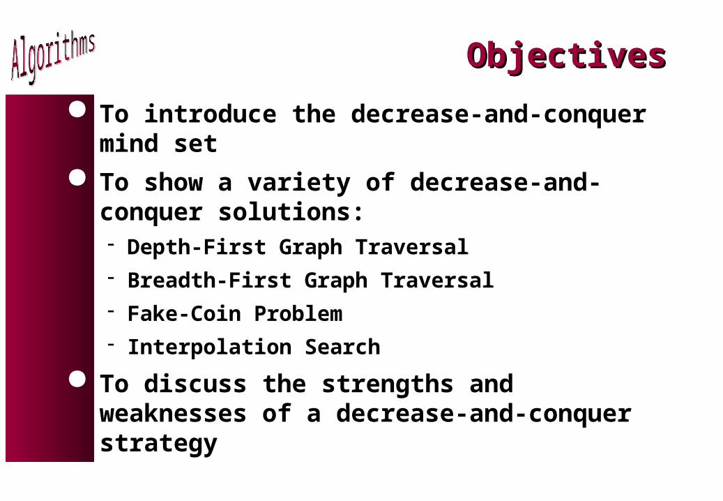
ObjectivesObjectives
To introduce the decrease-and-conquer mind set
To show a variety of decrease-and-conquer solutions: Depth-First Graph Traversal
Breadth-First Graph Traversal
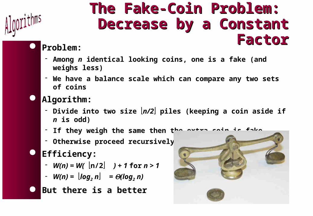
Fake-Coin Problem
Interpolation Search
To discuss the strengths and weaknesses of a decrease-and-conquer strategy
Decrease and ConquerDecrease and Conquer
1. Reduce problem instance to smaller instance of the same problem and extend solution
2. Solve smaller instance
3. Extend solution of smaller instance to obtain solution to original problem
Also called inductive or incremental
Unlike Divide-and-Conquer don’t work equally on both subproblems (e.g. Binary Search)
SUBPROBLEM OF SIZE n-1
A SOLUTION TO THEORIGINAL PROBLEM
A SOLUTION TO SUBPROBLEM
A PROBLEM OF SIZE n
Flavours of Decrease and ConquerFlavours of Decrease and Conquer
Decrease by a constant (usually 1): instance is reduced by the same constant on each iteration Insertion sort Graph Searching: DFS, BFS Topological sorting Generating combinatorials
Decrease by a constant factor (usually 2): instance is reduced by same multiple on each iteration Binary search Fake-coin problem
Variable-size decrease: size reduction pattern varies from one iteration to the next Euclid’s algorithm Interpolation Search
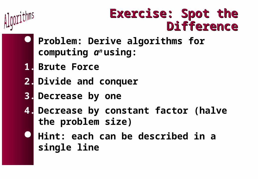
Exercise: Spot the DifferenceExercise: Spot the Difference
Problem: Derive algorithms for computing an
using:
1. Brute Force
2. Divide and conquer
3. Decrease by one
4. Decrease by constant factor (halve the problem size)
Hint: each can be described in a single line
Graph TraversalGraph Traversal
Many problems require processing all graph vertices in a systematic fashion
Data Structures Reminder:
Graph traversal strategies: Depth-first search (traversal for the Brave) Breadth-first search (traversal for the Cautious)
a b
c d
a b c d
a 0 1 1 1
b 1 0 0 1
c 1 0 0 1
d 1 1 1 0
a
b
c
d
a
b c d
d
a da b c
Depth-First SearchDepth-First Search
Explore graph always moving away from last visited vertex
Similar to preorder tree traversal
DFS(G): G = (V, E)
count 0
mark each vertex as 0
FOR each vertex v V DO
IF v is marked as 0
dfs(v)
dfs(v):
count count + 1
mark v with count
FOR each vertex w adjacent to v DO
IF w is marked as 0
dfs(w)
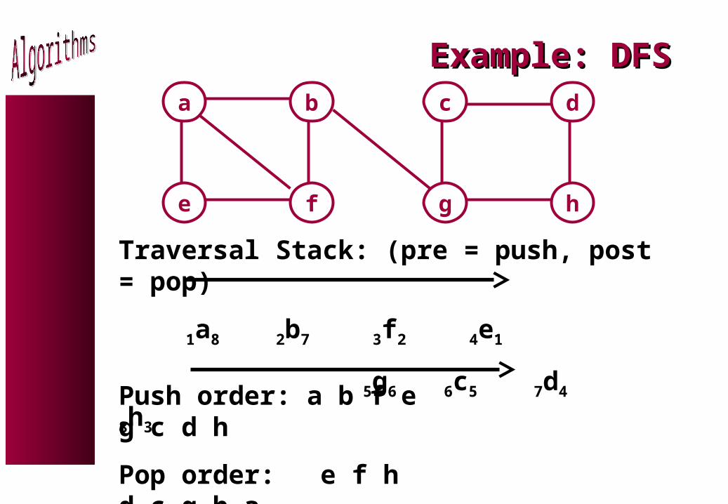
Example: DFSExample: DFSa b
e f
c d
g h
Traversal Stack: (pre = push, post = pop)
1a8 2b7 3f2 4e1
5g6 6c5 7d4 8h3
Push order: a b f e g c d h
Pop order: e f h d c g b a
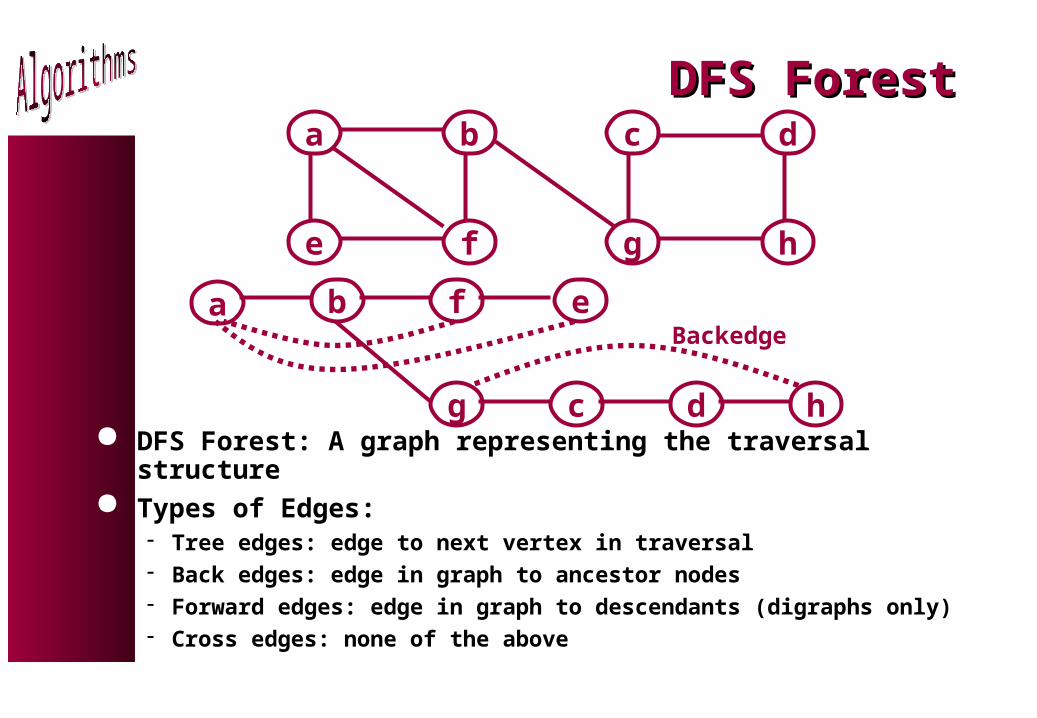
DFS ForestDFS Forest
DFS Forest: A graph representing the traversal structure Types of Edges:
Tree edges: edge to next vertex in traversal Back edges: edge in graph to ancestor nodes Forward edges: edge in graph to descendants (digraphs only) Cross edges: none of the above
a b
e f
c d
g h
a b ef
c dg h
Backedge
Notes on Depth-First SearchNotes on Depth-First Search
Implementable with different graph structures: Adjacency matrices: (V2)
Adjacency linked lists: (V+E)
Yields two orderings: preorder: as vertices are 1st encountered (pushed)