Chapter 2Theory of Anomalous Magnetic DipoleMoments of the Electron
Masashi Hayakawa
Abstract The anomalous magnetic dipole moment of the electron, the so-calledelectron g − 2, provides us with a high-precision test of quantum electrodynamics(QED), which is the relativistic and quantum-mechanical generalization of electro-magnetism, and helps to determine the value of the fine structure constant α, one ofthe fundamental physical constants. This article intends to give a pedagogical intro-duction to the theory of g − 2, in particular, the computation of high-order quantumelectrodynamics in g − 2.
2.1 Introduction
A single electron is known to becomemagnetized due to its intrinsic charge and spin.Its magnetic dipole moment is given by
µ = −gee�
2mecs , (2.1)
whereme and s denote the mass and spin of an electron, respectively. The constant ge
represents the strength of themagnetic dipole moment in units of the Bohr magneton,and is called the g-factor of the electron.
At the zeroth order of perturbation, QED predicts that gψ is equal to 2 for everymassive particle ψ with spin 1
2 . The quantum correction in general shifts gψ from2, depending on the particle species ψ . It is thus convenient to focus on this shift,called the ‘anomalous magnetic dipole moment’, by introducing a symbol
M. Hayakawa (B)
Department of Physics, Nagoya University, 464-8602 Nagoya, Japane-mail: [email protected]
We shall call this quantity g − 2 of ψ hereafter.An important point to notice is the fact that the electron g−2, ae, can be measured
very accurately. The most accurately measured value of the electron g − 2
ae(HV08) = 1 159 652 180.73 (28) × 10−12 , (2.3)
where the numerals in the parenthesis represent the uncertainty in the final fewdigits, was obtained by theHarvard group using a Penning trapwith cylindrical cavity[1, 2]. The uncertainty (2.3) is smaller than the one obtained byWashington universitygroup in 1987 [3] by a factor 15. See the previous chapter by Gabrielse et al. fora detailed explanation about how such a large reduction of uncertainty has beenachieved.
Even if g−2 is measured very accurately, onemaywonder what physical implica-tion it possesses.Worthy of note is the fact that aψ is a predictable quantity in so far asthe theory is renormalizable in the framework of quantum field theory. (Section 2.2introduces the notion and the foundation of the quantum field theory for the readersnot specialized in particle physics.) We are thus inclined to question the validity ofa renormalizable model of elementary particles by asking the compatibility of itstheoretical prediction aψ(th) with the experimentally measured value aψ(exp).
The standard model of elementary particles has endured most of tests for theseforty years. It is a renormalizable theory and thus gives a prediction to g −2, referredhereafter as aψ(SM). The measured value aψ(exp) in the experiment may containthe potential contribution aψ(new) from the structures which are not built in thestandard model
aψ(exp) = aψ(SM) + aψ(new) . (2.4)
One’s actual interest is the existence of such new structures, and its effect on g − 2of ψ . Nevertheless, in order to explore its existence through the study of g − 2, it isindispensable to compute all relevant dynamics of the standard model contributingto aψ(SM), and ask if the difference, aψ(exp)−aψ(SM), is not zero within availableprecision.
As is elucidated in full detail in Table 2.1, all the contributions relevant to aμ(SM)
can be classified unambiguously and exclusively into three components;
Table 2.1 Classification into QED, QCD and weak contributions
Type Definition
aψ(QED) QED with charged leptonsa onlyaψ(QCD) (QED + QCD) \(QED with charged leptons only)b
aψ(weak) All othersa All known charged leptons are electron (e), muon (μ) and tau-lepton (τ )b A\B for the sets A and B denotes the intersection of A and the complement of B
2 Theory of Anomalous Magnetic Dipole Moments of the Electron 43
Fig. 2.1 The Feynmandiagram giving the lowest-order (second-order) con-tribution to the anomalousmagnetic moment of thelepton
aψ(SM) = aψ(QED) + aψ(QCD) + aψ(weak) . (2.5)
The QED contribution aψ(QED) is the most dominant among these. For instance,the contribution of the leading order, O(α),1 of perturbation is induced from theFeynman diagram shown in Fig. 2.1 [4]. (Brief explanation on Feynman diagramscan be found in Sect. 2.2.1.) Figure 2.1, where time flows in the right direction,describes a process in which a single virtual photon is emitted before the leptonψ couples to the external magnetic field, and is absorbed after that. The theory ofaψ(QED) is our primary concern in this article.
In Eq. (2.5), aψ(QCD) represents the contribution from QCD. QCD is the gaugetheory of strong interactionwhich binds quarks to formnucleons. Such a contributionarises because every quark has a non-zero electric charge. Figure 2.2 illustrates theQCD contribution to the g − 2. There, a virtual photon turns into a pair of quark andanti-quark, which receive dynamics of strong interaction and then annihilate into avirtual photon again. aψ(QCD) requires evaluation of non-perturbative dynamics ofQCDin somemanner, and is thus themost difficult to compute.Theweak contributionaψ(weak) comes from the Feynman diagrams, each of which contains at least one
Fig. 2.2 The O(α2) QCDcontribution to the anomalousmagnetic moment of the lep-ton, called the ‘leading-orderhadronic vacuum polarizationcontribution’, aψ(had.v.p.).The blob part denotes therenormalized correlation func-tion 〈0| T jemμ (x) jemν (y) |0〉 ofthe hadronic electromagneticcurrent jemμ in QCD + QED
1 The fine structure constant α is given in terms of the elementary charge e and vacuum permittivityε0 by
α = e2
4πε0�c. (2.6)
44 M. Hayakawa
virtual W boson, Z boson or Higgs particle. Section 2.3 explains the basic materialson these non-QED contributions.
Importantly, the sizes of individual contributions on the right hand side of Eq. (2.5)depend sensitively on the mass mψ of the species ψ . For larger mψ , aψ(QCD) andaψ(weak) are enhanced relative to aψ(QED). Since the muon is heavier than theelectron by a factor of about 200, aμ(QCD), for instance, is about 40,000 timeslarger than ae(QCD). Likewise, aμ(new), the contribution from the as-yet-unknownstructures, may also be much larger than ae(new). This motivates us to study themuon g − 2 in a serious manner on both sides of experiment and theory, although itis not discussed fully here.
As advocated above, this article intends to give a pedagogical introduction to theQED contribution, ae(QED), to the electron g − 2. Section 2.2 provides the genericreaders with the introduction of QED, quantum field theory, perturbation theory,and the anomalous magnetic dipole moment in terms of the field theory. Section 2.3describes the current status of the non-QED contributions. The basic materials of thenumerical approach to the computation of high-order QED contributions is explainedin Sect. 2.4. Section 2.5 summarizes the latest result for ae(QED).
2.2 QED and Anomalous Magnetic Dipole Moment
2.2.1 Perturbation Theory of QED
Throughout this article, we work with the natural unit in which the speed of light cand the reduced Planck constant � are set to unity, andwith the signature of themetricημν = diag (1, −1, −1, −1) = ημν with respect to the coordinates xμ = (ct, x) infour-dimensional Minkowski space. Einstein convention is employed; the sum over0, 1, 2, 3 is assumed if the same Greek letter appears twice as a subscript and asuperscript in a single term, e.g.,
Tμν uν ≡3∑
ν=0
Tμν uν . (2.7)
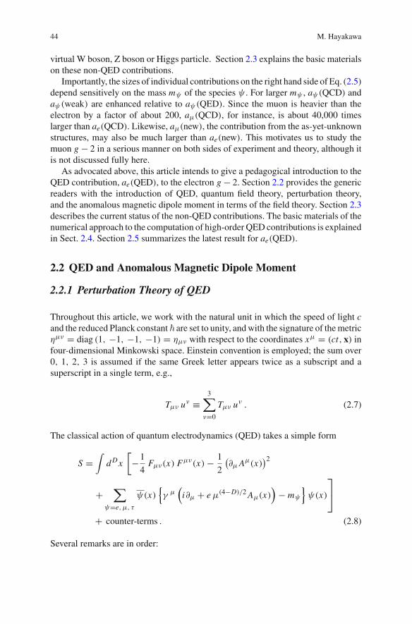
The classical action of quantum electrodynamics (QED) takes a simple form
S =∫
d Dx
[−1
4Fμν(x) Fμν(x) − 1
2
(∂μ Aμ(x)
)2
+∑
ψ=e, μ, τ
ψ(x){γ μ(
i∂μ + e μ(4−D)/2Aμ(x))
− mψ
}ψ(x)
⎤
⎦
+ counter-terms . (2.8)
Several remarks are in order:
2 Theory of Anomalous Magnetic Dipole Moments of the Electron 45
1. Thefield strength Fμν(x) is given in terms of the four-dimensional vector potentialAμ(x) = (φ(x), A(x)), Aμ(x) ≡ ημν Aν(x) by
Fμν = ∂μ Aν − ∂ν Aμ = −Fνμ . (2.9)
Fμν(x) packs the electric field E(x) and the magnetic field B(x) in the followingmanner
E j (x) = F0 j (x) ( j = 1, 2, 3) , B1(x) = F23(x) and cyclic permutation.(2.10)
Through this correspondence, the term bilinear with respect to Fμν(x) in Eq. (2.8)turns out to be the familiar action for the electric and magnetic field
∫d Dx
(−1
4Fμν(x) Fμν(x)
)=∫
d Dx1
2
(|E(x)|2 − |B(x)|2
). (2.11)
2. The quantum field theory gives a “unified description of matter and force” interms of quantum fields. Based on the particle-wave duality in quantum theory,we associate a variable called ‘quantum field’ to every species from the point ofview of a wave. In classical electromagnetism, every component of the vectorpotential Aμ(x) takes its value in a real number at every space-time point x .After quantization, Aμ(x) becomes a collection of Hermitian operators labelledby (x, μ), and plays the role of creating and annihilating photons, quanta of light.To describe creation and annihilation of one lepton speciesψ and its anti-particle,a four-component Dirac field
(ψα(x), ψα(x)
)(α = 1, 2, 3, 4) is introduced and
promoted to the fields which takes its values in the operators. Gamma matricesγ μ (μ = 0, 1, 2, 3) are a set of 4 × 4 matrices satisfying the Clifford algebracorresponding to the signature ημν
γ μγ ν + γ νγ μ = 2ημνI4. (2.12)
3. In Eq. (2.8), the sum is taken over only three leptons, i.e., electron e, muon μ andtau-lepton τ , to focus on the QED contribution in aψ hereafter.
4. In quantum field theory, the amplitude corresponding to a Feynman diagramin general suffers the divergence due to short-distance singularity (ultra-violet(UV) divergence) and the divergence due to long-distance singularity (infrared(IR) divergence). To regularize these singularities, dimensional regularization isemployed, which renders the amplitude well-defined by putting the space-timedimension D away from 0 and all positive integers on the complex plane [5].A parameter μ with dimension of mass is introduced to keep e dimensionless.
46 M. Hayakawa
5. The second term in (2.8) is the gauge-fixing term in Feynman gauge.6. The counter-terms in Eq. (2.8) are treated as the interactions which absorb the
divergences emerging from the quantum-mechanical dynamics of the terms inthe first integral of Eq. (2.8), Their details will be described in Sect. 2.2.4.
2.2.2 Feynman Diagrams and Feynman Rule
Feynman diagrams provide us with a convenient tool to figure all electromagneticprocesses relevant to the quantity and the perturbative order of one’s interest. Inperturbation theory, every term bilinear in fields in the action2 represents the propa-gation of a particle (or an antiparticle), while every term trilinear or higher in fieldsrepresents the interaction between three or more particles. A Feynman diagram isa graph describing how virtual photons, leptons and anti-leptons are created andannihilated in the following way;
1. an undirected wavy line corresponds to the propagation of a free photon,2. a directed line3 corresponds to the propagation of a free lepton,3. a vertex represents the fundamental interaction between lepton and photon.
The Feynman rule [6] derived from the action (2.8) associates the following quan-tities to a wave line, a directed line and a vertex, respectively where p/ ≡ pμγ μ.
In the graph on the left hand side of the latter equation all lines just guide theeyes, and the quantity on the right hand side is associated with the vertex alone. ‘iεwith ε > 0’ plays the role to specify the boundary condition of Green functions; ε
is brought to zero after rotating the zeroth component p0 of four-momentum to theEuclidean one p4; p0 → ip4.
The amplitude corresponding to a Feynman diagram is obtained by
2 This applies to the terms except for the counter-terms. All the counter-terms, including bilinearterms, are treated as interactions. See Sect. 2.2.4.3 There are actually three types of directed line depending on the species of leptons. See thecorresponding Feynman rule (second of the above).
2 Theory of Anomalous Magnetic Dipole Moments of the Electron 47
(a) assigning the quantities to the lines or vertices involved in a Feynman diagram,(b) imposing energy-momentum conservation at every vertex,(c) integrating n number of independent loop momenta kr (r = 1, . . . , n) with
n∏
r=1
∫d Dkr
(2π)D. (2.13)
For instance, a Feynman diagram in Fig. 2.1 gives the amplitude A μαβ(p, q)
i e μ(4−D)/2A μαβ(p, q) =
∫d Dk
(2π)D
[i e μ(4−D)/2 γλ
i
k/ + p/ + q//2 − 1
×i e μ(4−D)/2 γ μ i
k/ + p/ − q//2 − 1i e μ(4−D)/2 γ λ
]
αβ
×−i
k2. (2.14)
Here, q is the four-momentum of the incoming photon, p∓q/2 are the four-momentaof incoming and outgoing external leptons, respectively. The loopmomentum is takento be the momentum k carried by the virtual photon. Since g − 2 is a dimensionlessquantity, it is convenient to express all dimensionful quantities in units of the massof the external lepton, parametrizing the effect of creation and annihilation of virtualleptons by lepton mass ratios, which appears at the fourth and higher orders. Forthis reason, the masses in Eq. (2.14) are set to 1. The amplitude (2.14) containsthe overall ultra-violet-divergent monopole contribution as well. The contributionto the anomalousmagnetic dipolemoment from Fig. 2.1 will be obtained by applyingthe magnetic projection to be discussed in Sect. 2.2.3, to the amplitude (2.14).
For the sake of later reference, the standard technique in quantum field theory tocalculate (2.14) is explained here. We can show the identity
1
ABC= 1
2
∫ 1
0dz1
∫ 1
0dz2
∫ 1
0dza δ (1 − (z1 + z2 + za))
1
(za A + z1B + z2C)3.
(2.15)Applying Eq. (2.15) to the integrand of Eq. (2.14)with A = k2, B= (k+p+q/2)2−1and C = (k + p − q/2)2 − 1, and exchanging the order of integration, the integralover the loop momentum k can be easily evaluated.4 The resulting integral is the onewith respect to Feynman parameters za , z1 and z2.
4 One can consult with the content of Sect. 2.4.2 on this point.
48 M. Hayakawa
2.2.3 Anomalous Magnetic Dipole Moment
In this section,we see how the contribution to the anomalousmagnetic dipolemomentcan be extracted from the amplitude in the context of quantum field theory.
Let Γμ
B, αβ(p, q) be the unrenormalized vertex function, i.e., the contribution of
the one-particle irreducible5 Feynman diagrams to the Green function
(2.16)where jμem(x) is the electromagnetic current, pF = p + q
2 and pI = p − p2 . The
renormalized vertex function Γμαβ(p, q) is given in terms of the wave function renor-
malization constant Zψ of the external lepton by
Γμαβ(p, q) = Zψ Γ
μB, αβ(p, q) . (2.17)
The invariance of QED under Lorentz-, charge conjugation-(C) and parity (P)transformations as well as the gauge symmetry implies that the renormalized vertexfunction with the external leptons put on their mass shells, but with the externalphoton kept off-shell, consists of two form factors F1(q2), F2(q2)6;
Γμαβ(p, q)
∣∣∣p2F =m2
ψ=p2I= F1(q
2)γ μ + F2(q2)
1
2mψ
iσμνqν , (2.18)
where
σμν ≡ i
2
[γ μ, γ ν
]. (2.19)
The on-shell renormalization condition imposes F1(q2 = 0) = 1 to the electricform factor. The magnetic form factor F2(q2) is the quantity predictable in therenormalizable theory. The anomalous magnetic dipole moment is actually identifiedwith F2(q2 = 0)
aψ = F2(0) . (2.20)
It is an easy exercise to see that aψ is obtained by applying the magnetic projectionto Γ
μαβ(p, q);
5 A Feynman diagram is called ‘one-particle irreducible’ if and only if it cannot be divided intotwo non-trivial connected subdiagrams when any one of the internal lines is cut off.6 C and P symmetries are violated in the weak and Yukawa interactions in the standard model, andthus additional form factors are actually induced. However, the classification in Table 2.1 insuresthat QED and QCD contributions, which respect C and P symmetry, consist of two form factors asin Eq. (2.18).
2 Theory of Anomalous Magnetic Dipole Moments of the Electron 49
aψ = limq2→0
mψ
4q2(
p2)2 tr
[{mψ p2γ μ −
(m2
ψ + q2
2
)pμ
}
×(
p/ + q/
2+ mψ
)Γμ(p, q)
(p/ − q/
2+ mψ
)], (2.21)
with the on-shell conditions p · q = 0 and p2 + q2/4 = m2ψ for the external leptons.
The second-order contribution toaψ is obtained by applying (2.21) toΓ μ(p, q) =A μ(p, q) in Eq. (2.14) as [4]
aψ
∣∣1-loop = α
2π. (2.22)
2.2.4 Renormalization and Counter-Terms
In perturbation theory of quantum field theory, the notion of counter-terms providesa systematic and practical way to calculate the renormalized amplitude.
The “counter-terms” in (2.8) take the form
Sc.t =∫
d Dx
[−1
4δZ A Fμν Fμν
+∑
ψ=e, μ, τ
{δZψ ψγ μi∂μψ − δZ M, ψ mψψψ
+ δZV, ψ eμ(4−D)/2ψγ μ Aμψ}]
. (2.23)
and are adjusted to absorb UV divergence. The constants appearing above, δZ A,δZψ , δZ M, ψ and δZV, ψ are related to the wave function renormalization con-stants Z A, Zψ ,multiplicativemass renormalization constant Zm, ψ
7 and the couplingrenormalization constant Ze through
δZ A = Z A − 1 , δZψ = Zψ − 1 ,
δZ M, ψ = Zψ Zm, ψ − 1 , δZV, ψ = Ze Zψ Z1/2A − 1 . (2.24)
Perturbatively, the coefficients of counter-terms are expanded in a power series ofα/π ,
7 Here we assume that the regularization preserves the non-anomalous chiral symmetry, so that nolinear additive UV divergence arises in the two-point functions of leptons.
50 M. Hayakawa
δZ A =∞∑
n=1
δ(n)Z A
(α
π
)n, δZψ =
∞∑
n=1
δ(n)Zψ
(α
π
)n,
δZ M, ψ =∞∑
n=1
δ(n)Z M, ψ
(α
π
)n, δZV, ψ =
∞∑
n=1
δ(n)ZV, ψ
(α
π
)n. (2.25)
These counter-terms generate the interaction vertices of various orders of perturba-tion theory. In particular, the renormalization ofwave function ormass corresponds toa vertex from which only two lines emanate. The lower-order counter-terms togetherwith QED interaction generate the Feynman diagrams and the subtraction termswhich cancel ultra-violet divergences contained in subdiagrams. In the end, the sumof all those Feynman diagrams can have only overall UV divergences that should becancelled by the nth-order coefficients, δ(n)Z A, etc. Their precise values are deter-mined from the demand that the renormalized vertex functions, Π(q2), �αβ(p) and�μ(p, q), defined by
∫d Dx eiq·x 〈0| Aμ(x)Aν(0) |0〉 = −iημν
q2{1 − Π(q2)
} ,
∫d Dx eip·x 〈0| ψα(x)ψβ(0) |0〉 =
[i
p/ − m − �(p)
]
αβ
,
Γμαβ(p, q) = γ
μαβ + �
μαβ(p, q) , (2.26)
satisfy certain renormalization conditions. The gauge symmetry guarantees that Ze
is independent of ψ . In this way, the counter-terms are determined iteratively inperturbation theory of QED.
2.2.5 Classification of Perturbative Dynamics
The quantum electrodynamics in the lepton g − 2, aψ(QED), are expected to be
obtained by computing the coefficients a(2n)ψ in the perturbative series
aψ(QED) =∞∑
n=1
a(2n)ψ
(α
π
)n, (2.27)
up to the order N determined from the requirement of experimental accuracy and ourtheoretical interest. In what follows, the nth term in Eq. (2.27) is called ‘n-loop term’or the ‘2nth-order term’, as it is O(α n) ∼ O(e 2n). The comparison of Eq. (2.22)with (2.27) yields the leading-order coefficient a(2)
ψ as
a(2)ψ = 1
2≡ A(2)
1 . (2.28)
2 Theory of Anomalous Magnetic Dipole Moments of the Electron 51
Before starting any calculations, themost dominant contribution should be identified.To do so in our context, we decompose the contributions into four types accordingto the dependence on lepton mass ratios (Recall the discussion below Eq. (2.14.));
a(2n)e = A(2n)
1 + A(2n)2
(me
mμ
)+ A(2n)
2
(me
mτ
)+ A(2n)
3
(me
mμ
,me
mτ
). (2.29)
Here, the subscript j attached to A(2n)j denotes the number of leptons involved in its
calculation. A(2n)1 is the contribution that should be computed in QED with electron
only. It is a pure number and called ‘mass-independent term’, and thus universally
contributes to g − 2 of all leptons ψ . A(2)1 is given by Eq. (2.28). A(2n)
2
(me
mμ
)is the
contribution to the electron g −2 from all Feynman diagrams with at least one muon
loop butwith no tau-lepton loop. A(2n)2
(me
mτ
)is similarly defined. A(2n)
3
(me
mμ
,me
mτ
)
is the contribution of all Feynman diagrams with both muon loop(s) and tau-leptonloop(s). A(2n)
2 appears at first at the fourth order. A(2n)3 appears at first at the sixth
order.Muon and tau-lepton are both much heavier than the electron. Thus, for the elec-
tron g − 2, their virtual effects are suppressed compared to the dynamics of QEDwith electron only. Therefore, A(2n)
1 is the most dominant at every order 2n in theelectron g − 2.
It would be instructive to compare such a perturbative feature of QED in theelectron g − 2 with that in the muon g − 2. In the similar manner as in (2.29), eachcoefficient a(2n)
μ in the perturbative expansion of aμ(QED) can be decomposed intofour types of terms;
a(2n)μ = A(2n)
1 + A(2n)2
(mμ
me
)+ A(2n)
2
(mμ
mτ
)+ A(2n)
3
(mμ
me,
mμ
mτ
). (2.30)
The meaning of each term would now be obvious from the dependence on lepton
mass ratio(s). Since the electron is lighter than the muon, A(2n)2
(mμ
me
)dominates
a(2n)μ for 2n ≥ 6.
2.3 Non-QED Contribution to g − 2
The standard model contribution was decomposed into three parts as in Eq. (2.5).Table 2.2 summarizes the results for the non-QED contribution to the electron g − 2obtained thus far. In that table, the last one is the weak contribution, and the othersare the QCD contributions relevant to the precision of our interest. Table 2.2 also
52 M. Hayakawa
Fig. 2.3 Examples ofthe next-to-leading-order(O(α3)) hadronic vacuumpolarization contribution,aψ(NLO had.v.p.), to theanomalous magnetic dipolemoment
shows that they are only small part of ae, but can no longer be neglected compared tothe current experimental accuracy (2.3). Below we focus on the QCD contribution.
The QCD contributions relevant to the electron g − 2 in view of the experimen-tal accuracy are represented by the diagrams shown in Figs. 2.2, 2.3 and 2.4, andae(QCD) is given by their sum
Here, O(α2)-hadronic vacuum polarization contribution, ae(had.v.p.), correspondsto the diagram in Fig. 2.2. Note that it also includes the O(α3)-terms caused by a
2 Theory of Anomalous Magnetic Dipole Moments of the Electron 53
single virtual photon exchange between quarks in the blob part. The QED correctionto a photon line, lepton line or leptonic vertex in Fig. 2.2 gives rise to the next-to-leading-order (NLO) hadronic vacuum polarization contribution, ae(NLO had.v.p.).Figure 2.3 illustrates a Feynman diagram contributing to ae(NLO had.v.p.). Lastly,the hadronic light-by-light scattering contribution shown in Fig. 2.4, ae(had.l-l), isalso the order ofα3, and is induced through the elastic scattering between two photonscaused by QCD.
Since the strongly coupled dynamics at low energy�1 GeV is the most importantto the electron g−2, perturbation theory ofQCDcannot account for the bulk contribu-tion to the lepton g−2. In general, we must rely on some numerical means to capturethe non-perturbative dynamics of QCD. For the hadronic vacuum polarization typecontributions, i.e., aψ(had.v.p.) and aψ(NLO had.v.p.), we can circumvent directcomputation of non-perturbative QCD dynamics as follows. The dispersive expres-sion for the vacuum polarization function and the optical theorem, which followsfrom the unitary of S matrix, enables to express aψ(had.v.p.) as the convolution ofR ratio R̂(s), where
√s = 2Ecm for the electron energy Ecm in the center of mass
frame of the electron and positron beams, and a calculable function K (s)
aψ(had.v.p.) =( α
3π
)2 ∫ ∞
E2th
ds
s
m2ψ
sR̂(s) K (s) , (2.32)
with Eth = mπ0 . The function K (s) increases from 0.4 at Eth monotonically andapproaches to 1 for s → ∞. (The explicit expression of K (s) is available, e.g. in [7].)To take the O(α) QED correction to the blob part in Fig. 2.2 into account, we focuson the the cross section σh(s) in the unpolarized e+e− collision with the hadrons orhadrons +γ as the final states, but with no initial state photon radiation. Note thatthe R ratio R̂(s) required in Eq. (2.32) is not the experimentally accessible quantityσh(s), but σ̂h(s) which is obtained from σh(s) by removing O(α) correction to thepart e+e− → γ ∗
R̂(s) = σ̂h(s)
4πα2
3s
. (2.33)
The additional QED correction residing in σh(s) compared to σ̂h(s) is exactly thecharge renormalization. Therefore, these two quantities are related as
σ̂h(s) =(
α
α(s)
)2
σh(s) , (2.34)
where, for the relevant order of α, σ(e+e− → γ ∗ → hadrons) only suffices forthe QCD effect in the running gauge coupling constant α(s). aψ(NLO had.v.p.) canalso be obtained with use of σ(e+e− → γ ∗ → hadrons) and the different functionfor K (s).
54 M. Hayakawa
Table 2.2 Summary of non-QED contribution to the electron g − 2
The first three are QCD contributions. ae(weak) is estimated by scaling aμ(weak)with the electron-muon mass ratio took into account
Practically, an inclusive cross section is impossible to directly measure; it is actu-ally obtained by summing up all relevant exclusive cross sections. Experimentalpapers have reported their results for the individual cross section with or withoutradiative corrections, and thus careful treatment is necessary to gather and compilevarious data [8].
In contrast to the vacuum-polarization-type contribution, the hadronic light-by-light scattering contribution has not been successfully expressed in terms of someexperimentally accessible quantities, and thus it requires explicit theoretical compu-tation of non-perturbative QCD dynamics. The computation of this quantity is oneof the remained subjects of the lepton g − 2, in particular, the muon g − 2. Thus far,it has been mostly evaluated according to the low-energy effective theory of QCDand/or hadronic models. ae(had.l-l) in Table 2.2 was also obtained in this manner[10]. Even though its order in Table 2.2 is found to be much smaller than the one ofour interest, it should be calculated by some other method.
2.4 Numerical Approach to Perturbative QED Calculation
The perturbative coefficients a(2n)ψ have been known exactly or as an expansion in
power series ofmass ratios forn = 1, 2, 3. (SeeSect. 2.5 for the literature concerningwith the lower-order coefficients.) The eighth-order coefficient a(8)
ψ and the tenth-
order coefficient a(10)ψ [15–24], however, have been evaluated only by numerical
means. Here, a succinct explanation is given for a particular method adopted tocompute a(8)
ψ and a(10)ψ . The reader who would like to know full details on the
parametric integral formalism, in particular on the ways of construction of ultra-violet and infrared subtraction terms can consult with the review article [25] or theoriginal references [26–29].
2.4.1 Classification of Feynman Diagrams
Here we see the scheme of classification of Feynman diagrams employed in a seriesof works [15–24].
2 Theory of Anomalous Magnetic Dipole Moments of the Electron 55
Fig. 2.5 A self-energy-like Feynman diagram (4a) corresponding to three vertex-type diagramsgiving the fourth-order contribution to the anomalous magnetic moment of the lepton
Fig. 2.6 The vertex diagrams at the fourth order related to a self-energy-like diagram in Fig. 2.5via Ward-Takahashi identity (2.35)
We start with introducing the notion of self-energy-like (Feynman) diagram.A self-energy-like diagram is a diagram obtained from a vertex diagram by remov-ing the external vertex. Note that the contribution to the self-energy function from aself-energy-like diagram may vanish identically. Such an example is the sixth-orderlight-by-light scattering diagram, where the external vertex lies on the virtual leptonloop. Note also that two different vertex diagrams are possibly reduced to the sameself-energy-diagram if the external vertices are removed.
The reasonwhywe focus on self-energy-like diagrams in place of vertex diagramsis based on the following important but unfamiliar fact; the Ward-Takahashi (WT)identity, which results from the gauge invariance of the system, holds between thecontribution to the self-energy functionΣ(p) froma single self-energy-like Feynmandiagram G and the contribution to the vertex function Λμ(p, q) from a set BG ofvertex diagrams which can be obtained by inserting a single QED vertex into oneof the lepton lines on the open path connected to the initial and final leptons, or theloop with odd number of internal vertices in all possible ways;
∑
V ∈BG
qν�νV (p, q) = −�G
(p + q
2
)+ �G
(p − q
2
). (2.35)
For instance, to the self-energy function�G froma single self-energy-like diagramG in Fig. 2.5, the sum of contributions to the vertex functions from three diagramsin Fig. 2.6 are related through Eq. (2.35).
By differentiating both sides of Eq. (2.35) with respect to the incoming photonmomentum qμ, and taking the limit q → 0, we find
∑
V ∈BG
�μ
V (p, q 0) ∑
V ∈BG
{−qν
[∂�ν
V (p, q)
∂qμ
]
q=0
}− ∂�G (p)
∂pμ
. (2.36)
56 M. Hayakawa
I(a) I(b) I(c) I(d) I(e)
I(f) I(g) I(h) I(i) I(j)
II(a) II(b) II(c) II(d) II(e)
II(f) III(a) III(b) III(c) IV
V VI(a) VI(b) VI(c) VI(d) VI(e)
VI(f) VI(g) VI(h) VI(i) VI(j) VI(k)
Fig. 2.7 Gauge-invariant subsets of self-energy-like diagrams at the tenth order
Via this identity, it is possible to obtain the expression of the sum MG of the bareamplitudes of g − 2 induced from the vertex diagrams in BG which are related toa single self-energy-diagram G simultaneously, once we find the expression of theintegrand for the bare Feynman amplitude of �G (p) in the momentum space.
Moreover, all the vertex diagrams belonging toBG have similar ultra-violet (UV)and infrared (IR) divergent structures, as we will see this point explicitly within theparametric integral formalism in Sect. 2.4.3. Since the number of self-energy-likediagrams ismuch smaller than that of the vertex diagrams by the factor 1/(2n−1), wefirst categorize the vertex diagrams at the order of our interest into the sets representedby the corresponding self-energy-like diagrams.We next classify the self-energy-likediagrams into the minimal gauge-invariant subsets. Note that a gauge-invariant setmeans the set of diagrams whose sum of contributions is independent of the choiceof gauge fixing condition. The minimal gauge-invariant subsets can be immediatelyidentified if one’s attention is paid to the types and the number of lepton loopsinvolved. This point can be seen in Fig. 2.7, which lists up all the gauge-invariantsubsets for the self-energy-like diagrams at the tenth order [15, 28].
2 Theory of Anomalous Magnetic Dipole Moments of the Electron 57
2.4.2 Parametric Representation of Feynman Diagrams
As introduced inSect. 2.2.1, the amplitude can be expressed as an integral of Feynmanparameters. Here, we overview a way to write down the bare amplitude in terms ofbuilding blocks which will turn out to help to construct the terms cancelling theultra-violet and infrared divergences on the Feynman parameter space.
For that purpose, we return to Eq. (2.14), and overview the standard calculationalmethod of the Feynman amplitude. The numerator of the integrand of Eq. (2.14)involves
{k/ + p/ + q/
2+ 1
}⊗{
k/ + p/ − q/
2+ 1
}, (2.37)
which can be written in terms of k = l − z1(
p + q2
) − z2(
p − q2
)with new loop
momentum l as
f
{l/ + (1 − z1)
(p/ + q/
2
)− z2
(p/ + q/
2
)+ 1
}
⊗{
l/ − z1
(p/ + q/
2
)+ (1 − z2)
(p/ − q/
2
)+ 1
}. (2.38)
Now that the denominator is an even function of l, the terms with odd number of lin the numerator all vanish upon loop integration. Thus, the integral consists of twotypes
∫d Dl
(2π)D
lμlν{l2 − C(z1, z2) + iε
}3 ,
∫d Dl
(2π)D
1{l2 − C(z1, z2) + iε
}3 , (2.39)
which can be performed easily.Even at higher order of perturbation, themanipulation towrite down the amplitude
as an integral on Feynman space is essentially the same. In practice, however, it needssuch devises that realize
(1) construction of the bare amplitude can be systematically done,(2) construction of the terms to numerically subtract ultra-violet divergence and
infrared divergence can be done systematically.
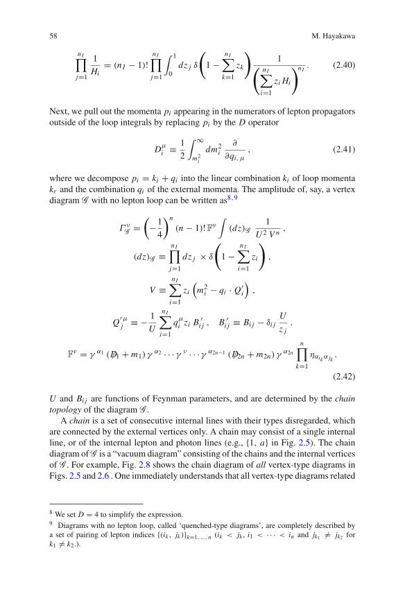
The parametric integral formalism provides a method to calculate the perturbativecoefficients numerically with the properties (1) and (2). There, the numerical cal-culation is done on the Feynman parameter space. The loop momenta {kr }r=1, ··· , n(n is the total number of loops.) must thus be carried out manually. To do so, we firstconvert nI number of the denominators of propagators (nI denotes the number ofinternal lines in the diagram) to a single denominator through the formula
58 M. Hayakawa
nI∏
j=1
1
Hi= (nI − 1)!
nI∏
j=1
∫ 1
0dz j δ
(1 −
nI∑
k=1
zk
)1
( nI∑
i=1
zi Hi
)nI. (2.40)
Next, we pull out the momenta pi appearing in the numerators of lepton propagatorsoutside of the loop integrals by replacing pi by the D operator
Dμi ≡ 1
2
∫ ∞
m2i
dm2i
∂
∂qi, μ, (2.41)
where we decompose pi = ki + qi into the linear combination ki of loop momentakr and the combination qi of the external momenta. The amplitude of, say, a vertexdiagram G with no lepton loop can be written as8,9
U and Bi j are functions of Feynman parameters, and are determined by the chaintopology of the diagram G .
A chain is a set of consecutive internal lines with their types disregarded, whichare connected by the external vertices only. A chain may consist of a single internalline, or of the internal lepton and photon lines (e.g., {1, a} in Fig. 2.5). The chaindiagram ofG is a “vacuum diagram” consisting of the chains and the internal verticesof G . For example, Fig. 2.8 shows the chain diagram of all vertex-type diagrams inFigs. 2.5 and 2.6 . One immediately understands that all vertex-type diagrams related
8 We set D = 4 to simplify the expression.9 Diagrams with no lepton loop, called ‘quenched-type diagrams’, are completely described bya set of pairing of lepton indices {(ik , jk)}k=1, ..., n (ik < jk , i1 < · · · < in and jk1 �= jk2 fork1 �= k2.).
2 Theory of Anomalous Magnetic Dipole Moments of the Electron 59
via the WT-identity to a self-energy-like diagram share a common chain diagram, ingeneral.
For a non-self-intersecting loop C , we introduce the incident matrix{ξc,C
}asso-
ciated with the chain topology of G
ξc,C =⎧⎨
⎩
1 if c ∈ C and chain c has the same direction as C−1 if c ∈ C and chain c has the direction opposite to C0 if c /∈ C
. (2.43)
Accordingly, we assign the Feynman parameter zc to the chain c as
zc =∑
j∈c
z j . (2.44)
In Figs. 2.5 and 2.8,
zc1 = z1 + za , zc2 = z2 , zc3 = z3 + zb. (2.45)
Starting with U = zc for a loop (the chain topology of the one-loop diagram), Bc1, c2and U are obtained recursively according to the following equations
Bc1, c2 =∑
C
ξc1,C ξc2,C UG /C ,
ξc,C0U =∑
c′ξc′,C0 zc′ Bc′, c . (2.46)
Here,G /C denotes the reduced diagramwhich is obtained by shrinkingC to a singlevertex in G . C0 and c in the second equation are arbitrarily chosen loop and a chainon it, respectively. Equation (2.46) shows that Bc1, c2 andU are functions of Feynmanparameters of homogeneous degrees n − 1 and n, respectively. Bi j = B ji for a pairof the internal lines i, j is equal to +Bc1, c2 for i ∈ c1, j ∈ c2 if both lines have thesame or the opposite directions as the chains, and to −Bc1, c2 otherwise.
The application of D operators contained in Fν of Eq. (2.42) will yield the terms
as in Eq. (2.39). It is straightforward to see that the manipulation of D operators isequivalent to performing all possible ways of following contraction operations :
(a) In case that Dμi and Dν
j are “contracted”, they are turned into(− 1
2 B ′i j ημν
).
(b) The uncontracted Dμi is replaced by Q′μ
i .(c) The terms obtained by k-time contraction is multiplied by
1
(n − 1) · · · (n − k)
1
U k+2 V n−k, (2.49)
in place of1
U 2V n.
The denominator of the resulting integrand is now written in terms of Bi j andQ′μ
i . A vectorial quantity Q′μi is expressed as a linear combination of the external
momenta with the scalar currents Api , Aq
i as the coefficients
Q′μi = Ap
i pμ + Aqi qμ . (2.50)
(See the explanation just below Eq. (2.14) for the meaning of p, q.) No Aqi appears
in the expression of the integrand of g − 2 amplitude. Api is given in terms of B ′
i jand U as [27]
Api = − 1
U
nI∑
j=1
η j,P z j B ′j i , (2.51)
for the path P consisting of all consecutive lepton lines connected to the externalleptonic states, and η j,P is 1 (−1) if the line j lies on P with the same (opposite)direction, and 0 otherwise.
Obviously, use of U , Bi j and Api as “building blocks” of the integrand10 reduces
the size of the expression of the integrand, compared to the one written solely in
10 The WT-summed amplitude consists of four types of terms. One is written by
C̃i j = 1
U
∑
k<l
zk zl
(B ′
ik B ′jl − B ′
il B ′jk
), (2.52)
2 Theory of Anomalous Magnetic Dipole Moments of the Electron 61
terms of {zi }, and thus reduces the computational cost significantly. Furthermore, itwill turn out that they also play the essential role in the systematic construction ofthe integrands of the terms to subtract divergence. In order to see a little bit aboutthis point, we end this section with observing when ultra-violet (UV) divergenceand infrared (IR) divergence can arise. From Eq. (2.51), it turns out that the scalarcurrents are rational functions of Feynman parameters with homogeneous degree0. Thus, V in Eq. (2.42) is a rational function with homogeneous degree 1. Hence,the terms obtained by the same number of contractions, whose integrands are allproportional to the quantity (2.49), have the same homogeneous degree. Note thatthe terms obtained by more and more number of contraction operations correspondto the ones with more and more loop momenta in the numerators of the integrands,and thus become dominated by larger and larger momenta. As seen in Eq. (2.49),contraction increases the degree ofU while it decreases that of V in the denominator.Hence, UV divergences can arise on some boundary of Feynman parameter spacewhere U → 0. Likewise, IR divergences can arise where V → 0.
2.4.3 Subtraction of UV and IR Divergences
One of the distinguishing features of the numerical method [26–29] adopted tocompute the high-order QED contribution to aψ is the numerical subtraction ofultra-violet (UV) divergences in the Feynman amplitudes. We suppose that thoseamplitudes are written in the form of the parametric integrals, as was explained inSect. 2.4.2.
The numerical subtraction of divergence can be attained only if the bare ampli-tude and all the required subtraction terms are prepared on the common Feynmanparameter space, and singularities are organized to be cancelled in a pointwise way.This way of singularity cancellation, however, requires that a single vertex-typeFeynman diagram, or some set of vertex-type Feynman diagrams sharing a commonUV structure must be dealt with separately to prepare the subtraction terms. Herewe start with observing that a collection of vertex subdiagrams associated with oneself-energy-like diagram is a reasonable example of such sets.
As already remarked, the definition of a self-energy-like diagram in Sect. 2.4.1and the definition of the chain in Sect. 2.4.2 implies that a collection of vertex-typeFeynman diagrams related to a given self-energy-like diagram shares the same chaintopology. Therefore, those vertex-type diagrams share common U and Bi j . SinceUV subdivergence appears on the boundary of Feynman parameter space where Uvanishes, these diagrams have the same UV divergent structure.
As already mentioned above, the use of the Ward-Takahashi (WT) identity (2.36)to collectively deal with a series of vertex diagrams reduces the total task neededto prepare the integrals significantly. For instance, at the tenth order, there are
(Footnote 10 continued)where the sum is taken over the lepton lines where an external photon vertex can be inserted ina self-energy-like diagram. C̃i j is actually a homogeneous polynomial of degree n. We must dealwith these C̃i j in addition to U , Bi j and Ai .
62 M. Hayakawa
6,354 quenched-type diagrams. Since nine vertex diagrams are related to each singlequenched-type self-energy-like diagram, the WT-identity (2.36) thus reduces themto 706 self-energy-like diagrams. Time reflection invariance in QED further reducesthe number of independent integrals to 389 [28].
We call the sum of the g − 2 amplitudes over the set of vertex diagrams relatedvia theWT-identity to a single self-energy-like diagram G as the WT-summed ampli-tude. The bare WT-summed amplitude, denoted by MG , in general contains infrared(IR) divergence(s). Therefore, the additional subtraction terms must be added toremove those IR divergences and to get the integral which can be carried out with asupercomputer system. Symbolically, such a finite integral takes the form
ΔMG =∫
(dz)G
⎛
⎝ f bareG (z) +∑
F
f UVF (z) +∑
G
f IRG (z)
⎞
⎠, (2.53)
Each of UV subtraction terms necessary for the muon g − 2 is in one-to-one corre-spondence with a normal forest F. A forest of a diagram G is a set of UV-divergentone-particle irreducible subdiagrams, any two of which are not overlapped with eachother.11 A forest is normal if it does not contain G as its element.
Before proceeding further, a comment on the necessity of IR subtraction is in orderhere. The sum of the on-mass-shell subtracted amplitudes over each gauge-invariantsubset {G }′, i.e.,
aψ
({G }′) =∑
{G }′
⎧⎨
⎩MG +∑
FG
FUV, on-shellFG
⎫⎬
⎭ , (2.54)
is finite. The expression on the right-hand side of Eq. (2.54) can be cast into the formrequired for the numerical subtraction
aψ
({G }′) =∑
{G }′
∫(dz)G
⎧⎨
⎩ f bareG +∑
FG
f UV, on-shellFG
⎫⎬
⎭ . (2.55)
The essence of derivation of this form can be seen in the case where G have a vertexsubdiagram S , and focus on the forest F = {S }, for simplicity. The on-mass-shellsubtraction term corresponding to {S } is given by the product
FUV, on-shell{S } = MG /S LS , (2.56)
of the vertex renormalization constant LS on mass shells and the WT-summedmagnetic moment MG /S of the reduced (self-energy-like) diagram G /S which
11 Two subdiagrams S1 and S2 are said to be overlapped if S1 ∩ S2 �= ∅, but neither S1 ⊂ S2nor S1 ⊃ S2.
2 Theory of Anomalous Magnetic Dipole Moments of the Electron 63
is obtained by shrinking S to a point-like vertex in G . The parametric integralformalism allows to express LS and MG /S as the integrals of respective sets ofFeynman parameters. Thus, their product takes the form
MG /S LS =∑
α, β
Γ (α)
∫(dz)G /S
gα [G /S ](VG /S
)α × Γ (β)
∫(dz)S
gβ [S ]
(VS )β,
(2.57)where, for instance, gα[S ] is a function with equal numbers ofUS , B ′S
i j , ASi . The
application of the formula
Γ (α)
Hα
Γ (β)
K β= Γ (α + β)
∫ 1
0ds∫ 1
0dt δ(1 − s − t)
sα−1 tβ−1
(s H + t K )α+β, (2.58)
and rescaling of the Feynman parameters will reduce Eq. (2.57) to the desired form[29]
MG /S LS =∫
(dz)G∑
α, β
Γ (α + β)gα [G /S ] gβ [S ](VG /S + VS
)α+β. (2.59)
The integrand on the right-hand side is exactly f UV, on-shell{S } in Eq. (2.55). By con-
struction, the integral in Eq. (2.55) for each G is free from UV divergence. However,it contains IR subdivergence, in general. The form (2.55) demands that cancellationof IR subdivergence be realized when the summation is taken over {G }′, not at thestage of integration. This implies that the form (2.55) may allow cancellation ofUV divergence, but never does so for IR divergence at the numerical level. This isthe reason why explicit construction of IR subtraction is necessary in the numericalapproach.
In what follows, we will see the construction of UV subtraction terms first, andthat of IR subtraction terms next.
We first concentrate on the construction of UV subtraction terms. As was stressedabove, the numerical subtraction can be attained only if the subtraction terms areprepared on the same Feynman parameter space as the bare amplitude so that the UVsingularities of the bare amplitude are cancelled in a pointwise way. As we have seenalready above, the on-mass-shell subtraction term can be cast into such a requiredform, and the maximally contracted term involved in LS in fact cancels the UVdivergence. However, the on-shell subtraction term in general brings the additionalIR divergence not present in the bare amplitude through non-maximally contractedterms. As discussed in the last paragraph in Sect. 2.4.2, lesser and lesser contractedterms tend to be dominated by the dynamics of degrees of freedom with longer andlonger wavelength.
For this reason, renormalization is processed in two steps. That is, the UV subtrac-tion terms f UVF (z) inΔMG in Eq. (2.53) are constructed according to theK operation[27], which provides the UV subtraction term free from IR subdivergence. The sec-ond step, called the residual renormalization, calculates the difference between the
64 M. Hayakawa
renormalization condition corresponding to K operation and the on-shell condition.12
This step adds the finite term R({G }′) to the sum of ΔMG over a gauge-invariant
subset {G }′a(2n)ψ
({G }′) =∑
{G }′ΔMG + R
({G }′) . (2.60)
To state the content of the K operation, we define theUV limit. For simplicity, we dealwith the forest {S } consisting of a single vertex or self-energy subdiagram S . Wesuppose that the Feynman parameters are organized to parametrize the correspondingUV singularity on the boundary zi ∼ 0 (i ∈ S ). The UV limit [A]UVS of the quantityA is defined to gather all the leading terms of ε (ε � 1) for
z j ={
O(ε) if j ∈ SO(1) otherwise
. (2.61)
Now, K operation is defined as the following manipulation on the integrand :
(1) It extracts only the maximally contracted terms.(2) Bi j , A j appearing in the numerator of the integrand and U are replaced by the
corresponding UV limits.(3) V is replaced by VS + VR , where R is the reduced diagram, and VS and VR
are written in terms of Feynman parameters and scalar currents in S and R,respectively.
(1) and (3), where V is not replaced by its UV limit, are necessary in order not tointroduce any additional IR divergences.
The most important feature of the integral obtained via K operation is the factor-ization property; the subtraction terms obtained via K operation are given by the sumof the products of the quantities associated with the subdiagrams Si of the forest{Si } and the magnetic moment of the reduced self-energy-like diagram. Again, let’sconsider a forest {S } consisting of a single UV-divergent subdiagram. If S is avertex subdiagram, R = G /S and
KS MG = LUVS MG /S , (2.62)
where LUVS denotes the maximally contracted terms of LS . If S is a self-energy
subdiagram, the result of K operation consists of two terms
KS MG = δmUVS MG /S (i∗) + BUV
S MG /{S , i} . (2.63)
In G /S (i∗), the remnant ofS is left as the mass insertion vertex (∗) on a lepton linei connecting S to the rest of G . Note that G /S (i∗) and G / {S , i} have the same
12 The masses of leptons and the electric charge can be used only for the amplitude renormalizedin the on-shell renormalization condition.
2 Theory of Anomalous Magnetic Dipole Moments of the Electron 65
chain topology so that VG /{S , i} can be used in Sect. 2.4.3. The UV-finite amplitude
MRG , which may contain IR divergence, is obtained from the forest formula with use
of K operationMR
G = MG +∑
F
∏
S ∈F(−KS ) MG , (2.64)
whose integral is organized in the same form as in Eq. (2.54).Because the on-shell subtraction terms by definition exhibit the same factoriza-
tion as above, the factorization property of K operation (and IR-subtraction schemeexplained below) guarantees that the residual renormalization term R
({G }′) inEq. (2.60) can be written as the sum of the products of finite quantities at lowerorders. The factorization property of the amplitude obtained by K operation followsfrom the factorization of U , Bi j and Ai under the UV limit [27, 28].
Next,we turn our attention to the construction of IR-subtraction terms.Themethodwe seek should be systematic enough to be implemented as a code to produce thoseterms as numerical programs.
IR subtraction is not as simple as UV subtraction in various respects. First, nogeneral formula like Zimmermann’s forest formula has been found. This may be dueto the fact that IR subtraction is a tentatively required operation. The method to con-struct IR-subtraction terms must therefore be invented for the individual problems.
Another important difference from UV subtraction is that the IR singularitiesinvolved in the bare amplitude MG can become harder than logarithmic. Indeed, thereare eighth- and tenth-order diagrams that contain linear IR divergence. To recognizethat the subtraction of such hard singularities is a complicated problem, we recallthe fact that UV divergence is at most logarithmic at any order of perturbation. Thus,only leading singularity needs to be subtracted for UV. Indeed, this is attained by Koperation, whose main part is composed of the power-counting operation, UV limit.However, if the quantity diverges linearly, the next-to-leading-order singularity mustalso be extracted from it. This is actually hard to do along the lines of any power-counting scheme.We thus have invented an IR-subtraction scheme for the high-orderQED contribution to g − 2, which is systematic enough to be implemented as thecode generating numerical programs [29].
IR divergence arises basically in the following way. Let’s consider the vertexdiagram in Fig. 2.1 with the external leptons on their mass shells, p2F = m2 = p2I .The amplitude contains the IR-divergent piece which is proportional to
∫d4k
k21
(k + pF )2 − m2
1
(k + pI )2 − m2
=∫
d4k
k21
k2 + 2pF · k
1
k2 + 2pI · k. (2.65)
If a mass insertion vertex is inserted into one of the internal lepton lines in Fig. 2.1,IR divergence becomes harder. This indicates the mechanism of how worse IRdivergence can arise at higher orders. That is, a diagram with more self-energy
66 M. Hayakawa
Fig. 2.9 A self-energy-likediagram having IR singulari-ties which are logarithmic andharder at the tenth order
subdiagrams which are disconnected to one another can have harder IR divergence.Figure 2.9 illustrates such a self-energy-like diagram. The hardest IR divergencearises when only the outmost photon carries longer wavelength compared to theothers and all the self-energy subdiagrams involved become relatively point-like.
One may imagine that the hard IR divergences arising through such a mech-anism will be removed by the UV-subtraction terms corresponding to the self-energy diagrams. It is correct. But, as remarked at the stage of UV subtraction,full on-mass-shell renormalization can bring additional IR subdivergence throughthe wave function renormalization constant. For this reason, K operation is usedfor the construction of UV-subtraction terms. Suppose that the self-energy diagramsare all second-order. Then, the on-shell mass renormalization constant δm is equalto its UV limit δmUV; δm = δmUV and the amplitude which is made UV-finiteby K operation becomes free from hard IR subdivergence. In general, in order tocompletely eliminate hard IR subdivergence, say for a forest consisting of a singleself-energy subdiagram {S }, it suffices to subtract the term in proportion to thedifference δmR
S ≡ δmS − δmUVS − (all UV subdivergences) from the UV-finite
amplitude MRG . This is exactly the idea of the R operation defined in [29]
RS MRG ≡ MR
G /S (i∗) δmRS . (2.66)
Equation (2.59) and its generalization to the product of more than two terms willconvert the result of RS MR
G into such a form of the integral that allows to cancel IRsubdivergence in a pointwise way on the same Feynman parameter space as the bareamplitude.
The amplitude obtained by applying required R operationsmay be logarithmicallydivergent. They can be removed by I operation, say, for a single self-energy diagramS of a self-energy-like diagram G [29]
IS MRG ≡ LR
G /S (k) MRS . (2.67)
Here, G /S (k) is obtained by inserting an external vertex k into one of the internallepton lines inS which lies on the open path connected to the external leptons, andshrinking it to a point. LR
G /S (k)is UV-finite but contains IR divergence; it is obtained
by applying required K -operations to the on-mass-shell vertex renormalization con-stant LG /S (k).
2 Theory of Anomalous Magnetic Dipole Moments of the Electron 67
The required IR-subtraction terms are characterized by the annotated forests. Anannotated forest α is a set of pairs (S , O) of a self-energy subdiagram S of aself-energy-like diagram G and the operation O = R or I with one restriction; ifS1 ⊂ S2, (S1, I) and (S2, R) are prohibited as the elements of an annotatedforest. IfA denotes the set of all normal annotated forests, the finite amplitude ΔMGis obtained as
ΔMG = MRG +
∑
α∈A
∏
(S , O)∈α
(−OS ) MRG , (2.68)
where, ifS1 ⊂ S2, the operators act according to the following order
(i) RS2 RS1 .(ii) IS1 IS2 .(iii) RS1 IS2 .
2.5 Result for QED Contribution
By combining Eqs. (2.5) with (2.27), ae is found to be represented as a power serieswith respect to the fine structure constant α
ae(α) = non-QED contribution +∞∑
n=1
a(2n)e
(α
π
)n. (2.69)
Table2.2 implies that the theoretical ambiguity in the “non-QED contribution” is lessthan the experimental uncertainty of ae, but cannot be negligible. Therefore, if therelevant coefficients a(2n)
e in the perturbative expansion of the QED contribution canbe computed with sufficient precision, equating such obtained ae(α) as a function ofα to the experimental value ae(exp) will yield the value of α, referred to as α(ae).
Table 2.3 summarizes the terms A(2n)j in each coefficients a(2n)
e of ae(QED). See
Eq. (2.29) for the definition of A(2n)j . A(2)
1 [4], A(4)1 [30, 31], and A(6)
1 [32] are known
exactly. We also have the analytic expression for A(2)2 [33], A(4)
2 [34, 35] and the
asymptotic expansion in mass ratios for A(6)3 [36, 37]. The uncertainties of these
terms are attributed to the ones in lepton mass ratios. The values in Table 2.3 wererecalculated using the newest values [38].
me
mμ
= 4.83633166 (12) × 10−3 ,
me
mτ
= 2.87592 (26) × 10−4 ,
mμ
mτ
= 5.94649 (54) × 10−2 . (2.70)
68 M. Hayakawa
All of A(8)j and A(10)
j have been obtained only by the numerical means explained inSect. 2.4.
From Table 2.3, we can explicitly see that the mass-independent term A(2n)1 dom-
inates the coefficient a(2n)e of the perturbative expansion of the QED contribution to
the electron g − 2, and the orders of magnitude of them are all unity.Now, by using the result in Table 2.3 for a(2n)
where the uncertainties come from the eighth-order QED coefficient a(8)e , the tenth-
order coefficient a(10)e , theQCD contribution, and the experiment (2.3) of the electron
g − 2, respectively.Recall that the value of α has also been determined by various other methods
such as quantum Hall effect, etc [38, 40]. In particular, besides the electron g − 2,the precise α has been obtained by determination of the ratio h/m A due to the atomrecoil-velocity measurement for A = cesium [41] and A = rubidium [42] combinedwith the Rydberg constant and mRb/me in [38]
α−1(Rb) = 137.035 999 049 (90) . (2.72)
Within the present precision, Eq. (2.71) is compatible with Eq. (2.72)
α−1(ae) − α−1(Rb) = 124(96) × 10−9 . (2.73)
In this way, check of consistency of the values of α thus obtained provides us across-sectional understanding on wide range of physical phenomena.
Instead, if we use the value (2.72) for the fine structure constant, we obtain thefollowing prediction for ae(SM)
Table 2.3 The terms A(2n)j in the coefficients a(2n)
The comparison of this with Eq. (2.3) is less impressive due to the uncertainty ofα−1(Rb).
Acknowledgments The author thanks T. Aoyama, T. Kinoshita and M. Nio for the collaborationover a long period of time, and K. Asano and N. Watanabe for their intensive works in the shortterm. The numerical integration of the eighth and tenth order contribution has been carried out usingsupercomputer systems, RSCC and RICC. This work is supported in part by the JSPS Grant-in-Aidfor Scientific Research (C)20540261.
References
1. D. Hanneke, S. Fogwell, G. Gabrielse, New measurement of the electron magnetic momentand the fine structure constant. Phys. Rev. Lett. 100, 120801 (2008). doi:DOIurl10.1103/PhysRevLett.100.120801
2. D. Hanneke, S. Fogwell Hoogerheide, G. Gabrielse, Cavity control of a single-electron quan-tum cyclotron: measuring the electron magnetic moment. Phys. Rev. A 83, 052122 (2011)
3. R. Van Dyck, P. Schwinberg, H. Dehmelt, New high-precision comparison of electron andpositron g-factors. Phys. Rev. Lett. 59, 26 (1987). doi:10.1103/PhysRevLett.59.26
4. J.S. Schwinger, On quantum-electrodynamics and themagnetic moment of the electron. Phys.Rev. 73, 416 (1948). doi:10.1103/PhysRev.73.416
5. G. ’t Hooft, M. Veltman, Regularization and renormalization of gauge fields. Nucl. Phys.B44,189 (1972). doi:10.1016/0550-3213(72)90279-9
6. R. Feynman, Space-time approach to quantum electrodynamics. Phys. Rev. 76, 769 (1949).doi:10.1103/PhysRev.76.769
7. F. Jegerlehner, A. Nyffeler, The muon g −2. Phys. Rep. 477, 1 (2009). doi:10.1016/j.physrep.2009.04.003
8. K. Hagiwara, A. Martin, D. Nomura, T. Teubner, Predictions for g − 2 of the muon andαQE D(M2
Z ). Phys. Rev. D69, 093003 (2004). doi:10.1103/PhysRevD.69.0930039. D. Nomura, T. Teubner, Hadronic contributions to the anomalous magnetic moment of the
electron and the hyperfine splitting of muonium. Nucl. Phys. B867, 236 (2013). doi:10.1016/j.nuclphysb.2012.10.001
10. J. Prades, E. de Rafael, A. Vainshtein, in Hadronic Light-by-Light Scattering Contribution tothe Muon Anomalous Magnetic Moment. ed. by B. Lee Roberts, William J. Marciano. LeptonDipole Moments (Advanced Series on Directions in High Energy Physics), vol 20 (WorldScientific, Singapore, 2009)
11. K. Fujikawa, B. Lee, A. Sanda, Generalized renormalizable Gauge formulation of sponta-neously broken Gauge theories. Phys. Rev. D6, 1972 (2923). doi:10.1103/PhysRevD.6.2923
12. A. Czarnecki, B. Krause, W.J. Marciano. Electroweak corrections to the muon anomalousmagnetic moment. Phys. Rev. Lett. 76, 3267 (1996). doi:10.1103/PhysRevLett.76.3267
13. M. Knecht, S. Peris, M. Perrottet, E. De Rafael, Electroweak hadronic contributions to themuon (g − 2). JHEP 0211, 003 (2002)
14. A. Czarnecki, W.J. Marciano, A. Vainshtein, Refinements in electroweak contributions to themuon anomalousmagneticmoment. Phys. Rev.D67, 073006 (2003). doi:10.1103/PhysRevD.67.073006, doi:10.1103/PhysRevD.73.119901
15. T.Kinoshita,M.Nio, Tenth-orderQEDcontribution to the lepton g−2: evaluation of dominantα5 terms of muon g − 2. Phys. Rev. D73, 053007 (2006). doi:10.1103/PhysRevD.73.053007
16. T. Aoyama, M. Hayakawa, T. Kinoshita, M. Nio, N. Watanabe, Eighth-order vacuum-polarization function formed by two light-by-light-scattering diagrams and its contribution to
the tenth-order electron g − 2. Phys. Rev. D78, 053005 (2008). doi:10.1103/PhysRevD.78.053005
17. T. Aoyama, M. Hayakawa, T. Kinoshita, M. Nio, Tenth-order lepton anomalous magneticmoment: Second-order vertex containing two vacuum polarization subdiagrams, one withinthe other. Phys. Rev. D78, 113006 (2008). doi:10.1103/PhysRevD.78.113006
18. T. Aoyama, K. Asano, M. Hayakawa, T. Kinoshita, M. Nio, et al., Tenth-order lepton g −2: contribution from diagrams containing sixth-order light-by-light-scattering subdiagraminternally. Phys. Rev. D81, 053009 (2010). doi:10.1103/PhysRevD.81.053009
19. T. Aoyama, M. Hayakawa, T. Kinoshita, M. Nio, Tenth-order lepton g − 2: contribution ofsome fourth-order radiative corrections to the sixth-order g − 2 containing light-by-light-scattering subdiagrams. Phys. Rev. D82, 113004 (2010). doi:10.1103/PhysRevD.82.113004
20. T. Aoyama, M. Hayakawa, T. Kinoshita, M. Nio, Proper eighth-order vacuum-polarizationfunction and its contribution to the tenth-order lepton g − 2. Phys. Rev. D83, 053003 (2011).doi:10.1103/PhysRevD.83.053003
21. T. Aoyama, M. Hayakawa, T. Kinoshita, M. Nio, Tenth-order QED contribution to lep-ton anomalous magnetic moment: fourth-order vertices containing sixth-order vacuum-polarization subdiagrams. Phys.Rev.D83, 053002 (2011). doi:10.1103/PhysRevD.83.053002
22. T. Aoyama, M. Hayakawa, T. Kinoshita, M. Nio, Tenth-order lepton anomalous magneticmoment sixth-order vertices containing vacuum-polarization subdiagrams. Phys. Rev. D84,053003 (2011). doi:10.1103/PhysRevD.84.053003
24. T. Aoyama, M. Hayakawa, T. Kinoshita, M. Nio, Tenth-order QED contribution to the lep-ton anomalous magnetic moment: sixth-order vertices containing an internal light-by-light-scattering subdiagram. Phys. Rev. D85, 093013 (2012). doi:10.1103/PhysRevD.85.093013
25. T. Aoyama, M. Hayakawa, T. Kinoshita, M. Nio, Quantum electrodynamics calculation oflepton anomalousmagneticmoments: Numerical approach to the perturbation theory of QED.Prog. Theor. Exp. Phys. 2012, 01A107 (2012). doi:10.1093/ptep/pts030
26. P. Cvitanovic, T. Kinoshita, Feynman-Dyson rules in parametric space. Phys. Rev. D10, 3978(1974). doi:10.1103/PhysRevD.10.3978
27. P. Cvitanovic, T. Kinoshita, New approach to the separation of ultraviolet and infrareddivergences of Feynman-parametric integrals. Phys. Rev. D10, 3991 (1974). doi:10.1103/PhysRevD.10.3991
28. T. Aoyama, M. Hayakawa, T. Kinoshita, M. Nio, Automated calculation scheme for αn con-tributions of QED to lepton g − 2: generating renormalized amplitudes for diagrams withoutlepton loops. Nucl. Phys. B740, 138 (2006). doi:10.1016/j.nuclphysb.2006.01.040
29. T. Aoyama, M. Hayakawa, T. Kinoshita, M. Nio, Automated calculation scheme for αn con-tributions of QED to lepton g-2: new treatment of infrared divergence for diagrams withoutlepton loops. Nucl. Phys. B796, 184 (2008). doi:10.1016/j.nuclphysb.2007.12.013
30. A. Petermann, Fourth-ordermagneticmoment of the electron. Helv. Phys. Acta 30, 407 (1957)31. C.M. Sommerfield, Magnetic dipole moment of the electron. Phys. Rev. 107, 328 (1957).
doi:10.1103/PhysRev.107.32832. S. Laporta, E. Remiddi, The analytical value of the electron (g −2) at order α3 in QED. Phys.
Lett. B379, 283 (1996). doi:10.1016/0370-2693(96)00439-X33. H. Elend, On the anomalous magnetic moment of the muon. Phys. Lett. 20, 682 (1966).
doi:10.1016/0031-9163(66)91171-1. Erratum: ibid., 21, 720 (1966)34. S. Laporta, E. Remiddi, The analytical value of the electron light-light graphs contribution to
the muon (g − 2) in QED. Phys. Lett. B301, 440 (1993). doi:10.1016/0370-2693(93)91176-N
35. S. Laporta, The analytical contribution of the sixth-order graphs with vacuum polariza-tion insertions to the muon (g − 2) in QED. Nuovo Cim. A106, 675 (1993). doi:10.1007/BF02787236
2 Theory of Anomalous Magnetic Dipole Moments of the Electron 71
36. A. Czarnecki,M. Skrzypek, Themuon anomalousmagneticmoment in QED: three-loop elec-tron and tau contributions. Phys. Lett.B449, 354 (1999). doi:10.1016/S0370-2693(99)00076-3
37. S. Friot, D. Greynat, E. De Rafael, Asymptotics of Feynman diagrams and the Mellin Barnesrepresentation. Phys. Lett. B628, 73 (2005). doi:10.1016/j.physletb.2005.08.126
38. Rev.Mod. Phys. CODATA recommended values of the fundamental physical constants: 2010.84(1527), 2012 (2010). doi:10.1103/RevModPhys.84.1527
39. T. Aoyama,M.Hayakawa, T. Kinoshita,M.Nio, Tenth-orderQED contribution to the electrong−2 and an improved value of the fine structure constant. Phys. Rev. Lett. 109, 111807 (2012).doi:10.1103/PhysRevLett.109.111807.
40. T. Kinoshita, The fine structure constant. Rept. Prog. Phys. 59, 1459 (1996). doi:10.1088/0034-4885/59/11/003.
41. A. Wicht, J.M. Hensley, E. Sarajlic, S. Chu, A preliminary measurement of the fine structureconstant based on atom interferometry. Physica ScriptaT106, 82 (2002). doi:10.1238/Physica.Topical.102a00082
42. R. Bouchendira, P. Clade, S. Guellati-Khelifa, F. Nez, F. Biraben, New determination of thefine structure constant and test of the quantum electrodynamics. Phys. Rev. Lett. 106, 080801(2011). doi:10.1103/PhysRevLett.106.080801


![Anomalous Effects from Dipole - Environment Quantum ... · Anomalous Effects from Dipole - Environment Quantum Entanglement 3 as superconductor apparatus [17], magnetic cores or](https://static.documents.pub/doc/80x56/5ea14eabd7c7866e05172a0f/anomalous-eiects-from-dipole-environment-quantum-anomalous-eiects-from.jpg)


