Thermal Characterization of a Cylindrical Li-ion Battery Cell

DF

Thermal Characterization of aCylindrical Li-ion Battery CellMaster’s thesis in Electric Power Engineering

Guilherme Matheus TodysS M Shadhin Mahmud

Department of Energy and EnvironmentCHALMERS UNIVERSITY OF TECHNOLOGYGothenburg, Sweden 2020

Master’s thesis 2020

Thermal Characterization of a Cylindrical Li-ionBattery Cell

Guilherme Matheus TodysS M Shadhin Mahmud

DF

Department of Energy and EnvironmentDivision of Electric Power Engineering

Chalmers University of TechnologyGothenburg, Sweden 2020

Thermal Characterization of a Cylindrical Li-ion Battery Cell© Guilherme Matheus Todys, 2020.© S M Shadhin Mahmud, 2020

Supervisor: Jens Groot, Volvo Group Trucks TechnologyExaminer: Torbjörn Thiringer, Chalmers

Master’s Thesis 2020Department of Energy and EnvironmentDivision of Electric Power EngineeringChalmers University of TechnologySE-412 96 GothenburgTelephone +46 31 772 1000

Gothenburg, Sweden 2020

iv

Thermal Characterization of Cylindrical Li-ion Battery CellGuilherme Matheus TodysS M Shadhin MahmudDepartment of Energy and EnvironmentChalmers University of Technology

AbstractThe operating temperature of Li ion batteries is one of the main aspects to considerwhen analysing the battery’s performance. The battery’s internal temperature in-terferes with important characteristics of the battery, such as lifetime and overallperformance. In order to avoid any issues related to the thermal behavior of thebatteries, efficient thermal management systems are required. Therefore, a ther-mal characterization of Li ion cells is necessary to provide the thermal parametersneeded for further battery’s thermal studies, and the development of adequate ther-mal management systems. This thesis work presents a thermal characterization of aTesla cylindrical Li ion cell, describing methods for the measurement of the specificheat capacity, axial thermal conductivity and radial thermal conductivity.

All the experiments were implemented utilizing a custom-made isothermal heat con-duction calorimeter (IHCC). The calorimeter was originally designed to work withprismatic and pouch cells. Therefore, all the process related to the design modi-fications, in order to adapt the calorimeter to work with cylindrical cells, is alsodescribed in this thesis. The methods developed were validated utilizing a Poly-oxymethylene (POM) sample with the same dimensions of 21700 cylindrical cell.

Some issues related to heat leakage were faced when performing the experiments,and they were overcome by improving the calorimeter set-up. Finally, the resultsobtained from the measurements presented reasonable values and a very good preci-sion, being an important contribution in the thermal characterization of cylindricalLi ion cells.

Keywords: Thermal conductivity, Thermal characterization, Specific heat capacity,cylindrical cell, Li ion battery cell, Isothermal Heat Conduction Calorimeter, Teslacylindrical cells.

v

AcknowledgementsFirst of all, we would like to to thank our supervisor, Jens Groot, for all of theguidance and support provided throughout the course of this work, which providedvaluable learning and important takeaways. We also extended our thanks to ourexaminer, Torbjörn Thiringer, for all of the interesting discussions and feedbackduring our supervising meetings. Moreover, we want to thank Istaq Ahmed andNiladri Roy Chowdhury for all of the technical and theoretical support provided, itwas really appreciated.

We also would like to express our gratitude to Volvo GTT for providing all of theresources that made this work possible. In addition, we thank CHALMERS for allof the structure and resources provided during all of our study periods, responsiblefor making our academic experience and background unique.

Finally, and above all, we would like to thank our families for they endless sup-port and love, always shown over all these years. Thank you all for always beingthere for us, for always believing and encouraging us to go further and further,without you none of this would be possible.

Gothenburg, August 2020Guilherme Matheus Todys, S M Shadhin Mahmud

vii

Contents

1 Introduction 11.1 Background . . . . . . . . . . . . . . . . . . . . . . . . . . . . . . . . 11.2 Previous Work . . . . . . . . . . . . . . . . . . . . . . . . . . . . . . 11.3 Purpose . . . . . . . . . . . . . . . . . . . . . . . . . . . . . . . . . . 31.4 Scope . . . . . . . . . . . . . . . . . . . . . . . . . . . . . . . . . . . 31.5 Environmental & ethical aspects . . . . . . . . . . . . . . . . . . . . . 3

2 Theory 52.1 Li-ion cell . . . . . . . . . . . . . . . . . . . . . . . . . . . . . . . . . 52.2 Cell design . . . . . . . . . . . . . . . . . . . . . . . . . . . . . . . . . 8

2.2.1 Cylindrical cell . . . . . . . . . . . . . . . . . . . . . . . . . . 82.2.2 Prismatic cell . . . . . . . . . . . . . . . . . . . . . . . . . . . 82.2.3 Pouch cell . . . . . . . . . . . . . . . . . . . . . . . . . . . . . 9

2.3 Heat Transfer . . . . . . . . . . . . . . . . . . . . . . . . . . . . . . . 102.4 Calorimeter . . . . . . . . . . . . . . . . . . . . . . . . . . . . . . . . 11

2.4.1 Isothermal heat-conduction calorimeter . . . . . . . . . . . . . 11

3 Case setup 133.1 Experimental setup . . . . . . . . . . . . . . . . . . . . . . . . . . . . 133.2 Calibration . . . . . . . . . . . . . . . . . . . . . . . . . . . . . . . . 15

3.2.1 Calorimeter Setup . . . . . . . . . . . . . . . . . . . . . . . . 163.2.2 Calibration Heater . . . . . . . . . . . . . . . . . . . . . . . . 163.2.3 Calibration Constant . . . . . . . . . . . . . . . . . . . . . . . 173.2.4 Validation of ε . . . . . . . . . . . . . . . . . . . . . . . . . . . 20

4 Measurement of specific heat capacity 214.1 Method Development . . . . . . . . . . . . . . . . . . . . . . . . . . . 21

4.1.1 Absorbed heat concept . . . . . . . . . . . . . . . . . . . . . . 214.1.2 Temperature step method . . . . . . . . . . . . . . . . . . . . 224.1.3 Linear temperature increase method . . . . . . . . . . . . . . 23

4.2 Validation . . . . . . . . . . . . . . . . . . . . . . . . . . . . . . . . . 25

5 Measurement of axial thermal conductivity 295.1 Method development . . . . . . . . . . . . . . . . . . . . . . . . . . . 29

5.1.1 Sample’s top temperature sensor . . . . . . . . . . . . . . . . 315.1.2 Customized experimental heaters . . . . . . . . . . . . . . . . 31

5.2 Validation . . . . . . . . . . . . . . . . . . . . . . . . . . . . . . . . . 33

ix

Contents

6 Measurement of radial thermal conductivity 376.1 Method development . . . . . . . . . . . . . . . . . . . . . . . . . . . 37

6.1.1 Custom-made heater . . . . . . . . . . . . . . . . . . . . . . . 396.2 Validation . . . . . . . . . . . . . . . . . . . . . . . . . . . . . . . . . 40

7 Results and analysis 437.1 Specific heat capacity (Cp) . . . . . . . . . . . . . . . . . . . . . . . . 447.2 Axial thermal conductivity (Ka) . . . . . . . . . . . . . . . . . . . . . 447.3 Radial thermal conductivity (Kr) . . . . . . . . . . . . . . . . . . . . 47

8 Conclusion 518.1 Future work . . . . . . . . . . . . . . . . . . . . . . . . . . . . . . . . 52

Bibliography 53

A Appendix 1 IA.1 Measurement variation calculations . . . . . . . . . . . . . . . . . . . I

A.1.1 Specific heat capacity (Cp) . . . . . . . . . . . . . . . . . . . . IA.1.2 Axial thermal conductivity (Ka) . . . . . . . . . . . . . . . . . IIA.1.3 Radial thermal conductivity (Kr) . . . . . . . . . . . . . . . . III

x

1Introduction

One of the main challenges faced by the society worldwide is to align its rapidexpansion and development with sustainability [8]. High levels of CO2 emissionsare responsible for contributing to environmental problems around the globe, suchas climate change and air pollution, and can be associated with the operation ofinternal combustion engine vehicles (ICEs) [6, 8]. In this scenario, electric vehicles(EVs) have become popular inside of the automotive industry as a promising solutionfor these issues [6]. Due to its high power and energy density, as well as stableoperation voltage and durability, lithium ion batteries (LIBs) were chosen as theenergy storage devices used in EVs [5, 6]. To control the operating temperature iscrucial to secure the proper performance and lifetime of lithium ion batteries, makingthermal management a key factor to be considered when working with LIBs. [3, 4, 5]

1.1 BackgroundOperating temperature is one of the main concerns when working with lithium ionbatteries [12]. Internal and surface temperature difference and nonuniform tempera-ture distribution, caused by a poor thermal conductivity, are problematic character-istics that contribute to increase the complexity of thermal management [15]. Whenthe battery is in operation, heat is generated due to the battery internal resistanceassociated with the charge/discharge rate, which is responsible for a gradual increaseof the battery’s temperature [16]. If this increase of temperature is not controlled,and the battery temperature is not maintained within a safe range of 20°C – 40°C,the consequences can be low performance, lifetime reduction, and even, in morecritical situations, thermal runaway [9, 12]. To increase thermal stability and main-tain the operating temperature inside of the mentioned range, thermal managementsystems must be designed and utilized. To do so, the battery is described usingthermal models, so it can be studied in terms of thermal behaviour. These modelsconsider the battery’s thermal properties, such as heat conductivity and specificheat capacity. Therefore, to obtain the most optimize thermal management system,it is necessary to have a good estimation of the battery’s thermal properties.

1.2 Previous WorkIn this segment, previous work regarding the thermal characterization and otheraspects related to the thermal properties of the Li-ion battery is briefly described.The works below lead to operate the thermal parameters measurement and created

1

1. Introduction

a scope of doing this thesis work .

From Chen, et.al.[27], the heat generation in a prismatic Li-ion cell (A213LiFeP04)was measured by utilizing an isothermal heat conduction calorimeter. The heatgeneration of a cell was measured under a wide range of 0.25C and 3C and theoperating temperature was 30°C and 40°C. Heat generation rates were measured.The calorimeter was designed for prismatic cells, that was placed in direct contactbetween two slabs of high-density polyethylene (HDPE). This setup was placed be-tween two aluminum and inside an isothermal bath of a 50-50 mixture of ethyleneglycol-water. Two thermocouples were used as one in each HDPE slab and approx-imately at a depth equal to the center of the battery. Besides, those two additionalthermocouples were attached over each battery surface. The main thought behindthis kind of setup was to evaluate the heat generated in the batteries from the tem-perature measurements by assuming one-dimensional heat transfer in the HDPEslab. The results had an inaccuracy in the measurement of the heat generationagainst a known input heat from heaters of approximately 20% in this setup. Also,the method failed to measure any thermal parameters of the Li-ion cell. Therefore,the measured heat generation can only be used to estimate the capacity of the cool-ing system and not estimate the internal temperatures of the battery.

Löwen,et.al.[29] measured the heat capacity of liquid and metal samples was mea-sured by using the dynamic correction constant of the calorimeter. Tian correctionequation was used to correct the output signal from heat flow sensors in the timedomain. The value of the dynamic correction factor signifies the thermal mass of thesample and can be used for the measurement of specific heat capacity of samples.Within an uncertainty of less than 4%, heat capacity was measured by this method.The calorimeter had a sample holder cup which was an issue for samples with lowconductivity, especially liquids as compared to metals samples.

Byden,et.al.[11] developed a method to determine the specific heat capacity of Li-ioncells. That method was established by utilizing simple battery laboratory equip-ment. This method worked for cylindrical, prismatic and pouch cells within a rangeof capacity 2.5 Ah to 10Ah. The result was validated by using a calorimeter with amaximum error of 3.9%. The temperature was kept within a specific limit. Internalthermal resistance was also measured from this method. This model only can beused to obtain the surface temperature of the cells at C rates over 1C.

Lidbeck et.al. and Syed et.al. [28] developed methods to determine the thermalcharacterization of the pouch and prismatic Li-ion cell. Thermal conductivity andspecific heat capacity were measured. Besides, the heat generated from the cell wasmeasured for different load cycles. Measured thermal properties are also used as aninput in a simulation model for obtaining the peak temperature during charging anddischarging. All the experiments for measuring thermal parameters were performedby using a custom-designed modified calorimeter (fitted for the pouch and prismaticcells). Calorimeter setup and the method of determining the specific heat capacityand thermal conductivity were validated by available sample materials. Heat gen-

2

1. Introduction

eration and specific heat capacity were measured successfully for both cells. Also,the thermal conductivity of the pouch cell was measured successfully. On the otherhand due to conduction through Aluminium casing the method was inapplicable forprismatic cells.

1.3 PurposeThe purpose of this master thesis work is to develop experimental methods for com-plete thermal characterization of cylindrical Li-ion cells. Furthermore, the target isto evaluate and redesign an Isothermal Heat Conduction Calorimeter (IHCC) thatis already utilized for thermal characterization of prismatic and pouch cells. Themethods will be developed aiming to measure the thermal parameters of cylindri-cal Li-ion cells, such as axial and radial thermal conductivities, and specific heatcapacity.

1.4 ScopeThe main focus of this work is to experimentally determine the thermal parametersof a cylindrical Li-ion cell. The experiments were conducted at Volvo GTT batterylab., where an IHC was provided as well as all the other necessary equipment.The design of the IHC was changed in order for it to enable the testing of 21700cylindrical cells. All the methods presented were verified utilizing samples withwell-known thermal characteristics and parameters. In addition, all the tests wereconducted in a room temperature of 20ºC, and the effects of the cell’s state of chargeand state of health on the temperature parameters were not considered.

1.5 Environmental & ethical aspectsNowadays, environment and ethics are two of the major issues in battery industry.These two aspects are elaborated in these thesis work. The growing demand for EVsand HEVs in the vehicle industries have led to the discussion where the automobileindustries are aiming for zero-emission from these vehicles. Li-ion batteries, which isan essential part of EVs and HEVs, plays a significant role in these aspects. To thisextent, improving the lifetime of these battery, extending their sustainable produc-tion and recycling is the demand of the current world [25]. Operating conditions willbe optimized for extending the batteries lifetime. It means the thermal managementis very important to extend the battery lifetime for environment aspect. For safetyissue, the temperature must be controlled and regulated to increase the lifetime.Batteries are not replaced, but it would be better utilization for both resources andfewer effects on the environment [27].

On the other hand, ethical issues are normally considered in experimental thesiswork. IEEE code of ethics has been used for this thesis work. First code of ethics[26] from this experiment, the health, safety and welfare of the public may be af-

3

1. Introduction

fected. Wrong utilization of thermal management systems in any applications maybe dangerous and cost-effective. Thus, It is vital to improved thermal parametersand design thermal management in a user-friendly way. The third code of ethicsis on line with this thesis perspective [26]. Taking ethical decisions regarding ex-perimental thermal results are always tricky owing to the measurement errors thatshall be taken into account. Best results are chosen and presented with pictures. Inaddition, the second and eight code of ethics in collaboration with the people areinvolved with this experiment [26].

4

2Theory

2.1 Li-ion cell

Since Li-ion cells are a type of electrochemical cells, to understand its workingprinciple, it is necessary to understand how an electrochemical cell operates. Anelectrochemical cell converts chemical energy to electrical energy and the other wayaround. This type of cell can also be classified in two groups: primary cells andsecondary cells. A cell is classified as a primary cell when it only converts chemicalenergy into electrical energy (galvanic nature), this cell is thus non-rechargeable. Onthe other hand, a secondary cell, which is the case of a Li-ion cell, can both convertchemical energy to electrical energy and electrical energy to chemical energy (bothgalvanic and electrolytic nature), and is thus rechargeable [8].

The most elementary design of an electrochemical cell consists of a positive anda negative electrode, a separator and electrolyte. The electrodes are considered asactive components, and all the other elements are considered as non-active compo-nents. During charging and discharging, electrochemical oxidation and reductionreactions, also called as redox reactions, will occur on the electrodes. The resultof such reactions is the transfer of both electrons and ions from one electrode toanother. An external circuit is responsible to provide a path for the electrons toflow between the electrodes, and the ions will be transferred through the separatorand electrolyte [8]. A schematic of a Li-ion cell structure can be seen in Figure 2.1

A brief description of the cell components is presented below:

Positive electrode (cathode) and negative electrode (anode): An electrode is com-posed of ionically and electrically conducting material, that can be either metallicor of insertion type. When it comes to rechargeable batteries, insertion electrodesare most commonly used [8]. Separator: In most cases, a separator is a membranesoaked in electrolyte, and its function is to prevent any direct contact between theelectrodes. The separator material must provide both high ion conductivity andgood electrical insulation [8].

Electrolyte: In general, electrolytes can be described as a solution of one or sev-eral salts dissolved in one or several solvents. The main purpose of electrolyte is toprovide a path for the ions to flow from one electrode to another, but not conductelectrons. Therefore, like the separator, it must have both high ion conductivity and

5

2. Theory

Figure 2.1: Li-ion cell structure schematics.

good electrical insulation [8].

Most Li-ion cells have the same material composition for the negative electrode(graphite) and for the electrolyte (1M LiPF6 in EC/DCM). However, there are sev-eral options to chose from when it comes to the material composition of the positiveelectrode. The positive electrode composition can be considered as the crucial choiceto be made when deciding the overall characteristics of the cell and its performance.There is no such a thing as a perfect or ideal material that will meet all require-ments for all kinds of applications. Therefore, a suitable material must be chosen, inorder to achieve the requirements of a given application in the best way as possible[8]. Table 2.1 presents a relation between some options of materials for the positiveelectrode and its characteristics, grading it from 1 (lowest grade) until 5 (highestgrade) [7].

Each cell has a capacity (Q), which will vary depending on its chemistry and otherphysical characteristics. The capacity of a cell is usually expressed in Ampere-hour[Ah]. Another important parameter to be considered to operate the cell is the C-rate.The C-rate can be understood as the current normalized to cell capacity, therefore,a C-rate equals to 1 means that the battery will be cycled with such a current that

6

2. Theory

Table 2.1: Some options of materials for the positive electrode.

Cell Chemestry SpecificEnergy

SpecificPower Safety Performance Life

span Cost

Lithium-nickel--cobalt-aluminium(NCA)

4 4 2 3 3 2

Lithium-nickel--manganese-cobalt(NMC)

4 3 3 3 3 3

Lithium-manganese--spinel(LMO)

3 3 3 2 2 3

Lithiumtitanate(LTO) 2 3 4 4 5 1

Lithium-iron-phospate(LFP) 2 3 4 2 5 3

it will take one hour to charge or discharge it. Additionally, battery cells can bedesigned to be energy optimized or power optimized, which mainly depends on theapplication required. A cell that is designed to be mainly an energy optimized cellwill have a very good energy content, however the power content of this cell willbe low, and vice-versa. Moreover, energy optimized cells should only be operatedat low C-rates, and power optimized cells can be operated at high C-rates. Figure2.2 presents a Ragone plot which is very useful to better understand the relationbetween energy optimized cells, power optimized cells and C-rate. In the figure,points “E” and “P” represent, respectively, maximum energy density and maximumpower density, and point “X” is the optimal state, which represents both maximumenergy and power content, this point, however, is unachievable.[8]

Figure 2.2: Ragone plot of an energy-optimized and power optimized cell.

7

2. Theory

2.2 Cell designLi-ion cells are hermetically sealed in casings, commonly based on aluminium orplastics, which can have different formats. Depending on the format chosen, thebattery cell shall have different performance characteristics and limitations. Whenit comes to electrical vehicles, three classes can be listed: cylindrical, prismatic andpouch. [8]

2.2.1 Cylindrical cellThe internal arrangement of a cylindrical cell resembles a jelly roll, and its capacityincreases as its diameter increases (thicker cells have higher capacity and vice versa).The nomenclature for this group is based on the diameter and the height of thecylinder, e.g. a 21700 cell has a diameter of 21 mm and a height of 70 mm. Themain advantage of this format is its simple production, and its main downsidesare temperature management and packaging issues. Therefore, a trade-off betweenthermal performance and cell capacity must be done is order to determine its size.The cylindrical cell structure is shown in Figure 2.3.

Figure 2.3: Cylindrical cell’s structure and composition.

2.2.2 Prismatic cellThe two most common ways to produce a prismatic cell are stacked or wound, andit depends on the desired cell characteristics. Regarding the nomenclature, usually,the format is given in terms of thickness, width, and length. Prismatic cells havea hard casing, usually made of Aluminium, which is the main difference betweenprismatic and pouch cells. High density batteries can be build based on prismaticcells, however thermal management can be a problem if the packaging is not properlydesigned. Adjacent cells may heat each other, due to its heat dissipation, so thermal

8

2. Theory

management devices are placed between the cells to control the temperature of thepack [8]. The prismatic cell structure is shown in Figure 2.4.

Figure 2.4: Prismatic cell’s structure and composition.

2.2.3 Pouch cellPrismatic or flat in the basic format, pouch cells are encapsulated in a soft packagecasing, most common made of polymer-laminated aluminium foil, and its electrodesare typically stacked or Z-folded, depending on the capacity of the cell and otheroperation characteristics. Heat or ultrasonic welding are utilized in the packagesealing. Similar to what happens with prismatic cells, thermal management devicesare placed between the cells in a pack, in order to ensure a safe operation [8]. Thepouch cell structure is shown in Figure 2.5.

Figure 2.5: Pouch cell’s structure and composition.

9

2. Theory

2.3 Heat TransferIn a general way, heat transfer can be defined as the transport of thermal energygenerated by temperature difference in space [1]. Therefore, whenever a tempera-ture difference between two points in space exists, heat transfer will occur [1]. Heatcan be transferred in three different modes: conduction, convection and radiation.The term conduction refers to the heat transferred across a stationary medium, solidor fluid, whenever a gradient of temperature exists across it. Convection is used todenominate the heat transfer that occurs between a fluid in movement and a solid,considering a temperature difference between them. Lastly, the radiation takes placewhen two surfaces are at different temperatures, and the heat transfer is establishedthrough electromagnetic waves [1]. Figure 2.6 illustrates the three different heatconduction modes mentioned.

Figure 2.6: Heat conduction modes.

The heat diffusion equation, also known as the heat equation, is defined as

∂

∂x

(k∂T

∂x

)+ ∂

∂y

(k∂T

∂y

)+ ∂

∂z

(k∂T

∂z

)+ q = ρcp

∂T

∂y(2.1)

where k is the thermal conductivity [W m−1K−1] dependent on Cartesian coordi-nates x, y and z, T is the temperature [K] in a certain coordinate (x,y,z) within themedium, Cp is the specific heat capacity [J kg−1 K−1 ], ρ is the mass density, q isthe heat transfer rate per unit of volume and t is time. Equation (2.1) is consideras the starting point to perform a heat conduction analysis. Furthermore, the dis-tribution of temperature, T (x, y, z), as a function of time can be achieved from itssolution [1]. Considering cylindrical coordinates and applying the proper changes in

10

2. Theory

(2.1), the heat equation can be written as

1r

∂

∂r

(kr∂T

∂r

)+ 1r2

∂

∂φ

(k∂T

∂φ

)+ ∂

∂z

(k∂T

∂z

)+ q = ρcp

∂T

∂y(2.2)

Both (2.1) and (2.2) can be simplified depending on the conditions considered forthe control volume. For example, considering steady state condition, the amount ofenergy stored cannot vary, thus (2.1) will become

∂

∂x

(k∂T

∂x

)+ ∂

∂y

(k∂T

∂y

)+ ∂

∂z

(k∂T

∂z

)+ q = 0 (2.3)

Therefore, modifications of the heat diffusion equation are often seen, resulted fromits application in different circumstances and situations.

2.4 CalorimeterThe Calorimeter is a heat measuring device consists of vessel or cell which is in con-tact with the sample. Surrounding of the calorimeter is called a shield or thromostatwhich can be more than one to isolate the calorimeter. Calorimeter follows the heatequation described by Zielenkiewicz and Margas[17] as

P (t) = G(Tc(t) − T0(t)) + CdTc(t)dt

(2.4)

Two different calorimeters can be found on the basis of temperature gradient betweenshield and vessel, Adiabatic and Non-adiabatic. Adiabatic calorimeters can be di-vided in two subcategories, with constant shield temperature T0(t) named adiabaticisothermal and temperature changes with time T0(t) named adiabatic-nonisothermalcalorimeters. Nonadiabatic calorimeters have two subdivision, constant shield tem-perature T0(t) called isoperibol and temperature T0(t) changes with time. Isoperibolcalorimeter has a temperature gradient stable with time which is also known as non-adiabatic isothermal calorimeters. One example of this type is scanning calorimetersand the custom-made calorimeter in battery lab at Volvo GTT.

2.4.1 Isothermal heat-conduction calorimeterIsothermal calorimeter shield has a constant temperature. General construction pro-cedure of this calorimeter is shown in figure 2.7

In between the two heat sensor(thermopiles), the sample in the cup is placed. Thethermopiles are in direct contact with heat sinks (made from aluminum and hasinternal coolant circulation) maintained at a constant temperature. When heatgenerated or absorbed in the sample, the temperature change is related to the stableheat sink temperature conditions. This difference between temperature starts theheat flow through the sensors that measure the heat. Also the sensors create voltagethat has to be converted into the thermal power.

11

2. Theory

Figure 2.7: Isothermal Heat conduction calorimeter [28].

12

3Case setup

In this chapter, the IHC calorimeter design is presented and described, as well asits construction and calibration procedure. The set-up utilized for data acquisitionis also presented in this chapter.

3.1 Experimental setupThe isothermal heat conduction calorimeter used in this master thesis belongs toVolvo Group Trucks Technology (GTT). This IHCC was developed in past studiesto be employed in thermal characterization of pouch and prismatic Li-ion cells [2].The calorimeter consisted of two parts, side A and side B. Each part, or side, hadits heat sink, composed of two aluminum plates with water flow channels machinedinto them. The heat sinks were fixed to pressure plates that should be in closecontact with the studied sample. Therefore, the sample was sandwiched by bothpressure plates. Between the pressure plates and the heat sinks, there were six heatflow sensors, called thermopiles, on each side, totalizing twelve heat flow sensors forthe whole calorimeter. PT100 temperature sensors were also placed in drilled holeslocated in the side of both heat sinks and pressure plates. A picture of the describeddesign is shown in Figure 3.1.

Figure 3.1: Old calorimeter set-up [2].

13

3. Case setup

The temperature readings were recorded by PICO-104 Data Logger [23], and theheat flow measurements were recorded by both PICO-104 Data Logger and GAMRY3000 Refence [22]. On any occasion that a source of power was needed, in orderto supply a heater or even a Li-ion cell, the GAMRY 3000 Refence was utilized.The technical specifications of both devices are presented in Table 3.2. The Ju-labo F25MA thermal bath [21] was utilized to control the temperature of the waterflowing through the heat sinks. Lastly, The whole set-up was placed inside of aninsulation box made of Therma TW50 insulation plates [24].

Table 3.1: GAMRY 3000 Refence and PICO-104 Data Logger technicalspecifications [2].

GAMRY 3000 ReferenceOperation limits ±15 V; 3.0 A or ±30 V; 1.5 APotential applied accuracy ± 1 mV ±0.2% of settingPotential measured accuracy ± 1 mV ±0.2% of readingCurrent applied/measured accuracy ±5 pA ± 0.05% of rangePT-104 Data LoggerCompatibility Works with PT100 and PT1000 sensorsAccuracy (unit at 23 ±2 °C) 0.015 C +0.01% of readingResolution 0.001 C

The main concept behind the mentioned set-up is that whenever heat flows from,or to, the cell, it will be measured by the thermopiles located between the preasureplates and the heat sinks. Furthermore, an additional calorimeter was added tothe system, in order to work as a source of reference signals from the measurementequipment, being applied to off-set and bias corrections. Therefore, the whole sys-tem was composed by 2 calorimeters: calorimeter S, were the sample was placed,and calorimeter R, used as a reference calorimeter. To perform the signal correctionprocess, the signals average values from side A and B of calorimeter R, of both heatflow and temperature measurements, were subtracted from the respectively signalsof calorimeter S.

Since the previous calorimeter was not designed to work with cylindrical cells, de-sign changes were needed. After analyzing the old design carefully, it was decided tochange only the pressure plates configuration, to make use of as many parts of theold design as possible [2]. Since the previous designed was projected to work withprismatic and pouch cells that were significantly bigger than a 21700 cylindrical cell,one of the first ideas was to utilize the old design, that could handle one prismaticor pouch cell at a time, to work with two or three cylindrical cells simultaneously.In other words, the idea was to utilize the same heat sink structure coupled to twoor three pairs of pressure plates that would hold a cylindrical cell each. Taking bybase a 21700 cylindrical cell, a new configuration of pressure plates was designed.The final concept for the plates can be seen in Figure 3.2

The height of the plates is 78 mm, the length is 40mm, the thickness is 12.5 mm

14

3. Case setup

Figure 3.2: Pressure Plates.

and the radius of the cylinder is 10.5 mm. The cross-section dimensions of the heatsinks are 165x120 [mm]. Therefore, it was decided to utilize two sets of pressureplates for the new design, attached on the extremities of the heat sink. Betweeneach pressure plate and heat sink, two heat flow sensors were fixed, summing upa total of eight heat flow sensors, considering both sides of the calorimeter. Ad-ditionally, every pressure plate has a temperature sensor located inside of a holemade in its side. More details about the sensors and measurement equipment willbe presented in section 3.2. The whole design is held together with the help of twotension spring holders, which are located inside of holes made in the heat sink plates.The new design of the calorimeter can be seen in Figure 3.3. In order to minimizethe heat losses to the surroundings, and to maintain the condition of an isothermalenvironment, the IHC is kept inside of a box with glass wool insulation. In additionto that, an isothermal bath system, JULABO F25MA, was utilized to control thetemperature of the heat sinks.

3.2 CalibrationHeat flow is quantified in Watts [W], however, the heat flow sensors utilized in thisset-up provide the output signal in Volts [V]. For this reason, and also to check themeasurement range and the accuracy of the calorimeter, a calibration procedure isneeded. Through the calibration, the calibration constant ((ε)) is obtained, whichis a proportionality constant responsible for converting the signal output from [V]to [W]. To perform this procedure, a previously known amount of power must beapplied to the calorimeter, and the output signals from the sensors must be recorded.

15

3. Case setup

Therefore, a calibration heater specifically for this set-up was built.

3.2.1 Calorimeter SetupThe set-up utilized to perform the calibration had the same design as presented insection 3.1. Furthermore, the custom-made calibration heater was placed in a pair ofpressure plates (calorimeter S), while the other pair (calorimeter R) was left empty.During the procedure, the heat flow and temperature of each set of pressure plateswere recorded. A piece of Styrofoam was also included in the gap between the twosets of pressure plates, to provide more thermal insulation. The complete assembledset-up can be seen in Figure 3.3.

Figure 3.3: Calibration setup

3.2.2 Calibration HeaterAs mentioned in sections 3.2 and 3.2.1, a custom-made heater was utilized in thecalibration. The heater is composed of a 10 [Ω] resistor, maximum power of 10 [W ],covered by concrete in the shape of a 21700 cylindrical cell. Concrete was utilized inorder to provide the heater a shape as similar as possible to a 21700 cylindrical cell,as it can be easily molded for this purpose. Four wires were connected to the heaterterminals, two at each terminal, so it could match a 4-wire measurement configura-tion, ensuring a high precision for measuring the input power of the GAMRY 3000reference. The heater is present in Figure 3.4

16

3. Case setup

Figure 3.4: Calibration Heater

3.2.3 Calibration ConstantTo perform the calibration procedure, four different heater power levels were chosen:0.1 [W], 0.4 [W], 2.5 [W], 4.9 [W]. Additionally, the calibration was implementedfor two values of heat sink temperature: 20°C and 30°C. Different power and tem-perature levels were tested to analyze the variation of the calibration constant withthe input power and temperature. Figure 3.5 shows the heat flow and temperaturereadings, considering a heat sink temperature of 20°C, while Figure 3.6 shows thesame information considering a heat sink temperature of 30°C.

Regarding the heat flow, it becomes evident that there is a higher heat flow throughpressure plate A than through pressure plate B. One of the reasons for that couldbe that the resistor is not located in the exact center of the heater, since it could bemoved during the process of adding concrete to form the cylindrical shape. There-fore, the resistor could be closer to pressure plate A, resulting in a higher heat flowthrough that plate. Moreover, analyzing the temperature curves, it is possible tonotice that, as expected, pressure plate A has a higher temperature than pressureplate B, and both heat sinks were able to maintain their temperatures around thedefined values (20°C or 30°C).

17

3. Case setup

(a) Measured heat flow signals (20°C).

(b) Measured temperature signals (20°C).

Figure 3.5: Measured heat flow and temperature sensors output considering a heatsink temperature of 20°C.

Table 3.1 shows the calibration results considering all the power levels applied andthe two different heat sink temperatures. Analyzing Table 3.1, it becomes evidentthat ε has a small deviation when it comes to power level, with 2.3% as the largestdeviation between the highest and lowest value of ε. Therefore, it is possible toconclude that the calibration constant is not strictly dependent on the power level.Moreover, the variation of regarding the two different calibration temperatures waslow as well, which is always below 6%. Thus, the calibration constant does not havea significant dependency on the temperature.

18

3. Case setup

(a) Measured heat flow signals (30°C).

(b) Measured temperature signals (30°C).

Figure 3.6: Measured heat flow and temperature sensors output considering a heatsink temperature of 30°C.

Table 3.2: Obtained values of the calibration constant.

T = 20°C T = 30°CPower [W] Cali. Coef.(ε)[W V1] Cali. Coef.(ε)[W V1] ε[%]

0.1 57.67 59.5 3,170.4 57.64 59.3 2.882.5 57.73 59.3 2.724.9 57.82 59.4 2.73

Average value 57.72 59.38 2.88

19

3. Case setup

3.2.4 Validation of εOnce the value of the calibration constant is obtained, it is necessary to verify ifthis value is the correct one to be applied to convert signals in Volts to Watts, orvice-versa. To do this verification, the input power values were calculated based onthe heat flow sensors output signals and considering the average calibration con-stant for each temperature. Based on Figures 3.7a & 3.7b , the conclusion is thatthe obtained calibration constants work properly since the calculated values of inputpower were approximately the same as the actual values of input power. That canbe verified by the fact that both curves overlap each other for both values of thetested temperatures.

(a) Comparison between measured and calculated power values consideringa heat sink temperature of 20°C.

(b) Comparison between measured and calculated power values consideringa heat sink temperature of 30°C.

Figure 3.7: Calculated and measured power levels comparison from the calibrationprocedure.

20

4Measurement of specific heat

capacity

The method development for the measurement of the specific heat capacity is pre-sented and described in this chapter. All the procedures implemented were basedon the absorbed heat measurement concept. Lastly, the validation process of theproposed method is explained, and its results detailed at the end of the chapter.

4.1 Method Development

The method was developed based on some initial assumptions. Firstly, it was con-sidered that the system inside of the calorimeter’s box was properly isolated fromthe outside environment interference. Secondly, the temperature inside the box wasconsidered to remain constant during the entire experiment, providing an isothermalcondition. Moreover, the sample’s temperature is estimated utilizing the average ofthe temperature readings from the temperature sensors located in plates SA and SB.Finally, as mentioned before, the main concept for the method development was theabsorbed heat measurement.

4.1.1 Absorbed heat concept

For the measurement of the specific heat capacity, the absorbed heat concept wasapplied to the IHC set-up. This method is based on applying a known temperaturestep to the calorimeter, controlling the temperature of the water that flows throughthe heatsinks, and measuring the heat flow output signals from the calorimeter.The set-up configuration for this method was the following: The sample was placedbetween plates set S, while plates set R, responsible for providing the reference signal,was left empty. The temperature step was applied by controlling the temperatureof the water from the heatsinks, and that was done utilizing the Julabo F25MAthermal bath. For all the methods tested in this section, an increasing and decreasingtemperature step of the same magnitude was always utilized. The remaining set updetails can be found in chapter 3. The complete assembled set up can be seen inFigure 4.1.

21

4. Measurement of specific heat capacity

Figure 4.1: Calorimeter set-up for the specific heat capacity measurements.

4.1.2 Temperature step method

In the first approaches, the system was kept at a temperature T1, in a constant tem-perature condition, then a temperature increase/decrease step was applied, makingthe temperature of the system change to T2. The number of resulting samples de-pended on the magnitude of the temperature variation step (∆T ) and on the desiredtemperature range e.g. considering a ∆T of 2°C, and a temperature range from 20°Cto 24°C, there would be 4 samples to analyse: 20°C to 22°C, 22°C to 24°C, 24°C to22°C and 22°C to 20°C (Figure 4.2). The time taken to increase T1 to T2, tincrease,is also an important parameter to consider. The voltage output signals from theheat flow sensors were converted to power signals using the calibration coefficient.After applying the proper offset and bias corrections, the reference signal was uti-lized to extract the heat flowing only through the sample, called Psample. Finally,Psample was integrated to obtain the total energy absorbed by the sample (Esample).Following the mentioned conditions and procedures, the specific heat capacity couldbe calculated according to

Cp = Esample

m · ∆T (4.1)

22


Figure 4.2: Temperature and heat flow signal profiles representation considering∆T=2°C and a temperature range from 20°C to 24°C.

where Esample is the total energy absorbed by the sample [J], ∆T is the temperaturevariation [°C], and m is the sample’s mass [kg].

As mentioned before, tincrease is an important parameter to consider. Since theideal scenario is to maintain the temperature inside the box as constant as possi-ble, tincrease must be long enough to provide a smooth temperature increase for thewhole system, in order to avoid undesired temperature differences in certain regions,meaning undesired heat flows, possibly affecting the measurements. Therefore, afterconsidering different values for tincrease, it was concluded that 30 minutes would beenough to provide such conditions.

After running the first experiments, some issues related to the temperature read-ings were faced. The already installed heat sinks were not enough to secure theisothermal condition during the temperature increase step, resulting in temperatureoscillations inside of the box, which impacted the experiments results. Therefore,in order to solve the temperature oscillations problem, a new heat sink was addedto the set-up. The new heat sink was installed as shown in Figure 4.3, where the inchannel was connect to the output channel of the previous heat sink, and its outputchannel was connected to the Julabo F25MA thermal bath. After the installationof the new heat sink, the oscillations of the temperature readings were controlledand the experiments could be continued.

4.1.3 Linear temperature increase methodAnother strategy for the temperature variation was also implemented and evaluated.Instead of increasing/decreasing the temperature as described on section 4.1.2, theidea was to increase/decrease 1°C along 1 hour, and not allow the system to rest at

23


Figure 4.3: Additional heat sink.

a fixed temperature while being at an increasing or decreasing cycle. The mentionedconditions would provide more stability when it comes to the system temperature,since it is composed by a small temperature increase distributed along a long pe-riod. This logic is composed by two cycles: In the first one, the temperature isincreased 1°C along 1 hour until it reaches the maximum stipulated temperature.The system is then put to rest at a constant temperature for 2 hours, to achievethermal equilibrium. After the resting period, the second cycle is applied, and thetemperature is decreased 1°C per hour until it reaches the lower temperature limit.Figure 4.4 illustrates an example of the temperature and heat flow profiles for thismethod considering a temperature range from 20°C to 30°C.

The procedure of converting and correcting the signals from the heat flow sensors,mentioned in section 4.1.2, was again performed. However, instead of registeringthe total energy absorbed by the sample as a voltage signal, Esample was acquired inform of a vector of accumulated values of energy. Another vector with the respectivetemperature values of the sample (Tvec) was also acquired. Furthermore, Esample wasplotted as a function of Tvec, and a linear function was interpolated (see Figure 4.5).The slope of the interpolated line (∆Esample/∆Tvec), which represents [J/°C], wasutilized for the calculation of the specific heat capacity, as shown in

Cp =Esample

∆Tvec

m(4.2)

where ∆Esample/∆Tvec is the slope of the interpolated line [J/°C] and m is thesample’s mass [kg].

24


Figure 4.4: Temperature and heat flow signal profiles representation consideringtemperature range from 20°C to 30°C.

Figure 4.5: Esample vs Tvec.

4.2 ValidationFor the validation process, a Polyoxymethylene (POM) rod with the same dimen-sions of a 21700 cylindrical cell was utilized. The measurements were conduct asdescribed in sections 4.1.2 and 4.1.3. The results for the temperature step method,before and after the addition of the new heat sink, are shown in Table 4.1 and Table4.2. Both experiments were conducted considering ∆T=2°C, and a temperaturerange from 20°C to 24°C, in order to have a small temperature step, reducing the

25


heat losses, and stay as close as possible to the ambient temperature (20°C).

Table 4.1: Results from specific heat capacity measurements, temperature stepmethod - 1 heat sink.

Temperaturevariation

Specific heat capacity[J/kg.°C]

Deviation from the data sheet value(1.50E+03 [J/kg.°C])

20°C to 22°C 1.34E+03 -11%22°C to 24°C 1.30E+03 -13%24°C to 22°C 1.47E+03 -2%22°C to 20°C 1.36E+03 -9%

Table 4.2: Results from specific heat capacity measurements, temperature stepmethod - 2 heat sinks.




20°C to 22°C (1) 1.34E+03 -11%22°C to 24°C (1) 1.34E+03 -11%24°C to 22°C (1) 1.51E+03 1%22°C to 20°C (1) 1.39E+03 -7%20°C to 22°C (2) 1.39E+03 -7%22°C to 24°C (2) 1.35E+03 -10%24°C to 22°C (2) 1.52E+03 1%22°C to 20°C (2) 1.46E+03 -3%

It can be noted that the Deviation value fluctuates considerably on both conditions.In fact, the new heat sink was added with the intention to make the resulting valuesmore stable, in terms of repeatability. However, even with the addition of the newheat sink, it is noticeable that a fair variation remains. Therefore, the method de-scribed in section 4.1.2 was implemented as an attempt to mitigate the mentionedvariations. The idea behind the second method is that, by applying a continuousincrease of temperature during a long time, the system will have more appropri-ate conditions to keep a quasi-isothermal environment overall, mitigating any issuesrelated to undesired temperature differences inside the box. The experiment wasconducted 5 times, in order to evaluate the repeatability of the method, consideringa temperature range from 18°C to 22°C. The results for this method can be seen inTable 4.3.

By analysing the results, it is possible to see that, besides some few exceptions, theDeviation value oscillated little, and it is inside of a reasonable range of Deviation(less or equal to 10% in all cases). Figure 4.6 shows the experiment’s temperatureprofile, and Figure 4.7 shows the corrected signals from the heat flow sensors at-tached to plates SA and SB, which represents the amount of heat being transferredonly to the cell. It is possible to see that the voltage magnitude from the signals

26


Table 4.3: Results from specific heat capacity measurements, linear increasemethod - 2 heat sinks.




18°C to 22°C (1) 1.51E+03 1%22°C to 18°C (1) 1.36E+03 -9%18°C to 22°C (2) 1.43E+03 -5%22°C to 18°C (2) 1.35E+03 -10%18°C to 22°C (3) 1.41E+03 -6%22°C to 18°C (3) 1.39E+03 -7%18°C to 22°C (4) 1.39E+03 -7%22°C to 18°C (4) 1.40E+03 -7%18°C to 22°C (5) 1.38E+03 -8%22°C to 18°C (5) 1.39E+03 -7%

presented a considerably low value, less than 0.6 [mV]. A similar scenario was iden-tified in the previous method, where the magnitude of the signals was around 2[mV]. Such a low magnitude could contribute to errors related to the measurementequipment, since there is a huge dependency on the sensors resolution limits in orderto identify the small difference between the total heat being transferred to the wholecalorimeter, and the amount of heat being transferred only to the sample. At last,considering all the acquired results, the linear increase method was chosen to beapplied in the cell’s measurements.

Figure 4.6: Temperature profile from the first 3 cycles of experimentalapplication of linear increase method.

27


Figure 4.7: Corrected SA and SB signals from the first 3 cycles of experimentalapplication of linear increase method.

28

5Measurement of axial thermal

conductivity

The method development for the measurement of the axial thermal conductivity ispresented and described in this chapter. The same initial assumptions as mentionedin chapter 4 were considered. The validation process is also presented, followed bythe measurement results and some considerations about the experiments.

5.1 Method developmentTwo relevant directions must be considered when studying the thermal conductivityof a cylindrical cell: the axial direction and the radial direction. Although a thirddirection does exist, known as the spherical direction, it will not be considered intofurther analysis. This approach is possible due to the fact that the cylindrical cellhas a high number of winds, which results in the heat flow being predominant in theradial direction, even if there is a big difference between the thermal conductivities[18].

For the measurement of the axial thermal conductivity, the same calorimeter set-upused for the measurement of the specific heat capacity was utilized. Additionally,a certain sample’s length, called ∆x, was placed out of plates set “S”. Moreover, acustomized heater, described in section 5.1.2, was placed at the top of the sample.The purpose of the mentioned changes was to create a temperature difference alongthe sample’s axial direction. Also, this logic was implemented considering that thepressure plates would be able to maintain the temperature in the remaining sam-ple’s length constant, at the same temperature as the heat sinks. Therefore, thetemperature at ∆x could be acquired by the measurements from the temperaturesensors placed inside of pressure plates SA and SB. The temperature from the top ofthe sample was measured by a modified temperature sensor, described in details inSection 5.1.1. Considering the described experimental set-up, the heat would flowthrough the sample, and through the plates, until it reaches the heat flow sensorsplaced between the plates and the heat sinks. The experiment was conducted incycles, each cycle consisting of 1.5 hours with the heater turned on and 1 hour withthe heater turned off (resting period). Figure 5.1 presents a conceptual scheme ofthe described set-up.

29

5. Measurement of axial thermal conductivity

Figure 5.1: Conceptual scheme of the initial measurement strategy.

Assuming a steady state condition, and constant heat flow, the expression to cal-culate the heat flow only in the axial direction can be derived from (2.3). Theone-dimensional steady state heat conduction equation, considering the axial direc-tion, is then obtained as

qaxial = −Kaxial · Aaxial · ∆T∆x (5.1)

where, qaxial is the heat flow in the axial direction [W], Kaxial is the axial thermalconductivity [W/(m.K)], Aaxial is the cross-section area to the heat flow [m2], ∆Tis the temperature difference between T1 and T2, and ∆x is the sample’s length leftoutside plates set “S” [m]. Solving for Kaxial, the expression to calculate the thermalconductivity is obtained

Kaxial =∣∣∣∣∣ qaxial

Aaxial · ∆T∆x

∣∣∣∣∣ (5.2)

Lastly, Aaxial can be calculated as

Aaxial = π · r2sample (5.3)

where rsample is the sample’s radius [m2].

30


5.1.1 Sample’s top temperature sensorOne important aspect to consider is that the temperature sensor placed on the sam-ple’s top must have a good contact with the entire sample’s top surface, leaving asfew gaps as possible. In order to do so, a new temperature sensor was built speciallyfor the experiment’s configuration. A square 21x21 mm aluminium plate, 1 [mm]thick, with a small rectangular section on the side, was attached to a PT100 temper-ature sensor, and the set was covered with an isolation material. The temperaturesensor was place on the rectangular section, and cable ties were used to hold theconfiguration together. This modified temperature sensor was placed between theheater and the sample’s top during the experiments. Therefore, thermal pads wereadded on both surfaces of the square section of the aluminium plate, aiming to im-prove the thermal contact between the sensor and both the sample’s top and theheater. The complete assembled temperature sensor can be seen in Figure 5.2.

Figure 5.2: Modified temperature sensor applied in the axial thermalconductivity measurements.

As it possible to see from (5.2), even a small deviation in the value of ∆x willhave a considerable impact on the value of Kaxial, when it comes to precision. Inother words, if there is a deviation of 10% in the value of ∆x, it will result in adeviation of 10% in the value of Kaxial, which is already a significant value in termsof measurements precision. Therefore, considering that the value of ∆x is in theorder of mm, it is very important that the distance from the temperature sensorto the cell’s top be measured with suitable equipment, in order to secure a goodprecision.

5.1.2 Customized experimental heatersThe heater is a fundamental part in the experimental set-up since it is the respon-sible for providing the temperature difference in the system. Two different heaterconfigurations were tested. The first one was a heater composed by three 110 [Ω],(12 [V]/1.25 [W]), resistors connected in series, totalizing a maximum power of 3.75[W]. The heater is shown in Figure 5.3. Later, another heater was built, composed

31


by a single 3 [W], 47.5 [Ω], resistor. As it is possible to see in Figure 5.4, the secondheater is considerably smaller than the first one. Therefore, the purpose of utilizingthe second heater was to provide a more optimized heat distribution in the sample’stop, as well as reducing the heat losses.

Figure 5.3: First heater utilized in the axial thermal conductivity experiments.

Figure 5.4: Second heater utilized in the axial thermal conductivity experiments.

32


5.2 ValidationFor the validation process, a Polyoxymethylene (POM) rod with the same dimen-sions of a 21700 cylindrical cell was utilized. The measurements were conductedconsidering the experimental set-up described in section 5.1. Two different configu-rations were applied in the validation process:• Configuration 1: First heater, ∆x = 35mm.• Configuration 2: Second heater, ∆x = 10.5mm.Figure 5.5 and Figure 5.6 show the complete assembled set up for both configura-tions. The experimental results, as well as the power applied to the heater, can beseen in Table 5.1 and Table 5.2.

Figure 5.5: Experimental set-up - Configuration 1.

Figure 5.6: Experimental set-up - Configuration 2.

33


Table 5.1: Measurements results for configuration 1.

Heatpower

Measuredpower

Measured/inputpower ratio

Ka[W/m.K]

Deviation from thedata sheet value(0.31[W/m.K])

∆T[°C]

0.30 0.005 2% 0.1653 -47% 3.360.44 0.0086 2% 0.2022 -35% 4.291.11 0.0221 2% 0.2351 -24% 9.511.38 0.0196 1% 0.2324 -25% 8.53861.76 0.03 2% 0.2258 -27% 13.77

Table 5.2: Measurements results for configuration 2.

Heatpower

Measuredpower


Ka[W/m.K]


∆T[°C]

0.096 0.0261 27% 0.3613 17% 2.140.105 0.0247 24% 0.324 5% 2.310.109 0.0239 22% 0.3186 3% 2.270.119 0.0286 24% 0.3486 12% 2.440.128 0.0286 22% 0.3348 8% 2.590.133 0.0304 23% 0.3429 11% 2.680.144 0.0377 26% 0.3774 22% 2.970.171 0.0449 26% 0.3866 25% 3.450.201 0.0469 23% 0.3696 19% 3.840.267 0.062 23% 0.3797 22% 4.95

Regarding configuration 1 results, some points must be highlighted. Firstly, thepower ratio between the applied power to the heater and the actual heat beingtransferred to the sample presented very low values (no greater than 2%). Thiscan be associated with the fact that the first heater utilized had a large area thatwas not is contact with the top of the cell, which could significantly increase thepower losses. Secondly, to avoid even more power losses, ∆T was meant to stay ina range from 2°C to 4°C, however the heat flow readings considering the mentionedtemperature range were quite low, resulting in unreadable measurements or resultswith low consistency. Lastly, the obtained values of Ka were considerably far fromthe data sheet value, besides the fact that a good consistency was only achievedwhen working with high values of ∆T (above 9°C). Therefore, configuration 2 wasimplemented, utilizing a smaller heater, and reducing ∆x to make the power losseslower.

Analysing the results from configuration 2, it becomes clear that 3 main improve-ments were achieved. First, the power ratio increased significantly, which can bean indicative that utilizing a smaller heater, better fitted to the top of the cell, aswell as decreasing ∆x, helped to avoid power losses. Second, it was possible to runthe experiments for values of ∆T inside of the stipulated range, possibly due to

34


the fact that the power ratio was improved, decreasing the necessary heater inputpower, which could be contributing for higher temperature readings since the heateris attached to the temperature sensor’s plate. Third, the values obtained for Ka

presented a far better consistency, and the Deviation from the data sheet value wasalso substantially reduced. Thus, configuration 2 was chosen to be applied in thecell’s measurements.

35


36

6Measurement of radial thermal

conductivity

This chapter describes the method development for the last cell’s thermal parametercovered in this thesis: The radial thermal conductivity. Once again, the same initialassumptions mentioned in Chapter 4 and Chapter 5 were considered. The validationprocess is presented at the end of the chapter, also including measurement resultsand relevant comments on the experimental process.

6.1 Method developmentTogether with the specific heat capacity and the axial thermal conductivity, theradial thermal conductivity completes the basic set of thermal parameters neces-sary to carry out studies on thermal characterization of cylindrical Li-ion batterycells. To perform the measurements, a certain path was chosen considering the ra-dial direction, considering two points: The cell’s surface and ∆x mm away fromit. Furthermore, the distance between the two points needed to be measured withsuitable measurement equipment, which had a good precision at the mm level, andthe temperature at the two points needed to be known. Lastly, it was also necessaryto establish a heat flow only through the sample’s radial direction.

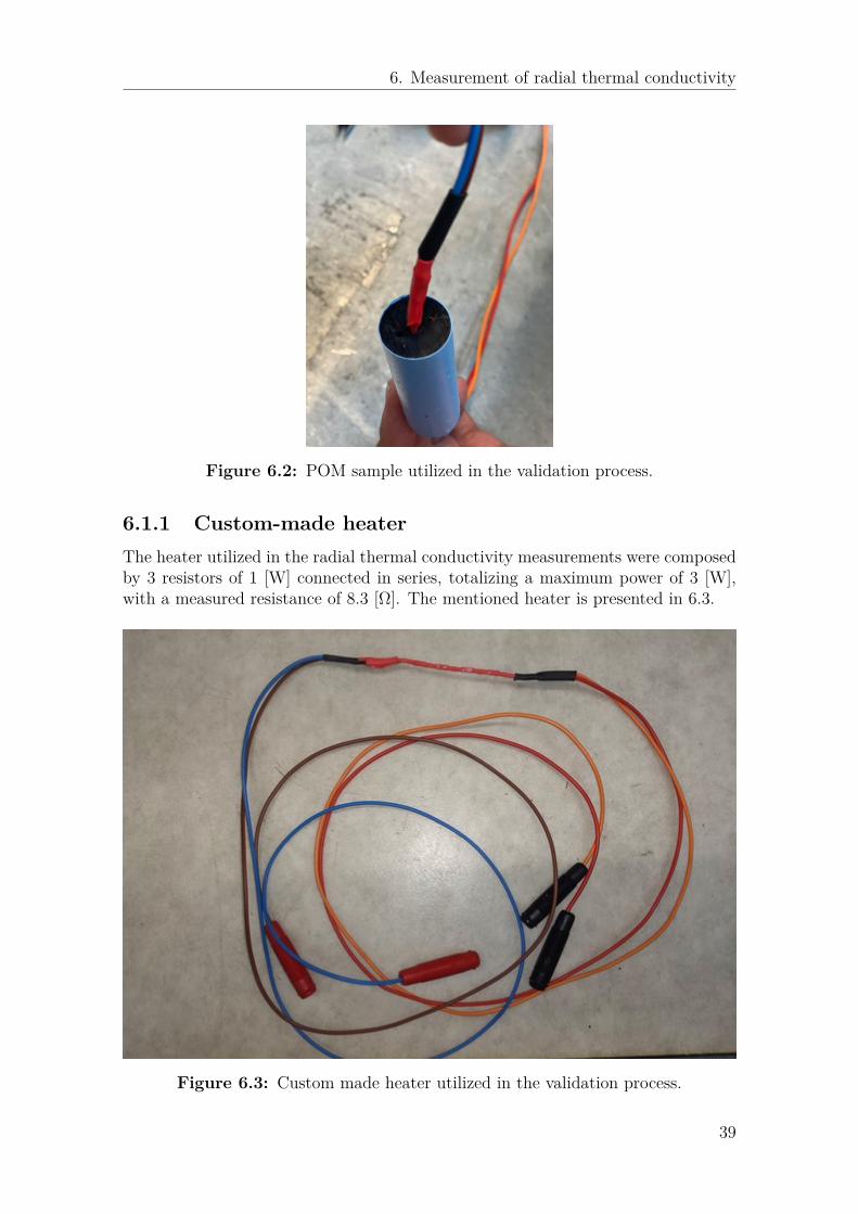
Thus, a 3 mm thick hole was drilled through the sample’s centre, and a 2.5 mmthick hole was drilled at ∆x mm from the sample’s surface. The hole in the centrepassed through the entire sample, and the other one was 5mm deep. A custom-madeheater, described in Section 6.1.1, was placed in the first hole, and a PT100 tem-perature sensor was placed in the second one. Then, the sample was placed entirelybetween plates set “S”, so the temperature at the sample’s surface would remainconstant (controlled by the heat sinks temperature). Therefore, the heater was re-sponsible for providing the heat flow through the radial direction, since the sample’ssurface and centre temperatures could be considered as constant, and the additionaltemperature sensor would record the temperature from ∆x mm from the sample’ssurface. Similar to what was done for the axial thermal conductivity measurements,the experiments were conduct in cycles, each cycle composed by 2 hours of heateron and 2 hours of heater off (resting period). Figure 6.1 shows a conceptual schemefrom the experimental set-up, and Figure 6.2 shows a picture from the utilized POMsample.

37

6. Measurement of radial thermal conductivity

Assuming a constant heat flow in the radial direction, and that the system is oper-ating in a steady state condition, the equation to calculate the heat flowing throughthe radial direction can be obtained from (2.2). The result is the one-dimensionalsteady state heat conduction equation for the radial direction

qradial = −2 · π ·Kradial · lsample · ∆Tln(

rsample

rsample−∆x

) (6.1)

where, qradial is the heat flow in the radial direction [W], Kradial is the radial thermalconductivity [W/(m.K)], lsample is the samples’s length [m], ∆T [K] is the temper-ature difference between ∆x mm from the sample’s surface (T1) and the sample’ssurface (T2), ∆x is distance between the temperature sensor and the sample’s sur-face [m], and rsample is the sample’s radius. Therefore, Kradial can be calculatedas

Kradial =∣∣∣∣∣− qradial · ln

(rsample

rsample−∆x

)2 · π · lsample · ∆T

∣∣∣∣∣ (6.2)

Figure 6.1: Conceptual scheme from the experimental set-up for the radialthermal conductivity measurements.

38


Figure 6.2: POM sample utilized in the validation process.

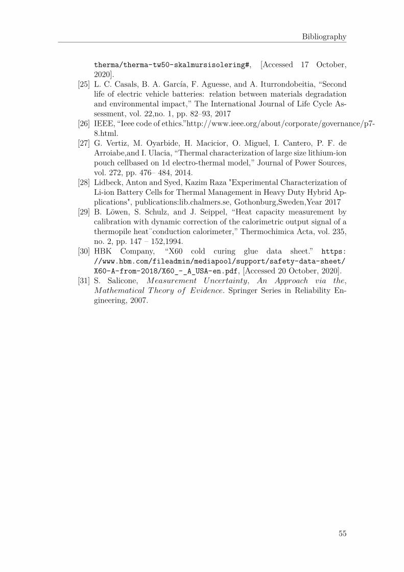
6.1.1 Custom-made heaterThe heater utilized in the radial thermal conductivity measurements were composedby 3 resistors of 1 [W] connected in series, totalizing a maximum power of 3 [W],with a measured resistance of 8.3 [Ω]. The mentioned heater is presented in 6.3.

Figure 6.3: Custom made heater utilized in the validation process.

39


6.2 ValidationThe validation process was conducted utilizing a Polyoxymethylene (POM) rod withthe same dimensions of a 21700 cylindrical cell. The experiments were performedaccording to the method described in section 6.1, considering ∆x = 4.5mm. Theused set-up is shown in Figure 6.4, and the experimental results are presented inTable 6.1.

Figure 6.4: Calorimeter set up for the radial thermal conductivity measurements.

Table 6.1: Experimental results for the radial thermal conductivitymeasurements.

Heatpower

Measuredpower


Kr[W/m.K]


∆T[°C]

0.332 0.267 81% 0.341 10% 1.020.401 0.339 84% 0.345 12% 1.280.518 0.424 82% 0.344 11% 1.610.605 0.515 85% 0.341 10% 1.980.747 0.602 81% 0.334 8% 2.370.849 0.720 85% 0.347 12% 2.710.959 0.783 82% 0.354 14% 2.891.016 0.833 82% 0.341 10% 3.19

40


Analysing the results, it is possible to see that the power ration between the appliedpower to the heater and the actual heat being transferred to the sample presentedgood values, being greater than 80%. Regarding the temperature variation, theintention was to keep its value inside of range from 1°C to 3°C, since high valuesof temperature variation could contribute to increase the heat losses, and, as it ispossible to verify in Table 6.1, this measurements were successfully performed forthe mentioned range. Moreover, the values of Kr presented a great consistency, andgood Deviation values in general (below 15%). Therefore, the described method wasconsidered suitable for application in the cell measurements.

41


42

7Results and analysis

The results and analysis of the thermal properties measurements of the cylindricalLi ion battery cell are presented in this chapter. A full description of the cell utilizedin the measurements can be found in Table 7.1, and a picture of the cell can be foundin Figure 7.1.

Table 7.1: Cylindrical cell’s technical description.

Cell model Voltage operationrange [V]

Capacity[Ah]

Dimensions[R x L]mm

Weight[g] Chemistry

TESLA 21700cylindrical cell 2.5 - 4.2 4.5 21x70 69 NCA

Figure 7.1: Tesla cell utilized in the measurements.

43

7. Results and analysis

7.1 Specific heat capacity (Cp)The measurements of the specific heat capacity were performed as described inChapter 4, considering a temperature range from 18°C to 22°C. The obtained spe-cific heat capacity value, together with the respectively measurement variation, arepresented in Table 7.2. The resulting value of Cp can be considered as a reasonableone, since it is close to already reported specific heat capacity values for cylindri-cal Li ion cells, found in the literature [19], [20]. The measurement variation alsopresented a good result, showing a fair level of variation. At last, the acquired ex-perimental data of heat flow and temperature variation, utilized for the cell’s Cp

calculation, are presented in Figure 7.2 and Figure 7.3.

Table 7.2: Specific heat capacity of the 21700 NCA cylindrical Li ion cell.

Measured Value[J/kg.°C]

Measurement variation[J/kg.°C]

841 ±27.1

Figure 7.2: Corrected heat flow signals utilized for the cell’s Cp determination.

7.2 Axial thermal conductivity (Ka)The measurements of the cell’s axial thermal conductivity were performed accord-ing to the method described in Chapter 5 (axial thermal conductivity chapter). Asit can be seen in Table 7.3, the acquired cell’s (Ka value is 6.93 ± 0.1 [W/m.K],which is considerably below the expected axial thermal conductivity value for cylin-drical Li ion cells. Therefore, some modifications were implemented to the originalmethod mentioned in Chapter 5. An extra PT100 temperature sensor was attachedto the cells surface, as shown in Figure 7.4, in order to avoid wrong temperature

44


Figure 7.3: Temperature signals utilized for the cell’s Cp determination.

measurements resulted from the existing close contact between the heater and themodified temperature sensor. Moreover, a new parameter ∆x2 was defined, beingthe distance from the new temperature sensor to the plates set “S”. Regarding Ka

calculations, the path considered for the calculations needed to be changed, in orderto fit the modified experimental set-up. Therefore, the new path considered thedistance between the new temperature sensor to the plates set "S". Furthermore,instead of using ∆x in 5.2, ∆x2 was the utilized distance, and the variation of tem-perature was considered between the new temperature sensor and the average of thetemperature readings from plates SA and SB. At last, a new test was performedbased on the mentioned modifications and considering ∆x2 = 10mm. The resultsare presented in Table 7.4.

Table 7.3: Acquired axial thermal conductivity of the 21700 NCA cylindrical Liion cell without the extra temperature sensor.

Measured Value[W/m.K]

Measurement variation[W/m.K]

6.93 ±0.1

Table 7.4: Axial thermal conductivity value of the 21700 NCA cylindrical Li ioncell considering the extra temperature sensor.



11.55 ±0.1

The result acquired from the modified method is more in agreement with theexpected result for a cylindrical Li ion battery cell, moreover, the measurementvariation also presented a good result, confirming the consistence of the presented

45


Figure 7.4: Additional temperature sensor attached to the cell’s surface.

method. Lastly, Figure 7.5 and Figure 7.6 show 3 of the temperature and correctedheat flow samples utilized for the determination of Ka.

Figure 7.5: 3 Samples of the corrected heat flow signals from the cell’s axialthermal conductivity measurements.

46


Figure 7.6: 3 Samples of the temperature signals from the cell’s axial thermalconductivity measurements.

7.3 Radial thermal conductivity (Kr)The method utilized for the measurements of the radial thermal conductivity of thecylindrical Li ion cell is described in Chapter 6. However, due to technical issues,the heater utilized for the experiments needed to be modified in order to better fitthe cell’s design. The new heater was composed by 2 resistors of 3 [W] connectedin series, with a total measured resistance of 95 [Ω], attached to a cooper rod. Thecooper rod was placed inside of the hole drilled in the cell’s centre. Additionally,another change made was that the hole drilled in the cell’s centre did not passthrough the entire cell, having a total depth of 35mm instead. Before the drillingprocess be performed, due to safety reasons, the cell was completely discharged witha C/10 rate, and short circuited for 1 week, so the cell could be considered electricalinactive. Once the hole for the heater and the temperature sensor were drilled,they were immediately filled up with the X60 cold curing glue [30], produced byHBM, responsible for both filling up the gap left by the drilling, avoiding electrolyteleakage, and also for fixation. Figure 7.7 shows an image from the utilized heater,and Figure 7.8 shows an image from the cell with both the temperature sensor andthe heater already installed. Furthermore, the obtained value of the radial thermalconductivity is shown in Table 7.5.

Table 7.5: Radial thermal conductivity value of the 21700 NCA cylindrical Li ioncell considering.



0.83 ±0.04

Both temperature and heat flow signals were satisfactorily stable during the mea-surements. In addition to that, the resulting value of the cell’s radial thermal con-

47


Figure 7.7: Heater utilized in the measurements of the cell’s radial thermalconductivity.

Figure 7.8: Drilled cell both the temperature sensor and the heater installed.

ductivity presented a very good consistency, as it is possible to see from the valueof the measurement variation. Finally, Figure 7.9 and Figure 7.10 show 3 of thecorrected heat flow and temperature samples utilized for the determination of Kr.

48


Figure 7.9: 3 Samples of the temperature signals from the cell’s radial thermalconductivity measurements.

Figure 7.10: 3 Samples of the corrected heat flow signals from the cell’s radialthermal conductivity measurements.

49


50

8Conclusion

The main focus of this master thesis work was to modify and improve a custom-madeIsothermal Heat Conduction (IHC) calorimeter, designed to operate with prismaticand pouch Li ion cells, in order to be applied in thermal characterization of cylindri-cal Li ion cells. Considering the results obtained, the modifications were successful,and it was proved that the calorimeter is well suitable for the designed task.

Some issues related to heat leakage were faced when the measurements of specificheat capacity were performed, highlighting the importance of having an isothermalenvironment condition secured during the entire test, especially when performingtests that involve considerably low heat flow signals to be measured. It was notedthat even small variations in the temperature outside of the isolation box were inter-fering with the measurements. The issues were overcome by adding a new heat sinkto the calorimeter set-up, and applying the linear temperature increase method, inorder to keep the temperature inside of the box as constant as possible. The mea-sured Cp value of the cylindrical Li ion cell was 841 [J/kg.°C].

The axial thermal conductivity was measured for different power levels, respect-ing a maximum temperature variation range around 3ºC. After applying a betterdesigned heater in the set-up, the resulting measurements from the validation pro-cess presented a really good level of consistency. Regarding the cell’s measurements,the position of the temperature sensor, as well as the length of the cell left outsideof the calorimeter plates, had to be changed, in order to improve the method’s re-liability. The main concern was that the temperature sensor and the heater weretoo close to each other, probably impacting the temperature measurement from thetop of the cell. Once the modifications were applied, the measurements presenteda good consistency, and the measured cell’s axial thermal conductivity was 11.55[W/m.K].

The method for the measurement of the radial thermal conductivity was also vali-dated for different levels of power, respecting 3°C as maximum temperature variationrange. In the validation process, the measurements precision was consistence, pre-senting good results. For the cell’s measurements, the heater needed to be changedto improve its fitting in the cell’s centre drilled hole. The strategy of drilling theholes in the cell was successfully applied, having almost no lost of electrolyte. Themeasured value of the cylindrical cell radial thermal conductivity was 0.83 [W/m.K],presenting a really good precision.

51

8. Conclusion

As expected, the axial thermal conductivity of the cylindrical cell is considerablyhigher than the radial one, due to the fact that in the radial direction, the heat mustflow through several layers of materials (cell’s active materials, separator, etc), andsome of these materials are poor heat conductors, while in the axial direction, theheat will mainly flow through the materials that have the highest thermal conduc-tivities (Aluminium or Copper).

This thesis work presented methods that can be used for the thermal characteri-zation of cylindrical Li ion cells utilizing an IHC calorimeter. The obtained resultsshowed a very good precision, and can be considered has a valuable contribution forthermal management of Li-ion battery packs, since the presented thermal parame-ters can be applied into further studies, helping to improve the battery managementsystem as whole.

8.1 Future workFuture investigations are necessary to validate the kinds of conclusions that can bedrawn from this study. There are quite a few areas in this thesis work that can beimproved in the future. For more accuracy of the measurements or improvement ofthe method below suggestions can be implemented in the future.

• Though having a styrofoam box as insulation for the setup, the inside boxtemperature was affected by the room temperature. Therefore, the setup canbe used inside a new styrofoam box or temperature chamber for getting aconsistent temperature around the setup. On the other hand, instead of onecooling plate inside the box, more coolings palates can be used for gettingstable temperature around the setup.

• Modified IHC made for only two samples, one more pair of pressure plates (forone sample) can be added in calorimeter for having more accurate measure-ments.

• The result can be validated by simulation which could be done in ComsolMultiphysics. In order to achieve a more desirable result for designing a coolingsystem model should more be constructed. As well, the model could be coupledwith an electrical model.

• In Future work should consider the potential effects of the low power ratiobetween the applied power from the heater and actual heat being transferredto the sample in Ka ( axial thermal conductivity measurement method). Moreimproved/modified heater could be used to utilize maximum power from theheater to the sample.

• For more understanding of the behavior and the cell, the dependency of ther-mal properties on temperature, cell SOC and SOH can be further studied.

52

Bibliography

[1] T. L. Bergman, A. S. Lavine, F. P. Incropera and D. P. Dewitt,Fundamentals of heat and mass transfer, 7th edition, 2011.

[2] A. Lidbeck and K. R. Syed, "Experimental Characterization of Li-ionBattery cells for Thermal Management in Heavy Duty Hybrid Appli-cations", Department of Energy and Environment − Division ofElectric Power Engineering, CHALMERS university of technology,2017.

[3] C. Zhao, W. Cao, T. Dong and F. Jiang, "Thermal behavior study of dis-charging/charging cylindrical lithium-ion battery module cooled by chan-neled liquid flow", International Journal of Heat and Mass Transfer,vol. 120, pp 751–762, 2018.

[4] W. Cao, C. Zhao, Y. Wang, T. Dong and F. Jiang, "Thermal model-ing of full-size-scale cylindrical battery pack cooled by channeled liquidflow", International Journal of Heat and Mass Transfer, vol. 138, pp1178–1187, 2019.

[5] B. Ng, P. T. Coman, W. E. Mustain and R. E. White, "Non-destructiveparameter extraction for a reduced order lumped electrochemical-thermalmodel for simulating Li-ion full-cells", Journal of Power Sources, vol.445, 227296, 2020.

[6] S. Wang, K. Li, Y. Tian, J. Wang, Y. Wu and S. Ji, "An experimental andnumerical examination on the thermal inertia of a cylindrical lithium-ionpower battery", Applied Thermal Engineering, vol. 154, pp 676–685,2019.

[7] D. Stephens, P. Shawcross, G. Stout, E. Sullivan, J. Saunders, S. Risser,and J. Sayre, "Lithium-ion battery safety issues for electric and plug-inhybrid vehicles",Washington, DC : National Highway Traffic SafetyAdministration., 261 pages, 2017.

[8] H. Berg, "Batteries for electric vehicles: Materials and electrochemistry",Cambridge University Press, 250 pages, 2015.

[9] S. J. Drake, D. A. Wetz, J. K. Ostanek, S. P. Miller, J. M. Heinzel andA. Jain, "Measurement of anisotropic thermophysical properties of cylin-drical Li-ion cells", Journal of Power Sources, vol. 252, pp 298–304,2014.

[10] X. Lin, H. E. Perez, S. Mohan, J. B. Siegel, A. G. Stefanopoulou, Y.Ding and M. P. Castanier, "A lumped-parameter electro-thermal modelfor cylindrical batteries", Journal of Power Sources, vol. 257, pp 1–11,2014.

53

Bibliography

[11] T. S. Bryden, B. Dimitrov, G. Hilton, C. P. León, P. Bugryniec, S. Brown,D. Cumming and A. Cruden, "Methodology to determine the heat capac-ity of lithium-ion cells", Journal of Power Sources, vol. 395, pp 369–378,2018.

[12] H. Zhou, F. Zhou, Q. Zhang, Q. Wang and Z. Song, "Thermal manage-ment of cylindrical lithium-ion battery based on a liquid cooling methodwith half-helical duct", Applied Thermal Engineering, vol. 162, 114257,2019.

[13] J. Cao, M. Luo, X. Fang, Z. Ling and Z. Zhang, "Liquid cooling withphase change materials for cylindrical Li-ion batteries: An experimentaland numerical study", Energy, vol. 191, 116565, 2020.

[14] S. Zhu, J. Han, H. Y. An, T. S. Pan, Y. M. Wei, W. L. Song, H. S. Chenand D. Fang, "A novel embedded method for in-situ measuring internalmulti-point temperatures of lithium ion batteries", Journal of PowerSources, vol. 456, 227981, 2020.

[15] S. Zhu, J. Han, T. S. Pan, Y. M. Wei, W. L. Song, H. S. Chen and D.Fang, "A novel designed visualized Li-ion battery for in-situ measuringthe variation of internal temperature", Extreme Mechanics Letters, vol.37, 100707, 2020.

[16] C. Forgez, D. V. Do, G. Friedrich, M. Morcrette and C. Delacourt, "Ther-mal modeling of a cylindrical LiFePO4/graphite lithium-ion battery",Journal of Power Sources, vol. 195, pp 2961–2968, 2010.

[17] W. Zielenkiewicz and E. Margas, Theory of Calorimetry. Hot Topics inThermal Analysis and Calorimetry, Springer Netherlands, 2002.

[18] P. M. Gomadam, R. E. White and J. W. Weidner, Theory of Calorime-try. "Modeling Heat Conduction in Spiral Geometries", Journa of theElectrochemical Society, pp A1339-A1345, 2003.

[19] T. S. Bryden, B. Dimitrov, G. Hilton, C. P. de León, P. Bugryniec, S.Brown, D. Cumming and A. Cruden, "Methodology to determine theheat capacity of lithium-ion cells", Journal of Power Sources, vol. 395,pp 369–378, 2018.

[20] K. A. Murashko, J. Pyrhönen and J. Jokiniemi, "Determination of thethrough-plane thermal conductivity and specific heat capacity of a Li-ioncylindrical cell", International Journal of Heat and Mass Transfer,vol. 162, 120330, 2020.

[21] Julabo USA Inc, “Data sheet for JULABO F25MA.” http://www.julabo.cn/uploadfile/2018/0411/JULABO-F25-MA--9153625.pdf.[Accessed 16 October, 2020].

[22] Gamry Instruments, Inc., “Reference 3000 potentiostat/galvanos-tat/zra operator´s manual.” https://www.gamry.com/assets/Uploads/Reference-3000-Operators-Manual.pdf, [Accessed 16 October, 2020].

[23] Pico technology, “PT-104 data logger.” https://www.picotech.com/download/datasheets/pt-104-prt-data-logger-data-sheet.pdf,[Accessed 16 October, 2020].

[24] Kingspan Insulation AB, “Therma TW50 insulation plates informa-tion.” https://www.kingspan.com/se/sv-se/produkter/isolering/

54

http://www.julabo.cn/uploadfile/2018/0411/JULABO-F25-MA--9153625.pdf

http://www.julabo.cn/uploadfile/2018/0411/JULABO-F25-MA--9153625.pdf

https://www.gamry.com/assets/Uploads/Reference-3000-Operators-Manual.pdf

https://www.gamry.com/assets/Uploads/Reference-3000-Operators-Manual.pdf

https://www.picotech.com/download/datasheets/pt-104-prt-data-logger-data-sheet.pdf

https://www.picotech.com/download/datasheets/pt-104-prt-data-logger-data-sheet.pdf

https://www.kingspan.com/se/sv-se/produkter/isolering/therma/therma-tw50-skalmursisolering#



Bibliography

therma/therma-tw50-skalmursisolering#, [Accessed 17 October,2020].

[25] L. C. Casals, B. A. García, F. Aguesse, and A. Iturrondobeitia, “Secondlife of electric vehicle batteries: relation between materials degradationand environmental impact,” The International Journal of Life Cycle As-sessment, vol. 22,no. 1, pp. 82–93, 2017

[26] IEEE, “Ieee code of ethics.”http://www.ieee.org/about/corporate/governance/p7-8.html.

[27] G. Vertiz, M. Oyarbide, H. Macicior, O. Miguel, I. Cantero, P. F. deArroiabe,and I. Ulacia, “Thermal characterization of large size lithium-ionpouch cellbased on 1d electro-thermal model,” Journal of Power Sources,vol. 272, pp. 476– 484, 2014.

[28] Lidbeck, Anton and Syed, Kazim Raza "Experimental Characterization ofLi-ion Battery Cells for Thermal Management in Heavy Duty Hybrid Ap-plications", publications:lib.chalmers.se, Gothonburg,Sweden,Year 2017

[29] B. Löwen, S. Schulz, and J. Seippel, “Heat capacity measurement bycalibration with dynamic correction of the calorimetric output signal of athermopile heat¨conduction calorimeter,” Thermochimica Acta, vol. 235,no. 2, pp. 147 – 152,1994.

[30] HBK Company, “X60 cold curing glue data sheet.” https://www.hbm.com/fileadmin/mediapool/support/safety-data-sheet/X60-A-from-2018/X60_-_A_USA-en.pdf, [Accessed 20 October, 2020].

[31] S. Salicone, Measurement Uncertainty, An Approach via the,Mathematical Theory of Evidence. Springer Series in Reliability En-gineering, 2007.

55




https://www.hbm.com/fileadmin/mediapool/support/safety-data-sheet/X60-A-from-2018/X60_-_A_USA-en.pdf



Bibliography

56

AAppendix 1

A.1 Measurement variation calculationsFor the calculations of variation for all the three thermal properties presentedin this thesis, the standard deviation value was utilized to define the variationvalues. Considering a group with n samples, the standard deviation value (S)can be calculated as [31]

S =√√√√ n∑

i=1

(xi − x)2

n(A.1)

where x is the average value of the sample’s group, n is the total number ofsamples and xi represents each of the samples within the group. Lastly, theaverage value of a data group, composed by n samples, can be calculated as

x =n∑

i=1

xi

n(A.2)

A.1.1 Specific heat capacity (Cp)For the calculation of the measurement variation regarding the cell’s specificheat capacity, the samples presented in Table A.1 were utilized.

Table A.1: Utilized samples in the calculation of Cp measurement variation.

Sample index (i) Cp [J/kg.ºC]1 8.28E+022 8.70E+023 8.08E+024 8.57E+025 8.29E+026 8.52E+027 8.12E+028 8.62E+029 8.02E+0210 8.85E+02

Applying the data set presented in Table A.1 into (A.1) and (A.2) resulted inx = ∑n

i=1xi

n= 8.28×102+8.70×102+...+8.85×102

10 = 8.41 × 102[ Jkg.°C ]

I

A. Appendix 1

S =√

(8.28×102−8.41×102)2+...+(8.85×102−8.41×102)2

10 = 27.1[ Jkg.°C ]

A.1.2 Axial thermal conductivity (Ka)For the calculation of the measurement variation regarding the cell’s axialthermal conductivity before adding the extra temperature sensor, the samplespresented in Table A.2 were utilized.

Table A.2: Utilized samples in the calculation of Ka measurement variation.

Sample index (i) Ka [W/m.K]1 6.752 6.803 6.844 6.845 6.856 6.887 6.888 6.939 6.9510 6.9611 6.9712 6.9113 7.0114 7.0315 7.0716 7.14

Applying the data set presented in Table A.2 into (A.1) and (A.2) resulted in

x = ∑ni=1

xi

n= 6.75+6.80+...+7.14

16 = 6.93[ Wm.K

]

S =√

(6.75−6.93)2+(6.80−6.93)2+...+(7.14−6.93)2

16 = 0.1[ Wm.K

]

Furthermore, the calculation of the measurement variation regarding the cell’saxial thermal conductivity, considering the extra temperature sensor, wereperformed considering the samples presented in Table A.3.


x = ∑ni=1

xi

n= 11.67+11.71+...+11.71

16 = 11.55[ Wm.K

]

S =√

(11.67−11.55)2+(11.71−11.55)2+...+(11.71−11.55)2

16 = 0.1[ Wm.K

]

II

A. Appendix 1

Table A.3: Utilized samples in the calculation of Ka measurement variation.

Sample index (i) Ka [W/m.K]1 11.672 11.713 11.734 11.745 11.716 11.357 11.398 11.409 11.4110 11.4211 11.4412 11.7113 11.4714 11.4915 11.4516 11.71

A.1.3 Radial thermal conductivity (Kr)For the calculation of the measurement variation regarding the cell’s radialthermal conductivity, the samples presented in Table A.4 were utilized.

Table A.4: Utilized samples in the calculation of Cp measurement variation.

Sample index (i) Kr [W/m.K]1 0.792 0.843 0.874 0.895 0.856 0.777 0.788 0.789 0.8210 0.84


x = ∑ni=1

xi

n= 0.79+0.84+...+0.84

10 = 0.83[ Wm.K

]

S =√

(0.79−0.83)2+(0.84−0.83)2+...+(0.84−0.83)2

10 = 0.04[ Wm.K

]

III

Date post:	23-Feb-2022
Category:	Documents
Upload:	others
View:	4 times
Download:	0 times

Thermal Characterization of a Cylindrical Li-ion Battery Cell

Documents