Thermal collapse of a granular gas under gravity Baruch Meerson

Hebrew University of Jerusalem

in collaboration with

Dmitri Volfson - UCSDLev Tsimring - UCSD

Support:US DOEIsrael Science FoundationGerman-Israeli Foundation for Scientific Research and Development

Southern Workshop on Granular Materials, Viña

del Mar, 2006

Phys. Rev. E 73, 061305 (2006)

Granular gas: instantaneous inelastic binary collisions

1r0 (constant) coefficient of normal restitution

Momentum preserved, part of kinetic energy lost

Simplest model of granular flow

tangential velocitycomponents:

normal velocitycomponents:

Continuum modeling: hydrodynamics of dilute granular gases at q=(1-r)/2 << 1

P: stress tensor Q: heat flux ~ (1-r2) n2 T3/2: rate of energy loss by inelastic

collisions (Haff 1983)

. Γ:)(t

,)(t

, 0)(t

vPQv

gPvvv

v

TT

n

nn

nn

Constitutive relations are derivable from the Boltzmann equation(generalized to account for inelastic collisions)

under scale separation: mean free path << hydrodynamic length scales

Bulk energy losses

mass conservation

momentum conservation

energy balance

Homogeneous Cooling State: a paradigm of kinetic theory and hydrodynamics

20

0

)/1(),(

tt

TtT

r Haff’s law

2/100

20)1(

2

Tdnrt

cooling time in two dimensions

n(r,t) = n0 = const

v(r,t) = 0

d: particle diameter particle mass=1

g=0

How does gravity modify the cooling dynamics?

Qualitative picture: gravity forces grains to sink to the bottom of thecontainer, where increased density enhances the collision rate and causes“freezing” of the granulate. Surprisingly, no quantitative analysis has ever been performed.

We combined MD simulations and numerical and analytical solutions ofhydrodynamic equations to develop a detailed quantitative understanding of the cooling process.

Main result: in contrast to Haff's law, the cooling gas undergoes thermal collapse: it cools down to zero temperature and condenses on the bottom plate in a finite time exhibiting, close to collapse, a universal scaling behavior.

Why should we care? 1. A non-trivial test of hydrodynamics2. Aesthetic beauty

Event-driven MD simulations

Circles: Total kinetic energy normalized to value at t=0

Total kinetic energy drops to zero in a finite time tc. Apparent scaling ~ (tc-t)2 close to tc.

N=5642, Lx=102, r=0.995, T0=10, g=0.01t=0: barometric density profile

Dash-dot: same for adifferent initial condition units of time: see later

Hydrodynamic theory deals with hydrodynamic fields n(y,t), T(y,t) and v(y,t)

'),'(),(0y

dytyntym mass content between the bottom plateand the (Eulerian) point y

One-dimensional time-dependent flow: easier to solve using the Lagrangian coordinate

y: vertical coordinate

Having solved the problem in the Lagrangian coordinates [that is, having

found n(m,t), T(m,t) and v(m,t)], we can return to the Eulerian coordinate y:

m

tmn

dmtmy

0

.),'(

'),(

.4-3

4)v(

2v

),v(2

1)(v

v1

3/222/322/12

2/12

t2

nTTnnTnTT

nTnT

n

mmmmt

mmm

mt

./vv

,/

,/

)/(,/

/,/

0

2/11

0

d

x

dd

t

TTT

NLnn

gtttt

gTyy

gravity length scale at t=0

relative role of heat losses and heat conduction

Hydrodynamic equations

Λ2=(1-r2)/(4ε2)

Two scaled parameters

ε ~1/( number of granular layers at rest( ε<<1 guarantees td>>(λ/g)1/2

ε = π-1/2Lx/(Nd)<<1

Bromberg,Livne andMeerson (2003)

'),'(),(0y

dytyntym

Lagrangian mass coordinate

Boundary conditions: zero fluxes of mass, momentum and energy at y=0 and y=∞ (that is, at m=0 and m=1).

heat diffusion time

Numerical solution of hydrodynamic equations A variable mesh/variable time step solver (Blom and Zegeling).

Short-time behavior is

complicated: shock waves emerge

and heat the gas at large heights.

Circles: MD simulationsBlack solid line: hydrodynamics

N=5642, Lx=102, r=0.995,T0=10, g=0.01

Hydrodynamic parameters ε=0.01 and Λ=6

t=0: barometric density profile

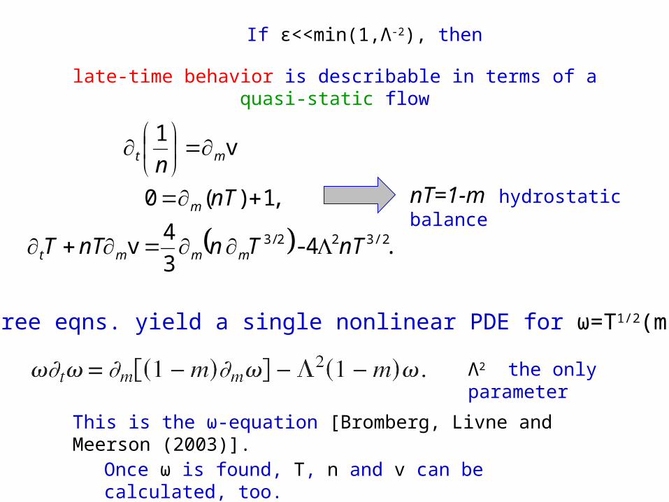
late-time behavior is describable in terms of a quasi-static flow

.4-3

4v

,1)(0

v1

3/222/3 nTTnnTT

nT

n

mmmt

m

mt

If ε<<min(1,Λ-2), then

These three eqns. yield a single nonlinear PDE for ω=T1/2(m,t):

This is the ω-equation [Bromberg, Livne and Meerson (2003)].

nT=1-m hydrostatic balance

Λ2 the only parameter

Once ω is found, T, n and v can be calculated, too.

Numerical solution of the ω-equation Same variable mesh/variable time step solver

Computations launched at scaled time t=0.04 when the flow is already quasi-static. Temperature profile produced by the full hydrodynamic solver used as initial condition.

Circles: MD simulationsBlack solid line: hydrodynamicsRed dashed line: ω-equation

Λ=6, T(m,t=0)=1

Numerical solution of the ω-equation Another example: Λ=1, T(m,t=0)=1

Simulations performed at different Λ and different initial conditions. Thermal collapse

always observed at a finite time tc which goes down as Λ increases. T(m,t) vanishes, at t=tc ,

on the whole Lagrangian interval 0<m<1, while the density n=(1-m)/T blows up there. At

t=tc this Lagrangian interval corresponds to a single Eulerian point y=0. Therefore, all of the

gas condenses at the bottom plate and cools to zero temperature at t=tc.

Analytic theory

t)Q(m),(tω(m,t) c

Remarkably, close to collapse the solution of the initial value problem for the ω-equation becomes separable:

Q(m) is determined by the nonlinear ordinary differential equation

and the boundary conditions (1-m)Q'(m)=0 at m=0 and m=1.

The function Q(m) is uniquely determined by Λ and, for each Λ, can be found numerically, by shooting. The collapse time tc depends on the initial condition.

that is, .22 (m)Qt)(tT(m,t) c

Λ2<<1: perturbation theory

Here one can show that Q(m) ~ Λ2<<1 Furthermore, as heat conduction dominates over heat losses, the solution must be almost uniform in space, and we arrive at

This solution is in excellent agreement with numerical one at Λ2<1.

Λ2>>1

Here we stretch the coordinate and time in the ω-equation: ξ=Λ(1-m) and τ=Λt.

The equation becomes

while Λ determines the interval: 0 < ξ ≤ Λ. The separable solution is

),)q((),ω( c while the boundary value problem for q(ξ) is the following:

At ξ>>1 (that is, everywhere except the boundary layer at m=1) q(ξ) is exponentially small, and one can drop the term q2. The resulting linear equation solvable in Bessel functions.

Envelope corresponds to limit Λ→∞

Physics: q2-term comes from ωωt. At Λ>>1 the energy losses are balanced by heat conduction everywhere, except at very high altitudes. The high altitudes serve as a dynamic bottleneck of the cooling process.

We have also found approximate analytical solutions for the initial stage of the slow cooling, at large and small Λ, and determined the

collapse time tc = tc(Λ)

For concreteness, isothermal (barometric) density profile at t=0is assumed.

Details: D.Volfson, B. Meerson and L.S. Tsimring, Phys. Rev. E 73, 061305 (2006)

A summary of collapse properties

)()1(

2

2

t)(t

mQmn(m,t)

c

22 (m)Qt)(tT(m,t) c

.)'()'1(

'2

02

m

c mQm

dmt)(tv(m,t)

The temperature vanishes at t=tc:

The density blows up

The gas velocity is

Though v(m,t) is zero everywhere at t=tc, the gas flux nv blows up.

This happens on the whole Lagrangian interval 0<m<1, but this interval corresponds to a single Euleiran point y=0. That is, at t=tc all of the gas condenses on the bottom plate and cools to zero temperature.

What is the total kinetic energy of all particles as a function of time?

.)(~'),'()2/1(),'(

dy' ),'()2/1(),'(),'()(

21

0

2

0

2

ttdmtmvtmT

tynvtyTtyntE

c

Compare to Haff’s law

20

0

)/1()(

tt

EtEH

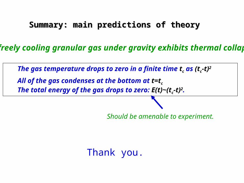
Summary: main predictions of theorySummary: main predictions of theory

The gas temperature drops to zero in a finite time tc as (tc-t)2

All of the gas condenses at the bottom at t=tc

The total energy of the gas drops to zero: E(t)~(tc-t)2.

Thank you.

Should be amenable to experiment.

A freely cooling granular gas under gravity exhibits thermal collapse