Signature of Author'b-fDer ent of Ocean Engineering
7 May 1993
Certified byKoichi Masubuchi
Kawasaki Professor of EngineeringDepartment of Ocean Engineering, Thesis Supervisor
Department of Materials Science and Engineering, Thesis Supervisor
Accepted byLinn W. Hobbs
John F. Elliot Professor of MaterialsChair, Departmental Committe on. Graduate Students
Accepted by--Professor A. L5I6ug-aiCilichael
: Chairman, Department Graduate CommitteeDepartment of Ocean Engineering
Is?. . 1 995
THERMAL INSULATION OF
WET SHIELDED METAL ARC WELDS
byPatrick Joseph Keenan
Submitted to the Departments of Materials Science and Engineering and Ocean
Engineering on May 7, 1993 in partial fulfillment of the requirements for the degrees of
Master of Science in Materials Engineering and Naval Engineer
ABSTRACT
Computational and experimental studies were performed to determine the effect of staticthermal insulation on the quality of wet shielded metal arc welds (SMAW). Acommercially available heat flow and fluid dynamics spectral-element computer programwas used to model a wet SMAW and to determine the potential effect on the weldcooling rate of placing thermal insulation adjacent to the weld line. Experimental manualwelds were made on a low carbon equivalent (0.285) "mild steel" and on a higher carbonequivalent (0.410) "high tensile strength" steel, using woven fabrics of alumina-boria-silica fibers to insulate the surface of the plate being welded. The effect of the insulationon weld quality was evaluated through the use of post-weld Rockwell Scale hardnessmeasurements on the surface of the weld heat affected zones (HAZs) and by visualinspection of sectioned welds at 10 X magnification.
The computational simulation demonstrated a 150% increase in surface HAZ peaktemperature and a significant decrease in weld cooling rate with respect to uninsulatedwelds, for welds in which ideal insulation had been placed on the base plate surfaceadjacent to the weld line. Experimental mild steel welds showed a reduction in surfaceHAZ hardness attributable to insulation at a 77% significance level. A visual comparisonof the cross-sections of two welds made in 0.410 carbon equivalent steel-withapproximately equivalent heat input-revealed underbead cracking in the uninsulatedweld but not in the insulated weld.
This work has lead to the filing of a patent through the Technology Licensing Office ofthe Massachusetts Institute of Technology and to the initiation of a developmentalresearch project by the Underwater Ship Husbandry branch of the United States NavalSea Systems Command.
Thesis Supervisor: Koichi MasubuchiTitle: Professor of Ocean Engineering and Material Science and Engineering
ACKNOWLEDGMENTS
I wish to thank the following people for the assistance that they provided during
the course of my research.
Mr. Robert Murray of the Naval Sea Systems Command for his logistic support of
my experimental work.
Mr. Gokhan Goktug of MIT who helped me set up the experiment, and patiently
recorded experimental parameters while I welded.
My thesis advisor, Professor Masubuchi, for being constantly available to offer
guidance and advice.
Finally, my wife, Jean M. Fiore, for her patience and editorial skills, both of
which I relied on heavily during the preparation of this manuscript.
TABLE OF CONTENTS
A BSTRA CT .................................................................................................................. 2
ACKNOW LED GM ENTS ............................................................................................ 3
TABLE OF CONTENTS ......................................................................................... 4
LIST O F TABLES .................................................................................................. 6
LIST O F FIG U R ES ....................................................................................................... 7
Underwater welding processes are classified as dry or wet based on exposure to
the ambient environment. Processes that are physically protected from the surrounding
water are classified as dry, whereas wet welding processes are those in which the weld is
directly exposed to the underwater environment.Four dry welding processes are currently in use [1]:
* One-Atmosphere Welding. One-atmosphere welding is performed in a pressure vesselat approximately one atmosphere absolute. Welders who are not trained divers canperform this type of welding after being transferred to the pressure vessel.* Habitat Welding. Welding performed in open-bottom chambers by divers who haveremoved their diving equipment is classified as habitat welding. In both one-atmosphere
and habitat welding, a complete atmosphere conditioning system must be used inconjunction with the chamber or habitat. Welding and respiratory exhaust gases must bevented, and breathing gas supplied to the artificial environment.* Dry Chamber Welding. Dry chamber welding is performed by a diver in divingequipment in an open-bottom enclosure. Full atmosphere condidioning systems are not
required for dry chamber welding since breathing gases are supplied via the diving
equipment. However, diver and welding exhaust gases must be vented from thesechambers to prevent explosions and loss of chamber seal from over-pressurization. Gasmetal arc (GMA), gas tungsten arc (GTA), and shielded metal arc (SMA) processes canbe used in dry chambers as well as in one-atmosphere pressure vessels and habitats.
Electrical resistance pre- and post-heating can also be used in these environments.
* Dry Spot Welding. Dry spot welding is a process in which water is displaced from thelocal weld area by a transparent gas-filled box or via shielding gas surrounded by a
concentric ring of water jets. Divers move the dry box or water-jet welding apparatusalong the joint as the weld is made. Dry box welding is inherently suited to the gas metal
arc welding (GMAW) process because the filler wire can be fed continuously through the
center of the gas box or water-jet to the weld. Welds made with the dry spot process
cannot be pre- or post-heated because the only section of these welds that is isolated from
the water is the area adjacent to the arc.In the case of wet welding, the only viable process for making linear joints that
has been developed to date is shielded metal arc welding (SMAW). (Friction stud
welding has been used with considerable success to make wet spot welds). In wet
SMAW, an arc is struck in the water between an electrode and the surface being welded.
Divers move the electrode along the weld line. No active thermal treatment of wet welds
is feasible because of their direct exposure to the underwater environment.
1.1 Comparison of Wet and Dry Underwater Welding ProcessesWet welding is generally faster and less expensive than dry underwater welding.
The former can be performed on structures of any shape and in confined areas. The
pressure vessels, habitats and cofferdams required for most dry underwater welding
procedures may be difficult or impossible to install on geometrically complex structures
or in physically restricted areas. Fabrication and installation of these enclosures is time
consuming and expensive. Dry spot welding equipment is also more expensive than the
equipment required for wet SMAW. Thus, wet welding is suited for quick inexpensive
repairs.
Wet welding is not as versatile as dry underwater welding with respect to the
variety of processes that can be performed (i.e., GMAW, GTAW, SMAW). However,
since most underwater structures are built with relatively thick material and diver or
remotely operated vehicle (ROV) time at depth is expensive, high deposition rate
processes are required for underwater welding. Therefore, even in enclosures where
GMAW and GTAW could be used, SMAW is the most frequently used welding process.
The primary disadvantage of wet SMAW is that direct exposure to water
deleteriously affects weld quality and limits the types of materials that can be joined.
1.2 Applications of Underwater Welding Procedures
Currently, critical welds such as joints in primary strength members of offshore
structures, pressurized pipeline joints, and hull integrity seams on ships and submarines
are made with dry underwater procedures. Quality cannot be compromised in these
applications so wet SMAW cannot be used. Additionally, welding of high yield strength
steels must be accomplished with dry procedures irrespective of the joint application. No
wet SMAW process has been developed that will produce satisfactory joints in these
materials. Wet SMAW is used only for non-critical or temporary joints in mild steel
structures. Industrial use of wet SMAW is found in secondary structural member joints
on offshore platforms, installation of temporary patches and lifting points in marine
salvage, and construction and repair of coastal zone structures (i.e., piers and
breakwaters).
Underwater welding is commonly employed in the commercial and military
sectors of the maritime industry. Oceaneering Inc., a company that performs contracted
underwater repair services on offshore petroleum and natural gas platforms and pipelines,
and on ships, billed customers for approximately 5 million dollars of underwater welding
services in fiscal year 1992.
The U.S. Navy spent 3.3 million dollars on underwater weld repairs over the
1989-92 period. Fifty percent of these expenditures were for wet welds. Because of their
poor quality, the Navy has classified all wet welds as temporary repairs with the
exception of one non-critical application: the sealing of hull openings in ships that are
being de-commissioned. Consequently, all wet welds made on active Navy ships and
submarines must eventually be removed and replaced by either dry underwater welds or
welds made in drydock.
The expense incurred as a result of reworking temporary wet welds is significant.
Drydocking costs for naval surface combatants range from approximately 250,000 to 1.5
million fiscal year 1992 dollars ($ FY '92). Submarine drydocking costs are on the order
of 1 million $ FY '92. These are costs only for docking and undocking the vessel, and do
not include direct or indirect costs of the repair work. Additionally, drydocking vessels
for replacement of temporary weld repairs disrupts fleet employment and maintenance
schedules.
An advance in technology that improved the quality and scope of wet SMA welds
so that permanent wet welds could be used in more critical applications and on more
materials could provide substantial cost savings to industry and the military.
CHAPTER 2. BACKGROUND
The primary construction material used in the marine environment is steel.
Consequently, only welding of steel will be considered in this thesis. Several processes
have been developed for welding steel in a dry environment: GMAW, GTAW, SMAW
and submerged arc welding. Because of their relatively low metal deposition rates for
manual welding, and the difficulty of displacing water with pressurized shielding gases,
GMAW and GTAW are not suited for wet underwater welding. Submerged arc welding
offers a high deposition rate but covering a joint--even with a hydrophobic flux, if one
could be developed-and maintaining joint coverage in a moving fluid environment
would be difficult, especially when most joints made underwater are either in vertical or
overhead positions. Therefore, wet welding is currently performed almost exclusively
using the SMAW process. The equipment and procedures used for wet SMAW are quite
similar to those used for SMAW in air. The most significant difference is that specialized
electrodes have been developed for wet SMAW. Additionally, power supplies for
underwater SMAW must be capable of moving sufficient current through the relatively
long welding leads that are required because of the separation of the power source from
the submerged work-site.
2.1 Technical Problems Associated With Wet SMA WeldsWet SMA welding arcs are protected from the surrounding water by a bubble of
gas produced by the decomposition of the electrode flux. The flux heat of vaporization is
provided by resistive heating of the electrode when welding current is flowing. The weldpuddle directly behind the arc is re-exposed to the surrounding water immediately after
arc passage. Consequently, unlike welds made in air, wet SMA welds are subjected torapid cooling known as quenching. Quenching is the primary cause of poor quality in wetSMA welds.
Quenching causes the formation of martensite in the heat affected zone (HAZ) of
the weld. The HAZ is the section of the weld that has been heated to above the Al
transformation temperature (723 degrees C) but has not reached the melting point. If therate of cooling from the transformation temperature to ambient temperature is sufficientlyrapid, a needle-like structure called martensite will be formed. The crystal structure of un-tempered martensite inhibits dislocation movement. Consequently, this form ofmartensite is non-ductile.Untempered martensitic HAZs cause welds to be brittle, hard,and to lack toughness.
Arc electrolysis produces atomic hydrogen and oxygen which diffuse into the
weld pool. Quenching traps these gases in the weld because the outward diffusion rate
through the rapidly solidifying metal is much slower than initial diffusion into the molten
weld pool. Entrapped hydrogen reduces weld ductility through the "cold cracking"
mechanism. Over time, hydrogen atoms in the weld migrate to interstitial voids where
they recombine to form hydrogen gas. Pockets of hydrogen gas produce tensile stresses
that can initiate trans-granular cracks. (This phenomena has been termed cold cracking
because it generally occurs after the weld has cooled to approximately 200 degrees C).
Oxygen in the weld produces pores which reduce strength and toughness.
Quenching also traps non-gaseous contaminants such as oxide slags in the weld
metal. These contaminants are generally less dense than iron and would float to the
surface of the weld pool under gradual cooling conditions. Their entrapment further
increases weld porosity.
In addition to micro-structural and chemical effects, quenching produces steep
thermal gradients with resultant high residual stresses, thereby increasing weld
susceptibility to crack initiation upon exposure to environmental loading. Finally,
quenching has been shown to increase weld bead convexity (reinforcement) leaving
welds more susceptible to toe cracking [2].
In summary, wet SMA welds are inherently brittle, porous, and susceptible to
cracking, and all of these traits can be attributed directly or indirectly to rapid weld
cooling.
2.2 Material Limitations of Wet SMA WeldingBecause of weld quenching, wet SMAW cannot be used to join certain materials.
Most important among these are steels that derive their material properties from thermaltreatment (such as quenching and tempering). Low alloy (less than 0.2% carbon), highyield strength, quenched and tempered steels (HY steels) are used widely in theconstruction of naval surface combatants and submarines. Yield strengths of up to 130 ksiare achieved in these steels by quenching low-carbon alloy steel so that a desired amountof martensite is formed. Because of impedance to dislocation flow, martensite is strongbut it has poor toughness. After quenching, the alloy is heated to a maximum temperaturebelow A l, and gradually cooled to ambient temperature. This procedure is known astempering; it causes the martensite to be softened so that toughness is increased, and ifproperly performed can result in only a minor loss of strength. (The temperingtemperature and cooling profile are dependent on the desired mechanical properties of thesteel being produced). The HAZ of an SMA weld made in a high yield strength quenched
and tempered steel will in general have been heated to above the tempering temperature
and then cooled more rapidly than the tempering profile. This is especially true in the
case of wet welds. Consequently, the tempered martensitic structure will have been
transformed into brittle martensite. The result is a non-ductile HAZ that is susceptible to
cracking. In an experiment performed jointly by Batelle Industries and MIT, it was found
that all cracking in experimental HY-80 weldments originated in the HAZ [3]. Cracking
susceptibility is further increased in wet welds because of the relatively large amounts of
hydrogen that they absorb.
In surface welding and dry underwater welding, base plates can be preheated and
post-heated using electrical resistance. These procedures offset HAZ cooling and reduce
or eliminate the loss of toughness in HY steels. Electrical resistance heating of submerged
base plates is not feasible. Hence, because of rapid cooling rates, inability to supply
active heating, and hydrogen absorption, wet SMAW cannot be used to weld quenched
and tempered HY steels.
In addition to HY quenched and tempered steels, martensite is formed in the
HAZs of weldments with relatively high carbon content. Carbon contents of steels are
often compared using an index known as carbon equivalent (CE). (Actually CE is a
measure of both carbon content and, to a lesser extent, the contents of various other
alloying elements. Positive coefficients are assigned to alloying elements that generally
inhibit weldability, and negative coefficients to elements that improve weldability).
Different definitions of CE are encountered in the literature. The most common definition
is presented below in equation (2.1).
%Mn %Cr %Mo %V %Cu %Ni%C++ ----- +-+- {2.1)
6 10 50 10 40 20
The American Welding Society (AWS) has defined a specific relationship to be used
when computing CEs for wet SMAW. This definition--equation (2.2)-is more
conservative (i.e., gives a higher CE for an equivalent material) than equation {2. 1} in
recognition of the technical difficulties associated with wet SMAW.
%Mn %Cr + %Mo + %V %Ni+%Cu%C + - + + -- (2.2)
6 5 15
Masubuchi et. al. demonstrated a direct relationship between carbon content and
martensitic hardening in the HAZs of various steels [4]. Because of this relationship the
U.S. Navy has restricted the use of wet SMAW to base plates with CEs of less than 4.0.
2.3 Technological Advances in Wet SMAWDuring World War II, U.S. Navy divers coated standard SMAW electrodes with
paint to protect the flux so that the electrodes could be used underwater. Since then,improvements in wet SMAW technology have included (1) better electrodewaterproofing materials and procedures, (2) specifically designed fluxes for underwateruse, and (3) most recently, the introduction of specialized electrodes for underwaterSMAW. In all cases, the primary goal has been to reduce the amount of hydrogenadmitted into the weld.
Reducing the amount of water absorbed by electrode fluxes is a basic techniquefor limiting hydrogen input to a weld. Water in flux decomposes to hydrogen and oxygenwhen subjected to arc energy densities. These diatomic gases and their respective ions
can then be absorbed into the molten weld pool. Furthermore, water trapped in flux canvaporize when an arc is struck and explode the flux off of the electrode leaving itunprotected. Waterproofing of electrodes for underwater use has evolved from painting toa regimented procedure of electrode baking to remove absorbed water from the flux,followed by coating with low-permeability epoxies or thermoplastic lacquers. Waterintrusion tests have demonstrated that properly prepared electrodes will gain less than0.02% of their original weight when exposed to water for a period of six hours [5].
Specialized chemical compositions have been formulated for wet welding fluxes.These proprietary fluxes burn significantly more slowly than the core wire melting rate,thereby providing a protective cavity for the arc and preventing side arcing in the contactdrag technique often used in wet SMAW. They have low hydrogen content and aredesigned to be highly exothermic. Reduced hydrogen content limits direct hydrogen inputto the weld from the flux. Hot burning fluxes increase arc temperature so that more heatis imparted to the base metal thereby partially offsetting quenching and promoting weldoff-gassing. Wet welding fluxes also contain oxidizing agents that bond with hydrogen
and iron in the base metal forming iron hydroxides, consequently further limitinghydrogen input to the weld.
Results of two studies have shown that the types of currently available wet
welding electrode fluxes that are the most successful in reducing hydrogen input to aweld are rutile (TiO2) and iron powder/oxidizing iron oxide fluxes [6,7].
A.W. Stalker measured residual H2 content in deposited weld metal at 650 deg. C
and found it to be significantly lower (by as much as 92%) for rutile and iron powderfluxed electrodes than for any other type of flux studied [8]. (It should be noted that in themajority of the literature, flux and core wire parameters are not investigated separately.Thus, one cannot be certain that reported results can be solely attributed to flux
composition changes, since the results may have been influenced by differences in corewires.)
Coincident with flux development, progress has been made in determining thesuitability of specific core wire types for wet welding. In two separate wet SMAWelectrode evaluations, ferritic electrodes produced the highest quality welds. (Ferritic steelis composed of body center cubic "alpha" iron with minor additions of carbon and otheralloying elements.)
In 1990, Welding Engineering Services Inc. and the Naval Sea SystemsCommand conducted an evaluation of eight electrodes specifically designed for wetSMAW at Norfolk Naval Shipyard. Fillet and butt welds were made in steel plates withcarbon equivalents ranging from 0.350 to 0.449. Welds were made in a tank and in theElizabeth River. Destructive and non-destructive testing of the completed welds resultedin an E7014 ferritic electrode being given the highest weldability rating. Welders wereable to produce sound welds in base plate with CEs of 0.406 and below using thiselectrode. Of the other electrodes tested, austenitic core wires had the poorest weldability,producing underbead cracks over the full range of CEs evaluated [6]. (Austenite is facecenter cubic "gamma" iron that has been stabilized to room temperature by addition ofalloying elements such as nickel and chromium.)
A Welding Institute evaluation also concluded that ferritic electrodes-specifically those coated with an iron-oxide flux-produced the best wet SMA welds.The evaluators postulated that the success of the ferritic electrodes was a result of theirrelatively pure iron deposits (only small amounts of alloying elements). The resultantwelds had low yield strengths that reduced stresses during loading thereby inhibitingcrack formation [8]. In essence, the ferritic electrodes were "undermatched" and thewelds were able to yield plastically, and thus retard crack initiation. The investigators inthis study also had some success with "fully" austenitic electrodes. They concluded thatgood welds were obtained with austenitic electrodes because of the relatively highhydrogen solubility of gamma iron.
The differences in the results of the two evaluations may be attributed to a lowerpercentage of gamma iron in the austenitic electrodes used in the Naval Sea SystemsCommand study.
Improvements in wet SMAW electrodes, electrode fluxes, and waterproofcoatings have made it possible to produce satisfactory welds in limited situations, such aslow carbon non-heat treated steel joints that will not be subjected to high levels of
environmental loading. Further improvements in wet SMA weld quality, and abroadening of the range of materials that could be joined using wet SMAW, could berealized through solution of the primary problem associated with this process: rapid weldcooling.
CHAPTER 3. REDUCTION OF WELD COOLING RATESTHROUGH THERMAL INSULATION
Bouaman and Haverhals demonstrated that the cooling rates of wet SMA welds
are inversely related to the thickness of the plate being welded, up to a limiting thickness.At thicknesses above the limiting value, cooling rates increase with plate thickness until asecond limit is reached above which cooling rates are approximately unaltered by further
thickness increases [9]. The authors contrasted this result with the direct relationship
between cooling rate and plate thickness in dry SMA welds. Welds made in air
demonstrate this direct relationship up to a limiting thickness value above which coolingrates (the inverse of cooling times) are not a function of plate thickness (see figure 3.1).
A3
16
4
I
UnderwaterWelding
Air Welding
\II 1I'v=3.o MJ/nIII
I
40 60
Plate Thickness H, mm
i I80 100
Figure 3.1 Cooling Time vs. Plate Thickness in Wet and Dry Weldsfor Two Heat Input Values [9]
28 1
0
0
I I
The thickness limit value for dry welds can be assumed to be the semi-infinite-bodydimension for the heat input and boundary heat losses associated with the weldingparameters being evaluated. A rough estimation of the validity of the semi-infinite-bodyassumption can be made by using a solution to the non-dimensionalized unsteady heatdiffusion equation. (The unsteady heat diffusion equation will be discussed in detail inthe following chapter.) If 6(0.99) is defined as the minimum perpendicular distance-from a heat source through a given material-at which temperature is not affected by thesource, then it can be shown that:
6 (0.99) = 3.65a {3.1}
Alpha is the thermal diffusivity of the material and t is the characteristic exposure timefor the heat source. For steel, a is on the order of 4 x 10 - m2/s. The characteristicexposure time is the time required for the weld puddle to move past a given point on thesurface of the plate. A value of 3 seconds is reasonable for this parameter assumingapproximately 9 inches per minute arc travel speed. Substitution of these values intoequation 3.1 yields 6(0.99) =13 mm. This value is reasonably close to the limitingthicknesses for dry welds shown in figure 3.1.
The wet welding relationship is more complicated. It is possible that inprogressing from very thin to moderately thicker plates, peak temperature will increase asthe thermal diffusivity of the submerged plate system decreases (because of increasedthermal resistance). Plates thinner than the first limit thickness have almost no conductiveresistance so that heat input to the plate is rapidly convected back to the water from boththe top (side being welded) and bottom of the plate. Conductive resistance increases andconvection from the back of the plate decreases as thickness is increased toward the firstlimit, consequently cooling rate slows. The first limiting thickness would then representattainment of equilibrium between the available arc heat flux into the plate and theboundary heat losses. Maximum peak temperature would be reached at this limit andpeak temperature would then remain unchanged with further increases in plate thickness.Cooling rates rise with increases of thickness above the first limit because of the greaterconductive capacity of the plate. As thickness is increased beyond the first limit, backside convection is further decreased; however, the greater conductive capacity of the plateallows heat to be transferred in the plane perpendicular to the through-thickness directionand back to the top surface of the plate, away from the weld. The second limit would thenrepresent the semi-infinite-body dimension for the wet weld.
An attempt was made to test this hypothesis by examining the non-dimensional
Biot Number (Bi), which represents the ratio of conductive and convective thermal
resistances for a given heat transfer problem.
hLBi = h- (3.2)
k
where:h=convective heat transfer coefficient (W/m 2K)L=characteristic length (m)k=conductivity (W/mK)
For wet welding of mild steel, Tsai proposed an average surface heat transfer coefficientof approximately 1200 W/m2K [2]. The conductivity of mild steel is on the order of 35W/mK. In this analysis, the characteristic dimension is plate thickness. When the firstlimit value for wet welds (as determined by Bouaman and Haverhals) of = 0.02m (0.75inches) and the aforementioned heat transfer and conductivity values are used to computeBi, a result of approximately unity is obtained. The relative magnitudes of conductive andconvective heat losses are similar. Consequently, a decision with respect to the validity ofthe hypothesis being tested cannot be made on the basis of this rough analysis. However,the analysis does demonstrate that convective heat transfer is at least as important asconductive cooling in wet welds. (This is not the case for dry welds which, because of thelower convective cooling capacity of air, have Biot numbers on the order of 0.1.Conductive cooling dominates dry SMA welds.) Of further importance is the fact thatTsai's estimate of the average convective heat transfer coefficient in wet welds may bequite conservative. Tsai assumed that nucleate boiling did not take place on the surface ofthe plate being welded. Nucleate boiling on the plate surface could increase the effectiveconvection heat transfer coefficient by several orders of magnitude.
The results of these analyses indicate a potential practical application of thermalinsulation of wet welds. Specifically, thermal insulation could be used to significantlyreduce wet weld quenching by slowing the rate of convective heat loss to the surroundingwater.
3.1 Experimentation with Insulation of Wet WeldsMIT conducted a series of underwater welding experiments from 1974 to 1976
[10]. The experiments were conducted in the MIT welding laboratory and in the Baltic
Sea. Two of these studies investigated methods of thermally insulating wet metal arcwelds.
In the first study, MIT investigators developed flux shielded welding in an attemptto reduce wet weld quenching. In this process, a continuous blanket of molten flux is usedto shield the arc area from surrounding water. A consumable electrode is fed through theflux and into the weld zone. An arc is initiated when the electrode contacts the base plate.The process is similar to submerged arc welding. Two methods were initially developedto create the flux blanket. In the flux-feed method, liquid flux is continuously supplied to
thli weld area. This method proved technically difficult because of flux freezing problemsand was abandoned. In the flux-stuffed-enclosure method, welding flux is placed in anenclosure that is pre-aligned with the joint. This is the method that was tested in theBaltic Sea. After welding, measurements of weld metal and HAZ hardness were made.
Steel hardness values can be correlated to micro-structure which can in turn beused to estimate cooling rates. For a particular grade of steel, post-weld hardnessincreases with martensite content. With a known martensite content, the cooling rate canbe estimated with the Continuous Cooling Transformation (CCT) diagram for the steelbeing welded. An example of a CCT diagram with superimposed cooling curves ispresented in figure 3.2.
1 Ann
800 C*
1200
500 CO
800
400
o
0.1 1.0 10 10 2 103 104 10TIME (SEC)
Figure 3.2 Weld Cooling Curves Superimposed on a CCT Diagram [10]
Hardness testing results from the flux shielded welds were inconclusive. Theyexhibited lower weld metal hardness values than unprotected wet SMA welds by 10 to30%. However, HAZ hardness in the flux shielded welds was 6 to 30% higher than in theunprotected welds. Reasons for this inconsistency were not determined.
More important than the experimental results were the technical difficultiesencountered with flux shielded welding. Flux enclosure to joint alignment was difficult,so test welds were made only on the simplest joint geometries. Some experimental resultswere identical to those obtained with unprotected wet SMAW. The investigatorspostulated that in these cases incomplete shielding was attained and water intruded intothe weld area. In addition to the difficulties noted by the investigators, another problemassociated with practical application of flux shielded welding is joint orientation. Manyunderwater welds are performed in the overhead and vertical positions. Keeping fluxagainst a joint in these positions would be extremely difficult. It is conceivable that theseproblems could be solved and that satisfactory flux shielded welds could be made in allpositions. However, it is unlikely that the resulting process would be more flexible or lessexpensive than dry underwater welding. The experimental results showed that weldsmade with the flux shielding process were inferior to welds made in air (the former hadboth harder weld metal deposits and HAZs). A process that produces more inferior weldsthan dry welding but does not increase flexibility or reduce cost is not viable.
In addition to the aforementioned technical problems, there is a significantoperational barrier to the flux shielded welding process: the welder cannot see the joint.Welding, which is both a visual and tactile process requires hand-eye coordination.Elimination of visual feedback is a severely negative aspect of any manual weldingprocess. Automated processes may depend less on visual feedback than manual ones, butfew underwater welding applications are currently automated. Processes that blockwelders from seeing their work have generally not been applied commercially.
In 1982 Satoh, et al. developed a method of retarding cooling in wet welds mainlyby attaching a thermal insulation shield to a GMAW torch [11]. The shield was used inconjunction with insulation strips of moderate thermal resistance that were placedadjacent to the weld. The primary shield extended from the torch parallel to the weld lineso as to shield the weld from water both immediately before and after arc passage. Theshield also extended perpendicular to the weld line, contacting the side insulation strips(see figure 3.3 on the following page).
(A-A' section)
Figure 3.3 Schematic of the Local Drying Method Developed by Satoh [11]
Satoh's local drying method proved moderately successful in reducing wet weld cooling
rates. However, it was not patented -and no commercial application of this process has
been encountered by this author. It is likely that torch shield blockage of the welder's arc
view is the reason that this process has not been commercially accepted.
The second experiment that was conducted during the 1974-76 MIT underwater
welding study was an investigation of the effects of static insulation on wet SMA weld
cooling rates. One-eighth-inch-thick asbestos cloth insulation strips were placed on 0.75-inch-thick mild steel plate, and bead-on-plate wet SMA welds were made. Varying
insulation geometries were tested. The size of the weld HAZ was used as an estimate of
temperature penetration for this experiment. Insulating the side of the plate being
welded-with the exception of a narrow strip centered on the weld line-had the greatest
effect on HAZ size, causing it to increase by as much as 28%. Full insulation of the plate
back side also enhanced thermal penetration. In these cases, up to 20% increases in HAZ
size were achieved.
It is possible that increased peak temperatures caused by greater thermal diffusion
into the base plate-as a result of decreased convective cooling--could reduce weld
cooling rates. More heat must diffuse away from the weld. This diffusion is slowed due to
the increased thermal resistance of the system imposed by the insulation strips. The MIT
investigators postulated that insulation could reduce nucleate boiling on the surface of the
plate and interfere with film boiling on the back side. Nucleate boiling convective heat
transfer coefficients are approximately two orders of magnitude greater than those for
film boiling. The investigators therefore concluded that the most effective location for
static insulation was the front surface of the plate being welded.
Support for the aforementioned hypothesis can be found in an article published in
1971 by Bouwman and Haverhals, who achieved a 20% reduction in the 800 - 500 deg. C
cooling rate of a wet SMA weld by using an insulation layer of unspecified material on
the surface of the plate being welded [9].
3.2 Practical Use of InsulationA potential practical method for reducing cooling rates in wet SMA welds-that
has not been rigorously examined-is the use of high thermal resistance insulation on the
surface of the plate being welded. The previously discussed experimental results
demonstrate that the front surface of a plate that is being welded is the most effective
location for insulation. Fortunately, this is also the most practical location. The surface of
any structure that is to be welded must be accessible. In general, this is not true of the
back side, particularly in underwater welding. The back side of floating or sunken ship
compartments or appendages is rarely accessible. The internal sections of tubular
structural members used in offshore oil platform construction are normally flooded or
grouted and cannot be accessed. Placement of flow-restricting insulation on the inside of
pipelines is impractical. Thus, the optimum location for insulation from both thermal and
operational considerations is the welding surface.
Insulation strips could be placed adjacent to the joint on the surface of the
structure being welded and would therefore not block the welder's view of the arc and
weld puddle. If it is determined that the insulation must directly abut the joint line, then
the strips could actually facilitate welding by serving as electrode guides.
Computational modeling can be used to quantify the effects of aggrcssive surface
insulation on wet weld cooling rates and to determine the material requirements of
potential insulation materials.
CHAPTER 4. COMPUTATIONAL THERMAL MODELINGOF A WET SMA WELD
In the previous chapter it was shown that convection is an important boundaryheat-loss mechanism in wet SMA welds. Surface insulation of the material being welded
could potentially reduce convective heat losses, thereby increasing peak temperature andreducing cooling rate in the HAZ. This chapter describes a computational model of a wetSMA weld that was used to quantify the potential effects of surface insulation, to
determine optimum insulation geometries, and to estimate the required thermal stabilityof potential insulation materials.
4.1 History of Wet Weld Analytical and Computational ModelsTsai's parametric study of wet weld cooling phenomena [2] was the most
extensive source of information on analytical and computational modeling of wet welds
encountered in the literature. The author presented a detailed history of analytical
attempts at modeling wet welds. He found that in all cases the analytical models predicted
cooling rates and peak temperatures that significantly exceeded experimental values. Tsai
concluded that the wet welding process was too complicated to be successfully modeled
analytically. Multiple factors-bubble dynamics and liquid flow fields around the weld;
arc thermal losses to the environment; and phase changes in the electrode, flux, basemetal and surrounding water--combine with a geometrically complex weld pool;
conduction, and natural and boiling convection heat losses; and a moving heat source to
create a multi-variable highly nonlinear problem. He proposed a combined
numerical/semi-empirical approach for modeling wet welds.
Tsai conducted a numerical finite-difference analysis of wet SMA welds using
empirically determined boundary heat-loss relationships. His computed predictions were
closer to experimental results than previous analytical work but still predicted faster
cooling rates and higher peak temperatures than the experimentally determined values.
4.2 General Modeling MethodThe purpose of this research is to determine the effects of thermal insulation on
wet SMA welds. Computational modeling is used only to estimate these effects.
Consequently, a detailed model-refined continuously in an attempt to exactly duplicate
experimental results-is not necessary. (Because of the relatively small number of wet
weld thermal measurements that have been made, there is not a large data base from
which to statistically estimate the accuracy of any given experiment. Therefore, attempts
to exactly reproduce experimental results with computational procedures are notwarranted). For this study, simplifying assumptions were made wherever justifiable, andpre-tested, commercially available computational methods were used.
The commercial spectral element program NektonTM, available through NektonicsIncorporated, was used to perform the computational analysis. Nekton is capable ofperforming heat transfer and fluid flow computations. It is classified as a spectral elementprogram because it is capable of defining element boundaries by high order (i.e., n=7)polynomials. This is particularly useful for fluid flow and melting front analyses. Withthe primary exception of element boundary definition, Nekton functions similarly to otheravailable finite element (FE) programs. The Nekton source code is FORTRAN 77.
The following paragraphs describe the mathematical procedure used to model theunsteady heat conduction problem presented by a wet SMA weld. The governingequation and boundary conditions are cited. Thb solu'ion method is generalized due to theproprietary nature of the Nekton source code.
Equation {4.1) is the specific form of the Energy Equation used to analyze heattransfer. It is the generalized, three-dimensional (3-D), unsteady heat conductionequation.
d dT 9 "+d T d dT dT-(kx )+ -(ky--)+-(kz-) + Q- pCp-= O 4.1)
The relevant flux and convection boundary conditions are represented in equation (4.2).
dT dT dTkx-x + ky ly +kz- lz+q +(T) = O (4.2)dX dY dZ
where:q = specified boundary heat flux
•(T) = specified boundary convective heat lossIx, ly, lz = direction cosines of the outward normal to the boundary surface
If the material is isotropic--such that kx = ky = kz k-and boundary flux andconvection are set equal to zero, (4.2) simplifies to (4.3), the insulation (0 flux)boundary condition.
7TO=0 (4.3)
dn
where:n = vector normal to boundary surface
In the case of wet SMA welding, volumetric heat generation is zero, and the steel beingwelded is isotropic. Consequently, (4.1) and (4.2) simplify to (4.4) and (4.5)
Equations (4.4) and (4.5) were solved simultaneously using Nekton. The first step in
finite element iterative solution of partial differential equations such as (4.4) and (4.5) isformation of the content function in accordance with Euler's Theorem. The combined
content function for equations (4.4) and (4.5) is given by equation (4.6).
cl 1 = area of prescribed flux boundary conditionc2 = area of prescribed convective boundary condition
The derivative of the content function is then formed for each element with respect to a
specific nodal temperature. Results of this operation are shown in equation (4.7). (In this
3-D example, a tetrahedral element with nodes i, j, k, and I is assumed for notational
simplicity. In the actual model, parallel-piped elements were used).
dr' - rT r 'T ±T + 6T dT & aTd = JJk[k • + -• + -(-)I +T, dax r, dX aY rdT, ý Y dZ dT dZ
{4.7)
dt dT T dTT
Temperature (T) is a function of position within a specific element.
T = [N, Ni, N, NkI[T] (4.8)
where:N, through N, are position functions
[T]' is the nodal temperature vector
A sample position function for a tetrahedral element is given in equation (4.9) [12], andequation (4.10) defines the nodal temperature vector.
(a. + bX + cjY + dLZ)Ni = 64.9)6V
where:ai, bi, ci, di = position constants specific to the FE program(bi = ci = di for isotropic materials)V = volume of the tetrahedral element
[TY = Tj (4.10)
Ti
Equations (4.8) and (4.9) are substituted into equation (4.7), which is then summed
over all nodes. The result (equation (4.11)) is an expression for the temperaturederivative of the content function of an element that is dependent on [T]', position
constants, element size, and-if the element has an external face-prescribed values offlux and convective heat loss.
[] =
rdoed'dT*
dTJ
= [h][T]' +[p + [f] 4.11
Matrix [h] is an analog of the stiffness matrix used in structural analyses. The last two
terms in equation { 4.11) arise from the unsteady nature of the problem. Finally, equation
(4.11) is summed over all elements and extremized, as shown in equation (4.12).
[H][T] + [P]--+ [F]=0 (4.12)
The problem is fully posed upon substitution of initial temperature values into (4.12).
This compound matrix equation can then be solved by a number of iterative techniquessuch as Gaussian elimination or LR-LU decomposition.
4.3 Modeling ProcedureThe Nekton pre-processing subroutine was used to build a three-dimensional
model of a mild steel plate surrounded by water. The model was scaled so as to duplicate
the mild steel plate used by Tsai in his experimental measurement of cooling rates inuninsulated wet SMA welds [2]. This procedure was followed so that computed results
could be compared with Tsai's experiments to provide a feel for the validity of the model.
Insulation effects were then studied-after the baseline (uninsulated) model had been
validated--by specifying insulation boundary conditions at desired locations on thebaseline model.
In constructing the baseline model, symmetry was invoked to reduce the volume
of the plate that had to be modeled. A zero flux boundary condition was imposed on the
Y-face of the plate directly below the welding arc, which was at the centerline of the plate
in the Y direction. The change in temperature with respect to Y is zero on this face due to
symmetry. Therefore, only half of the plate had to be modeled. A simplified schematic of
the baseline model is shown in figure 4.1 on the following page. (Element mesh density
in figure 4.1 is substantially less than that used in actual computations so that prominent
features can be plainly depicted).Conductivity, density, and heat capacity values for mild steel (0.15% carbon)
were assigned to the modeled plate. These values are listed in table 4.1.
Table 4.1 Material Parameters of the Mild Steel Plate Model
k (W/mK) p (Kg/m 3) Cp (J/KgK)
35.91 7833 465
Direction of
arc travel Flux Face
I
Plane of Symmetry
Figure 4.1 Baseline Model Schematic
An input file was written specifying flux and convection boundary condition
locations. Zero flux was specified at the symmetry plane. Tsai's empirically determined
convective heat transfer coefficient (HC) relationship was used to define convective
boundary losses over all surfaces of the plate with the exceptions of the symmetry planeand the flux strip. This relationship and the associated convective heat flux (qc) are
defined in equations (4.13) and (4.14) respectively.
HC = 3309.2(TEMP - TINF)¼ [W/m2 K]
where:TEMP = plate surface temperatureTINF = initial temperature of water and plate
qc = 3309.2(TEMP - TINF)Y [W/m2 ]
(4.13)
(4.14)
To simulate a traveling arc, a time-dependent flux boundary condition was
established over the Z-face of the flux strip elements. Values for arc power, arc
efficiency, and travel rate--corresponding to the respective values from Tsai's
experiment-were used. Arc flux (q) was calculated as shown in equation (4.15).
The factor of two in the denominator of equation (4.15) is required because the modelhas been cut in half at the symmetry plane. Arc efficiency is difficult to measure for wetwelds. Tsai used a semi-empirical analysis to estimate a wide range of arc efficiencies(0.36-0.70) for wet SMA welds. The mean value of this range-0.53-was input toequation (4.15). The flux strip was divided into elements with Z-face areasapproximately equal to arc area. A sequential time step (dt) was established and set equalto the amount of time a point on the plate surface would be exposed to the arc, given thespecified travel speed and arc size. For this model, dt=1.25 seconds. Movement of the arcwas initiated at X=0, and time (t)=0. The calculated flux q was imposed over the Z-faceof the first element in the flux strip (starting from X=O) for time dt. At t=dt, flux over thefirst element is set equal to zero, flux over the Z-face of the next flux strip element insequence is set equal to q, and time is incremented, t=t+dt. This procedure was repeateduntil the simulated arc had traveled the full length of the flux strip.
To record HAZ surface cooling, a history point was established on the surface ofthe plate (Z=0), at the X-axis midpoint, and 0.5 cm off of weld centerline (Y=0.005 m).
The Y position corresponded to the location of a thermocouple used in Tsai's experiment
to measure HAZ surface cooling. The centerline X-position was chosen to minimize edgeeffects. History point temperature at the end of each time step was recorded and stored ina history file. After removal of arc flux from the final element, time incrementation wascontinued until thermal equilibrium had been reached at the history point.
The FORTRAN computer code used to specify thermal parameters, construct amodel geometrically, create elemental mesh, and position history points for a typicalmodel is presented in appendix A. Appendix B is the computer code used to establishboundary conditions, including simulated arc travel.
4.4 Verification of the computational modelFigure 4.2 compares computed and experimental
bUU
500
400
300
200
100
0
-5 0
HAZ cooling rates.
5 10
Time Relative to Arc Passage (seconds)
*Arc Power = 5000W and arc efficiency = 0.53*Travel speed = 22.86 cm per minute (9 inches per minute)*Electrode wire diameter is 0.47625 cm (3/16 inches)*Ambient temperature = 24.4 degrees C*Experimental values taken from C.L. Tsai [2]
Figure 4.2 Temperature on 0.635 cm (0.25 inch) thick mild steel plate surface
at a distance of 0.5 cm from weld centerline
Computed peak temperature is slightly higher than the experimental value. More
significantly, the model predicts a faster cooling rate than that measured experimentally
by Tsai. By reducing both the arc efficiency and the heat transfer coefficient constant, the
computed results can be made to closely match experimental values. Based on the arc
"-- ExoerimentalJL% A A - Ir
efficiency range postulated by Tsai, reducing the modeled arc efficiency to any valuebetween 0.36 and 0.53 would be reasonable. Additionally, Tsai's empirically derived
expression for HC is based on a log-log linear plot of 17 data points. Adjustment of theslope of this line (i.e., the constant in equation (4.13)) could be justified. However, suchadjustments would serve no scientific purpose. The values of both parameters are not wellestablished, and both would have to be altered to force the computational model intoagreement with experimental results (peak temperature and cooling rate are functions ofboth arc efficiency and the convective heat transfer coefficient). Thus, no increase in thecertainty of either parameter value would be obtained, because alignment with
experimental results could not be attributed to a change in one specific parameter.Additionally, since Tsai's work was the only wet weld cooling rate data encountered,
manipulation of model parameters would be an attempt to exactly match the results of asingle experiment and would thus not be warranted.
Figure 4.3 on page 33 demonstrates a further validation of the computationalmodel. Cooling rate in a one-inch-thick plate is computed to be initially faster than in aquarter-inch-thick plate. This is in agreement with the experimental data presented infigure 3.1.
Computed values correspond reasonably well with experimental results. Thereforethe model can be used to estimate the effects of thermal insulation on wet weld cooling
rates. However, it is important to note that the model is a simplified simulation of acomplex process. Significant assumptions will be discussed briefly in the followingparagraphs.
Weld bead heat loss to the environment after arc passage has been set equal tozero for all computations. This is a justifiable assumption based on Tsai's analyticalestimate of negligible heat loss from a completed weld bead. The assumption can bejustified on a physical basis because SMA weld beads are covered with metal oxideslags-formed by flux decomposition-as they are being deposited. Metal oxides(ceramics) are excellent high temperature insulators.
The base metal heat conduction parameter (k) has been assumed to be constantthroughout the plate. In reality, k is a weak function of temperature for a given phase, andcan change dramatically with phase changes in a material. Thus, the conductionparameter for molten steel (kl) is less than that for solid steel (ks) (although the effective
value of the former may actually be greater due to convection currents). The volume ofbase metal that melts in a SMA weld is small in comparison to the volume of the plate,and the melt zone boundaries are difficult to define mathematically. These factorscombined with the wide range of (ks)/(kl) ratios for steel encountered in the literature
(these values ranged from 1 to 2) led to the simplifying assumption of constant kthroughout the plate.
600
500
400
300
200
100
0u) u)
Cf)
0) ) O W) W) U) W) U) ) W) 0 U) ) UW uW
* CJ CC C 1 J r
Time elativ to Ac Pass -(seconds)Time Relative to Arc Passage (seconds)
*Arc Power = 5000W and arc efficiency = 0.53*Travel speed = 22.86 cm per minute (9 inches per minute)*Electrode wire diameter is 0.47625 cm (3/16 inches)*Ambient temperature = 24.4 degrees C
Figure 4.3 Temperature on surface of uninsulated 0.635 cm and 2.54 cm (0.25 and 1inch) thick mild steel plates at a distance of 0.5 cm from weld centerline
The combined effects of the aforementioned simplifications on computed resultscan not be quantified. However, the assumptions have been justified, and the modelvalidated with experimental results. Consequently, the model can be used to predictinsulation effects on wet SMA welds.
ck
1ate
__
4.5 Computed ResultsFigure 4.4 shows the computed effect of surface insulation on a wet SMA weld.
Ideal insulation has been placed over the entire surface of the plate with the exception ofthe flux strip. Ideal insulation is defined as the imposition of a zero flux boundarycondition.
1400
1200
1000
800
600
400
200
0U) u)
cv,
W u) O U) O) U U) U) W)W O 0 UWUCY J C4 ý 1*1 N':C•' . .CJ. .Od ~c Od aaO . q•0
Time Relative to Arc Passage (seconds)
N ?
Cý
OArc Power = 5000W and arc efficiency = 0.53OTravel speed = 22.86 cm per minute (9 inches per minute)*Electrode wire diameter is 0.47625 cm (3/16 inches)eAmbient temperature = 24.4 degrees C
Figure 4.4 Temperature on fully insulated 0.635 cm (0.25 inch) thick mild steel platesurface at a distance of 0.5 cm from weld centerline
Figure 4.4 represents ideal conditions which can not be achieved in practice. Noinsulation scheme will have zero conductivity. However, it is instructive in that it
demonstrates that surface thermal insulation could have a substantial effect on wet weld
HAZ cooling. The ideally insulated plate attains a peak HAZ surface temperature 150%higher than the uninsulated plate, and the former HAZ cools to ambient temperature more
gradually than the latter. The critical cooling range for martensite formation is 800 to 500
degrees C. The uninsulated weld HAZ peak temperature barely attains the lower limit ofthe critical range, while the insulated HAZ peak temperature exceeds the upper limit.Consequently, critical cooling rate comparisons between these two simulated welds cannot be made. However, this computation indicates that the insulated HAZ surface
temperature is substantially higher than that of the uninsulated HAZ until ten secondsafter arc passage.
Figure 4.4 simulates a drag-consumption weld pass. The arc is "dragged" straightalong the weld line with minimal manipulation. In this case the insulation can be abutted
almost directly against the welding arc line. In the case of figure 4.4, the insulation begins0.024 cm from weld centerline, thereby allowing electrode passage but no manipulation.If weld puddle weave manipulation is required, the insulation would have to be backedaway from the weld line. Figure 4.5 on page 36 shows the result of moving the surfaceinsulation so that insulation commences at a distance of 0.5 cm from the weld centerlineto allow for puddle manipulation.
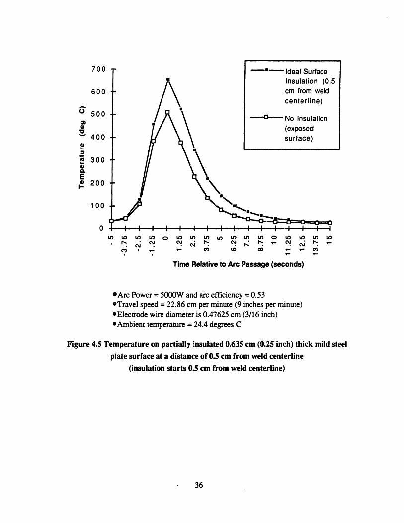
Comparison of figures 4.4 and 4.5 demonstrates the importance of placing surfaceinsulation close to the weld. The effects of moving insulation away from the weld are a
decrease in peak temperature and an increase in cooling rate. These are logical results
based on the form of the assumed relationship for convective heat loss (equation (4.14)).
Temperature differences between the plate surface and the surrounding water will be
largest close to the heat source. Therefore, convective heat losses will be greatest closerto the arc. Insulation placed close to the arc will thus be more effective in reducing
convective heat loss-and thereby increasing peak temperature and slowing the coolingrate-than insulation further from the arc.
Figure 4.6 (page 37) compares the effects of surface insulation with insulation
placed on the back of a quarter inch thick plate. For this thickness, convective heat loss
from the back of the plate is still significant, although far less important than convectivelosses from the surface.
/UU
600
500
400
! 300
E* 200
100
0C) e) I) O) W ) O V) O OIn OInn In 0 IO In In IU
Time Relative to Arc Passage (seconds)
*Arc Power = 5000W and arc efficiency = 0.53eTravel speed = 22.86 cm per minute (9 inches per minute)*Electrode wire diameter is 0.47625 cm (3/16 inch)*Ambient temperature = 24.4 degrees C
Figure 4.5 Temperature on partially insulated 0.635 cm (0.25 inch) thick mild steel
plate surface at a distance of 0.5 cm from weld centerline(insulation starts 0.5 cm from weld centerline)
5
IIf A A I
4A tU1 4VV
1200
1000
800
S600
E* 400I.-
200
0O U) LO) U) o U) 0 10 1 10 ) U) U) 0 10 1W W
* N- I C4J Cý - C r' : NP . C'J N-, .J , . . r,,
Time Relative to Arc Passage (seconds)
*Arc Power = 5000W and arc efficiency = 0.53*Travel speed = 22.86 cm per minute (9 inches per minute)*Electrode wire diameter is 0.47625 cm (3/16 inch)*Ambient temperature = 24.4 degrees C
Figure 4.6 Temperature on 0.635 cm (0.25 inch) thick mild steel plate surfaceat a distance of 0.5 cm from weld centerline
As plate thickness is increased, back side convective losses should decrease. When thesemi-infinite body thickness of approximately 0.75 inches is reached, there will be noconvection from the back of the plate according to the hypothesis of chapter 3. Thishypothesis is supported by the data presented in figure 4.7. Cooling rate and peaktemperature for a one-inch-thick plate are unaffected by the use of back side insulation.
LI)I.-
1-,.8--,- Irl" i jl " f " .
1 600 ---- Ideal SurfaceInsulation
1400 Adjacent To Weld
~3 1200 -- Ideal InsulationOn Back Of Plate
• 1000 ." 100 -- - No Insulation800
4 600
I- 400
200-
0 : t I t I JI I tI I I I I I 0 I IT· .0 ?
. .. I cV( ,,- ,.- CV0 I I1
Time Relative to Arc Passage (seconds)
*Arc Power = 5000W and arc efficiency = 0.53*Travel speed = 22.86 cm per minute (9 inches per minute)*Electrode wire diameter is 0.47625 (3/16 inch)*Ambient temperature = 24.4 degrees C
Figure 4.7 Temperature on 2.54 cm (1 inch) thick mild steel plate surfaceat a distance of 0.5 cm from weld centerline
Computational modeling has demonstrated that placement of surface insulation
close to the arc of a wet SMA weld could significantly increase the peak temperature anddecrease the cooling rate on the surface of the weld HAZ.
4.6 Modeling ConclusionsThe increase in peak temperature and the cooling rate reduction of a wet SMA
weld HAZ surface-demonstrated by the computational model-illustrate the potential of
the surface insulation method for improving wet weld quality. These changes in weld
cooling parameters could reduce the amount of martensite formed in wet weld HAZs,
lessen hydrogen embrittlement and oxygen and slag induced porosity, reduce residual
tensile stresses, and cause the formation of more concave weld beads.
In addition to demonstrating the potential of surface insulation, computationalresults have also shown a major limitation. Insulation must be placed close to the arc foroptimum results. Consequently, puddle manipulation will be limited, but moreimportantly, the insulation material will have to be capable of withstanding extremetemperatures. Appropriate insulation materials must maintain low conductivity and be
thermally stable at temperatures exceeding 1100 degrees C. Materials with suchproperties may not be readily available, or may be expensive or difficult to use (for
reasons such as low ductility).The computer model incorporated ideal insulation. Placement of actual insulation
materials on the surface of the model would have required reducing the number ofelements used in modeling the plate. Nekton is limited to 40 elements for 3-D models and40 elements were used in the plate model to obtain maximum accuracy. The result ofremoving plate elements to model insulation materials would have been a differentcooling curve in which the changes could not be attributed specifically to either theinsulation or the change in plate modeling parameters. Ideal insulation was thus usedbased on modeling considerations. With the exception of a perfect vacuum (which wouldbe impractical to create in the water) insulation with zero conductivity does not exist.(Even if material with zero conductivity could be acquired, the insulation to plate surfaceinterface would not be perfect and there would be heat transferred into the interface).Consequently, the computed results represent an upper bound of the effects of insulationmaterial. Actual insulation materials and imperfect interfaces encountered in practice willbe less effective in reducing weld quenching.
Modeling has demonstrated an insulation-induced reduction in surface HAZcooling. The surface is the area of the HAZ which is most rapidly cooled because ofdirect exposure to water. It is also the most likely location for crack initiation because ofseparation from the plate neutral axis and exposure to a corrosive environment. It isassumed that insulation will have less of an effect on the cooling rate of internal sectionsof the HAZ where quenching is not as severe.
Computational modeling has served to demonstrate the potential of surfaceinsulation. Laboratory tests must be conducted to prove its effectiveness.
CHAPTER 5. EXPERIMENTAL PROCEDURE
A series of experimental welds were made in the Welding Systems Laboratory ofMIT's Ocean Engineering Department to determine the effects of surface insulation onwet SMA welds. Welds were made manually with the base plates submerged in a smallreservoir filled with water and the welder standing outside the reservoir welding throughthe air-water interface. Surface hardness testing and microscopic weld examination wereused to evaluate the effects of insulation on the welds.
At the outset of the experimental phase of this research, attempts were made touse an automated welding system to make the experimental welds. It was thought that byusing an automated process, the parameters affecting heat input-such as arc size andtravel rate, weld current and voltage----could be held constant for all welds. Uninsulatedand fully insulated welds could then have been made with equivalent heat inputs, andsubsequently compared to evaluate the effect of insulation. This methodology could notbe used for two reasons. First, the only automated welding system which was availablefor experimental use was the laboratory Jetline Engineering GTAW system. Thisparticular system was designed to control the relatively low arc currents and voltages(i.e., 75 amps and 10 volts) used in GTA welding. The system was modified to weld witha SMAW electrode. However, testing demonstrated that the automation system could notconsistently control the arc currents and voltages required for wet SMA welding (150amps and 29 volts). Equivalent heat input profiles could not be obtained from one testweld to another. Second, the base plate travel (carriage) subassembly of the Jetline
Engineering system had too small a track width to move a water reservoir large enough
to maintain an approximately constant water temperature during welding. Ambient watertemperature increases of up to 20% were measured during automated welding trials witha reservoir small enough to be used with the Jetline Engineering system. An increase inambient water temperature during welding could reduce weld cooling rates. This effectwould never be present in the virtually infinite heat sinks (i.e., oceans and rivers) inwhich wet SMAW is actually performed. To accurately evaluate the effect of insulationunder actual welding conditions, ambient water temperature must be kept constant duringwelding. Consequently, a reservoir larger than that which could be moved by theautomated system had to be used. For these reasons it was decided early in theexperimental phase that welds would have to be made manually.
5.1 Description of the Experimental Procedure and EquipmentChanges in travel rate and arc length inherent in manual welding produce
variations in heat input. Thus--even with stringent control of other experimentalparameters---differences between uninsulated and fully insulated manual welds could notbe positively attributed to insulation, because differences could arise from varying heatinput profiles. Consequently, a procedure was developed that separated the effects ofvariations in heat input from insulation effects. Welds were insulated only along one sideand the remaining side was left uninsulated. Each weld, with it's specific heat input andinsulation configuration, could then be tested independently to evaluate the effects ofinsulation.
A welding jig was constructed that consisted of a base plate platform withsecuring clamps, electrode guides, insulation clamping screws, and a ground attachmentpoint. Base plates of varying thickness could be clamped into the jig. Insulation materialswere then clamped onto one side of the base plate with the edge of the insulation closestto the welding line positioned directly under the electrode guide so that all welds weremade with insulation adjacent to the weld line. (Control welds were made with noinsulation on either side of the base plate to establish baselines for the hardness testingphase of the experimental procedure). The welding jig and base plate were then placed ina reservoir containing 35.5 liters of fresh water, and the welding power supply groundwas attached to the jig/base plate assembly. Welds were made using the electrode guidesto ensure that the arc was directly adjacent to the insulation material during welding.Bead-on-plate welds were made because of the simplicity of this weld geometry. Figure6.1 shows a typical experimental set-up prior to placement of the jig in the weldingreservoir.
Figure 5.1 Welding Jig with Base Plate and Insulation
Three types of insulation were tested. All were fabrics woven from 3M NextelTM
312 alumina-boria-silica fibers. The primary difference between the fabrics that wereused was permeability. The Nextel fabrics were chosen because of their stability whenexposed to high temperatures (no shrinkage or strength loss after continuous exposure ofup to 1204 degrees C) and because of their low thermal conductivity (approximately 0.16W/m C at 650 degrees C) [13]. (In comparison, the thermal conductivity of fabrics wovenfrom asbestos (inorganic silica) fibers is approximately 0.17 W/m C at 650 degrees C[14].) High temperature stability allowed the insulation to be placed adjacent to the weldline, thereby optimizing it's effect on heat flow as discussed in section 4.5. Low thermalconductivity reduces through-insulation heat loss to the environment and is therefore ofprimary importance in reducing weld cooling rates. Additionally, the Nextel fabrics arepliable, can be formed to interface with any geometry, and are therefore practicalinsulating materials. Table 5.1 lists the properties of the three Nextel fabrics that weretested.
Table 5.1 Insulation Fabric Properties [13]
Fabric Style Thickness per Ply Weave Type Air Permeability (1)
(mm) mmin
AF-62 0.81 Double Layer 38
AF-40 1.27 5 Harness Satin 11.6
AB-22 (filter bag) 0.56 5 Harness Satin 5.3
(1) At constant pressure differential equal to 0.5 inches of water
A Miller Synchrowave 350 welding machine set for direct current straightpolarity was used as a power source. Welding current was 150 amps. Open circuit voltagewas 57.6 volts and average arc voltage during welding was 29 volts. All welding wasperformed with BROCO Softouch E70XX 1/8 inch diameter wet welding electrodes.
Temperature measurements were made in the welding reservoir immediatelybefore, during, and upon completion of welding. Measurements were made at twopositions, one at the edge of the plate being welded, and the other at a location in thereservoir removed from the welding site. K-type thermocouples (with a temperaturemeasurement range of -200 to 1370 deg. C) connected to a calibrated OMEGA RD-103-
AR chart recorder were used to make the temperature measurements. All welds were
timed, and bead length and average bead width recorded. Experimental weld parameters
are presented in table 5.2.
Table 5.2 Experimental Weld Parameters (1)
Weld Bead Travel Base Reservoir Reservoir InsulationNo. Lgth/Avg Rate Metal Temp. Temp. (8 plys
Bead (cm/s) (2) Prior to Increase applied to 1Width Welding During side of weldcm/cm (deg. C) Welding for MS, 4
(deg. C) plys to(3) both sides
for HTS)
Control 1 13.2/0.5 0.73 MS 22.9 0.1 N/A
MS 1 12.5/0.5 0.65 MS 22.9 0.2 AF-40
MS2 9.2/0.5 0.56 MS 21.3 0.0 AF-40
MS3 12.7/0.5 0.74 MS 15.3 0.0 AF-40
MS4 13.0/0.5 0.74 MS 18.6 0.2 AF-40
MS5 13.2/0.5 0.73 MS 20.7 0.1 AF-40
Control 2 12.0/0.4 0.71 HTS 23.9 0.1 N/A
HTS 1 13.0/0.4 0.72 HTS 24.0 0.1 AB-22
(1) All welds made with BROCO Softouch E70XX 1/8 inch diameter wet weldingelectrodes with 150 amp welding current and 29 volt average arc voltage. Base platedimensions were 6 inches in the direction of the weld line and 4 inches perpendicularto the weld for MS, and 5.5 and 8 inches respectively for HTS.
(2) CE of MS (ASTM A36 mild steel) = 0.285 and CE of HTS (DH-36 High TensileStrength Steel) = 0.41. Base plate thicknesses were 0.25 inch for MS and 0.5 inch forHTS.
(3) From average of temperatures at both thermocouple locations
5.2 Evaluation of Experimental WeldsAccording to Okumura and Yurioka of the Nippon Steel Corporation, "The
hardness of heat affected zones is the most basic property in assessing the weldability ofsteels" and, "HAZ hardness tests are generally conducted as one of the welding procedureapproval tests" [15]. As discussed in section 2.1 of this thesis, HAZ hardness is directlyrelated to the weld cooling rate. MIT welding engineering professor K. Masubuchi hasstated that hardness testing is a more reliable method of determining the effects of various
weld parameters on the cooling rate than direct temperature measurement, because of the
difficulty of obtaining accurate temperature readings close to a welding arc.
Consequently, the primary means used in this experiment to evaluate the effects of
surface insulation on weld cooling rates was HAZ hardness testing. Hardness was
measured on all mild steel welds with an Acco Wilson Model 4JR Rockwell Hardness
Tester. Welds were not ground prior to hardness testing because grinding heat input
would have had a non-measurable effect on surface hardness. In addition to hardness
testing, the HTS welds, and one mild steel weld were sectioned, polished, acid etched,
and visually inspected using a Hirox Co. LTD. Model KN-2200 MD2 fiber optic
microscope.
CHAPTER 6. EXPERIMENTAL RESULTS
More than fifty trial welds were made on mild steel plates during the initial phase
of the manual welding experiment. The purpose of these welds was to practice thewelding technique so that welds with relatively consistent travel rate and bead profilecould be attained. At first, the majority of the welds had longitudinally varying beadprofiles. Four of these trial welds (two of which had been insulated with AF-62 fabric andtwo with AF-40) were tested for hardness. The standard deviations of the hardness valueswere high because of bead profile irregularities. However, the results did indicate that theless permeable AF-40 fabric provided better insulation than AF-62. This result is
intuitive. The purposes of insulation are to provide a thermal resistance and to displacewater from the plate surface so as to limit convective heat losses. The less permeableinsulation was more effective in displacing water from the plate surface, limitingconvection, and thereby reducing the weld cooling rate. Consequently, welds made withAF-40 insulation showed a slight statistically relevant reduction in surface hardness ascompared to the welds insulated with AF-62. Because of bead irregularities, measuredhardness values for these welds were considered unsuitable for use as experimental data.However, the conclusion that AF-40 was a more effective insulating material than AF-62was assumed to be valid, and further tests were performed solely with the less permeableAF-40 and AB-22 materials. (AB-22 became available after mild steel welding had beencompleted, and was therefore used only in the subsequent HTS phase of the experiment).
The Nextel fabrics proved to be quite durable. They were capable of being usedrepeatedly, and even when subjected directly to the submerged arc, they did not melt.
With practice, welding travel rate and weld bead profile consistency wereattained. Eight "experimental" welds were then made. Six were made on 0.25 inch thick0.285 CE mild steel plate. These mild steel welds consisted of one control weld, whichwas not insulated, and five welds that were insulated on one side of the weld line. After
completion of the mild steel testing phase, two experimental welds were made on 0.5
inch thick 0.41 CE HTS. This grade of steel was chosen because recent tests conducted
by the Naval Sea Systems Command had found underbead cracking in all wet weldsmade on plates with CEs greater than 0.40. Welding parameters for all experimentalwelds were presented previously in table 5.2. A photographs of two typical experimentalmild steel welds is shown in figure 6.1.
Figure 6.1 Photographs of Typical Experimental Mild Steel Welds
6.1 Results From Hardness Testing and Visual Inspection of Welds Made on
Mild Steel Plates
Hardness testing results from the mild steel plate welds are presented in tables 6.1
through 6.3. In each case, ten hardness readings were taken on each side of the weld line.
The weld crown was used as a lateral reference because of the relative ease of identifying
the apex of the crown. (The exact location of the weld toe would have been more difficult
46
Table 6.1 Hardness Testing Results from Mild Steel Control Weld and MS1
Control
Rockwell A Hardness(1/4 inch from weld crown) X2 ((Sample Mean-Sample Value) 2)
Xu (Smpl Mean) Xi (Smpl Mean) su (Smpl Std Dev) s, (Smpl Std Dev)45.45 42.70 2.29 2.63
U t t(0.60) t(0.70)2.60 0.47 0.26 0.54
MS 5
Rockwell A Hardness(1/4 inch from weld crown) X2 ((Sample Mean-Sample Value) 2 )
Sample Uninsulated Side insulated Side Uninsulated Side Insulated Side
46.049.046.548.050.043.546.045.045.544.0
34.038.541.044.545.035.041.543.535.038.0
0.127.020.022.72
13.328.120.121.820.725.52
31.361.211.96
24.0129.1621.163.61
15.2121.162.56
(Smpl Mean)46.35
Xi (Smpl Mean) su (Smpl Std Dev)39.60 1.99
st (Smpl Std Dev)3.89
t t(0.80) t(0.90)0.93 0.88 1.38
a
3.26
to specify). Hardness was measured at a lateral offset of 1/4 inch from the weld crown
because this was the closest that the weld could be approached with the indenter tip of thetesting device without the indenter bale impacting the weld bead reinforcement. Fromvisual inspection it appeared that measurements taken at the 1/4 inch offset distance werewithin the weld HAZ. Hardness readings were taken in pairs (one reading on theinsulated side and one on the uninsulated side) at random locations along the weld. The
Rockwell A testing scale was chosen because it provided readings close to 50% scale
deflection for the samples being evaluated.
To determine the statistical significance of the results the "Student's t" analysiswas used. This analysis is valid for sample sizes of less than 30 with an assumed normaldistribution [16]. The t analysis is described in the following paragraphs .
First, the sample mean (X) from each population (i.e., uninsulated side orinsulated side) is computed. Second, the sample standard deviation (s) is computed for
each population. The statistic a is then calculated as shown in equation (6.1).
NCsy + Ns2 (6.1)N, + N2 -2
Where:NI, N2 are the number of samples taken in populations 1 and 2s1, s2 are the sample standard deviations of populations 1 and 2
Finally, the statistic t is computed using equation (6.2).
X, -Xt = (6.2)a 1/N+1/N 2 6.2)
The t statistic represents the significance level of the difference in the samplemeans of the two populations. Hence, a high value of t (a high significance level)indicates that there is a high probability that a difference in sample means is the result ofsampling from two physically distinct populations (i.e., a brittle uninsulated side and aductile insulated side). A low value of t (low significance level) is indicative of thesamples having been drawn from the same overall population, with any difference insample means being the result of measurement standard deviations. The latter case wouldbe expected for control welds since no physical difference should exist in the hardnessvalues measured on either side of these welds. Significance levels (i.e., t(O.90), t(0.80))
are tabulated for different degrees of freedom. (The number of degrees of freedom of astatistic is defined as the sample size minus the number of population parameters which
must be estimated from sample populations. In the case of t, the number of degrees offreedom = N-l, where N is the sample size [16]). It is these significance levels which aretabulated-along with the computed values of t-in tables 6.1 through 6.3.
The results of control weld testing presented in table 6.1 demonstrate that there isapproximately a 10% measurement error inherent in the experimental and testingprocedures and sample sizes (N = 10) that were used. (t = t(0.60), signifying a 60%significance level for the difference in mean sample hardness values between sides I and2. Since this is a control weld, we would expect t = t(0.50), a 50% or randomsignificance level. Thus the measurement error can be approximated as the differencebetween these significance levels which is 10%). The primary methods for reducingmeasurement error are to reduce sample standard deviation (a) and increase samplesize.(N) The standard error associated with a sample mean (u') is given by equation
(6.3) [16].
ox = - (6.3)
Sample standard deviation values were inherent to the manual welding process and couldnot be reduced without improving the consistency of heat input along the length of theweld. Additionally, since To is proportional to the inverse square root of the sample size,
a sample size of N = 100 would theoretically have been required to reduce themeasurement error from 10% to approximately 3-4%. Sample sizes of 100 would nothave been practical given the lengths of the welds being tested. Consequently, 10%measurement errors are associated with all hardness values reported in this thesis.
The data presented in tables 6.1 through 6.3 shows that all five insulated mildsteel welds demonstrated decreased surface HAZ hardness on the insulated sides of theweld beads. Furthermore, in addition to this insulation effect being demonstrated in allfive welds, the results are statistically significant even after measurement error has beenconsidered. Specifically, the average significance level for the reduction in surfacehardness due to insulation in welds MS 1 through MS5 is t(0.77). This is 17% higher thanthe significance level of the control weld. Figures 6.2 and 6.3 graphically depict themeasured mean hardness differences between insulated and uninsulated sides of all mild
steel welds, and the absolute relevant hardness differences between sides for welds MS 1through MS5, respectively.
50454035302520151050
-6 T- Cl) ) UC Cl1CO C
0
Figure 6.2 Comparison of Mean Hardness Values for Mild Steel Test Welds
5-
4.
MS1 MS2 MS3 MS4 MS5
* 1((Uninsulated Side Sample Mean Hardness)-(Insulated Side Sample Mean Hardness))-(Hardness Difference Between Control Weld Sides 1 and 2)1
Figure 6.3 Experimentally Relevant Higher Mean Hardness Values of the
Uninsulated Sides of Mild Steel Welds 1 through 5
M Uninsulated Side (side 1of control weld)
O Insulated Side (side 2 ofcontrol weld)
+
---
It is important to note that one-sided surface insulation would theoretically be lesseffective in reducing weld cooling rates-and surface HAZ hardness-than two sided orfull insulation, because of asymmetric heat flow in the former. The weld centerline is nota symmetry plane, and greater heat flux through the less thermally resistant uninsulatedside would be expected. The result would be a faster overall cooling rate for a weldinsulated on one side than for a fully insulated weld.
Visaal inspection of the sectioned mild steel weld (MS 5) was inconclusive. Nodifference in HAZ shape between the insulated and uninsulated sides was evident at amagnification level of 10 X.
6.2 Results From Visual Inspection of Welds Made on High Strength Steel PlatesMicroscopic examination of the two 0.41 CE HTS welds revealed differences in
the fusion line between the uninsulated and fully insulated welds. At 10 X magnificationthe uninsulated weld fusion line was traversed by numerous perpendicular underbeadcracks. The fusion line of the insulated weld was smooth, and underbead cracks were notapparent. This observation was confirmed by an AWS certified welding inspector, Mr.Robert Murray of the Naval Sea Systems Command. Mr Murray stated that in previouswet welding tests of plates exceeding 0.40 CE, underbead cracking had been found in allwelds. This form of cracking can be attributed to rapid contraction of the HAZ as a resaltof weld quenching.
No definitive conclusions can be made from the examination of two welds.However the results of visual examination of the HTS welds, coupled with the hardnesstesting results from the mild steel welds, suggest that surface thermal insulation mayindeed slow the cooling rates of wet SMA welds as predicted by computational modeling.Further, more controlled testing is required to definitively prove this hypothesis, and toaccurately quantify the effect of insulation-induced quenching reduction on weld ductilityand strength.
CHAPTER 7. CONCLUSION
This thesis has demonstrated both computationally and experimentally thatthermal insulation can be used to reduce the quenching rate and thereby improve thequality of wet SMA welds. Thermal insulation has been shown to be practically and
economically feasible. Placement of static insulation during fit-up will have only amarginal impact on weld set-up times. Commercially available, pliable, re-usable, non-toxic, and relatively inexpensive insulation materials (Nextel AB-22 fabric is sold aswoven seamless tubing with a 4 5/8 inch outside diameter at a cost of $40.40 per linear
foot) have been tested in the laboratory with satisfactory results. However, because of
limitations in experimental capabilities (specifically the use of the author, a non-coded
welder, to make manual experimental welds) the full potential of this technology advance
has not been demonstrated.As a result of this initial research, the U.S. Navy has initiated a program to
evaluate more thoroughly the effect of insulation on wet SMA welds. The Navy plans touse AWS coded wet welders/divers to perform butt welds while fully submerged in a
large testing tank. These welders will weld at pre-specified travel rates with tightlycontrolled welding parameters. Heat input consistency between welds will allow testing
and comparison of both fully insulated (insulation on both sides of the joint) and
uninsulated joints. Welds will be destructively bend-tested to directly measure ductilityand strength. Additionally, research will be performed to determine if better insulationmaterials than the Nextel fabrics-lower conductivity and permeability, and improvedthermal stability and pliability-are commercially available. All research and testing will
be carried out under the provisions of the Massachusetts Institute of Technology,Technology Licensing Office, through which a patent application has been filed with the
U.S. Patent Office (case number 6107) entitled "Thermal Insulation of Wet ShieldedMetal Arc Welds."
Results from the Navy testing program could convincingly demonstrate the
viability of thermally insulated wet welds, thereby leading to improvements in wet SMA
weld quality, and allowing wet SMAW to be used on a wider range of materials in bothcommercial and military applications.
REFERENCE LIST
1. American Welding Society. Specification for Underwater Welding. AWS. Miami.1982.
2. Tsai, C.L. Parameteric Study on Cooling Phenomena in Underwater Welding.Massachusetts Institute of Technology. 1977.
3. Masubuchi, K., and D.C. Martin. Mechanisms of Cracking in HY-80 SteelWeldments. Welding Journal Research Supplement. August 1962.
4. Masubuchi, K., et al. TMCP Steels for Construction and Repair of Marine Structures.1992.
5. ARCAIR CO. ARCAIR Instruction Manual for Underwater Cutting and Welding.1982.
6. West, T.C., G. Mitchell, and E. Lindberg. Wet Welding Evaluation for Ship Repair.Welding Journal, August 1990: 46-56.
7. Masubuchi, K., A.B Gaudiano and T.J. Reynolds. Technologies and Practices ofUnderwater Welding. Underwater Welding Conference Proceedings, 1983: 49-70.
8. Stalker, A.W. Welding Institute Research on Underwater Welding. UnderwaterWelding for Offshore Installations. The Welding Institute. Abington Hall. 1977.
9. Bouaman, H., and J. Haverhals. Underwater Welding With Covered Electrodes.Lastechbik, 1971: Vol. 37, No. 12, 219-226.
10. Tsai, C.L. et al. Development of New Improved Techniques for Underwater Welding.MIT Sea Grant Program. 1977: MITSG 77-9.
11. Satoh, K. et al. Study on Improvement of Locally Drying Underwater Welding Jointby Retarded Cooling Method. Journal of the Japanese Welding Society, August 1982:665-672.
12. Zienkiewicz, O.C., The Finite Element Method in Structural and ContinuumMechanics. McGraw Hill. London. 1968.
4 Lines of passive scalar data follow2 CONDUCT; 2RHOCP1.00000 1.00000 1.00000 1.00000 1.00000
1.000001.000001.00000
1.00000 1.000001.00000 1.000001.00000 1.00000
1.000001.000001.00000
1.00000
13 LOGICAL SWITCHES FOLLOWF IFFLOW
T IFHEATT IFTRANF F F F F F F F F F F IFNAV & IFADVC (convection in P.S. fields)F F T T T T T T T T T T IFTMSH (IF mesh for this field is T mesh)F IFAXISF IFSTRSF IFSPLITF IFMGRIDF IFMODELF IFKEPSF IFMVBDF IFCHAR0.119063 0.119063 -0.357188E-01 -0.178594E-01 XFAC,YFAC,XZERO,YZERO**MESH DATA** 6 lines are X,Y,Z;X,Y,Z. Columns corners 1-4;5-840 3 40 NEL, NDIM, NELV
FORTRAN code used to establish model boundary conditions(NEKTON. user File).
C USER SPECIFIED SUBROUTINES:C - boundary conditionsC - initial conditionsC - variable propertiesC - forcing function for fluid (f)C - forcing function for passive scalar (q)C - general purpose routine for checking errors etc.