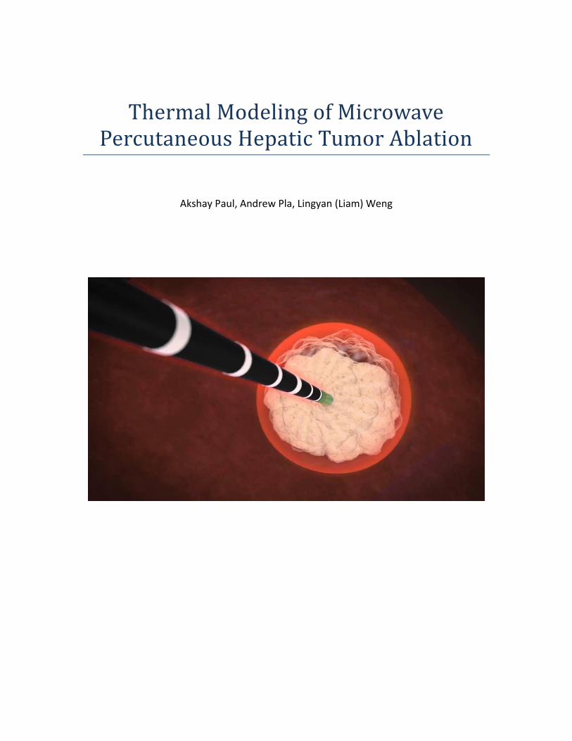
Thermal Modeling of Microwave Percutaneous Hepatic Tumor Ablation

Akshay Paul, Andrew Pla, Lingyan (Liam) Weng

2

1. Background and Introduction

Thermal ablation is widely accepted as a method of treatment for certain benign or

malignant tumors in the kidneys, liver, and bones [1, 2]. The most prevalent forms of

thermal ablation include radiofrequency ablation (RFA) and microwave ablation (MWA),

owing to their ability to generate heat in the tissue and raise the tissue temperature to

the lethal point, 50-60 °C [2]. This temperature range is known to induce coagulation

necrosis, i.e. cell death. The principle mechanisms behind RFA and MWA are the Joule

effect and dielectric heating, respectively [2]. Briefly, according to the Joule effect, or

Joule’s first law, RF current causes resistive heat in the electric conductive tissue,

whereas MWA introduces electromagnetic field to create molecular motions,

generating heat due to the dielectric property of the tissue [2]. MWA is shown to be

more promising in treating tumors, especially for those who have a tumor diameter

greater than 3 cm and for tissues that have high impedance which prevents RF current

flow, because of its capability to rapidly generate heat and to ignore tissue impedance

[1, 2, 3].

A typical percutaneous surgical procedure for MWA involves insertion of an antenna,

which acts as the applicator, into the tumor area with image guidance. A power

generator supplies a power of around 0-300W depending on the number of antennae

employed and the frequency used [1, 2, 3]. Specifically, there are three types of MWA: i)

First generation without a coupled cooling system; ii) Second generation with a coupled

cooling system but limited magnitude of power; iii) Third generation with both cooling

and high power generation abilities [1]. The temperature profile, or the ablation zone, is

primarily influenced by the tissue properties and the microwave interaction with the

tissue [3].

2. Problem Statement

Hepatic tumors are a common target of MWA, and a theoretical model could enable us

to gain an insight into the heat transfer behavior to further study the relationship

between propagation of the electromagnetic wave and heat transfer in the liver tissue

[3]. The aim of this project is to model a 1-Dimensional temperature profile within

hepatic tumor tissue from the tip of the applicator to 1 cm beneath the tissue to justify

the aforementioned heat conduction and ablation efficiency with respect to time and

space with given tissue properties, ablation system properties, an initial condition, and

boundary conditions.

3

3. Relevant Mathematical Background

Microwave ablation is an attractive technology for clinical application because of fast

and high heat delivery to target tissue and, in some cases, no contact requirement.

Microwave generators deliver electromagnetic energy to target tissues through an

antenna probe at frequencies of 915 Mhz or 2.45 Ghz. These high electromagnetic

frequencies induce rotation of molecules, such as water and proteins, rapidly generating

heat in tissue. This process is called dielectric heating and is the fundamental

transformation of energy in this system [3,4,6].

For the effective treatment of clinically observed liver tumors, the microwave ablation

device must create a uniform heating area that can extend past the boundaries of the

malignancy [3].

In this report, the goal is to model the temperature of tissue in a region-of-interest

undergoing microwave ablation. A faithful representation of this medical treatment will

describe the interaction of electromagnetic energy with liver tissue and the diffusion of

delivered-heat through targeted tissue.

Microwave energy is characterized by Maxwell’s equations [3].

∇ ∙ 𝑫 = 𝜌𝑓𝑟𝑒𝑒

∇ ∙ 𝑩 = 0

∇ × 𝑬 = −𝜕𝑩

𝜕𝑡

∇ × 𝑯 = 𝑱 +𝜕𝑫

𝜕𝑡

D [C/m2] electric flux density

B [T] magnetic field

E [V/m] electric field strength

H [A/m] magnetic field intensity

𝜌𝑓𝑟𝑒𝑒 [C/m2] free charge density

J [A/m2] current density

4

The Maxwell equations can then be solved to determine the propagation of

electromagnetic energy through a region of interest. The interactions of these

electromagnetic fields with biological tissue can then be characterized using tissue

properties such as density, specific heat, permittivity, and conductivity [6]. Materials

that do not effectively absorb electromagnetic energy are referred to as low-loss,

whereas other materials may exhibit high absorption of electromagnetic energy. This

absorptivity can be defined as the material’s conductivity, σ, divided angular frequency,

ω, and dielectric permittivity, ε [3,4].

𝜀𝑟 = 𝜀′𝑟 −𝑗𝜎

𝜔𝜀0

Since most biological tissue is highly absorbing of propagating electromagnetic energy,

its permittivity can be described with consideration of the electromagnetic frequency.

The Cole-Cole model describes tissue permittivity as a function of frequency and tissue

property constants [3].

𝜀(𝑓) = 𝜀∞ −𝛴(𝜀𝑠 − 𝜀∞)

1 + (𝑗2𝜋𝑓𝜏𝑛).1−𝛼𝑛

+𝜎𝑖2𝜋𝜀0

𝜀∞ permittivity at infinite frequency

𝜀𝑠 permittivity at dc

f frequency

𝜏𝑛 relaxation time constant

α attenuation constant

𝜎𝑖 [S/m] dc conductivity

The conductivity and permittivity of tissue, like most biological systems, is dependent

upon temperature itself. Temperature dependence of tissue dielectric properties arises

primarily from the significant water concentration in organ tissue [3,6]. As microwave

ablation heats an area of tissue, water molecules evaporate and rising temperatures

irreversibly change protein structures, causing the conductivity and permittivity of the

tissue to change [4].

5

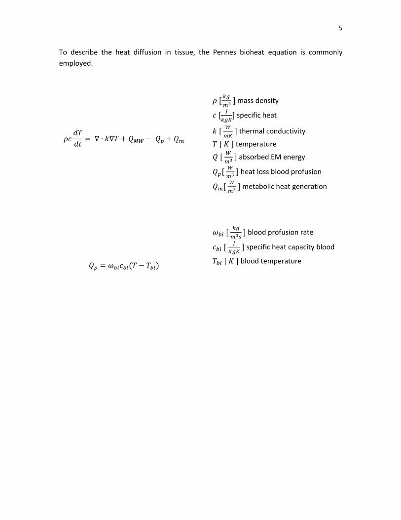
To describe the heat diffusion in tissue, the Pennes bioheat equation is commonly

employed.

𝜌𝑐𝑑𝑇

𝑑𝑡= ∇ ∙ 𝑘∇𝑇 + 𝑄𝑀𝑊 − 𝑄𝑝 + 𝑄𝑚

𝜌 [𝑘𝑔

𝑚3 ] mass density

𝑐 [𝐽

𝑘𝑔𝐾] specific heat

𝑘 [ 𝑊

𝑚𝐾 ] thermal conductivity

𝑇 [ 𝐾 ] temperature

𝑄 [ 𝑊

𝑚3 ] absorbed EM energy

𝑄𝑝[ 𝑊

𝑚3 ] heat loss blood profusion

𝑄𝑚[ 𝑊

𝑚3 ] metabolic heat generation

𝑄𝑝 = 𝜔𝑏𝑙𝑐𝑏𝑙(𝑇 − 𝑇𝑏𝑙)

𝜔𝑏𝑙 [ 𝑘𝑔

𝑚3𝑠 ] blood profusion rate

𝑐𝑏𝑙 [ 𝐽

𝐾𝑔𝐾 ] specific heat capacity blood

𝑇𝑏𝑙 [ 𝐾 ] blood temperature

6

The heat source component QMW is generated in tissue by the electromagnetic energy

absorption. This equation is called the specific absorption rate, SAR and describes the

microwave heat source term in this system as a function of conductivity and electric field [3].

𝑄 =1

2𝜎|𝐸|2

Now that the overall heat equation is defined and so is the thermal conductivity of tissue with

respect to temperature, the focus can shift to the final piece of the SAR equation – the electric

field component. This report has previously discussed how microwave dynamics can be

described in terms of an electric field using the Maxwell equations. Therefore, to begin

derivation of an electric field equation that is representative of microwave energy in this

system, one can examine device constants.

A typical clinical microwave ablation device operates with 100 Watts of power at a frequency of

2.4 GHz.

𝑃 = 𝐼 ∗ 𝑉 [𝑊𝑎𝑡𝑡𝑠 =𝐽𝑜𝑢𝑙𝑒𝑠

𝑠𝑒𝑐]

𝑓 = 2.4 𝐺𝐻𝑧 𝜔 = 2𝜋𝑓

From the power formula, current can be defined in terms of power and voltage. The current

can then be substituted into the charge equation, q:

𝑞 = 𝐼 ∗ 𝑡 = 𝐼𝑚 sin(𝜔𝑡) ∗ 𝑡

𝑞 =𝑃

𝑉𝑚 sin(𝜔𝑡)𝑡 =

𝜀0𝐴

2𝑑𝑉𝑚 sin(𝜔𝑡)

Charge q is now defined in terms of voltage and frequency. It can now be input into the electric

field equation for a conducting sphere:

𝐸 = 𝑞

4𝜋𝜀0𝑟2 [

𝑉𝑜𝑙𝑡𝑠

𝑚]

Substitution of the q term into the spherical conductor equation produces an electric field

equation that is dependent on source voltage, frequency, and distance from source [3,4,6].

𝐸 = 𝑉𝑚 sin(𝜔𝑡)𝑑

2𝑟2 [

𝑉𝑜𝑙𝑡𝑠

𝑚]

Considering that the final electric field equation for this microwave generator is dependent on

voltage, one can work in reverse and solve for the electric field in terms of power.

𝐸2 =𝑃

𝐴𝜀0𝑑𝑡

7

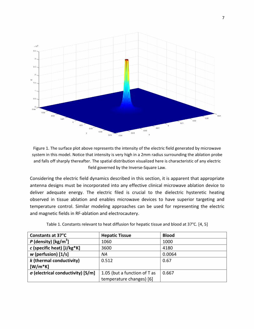
Figure 1. The surface plot above represents the intensity of the electric field generated by microwave

system in this model. Notice that intensity is very high in a 2mm radius surrounding the ablation probe

and falls off sharply thereafter. The spatial distribution visualized here is characteristic of any electric

field governed by the Inverse-Square Law.

Considering the electric field dynamics described in this section, it is apparent that appropriate

antenna designs must be incorporated into any effective clinical microwave ablation device to

deliver adequate energy. The electric filed is crucial to the dielectric hysteretic heating

observed in tissue ablation and enables microwave devices to have superior targeting and

temperature control. Similar modeling approaches can be used for representing the electric

and magnetic fields in RF-ablation and electrocautery.

Table 1. Constants relevant to heat diffusion for hepatic tissue and blood at 37°C. [4, 5]

Constants at 37°C Hepatic Tissue Blood

Ρ (density) [kg/m3] 1060 1000

c (specific heat) [J/kg*K] 3600 4180

w (perfusion) [1/s] NA 0.0064

k (thermal conductivity) [W/m*K]

0.512 0.67

σ (electrical conductivity) [S/m] 1.05 (but a function of T as temperature changes) [6]

0.667

8

4. Mathematical Solution

4.1 Simplified Equation Solution

Initially, an analytical solution to the full bio-heat equation was attempted. The solution that

was arrived at and presented, however, was later realized to not be accurate. The nature of the

full bio-heat equation makes an analytical solution prohibitively difficult to attain. With this in

mind, a simplified version of the system was formulated.

In this simplified system, the heat provided by the microwave antenna is not represented by a

source term, but by a constant boundary temperature, TM. Many ablation systems regulate the

temperature of the antenna to a constant level, so this is a reasonable assumption [1]. A further

simplification of this model is that temperature change due to perfusion is also ignored. This

should be kept in mind when viewing the results, as perfusion would normally be pushing the

overall temperature of the system towards normal body temperature, To. As a result of these

simplifications, the equation that we set out to solve analytically was the following:

𝜕𝑇

𝜕𝑡= 𝐷

𝜕2𝑇

𝜕𝑥2 With Initial and Boundary conditions: {

𝑇(𝑥, 0) = 𝑇𝑜𝑇(0, 𝑡) = 𝑇𝑀𝑇(𝐿, 𝑡) = 𝑇𝑜

, and 𝐷 = 𝑘

𝜌𝐿𝑐𝐿

where D is a constant determined by k, the heat diffusion coefficient; ρL, the density of liver

tissue; and cL, the specific heat of liver tissue. The initial condition sets the system at regular

body temperature, To=37°C. The left boundary condition is TM =100°C, as discussed above, and

the right boundary condition is the end of the ablation zone, assumed to be a blood vessel,

which provides a constant heat value of To. A length L of 4 cm is used, which corresponds to a

3cm tumor radius + 1cm buffer zone.

This is a standard heat equation with inhomogeneous boundary conditions. It was solved using

the poison tooth extraction method. A homogeneous solution and a particular solution were

found and added together to determine the full form of the solution to the equation. Once this

was done, the constant An was found to complete the solution.

The first step was the homogeneous solution with boundary conditions equal to zero. This is

solved for through the separation of variables method. This process is shown below.

Step 1, substitute the temperature function for two single-variable functions and rearrange:

𝑇(𝑥, 𝑡) = 𝜙(𝑥)𝐺(𝑡)

𝜙(𝑥)𝜕𝐺(𝑡)

𝜕𝑡= 𝐷

𝜕2𝜙(𝑥)

𝜕𝑥2𝐺(𝑡)

9

𝜕𝐺(𝑡)𝜕𝑡𝐺(𝑡)

∗1

𝐷=

𝜕2𝜙(𝑥)𝜕𝑥2

𝜙(𝑥)= −𝜆

One half of this equation is dependent solely on t, while the other is dependent solely on x.

Because the two halves are equal but dependent on different variables, they must both be

equal to a constant, given by –λ.

Step 2, split the equation into two ODE halves and solve each independently.

Step 2.1, solving the time-dependent equation:

𝜕𝐺(𝑡)𝜕𝑡𝐺(𝑡)

∗1

𝐷= −𝜆

𝜕𝐺(𝑡)

𝜕𝑡+ 𝜆𝐷𝐺(𝑡) = 0

𝐺(𝑡) = 𝑒−𝜆𝐷𝑡

Step 2.2, solving the space-dependent equation:

𝜕2𝜙(𝑥)𝜕𝑥2

𝜙(𝑥)= −𝜆

𝜕2𝜙(𝑥)

𝜕𝑥2+ 𝜆𝜙(𝑥) = 0

𝜙(𝑥) = 𝐴𝑐𝑜𝑠(√𝜆𝑥) + 𝐵𝑠𝑖𝑛(√𝜆𝑥)

Step 3, substitute in the zero value boundary conditions to find λ:

𝜙(0) = 0 = 𝐴𝑠𝑖𝑛(0) + 𝐵𝑐𝑜𝑠(0)

0 = 𝐵

𝜙(𝐿) = 0 = 𝐴𝑠𝑖𝑛(√𝜆𝐿)

√𝜆𝐿 = 𝑛𝜋 Where 𝑛 = 1, 2, 3, …

𝜆 = (𝑛𝜋

𝐿)2

𝜙(𝑥) = 𝐴𝑛 sin (𝑛𝜋

𝐿𝑥)

10

Step 4, recombine the two halves of equation and take their linear combination by the

superposition principle for the homogeneous solution, TH(x,t):

𝑇𝐻(𝑥, 𝑡) = 𝜙(𝑥)𝐺(𝑡) = ∑𝐴𝑛 sin (𝑛𝜋

𝐿𝑥) 𝑒−(

𝑛𝜋𝐿)2𝐷𝑡

∞

𝑛=1

With the homogeneous solution obtained, the next step is to solve for the particular solution.

This is done by assuming steady state conditions and the original boundary conditions.

Step 5, determine the equation at steady state:

𝜕𝑇

𝜕𝑡= 0 (Steady state condition)

0 = 𝐷𝜕2𝑇

𝜕𝑥2 With initial and boundary conditions: {

𝑇(𝑥, 0) = 𝑇𝑜𝑇(0, 𝑡) = 𝑇𝑀𝑇(𝐿, 𝑡) = 𝑇𝑜

Step 6, solve for TP(x):

𝑇𝑃(𝑥) = ∫∫0 𝑑𝑥 𝑑𝑥 = 𝑐1𝑥 + 𝑐2

𝑇𝑃(0) = 𝑇𝑀 = 𝑐1(0) + 𝑐2

𝑐2 = 𝑇𝑀

𝑇𝑃(𝐿) = 𝑇𝑜 = 𝑐1(𝐿) + 𝑇𝑀

𝑐1 =𝑇𝑜 − 𝑇𝑀

𝐿

𝑇𝑃(𝑥) =𝑇𝑜 − 𝑇𝑀

𝐿𝑥 + 𝑇𝑀

Step 7, combine the particular and homogeneous solutions for the full solution:

𝑇(𝑥, 𝑡) =𝑇𝑜 − 𝑇𝑀

𝐿𝑥 + 𝑇𝑀 +∑𝐴𝑛 sin (

𝑛𝜋

𝐿𝑥) 𝑒−(

𝑛𝜋𝐿)2𝐷𝑡

∞

𝑛=1

Step 8, solve for the constant An using the equation for An

𝐴𝑛 =2

𝐿∫ (𝑢(𝑥, 0) − 𝑇𝑃(𝑥)) sin (

𝑛𝜋𝑥

𝐿) 𝑑𝑥

𝐿

0

11

𝐴𝑛 =2

𝐿∫ (𝑇𝑜 −

𝑇𝑜 − 𝑇𝑀𝐿

𝑥 − 𝑇𝑀) sin (𝑛𝜋𝑥

𝐿) 𝑑𝑥

𝐿

0

𝐴𝑛 = ∫ (𝑇𝑜 − 𝑇𝑀) sin (𝑛𝜋𝑥

𝐿) 𝑑𝑥 +

2

𝐿∫ (

𝑇𝑜 − 𝑇𝑀𝐿

𝑥) sin (𝑛𝜋𝑥

𝐿) 𝑑𝑥

𝐿

0

𝐿

0

Here the integral is split into two parts. The first integral is simpler and will be solved first. The

second integral requires integration by parts and will be solved afterwards.

Step 8.1, solve the first integral:

2

𝐿∫ (𝑇𝑜 − 𝑇𝑀) sin (

𝑛𝜋𝑥

𝐿) 𝑑𝑥

𝐿

0

=2(𝑇𝑜 − 𝑇𝑀)

𝐿∫ sin (

𝑛𝜋𝑥

𝐿)𝑑𝑥

𝐿

0

=2(𝑇𝑜 − 𝑇𝑀)

𝐿

−𝐿

𝑛𝜋(cos(𝑛𝜋) − cos(0)) =

−2(𝑇𝑜 − 𝑇𝑀)

𝑛𝜋((−1)𝑛 − 1)

Step 8.2, solve the second integral using integration by parts:

2

𝐿∫ (

𝑇𝑜 − 𝑇𝑀𝐿

𝑥) sin (𝑛𝜋𝑥

𝐿) 𝑑𝑥 =

2(𝑇𝑜 − 𝑇𝑀)

𝐿2∫ 𝑥𝑠𝑖𝑛 (

𝑛𝜋𝑥

𝐿) 𝑑𝑥

𝐿

0

𝐿

0

𝑢 = 𝑥 𝑑𝑣 = sin (𝑛𝜋𝑥

𝐿)𝑑𝑥

𝑑𝑢 = 𝑑𝑥 𝑣 = −cos (𝑛𝜋𝑥

𝐿) 𝐿

𝑛𝜋

2(𝑇𝑜 − 𝑇𝑚)

𝐿2[−𝑥𝑐𝑜𝑠 (

𝑛𝜋𝑥

𝐿)𝐿

𝑛𝜋− ∫ −cos (

𝑛𝜋𝑥

𝐿)𝐿

𝑛𝜋𝑑𝑥

𝐿

0

]

=2(𝑇𝑜 − 𝑇𝑚)

𝐿2[−𝑥𝑐𝑜𝑠 (

𝑛𝜋𝑥

𝐿)𝐿

𝑛𝜋+ sin (

𝑛𝜋𝑥

𝐿) (

𝐿

𝑛𝜋)2

]0

𝐿

=2(𝑇𝑜 − 𝑇𝑚)

𝐿2[−

𝐿2

𝑛𝜋𝑐𝑜𝑠(𝑛𝜋) + sin(𝑛𝜋) (

𝐿

𝑛𝜋)2

− 0 − sin (0) (𝐿

𝑛𝜋)2

]

=2(𝑇𝑜 − 𝑇𝑚)

𝐿2[−

𝐿2

𝑛𝜋(−1)𝑛 + 0 − 0 − 0]

=−2(𝑇𝑜 − 𝑇𝑚)

𝑛𝜋(−1)𝑛

Step 8.3, recombine the two integrals:

12

𝐴𝑛 =−2(𝑇𝑜 − 𝑇𝑀)

𝑛𝜋((−1)𝑛 − 1) −

2(𝑇𝑜 − 𝑇𝑚)

𝑛𝜋(−1)𝑛

𝐴𝑛 =−2(𝑇𝑜 − 𝑇𝑀)

𝑛𝜋((−1)𝑛 − 1 − (−1)𝑛)

𝐴𝑛 =2(𝑇𝑜 − 𝑇𝑀)

𝑛𝜋

Step 9, assemble the full analytical solution:

𝑇(𝑥, 𝑡) =𝑇𝑜 − 𝑇𝑀𝐿

𝑥 + 𝑇𝑀 +∑2(𝑇𝑜 − 𝑇𝑀)

𝑛𝜋sin (

𝑛𝜋𝑥

𝐿) 𝑒−(

𝑛𝜋𝐿)2𝐷𝑡

∞

𝑛=1

This solution was plotted in MATLAB. The resultant graph is shown in Figure 2 and Figure 3. The

values used for the constants are given in Table 1. Note that temperatures near the center of

the region, closest to the heat, reach lethal heat levels of 50+°C, but further from the center

this drops off relatively quickly [2].

Figure 2. An isometric view of the analytical solution. The initial temperature at time zero is

37°C. The boundary temperature at x=0, where the heat is applied, is 100°C. Heat diffuses

throughout the tissue as time increases.

13

Figure 3. Another view of the analytical solution, showing the spatial temperature gradient.

To validate the analytical solution, a numerical solution to the equation was found using

MATLAB’s pdepe function. This result is shown below in Figure 4.

Figure 4. Numerical solution to the equation. This shows the same trend as the analytical

solution, verifying that the solution is accurate.

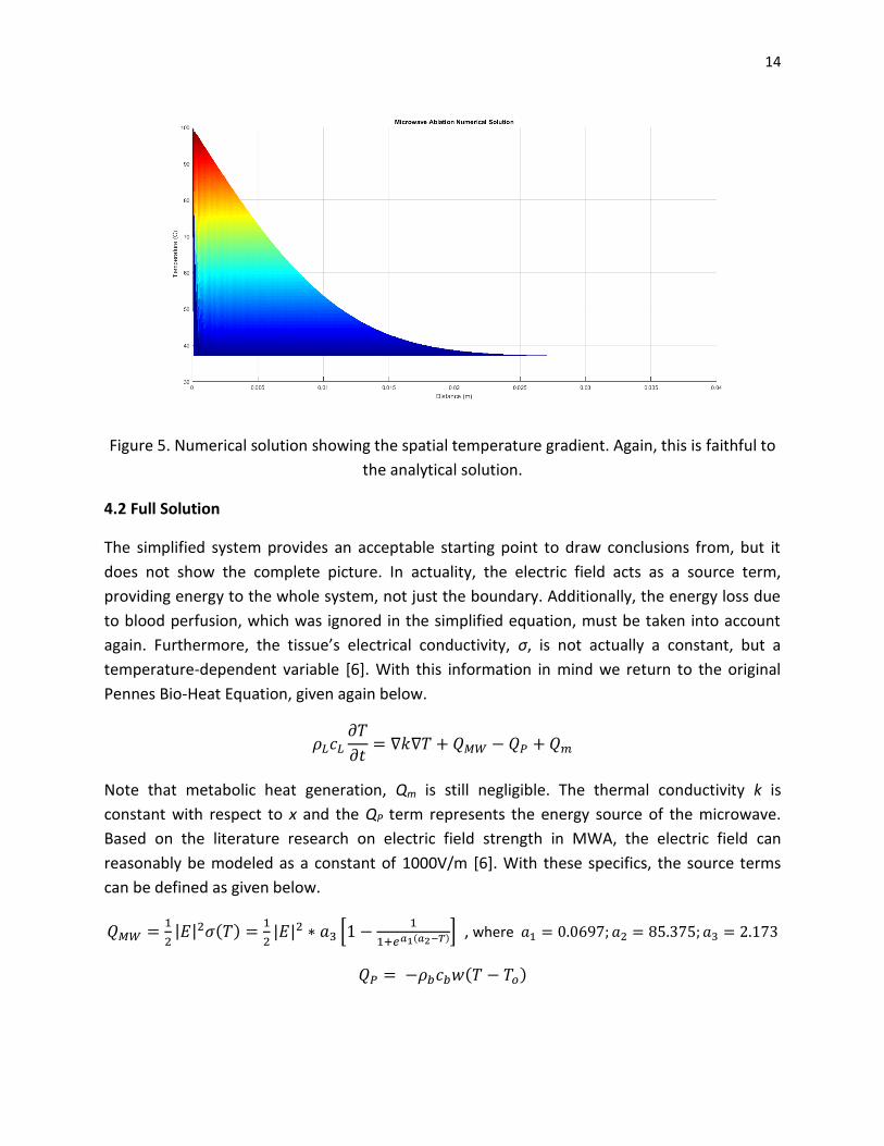
14

Figure 5. Numerical solution showing the spatial temperature gradient. Again, this is faithful to

the analytical solution.

4.2 Full Solution

The simplified system provides an acceptable starting point to draw conclusions from, but it

does not show the complete picture. In actuality, the electric field acts as a source term,

providing energy to the whole system, not just the boundary. Additionally, the energy loss due

to blood perfusion, which was ignored in the simplified equation, must be taken into account

again. Furthermore, the tissue’s electrical conductivity, σ, is not actually a constant, but a

temperature-dependent variable [6]. With this information in mind we return to the original

Pennes Bio-Heat Equation, given again below.

𝜌𝐿𝑐𝐿𝜕𝑇

𝜕𝑡= ∇𝑘∇𝑇 + 𝑄𝑀𝑊 − 𝑄𝑃 +𝑄𝑚

Note that metabolic heat generation, Qm is still negligible. The thermal conductivity k is

constant with respect to x and the QP term represents the energy source of the microwave.

Based on the literature research on electric field strength in MWA, the electric field can

reasonably be modeled as a constant of 1000V/m [6]. With these specifics, the source terms

can be defined as given below.

𝑄𝑀𝑊 =1

2|𝐸|2𝜎(𝑇) =

1

2|𝐸|2 ∗ 𝑎3 [1 −

1

1+𝑒𝑎1(𝑎2−𝑇)] , where 𝑎1 = 0.0697; 𝑎2 = 85.375; 𝑎3 = 2.173

𝑄𝑃 = −𝜌𝑏𝑐𝑏𝑤(𝑇 − 𝑇𝑜)

15

Note that the expression for σ(T) as well as the values for the constants a1- a3 are based on

literature [6]. Substituting these into the Bio-Heat equation gives the full equation,

𝜌𝐿𝑐𝐿𝜕𝑇

𝜕𝑡= 𝑘

𝜕2𝑇

𝜕𝑥2+1

2|𝐸|2𝑎3 [1 −

1

1 + 𝑒𝑎1(𝑎2−𝑇)] − 𝑐𝑏𝑤(𝑇 − 𝑇𝑜)

With initial and boundary conditions,

{

𝑇(𝑥, 0) = 𝑇𝑜𝜕𝑇(0, 𝑡)

𝜕𝑥= 0

𝑇(𝐿, 𝑡) = 𝑇𝑜

Note that the left boundary condition is different here from the simplified model. This zero flux

condition indicates that the temperature is not changing at the location of the microwave

antenna. This is valid because the high temperature and low surface area of microwave

antennae used in ablation result in little heat flux into or out of the probe itself. The other two

conditions are unchanged from the simplified equation.

Solving the full equation in MATLAB using pdepe gives the following results, shown in Figures 6,

7, and 8. The temperature reaches a maximum of 60°C, high enough to cause tissue death [2],

and this level is sustained throughout the full region up until the border, which is cooled to the

level of body temperature by a blood vessel (right boundary condition).

Figure 6. The diffusion of heat across time and space in the full model of hepatic tumor MWA.

16

Figure 7. An alternate view of the full numerical solution, showing the temperature reached vs

the distance from the microwave antenna.

Figure 8. An alternate view of the full numerical solution, showing the temperature reached vs

the duration of treatment.

17

5. Discussion

Due to the nonlinear nature of the tissue electric conductivity and the complexity of the blood

perfusion equation in the governing partial differential equation, a simplified heat conduction

model with modified boundary conditions was derived. As Figures 3 and 5 show, lacking of

driving forces results in a decaying behavior of the temperature profile over the defined

distance, and constant temperatures at the boundaries.

In contrast, the numerical solution to the full equation suggests that under the given initial and

boundary conditions, a constant electric field and blood perfusion give rise to a saturating

behavior as time proceeds as suggested in Figure 7. Moreover, Figure 8 shows that within the

given time window, the temperature reaches the desired lethal point throughout the entire

profile of the tumor tissue and drastically drops to body temperature near the far end

boundary. These observations suggest that the model could serve as the theoretical heat

diffusion model for the first generation MWA since there is no coupling cooling system to help

prevent potential tissue damage due to heat near the far end of the boundary.

A suggested future model that matches the realistic situations should include the development

of the system complexities, i.e. the interactions between microwave and the tissue, as well as

the effect of a cooling agent.

18

References:

[1] Hinshaw, J. L., Lubner, M. G., Ziemlewicz, T. J., Lee Jr, F. T., & Brace, C. L. (2014). Percutaneous tumor ablation tools: microwave, radiofrequency, or cryoablation—what should you use and why?. Radiographics, 34(5), 1344-1362.

[2] Brace, C. L. (2009). Radiofrequency and microwave ablation of the liver, lung, kidney, and bone: what are the differences?. Current problems in diagnostic radiology, 38(3), 135-143.

[3] Prakash, P. (2010). Theoretical Modeling for Hepatic Microwave Ablation. The Open

Biomedical Engineering Journal, 4, 27-38.

[4] Tungjitkusolmun, S., Staelin, S. T., Haemmerich, D., Tsai, J. Z., Cao, H., Webster, J. G., ... &

Vorperian, V. R. (2002). Three-dimensional finite-element analyses for radio-frequency hepatic

tumor ablation. IEEE transactions on biomedical engineering, 49(1), 3-9.

[5] Duck F. (1990). Physical Properties of Tissue: A Comprehensive Reference Book,. Academic

Press, New York. 167–223.

[6] Ji, Z., & Brace, C. L. (2011). Expanded modeling of temperature-dependent dielectric

properties for microwave thermal ablation. Physics in medicine and biology, 56(16), 5249.

19

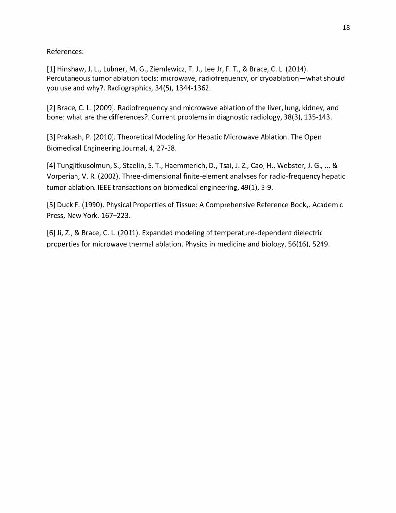
Appendix A: MATLAB Code for Simplified Analytical Solution

%% Microwave Thermal Ablation Analytical Solution clear; clc;

% Constants L = 0.04; % meters k = 0.512;%W/(m*C); thermal conductivity rho_bl = 1000; %blood density; kg/m3 rho_liver = 1060; %liver density; kg/m3 c_bl = 4100; %specific heat of blood J/(kg*C) c_liver = 3600; %specific heat of liver J/(kg*C) w = 0.0064; %Blood perfusion rate; 1/s T_core = 37; %Core temperature; degree C sig = 1.05; %electrical conductivity T_m = 100; %boundary heat condition, provided by the microwave antenna

D = k/(rho_liver*c_liver);

xmesh = 0:.0001:L; tmesh = 0:0.3:300; [xx,tt]=meshgrid(xmesh,tmesh);

T_expansion = zeros(length(tmesh),length(xmesh)) + (T_core-T_m)/L.*xx+T_m; %

Poison Tooth Homogeneous + Particular

for n = 1:5000 a_n = 2*(T_core-T_m)/(n*pi); T = a_n.*sin(n*pi.*xx/L).*exp(-D*(n*pi/L)^2.*tt); T_expansion = T_expansion + T;%T1+T2+T3; end

figure(1) surf(tt,xx,T_expansion,'EdgeColor','none') %surf(tt,-xx,T_expansion,'EdgeColor','none') xlabel('t') ylabel('x') zlabel('T(x,t)') title('Microwave Ablation Analytical Solution') colormap jet

20

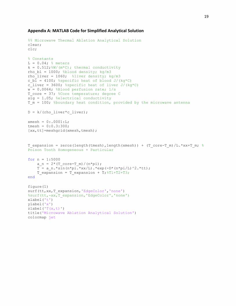
Appendix B: MATLAB Code for Simplified Numerical Solution

%% Microwave Thermal Ablation Analytical Solution clear; clc;

global T_core T_m D L = 0.04; k = 0.512;%W/(m*C); thermal conductivity rho_liver = 1060; %liver density; kg/m3 c_liver = 3600; %specific heat of liver J/(kg*C) T_core = 37; %Core temperature; degree C T_m = 100;

D = k/(rho_liver*c_liver);

xmesh = 0:.0001:L; tmesh = 0:0.3:300; %[xx,tt]=meshgrid(xmesh,tmesh); %% Numerical Solution

sol_pdepe = pdepe(0,@pdefun,@ic,@bc,xmesh,tmesh);

figure(2) hold on surf(tmesh,xmesh,sol_pdepe','Edgecolor','none') %surf(tmesh,-xmesh,sol_pdepe','Edgecolor','none') xlabel('Time (seconds)') ylabel('Distance (m)') zlabel('Temperature (C)') title('Microwave Ablation Numerical Solution') grid on hold off

function [c, f, s] = pdefun(x, t, u, DuDx) global D c = 1; f = D*DuDx; s = 0; end

function u0 = ic(x) global T_core u0 = T_core; end

function [pl,ql,pr,qr] = bc(xl,ul,xr,ur,t) global T_m T_core pl = ul-T_m; ql = 0; pr = ur-T_core; qr = 0; end

21

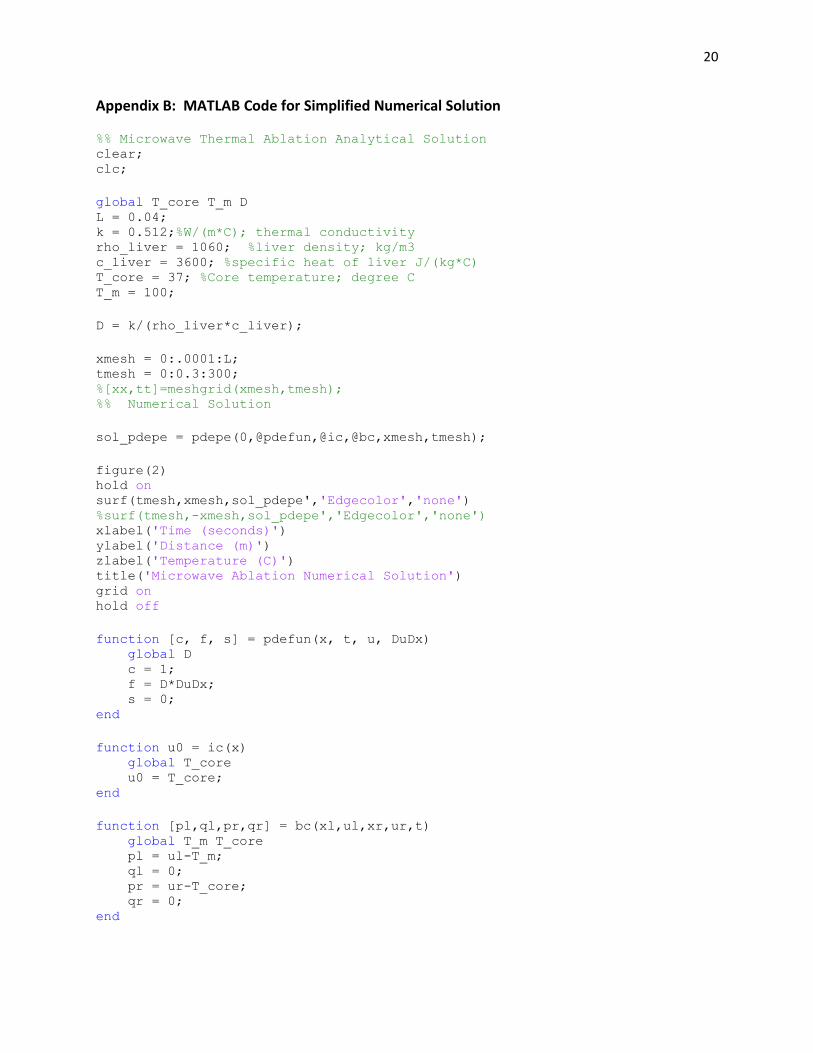
Appendix C: MATLAB Code for Final Numerical Solution

%BENG 221 Project Microwave ablation of a hepatic tumor (numerical solution

to the original bioheat function)

close all; clc

%Constants

global D U E a1 a2 a3 T_0 rho_liver c_liver

k = 0.512;%W/(m*K); thermal conductivity

rho_bl = 1000; %blood density; kg/m3

rho_liver = 1060; %liver density; kg/m3

c_bl = 4180; %specific heat of blood J/(kg*K)

c_liver = 3600; %specific heat of liver J/(kg*K)

w = 0.0064; %Blood perfusion rate; 1/s

T_0 =37; %Initial temperature

a1 =0.0697; %a1-3 constants for electric conductivity constant

a2=85.375;

a3=2.173;

E = 800; % average electric field

xmesh =0:0.0001:0.06; %distance range in m

tmesh = 0:0.1:300; %time duration in s

D = k/(rho_liver*c_liver); % Rearranged diffusion constant

U = rho_bl*c_bl*w/(rho_liver*c_liver);

%% Plotting using pdepe

sol_pdepe = pdepe(0,@pdefun,@ic,@bc,xmesh,tmesh);

figure ()

surf(tmesh,xmesh,sol_pdepe', 'EdgeColor','none')

title('Numerical Solution to the Original Pennes Bioheat Equation using pdepe

function ')

xlabel('Time (s)')

ylabel('Distance (m)')

zlabel('Temperature (°C)')

%% Partial differential equation function

function [c, f, s] = pdefun(x, t, T, DTDx)

% PDE coefficients functions

global D U a1 a2 a3 T_0 E rho_liver c_liver

c = 1;

f = D * DTDx;

%Driving forces, heat generation and blood perfusion

s = -U*(T-T_0)+ E^2/(2*rho_liver*c_liver)...

*(a3*(1-1/(1+exp(a1*(a2-T)))));

end

% --------------------------------------------------------------

%Initial condition function

function T0 = ic(x)

T0 = 37; %degree C

end

% --------------------------------------------------------------

%Boundary conditions function

function [pl, ql, pr, qr] = bc(xl, Tl, xr, Tr, t)

pl = 0; % No flux left boundary condition

ql = 1; % No flux left boundary condition

pr = Tr-37; % Constant rigt boundary condition

qr = 0; % Constant rigt boundary condition

end