Page 1
Thermal-fluid simulation of nuclear steam generator performance
using Flownex and RELAP5/mod3.4
Charl Cilliers
Supervisor: Prof. P.G. Rousseau
Thesis submitted to the University of the North-West, Potchefstroom, in partial
fulfilment for the degree of
Master of Engineering (Nuclear Science and Engineering)
December 2012
Page 2
Dedicated to the eternal pursuit of knowledge.
i
Page 3
Abstract
The steam generator plays a primary role in the safety and performance of a pressurized water
reactor nuclear power plant. The cost to utilities is in the order of millions of Rands a year as a
direct result of damage to steam generators. The damage results in lower efficiency or even plant
shutdown. It is necessary for the utility and for academia to have models of nuclear components
by which research and analysis may be performed. It must be possible to analyse steam generator
performance for both day-to-day operational analysis as well as in the case of extreme accident
scenarios.
The homogeneous model for two-phase flow is simpler in its implementation than the two-fluid
model, and therefore suffers in accuracy. Its advantage lies in its quick turnover time for
development of models and subsequent analysis. It is often beneficial for a modeller to be able to
quickly set up and analyse a model of a system, and a trade-off between accuracy and
time-management is thus required.
Searches through available literature failed to provide answers to how the homogeneous model
compares with the two-fluid model for operational and safety analysis. It is expected to see
variations between the models, from the analysis of the mathematics, but it remains to be shown
what these differences are.
The purpose of this study was to determine how the homogeneous model for two-phase flow
compares with the two-fluid model when applied to a u-tube steam generator of a typical
pressurized water reactor. The steam generator was modelled in both RELAP5 and in Flownex.
A custom script was written for Flownex in order to implement the Chen correlation for boiling
heat transfer. This was significantly less detailed than RELAP5’s solution of a matrix of flow
regimes and heat transfer correlations. The geometry of the models were based on technical
drawings from Koeberg Nuclear Power Plant, and were simplified to a one-dimensional model.
Plant data obtained from Koeberg was used to validate the models at 100%, 80% and 60% power
output.
It was found that the overall heat transfer rate predicted with the RELAP5 two-fluid model was
within 1.5% of the measured data from the Koeberg plant. The results generated by the
homogeneous model for the overall heat transfer were within 4.5% of the measured values.
ii
Page 4
However, the differences in the detailed temperature distributions and heat transfer coefficient
values were quite significant at the inlet and outlet ends of the tube bundle, at the bottom tube
sheet of the steam generator. In this area the water-level was not accurately modelled by the
homogeneous model, and therefore there was an under-prediction in heat transfer in that region.
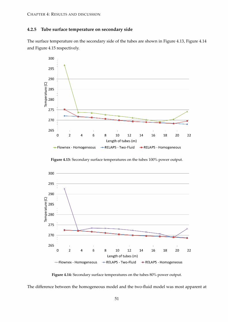
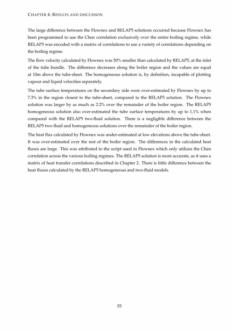
Large differences arose between the Flownex and RELAP5 solutions due to difference in the heat
transfer correlations used. The Flownex model exclusively implemented the Chen correlation,
while RELAP5 implements a flow regime map correlated to a table of heat transfer correlations.
It was concluded that the results from the homogeneous model for two-phase flow do not differ
significantly when compared with the two-fluid model when applied to the u-tube steam
generator at the normal operating conditions. Significant differences do, however, occur in lower
regions of the boiler where the quality is lower. We conclude that the homogeneous model offers
significant advantage in simplicity over the two-fluid model for normal operational analysis.
This may not be the case for detailed accident analysis, which was beyond the scope of this study.
Keywords: Nuclear engineering, pressurized water reactor, U-tube steam generator, Flownex,
RELAP5, thermal-fluid simulation
iii
Page 5
Acknowledgements
I would like to thank Professor Pieter Rousseau for his critical input as advisor and study leader
for this project. Thanks go to the Department of Science and Technology and the National
Research Foundation for financial assistance of this study. I would also like to thank Tommy
Booysen and Randolph Damon from Koeberg Nuclear Power Plant (ESKOM) for dedicating time
and putting in effort to provide data and support for the study. Furthermore, engineers at
M-Tech Industrial who provided valuable input on the Flownex simulation, for which I am
thankful for, were William Theron and Faan Oelofse. Lastly, thanks need to go to my family and
friends. My parents, my uncle, my brother and the close support structure of friends that have all
unknowingly contributed to this work in many ways.
Disclaimer
This work is based upon research supported by the South African Research Chairs Initiative of the
Department of Science and Technology and National Research Foundation.
Any opinion, findings and conclusions or recommendations expressed in this material are those
of the author(s) and therefore the NRF and DST do not accept any liability with regard thereto.
iv
Page 6
Contents
1 Introduction 1
1.1 Background . . . . . . . . . . . . . . . . . . . . . . . . . . . . . . . . . . . . . . . . . . 1
1.1.1 Pressurised Water Reactors . . . . . . . . . . . . . . . . . . . . . . . . . . . . . 2
1.1.2 Steam Generators . . . . . . . . . . . . . . . . . . . . . . . . . . . . . . . . . . . 2
1.1.3 Computer Modelling and Simulation of Steam Generators . . . . . . . . . . . 4
1.2 Motivation . . . . . . . . . . . . . . . . . . . . . . . . . . . . . . . . . . . . . . . . . . . 5
1.3 Problem Statement . . . . . . . . . . . . . . . . . . . . . . . . . . . . . . . . . . . . . . 6
1.4 Methodology . . . . . . . . . . . . . . . . . . . . . . . . . . . . . . . . . . . . . . . . . 6
2 Overview of the Literature 8
2.1 Issues facing Steam Generator operators . . . . . . . . . . . . . . . . . . . . . . . . . . 8
2.1.1 Degradation of the primary side . . . . . . . . . . . . . . . . . . . . . . . . . . 8
2.1.2 Degradation of the secondary side . . . . . . . . . . . . . . . . . . . . . . . . . 9
2.1.3 The cost effect of degradation . . . . . . . . . . . . . . . . . . . . . . . . . . . . 9
2.1.4 The effect of degradation on heat transfer and efficiency . . . . . . . . . . . . 9
2.1.5 Concluding remarks regarding issues faced in steam generator operation . . 10
2.2 Thermal-fluid models of two-phase flow . . . . . . . . . . . . . . . . . . . . . . . . . . 11
2.2.1 Multi-phase flow and phase transitions . . . . . . . . . . . . . . . . . . . . . . 11
2.2.2 Chen correlation for the nucleate boiling heat transfer coefficient . . . . . . . 14
2.2.3 Two-fluid model . . . . . . . . . . . . . . . . . . . . . . . . . . . . . . . . . . . 16
2.2.4 Homogeneous model . . . . . . . . . . . . . . . . . . . . . . . . . . . . . . . . 17
2.3 Simulating steam generators using thermal-hydraulic codes . . . . . . . . . . . . . . 18
2.3.1 Flownex . . . . . . . . . . . . . . . . . . . . . . . . . . . . . . . . . . . . . . . . 19
v
Page 7
CONTENTS
2.3.2 RELAP5/Mod3.4 . . . . . . . . . . . . . . . . . . . . . . . . . . . . . . . . . . . 20
2.3.3 Previous work on steam generator models . . . . . . . . . . . . . . . . . . . . 21
3 Basis for the Models 22
3.1 Data obtained from Koeberg Nuclear Power Station . . . . . . . . . . . . . . . . . . . 22
3.1.1 Statistical analysis of the data . . . . . . . . . . . . . . . . . . . . . . . . . . . . 24
3.2 Preliminary steady-state calculations . . . . . . . . . . . . . . . . . . . . . . . . . . . . 27
3.3 Simplification of the geometry . . . . . . . . . . . . . . . . . . . . . . . . . . . . . . . . 29
3.4 Geometry and Heat Structure inputs . . . . . . . . . . . . . . . . . . . . . . . . . . . . 34
3.5 Model Development . . . . . . . . . . . . . . . . . . . . . . . . . . . . . . . . . . . . . 35
3.5.1 RELAP5 - Two-Fluid . . . . . . . . . . . . . . . . . . . . . . . . . . . . . . . . . 35
3.5.2 RELAP5 - Homogeneous . . . . . . . . . . . . . . . . . . . . . . . . . . . . . . 37
3.5.3 Flownex . . . . . . . . . . . . . . . . . . . . . . . . . . . . . . . . . . . . . . . . 38
4 Results and discussion 41
4.1 Comparison with empirical data . . . . . . . . . . . . . . . . . . . . . . . . . . . . . . 41
4.1.1 100% Power Output . . . . . . . . . . . . . . . . . . . . . . . . . . . . . . . . . 41
4.1.2 80% Power Output . . . . . . . . . . . . . . . . . . . . . . . . . . . . . . . . . . 42
4.1.3 60% Power Output . . . . . . . . . . . . . . . . . . . . . . . . . . . . . . . . . . 42
4.2 Detailed inter-model comparisons . . . . . . . . . . . . . . . . . . . . . . . . . . . . . 43
4.2.1 Primary side temperatures . . . . . . . . . . . . . . . . . . . . . . . . . . . . . 43
4.2.2 Quality through the boiler . . . . . . . . . . . . . . . . . . . . . . . . . . . . . . 45
4.2.3 Heat transfer coefficient on the surface of the tubes . . . . . . . . . . . . . . . 47
4.2.4 Flow velocity through the boiler region . . . . . . . . . . . . . . . . . . . . . . 48
4.2.5 Tube surface temperature on secondary side . . . . . . . . . . . . . . . . . . . 51
4.2.6 Heat flux on the surface of the tubes . . . . . . . . . . . . . . . . . . . . . . . . 52
4.3 Summary of inter-model comparison . . . . . . . . . . . . . . . . . . . . . . . . . . . . 54
5 Conclusions and Recommendations 56
5.1 Conclusions . . . . . . . . . . . . . . . . . . . . . . . . . . . . . . . . . . . . . . . . . . 56
5.2 Improvements and Recommendations . . . . . . . . . . . . . . . . . . . . . . . . . . . 59
vi
Page 8
CONTENTS
6 Potential for Future Work 61
6.1 Model improvements . . . . . . . . . . . . . . . . . . . . . . . . . . . . . . . . . . . . . 61
6.2 Model alterations . . . . . . . . . . . . . . . . . . . . . . . . . . . . . . . . . . . . . . . 61
6.3 Transient analysis . . . . . . . . . . . . . . . . . . . . . . . . . . . . . . . . . . . . . . . 61
6.4 Model extensions . . . . . . . . . . . . . . . . . . . . . . . . . . . . . . . . . . . . . . . 62
References 63
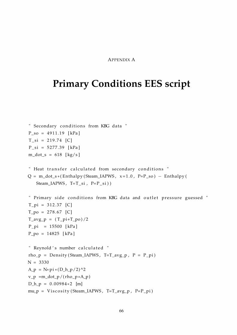
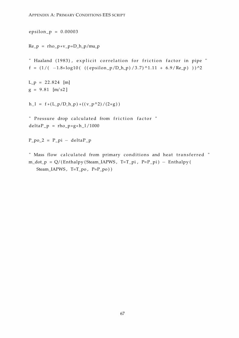
A Primary Conditions EES script 66
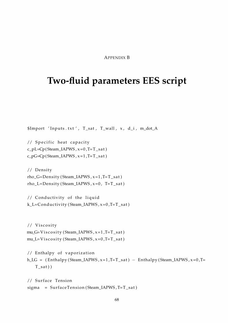
B Two-fluid parameters EES script 68
C Chen correlation C# script 70
D RELAP5 Code 80
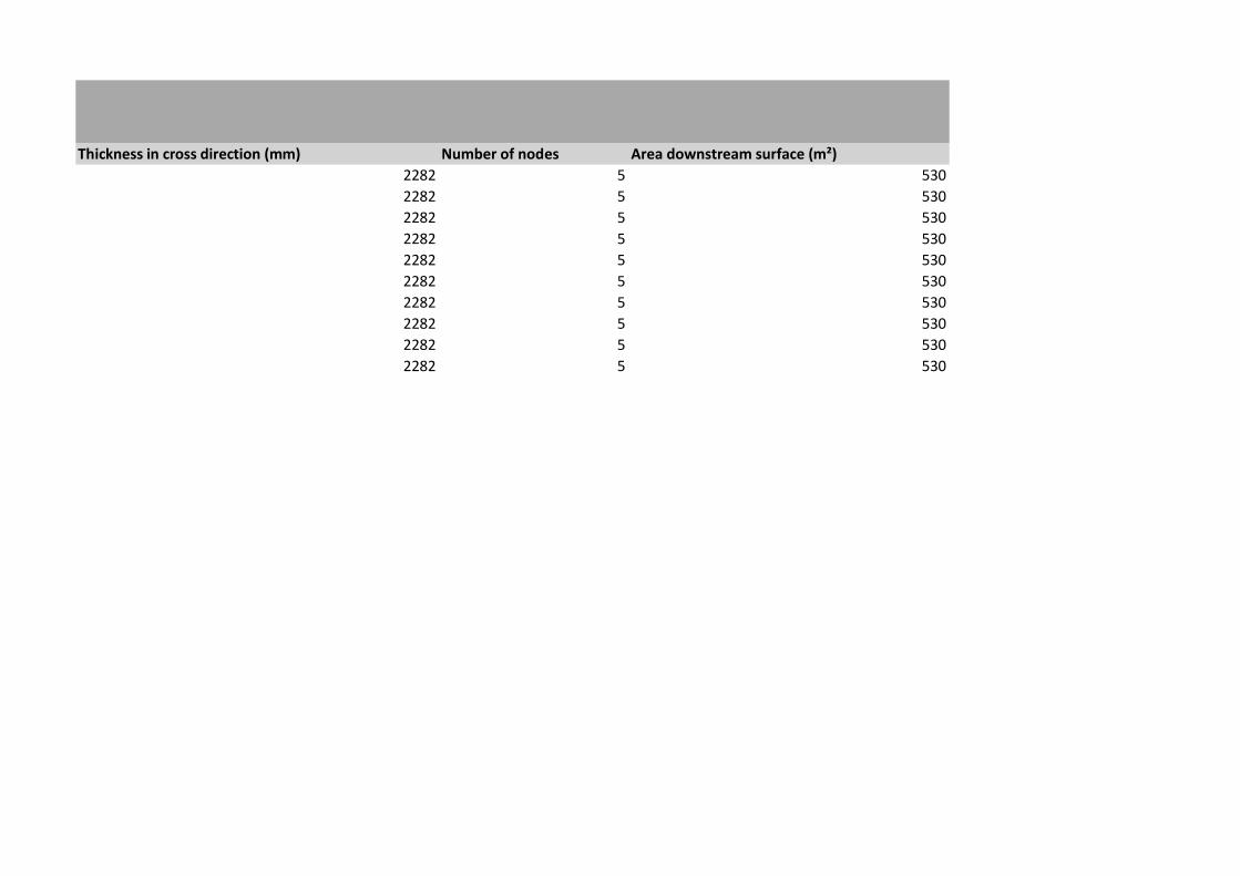
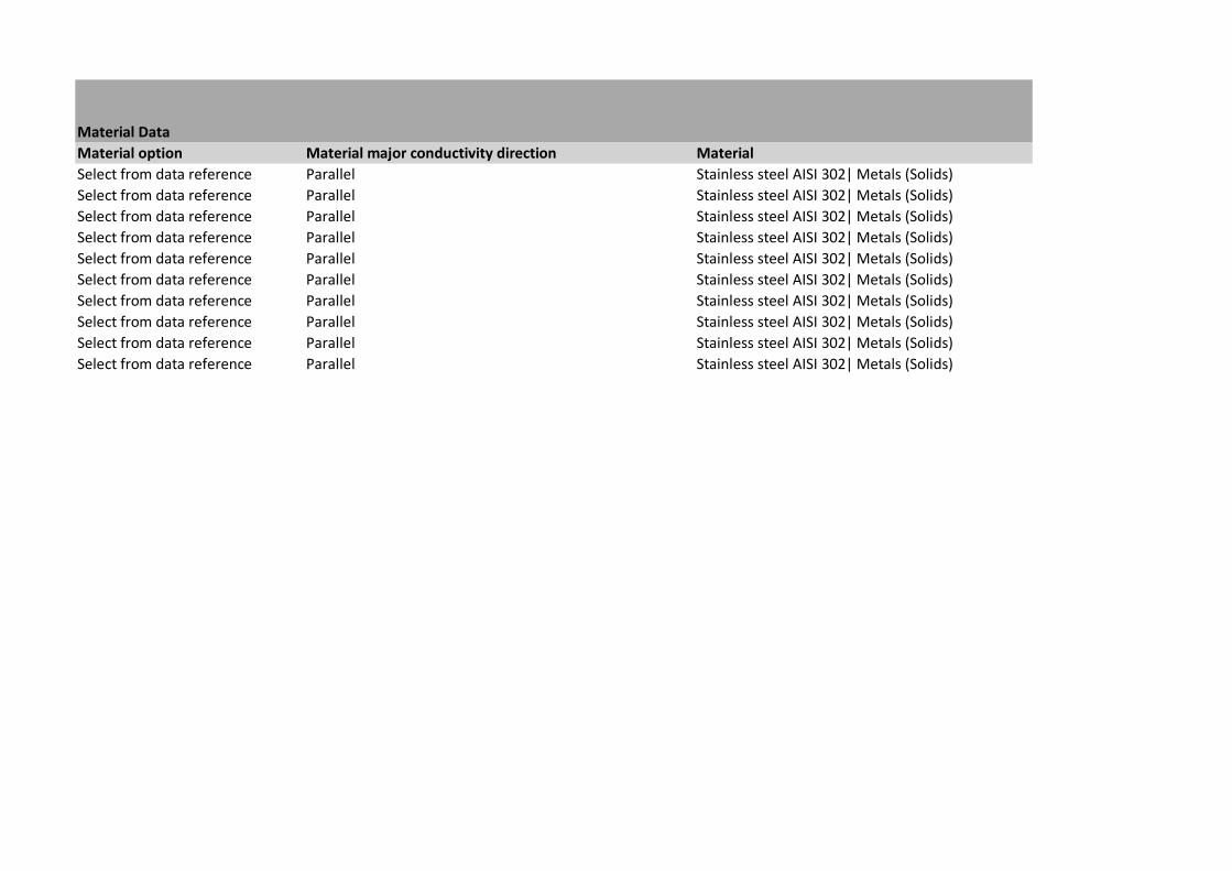
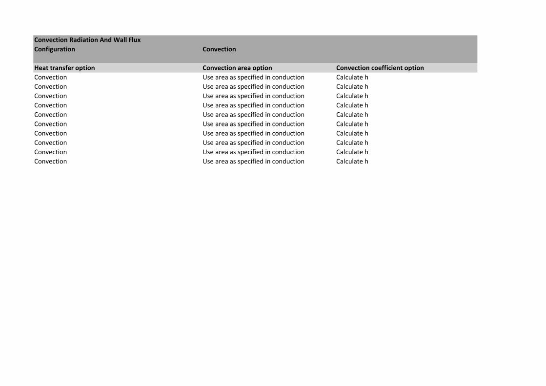
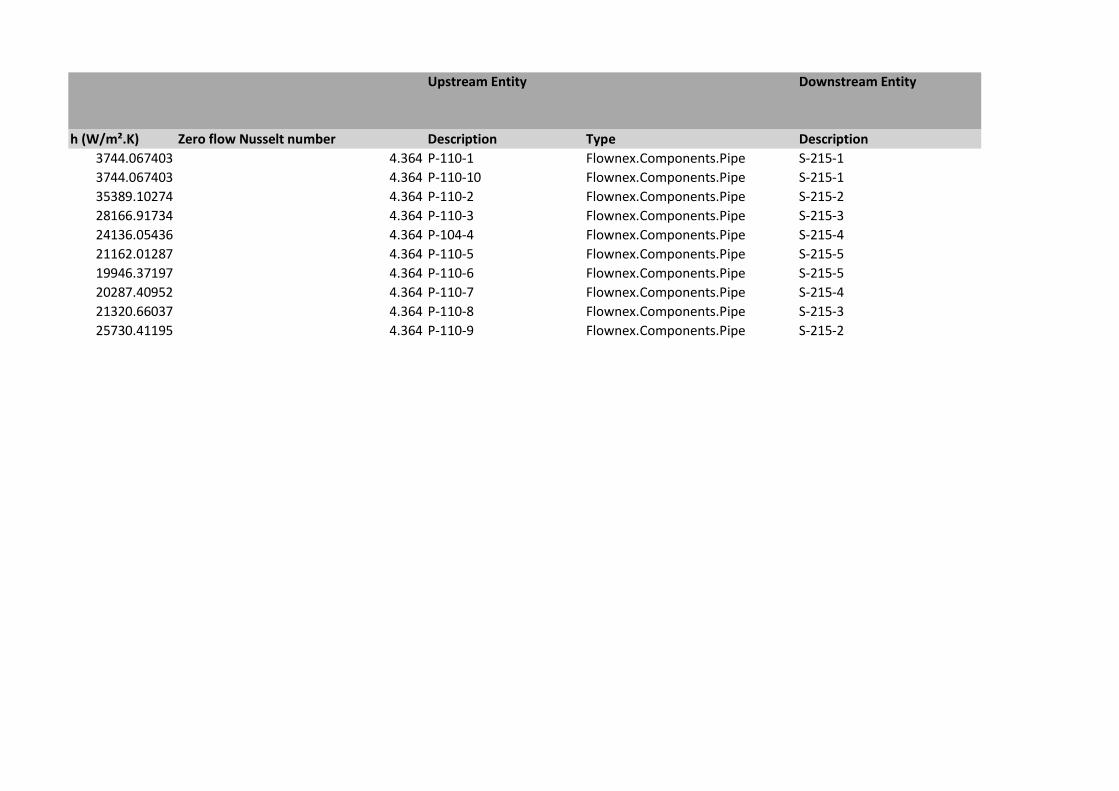
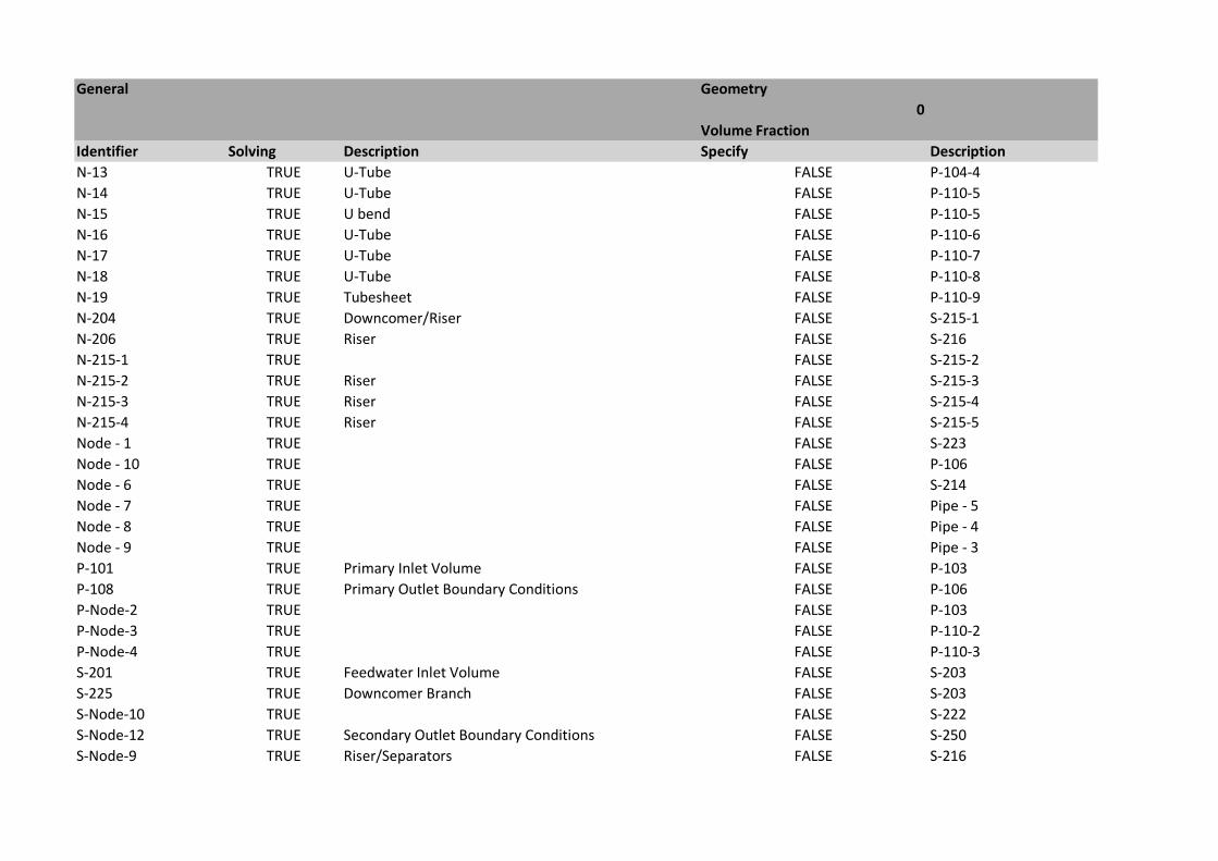
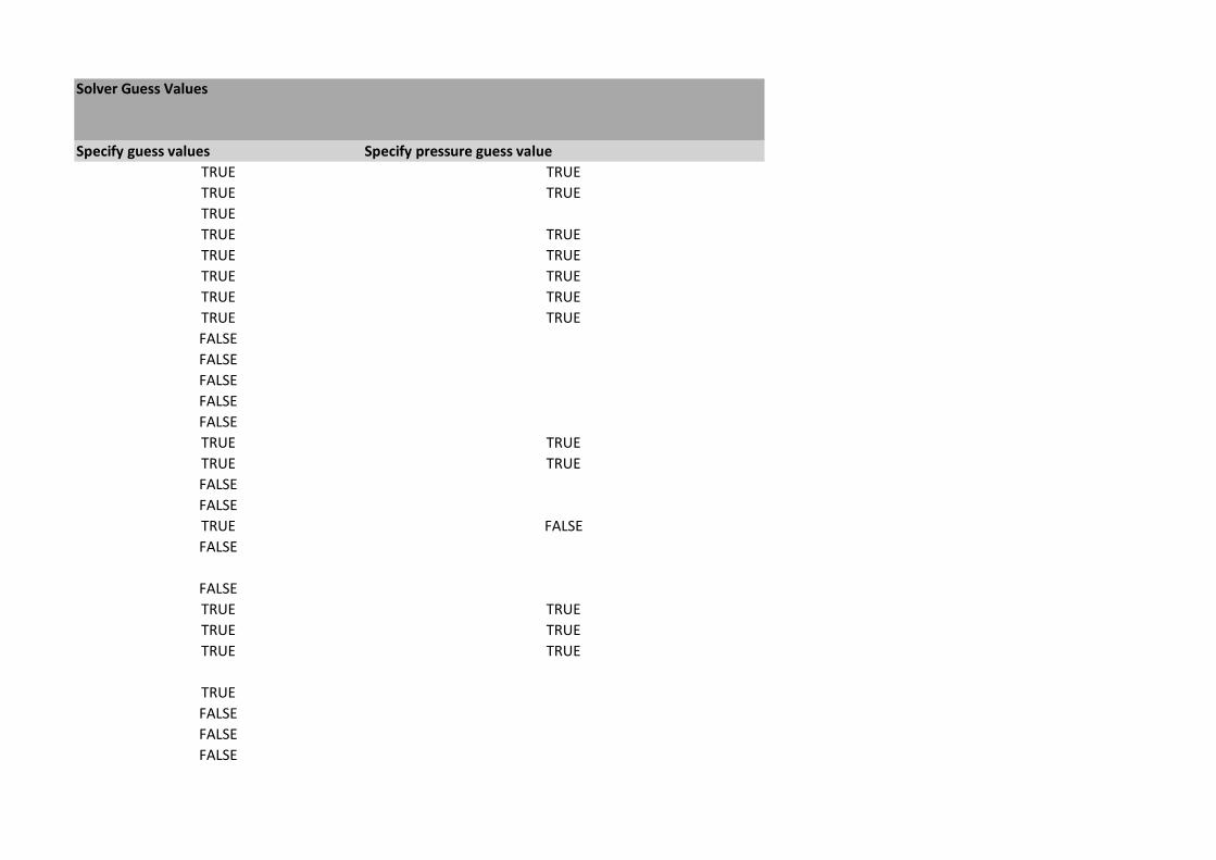
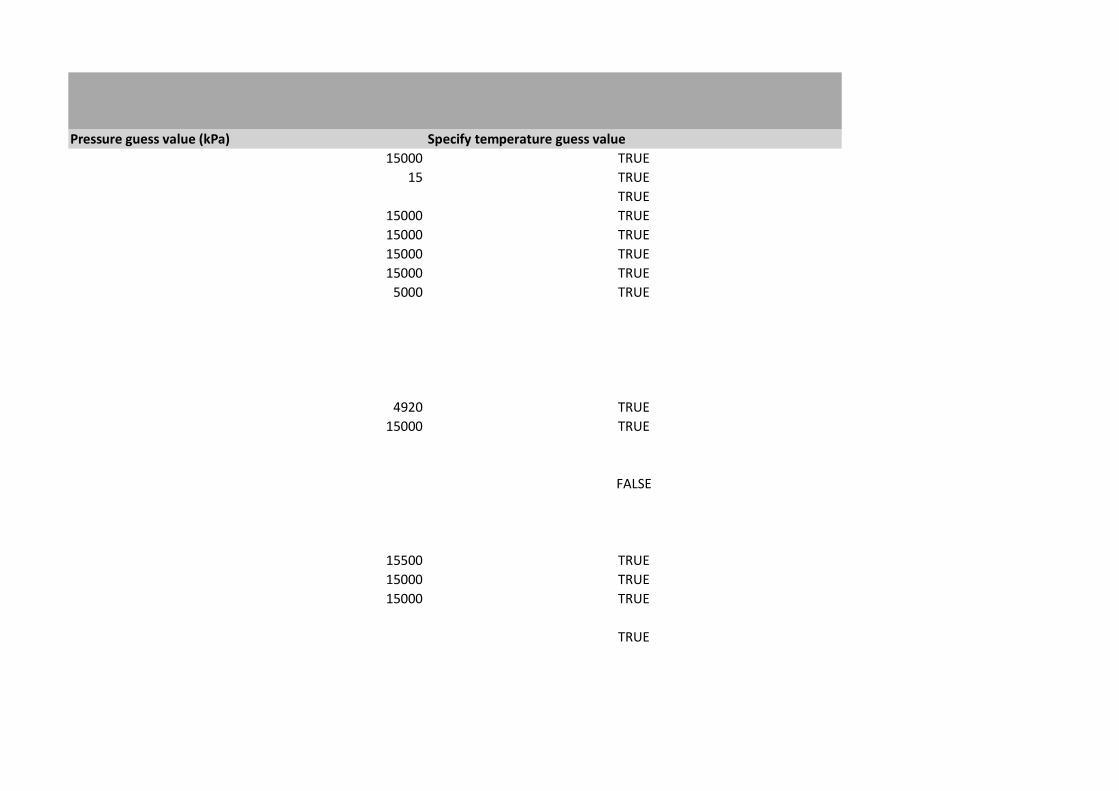
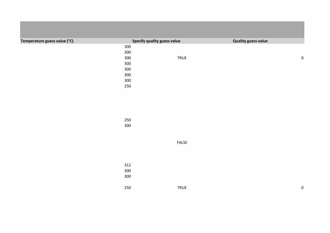
E Inputs to the Flownex Model 96
vii
Page 9
List of Figures
1.1 Simplified diagram of a PWR connected to the power-producing side of the power
plant (Kok, 2009) . . . . . . . . . . . . . . . . . . . . . . . . . . . . . . . . . . . . . . . 3
1.2 Diagram of a typical steam generator used in a PWR (Bonavigo and de Salve, 2011) . 3
1.3 Quantitative research methodology with model development . . . . . . . . . . . . . 7
2.1 Various boiling regimes that occur within a two-phase fluid (Ishii and Hibiki, 2006) . 12
2.2 Flow regime matrix for vertical flow used in RELAP5 for boiling heat transfer
calculations (RELAP5, 2001c) . . . . . . . . . . . . . . . . . . . . . . . . . . . . . . . . 13
2.3 The boiling and condensing curve used by RELAP5 to calculate heat flux (RELAP5,
2001b) . . . . . . . . . . . . . . . . . . . . . . . . . . . . . . . . . . . . . . . . . . . . . 14
2.4 Typical nodalization for the model of a steam generator . . . . . . . . . . . . . . . . 18
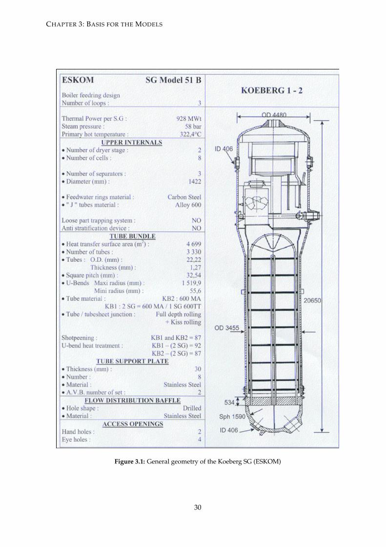
3.1 General geometry of the Koeberg SG (ESKOM) . . . . . . . . . . . . . . . . . . . . . . 30
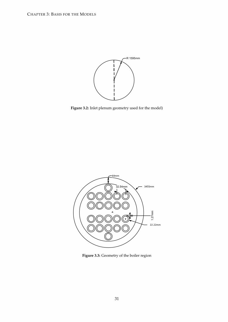
3.2 Inlet plenum geometry used for the model) . . . . . . . . . . . . . . . . . . . . . . . . 31
3.3 Geometry of the boiler region . . . . . . . . . . . . . . . . . . . . . . . . . . . . . . . . 31
3.4 Geometry of the riser region . . . . . . . . . . . . . . . . . . . . . . . . . . . . . . . . . 32
3.5 Geometry of the separator region . . . . . . . . . . . . . . . . . . . . . . . . . . . . . . 32
3.6 Geometry of the dryer region . . . . . . . . . . . . . . . . . . . . . . . . . . . . . . . . 33
3.7 Geometry of the steam dome region . . . . . . . . . . . . . . . . . . . . . . . . . . . . 33
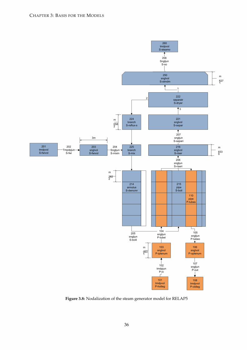
3.8 Nodalization of the steam generator model for RELAP5 . . . . . . . . . . . . . . . . . 36
3.9 Nodalization of the steam generator model for Flownex . . . . . . . . . . . . . . . . . 38
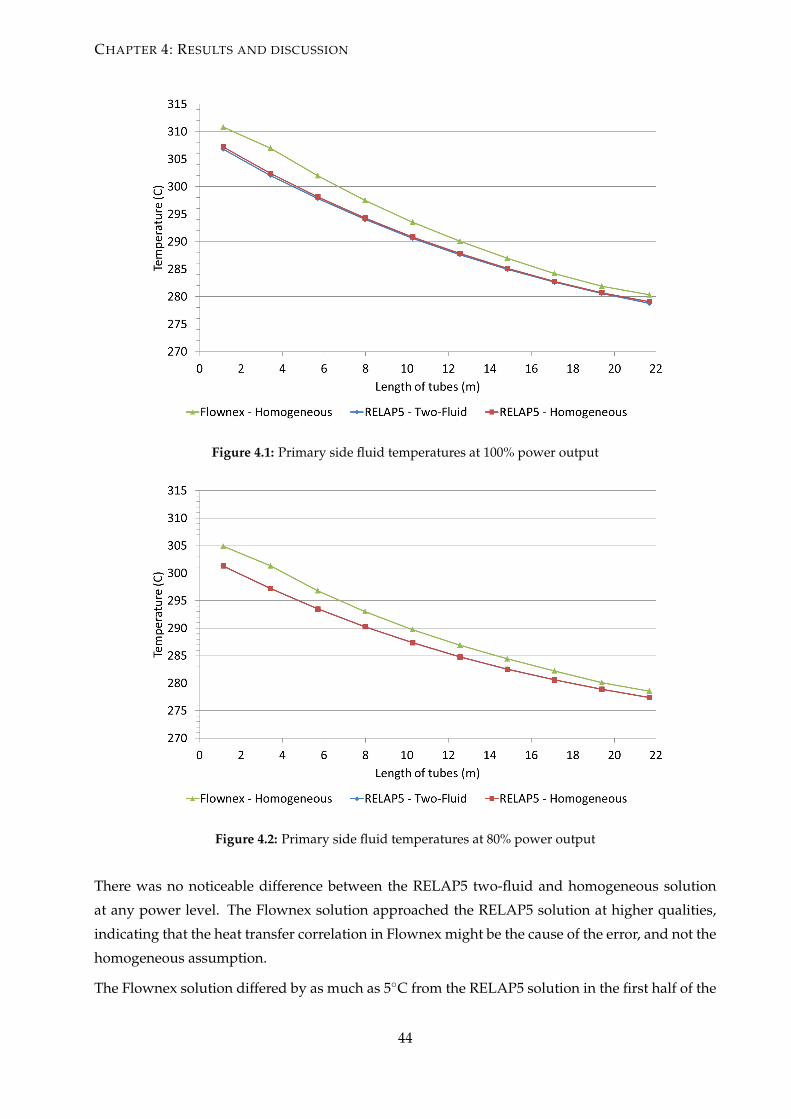
4.1 Primary side fluid temperatures at 100% power output . . . . . . . . . . . . . . . . . 44
4.2 Primary side fluid temperatures at 80% power output . . . . . . . . . . . . . . . . . . 44
4.3 Primary side fluid temperatures at 60% power output . . . . . . . . . . . . . . . . . . 45
viii
Page 10
LIST OF FIGURES
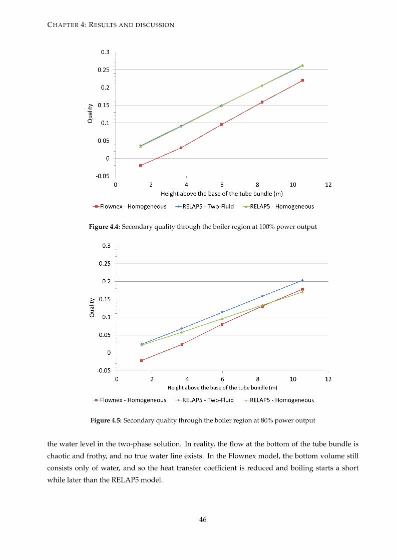
4.4 Secondary quality through the boiler region at 100% power output . . . . . . . . . . 46
4.5 Secondary quality through the boiler region at 80% power output . . . . . . . . . . . 46
4.6 Secondary quality through the boiler region at 60% power output . . . . . . . . . . . 47
4.7 Heat transfer coefficient on the surface of the tubes at 100% power output. . . . . . . 48
4.8 Heat transfer coefficient on the surface of the tubes at 80% power output. . . . . . . 48
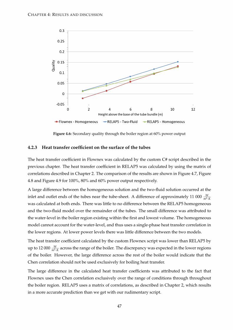
4.9 Heat transfer coefficient on the surface of the tubes at 60% power output. . . . . . . 49
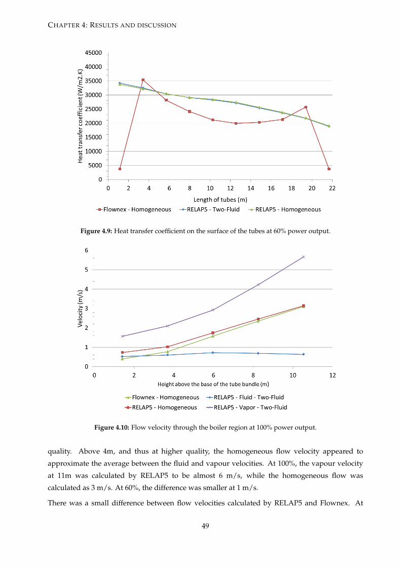
4.10 Flow velocity through the boiler region at 100% power output. . . . . . . . . . . . . . 49
4.11 Flow velocity through the boiler region at 80% power output. . . . . . . . . . . . . . 50
4.12 Flow velocity through the boiler region at 60% power output. . . . . . . . . . . . . . 50
4.13 Secondary surface temperatures on the tubes 100% power output. . . . . . . . . . . . 51
4.14 Secondary surface temperatures on the tubes 80% power output. . . . . . . . . . . . 51
4.15 Secondary surface temperatures on the tubes 60% power output. . . . . . . . . . . . 52
4.16 Heat flux on the surface of the tubes at 100% power output. . . . . . . . . . . . . . . 53
4.17 Heat flux on the surface of the tubes at 80% power output. . . . . . . . . . . . . . . . 53
4.18 Heat flux on the surface of the tubes at 60% power output. . . . . . . . . . . . . . . . 54
ix
Page 11
List of Tables
2.1 Heat transfer correlations used in the various boiling regimes for RELAP5 . . . . . . 13
2.2 Heat transfer correlations used in the various boiling regimes for Flownex . . . . . . 14
2.3 Advantages and Disadvantages to using Flownex and the homogeneous model. . . 20
2.4 Advantages and Disadvantages to using RELAP5 and the two-fluid model. . . . . . 20
3.1 Sample of the steady-state data obtained from a single unit at Koeberg Nuclear
Power Station . . . . . . . . . . . . . . . . . . . . . . . . . . . . . . . . . . . . . . . . . 23
3.2 Statistical analysis of steady-state plant operating data at 100% power output. . . . . 25
3.3 Statistical analysis of steady-state plant operating data at 80% power output. . . . . 26
3.4 Statistical analysis of steady-state plant operating data at 60% power output. . . . . 27
3.5 Volumetric inputs for the steam generator model . . . . . . . . . . . . . . . . . . . . . 34
3.6 Heat structure inputs for the steam generator model . . . . . . . . . . . . . . . . . . . 35
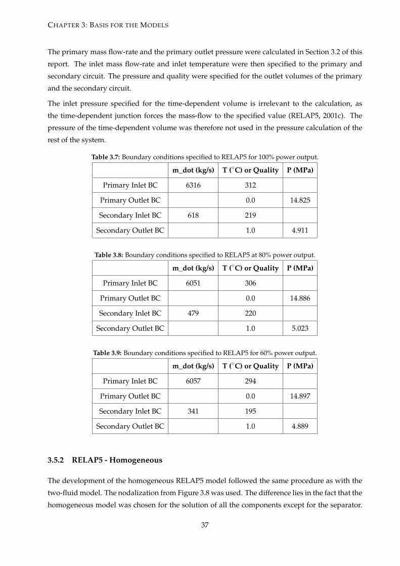
3.7 Boundary conditions specified to RELAP5 for 100% power output. . . . . . . . . . . 37
3.8 Boundary conditions specified to RELAP5 at 80% power output. . . . . . . . . . . . . 37
3.9 Boundary conditions specified to RELAP5 for 60% power output. . . . . . . . . . . . 37
3.10 Boundary conditions specified to Flownex for 100% power output. . . . . . . . . . . 39
3.11 Boundary conditions specified to Flownex for 80% power output. . . . . . . . . . . . 40
3.12 Boundary conditions specified to Flownex at 60% power output. . . . . . . . . . . . . 40
4.1 Steady-state validation of the model at 100% power output . . . . . . . . . . . . . . . 41
4.2 Steady-state validation of the model at 80% power output . . . . . . . . . . . . . . . 42
4.3 Steady-state validation of the model at 60% power output . . . . . . . . . . . . . . . 43
x
Page 12
Nomenclature
Terms and Acronyms
CFD Computational Fluid Dynamics
CFD Computational Fluid Dynamics
EPRI Electric Power Research Institute
HTGR High Temperature Gas Reactor
LOCA Loss of Coolant Accident
MSLB Main Steam Line Break
NNR South African National Nuclear Regulator
nodalization A network of nodes and components connected to form a system, shown in diagram
form in Figure 2.4
NPP Nuclear Power Plant
PWR Pressurised Water Reactor
SG Steam Generator
SSE Safe Shut-down in event of Earthquake
UTSG U-tube Steam Generator
Constants and Variables
m Mass flow-rate (kg/s)
A Area (m2)
αk The void fraction of phase k
αkw Void fraction at the wall
xi
Page 13
NOMENCLATURE
Γk Mass generation for phase k
µ Viscosity ( kgm·s )
ρ Density ( kgm3 )
ρk Density of phase k (kg/m2)
Σ Stress tensor (Navier-stokes)
ΣT Turbulent stress tensor
τkw Shear stress at the wall
Mdk Inter-facial shear force
ζh Heated perimeter (m)
Chk Distribution parameter for the k phase enthalpy
Dh Hydraulic diameter (m)
di Inner diameter of the tubes
do Outer diameter (m)
hi Inlet enthalpy (kJ/kg)
ho Outlet enthalpy (kJ/kg)
kL Coefficient of heat conduction for the liquid
kw Thermal conductivity of the wall material ( Wm2K )
pst Saturation pressure (Pa)
q′′kw Heat flux at the wall (W/m2)
R f Fouling factor, or resistance to heat transfer due to fouling ( m2KW )
Re Reynolds number - dimensionless
v Flow velocity ( ms )
vk Average velocity of phase k (m/s)
ht p, hnb, hcb Heat transfer coefficients for two-phase flow, nucleate boiling and convective boiling
respectively
U Over-all heat transfer coefficient ( Wm2·K )
xii
Page 14
CHAPTER 1
Introduction
1.1 Background
Nuclear power plants around the world produced 369 Gigawatts of electricity at the end of 2011
(IAEA, 2012). The types of nuclear reactors are described in various introductory texts (Lamarsh
and Baratta, 2001; Lewis, 2008; Shultis and Faw, 2002). Most nuclear reactors sustain a fission
chain reaction which provides heat to a flowing coolant. The coolant may either boil and drive a
set of turbines directly, or it may be under pressure and transfer heat to a secondary side used for
boiling and power generation. As of March 2012, there were 436 nuclear power plants (NPP) in
operation around the world, of which 272 were pressurised water reactors (PWR) (IAEA, 2012).
PWRs thus accounted for 67% of the installed nuclear power capacity. In addition, 51 of the
63 new reactors under construction around the world as of early 2012 are also of the PWR type
(IAEA, 2012). The PWR’s critical primary components include the nuclear reactor, pressurizer and
steam generators (SG). The SGs transfer the primary side heat to feed-water on the secondary side,
producing steam. The steam is then used to drive a set of turbines that produces electrical power.
The SGs in PWRs are designed for temperatures up to 340◦C and pressures up to 18 MPa. In
addition to the extreme conditions, the components are susceptible to many forms of degradation
such as corrosion and mechanical wear from fluid induced vibrations. The two-phase boiling
phenomenon occurs during the production of steam and is a complex process to model accurately.
The information gained from an accurate thermal-fluid analysis may include predictions of local
flow velocity, temperature, pressure and quality. These parameters are beneficial to the study of
chemical reaction theory, solid deposition and water-hammer, all of which may impact negatively
on SG performance.
A valid model of a steam generator is beneficial for predicting local flow parameters that may be
used to supplement more complex studies of SG degradation or to make operational decisions.
1
Page 15
CHAPTER 1: INTRODUCTION
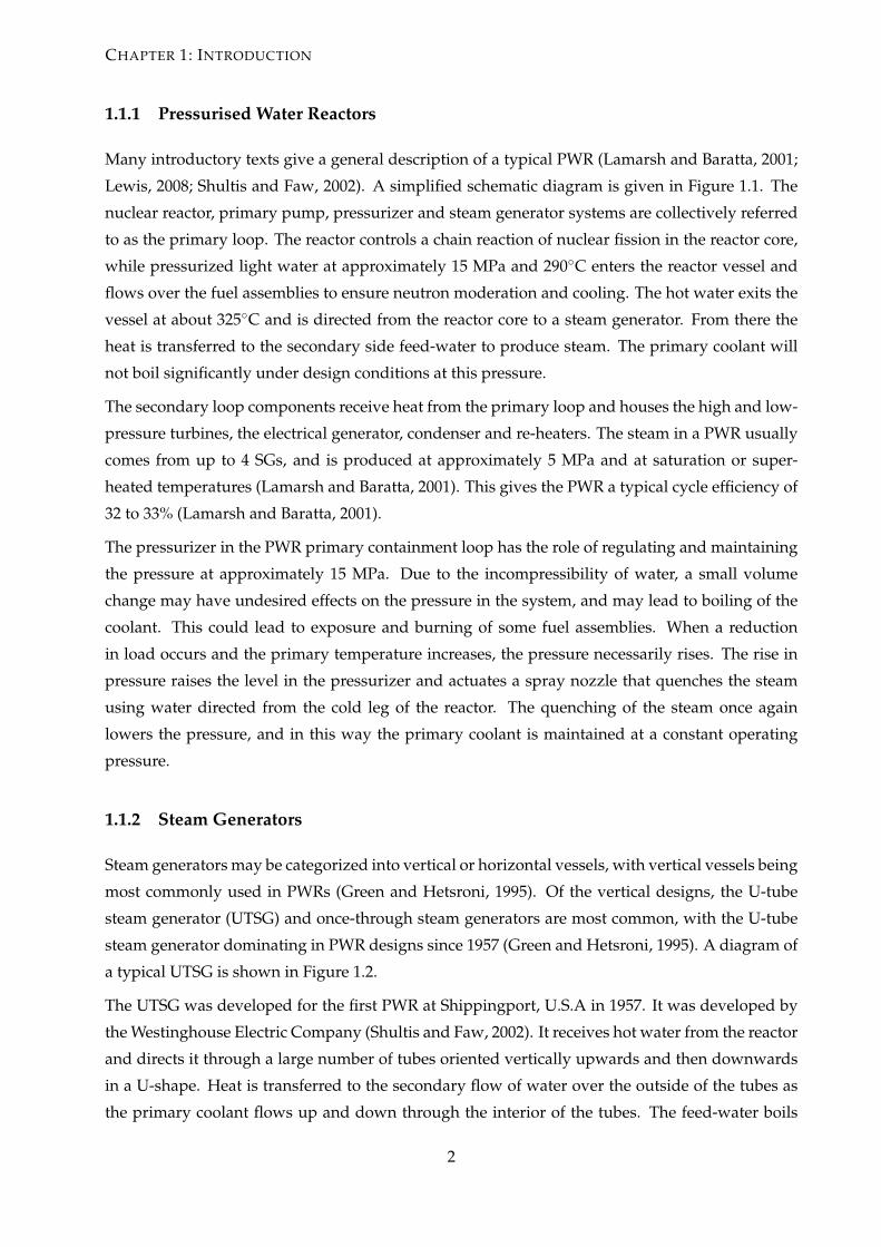
1.1.1 Pressurised Water Reactors
Many introductory texts give a general description of a typical PWR (Lamarsh and Baratta, 2001;
Lewis, 2008; Shultis and Faw, 2002). A simplified schematic diagram is given in Figure 1.1. The
nuclear reactor, primary pump, pressurizer and steam generator systems are collectively referred
to as the primary loop. The reactor controls a chain reaction of nuclear fission in the reactor core,
while pressurized light water at approximately 15 MPa and 290◦C enters the reactor vessel and
flows over the fuel assemblies to ensure neutron moderation and cooling. The hot water exits the
vessel at about 325◦C and is directed from the reactor core to a steam generator. From there the
heat is transferred to the secondary side feed-water to produce steam. The primary coolant will
not boil significantly under design conditions at this pressure.
The secondary loop components receive heat from the primary loop and houses the high and low-
pressure turbines, the electrical generator, condenser and re-heaters. The steam in a PWR usually
comes from up to 4 SGs, and is produced at approximately 5 MPa and at saturation or super-
heated temperatures (Lamarsh and Baratta, 2001). This gives the PWR a typical cycle efficiency of
32 to 33% (Lamarsh and Baratta, 2001).
The pressurizer in the PWR primary containment loop has the role of regulating and maintaining
the pressure at approximately 15 MPa. Due to the incompressibility of water, a small volume
change may have undesired effects on the pressure in the system, and may lead to boiling of the
coolant. This could lead to exposure and burning of some fuel assemblies. When a reduction
in load occurs and the primary temperature increases, the pressure necessarily rises. The rise in
pressure raises the level in the pressurizer and actuates a spray nozzle that quenches the steam
using water directed from the cold leg of the reactor. The quenching of the steam once again
lowers the pressure, and in this way the primary coolant is maintained at a constant operating
pressure.
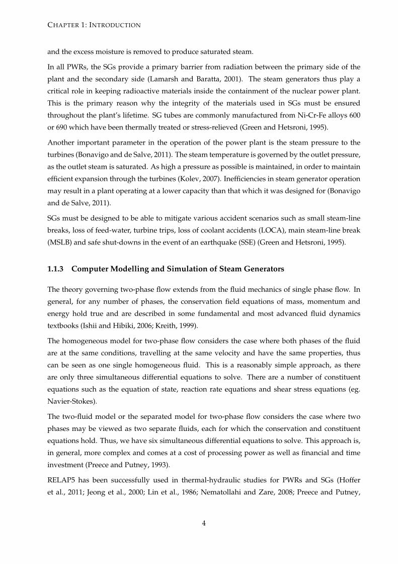
1.1.2 Steam Generators
Steam generators may be categorized into vertical or horizontal vessels, with vertical vessels being
most commonly used in PWRs (Green and Hetsroni, 1995). Of the vertical designs, the U-tube
steam generator (UTSG) and once-through steam generators are most common, with the U-tube
steam generator dominating in PWR designs since 1957 (Green and Hetsroni, 1995). A diagram of
a typical UTSG is shown in Figure 1.2.
The UTSG was developed for the first PWR at Shippingport, U.S.A in 1957. It was developed by
the Westinghouse Electric Company (Shultis and Faw, 2002). It receives hot water from the reactor
and directs it through a large number of tubes oriented vertically upwards and then downwards
in a U-shape. Heat is transferred to the secondary flow of water over the outside of the tubes as
the primary coolant flows up and down through the interior of the tubes. The feed-water boils
2
Page 16
CHAPTER 1: INTRODUCTION
Figure 1.1: Simplified diagram of a PWR connected to the power-producing side of the power
plant (Kok, 2009)
Figure 1.2: Diagram of a typical steam generator used in a PWR (Bonavigo and de Salve, 2011)
3
Page 17
CHAPTER 1: INTRODUCTION
and the excess moisture is removed to produce saturated steam.
In all PWRs, the SGs provide a primary barrier from radiation between the primary side of the
plant and the secondary side (Lamarsh and Baratta, 2001). The steam generators thus play a
critical role in keeping radioactive materials inside the containment of the nuclear power plant.
This is the primary reason why the integrity of the materials used in SGs must be ensured
throughout the plant’s lifetime. SG tubes are commonly manufactured from Ni-Cr-Fe alloys 600
or 690 which have been thermally treated or stress-relieved (Green and Hetsroni, 1995).
Another important parameter in the operation of the power plant is the steam pressure to the
turbines (Bonavigo and de Salve, 2011). The steam temperature is governed by the outlet pressure,
as the outlet steam is saturated. As high a pressure as possible is maintained, in order to maintain
efficient expansion through the turbines (Kolev, 2007). Inefficiencies in steam generator operation
may result in a plant operating at a lower capacity than that which it was designed for (Bonavigo
and de Salve, 2011).
SGs must be designed to be able to mitigate various accident scenarios such as small steam-line
breaks, loss of feed-water, turbine trips, loss of coolant accidents (LOCA), main steam-line break
(MSLB) and safe shut-downs in the event of an earthquake (SSE) (Green and Hetsroni, 1995).
1.1.3 Computer Modelling and Simulation of Steam Generators
The theory governing two-phase flow extends from the fluid mechanics of single phase flow. In
general, for any number of phases, the conservation field equations of mass, momentum and
energy hold true and are described in some fundamental and most advanced fluid dynamics
textbooks (Ishii and Hibiki, 2006; Kreith, 1999).
The homogeneous model for two-phase flow considers the case where both phases of the fluid
are at the same conditions, travelling at the same velocity and have the same properties, thus
can be seen as one single homogeneous fluid. This is a reasonably simple approach, as there
are only three simultaneous differential equations to solve. There are a number of constituent
equations such as the equation of state, reaction rate equations and shear stress equations (eg.
Navier-Stokes).
The two-fluid model or the separated model for two-phase flow considers the case where two
phases may be viewed as two separate fluids, each for which the conservation and constituent
equations hold. Thus, we have six simultaneous differential equations to solve. This approach is,
in general, more complex and comes at a cost of processing power as well as financial and time
investment (Preece and Putney, 1993).
RELAP5 has been successfully used in thermal-hydraulic studies for PWRs and SGs (Hoffer
et al., 2011; Jeong et al., 2000; Lin et al., 1986; Nematollahi and Zare, 2008; Preece and Putney,
4
Page 18
CHAPTER 1: INTRODUCTION
1993; Woods et al., 2009), but has been found to underestimate the secondary side heat-transfer
due to the use of the Chen correlation for the convective heat transfer coefficient during phase
transitions. This results in a lower pressure calculated than expected. The error in the pressure
calculation that is to be expected using RELAP5/mod3 is approximately 0.4 MPa, at a total
pressure of about 5 MPa (Preece and Putney, 1993). Errors may also be expected in the
under-prediction of the liquid inventory on the secondary side, when using RELAP5/mod2. This
error has been partially eliminated with the release of mod3, however, where the introduction of
new inter-phase drag models resulted in an increase in the calculated inventory at full load
conditions (Preece and Putney, 1993).
RELAP5 solves the six field equations of the two-fluid model for two-phase flow, and may use
any of a number of algorithms designed to solve differential equations (such as the implicit or
semi-implicit algorithms).
Flownex has been developed as a systems computational fluid dynamics (CFD) network solver.
It has been validated and verified for use in simulating high temperature gas reactor (HTGR)
technology utilizing a direct Brayton cycle (Greyvenstein and Rousseau, 2003). It has also been
successfully used in gas-turbine combustion modelling (Gouws et al., 2006), as well as many other
industrial applications in two-phase and single-phase flow (Flownex, 2011a,b,c).
Flownex solves the homogeneous field equations, thus inherently being simpler to implement and
achieve convergence of the solution. The graphical user interface of Flownex is also more intuitive
for the end-user than conventional codes from the 1960’s through 1980’s (ie. RELAP5).
1.2 Motivation
Fluid mechanics text books which describe the two-fluid model and the homogeneous model
of two-phase flow do often give criteria and parameters for validity of the use of these models.
Unfortunately, however, the turbulent conditions and the high temperatures and pressures found
in the steam generator are not conducive to accurate modelling (Green and Hetsroni, 1995). It
is extremely difficult to get accurate and consistent measurements from inside the SG, and it is
also very difficult to characterise the foamy emulsion that is the steam/liquid mixture flowing
over the tube bundle. It is therefore not clear and there is certainly a lack of literature describing
how applicable the homogeneous model for two-phase flow is in the context of the nuclear steam
generator performance.
The homogeneous model has a few disadvantages. One loses much of the flow information and
characteristics when reducing the field equations to three from six, or from two-fluids to one. In
many cases, however, this may be acceptable when compared to the subsequent saving of time
and money in the project. The two-fluid model is, on the other hand, a very specific and accurate
5
Page 19
CHAPTER 1: INTRODUCTION
way of modelling the flow of two-phases. It takes into account drag between the phases as well as
momentum, energy and mass transfer between the phases. Of course, with an increase in accuracy
there is a drastic increase in complexity of the model. It will require increased processing power,
and the software is considerably more expensive.
It would therefore certainly be advantageous to the plant or component engineer to know when
it may be suitable to make use of more financially sound resources and when it would necessitate
a higher expenditure in time or money. Currently, the cost of participating in the development
of complex steam generator simulation programs such as ATHOS (Singhal et al., 1984) and Triton
(SG software from the Electric Power Research Institute) runs upwards of R1 million a year with
a five year commitment.
Flownex is developed locally, and comes at a considerably lower price than competitor software,
and is also more user friendly.
There are thus clear advantages and disadvantages to using either code-base, but very little
guidance for the engineer to decide which software is more suitable.
1.3 Problem Statement
Issues with steam generators result in large annual monetary losses for utility companies world-
wide. There are currently large amounts of uncertainties inherent in steam generator models. The
turbulent and chaotic conditions in the SG make it difficult to accurately model and predict flow
parameters.
There is little literature to describe conditions under which the various models are applicable. It is
clear that when the phenomenon of boiling must be considered in-depth, that the homogeneous
model will not be sufficient. It remains unclear, however, under which specific conditions it is
acceptable to use the homogeneous model over the two-fluid model.
This study assesses the differences in the two models within the context of nuclear steam
generators. It attempts to find at which conditions certain parameters show large variance
between the models. It also aims to provide direction in the selection of the model type when
performing SG analysis.
1.4 Methodology
Often, in modelling two-phase flow, the problem is simplified so that important features of the
flow are retained and analysis is still meaningful (Kok, 2009).
The research methodology followed in this study is quantitative, in the form of model
6
Page 20
CHAPTER 1: INTRODUCTION
Data from
Koeberg
NPP
Literature
Survey
Data
compilation
Simplification
of geometry
Coding and
set-up of
models
Analyse results
and give
recommendations
Steady-state
calculation
Development
Evaluation
Validation
against plant
operating
data
Figure 1.3: Quantitative research methodology with model development
development and evaluation.
Specifications of a PWR steam generator obtained from Koeberg Nuclear Power Plant form the
basis of the models. The models are verified with a steady-state calculation in EES. The primary
conditions are obtained from this calculation as there was no primary data supplied by Koeberg.
The verification ensures simple mathematical consistency between the input and output
conditions. It is not feasible to re-write the fluid models for verification purposes, as RELAP5 has
been verified in previous studies (RELAP5, 2001d).
Validation is done against secondary side operating data supplied by Koeberg. The results from
the RELAP5 and Flownex models are tabulated and the deviation from the plant data is recorded.
The results form a set of comparisons in graphic form between the two models at various power
levels. This provides a sound basis for making recommendations on further improvements and
future extensions to the model. The research methodology is summarised in Figure 1.3.
7
Page 21
CHAPTER 2
Overview of the Literature
2.1 Issues facing Steam Generator operators
A major issue with steam generator operation is the degradation of materials used in its
construction (Bonavigo and de Salve, 2011).
Uranium, trans-uranium elements and fission products may occur in the primary coolant and
are caused by defects in the fuel rod cladding. They may also result from free uranium particles
in the coolant also under-going fission (Bonavigo and de Salve, 2011). Corrosion products from
the shell, tube and support structures may also contaminate primary or secondary water. These
conditions increase the need for inspection, cleaning, maintenance and safe decommissioning of
any particular SG.
For this reason, it is important to monitor and model carry-over of liquid by the SG, as damage
to the turbine may have severe consequences for the plant (Bonavigo and de Salve, 2011). It is
also useful to include solid accumulation and chemical reactions in the model of the SG, as the
quality and chemical parameters of the water (such as pH, Boric Acid concentration, Chlorides
concentration, Impurity content and dissolved Oxygen) play a large role in degradation (Bonavigo
and de Salve, 2011).
2.1.1 Degradation of the primary side
Some of the degradation that has been observed in the primary side of SGs are (Diercks et al.,
1999; Green and Hetsroni, 1995; Riznic, 2009; Schwarz, 2001):
• Stress corrosion cracking and inter-granular attack.
• Tube plugging.
• Tube denting.
8
Page 22
CHAPTER 2: OVERVIEW OF THE LITERATURE
• Flow-induced vibrations.
• Tube leakage.
• Tube support fretting.
2.1.2 Degradation of the secondary side
For the secondary side, some examples of degradation include (Bonavigo and de Salve, 2011;
Schwarz, 2001) :
• Tube support degradation.
• Tube fouling (build up of magnetite on the outside of the tubes resulting in lower thermal
efficiency).
• Secondary side deposits and sludge build-up.
These issues occur primarily in steam generators which formed part of the original fleet (of which
Koeberg is one) where Alloy 600 MA (Ni-Cr-Fe) is used for the construction of the primary tubes.
In newer steam generators, Alloy 600 TT, Alloy 690 TT and Alloy 800 (containing less Ni-Cr-Fe
with small concentrations of Al and Ti) tubes have performed better. These newer materials have
not mitigated the issues completely (EPRI, 2012b).
2.1.3 The cost effect of degradation
It is estimated by Electric Power Research Institute (EPRI) (EPRI, 2012b) that a tube rupture or
leakage may cost the utility between R40 million and R150 million per event1. The large variance
in the number is due to the wide range of issues which may lead to component replacement
and shut-down of the power plant. Integrity and performance assessments of steam generators
may cost between R7 million and R14 million2. Approximately 75% of steam generator outages
are caused by degradation and corrosion in the tubes (Millett and Welty, 2010). Steam generator
research is, therefore, extremely valuable and critical to the safe and cost effective operation of
nuclear power plants.
2.1.4 The effect of degradation on heat transfer and efficiency
Chemical treatment of the primary side results in a mostly corrosion resistant environment,
although degradation does occur on the primary side in small amounts. It is thus the
1$5-$15 million in March 20122$1-$2 million in March 2012
9
Page 23
CHAPTER 2: OVERVIEW OF THE LITERATURE
feed-water/steam cycle (secondary side), which contributes largely to the degradation in heat
transfer performance (Schwarz, 2001). The drop in heat transfer efficiency due to the
accumulation of solids or degradation of the tubes and shell is characterized by the fouling factor
(R f ). The effect of the fouling factor can be seen if we examine how the over-all heat transfer
coefficient is calculated, in Equation 2.1.1.
1U
=do
di
1hi
+do
2kwln
do
di+
1ho
+ R f (2.1.1)
The fouling factor is the heat transfer resistance, or inverse heat transfer coefficient, for the build
up of solids found in the secondary side. Fouling factors are measured experimentally, and typical
ranges are found to be (Schwarz, 2001):
(δR f
δTin) = +0.11... + 0.13
10−5m2K/WK
(δR f
δTout) = +0.6... + 0.6
10−5m2K/WK
(δR f
δpst) = −0.7...− 1.2
10−5m2K/Wbar
From the above equations, we note that a typical fouling factor varies roughly 0.10 m2K/WK with
variation of inlet temperature. The heat transfer coefficient is inversely proportional to the heat
resistance, so this creates uncertainty in the heat transfer coefficient by up to a factor of 10. If a
typical heat transfer coefficient is in the order of 20 000 Wm2K , then it may be reported in the model
as low as 18000 or as high as 22000, purely as an effect of the fouling factor alone. Of course, the
degradation issue is complex and much larger discrepancies in calculated heat transfer coefficients
are expected.
2.1.5 Concluding remarks regarding issues faced in steam generator operation
From the above discussion, it is clear that there exists a need in the industry and in academia to
study the effects of steam generator performance. To this end, studies focus largely on utilizing
mathematical models of the two-phase flow regions of the steam generator. For many of the
complex issues where interactions of particles within the fluid affect deposition and degradation
of the tubes, it is necessary to employ techniques such as computational fluid dynamics (CFD)
and discrete element analysis (DEM) coupled with models of chemical reactions. These
techniques allow detailed analysis of the problem, and may be utilized to aid in the design of
new components. They are time consuming and involve complex and expensive software,
however, and are thus not always suitable for operational analysis of general plant performance
conditions.
10
Page 24
CHAPTER 2: OVERVIEW OF THE LITERATURE
The flow solvers such as Flownex and RELAP5 (Sections 2.3.1 and 2.3.2) allow an arbitrary amount
of detail in the modelling of flow paths in the form of nodes and components, but one is restricted
to the components offered by the individual modelling package. RELAP5 and Flownex allow one
to construct flow paths for all the components in the nuclear power plant, and a network of pipes
is used to model the steam generator. This allows for a detailed operational analysis. If a fine
enough nodalization is used, then a large amount of detailed flow analysis may be obtained at
specific points in the steam generator.
2.2 Thermal-fluid models of two-phase flow
The subject of multiphase flow has become increasingly important since the inception of nuclear
power, as it occurs in many of the primary components of the nuclear power plant. In the PWR,
the primary coolant is kept sub–cooled at a high pressure and thus remains in a single phase. The
secondary water on the shell-side of the steam generator is heated from sub-cooled to saturated,
undergoing evaporation. A combination of forced and boiling convective conditions in the
two-phase mixture results in extremely turbulent flow conditions within the shell-side. The
correlations used to predict two-phase thermal-hydraulic parameters are thus less accurate and
not as well understood as those for single-phase flow (Ishii and Hibiki, 2006).
For single-phase flow, the model is formulated from continuum mechanics in terms of the field
equations for conservation of mass, energy and momentum. The field equations are then
complemented by various constituent equations which describe thermodynamic state, energy
transfer and chemical reactions.
2.2.1 Multi-phase flow and phase transitions
There are, in general, three models used to describe two-phase flow of a fluid, namely the
homogeneous model, the drift-flux model and the two-fluids model (Ishii and Hibiki, 2006).
They are formulated in terms of the field equations for the conservation of mass, energy and
momentum; similarly to the single-phase model. Complications arise from the fact that there are
two separate fluids being modelled (liquid and vapour) and they are subject to multiple,
deformable and movable interfaces between the two phases. Furthermore, there exists mass and
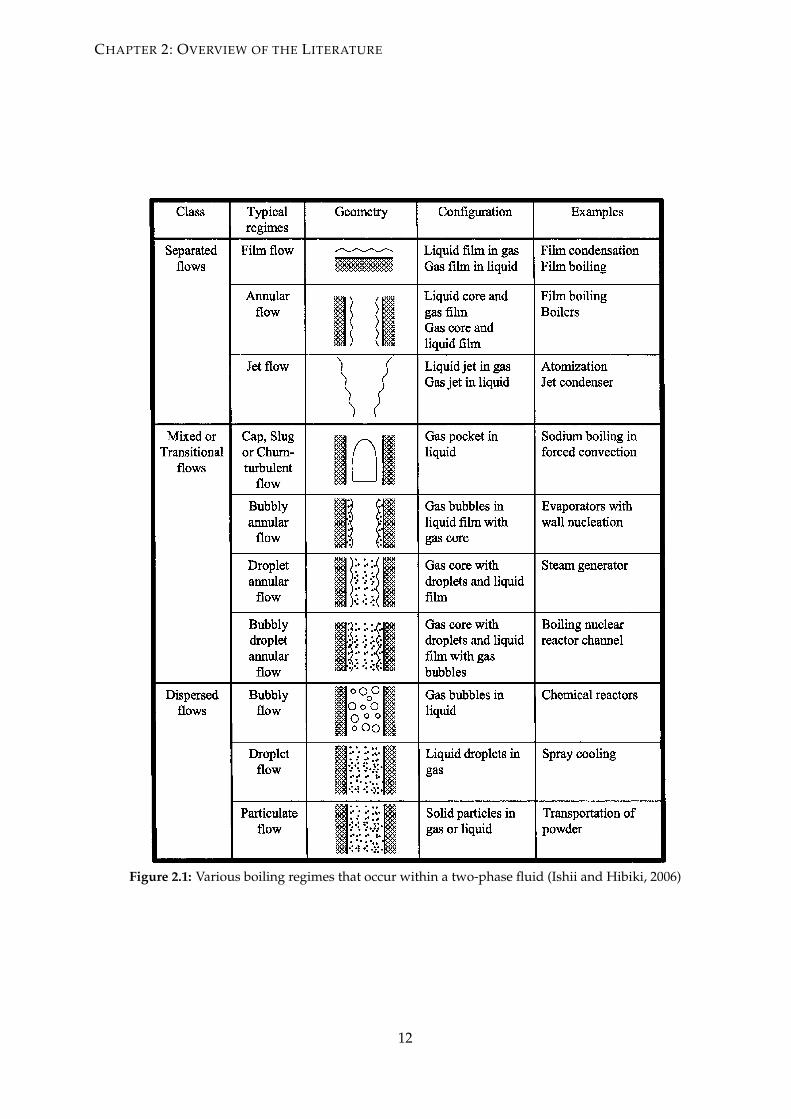
energy transfer across these interfaces. This gives rise to the various boiling flow regimes that
occur in vertical pipes, shown in Figure 2.1.
The flow through the secondary side of the steam generator generally falls within the mixed flow
class where the gas contains entrained liquid, and the liquid contains entrained gas. The interfaces
in these regimes are rapidly changing form and size, and therefore an accurate model based on
physical principals is virtually impossible (Ishii and Hibiki, 2006).
11
Page 25
CHAPTER 2: OVERVIEW OF THE LITERATURE
Figure 2.1: Various boiling regimes that occur within a two-phase fluid (Ishii and Hibiki, 2006)
12
Page 26
CHAPTER 2: OVERVIEW OF THE LITERATURE
Figure 2.2: Flow regime matrix for vertical flow used in RELAP5 for boiling heat transfer
calculations (RELAP5, 2001c)
Software packages such as RELAP5 have been coded with complex boiling flow regime and
boiling heat transfer regime matrices. Figure 2.2 shows how RELAP5 uses the average mixture
velocity (vm) and the average void fraction (αg) to assess which flow regime best characterizes the
flow. The RELAP5 documentation (RELAP5, 2001b) describes the models and correlations in
finer detail. These flow regimes dictate which correlations are used in inter-phase drag and shear,
wall friction, heat transfer and inter-phase heat and mass transfer (RELAP5, 2001b).
Figure 2.3 illustrates the boiling curve employed by RELAP5 to calculate heat flux during fluid-
to-wall heat transfer (RELAP5, 2001b).
As the physics change during phase transitions, so does the correlation required to calculate the
heat flux. Table 2.1 shows an example of which correlations are used by RELAP5 to calculate heat
flux for each boiling regime. The RELAP5 documentation (RELAP5, 2001b) expands further on
each correlation. The Chen correlation is applied during nucleate boiling and transition boiling,
and thus makes up the majority of the boiling regime which occurs during nominal SG operation.
This is because all effort goes to operating the steam generator below or near the critical heat flux,
within the nucleate or transition boiling regime (as seen in Figure 2.3).
Table 2.1: Heat transfer correlations used in the various boiling regimes for RELAP5Boiling regime
Laminar Natural Turbulent Condensation Nucleate boiling Transition boiling Film boiling CHF
Heat transfer correlation Sullars, Nu = 4.36 C-Chu or McAdams Dittus-Boelter Nusselt/Chato-Shah-Coburn-Hougen Chen Chen Bromley Table
In Flownex, the Steiner and Taborek correlation is natively used to calculate the boiling heat
transfer coefficient during nucleate boiling, while the Berenson correlation is applied during
transition boiling.
13
Page 27
CHAPTER 2: OVERVIEW OF THE LITERATURE
Figure 2.3: The boiling and condensing curve used by RELAP5 to calculate heat flux (RELAP5,
2001b)
Table 2.2: Heat transfer correlations used in the various boiling regimes for FlownexBoiling regime
Laminar Natural Turbulent Condensation Nucleate boiling Transition boiling Film boiling CHF
Heat transfer correlation Dittus-Boelter Steiner and Taborek Berenson Zuber Table
The mathematical details for the correlations may be found in various texts (Flownex, 2011b;
Janna, 2000; RELAP5, 2001b; Rohsenow et al., 1998; Thome, 2004). None of the correlations by
themselves offer an accurate solution to the boiling heat transfer problem, and it would not
benefit the study to go further into each correlation. When they are combined and used in matrix
form such as RELAP5 does, it increases the accuracy of the solutions substantially over using a
single correlation. It is important to note the amount of effort required to perform such
calculations in one’s own code, and to keep the scope of the project in context.
2.2.2 Chen correlation for the nucleate boiling heat transfer coefficient
In order to directly compare the homogeneous two-phase flow model with the two-fluid model
without introducing error due to different heat transfer correlations, it is necessary to perform
the calculation using the same correlations in both models. The nucleate and transition boiling
regions of the steam generator are much larger than the super-heated sections, and thus play the
largest role in affecting the heat transfer of the system (Green and Hetsroni, 1995).
RELAP5 applies the Chen correlation to both the nucleate and transition boiling regime, and thus
it will be discussed briefly. It is not possible to alter the correlations that RELAP5 uses, however,
we are able to alter what Flownex uses. Therefore, it was decided to modify Flownex to use the
14
Page 28
CHAPTER 2: OVERVIEW OF THE LITERATURE
Chen correlation during nucleate and transition boiling, as opposed to the Steinberg and Tamorek
correlation already present.
Formulation
Chen’s correlation states that the local two-phase boiling coefficient is made up of two parts from
the nucleate boiling regime and the convective (single-phase) regime (Thome, 2004).
htp = hnb + hcb (2.2.1)
He further determined that the nucleate boiling coefficient and the convective coefficient could be
calculated by older correlations and adjusted by a multiplying factor.
htp = hFZ × S + hL × F (2.2.2)
The equation of Forster and Zuber is used to calculate the coefficient for nucleate boiling.
hFZ = 0.00122[k0.79
L c0.45pL ρ0.49
L
σ0.5µ0.29L h0.24
LG ρ0.24G
]× ∆T0.24sat × ∆p0.75
sat (2.2.3)
Where ∆Tsat = Twall − Tsat and ∆psat = pwall − psat.
The convective heat transfer coefficient is calculated by the Dittus-Boelter correlation.
hL = 0.023Re0.8L Pr0.4
L [kL
di] (2.2.4)
It is important to note that the Reynoulds number used in the Dittus-Boelter correlation is the
single-phase liquid Reynould’s number.
ReL =m(1− x)di
µL(2.2.5)
Where x is the quality of the flow. PrL is the liquid Prandtl number.
PrL =cpLµL
kL(2.2.6)
The multipliers for the Chen correlation are:
F = (1
Xtt+ 0.213)0.736 (2.2.7)
Xtt = (1− x
x)0.9(
ρG
ρL)0.5(
µL
µG)0.1 (2.2.8)
S =1
1 + 0.00000253Re1.17tp
(2.2.9)
And finally, the two-phase Reynould’s number is also calculated with a multiplier.
Ret p = ReL × F1.25 (2.2.10)
15
Page 29
CHAPTER 2: OVERVIEW OF THE LITERATURE
Application
Chen’s correlation is widely applicable, including water in upward and downward flow and
pressures from 0.55 to 34.8 bar. It is valid mostly between qualities of 0.01 and 0.71, but has been
shown to be accurate beyond this range as well (Thome, 2004). Typically, an iterative calculation
is performed between Twall and pwall , if the heat flux is specified. It applies only while the wall
remains wet, and thus reduces in accuracy as the boiling regime shifts to film boiling.
In this study, the focus is on the steady-state operation of the steam generator at nominal
conditions, and thus we assume that most of the flow will be occurring within the nucleate
boiling regime as predicted by Green and Hetsroni (1995). Thus the modification of Flownex to
use the Chen correlation is justified.
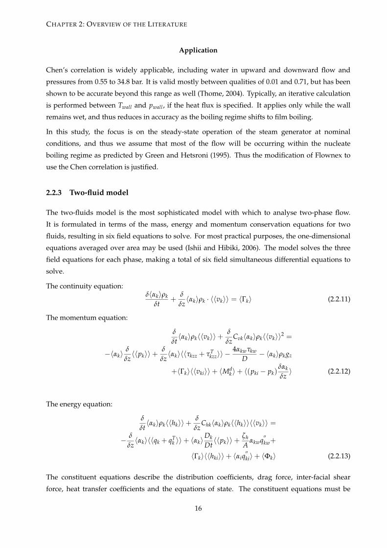
2.2.3 Two-fluid model
The two-fluids model is the most sophisticated model with which to analyse two-phase flow.
It is formulated in terms of the mass, energy and momentum conservation equations for two
fluids, resulting in six field equations to solve. For most practical purposes, the one-dimensional
equations averaged over area may be used (Ishii and Hibiki, 2006). The model solves the three
field equations for each phase, making a total of six field simultaneous differential equations to
solve.
The continuity equation:δ〈αk〉ρk
δt+
δ
δz〈αk〉ρk · 〈〈vk〉〉 = 〈Γk〉 (2.2.11)
The momentum equation:
δ
δt〈αk〉ρk〈〈vk〉〉+
δ
δzCvk〈αk〉ρk〈〈vk〉〉2 =
−〈αk〉δ
δz〈〈pk〉〉+
δ
δz〈αk〉〈〈τkzz + τT
kzz〉〉 −4αkwτkw
D− 〈αk〉ρkgz
+〈Γk〉〈〈vki〉〉+ 〈Mdk 〉+ 〈(pki − pk)
δαk
δz〉 (2.2.12)
The energy equation:
δ
δt〈αk〉ρk〈〈hk〉〉+
δ
δzChk〈αk〉ρk〈〈hk〉〉〈〈vk〉〉 =
− δ
δz〈αk〉〈〈qk + qT
k 〉〉+ 〈αk〉Dk
Dt〈〈pk〉〉+
ζh
Aαkwq
′′kw+
〈Γk〉〈〈hki〉〉+ 〈αiq′′ki〉+ 〈Φk〉 (2.2.13)
The constituent equations describe the distribution coefficients, drag force, inter-facial shear
force, heat transfer coefficients and the equations of state. The constituent equations must be
16
Page 30
CHAPTER 2: OVERVIEW OF THE LITERATURE
chosen very carefully, otherwise the model will not accurately describe certain flow
characteristics. Detailed information on the two-fluid model is found in many thermal-fluid
texts, including Ishii and Hibiki (2006).
2.2.4 Homogeneous model
A rather simplified way of analysing two-phase flow arises with the homogeneous flow model.
In this model, the inter-facial energy and momentum transfer as well as the inter-phase velocities
are neglected. The six field equations from Section 2.2 can be reduced to four field equations. The
mass, energy and momentum equations are written in terms of a homogeneous mixture of the two
phases, while the mass equation for the gas phase is still included as to take into account thermal
non-equilibrium between the two phases (Ishii and Hibiki, 2006).
The mixture mass equation:ρm
t+
δ
δz(ρmvm) = 0 (2.2.14)
The vapour phase concentration (mass) equation:
δα2 ¯ρ2
δt+
δ
δz(α2 ¯ρ2vm) = Γk (2.2.15)
The momentum equation:
δρmvm
δt+
δ
δz(ρmvmvm) = −
δpm
δz+
δ
δz(Σ + ΣT) + ρmgm + Mm (2.2.16)
The energy equation:
ρmim
δt+
δ
δz(ρmimvm) = −
δ
δz(q + qT) +
Dpm
Dt+ Φµ
m + Φσm (2.2.17)
The constituent equations are used to solve for stress tensors and heat flux, among other
parameters.
By assuming a homogeneous mixture, we are assuming that the relative velocity between the two
phases is zero. The stress tensors are written in terms of the viscosity of the fluids, and the heat
fluxes are written in terms of the heat transfer coefficients. There are thus fewer equations to solve
and fewer constituent equations to append to the model.
The homogeneous model is typically reserved for simple problems where accuracy of the SG
interior is not of prime importance. Instead, focus is on the causal relationships between input and
output variables (Green and Hetsroni, 1995). The model is generally not applicable when the flow
is drag-dominated under the effect of gravity. An example is in vapour bubbles rising through
liquid water, where the body forces (gravity and buoyancy) balances against the inter-phase drag
(EPRI, 2012a). This may be applicable to a steam generator under low power conditions.
17
Page 31
CHAPTER 2: OVERVIEW OF THE LITERATURE
Seperator
Secondaryout
Primary
in
Primary
out
Secondaryin
Figure 2.4: Typical nodalization for the model of a steam generator
2.3 Simulating steam generators using thermal-hydraulic codes
Thermal-hydraulic codes generally provide input in the form of component models. Pipes,
reservoirs, accumulators, fluid volumes, annuli, valves, moisture separators, pumps and turbines
all are types of components that that may be specified as part of the model. General geometrical
properties such as hydraulic diameter, length, volume, flow area and changes in height may be
specified for each component. Furthermore, heat transfer elements may also be specified to
simulate the heat transfer between the primary and secondary side models. Boundary conditions
such as temperature and pressure of feed-water and primary coolant as well as mass flows
should also be specified (Green and Hetsroni, 1995).
Important parameters for a typical thermal-hydraulic model of a steam generator can be expressed
with the components as shown in Figure 2.4. This type of diagram is referred to as the nodalization
of the model.
For steady-state calculations, the following boundary conditions may be specified (Singhal et al.,
1984):
18
Page 32
CHAPTER 2: OVERVIEW OF THE LITERATURE
• Mass flow-rate of primary coolant through the SG, mp.
• Mass flow-rate of feed-water added into the down-comer, m f d.
• Inlet temperature of the feed-water, Tf d.
• Mass quality of steam leaving the dome, xs.
• Mass fraction of steam entrained in the recirculating water flowing from the dome to the
down-comer, xw.
• Pressure in steam dome, pd.
• Height of the water level in the down-comer, hWL.
• Fraction of the down-comer feed-water added to the hot side, fdh (this implies that the
fraction [1 - fdh] is added on the cold side).
The resulting parameters should show local flow conditions such as temperature, pressure,
velocity, quality and void fraction of both phases as well as the following global parameters
(Singhal et al., 1984) :
• Circulation ratio, defined as Total mass flow-rate through the boiler regionMass flow-rate of liquid recirculated from the steam separators .
• Liquid inventory in the tube bundle and riser section.
• Liquid inventory in the down-comer.
• Temperature of the down-comer water at the entry to the tube bundle region.
• In transient calculations, the primary inlet temperature is generally described as a function
of time, and the primary outlet temperature and heat load are calculated as a function of
time.
2.3.1 Flownex
Flownex software research began in 1986 and was initially designed to solve air distribution
networks. It was subsequently expanded by M-Tech Industrial Pty (Ltd) and in 1999, M-Tech was
contracted to perform studies on the pebble-bed modular reactor (PBMR) using Flownex. In
2007, the National Nuclear Regulator (NNR) reviewed the Flownex verification and validation
status and found it to be acceptable for use in the support and design of safety issues in the
PBMR. Flownex was expanded and integrated into the Simulation Environment (Flownex SE) in
2008. From this they formed a package for comprehensive plant simulation, analysis and
optimization (Flownex, 2011c). This is the form it is used in today, and it allows one to model any
19
Page 33
CHAPTER 2: OVERVIEW OF THE LITERATURE
network of pipes, pumps and heaters. This is shown in the nodalization for the SG in Figure 2.4.
Flownex solves the field equations using an Implicit Pressure Correction Method (IPCM)
(Flownex, 2011b). The software has various advantages and disadvantages, described in Table
2.3.
Table 2.3: Advantages and Disadvantages to using Flownex and the homogeneous model.
Advantages Disadvantages
Simple formulation Not useful for accurate modelling of internal flow parameters
Simple computability Software not widely used in nuclear industry
Quick model development process Homogeneous assumption limitations
Inexpensive, local software
Stable
Approved by NNR for use in PBMR studies
Real-time solving of transients
2.3.2 RELAP5/Mod3.4
The RELAP5 code was developed for best-estimate steady-state and transient simulation of light
water reactor coolant systems during normal operation as well as accident scenarios (RELAP5,
2001a). It was developed for the NRC in conjunction with many other countries and research
organisations, and most of the development took place at Idaho National Engineering
Laboratory. The code is based on the non-homogeneous, non-equilibrium model for two-phase
flow and includes many component models from which systems can be built. It is able to model
pumps, valves, pipes, heat structures, reactor point kinetics, special fluid process models (such as
jet pumps and choking), turbines and separators. It makes use of a partially implicit numerical
solving scheme which is fast to solve, however only accurately predicts first-order effects
(RELAP5, 2001a). As with Flownex, small time steps must be used to preserve accuracy but the
solution is generally stable over most conditions (Preece and Putney, 1993).
Table 2.4: Advantages and Disadvantages to using RELAP5 and the two-fluid model.
Advantages Disadvantages
Supported by the US NRC Expensive, proprietary software
Accurately model internal flow paths Complicated model development
Improved accuracy Longer solving time
Large body of knowledge and experience
Stable
20
Page 34
CHAPTER 2: OVERVIEW OF THE LITERATURE
2.3.3 Previous work on steam generator models
A comparison between steam generator models using the homogeneous model and the two-fluid
model was done in 1980 (Singhal et al., 1980). They used a finite difference method to solve the
field equations, and the results concluded that there were significant differences both in local and
global flow parameters predicted by the two models. There was, however, no experimental or
operational data to compare either model to. The computational advances since 1980 mean that
the results of this study may not be applicable any more, but it does offer an indication that there
will be significant differences in the parameters predicted by the two models.
RELAP5 and the two-fluid model has been used successfully in many simulations of PWRs and
their components (Colorado et al., 2011; Hoffer et al., 2011; Jeong et al., 2000). The RELAP5 models
were, in all cases, using the two-fluid model. From these studies, it is found that it is not necessary
to have more than five increments in the down-comer and riser component models for a simple
model. Five increments have been shown to be sufficient to model all important flow parameters
in the riser and down-comer regions (RELAP5, 2001c). It is also shown that it is necessary to model
the recirculation from the moisture separation, as it has a large impact on the natural circulation
through the system (Green and Hetsroni, 1995; Jeong et al., 2000). It also becomes apparent that
the choice of the convective heat transfer coefficient correlation affects the calculated heat transfer
greatly. RELAP5/Mod3.4 uses the Chen correlation described in detail in Thome (2004). It relates
the total convective heat transfer coefficient to a weighted linear summation of the single-phase
convective heat transfer coefficient and the coefficient for nucleate boiling. The coefficients are
weighted by a nucleate boiling suppression factor and a two-phase multiplier. It must be noted
that the Chen correlation is, in general, only valid for plain vertical tubes. Due to it’s simplicity,
however, it is still commonly used in many simulation models (Colorado et al., 2011; Hoffer et al.,
2011; Jeong et al., 2000; Lin et al., 1986).
The use of the Chen correlation in RELAP5 results in an under-prediction of SG heat transfer for
the majority of load conditions ranging from 36% to 100% (Preece and Putney, 1993). The exiting
steam is saturated, therefore, the error in heat-transfer relates directly to the error in the outlet
steam pressure. The error reported was lower at low power, but at full load is approximately 0.4
MPa. The under-prediction of the heat transfer results in a lower steam pressure than expected.
The inter-phase drag force is also over-predicted with RELAP5/Mod3 and can contain an error of
up to 25% (Preece and Putney, 1993).
The homogeneous model is commonly used when comparing codes that do not include the two-
fluid model, such as older versions of ATHOS and computational fluid dynamics (CFD) packages.
CFD analysis of homogeneous mixture flow is still useful, as velocity profiles and temperature
distributions may still be determined (EPRI, 2012a). The homogeneous model is also applicable at
low power loads such as hot shut-downs, when the reactor is shut down but still operating under
decay heat (EPRI, 2012a).
21
Page 35
CHAPTER 3
Basis for the Models
One of the goals of the project was to develop a steady-state thermodynamic model for the u-
tube steam generator. The software that was chosen for the model development was RELAP5
and Flownex in order to facilitate a direct comparison between the two-fluid and homogeneous
model.
RELAP5 was chosen to perform two-fluid analysis due to it being widely used in the nuclear
industry, well supported, well documented, and already licensed for use at the North-West
University.
Flownex was chosen to perform additional homogeneous analysis due to it being widely used in
South Africa in the power generation and fluid modelling industries. It is also well supported and
licensed at the North-West University.
The steam generator that was modelled was a Westinghouse Type 51B u-tube steam generator.
Data from Koeberg NPP was used to validate the models; this is discussed in the next section.
3.1 Data obtained from Koeberg Nuclear Power Station
The steady-state data was obtained from Koeberg NPP, and a sample is shown in Table 3.1. The
data consists of tables of values for the primary inlet and outlet temperatures, the pressure in
the steam drum, the feed-water pressure and temperature, the feed-water and steam flow-rate
and the active power produced by the generator. These variables make up the typical boundary
conditions of the steam generator model. As there was no detailed data of the internal flow of the
steam generator, the model was validated against these boundary conditions.
The data was taken from selected points throughout the plant, and was requested once a day at
midday. In total, there was roughly 10 years of steady-state data. There are null and erroneous
values scattered throughout, as well as weeks when the reactor was being ramped up or ramped
down. It was thus difficult to obtain enough data points at various steady-state conditions. It
22
Page 36
CHAPTER 3: BASIS FOR THE MODELS
Tabl
e3.
1:Sa
mpl
eof
the
stea
dy-s
tate
data
obta
ined
from
asi
ngle
unit
atK
oebe
rgN
ucle
arPo
wer
Stat
ion
Dat
eT h
ot(◦
C)
T col
d(◦ C
)SG
drum
pres
sure
(kPa
)Fe
ed-w
ater
pres
sure
(kPa
)Fe
ed-w
ater
tem
pera
ture
(◦C)
Feed
-wat
erflo
w-r
ate(k
g/s)
Stea
mflo
w-r
ate
(kg/
s)G
ener
ator
acti
vepo
wer
(MW
)
2000
/01/
0112
:00
303.
034
280.
299
5495
.419
5714
.844
198.
848
1094
.096
1142
.277
600.
365
2000
/01/
0212
:00
302.
714
280.
256
5492
.824
5717
.285
198.
699
1095
.571
1139
.469
602.
197
2000
/01/
0312
:00
302.
927
280.
449
5508
.393
5729
.492
198.
692
1097
.045
1144
.384
605.
860
2000
/01/
0412
:00
312.
778
278.
654
4916
.817
(nul
l)22
0.04
817
75.5
4118
51.3
7495
3.47
9
2000
/01/
0512
:00
312.
201
278.
547
4911
.628
(nul
l)22
0.10
917
85.0
6418
45.7
5794
8.71
7
2000
/01/
0612
:00
(nul
l)(n
ull)
(nul
l)(n
ull)
(nul
l)(n
ull)
(nul
l)(n
ull)
2000
/01/
0712
:00
312.
329
278.
568
4919
.412
5307
.129
220.
222
1816
.892
1855
.586
952.
013
2000
/01/
0812
:00
312.
885
278.
632
4919
.412
(nul
l)22
0.25
117
87.3
2618
56.9
9095
2.38
0
2000
/01/
0912
:00
312.
692
278.
825
4937
.574
(nul
l)22
0.26
317
93.6
3718
56.9
9095
1.64
7
2000
/01/
1012
:00
312.
756
278.
675
4924
.602
(nul
l)22
0.25
117
80.5
3618
56.2
8894
8.35
0
2000
/01/
1112
:00
312.
628
278.
483
4909
.033
5314
.453
220.
299
1791
.385
1853
.480
947.
618
2000
/01/
1212
:00
312.
414
278.
654
4919
.412
(nul
l)22
0.04
118
11.5
5318
56.2
8894
8.71
7
2000
/01/
1312
:00
312.
692
278.
675
4924
.602
(nul
l)22
0.21
917
99.4
8018
54.8
8495
0.91
5
2000
/01/
1412
:00
312.
329
278.
333
4898
.655
5294
.922
220.
183
1803
.066
1847
.161
950.
182
2000
/01/
1512
:00
312.
863
278.
782
4924
.602
5321
.777
220.
183
1811
.553
1847
.863
952.
380
2000
/01/
1612
:00
312.
607
278.
590
4919
.412
5314
.453
220.
195
1798
.131
1853
.480
949.
449
2000
/01/
1712
:00
312.
350
278.
611
4911
.628
(nul
l)22
0.18
317
90.9
3318
45.7
5795
4.94
4
2000
/01/
1812
:00
312.
543
278.
697
4911
.628
(nul
l)22
0.25
517
94.9
8918
51.3
7495
2.38
0
2000
/01/
1912
:00
312.
628
278.
504
4903
.845
(nul
l)22
0.31
518
03.5
1218
56.2
8895
1.28
1
23
Page 37
CHAPTER 3: BASIS FOR THE MODELS
was for this reason that only power outputs of 100%, 80% and 60% were evaluated in this project.
There were not enough reliable data points at low power conditions for a reliable analysis.
The data was sorted by power from the generator as to group data points with similar values.
The data entries with null values were discarded from the set. All data points that corresponded
to 100%, 80% and 60% respectively were separated and made up in new datasets for each power
level. The Statistical Analysis Tool in Microsoft Excel was then used to analyse the datasets. The
results are discussed in the next section.
3.1.1 Statistical analysis of the data
The results of the statistical analysis for the data at 100%, 80% and 60% power output are given
in Table 3.2, Table 3.3 and Table 3.4 respectively. The important parameters to note are the mean
and the confidence level at 95%. The confidence level may be understood by Equation 3.1.1. For
example, with a mean of 270.342 reported and a confidence level (at 95%) of 4.756, the mean is
read as in the example below.
µ = 270.342± 4.756 (3.1.1)
Equation 3.1.1 means that 95% of the data points in our analysis fall within the stated interval.
Kurtosis refers to the peak of a probability distribution when compared with a normal
distribution. A higher kurtosis indicates a higher peak, with more of the data concentrated
around the mean than the shoulders of the distribution (Dodge, 2003).
The skewness of a distribution refers to where the majority of data points are concentrated. A
negative skewness means that more of the data points are found to the right of the mean, while a
positive skewness means the opposite. The skewness could indicate whether there are a number
of outliers in the data. A large negative skewness might also indicate that the mean is under-
estimated, as most of the data points lie to the right of the mean.
Other parameters of importance are the minimum value, range and maximum value. These will
indicate whether some errors may be attributed to incorrectly sampled data.
100% Power Output
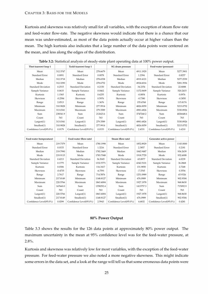
Table 3.2 shows the results of the analysis for 763 data points at approximately 100% power output.
The maximum uncertainty in the confidence level (95%) was noted for the steam flow-rate, at
0.25% of the mean. We also noted the large range for the steam flow-rate, which means that the
data is populated with one or more extreme outliers.
The interval at 95% confidence level was similar or lower for all the other variables.
24
Page 38
CHAPTER 3: BASIS FOR THE MODELS
Kurtosis and skewness was relatively small for all variables, with the exception of steam flow-rate
and feed-water flow-rate. The negative skewness would indicate that there is a chance that our
mean was under-estimated, as most of the data points actually occur at higher values than the
mean. The high kurtosis also indicates that a large number of the data points were centered on
the mean, and less along the edges of the distribution.
Table 3.2: Statistical analysis of steady-state plant operating data at 100% power output.Thot (narrow) loop 1 Tcold (narrow) loop 1 SG drum pressure Feed-water (pressure)
Mean 312.3747 Mean 278.6679 Mean 4911.1929 Mean 5277.3901
Standard Error 0.0091 Standard Error 0.0078 Standard Error 1.2394 Standard Error 0.8257
Median 312.3718 Median 278.6538 Median 4919.4121 Median 5277.2539
Mode 312.3290 Mode 278.6752 Mode 4924.6016 Mode 5281.3936
Standard Deviation 0.2515 Standard Deviation 0.2150 Standard Deviation 34.2354 Standard Deviation 22.8088
Sample Variance 0.0633 Sample Variance 0.0462 Sample Variance 1172.0609 Sample Variance 520.2415
Kurtosis 1.1565 Kurtosis 0.6255 Kurtosis -0.0854 Kurtosis 0.0976
Skewness -0.2584 Skewness 0.5976 Skewness -0.7380 Skewness -0.3850
Range 2.0513 Range 1.3676 Range 155.6768 Range 115.8174
Minimum 310.9828 Minimum 277.9914 Minimum 4826.0059 Minimum 5215.0752
Maximum 313.0341 Maximum 279.3589 Maximum 4981.6826 Maximum 5330.8926
Sum 238341.9 Sum 212623.6 Sum 3747240.2 Sum 4026648.6
Count 763 Count 763 Count 763 Count 763
Largest(1) 313.0341 Largest(1) 279.3589 Largest(1) 4981.6826 Largest(1) 5330.8926
Smallest(1) 310.9828 Smallest(1) 277.9914 Smallest(1) 4826.0059 Smallest(1) 5215.0752
Confidence Level(95.0%) 0.0179 Confidence Level(95.0%) 0.0153 Confidence Level(95.0%) 2.4331 Confidence Level(95.0%) 1.6210
Feed-water (temperature) Feed-water (flow-rate) Steam (flow-rate) Generator active power
Mean 219.7379 Mean 1780.1998 Mean 1852.8929 Mean 1143.0000
Standard Error 0.0153 Standard Error 1.3216 Standard Error 2.3857 Standard Error 0.2181
Median 219.7990 Median 1782.3469 Median 1842.9487 Median 936.2639
Mode 219.9115 Mode 1783.7048 Mode 1918.7729 Mode 932.6008
Standard Deviation 0.4213 Standard Deviation 36.5045 Standard Deviation 65.8977 Standard Deviation 6.0239
Sample Variance 0.1775 Sample Variance 1332.5771 Sample Variance 4342.5101 Sample Variance 36.2868
Kurtosis 0.0306 Kurtosis 116.3417 Kurtosis 131.9850 Kurtosis 2.7248
Skewness -0.4735 Skewness -6.7591 Skewness -7.3765 Skewness 0.3554
Range 2.7617 Range 714.5876 Range 1251.0989 Range 65.9326
Minimum 217.8149 Minimum 1148.8127 Minimum 676.0989 Minimum 902.9304
Maximum 220.5766 Maximum 1863.4004 Maximum 1927.1978 Maximum 968.8630
Sum 167660.0 Sum 1358292.4 Sum 1413757.3 Sum 715092.9
Count 763 Count 763 Count 763 Count 763
Largest(1) 220.5766 Largest(1) 1863.4004 Largest(1) 1927.1978 Largest(1) 968.8630
Smallest(1) 217.8149 Smallest(1) 1148.8127 Smallest(1) 676.0989 Smallest(1) 902.9304
Confidence Level(95.0%) 0.0299 Confidence Level(95.0%) 2.5943 Confidence Level(95.0%) 4.6832 Confidence Level(95.0%) 0.4281
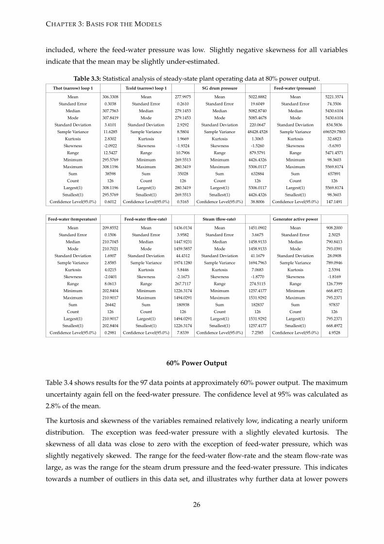
80% Power Output
Table 3.3 shows the results for the 126 data points at approximately 80% power output. The
maximum uncertainty in the mean at 95% confidence level was for the feed-water pressure, at
2.8%.
Kurtosis and skewness was relatively low for most variables, with the exception of the feed-water
pressure. For feed-water pressure we also noted a more negative skewness. This might indicate
some errors in the data set, and a look at the range will tell us that some erroneous data points were
25
Page 39
CHAPTER 3: BASIS FOR THE MODELS
included, where the feed-water pressure was low. Slightly negative skewness for all variables
indicate that the mean may be slightly under-estimated.
Table 3.3: Statistical analysis of steady-state plant operating data at 80% power output.Thot (narrow) loop 1 Tcold (narrow) loop 1 SG drum pressure Feed-water (pressure)
Mean 306.3308 Mean 277.9975 Mean 5022.8882 Mean 5221.3574
Standard Error 0.3038 Standard Error 0.2610 Standard Error 19.6049 Standard Error 74.3506
Median 307.7563 Median 279.1453 Median 5082.8740 Median 5430.6104
Mode 307.8419 Mode 279.1453 Mode 5085.4678 Mode 5430.6104
Standard Deviation 3.4101 Standard Deviation 2.9292 Standard Deviation 220.0647 Standard Deviation 834.5836
Sample Variance 11.6285 Sample Variance 8.5804 Sample Variance 48428.4528 Sample Variance 696529.7883
Kurtosis 2.8302 Kurtosis 1.9669 Kurtosis 1.3065 Kurtosis 32.6823
Skewness -2.0922 Skewness -1.9324 Skewness -1.5260 Skewness -5.6393
Range 12.5427 Range 10.7906 Range 879.5791 Range 5471.4571
Minimum 295.5769 Minimum 269.5513 Minimum 4426.4326 Minimum 98.3603
Maximum 308.1196 Maximum 280.3419 Maximum 5306.0117 Maximum 5569.8174
Sum 38598 Sum 35028 Sum 632884 Sum 657891
Count 126 Count 126 Count 126 Count 126
Largest(1) 308.1196 Largest(1) 280.3419 Largest(1) 5306.0117 Largest(1) 5569.8174
Smallest(1) 295.5769 Smallest(1) 269.5513 Smallest(1) 4426.4326 Smallest(1) 98.3603
Confidence Level(95.0%) 0.6012 Confidence Level(95.0%) 0.5165 Confidence Level(95.0%) 38.8006 Confidence Level(95.0%) 147.1491
Feed-water (temperature) Feed-water (flow-rate) Steam (flow-rate) Generator active power
Mean 209.8552 Mean 1436.0134 Mean 1451.0902 Mean 908.2000
Standard Error 0.1506 Standard Error 3.9582 Standard Error 3.6675 Standard Error 2.5025
Median 210.7045 Median 1447.9231 Median 1458.9133 Median 790.8413
Mode 210.7021 Mode 1459.5857 Mode 1458.9133 Mode 793.0391
Standard Deviation 1.6907 Standard Deviation 44.4312 Standard Deviation 41.1679 Standard Deviation 28.0908
Sample Variance 2.8585 Sample Variance 1974.1280 Sample Variance 1694.7963 Sample Variance 789.0946
Kurtosis 4.0215 Kurtosis 5.8446 Kurtosis 7.0683 Kurtosis 2.5394
Skewness -2.0401 Skewness -2.1673 Skewness -1.8770 Skewness -1.8169
Range 8.0613 Range 267.7117 Range 274.5115 Range 126.7399
Minimum 202.8404 Minimum 1226.3174 Minimum 1257.4177 Minimum 668.4972
Maximum 210.9017 Maximum 1494.0291 Maximum 1531.9292 Maximum 795.2371
Sum 26442 Sum 180938 Sum 182837 Sum 97837
Count 126 Count 126 Count 126 Count 126
Largest(1) 210.9017 Largest(1) 1494.0291 Largest(1) 1531.9292 Largest(1) 795.2371
Smallest(1) 202.8404 Smallest(1) 1226.3174 Smallest(1) 1257.4177 Smallest(1) 668.4972
Confidence Level(95.0%) 0.2981 Confidence Level(95.0%) 7.8339 Confidence Level(95.0%) 7.2585 Confidence Level(95.0%) 4.9528
60% Power Output
Table 3.4 shows results for the 97 data points at approximately 60% power output. The maximum
uncertainty again fell on the feed-water pressure. The confidence level at 95% was calculated as
2.8% of the mean.
The kurtosis and skewness of the variables remained relatively low, indicating a nearly uniform
distribution. The exception was feed-water pressure with a slightly elevated kurtosis. The
skewness of all data was close to zero with the exception of feed-water pressure, which was
slightly negatively skewed. The range for the feed-water flow-rate and the steam flow-rate was
large, as was the range for the steam drum pressure and the feed-water pressure. This indicates
towards a number of outliers in this data set, and illustrates why further data at lower powers
26
Page 40
CHAPTER 3: BASIS FOR THE MODELS
were not included.
Table 3.4: Statistical analysis of steady-state plant operating data at 60% power output.Thot (narrow) loop 1 Tcold (narrow) loop 1 SG drum pressure Feedwater (pressure)
Mean 294.4966 Mean 272.9632 Mean 4889.1592 Mean 5054.5517
Standard Error 0.5062 Standard Error 0.5418 Standard Error 49.6826 Standard Error 71.0407
Median 292.4999 Median 270.2350 Median 4636.5977 Median 4873.4805
Mode 290.8120 Mode 270.9615 Mode 4558.7588 Mode 4879.1221
Standard Deviation 4.9851 Standard Deviation 5.3356 Standard Deviation 489.3164 Standard Deviation 699.6701
Sample Variance 24.8517 Sample Variance 28.4689 Sample Variance 239430.5181 Sample Variance 489538.2821
Kurtosis -0.8792 Kurtosis -1.0424 Kurtosis -0.7333 Kurtosis 27.6735
Skewness 0.6545 Skewness 0.8911 Skewness 1.0138 Skewness -3.6057
Range 18.1624 Range 15.4915 Range 1442.6123 Range 6012.1163
Minimum 286.6025 Minimum 266.8803 Minimum 4405.6758 Minimum 0.0947
Maximum 304.7649 Maximum 282.3718 Maximum 5848.2881 Maximum 6012.2109
Sum 28566.2 Sum 26477.4 Sum 474248.4 Sum 490291.5
Count 97 Count 97 Count 97 Count 97
Largest(1) 304.7649 Largest(1) 282.3718 Largest(1) 5848.2881 Largest(1) 6012.2109
Smallest(1) 286.6025 Smallest(1) 266.8803 Smallest(1) 4405.6758 Smallest(1) 0.0947
Confidence Level(95.0%) 1.0047 Confidence Level(95.0%) 1.0754 Confidence Level(95.0%) 98.6191 Confidence Level(95.0%) 141.0147
Feed-water (temperature) Feed-water (flow-rate) Steam (flow-rate) Generator active power
Mean 194.7248 Mean 1023.4041 Mean 1083.4404 Mean 670.1000
Standard Error 0.5771 Standard Error 14.1036 Standard Error 14.6660 Standard Error 5.9112
Median 195.6016 Median 1023.9580 Median 1069.9634 Median 562.6365
Mode #N/A Mode 1102.9160 Mode 1126.1294 Mode 427.4718
Standard Deviation 5.6838 Standard Deviation 138.9048 Standard Deviation 144.4435 Standard Deviation 58.2184
Sample Variance 32.3056 Sample Variance 19294.5463 Sample Variance 20863.9244 Sample Variance 3389.3867
Kurtosis 0.6149 Kurtosis 2.3748 Kurtosis 3.2206 Kurtosis -1.1387
Skewness 0.4119 Skewness 0.9159 Skewness 1.1238 Skewness -0.2896
Range 26.2863 Range 740.6776 Range 795.4517 Range 213.1866
Minimum 185.3304 Minimum 776.4083 Minimum 805.9829 Minimum 426.7391
Maximum 211.6167 Maximum 1517.0859 Maximum 1601.4346 Maximum 639.9258
Sum 18888.3 Sum 99270.2 Sum 105093.7 Sum 53393.7
Count 97 Count 97 Count 97 Count 97
Largest(1) 211.6167 Largest(1) 1517.0859 Largest(1) 1601.4346 Largest(1) 639.9258
Smallest(1) 185.3304 Smallest(1) 776.4083 Smallest(1) 805.9829 Smallest(1) 426.7391
Confidence Level(95.0%) 1.1455 Confidence Level(95.0%) 27.9955 Confidence Level(95.0%) 29.1118 Confidence Level(95.0%) 11.7336
The mean for each plant parameter thus collectively form a set of plant data values.
At 60% power output, in Table 3.4, it can be seen that the largest interval for the 95% confidence
level is for the feed-water pressure at 2.7% . The uncertainty gets larger as there were less data
points, but still meaningful analysis could be done at both 80% and 60% power outputs.
3.2 Preliminary steady-state calculations
A preliminary calculation was performed using EES (Engineering Equation Solver) to determine
the relevant primary side conditions for the model. This was done as the primary side data was
not directly available in the form required for inputs to the simulation model. The steady-state
also serve as a verification of the input and output parameters of the model. More in-depth
mathematical verification of both software packages has been performed in previous studies
(RELAP5, 2001d; van der Merwe et al., 2006).
27
Page 41
CHAPTER 3: BASIS FOR THE MODELS
The mass flow-rate of the primary side was not directly accessible from the data provided by
Koeberg. It was, therefore, necessary to first calculate the primary side conditions of the steam
generator before running simulations.
This was done by assuming the steady-state operation of the SG. With the secondary conditions
known, it was possible to calculate the total heat transferred from the inlet and outlet enthalpies.
As the SG is assumed to be at steady-state, the heat transferred to the secondary side is equal to
the heat transferred from the primary side. With this information, we could calculate the primary
mass flow with Equation 3.2.1.
Q = ms · (hso − hsi) = mp · (hpo − hpi) (3.2.1)
In order to directly calculate the primary mass flow-rate, however, it is necessary to know the
inlet and outlet enthalpies of the primary side. This was calculated from the temperature and
pressure conditions at the inlet and the outlet. The inlet conditions were obtained from the Safety
Analysis Report from Koeberg (ESKOM, 2004). The primary outlet conditions were calculated
from a pressure drop calculation described below.
Pressure drop
The Reynolds number is a common dimensionless number used in fluid analysis, and was
calculated here for the primary fluid in the tubes. It gives us an indication of whether the flow is
in the laminar or turbulent regime. We expect all flow in the steam generator to be turbulent,
with a high Reynolds number.
Rep =ρp · vp · Dh,p
µp(3.2.2)
The velocity in the primary circuit was calculated from the density and the average flow area. The
mass flow-rate is used here when calculated from Equation 3.2.1.
vp =mp
ρp · Ap(3.2.3)
The friction factor was then calculated using the Haaland correlation (Thome, 2004). The
roughness of stainless steel was used here, approximately ε = 30µm (Flownex, 2011a).
f = (1
−1.8 · log10[(ε/Dh,p
3.7 )1.11 + 6.9Rep
)2 (3.2.4)
28
Page 42
CHAPTER 3: BASIS FOR THE MODELS
The head-loss associated with the friction factor was then calculated for the lengths of the tubes.
hl = f · (Lp
Dh,p) · (
v2p
2 · g ) (3.2.5)
The pressure drop across the primary side was calculated from the head loss.
∆Pp = ρp · g · hl (3.2.6)
Implicit mass flow-rate
In Equation 3.2.1 we can see that the primary side mass flow-rate can only be calculated if the
primary inlet and outlet conditions are known. The outlet conditions, however, are a function of
the pressure drop, which in turn is a function of the mass flow-rate. This can be seen in Equations
3.2.2 through 3.2.6. The friction factor, and thus also the pressure drop, is a function of the
Reynolds number which in turn is a function of the flow velocity or mass flow-rate.
The primary outlet conditions are, therefore, initially guessed. New outlet conditions are
calculated from the resulting pressure drop, and the calculation is iterated until guessed
conditions converge with the calculated conditions.
3.3 Simplification of the geometry
Figure 3.1 shows the general geometry of the original steam generators installed at Koeberg NPP.
It specifies the upper internals, including the geometry for the dryers and separators. It also
specifies the geometry for the primary tubes. Some important geometrical aspects are the number
and diameter of the separator and dryer stages. The flow paths for these components should be
modelled separately (RELAP5, 2001c). The details for the tube bundle are also important. The heat
transfer surface area of 4 699m2 is used for a total of 3 330 tubes. The inner and outer diameters
were given, as well as the square pitch. Also from the drawing, we are able to get the length of the
SG, the spherical radius of the inlet plenums and the outside diameters of the lower and upper SG
shell.
The final dimensions are shown in Figures 3.2 to 3.7.
The geometry for the flow areas was simplified to suit the scope of the project. The geometry from
the technical documents were condensed to a set of one dimensional geometries suitable for the
application of the one-dimensional model.
The simplified cross-section of the primary inlet plenum is shown in Figure 3.2. It was modelled
as a cylinder, of the same radius as the spherical radius specified in the documents.
The boiler region consists of the primary tubes and the channels between the tubes for secondary
flow. Dimensions for the down-comer were also included. A schematic is shown in Figure 3.3.
29
Page 43
CHAPTER 3: BASIS FOR THE MODELS
Figure 3.1: General geometry of the Koeberg SG (ESKOM)
30
Page 44
CHAPTER 3: BASIS FOR THE MODELS
R 1595mm
Figure 3.2: Inlet plenum geometry used for the model)
64mm
32.54mm
22.22mm
1.27mm
3455mm
Figure 3.3: Geometry of the boiler region
31
Page 45
CHAPTER 3: BASIS FOR THE MODELS
The geometry of the riser consists mostly of the down-comer region that allows for recirculating
flow. It is shown in Figure 3.4.
4480mm
74mm
Figure 3.4: Geometry of the riser region
1422mm
4480mm
Figure 3.5: Geometry of the separator region
The geometry for the separators and the dryer stages is shown in Figure 3.5 and 3.6. The flow
areas for the separator stage consist of the three centrifugal separator cylinders. The cylinders are
shown in the figures as 3 circles, as they move vertically up through the upper shell of the SG.
The dryer stage is shown for clarity, but they were not modelled as custom flow resistances were
added to the separator components to increase stability of the solution (RELAP5, 2001c). The
dashed lines indicate where the dryer’s would be situated in an actual model, but they do not
significantly obstruct the flow so they were omitted to simplify the separation calculation.
The geometry of the steam dome was modelled as a simple cylindrical pipe. The outlet was linked
to a time dependent volume, or boundary conditions simulating the turbine.
32
Page 46
CHAPTER 3: BASIS FOR THE MODELS
4480mm
Figure 3.6: Geometry of the dryer region
4480mm
Figure 3.7: Geometry of the steam dome region
33
Page 47
CHAPTER 3: BASIS FOR THE MODELS
3.4 Geometry and Heat Structure inputs
The volumetric inputs for the model are shown in Table 3.5. These are the flow areas, volume
lengths, hydraulic diameter, circumference and flow volume used for each of the components of
the model.
Table 3.5: Volumetric inputs for the steam generator modelPrimary Side Components
Component Flownex RELAP5 No. of vol. L (m) D_h (m) Circum. (m) FA (m2) V (m3) Inc. (◦)
Primary Inlet Volume P-101 tmpdvol 101 1 - 0.518 - 90
Primary Inlet Header/Plenum P-103 snglvol 103 1 1.063 3.996 4.249 90
U-Tube-1 P-110-1
pipe 110 10 11.412 0.01968 1.013 11.560
90
U-Tube-2 P-110-2 90
U-Tube-3 P-110-3 90
U-Tube-4 P-110-4 90
U-Tube-5 P-110-5 90
U-Tube-6 P-110-6 -90
U-Tube-7 P-110-7 -90
U-Tube-8 P-110-8 -90
U-Tube-9 P-110-9 -90
U-Tube-10 P-110-10 -90
Primary Outlet Header/Plenum P-106 snglvol 106 1 1.063 3.996 4.249 -90
Primary Outlet Volume P-108 tmdpvol 108 1 - 0.7850 - -90
Secondary Side Components
Component Flownex RELAP5 No. of vol. L (m) D_h (m) Circum. (m) FA (m2) V (m3) Inc. (◦)
Feed-water Inlet Volume S-201 tmdpvol 201 1 - - - 0
Feed-water Inlet Pipe S-203 snglvol 203 1 3.000 0.518 1.554 0
Feed-water Branch S-225 branch 225 1 -90
Down-comer Annulus S-214 annulus 214 5 11.412 0.682 7.781 -90
Heated Riser Region 1 S-215-1
pipe 215 5 11.412 0.0385 815.956 7.402 84.473 90
Heated Riser Region 2 S-215-2
Heated Riser Region 3 S-215-3
Heated Riser Region 4 S-215-4
Heated Riser Region 5 S-215-5
Unheated Riser Region S-216 snglvol 216 1 0.833 14.739 12.280 90
Separator Riser S-221 snglvol 221 1 2.058 4.764 9.803 90
Dryers Riser S-222 separatr 222 1 2.058 15.763 32.433 90
Reflux Down-comers S-224 annulus 224 1 2.058 10.999 22.630 -90
Steam Dome S-250 separatr 250 1 1.627 15.763 25.647 90
Steam Outlet Volume S-260 tmdpvol 260 1 - - - 90
The heat structure inputs for both RELAP5 and Flownex are shown in Table 3.6. The geometry of
the heat structure was taken from the primary tube geometry. The heat structure models the tube
material, and in both RELAP5 and Flownex, the material was chosen to be stainless steel.
34
Page 48
CHAPTER 3: BASIS FOR THE MODELS
Table 3.6: Heat structure inputs for the steam generator model
Heat Structures
Component From To Left SA (m2) Right SA (m2) Length (m) Mesh Points dx (m) Thickness (m)
Tubing P-110 S-215 4699 5305 22.8 5 0.0003175 0.00127
3.5 Model Development
The codes and inputs developed for the model are given in Appendix E and D for Flownex and
RELAP5 respectively. The geometry and nodalization for both models were the same, as discussed
in the previous section. The following subsections discuss the subtle differences in the setups.
3.5.1 RELAP5 - Two-Fluid
The nodalization used for RELAP5 is shown in Figure 3.8. The boundary conditions were
represented by time-dependent volumes.
Due to the complicated nature of the SG internals, it was necessary to add custom flow losses to
some of the junctions in order to simulate the correct re-circulation ratio (RELAP5, 2001c). The
flow losses were adjusted in junction 206 (the junction entering the boiler region) so that a re-
circulation ratio of 3.8 was achieved at 100% power output. The value of 3.8 was taken from
Desfontaines-Leromain (2004), and is a standard design reference. The actual recirculation within
the steam generator may vary from design due to a tube plugging, leakage or many of the other
issues discussed in the previous chapter.
Further flow losses were added to the separator junctions to increase stability of the solution,
in accordance with RELAP5 (2001c). When flow-losses were added to the separator, they were
subtracted from the flow losses added to junction 206. This was done to maintain the re-circulation
ratio, while still maintaining stability of the outlet quality.
The flow losses added to the separator were justified because RELAP5 models the separator
components as a black box. The void fraction of the outlet steam and the return liquid is a
function of the calculated void fraction within the steam separator component at any given time
step. More detailed models of the steam separator components were available, but data to
support the models were not.
The steam generator inputs were then left unchanged when run at 80% and 60% conditions.
Boundary conditions
The boundary conditions specified to RELAP5 for 100%, 80% and 60% power output conditions
are shown in Table 3.7, Table 3.8 and Table 3.9.
35
Page 49
CHAPTER 3: BASIS FOR THE MODELS
Figure 3.8: Nodalization of the steam generator model for RELAP5
36
Page 50
CHAPTER 3: BASIS FOR THE MODELS
The primary mass flow-rate and the primary outlet pressure were calculated in Section 3.2 of this
report. The inlet mass flow-rate and inlet temperature were then specified to the primary and
secondary circuit. The pressure and quality were specified for the outlet volumes of the primary
and the secondary circuit.
The inlet pressure specified for the time-dependent volume is irrelevant to the calculation, as
the time-dependent junction forces the mass-flow to the specified value (RELAP5, 2001c). The
pressure of the time-dependent volume was therefore not used in the pressure calculation of the
rest of the system.
Table 3.7: Boundary conditions specified to RELAP5 for 100% power output.
m_dot (kg/s) T (◦C) or Quality P (MPa)
Primary Inlet BC 6316 312
Primary Outlet BC 0.0 14.825
Secondary Inlet BC 618 219
Secondary Outlet BC 1.0 4.911
Table 3.8: Boundary conditions specified to RELAP5 at 80% power output.
m_dot (kg/s) T (◦C) or Quality P (MPa)
Primary Inlet BC 6051 306
Primary Outlet BC 0.0 14.886
Secondary Inlet BC 479 220
Secondary Outlet BC 1.0 5.023
Table 3.9: Boundary conditions specified to RELAP5 for 60% power output.
m_dot (kg/s) T (◦C) or Quality P (MPa)
Primary Inlet BC 6057 294
Primary Outlet BC 0.0 14.897
Secondary Inlet BC 341 195
Secondary Outlet BC 1.0 4.889
3.5.2 RELAP5 - Homogeneous
The development of the homogeneous RELAP5 model followed the same procedure as with the
two-fluid model. The nodalization from Figure 3.8 was used. The difference lies in the fact that the
homogeneous model was chosen for the solution of all the components except for the separator.
37
Page 51
CHAPTER 3: BASIS FOR THE MODELS
The two-fluid model is needed for the separator volume so that steam and liquid separation may
take place in the component. The remainder of the model, including the boiler region, used the
homogeneous solution. In RELAP5, this was achieved by setting the homogeneous switch on for
each component except for the separator.
The custom flow losses were again added to junction 206 so that the re-circulation ratio was
approximately 3.8.
Additional flow losses were added to the separator junctions to increase stability of the solution.
To monitor stability, the outlet steam quality was monitored. It was found to oscillate wildly when
unstable, and settle to a steady-state when brought to stability.
3.5.3 Flownex
The nodalization of the model used in Flownex is shown in Figure 3.9. The volumes mostly
consist of pipe volumes and heat structure components. The separator was modelled with a two-
phase tank. The separator component (or two-phase tank) behaves ideally, removing all steam
and returning all liquid in the entering stream. The inputs set for the model may be found on the
CD-ROM attached with this report.
Figure 3.9: Nodalization of the steam generator model for Flownex
38
Page 52
CHAPTER 3: BASIS FOR THE MODELS
Heat transfer correlation script
The heat transfer correlation was custom written, as Flownex only provides a built in correlation
for single-phase heat transfer using the Dittus-Boelter correlation. The boiling phenomenon is
complicated, and the heat transfer more so. There are many flow and boiling regimes applicable
over the steam generator (Green and Hetsroni, 1995), and it is thus difficult to model accurately.
It was simplified by assuming that the Chen correlation can describe the heat transfer through the
entire range of the boiler.
Flownex provides functionality to include EES scripts in the model. The flow parameters were
calculated and sent to the EES script (see Appendix B) where two-phase parameters were
calculated that weren’t available in Flownex. The EES script then sent the parameters to the
custom C# script included in Flownex. The Chen correlation was implemented with a C# script,
utilizing the parameters received from the EES script. The C# script then calculated the heat
transfer coefficient, and sent it to the heat transfer component.
The process is therefore iterative, and the steady-state was calculated until the heat transfer
coefficient converged. The code for the Chen correlation script may be found in Appendix C. The
EES script for calculating the two-phase parameters may be found in Appendix B.
Boundary conditions
The boundary conditions specified to the model in Flownex for 100%, 80% and 60% power
conditions are shown in Table 3.10, Table 3.11 and Table 3.12 respectively.
The mass flow-rate and temperature were specified for the inlets of both the primary and
secondary circuits. The outlet pressure was specified for the primary and secondary circuits.
Table 3.10: Boundary conditions specified to Flownex for 100% power output.
m_dot (kg/s) T (◦C) P (MPa)
Primary Inlet BC 6316 312
Primary Outlet BC 14.825
Secondary Inlet BC 618 219
Secondary Outlet BC 4.911
39
Page 53
CHAPTER 3: BASIS FOR THE MODELS
Table 3.11: Boundary conditions specified to Flownex for 80% power output.
m_dot (kg/s) T (◦C) P (MPa)
Primary Inlet BC 6051 306
Primary Outlet BC 14.886
Secondary Inlet BC 479 220
Secondary Outlet BC 5.023
Table 3.12: Boundary conditions specified to Flownex at 60% power output.
m_dot (kg/s) T (◦C) P (MPa)
Primary Inlet BC 6057 294
Primary Outlet BC 14.897
Secondary Inlet BC 341 195
Secondary Outlet BC 4.889
40
Page 54
CHAPTER 4
Results and discussion
4.1 Comparison with empirical data
The models were validated against the plant operating data obtained from Koeberg NPP, as was
discussed in Section 3.1 of this report. The arithmetic mean from the plant parameters were used
as a single value describing each condition of 100%, 80% and 60% power output. In Table 4.1,
Table 4.2 and Table 4.3 the results from the RELAP5 and Flownex models are tabulated against
these values. The error is reported for each variable for each model.
4.1.1 100% Power Output
Table 4.1 shows the Koeberg data describing the 100% power level tabulated against the results
from RELAP5 and Flownex.
Table 4.1: Steady-state validation of the model at 100% power outputT_pi (◦C) T_po (◦C) P_so (kPa) P_si (kPa) T_si (◦C) x_so m_dot_s (kg/s) Q_boiler (MW) R_circ
100% Power
Koeberg 312 279 4911 5277 220 1.000 618 1143 3.80
RELAP5 - Two-Fluid 312 279 4912 4942 220 1.000 610 1131 3.81
Error % -0.1 0.0 0.0 -6.4 0.1 0.0 -1.3 -1.0 0.2
RELAP5 - Homogeneous 312 279 4911 4924 220 1.000 604 1121 3.81
Error % -0.1 0.1 0.0 -6.7 0.1 0.0 -2.2 -1.9 0.3
Flownex - Homogeneous 312 280 4911 4951 220 1.000 618 1092 3.80
Error % -0.1 0.4 0.0 -6.2 0.1 0.0 0.1 -4.4 -0.1
The largest errors were -6.4%, -6.7% and -6.2% for the secondary inlet pressure calculated by the
RELAP5 two-fluid, homogeneous and Flownex models respectively.
The errors for the heat transferred in the boiler for the RELAP5 two-fluid, homogeneous and
Flownex models were -1.0%, -1.9% and -4.4% respectively. The slight underestimation by RELAP5
was attributed to the fact that the heat transfer correlations slightly under-estimate the actual
heat-transfer which occurs (RELAP5, 2001b). In Flownex, where we exclusively used the Chen
correlation, we saw an even larger under-estimation in heat transfer.
41
Page 55
CHAPTER 4: RESULTS AND DISCUSSION
The flow-rate of steam was under-estimated by 1.3% and 2.2% by the RELAP5 two-fluid and
homogeneous models, respectively. The mass flow-rate reported in the results corresponds to the
outlet steam flow-rate. While the feed-water flow-rate is kept constant, as described in Chapter
3, there are instabilities brought in by the steam separator component (RELAP5, 2001c). These
instabilities result in oscillations of the steam flow-rate exiting the separator. By adding flow
losses to the separator component, as described in the previous section, these oscillations may be
reduced (RELAP5, 2001c).
4.1.2 80% Power Output
The models were developed specifically to achieve a re-circulation ratio of 3.8 at 100% power
output. This was done by adjusting flow losses through the boiler region as well as the separator
component. The subsequent calculations at lower power levels such as 80% and 60% were done
without adjusting flow losses further. In this way, we were able to see how the model reacts to
various power levels.
Table 4.2 shows the Koeberg data values tabulated against the values calculated by RELAP5 and
Flownex.
Table 4.2: Steady-state validation of the model at 80% power outputT_pi (◦C) T_po (◦C) P_so (kPa) P_si (kPa) T_si (◦C) x_so m_dot_s (kg/s) Q_boiler (MW) R_circ
80% Power
Koeberg 306 278 5023 5221 210 1.000 479 908 5.00
RELAP5 - Two-Fluid 306 277 5026 5057 210 1.000 483 916 4.89
Error % -0.1 -0.2 0.1 -3.1 0.1 0.0 0.9 0.9 -2.1
RELAP5 - Homogeneous 306 277 5023 5051 210 1.000 485 919 5.81
Error % -0.1 -0.3 0.0 -3.3 0.1 0.0 1.4 1.2 16.2
Flownex - Homogeneous 306 278 5023 5049 210 1.000 479 892 4.84
Error % -0.1 0.0 0.0 -3.3 0.1 0.0 0.1 -1.8 -3.1
The largest errors were again the inlet pressure calculated for the secondary circuit. The RELAP5
two-fluid model calculates an error of -3.1%, while the RELAP5 homogeneous model and Flownex
both calculated an error of -3.3%.
The error in heat transfer calculated by the RELAP5 two-fluid model, the RELAP5 homogeneous
model and Flownex were 0.9%, 1.2% and -1.8% respectively.
The error in the steam flow-rate was 0.9% and 1.4% for the RELAP5 two-fluid and homogeneous
models, respectively.
4.1.3 60% Power Output
Table 4.3 shows the Koeberg data tabulated against the results calculated from RELAP5 and
Flownex.
42
Page 56
CHAPTER 4: RESULTS AND DISCUSSION
Table 4.3: Steady-state validation of the model at 60% power outputT_pi (◦C) T_po (◦C) P_so (kPa) P_si (kPa) T_si (◦C) x_so m_dot_s (kg/s) Q_boiler (MW) R_circ
60% Power
Koeberg 294 273 4889 5055 195 1.000 341 670 7.00
RELAP5 - Two-Fluid 294 273 4892 4892 195 0.982 341 660 6.37
Error % -0.2 -0.1 0.1 -3.2 0.1 -1.8 0.0 -1.5 -9.1
RELAP5 - Homogeneous 294 273 4889 4916 195 0.987 341 663 7.66
Error % -0.2 -0.1 0.0 -2.7 0.1 -1.3 0.0 -1.0 9.4
Flownex - Homogeneous 294 273 4889 4919 195 1.000 341 666 6.63
Error % -0.2 -0.2 0.0 -2.7 0.1 0.0 0.0 -0.6 -5.2
The error in the pressure calculation was -3.2%, -2.7% and -2.7% for the RELAP5 two-fluid,
homogeneous and Flownex models respectively.
The error in heat transfer was -1.5%, -1.0% and -0.6% for the RELAP5 two-fluid, homogeneous
and Flownex models respectively.
The quality of the exit steam was calculated to have a larger error at lower power levels. The
RELAP5 two-fluid and homogeneous solution calculated an error of -1.8% and -1.3% respectively.
4.2 Detailed inter-model comparisons
The results from RELAP5 showed that the flow regime through the first 3 vertical volumes of
the boiling region (corresponding to the first 6.85m in height) was in the sub-cooled nucleate
boiling regime, in which the Chen correlation and the Bergles-Rohsenow correlation is used to
calculate the heat transfer. The upper height of the shell side (the remaining 4.56m) was in the
saturated nucleate boiling regime, applying the Chen correlation as well as the Araki correlation
to the solution (discussed in Section 2.2.1). The reason the Chen correlation is not used exclusively
is because the correlation used within RELAP5 also varies with the surface and geometry type
specified. The results show, however, that the assumption of the boiling regime is correct, and
that the Chen correlation does indeed apply in the boiler region.
This was true at 100%, 80% and 60% power, and shows that the initial assumption that the Chen
correlation will dominate heat transfer effect was accurate.
It was not possible to analyze the micro- and macro-scopic parts of the Chen correlation from
RELAP5, and due to this inability, was omitted from the results in Flownex as well.
4.2.1 Primary side temperatures
The primary side temperatures calculated for the models at 100%, 80% and 60% power output
are shown in Figure 4.1, Figure 4.2 and Figure 4.3 respectively. The middle of the graph at 11m
represents the top of the tube bundle. The left half of the graph below 11m represents the upwards
portion of the tube bundle, while the right side represents the downward section.
43
Page 57
CHAPTER 4: RESULTS AND DISCUSSION
Figure 4.1: Primary side fluid temperatures at 100% power output
Figure 4.2: Primary side fluid temperatures at 80% power output
There was no noticeable difference between the RELAP5 two-fluid and homogeneous solution
at any power level. The Flownex solution approached the RELAP5 solution at higher qualities,
indicating that the heat transfer correlation in Flownex might be the cause of the error, and not the
homogeneous assumption.
The Flownex solution differed by as much as 5◦C from the RELAP5 solution in the first half of the
44
Page 58
CHAPTER 4: RESULTS AND DISCUSSION
Figure 4.3: Primary side fluid temperatures at 60% power output
tubes. The difference decreased with decreasing power levels. The difference was attributed to
the use of the Chen correlation in Flownex over the entire range of the boiler.
4.2.2 Quality through the boiler
The quality of the secondary fluid flowing through the boiler region was calculated and is shown
in Figure 4.4, Figure 4.5 and Figure 4.6 respectively.
At 100% power output there was little difference between the homogeneous and two-fluid
solutions from RELAP5. At lower powers, there was a marked difference between the two
solutions. At 80% and 60% power output, the quality calculated by the homogeneous model was
up to 4% less than calculated by the two-fluid model. The difference between the quality
calculated by the two models increased linearly as the quality and elevation above the tube-sheet
increases.
The Flownex model predicted a lower quality than the RELAP5 model by up to 0.05 throughout
the range of the boiler region. At 100%, where the difference between the homogeneous solution
and the two-fluid solution was small, the error was largely attributed to the heat transfer
correlation used in Flownex. At 80% and 60% power levels, the RELAP5 homogeneous solution
approached the Flownex solution at higher qualities.
In the RELAP5 model, boiling starts at close to 0m above the tube-sheet, as there is already
significant quality increase in the first volume. In the Flownex model, boiling starts in the second
volume. This may be attributed to the inability of the homogeneous model to accurately calculate
45
Page 59
CHAPTER 4: RESULTS AND DISCUSSION
Figure 4.4: Secondary quality through the boiler region at 100% power output
Figure 4.5: Secondary quality through the boiler region at 80% power output
the water level in the two-phase solution. In reality, the flow at the bottom of the tube bundle is
chaotic and frothy, and no true water line exists. In the Flownex model, the bottom volume still
consists only of water, and so the heat transfer coefficient is reduced and boiling starts a short
while later than the RELAP5 model.
46
Page 60
CHAPTER 4: RESULTS AND DISCUSSION
Figure 4.6: Secondary quality through the boiler region at 60% power output
4.2.3 Heat transfer coefficient on the surface of the tubes
The heat transfer coefficient in Flownex was calculated by the custom C# script described in the
previous chapter. The heat transfer coefficient in RELAP5 was calculated by using the matrix of
correlations described in Chapter 2. The comparison of the results are shown in Figure 4.7, Figure
4.8 and Figure 4.9 for 100%, 80% and 60% power output respectively.
A large difference between the homogeneous solution and the two-fluid solution occurred at the
inlet and outlet ends of the tubes near the tube-sheet. A difference of approximately 11 000 Wm2·K
was calculated at both ends. There was little to no difference between the RELAP5 homogeneous
and the two-fluid model over the remainder of the tubes. The small difference was attributed to
the water-level in the boiler region existing within the first and lowest volume. The homogeneous
model cannot account for the water-level, and thus uses a single-phase heat transfer correlation in
the lower regions. At lower power levels there was little difference between the two models.
The heat transfer coefficient calculated by the custom Flownex script was lower than RELAP5 by
up to 12 000 Wm2·K across the range of the boiler. The discrepancy was expected in the lower regions
of the boiler. However, the large difference across the rest of the boiler would indicate that the
Chen correlation should not be used exclusively for boiling heat transfer.
The large difference in the calculated heat transfer coefficients was attributed to the fact that
Flownex uses the Chen correlation exclusively over the range of conditions through throughout
the boiler region. RELAP5 uses a matrix of correlations, as described in Chapter 2, which results
in a more accurate prediction than we get with our rudimentary script.
47
Page 61
CHAPTER 4: RESULTS AND DISCUSSION
Figure 4.7: Heat transfer coefficient on the surface of the tubes at 100% power output.
Figure 4.8: Heat transfer coefficient on the surface of the tubes at 80% power output.
4.2.4 Flow velocity through the boiler region
The flow velocity for the homogeneous, liquid and vapour fluids flowing through the boiler region
are shown in Figure 4.10, Figure 4.11 and Figure 4.12 respectively.
The homogeneous model approximated the two-fluid velocity well at low elevations and low
48
Page 62
CHAPTER 4: RESULTS AND DISCUSSION
Figure 4.9: Heat transfer coefficient on the surface of the tubes at 60% power output.
Figure 4.10: Flow velocity through the boiler region at 100% power output.
quality. Above 4m, and thus at higher quality, the homogeneous flow velocity appeared to
approximate the average between the fluid and vapour velocities. At 100%, the vapour velocity
at 11m was calculated by RELAP5 to be almost 6 m/s, while the homogeneous flow was
calculated as 3 m/s. At 60%, the difference was smaller at 1 m/s.
There was a small difference between flow velocities calculated by RELAP5 and Flownex. At
49
Page 63
CHAPTER 4: RESULTS AND DISCUSSION
Figure 4.11: Flow velocity through the boiler region at 80% power output.
Figure 4.12: Flow velocity through the boiler region at 60% power output.
100% and 1m, the difference was 0.6 m/s. The difference gets smaller as the elevation and quality
increases.
50
Page 64
CHAPTER 4: RESULTS AND DISCUSSION
4.2.5 Tube surface temperature on secondary side
The surface temperature on the secondary side of the tubes are shown in Figure 4.13, Figure 4.14
and Figure 4.15 respectively.
Figure 4.13: Secondary surface temperatures on the tubes 100% power output.
Figure 4.14: Secondary surface temperatures on the tubes 80% power output.
The difference between the homogeneous model and the two-fluid model was most apparent at
51
Page 65
CHAPTER 4: RESULTS AND DISCUSSION
Figure 4.15: Secondary surface temperatures on the tubes 60% power output.
the end points of the tubes. There was a difference of approximately 5◦C at the ends of the tubes at
100%, but no difference at lower power levels. The difference at low elevations was expected due
to the inaccuracy of the homogeneous model in modelling the water-level in the boiler region.
There was a large difference between the Flownex solution and the RELAP5 solution in at the
end points of the tubes. The temperature at 1m and 100% was larger in Flownex by almost 25◦C.
The difference decreases drastically along the tube length, and was therefore attributed to the
lower quality predicted by Flownex. Over the remainder of the tube surface, the Flownex solution
follows the trend of the heat transfer coefficient. The surface temperatures calculated by Flownex
were slightly larger by approximately 3◦C over the remainder of the tube surface.
4.2.6 Heat flux on the surface of the tubes
The heat flux calculated on the secondary surface of the tubes for the various models are shown
in Figure 4.16, Figure 4.17 and Figure 4.18 respectively.
There was a slight difference between the homogeneous and the two-fluid models at the end
points of the tubes. The heat flux predicted by the homogeneous model was lower by as much as
50 kWm2 at 1m and 100%. There was less difference between the models at lower power levels.
There was a large difference between the heat flux predicted by Flownex and RELAP5. As
expected, at the end points of the tubes we saw enlarged differences between the models. The
difference were as large as 170 kWm2 at 1m and 100%. At lower power levels, the difference was still
large, as high as 200 kWm2 at 4m and 80%. The Flownex solution approaches the RELAP5 solution
52
Page 66
CHAPTER 4: RESULTS AND DISCUSSION
Figure 4.16: Heat flux on the surface of the tubes at 100% power output.
Figure 4.17: Heat flux on the surface of the tubes at 80% power output.
at higher elevations above the tube sheet. The difference being slightly lower at a maximum of
120 kWm2 at 7m and 80%.
53
Page 67
CHAPTER 4: RESULTS AND DISCUSSION
Figure 4.18: Heat flux on the surface of the tubes at 60% power output.
4.3 Summary of inter-model comparison
The results were focussed on the boiler region, where the heat transfer from primary to secondary
side occurs.
The primary side temperatures calculated by Flownex deviate by a maximum of 5◦C from those
calculated by RELAP5. The largest deviations were observed closest to the tube-sheet, at the inlet
and outlet ends of the tube bundle. Deviations between the RELAP5 homogeneous fluid solution
and the RELAP5 two-fluid solution were negligible.
The secondary side quality calculated by Flownex deviated by a maximum of 5% when compared
with the quality calculated by RELAP5. The largest deviation occurred in the region closest to
the tube-sheet where the water-level affects the homogeneous solution. At 100% power there was
negligible difference between the RELAP5 homogeneous and the RELAP5 two-fluid solutions. At
80% and 60% power levels, the quality calculated by the homogeneous solution was up to 5%
lower than the quality calculated by the two-fluid solution.
Heat transfer was underestimated by the Flownex model, when compared with RELAP5. There
was a large difference at the lower regions of the boiler, nearest the tube-sheet. This was due to the
homogeneous solution’s inability to model the water-level. This resulted in a single-phase heat
transfer correlation used in that region, and a subsequent under-prediction of the heat transfer
coefficient. Over the remaining volumes of the boiler region, there was no significant difference
between the homogeneous and two-fluid solutions.
54
Page 68
CHAPTER 4: RESULTS AND DISCUSSION
The large difference between the Flownex and RELAP5 solutions occurred because Flownex has
been programmed to use the Chen correlation exclusively over the entire boiling regime, while
RELAP5 was encoded with a matrix of correlations to use a variety of correlations depending on
the boiling regime.
The flow velocity calculated by Flownex was 50% smaller than calculated by RELAP5, at the inlet
of the tube bundle. The difference decreases along the boiler region and the values are equal
at 10m above the tube-sheet. The homogeneous solution is, by definition, incapable of plotting
vapour and liquid velocities separately.
The tube surface temperatures on the secondary side were over-estimated by Flownex by up to
7.3% in the region closest to the tube-sheet, compared to the RELAP5 solution. The Flownex
solution was larger by as much as 2.2% over the remainder of the boiler region. The RELAP5
homogeneous solution also over-estimated the tube surface temperatures by up to 1.1% when
compared with the RELAP5 two-fluid solution. There is a negligible difference between the
RELAP5 two-fluid and homogeneous solutions over the remainder of the boiler region.
The heat flux calculated by Flownex was under-estimated at low elevations above the tube-sheet.
It was over-estimated over the rest of the boiler region. The differences in the calculated heat
fluxes are large. This was attributed to the script used in Flownex which only utilizes the Chen
correlation across the various boiling regimes. The RELAP5 solution is more accurate, as it uses a
matrix of heat transfer correlations described in Chapter 2. There is little difference between the
heat fluxes calculated by the RELAP5 homogeneous and two-fluid models.
55
Page 69
CHAPTER 5
Conclusions and Recommendations
5.1 Conclusions
When the results from the two-fluid model and the homogeneous model were compared to plant
data, it showed errors for the heat transfer calculation as well as the pressure calculation on the
secondary side. Primary side errors were negligible for both models, as were the errors calculated
in the quality of the outlet steam.
100% power output
The errors, calculated at 100% power output for the inlet pressure, were -6.4%, -6.7% and -6.2%
for the RELAP5 two-fluid, RELAP5 homogeneous and Flownex homogeneous solutions
respectively. There was a small difference of only 0.3% between the RELAP5 two-fluid and
RELAP5 homogeneous solutions. All models calculated an error to within 0.5% of each other,
and thus it may be postulated that the pressure calculation is not greatly affected by the use of the
two-fluid or homogeneous models. The results at 80% and 60% further validate this argument.
The errors, calculated at 100% power output for the heat transferred in the boiler region, were -
1.3%, -2.2% and 0.1%, respectively. There was a small difference of 0.9% between the RELAP5 two-
fluid and homogeneous solutions, however, the Flownex model displayed an almost negligible
error.
80% power output
The errors, calculated at 80% power output for the inlet pressure, were -3.1%, -3.3% and -3.3% for
the RELAP5 two-fluid, RELAP5 homogeneous and Flownex homogeneous solutions respectively.
As in the previous subsection, the errors in the pressure calculation for the various models at
80% were similar. A deviation of only 0.2% between the two-fluid and the homogeneous models
further validates the argument raised previously, that the pressure calculation is not significantly
56
Page 70
CHAPTER 5: CONCLUSIONS AND RECOMMENDATIONS
influenced by the choice of model.
The errors, calculated at 80% power output for the heat transferred in the boiler region, were 0.9%,
1.2% and -1.8% for the RELAP5 two-fluid, homogeneous and Flownex homogeneous solutions
respectively. The error in Flownex was larger than in RELAP5, while the RELAP5 two-fluid and
homogeneous solutions were similar and differed by 0.3%. This would indicate that there lies
a small difference in the solution produced by the two-fluid and the homogeneous models, and
that the larger error in Flownex may be attributed to the inappropriate use of the Chen correlation
over all regions of the boiler. RELAP5 uses a flow regime map correlated to a table of heat transfer
correlations as explained in Chapter 2.
60% power output
The errors, calculated at 60% power output for the inlet pressure, were -3.2%, -2.7% and -2.7% for
the RELAP5 two-fluid, RELAP5 homogeneous and Flownex homogeneous solutions respectively.
There is a difference of 0.5% between the solutions of the two-fluid model and the homogeneous
model. This further adds to the argument that at varying power levels, the pressure calculation is
largely unaffected by the choice of flow model.
The errors, calculated at 60% power output for the heat transferred in the boiler region, were
-1.5%, -1.0% and -0.6% for the RELAP5 two-fluid, homogeneous and Flownex homogeneous
solutions respectively. There is a difference of 0.5% between the RELAP5 two-fluid and
homogeneous solutions. Flownex calculates a lower error than both RELAP5 models.
It may seem significant that Flownex again reports the lowest error of the models, however, it is
not possible to draw a correlation between the varying power levels and the errors calculated. It
would seem that at 60% power output, it is advantageous to use the homogeneous model for an
over-all analysis of SG parameters. To be certain about such a statement, however, there would
need to be further studies conducted with the model at more power levels. In order for the
Flownex results to be more credible would also require a more complex heat transfer correlation
to be implemented.
Detailed inter-model comparison
The detailed inter-model comparison showed that there was only a small difference between the
homogeneous model solution and the two-fluid model solution in the majority of cases.
Exceptions were in the regions close to the tube-sheet at low elevations, where the water-level
could not be accurately modelled by the homogeneous solution.
The primary side temperatures were over-estimated by Flownex when compared with RELAP5,
57
Page 71
CHAPTER 5: CONCLUSIONS AND RECOMMENDATIONS
with no significant changes with varying power levels. The difference may be attributed to the
heat transfer script used in Flownex, as the homogeneous and two-fluid solutions from RELAP5
were similar. This is due to the fact that the primary side is in a single phase, and modelled
with similar fluid equations in both RELAP5 and Flownex. The primary temperatures collectively
decreased with decreasing power levels as expected, and the errors remain largely unaffected by
the varying power levels.
The secondary steam quality was under-estimated by Flownex and as well as the RELAP5
homogeneous model, with slightly larger deviation at lower power levels in the lower regions of
the boiler. The quality calculated by all models decreased with decreasing power level, as
expected. The errors remained largely unaffected by the varying power levels.
The heat transfer coefficient calculated by Flownex was under-estimated due to the exclusive use
of the Chen correlation in the custom script, rather than a matrix of correlations as used in
RELAP5. Higher deviations were seen at low the inlet and outlet ends of the tubes, in the lower
regions of the boiler. There was no consistent correlation between the error calculated and the
power level. The RELAP5 homogeneous solution and the RELAP5 two-fluid solution compared
favourably across the boiler region, and lead us to conclude that the error in Flownex may be
attributed to the script.
The velocity profile calculated by Flownex and RELAP5 are very similar for the homogeneous
solution. Naturally, the two-fluid model has the advantage of predicting both liquid and vapor
velocities, so a direct comparison between the models does not reveal valuable information. As
expected, at low qualities the homogeneous flow velocity is similar to the liquid flow velocity
calculated by RELAP5. As the quality increases with height in the boiler region, the
homogeneous velocity more closely approximates the vapour velocity from RELAP5. This
behaviour is as expected, and the homogeneous solution cannot provide detailed information on
velocities of multiple phases. This information is important for safety analysis of an accident
scenario when the quantity of steam needs to be calculated accurately. For operational analysis,
however, it is not necessary to have detailed information of each phase. Often, utilities would be
interested in the plant parameters such as inlet and outlet temperatures and pressures rather
than local flow velocity. In this respect, one would need to argue the trade-off between accuracy
and simplicity of the solution.
The velocity profile is especially important when analyzing vibration and deposition of solids on
the SG materials. The close agreement between Flownex and RELAP5 suggests that Flownex may
be capable of conducting such analysis.
The tube surface temperatures on the secondary side are similar for all the models over the
majority of the tube surface. Flownex over-estimated the surface temperatures slightly for all
power levels analysed. There were large differences between the Flownex results and the
RELAP5 results at the inlet and outlet ends of the tube bundle. This was the same region where
58
Page 72
CHAPTER 5: CONCLUSIONS AND RECOMMENDATIONS
the errors above were reported. The error occurred because there were not enough discrete
volumes in the lower boiler region to accurately model the water-level. This resulted in the lower
volume having a lower quality in the homogeneous model than in the RELAP5 model, and thus
a lower rate of heat transfer. The errors did not vary significantly with varying power levels.
The heat flux calculated by Flownex was over-estimated when compared with that of RELAP5.
The exception being at the inlet and outlet ends of the tube bundle where it was under-estimated.
This deviation was again due to the insufficient nodalization in the lower regions of the boiler.
Over the remainder of the boiler region, the heat flux from Flownex followed a similar trend to
that of RELAP5, decreasing with height. There was no significant difference between the RELAP5
two-fluid and homogeneous solution. This further validates the argument that the heat transfer
script implemented with the custom script in Flownex was flawed.
Final remarks
Finally we conclude that, for the power levels analysed in this study, the homogeneous model for
two-phase flow offers a reliable alternative to the two-fluid model when applied in the context
of normal operating conditions of nuclear steam generators. This might be due to the fact that
the emulsion of steam and liquid water in the boiler region is similar to a homogeneous "broth"
of fluid. We can conclude that it would be appropriate to use the homogeneous model when
performing operational analysis, for example when examining causes and effects of variations in
plant parameters such as temperatures and pressures. In order for Flownex to perform as well and
at the same level of detail as RELAP5, the heat transfer script needs to be improved. For safety
analysis where detailed results are needed about each phase, the homogeneous model may not be
appropriate. This was, however, outside the scope of the current study.
5.2 Improvements and Recommendations
All three models would benefit from more detailed input data. Specifically, geometry and
efficiency specifications of the centrifugal steam separators and the Chevron dryers would
improve the accuracy of the steam separator components in RELAP5 and Flownex. RELAP5
offers built-in components to precisely model the separator and dryer stages, should the data be
available. More steady-state data at a wider range of power outputs would improve the
reliability of the boundary conditions and allow for further validation at lower power levels.
Transient data from an experimental facility or from Koeberg would aid in extending the
steady-state model to a transient one.
As stated in the previous subsections, it would also be beneficial to increase the number of
volumes used to describe the shell and tube bundle at elevations close to the tube-sheet where
59
Page 73
CHAPTER 5: CONCLUSIONS AND RECOMMENDATIONS
water level plays a prominent role. RELAP5 and Flownex calculates the average quality for the
specified volume, so using more volumes to describe areas of interest result would allow the
water level and quality to be more accurately described.
Further validation of the models are needed at more power levels and a wider ranger, in order to
perform a more thorough analysis and to provide more credibility to the models. The Flownex
results suffered in this study due to the custom boiling heat transfer script that was used. In
the future it is recommended that a more complex map of correlations is developed, similar to
RELAP5, as discussed in Chapter 2.
60
Page 74
CHAPTER 6
Potential for Future Work
There are a number of projects which may stem from this one. A steady-state model which solves
is the first step in creating a number of extended projects.
6.1 Model improvements
The steady-state model may be extended to use improved data and specifications from Koeberg.
The improved model will see a reduction in errors. The Flownex model may be extended further
to include a more comprehensive heat transfer correlation script. Improvements are constantly
being made to Flownex, and functionality will soon exist to link Flownex with RELAP5.
6.2 Model alterations
There are a number of various boundary condition configurations that may be tested. However,
due to the parabolic nature of the solution, it is important to note which boundary conditions are
critical for convergence. Careful analysis of the fluid flow equations is necessary to make informed
decisions. Time constraints did not allow this study to progress to further levels detail.
6.3 Transient analysis
The steady-state model may be used as a basis for transient analysis. The steady-state model is
needed to supply initial values for the transient solution. Transient analysis is useful for predicting
the effects that changes of input parameters have on the outputs of the system. They are also useful
for doing accident scenario calculations, used in safety analysis and investigations.
61
Page 75
CHAPTER 6: POTENTIAL FOR FUTURE WORK
6.4 Model extensions
The steam generator model may be linked to a model of the remainder of the primary circuit as
well as the balance-of-plant components. In this respect, it is the stepping stone to putting together
a much larger model which encompasses the entire nuclear power plant. This may be useful for
over-all analysis of the processes involved in the operation of the nuclear power plant. Focus can
also turn to individual components with arbitrary detail, dependent on the will of the modeller.
62
Page 76
References
Bonavigo, L. and de Salve, M. (2011). Steam Generator Systems: Operational Reliability and Efficiency
- Chapter 17: Issues for Nuclear Power Plant Steam Generators. InTech, Inc.
Colorado, D., Papini, D., Hernandez, J. A., Santini, L., and Ricotti, M. E. (2011). Development
and experimental validation of a computational model for a helically coiled steam generator.
International Journal of Thermal Sciences, 50:569–580.
Desfontaines-Leromain, G. (2004). PWR design and operation - steam generators. Presentation -
Areva.
Diercks, D. R., Shack, W. J., and Muscara, J. (1999). Overview of steam generator tube degradation
and integrity and issues. Nuclear Engineering and Design, 194:19–30.
Dodge, Y. (2003). The Oxford Dictionary of Statistical Terms. Oxford University Press.
EPRI (2012a). Steam generator management program: Thermal-hydraulic analysis of a
recirculating steam generator using commercial computational fluid dynamics software.
Technical report, Electric Power Research Institute (EPRI).
EPRI (2012b). Steam generator management (QA) - 2012 research portfolio. Technical report,
Electric Power Research Institute (EPRI).
ESKOM (2004). Koeberg safety analysis report - Part II - Chapter 3 (Steam Generator). Technical
report, ESKOM Generation.
Flownex (2011a). Flownex Library Manual. M.Tech Industrial Pty (Ltd).
Flownex (2011b). Flownex Library Theory Manual. M.Tech Industrial Pty (Ltd).
Flownex (2011c). Flownex SE User Manual. M.Tech Industrial Pty (Ltd).
Gouws, J. J., Morris, R. M., and Visser, J. A. (2006). Modelling of a gas turbine combustor using a
network solver. South African Journal of Science, 102:533–536.
Green, S. J. and Hetsroni, G. (1995). PWR steam generators. International Journal of Multiphase Flow,
21:1–97.
63
Page 77
REFERENCES
Greyvenstein, G. P. and Rousseau, P. G. (2003). Design of a physical model of the PBMR with the
aid of Flownet. Nuclear Engineering and Design, 222:203–213.
Hoffer, N. V., Sabharwall, P., and Anderson, N. A. (2011). Modeling a helical-coil steam
generator in RELAP5-3D for the next generation nuclear plant. Technical report, Idaho National
Laboratory.
IAEA (2012). Power reactor information system. Website - http://pris.iaea.org/.
Ishii, M. and Hibiki, T. (2006). Thermo-fluid dynamics of two-phase flow. Springer, Science and
Business Media, Inc.
Janna, W. S. (2000). Engineering Heat Transfer. CRC Press.
Jeong, J. H., Chang, K. S., Kim, S. J., and Lee, J. H. (2000). Preliminary RELAP5 simulations of
multiple steam generator tube rupture in Korea next generation reactor. American Society of
Mechanical Engineers, Pressure Vessels and Piping Division, 421:209–214.
Kok, K. D., editor (2009). Nuclear Engineering Handbook. CRC Press - Taylor and Francis Group,
LLC.
Kolev, N. I. (2007). Multiphase Flow Dynamics 4 - Nuclear Thermal Hydraulics. Springer Science and
Business Media LLC.
Kreith, F., editor (1999). Mechanical Engineering Handbook - Fluid Mechanics. CRC Press.
Lamarsh, J. R. and Baratta, A. J. (2001). Introduction to Nuclear Engineering. Prentice-Hall, Inc.
Lewis, E. E. (2008). Fundamentals of Nuclear Reactor Physics. Academic Press.
Lin, C., Wassel, A., Kalra, S., and Singh, A. (1986). The thermal-hydraulics of a simulated PWR
facility during steam generator tube rupture transients. Nuclear Engineering and Design, 98:15–
38.
Millett, P. J. and Welty, C. J. (2010). Review of EPRI’s steam generator RnD program. Technical
report, EPRI.
Nematollahi, M. R. and Zare, A. (2008). A simulation of a steam generator tube rupture in VVER-
1000 plant. Energy Conversion and Management, 49:1972–1980.
Preece, R. J. and Putney, J. M. (1993). Preliminary assessment of PWR steam generator modelling
in RELAP5/mod3. Technical report, U.S. Nuclear Regulatory Commission.
RELAP5 (2001a). RELAP5/MOD3.3 Code Manual, Volume 1: Code Structure, System Models and
Solution Methods. Nuclear Safety Analysis Division, Information Systems Laboratories, Inc,
Idaho Falls, U.S.A.
64
Page 78
REFERENCES
RELAP5 (2001b). RELAP5/MOD3.3 Code Manual, Volume 4: Models and Correlations. Nuclear Safety
Analysis Division, Information Systems Laboratories, Inc, Idaho Falls, U.S.A.
RELAP5 (2001c). RELAP5/MOD3.3 Code Manual, Volume 5: User’s Guidelines. Nuclear Safety
Analysis Division, Information Systems Laboratories, Inc., Idaho Falls, U.S.A.
RELAP5 (2001d). RELAP5/MOD3.3 Code Manual, Volume 6: Validation of Numerical Techniques.
Nuclear Safety Analysis Division, Information Systems Laboratories, Inc, Idaho Falls, U.S.A.
Riznic, J. (2009). Steam generator ageing management in Canada - current practises and related
issues. In IAEA Consultancy Meeting on Ageing Management of Steam Generators, Vienna.
Rohsenow, W. M., Hartnett, J. P., and Cho, Y. I., editors (1998). Handbook of Heat Transfer. McGraw-
Hill Book Company.
Schwarz, T. (2001). Heat transfer and fouling behaviour of Siemens PWR steam generators - long
term operating experience. Experimental Thermal and Fluid Science, 25:319–327.
Shultis, J. K. and Faw, R. E. (2002). Fundamentals of Nuclear Science and Engineering. Marcel Dekker,
Inc.
Singhal, A. K., Keeton, L. W., Przekwas, A. J., and Weems, J. S. (1984). Athos–a computer program
for thermal hydraulic analysis of steam generators. Technical Report NP-2698-CCM, EPRI.
Singhal, A. K., Keeton, L. W., and Spalding, D. B. (1980). Predictions of thermal hydraulics of a
PWR steam generator by using the homogeneous, the two-fluid, and the algebraic-slip model.
Heat Transfer - Orlando . R.P. Stein (Ed.), New York, USA, American Institute of Chemical Engineers,
76:45–55.
Thome, J. R. (2004). Engineering Data Book III. Wolverine Tube, Inc.
van der Merwe, J. J., Bollen, R., and van Ravenswaay, J. P. (2006). Validation and verification of
Flownex Nuclear. In 3rd International Topical Meeting on High Temperature Reactor Technology.
Woods, B. G., Groome, J., and Collins, B. (2009). An assessment of PWR steam generator
condensation at the Oregon State University APEX facility. Nuclear Engineering and Design 239,
239:96–105.
65
Page 79
APPENDIX A
Primary Conditions EES script
" Secondary condi t ions from KBG data "
P_so = 4911 .19 [ kPa ]
T_s i = 219 .74 [C]
P_s i = 5277 .39 [ kPa ]
m_dot_s = 618 [ kg/s ]
" Heat t r a n s f e r c a l c u l a t e d from secondary condi t ions "
Q = m_dot_s ∗ ( Enthalpy ( Steam_IAPWS , x = 1 . 0 , P=P_so ) − Enthalpy (
Steam_IAPWS , T=T_si , P=P_s i ) )
" Primary s ide condi t ions from KBG data and o u t l e t pressure guessed "
T_pi = 312 .37 [C]
T_po = 278 .67 [C]
T_avg_p = ( T_pi+T_po ) /2
P_pi = 15500 [ kPa ]
P_po = 14825 [ kPa ]
" Reynold ’ s number c a l c u l a t e d "
rho_p = Density ( Steam_IAPWS , T=T_avg_p , P = P_pi )
N = 3330
A_p = N∗pi ∗ ( D_h_p/2)^2
v_p =m_dot_p/( rho_p∗A_p)
D_h_p = 0.00984∗2 [m]
mu_p = V i s c o s i t y ( Steam_IAPWS , T=T_avg_p , P=P_pi )
66
Page 80
APPENDIX A: PRIMARY CONDITIONS EES SCRIPT
epsi lon_p = 0 .00003
Re_p = rho_p∗v_p∗D_h_p/mu_p
" Haaland ( 1 9 8 3 ) , e x p l i c i t c o r r e l a t i o n f o r f r i c t i o n f a c t o r in pipe "
f = ( 1/ ( −1.8∗ log10 ( ( ( epsi lon_p/D_h_p ) / 3 . 7 ) ^1.11 + 6.9/ Re_p ) ) ) ^2
L_p = 22 .824 [m]
g = 9 . 8 1 [m/s2 ]
h_l = f ∗ ( L_p/D_h_p ) ∗ ( ( v_p^2) /(2∗g ) )
" Pressure drop c a l c u l a t e d from f r i c t i o n f a c t o r "
deltaP_p = rho_p∗g∗h_l /1000
P_po_2 = P_pi − deltaP_p
" Mass flow c a l c u l a t e d from primary condi t ions and heat t r a n s f e r r e d "
m_dot_p = Q/( Enthalpy ( Steam_IAPWS , T=T_pi , P=P_pi ) − Enthalpy (
Steam_IAPWS , T=T_po , P=P_po ) )
67
Page 81
APPENDIX B
Two-fluid parameters EES script
$Import ’ Inputs . t x t ’ , T_sat , T_wall , x , d_i , m_dot_A
// S p e c i f i c heat c a p a c i t y
c_pL=Cp( Steam_IAPWS , x =0 ,T=T_sat )
c_pG=Cp( Steam_IAPWS , x =1 ,T=T_sat )
// Density
rho_G=Density ( Steam_IAPWS , x =1 ,T=T_sat )
rho_L=Density ( Steam_IAPWS , x =0 , T=T_sat )
// Conductivity of the l i q u i d
k_L=Conductivity ( Steam_IAPWS , x =0 ,T=T_sat )
// V i s c o s i t y
mu_G= V i s c o s i t y ( Steam_IAPWS , x =1 ,T=T_sat )
mu_L= V i s c o s i t y ( Steam_IAPWS , x =0 ,T=T_sat )
// Enthalpy of vapor iza t ion
h_LG = ( Enthalpy ( Steam_IAPWS , x =1 ,T=T_sat ) − Enthalpy ( Steam_IAPWS , x =0 ,T=
T_sat ) )
// Surface Tension
sigma = SurfaceTension ( Steam_IAPWS , T=T_sat )
68
Page 82
APPENDIX B: TWO-FLUID PARAMETERS EES SCRIPT
// Vapor Pressure
P_wall = Pressure ( Steam_IAPWS , T=T_wall )
P_sat = Pressure ( Steam_IAPWS , T=T_sat )
$Export ’ water_proper t ies . t x t ’ , rho_G , rho_L , k_L , mu_G, sigma , h_LG ,
P_wall , P_sat , c_pL , mu_L, T_wall , T_sat , x , d_i , m_dot ,A
69
Page 83
APPENDIX C
Chen correlation C# script
// s c r i p t using d i r e c t i v e s
// c s s _ r e f IPS . Core . d l l ;
// c s s _ r e f IPS . P l u g i n I n t e r f a c e . d l l ;
// c s s _ r e f IPS . Units . d l l ;
using System ;
using IPS . P r o p e r t i e s ;
using IPS . S c r i p t i n g ;
// s c r i p t must be derived from IComponentScript
publ ic c l a s s S c r i p t : IPS . S c r i p t i n g . IComponentScript
{
IPS . P r o p e r t i e s . Double _Pr_L ;
IPS . P r o p e r t i e s . Double _Re_L ;
IPS . P r o p e r t i e s . Double _d_i ;
IPS . P r o p e r t i e s . Double _m_dot_A ;
IPS . P r o p e r t i e s . Double _x ;
IPS . P r o p e r t i e s . Double _rho_L ;
IPS . P r o p e r t i e s . Double _k_L ;
IPS . P r o p e r t i e s . Double _c_pL ;
IPS . P r o p e r t i e s . Double _sigma ;
IPS . P r o p e r t i e s . Double _mu_L ;
IPS . P r o p e r t i e s . Double _h_LG ;
IPS . P r o p e r t i e s . Double _rho_G ;
IPS . P r o p e r t i e s . Double _ d e l t a T _ s a t ;
IPS . P r o p e r t i e s . Double _ d e l t a p _ s a t ;
IPS . P r o p e r t i e s . Double _p_wall ;
70
Page 84
APPENDIX C: CHEN CORRELATION C# SCRIPT
IPS . P r o p e r t i e s . Double _p_sat ;
IPS . P r o p e r t i e s . Double _T_wall ;
IPS . P r o p e r t i e s . Double _T_sat ;
IPS . P r o p e r t i e s . Double _alpha_FZ ;
IPS . P r o p e r t i e s . Double _alpha_L ;
IPS . P r o p e r t i e s . Double _F ;
IPS . P r o p e r t i e s . Double _X_tt ;
IPS . P r o p e r t i e s . Double _mu_G ;
IPS . P r o p e r t i e s . Double _Re_tp ;
IPS . P r o p e r t i e s . Double _S ;
IPS . P r o p e r t i e s . Double _alpha_TP ;
//do pre s imulat ion i n i t i a l i s a t i o n here
publ ic overr ide void I n i t i a l i s e ( )
{
}
//do post s imulat ion cleanup here
publ ic overr ide void Cleanup ( )
{
}
// s c r i p t main execut ion funct ion − c a l l e d every c y c l e
publ ic overr ide void Execute ( double Time )
{
i f ( _x . Value > 0) {
_Pr_L . Value = _c_pL . Value∗_mu_L . Value/_k_L . Value ;
_Re_L . Value = ( _m_dot_A . Value∗(1−_x . Value ) ∗_d_i . Value ) /
_mu_L . Value ;
_X_t t . Value = Math . Pow((1−_x . Value ) /_x . Value , 0 . 9 ) ∗Math
. Pow( _rho_G . Value/_rho_L . Value , 0 . 5 ) ∗Math . Pow(_mu_L .
Value/_mu_G . Value , 0 . 1 ) ;
_F . Value = Math . Pow(( 1 / _X_tt . Value ) + 0 . 2 1 3 , 0 . 7 3 6 ) ;
_Re_tp . Value = _Re_L . Value∗Math . Pow( _F . Value , 1 . 2 5 ) ;
_S . Value = 1/(1+0.00000253∗Math . Pow( _Re_tp . Value , 1 . 1 7 )
) ;
71
Page 85
APPENDIX C: CHEN CORRELATION C# SCRIPT
_ d e l t a T _ s a t . Value = _T_wall . Value − _T_sat . Value ;
_ d e l t a p _ s a t . Value = _p_wall . Value − _p_sat . Value ;
_alpha_L . Value = 0 .023∗Math . Pow( _Re_L . Value , 0 . 8 ) ∗Math .
Pow( _Pr_L . Value , 0 . 4 ) ∗ ( _k_L . Value/_d_i . Value ) ;
_alpha_FZ . Value = 0 . 0 0 1 2 2∗ ( ( Math . Pow( _k_L . Value , 0 . 7 9 ) ∗Math . Pow( _c_pL . Value , 0 . 4 5 ) ∗Math . Pow( _rho_L . Value ,
0 . 4 9 ) ) /(Math . Pow( _sigma . Value , 0 . 5 ) ∗Math . Pow(_mu_L .
Value , 0 . 2 9 ) ∗Math . Pow( _h_LG . Value , 0 . 2 4 ) ∗Math . Pow(
_rho_G . Value , 0 . 2 4 ) ) ) ∗Math . Pow( _ d e l t a T _ s a t . Value ,
0 . 2 4 ) ∗Math . Pow( _ d e l t a p _ s a t . Value , 0 . 7 5 ) ;
_alpha_TP . Value = _alpha_FZ . Value∗_S . Value + _alpha_L .
Value∗_F . Value ;
}
e l s e
{
_Pr_L . Value = _c_pL . Value∗_mu_L . Value/
_k_L . Value ;
_Re_L . Value = ( _m_dot_A . Value∗_d_i .
Value ) /_mu_L . Value ;
_alpha_TP . Value =0.023∗Math . Pow( _Re_L .
Value , 0 . 8 ) ∗Math . Pow( _Pr_L . Value ,
0 . 4 ) ∗ ( _k_L . Value/_d_i . Value ) ;
}
}
//any process ing you want to do before steady s t a t e
publ ic overr ide void ExecuteBeforeSteadyState ( )
{
Execute ( 0 . 0 ) ;
}
//any process ing you want to do while so lv ing steady s t a t e
publ ic overr ide void ExecuteSteadyState ( )
{
Execute ( 0 . 0 ) ;
72
Page 86
APPENDIX C: CHEN CORRELATION C# SCRIPT
}
//any process ing you want to do a f t e r steady s t a t e
publ ic overr ide void ExecuteAfterS teadySta te ( )
{
Execute ( 0 . 0 ) ;
}
// c o n s t r u c t e r i n i t i a l i s e s parameters
publ ic S c r i p t ( )
{
_alpha_TP = new IPS . P r o p e r t i e s . Double ( ) ;
_alpha_TP . Value = 0 ;
_Pr_L = new IPS . P r o p e r t i e s . Double ( ) ;
_Pr_L . Value = 0 ;
_T_wall = new IPS . P r o p e r t i e s . Double ( ) ;
_T_wall . Value = 0 ;
_T_sat = new IPS . P r o p e r t i e s . Double ( ) ;
_T_sat . Value = 0 ;
_ d e l t a p _ s a t = new IPS . P r o p e r t i e s . Double ( ) ;
_ d e l t a p _ s a t . Value = 0 ;
_p_wall = new IPS . P r o p e r t i e s . Double ( ) ;
_p_wall . Value = 0 ;
_p_sat = new IPS . P r o p e r t i e s . Double ( ) ;
_p_sat . Value = 0 ;
_alpha_FZ = new IPS . P r o p e r t i e s . Double ( ) ;
_alpha_FZ . Value = 0 ;
_sigma = new IPS . P r o p e r t i e s . Double ( ) ;
_sigma . Value = 0 ;
73
Page 87
APPENDIX C: CHEN CORRELATION C# SCRIPT
_ d e l t a T _ s a t = new IPS . P r o p e r t i e s . Double ( ) ;
_ d e l t a T _ s a t . Value = 0 ;
_S = new IPS . P r o p e r t i e s . Double ( ) ;
_S . Value = 0 ;
_Re_tp = new IPS . P r o p e r t i e s . Double ( ) ;
_Re_tp . Value = 0 ;
_F = new IPS . P r o p e r t i e s . Double ( ) ;
_F . Value = 0 ;
_mu_G = new IPS . P r o p e r t i e s . Double ( ) ;
_mu_G . Value = 0 ;
_rho_L = new IPS . P r o p e r t i e s . Double ( ) ;
_rho_L . Value = 0 ;
_rho_G = new IPS . P r o p e r t i e s . Double ( ) ;
_rho_G . Value = 0 ;
_X_t t = new IPS . P r o p e r t i e s . Double ( ) ;
_X_t t . Value = 0 ;
_d_i = new IPS . P r o p e r t i e s . Double ( ) ;
_d_i . Value = 0 ;
_x = new IPS . P r o p e r t i e s . Double ( ) ;
_x . Value = 0 ;
_m_dot_A = new IPS . P r o p e r t i e s . Double ( ) ;
_m_dot_A . Value = 0 ;
_Re_L = new IPS . P r o p e r t i e s . Double ( ) ;
_Re_L . Value = 0 ;
_k_L = new IPS . P r o p e r t i e s . Double ( ) ;
_k_L . Value = 0 ;
74
Page 88
APPENDIX C: CHEN CORRELATION C# SCRIPT
_mu_L = new IPS . P r o p e r t i e s . Double ( ) ;
_mu_L . Value = 0 ;
_c_pL = new IPS . P r o p e r t i e s . Double ( ) ;
_c_pL . Value = 0 ;
_alpha_L = new IPS . P r o p e r t i e s . Double ( ) ;
_alpha_L . Value = 0 ;
_h_LG = new IPS . P r o p e r t i e s . Double ( ) ;
_h_LG . Value = 0 ;
}
//property d e c l a r a t i o n s to make
//parameters v i s i b l e to outs ide world
[ PropertyUsage ( UseProperty .DYNAMIC) ]
publ ic IPS . P r o p e r t i e s . Double alpha_TP
{
get
{
re turn _alpha_TP ;
}
}
[ PropertyUsage ( UseProperty .DYNAMIC) ]
publ ic IPS . P r o p e r t i e s . Double d_i
{
get
{
re turn _d_i ;
}
}
[ PropertyUsage ( UseProperty .DYNAMIC) ]
publ ic IPS . P r o p e r t i e s . Double m_dot_A
{
75
Page 89
APPENDIX C: CHEN CORRELATION C# SCRIPT
get
{
re turn _m_dot_A ;
}
}
[ PropertyUsage ( UseProperty .DYNAMIC) ]
publ ic IPS . P r o p e r t i e s . Double x
{
get
{
re turn _x ;
}
}
[ PropertyUsage ( UseProperty .DYNAMIC) ]
publ ic IPS . P r o p e r t i e s . Double T_wall
{
get
{
re turn _T_wall ;
}
}
[ PropertyUsage ( UseProperty .DYNAMIC) ]
publ ic IPS . P r o p e r t i e s . Double T_sat
{
get
{
re turn _T_sat ;
}
}
[ PropertyUsage ( UseProperty .DYNAMIC) ]
publ ic IPS . P r o p e r t i e s . Double c_pL
{
get
{
76
Page 90
APPENDIX C: CHEN CORRELATION C# SCRIPT
re turn _c_pL ;
}
}
[ PropertyUsage ( UseProperty .DYNAMIC) ]
publ ic IPS . P r o p e r t i e s . Double mu_L
{
get
{
re turn _mu_L ;
}
}
[ PropertyUsage ( UseProperty .DYNAMIC) ]
publ ic IPS . P r o p e r t i e s . Double k_L
{
get
{
re turn _k_L ;
}
}
[ PropertyUsage ( UseProperty .DYNAMIC) ]
publ ic IPS . P r o p e r t i e s . Double mu_G
{
get
{
re turn _mu_G ;
}
}
[ PropertyUsage ( UseProperty .DYNAMIC) ]
publ ic IPS . P r o p e r t i e s . Double rho_G
{
get
{
re turn _rho_G ;
}
}
[ PropertyUsage ( UseProperty .DYNAMIC) ]
77
Page 91
APPENDIX C: CHEN CORRELATION C# SCRIPT
publ ic IPS . P r o p e r t i e s . Double rho_L
{
get
{
re turn _rho_L ;
}
}
[ PropertyUsage ( UseProperty .DYNAMIC) ]
publ ic IPS . P r o p e r t i e s . Double p_wall
{
get
{
re turn _p_wall ;
}
}
[ PropertyUsage ( UseProperty .DYNAMIC) ]
publ ic IPS . P r o p e r t i e s . Double p_sat
{
get
{
re turn _p_sat ;
}
}
[ PropertyUsage ( UseProperty .DYNAMIC) ]
publ ic IPS . P r o p e r t i e s . Double sigma
{
get
{
re turn _sigma ;
}
}
[ PropertyUsage ( UseProperty .DYNAMIC) ]
publ ic IPS . P r o p e r t i e s . Double h_LG
{
get
{
re turn _h_LG ;
}
78
Page 92
APPENDIX C: CHEN CORRELATION C# SCRIPT
}
}
79
Page 93
APPENDIX D
RELAP5 Code
= Steady S t a t e Steam Generator of the Model Type 51B 100% Two−Fluid
∗∗∗∗∗∗∗∗∗∗∗∗∗∗∗∗∗∗∗∗∗∗∗∗∗∗∗∗∗∗∗∗∗∗∗∗∗∗∗∗∗∗∗∗∗∗∗∗∗∗∗∗∗∗∗∗∗∗∗∗∗∗∗ Control Flags Key ∗∗∗∗∗∗∗∗∗∗∗∗∗∗∗∗∗∗∗∗∗∗∗∗∗∗∗∗∗∗∗∗∗∗∗∗∗∗∗∗∗∗∗∗∗∗∗∗∗∗∗∗∗∗∗∗∗∗∗∗∗∗∗∗ j e f v c a h s − j : J e t junct ion , pool s u r f a c e condensation i s enhanced in
the volume above
∗ e : Modified PV term in energy equations , 0 = o f f , 1 = on
∗ f : CCFL options . 0 = not applied , 1 = applied
∗ v : Horizontal s t r a t i f i c a t i o n entrainment/pullthrough
options , f o r j u n c t i o n s connected to h o r i z o n t a l volumes .
∗ 0 = not applied , 1 = upward−or iented junct ion , 2 =
downward o r i e n t a t i o n , 3 = c e n t r a l l y ( s ide ) or iented
∗ c : Choking options , 0 = applied , 1 = not applied , 2 =
modified Henry−Fauske choking model applied
∗ a : Area change options , 0 = smooth area change or none , 1
= f u l l abrupt area change , 2 = p a r t i a l abrupt area change
∗ h : Non−homogeneous or homogeneous , 0 = non−homogeneous , 1
= homogeneous = 2
∗ s : Momentum f l u x options , 0 = momentum f l u x in both TO
and FROM volume , 1 = uses momentum f l u x in the FROM volume , 2 =
momentum f l u x in the TO volume
∗ 3 = no momentum f l u x in e i t h e r
∗∗ t l p v b f e − t : Thermal f r o n t t r a c k i n g model − 0 = of f , 1 = on
∗ l : Mixture l e v e l t r a c k i n g model − 0 = of f , 1 = on
∗ p : Water packing scheme − 0 = on , 1 = o f f
80
Page 94
APPENDIX D: RELAP5 CODE
∗ v : V e r t i c a l s t r a t i f i c a t i o n model − 0 = on , 1 = o f f
∗ b : Interphase f r i c t i o n − 0 = pipe interphase f r i c t i o n , 1
= rod bundle in terphase f r i c t i o n
∗ f : Wall f r i c t i o n − 0 = wall f r i c t i o n computed along x−axis , 1 = not computed along x−a x i s
∗ e : Equil ibrium or non−equi l ibr ium − 0 = non−equi l ibr ium
c a l c u l a t i o n , 1 = equi l ibr ium c a l c u l a t i o n
∗∗ s s d t t − ss − 1 − Heat s t r u c t u r e temperature blocks omitted
∗ − All standard major output i s given
∗∗ 2 − Second port ion of j u n c t i o n block
omitted
∗ −∗∗ 4 − Third and fourth por t ions of the
volume block omitted
∗ −∗∗ 8 − S t a t i s t i c s block omitted
∗ −∗∗ − d − 1 − Major e d i t s obtained every s u c c e s s f u l
time step
∗ − Standard output a t requested frequency using max
time step
∗∗ 2 − Minor e d i t s are obtained every
s u c c e s s f u l time step
∗ −∗∗ 4 − P l o t records are wri t ten every
s u c c e s s f u l time step
∗ −∗∗ − t t 1 − Mass e r r o r a n a l y s i s to c o n t r o l time
step s i z e
81
Page 95
APPENDIX D: RELAP5 CODE
∗ − No e r r o r es t imate time step contro l
, and maximum time step i s attempted f o r hydrodynamic and heat
s t r u c t u r e
∗∗ 2 − Heat conduction/ t r a n s f e r time step
same as hydrodynamic time step
∗ − Heat conduction/ t r a n s f e r time step
uses maximum time step
∗∗ 4 − Heat t r a n s f e r and hydrodynamics
coupled i m p l i c i t l y
∗ − Heat t r a n s f e r and hydrodynamics
coupled e x p l i c i t l y , and advanced s e p a r a t e l y
∗∗ 8 − Nearly−i m p l i c i t scheme i s used to
advance hydrodynamics
∗ − Semi−i m p l i c i t scheme i s used to
advance hydrodynamics
∗∗ 16 − Test f o r convergence of steady−
s t a t e i s not made
∗ − Test f o r convergence of steady−s t a t e i s made
∗∗∗ ebt − e : f l u i d − 0 = defaul t , 1 = H2O, 2 = D2O
∗ b : boron − 0 = no boron , 1 = co nc en t r a t io n spec idied in
mass boron/mass l i q u i d
∗ t : Following words f o r thermodynamic s t a t e :
∗ I f t = 0 , the next four words are i n t e r p r e t e d as
pressure ( Pa , l b f /in2 ) , l i q u i d
∗ s p e c i f i c i n t e r n a l energy ( J /kg , Btu/lbm ) , vapor
s p e c i f i c i n t e r n a l energy ( J /kg ,
∗ Btu/lbm ) , and vapor void f r a c t i o n . These q u a n t i t i e s
w i l l be i n t e r p r e t e d as
∗ nonequilibrium or equi l ibr ium condit ions , depending
on the i n t e r n a l energ ies
82
Page 96
APPENDIX D: RELAP5 CODE
∗ used to def ine the thermodynamic s t a t e . W6 should
be 0 . 0 .
∗ I f t = 1 , the next two words are i n t e r p r e t e d as
temperature (K, oF ) and s t a t i c
∗ q u a l i t y in equi l ibr ium condi t ion . W4, W5, and W6
should be 0 . 0 .
∗ I f t = 2 , the next two words are i n t e r p r e t e d as
pressure ( Pa , l b f /in2 ) and s t a t i c
∗ q u a l i t y in equi l ibr ium condi t ion . W4, W5, and W6
should be 0 . 0 .
∗ I f t = 3 , the next two words are i n t e r p r e t e d as
pressure ( Pa , l b f /in2 ) and
∗ temperature (K, oF ) in equi l ibr ium condi t ion . W4,
W5, and W6 should be 0 . 0 .
∗∗∗∗∗∗∗∗∗∗∗∗∗∗∗∗∗∗∗∗∗∗∗∗∗∗∗∗∗∗∗∗∗∗∗∗∗∗∗∗∗∗∗∗∗∗∗∗∗∗∗∗∗∗∗∗∗∗∗∗∗∗
∗∗∗∗∗∗∗∗∗∗∗∗∗∗∗∗∗∗∗∗∗∗∗∗∗∗∗∗∗∗∗∗∗∗∗∗∗∗∗∗∗∗∗∗∗∗∗∗∗∗∗∗∗∗∗∗∗∗∗∗∗∗ Setup
∗∗∗∗∗∗∗∗∗∗∗∗∗∗∗∗∗∗∗∗∗∗∗∗∗∗∗∗∗∗∗∗∗∗∗∗∗∗∗∗∗∗∗∗∗∗∗∗∗∗∗∗∗∗∗∗∗∗∗∗∗∗100 new stdy−s t
100 new t r a n s n t
102 s i s i
∗ end time min dt max dt s s d t t minor , major and r e s t a r t
f r e q u e n c i e s
201 150 .0 1 . 0 E−6 1 . 0 E−2 00031 100 100 100
∗∗∗∗∗∗∗∗∗∗∗∗∗∗∗∗∗∗∗∗∗∗∗∗∗∗∗∗∗∗∗∗∗∗∗∗∗∗∗∗∗∗∗∗∗∗∗∗∗∗∗∗∗∗∗∗∗∗∗∗∗∗ Addit ional P l o t Requests
∗∗∗∗∗∗∗∗∗∗∗∗∗∗∗∗∗∗∗∗∗∗∗∗∗∗∗∗∗∗∗∗∗∗∗∗∗∗∗∗∗∗∗∗∗∗∗∗∗∗∗∗∗∗∗∗∗∗∗∗∗20800001 mflowgj 208000000
20800002 mflowgj 215010000
20800003 mflowgj 215020000
20800004 mflowgj 215030000
20800005 mflowgj 215040000
20800006 mflowgj 206000000
83
Page 97
APPENDIX D: RELAP5 CODE
∗∗∗∗∗∗∗∗∗∗∗∗∗∗∗∗∗∗∗∗∗∗∗∗∗∗∗∗∗∗∗∗∗∗∗∗∗∗∗∗∗∗∗∗∗∗∗∗∗∗∗∗∗∗∗∗∗∗∗∗∗∗ Primary Side Components
∗∗∗∗∗∗∗∗∗∗∗∗∗∗∗∗∗∗∗∗∗∗∗∗∗∗∗∗∗∗∗∗∗∗∗∗∗∗∗∗∗∗∗∗∗∗∗∗∗∗∗∗∗∗∗∗∗∗∗∗∗1010000 "P−hot leg " tmdpvol
∗ fa l V Az Inc dz
1010101 100 .0 1 . 0 0 . 0 0 . 0 9 0 . 0 1 . 0
∗ rough D_h t l p v b f e
1010102 0 .0000457 0 . 0 0000000
∗ ebt
1010200 003
∗ t P ( Pa ) T (K)
1010201 0 . 0 15500000 .0 585 .0
∗ CCC0301 − Non−Condensable mass f r a c t i o n card
∗∗∗∗∗∗∗∗∗∗∗∗∗∗∗∗∗∗∗∗∗∗∗∗∗∗∗∗∗∗∗∗∗∗∗∗∗∗∗∗∗∗∗∗∗∗∗∗∗∗∗∗∗∗∗∗∗∗∗∗∗1020000 "P−in " tmdpjun
∗ from to j a
1020101 101010002 103010001 0 .5178
1020200 1 ∗ S p e c i f i e s mass flows on next card , can s p e c i f y t r i p on
t h i s card
∗ t l . Mass Flow v . Mass Flow Interphase v .
1020201 0 6316 .0 0 0
∗∗∗∗∗∗∗∗∗∗∗∗∗∗∗∗∗∗∗∗∗∗∗∗∗∗∗∗∗∗∗∗∗∗∗∗∗∗∗∗∗∗∗∗∗∗∗∗∗∗∗∗∗∗∗∗∗∗∗∗∗1030000 "P−i p l e n " snglvol
∗ fa l V Az Inc dz
1030101 3 .996 1 .063 0 . 0 0 . 0 9 0 . 0 1 .063
∗ rough D_h t l p v b f e
1030102 0 .0000457 0 . 0 0000000
∗ CCC0111 − ORNL ANS Interphase model p i t c h and span values
∗ CCC0131 − Addit ional Laminar Wall F r i c t i o n Card
∗ CCC0141 − Alterna te Turbulent Wall F r i c t i o n Data
∗ ebt P ( Pa ) T (K)
1030200 003 15500000 .0 585 .0
84
Page 98
APPENDIX D: RELAP5 CODE
∗ CCC0300 − Single−volume v a r i a b l e volume c o n t r o l
∗∗∗∗∗∗∗∗∗∗∗∗∗∗∗∗∗∗∗∗∗∗∗∗∗∗∗∗∗∗∗∗∗∗∗∗∗∗∗∗∗∗∗∗∗∗∗∗∗∗∗∗∗∗∗∗∗∗∗∗∗1040000 "P−tube i " sngl jun
∗ from to j a A_F A_R j e f c a h s
1040101 103010002 110010001 0 . 0 0 . 0 0 . 0 0000000
∗ W7, W8 and W9 − S p e c i f i e s the discharge c o e f f i c i e n t s f o r the chosen
choking model in j e f c a h s .
∗ − C o e f f i c i e n t s are 1 . 0 by d e f a u l t .
∗ CCC0110 − Diameter and CCFL Data card
∗ s p e c i f y mass l . mass flow v . mass flow i n t . v e l o c i t y
1040201 1 6316 .0 0 . 0 0 . 0
∗∗∗∗∗∗∗∗∗∗∗∗∗∗∗∗∗∗∗∗∗∗∗∗∗∗∗∗∗∗∗∗∗∗∗∗∗∗∗∗∗∗∗∗∗∗∗∗∗∗∗∗∗∗∗∗∗∗∗∗∗1100000 "P−tubes " pipe
∗ nv
1100001 10
∗ CCC0002 − Angles and e l e v a t i o n options
∗ fa nv
1100101 1 .013 10
∗ CCC0201 − Junc t ion flow areas
∗ l nv
1100301 2 .282 10
∗ CCC02901 − Elbow/ s p i r a l angle/radius of curvature
∗ V nv
1100401 0 . 0 10
∗ v e r t angle nv
1100601 9 0 . 0 5
1100602 −90.0 10
∗ CCC0701 − X−coordinate e l e v a t i o n changes d i f f e r e n t to lengths
∗ wall roughness D_h nv
1100801 0 .0000457 0 .01968 10
∗ CCC2501 − Addit ional laminar wall f r i c t i o n data
∗ CCC2601 − Alterna te turbulent wall f r i c t i o n data
∗ CCC0901 − Junc t ion Loss C o e f f i c i e n t s
85
Page 99
APPENDIX D: RELAP5 CODE
∗ t l p v b f e nv
1101001 0000000 10
∗ efvcahs n j
1101101 0000000 9
∗ ebt P ( Pa ) T (K) nv
1101201 103 15500000 .0 585 .0 0 0 0 10
1101300 1 ∗ S p e c i f i e s mass flow on fol lowing cards
∗ l . mass flow v . mass flow i n t . v e l o c i t y n j
1101301 6316 .0 0 . 0 0 . 0 9
∗ CCC1401 − Junc t ion diameter and CCFL data cards
∗ CCC3001 − Junc t ion form l o s s data card
∗ CCC3101 − ORNL ANDS interphase model p i t c h and span values
∗ CCC3201 − Non−condensable mass f r a c t i o n s
∗∗∗∗∗∗∗∗∗∗∗∗∗∗∗∗∗∗∗∗∗∗∗∗∗∗∗∗∗∗∗∗∗∗∗∗∗∗∗∗∗∗∗∗∗∗∗∗∗∗∗∗∗∗∗∗∗∗∗∗∗1050000 "P−tubeo " sngl jun
∗ from to j a A_F A_R j e f c a h s
1050101 110100002 106010001 0 . 0 0 . 0 0 . 0 0000000
∗ The fol lowing card s p e c i f i e s the discharge c o e f f i c i e n t s f o r
∗ subcooled , two−phase and superheated flow based on
∗ the chosen choking model .
1050102 1 . 0 1 . 0 1 . 0
∗ s p e c i f y mass l . mass flow v . mass flow i n t . v e l o c i t y
1050201 1 6316 .0 0 . 0 0 . 0
∗∗∗∗∗∗∗∗∗∗∗∗∗∗∗∗∗∗∗∗∗∗∗∗∗∗∗∗∗∗∗∗∗∗∗∗∗∗∗∗∗∗∗∗∗∗∗∗∗∗∗∗∗∗∗∗∗∗∗∗∗1060000 "P−oplen " snglvol
∗ fa l V
1060101 3 .996 1 .063 0 . 0
∗ Az Inc dz
1060102 0 . 0 −90.0 −1.063
∗ r D_h t l p v b f e
1060103 0 .00003 0 . 0 0000000
∗ ebt P ( Pa ) T (K)
1060200 103 15500000 .0 585 .00
∗∗∗∗∗∗∗∗∗∗∗∗∗∗∗∗∗∗∗∗∗∗∗∗∗∗∗∗∗∗∗∗∗∗∗∗∗∗∗∗∗∗∗∗∗∗∗∗∗∗∗∗∗∗∗∗∗∗∗∗∗
86
Page 100
APPENDIX D: RELAP5 CODE
1070000 "P−out " sngl jun
∗ from to j a A_F A_R j e f c a h s
1070101 106010002 108010001 0 .785 0 . 0 0 . 0 0000000
∗ The fol lowing card s p e c i f i e s the discharge c o e f f i c i e n t s f o r
∗ subcooled , two−phase and superheated flow based on
∗ the chosen choking model .
1070102 1 . 0 1 . 0 1 . 0
∗ s p e c i f y mass l . mass flow v . mass flow i n t . v e l o c i t y
1070201 1 6316 .0 0 . 0 0 . 0
∗∗∗∗∗∗∗∗∗∗∗∗∗∗∗∗∗∗∗∗∗∗∗∗∗∗∗∗∗∗∗∗∗∗∗∗∗∗∗∗∗∗∗∗∗∗∗∗∗∗∗∗∗∗∗∗∗∗∗∗∗1080000 "P−c l d l e g " tmdpvol
∗ fa l V
1080101 100 .0 1 . 0 0 . 0
∗ Az Inc dz
1080102 0 . 0 −90.0 −1.0
∗ r D_h t l p v b f e
1080103 0 .00003 0 . 0 0000000
∗ ebt
1080200 002
∗ t P ( Pa ) T (K)
1080201 0 . 0 14825000 .0 0 . 0
∗∗∗∗∗∗∗∗∗∗∗∗∗∗∗∗∗∗∗∗∗∗∗∗∗∗∗∗∗∗∗∗∗∗∗∗∗∗∗∗∗∗∗∗∗∗∗∗∗∗∗∗∗∗∗∗∗∗∗∗∗∗ Secondary Side Components
∗∗∗∗∗∗∗∗∗∗∗∗∗∗∗∗∗∗∗∗∗∗∗∗∗∗∗∗∗∗∗∗∗∗∗∗∗∗∗∗∗∗∗∗∗∗∗∗∗∗∗∗∗∗∗∗∗∗∗∗∗2010000 " S−fwivol " tmdpvol
∗ fa l V
2010101 100 .0 1 . 0 0 . 0
∗ Az Inc dz
2010102 0 . 0 0 . 0 0 . 0
∗ r D_h t l p v b f e
2010103 0 .00003 0 . 0 0000000
∗ ebt
2010200 003
∗ t P ( Pa ) T (K)
2010201 0 . 0 5277000 .0 493 .0
87
Page 101
APPENDIX D: RELAP5 CODE
∗∗∗∗∗∗∗∗∗∗∗∗∗∗∗∗∗∗∗∗∗∗∗∗∗∗∗∗∗∗∗∗∗∗∗∗∗∗∗∗∗∗∗∗∗∗∗∗∗∗∗∗∗∗∗∗∗∗∗∗∗2020000 " S−fwi " tmdpjun
∗ from to j a
2020101 201010002 203010001 0 .518
2020200 1 ∗ S p e c i f i e s mass flows on the next card
∗ t L . Mass Flow V Mass Flow Interphase v .
2020201 0 617 .63 0 0
∗∗∗∗∗∗∗∗∗∗∗∗∗∗∗∗∗∗∗∗∗∗∗∗∗∗∗∗∗∗∗∗∗∗∗∗∗∗∗∗∗∗∗∗∗∗∗∗∗∗∗∗2030000 " S−fwipip " snglvol
∗ fa l V
2030101 0 .518 3 . 0 0 . 0
∗ Az Inc dz
2030102 0 . 0 0 . 0 0 . 0
∗ r D_h t l p v b f e
2030103 0 .00003 0 . 0 0000000
∗ ebt P ( Pa ) T (K)
2030200 103 5277000 .0 492 .89
∗∗∗∗∗∗∗∗∗∗∗∗∗∗∗∗∗∗∗∗∗∗∗∗∗∗∗∗∗∗∗∗∗∗∗∗∗∗∗∗∗∗∗∗∗∗∗∗∗∗∗∗∗∗∗∗∗∗∗∗∗2040000 " S−mixin " sngl jun
∗ from to j a A_F A_R j e f c a h s
2040101 203010002 225010001 0 . 0 0 . 0 0 . 0 0000000
∗ The fol lowing card s p e c i f i e s the discharge c o e f f i c i e n t s f o r
∗ subcooled , two−phase and superheated flow based on
∗ the chosen choking model .
2040102 1 . 0 1 . 0 1 . 0
∗ s p e c i f y mass l . mass flow v . mass flow i n t . v e l o c i t y
2040201 1 617 .0 0 . 0 0 . 0
∗∗∗∗∗∗∗∗∗∗∗∗∗∗∗∗∗∗∗∗∗∗∗∗∗∗∗∗∗∗∗∗∗∗∗∗∗∗∗∗∗∗∗∗∗∗∗∗∗∗∗∗∗∗∗∗∗∗∗∗∗2050000 " S−b o i l i " sngl jun
∗ from to j a A_F A_R j e f c a h s
2050101 214050002 215010001 0 . 0 0 . 0 0 . 0 0000000
∗ The fol lowing card s p e c i f i e s the discharge c o e f f i c i e n t s f o r
∗ subcooled , two−phase and superheated flow based on
∗ the chosen choking model .
88
Page 102
APPENDIX D: RELAP5 CODE
2050102 1 . 0 1 . 0 1 . 0
∗ s p e c i f y mass l . mass flow v . mass flow i n t . v e l o c i t y
2050201 1 2345 .0 0 . 0 0 . 0
∗∗∗∗∗∗∗∗∗∗∗∗∗∗∗∗∗∗∗∗∗∗∗∗∗∗∗∗∗∗∗∗∗∗∗∗∗∗∗∗∗∗∗∗∗∗∗∗∗∗∗∗∗∗∗∗∗∗∗∗∗2060000 " S−r i s e r i " sngl jun
∗ from to j a A_F A_R j e f c a h s
2060101 215050002 216010001 0 . 0 2 5 . 0 2 5 . 0 0000000
∗ The fol lowing card s p e c i f i e s the discharge c o e f f i c i e n t s f o r
∗ subcooled , two−phase and superheated flow based on
∗ the chosen choking model .
2060102 1 . 0 1 . 0 1 . 0
∗ s p e c i f y mass l . mass flow v . mass flow i n t . v e l o c i t y
2060201 1 2345 .0 0 . 0 0 . 0
∗∗∗∗∗∗∗∗∗∗∗∗∗∗∗∗∗∗∗∗∗∗∗∗∗∗∗∗∗∗∗∗∗∗∗∗∗∗∗∗∗∗∗∗∗∗∗∗∗∗∗∗∗∗∗∗∗∗∗∗∗2070000 " S−s e p a r i " sngl jun
∗ from to j a A_F A_R j e f c a h s
2070101 216010002 221010001 0 . 0 0 . 0 0 . 0 0000000
∗ The fol lowing card s p e c i f i e s the discharge c o e f f i c i e n t s f o r
∗ subcooled , two−phase and superheated flow based on
∗ the chosen choking model .
2070102 1 . 0 1 . 0 1 . 0
∗ s p e c i f y mass l . mass flow v . mass flow i n t . v e l o c i t y
2070201 1 2345 .0 0 . 0 0 . 0
∗∗∗∗∗∗∗∗∗∗∗∗∗∗∗∗∗∗∗∗∗∗∗∗∗∗∗∗∗∗∗∗∗∗∗∗∗∗∗∗∗∗∗∗∗∗∗∗∗∗∗∗∗∗∗∗∗∗∗∗∗2080000 " S−so " sngl jun
∗ from to j a A_F A_R j e f c a h s
2080101 250010002 260010001 0 . 0 0 . 0 0 . 0 0000000
∗ The fol lowing card s p e c i f i e s the discharge c o e f f i c i e n t s f o r
∗ subcooled , two−phase and superheated flow based on
∗ the chosen choking model .
2080102 1 . 0 1 . 0 1 . 0
∗ s p e c i f y mass l . mass flow v . mass flow i n t . v e l o c i t y
2080201 1 0 . 0 617 .0 0 . 0
∗∗∗∗∗∗∗∗∗∗∗∗∗∗∗∗∗∗∗∗∗∗∗∗∗∗∗∗∗∗∗∗∗∗∗∗∗∗∗∗∗∗∗∗∗∗∗∗∗∗∗∗∗∗∗∗∗∗∗∗∗2140000 " S−dwncmr" annulus
89
Page 103
APPENDIX D: RELAP5 CODE
∗ nv
2140001 5
∗ fa nv
2140101 0 .682 5
∗ l nv
2140301 2 .282 5
∗ V nv
2140401 0 . 0 5
∗ v e r t angle nv
2140601 −90.0 5
∗ wall roughness D_h nv
2140801 0 .0000457 0 .064 5
∗ t l p v b f e nv
2141001 0000000 5
∗ efvcahs n j
2141101 0000000 4
∗ ebt P ( Pa ) T (K) nv
2141201 103 4911190 .0 492 .89 0 0 0 5
2141300 1 ∗ S p e c i f i e s mass flow on fol lowing cards
∗ l . mass flow v . masas flow i n t . v e l o c i t y n j
2141301 2345 .0 0 . 0 0 . 0 4
∗∗∗∗∗∗∗∗∗∗∗∗∗∗∗∗∗∗∗∗∗∗∗∗∗∗∗∗∗∗∗∗∗∗∗∗∗∗∗∗∗∗∗∗∗∗∗∗∗∗∗∗∗∗∗∗∗∗∗∗∗2150000 " S−b o i l " pipe
∗ nv
2150001 5
∗ fa nv
2150101 7 .402 5
∗ l nv
2150301 2 .282 5
∗ V nv
2150401 0 . 0 5
∗ v e r t angle nv
2150601 9 0 . 0 5
∗ wall roughness D_h nv
2150801 0 .0000457 0 . 0 5
∗ t l p v b f e nv
2151001 0000000 5
90
Page 104
APPENDIX D: RELAP5 CODE
∗ efvcahs n j
2151101 0000000 4
∗ ebt P ( Pa ) T (K) nv
2151201 103 4911190 .0 492 .89 0 0 0 5
2151300 1 ∗ S p e c i f i e s mass flow on fol lowing cards
∗ l . mass flow v . masas flow i n t . v e l o c i t y n j
2151301 2345 .0 0 . 0 0 . 0 4
∗∗∗∗∗∗∗∗∗∗∗∗∗∗∗∗∗∗∗∗∗∗∗∗∗∗∗∗∗∗∗∗∗∗∗∗∗∗∗∗∗∗∗∗∗∗∗∗∗∗∗∗∗∗∗∗∗∗∗∗∗2160000 " S−r i s e r " snglvol
∗ fa l V Az . Inc . dz rough D_h
2160101 14 .739 0 .833 0 . 0 0 . 0 9 0 . 0 0 .833 0 .0000457 0 . 0
∗ t l p v b f e
2160102 0000000
∗ ebt P ( Pa ) T (K)
2160200 103 4911190 .0 492 .89
∗∗∗∗∗∗∗∗∗∗∗∗∗∗∗∗∗∗∗∗∗∗∗∗∗∗∗∗∗∗∗∗∗∗∗∗∗∗∗∗∗∗∗∗∗∗∗∗∗∗∗∗∗∗∗∗∗∗∗∗∗2210000 " S−separ " snglvol
∗ fa l V Az . Inc . dz rough D_h
2210101 4 .764 2 .058 0 . 0 0 . 0 9 0 . 0 2 .058 0 .0000457 0 . 0
∗ t l p v b f e
2210102 0000000
∗ ebt P ( Pa ) T (K)
2210200 103 4911190 .0 492 .89
∗∗∗∗∗∗∗∗∗∗∗∗∗∗∗∗∗∗∗∗∗∗∗∗∗∗∗∗∗∗∗∗∗∗∗∗∗∗∗∗∗∗∗∗∗∗∗∗∗∗∗∗∗∗∗∗∗∗∗∗∗2220000 " S−dryer " s e p a r a t r
∗ n j mass flow i n i t i a l cond .
2220001 3 1
∗ fa l vol az . inc . dz
2220101 15 .763 2 .058 0 . 0 0 . 0 9 0 . 0 2 .058
∗ rough D_h t l p v b f e
2220102 0 .0000457 0 . 0 0000000 1
∗ ebt P ( Pa ) T (K)
2220200 103 4911190 .0 492 .89
∗ Vapor Outlet
∗ from to j a A_f A_r
efvcahs
91
Page 105
APPENDIX D: RELAP5 CODE
2221101 222010002 250010001 0 . 0 150 .0 150 .0
0001000
∗ Void f r a c t i o n l i m i t
2221102 0 . 1
∗ Liquid F a l l Back
∗ from to j a A_f A_r
efvcahs
2222101 222010001 224010001 0 . 0 150 .0 150 .0
0001000
∗ Void f r a c t i o n l i m i t
2222102 0 . 1
∗ Separator I n l e t
∗ from to j a A_f A_r
efvcahs
2223101 221010002 222010001 0 . 0 2 9 . 0 2 9 . 0
0001000
∗ I n i t i a l l i q u i d mass flow I n i t . vapor mass flow
2221201 0 . 0 618 .0
0
∗ I n i t i a l l i q u i d mass flow I n i t . vapor mass flow
2222201 1728 .0 0 . 0
0
∗ I n i t i a l l i q u i d mass flow I n i t . vapor mass flow
2223201 2345 .0 0 . 0
0
∗∗∗∗∗∗∗∗∗∗∗∗∗∗∗∗∗∗∗∗∗∗∗∗∗∗∗∗∗∗∗∗∗∗∗∗∗∗∗∗∗∗∗∗∗∗∗∗∗∗∗∗∗∗∗∗∗∗∗∗∗2240000 " S−r f l x s " branch
∗ n j mass flow i n i t i a l cond .
2240001 1 1
∗ fa l vol az . inc . dz rough D_h
t l p v b f e
2240101 10 .999 2 .058 0 . 0 0 . 0 −90.0 −2.058 0 .0000457
0 . 0 0000000
∗ ebt P ( Pa ) T (K)
2240200 103 4911190 .0 492 .00
92
Page 106
APPENDIX D: RELAP5 CODE
∗ from to j a A_f A_r efvcahs
2241101 224010002 225010001 0 . 0 0 . 0 0 . 0 0000000
∗ Subcooled discharge c o e f f . Two−phase discharge
c o e f f . Superheated discharge c o e f f .
2241102 1 . 0 1 . 0
1 . 0
∗ I n i t i a l l i q u i d mass flow I n i t . vapor mass flow
2241201 1728 .0 0 . 0 0
∗∗∗∗∗∗∗∗∗∗∗∗∗∗∗∗∗∗∗∗∗∗∗∗∗∗∗∗∗∗∗∗∗∗∗∗∗∗∗∗∗∗∗∗∗∗∗∗∗∗∗∗∗∗∗∗∗∗∗∗∗2250000 " S−mix " branch
∗ n j mass flow i n i t i a l cond .
2250001 2 1
∗ fa l vol az . inc . dz rough D_h
t l p v b f e
2250101 14 .739 0 .833 0 . 0 0 . 0 −90.0 −0.833 0 .0000457
0 . 0 0000000
∗ ebt P ( Pa ) T (K)
2250200 103 4911190 .0 492 .89
∗ from to j a A_f A_r
efvcahs
2251101 224010002 225010001 0 . 0 0 . 0 0 . 0
0000000
∗ Subcooled Discharge Coeff . Two−phase discharge
c o e f f . Superheated discharge c o e f f .
2251102 1 . 0 1 . 0
1 . 0
∗ from to j a A_f A_r efvcahs
2252101 225010002 214010001 0 . 0 0 . 0 0 . 0 0000000
∗ Subcooled discharge c o e f f . Two−phase discharge
c o e f f . Superheated discharge c o e f f .
2252102 1 . 0 1 . 0
1 . 0
∗ I n i t i a l l i q u i d mass flow I n i t . vapor mass flow
93
Page 107
APPENDIX D: RELAP5 CODE
2251201 1728 .0 0 . 0 0
2252201 2345 .0 0 . 0 0
∗∗∗∗∗∗∗∗∗∗∗∗∗∗∗∗∗∗∗∗∗∗∗∗∗∗∗∗∗∗∗∗∗∗∗∗∗∗∗∗∗∗∗∗∗∗∗∗∗∗∗∗∗∗∗∗∗∗∗∗∗2500000 " S−stmdm" snglvol
∗ fa l vol az . inc . dz
2500101 15 .763 1 .627 0 . 0 0 . 0 9 0 . 0 1 .627
∗ rough D_h t l p v b f e
2500102 0 .0000457 0 . 0 0000000 1
∗ ebt P ( Pa ) T (K)
2500200 103 4911190 .0 492 .89
∗∗∗∗∗∗∗∗∗∗∗∗∗∗∗∗∗∗∗∗∗∗∗∗∗∗∗∗∗∗∗∗∗∗∗∗∗∗∗∗∗∗∗∗∗∗∗∗∗∗∗∗∗∗∗∗∗∗∗∗∗2600000 " S−steamo " tmdpvol
∗ fa l V
2600101 100 .0 1 . 0 0 . 0
∗ Az Inc dz
2600102 0 . 0 9 0 . 0 0 . 4
∗ r D_h t l p v b f e
2600103 0 . 0 0 . 0 0000000
∗ No wall f r i c t i o n to be computed
∗ ebt
2600200 002
2600201 0 4911190 .0 1 . 0
∗∗∗∗∗∗∗∗∗∗∗∗∗∗∗∗∗∗∗∗∗∗∗∗∗∗∗∗∗∗∗∗∗∗∗∗∗∗∗∗∗∗∗∗∗∗∗∗∗∗∗∗∗∗∗∗∗∗∗∗∗∗ Heat S t r u c t u r e s
∗∗∗∗∗∗∗∗∗∗∗∗∗∗∗∗∗∗∗∗∗∗∗∗∗∗∗∗∗∗∗∗∗∗∗∗∗∗∗∗∗∗∗∗∗∗∗∗∗∗∗∗∗∗∗∗∗∗∗∗∗∗ Heat s t r u c t u r e f o r tubing
∗ nh np c y l L e f t boundary
11100000 10 5 2 1 0 .00984
∗ S p e c i f i e s format f o r fol lowing card
11100100 0 2
∗ dx ni
11100101 0 .0003175 4
∗ S p e c i f i e s composition data f o r each i n t e r v a l
11100201 1 4
∗ S p e c i f i e s heat source data f o r each i n t e r v a l
11100301 0 . 0 4
∗ S p e c i f i e s i n i t i a l temperatures
94
Page 108
APPENDIX D: RELAP5 CODE
11100401 583 .0 5
∗ L e f t boundary condi t ions card
∗ comp . i n c r . type
11100501 110010000 10000 111 1 7600 .0 10
∗ Right boundary condi t ions card
11100601 215010000 10000 111 1 7600 .0 5
11100602 215050000 −10000 111 1 7600 .0 10
∗ Heat source data card
11100701 0 0 . 0 0 . 0 0 . 0 10
∗ Addit ional boundary cards ( Check Manual ! )
11100800 1
11100801 0 .01968 1 0 . 0 1 . 0 0 . 0 0 . 0 0 . 0 0 . 0 1 . 0 2 .282 1 .464 1 . 0 10
11100900 1
11100901 0 .01032 1 0 . 0 1 . 0 0 . 0 0 . 0 0 . 0 0 . 0 1 . 0 2 .282 1 .464 1 . 0 10
∗∗∗∗∗∗∗∗∗∗∗∗∗∗∗∗∗∗∗∗∗∗∗∗∗∗∗∗∗∗∗∗∗∗∗∗∗∗∗∗∗∗∗∗∗∗∗∗∗∗∗∗∗∗∗∗∗∗∗∗∗∗ Mater ia l P r o p e r t i e s
∗∗∗∗∗∗∗∗∗∗∗∗∗∗∗∗∗∗∗∗∗∗∗∗∗∗∗∗∗∗∗∗∗∗∗∗∗∗∗∗∗∗∗∗∗∗∗∗∗∗∗∗∗∗∗∗∗∗∗∗∗20100100 s−s t e e l
. End
95
Page 109
APPENDIX E
Inputs to the Flownex Model
Please note: The Excel spreadsheet is also available on CD-Rom for better viewing.
This space left intentionally blank.
96
Page 110
General
Identifier Solving Description
Primary Inlet TRUE Primary Inlet Boundary Conditions
Primary Outlet TRUE
Secondary Inlet TRUE Feedwater Boundary Conditions
Secondary Outlet TRUE Secondary Outlet Boundary Conditions
Enthalpy boundary condition Mass source boundary condition Mass source (kg/s)
Fixed on user value 6057
Not specified
Fixed on user value 341
Not specified
Page 111
Boundary Conditions
Pressure boundary condition Pressure (kPa) Temperature boundary condition Temperature (°C)
Fixed on user value 294
Fixed on user value 14.897 Not specified
Fixed on user value 195
Fixed on user value 4889 Not specified
Mass Source Conditions
Specify mass source conditions
FALSE
FALSE
Page 112
Quality boundary condition
Not specified
Not specified
Page 113
General Conduction
0
General Geometry
Identifier Solving Description Description Thickness in element direction (mm)
HT-110-1 TRUE Pipe Material 1.27
HT-110-10 TRUE Pipe Material 1.27
HT-110-2 TRUE Pipe Material 1.27
HT-110-3 TRUE Pipe Material 1.27
HT-110-4 TRUE Pipe Material 1.27
HT-110-5 TRUE Pipe Material 1.27
HT-110-6 TRUE Pipe Material 1.27
HT-110-7 TRUE Pipe Material 1.27
HT-110-8 TRUE Pipe Material 1.27
HT-110-9 TRUE Pipe Material 1.27
Page 114
Thickness in cross direction (mm) Number of nodes Area downstream surface (m²)
2282 5 530
2282 5 530
2282 5 530
2282 5 530
2282 5 530
2282 5 530
2282 5 530
2282 5 530
2282 5 530
2282 5 530
Page 115
Material Data
Material option Material major conductivity direction Material
Select from data reference Parallel Stainless steel AISI 302| Metals (Solids)
Select from data reference Parallel Stainless steel AISI 302| Metals (Solids)
Select from data reference Parallel Stainless steel AISI 302| Metals (Solids)
Select from data reference Parallel Stainless steel AISI 302| Metals (Solids)
Select from data reference Parallel Stainless steel AISI 302| Metals (Solids)
Select from data reference Parallel Stainless steel AISI 302| Metals (Solids)
Select from data reference Parallel Stainless steel AISI 302| Metals (Solids)
Select from data reference Parallel Stainless steel AISI 302| Metals (Solids)
Select from data reference Parallel Stainless steel AISI 302| Metals (Solids)
Select from data reference Parallel Stainless steel AISI 302| Metals (Solids)
Page 116
Conduction areas Area upstream surface (m²) Area discretization scheme
Specify area 470 Standard (average areas)
Specify area 470 Standard (average areas)
Specify area 470 Standard (average areas)
Specify area 470 Standard (average areas)
Specify area 470 Standard (average areas)
Specify area 470 Standard (average areas)
Specify area 470 Standard (average areas)
Specify area 470 Standard (average areas)
Specify area 470 Standard (average areas)
Specify area 470 Standard (average areas)
Page 117
Convection Radiation And Wall Flux
Configuration Convection
Heat transfer option Convection area option Convection coefficient option
Convection Use area as specified in conduction Calculate h
Convection Use area as specified in conduction Calculate h
Convection Use area as specified in conduction Calculate h
Convection Use area as specified in conduction Calculate h
Convection Use area as specified in conduction Calculate h
Convection Use area as specified in conduction Calculate h
Convection Use area as specified in conduction Calculate h
Convection Use area as specified in conduction Calculate h
Convection Use area as specified in conduction Calculate h
Convection Use area as specified in conduction Calculate h
Page 118
Upstream Entity Downstream Entity
h (W/m².K) Zero flow Nusselt number Description Type Description
3744.067403 4.364 P-110-1 Flownex.Components.Pipe S-215-1
3744.067403 4.364 P-110-10 Flownex.Components.Pipe S-215-1
35389.10274 4.364 P-110-2 Flownex.Components.Pipe S-215-2
28166.91734 4.364 P-110-3 Flownex.Components.Pipe S-215-3
24136.05436 4.364 P-104-4 Flownex.Components.Pipe S-215-4
21162.01287 4.364 P-110-5 Flownex.Components.Pipe S-215-5
19946.37197 4.364 P-110-6 Flownex.Components.Pipe S-215-5
20287.40952 4.364 P-110-7 Flownex.Components.Pipe S-215-4
21320.66037 4.364 P-110-8 Flownex.Components.Pipe S-215-3
25730.41195 4.364 P-110-9 Flownex.Components.Pipe S-215-2
Page 119
Configuration
Type Flow configuration Heat transfer grading factor
Flownex.Components.Pipe Parallel 1
Flownex.Components.Pipe Parallel 1
Flownex.Components.Pipe Parallel 1
Flownex.Components.Pipe Parallel 1
Flownex.Components.Pipe Parallel 1
Flownex.Components.Pipe Parallel 1
Flownex.Components.Pipe Parallel 1
Flownex.Components.Pipe Parallel 1
Flownex.Components.Pipe Parallel 1
Flownex.Components.Pipe Parallel 1
Page 120
General Geometry
0
Volume Fraction
Identifier Solving Description Specify Description
N-13 TRUE U-Tube FALSE P-104-4
N-14 TRUE U-Tube FALSE P-110-5
N-15 TRUE U bend FALSE P-110-5
N-16 TRUE U-Tube FALSE P-110-6
N-17 TRUE U-Tube FALSE P-110-7
N-18 TRUE U-Tube FALSE P-110-8
N-19 TRUE Tubesheet FALSE P-110-9
N-204 TRUE Downcomer/Riser FALSE S-215-1
N-206 TRUE Riser FALSE S-216
N-215-1 TRUE FALSE S-215-2
N-215-2 TRUE Riser FALSE S-215-3
N-215-3 TRUE Riser FALSE S-215-4
N-215-4 TRUE Riser FALSE S-215-5
Node - 1 TRUE FALSE S-223
Node - 10 TRUE FALSE P-106
Node - 6 TRUE FALSE S-214
Node - 7 TRUE FALSE Pipe - 5
Node - 8 TRUE FALSE Pipe - 4
Node - 9 TRUE FALSE Pipe - 3
P-101 TRUE Primary Inlet Volume FALSE P-103
P-108 TRUE Primary Outlet Boundary Conditions FALSE P-106
P-Node-2 TRUE FALSE P-103
P-Node-3 TRUE FALSE P-110-2
P-Node-4 TRUE FALSE P-110-3
S-201 TRUE Feedwater Inlet Volume FALSE S-203
S-225 TRUE Downcomer Branch FALSE S-203
S-Node-10 TRUE FALSE S-222
S-Node-12 TRUE Secondary Outlet Boundary Conditions FALSE S-250
S-Node-9 TRUE Riser/Separators FALSE S-216
Page 121
1
Volume Fraction
Specify Description Geometry specification Geometry option
FALSE P-110-3 Not specified
FALSE P-104-4 Not specified
FALSE P-110-6 Not specified
FALSE P-110-7 Not specified
FALSE P-110-8 Not specified
FALSE P-110-9 Not specified
FALSE P-110-10 Not specified
FALSE Pipe - 2 Not specified
FALSE S-215-5 Not specified
FALSE S-215-1 Not specified
FALSE S-215-2 Not specified
FALSE S-215-3 Not specified
FALSE S-215-4 Not specified
FALSE Pipe - 0 Not specified
FALSE P-110-10 Not specified
FALSE Pipe - 5 Not specified
FALSE Pipe - 4 Not specified
FALSE Pipe - 3 Not specified
FALSE Pipe - 2 Not specified
Specified Specify geometry
Specified Specify geometry
FALSE P-110-1 Not specified
FALSE P-110-1 Not specified
FALSE P-110-2 Not specified
Specified Specify geometry
FALSE S-214 Not specified
FALSE S-221 Not specified
Specified Specify volume
FALSE S-221 Not specified
Page 122
Vessel shape Table option Volume (m³) Diameter (m) Height (m) Length (m)
Cylindrical vertical Simple specification 1 1
Cylindrical vertical Simple specification 1 1
Cylindrical horizontal 1 1
Cylindrical vertical 0.902 1.694
Page 123
Fluids
2
Volume Fraction
Cylinder has endcaps Specify Description Fluid data reference
Water| General (Two Phase Fluids)
Water| General (Two Phase Fluids)
Water| General (Two Phase Fluids)
Water| General (Two Phase Fluids)
Water| General (Two Phase Fluids)
Water| General (Two Phase Fluids)
Water| General (Two Phase Fluids)
Water| General (Two Phase Fluids)
Water| General (Two Phase Fluids)
Water| General (Two Phase Fluids)
Water| General (Two Phase Fluids)
Water| General (Two Phase Fluids)
Water| General (Two Phase Fluids)
Water| General (Two Phase Fluids)
Water| General (Two Phase Fluids)
Water| General (Two Phase Fluids)
Water| General (Two Phase Fluids)
Water| General (Two Phase Fluids)
Water| General (Two Phase Fluids)
FALSE Water| General (Two Phase Fluids)
FALSE Water| General (Two Phase Fluids)
Water| General (Two Phase Fluids)
Water| General (Two Phase Fluids)
Water| General (Two Phase Fluids)
FALSE Water| General (Two Phase Fluids)
FALSE Pipe - 0 Water| General (Two Phase Fluids)
Water| General (Two Phase Fluids)
FALSE Water| General (Two Phase Fluids)
Water| General (Two Phase Fluids)
Page 124
Solver Guess Values
Specify guess values Specify pressure guess value
TRUE TRUE
TRUE TRUE
TRUE
TRUE TRUE
TRUE TRUE
TRUE TRUE
TRUE TRUE
TRUE TRUE
FALSE
FALSE
FALSE
FALSE
FALSE
TRUE TRUE
TRUE TRUE
FALSE
FALSE
TRUE FALSE
FALSE
FALSE
TRUE TRUE
TRUE TRUE
TRUE TRUE
TRUE
FALSE
FALSE
FALSE
Page 125
Pressure guess value (kPa) Specify temperature guess value
15000 TRUE
15 TRUE
TRUE
15000 TRUE
15000 TRUE
15000 TRUE
15000 TRUE
5000 TRUE
4920 TRUE
15000 TRUE
FALSE
15500 TRUE
15000 TRUE
15000 TRUE
TRUE
Page 126
Temperature guess value (°C) Specify quality guess value Quality guess value
300
300
300 TRUE 0
300
300
300
300
250
250
300
FALSE
312
300
300
250 TRUE 0
Page 127
Boundary Conditions
Elevation boundary condition Elevation (mm)
Not specified
Not specified
Specified 12207
Not specified
Not specified
Not specified
Specified 1620
Specified 1063
Specified 12207
Not specified
Not specified
Not specified
Not specified
Not specified
Not specified
Not specified
Not specified
Not specified
Not specified
Specified 0
Specified 0
Not specified
Specified 1620
Not specified
Specified 13397
Specified 13397
Not specified
Specified 20658
Not specified
Page 128
Solver Incondensable Concentration Guess Values
Specify incondensable concentration guess value
FALSE
FALSE
FALSE
FALSE
FALSE
FALSE
FALSE
FALSE
FALSE
FALSE
FALSE
FALSE
FALSE
FALSE
FALSE
FALSE
FALSE
FALSE
FALSE
FALSE
FALSE
FALSE
FALSE
FALSE
FALSE
FALSE
FALSE
FALSE
FALSE
Page 129
Solution Scheme Heat Transfer
Use explicit pressure calculation Heat input (kW)
0
0
0
0
0
0
0
0
0
0
0
0
0
0
0
0
0
0
0
FALSE 0
FALSE 0
0
0
0
FALSE 0
0
0
FALSE 0
0
Page 130
Radial Pressure Gradient
Radial pressure boundary condition
FALSE
FALSE
FALSE
FALSE
FALSE
FALSE
FALSE
FALSE
FALSE
FALSE
FALSE
FALSE
FALSE
FALSE
FALSE
FALSE
FALSE
FALSE
FALSE
FALSE
FALSE
FALSE
FALSE
FALSE
FALSE
FALSE
FALSE
FALSE
FALSE
Page 131
General Connected Nodes Fluids Geometry Losses
Options Inlet
Identifier Solving DescriptionUpstream nodeDownstream nodeFluid data referenceGeometry optionWall thickness (mm)Length (mm)Cross sectional optionVariable areaDiameter (mm)Circumference (m)Area (m²)Primary loss typeRoughness option
P-103 TRUE Primary Inlet HeaderP-101 P-Node-2 Water| General (Two Phase Fluids)Specify geometry0 1620 Diameter FALSE 323 Darcy WeisbachSpecify manually
P-104-4 TRUE U-Tube-4 N-13 N-14 Water| General (Two Phase Fluids)Specify geometry1.27 2282 Circumference and areaFALSE 205.882 1.0129 Darcy WeisbachSpecify manually
P-106 TRUE Primary Outlet HeaderNode - 10P-108 Water| General (Two Phase Fluids)Specify geometry0 1620 Diameter FALSE 323 Darcy WeisbachSpecify manually
P-110-1 TRUE U-Tube-1 P-Node-2 P-Node-3 Water| General (Two Phase Fluids)Specify geometry1.27 2282 Circumference and areaFALSE 205.882 1.0129 Darcy WeisbachSpecify manually
P-110-10 TRUE U-Tube-10N-19 Node - 10Water| General (Two Phase Fluids)Specify geometry1.27 2282 Circumference and areaFALSE 205.882 1.0129 Darcy WeisbachSpecify manually
P-110-2 TRUE U-Tube-2 P-Node-3 P-Node-4 Water| General (Two Phase Fluids)Specify geometry1.27 2282 Circumference and areaFALSE 205.882 1.0129 Darcy WeisbachSpecify manually
P-110-3 TRUE U-Tube-3 P-Node-4 N-13 Water| General (Two Phase Fluids)Specify geometry1.27 2282 Circumference and areaFALSE 205.882 1.0129 Darcy WeisbachSpecify manually
P-110-5 TRUE U-Tube-5 N-14 N-15 Water| General (Two Phase Fluids)Specify geometry1.27 2282 Circumference and areaFALSE 205.882 1.0129 Darcy WeisbachSpecify manually
P-110-6 TRUE U-Tube-6 N-15 N-16 Water| General (Two Phase Fluids)Specify geometry1.27 2282 Circumference and areaFALSE 205.882 1.0129 Darcy WeisbachSpecify manually
P-110-7 TRUE U-Tube-7 N-16 N-17 Water| General (Two Phase Fluids)Specify geometry1.27 2282 Circumference and areaFALSE 205.882 1.0129 Darcy WeisbachSpecify manually
P-110-8 TRUE U-Tube-8 N-17 N-18 Water| General (Two Phase Fluids)Specify geometry1.27 2282 Circumference and areaFALSE 205.882 1.0129 Darcy WeisbachSpecify manually
P-110-9 TRUE U-Tube-9 N-18 N-19 Water| General (Two Phase Fluids)Specify geometry1.27 2282 Circumference and areaFALSE 205.882 1.0129 Darcy WeisbachSpecify manually
Pipe - 0 TRUE Dryers RefluxNode - 1 S-225 Water| General (Two Phase Fluids)Specify geometry0 2.058 Diameter FALSE 4480 Darcy WeisbachSpecify manually
Pipe - 2 TRUE Downcomer RegionNode - 9 N-204 Water| General (Two Phase Fluids)Specify geometry0 2.282 Circumference and areaFALSE 20.809 0.6819 Darcy WeisbachSpecify manually
Pipe - 3 TRUE Downcomer RegionNode - 8 Node - 9 Water| General (Two Phase Fluids)Specify geometry0 2.282 Circumference and areaFALSE 20.809 0.6819 Darcy WeisbachSpecify manually
Pipe - 4 TRUE Downcomer RegionNode - 7 Node - 8 Water| General (Two Phase Fluids)Specify geometry0 2.282 Circumference and areaFALSE 20.809 0.6819 Darcy WeisbachSpecify manually
Pipe - 5 TRUE Downcomer RegionNode - 6 Node - 7 Water| General (Two Phase Fluids)Specify geometry0 2.282 Circumference and areaFALSE 20.809 0.6819 Darcy WeisbachSpecify manually
S-203 TRUE Feedwater Inlet PipeS-201 S-225 Water| General (Two Phase Fluids)Specify geometry0 1.62 Diameter FALSE 0.66 Darcy WeisbachSpecify manually
S-214 TRUE Downcomer RegionS-225 Node - 6 Water| General (Two Phase Fluids)Specify geometry0 2.282 Circumference and areaFALSE 20.809 0.6819 Darcy WeisbachSpecify manually
S-215-1 TRUE Heated Riser Region 1N-204 N-215-1 Water| General (Two Phase Fluids)Specify geometry0 2282 Circumference and areaFALSE 485.782 7.4022 Darcy WeisbachSpecify manually
S-215-2 TRUE Heated Riser Region 2N-215-1 N-215-2 Water| General (Two Phase Fluids)Specify geometry0 2282 Circumference and areaFALSE 485.782 7.4022 Darcy WeisbachSpecify manually
S-215-3 TRUE Heated Riser Region 3N-215-2 N-215-3 Water| General (Two Phase Fluids)Specify geometry0 2282 Circumference and areaFALSE 485.782 7.4022 Darcy WeisbachSpecify manually
S-215-4 TRUE Heated Riser Region 4N-215-3 N-215-4 Water| General (Two Phase Fluids)Specify geometry0 2282 Circumference and areaFALSE 485.782 7.4022 Darcy WeisbachSpecify manually
S-215-5 TRUE Heated Riser Region 5N-215-4 N-206 Water| General (Two Phase Fluids)Specify geometry0 2282 Circumference and areaFALSE 485.782 7.4022 Darcy WeisbachSpecify manually
S-216 TRUE Unheated Riser RegionN-206 S-Node-9 Water| General (Two Phase Fluids)Specify geometry0 1150 Diameter FALSE 3445 Darcy WeisbachSpecify manually
S-221 TRUE Separators RiserS-Node-9 S-Node-10Water| General (Two Phase Fluids)Specify geometry0 2792 Diameter FALSE 1.422 Darcy WeisbachSpecify manually
S-222 TRUE Dryers RiserS-Node-10Two Phase Tank - 3Water| General (Two Phase Fluids)Specify geometry0 2.978 Diameter FALSE 4.48 Darcy WeisbachSpecify manually
S-223 TRUE Dryers RefluxTwo Phase Tank - 3Node - 1 Water| General (Two Phase Fluids)Specify geometry0 2.058 Diameter FALSE 4480 Darcy WeisbachSpecify manually
S-250 TRUE Steam DomeTwo Phase Tank - 3S-Node-12Water| General (Two Phase Fluids)Specify geometry0 1.627 Diameter FALSE 4480 Darcy WeisbachSpecify manually
Page 132
Discretisation Orifice Heat Transfer Water Hammer Parameters
Heat Distribution Curve
Roughness (µm)K value based on minimum areaDifferent reverse & forward K valuesK forwardNumber of incrementsNumber in parallelOrifice diameter ratioHeat optionHeat input (kW)Use heat distribution curveYoungs Modulus optionYoungs Modulus (kPa)Restraint coefficient optionRestraint typePoisson's ratioAxial restraint constant
47 FALSE FALSE 0 1 1 1 Fixed heat transfer0 FALSE Specify Youngs Modulus0 Calculate Longitudinal 0 1.25
47 FALSE FALSE 0 1 1 1 Fixed heat transfer0 FALSE Specify Youngs Modulus0 Calculate Longitudinal 0 1.30329
47 FALSE FALSE 0 1 3330 1 Fixed heat transfer0 FALSE Specify Youngs Modulus0 Calculate Longitudinal 0 1.25
47 FALSE FALSE 0 1 1 1 Fixed heat transfer0 FALSE Specify Youngs Modulus0 Calculate Longitudinal 0 1.30329
47 FALSE FALSE 0 1 1 1 Fixed heat transfer0 FALSE Specify Youngs Modulus0 Calculate Longitudinal 0 1.30329
47 FALSE FALSE 0 1 1 1 Fixed heat transfer0 FALSE Specify Youngs Modulus0 Calculate Longitudinal 0 1.30329
47 FALSE FALSE 0 1 1 1 Fixed heat transfer0 FALSE Specify Youngs Modulus0 Calculate Longitudinal 0 1.30329
47 FALSE FALSE 0 1 1 1 Fixed heat transfer0 FALSE Specify Youngs Modulus0 Calculate Longitudinal 0 1.30329
47 FALSE FALSE 0 1 1 1 Fixed heat transfer0 FALSE Specify Youngs Modulus0 Calculate Longitudinal 0 1.30329
47 FALSE FALSE 0 1 1 1 Fixed heat transfer0 FALSE Specify Youngs Modulus0 Calculate Longitudinal 0 1.30329
47 FALSE FALSE 0 1 1 1 Fixed heat transfer0 FALSE Specify Youngs Modulus0 Calculate Longitudinal 0 1.30329
47 FALSE FALSE 0 1 1 1 Fixed heat transfer0 FALSE Specify Youngs Modulus0 Calculate Longitudinal 0 1.30329
47 FALSE FALSE 500 1 1 1 Fixed heat transfer0 FALSE Specify Youngs Modulus0 Calculate Longitudinal 0 1.25
47 FALSE FALSE 0 1 1 1 Fixed heat transfer0 FALSE Specify Youngs Modulus0 Calculate Longitudinal 0 1.25
47 FALSE FALSE 0 1 1 1 Fixed heat transfer0 FALSE Specify Youngs Modulus0 Calculate Longitudinal 0 1.25
47 FALSE FALSE 0 1 1 1 Fixed heat transfer0 FALSE Specify Youngs Modulus0 Calculate Longitudinal 0 1.25
47 FALSE FALSE 0 1 1 1 Fixed heat transfer0 FALSE Specify Youngs Modulus0 Calculate Longitudinal 0 1.25
47 FALSE FALSE 0 1 1 1 Fixed heat transfer0 FALSE Specify Youngs Modulus0 Calculate Longitudinal 0 1.25
47 FALSE FALSE 0 1 1 1 Fixed heat transfer0 FALSE Specify Youngs Modulus0 Calculate Longitudinal 0 1.25
30 FALSE FALSE 1561 1 1 1 Fixed heat transfer0 FALSE Specify Youngs Modulus0 Calculate Longitudinal 0 1.25
30 FALSE FALSE 0 1 1 1 Fixed heat transfer0 FALSE Specify Youngs Modulus0 Calculate Longitudinal 0 1.25
30 FALSE FALSE 0 1 1 1 Fixed heat transfer0 FALSE Specify Youngs Modulus0 Calculate Longitudinal 0 1.25
30 FALSE FALSE 0 1 1 1 Fixed heat transfer0 FALSE Specify Youngs Modulus0 Calculate Longitudinal 0 1.25
30 FALSE FALSE 0 1 1 1 Fixed heat transfer0 FALSE Specify Youngs Modulus0 Calculate Longitudinal 0 1.25
47 FALSE FALSE 0 1 1 1 Fixed heat transfer0 FALSE Specify Youngs Modulus0 Calculate Longitudinal 0 1.25
47 FALSE FALSE 0 1 3 1 Fixed heat transfer0 FALSE Specify Youngs Modulus0 Calculate Longitudinal 0 1.25
47 FALSE FALSE 0 1 1 1 Fixed heat transfer0 FALSE Specify Youngs Modulus0 Calculate Longitudinal 0 1.25
47 FALSE FALSE 500 1 1 1 Fixed heat transfer0 FALSE Specify Youngs Modulus0 Calculate Longitudinal 0 1.25
47 FALSE FALSE 500 1 1 1 Fixed heat transfer0 FALSE Specify Youngs Modulus0 Calculate Longitudinal 0 1.25
Page 133
Static Pressure Calculation OptionFixed Options Momentum Addition
Apply simplified static pressure calculationFixed mass flowPrevent flow reversalMomentum addition
FALSE FALSE FALSE FALSE
FALSE FALSE FALSE FALSE
FALSE FALSE FALSE FALSE
FALSE FALSE FALSE FALSE
FALSE FALSE FALSE FALSE
FALSE FALSE FALSE FALSE
FALSE FALSE FALSE FALSE
FALSE FALSE FALSE FALSE
FALSE FALSE FALSE FALSE
FALSE FALSE FALSE FALSE
FALSE FALSE FALSE FALSE
FALSE FALSE FALSE FALSE
FALSE FALSE FALSE FALSE
FALSE FALSE FALSE FALSE
FALSE FALSE FALSE FALSE
FALSE FALSE FALSE FALSE
FALSE FALSE FALSE FALSE
FALSE FALSE FALSE FALSE
FALSE FALSE FALSE FALSE
FALSE FALSE FALSE FALSE
FALSE FALSE FALSE FALSE
FALSE FALSE FALSE FALSE
FALSE FALSE FALSE FALSE
FALSE FALSE FALSE FALSE
FALSE FALSE FALSE FALSE
FALSE FALSE FALSE FALSE
FALSE FALSE FALSE FALSE
FALSE FALSE FALSE FALSE
FALSE FALSE FALSE FALSE
Page 134
General
Identifier Solving
Two Phase Tank - 3 TRUE
2
Volume Fraction
Description Specify
S-222 TRUE
Volume (m³) Diameter (m)
32.433 4.48
Solver Incondensable Concentration Guess Values
Elevation (m) Specify incondensable concentration guess value
17.5 FALSE
Page 135
Geometry
0
Volume Fraction
Description Specify
TRUE
Description Fraction
S-223 0
Fluids
Cylinder has endcaps Fluid data reference
FALSE Water| General (Two Phase Fluids)
Solution Scheme Heat Transfer
Use explicit pressure calculation Heat input (kW)
FALSE 0
Page 136
Description Fraction
S-250 1
Apply dynamic height Geometry option
TRUE Specify volume
Solver Guess Values Boundary Conditions
Specify guess values Elevation boundary condition
FALSE Specified
Page 137
1
Volume Fraction
Apply dynamic height Specify
TRUE FALSE
Vessel shape
Cylindrical vertical
Page 138
General EES
13 14 12
General General General
Identifier Solving Description Description Value Description Value Description
Chen Input Prep TRUE d_i 0.03845 m_dot_A 301.797917 x
Chen Input Prep 2 TRUE d_i 0.03845 m_dot_A 301.797917 x
Chen Input Prep 3 TRUE d_i 0.03845 m_dot_A 301.797917 x
EES File - 0 TRUE d_i 0.03845 m_dot_A 301.797917 x
EES File - 1 TRUE d_i 0.03845 m_dot_A 301.797917 x
EES File - 24 TRUE d_i 0.03845 m_dot_A 301.797917 x
EES File - 30 TRUE d_i 0.03845 m_dot_A 301.797917 x
EES File - 36 TRUE d_i 0.03845 m_dot_A 301.797917 x
EES File - 42 TRUE d_i 0.03845 m_dot_A 301.797917 x
EES File - 8 TRUE d_i 0.03845 m_dot_A 301.797917 x
5 8 9 7
General General General General
Value Description Description Value Value Description Description Value
1680760.43 h_LG c_pL 4941.98443 0.000103213 mu_L P_sat 4433409.29
1653070.7 h_LG c_pL 5004.02972 0.000101036 mu_L P_sat 4813144.08
1645238.79 h_LG c_pL 5022.18649 0.000100444 mu_L P_sat 4922524.51
1645983.29 h_LG c_pL 5020.44866 0.0001005 mu_L P_sat 4912090.62
1645983.29 h_LG c_pL 5020.44866 0.0001005 mu_L P_sat 4912090.62
1645259.32 h_LG c_pL 5022.13853 0.000100445 mu_L P_sat 4922236.67
1645238.79 h_LG c_pL 5022.18649 0.000100444 mu_L P_sat 4922524.51
1653070.7 h_LG c_pL 5004.02972 0.000101036 mu_L P_sat 4813144.08
1680760.43 h_LG c_pL 4941.98443 0.000103213 mu_L P_sat 4433409.29
1645259.32 h_LG c_pL 5022.13853 0.000100445 mu_L P_sat 4922236.67
Page 139
11 10 0 3
General General General General
Value Value Description Description Value Value Description Description
-0.021047781 256.528918 T_sat T_wall 283.584417 22.3458511 rho_G mu_G
0.013535812 261.570578 T_sat T_wall 269.686915 24.3521984 rho_G mu_G
0.054086264 262.966209 T_sat T_wall 270.952966 24.9353965 rho_G mu_G
0.124389392 262.834107 T_sat T_wall 270.385594 24.8796601 rho_G mu_G
0.124389392 262.834107 T_sat T_wall 269.878373 24.8796601 rho_G mu_G
0.089929503 262.962567 T_sat T_wall 269.400176 24.9338586 rho_G mu_G
0.054086264 262.966209 T_sat T_wall 268.869784 24.9353965 rho_G mu_G
0.013535812 261.570578 T_sat T_wall 267.409541 24.3521984 rho_G mu_G
-0.021047781 256.528918 T_sat T_wall 269.521446 22.3458511 rho_G mu_G
0.089929503 262.962567 T_sat T_wall 270.796209 24.9338586 rho_G mu_G
Steady State Behaviour
6
General
Value Description Execute before steady stateExecute during steady stateExecute after steady state
6770740.5 P_wall TRUE FALSE FALSE
5476100.33 P_wall TRUE FALSE FALSE
5585491.7 P_wall TRUE FALSE FALSE
5536264.32 P_wall TRUE FALSE FALSE
5492537.01 P_wall TRUE FALSE FALSE
5451554 P_wall TRUE FALSE FALSE
5406371.21 P_wall TRUE FALSE FALSE
5283453.73 P_wall TRUE FALSE FALSE
5461925.04 P_wall TRUE FALSE FALSE
5571857.52 P_wall TRUE FALSE FALSE
Page 140
4 2 1
General General General
Value Description Value Description Value Value Description
1.77425E-05 sigma 0.024500427 k_L 0.613656896 789.127971 rho_L
1.79384E-05 sigma 0.023313479 k_L 0.607369048 781.267903 rho_L
1.79935E-05 sigma 0.022985008 k_L 0.605566351 779.05176 rho_L
1.79882E-05 sigma 0.023016096 k_L 0.60573815 779.262296 rho_L
1.79882E-05 sigma 0.023016096 k_L 0.60573815 779.262296 rho_L
1.79933E-05 sigma 0.022985865 k_L 0.60557109 779.057566 rho_L
1.79935E-05 sigma 0.022985008 k_L 0.605566351 779.05176 rho_L
1.79384E-05 sigma 0.023313479 k_L 0.607369048 781.267903 rho_L
1.77425E-05 sigma 0.024500427 k_L 0.613656896 789.127971 rho_L
1.79933E-05 sigma 0.022985865 k_L 0.60557109 779.057566 rho_L
Page 141
General Script
General
General
Identifier Solving Description mu_G rho_G mu_L k_L rho_L
Chen Script TRUE 1.77425E-05 22.3458511 0.000103213 0.613656896 789.127971
Chen Script 2 TRUE 1.79384E-05 24.3521984 0.000101036 0.607369048 781.267903
Chen Script 3 TRUE 1.79935E-05 24.9353965 0.000100444 0.605566351 779.05176
Script - 1 TRUE 1.79882E-05 24.8796601 0.0001005 0.60573815 779.262296
Script - 2 TRUE 1.79882E-05 24.8796601 0.0001005 0.60573815 779.262296
Script - 25 TRUE 1.79933E-05 24.9338586 0.000100445 0.60557109 779.057566
Script - 31 TRUE 1.79935E-05 24.9353965 0.000100444 0.605566351 779.05176
Script - 37 TRUE 1.79384E-05 24.3521984 0.000101036 0.607369048 781.267903
Script - 43 TRUE 1.77425E-05 22.3458511 0.000103213 0.613656896 789.127971
Script - 9 TRUE 1.79933E-05 24.9338586 0.000100445 0.60557109 779.057566
m_dot_A d_i alpha_TP x c_pL
301.797917 0.03845 3744.067403 -0.021047781 4941.98443
301.797917 0.03845 35389.10274 0.013535812 5004.02972
301.797917 0.03845 28166.91734 0.054086264 5022.18649
301.797917 0.03845 21162.01287 0.124389392 5020.44866
301.797917 0.03845 19946.37197 0.124389392 5020.44866
301.797917 0.03845 20287.40952 0.089929503 5022.13853
301.797917 0.03845 21320.66037 0.054086264 5022.18649
301.797917 0.03845 25730.41195 0.013535812 5004.02972
301.797917 0.03845 3744.067403 -0.021047781 4941.98443
301.797917 0.03845 24136.05436 0.089929503 5022.13853
Steady State Behaviour
Execute before steady state Execute during steady state Execute after steady state
TRUE FALSE FALSE
TRUE FALSE FALSE
TRUE FALSE FALSE
TRUE FALSE FALSE
TRUE FALSE FALSE
TRUE FALSE FALSE
TRUE FALSE FALSE
TRUE FALSE FALSE
TRUE FALSE FALSE
TRUE FALSE FALSE
Page 142
sigma h_LG p_wall p_sat
0.024500427 1680760.43 6770740.5 4433409.29
0.023313479 1653070.7 5476100.33 4813144.08
0.022985008 1645238.79 5585491.7 4922524.51
0.023016096 1645983.29 5536264.32 4912090.62
0.023016096 1645983.29 5492537.01 4912090.62
0.022985865 1645259.32 5451554 4922236.67
0.022985008 1645238.79 5406371.21 4922524.51
0.023313479 1653070.7 5283453.73 4813144.08
0.024500427 1680760.43 5461925.04 4433409.29
0.022985865 1645259.32 5571857.52 4922236.67
T_sat T_wall Script Inputs And Outputs Use repository script Script
256.528918 283.584417 FALSE
261.570578 269.686915 FALSE
262.966209 270.952966 FALSE
262.834107 270.385594 FALSE
262.834107 269.878373 FALSE
262.962567 269.400176 FALSE
262.966209 268.869784 FALSE
261.570578 267.409541 FALSE
256.528918 269.521446 FALSE
262.962567 270.796209 FALSE