Abstract We propose a new mathematical tool for the study of transport properties of modelsfor lattice vibrations in crystalline solids. By replication of dynamical degrees of freedom,we aim at a new dynamical system where the “local” dynamics can be isolated and solvedindependently from the “global” evolution. The replication procedure is very generic but notunique as it depends on how the original dynamics are split between the local and globaldynamics. As an explicit example, we apply the scheme to study thermalization of the pinnedharmonic chain with velocity flips. We improve on the previous results about this systemby showing that after a relatively short time period the average kinetic temperature profilesatisfies the dynamic Fourier’s law in a local microscopic sense without assuming that theinitial data is close to a local equilibrium state. The bounds derived here prove that the abovethermalization period is at most of the order L2/3, where L denotes the number of particlesin the chain. In particular, even before the diffusive time scale Fourier’s law becomes a validapproximation of the evolution of the kinetic temperature profile. As a second applicationof the dynamic replica method, we also briefly consider replacing the velocity flips by ananharmonic onsite potential.
1 Introduction
The energy transport properties of lattice vibrations in crystalline solids have recentlyattracted much research activity. In the simplest case energy is the only relevant conservedquantity, and then it is expected that for a large class of three or higher dimensional sys-tems energy transport is diffusive and the Fourier’s law of heat conduction holds; see forinstance [1] for a discussion. In contrast, many one-dimensional systems exhibit anomalous
Dedicated to Herbert Spohn, with sincere gratitude for his support, inspiration and insight.
J. Lukkarinen (B)Department of Mathematics and Statistics, University of Helsinki,P.O. Box 68, 00014 Helsingin yliopisto, Finlande-mail: [email protected]
123
1144 J. Lukkarinen
energy transport violating the Fourier’s law. Section 7 of Ref. [2] offers a concise sum-mary of the state of the art in the results and understanding of transport properties of suchsystems.
If a suitable stochastic noise is added to the Hamiltonian interactions, also one-dimen-sional particle chains can produce diffusive energy transport. A particularly appealing testcase is obtained by taking a harmonic chain, which has ballistic energy transport [3], andendowing each of the particles with its own Poissonian clock whose rings will flip the velocityof the particle. To our knowledge, this velocity flip model was first considered in [4], and itis one of the simplest known particle chain models which has a finite heat conductivity andsatisfies the time-dependent Fourier’s law. Its transport properties depend on the harmonicinteractions, most importantly on whether the forces have an on-site component (pinning) ornot. For nearest neighbor interactions, if there is no pinning, there are two locally conservedfields, while with pinning there is only one, the energy density. In addition, the thermal con-ductivity, and hence the energy diffusion constant, happens to be independent of temperature,which implies that the Fourier’s law corresponds to a linear heat equation. This allows forexplicit representation of its solutions in terms of Fourier transform. It also leads to the usefulsimplification that for any stochastic initial state also the expectation value of the temperaturedistribution satisfies the Fourier’s law, even when the initial total energy has macroscopicvariation.
The main goal of the present contribution is to introduce a mathematical method whichallows splitting the dynamics of the velocity flip model into local and global componentsin a controlled manner. The local evolution can then be chosen conveniently to simplify theanalysis. For instance, here we show how to apply the method to separate the harmonic inter-actions and a dissipation term generated by the noise into explicitly solvable local dynamics.Although created with perturbation theory in mind, the method itself is non-perturbative. Infact, our main result will assume the exact opposite: we work in the regime in which thenoise dominates over the harmonic evolution, as then it will be possible to neglect certainresonant terms which otherwise would require more involved analysis.
The method of splitting is quite generic but in the end it only amounts to reorganization ofthe original dynamics. Therefore, it is important to demonstrate that it can become a usefultool also in practice. As a test case, we study here the velocity flip model with pinning and inthe regime where the noise dominates, i.e., the flipping rate is high enough. The ultimate goalis to prove that this system thermalizes for any sensible initial data: after some initial timet0 any local correlation function, i.e., an expectation value of a polynomial of positions andvelocities of particles microscopically close to some given point, is well approximated by thecorresponding expectation taken over some statistical equilibrium (thermal) ensemble. Thethermalization time t0 may depend on the initial data and on the system size but for systemswith “normal” transport this time should be less than diffusive, t0 � L2, where L denotesthe length of the chain.
We do not have a proof of such a strong statement yet and we only indicate how the presentmethods should help in arriving at such conclusions. Instead of the full local statistics, wefocus here on the time evolution of the average kinetic temperature profile, the observables〈p(t)2x 〉 where p(t)x denotes the momentum of the particle at the site x at time t . Themomentum is a random variable whose value depends both on the realization of the flipsand on the distribution of the initial data at t = 0. We use 〈·〉 to denote the correspondingexpectation values. We prove here that for a large class of harmonic interactions with pinning,the average kinetic temperature profile does thermalize and its evolution will follow thetime evolution dictated by the dynamic Fourier’s law as soon as a thermalization periodt0 = O(L2/3) � L2 has passed.
123
Thermalization in Harmonic Particle Chains 1145
As mentioned above, the velocity flip model has been studied before, using several differentmethods from numerical to mathematically rigorous analysis. In [4], it was proven that everytranslation invariant stationary state of the infinite chain with a finite entropy density is givenby a mixture of canonical Gibbs states, hence with temperature as the sole parameter. Thiswas shown to hold even when fairly generic anharmonic interactions are included. Since thedynamics conserves total energy, this provides strong support to the idea that energy is theonly ergodic variable in the velocity flip model with pinning.
Results from numerical analysis of the velocity flip model are described in [5]. There thecovariance of the nonequilibrium steady state of a chain with Langevin heat baths attached toboth ends was analyzed, and it was observed that the second order correlations in the steadystate coincide with those of a similar, albeit more strongly stochastic, model of particlescoupled everywhere to self-consistently chosen heat baths [6]. Hence, in its steady state thestationary Fourier’s law is satisfied with an explicit formula for the thermal conductivity; thefull mathematical treatment of the case without pinning is given in [7].
It was later proven that, unlike the self-consistent heat bath model, the velocity flip modelsatisfies also the dynamic Fourier’s law. This was postulated in [8,9], based on earlier math-ematical work on similar models by Bernardin and Olla (see e.g. [10,11]), and it was laterproven by Simon in [12]. (Although the details are only given for the case without pinning,it is mentioned in the Remark after Theorem 1.2 that the proofs can be adapted to includeinteractions with pinning.) Also the structure of steady state correlations and energy fluctu-ations are discussed in [9] with supporting numerical evidence presented in [8]. For a moregeneral explanatory discussion about hydrodynamic fluctuation theory, we refer to a recentpreprint by Spohn [2].
The strategy for proving the hydrodynamic limit in [12] was based on relative entropymethods introduced by Yau [13] and Varadhan [14]; see also [15,16] for more referencesand details. There one begins by assuming that the initial state is close to a local thermalequilibrium (LTE) state, which allows for unique definition of the initial profiles of thehydrodynamic fields. One considers the relative entropy density (i.e., entropy divided by thevolume) of the state evolved up to time t with respect to a local equilibrium state constructedfrom the hydrodynamic fields at time t , and the goal is to show that the entropy densityapproaches zero in the infinite volume limit.
In the present work we improve on the result proven in [12] in two ways. We provethat it is not necessary to assume that the initial state is close to an LTE state; indeed, ourmain theorem is applicable for arbitrary deterministic initial data, including those in whichjust one of the sites carries energy. Instead, we allow for an initial thermalization period—infinitesimal on the diffusive time scale—and only after the period has passed is the evolutionof the temperature profile shown to follow a continuum heat equation. In particle systemsdirectly coupled to diffusion processes similar results have been obtained before: for instance,in the Refs. [17,18] a hydrodynamic limit is proven assuming only convergence of initialdata. However, as discussed in Remarks 3.5 of [18], even assuming a convergence restrictsthe choice of initial data but we do not need to do it here.
Secondly, we show that the Fourier’s law has a version involving a lattice diffusion kernelfor which the temperature profile is well approximated by its macroscopic value at everylattice site and at every time after the themalization period. This improves on the standardestimates which only imply that the macroscopic averages of the two profiles coincide inthe limit L → ∞. As shown in [19], it is sometimes possible to use averaging over smallerregions, of diameter O(La), 0 < a < 1, but it is not easy to see how relative entropy alonecould be used to control local microscopic properties of the solution. The precise statementsand assumptions for our main results are given in Theorem 4.4 and Corollary 4.5 in Sect. 4.
123
1146 J. Lukkarinen
However, in two respects our result is less informative than the one in [12]. Firstly, weonly describe the evolution of the average temperature profile, whereas the relative entropymethods produce statements which describe the hydrodynamic limit profiles in probabil-ity. Secondly, we do not prove here that the full statistics can be locally approximatedby equilibrium measures, although the estimate for the temperature profile does indicatethat this should be the case. The thermalization of the other degrees of freedom is onlybriefly discussed in Sect. 5 where we introduce a local version of the dynamic replicamethod.
The paper is organized as follows: We recall the definition of the velocity flip model inSect. 2 and introduce various related notations there. The first version of the new tool, calledglobal dynamic replica method, is described in Sect. 3 where we also discuss how it mightbe applied to prove global equilibration for this model. This discussion, as well as the oneinvolving the local dynamic replica method in Sect. 5, is not completely mathematically rig-orous, for instance, due to missing regularity assumptions. We have also included a discussionabout applications of the dynamic replica method to other models in Sect. 6. To illustrate theexpected differences to the present case, we briefly summarize there the changes occurringwhen the velocity flips are replaced by an anharmonic onsite potential.
The main mathematical content is contained in Sect. 4 where the global replica equationsare applied to provide a rigorous analysis of the time evolution of the kinetic temperatureprofile, with the above mentioned Theorem 4.4 and Corollary 4.5 as the main goals of thesection. We have included some related but previously known material in two Appendices.Appendix 1 concerns the explicit solution of the local dynamic semigroup, and in Appendix2 we derive the main properties of the Green’s function solution of the renewal equationdescribing the evolution of the temperature profile.
2 Velocity Flip Model on a Circle
Mainly for notational simplicity, we consider here only one-dimensional periodic crystals,i.e., particles on a circle. For L particles we parametrize the sites on the circle by
�L :={− L − 1
2, . . . ,
L − 1
2
}, if L is odd, (2.1)
�L :={− L
2+ 1, . . . ,
L
2
}, if L is even. (2.2)
Then always |�L | = L and �L ⊂ �L ′ if L ≤ L ′. In addition, for odd L , we have �L ={n ∈ Z | |n| < L
2 }. We use periodic arithmetic on�L , setting x ′ + x := (x ′ + x)mod�L forx ′, x ∈ �L . Sometimes we will need lattices of several different sizes simultaneously, andto stress the length of the cyclic group, we then employ the notation [x ′ + x]L for x ′ + x .Also, we use −x to denote [0 − x]L .
The particles are assumed to interact via linear forces with a finite range. The forces aredetermined by a map � : Z → R which we assume to be symmetric, �(−x) = �(x). Wechoose r� to be odd and assume that�(x) = 0 for all |x | ≥ r�/2. Then the support of� liesin �r� . The forces are assumed to be stable and pinning, i.e., the discrete Fourier transformof � is required to be strictly positive. The square root of the Fourier transform determinesthe dispersion relation ω : T → R which is a smooth function on the circle T := R/Z
with ω0 := mink∈T ω(k) > 0. We define the corresponding periodic interaction matrices�L ∈ R
�L�L on �L by setting
123
Thermalization in Harmonic Particle Chains 1147
(�L)x ′,x := �([x ′ − x]L) , for all x ′, x ∈ �L . (2.3)
This clearly results in a real symmetric matrix.Fourier transform FL maps functions f : �L → C to f : �∗
L → C, where �∗ :=�L/L ⊂ (− 1
2 ,12 ] is the dual lattice and for k ∈ �∗
L we set
f (k) =∑
x∈�L
f (x)e−i2πk·x . (2.4)
The formula holds in fact for all k ∈ Z/L , in the sense that the right hand side is then equalto f (kmod�∗
L), i.e., it coincides with the periodic extension of f . The inverse transformF−1
L : g → g is given by
g(x) =∫
�∗L
dk g(k)ei2πk·x , (2.5)
where we use the convenient shorthand notation∫
�∗L
dk · · · = 1
|�L |∑
k∈�∗L
· · · . (2.6)
With the above conventions, for any L ≥ r� we have
(FL�LF−1L )k′,k := ω(k)2δL(k
′ − k) , for all k′, k ∈ �∗L , (2.7)
where δL is a “discrete δ-function” on �∗L , defined by
δL(k) = |�L |1(k = 0) , for k ∈ �∗L . (2.8)
Here, and in the following, 1 denotes the generic characteristic function: 1(P) = 1 if thecondition P is true, and otherwise 1(P) = 0.
We assume all particles to have the same mass, and choose units in which the mass isequal to one. The linear forces on the circle are then generated by the Hamiltonian
HL(X) :=∑
x∈�L
1
2(X2
x )2 +
∑x ′,x∈�L
1
2X1
x ′ X1x�([x ′ − x]L) = 1
2X T GL X, (2.9)
GL :=(�L 00 1
)∈ R
(2�L )×(2�L ), (2.10)
on the phase space X ∈ � := R�L ×R
�L . The canonical pair of variables for the site x are theposition qx := X1
x , and the momentum px := X2x . The Hamiltonian evolution is combined
with a velocity-flip noise. The resulting system can be identified with a Markov process X (t)and the process generates a Feller semigroup on the space of observables vanishing at infinity,see [7,12] for mathematical details. Then for t > 0 and any F in the domain of the generatorL of the Feller process the expectation values of F(X (t)) satisfy an evolution equation
∂t 〈F(X (t))〉 = 〈(LF)(X (t))〉, where L := A + S (2.11)
123
1148 J. Lukkarinen
with
A :=∑
x∈�L
(X2
x∂X1x− (�L X1)x∂X2
x
), (2.12)
(SF)(X) := γ
2
∑x0∈�L
(F(Sx0 X)− F(X)
), γ > 0, (2.13)
(Sx0 X)ix :={
−Xix , if i = 2 and x = x0,
Xix , otherwise.
(2.14)
We consider the time evolution of the moment generating function
ft (ξ) := 〈eiξ ·X (t)〉, (2.15)
where ξ belongs to some fixed neighborhood of 0. Although the observable X → eiξ ·Xdoes not vanish at infinity, ft (ξ) is always well defined, and we assume that it satisfies theevolution equation dictated by (2.11). This will require some additional constraints on thedistribution of initial data, but for instance it should suffice that all second moments of X (0)are finite. (The existence of initial second moments will also be an assumption for our maintheorem.)
Ultimately, the goal is to prove thermalization, i.e., the appearance of local thermal equi-librium. More precisely, we would like to prove that after a thermalization period the localrestrictions of the generating functional are well approximated by mixtures of equilibriumexpectations. To do such a comparison, the first step is to classify the generating functionsof equilibrium states. We start with a heuristic argument based on ergodicity which gives aparticularly appealing formulation for the present case in which the canonical Gibbs statesare Gaussian measures.
Suppose that the evolution of our finite system is ergodic, with energy as the only ergodicvariable. Then for any invariant measure μ there is a Borel probability measure ν on R suchthat for any g ∈ L1(μ) we have
∫μ(dX)g(X) =
∫ν(dE)
∫dX
ZmcE
δ(E − HL(X))g(X), (2.16)
where ZmcE := ∫
dXδ(E − HL(X)) denotes the microcanonical partition function. (Detailsabout mathematical ergodic theory can be found for instance from [20].) Hence, if μ0 is aninitial state which converges towards a steady state μ, we have for any observable g
limt→∞
∫μt (dX)g(X) =
∫ν(dE)
∫dX
ZmcE
δ(E − HL(X))g(X). (2.17)
Applying this for g(X) = ϕ(HL(X)), ϕ continuous with a compact support, we find by con-servation of HL that
∫μ0(dX)ϕ(HL(X)) = ∫
μt (dX)ϕ(HL(X)) = ∫ν(dE)ϕ(E). There-
fore, we can formally identify ν(dE) = dE∫μ0(dX)δ(E − HL(X)).
Finally, we can rewrite the somewhat unwieldy microcanonical expectations in terms ofthe canonical Gaussian measures by using the representation
∫dX δ(E − HL(X))g(X) =∫ β+i∞
β−i∞dz
2π i ezE∫
dX e−zHL (X)g(X)which should be valid for all sufficiently nice g andβ > 0.
Applying this representation to g(X) = eiξ ·X yields∫ β+i∞β−i∞
dz2π i e
zE Zcanz e− 1
2z ξT G−1
L ξ , where
the canonical partition function is Zcanz := ∫
dX e−zHL (X). Hence, we arrive at the conjecturethat for all sufficiently nice initial data μ0
123
Thermalization in Harmonic Particle Chains 1149
limt→∞ ft (ξ)=
β+i∞∫
β−i∞
dz
2π ie− 1
2z ξT G−1
L ξ
∫μ0(dX)
∫dX ′ez(HL (X)−HL (X ′))
∫dX ′δ(HL (X)− HL(X ′))
. (2.18)
By a change of variables to z−1 and using the fact that ft (0) = 1, the limit function can also
be represented in the form∮ν(dλ) e−λ 1
2 ξT G−1
L ξ where the integral is taken around a circle inthe right half of the complex plane and ν is a complex measure satisfying
∮ν(dλ) = 1.
For any fixed initial data X0 with energy E = HL(X0), there is a natural choice for theparameter β as the unique solution to the equation E = 〈HL 〉can
β . This choice coincideswith the unique saddle point for ξ = 0 on the positive real axis, i.e., it is the only β > 0for which ∂z ln g(z)|z=β = 0 with g(z) := ∫
dX ′ez(E−HL (X ′))/∫
dX ′δ(E − HL(X ′)). Thenalso ∂2
z ln g(β) = Varβ(HL) > 0 and hence the integration path in (2.18) follows the path ofsteepest descent through the saddle point. As the energy variance typically is proportional tothe volume, the integrand should be concentrated to the real axis, with a standard deviationO(L1/2). Hence, for fixed initial data and large L we would expect to have here equivalence
of ensembles in the form limt→∞ ft (ξ) ≈ e− 12β ξ
T G−1L ξ .
3 Global Dynamic Replica Method
In order to treat the local dynamics independently, we replicate the whole chain at each latticesite, and transform the evolution equation into a new form by selecting some terms to act onthe replicated direction. We use a generating function with variables ζ ∈ R
2×�L×�L , whereeach ζ i
x,y controls the random variable Xix+y(t), and we think of x as the original site and y
as the position in its “replica”. Explicitly, we study the dynamics of the generating function
ht (ζ ) := 〈ei∑
x,y,i ζix,y X (t)ix+y 〉 (3.1)
where the mean is taken over the distribution of X (t) at time t for some given initial distrib-ution μ0 of X (0). Clearly, ht depends on ζ only via the combinations
∑y ζ
ix−y,y, x ∈ �L .
If ht is known, the local statistics at x0 ∈ �L for some given time t can be obtained directlyfrom its restriction ft,x0(ξ) := ht (ζ [ξ, x0])where we set ζ [ξ, x0]i
xy := 1(x=x0, y∈�R0)ξiy
for ξ ∈ R2×�R0 . We assume R0 ≤ L but otherwise it can be chosen independently of L .
The parameter R0 determines which neighboring particles are chosen to belong to the same“local” neighborhood.
By (2.11), the generating function ht satisfies the evolution equation
∂t ht (ζ ) =∑
x,y∈�L
ζ 1xy〈iX2
x+yeiYt 〉 −∑
x,y,z∈�L
ζ 2xy(�L)x+y,x+z〈iX1
x+zeiYt 〉
+ γ
2
∑x0∈�L
(ht (σx0ζ )− ht (ζ )
), (3.2)
where we use the random variable Yt := ∑x,y,i ζ
ix,y X (t)ix+y and have defined for x0 ∈ �L
(σx0ζ )ixy :=
{−ζ i
xy, if i = 2 and [x + y]L = x0,
ζ ixy, otherwise.
(3.3)
The equation can be closed by using the identity
∂ζ ixy
ht (ζ ) = 〈iXix+yeiYt 〉. (3.4)
123
1150 J. Lukkarinen
There is some arbitrariness in the resulting equation: (3.4) is true for all x, y ∈ �L , but theright hand side depends only on x + y. We choose here to use it as indicated by the choiceof summation variables in (3.2). Since in the summand always (�L)x+y,x+z = (�L)yz thisresults in the evolution equation
∂t ht (ζ ) = −(M0ζ ) · ∇ht (ζ )+ γ
2
∑x0∈�L
(ht (σx0ζ )− ht (ζ )
), (3.5)
where ∇h denotes the standard gradient, i.e., it is a vector whose (i, x, y)-component is ∂ζ ixy
h,and
Mγ :=⊕
x0∈�L
M (x0)γ , (M (x0)
γ ζ )ixy :=1(x=x0) (Mγ ζ·x0·)iy, Mγ :=
(0 �L
−1 γ 1
). (3.6)
Since 12
∑x (1 − σx ) = P(2) :=
(0 00 1
), this can also be written as
∂t ht (ζ )=−(Mγ ζ ) · ∇ht (ζ )+ γ2
∑x0∈�L
(ht (σx0ζ )−ht (ζ )−(σx0 −1)ζ · ∇ht (ζ )
). (3.7)
For any ht resulting from the replication procedure, we obviously have ∂ζ ixy
ht (ζ ) =∂ζ i
x ′ y′ ht (ζ ) whenever x + y = x ′ + y′. Hence, by Taylor expansion with remainder up
to second orderγ
2
∑x0∈�L
(ht (σx0ζ )−ht (ζ )−(σx0 − 1)ζ · ∇ht (ζ )
)
= 2γ∑
x0∈�L
1∫
0
dr (1−r)∑
x ′ y′xy
1(x0 = x + y)1(x0 = x ′ + y′)
× ζ 2xyζ
2x ′ y′(∂ζ 2
xy∂ζ 2
x ′ y′ ht )(ζ − r(1 − σx0)ζ )
= 2γ
1∫
0
dr (1−r)∑
x0∈�L
(∂2ζ 2
x0,0ht )(ζ−r(1 − σx0)ζ )
(∑xy
1(x0 = x + y)ζ 2xy
)2. (3.8)
Now for any continuously differentiable function t → ζt
ht (ζ0)− h0(ζt ) = −t∫
0
ds ∂s(ht−s(ζs)) =t∫
0
ds(ht−s(ζs)− ζs · ∇ht−s(ζs)
). (3.9)
Setting ζs := e−sMγ ζ and Qr,x0 := 1 − r(1 − σx0) thus yields the “Duhamel formula”
ht (ζ ) = h0(ζt )+t∫
0
dsγ
2
∑x0∈�L
(ht−s(σx0ζs)−ht−s(ζs)−(σx0 − 1)ζs · ∇ht−s(ζs)
)
= h0(ζt )+2γ
t∫
0
ds
1∫
0
dr (1−r)∑
x0∈�L
(∑y∈�L
(ζs)2x0−y,y
)2(∂2ζ 2
x0,0ht−s)(Qr,x0ζs).
(3.10)
123
Thermalization in Harmonic Particle Chains 1151
In this formula, the replica dynamics has been exponentiated in the operator semigroupe−sMγ . No approximations have been made in the derivation of the formula, but to showthat its solutions, under some natural assumptions, are unique and correspond to LTE statesdoes not look straightforward. We do not attempt to do it here. Instead, the formula will beused in the next section to derive a closed evolution equation for the temperature profile.
We conclude the section by showing that Eq. (3.10) is consistent with the discussion inSect. 2. Suppose ν is a complex bounded measure on β+ iR, for some β > 0. Then ht (ζ ) :=∫ν(dz) e− 1
2z ξT G−1
L ξ , with ξ ix = ∑
y ζix−y,y , solves (3.10). To see this, first note that the first two
terms in the integrand cancel, since (∑
y(σx0ζ )ix−y,y)
2 = (∑
y ζix−y,y)
2 and thus ht (σx0ζ ) =ht (ζ ). Therefore, the value of the integral is equal to
∫ t0 ds γ P(2)ζs · ∇h0(ζs). Here P(2)ζs ·
∇h0(ζs) = − ∫ ν(dz) 1z e− 1
2z ξTs G−1
L ξs∑
x ((ξs)2x )
2, with (ξs)ix = ∑
i ′,y′,y(e−s Mγ )i i
′yy′ζ i ′
x−y,y′ =(e−s Mγ ξ)ix where in the second equality we have used the periodicity of Mγ . However, then
∂s
(ξ T
s G−1L ξs
)= −ξ T
s (MTγ G−1
L + G−1L Mγ )ξs = −2γ
∑x ((ξs)
2x )
2, and thus∫ t
0 ds γ P(2)ζs ·∇h0(ζs) = − ∫ t
0 ds ∂sh0(ζs) = −h0(ζt )+ht (ζ ). Hence, the functions of ζ defined by settingξ i
x = ∑y ζ
ix−y,y on the right hand side of (2.18) are solutions to the equation (3.10). To
check that energy is the only ergodic variable one would need to prove that there are noother time-independent solutions. We postpone the analysis of this question to a future work,although by the results proven in [4] it would seem to be a plausible conjecture.
4 Thermalization of the Temperature Profile
Since the “replicated” generating function satisfies (3.10), a direct differentiation results inan evolution equation for the kinetic temperature profile Tt,x := 〈(X (t)2x )2〉 = −∂2
ζ 2x0
ht (0).
We obtain
Tt,x = (e−t MTγ �x e−t Mγ )22
00 + 2γ
t∫
0
ds∑
y∈�L
((e−s Mγ )22y0)
2Tt−s,x+y, (4.1)
where each (�x )i ′iy′ y := −∂
ζ i ′xy′∂ζ i
xyh0(0) = 〈X (0)i
′x+y′ X (0)ix+y〉 is a symmetric matrix
obtained by a periodic translation of the matrix of the initial second moments. The finalsum can be transformed into a standard convolution form by changing the summation vari-able y → −y. This yields
Tt,x = gt,x +t∫
0
ds∑
y∈�L
ps,y Tt−s,x−y, (4.2)
where for t ≥ 0, x ∈ �L , the “source term” g and the “memory kernel” p are given by
gt,x := (e−t MTγ �x e−t Mγ )22
00 =∑
i ′iy′ yAi
t,y Ai ′t,y′(�x )
i ′iy′ y, (4.3)
pt,x := 2γ (A2t,−x )
2, (4.4)
with the following shorthand
Ait,x := (e−t Mγ )i2
x0. (4.5)
123
1152 J. Lukkarinen
We will prove later that pt,−x = pt,x ≥ 0 and that∫∞
0 dt∑
x pt,x = 1. Hence, mathe-matically the equation (4.2) has the structure of a generalized renewal equation. Renewalequations have bounded solutions in great generality [21, Theorem 9.15]. The problem isclosely connected to Tauberian theory; the classical paper by Karlin [22] contains a discus-sion and detailed analysis of the standard case. Unfortunately, most of these results are notof direct use here since they do not give estimates for the speed of convergence towards theasymptotic value and thus cannot be used for estimating the L-dependence of the asymptot-ics. Nevertheless, the standard methods can be applied to an extent also in the present case:in Appendix 2 we give the details for the existence and uniqueness of solutions to (4.2) andderive an explicit representation of the solutions using Laplace transforms.
The analysis relies on upper and lower bounds for the tail behavior of pt,x . These followfrom explicit formulae for the solutions of the semigroup e−t Mγ derived in Appendix 1. Inparticular, we have for any k ∈ �∗
L
A1t (k)=
1
2u(k)
∑σ=±1
σω(k)2e−tμσ (k), A2t (k)=
1
2u(k)
∑σ=±1
σμσ (k)e−tμσ (k), (4.6)
where
u(k) :=√(γ /2)2 − ω(k)2, μσ (k) := γ
2+ σu(k). (4.7)
In principle, the formulae should only be used if ω(k) < γ/2 which implies u(k) > 0.However, they also hold for all other values of k if extended using the following “analyticcontinuation”: if ω(k) > γ/2, we set u(k) = i
√ω(k)2 − (γ /2)2 and the values for case
ω(k) = γ /2 agree with the limit u(k) → 0+. Since we consider here the case in which thenoise dominates, only the expressions in (4.6) will be needed in the following.
We begin by summarizing the regularity assumptions about the free evolution, alreadydiscussed in Sect. 2. Without additional effort, we can relax the assumption of � having afinite support to mere exponential decay. There are then several possibilities for fixing thefinite volume dynamics; here, we set ω(k; L) :=
√�(k) for k ∈ �∗
L . Then (4.6) is stillpointwise valid for the Fourier transform of the semigroup generated by Mγ .
Assumption 4.1 We assume that the map � : Z → R has all of the following properties.
1. (exponential decay) There are C, δ > 0 such |�(x)| ≤ Ce−δ|x | for all x ∈ Z.2. (symmetry) �(−x) = �(x) for all x ∈ Z.3. (pinning) There is ω0 > 0 such that �(k) ≥ ω2
0 for all k ∈ T.
The assumptions imply that the Fourier transform of � can be extended to an analytic mapz → ∑
x e−i2π zx�(x) on the strip R + i(−δ, δ)/(2π), and the extension is 1-periodic. Bycontinuity and periodicity of �, we can then find ε > 0 such that Re �(z) > 0 on the stripR + i(−ε, ε). Therefore, the infinite volume dispersion relation has the following regularityproperties:
Corollary 4.2 Assume � satisfies the assumptions in 4.1. Then ω(k) :=√�(k), k ∈ T,
defines a smooth function on T which satisfies ω(k) ≥ ω0 and ω(−k) = ω(k) for all k ∈ T.In addition, there is ε > 0 such that ω has an analytic, 1-periodic continuation to the regionR + i(−ε, ε).From now on we assume that � satisfies Assumption 4.1 and γ > 0 is some fixed flippingrate. This already fixes the functions Ai defined above. However, here we aim at convenient
123
Thermalization in Harmonic Particle Chains 1153
0.1 0.2 0.3 0.4 0.5
0.0005
0.0010
0.0015
0.0020
0.0025
0.0030
0.1 0.2 0.3 0.4 0.5
0.0005
0.0010
0.0015
0.0020
0.0025
0.0030
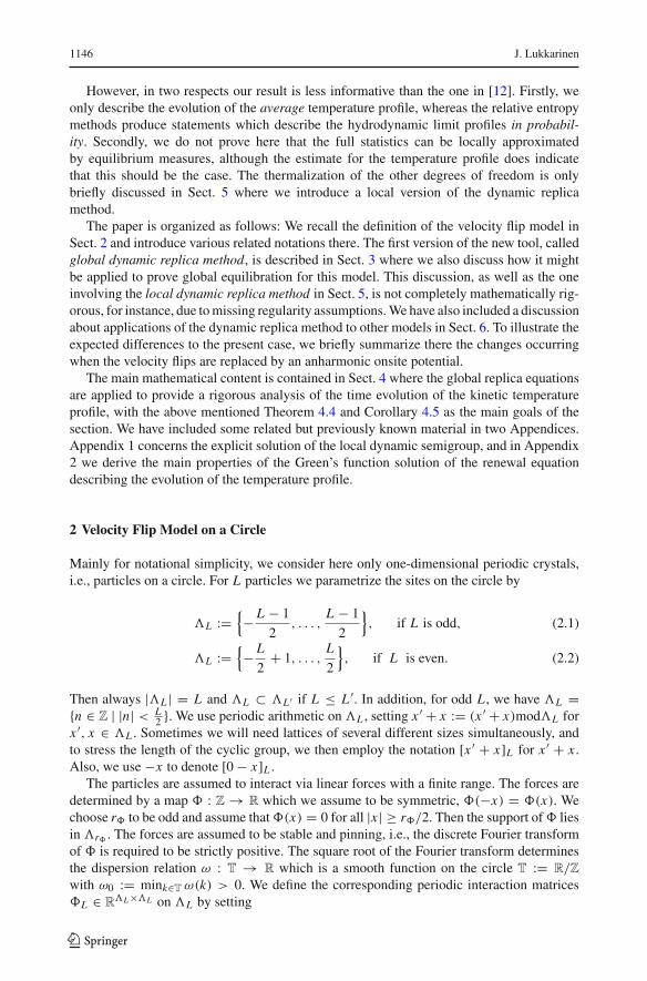
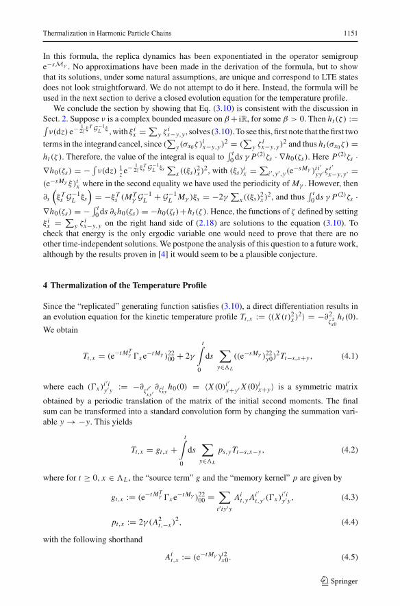
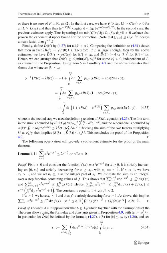
Fig. 1 Plots of the function I (k0) defined by the left hand side of the nondegeneracy condition in (4.8)for γ = 6 and two different dispersion relations. The left plot is for the standard nearest neighbor case,ω(k) =
√1 + 4 sin2(πk), while the right one depicts a degenerate next-to-nearest neighbor case, withω(k) =√
1 + 4 sin2(2πk). The plots have been generated by numerical integration using Mathematica
exponential bounds for the errors from diffusive evolution of the temperature profile. Thisrequires to rule out resonant behavior, which can be achieved if the noise flipping rate is highenough and the dispersion relation satisfies a certain integral bound excluding degeneratebehavior. Explicitly, we only consider γ and � satisfying the following:
Assumption 4.3 Suppose that � satisfies the assumptions in 4.1, and γ > 0 is given suchthat:
1. (noise dominates) γ 2 > 4 maxk �(k).2. (harmonic forces are nondegenerate) For any ε > 0 there is Cε > 0 such that
∞∫
0
dt∫
T
dk
(A2
t
(k + k0
2
)− A2
t
(k − k0
2
))2
≥ Cε, whenever ε ≤ |k0| ≤ 1
2. (4.8)
The nondegeneracy condition is satisfied by the nearest neighbor interactions, for which
ω(k) =√ω2
0 + 4 sin2(πk) with ω0 > 0. This can be proven for instance by relying on the
estimate ∂k A2t (k) ≥ Cte−tγ sin(2πk) valid for all |k| < 1/2 and large enough t . However,
the condition fails for the degenerate next-to-nearest neighbor coupling which skips over
the nearest neighbors: then ω(k) =√ω2
0 + 4 sin2(2πk) and thus for k0 = 1/2 we haveω(k +k0/2) = ω(k −k0/2) for all k, hence the integral in (4.8) evaluates to zero at k0 = 1/2.Instead of including a formal proof of these statements, we have depicted the values of theabove integrals for one choice of parameters in Fig. 1.
We prove in this section that these assumptions suffice to have the following pointwisebehavior of the temperature profile.
Theorem 4.4 Suppose � and γ satisfy the conditions in Assumption 4.3. Then there isL0 ∈ N such that Eq. (4.2) has a unique continuous solution Tt,x for every L ≥ L0 wheneverall second moments of the initial field X (0) exist. Let E := |�L |−1〈HL(X)〉 < ∞ denote thetotal energy density. Then there are constants C, d > 0, independent of the initial data andof L, such that for this solution
∣∣Tt,x − E∣∣ ≤ CE e−dt L−2
1 − e−2dt L−2 , (4.9)
123
1154 J. Lukkarinen
for all t ≥ 0 and x ∈ �L . In addition, we can choose C and define τx ∈ R and px ≥ 0,x ∈ �L , so that for all t > 0 and x ∈ �L
∣∣∣Tt,x − (e−t Dτ)x
∣∣∣ ≤ CELt−3/2, (4.10)
where the operator D is defined by
(Dτ)x :=∑
y∈�L
py(2τx − τx+y − τx−y
), x ∈ �L . (4.11)
Both τx and px in the statement have explicit definitions which can be found in the beginningof the proof of the Theorem. To summarize in words, the first of the bounds implies thatthe temperature profile equilibrates, and the relative error is exponentially decaying on thediffusive time scale, i.e., as t L−2 becomes large. The second statement says that solvingthe “lattice diffusion equation” ∂Tt,x = −(DTt )x with initial data T0 = τ provides anapproximation to the temperature profile which is accurate even before the diffusive timescale, for t � L2/3.
A closer inspection of the proof of the Theorem reveals that the main contribution to theerror bound given in (4.10) comes from “memory effects” of the original time evolution. Thesecorrections can estimated using a bound which for large t and L behaves as
∫∞−∞ dk k2e−tk2 =
O(t−3/2). The rest of the factors can be uniformly bounded using the total energy, resultingin the bound in (4.10). We do not know if the bound is optimal, although this could well betrue for generic initial data. The worst case scenario for thermalization should be given byinitial data in which all energy is localized to one site. It would thus be of interest to studythe solution of (4.2) with initial data q(0)x = 0 and p(0)x = √
2L 1(x=0) in more detail tosettle the issue.
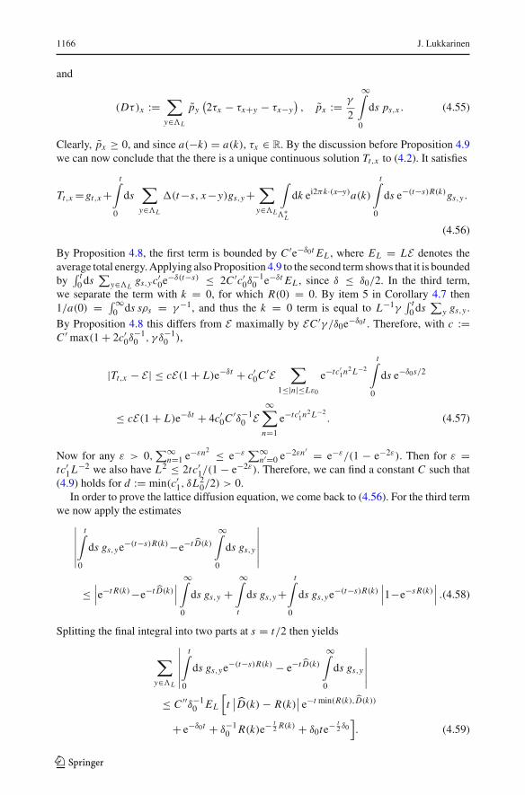
The following corollary makes the connection to diffusion more explicit. Its physicalmotivation is to show that the Fourier’s law can here be used to predict results from temper-ature measurements, as soon as these are not sensitive to the lattice structure. Explicitly, weassume that the measurement device detects only the cumulative effect of thermal movementof the particles, say via thermal radiation, and thus can only measure a smeared temperatureprofile. The smearing is assumed to be linear and given by a convolution with some fixedfunction ϕ which for convenience we assume to be smooth and rapidly decaying, i.e., that itshould belong to the Schwartz space. The Corollary implies that then for large systems it ispossible to obtain excellent predictions for future measurements of the temperature profileby first waiting a time t0 � L2/3, measuring the temperature profile, and then using theprofile as initial data for the time-dependent Fourier’s law. The diffusion constant κL of theFourier’s law depends on the harmonic dynamics and is given by (4.14) below. We provelater, in Corollary 4.7 and Proposition 4.9, that the constant remains uniformly bounded awayfrom 0 and infinity. Hence, the present assumptions are sufficient to guarantee normal heatconduction. We have also computed the values of κL numerically for a nearest neighborhoodinteraction and plotted these in Fig. 2. The results indicate that the limit L → ∞ exists and
agrees with κ∞ = γ−1/(2 + ω20 + ω0
√ω2
0 + 4) which is the value obtained in previousworks on this model [8,9,12].
Corollary 4.5 Suppose the assumptions of Theorem 4.4 hold, L ≥ L0, and all secondmoments of the initial field exist. Let Tt,x denote the corresponding solution to (4.2) andE := |�L |−1〈HL 〉 the energy density. For any kernel function ϕ ∈ S(R) and initializationtime t0 > 0, define the corresponding observed temperature profile by
123
Thermalization in Harmonic Particle Chains 1155
5 10 15 20
0.01
0.02
0.03
0.04
0.05
Fig. 2 Plot of κL for nearest neighbor interactions with ω0 = 1 and using γ = 6 for L = 2, 3, . . . , 20. Thehorizontal line depicts the corresponding predicted infinite volume value κ∞, as explained in the text
T (obs)(t, ξ) :=∑y∈Z
ϕ(ξ − y)Tt0+t,y mod �L, t ≥ 0, ξ ∈ LT. (4.12)
Let the predicted temperature profile be defined as the solution of the diffusion equation onthe circle LT with initial data T (obs)(0, ·), i.e., let T (pred) ∈ C (2)([0,∞) × LT) be theunique solution to the Cauchy problem
∂t T(pred)(t, ξ) = κL ∂
2ξ T (pred)(t, ξ) , T (pred)(0, ξ) = T (obs)(0, ξ) (4.13)
where t ≥ 0 and ξ ∈ LT, and the diffusion constant is defined by
κL :=∑
y∈�L
y2 py > 0. (4.14)
Then there is a constant C > 0, independent of the initial data and of L, ϕ and t0, such that∣∣∣T (pred)(t, ξ)−T (obs)(t, ξ)
∣∣∣≤CELt−3/20
(‖ϕ‖1+sup
ξ
∑y∈Z
|ϕ(ξ − y)|)+CE
∑|n|≥L/2
|ϕ(n/L)| ,
(4.15)
for all t ≥ 0 and ξ ∈ LT. In particular, if ϕ is a “macroscopic averaging kernel” andsatisfies additionally ϕ ≥ 0,
∫R
dx ϕ(x) = 1 and ϕ(p) = 0 for all |p| ≥ 12 , then for the same
C as above ∣∣∣T (pred)(t, ξ)− T (obs)(t, ξ)∣∣∣ ≤ 2CELt−3/2
0 . (4.16)
The rest of this section is used for proving the above statements. However, as the argumentsget somewhat technical and will not be used in the remaining sections, it is possible to skipover the details in the first reading. We begin with a Lemma collecting the main consequencesof our assumptions.
Lemma 4.6 Suppose � and γ satisfy the conditions in Assumption 4.3. Use (4.6) to defineAi : [0,∞) × T → R for i = 1, 2, and set δ0 = ω2
0/γ . Then we can find constantsc0, c1, c2, γ2 > 0, t1 ≥ 0, such that
1. The functions Ai , i = 1, 2, belong to C (1)([0,∞)× T).
123
1156 J. Lukkarinen
2. | Ait (k)|, |∂t Ai
t (k)| ≤ c0e−δ0t and |∂k Ait (k)| ≤ c0e−δ0t/2 for every i = 1, 2, t ≥ 0 and
k ∈ T.3. − A2
t (k) ≥ c1e−γ t/2 for all t ≥ t1 and k ∈ T.4. The functions Ai
t,x := ∫T
dk ei2πx ·k Ait (k), x ∈ Z, satisfy | Ai
t,x | ≤ c2e−δ0t/2−γ2|x | for alli = 1, 2, t ≥ 0, x ∈ Z.
Proof The first item follows straightforwardly from the definitions. As in the state-ment, set δ0 := ω2
0/γ > 0 and recall the functions u and μ± defined in (4.7). Sinceω(k)2/μ+(k) = μ−(k) < μ+(k) ≤ γ , we have μ+(k) > μ−(k) ≥ δ0 for all k andthus a direct computation shows that c0 for the first two upper bounds in item 2 can befound. The bound for |∂k Ai
t (k)| follows similarly, using the estimate te−tδ0/2 ≤ e−12/δ0
and possibly increasing c0 to accommodate the extra factors resulting from taking thederivative, such as maxk |ω′(k)| < ∞. The lower bound in item 3 is a direct conse-quence of the identity − A2
t (k) = (2u)−1μ−e−tμ− (1 − e−t2uμ+/μ−)
where u = u(k) ≥u0 :=
√(γ /2)2 − maxk �(k) > 0 and μ− ≤ γ /2. (We may define, for instance,
t1 := (2u0)−1 ln(2γ 2/ω2
0) and c1 := ω20/(2γ
2).)All of the maps k → Ai
t (k) can be represented as a composition of a function analyticon C \ {0} and the function u (note that ω(k)2 = (γ /2)2 − u(k)2). Then, by assumption,
0 < u0 ≤ u(k) ≤√(γ /2)2 − ω2
0 ≤ 12γ − δ0 for real k, and there is a strip on which
(γ /2)2 − ω(z)2 is an analytic, 1-periodic function. Therefore, we can find ε0 > 0 such thatu(z) is an analytic, 1-periodic continuation of u to a neighborhood of U := R + i[−ε0, ε0]with u0/2 ≤ Re u(z) ≤ 1
2γ − δ0/2. Hence, Ait |u→u(z) is also analytic and 1-periodic on U
and it is bounded there by 4u−10 (1 + (γ /2)2 + maxz∈U |u(z)|2)e−δ0t/2 for i = 1, 2, t ≥ 0.
Therefore, Cauchy’s theorem can be used to change the integration contour in the definitionof Ai
t,x from [−1/2, 1/2] to [−1/2, 1/2] + i sign(x)ε0 without altering the value of theintegral. Thus we can define γ2 := 2πε0 and find c2 > 0 independent of x, t, i such that| Ai
t,x | ≤ c2e−δ0t/2−γ2|x | for all i = 1, 2, t ≥ 0, x ∈ Z. This concludes the proof of theLemma. ��
Corollary 4.7 Suppose � and γ satisfy the conditions in Assumption 4.3 and let δ0, γ2, t1be constants for which Lemma 4.6 holds. For each L ≥ 1 define
pt,x := 2γ
⎛⎜⎝∫
�∗L
dk e−i2πk·x A2t (k)
⎞⎟⎠
2
, ρt :=∑
y∈�L
pt,y, (4.17)
for t ≥ 0 and x ∈ �L . Then there are constants C0,C1,C2 > 0, all independent of L, suchthat
1. t → pt,x belongs to C (1)([0,∞)) for all x ∈ �L .2. pt,−x = pt,x for all x, t .3. pt,x ≥ 0 and |∂t pt,x |, pt,x ≤ C0e−γ2|x |−δ0t for all x ∈ �L and t ≥ 0.4.∫∞
0 dt∑
x∈�Lpt,x = 1.
5.∫∞
0 dt∑
x∈�Ltpt,x = γ−1.
6. 0 ≤ ρt ≤ C1e−2δ0t , for all t , and ρt ≥ C2e−γ t for t ≥ t1.
Proof The first item follows directly from the corresponding item in Lemma 4.6. Considerthen a fixed L ≥ 1 and denote A2
t,x := ∫�∗
Ldk ei2πk·x A2
t (k) for x ∈ �L , t ≥ 0. Since
123
Thermalization in Harmonic Particle Chains 1157
A2t (k) ∈ R with A2
t (−k) = A2t (k), we have A2
t,x ∈ R with A2t,−x = A2
t,x . Hence, pt,−x = pt,x
and pt,x ≥ 0. In particular, item 2 holds.By Lemma 4.6, the Fourier-transform of A2
t (k), denoted A2t,x , is absolutely summable,
and thus A2t (k) = ∑
y∈Ze−i2πy·k A2
t,y for every k ∈ T. Inserting the formula in the definition
of A2t,x yields
A2t,x =
∑n∈Z
A2t,x+nL , (4.18)
for all x, t . In the above sum, the definition of�L implies that |x +nL| ≥ L(|n|−1)+L/2 ≥L(|n| − 1) + |x | if n �= 0. The exponential bound in item 4 of Lemma 4.6 thus shows that|A2
t,x | ≤ c2e−δ0t/2−γ2|x |(1 + 2/(1 − e−γ2 L)). As mentioned above, A2t,x ∈ R and thus 0 ≤
we find using item 2 in Lemma 4.6 that |∂t pt,x | ≤ 4γ c0c2(1 + 2/(1 − e−γ2))e−δ0t3/2−γ2|x |.Choosing C0 := 4γ c0c2(1 + 2/(1 − e−γ2)) thus implies that item 3 holds.
Using the discrete Parseval’s theorem in the definition of ρt yields an alternative repre-sentation ρt = 2γ
∫�∗
Ldk ( A2
t (k))2. Hence, the bounds in Lemma 4.6 imply that the bounds
in item 6 hold for the choices C1 := 2γ c20 and C2 := 2γ c2
1. A direct computation usingthe definition of A2
t (k) shows that∫∞
0 dt ( A2t (k))
2 = (2γ )−1 independently of k. Therefore,∫∞0 dt
∑x pt (x) = ∫∞
0 dtρt = 1 and item 4 holds. The equality∫∞
0 dt∑
x∈�Ltpt,x = γ−1
can be checked analogously. This concludes the proof of the Corollary. ��The normalization in item 4 is a crucial identity which makes the structure of (4.2) to
be that of a renewal equation. Instead of the explicit computation referred to in the aboveproof, the identity can also be inferred by noting that the integral is equal to a (2, 2)-diagonal
component of∫∞
0 dt e−t MTγ
(0 00 1
)e−t Mγ . By the results proven in [6] the integral yields G−1
L ,
and thus its (2, 2)-component has only ones on the diagonal.The main properties of the “source term”, gt,x , are summarized in the following Proposi-
tion.
Proposition 4.8 Suppose�andγ satisfy the conditions in Assumption 4.3 and let δ0 = ω20/γ
as in Lemma 4.6. If L ≥ 1 and all second moments of the initial field X (0) exist, we definefor t ≥ 0 and x ∈ �L
gt,x :=∑
i ′,i=1,2
∑y′,y∈�L
Ait,y Ai ′
t,y′ 〈X (0)i′
x+y′ X (0)ix+y〉, (4.19)
where A2t,x := ∫
�∗Ldk ei2πk·x Ai
t (k). Then there is a constant C ′, independent of L and the
choice of initial state, such that all of the following statements hold with EL := 〈HL(X (0))〉 <∞:
1. gt,x ≥ 0 for all t, x.2.∑
x gt,x ≤ C ′e−δ0t EL for all t .3.∫∞
0 dt∑
x∈�Lgt,x = γ−1 EL .
Proof The assumptions imply that Lemma 4.6 holds. In the following, the constantsc0, c1, c2, γ2, t1 refer to those appearing in the Lemma.
Since it follows from the definition that gt,x = 〈(∑i,y Ait,y X (0)ix+y)
2〉, obviously gt,x ≥0. As in the proof of Corollary 4.7, Lemma 4.6 implies that now |Ai
t,y | ≤ c2e−δ0t/2−γ2|y|(1+
123
1158 J. Lukkarinen
2/(1−e−γ2)). By the Schwarz inequality∑
i ′,i,x 〈|X (0)i′
x+y′ X (0)ix+y |〉 ≤ 2〈‖X (0)‖22〉. Since
‖X‖22 ≤ HL(X)2/min(1, ω2
0), we find that item 2 holds for C ′ = 4c22 max(1, ω−2
0 )(1 +2/(1−e−γ2))4.
For the final item, we return to the matrix formulation of g. Since Ait,y−x = (e−t Mγ )i2
yx
by periodicity, we have gt,x = 〈((e−t MTγ X (0))2x )
2〉 and thus
∑x∈�L
gt,x = 〈X (0)T e−t Mγ P(2)e−t MTγ X (0)〉, where P(2) :=
(0 00 1
). (4.20)
Therefore,∫∞
0 dt∑
x∈�Lgt,x = 〈X (0)T Q X (0)〉 where Q := ∫∞
0 dt e−t Mγ P(2)e−t MTγ is the
unique real symmetric matrix satisfying Mγ Q + QMTγ = P(2). Using the definition of Mγ
in (3.6), we can then verify that Q = 12γ
(�L 00 1
). Thus X T Q X = HL(X)/γ , and we can
conclude that item 3 holds. ��Renewal equations can conveniently be studied via Laplace transforms. We have included
a proof in Appendix 2 how the above bounds allow for an explicit representation of thesolution of (4.2) for any continuous “initial data” gt,x . The solution is also unique, at least inthe class of continuous functions. We denote the solution by Tt,x and conclude that
Tt,x = gt,x +t∫
0
ds∑
y∈�L
G(t − s, x − y)gs,y, (4.21)
where for any ε > 0
G(t, x) := pt,x +∫
�∗L
dk ei2πk·xε+i∞∫
ε−i∞
dλ
2π ieλt p(λ, k)2
1 − p(λ, k), (4.22)
and p(λ, k) := ∫∞0 ds
∑y∈�L
ps,ye−sλe−i2πk·y is analytic for Re λ > −δ0. The estimatesproven in Proposition 8.1 also imply that | p(λ, k)| ≤ C ′/(1 +|λ|) for all k if Re λ ≥ −δ0/2,where C ′ can be chosen independently of L . In particular, the above integral is absolutelyconvergent for any choice of ε > 0.
Many of the properties below could be derived more easily by relying on standard results,such as the implicit function theorem. However, for such bounds to be useful here, it is crucialto obtain them with L-independent constants. To convince the reader that no L-dependenceis sneaking in, we provide here detailed estimates with examples of such L-independentconstants albeit at the cost of some repetition of standard computations. No claim is madethat the given choices for the constants would be optimal.
Proposition 4.9 Suppose � and γ satisfy the conditions in Assumption 4.3, and set δ0 =ω2
0/γ . Then we can find constants c′0, δ, ε0, β > 0 and L0 ≥ 1, such that β ≤ δ0/2 and for
all L ≥ L0, x ∈ �L , t ≥ 0,
G(t, x) =∫
�∗L
dk ei2πk·x a(k)e−t R(k) +�(t, x), (4.23)
where
|�(t, x)| ≤ c′0e−δt . (4.24)
123
Thermalization in Harmonic Particle Chains 1159
Here a(k) and R(k) are defined for |k| > ε0 by a(k) = 0 and R(k) = β, and for |k| ≤ ε0
there is a unique R(k) ∈ [0, β], such that
1 =∞∫
0
ds es R(k)∑
y∈�L
ps,y cos(2πk · y), (4.25)
and then
1
a(k)=
∞∫
0
ds ses R(k)∑
y∈�L
ps,y cos(2πk · y). (4.26)
In addition, we can choose the constants so that there are c′1, c′
2, c′3, c′
4, κ′ > 0, all indepen-
dent of L, such that for all L ≥ L0 and k ∈ �∗L with |k| ≤ ε0 all of the following estimates
hold:
1. 0 < a(k) ≤ c′0.
2.∫∞
0 ds∑
y∈�Ly2 ps,y ≥ κ ′.
3. c′1k2 ≤ R(k) ≤ c′
2k2 and |D(k; L)− R(k)| ≤ c′4k4 with
D(k′; L) := γ∑
y∈�L
(1 − cos(2πk′ · y))
∞∫
0
ds ps,y, k′ ∈ �∗L . (4.27)
In addition, we may assume D(k′; L) ≥ c′3 min(|k′|, ε0)
2 for all k′ ∈ �∗L .
Proof The goal is to use Cauchy’s theorem to move the integration contour in (4.22) to theleft half-plane, in which case the factor eλt produces exponential decay in time. To do this,it is crucial to study the zeroes of 1 − p since these will correspond to poles of the integranddetermining the dominant modes of decay. For notational simplicity, let us for the momentconsider some fixed k0 ∈ �∗
L and set F(λ) := 1 − p(λ, k0). As proven in Appendix 2,| p(λ, k0)| < 1 if Re λ > 0 and thus F is an analytic function for Re λ > −δ0 which has nozeroes in the right half plane. It turns out that under the present assumptions, in particular,when the nondegeneracy condition in Assumption 4.3 holds, only the case with small k0 andλ will be relevant, and we begin by considering that case.
Suppose first that λ, λ0 ∈ C with Re λ,Re λ0 > −δ0, and n ∈ N, with n = 0 also allowed.The derivatives of p can be computed by differentiating the defining integrand. Therefore,the nth derivative of F is equal to 1(n = 0)+ (−1)n+1
∫∞0 ds
∑y∈�L
ps,ysne−sλe−i2πk0·y .Thus by item 6 in Corollary 4.7, for any n ≥ 0, we have
|F (n)(λ)− F (n)(λ0)| ≤∞∫
0
ds ρssn |e−sλ0 − e−sλ|
≤ |λ− λ0|C1
∞∫
0
ds sn+1e−δ0s = |λ− λ0|n!C1δ−(n+2)0 . (4.28)
Here, the second bound can be derived for instance from the representation e−sλ0 − e−sλ =∫ 10 dr s(λ − λ0)e−s(λ+r(λ0−λ)) where in the exponent for any r the real part is bounded byδ0s. Since pt,−y = pt,y , we also have
F ′(0) =∞∫
0
ds∑
y∈�L
sps,y cos(2πk0 · y) =∞∫
0
ds sρs −∞∫
0
ds∑
y∈�L
sps,y2 sin2(πk0 · y)
123
1160 J. Lukkarinen
≥ C2
∞∫
t1
ds se−γ s − 2π2|k0|2∞∫
0
ds∑
y∈�L
y2sps,y
≥ C2(1 + γ t1)γ−2e−γ t1 − 4π2|k0|2C0δ
−20
∞∑n=1
n2e−γ2n, (4.29)
where we have used that | sin x | ≤ |x |, for any x ∈ R, and applied the bounds in Corollary4.7. Here the constants b0 := C2(1 + γ t1)γ−2e−γ t1 and C4 := 4π2C0δ
−20
∑∞n=1 n2e−γ2n
are strictly positive and independent of L . Therefore, so is ε1 := √b0/(2C4) and we can
conclude that whenever |k0| ≤ ε1, we have F ′(0) ≥ b0/2.Consider then the case |k0| ≤ ε1, with ε1 > 0 defined above. Let r0 > 0 be given
such that r0 < δ0 and suppose that λ satisfies |λ| ≤ r0. Then F ′(0) ≥ b0/2 and by (4.28)we have |F ′(λ) − F ′(0)| ≤ r0C1δ
−30 . Hence, Re F ′(λ) ≥ b0/2 − r0C1δ
−30 . We set r0 :=
min(δ0/2, b0δ30/(4C1)) which is L-independent and strictly positive, and conclude that then
we have a lower bound Re F ′(λ) ≥ b0/4 > 0 for all |λ| ≤ r0. On the other hand, if|λ|, |λ0| ≤ r0 withλ �= λ0, then the identity F(λ) = F(λ0)+(λ−λ0)
∫ 10 dr F ′(λ0+r(λ−λ0))
implies a bound
ReF(λ)− F(λ0)
λ− λ0≥ b0
4> 0. (4.30)
Suppose that λ0 is a zero of F in the closed ball of radius r0. Since Re F ′(λ0) > 0, then λ0 hasmultiplicity one. Also, by (4.30), we have |F(λ)| ≥ |λ − λ0|b0/4 for all |λ| ≤ r0, and thusthere can then be no other zeros of F in the ball. Since F(λ∗) = F(λ)∗ and F(r) > 0 for allr > 0, we can also conclude that then necessarily λ0 = −R0 with 0 ≤ R0 ≤ r0. Therefore,if λ = −β + iα, with β �= R0, 0 ≤ β ≤ r0/2 and α is real and satisfies |α| ≤ r0/2, we mayalways use the estimate |1/F(λ)| ≤ 4b−1
0 /|R0 − β|.
Consider then the case in which there are no zeros of F in the closed ball of radius r0.The map r → F(r) is continuous, it maps real values to real values, and F(r0) > 0. Hencenow F(−r) > 0 for all 0 ≤ r ≤ r0. We apply (4.30) with λ0 = −r0 to conclude that for all|λ| ≤ r0 with λ �= −r0
ReF(λ)
λ+ r0≥ b0
4+ Re
F(−r0)
λ+ r0≥ b0
4> 0. (4.31)
Therefore,
|F(λ)| ≥ |λ+ r0|∣∣∣∣Re
F(λ)
λ+ r0
∣∣∣∣ ≥ |λ+ r0|b0
4. (4.32)
We can then conclude that |1/F(λ)| ≤ 8/(r0b0) whenever λ = −β + iα with 0 ≤ β ≤ r0/2and α is real and satisfies |α| ≤ r0/2.
The above estimates are sufficient to control the r0-neighborhood of zero for small k0.Coming back to general k0 we next study the properties of F on the imaginary axis, forλ = iα with α ∈ R. Using item 4 in Corollary 4.7 and the notations introduced in the proofof the Corollary shows that
123
Thermalization in Harmonic Particle Chains 1161
Re F(iα) =∞∫
0
ds∑
y∈�L
ps,y (1 − cos(sα + 2πk0 · y))
= 4γ
∞∫
0
ds∑
y∈�L
∣∣∣∣A2s,ysin
(1
2sα + πk0 · y
)∣∣∣∣2
= 4γ
∞∫
0
ds∫
�∗L
dk
∣∣∣∣∣∣∑
y∈�L
e−i2πk·y A2s,y sin
(1
2sα + πk0 · y
)∣∣∣∣∣∣
2
. (4.33)
Since k0 ∈ �∗L , there is n0 ∈ �L such that k0 = n0/L . To derive lower bounds for (4.33), it
suffices to consider the case in which n0 ≥ 0, since then for n0 < 0 we can use the symmetryof cosine and apply the bounds derived for the case where the signs of α and k0 are reversed.
Consider first the case in which n0 is even. Then there is n1 ∈ �L such that 0 ≤ n1 ≤ L/4and n0 = 2n1. In this case, k0/2 ∈ �∗
L , the Fourier-transform of y → A2s,y equals A2
s (k)
and thus by using sin x = (eix − e−ix )/(2i) in (4.33) yields
Re F(iα) = γ
∞∫
0
ds∫
�∗L
dk∣∣eisα/2 A2
s (k − k0/2)− e−isα/2 A2s (k + k0/2)
∣∣2
≥ γ
∞∫
t1
ds∫
�∗L
dk(
A2s (k − k0/2)− A2
s (k + k0/2))2
+ 2γ
∞∫
t1
ds (1 − cos(sα))∫
�∗L
dk A2s (k − k0/2) A
2s (k + k0/2) (4.34)
where in the last step we used the fact that A2s are real. Applying the lower bound in item 3
of Lemma 4.6 thus proves that
Re F(iα) ≥ 2γ
∞∫
t1
ds (1 − cos(sα))c21e−γ s . (4.35)
For instance by representing the cosine as a sum of two exponential terms, we find that∫∞t ds (1 − cos(sα))e−γ s = γ−1e−γ tα2/(α2 + γ 2) if |α|t ∈ 2πZ. Therefore, now
Re F(iα) ≥ 2c21e−γ t1 e−2π |γ /α| 1
1 + |γ /α|2 . (4.36)
For any r > 0, set C(r) to be equal to the right hand side at α = r . Then C(r) > 0, it isindependent of L , and we can conclude that Re F(iα) ≥ C(r) whenever |α| ≥ r and Lk0 iseven.
In the remaining cases n0 is odd and positive. Then there is n1 ∈ �L such that 0 ≤n1 ≤ L/4 and n0 = 2n1 + 1. Thus we can apply the above estimate for Re F(iα) atk0 − 1/L = 2n1/L . On the other hand,
and we can conclude that for odd n0 and every |α| ≥ r > 0
Re F(iα) ≥ C(r)−∞∫
0
ds∑
y∈�L
ps,y2π |y|
L≥ C(r)− L−1 4πC0
δ0
∞∑n=1
ne−γ2n, (4.38)
where in the second inequality we have applied the bounds in item 3 of Corollary 4.7.Therefore, to every r > 0 there is L(r) ∈ N+ such that the final bound is greater thanC(r)/2 for every L ≥ L(r). Thus we can conclude that, if r > 0 and L ≥ L(r), thenRe F(iα; k0, L) ≥ C(r)/2 for all |α| ≥ r and k0 ∈ �∗
L .If β satisfies 0 ≤ β < δ0, then by (4.28) we have |F(−β + iα)− F(iα)| ≤ βC1δ
−20 for
all real α. Therefore, if we set β(r) := 12 δ0 min(1, C(r)δ0/(2C1)) for r > 0, then we have
found strictly positive, L-independent constants such that for any r > 0 and L ≥ L(r)
Re F(−β + iα; k0, L) ≥ 1
4C(r) > 0, (4.39)
for all k0 ∈ �∗L , |α| ≥ r , and 0 ≤ β ≤ β(r) ≤ δ0/2.
It is now possible to conclude the estimates for the case when |k0| ≤ ε1. Recall the earlierdefinition of r0 and set C5 := C(r0/2), L5 := L(r0/2) and β1 := β(r0/2). Assume thatL ≥ L5. We use Cauchy’s theorem and, when necessary, the residue theorem to change theintegration contour from ε′ + iR, ε′ > 0, to −β + iR with some β > 0. If there are nozeroes of F in the closed ball of radius r0, we choose β = β0 with β0 := min(β1, r0/2) andthe above results imply that the integrand in (4.22) is analytic for Re λ ≥ −β0 and we have|1/F | ≤ max(4/C5, 8/(r0b0)) on the integration contour. If there are zeroes in the ball, thenthe zero is unique and lies at −R0 with 0 ≤ R0 ≤ r0 and 1/F has a first order pole at −R0. IfR0 > β0/2, we choose β = β0/4 < β1 when the integrand is analytic to the right of the finalcontour and hence the pole does not contribute. Then also |1/F | ≤ max(4/C5, 16/(β0b0))
on the integration contour. If R0 ≤ β0/2, we choose β = β0. Then the residue theorem canbe used to evaluate the contribution from the pole, and the remaining integral over −β + iRcan be bounded using |1/F | ≤ max(4/C5, 8/(β0b0)).
Assume then that L ≥ L5 and |k0| ≤ ε1. Following the above steps, we find that, if thereis 0 ≤ R0 ≤ β0/2 such that
1 =∞∫
0
ds es R0∑
y∈�L
ps,ycos(2πk0 · y), (4.40)
then p(−R0, k0) = 1 and
ε′+i∞∫
ε′−i∞
dλ
2π ieλt p(λ, k0)
2
1 − p(λ, k0)= 1
m(k0)e−t R0 +�. (4.41)
Here m(k0) = F ′(−R0), implying
m(k0) :=∞∫
0
ds ses R0∑
y∈�L
ps,y cos(2πk0 · y) ≥ b0
4> 0, (4.42)
and there is a constant C6 > 0, independent of L , such that
|�| ≤ C6e−β0t . (4.43)
123
Thermalization in Harmonic Particle Chains 1163
(Recall that | p(λ, k0)| ≤ C ′/(1 + |λ|) for Re λ ≥ −δ0/2.) If no such R0 can be found, thenp(−r, k0) < 1 for all r ≤ β0/2 and one of the remaining cases is realized. Hence, then
∣∣∣∣∣∣∣
ε′+i∞∫
ε′−i∞
dλ
2π ieλt p(λ, k0)
2
1 − p(λ, k0)
∣∣∣∣∣∣∣≤ C ′
6e−β0t/4, (4.44)
with some L-independent C ′6 > 0.
The following Lemma will be used to study the remaining values of k0.
Lemma 4.10 Suppose Assumption 4.3 holds. Then for every ε > 0 we can find C(ε) > 0,L(ε) ∈ N+ and β(ε) ∈ (0, δ0/2] such that, if L ≥ L(ε) and k0 ∈ �∗
L with |k0| ≥ ε, thenF(0; k0, L) ≥ C(ε) and Re F(λ; k0, L) ≥ C(ε)/2 for all λ with 0 ≥ Re λ ≥ −β(ε).Proof Fix ε > 0 and let Cε > 0 denote the corresponding constant in Assumption 4.3. Asproven above, if L ≥ 1 and k0 ∈ �∗
L is such that Lk0 is a even and nonnegative, then
F(0; k0, L) = γ
∞∫
0
ds∫
�∗L
dk fs(k, k0), fs(k, k0) := (A2
s (k − k0/2)− A2s (k + k0/2)
)2.
(4.45)
If h ∈ C (1)(T), then | ∫T
dk h(k) − ∫�∗
Ldk h(k)| ≤ ∑
n∈�L‖h′‖∞
∫|k−n/L|≤(2L)−1 dk |k −
n/L| ≤ ‖h′‖∞/(2L). By Lemma 4.6, we can apply this in the above with ‖h′‖∞ ≤ 8c20e−δ0s .
Therefore,∣∣∣∣∣∣F(0; k0, L)− γ
∞∫
0
ds∫
T
dk fs(k, k0)
∣∣∣∣∣∣≤ 4γ c2
0
Lδ0. (4.46)
If Lk0 is odd and nonnegative, we have by (4.37)
|F(0; k0, L)− F(0; k0−1/L , L)| ≤ 4πC0
Lδ0
∞∑n=1
ne−γ2n (4.47)
and also | fs(k, k0) − fs(k, k0−1/L)| ≤ 4c20e−δ0s L−1, by Lemma 4.6. Therefore, there is
an L-independent constant C > 0 such that∣∣F(0; k0, L)− γ
∫∞0 ds
∫T
dk fs(k, k0)∣∣ ≤ C/L
for all k0 ∈ �∗L . If |k0| ≥ ε, then by assumption γ
∫∞0 ds
∫T
dk fs(k, k0) ≥ γCε and henceF(0; k0, L) ≥ γCε − C/L . Thus by choosing L ′(ε) such that L ′(ε) ≥ 2C/(γCε) we haveF(0; k0, L) ≥ γCε/2 whenever L ≥ L ′(ε) and |k0| ≥ ε.
Consider then some fixed L ≥ L ′(ε) and |k0| ≥ ε. By the earlier results, |F(λ)− F(0)| ≤rC1δ
−20 if |λ| ≤ r < δ0. (The constant C1 here should not be confused with Cε at ε = 1.)
Thus if r1 := min(δ0/2, γCεδ20/(4C1)) > 0, then Re F(λ) ≥ γCε/4 for all |λ| ≤ r1. On
the other hand, if also L ≥ L(r1/2), then we have Re F(−β + iα) ≥ C(r1/2)/4 for all0 ≤ β ≤ β(r1/2) and |α| ≥ r1/2. Combining the above estimates yields constants such thatthe Lemma holds for all L ≥ L(ε) := max(L ′(ε), L(r1/2)). ��
We next apply Lemma 4.10 with ε = ε1/2 > 0. Set thus L7 := L(ε1/2), C7 := C(ε1/2),and β2 := β(ε1/2). Assume L ≥ L7 and k0 ∈ �∗
L with |k0| ≥ ε1/2. Then by the Lemma,for any λ = −β + iα, with 0 ≤ β ≤ β2 and α ∈ R we have |1/F(λ)| ≤ 2/C7. Therefore,
123
1164 J. Lukkarinen
we can change the contour to −β2 + iR without encountering any singularities. This provesthat there is an L-independent constant C8 such that for |k0| ≥ ε1 and L ≥ L7∣∣∣∣∣∣∣
ε′+i∞∫
ε′−i∞
dλ
2π ieλt p(λ, k0)
2
1 − p(λ, k0)
∣∣∣∣∣∣∣≤ C8e−β2t . (4.48)
Collecting the above estimates together proves that there are constants c′0 > 0, β ′ > 0,
L ′ ∈ N+, such that if L ≥ L ′, then for all k0 ∈ �∗L either
∣∣∣∣∣∣∣
ε′+i∞∫
ε′−i∞
dλ
2π ieλt p(λ, k0)
2
1 − p(λ, k0)
∣∣∣∣∣∣∣≤ c′
0e−β ′t , (4.49)
or |k0| ≤ ε1 and there are R(k0) and a(k0) := 1/m0(k0) satisfying (4.25) and (4.26) suchthat ∣∣∣∣∣∣∣
ε′+i∞∫
ε′−i∞
dλ
2π ieλt p(λ, k0)
2
1 − p(λ, k0)− a(k0)e
−t R(k0)
∣∣∣∣∣∣∣≤ c′
0e−β ′t . (4.50)
We still need to make sure that all the claimed bounds will hold. From now on we assumethat L ≥ L ′ so that all of the earlier derived bounds can be used. Suppose then that |k0| ≤ ε1.Since F(−R) ∈ R, for 0 ≤ R ≤ r0, (4.30) implies that F(−R) ≤ F(0) − Rb0/4 for theseR. Therefore, if F(−R(k0)) = 0, we have 0 ≤ R(k0) ≤ 4F(0)/b0. Since
F(0)=2
∞∫
0
ds∑
y∈�L
ps,ysin2(πk0 · y) ≤ 2π2k20
∞∫
0
ds∑
y∈�L
ps,y y2 ≤ k20
4π2C0
δ0
∞∑n=1
n2e−γ2n,
(4.51)
we can conclude that with c′2 := (4π)2C0/(b0δ0)
∑∞n=1 n2e−γ2n we have R(k0) ≤ c′
2k20 .
Also, whenever L ≥ L8 := max(L ′, L7, 1/ε1), there exists kε ∈ [ε1/2, ε1] ∩ �∗L ,
and by Lemma 4.10, then F(0; kε, L) ≥ C7 > 0. Therefore, for L ≥ L8 also∫∞0 ds
∑y∈�L
ps,y y2 ≥ C7/(2π2ε21). Thus if we set κ ′ := C7/(2π2ε2
1), then item 2 holds.To get a lower bound, we assume L ≥ L8, and use the fact that | sin x | ≥ |x |2/π for all
|x | ≤ π/2. This shows that if 0 < ε0 ≤ ε1, then for all |k0| ≤ ε0
F(0)≥k208
∞∫
0
ds∑
y∈�L
y2 ps,y1
(|y|≤ 1
2ε0
)≥k2
08[κ ′− 2C0
δ0
∑n>1/(2ε0)
n2e−γ2n]. (4.52)
Therefore, by choosing any L-independent ε0 ∈(
0,√
r0/c′2
]such that ε0 ≤ ε1 and for
which∑
n>1/(2ε0)n2e−γ2n ≤ κ ′δ0/(4C0), we have F(0) ≥ k2
04κ ′ for all |k0| ≤ ε0. It follows
from (4.28) that F(0)− F(−R) = |F(0)− F(−R)| ≤ RC1δ−20 for 0 ≤ R ≤ r0. Therefore,
if F(−R(k0)) = 0, we have R(k0) ≥ δ20 F(0)/C1 ≥ c′
1k20 with c′
1 := 4κ ′δ20/C1 > 0 for all
|k0| ≤ ε0.Set then β := c′
2ε20 ∈ (0, r0]. Collecting the above estimates together, we can now con-
clude that if |k0| ≤ ε0, then F(−β) ≤ (c′2k2
0 −β)b0/4 ≤ 0, and thus there is a unique R(k0) ∈[0, β] such that F(−R(k0)) = 0, and then also c′
1k20 ≤ R(k0) ≤ c′
2k20 . As |k0| ≤ ε1, then 0 <
a(k0) ≤ b0/2 for a(k0) := 1/m0(k0). If ε0 < |k0| ≤ ε1, then either R(k0) ≥ δ20 F(0; k0)/C1,
123
Thermalization in Harmonic Particle Chains 1165
or there is no zero of F in [0, β0/2]. In the first case, we have F(0; k0, L) ≥ C(ε0) > 0 forall L ≥ L(ε0) and thus then |e−t R(k0)/m0(k0)| ≤ b0/2e−tC(ε0)δ
20/C1 . In the second case, the
previous estimates apply. Thus by setting δ := min(C(ε0)δ20/C1, β2, β0/4) > 0 we have also
proven the exponential upper bound for the correction. (Note that |pt,x | ≤ C0e−δ0t decaysalways faster than e−δt .)
Finally, define D(k′) by (4.27) for all k′ ∈ �∗L . Comparing the definition to (4.51) shows
that then in fact D(k′) = γ F(0; k′). Therefore, if L is large enough, then by the aboveestimates, we have D(k′) ≥ γC(ε0) for |k′| > ε0, and D(k′) ≥ 4γ κ ′(k′)2 for |k′| ≤ ε0.Hence, we can arrange that D(k′) ≥ c′
3 min(|k′|, ε0)2 for some c′
3 > 0, independent of L ,as claimed in the Proposition. Using item 5 in Corollary 4.7 and the above estimates thenshows that whenever |k| ≤ ε0
γ−1 (R(k)− D(k)) = −1 +
∞∫
0
ds∑
y∈�L
ps,y (s R(k)+ cos(2πk · y))
=∞∫
0
ds∑
y∈�L
ps,ys R(k) (1 − cos(2πk · y))
+∞∫
0
ds(
1 + s R(k)− es R(k)) ∑
y∈�L
ps,y cos(2πk · y), (4.53)
where in the second step we used the defining relation of R(k), equation (4.25). The first termin the sum is bounded by k4c′
2C0(2π/δ0)2∑∞
n=1 n2e−γ2n , and the second one is bounded byR(k)2
∫∞0 dsρss2es R(k) ≤ k42C1(c′
2)2δ−3
0 . Choosing the sum of the two factors multiplyingk4 as c′
4/γ then implies |R(k)− D(k)| ≤ c′4k4. This concludes the proof of the Proposition
4.9. ��The following observation will provide a convenient estimate for the proof of the main
theorem.
Lemma 4.11∞∑
n=1
n2e−εn2 ≤ 2ε−32 or all ε > 0.
Proof Fix ε > 0 and consider the function f (x) = x2e−εx2for x ≥ 0. It is strictly increas-
ing on [0, xε] and strictly decreasing for x ≥ xε, with xε := ε− 12 . If ε < 1, we have
xε > 1, and we set nε ≥ 1 as the integer part of xε . We estimate the sum as an integralover a step function containing values of f . This shows that
∑nε−1n=1 n2e−εn2 ≤ ∫ xε
0 dx f (x)
and∑∞
n=nε+2 n2e−εn2 ≤ ∫∞xε
dx f (x). Hence,∑∞
n=1 n2e−εn2 ≤ ∫∞0 dx f (x) + 2 f (xε) ≤
ε− 32
(∫∞0 dy y2e−y2 + 1
). The constant is equal to 1 + √
π/4 < 2.
If ε ≥ 1, we have xε ≤ 1 and thus f is strictly decreasing for x ≥ 1. As above, this implies∑∞n=1 n2e−εn2 ≤ ∫∞
1 dx f (x)+ e−ε ≤ ε− 32
(∫∞0 dy y2e−y2 + (3/(2e))3/2
)< 2ε− 3
2 . ��Proof of Theorem 4.4 Suppose now that L ≥ L0 which together with the assumptions of theTheorem allows using the formulae and constants given in Proposition 4.9, with δ0 := ω2
0/γ .In particular, let D(k) be defined by the formula (4.27), a(k) for |k| ≤ ε0 by (4.26), and set
τx :=∑
y∈�L
∫
�∗L
dk ei2πk·(x−y)a(k)
∞∫
0
ds gs,y, (4.54)
123
1166 J. Lukkarinen
and
(Dτ)x :=∑
y∈�L
py(2τx − τx+y − τx−y
), px := γ
2
∞∫
0
ds ps,x . (4.55)
Clearly, px ≥ 0, and since a(−k) = a(k), τx ∈ R. By the discussion before Proposition 4.9we can now conclude that the there is a unique continuous solution Tt,x to (4.2). It satisfies
Tt,x =gt,x +t∫
0
ds∑
y∈�L
�(t−s, x−y)gs,y +∑
y∈�L
∫
�∗L
dk ei2πk·(x−y)a(k)
t∫
0
ds e−(t−s)R(k)gs,y .
(4.56)
By Proposition 4.8, the first term is bounded by C ′e−δ0t EL , where EL = LE denotes theaverage total energy. Applying also Proposition 4.9 to the second term shows that it is boundedby∫ t
0 ds∑
y∈�Lgs,yc′
0e−δ(t−s) ≤ 2C ′c′0δ
−10 e−δt EL , since δ ≤ δ0/2. In the third term,
we separate the term with k = 0, for which R(0) = 0. By item 5 in Corollary 4.7 then1/a(0) = ∫∞
0 ds sρs = γ−1, and thus the k = 0 term is equal to L−1γ∫ t
0 ds∑
y gs,y .
By Proposition 4.8 this differs from E maximally by EC ′γ /δ0e−δ0t . Therefore, with c :=C ′ max(1 + 2c′
0δ−10 , γ δ−1
0 ),
|Tt,x − E| ≤ cE(1 + L)e−δt + c′0C ′E
∑1≤|n|≤Lε0
e−tc′1n2 L−2
t∫
0
ds e−δ0s/2
≤ cE(1 + L)e−δt + 4c′0C ′δ−1
0 E∞∑
n=1
e−tc′1n2 L−2
. (4.57)
Now for any ε > 0,∑∞
n=1 e−εn2 ≤ e−ε∑∞n′=0 e−2εn′ = e−ε/(1 − e−2ε). Then for ε =
tc′1L−2 we also have L2 ≤ 2tc′
1/(1 − e−2ε). Therefore, we can find a constant C such that(4.9) holds for d := min(c′
1, δL20/2) > 0.
In order to prove the lattice diffusion equation, we come back to (4.56). For the third termwe now apply the estimates
∣∣∣∣∣∣
t∫
0
ds gs,ye−(t−s)R(k)−e−t D(k)
∞∫
0
ds gs,y
∣∣∣∣∣∣
≤∣∣∣e−t R(k)−e−t D(k)
∣∣∣∞∫
0
ds gs,y +∞∫
t
ds gs,y +t∫
0
ds gs,ye−(t−s)R(k)∣∣∣1−e−s R(k)
∣∣∣ .(4.58)
Splitting the final integral into two parts at s = t/2 then yields
∑y∈�L
∣∣∣∣∣∣
t∫
0
ds gs,ye−(t−s)R(k) − e−t D(k)
∞∫
0
ds gs,y
∣∣∣∣∣∣
≤ C ′′δ−10 EL
[t∣∣D(k)− R(k)
∣∣ e−t min(R(k),D(k))
+ e−δ0t + δ−10 R(k)e− t
2 R(k) + δ0te− t2 δ0]. (4.59)
123
Thermalization in Harmonic Particle Chains 1167
Using the known properties of R and D, we can now conclude that there are constantsc,m > 0, independent of L and the initial state, such that
∣∣∣∣∣∣∣Tt,x −
∫
�∗L
dk e−t D(k)∑
y∈�L
ei2πk·(x−y)a(k)
∞∫
0
ds gs,y
∣∣∣∣∣∣∣
≤ cEL
⎡⎢⎣e− δ
4 t +∫
�∗L
dk 1(|k| ≤ ε0)k2e−tmk2
⎤⎥⎦. (4.60)
To arrive at the above bound, we choose m := min(c′3, c′
1)/2 and estimate tk2e−2mtk2 ≤m−1e−mtk2
. Here, by Lemma 4.11,∫�∗
Ldk1(|k|≤ε0)k2e−tmk2 ≤ L−32
∑∞n=1 n2e−tmL−2n2 ≤
4m−3/2t−3/2. Thus for C := 4(δ−3/2 + m−3/2)C ′, the right hand side of (4.60) is boundedby C EL t−3/2. On the other hand, since the Fourier-transform of the operator D is equal tomultiplication by D(k), we can now conclude that (4.10) holds. ��
Proof of Corollary 4.5 Fix an allowed L ≥ L0, and some t0 > 0 and the function ϕ. For anyinitial data f0 ∈ C (2)(LT) the solution of the heat equation (4.13) on the circle is standardand can be done using Fourier series. Explicitly, then
f (t, ξ) =∑n∈Z
ei2πn·ξ/Le−tκL (2πn/L)2 f0(n) (4.61)
where
f0(n) := 1
L
∫
LT
dξ e−i2πn·ξ/L f0(ξ). (4.62)
On the other hand, a solution to the periodic heat equation coincides with the solution to theheat equation on R with periodic initial data, and thus also | f (t, x)| ≤ ‖ f ‖∞ for all t, x .
As intermediate approximations, set τt,x := (e−t Dτ)x , for t ≥ 0, x ∈ �L , and, for t ≥ 0,ξ ∈ LT, set T (t, ξ) := ∑
y∈Zϕ(ξ − y)τt+t0,ymod�L
and define f (t, ξ) as the solution
to the heat equation (4.13) with initial data f (0, ξ) := T (0, ξ). Theorem 4.4 implies thefollowing bound for the error: |T (obs)(t, ξ)− T (t, ξ)| ≤ CELt−3/2
0
∑y∈Z
|ϕ(ξ − y)|. Since
the difference T (pred) − f is a solution to the heat equation, we also obtain
|T (pred)(t, ξ)− f (t, ξ)| ≤ supξ ′
|T (pred)(0, ξ ′)− f (0, ξ ′)| ≤ CELt−3/20 sup
ξ ′
∑y∈Z
|ϕ(ξ ′ − y)|.
(4.63)
Hence, it suffices to study the difference f (t, ξ) − T (t, ξ). For any vector ψ ∈ C�L , the
Fourier transform of h(ξ) := ∑y∈Z
ϕ(ξ − y)ψymod�Lsatisfies
123
1168 J. Lukkarinen
h(n) = 1
L
∫
LT
dξ e−i2πn·ξ/L∑
x∈�L
ψx
∑m∈Z
ϕ(ξ − x + mL)
=∑
x∈�L
ψx
∑m∈Z
∫
T
dq e−i2πn·qϕ(L(q + m − x/L))
=∑
x∈�L
ψx
∫
R
dq e−i2πn·qϕ(L(q − x/L))
= 1
Lϕ(n/L)
∑x∈�L
ψx e−i2πn·x/L . (4.64)
Since h ∈ C (2), its Fourier transform is pointwise invertible, and thus at every ξ we then have
h(ξ) =∑n∈Z
ei2πn·ξ/L 1
Lϕ( n
L
)ψ
(nmod�L
L
). (4.65)
Therefore, using the definition of τ0 and (4.61) to represent f , we have
f (t, ξ)− T (t, ξ)
= 1
L
∑n∈Z
ei2πn·ξ/L ϕ( n
L
) (e−tκL (2πn/L)2 −e−t D(k)
)e−t0 D(k)a(k)
∑y∈�L
e−i2πk·y∞∫
0
ds gs,y,
(4.66)
where k is a shorthand for (nmod�L)/L . Here D(k) = 4∑
y∈�Lpy sin2(πk · y) and thus
κL(2πk)2 − D(k)=4∑
y∈�L
py((πk · y)2−sin2(πk · y)) ≤ k4 4π4
3
∑y∈�L
py y4, (4.67)
since 0 ≤ x2 − sin2 x ≤ x4/3 for any x ∈ R. Here∑
y∈�Lpy y4 is bounded by the L-
independent constant γC0δ−10
∑∞m=1 m4e−γ2m < ∞ and thus we can now conclude that there
is a constant c′ > 0, independent of L and the initial state, such that 0 ≤ κL(2πk)2 − D(k) ≤c′k4. On the other hand, by Proposition 4.9 for any k ∈ �∗
L either a(k) = 0 or D(k) ≥ c′3k2
and 0 < a(k) ≤ c′0. Together with Proposition 4.8 it follows that
| f (t, ξ)−T (t, ξ)|≤ c′0
γLE[
c′‖ϕ‖1
∫
�∗L
dk tk4e−(t+t0)c′3k2 + 1
L
∑|n|≥L/2
|ϕ(n/L)|], (4.68)
where we have first treated separately the sum over n ∈ �L for which n/L = k. Here∫�∗
Ldk tk4e−(t+t0)c′
3k2can be estimated as in the proof of Theorem 4.4, which implies that it
is bounded by a constant times t−3/20 . Therefore, collecting the above three estimates together,
and readjusting the constant C , we find that (4.15) holds.To prove the final statement, assume additionally that ϕ ≥ 0,
∫R
dx ϕ(x) = 1, and ϕ(p) =0 for all |p| ≥ 1
2 . Then for any ξ ∈ LT we can apply (4.65) with ψx = 1 and conclude
∑y∈Z
|ϕ(ξ − y)| =∑y∈Z
ϕ(ξ − y) =∑n∈Z
ei2πn·ξ/L 1
Lϕ( n
L
) ∑x∈�L
e−i2πn·x/L
=∑m∈Z
ei2πm·ξ ϕ(m) = ϕ(0) = 1. (4.69)
123
Thermalization in Harmonic Particle Chains 1169
As now ‖ϕ‖1 = 1 and∑
|n|≥L/2 |ϕ(n/L)| = 0, the second bound (4.16) follows. ��
5 Proving Complete Thermalization via Local Dynamic Replicas?
As a conclusion, let us present a local version of the dynamic replica method introducedin Sect. 3 and comment on how this might be used to extend the results derived in Sect. 4into a proof of complete thermalization. For the present homogeneous system with periodicboundary conditions, the benefits of using a local version of the replicas are perhaps notimmediately apparent. However, for any system which is not totally translation invariant,either due to boundary effects or to inhomogeneities, the use of local replicas should behelpful since it allows using different local dynamics for different lattice sites. For instance,near the boundary it will be necessary to incorporate the correct boundary conditions toproperly account for reflection and absorption at the boundary, whereas in the “bulk” onecould use the simpler periodic dynamics. At present, this is mere speculation, and it remainsto be seen how well such a division can be implemented in practice.
For simplicity, let us again assume that the harmonic interactions have a finite range r�.The lattice size is still assumed to be L � 1, but the local dynamics will live on a smallerlattice �R . For convenience, we assume that R is odd and satisfies r� ≤ R ≤ L/2 whichimplies that R + r� ≤ L . The replicated generating functional is then defined as
ht (ζ ; R) :=⟨exp
[i
∑x∈�L ,y∈�R ,i=1,2
ζ ix,y X (t)i[x+y]L
]⟩, t ≥ 0, ζ ∈ R
2�L�R , (5.1)
where we recall the notation [x]L used for projection onto �L . Let us also drop “R” fromthe notation from now on. If y ∈ �R and z ∈ �L are such that [y − z]L �= y − z, thenL/2 ≤ |y − z| ≤ L and thus |[y − z]L | ≥ L − |y − z| ≥ (L − R)/2 ≥ r�/2 implying�([y − z]L ) = 0. Hence,
∑z∈�L
�([y − z]L)X1[x+z]L= ∑
z∈�L�(y − z)X1[x+z]L
=∑y′∈�R
∑τ∈{−1,0,1}�(y − y′ − τ R)X1
[x+y′+τ R]Lfor any y ∈ �R . Since for any y, y′ ∈ �R
also∑τ∈{−1,0,1}�(y − y′ − τ R) = �([y − y′]R), we then obtain as in Sect. 3 the following
evolution equation
∂t ht (ζ ) = γ
2
∑x0∈�L
(ht (σx0ζ )−ht (ζ )−(σx0 − 1)ζ · ∇ζ ht (ζ )
)−(Mγ ζ ) · ∇ζ ht (ζ )
−∑
x∈�L
∑y′,y∈�R
∑τ=±1
�(y′ − y+τ R)ζ 2xy〈i(X1
[x+τ R+y′]−X1[x+y′])e
i∑
x0 ,y0 ,iζ i
x0 ,y0X (t)ix0+y0 〉,
(5.2)
where the last term collects the terms left over from the periodic harmonic evolution in thereplicated direction. The matrix operations in the equation are defined analogously to thoseappearing in Sect. 3 as
(σx0ζ )ixy :=
{−ζ i
xy, if i = 2 and [x + y]L = x0,
ζ ixy, otherwise,
(5.3)
and, similarly to (3.6),
Mγ :=⊕
x0∈�L
M (x0)γ , (M (x0)
γ ζ )ixy := 1(x=x0) (Mγ ζ·x0·)iy, Mγ :=
(0 �R
−1 γ 1
). (5.4)
123
1170 J. Lukkarinen
The correction term can be expressed via derivatives of ht using the matrices
(DRζ2)xy :=
∑y′∈�R
∑τ=±1
�(y − y′ + τ R)(ζ 2[x−τ R],y′ − ζ 2
xy′), D :=(
0 DR
0 0
). (5.5)
As in Sect. 3, we denote ζs := e−sMγ ζ and obtain the equality
ht (ζ ) = h0(ζt )−t∫
0
ds (Dζs) · ∇ζ ht−s(ζs)
+t∫
0
dsγ
2
∑x0∈�L
(ht−s(σx0ζs)− ht−s(ζs)− (σx0 − 1)ζs · ∇ζ ht−s(ζs)
). (5.6)
We recall the definition of the local statistics generating function and choose R0 = R here.Explicitly, ft,x0(ξ) := ht (ζ [ξ, x0]) with ζ [ξ, x0]i
xy := 1(x = x0)ξiy for ξ ∈ R
2×�R , x0 ∈�L . We denote ξs := e−s Mγ ξ , for which clearly ζ [ξ, x0]s = ζ [ξs, x0]. Similarly, setting(Sy0ξ)
iy := (−1)1(i=2,y=y0)ξ i
y implies that (1 − σx ′)ζ [ξ, x0] = ∑y0∈�R
1(y0 = [x ′−x0]L)
×ζ [(1−Sy0)ξ, x0]. Then it is straightforward to check that ft,x0 satisfies
((1 − C) f )t (ξ) = f0(ξt )−t∫
0
ds (Dζs) · ∇ζ ht−s(ζs)∣∣ζs=ζ [ξs ,x0] , with
(C f )t (ξ) :=t∫
0
dsγ
2
∑y0∈�R
(ft−s(Sy0ξs)− ft−s(ξs)− (Sy0 − 1)ξs · ∇ξ ft−s(ξs)
). (5.7)
The operator C is essentially the same as the one appearing in Sect. 3. For the sake of argument,suppose that we could extend the strong estimate in (4.9) and show that, if g is exponentiallydecaying in time, then (1−C)−1g is always a sum of an equilibrium generating function anda term which is exponentially small on the R-diffusive time scale, in t R−2. Then the aboveformula would imply that also f has this property, i.e., that strong local equilibrium holds.The main additional hurdle for such analysis is to find a separate control for the current term,∫ t
0 ds (Dζs) · ∇ζ ht−s(ζs), since the term needs to be sufficiently small and slowly varying forthe local equilibrium approximation to hold. Proving this might be possible with an iterativeargument. However, further developments are needed to put any such scheme on solid ground.
6 On Applications to Other Dynamical Systems
Although the result in Theorem 4.4 requires sufficiently large lattice sizes and times, it doesnot involve taking any direct scaling limits. This is somewhat surprising considering that upto know nearly all mathematically rigorous work on energy diffusion in particle systems ofthe present kind has relied on control of either a hydrodynamic scaling limit, or as a middlestep, a kinetic scaling limit leading to a Boltzmann equation, see for instance [23–25].
It is thus fair to ask if the present results are just particular properties of the harmonicparticle chain with velocity flips. Indeed, it is unlikely that the above computations for thevelocity flip model can directly be carried over to other models, such as purely Hamiltoniandynamical systems. In the present case the evolution equation of second moments is closed,in the sense that it does not depend on any higher order moments, and hence we do not
123
Thermalization in Harmonic Particle Chains 1171
need to invert the full evolution equation of the characteristic function, (3.10), but instead wecan use an equation derived for its second derivatives evaluated at zero, (4.2). In addition,for the present system it is straightforward to separate a part of the generator related to the“perturbation” (the flips), and use this to produce a spectral gap for the exponentiated linearterm: this results in the change of e−tM0 to e−tMγ and is responsible for the exponentialdecay in time of the memory kernel pt,x in (4.2).
To give an indication of the structure for other dynamical systems, we give below anoutline of an application of the dynamic replica method for an anharmonic particle chain.The application mimics the standard perturbation theory, and should be taken with a grainof salt: there could well exist another way of organizing the interactions so that the replicaevolution semigroup has better decay properties. For this reason, we skip all technical detailsof the computations below.
We consider the Hamiltonian system obtained by replacing the earlier velocity flips by ananharmonic pinning potential γ q4
x . Explicitly, fix L and let�L and HL be defined as before,by (2.3) and (2.9). Define then for X ∈ R
�L × R�L
VL(X) := γ∑
x∈�L
1
4(X1
x )4, (6.1)
choose some coupling γ > 0, and set
H anhL (X) := HL(X)+ γ VL(X) =
∑x∈�L
1
2p2
x +∑
x ′,x∈�L
1
2(�L)x ′x qx ′qx + γ
∑x∈�L
1
4q4
x .
(6.2)
The corresponding Hamiltonian evolution equations are
For any initial data q(0), p(0) there is a unique differentiable solution to these equations, andthis defines X (t; X (0)). We choose some random distributionμ0 for the initial data X (0) anduse this to define a random vector X (t). The corresponding replicated generating function is
ht (ζ ) :=⟨eiYt⟩, Yt :=
∑x,y,i
ζ ix,y X (t)ix+y, (6.4)
and it satisfies an evolution equation
∂t ht (ζ ) =∑
x,y∈�L
ζ 1xy〈iX2
x+yeiYt 〉 −∑
x,y,z∈�L
ζ 2xy(�L)x+y,x+z〈iX1
x+zeiYt 〉
−γ∑
x,y∈�L
ζ 2xy〈i(X1
x+y)3eiYt 〉. (6.5)
We close the equation by using the previous computations for the first two terms and set theanharmonic term to act at the origin of the replicated direction. This yields
∂t ht (ζ ) = −(M0ζ ) · ∇ht (ζ )+ γ∑
x0∈�L
(∑y∈�L
ζ 2x0−y,y
)∂3ζ 1
x0,0ht (ζ ). (6.6)
123
1172 J. Lukkarinen
Proceeding as in Sect. 3, we obtain the following Duhamel formula for ht : with ζt := e−tM0ζ
we have
ht (ζ ) = h0(ζt )+ γ
t∫
0
ds∑
x∈�L
(∑y∈�L
(ζs)2x−y,y
)∂3ζ 1
x0ht−s
∣∣∣ζs
. (6.7)
The formula (6.7) could then be used as a starting point for further analysis. For instance, ifthe goal is the study of kinetic scaling limits, which involve only times 0 ≤ t ≤ τγ−2, τ > 0fixed and γ � 1, it could be iterated once to obtain
ht (ζ )=h0(ζt )
+ γ∑
z∈�4L ,i∈{1,2}4
∑x
(∑y
(ζt )i4x−y,y+z4
)∂ζ
i1xz1∂ζ
i2xz2∂ζ
i3xz3
h0∣∣ζt
t∫
0
ds(
es M0)2,i4
0,z4
3∏j=1
(e−s M0
)i j ,1
z j ,0
+ γ 2
t∫
0
dt ′∑
z∈�4L ,i∈{1,2}4
∑x ′,x
(∑y′(ζt ′)
2x ′−y′,y′
)(∑y
(ζt ′)i4x−y,y+z4
)∂ζ
i1xz1∂ζ
i2xz2∂ζ
i3xz3∂3ζ 1
x ′0ht−t ′
∣∣ζt ′
×t ′∫
0
ds(
es M0)2,i4
0,z4
3∏j=1
(e−s M0
)i j ,1
z j ,0
+ 3γ 2
t∫
0
dt ′∑
z∈�4L ,i∈{1,2}4
∑x ′,x
(∑y
(ζt ′)i4x−y,y+z4
)∂ζ
i1xz1∂ζ
i2xz2∂3ζ 1
x ′0ht−t ′
∣∣ζt ′
×1(i3 = 2, z3 = x ′ − x)
t ′∫
0
ds(
es M0)2,i4
0,z4
3∏j=1
(e−s M0
)i j ,1
z j ,0. (6.8)
The new terms all have additional decay arising from the integration over s which involvesfour oscillating factors. This should facilitate rigorous analysis of the kinetic scaling limitsfor a suitable class of initial states μ0.
However, let us stress once more that this approach might not be optimal since it usesthe unmodified free evolution in the replicated directions. Settling the question will likelyrequire careful consideration of which initial data to allow and of what function space to usefor the solutions ht .
Acknowledgments The research of J. Lukkarinen was partially supported by the Academy of Finland andpartially by the European Research Council (ERC) Advanced Investigator Grant 227772. I thank FrançoisHuveneers, Wojciech de Roeck, and Herbert Spohn for discussions suggestions, Janne Junnila for an introduc-tion to mathematical ergodic theory and Anssi Mirka for his help checking the Feller semigroup property inSect. 2. I am also grateful to the anonymous reviewer for pointing out additional references and improvementsof representation.
Appendix 1: Local Dynamics
In this section we collect some basic properties of the semigroup e−t Mγ , for
Mγ :=(
0 �L
−1 γ 1
). (7.1)
123
Thermalization in Harmonic Particle Chains 1173
Since�L is invariant under periodic translations, it can be diagonalized by Fourier transform.A discrete Fourier transform then yields, for k ∈ �∗
L ,
Mγ (k) :=(
0 ω(k)2
−1 γ
). (7.2)
We make a Jordan decomposition of this matrix. The two eigenvalues, labeled by σ = ±1,are
μσ (k) := γ
2+ σ
√(γ /2)2 − ω(k)2 = γ
2+ iσ
√ω(k)2 − (γ /2)2, (7.3)
where the first formula is used if γ > 2ω(k), and the second formula otherwise. The caseγ = 2ω(k) has a nontrivial Jordan block and needs to be treated separately. Using thedecomposition, it is straightforward to conclude that
(e−t Mγ )i′i
y′ y =∫
�∗L
dk ei2πk·(y′−y)(e−t Mγ (k))i′i (7.4)
where
e−t Mγ (k) =∑σ=±1
e−tμσ (k)Pσ (k), (7.5)
Pσ (k) := 1
μσ − μ−σ
(−μ−σ ω2
−1 μσ
)∣∣∣∣μ±:=μ±(k),ω:=ω(k)
, if |ω(k)| �= γ
2, (7.6)
and taking the formal limitω(k) → γ /2 yields the correct expressions also for the degeneratecase. The eigenvalues satisfy, forω(k) ≥ γ /2 and dropping the variable k from the notations,
μσ = γ
2+iσ
√ω2 − (γ /2)2, |μσ |=ω, μ∗
σ =μ−σ , μσ−μ−σ =2iσ√ω2 − (γ /2)2.
(7.7)
If ω(k) < γ/2, then
μ− < ω < μ+, μ+ ∈ γ [1
2, 1] , μ− = ω2
μ+∈ ω2
γ[1, 2], μσ−μ−σ =2σ
√(γ /2)2−ω2.
(7.8)
Appendix 2: Solution of the Lattice Renewal Equation
In this appendix, we recall some basic mathematical properties of the Green’s function solu-tion of the renewal equations encountered in the main text. By Corollary 4.7 the correspondingfunctions pt,x satisfy all of the assumptions below.
Proposition 8.1 Consider some L ≥ 1 and pt,x , given for t ≥ 0, x ∈ �L . Suppose thatthere are constants C0, δ0, γ2 > 0 such that all of the following statements hold:
1. t → pt,x belongs to C (1)([0,∞)) for all x ∈ �L .2. pt,x ≥ 0 and |∂t pt,x |, pt,x ≤ C0e−γ2|x |−δ0t for all x ∈ �L and t > 0.3.∫∞
0 dt∑
x∈�Lpt,x = 1 and
∫ t00 dt
∑x∈�L
pt,x < 1 for all t0 ≥ 0.
123
1174 J. Lukkarinen
Then there is a unique continuous function G ∈ C([0,∞)×�L) for which
G(t, x) = pt,x +t∫
0
ds∑
y∈�L
G(t − s, x − y)ps,y, t ≥ 0, x ∈ �L . (8.1)
In addition, this G is non-negative, bounded, continuously differentiable, and has the follow-ing pointwise integral representation, valid for any ε > 0,
G(t, x) = pt,x +∫
�∗L
dk ei2πk·x∫ ε+i∞
ε−i∞dλ
2π ieλt p(λ, k)2
1 − p(λ, k). (8.2)
In the integrand, the function p denotes the Laplace-Fourier transform of p, defined for allk ∈ �∗
L and λ ∈ C with Re λ > −δ0 by
p(λ, k) :=∞∫
0
ds∑
y∈�L
ps,ye−sλe−i2πk·y . (8.3)
It satisfies the following properties:
1. The map λ → p(λ, k) is an analytic function on the half plane Re λ > −δ0 for any k,and there all of its λ-derivatives can be computed by differentiating the integrand.
2. For any ε > 0, there is cε > 0 such that | p(ε+ iα, k)| ≤ 1−cε for all α ∈ R and k ∈ �∗L .
3. There is C ′ > 0, which depends only on the input constants C0, δ0, γ2 > 0, such that| p(λ, k)| ≤ C ′(1 + |λ|)−1 whenever Re λ ≥ −δ0/2.
In particular, the integral in (8.2) is always absolutely convergent.
Proof Assume that the constants C0, δ0, γ2 > 0, which will be called the input parame-ters, and pt,x are given as above. Then the integrand in the definition (8.3) is bounded byC0e−γ2|y|−s(δ0+Re λ), hence it is bounded by an L1-function for any compact subset of thehalf-plane Re λ > −δ0. Since the integrand is an entire function of λ, we can now conclude(for instance via Morera’s theorem) that for any k formula (8.3) defines an analytic functionp(λ, k) on the half plane. In addition, we can compute the derivatives by differentiation insidethe integral for these values of λ; this can be concluded for instance by relying on Cauchy’sintegral formula for derivatives of an analytic function, and then using Fubini’s theorem. Inparticular, p satisfies the properties in item 1.
If Re λ ≥ ε > 0, then | p(λ, k)| ≤ ∫∞0 ds
∑y∈�L
ps,ye−sε =: 1 − cε . Applying the
assumptions, then cε = ∫∞0 ds
∑y ps,y(1 − e−sε) = ε
∫∞0 ds′ e−s′ε ∫∞
s′ ds∑
y ps,y ≥ 0. If
cε = 0, then∫∞
s′ ds∑
y ps,y = 0 for almost every s′ > 0, which contradicts the assumednormalization condition. Therefore, p satisfies also item 2. In particular, 1 − p(λ, k) has nozeroes on the positive right half-plane.
The assumed differentiability of p allows to use partial integration to conclude that forany λ �= 0 with Re λ > −δ0 we have
p(λ, k) = 1
λ
∑y∈�L
e−i2πk·y⎡⎣p0,y +
∞∫
0
ds e−sλ∂s ps,y
⎤⎦, (8.4)
which is bounded by |λ|−1C0(1+1/(δ0 +Re λ))∑
y∈�Le−γ2|y| where
∑y e−γ2|y| ≤ 2/(1−
e−γ2). If |λ| ≤ δ0/2, we similarly obtain from the definition a bound | p(λ, k)| ≤ 4δ−10 C0/(1−
e−γ2). Therefore, item 3 holds with C ′ := 2(1 + 2δ−10 )2C0/(1 − e−γ2).
123
Thermalization in Harmonic Particle Chains 1175
The above estimates imply a bound eεt (C ′)2c−1ε (1+|λ|)−2 for the integrand in (8.2). Thus
it is absolutely integrable, for any ε > 0. In addition, the integrand is analytic on the wholeright half plane, and hence Cauchy’s theorem allows to conclude that its value does notdepend on the choice of ε. We fix some value ε > 0 and then define G(t, x) by (8.2) for allt ≥ 0, x ∈ �L . Relying on dominated convergence, we conclude that then G is continuous.Also, the above bounds imply that the value of the integral in (8.2) is zero for any t ≤ 0 sincein that case Cauchy’s theorem allows taking ε → ∞. In particular, then G(0, x) = p0,x andthus (8.1) holds at t = 0.
In order to check that G satisfies (8.1) also for t > 0, we rely on the following computation,whose steps can be justified by using Fubini’s theorem and the above observation about thevanishing of the integral for negative t :
t∫
0
ds∑
y
ps,y G(t − s, x − y)−t∫
0
ds∑
y
ps,y pt−s,x−y
=t∫
0
ds∑
y
ps,y
∫
�∗L
dk ei2πk·(x−y)
ε+i∞∫
ε−i∞
dλ
2π ieλ(t−s) p(λ, k)2
1 − p(λ, k)
=∞∫
0
ds∑
y
ps,y
∫
�∗L
dk ei2πk·(x−y)
ε+i∞∫
ε−i∞
dλ
2π ieλ(t−s) p(λ, k)2
1 − p(λ, k)
=∫
�∗L
dk ei2πk·xε+i∞∫
ε−i∞
dλ
2π ieλt p(λ, k)3
1 − p(λ, k)
= G(t, x)− pt,x −∫
�∗L
dk ei2πk·xε+i∞∫
ε−i∞
dλ
2π ieλt p(λ, k)2. (8.5)
Since the final integral is equal to∫ t
0 ds∑
y ps,y pt−s,x−y , we have proven that (8.1) holdsfor all t ≥ 0 and x ∈ �L .
Hence, the above function G provides a continuous solution to (8.1). Let us next prove thatthis solution is unique. Consider an arbitrary t0 > 0 and the Banach space X = C([0, t0] ×�L ,C) endowed with the sup-norm. For f ∈ X and 0 ≤ t ≤ t0, x ∈ �L , set (B f )(t, x) :=∫ t
0 ds∑
y∈�Lf (t − s, x − y)ps,y . Then B f is continuous and bounded by r0‖ f ‖, where
r0 := ∫ t00 ds
∑y∈�L
ps,y . Hence ‖B‖ ≤ r0 and it follows from the assumptions that r0 < 1.Therefore, the inverse of 1−B exists and is a bounded operator on X defined by the convergentDyson series formula, (1 − B)−1 = ∑∞
n=0 Bn . Suppose f is a continuous function whichsolves (8.1) and let g denote the restriction of f to [0, t0]. Then we have g ∈ X and (1− B)gis equal to h, the restriction of p to [0, t0]. Thus necessarily g = (1 − B)−1h. Hence for all0 ≤ t ≤ t0 we have f (t, x) = ∑∞
n=0(Bnh)(t, x), and as t0 can be taken arbitrarily large,
this proves the uniqueness of the solution. Since B is obviously positivity preserving and his nonnegative, this also implies that the unique solution, coinciding with G defined in (8.2),is pointwise nonnegative. As p is assumed to be continuously differentiable, the continuoussolution G to (8.1) is that, as well. This concludes the proof of the Proposition. ��
123
1176 J. Lukkarinen
Corollary 8.2 Suppose that p and G are given as in Proposition 8.1. Then for any h ∈C([0,∞)×�L ,C) the formula
f (t, x) := h(t, x)+t∫
0
ds∑
y∈�L
G(t − s, x − y)h(s, y), t ≥ 0, x ∈ �L , (8.6)
defines the unique continuous solution to the equation
f (t, x) = h(t, x)+t∫
0
ds∑
y∈�L
ps,y f (t − s, x − y). (8.7)
Proof Since h is continuous, dominated convergence theorem immediately implies that (8.6)defines a continuous function. Then a straightforward application of Fubini’s theorem and(8.1) proves that (8.7) holds for all t, x . The uniqueness can be proven via the same argumentwhich was used in the proof of Proposition 8.1. ��
References
1. Bonetto, F., Lebowitz, J.L., Rey-Bellet, L.: Fourier’s law: a challenge to theorists. In: Fokas, A., Grigoryan,A., Kibble, T., Zegarlinski, B. (eds.) Mathematical Physics 2000, pp. 128–150. Imperial College Press,London (2000)
3. Rieder, Z., Lebowitz, J.L., Lieb, E.: Properties of a harmonic crystal in a stationary nonequilibrium state.J. Math. Phys. 8, 1073–1078 (1967)
4. Fritz, J., Funaki, T., Lebowitz, J.L.: Stationary states of random Hamiltonian systems. Probab. TheoryRelat. Fields 99, 211–236 (1994)
5. Dhar, A., Kannan, V., Lebowitz, J.L.: Heat conduction in disordered harmonic lattices with energy-conserving noise. Phys. Rev. E 83, 021108 (2011)
6. Bonetto, F., Lebowitz, J.L., Lukkarinen, J.: Fourier’s law for a harmonic crystal with self-consistentstochastic reservoirs. J. Stat. Phys. 116, 783–813 (2004)
7. Bernardin, C., Olla, S.: Transport properties of a chain of anharmonic oscillators with random flip ofvelocities. J. Stat. Phys. 145, 1224–1255 (2011)
8. Bernardin, C., Kannan, V., Lebowitz, J.L., Lukkarinen, J.: Nonequilibrium stationary states of harmonicchains with bulk noises. Eur. Phys. J. B 84, 685–689 (2011)
9. Bernardin, C., Kannan, V., Lebowitz, J.L., Lukkarinen, J.: Harmonic systems with bulk noises. J. Stat.Phys. 146, 800–831 (2012)
10. Bernardin, C., Olla, S.: Fourier’s law for a microscopic model of heat conduction. J. Stat. Phys. 121,271–289 (2005)
11. Bernardin, C.: Hydrodynamics for a system of harmonic oscillators perturbed by a conservative noise.Stoch. Process. Appl. 117, 487–513 (2007)
12. Simon, M.: Hydrodynamic limit for the velocity-flip model. Stoch. Process. Appl. 123, 3623–3662 (2013)13. Yau, H.-T.: Relative entropy and hydrodynamics of Ginzburg–Landau models. Lett. Math. Phys. 22,
63–80 (1991)14. Varadhan, S.R.S.: Nonlinear diffusion limit for a system with nearest neighbor interactions II. In: Elworthy,
K.D., Ikeda, N. (eds.) Asymptotic Problems in Probability Theory: Stochastic Models and Diffusions onFractals, pp. 75–128. Longman Scientific & Technical, Harlow (1993)
15. Olla, S., Varadhan, S.R.S., Yau, H.-T.: Hydrodynamic limit for a Hamiltonian system with weak noise.Commun. Math. Phys. 155, 523–560 (1993)
16. Kipnis, C., Landim, C.: Scaling Limits of Interacting Particle Systems. Springer, Berlin (1999)17. Uchiyama, K.: Scaling limits of interacting diffusions with arbitrary initial distributions. Probab. Theory
Relat. Fields 99, 97–110 (1994)18. Lu, S.: Hydrodynamic scaling limits with deterministic initial configurations. Ann. Probab. 23, 1831–1852
19. Yau, H.-T.: Metastability of Ginzburg–Landau model with a conservation law. J. Stat. Phys. 74, 705–742(1994)
20. Einsiedler, M., Ward, T.: Ergodic Theory: with a view towards Number Theory. Graduate Texts in Math-ematics. Springer, London (2011)
21. Rudin, W.: Functional Analysis. Tata McGraw-Hill, New Delhi (1974)22. Karlin, S.: On the renewal equation. Pac. J. Math. 5, 229–257 (1955)23. Erdos, L., Yau, H.-T.: Linear Boltzmann equation as the weak coupling limit of a random Schrödinger
equation. Commun. Pure Appl. Math. 53, 667–735 (2000)24. Erdos, L., Salmhofer, M., Yau, H.-T.: Quantum diffusion of the random Schrödinger evolution in the
scaling limit I. The non-recollision diagrams. Acta Math. 200, 211–277 (2008)25. Erdos, L., Salmhofer, M., Yau, H.-T.: Quantum diffusion of the random Schrödinger evolution in the
scaling limit II. The recollision diagrams. Commun. Math. Phys. 271, 1–53 (2007)