Page 1
Thermochemical Non-Equilibrium Reentry Flows in Two-Dimensions:
Seven Species Model – Part I
EDISSON SÁVIO DE GÓES MACIEL(1)
and AMILCAR PORTO PIMENTA(2)
IEA – Aeronautical Engineering Division
ITA – Aeronautical Technological Institute
Praça Mal. do Ar Eduardo Gomes, 50 – Vila das Acácias – São José dos Campos – SP – 12228-900
BRAZIL (1)
[email protected] (1)
http://www.edissonsavio.eng.br and (2)
[email protected]
Abstract: - This work presents a numerical tool implemented to simulate inviscid and viscous flows employing
the reactive gas formulation of thermochemical non-equilibrium. The Euler and Navier-Stokes equations,
employing a finite volume formulation, on the context of structured and unstructured spatial discretizations, are
solved. These variants allow an effective comparison between the two types of spatial discretization aiming
verify their potentialities: solution quality, convergence speed, computational cost, etc. The aerospace problem
involving the hypersonic flow around a blunt body, in two-dimensions, is simulated. The reactive simulations
will involve an air chemical model of seven species: N, O, N2, O2, NO, NO+ and e
-. Eighteen chemical
reactions, involving dissociation, recombination and ionization, will be simulated by the proposed model. This
model was suggested by Blottner. The Arrhenius formula will be employed to determine the reaction rates and
the law of mass action will be used to determine the source terms of each gas species equation.
Key-Words: - Thermochemical non-equilibrium, Reentry flow, Seven species chemical model, Arrhenius
formula, Structured and unstructured solutions, Euler and Navier-Stokes equations, Two-Dimensions.
1 Introduction A hypersonic flight vehicle has many applications
for both military and civilian purposes including
reentry vehicles such as the Space Shuttle and the
Automated Transfer Vehicle (ATV) of the European
Space Agency (ESA). The extreme environment of
a hypersonic flow has a major impact on the design
and analysis of the aerodynamic and thermal
loading of a reentry or hypersonic cruise vehicle.
During a hypersonic flight, the species of the flow
field are vibrationally excited, dissociated, and
ionized because of the very strong shock wave
which is created around a vehicle. Because of these
phenomena, it is necessary to consider the flow to
be in thermal and chemical non-equilibrium.
In high speed flows, any adjustment of chemical
composition or thermodynamic equilibrium to a
change in local environment requires certain time.
This is because the redistribution of chemical
species and internal energies require certain number
of molecular collisions, and hence a certain
characteristic time. Chemical non-equilibrium
occurs when the characteristic time for the chemical
reactions to reach local equilibrium is of the same
order as the characteristic time of the fluid flow.
Similarly, thermal non-equilibrium occurs when the
characteristic time for translation and various
internal energy modes to reach local equilibrium is
of the same order as the characteristic time of the
fluid flow. Since chemical and thermal changes are
the results of collisions between the constituent
particles, non-equilibrium effects prevail in high-
speed flows in low-density air.
In chemical non-equilibrium flows the mass
conservation equation is applied to each of the
constituent species in the gas mixture. Therefore,
the overall mass conservation equation is replaced
by as many species conservation equations as the
number of chemical species considered. The
assumption of thermal non-equilibrium introduces
additional energy conservation equations – one for
every additional energy mode. Thus, the number of
governing equations for non-equilibrium flow is
much bigger compared to those for perfect gas flow.
A complete set of governing equations for non-
equilibrium flow may be found in [1-2].
Analysis of non-equilibrium flow is rather
complex because (1) the number of equations to be
solved is much larger than the Navier-Stokes
equations, and (2) there are additional terms like the
species production, mass diffusion, and vibrational
energy relaxation, etc., that appear in the governing
equations. In a typical flight of the NASP (National
AeroSpace Plane) flying at Mach 15, ionization is
not expected to occur, and a 5-species air is
adequate for the analysis (see [3]). Since the
rotational characteristic temperatures for the
constituent species (namely N, O, N2, O2 and NO)
WSEAS TRANSACTIONS on APPLIED and THEORETICAL MECHANICSEdisson Sávio De Góes Maciel, Amilcar Porto Pimenta
E-ISSN: 2224-3429 288 Issue 4, Volume 7, October 2012
Page 2
are small, the translational and rotational energy
modes are assumed to be in equilibrium, whereas
the vibrational energy mode is assumed to be in
non-equilibrium. [4] has simplified the
thermodynamic model by assuming a harmonic
oscillator to describe the vibrational energy. Ionic
species and electrons are not considered. This
simplifies the set of governing equations by
eliminating the equation governing electron and
electronic excitation energy. [4] has taken the
complete set of governing equations from [1], and
simplified them for a five-species two-temperature
air model.
The problems of chemical non-equilibrium in the
shock layers over vehicles flying at high speeds and
high altitudes in the Earth’s atmosphere have been
discussed by several investigators ([5-8]). Most of
the existing computer codes for calculating the non-
equilibrium reacting flow use the one-temperature
model, which assumes that all of the internal energy
modes of the gaseous species are in equilibrium
with the translational mode ([7-8]). It has been
pointed out that such a one-temperature description
of the flow leads to a substantial overestimation of
the rate of equilibrium because of the elevated
vibrational temperature [6]. A three-temperature
chemical-kinetic model has been proposed by [9] to
describe the relaxation phenomena correctly in such
a flight regime. However, the model is quite
complex and requires many chemical rate
parameters which are not yet known. As a
compromise between the three-temperature and the
conventional one-temperature model, a two-
temperature chemical-kinetic model has been
developed ([10-11]), which is designated herein as
the TTv model. The TTv model uses one temperature
T to characterize both the translational energy of the
atoms and molecules and the rotational energy of
the molecules, and another temperature Tv to
characterize the vibrational energy of the molecules,
translational energy of the electrons, and electronic
excitation energy of atoms and molecules. The
model has been applied to compute the
thermodynamic properties behind a normal shock
wave in a flow through a constant-area duct ([10-
11]). Radiation emission from the non-equilibrium
flow has been calculated using the Non-equilibrium
Air Radiation (NEQAIR) program ([12-13]). The
flow and the radiation computations have been
packaged into a single computer program, the
Shock-Tube Radiation Program (STRAP) ([11]).
A first-step assessment of the TTv model was
made in [11] where it was used in computing the
flow properties and radiation emission from the
flow in a shock tube for pure nitrogen undergoing
dissociation and weak ionization (ionization fraction
less than 0.1%). Generally good agreement was
found between the calculated radiation emission and
those obtained experimentally in shock tubes ([14-
16]). The only exception involved the vibrational
temperature. The theoretical treatment of the
vibrational temperature could not be validated
because the existing data on the vibrational
temperature behind a normal shock wave ([16]) are
those for an electronically excited state of the
molecular nitrogen ion 2N instead of the ground
electronic state of the neutral nitrogen molecule N2
which is calculated in the theoretical model. The
measured vibrational temperature of 2N was much
smaller than the calculated vibrational temperature
for N2.
This work, first of this study, describes a
numerical tool to perform thermochemical non-
equilibrium simulations of reactive flow in two-
dimensions. The [17] scheme, in its first- and
second-order versions, is implemented to
accomplish the numerical simulations. The Euler
and Navier-Stokes equations, on a finite volume
context and employing structured and unstructured
spatial discretizations, are applied to solve the “hot
gas” hypersonic flow around a blunt body in two-
dimensions. The second-order version of the [17]
scheme is obtained from a “MUSCL” extrapolation
procedure in a context of structured spatial
discretization. In the unstructured context, only first-
order solutions are obtained. The convergence
process is accelerated to the steady state condition
through a spatially variable time step procedure,
which has proved effective gains in terms of
computational acceleration (see [18-19]).
The reactive simulations involve an air chemical
model of seven species: N, O, N2, O2, NO, NO+ and
e-. Eighteen chemical reactions, involving
dissociation, recombination and ionization, are
simulated by the proposed model. This model was
suggested by [46]. The Arrhenius formula is
employed to determine the reaction rates and the
law of mass action is used to determine the source
terms of each gas species equation.
The results have demonstrated that the most
correct aerodynamic coefficient of lift is obtained by
the [17] scheme with second-order accuracy, in an
inviscid formulation, to a reactive condition of
thermochemical non-equilibrium. Considering
thermochemical non-equilibrium, the cheapest
algorithm was due to [17], inviscid, first-order
accurate, unstructured. Moreover, the shock position
is closer to the geometry as using the reactive
formulation, the stagnation pressure is better
WSEAS TRANSACTIONS on APPLIED and THEORETICAL MECHANICSEdisson Sávio De Góes Maciel, Amilcar Porto Pimenta
E-ISSN: 2224-3429 289 Issue 4, Volume 7, October 2012
Page 3
estimated by the [17] scheme, in its first-order,
viscous, structured formulation, and the standoff
distance is better predicted by its second-order,
viscous, structured formulation.
2 Formulation to Reactive Flow in
Thermochemical Non-Equilibrium
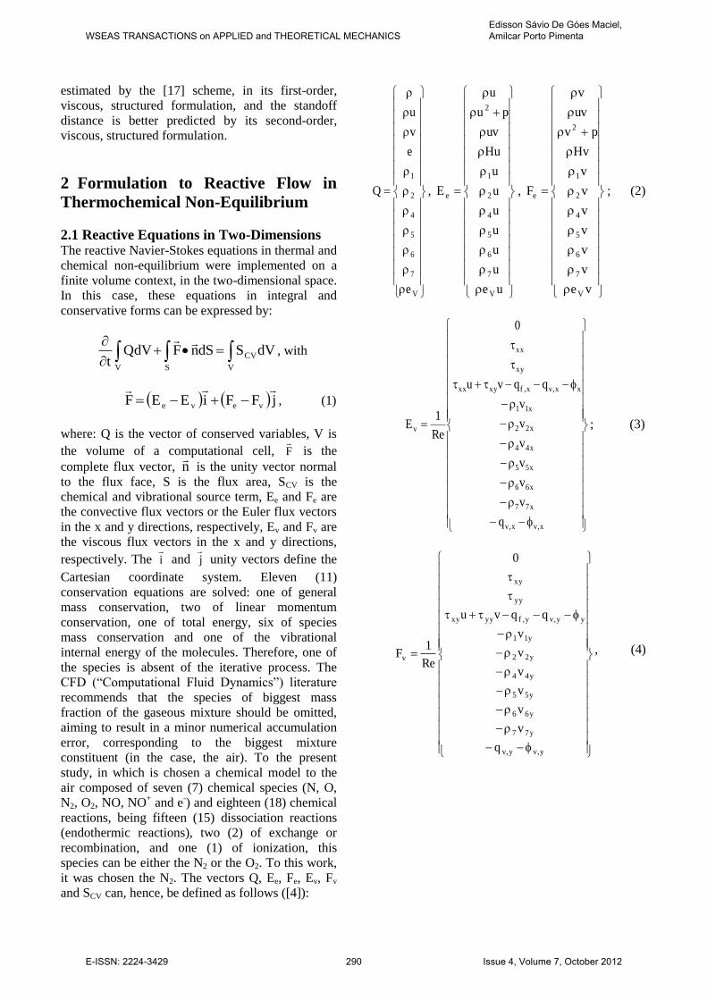
2.1 Reactive Equations in Two-Dimensions The reactive Navier-Stokes equations in thermal and
chemical non-equilibrium were implemented on a
finite volume context, in the two-dimensional space.
In this case, these equations in integral and
conservative forms can be expressed by:
V V
CV
S
dVSdSnFQdVt
, with
jFFiEEF veve
, (1)
where: Q is the vector of conserved variables, V is
the volume of a computational cell, F
is the
complete flux vector, n
is the unity vector normal
to the flux face, S is the flux area, SCV is the
chemical and vibrational source term, Ee and Fe are
the convective flux vectors or the Euler flux vectors
in the x and y directions, respectively, Ev and Fv are
the viscous flux vectors in the x and y directions,
respectively. The i
and j
unity vectors define the
Cartesian coordinate system. Eleven (11)
conservation equations are solved: one of general
mass conservation, two of linear momentum
conservation, one of total energy, six of species
mass conservation and one of the vibrational
internal energy of the molecules. Therefore, one of
the species is absent of the iterative process. The
CFD (“Computational Fluid Dynamics”) literature
recommends that the species of biggest mass
fraction of the gaseous mixture should be omitted,
aiming to result in a minor numerical accumulation
error, corresponding to the biggest mixture
constituent (in the case, the air). To the present
study, in which is chosen a chemical model to the
air composed of seven (7) chemical species (N, O,
N2, O2, NO, NO+ and e
-) and eighteen (18) chemical
reactions, being fifteen (15) dissociation reactions
(endothermic reactions), two (2) of exchange or
recombination, and one (1) of ionization, this
species can be either the N2 or the O2. To this work,
it was chosen the N2. The vectors Q, Ee, Fe, Ev, Fv
and SCV can, hence, be defined as follows ([4]):
V
7
6
5
4
2
1
e
e
v
u
Q ,
ue
u
u
u
u
u
u
Hu
uv
pu
u
E
V
7
6
5
4
2
1
2
e ,
ve
v
v
v
v
v
v
Hv
pv
uv
v
F
V
7
6
5
4
2
1
2
e ; (2)
x,vx,v
x77
x66
x55
x44
x22
x11
xx,vx,fxyxx
xy
xx
v
q
v
v
v
v
v
v
qqvu
0
Re
1E ; (3)
y,vy,v
y77
y66
y55
y44
y22
y11
yy,vy,fyyxy
yy
xy
v
q
v
v
v
v
v
v
qqvu
0
Re
1F , (4)
WSEAS TRANSACTIONS on APPLIED and THEORETICAL MECHANICSEdisson Sávio De Góes Maciel, Amilcar Porto Pimenta
E-ISSN: 2224-3429 290 Issue 4, Volume 7, October 2012
Page 4
mols
s,vs
mols
ss,v*
s,vs
7
6
5
4
2
1
CV
eee
0
0
0
0
S
, (5)
in which: is the mixture density; u and v are
Cartesian components of the velocity vector in the x
and y directions, respectively; p is the fluid static
pressure; e is the fluid total energy; 1, 2, 4, 5, 6,
7 are densities of the N, O, O2, NO, NO+ and e
-,
respectively; H is the mixture total enthalpy; eV is
the sum of the vibrational energy of the molecules;
the ’s are the components of the viscous stress
tensor; qf,x and qf,y are the frozen components of the
Fourier-heat-flux vector in the x and y directions,
respectively; qv,x and qv,y are the components of the
Fourier-heat-flux vector calculated with the
vibrational thermal conductivity and vibrational
temperature; svsx and svsy represent the species
diffusion flux, defined by the Fick law; x and y are
the terms of mixture diffusion; v,x and v,y are the
terms of molecular diffusion calculated at the
vibrational temperature; s is the chemical source
term of each species equation, defined by the law of
mass action; *ve is the molecular-vibrational-internal
energy calculated with the translational/rotational
temperature; and s is the translational-vibrational
characteristic relaxation time of each molecule.
The viscous stresses, in N/m2, are determined,
according to a Newtonian fluid model, by:
y
v
x
u
3
2
x
u2xx ,
x
v
y
uxy and
y
v
x
u
3
2
y
v2yy ,
(6)
in which is the fluid molecular viscosity.
The frozen components of the Fourier-heat-flux
vector, which considers only thermal conduction,
are defined by:
x
Tkq fx,f
and
y
Tkq fy,f
, (7)
where kf is the mixture frozen thermal conductivity,
calculated conform presented in subsection 2.3.4.
The vibrational components of the Fourier-heat-flux
vector are calculated as follows:
x
Tkq v
vx,v
and
y
Tkq v
vy,v
, (8)
in which kv is the vibrational thermal conductivity
and Tv is the vibrational temperature, what
characterizes this model as of two temperatures:
translational/rotational and vibrational. The
calculation of Tv and kv are demonstrated in
subsections 2.2.2 and 2.3.4, respectively.
The terms of species diffusion, defined by the
Fick law, to a condition of thermal non-equilibrium,
are determined by ([4]):
x
YDv
s,MF
ssxs
and
y
YDv
s,MF
ssys
,
(9)
with “s” referent to a given species, YMF,s being the
molar fraction of the species, defined as:
ns
1k
kk
ss
s,MF
M
MY (10)
and Ds is the species-effective-diffusion coefficient.
The diffusion terms x and y which appear in
the energy equation are defined by ([20]):
ns
1s
ssxsx hv and
ns
1s
ssysy hv , (11)
being hs the specific enthalpy (sensible) of the
chemical species “s”. Details of the calculation of
the specific enthalpy, see [21-22]. The molecular
diffusion terms calculated at the vibrational
temperature, v,x and v,y, which appear in the
vibrational-internal-energy equation are defined by
([4]):
WSEAS TRANSACTIONS on APPLIED and THEORETICAL MECHANICSEdisson Sávio De Góes Maciel, Amilcar Porto Pimenta
E-ISSN: 2224-3429 291 Issue 4, Volume 7, October 2012
Page 5
mols
s,vsxsx,v hv and
mols
s,vsysy,v hv , (12)
with hv,s being the specific enthalpy (sensible) of the
chemical species “s” calculated at the vibrational
temperature Tv. The sum of Eq. (12), as also those
present in Eq. (5), considers only the molecules of
the system, namely: N2, O2, NO, and NO+.
2.2 Thermodynamic Model/Thermodynamic
Properties
2.2.1 Definition of general parameters
ns
1s
ss
ns
1s
ss
ns
1s
ss McMRTMRTp
ns
1s
ss Mc , (13)
in which: is the mixture number in kg-mol/kg and
cs is the mass fraction (non-dimensional), defined by
ssc .
sss
ns
1s
s Mc
;
ns
1s
ssmixtmixt Mc1M1M ;
)TT(ee vs,v
*
s,v , (14)
with: s being the number of kg-mol/kg of species
“s” and Mmixt is the mixture molecular mass, in
kg/kg-mol.
2.2.2 Thermodynamic model
(a) Mixture translational internal energy:
s
ns
1s
0T
0s,T,v
ns
1s
ss,TT h'dT)'T(Cee
,
(15)
where: eT,s is the translational internal energy per
kg-mol of species “s”, in J/kg-mol. The specific heat
at constant volume per kg-mol of species “s” due to
translation, in J/(kg-mol.K), is defined by:
R5.1)T(C s,T,v . (16)
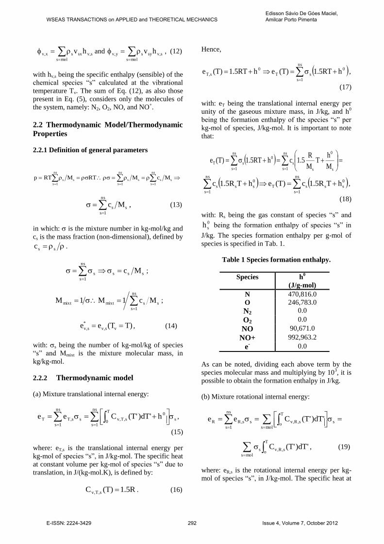
Hence,
ns
1s
0
sT
0
s,T hRT5.1)T(ehRT5.1)T(e ,
(17)
with: eT being the translational internal energy per
unity of the gaseous mixture mass, in J/kg, and h0
being the formation enthalpy of the species “s” per
kg-mol of species, J/kg-mol. It is important to note
that:
ns
1s s
0
s
s
ns
1s
0
sTM
hT
M
R5.1chRT5.1)T(e
ns
1s
0
sssT
ns
1s
0
sss hTR5.1c)T(ehTR5.1c ,
(18)
with: Rs being the gas constant of species “s” and 0
sh being the formation enthalpy of species “s” in
J/kg. The species formation enthalpy per g-mol of
species is specified in Tab. 1.
Table 1 Species formation enthalpy.
Species h0
(J/g-mol)
N 470,816.0
O 246,783.0
N2 0.0
O2 0.0
NO 90,671.0
NO+ 992,963.2
e- 0.0
As can be noted, dividing each above term by the
species molecular mass and multiplying by 103, it is
possible to obtain the formation enthalpy in J/kg.
(b) Mixture rotational internal energy:
mols
s
T
os,R,v
ns
1s
ss,RR 'dT)'T(Cee
mols
T
os,R,vs 'dT)'T(C , (19)
where: eR,s is the rotational internal energy per kg-
mol of species “s”, in J/kg-mol. The specific heat at
WSEAS TRANSACTIONS on APPLIED and THEORETICAL MECHANICSEdisson Sávio De Góes Maciel, Amilcar Porto Pimenta
E-ISSN: 2224-3429 292 Issue 4, Volume 7, October 2012
Page 6
constant volume per kg-mol of species “s” due to
rotation, in J/(kg-mol.K), is defined by:
mols
sRs,Rs,R,v RT)T(eRT)T(eRC
or
mols
ssR TRc)T(e , (20)
with eR being the rotational internal energy per unity
of gaseous mixture mass, in J/kg.
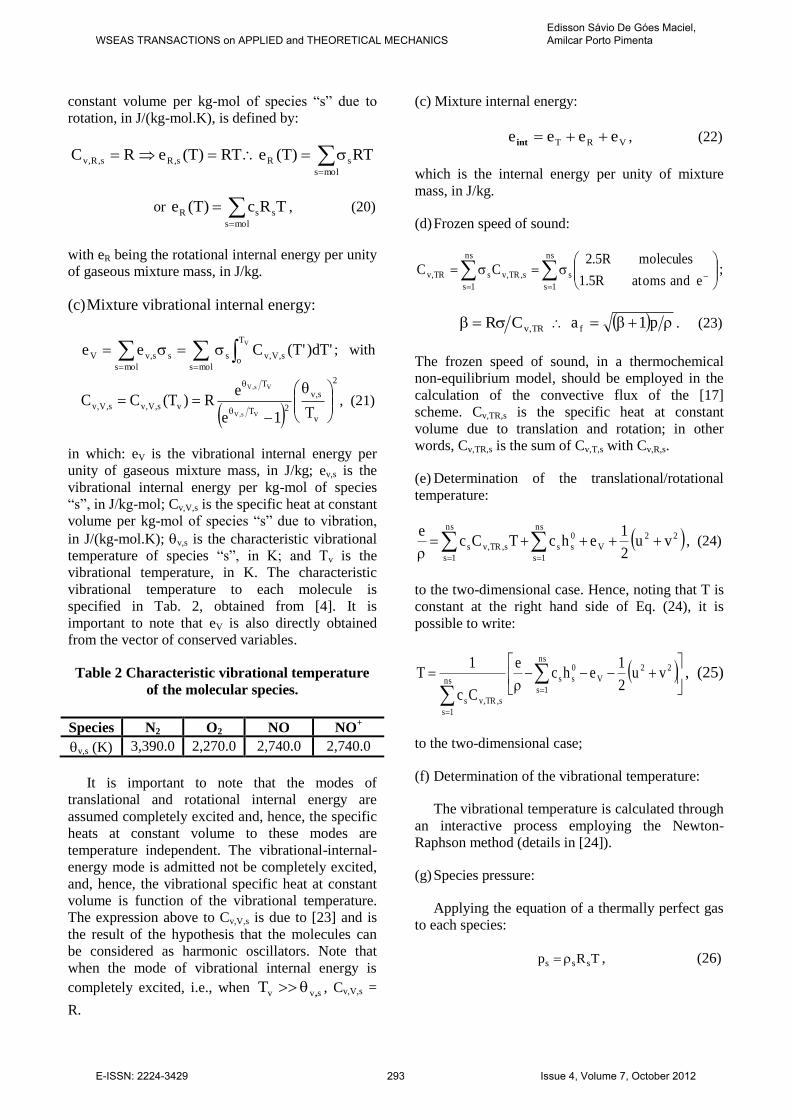
(c) Mixture vibrational internal energy:
'dT)'T(Ceemols
T
os,V,vs
mols
ss,vV
V
; with
2
v
s,v
2T
T
vs,V,vs,V,vT1e
eR)T(CC
Vs,V
Vs,V
, (21)
in which: eV is the vibrational internal energy per
unity of gaseous mixture mass, in J/kg; ev,s is the
vibrational internal energy per kg-mol of species
“s”, in J/kg-mol; Cv,V,s is the specific heat at constant
volume per kg-mol of species “s” due to vibration,
in J/(kg-mol.K); v,s is the characteristic vibrational
temperature of species “s”, in K; and Tv is the
vibrational temperature, in K. The characteristic
vibrational temperature to each molecule is
specified in Tab. 2, obtained from [4]. It is
important to note that eV is also directly obtained
from the vector of conserved variables.
Table 2 Characteristic vibrational temperature
of the molecular species.
Species N2 O2 NO NO+
v,s (K) 3,390.0 2,270.0 2,740.0 2,740.0
It is important to note that the modes of
translational and rotational internal energy are
assumed completely excited and, hence, the specific
heats at constant volume to these modes are
temperature independent. The vibrational-internal-
energy mode is admitted not be completely excited,
and, hence, the vibrational specific heat at constant
volume is function of the vibrational temperature.
The expression above to Cv,V,s is due to [23] and is
the result of the hypothesis that the molecules can
be considered as harmonic oscillators. Note that
when the mode of vibrational internal energy is
completely excited, i.e., when svvT , , Cv,V,s =
R.
(c) Mixture internal energy:
VRT eeee int , (22)
which is the internal energy per unity of mixture
mass, in J/kg.
(d) Frozen speed of sound:
ns
1s
ns
1s
ss,TR,vsTR,veandatomsR5.1
moleculesR5.2CC ;
TR,vCR p1a f . (23)
The frozen speed of sound, in a thermochemical
non-equilibrium model, should be employed in the
calculation of the convective flux of the [17]
scheme. Cv,TR,s is the specific heat at constant
volume due to translation and rotation; in other
words, Cv,TR,s is the sum of Cv,T,s with Cv,R,s.
(e) Determination of the translational/rotational
temperature:
ns
1s
22ns
1s
V
0
sss,TR,vs vu2
1ehcTCc
e, (24)
to the two-dimensional case. Hence, noting that T is
constant at the right hand side of Eq. (24), it is
possible to write:
22ns
1s
V
0
ssns
1s
s,TR,vs
vu2
1ehc
e
Cc
1T , (25)
to the two-dimensional case;
(f) Determination of the vibrational temperature:
The vibrational temperature is calculated through
an interactive process employing the Newton-
Raphson method (details in [24]).
(g) Species pressure:
Applying the equation of a thermally perfect gas
to each species:
TRp sss , (26)
WSEAS TRANSACTIONS on APPLIED and THEORETICAL MECHANICSEdisson Sávio De Góes Maciel, Amilcar Porto Pimenta
E-ISSN: 2224-3429 293 Issue 4, Volume 7, October 2012
Page 7
where: ss c is the density of species “s”, Rs is
the gas constant to species “s” and T is the
translational/rotational temperature.
2.3 Transport Model/Transport Physical
Properties
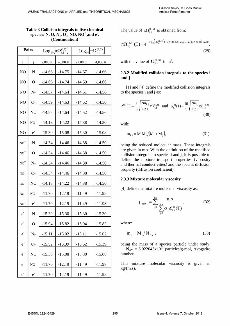
2.3.1 Collision integrals to species i and j
In Table 3 are presented values of )1,1(j,i10Log and
)2,2(j,i10Log to temperature values of 2,000 K and
4,000 K. The indexes i and j indicate, in the present
case, the collision partners; in other words, the pair
formed by one atom and one atom, one atom and
one molecule, etc. These data obtained from [1].
Table 3 Collision integrals to five chemical
species: N, O, N2, O2, NO, NO+ and e
-.
Pairs )1,1(
j,i10Log )2,2(
j,i10Log
i j 2,000 K 4,000 K 2,000 K 4,000 K
N N -14.08 -14.11 -14.74 -14.82
N O -14.76 -14.86 -14.69 -14.80
N N2 -14.67 -14.75 -14.59 -14.66
N O2 -14.66 -14.74 -14.59 -14.66
N NO -14.66 -14.75 -14.67 -14.66
N NO+ -14.34 -14.46 -14.38 -14.50
N e- -15.30 -15.30 -15.30 -15.30
The data aforementioned define a linear
interpolation to values of )k,k(j,i10Log as function
of Ln(T), with k = 1, 2, through the linear equation:
)K000,2T(Log)T(Log )k,k(
j,i10
)k,k(
j,i10
000,2TLnslope , (27)
in which:
)K000,4T(Logslope )k,k(
j,i10
2Ln)K000,2T(Log )k,k(
j,i10 .
(28)
Table 3 Collision integrals to five chemical
species: N, O, N2, O2, NO, NO+ and e
-.
(Continuation)
Pairs )1,1(
j,i10Log )2,2(
j,i10Log
i j 2,000 K 4,000 K 2,000 K 4,000 K
O N -14.76 -14.86 -14.69 -14.80
O O -14.11 -14.14 -14.71 -14.79
O N2 -14.63 -14.72 -14.55 -14.64
O O2 -14.69 -14.76 -14.62 -14.69
O NO -14.66 -14.74 -14.59 -14.66
O NO+ -14.34 -14.46 -14.38 -14.50
O e- -15.94 -15.82 -15.94 -15.82
N2 N -14.67 -14.75 -14.59 -14.66
N2 O -14.63 -14.72 -14.55 -14.64
N2 N2 -14.56 -14.65 -14.50 -14.58
N2 O2 -14.58 -14.63 -14.51 -14.54
N2 NO -14.57 -14.64 -14.51 -14.56
N2 NO+ -14.34 -14.46 -14.38 -14.50
N2 e- -15.11 -15.02 -15.11 -15.02
O2 N -14.66 -14.74 -14.59 -14.66
O2 O -14.69 -14.76 -14.62 -14.69
O2 N2 -14.58 -14.63 -14.51 -14.54
O2 O2 -14.60 -14.64 -14.54 -14.57
O2 NO -14.59 -14.63 -14.52 -14.56
O2 NO+ -14.34 -14.46 -14.38 -14.50
O2 e- -15.52 -15.39 -15.52 -15.39
WSEAS TRANSACTIONS on APPLIED and THEORETICAL MECHANICSEdisson Sávio De Góes Maciel, Amilcar Porto Pimenta
E-ISSN: 2224-3429 294 Issue 4, Volume 7, October 2012
Page 8
Table 3 Collision integrals to five chemical
species: N, O, N2, O2, NO, NO+ and e
-.
(Continuation)
Pairs )1,1(
j,i10Log )2,2(
j,i10Log
i j 2,000 K 4,000 K 2,000 K 4,000 K
NO N -14.66 -14.75 -14.67 -14.66
NO O -14.66 -14.74 -14.59 -14.66
NO N2 -14.57 -14.64 -14.51 -14.56
NO O2 -14.59 -14.63 -14.52 -14.56
NO NO -14.58 -14.64 -14.52 -14.56
NO NO+ -14.18 -14.22 -14.38 -14.50
NO e- -15.30 -15.08 -15.30 -15.08
NO+ N -14.34 -14.46 -14.38 -14.50
NO+ O -14.34 -14.46 -14.38 -14.50
NO+ N2 -14.34 -14.46 -14.38 -14.50
NO+ O2 -14.34 -14.46 -14.38 -14.50
NO+ NO -14.18 -14.22 -14.38 -14.50
NO+ NO
+ -11.70 -12.19 -11.49 -11.98
NO+ e
- -11.70 -12.19 -11.49 -11.98
e- N -15.30 -15.30 -15.30 -15.30
e- O -15.94 -15.82 -15.94 -15.82
e- N2 -15.11 -15.02 -15.11 -15.02
e- O2 -15.52 -15.39 -15.52 -15.39
e- NO -15.30 -15.08 -15.30 -15.08
e- NO
+ -11.70 -12.19 -11.49 -11.98
e- e
- -11.70 -12.19 -11.49 -11.98
The value of )k,k(j,i is obtained from:
10Ln000,2TLnslope)K000,2T(Log)k,k(
j,i
)k,k(j,i10e)T(
,
(29)
with the value of )k,k(
j,i in m2.
2.3.2 Modified collision integrals to the species i
and j
[1] and [4] define the modified collision integrals
to the species i and j as:
)1,1(j,i
j,i)1(j,i
RT
m2
3
8)T(
and )2,2(
j,i
j,i)2(j,i
RT
m2
5
16)T(
,
(30)
with:
jijij,i MMMMm , (31)
being the reduced molecular mass. These integrals
are given in m.s. With the definition of the modified
collision integrals to species i and j, it is possible to
define the mixture transport properties (viscosity
and thermal conductivities) and the species diffusion
property (diffusion coefficient).
2.3.3 Mixture molecular viscosity
[4] define the mixture molecular viscosity as:
ns
1ins
1j
)2(
j,ij
iimixt
)T(
m, (32)
where:
AVii NMm , (33)
being the mass of a species particle under study;
NAV = 6.022045x10²³
particles/g-mol, Avogadro
number.
This mixture molecular viscosity is given in
kg/(m.s).
WSEAS TRANSACTIONS on APPLIED and THEORETICAL MECHANICSEdisson Sávio De Góes Maciel, Amilcar Porto Pimenta
E-ISSN: 2224-3429 295 Issue 4, Volume 7, October 2012
Page 9
2.3.4 Vibrational, frozen, rotational and
translational thermal conductivities
All thermal conductivities are expressed in
J/(m.s.K). [4] defines the mixture vibrational,
rotational and translational thermal conductivities,
as also the species diffusion coefficient, as follows.
(a) Translational thermal conductivity:
The mode of translational internal energy is
admitted completely excited; hence, the thermal
conductivity of the translational internal energy is
determined by:
ns
1ins
1j
)2(
j,ijj,i
i
BoltzmannT
)T(a
k4
15k , (34)
in which:
kBoltzmann = Boltzmann constant = 1,380622x
10-23
J/K;
2ji
jiji
j,iMM1
MM54.245.0)MM1(1a
. (35)
(b) Rotational thermal conductivity:
The mode of rotational internal energy is also
considered fully excited; hence, the thermal
conductivity due to rotational internal energy is
defined by:
molins
1j
)1(
j,ij
i
BoltzmannR
)T(
kk . (36)
(c) Frozen thermal conductivity:
kf = kT+kR. (37)
(d) Thermal conductivity due to molecular vibration:
The mode of vibrational internal energy,
however, is assumed be partially excited; hence, the
vibrational thermal conductivity is calculated
according to [3] by:
molins
1j
)1(
j,ij
ii,V,v
BoltzmannV
)T(
RCkk , (38)
with Cv,V,i obtained from Eq. (21).
2.3.5 Species diffusion coefficient
The mass-diffusion-effective coefficient, Di, of
the species “i” in the gaseous mixture is defined by:
ns
1j
j,ij
iii
2
i
D
M1MD and
)T(p
TkD
)1(
j,i
Boltzmann
j,i
, (39)
where: Di,j is the binary diffusion coefficient to a
pair of particles of the species “i” and “j” and is
related with the modified collision integral conform
described above, in Eq. (39). This coefficient is
measured in m2/s.
2.4 Chemical Model The chemical model employed to this case of
thermochemical non-equilibrium is the seven
species model of [46], using the N, O, N2, O2, NO,
NO+ and e
- species. This formulation uses, in the
calculation of the species production rates, a
temperature of reaction rate control, introduced in
the place of the translational/rotational temperature,
which is employed in the calculation of such rates.
This procedure aims a couple between vibration and
dissociation. This temperature is defined as:
vrrc TTT , where T is the
translational/rotational temperature and Tv is the
vibrational temperature. This temperature Trrc
replaces the translational/rotational temperature in
the calculation of the species production rates,
according to [25].
2.4.1 Law of Mass Action
The symbolic representation of a given reaction in
the present work follows the [26] formulation and is
represented by:
ns
1s
ssr
ns
1s
ssr AA ''' , r = 1,..., nr. (40)
The law of mass action applied to this system of
chemical reactions is defined by:
WSEAS TRANSACTIONS on APPLIED and THEORETICAL MECHANICSEdisson Sávio De Góes Maciel, Amilcar Porto Pimenta
E-ISSN: 2224-3429 296 Issue 4, Volume 7, October 2012
Page 10
nr
1r
ns
1s s
s
br
ns
1s s
s
frsrsrss
srsr
Mk
MkM
'''
''' ,
(41)
where As represents the chemical symbol of species
“s”, “ns” is the number of species of the present
study (reactants and products) involved in the
considered reaction; “nr” is the number of reactions
considered in the chemical model; '
sr e ''
sr are the
stoichiometric coefficients to reactants and products,
respectively; TCB
fr eATk / and E
br DTk ,
with A, B, C, D and E being constants of a specific
chemical reaction under study [“fr” = forward
reaction and “br” = backward reaction]. It is
important to note that erfrbr kkk , with ker being
the equilibrium constant which depends only of the
thermodynamic quantities. In this work, ns = 7 and
nr = 18. Table 4 presents the values to A, B, C, D
and E for the forward reaction rates of the 18
chemical reactions. Table 5 presents the values to A,
B, C, D and E for the backward reaction rates. The
eighth equation takes into account the formation of
an electron from the ionization of the NO. For this
case, the backward reaction rate depends only of the
vibrational temperature.
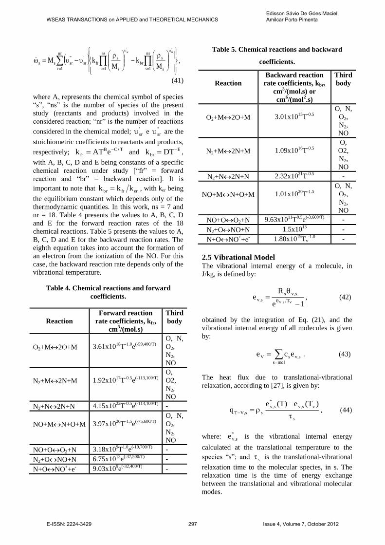
Table 4. Chemical reactions and forward
coefficients.
Reaction
Forward reaction
rate coefficients, kfr,
cm3/(mol.s)
Third
body
O2+M2O+M
3.61x10¹⁸
T-1.0
e(-59,400/T)
O, N,
O2,
N2,
NO
N2+M2N+M
1.92x10¹⁷
T-0.5
e(-113,100/T)
O,
O2,
N2,
NO
N2+N2N+N 4.15x10²²
T-0.5
e(-113,100/T)
-
NO+MN+O+M
3.97x10²⁰
T-1.5
e(-75,600/T)
O, N,
O2,
N2,
NO
NO+OO2+N 3.18x10⁹T
1.0e
(-19,700/T) -
N2+ONO+N 6.75x10¹³
e(-37,500/T)
-
N+ONO++e
- 9.03x10
9e
(-32,400/T) -
Table 5. Chemical reactions and backward
coefficients.
Reaction
Backward reaction
rate coefficients, kbr,
cm3/(mol.s) or
cm6/(mol
2.s)
Third
body
O2+M2O+M
3.01x10¹⁵
T-0.5
O, N,
O2,
N2,
NO
N2+M2N+M
1.09x10¹⁶
T-0.5
O,
O2,
N2,
NO
N2+N2N+N 2.32x10²¹
T-0.5
-
NO+MN+O+M
1.01x10²⁰
T-1.5
O, N,
O2,
N2,
NO
NO+OO2+N 9.63x10¹¹
T0.5
e(-3,600/T)
-
N2+ONO+N 1.5x10¹³
-
N+ONO++e
- 1.80x10
19Tv
-1.0 -
2.5 Vibrational Model The vibrational internal energy of a molecule, in
J/kg, is defined by:
1e
Re
Vs,V T
s,vs
s,v
, (42)
obtained by the integration of Eq. (21), and the
vibrational internal energy of all molecules is given
by:
mols
s,vsV ece . (43)
The heat flux due to translational-vibrational
relaxation, according to [27], is given by:
s
vs,v
*
s,v
ss,VT
)T(e)T(eq
, (44)
where: *
s,ve is the vibrational internal energy
calculated at the translational temperature to the
species “s”; and s is the translational-vibrational
relaxation time to the molecular species, in s. The
relaxation time is the time of energy exchange
between the translational and vibrational molecular
modes.
WSEAS TRANSACTIONS on APPLIED and THEORETICAL MECHANICSEdisson Sávio De Góes Maciel, Amilcar Porto Pimenta
E-ISSN: 2224-3429 297 Issue 4, Volume 7, October 2012
Page 11
2.5.1 Vibrational characteristic time of [28]
According to [28], the relaxation time of molar
average of [29] is described by:
ns
1l
WM
l,sl
ns
1l
l
WM
ss , (45)
with:
WM
l,s
is the relaxation time between species of
[29];
WM
s
is the vibrational characteristic time of
[29];
lAVll mNc and AVll NMm .
(46)
2.5.2 Definition of WM
l,s
:
For temperatures inferior to or equal to 8,000 K,
[29] give the following semi-empirical correlation to
the vibrational relaxation time due to inelastic
collisions:
42.18015.0TA
l
WM
l,s
41l,s
31l,se
p
B
, (47)
where:
B = 1.013x10⁵Ns/m
2 ([30]);
pl is the partial pressure of species “l” in N/m2;
34
s,v
21
l,s
3
l,s 10x16.1A ([30]); (48)
ls
ls
l,sMM
MM
, (49)
being the reduced molecular mass of the collision
partners: kg/kg-mol;
T and s,v in Kelvin.
2.5.3 [25] correction time
For temperatures superiors to 8,000 K, the Eq. (43)
gives relaxation times less than those observed in
experiments. To temperatures above 8,000 K, [25]
suggests the following relation to the vibrational
relaxation time:
svs
P
sn
1
, (50)
where:
TR8 s
s , (51)
being the molecular average velocity in m/s;
2
20
vT
000,5010
, (52)
being the effective collision cross-section to
vibrational relaxation in m2; and
sss mn , (53)
being the density of the number of collision particles
of species “s”. s in kg/m3 and ms in kg/particle,
defined by Eq. (33).
Combining the two relations, the following
expression to the vibrational relaxation time is
obtained:
P
s
WM
ss . (54)
[25] emphasizes that this expression [Eq. (54)] to
the vibrational relaxation time is applicable to a
range of temperatures much more vast.
3 Structured [17] Algorithm to
Thermochemical Non-Equilibrium Considering the two-dimensional and structured
case, the algorithm follows that described in [21],
considering, however, the vibrational contribution
([31]) and the version of the two-temperature model
to the frozen speed of sound [Eq. (23)]. Hence, the
discrete-dynamic-convective flux is defined by:
RL
j,2/1ij,2/1ij,2/1i
aH
av
au
a
aH
av
au
a
M2
1SR
(55a)
WSEAS TRANSACTIONS on APPLIED and THEORETICAL MECHANICSEdisson Sávio De Góes Maciel, Amilcar Porto Pimenta
E-ISSN: 2224-3429 298 Issue 4, Volume 7, October 2012
Page 12
j,2/1i
y
x
LR
j,2/1i
0
pS
pS
0
aH
av
au
a
aH
av
au
a
2
1
,
(55b)
the discrete-chemical-convective flux is defined by:
R7
6
5
4
2
1
L7
6
5
4
2
1
j,2/1ij,2/1ij,2/1i
a
a
a
a
a
a
a
a
a
a
a
a
M2
1SR
L7
6
5
4
2
1
R7
6
5
4
2
1
j,2/1i
a
a
a
a
a
a
a
a
a
a
a
a
2
1, (56)
and the discrete-vibrational-convective flux is
determined by:
RvLvj,2/1ij,2/1ij,2/1i aeaeM2
1SR
LvRvj,2/1i aeae
2
1 . (57)
The same definitions presented in [21-22] are valid
to this algorithm. The time integration is performed
employing the Runge-Kutta explicit method of five
stages, second-order accurate, to the three types of
convective flux. To the dynamic part, this method
can be represented in general form by:
)k(
j,i
)1n(
j,i
j,i
)1k(
j,ij,ik
)0(
j,i
)k(
j,i
)n(
j,i
)0(
j,i
QQ
VQRtQQ
QQ
, (58)
to the chemical part, it can be represented in general
form by:
)k(
j,i
)1n(
j,i
)1k(
j,iCj,i
)1k(
j,ij,ik
)0(
j,i
)k(
j,i
)n(
j,i
)0(
j,i
QQ
QSVQRtQQ
QQ
,
(59)
where the chemical source term SC is calculated
with the temperature Trrc. Finally, to the vibrational
part:
)k(
j,i)1n(
j,i
)1k(j,ivj,i
)1k(j,ij,ik
)0(j,i
)k(j,i
)n(j,i
)0(j,i
QQ
QSVQRtQQ
QQ
, (60)
in which:
mols
s,vs,C
mols
s,VTv eSqS ; (61)
k = 1,...,5; 1 = 1/4, 2 = 1/6, 3 = 3/8, 4 = 1/2 and
5 = 1. This scheme is first-order accurate in space
and second-order accurate in time. The second-order
of spatial accuracy is obtained by the “MUSCL”
procedure (details in [32]).
The [17] scheme in its first-order two-
dimensional unstructured version to an ideal gas
formulation is presented in [33]. The extension to
reactive flow in thermochemical non-equilibrium
can be deduced from the present code.
The viscous formulation follows that of [34],
which adopts the Green theorem to calculate
primitive variable gradients. The viscous vectors are
obtained by arithmetical average between cell (i,j)
and its neighbours. As was done with the convective
terms, there is a need to separate the viscous flux in
three parts: dynamical viscous flux, chemical
viscous flux and vibrational viscous flux. The
dynamical part corresponds to the first four
equations of the Navier-Stokes ones, the chemical
part corresponds to the following six equations and
the vibrational part corresponds to the last equation.
The spatially variable time step technique has
provided excellent convergence gains as
demonstrated in [18-19] and is implemented in the
code presented in this work. Details in [18-19; 22].
4 Results
Tests were performed in one personal computer
Notebook with Dual Core Intel Pentium processor
of 2.30 GHz of “clock” and 2.0 GBytes of RAM. As
the interest of this work is steady state problems, it
WSEAS TRANSACTIONS on APPLIED and THEORETICAL MECHANICSEdisson Sávio De Góes Maciel, Amilcar Porto Pimenta
E-ISSN: 2224-3429 299 Issue 4, Volume 7, October 2012
Page 13
is necessary to define a criterion which guarantees
the convergence of the numerical results. The
criterion adopted was to consider a reduction of no
minimal four (4) orders of magnitude in the value of
the maximum residual in the calculation domain, a
typical CFD-community criterion. The residual of
each cell was defined as the numerical value
obtained from the discretized conservation
equations. As there are eleven (11) conservation
equations to each cell, the maximum value obtained
from these equations is defined as the residual of
this cell. Hence, this residual is compared with the
residual of the other cells, calculated of the same
way, to define the maximum residual in the
calculation domain. In the simulations, the attack
angle was set equal to zero.
4.1 Initial and Boundary Conditions to the
Studied Problem The initial conditions are presented in Tab. 6. The
Reynolds number is obtained from data of [35]. The
boundary conditions to this problem of reactive flow
are detailed in [24], as well the geometry in study,
the meshes employed in the simulations and the
description of the computational configuration.
Table 6 Initial conditions to the problem of the
blunt body.
Property Value
M 8.78
0.00326 kg/m3
p 687 Pa
U 4,776 m/s
T 694 K
Tv, 694 K
altitude 40,000 m
cN 10-9
cO 0.07955
2Oc 0.13400
cNO 0.05090
cNO+ 0.0
ce- 0.0
L 2.0 m
Re 2.3885x10⁶
The geometry is a blunt body with 1.0 m of nose
ratio and parallel rectilinear walls. The far field is
located at 20.0 times the nose ratio in relation to the
configuration nose. The dimensionless employed in
the Euler and Navier-Stokes equations in this study
are also described in [24].
4.2 Studied Cases
Table 7 presents the studied cases in this work, the
mesh characteristics and the order of accuracy of the
[17] scheme.
Table 7 Studied cases, mesh characteristics and
accuracy order.
Case Mesh Accuracy
Order
Inviscid – 2D 63x60 Firsta
Viscous – 2D 63x60 (7.5%)c First
a
Inviscid – 2D 63x60 Seconda
Viscous – 2D 63x60 (7.5%) Seconda
Inviscid – 2D 63x60 Firstb
Viscous – 2D 63x60 (7.5%) Firstb
a Structured spatial discretization; b Unstructured spatial discretization; c
Exponential stretching..
4.3 Results in Thermochemical Non-
Equilibrium
4.3.1 Inviscid, structured and first-order
accurate case
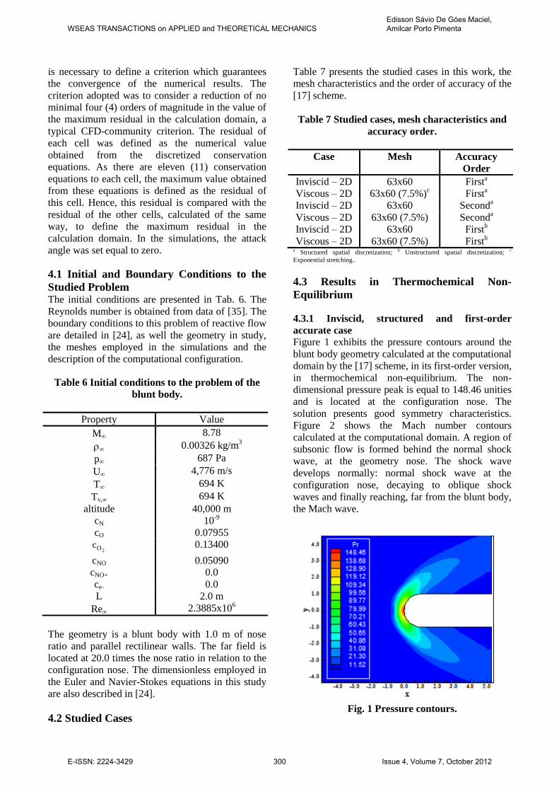
Figure 1 exhibits the pressure contours around the
blunt body geometry calculated at the computational
domain by the [17] scheme, in its first-order version,
in thermochemical non-equilibrium. The non-
dimensional pressure peak is equal to 148.46 unities
and is located at the configuration nose. The
solution presents good symmetry characteristics.
Figure 2 shows the Mach number contours
calculated at the computational domain. A region of
subsonic flow is formed behind the normal shock
wave, at the geometry nose. The shock wave
develops normally: normal shock wave at the
configuration nose, decaying to oblique shock
waves and finally reaching, far from the blunt body,
the Mach wave.
Fig. 1 Pressure contours.
WSEAS TRANSACTIONS on APPLIED and THEORETICAL MECHANICSEdisson Sávio De Góes Maciel, Amilcar Porto Pimenta
E-ISSN: 2224-3429 300 Issue 4, Volume 7, October 2012
Page 14
Fig. 2 Mach number contours.
Figure 3 presents the contours of the
translational/rotational temperature distribution
calculated at the computational domain. The
translational/rotational temperature reaches a peak
of 8,102 K at the configuration nose and determines
an appropriated region to dissociation of N2 and O2.
Along the blunt body, the translational/rotational
temperature assumes an approximated value of
6,000 K, what also represents a good value to the
dissociation firstly of O2 and, in second place, of the
N2.
Fig. 3 T/R temperature contours.
Figure 4 exhibits the contours of the vibrational
temperature calculated at the two-dimensional
computational domain. Its peak reaches a value of
5,415 K and also contributes to the dissociation of
N2 and O2, since the employed temperature to the
calculation of the forward and backward reaction
rates (reaction-rate-control temperature, Trrc) in the
thermochemical non-equilibrium is equal to
VT.T , the square root of the product between the
translational/rotational temperature and the
vibrational temperature. Hence, the effective
temperature to the calculation of the chemical
phenomena guarantees the couple between the
vibrational mode and the dissociation reactions. In
this configuration nose region, the temperature Trrc
reaches, in the steady state condition, the
approximated value of 6,624 K, assuring that the
dissociation phenomena described above occurs.
Good symmetry characteristics are observed.
Fig. 4 Vibrational temperature contours.
Fig. 5 Mass fraction distribution at the blunt
body stagnation line.
Figure 5 shows the mass fraction distribution of
the seven chemical species under study, namely: N,
O, N2, O2, NO, NO+ and e
-, along the geometry
stagnation line or geometry symmetry line. As can
be observed from this figure, enough dissociation of
N2 and O2 occur, with the consequent meaningful
increase of N and of NO in the gaseous mixture. As
WSEAS TRANSACTIONS on APPLIED and THEORETICAL MECHANICSEdisson Sávio De Góes Maciel, Amilcar Porto Pimenta
E-ISSN: 2224-3429 301 Issue 4, Volume 7, October 2012
Page 15
mentioned early, this behaviour is expected due to
the effective peak temperature reached at the
calculation domain. The NO presented the biggest
absolute increase in its formation, whereas the N
presented the biggest relative increase. The O has
not a meaningful increase due to the formation of
the NO+. The formation of e
- is also discrete.
4.3.2 Viscous, structured and first-order
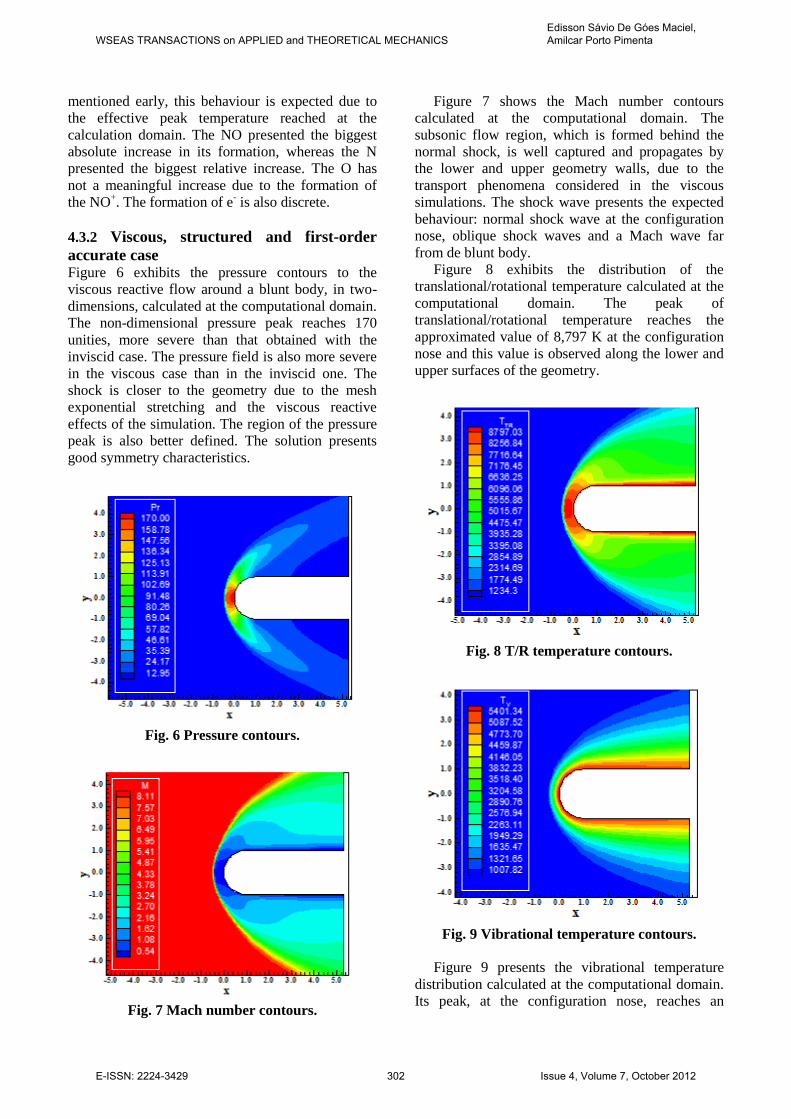
accurate case Figure 6 exhibits the pressure contours to the
viscous reactive flow around a blunt body, in two-
dimensions, calculated at the computational domain.
The non-dimensional pressure peak reaches 170
unities, more severe than that obtained with the
inviscid case. The pressure field is also more severe
in the viscous case than in the inviscid one. The
shock is closer to the geometry due to the mesh
exponential stretching and the viscous reactive
effects of the simulation. The region of the pressure
peak is also better defined. The solution presents
good symmetry characteristics.
Fig. 6 Pressure contours.
Fig. 7 Mach number contours.
Figure 7 shows the Mach number contours
calculated at the computational domain. The
subsonic flow region, which is formed behind the
normal shock, is well captured and propagates by
the lower and upper geometry walls, due to the
transport phenomena considered in the viscous
simulations. The shock wave presents the expected
behaviour: normal shock wave at the configuration
nose, oblique shock waves and a Mach wave far
from de blunt body.
Figure 8 exhibits the distribution of the
translational/rotational temperature calculated at the
computational domain. The peak of
translational/rotational temperature reaches the
approximated value of 8,797 K at the configuration
nose and this value is observed along the lower and
upper surfaces of the geometry.
Fig. 8 T/R temperature contours.
Fig. 9 Vibrational temperature contours.
Figure 9 presents the vibrational temperature
distribution calculated at the computational domain.
Its peak, at the configuration nose, reaches an
WSEAS TRANSACTIONS on APPLIED and THEORETICAL MECHANICSEdisson Sávio De Góes Maciel, Amilcar Porto Pimenta
E-ISSN: 2224-3429 302 Issue 4, Volume 7, October 2012
Page 16
approximated value of 5,401 K. The effective
temperature to the calculation of the dissociation
and recombination reactions, Trrc, is equal
approximately to 6,893 K, which guarantees that
processes of dissociation of O2 and N2 can be
captured by the employed formulation. This value of
effective temperature to the viscous reactive
simulations is superior to that obtained in the
inviscid case. Good symmetry characteristics are
observed in these figures.
Figure 10 exhibits the mass fraction distribution
of the seven chemical species under study along the
geometry stagnation line. As can be observed,
enough dissociation of the N2 and O2 occurs, with
the consequent meaningful increase of the N and of
the NO, with reduction of the mass fraction of the
O, in the gaseous mixture. The behaviour of the N
and of the NO is expected due to the temperature
peak reached in the calculation domain. The O
reduction is also expected due to the formation of
the NO+. The biggest absolute increase in the
formation of a species was due to the NO, while, in
relative terms, was due to the N. As can also be
noted, the mass fraction of the NO tends to assume a
constant value at the configuration nose. This is due
to the same behaviour observed in the mass fraction
distributions of the N and O, close to the
configuration nose (constancy).
Fig. 10 Mass fraction distribution at the blunt
body stagnation line.
4.3.3 Inviscid, structured and second-order
accurate case
Figure 11 shows the pressure contours obtained by
the inviscid simulation performed by the second-
order [17] scheme employing a minmod non-linear
flux limiter. The non-dimensional pressure peak is
approximately equal to 145 unities, slightly inferior
to the respective peak obtained by the first-order
solution. This pressure peak occurs at the
configuration nose. The solution presents good
symmetry characteristics. Figure 12 presents the
Mach number contours obtained at the
computational domain. The subsonic region which
is formed behind the normal shock wave is well
characterized at the configuration nose.
Fig. 11 Pressure contours.
Good symmetry characteristics are observed. The
shock wave presents the expected behaviour,
passing from a normal shock at the configuration
stagnation line to a Mach wave far from the blunt
body.
Fig. 12 Mach number contours.
Figure 13 exhibits the contours of the
translational/rotational temperature distribution
calculated at the computational domain. The
translational/rotational temperature peak occurs at
the configuration nose and is approximately equal to
8,218 K. Figure 14 presents the contours of the
vibrational temperature distribution calculated at the
WSEAS TRANSACTIONS on APPLIED and THEORETICAL MECHANICSEdisson Sávio De Góes Maciel, Amilcar Porto Pimenta
E-ISSN: 2224-3429 303 Issue 4, Volume 7, October 2012
Page 17
computational domain. The vibrational temperature
peak is approximately equal to 3,139 K and is
observed at the configuration nose. The effective
temperature to calculation of the reaction rates
(reaction rate control temperature, Trrc) is
approximately equal to 5,079 K, which represents a
temperature capable to capture the dissociation
phenomena of N2 and O2. Good symmetry
characteristics are observed in both figures.
Fig. 13 T/R temperature contours.
Fig. 14 Vibrational temperature contours.
Figure 15 exhibits the mass fraction distribution
of the seven chemical species under study, namely:
N, O, N2, O2, NO, NO+ and e
-, along the geometry
stagnation line. As can be observed, discrete
dissociation of N2 and O2 occur, with consequent
discrete increase of the N and of the NO, with
subsequent reduction of the O, in the gaseous
mixture. This behaviour is expected due to the
effective temperature peak reached at the
computational domain to the calculation of
thermochemical non-equilibrium and to a second-
order numerical formulation, which behaves in a
more conservative way (see [22]), providing minor
dissociation of N2 and O2.
Fig. 15 Mass fraction distribution at the blunt
body stagnation line.
4.3.4 Viscous, structured and second-order
accurate case
Figure 16 exhibits the pressure contours calculated
at the computational domain to the studied
configuration of blunt body. The non-dimensional
pressure peak is approximately equal to 164 unities,
less than the respective value obtained by the first-
order solution. The shock is positioned closer to the
blunt body due to the mesh stretching and the
employed-viscous-reactive formulation. Good
symmetry characteristics are observed.
Fig. 16 Pressure contours.
Figure 17 shows the Mach number contours
obtained at the computational domain. The subsonic
region behind the normal shock wave, at the
stagnation line, is well captured by the solution.
WSEAS TRANSACTIONS on APPLIED and THEORETICAL MECHANICSEdisson Sávio De Góes Maciel, Amilcar Porto Pimenta
E-ISSN: 2224-3429 304 Issue 4, Volume 7, October 2012
Page 18
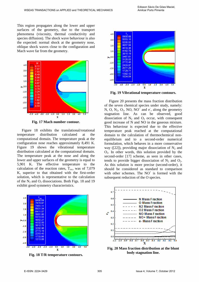
This region propagates along the lower and upper
surfaces of the geometry, due to the transport
phenomena (viscosity, thermal conductivity and
species diffusion). The shock wave behaviour is also
the expected: normal shock at the geometry nose,
oblique shock waves close to the configuration and
Mach wave far from the geometry.
Fig. 17 Mach number contour.
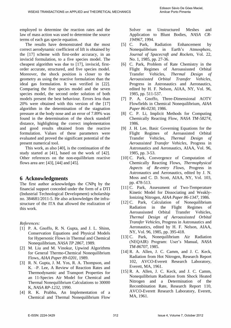
Figure 18 exhibits the translational/rotational
temperature distribution calculated at the
computational domain. The temperature peak at the
configuration nose reaches approximately 8,491 K.
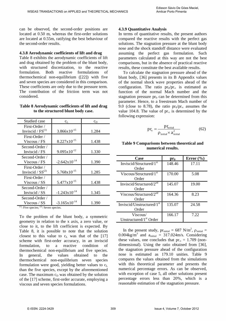
Figure 19 shows the vibrational temperature
distribution calculated at the computational domain.
The temperature peak at the nose and along the
lower and upper surfaces of the geometry is equal to
5,901 K. The effective temperature to the
calculation of the reaction rates, Trrc, was of 7,079
K, superior to that obtained with the first-order
solution, which is representative to the calculation
of the N2 and O2 dissociations. Both Figs. 18 and 19
exhibit good symmetry characteristics.
Fig. 18 T/R temperature contours.
Fig. 19 Vibrational temperature contours.
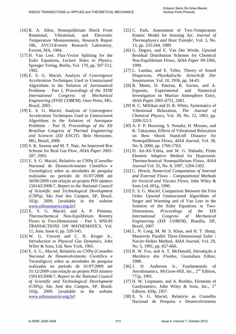
Figure 20 presents the mass fraction distribution
of the seven chemical species under study, namely:
N, O, N2, O2, NO, NO+ and e
-, along the geometry
stagnation line. As can be observed, good
dissociation of N2 and O2 occur, with consequent
good increase of N and NO in the gaseous mixture.
This behaviour is expected due to the effective
temperature peak reached at the computational
domain to the calculation of thermochemical non-
equilibrium and to a second-order numerical
formulation, which behaves in a more conservative
way ([22]), providing major dissociation of N2 and
O2. In other words, this solution provided by the
second-order [17] scheme, as seen in other cases,
tends to provide bigger dissociation of N2 and O2.
As this solution is more precise (second-order), it
should be considered as standard to comparison
with other schemes. The NO+ is formed with the
subsequent reduction of the O species.
Fig. 20 Mass fraction distribution at the blunt
body stagnation line.
WSEAS TRANSACTIONS on APPLIED and THEORETICAL MECHANICSEdisson Sávio De Góes Maciel, Amilcar Porto Pimenta
E-ISSN: 2224-3429 305 Issue 4, Volume 7, October 2012
Page 19
4.3.5 Inviscid, unstructured and first-order
accurate case
Figure 21 exhibits the pressure contours obtained to
the problem of the blunt body, with unstructured
spatial discretization, in two-dimensions. The non-
dimensional pressure peak is approximately equal to
135 unities, inferior to that obtained with the first-
order structured solution. The pressure peak occurs
at the configuration nose.
Fig. 21 Pressure contours.
The pressure field is less severe than that obtained
with the first-order structured solution. The non-
symmetry in the pressure field is meaningful,
although typical of unstructured solutions. Figure 22
shows the Mach number contours calculated at the
computational domain. The subsonic flow region
behind the normal shock wave is well characterized.
The behaviour of the shock wave is the expected:
normal shock at the stagnation line, oblique shock
waves close to the blunt body and Mach wave far
from the body. The Mach number contours present
meaningful non-symmetries, as expected.
Fig. 22 Mach number contour.
Figure 23 presents the translational/rotational
temperature distribution calculated at the
computational domain. The translational/rotational
temperature peak is approximately equal to 8,548 K
and is located at the configuration nose.
Fig. 23 T/R temperature contours.
Figure 24 exhibits the vibrational temperature
distribution calculated at the computational domain.
The vibrational temperature peak occurs at the
configuration nose and its value is approximately
2,264 K. The effective temperature to the
calculation of the direct and inverse reaction rates of
the adopted chemical model is approximately equal
to 4,399 K, inferior to that obtained with the firs-
order structured solution, guaranteeing, however,
that dissociation reactions of N2 and O2 be well
captured. Figures 23 and 24 present non-symmetries
in the solution, as expected.
Fig. 24 Vibrational temperature contours.
Finally, Fig. 25 shows the velocity vector field to
the first-order unstructured case according to an
WSEAS TRANSACTIONS on APPLIED and THEORETICAL MECHANICSEdisson Sávio De Góes Maciel, Amilcar Porto Pimenta
E-ISSN: 2224-3429 306 Issue 4, Volume 7, October 2012
Page 20
inviscid formulation. As can be noted, the tangency
condition is fully satisfied by the inviscid
formulation.
Fig. 25 Velocity vector field.
4.3.6 Viscous, unstructured and first-order
accurate case
Figure 26 shows the pressure contours obtained at
the computational domain to the viscous blunt body
problem. The non-dimensional pressure peak
reaches the approximated value of 166 unities,
inferior to the respective one obtained with the first-
order viscous structured solution. The pressure peak
is established at the configuration nose and the
pressure field is less severe than the respective one
obtained by the first-order structured solution. The
symmetry characteristics are better than those
observed in the inviscid case. It is due to the mesh
stretching, which allows to a better mesh
refinement.
Fig. 26 Pressure contours.
Fig. 27 Mach number contour.
Figure 27 exhibits the Mach number contours
calculated at the computational domain. The region
of subsonic flow established behind the normal
shock wave accords to the theory and propagates
along the lower and upper blunt body surfaces, due
to the transport phenomena considered in the
viscous formulation. The shock wave normally
develops: normal shock wave at the configuration
nose, oblique shock waves along the blunt body and
Mach wave far from the geometry. Again, the
symmetry characteristics are better than their
inviscid contra part.
Figure 28 presents the translational/rotational
temperature distribution calculated at the
computational domain. The translational/rotational
temperature peak at the calculation domain reaches
an approximately value of 9,257 K.
Fig. 28 T/R temperature contours.
WSEAS TRANSACTIONS on APPLIED and THEORETICAL MECHANICSEdisson Sávio De Góes Maciel, Amilcar Porto Pimenta
E-ISSN: 2224-3429 307 Issue 4, Volume 7, October 2012
Page 21
Fig. 29 Vibrational temperature contours.
Figure 29 exhibits the vibrational temperature
distribution calculated at the computational domain.
The peak of vibrational temperature at the
calculation domain reaches the approximated value
of 2,186 K. With it, the effective temperature, Trrc,
to the calculation of the direct and inverse reaction
rates of the adopted chemical model assumes the
approximated value of 4,498 K, which still allows a
meaningful dissociation of N2 and O2. This
temperature is inferior to the respective obtained
with the first-order structured solution, which allows
to conclude that should occurs less formation of N
and NO at the calculation domain of this solution
than in the first-order viscous structured solution.
Figure 30 shows the velocity vector field to this
first-order viscous unstructured solution. The flow
adherence and non-permeability conditions around
the geometry wall are fully satisfied by the adopted
viscous formulation.
Fig. 30 Velocity vector field.
4.3.7 Shock Position
In this section is presented the behaviour of the
shock position in thermochemical non-equilibrium
conditions for the five and seven species models.
Both first- and second-order solutions are compared
between them.
The detached shock position in terms of pressure
distribution, in the inviscid case, and first- and
second-order accurate solutions, is exhibited in Fig.
31. It is shown the thermochemical non-equilibrium
shock position for the five and seven species
models. As can be observed, the second-order
results yield closer shock positions in relation to the
blunt body nose. Particularly, the second-order, five
species model, is the closest solution to the inviscid
case.
Fig. 31 Shock position (inviscid).
Fig. 32 Shock position (viscous).
The detached shock position in terms of pressure
distribution, in the viscous case, first- and second-
order accurate solutions, is exhibited in Fig. 32. It is
shown the thermochemical non-equilibrium shock
position to the five and seven species models. As
WSEAS TRANSACTIONS on APPLIED and THEORETICAL MECHANICSEdisson Sávio De Góes Maciel, Amilcar Porto Pimenta
E-ISSN: 2224-3429 308 Issue 4, Volume 7, October 2012
Page 22
can be observed, the second-order positions are
located at 0.50 m, whereas the first-order solutions
are located at 0.55m, ratifying the best behaviour of
the second-order results.
4.3.8 Aerodynamic coefficients of lift and drag
Table 8 exhibits the aerodynamic coefficients of lift
and drag obtained by the problem of the blunt body,
with structured discretization, to the reactive
formulation. Both reactive formulations of
thermochemical non-equilibrium ([22]) with five
and seven species are considered in this comparison.
These coefficients are only due to the pressure term.
The contribution of the friction term was not
considered.
Table 8 Aerodynamic coefficients of lift and drag
to the structured blunt body case.
Studied case cL cD
First-Order /
Inviscid / FS(1)
3.866x10⁻¹⁵
1.284
First-Order /
Viscous / FS
8.227x10⁻¹⁵
1.438
Second-Order /
Inviscid / FS
9.095x10⁻¹²
1.330
Second-Order /
Viscous / FS
-2.642x10⁻¹⁴
1.390
First-Order /
Inviscid / SS(2)
5.768x10⁻¹⁵
1.285
First-Order /
Viscous / SS
5.477x10⁻¹⁵
1.438
Second-Order /
Inviscid / SS
-1.243x10⁻¹⁴
1.345
Second-Order /
Viscous / SS
-3.165x10⁻¹⁴
1.390 (1): Five species; (2): Seven species.
To the problem of the blunt body, a symmetric
geometry in relation to the x axis, a zero value, or
close to it, to the lift coefficient is expected. By
Table 8, it is possible to note that the solution
closest to this value to cL was that of the [17]
scheme with first-order accuracy, in an inviscid
formulation, to a reactive condition of
thermochemical non-equilibrium and five species.
In general, the values obtained to the
thermochemical non-equilibrium seven species
formulation were good, yielding better values to cL
than the five species, except by the aforementioned
case. The maximum cD was obtained by the solution
of the [17] scheme, first-order accurate, employing a
viscous and seven species formulations.
4.3.9 Quantitative Analysis
In terms of quantitative results, the present authors
compared the reactive results with the perfect gas
solutions. The stagnation pressure at the blunt body
nose and the shock standoff distance were evaluated
assuming the perfect gas formulation. Such
parameters calculated at this way are not the best
comparisons, but in the absence of practical reactive
results, these constitute the best available results.
To calculate the stagnation pressure ahead of the
blunt body, [36] presents in its B Appendix values
of the normal shock wave properties ahead of the
configuration. The ratio pr0/pr∞ is estimated as
function of the normal Mach number and the
stagnation pressure pr0 can be determined from this
parameter. Hence, to a freestream Mach number of
9.0 (close to 8.78), the ratio pr0/pr∞ assumes the
value 104.8. The value of pr∞ is determined by the
following expression:
2
initialinitial
initial
a
prpr
(62)
Table 9 Comparisons between theoretical and
numerical results.
Case pr0 Error (%)
Inviscid/Structured/1st
Order
148.46 17.11
Viscous/Structured/1st
Order
170.00 5.08
Inviscid/Structured/2nd
Order
145.07 19.00
Viscous/Structured/2nd
Order
164.36 8.23
Inviscid/Unstructured/1st
Order
135.07 24.58
Viscous/
Unstructured/1st Order
166.17 7.22
In the present study, prinitial = 687 N/m2, initial =
0.004kg/m3 and ainitial = 317.024m/s. Considering
these values, one concludes that pr∞ = 1.709 (non-
dimensional). Using the ratio obtained from [36],
the stagnation pressure ahead of the configuration
nose is estimated as 179.10 unities. Table 9
compares the values obtained from the simulations
with this theoretical parameter and presents the
numerical percentage errors. As can be observed,
with exception of case 5, all other solutions present
percentage errors less than 20%, which is a
reasonable estimation of the stagnation pressure.
WSEAS TRANSACTIONS on APPLIED and THEORETICAL MECHANICSEdisson Sávio De Góes Maciel, Amilcar Porto Pimenta
E-ISSN: 2224-3429 309 Issue 4, Volume 7, October 2012
Page 23
Another possibility to quantify the results is the
determination of the shock standoff distance. [37]
presents a graphic in which is plotted the shock
standoff distance of a pre-determined configuration
versus the Mach number. Considering the blunt
body nose approximately as a cylinder and using the
value 8.78 to the Mach number, it is possible to
obtain the value 0.19 to the ratio/d, where is the
position of the normal shock wave in relation to the
body nose and d is a characteristic length of the
configuration. In the present study, d = 2.0m
(diameter of the body nose) and = 0.38m. Table 10
presents the values obtained by for the different
cases and the percentage errors. This table shows
that the best result is obtained with the structured,
viscous, second order version of [17]. As the shock
standoff distance presented in [37] is more realistic,
presenting smaller dependence of the perfect gas
hypothesis, improved results were expected to
obtain in this study. Hence, the best solution is
obtained by the [17] scheme in its second order
version.
Table 10 Shock standoff distance obtained from
numerical schemes.
Case NUM (m) Error
(%)
Inviscid/Structured/1st
Order
0.80 110.53
Viscous/Structured/1st
Order
0.48 26.32
Inviscid/Structured/2nd
Order
0.63 65.79
Viscous/Structured/2nd
Order
0.41 7.89
Inviscid/Unstructured/
1st Order
0.80 110.53
Viscous/
Unstructured/1st Order
0.48 26.32
4.3.10 Computational performance of the studied
algorithms
Table 11 presents the computational data of the
reactive simulations performed with the [17] scheme
to the problem of the blunt body in two-dimensions.
The reactive simulations involved the
thermochemical non-equilibrium solutions obtained
from five [22] and seven chemical species. In this
table are exhibited the studied case, the maximum
number of CFL employed in the simulation, the
number of iterations to convergence and the number
of orders of reduction in the magnitude of the
maximum residual in relation to its initial value.
Table 11 Computational data of the reactive
simulations with the 2D blunt body.
Studied case CFL Iterations
Orders of
Reduction
of the
Residual
First-Order /
Structured /
Inviscid / FS 0.9 373 4
First-Order /
Structured /
Viscous / FS 0.7 1,005 4
Second-Order /
Structured /
Inviscid / FS 0.9 331 4
Second-Order /
Structured /
Viscous / FS 0.7 1,182 4
First-Order /
Unstructured /
Inviscid / FS 0.1 3,348 4
First-Order /
Unstructured /
Viscous / FS 0.1 7,389 4
First-Order /
Structured /
Inviscid / SS 0.9 373 4
First-Order /
Structured /
Viscous / SS 0.7 997 4
Second-Order /
Structured /
Inviscid / SS 0.2 1,458 4
Second-Order /
Structured /
Viscous / SS 0.7 1,172 4
First-Order /
Unstructured /
Inviscid / SS 0.1 3,323 4
First-Order /
Unstructured /
Viscous / SS 0.1 7,481 4
As can be observed, all test-cases converged with
no minimal four orders of reduction in the value of
the maximum residual. The maximum numbers of
CFL presented the following distribution: 0.9 in
three (3) cases (25.00%), 0.7 in four (4) cases
(33.33%), 0.2 in one (1) case (16.67%) and 0.1 in
four cases (25.00). The convergence iterations did
not overtake 7,500, in all studied cases. However,
the time wasted in the simulations was much raised,
taking until days to convergence (to four orders of
WSEAS TRANSACTIONS on APPLIED and THEORETICAL MECHANICSEdisson Sávio De Góes Maciel, Amilcar Porto Pimenta
E-ISSN: 2224-3429 310 Issue 4, Volume 7, October 2012
Page 24
reduction in the maximum residual). This aspect can
be verified in the computational costs presented in
Tab. 12. It is important to emphasize that all two-
dimensional viscous simulations were considered
laminar, without the introduction of a turbulence
model, although high Reynolds number were
employed in the simulations.
Table 12 Computational costs of the [17] scheme
in the reactive cases.
Studied case Computational Cost(1)
First-Order /
Structured /
Inviscid / FS
0.0019639
First-Order /
Structured /
Viscous / FS
0.0028584
Second-Order /
Structured /
Inviscid / FS
0.0021241
Second-Order /
Structured /
Inviscid / FS
0.0030235
First-Order /
Unstructured /
Inviscid / FS
0.0019312
First-Order /
Unstructured /
Viscous / FS
0.0027542
First-Order /
Structured /
Inviscid / SS
0.0020785
First-Order /
Structured /
Viscous / SS
0.0123627
Second-Order /
Structured /
Inviscid / SS
0.0032150
Second-Order /
Structured /
Viscous / SS
0.0129619
First-Order /
Unstructured /
Inviscid / SS
0.0041669
First-Order /
Unstructured /
Viscous / SS
0.0057107
Table 12 exhibits the computational costs of the
[17] scheme in the two-dimensional reactive
formulations. This cost is evaluated in seconds/per
iteration/per computational cell. They were
calculated using a notebook with 2.3 GHz of
“clock” and 2.0 GBytes of RAM, Dual Core Intel
processor, in the Windows 7 environment. In the
two-dimensional case, considering thermochemical
non-equilibrium, the cheapest algorithm was due to
[17], inviscid, first-order accurate, structured, and
five species model, whereas the most expensive was
due to [17], viscous, second-order accurate,
structured, and seven species model. In relative
percentage terms, the former is 560.00% cheaper
than the later.
5 Conclusions This work, the first part of this study, presents a
numerical tool implemented to simulate inviscid and
viscous flows employing the reactive gas
formulation of thermochemical non-equilibrium
flow in two-dimensions. The Euler and Navier-
Stokes equations, employing a finite volume
formulation, on the context of structured and
unstructured spatial discretizations, are solved.
These variants allow an effective comparison
between the two types of spatial discretization
aiming verify their potentialities: solution quality,
convergence speed, computational cost, etc. The
aerospace problem involving the “hot gas”
hypersonic flow around a blunt body, in two-
dimensions, is simulated. To the simulations with unstructured spatial
discretization, a structured mesh generator
developed by the first author ([38]), which creates
meshes of quadrilaterals (2D), was employed. After
that, as a pre-processing stage ([39]), such meshes
were transformed in meshes of triangles. Such
procedure aimed to avoid the time which would be
waste with the implementation of an unstructured
generator, which was not the objective of the
present work, and to obtain a generalized algorithm
to the solution of the reactive equations. In this work, first part of this study, the
structured formulation of the two-dimensional Euler
and Navier-Stokes reactive equations is presented.
In [40], the second part of this study, it will be
presented the unstructured version of the calculation
algorithm in two-dimensions to complete the
formulation in structured and in unstructured
contexts. However, solutions to the structured and
unstructured cases are presented in both papers. The reactive simulations involved an air
chemical model of seven species: N, O, N2, O2, NO,
NO+ and e
-. Eighteen chemical reactions, involving
dissociation, recombination and ionization, were
simulated by the proposed model. This model was
suggested by [46].The Arrhenius formula was
WSEAS TRANSACTIONS on APPLIED and THEORETICAL MECHANICSEdisson Sávio De Góes Maciel, Amilcar Porto Pimenta
E-ISSN: 2224-3429 311 Issue 4, Volume 7, October 2012
Page 25
employed to determine the reaction rates and the
law of mass action was used to determine the source
terms of each gas specie equation. The results have demonstrated that the most
correct aerodynamic coefficient of lift is obtained by
the [17] scheme with first-order accuracy, in an
inviscid formulation, to a five species model. The
cheapest algorithm was due to [17], inviscid, first-
order accurate, structured, and five species model.
Moreover, the shock position is closer to the
geometry as using the reactive formulation than the
ideal gas formulation. It was verified in [22].
Comparing the five species model and the seven
species model, the second order solution of both
models present the best behaviour. Errors less than
20% were obtained with this version of the [17]
algorithm in the determination of the stagnation
pressure at the body nose and an error of 7.89% was
found in the determination of the shock standoff
distance, highlighting the correct implementation
and good results obtained from the reactive
formulation. Values of these parameters were
evaluated and proved the significant potential of the
present numerical tool.
This work, as also [40], is the continuation of the
study started at [41], based on the work of [42].
Other references on the non-equilibrium reactive
flows area are: [43], [44] and [45].
6 Acknowledgments The first author acknowledges the CNPq by the
financial support conceded under the form of a DTI
(Industrial Technological Development) scholarship
no. 384681/2011-5. He also acknowledges the infra-
structure of the ITA that allowed the realization of
this work.
References:
[1] P. A. Gnoffo, R. N. Gupta, and J. L. Shinn,
Conservation Equations and Physical Models
for Hypersonic Flows in Thermal and Chemical
Nonequilibrium, NASA TP 2867, 1989.
[2] M. Liu and M. Vinokur, Upwind Algorithms
for General Thermo-Chemical Nonequilibrium
Flows, AIAA Paper 89-0201, 1989.
[3] R. N. Gupta, J. M. Yos, R. A. Thompson, and
K. –P. Lee, A Review of Reaction Rates and
Thermodynamic and Transport Properties for
an 11-Species Air Model for Chemical and
Thermal Nonequilibrium Calculations to 30000
K, NASA RP-1232, 1990.
[4] R. K. Prabhu, An Implementation of a
Chemical and Thermal Nonequilibrium Flow
Solver on Unstructured Meshes and
Application to Blunt Bodies, NASA CR-
194967, 1994.
[5] C. Park, Radiation Enhancement by
Nonequilibrium in Earth’s Atmosphere,
Journal of Spacecraft and Rockets, Vol. 22,
No. 1, 1985, pp. 27-36.
[6] C. Park, Problem of Rate Chemistry in the
Flight Regimes of Aeroassissted Orbital
Transfer Vehicles, Thermal Design of
Aeroassissted Orbital Transfer Vehicles,
Progress in Astronautics and Aeronautics,
edited by H. F. Nelson, AIAA, NY, Vol. 96,
1985, pp. 511-537.
[7] P. A. Gnoffo, Three-Dimensional AOTV
Flowfields in Chemical Nonequilibrium, AIAA
Paper 86-0230, 1986.
[8] C. P. Li, Implicit Methods for Computing
Chemically Reacting Flow, NASA TM-58274,
1986.
[9] J. H. Lee, Basic Governing Equations for the
Flight Regimes of Aeroassisted Orbital
Transfer Vehicles, Thermal Design of
Aeroassisted Transfer Vehicles, Progress in
Astronautics and Aeronautics, AIAA, Vol. 96,
1985, pp. 3-53.
[10] C. Park, Convergence of Computation of
Chemically Reacting Flows, Thermophysical
Aspects of Re-entry Flows, Progress in
Astronautics and Aeronautics, edited by J. N.
Moss and C. D. Scott, AIAA, NY, Vol. 103,
pp. 478-513.
[11] C. Park, Assessment of Two-Temperature
Kinetic Model for Dissociating and Weakly-
Ionizing Nitrogen, AIAA Paper 86-1347, 1986.
[12] C. Park, Calculation of Nonequilibrium
Radiation in the Flight Regimes of
Aeroassissted Orbital Transfer Vehicles,
Thermal Design of Aeroassissted Orbital
Transfer Vehicles, Progress in Astronautics and
Aeronautics, edited by H. F. Nelson, AIAA,
NY, Vol. 96, 1985, pp. 395-418.
[13] C. Park, Nonequilibrium Air Radiation
(NEQAIR) Program: User’s Manual, NASA
TM-86707, 1985.
[14] R. A. Allen, J. C. Camm, and J. C. Keck,
Radiation from Hot Nitrogen, Research Report
102, AVCO-Everett Research Laboratory,
Everett, MA, 1961.
[15] R. A. Allen, J. C. Keck, and J. C. Camm,
Nonequilibrium Radiation from Shock Heated
Nitrogen and a Determination of the
Recombination Rate, Research Report 110,
AVCO-Everett Research Laboratory, Everett,
MA, 1961.
WSEAS TRANSACTIONS on APPLIED and THEORETICAL MECHANICSEdisson Sávio De Góes Maciel, Amilcar Porto Pimenta
E-ISSN: 2224-3429 312 Issue 4, Volume 7, October 2012
Page 26
[16] R. A. Allen, Nonequilibrium Shock Front
Rotational, Vibrational, and Electronic
Temperature Measurements, Research Report
186, AVCO-Everett Research Laboratory,
Everett, MA, 1964.
[17] B. Van Leer, Flux-Vector Splitting for the
Euler Equations, Lecture Notes in Physics,
Springer Verlag, Berlin, Vol. 170, pp. 507-512,
1982.
[18] E. S. G. Maciel, Analysis of Convergence
Acceleration Techniques Used in Unstructured
Algorithms in the Solution of Aeronautical
Problems – Part I, Proceedings of the XVIII
International Congress of Mechanical
Engineering (XVIII COBEM), Ouro Preto, MG,
Brazil, 2005.
[19] E. S. G. Maciel, Analysis of Convergence
Acceleration Techniques Used in Unstructured
Algorithms in the Solution of Aerospace
Problems – Part II, Proceedings of the XII
Brazilian Congress of Thermal Engineering
and Sciences (XII ENCIT). Belo Horizonte,
MG, Brazil, 2008.
[20] S. K. Saxena and M. T. Nair, An Improved Roe
Scheme for Real Gas Flow, AIAA Paper 2005-
587, 2005.
[21] E. S. G. Maciel, Relatório ao CNPq (Conselho
Nacional de Desenvolvimento Científico e
Tecnológico) sobre as atividades de pesquisa
realizadas no período de 01/07/2008 até
30/06/2009 com relação ao projeto PDJ número
150143/2008-7, Report to the National Council
of Scientific and Technological Development
(CNPq), São José dos Campos, SP, Brasil,
102p, 2009. [available in the website
www.edissonsavio.eng.br]
[22] E. S. G. Maciel, and A. P. Pimenta,
Thermochemical Non-Equilibrium Reentry
Flows in Two-Dimensions – Part I, WSEAS
TRANSACTIONS ON MATHEMATICS, Vol.
11, June, Issue 6, pp. 520-545.
[23] W. G. Vincent and C. H. Kruger Jr.,
Introduction to Physical Gas Dynamics, John
Wiley & Sons, Ltd, New York, 1965.
[24] E. S. G., Maciel, Relatório ao CNPq (Conselho
Nacional de Desenvolvimento Científico e
Tecnológico) sobre as atividades de pesquisa
realizadas no período de 01/07/2009 até
31/12/2009 com relação ao projeto PDJ número
150143/2008-7, Report to the National Council
of Scientific and Technological Development
(CNPq), São José dos Campos, SP, Brasil,
102p, 2009. [available in the website
www.edissonsavio.eng.br]
[25] C. Park, Assessment of Two-Temperature
Kinetic Model for Ionizing Air, Journal of
Thermophysics and Heat Transfer, Vol. 3, No.
13, pp. 233-244, 1989.
[26] G. Degrez, and E. Van Der Weide, Upwind
Residual Distribution Schemes for Chemical
Non-Equilibrium Flows, AIAA Paper 99-3366,
1999.
[27] L. Landau, and E. Teller, Theory of Sound
Dispersion, Physikalische Zeitschrift Der
Sowjetunion, Vol. 10, 1936, pp. 34-43.
[28] R. Monti, D. Paterna, R. Savino, and A.
Esposito, Experimental and Numerical
Investigation on Martian Atmosphere Entry,
AIAA Paper 2001-0751, 2001.
[29] R. C. Millikan and D. R. White, Systematics of
Vibrational Relaxation, The Journal of
Chemical Physics, Vol. 39, No. 12, 1963, pp.
3209-3213.
[30] A. F. P. Houwing, S. Nonaka, H. Mizuno, and
K. Takayama, Effects of Vibrational Relaxation
on Bow Shock Stand-off Distance for
Nonequilibrium Flows, AIAA Journal, Vol. 38,
No. 9, 2000, pp. 1760-1763.
[31] D. Ait-Ali-Yahia, and W. G. Habashi, Finite
Element Adaptive Method for Hypersonic
Thermochemical Nonequilibrium Flows, AIAA
Journal Vol. 35, No. 8, 1997, 1294-1302.
[32] C. Hirsch, Numerical Computation of Internal
and External Flows – Computational Methods
for Inviscid and Viscous Flows, John Wiley &
Sons Ltd, 691p, 1990.
[33] E. S. G. Maciel, Comparison Between the First
Order Upwind Unstructured Algorithms of
Steger and Warming and of Van Leer in the
Solution of the Euler Equations in Two-
Dimensions, Proceedings of the XIX
International Congress of Mechanical
Engineering (XIX COBEM), Brasília, DF,
Brazil, 2007.
[34] L. N. Long, M. M. S. Khan, and H. T. Sharp,
Massively Parallel Three-Dimensional Euler /
Navier-Stokes Method, AIAA Journal, Vol. 29,
No. 5, 1991, pp. 657-666.
[35] R. W. Fox, and A. T. McDonald, Introdução à
Mecânica dos Fluidos, Guanabara Editor,
1988.
[36] J. D. Anderson Jr., Fundamentals of
Aerodynamics, McGraw-Hill, Inc., 2nd
Edition,
772p, 1991.
[37] H. W. Liepmann, and A. Roshko, Elements of
Gasdynamics, John Wiley & Sons, Inc., 1st
Edition, 439p, 1957.
[38] E. S. G. Maciel, Relatório ao Conselho
Nacional de Pesquisa e Desenvolvimento
WSEAS TRANSACTIONS on APPLIED and THEORETICAL MECHANICSEdisson Sávio De Góes Maciel, Amilcar Porto Pimenta
E-ISSN: 2224-3429 313 Issue 4, Volume 7, October 2012
Page 27
Tecnológico (CNPq) sobre as Atividades de
Pesquisa Desenvolvidas no Primeiro Ano de
Vigência da Bolsa de Estudos para Nível DCR-
IF Referente ao Processo No. 304318/2003-5,
Report to the National Council of Scientific and
Technological Development (CNPq), Recife,
PE, Brazil, 37p, 2004. [available in the website
www.edissonsavio.eng.br]
[39] E. S. G. Maciel, Relatório ao Conselho
Nacional de Pesquisa e Desenvolvimento
Tecnológico (CNPq) sobre as Atividades de
Pesquisa Desenvolvidas no Segundo Ano de
Vigência da Bolsa de Estudos para Nível DCR-
IF Referente ao Processo No. 304318/2003-5,
Report to the National Council of Scientific and
Technological Development (CNPq), Recife,
PE, Brazil, 54p, 2005. [available in the website
www.edissonsavio.eng.br]
[40] E. S. G. Maciel, and A. P. Pimenta,
Thermochemical Non-Equilibrium Reentry
Flows in Two-Dimensions: Seven Species
Model – Part II, WSEAS Transactions on
Mathematics, 2012 (under review).
[41] E. S. G. Maciel, and A. P. Pimenta, Reentry
Flows in Chemical Non-Equilibrium in
Two-Dimensions, Proceedings of the 10th
International Symposium on Combustion
and Energy Utilisation (ICCEU 2010),
Mugla, Turkey, 2010.
[42] S. K. Saxena, and M. T. Nair, An Improved
Roe Scheme for Real Gas Flows, AIAA
Paper 2005-587, 2005.
[43] Y. Liu, M. Vinokur, M. Panesi, and T.
Magin, A Multi-Group Maximum Entropy
Model for Thermo-Chemical
Nonequilibrium, AIAA Paper 2010-4332.
[44] M. L. da Silva, V. Guerra, and J. Loureiro,
State-Resolved Dissociation Rates for
Extremely Nonequilibrium Atmospheric
Entries, J. Thermo. Phys., Vol. 21, No.1,
2007, pp. 40-49.
[45] S. C. Spiegel, D. L. Stefanski, H. Luo, and
J. R. Edwards, A Cell-Centered Finite
Volume Method for Chemically Reacting
Flows on Hybrid Grids, AIAA Paper 2010-
1083, 2010.
[46] F. G. Blottner, Viscous Shock Layer at the
Stagnation Point With Nonequilibrium Air
Chemistry, AIAA Journal, Vol. 7, No. 12, 1969,
pp. 2281-2288.
WSEAS TRANSACTIONS on APPLIED and THEORETICAL MECHANICSEdisson Sávio De Góes Maciel, Amilcar Porto Pimenta
E-ISSN: 2224-3429 314 Issue 4, Volume 7, October 2012