297
Thermodynamic Equilibria and Extrema

Alexander N. Gorban Boris M. KaganovichSergey P. Filippov Alexandre V. KeikoVitaly A. Shamansky Igor A. Shirkalin
Thermodynamic Equilibriaand ExtremaAnalysis of Attainability Regions andPartial Equilibria
Translated by Marina V. Ozerova,Valentina P. Yermakova, and Alexandre V. Keiko
Alexander N. Gorban Boris M. KaganovichDepartment of Mathematics Laboratory for ThermodynamicsMathematical Modelling Centre Melentiev Energy Systems InstituteUniversity of Leicester Irkutsk 664033Leicester LE1 7RH RussiaUKand Alexandre V. Keiko
Vitaly A. ShamanskyIgor A. ShirkalinMelentiev Energy Systems InstituteIrkutsk 664033Russia
Institute of Computational ModellingRussian Academy of SciencesKrasnoyarsk 660036Russia
Sergey P. FilippovEnergy Research InstituteMoscowRussia
Library of Congress Control Number: 2006922411
ISBN-10: 0-387-28575-XISBN-13: 978-0387-28575-7
Printed on acid-free paper.
Translated from the Russian, by Alexander N. Gorban, Boris M. Kaganovich, and Sergey P. Filippov,published by “Nauka” Publishers, Novosibirsk, Russia, C© 2001.
C© 2006 Springer Science+Business Media, LLCAll rights reserved. This work may not be translated or copied in whole or in part without the writtenpermission of the publisher (Springer Science+Business Media, LLC, 233 Spring Street, New York,NY 10013, USA), except for brief excerpts in connection with reviews or scholarly analysis. Usein connection with any form of information storage and retrieval, electronic adaptation, computersoftware, or by similar or dissimilar methodology now known or hereafter developed is forbidden.The use in this publication of trade names, trademarks, service marks, and similar terms, even if theyare not identified as such, is not to be taken as an expression of opinion as to whether or not they aresubject to proprietary rights.
Printed in the United States of America. (TB/EB)
9 8 7 6 5 4 3 2 1
springer.com

In memory of a remarkable personality,physicist-chemist, and historian of science,
Lev Solomonovich Polak

Preface
The authors are very glad to see the publication of Thermodynamic Equilibria andExtrema in English and would like to express their gratitude to everybody whocontributed to this end.
The book is devoted to the analysis of attainability regions and partial equilibriain physicochemical and other systems. This analysis employs the extreme modelsof classical equilibrium thermodynamics. Consideration is given to the problem ofchoosing, from the set of equilibrium states belonging to the attainability regions,that equilibrium corresponding to the extreme values of a property of interest to aresearcher. For example, one might desire to maximize the concentration of targetproducts of a chemical reaction. The problem of coordinating thermodynamicsand kinetics is very important in the analysis presented.
At a glance, it may seem that the objects of study in thermodynamics (the scienceof equilibria) and kinetics (the science of motion toward equilibrium) coincide onlyin the case of complete and final equilibrium. In reality, joint application of ther-modynamics and kinetic models gives a clearer understanding of the regularitiesof the kinetics involved.
Relativity of the notions of rest and motion was already firmly establishedin mechanics when the principles of equilibrium were formulated by Galilei,D’Alembert, and Lagrange. Historically, the theories of motion and equilibriumstates are related. It is precisely the study of gas kinetics that led Clausius andBoltzmann to the main principles of thermodynamics. The systematic analysis ofthese principles in the classic book by Gibbs, On the Equilibrium of HeterogeneousSubstances [54], demonstrated the feasibility of substituting the models of rest forthe models of motion when studying various physicochemical processes. The clas-sics of thermodynamics, Gibbs [54], Planck [139], Einstein [43], and Sommerfeld[158], showed that, in passing from descriptions of processes to descriptions ofequilibrium states, it is possible to use the notion of partial equilibrium (theyused different terminology) as well as complete equilibrium. L.D. Landau andE.M. Lifshitz in [125] emphasized the importance of studying partial (incomplete)equilibria in chemical systems where reactions often do not reach the end.
The regions of thermodynamic attainability and possible effects on the path ofphysicochemical systems toward final equilibrium were thoroughly analyzed in the
vii
viii Preface
1980s by V.I. Bykov, A.N. Gorban, and G.S. Yablonsky [58, 59, 60]. The essenceof the problem was most clearly revealed in the book by A.N. Gorban, EquilibriumEncircling (Equations of Chemical Kinetics and Their Thermodynamic Analysis)[58]. This volume used models of closed system equilibria to describe all of thefollowing: macroscopic kinetics and thermodynamics; thermodynamic analysis ofchemical and biological system relaxation toward equilibrium; and nonstationaryand nonequilibrium processes, including those in open systems.
The problems arising in kinetics are interpreted on the basis of Lyapunov func-tions, Markov random processes, topology, and graph theory. A geometrical tech-nique was developed to pass from the search for the Lyapunov function extremumon the material balance polyhedron to the search for extremum on the graph—athermodynamic tree.
Using the principles formulated in [58], B.M. Kaganovich, S.P. Filippov, andE.G. Antsiferov [82, 83] constructed and studied thermodynamic models and com-putational algorithms that would find, for a given function, points where extremevalues will occur in the attainability region. The most detailed discussion of thesemodels is given in the book Equilibrium Thermodynamics and Mathematical Pro-gramming [181]. Unlike Equilibrium Encircling, in [81] consideration was givennot to the equations of motion but to possible states; that is, the conventional ther-modynamic approach was applied. This approach was extended to the analysis ofa number of processes in the fields of themal energy, chemical technology, andnature.
The current volume expounds the basic principles of both Equilibrium Encir-cling and Equilibrium Thermodynamics, and synthesizes the ideas of these books.Twenty years worth of work on the thermodynamic analysis of kinetics of macro-scopic systems is summarized in this book, and areas for further study are outlined.
There are twice as many authors for this English edition as there were in theRussian edition. The authors of the Russian edition were A.N. Gorban, B.M.Kaganovich, and S.P. Filippov. The findings of the “new” authors were heavilyused in the Russian text of the present book. These authors contributed enormouslyto the preparation of the English edition. In particular, they helped to eliminatemany inaccuracies in the original text.
The authors owe much to many discussions they held with a remarkable physi-cist, chemist, and historian of natural science, L.S. Polak. The successful perfor-mance of many of the studies in this book is due to these conversations. ProfessorPolak immediately understood and approved the basic mathematical model ofextreme intermediate states (MEIS) applied by the authors, including versions ofthis method intended for analysis of hydraulic and chemical circuits. The remarksof L.S. Polak on the authors’ interpretation of the history of the developmentequilibrium principles were extremely valuable.
The main MEIS versions were also discussed with L.I. Rosonoer, who assistedthe authors in constructing the model of systems with variable extents of reactioncompleteness.
E.G. Antsiferov created the first algorithms for calculation of partial equilibriathat correspond to extreme concentrations of given substances [7]. Further
Preface ix
development of these algorithms was based on his idea of a two-stage search for theextreme state of a thermodynamic system: stage one being initial calculation of theoptimal level of thermodynamic function, and stage two the further search for lo-cation of the extreme point on the surface of this level. E.G. Antsiferov contributedgreatly to the analysis of mathematical features of the problems considered in thisbook and, in particular, to the study of the convexity of thermodynamic functions.
A.P. Merenkov and S.V. Sumarokov helped greatly in the first work on thermo-dynamic analysis of multi-loop hydraulic systems, substantiation of the extremalitycriteria in hydraulic circuit theory, and creation of heterogeneous circuits theory.
The authors believe it is their duty to pay tribute to the memory of V.Ya. Khasilev,the founder of hydraulic circuit theory, whose ideas were interpreted in terms ofthermodynamics.
The authors also acknowledge the support of the Russian Foundation for BasicResearch (project numbers 05-02-16626 and 05-08-01316).
Alexander N. GorbanBoris M. KaganovichSergey P. FilippovAlexandre V. KeikoVitaly A. ShamanskyIgor A. Shirkalin

Contents
Preface ................................................................................... vii
Introduction ............................................................................ 1I.1. Subject of Research ......................................................... 1I.2. To the Use of Equilibrium Principle ..................................... 4I.3. Modeling of Open and Closed Systems ................................. 5I.4. Ideal and Nonideal Systems ............................................... 7I.5. Modeling of Homogeneous and Heterogeneous Systems............ 8I.6. Almost Almighty Thermodynamics ..................................... 11I.7. Problem of Getting Maximum Knowledge from
Available Information....................................................... 14I.8. Types of Descriptions: Stationary (Where Do We Stay?),
Dynamic (How Do We Run?), Geometrical(Where Do We Run?)....................................................... 17
I.9. “The Field of Battle”: Balance Polyhedrons ........................... 18I.10. Roughness and Reliability of Thermodynamics ....................... 19I.11. Thermodynamically Admissible Paths .................................. 20I.12. Thermodynamic Functions ................................................ 22I.13. A Thermodynamic Tree and Space of Admissible Paths............. 24I.14. From Admissibility to Feasibility ........................................ 25I.15. Constraints Imposed by the Reaction Mechanism..................... 26I.16. Constraints on Exchange................................................... 28I.17. Constraints on Parameters ................................................. 29I.18. Constraints on the Regions of Process Running ....................... 30I.19. Stability and Sensitivity .................................................... 31I.20. The Art of the Possible: Idealized Models of Real Systems......... 33I.21. The Art of the Possible: Methods for Calculation of Estimates..... 35I.22. Models of Extreme Concentrations ...................................... 37I.23. Thermodynamics of Combustion......................................... 39I.24. Thermodynamics of the Atmosphere .................................... 41I.25. Thermodynamic Modeling on Graphs................................... 43
xi
xii Contents
1. Principles of Equilibrium and Extremality in Mechanicsand Thermodynamics ............................................................ 471.1. Principles of Equilibrium and Extremality in Mechanics ............. 471.2. Principles of Equilibrium and Extremality
in Thermodynamics .......................................................... 501.3. Thermodynamics and Models of Motion ................................ 561.4. Partial Thermodynamic Equilibria ........................................ 661.5. A Thermodynamic Analysis of the
Chemical Kinetics Equations............................................... 72
2. Extreme Thermodynamic Models in Terms ofMathematical Programming ................................................... 1022.1. Brief Information from Mathematical Programming .................. 1022.2. The Model of Extreme Intermediate States (MEIS) ................... 1092.3. Description of Different Types of Thermodynamic Systems......... 1212.4. Mathematical Features of the Extreme
Thermodynamic Models .................................................... 1322.5. Convex Analysis of the Thermodynamics Problems .................. 141
3. Thermodynamic Modeling on Graphs....................................... 1523.1. Problem Statement and History............................................ 1523.2. Thermodynamic Tree ........................................................ 1553.3. Thermodynamic Interpretations of
Hydraulic Circuit Theory ................................................... 1593.4. Thermodynamic Interpretations of Hydraulic Circuit
Theory: Heterogeneous Circuits ........................................... 171
4. Methods and Algorithms of Searching forThermodynamic Equilibria..................................................... 1894.1. E.G. Antsiferov’s General Two-Stage Technique
of Searching for Extreme Concentrations................................ 1894.2. Optimization of the Initial Composition of Reagents
in a Chemical System by the Simplex Embedding Method .......... 1914.3. Calculations of Complete and Partial Equilibria
by the Affine Scaling Method .............................................. 1944.4. Construction of Algorithms Using
the Thermodynamic Tree Idea ............................................. 2004.5. Analysis of Feasibility and Stability of Partial Equilibria............. 208
5. Application of Extreme Models................................................ 2135.1. Thermodynamics of Atmosphere.......................................... 2135.2. Thermodynamics of Combustion.......................................... 2245.3. Fuel Processing .............................................................. 244

Contents xiii
Conclusion .............................................................................. 251
Supplement ............................................................................. 253
References............................................................................... 266
Name Index............................................................................. 275
Subject Index........................................................................... 277

Introduction
A theory is the more impressive the greater the simplicity of its premises, the moredifferent kinds of things it relates, and the more extended its area of applicability.Hence the deep impression that classical thermodynamics made upon me. It is theonly physical theory of universal content concerning which I am convinced that,within the framework of the applicability of its basic concepts, it will never beoverthrown (for the special attention of those who are skeptics on principle).
A. Einstein
I.1. Subject of Research
The authors analyze possible results of processes in physicochemical and technicalsystems that can consist of hundreds of components and in general be nonideal,open, and multiphase. The processes themselves include multistage chemical trans-formations, phase transitions, and phenomena of mass and energy transfer; they arecharacterized to some degree or another by their irreversibility (nonequilibrium).Examples of such complex processes are coal combustion in boiler furnaces atpower and boiler plants; production of chemicals in industrial reactors; pollutionof the atmosphere, soil, and water by anthropogenic discharges, and so on.
In studying similar real objects the main difficulty is certainly to create theirideal models we need to choose initial premises that make it possible to obtainresults that expand our knowledge about the subject of research when accessibleinitial information is severely restricted and sophisticated computational experi-ments are required. Therefore, possible models of physicochemical systems andprocesses, problems in application of these models, and interpretation of the resultsof modeling become the direct subject of discussion in the book. We consider twotypes of models: kinetic (in brief) and thermodynamic (in detail). The latter arethe main object of our attention.
Kinetics enables one to study system motion in time and to gain the most com-prehensive view of its peculiarities. Thermodynamics alone provides a way todetermine states attainable from an initial state. However, universality of thermo-dynamics concepts and the comparative simplicity of the models based on them
1
2 Introduction
make the sphere of thermodynamic analysis applications practically unlimited,provided the errors caused by ignoring irreversibilities inherent in real processesare reduced to admissible sizes. Correct transfer of kinetic problems to thermo-dynamic ones simplifies descriptions of the objects under study, on the one hand,and makes these descriptions more versatile, on the other. Joint application of thecoordinated models of motion (kinetics) and states (thermodynamics) provides adeeper insight into the studied processes than if analysis is based on just one ofthe mentioned models.
The issues of coordinating the kinetic and thermodynamic descriptions of chem-ical systems that are addressed in detail in Equilibrium Encircling, by A.N. Gorban[58] are treated in Sections 1.4, 1.5 and 3.2 of this book in a concise way.
We give the bulk of attention to equations of the chemical kinetics for a closedhomogeneous system under constant and equilibrium external conditions. Theyare derived on the basis of a process mechanism that is understood in terms of alist of elementary reactions specified by their stoichiometric equations. We em-ploy the Lyapunov functions technique to determine conditions for kinetics andthermodynamics coordination. We do so because a thermodynamic quantity thatpossesses properties of Lyapunov functions decreases over time according to thesecond principle of thermodynamics for a chemical system under fixed conditionsof a process. Uniqueness of the thermodynamic equilibrium point for the givenbalance relations is proved when we establish convexity of the Lyapunov functions.The ergodic Markov chain is the key model of microdiscription for analyzing theproblem of coordinating macro- and micro kinetics.
We give consideration to knowing what a chemical system’s dynamics are,provided its thermodynamic functions are known. Constraints imposed on the dy-namics by different components of initial data are analyzed in this case. (Thesecomponents usually differ in reliability; e.g., list of substances, thermodynamicfunctions, process mechanism, kinetic law, rate constants). We know the possibil-ity of describing the constraints on the system motion’s trajectory without directapplication of kinetic equations. The regions of thermodynamic attainability arestudied on the balance polyhedron (in the simplest case, the material balancepolyhedron).
An aggregate of paths on the balance polyhedron along which the thermody-namic Lyapunov function changes monotonically; the regions of inaccessibility,and sets of compositions attainable from the given initial system are representedin a clear and simple way as a graph called a “thermodynamic tree”. This tree isconstructed by the relations of thermodynamic equivalence: x1 ∼ x2 if there existsa continuous line passing from the composition x1 to the composition x2, alongwhich the thermodynamic Lyapunov function is constant. Identification of thermo-dynamically equivalent compositions with respect to each other leads to transitionof the balance polyhedron to one-dimensional space, i.e., the thermodynamic tree,which facilitates appreciably analysis of the behavior of chemical systems.
We consider the possibilities for applying the simplest models of ideal closedsystems to the study of real open systems with the equilibrium and nonequilibriumenvironment, homogeneous and heterogeneous systems. The cases in which these
I.1. Subject of Research 3
models should be modified are revealed. Conditions of radical inapplicability ofthe classical thermodynamics are determined.
Our application of the principles formulated in Equilibrium Encircling [58] tothe analysis of natural and chemical-technological processes is based on the useof thermodynamic models. And whereas in the theoretical analysis presented inthe cited book, the kinetic (dynamic) characteristics of a system showing how andwhere it moves are examined in the book Equilibrium Thermodynamics, by B.M.Kaganovich, S.P. Filippov, and E.G. Antziverov [81] in this book we deal with theproblem of searching for states (where the system could stop). The presumablyaccessible initial information on process kinetics and conditions of energy andmass transfer is employed to describe problem constraints.
Chapter 2 presents a model of extreme intermediate states (MEIS) of physic-ochemical systems. The model is applied to determine points having extremeconcentrations of substances, such substances being of interest to the researcherin the region of thermodynamic attainability from the given initial state. Modelmodifications are described for different heterogeneous systems (i.e., ones thatcontain ideal and real gaseous phases, pure condensed substances and solutions,electrically charged particles, surface gas and other components) and for differentconditions of interaction between these systems and the environment.
In chapter 3 we discuss thermodynamic models in which constraints are de-scribed based on the ideas of graphs rather than balance polyhedrons. Two typesof graphs are dealt with: 1) the aforementioned thermodynamic trees; 2) hydrauliccircuits, in which flows along the brunches obey hydrodynamic laws. The use ofcircuits supplements to some extent, a fundamental idea of the thermodynamictree as applied to determining a complete list of the advantages to the use ofone-dimensional spaces over polyhedron. In particular, circuit models enable themathematical substantiation of transformation of the Pfaffian forms to total differ-entials (for one-dimensional flows the Pfaffian forms are always holonomic) andapplication of functions with the properties of potentials to describe irreversibleprocesses.
Chapter 4 is devoted to the problem of constructing computational algorithmson the basis of the suggested models.
Chapter 5 exemplifies the MEIS application to the study real processes andshows capabilities and fruitfulness of the thermodynamic analysis, on the onehand, and the “art of the possible”—the nontriviality of constructing ideal modelsand quantitatively estimating the system parameters in every concrete study—on the other. Interesting problems of estimating air pollution by anthropogenicemissions and determining environmental characteristics of fuel combustion andprocessing are presented as an illustration.
The essence of the problems to be discussed is stated below, although not inorder of their consideration in the book, but in a sequence that facilitates the entireperception of these problems in terms of both radical complexity and inexhaustiblecapabilities of using thermodynamic modeling.
We begin the book with an extensive introduction in order to help readers com-prehend critically its contents, apply the results of the studies (our own and those of
4 Introduction
others), and let readers to know all the “reefs” that may be encountered. Toward thisgoal, we give methodological features of thermodynamic analysis (among them,choice of the key notions, applied functions, premises) along with problems.
I.2. To the Use of Equilibrium Principle
Applicability of the equilibrium principle is undoubtedly a central issue in con-structing the models of chemical systems. The fact is that thermodynamics itselfmay be defined as the science about equilibria: The use of its concepts becomescorrect only in cases where assumptions on the equilibrium of studied processesand states prove to be admissible. The basic law of kinetics of ideal systems—thelaw of mass action (LMA)—is also associated with the equilibrium principle.
Estimation of the correctness of assumptions on observance of this principle,in turn, is normally nontrivial. Indeed, thermodynamics deals with mutual conver-sions of heat and work associated with energy dissipation, i.e., irreversibility andnonequilibrium. Therefore, description of such conversions in terms of equilibriais by no means obvious and calls for special analysis in each specific case.
In the analysis it is useful for us to compare thermodynamic systems to me-chanical ones, as the latter are simpler and in some cases can serve as standards.Mechanics may also be interpreted as the science of equilibria. It is precisely theequilibrium equation applied by Lagrange that allowed its complete and strictformalized description. Correctness of the equilibrium models in mechanics isensured by the fact that the mechanic models study conservative systems only,i.e., ones in which no energy is dissipated, whose considered functions possessproperties of potentials, and whose infinitesimal changes are total differentials. Asto the thermodynamics, infinitesimal changes in heat and work depend on the tran-sition path from one state to another and are not differentials. Hence, descriptionof the thermodynamic system by differential equations stems from a choice of thevariable space that allows us to observe the system’s conservative nature.
In order to analyze applicability of the thermodynamics concepts to nonequilib-rium processes, one should explain in detail the meaning of the phrase “far fromequilibrium.” In different contexts it has at least three meanings. First, it refersto systems for which distribution of some microscopic variables (such as energyof translational motion of particles) differs essentially from the equilibrium dis-tribution. Hence, the evolution of ordinary macroscopic variables of the chemicalkinetics (x , the composition, U , the internal energy, V , the volume) cannot bedescribed by first-order differential equations (by autonomous ones, if the envi-ronment is stationary). Second, a system that is closed (in particular, isolated)from the equilibrium environment is supposed to be far from equilibrium if itsrelaxation from the given state into a small neighborhood of equilibrium continuesfor a long time, during which time diverse nonlinear effects can take place: auto-oscillations, spatial ordering, etc. Third, “far from equilibrium” relates to “opensystems”, which exchange substance and energy with an environment that is notin the thermodynamic equilibrium state.
I.3. Modeling of Open and Closed Systems 5
Inapplicability of the classical thermodynamics be due to system remotenessfrom equilibrium in the first meaning. With remoteness in the second and thirdmeanings and appropriate choice of space for variables, the thermodynamics gen-erally can be used, though an additional analysis is needed in each particular case.
When discussing the problems of transition from kinetic to the thermodynamicdescription, we also examine conditions for applicability of the detailed equilib-rium principle. The use of LMA supposes that the relation of rate constants of directand reverse elementary reactions is equal to the equilibrium constant calculated bythermodynamics rules. This equality apparently follows from the thermodynamicswhen only two elementary reactions (direct and reverse) proceed in the system orwhen all stages are linearly independent. It is also obvious that generally, in a com-plex chemical reaction, the equality cannot be justified by thermodynamics and itcan be substantiated based on the microscopic arguments only, such as the prin-ciple of microscopic reversibility [58]. Among all the methods for coordinatingthermodynamics and kinetics examined in the book Equilibrium Encircling, theauthors select two for discussion in this chapter: (1) stage-by-stage coordinationthat leads to the detailed equilibrium principle; and (2) the balance condition. Theformer can be derived from microreversibility, and the latter is interpreted as aconsequence of applicability of the Markov description of microkinetics, i.e., ad-missibility of the assumption on equilibrium character of microscopic processes.In the absence of microreversibility, the balance condition replaces the detailedequilibrium principle and the Onsager relations.
The chapters devoted to the MEIS application present macroscopic explana-tions for validity of the thermodynamic approach, along with microscopic (statis-tical) grounds for using equilibrium macroscopic models. This discussion relies ongraph-based models. In view of the one-dimensionality of space and correspond-ingly the holonomy of the Pfaffian forms, it becomes possible for one to validlyapply differentiable thermodynamic functions for model construction.
In the analysis of real processes we sometimes can only deal with a fragmentaryexperimental check of the admissible application of thermodynamic models. Thus,Chapter 5 presents an example of the MEIS application for calculating plasmo-chemical processes, i.e., processes of high-energy chemistry, for which the notion“far from equilibrium” has the first mentioned meaning (distribution of somemicroscopic variables differs essentially from the equilibrium distribution in thesystems of these processes). The high intensity of these processes, however, con-tributes to rapid transition from the nonequilibrium to the equilibrium trajectoryand attainability of points of final or partial equilibrium. This is confirmed throughcomparison of the results of computational studies with the full-scale experimentson pilot plants for plasma gasification of coal.
I.3. Modeling of Open and Closed Systems
This book covers the applications of thermodynamic analysis only to open sys-tems, which is easily explained. Virtually all natural systems and the vast majority
6 Introduction
of chemical-technological systems are open. Only some periodic processes, forexample, processes in autoclaves, go forward in closed systems.
However, in many cases, real open systems can be studied by the models ofclosed systems. Thus, the type of the thermodynamic Lyapunov functions weuses does not change in principle if, instead of the closed system, we model anopen one—one which exchanges the substance with the equilibrium environment.This theoretically simplest case refers to the study on the most important stationaryprocesses: conversion of substances in different chemical reactors, fuel combustionin energy plants and vehicle engines, transformation of harmful anthropogenicemissions in the atmosphere, and so on.
Dynamics can differ qualitatively if the studied system exchanges substance orenergy with the nonequilibrium environment. In this case it is naturally supposedthat the environment represents a rather large system whose state does not practi-cally change over the time period of interest to us. Otherwise, if we combined thestudied system with the environment we would have an isolated system tendingtoward its equilibrium.
The theoretical analysis of thermodynamic system models that is presented inChapters 2 and 3 is much broader than the sphere of applications of these models inChapter 5. This is, however, characteristic of the relation between the theoreticaland applied parts of the book as a whole; such an approach can be justified bythe fact that sufficiently deep insight into specific features of individual processesand their models is achieved only when we have the full picture to which these“fragments” belong.
In analyzing the results of thermodynamic modeling it is advisable to applythe approach developed in Chapter 6 of Equilibrium Encircling for localizationof stationary states by the Lyapunov functions technique. This chapter presentsestimations of the regions of possible stationary states and nonstationary limitingpoints of the system with a given reaction mechanism. The following result wasobtained on the model given by a continuous stir flow reactor. Let us compare anopen and a closed system and choose in the latter an initial composition that agreeswith the incoming composition of an open system. By virtue of the thermodynamicconstraints the set of possible limiting points w (stationary states, points of limitingcycles, etc.) of the open system coincides with the set of compositions attainablefrom the given initial one in the closed system on the path to equilibrium.
In the theoretical analysis of open systems it is supposed that the state of anonequilibrium environment is constant, and that kinetics is coordinated withthermodynamics by stages. An interesting example for applications is described;in it, a part of the substances was entered into the system and not removed from it.Estimation of the possibility for multiple stationary states to occur is apparentlythe main objective in [58] for employing MEIS to study specific processes.
The models of open systems were substantially simplified in the book (Chapter 5)to allow us to analyze real processes. In principle, open systems having stationarynonequilibrium environments are considered; for example, plasma gasification ofcoal, plasma stabilization of pulverized coal torch, and the atmosphere’s interac-tion with solar radiation. Processes in these systems refer to areas of high-energy
I.4. Ideal and Nonideal Systems 7
chemistry [26] and the nonequilibrium thermodynamics [56, 143], and they arecharacterized by different temperatures for different components. However, inthe MEIS description of these processes, the impact of high-temperature flows(plasma, photon gas) is supposed to reduce only to formation of some active parti-cles, which initiate the corresponding reactions. We take this fact into account bybroadening the list of substances in the reacting mixture.
When we study real systems, in which a portion the substances do not partici-pate in exchange with the environment (for example, reactors for heterogeneouscatalysis), we include the elements of such substances in material balances in quan-tities that exceed a priori their usage in possible reactions. No other variations toconsider specific features of individual groups of substances are introduced intoMEIS.
The validity of such arbitrariness in modeling can be substantiated at least tosome extent, only when we know specific features of the model and if it is a suf-ficiently strict model, as discussed in Equilibrium Encircling.
I.4. Ideal and Nonideal Systems
The ideal gas, whose internal energy is determined solely by the kinetic energyof its particles, is an initial ideal model. There are only elastic collisions betweenthese particles. Each component of the multi component ideal gaseous mixturebehaves as if it occupied the overall volume of the mixture. The chemical potentialof the j th component of the ideal gas is determined by the formula
μ j = μ0j + RT ln
Px j
σ, (I.1)
where μ0j is the chemical potential in the standard state; R is the universal gas
constant; T is the absolute temperature; P is the total pressure of the mixture; x jand σ are the mole quantities of the j th component and the mixture as a whole,respectively.
Formula (I.1) is true for any ideal thermodynamic system, and it may be appliedas a definition of an ideal system.
The significance of ideal models is determined by the facts that, first, onlyideal models help to establish and explain the basic laws and peculiarities in thebehavior of thermodynamic and kinetic systems; and second, the appropriate idealdescription of real systems essentially facilitates computational experiments.
As a result of the development of the kinetic theory of ideal gases Clausiusand Boltzmann formulated the second law of thermodynamics. The mass actionlaw is also based on the ideality assumption. The book examines the problemsof coordination between kinetics and thermodynamics, the convexity conditionsfor thermodynamic functions and correspondingly the uniqueness of equilibriumpoints basically for ideal systems. Consideration is given to MEIS modificationsthat include descriptions of diverse types of ideal systems: ideal gas, ideal plasma,ideal surface gas (models of a mixture of substances adsorbed onto the surface
8 Introduction
of solid phase), ideal solution. Studies are carried out on heterogeneous systemscontaining both ideal and nonideal phases, e.g., condensed phase and ideal gas.
The book demonstrates the high practical efficiency of ideal models and thepotential extension of the sphere of their application to the case in which it isimpossible to establish whether the assumptions made in construction of thesemodels are fulfilled. Chapter 5 describes an example of determining the maximumwater vapor content in the atmosphere, i.e., the point on the curve between thegas and liquid phases. Discrepancy between the mole quantity of saturated vaporcalculated by the model of the ideal gas and the results of measurements is lessthan 0.5%.
At the same time, Chapter 2 is devoted to construction and analysis of MEISpeculiarities; it investigates an impact of different types of nonidealities on specificfeatures in the behavior of chemical systems. Conditions for the convexity of ther-modynamic functions are determined for a gas phase that satisfies two-parameterequations of state: van der Waals and Redlich–Kwong. These conditions are dis-cussed for systems with nonlinear balances (energy, entropy) and for nonadditiveheterogeneous systems. The convexity condition is shown to be strictly proven onlywith some simplifying assumptions on the physics of processes. But nonethelessthe method of convex mathematical programming allows a satisfactory account ofthe basic features of a wide scope of applied problems.
It is worth mentioning that the principle one chooses to construct a modelinfluences how well the modeled system’s actual peculiarities are represented.Since the law of mass action presumes ideality of the studied processes, the errorsarising due to the disparity between the model and the modeled system shouldbe estimated in each specific case; for example, this is true when thermodynamicmodels constructed on the basis of LMA are applied to analyze nonideal systems.Extreme models based on mathematical programming (MP) methods includingMEIS are less sensitive to peculiarities of real objects and in principle can be usedto study any complex nonideal system.
I.5. Modeling of Homogeneous and Heterogeneous Systems
The models of heterogeneous (multiphase) systems are obviously much morecomplicated than homogeneous ones if for no other reason than a wide qualitativevariety of the applied functions and equations. For construction and analysis ofheterogeneous models one has to take into account physical phenomena of a differ-ent nature, such as formation of phase interfaces, ionic dissociation of electrolytes,and gravitation. The interactions among separate components of multicomponentmixtures frequently cannot be neglected and the models for ideal systems becomeinapplicable.
However, when the heterogeneous system is a mixture of the ideal gas and purecondensed substances, the difficulties caused by absence of the strict convexity offunctions to be minimized can be circumvented. One way to do this is to increasethe space dimensionality of problem variables from the number of substances inthe given list to the number of possible phases formed by these substances. As a
I.5. Modeling of Homogeneous and Heterogeneous Systems 9
result of such transformation along the axes corresponding to the gas phase thefunctions will turn out to be strictly convex, and along the axes corresponding to thecondensed phases the functions will be linear, thus providing a single-extremumcharacter of the problem solved. It should be noted that the application of modelsand computer programs based on the assumption about a space with dimensionalityequal to number of system substances often lead to divergence of the numericalprocess or to obviously absurd results.
Introduction of a real gas phase into the model gives rise to complexities becauseof nonadditivity of thermodynamic functions, even when use is made of the vander Waals equation of the state, the simplest one for real systems being(
P + aV 2
)(V − b) = RT, (I.2)
where P is pressure; V is mole volume; and a and b are constants accounting formoleculare attraction and repulsion, respectively.
The emerging non-additivity can be revealed, for example, if the Gibbs freeenergy (enthalpy) G of the gaseous mixture with constant T and P is representedas a sum of “ideal” free enthalpies of individual components and the correction ismade for nonideality (excess free enthalpy) for the whole mixture, i.e.,
G =∑
j
(G0
j + RT ln Pj)
x j + σ
p∫p0
VdP, (I.3)
where σ is the total quantity of moles in the mixture; the superscript 0 refers tothe standard state of the j th component; and P0 is the highest pressure at whichthe mixture can still be considered an ideal one.
When equation (I.2) is used to calculate the integral on the right-hand side of(I.3) and the coefficients a and b are determined by the rules of mixing [170]:
a = ∑i
∑j
ai jxi x jσ 2 , (I.4)
ai j = (ai a j )0.5, (I.5)
b = ∑j
b jx jσ
, (I.6)
these coefficients are found to be the functions of composition and in this casea is a nonadditive function. Hence, nonadditivity of G also becomes evident.Nonadditivity of the other thermodynamic functions can be determined in a similarway. However, the idea is clear even without mathematical analysis, as the notionof additive thermodynamic functions is associated in physics with the idea thatthere is no interaction among the system parts. When interaction is present, theadditivity property disappears.
To ease the analysis of real heterogeneous systems by MEIS the authors triedto make their mathematical description similar to descriptions of ideal systemsand to express explicitly corrections pertaining to nonideality. Equation (I.3) is anexample of such description. A similar equation was applied to describe a gaseousmixture subject to the Redlich–Kwong equation.
10 Introduction
We achieved analogy with ideal models when describing diluted liquid solutionsby introducing activity coefficients. The free enthalpy of one mole of the j thdissolved substance was represented in this case in the form
G j = G0j + RT ln
x j
σs+ RT ln γ j (x) , (I.7)
where σs is the total quantity of moles of the solvent and dissolved substances; γ jis a rational (referring to the mole fraction) activity coefficient.
Nonadditivity of the total free enthalpy is determined by the correction fornonideality (the third term of the right-hand side of (I.7)).
In Chapter 2 of the book it is shown that for heterogeneous systems withnonadditive phases, the mole thermodynamic functions of the j th component arenot derivatives of the corresponding system’s functions with respect to x j , i.e.,
G j �= ∂G∂x j
, Fj �= ∂ F∂x j
, Hj �= ∂ H∂x j
, U j �= ∂U∂x j
, S �= ∂S∂x j
, (I.8)
where F is Helmholtz free energy; H is enthalpy; U is internal energy; S is en-tropy. Correspondingly, the phase equilibrium conditions for nonadditive systemsconsists not in the equality of mole free enthalpies of one and the same substanceat different phases, but in the equality of derivatives of G with respect to x j .
This is seen in the expression for the derivative of the Lagrange function
L =n∑
j=1
G j x j +m∑
i=1
λi
(bi −
n∑j=1
ai j x j
), (I.9)
where n and m are the number of mixture components and number of materialbalance equations, respectively; bi is the i th component of the vector of molequantities of elements; and ai j is the quantity of moles of the i th element in themole of the j th component of the mixture.
The derivative of L is
∂L∂x j
= ∂G∂x j
−m∑
i=1
λi ai j = 0. (I.10)
Since the coefficients ai j are equal for, the components of the vector x , (each x jcorresponds to a different phase of some substance), then the associated derivatives∂G/∂x j are also equal.
Convexity conditions for the thermodynamic functions of nonadditive systemswere analyzed on an example of the gas subject to the van der Waals equationmaking it possible to obtain comparatively simple and qualitatively analyzablerelationships.
Chapter 5 of the book offers examples on the efficient application of MEISof heterogeneous systems for analyzing environmental characteristics of fuelprocessing and combustion and behavior of harmful anthropogenic emissions inthe atmosphere.
I.6. Almost Almighty Thermodynamics 11
I.6. Almost Almighty Thermodynamics
Discussions in the previous sections apparently allow us to state a broader ques-tion on the omnipotence of thermodynamics as a whole: its almighty charac-ter in our understanding is the “unlimitedness” of its sphere of applications(power).
To be sure, when emphasizing here and later the unlimitedness of the sphere forapplications of thermodynamic models, we mean only their possible applicationto study of a wide variety of processes and phenomena. However, we in no waythink that thermodynamics alone can present a comprehensive picture of objectsunder study. Using the axe, a skilled master can both cut a log and make it intoa doll. However, to impart beauty to it for a child, he needs finer tools. This isthe case for thermodynamics applications. We cannot say exactly, to what macro-scopic systems and processes its methods are inapplicable, and therefore we writeabout the unlimitedness of the sphere of applications. But at the same time weassert that there are always subtle effects that require other special models besidesthermodynamic ones.
The almighty character of thermodynamics was already demonstrated by itsfounders: Boltzmann and Gibbs. Boltzmann actually utilized the techniquesof Markovian random processes and Lyapunov functions to deduce the H -theorem [21] The H -theorem establishes irreversibility of the final results ofprocesses in isolated macroscopic systems. So, the theorem is based on the as-sumptions of reversibility and equilibrium. In his work, Boltzmann illustrated theeffectiveness of these techniques. According to Polak [140] statistical Boltzmann–Gibbs mechanics that originated from these premises initiated such novel sciencesand scientific schools as statistical physics; thermodynamic theory of structure, sta-bility, and fluctuations; nonequilibrium thermodynamics; nonequilibrium chemi-cal kinetics; theory of information; synergetics; and so on.
Gibbs’s book [54] deals with the analysis of complex systems, where a widevariety of forces are involved, such as: chemical, electrical, gravitational, as wellas forces of surface tension and elasticity. Concurrently, along with energy con-versions, substance transformations and phase transitions can take place. Gibbsscrupulously investigated a set of real processes. For example, a sufficiently com-plete qualitative picture of hydrogen combustion in oxygen is presented there.Discussion of possible solutions to the derived system of equations results in aclear understanding of the drop in reaction temperature due to water dissociationand availability of limited regions where explosion and burning can take place. Theinexhaustible nature of thermodynamic analysis is demonstrated on many otherexamples in [54]. Among them is the analysis of soap film stability and such a“fine” phenomenon as the sticking of wool hairs to ice crystals formed under thesurface of water.
Thermodynamics found very diverse applications in the classical works byAlbert Einstein. Einstein was rather skeptical of the development of the quantummechanics and the statistical physics (even though he certainly had a profoundimpact on the development); he revised many new concepts of physics in his time,
12 Introduction
addressing the “old good” thermodynamics, and he discovered a striking univer-sality of its statements.
In Einstein’s works devoted to the theory of Brownian motion [40, 41, 42]we find two factors of interest for our further analysis. First, when devising thebasic relations, he assumes that the motion of suspended particles is uniformmotion and does not differ at low concentration from the motion of dissolvedsubstances in a diluted (ideal) solution (pointing to the analogy between physicaland chemical phenomena). Second, he substitutes the analysis of such motionby analysis of the state of thermodynamic equilibrium between the motive force(osmotic pressure) and the drag proportional to velocity. He derived a formulafor the diffusion coefficient from the equilibrium equation, that coefficient beingthe key parameter of the most important irreversible process. In the context of thementioned Boltzmann approach to derivation of the second thermodynamics law(H -theorem) Einstein’s result seems to be a natural extension of thermodynamicprinciples to substance transfer processes.
In [38] Einstein devises formulas of the statistical Boltzmann distribution andPlanck radiation on the macroscopic model that represents a chemically homoge-neous gas as a mixture of n chemically differing components, each characterizedby its standard mole energy. Assessing the significance of conclusions in the paperhe points out that there is no fundamental difference between physical and chemi-cal systems and that the applied macroscopic thermodynamic analysis is adequatefor description of radioactive decay, diamagnetism, Brownian motion and otherphenomena. Note in addition that in his theory of opalescence in liquids [43].In fact, Einstein employed the idea of “partial equilibria” (he considered theseequilibria to be “partially determined in the phenomenological sense”), which isthe principal subject of this book. Based on this idea he explained formation ofcomplex spatial structures in liquids.
In Theoretical Physics, by Landau and Lifschitz [122–127] thermodynamicsruns through the volumes devoted to the physics of continua, primarily Hydrody-namics [123]. In [123] the discussion on thermodynamic relations cover processesof shock wave formation in one-dimensional flows, combustion (chemical reac-tions), energy and substance transfer in the atmosphere. It will also be recalledthat, in his the paper, by Landau [121] discusses coordination of thermodynamicsand kinetics for the simplest case of monomolecular chemical reactions.
The author of Equilibrium Encircling [58] describes, along with diffusion, an-other most important irreversible process—heat conduction—in terms of thermo-dynamics and ideal kinetics. Heat conduction is based on the universally knownFourier law
wu = k (T − Th) . (I.11)
The monograph [58] presents transition of the Fourier law to the equation
wu = ϕk
(exp
(− E
RT
)− exp
(− E
RTh
)), (I.12)
I.6. Almost Almighty Thermodynamics 13
where wu is a rate of heat transfer (the stage of energy exchange in the overall reac-tion mechanism); ϕk ≥ 0 is some intensive quantity; E is mole energy (constant);T and Th are the respective temperatures of a chemical system and a thermostatexchanging energy with it.
Despite widespread of thermodynamic models in the fundamental science, forthe time being, practical application of thermodynamics is very narrow whenthe situation requires talking into consideration specific features of concreteprocesses.
As mentioned above, the main examples illustrating capabilities of thermo-dynamics in the book are the analysis of harmful substance behavior in the at-mosphere and the study on environmental characteristics of fuel combustion andprocessing.
Many experts believe it impossible in principle to apply thermodynamics in at-mospheric chemistry because of low temperatures and correspondingly vanishinglow rates of chemical reactions, and as a result the majorities of processes do notreach the end and are hampered in their partial equilibrium states. All living crea-tures, including people, are also in these states, and by the laws of thermodynamicsin the oxidizing atmosphere they would convert over a very long period of time toa mixture of water, carbon dioxide, and diluted solution of nitric acid.
The MEIS application itself allows possible states on the path to final equilibriumto be determined, however, it does not solve all problems that may arise. If thetotality of processes in which anthropogenic emissions take part are accountedfor, the atmosphere should be considered an open heterogeneous system with aheterogeneous external environment (including earth, water, and solar radiation).Additionally, the atmosphere should comprise different groups of substances (somewhich participate and some which do not in mass transfer to the environment)and be far from equilibrium in the first meaning given in Section I.2. This is sobecause the processes of high-energy chemistry (photochemical) proceed in theatmosphere. This system involves forces of differing nature: chemical, electrical,gravitational, surface tension (as found on the surface of fog and aerosol droplets),wind pressure, Coriolis, and so on.
Chapter 5, however, shows that the models of closed heterogeneous systemswith the equilibrium environment solve a wide scope of problems in forecasting thehuman-induced pollution of the atmosphere. In so doing the extent of idealizationpossible (consideration of different forces and phases in a system) depends onspecific features of the problem to be solved in each particular case.
This chapter also discusses capabilities of thermodynamics in examples involv-ing the analysis of fuel combustion in boiler furnaces and of fuel processing. It isshown that descriptions of real open heterogeneous systems, in which irreversibleprocesses of diffusion and heat transfer, motion of particles with variable mass,non-stationary flows of reacting mixtures of substances, and other complex effectsthat take place, can also be substituted in many cases by descriptions of closedthermodynamic systems.
Section 1.3 is fully devoted to illustration of the almighty character of thermo-dynamics.
14 Introduction
I.7. Problem of Getting Maximum Knowledge fromAvailable Information
The problems of constructing models and applying them to study real systemsunder insufficient and inaccurate initial information are closely related. Preparationof the mathematical description of some classes of systems is only half the work.To obtain useful results on the basis of this description in solving specific problemsis its second, and no less important, half.
In [58] the chemical systems were analyzed assuming that complete informationon their dynamics comprises the following components: a list of substances, type(formulas) of thermodynamic functions, reaction mechanism, kinetic law, and rateconstants. Let us discuss briefly specific features of these components.
Touching on the problem on compiling a list of substances, we will say that oneshould first note that the complete list of substances for systems of rather largedimensionality cannot be made up, in principle. This is due to the notion that thefinal equilibrium point for gaseous mixtures is the interior point of the materialbalance polyhedron (see Section I.9) and it should contain all the substances (evenin negligible amounts) that can be formed from the elements available in the initialcomposition of reagents. For heterogeneous systems all possible gaseous compo-nents are to be present. Therefore, even when there are about 10–15 elements, thecomplete list of substances can reach enormous sizes. It should be rememberedthat, in the presence of organic substances in reaction mixtures, one and the samemolecular formula can be associated with numerous substances of different spatialstructures.
In the analysis of real systems such as chemical-technological ones it may turnout to be too complicated to specify both the general list of reagents x and thelist of initial reagents y (y ⊂ x). Because of insufficient instrumentation it is oftendifficult to determine composition of raw material (vector y components), whichinfluences the technological process quality.
It is very difficult to evaluate the errors of calculated composition of an equi-librium mixture caused by incorrectly given composition and dimensionality of xand y. It is apparent that if we are interested in the detailed composition of reactionproducts and calculations thereof, we should try to increase dimensionality. Theaggregate of components x j and y j should be chosen carefully on the base ofpreliminary knowledge about the peculiarities of the process under study. Here itis important to correctly represent a composition of substances in terms of theirthermodynamic properties. A group of substances with approve properties canoften be represented as a single component of x .
When passing from the study of general properties of the models of chemical sys-tems to the study of real objects, we encounter additional problems relating to thetype of thermodynamic functions we must establish. For the analysis of models it isconvenient to represent thermodynamic functions as the Lyapunov functions [58].In so doing, the equilibrium point is conveniently taken in theoretical studies as thebenchmark at which the values of these functions are equal to zero or a constant.
I.7. Problem of Getting Maximum Knowledge from Available Information 15
Therefore, in [58] use is made of the formulas
G =n∑
j=1
cj
(ln
cj
ceqj
− 1
), (I.13)
where c j is the concentration of the j th mixture component, and the index “eq”refers to the final equilibrium state.
In applied studies, formula (I.13) proves to be virtually inapplicable. First, be-fore we do calculations, substance concentrations at the equilibrium point areunknown, and therefore it is difficult to apply (I.13) in computational algorithms.Second, when we use diverse available data banks of thermodynamic propertiesof substances—data banks that are created on the basis of the third law of ther-modynamics or our own calculations of these properties—it is necessary to keeptrack of the correspondence between the accepted standard states of reaction mix-ture components. In order for us to construct thermodynamic functions for eachsubstance in the given list, we need no less than two initial values of any ther-modynamic parameter, and the type of formula for one such parameter shouldbe set.
Necessity of setting the constants is seen from the Gibbs–Helmholtz equations:
U = F − T(
∂ F∂T
)υ
, (I.14)
H = G − T(
∂G∂T
)P
. (I.15)
Actually, to determine U and H it is necessary to know the integration constantsin addition to type of the function, F(T ) or G(T ). However, the equality S(0) = 0cannot be employed because of the absence of information about the type ofthermodynamic functions at temperatures close to absolute zero. Therefore, thethermodynamic parameters are calculated in this book by means of a system ofcoordinates that is determined by the third law of thermodynamics, rather than bythe equilibrium point of the system studied.
As to the third component of initial information, i.e., reaction mechanism, itshould be mentioned that in the analysis of real systems we deal with the condi-tional macromechanism, including not elementary but overall reactions (stages).However, even for such a mechanism it is usually possible to elucidate only sep-arate fragments. Hence, construction of thermodynamic models on the basis of alist of reagents is seen to be preferable to construction on the basis of informationabout the mechanism of the studied process.
The kinetic law is imported not only for studying general properties of modelsand testing the coordination between thermodynamics and kinetics, but for ana-lyzing real systems, at least to simultaneously make thermodynamic and kineticcalculations in some cases. However, it should be remembered that the direct ap-plication of LMA to construct thermodynamic models (when it is formulated on
16 Introduction
the basis of equilibrium constants of the form∏j
Pv jj = K p, (I.16)
where v is a stoichiometric coefficient, and K p is an equilibrium constant) requiresgreat care, since it is valid only for ideal systems.
Use of the rate constants in the “thermodynamic-kinetic” analysis calls for theircoordination with each other (if they are obtained from different sources) and withthe thermodynamics of kinetic equations written with the help of these constants.
Specific features of the considered object and the researcher’s objectives (de-termination of the maximum yield of useful products in chemical reactors, theirpossible contamination by harmful impurities, composition of reagents in emer-gency situations, etc.) may call for the researcher to know other diverse informationto study real (actually existing) objects, in addition to what is considered in [58].It may include, for example, conditions of energy and mass transfer in the reactionvolume, surface tensions of different phases, activity coefficients of electrolytes,and so on.
Surely, the case in hand implies the simplest dynamics associated with theprocess run through a sequence of equilibrium states. The goal to reveal such exoticeffects as bifurcations, auto-oscillation, waves, etc. changes the character of theinformation problem.
The next critical problem of “filling” the models with information consists inestimation of errors of initial data and their effect on the results of computationalexperiments. Specifically it refers to the accuracy of setting the standard values ofthermodynamic functions, the values of constants of reaction rates and the accu-racy of equations applied to model construction (thermodynamic state, kinetics,diverse interactions between system components). Difficulty of estimating errorsin determining different constants originates at least from the fact that each of theconstants can be calculated by the specific technique that combines both theoreticalcalculations and experiments in varying degrees.
Insufficiency of initial information predefines to a great extent the possibility ofattaining reasonable accuracy in constructing the model of the studied object andrequirements to the quality of results.
The given list of substances directly affects model dimensionality (number ofvariables and number of balances). Accuracy of setting the different constantsshould be coordinated at least intuitively with the accuracy of approximation ofbasic calculated relationships, and with the extent to which nonidealities and inter-actions occurring in the modeled system will be considered. Preliminary knowl-edge about actually running processes foster formation of inequality constraintsas well.
The relation between the accuracy of initial information and the requirementsthe calculation results is shown by the example: Suppose we need to estimatepotential formation of a hazardous concentration of some harmful ingredient inthe atmosphere and let this concentration make up an amount equal to 10–12 part ofthe total amount of substance in the system. Certainly, with the attainable accuracy
I.8. Types of Descriptions 17
of determining standard values of thermodynamic functions (e.g., the free enthalpyG0) not exceeding 5 to 6 digits such low concentrations can hardly be calculatedwith a better accuracy than the order of magnitude. However, if under widelyvarying values of G (and other information) the concentrations of the ingredientsought in most calculations exceed a hazardous value by 2–3 orders of magnitude,it can be asserted that in real conditions the formation of harmful mixtures in termsof the chosen index is highly probable (a qualitative estimate!). It is all we canconclude in the case.
From the above explanation it is clear that completeness and quality of initialinformation has a pronounced effect on the technique of computational experi-ments carried out with the help of available models: choice of varied parameters,estimation of solution sensitivity, and interpretation of results.
Problems of solving specific problems under insufficient initial information areaddressed in Sections I.20 and I.21 and Chapter 5.
I.8. Types of Descriptions: Stationary (WhereDo We Stay?), Dynamic (How Do We Run?),Geometrical (Where Do We Run?)
In view of the basic properties of models of chemical systems and clearly statedgoal of studies, it is possible to sensibly select in each particular case the how thestudied system will be described from among the types mentioned in the sectiontitle.
Dynamic description containing functional relationships between coordinatesand time provides undeniably the most complete knowledge of evolution. Sucha description enables the determination of either the unique trajectory of systemmotion, if any, or the possibility for emergence of bifurcations, oscillations, waves,odd attractors, etc. Dynamic models offer for each time instant a complete pictureof probable characteristics of motion: In what directions and at what rates can thesystem state change (or “How do we run”?).
However, it often proves important not to know possible trajectories in time, butonly to determine either the final process point or some intermediate state with thegiven properties or the region of states the trajectory can pass through. In thesecases it is naturally reasonable to select simpler mathematical descriptions that arebetter suited for problem characteristics.
The key simplification of models is certainly the elimination of the time variableτ that was proved yet the classical work by Boltzmann [21]. He established inde-pendence of thermodynamic states of time and hence the feasibility of constructingthe whole “building” of equilibrium thermodynamics without this variable.
When we need to determine only the final equilibrium state, i.e., to answerthe question “Where do we stay?”, use is made of traditional thermodynamicmodels either to solve a closed system of equations of LMA and material balancesor to search for the extremum of some thermodynamic function. In both cases
18 Introduction
in comparison to application of the kinetic model the differential equations areeventually substituted by algebraic and transcendental ones.
The geometrical problem (“Where do we run?”) can be solved by transformedkinetic equations, in which the derivatives of concentrations with respect to timeare replaced by the derivatives of thermodynamic functions with respect to concen-trations or some other macroscopic variables (the dimensionless pseudopotentials)(see Section 1.5). In [58] the simplest examples of constructing the whole regionof thermodynamic attainability from the given initial state are described on thebasis of the reaction mechanism and the type of thermodynamic functions.
The use of MEIS is another possible approach. In this case a single calculationresults in only one point corresponding to the extremum of some given functionof concentrations. However, the multivariant computational experiment presentsa rather complete picture of probable events on the path of the studied system tothe equilibrium.
Though the geometrical description occupies an intermediate place between thestationary and dynamic ones in volume and quality of knowledge acquired, thecomputational difficulties caused by its application in MEIS differ little from thosearising in calculations by stationary models, but they are much less difficulties thanthose of dynamic modeling. As mentioned above, this is because we apply simplerequations in geometrical descriptions compared to what we apply in dynamics.
Elimination of the variable τ , simplification of models and computational al-gorithms allow a more detailed study on individual states and whole regions ofattainability using the stationary and geometrical models over the dynamic descrip-tion. These advantages of nondynamic descriptions are exemplified in Chapter 5of the book.
I.9. “The Field of Battle”: Balance Polyhedrons
The study of chemical systems implies the study of the specific features (continu-ity, convexity, etc.) of thermodynamic and other functions sought on the sets ofadmissible values of variables. Configuration of these sets is first of all determinedby balance polyhedrons. Basic linear balances reflect the law of mass conservation.Depending on the properties of the considered systems, other linear balances canalso be used, for example the balances of electric charges, surfaces, or volumes. Inaddition to these balances the condition of non-negativity of variables is present.
Nonlinear balances (energy, entropy) and inequality constraints (excluding theconstraints on non-negativity) usually only reduce the region where we searchfor solutions, in a number of cases making it nonlinear, but these balances andconstraints do not affect the type of functions sought. Neither does decrease indimensionality of the polyhedrons caused by reducing a given list of substances(without decreasing the number of phases).
When we study the properties of models, analyze objects that really exist, and de-velop computational algorithms we shall know the characteristics of polyhedrons:the number of vertices and edges; the change in the form that depends on the
I.10. Roughness and Reliability of Thermodynamics 19
conditions of the problem solution; the type of graph representing the scheme ofvertexes connected by edges; specific features of matrices that reflect the structureof this graph, and so on.
A rather detailed analysis of balance polyhedrons was already presented inthe monograph Equilibrium Encircling. The monograph gives briefly the maininformation from linear algebra [72], linear programming [33] and convex analysis[146]; it presents the main assumptions on both the area where potential values ofvariables are set and the properties of functions changing in this area; considerationis also given to the methods of describing the polyhedrons by the systems ofequalities and inequalities, including complexes. The monograph also describesthe graph of a balance polyhedron. The technique of constructing such polyhedronsand analyzing their properties is illustrated by a reaction of hydrogen combustionin oxygen.
The monograph addresses the properties of polyhedrons as applied, mainly, tothe problem of constructing thermodynamic trees (Sections 3.2. and 4.4).
I.10. Roughness and Reliability of Thermodynamics
Understanding the universality of principles and the unlimitedness of areas forthermodynamics application, and the possibility of creating on these basis com-paratively simple mathematical models and efficient computational algorithms,does not give an exhaustive answer to how good the pictures obtained with thehelp of thermodynamic analysis will be. Are these pictures too rough due to lackof description of the studied system evolution with time? May losing the sightof some effects (subtle differences in behavior) that appear in the course of theevolution lead to a description that does not correspond to the reality?
There is no unique answer to such questions in any area of life. In each particularcase we have to account for the specific nature of both the object of study and theobjectives of a researcher. There is always a need for an explicit statement of theproblem that includes clear instructions on what should be determined with fullcertainty and what mistakes and ambiguities can be neglected.
However, the only general and absolutely correct statement is that, despite allthe roughness of thermodynamics, we gain subtle insight into the peculiarities ofproblems solved with its help, making it possible at all time to obtain useful andreliable results.
Two things determine the roughness of thermodynamic models: on the one hand,the universality itself of thermodynamic relationships creates difficulties when itis applied to specific phenomena; on the other hand, the rigidity of premises asso-ciated with the idea of reversibility and equilibrium character of processes basedon the idealizing a real situation also contributes to the model’s rough character.
We are sure that a “rough” thermodynamic model is practical and reliable,because of the following circumstances: an increase in the dimension and com-plexity of a system under study, a rise in the number of interactions betweensystem components, and the diverse nature of these interactions—all factors being
20 Introduction
equal—increase the chance of a system’s transition to the (desired) equilibriumtrajectory in the course of its evolution. Indeed it is natural to suppose that if ina rather large system some local volume, one that is an insignificant fraction ofits full volume, deviates from equilibrium, the equilibrium environment (i.e., theremaining part of the system) will make this smaller volume return to equilibriumstate. A similar picture may appear when the forces (potentials) that characterizeone of many interactions between system components deviate from equilibriumvalues.
To make these assumptions clear let us now introduce the examples that runthrough this book.
Consider two flows of the substance going through a furnace: fuel-air mixtureand plasma, the latter used for lighting the flame. The flows have essentially differ-ent temperatures (the environment is in a nonequilibrium state). At a small fractionof plasma in the total flow the temperatures, chemical potentials and pressure as-sume equilibrium values fast and the process in the system becomes subject tothermodynamic laws.
The atmosphere, which exchange mass and energy with the nonequilibriumenvironment, includes separate parts (earth, water, radiation) each having differentthermodynamic parameters. In the atmosphere, states are also attained that aredescribed in terms of partial equilibria (due to the extremely slow rate of manyreactions). The applicability of these terms relates also to the interaction between arelativistic flow of photons and the substance, which was shown by Einstein [39].The flow of the substance with definite quantities of moles and energy becomesthe model of photon gas.
In many cases the thermodynamic relationships are used to easily model theperiodic fuel combustion processes (in the fixed-bed furnaces of stoves and boilers)and the chemical reactions in autoclaves. Here it is natural to assume that theparameters of interaction between the system and the environment change soslowly that partial or complete equilibrium can be attained within the system.
Certainly, it is desirable to confirm the correctness of applying thermodynamicsin the above and similar cases by at least partial experimental and, if possible, the-oretical check. Unfortunately only qualitative analysis is usually available beforeapplication of thermodynamic models, which is to a larger extent based on theintuition of a researcher.
In turn such intuition can be well developed only in specialists who understandthe formalized relationships between thermodynamic models and different typesof microdescriptions and macrokinetics. These relationships are studied in detailin [58] and addressed in Section 1.5 of this book.
I.11. Thermodynamically Admissible Paths
If, when solving a specific problem we are not interested in the whole thermody-namic attainability region, but need only to determine the most favorable states(those with maximum concentrations of useful substances) or, on the contrary, the
I.11. Thermodynamically Admissible Paths 21
most dangerous states (those with the largest fraction of harmful components), it isstill necessary to make sure that thermodynamically admissible paths to the statesobtained from the calculations exist.
In Equilibrium Encircling the notion of such a path is introduced on the basisof a formalized statement on nondecrease of entropy S at spontaneous changes inthe isolated system. The assumptions concerning the entropy itself are:
� S is a first-order homogeneous function of the macroscopic variables Mi ;S(λM) = λS(M) for any λ > 0.
� The value of S (M) can be finite or equal to −∞. The function is continuous andreaches its maximum value at each closed limited compact subset of the domainof definition.
� For the system, consisting of parts
S (M) =∑
jS j
(M j
), (I.17)
where Sj (M j ) is the entropy of the part that meets the same conditions as S.
The second condition (on likely values of S) makes essentially easier the analysisof principal peculiarities of the models of thermodynamically attainable regions.However, when we study real objects to calculate entropy we have to use the thirdlaw of thermodynamics, according to which the minimum values of S turn out tobe equal to zero (see Section I.7).
The latter condition (additivity of entropy) means that energy and entropy relatedto the interaction of parts are considered negligibly small as compared to the energyof parts themselves.
Equilibrium is the point of global maximum of S in the balance polyhedron. Itis assumed that such a point exists. In presence of flows of substance and energybetween the system parts, the points of the partial equilibria are do not alwaysoccur where the equilibrium of the system as a whole lies.
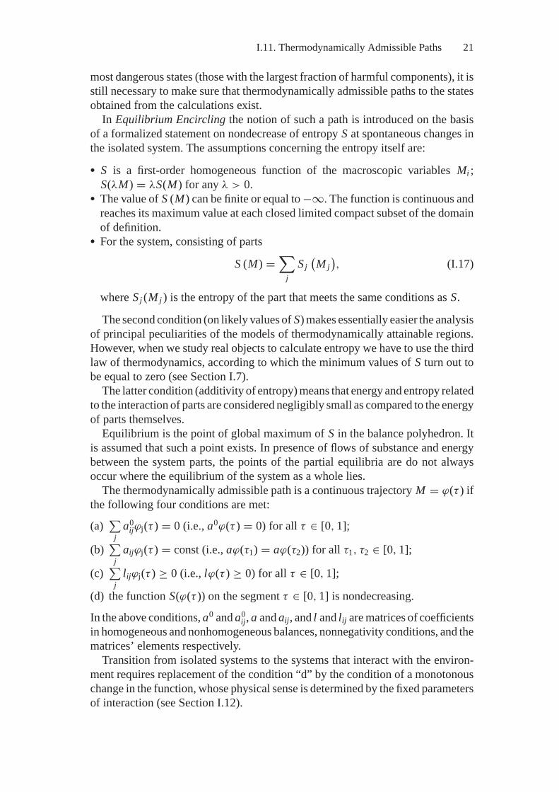
The thermodynamically admissible path is a continuous trajectory M = ϕ(τ ) ifthe following four conditions are met:
(a)∑
ja0
ijϕj(τ ) = 0 (i.e., a0ϕ(τ ) = 0) for all τ ∈ [0, 1];
(b)∑
jaijϕj(τ ) = const (i.e., aϕ(τ1) = aϕ(τ2)) for all τ1, τ2 ∈ [0, 1];
(c)∑
jlijϕj(τ ) ≥ 0 (i.e., lϕ(τ ) ≥ 0) for all τ ∈ [0, 1];
(d) the function S(ϕ(τ )) on the segment τ ∈ [0, 1] is nondecreasing.
In the above conditions, a0 and a0ij, a and aij, and l and lij are matrices of coefficients
in homogeneous and nonhomogeneous balances, nonnegativity conditions, and thematrices’ elements respectively.
Transition from isolated systems to the systems that interact with the environ-ment requires replacement of the condition “d” by the condition of a monotonouschange in the function, whose physical sense is determined by the fixed parametersof interaction (see Section I.12).
22 Introduction
In [58] the author gives examples of constructing admissible paths for the casewhere the reaction mechanism is set, and for a more general situation in which onlya list of reagents is known. The general technique was based on the transformationof the thermodynamic attainability region (a space of admissible paths) to a graph,namely a thermodynamic tree, and enabled one to obtain a number of interestingresults (see Sections I.13, 3.2 and 4.4).
The book Equilibrium Thermodynamics deals with the problems of admissiblepaths’ existence when modeling actually existing systems of a large dimensionalityfor both the case of absolute absence of the information on the process mechanismand the case in which there is fragmentary knowledge on the regions passed by thesystem trajectory in the space of compositions. Our book addresses the problemsof determining potential directions of motion in studies of principal peculiaritiesof thermodynamic and kinetic models and real objects in Sections 1.5, 3.2 and 4.4.
I.12. Thermodynamic Functions
A primary requirement of the set of variables to be applied, including the set offunctions, is that it should completely determine the state of the studied system,i.e., it should enable one to frame the system in by closed mathematical description.However, this requirement is certainly not the only one. Being closed, the modelsapplied should also possess an aggregate of valuable qualitative characteristics.
In principle we can construct the formal thermodynamics by building on fivevariables only: pressure P , volume V , temperature T , internal energy U and en-tropy S, as well as by two more quantities: heat q and work l, which can beexpressed via these variables. However, the vocabulary – at a minimum it con-tains only the listed terms—does not make it possible to see all the qualitativediversity of thermodynamic systems and processes, nor does it give clear explana-tions of their specific features or unfold clear and efficient theoretical principles.To perform a conceptual informal analysis of mathematical models of thermody-namics the list of the variables we use has to be essentially extended. Though,for every day communication in the home and in business, people need to knowabout 3,000 to 5,000 words, Pushkin’s language, which can express the subtlestshades of feelings and thoughts, contains about 20,000 units by the estimations ofphilologists.
It follows from the first and second laws of thermodynamics that, in an isolatedsystem at constant energy, the energy’s value in the course of any possible processdecreases; at maximum entropy (i.e., at equilibrium state), this energy cannot beused for performance of work or for heat transfer from one part of the system toanother. Thus, it becomes clear that to have a full picture of transformations inthe isolated system we must introduce variables that could characterize the valueof energy and the relationship between energy of individual parts and conditionsof interaction with each other. This circumstance made important the use in ther-modynamics of such functions as free Helmholtz energy F , enthalpy H , Gibbsenergy (free enthalpy) G, chemical potential μ, and some others.
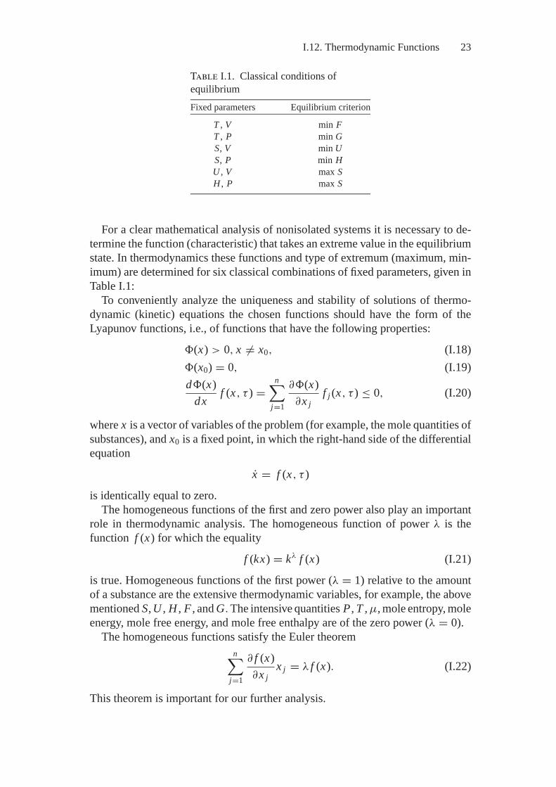
I.12. Thermodynamic Functions 23
Table I.1. Classical conditions ofequilibrium
Fixed parameters Equilibrium criterion
T , V min FT , P min GS, V min US, P min HU , V max SH , P max S
For a clear mathematical analysis of nonisolated systems it is necessary to de-termine the function (characteristic) that takes an extreme value in the equilibriumstate. In thermodynamics these functions and type of extremum (maximum, min-imum) are determined for six classical combinations of fixed parameters, given inTable I.1:
To conveniently analyze the uniqueness and stability of solutions of thermo-dynamic (kinetic) equations the chosen functions should have the form of theLyapunov functions, i.e., of functions that have the following properties:
(x) > 0, x �= x0, (I.18)
(x0) = 0, (I.19)
d(x)
dx f (x, τ ) =n∑
j=1
∂(x)
∂x jf j (x, τ ) ≤ 0, (I.20)
where x is a vector of variables of the problem (for example, the mole quantities ofsubstances), and x0 is a fixed point, in which the right-hand side of the differentialequation
x = f (x, τ )
is identically equal to zero.The homogeneous functions of the first and zero power also play an important
role in thermodynamic analysis. The homogeneous function of power λ is thefunction f (x) for which the equality
f (kx) = kλ f (x) (I.21)
is true. Homogeneous functions of the first power (λ = 1) relative to the amountof a substance are the extensive thermodynamic variables, for example, the abovementioned S, U , H , F , and G. The intensive quantities P , T , μ, mole entropy, moleenergy, mole free energy, and mole free enthalpy are of the zero power (λ = 0).
The homogeneous functions satisfy the Euler theoremn∑
j=1
∂ f (x)
∂x jx j = λ f (x). (I.22)
This theorem is important for our further analysis.
24 Introduction
Chapter 2 of this monograph discusses in detail the composition and specificfeatures of thermodynamic functions and their application to the analysis of modelsof chemical systems.
I.13. A Thermodynamic Tree and Space of Admissible Paths
Though the thermodynamic Lyapunov functions, set on polyhedrons of materialbalances, in most cases are either convex or approximated by convex curves withnegligible errors, the studies of peculiarities of the surfaces of these functions withrespect to large-dimensional systems represent a very complicated problem. Theissue is that, as applied to the problems discussed in this book, it turns out tobe necessary both to determine the location and properties of the final equilibriapoints and to find the partial equilibria that correspond to different compositionsof reaction mixture, admissible paths, and regions of thermodynamic attainabilityfrom the set initial states.
In mathematical programming (MP) (the theory of problems that search forextrema of functions) [19, 94, 142], algorithms are developed to describe theprocess of movement towards maximum or minimum points, which lie directlyon the surface of studied function. In [58] the author suggests a radically differentmethod of solving this problem, one that implies transforming a multidimensionaldomain of the function into a one-dimensional set—a graph in the form of atree, called by the authors “a thermodynamic tree”. The authors examine specificfeatures of the function’s behavior already on this graph.
Here, A.N. Gorban introduces the notions of thermodynamic preorder and ther-modynamic equivalence.
Preorder is defined as the condition in which x1 ≥ x2 if there exists a thermo-dynamically admissible path ϕ (τ ), τ = [0.1], such that ϕ (0) = x1, ϕ (1) = x2.
Thermodynamic equivalence is defined as the condition in which x1 ∼ x2 ifx1 ≥ x2 and x1 ≤ x2. The states x1 and x2 are comparable if x1 ≥ x2 or x1 ≤ x2.Comparable states x1 and x2 always belong to one balance polyhedron.
The identification of thermodynamically equivalent states on the balance poly-hedron results in a thermodynamic tree or a tree of entropy.
The condition of arcwise connectedness components is another very importantnotion for description of chemical systems by the “trees”, which was introducedin [58]. The component D\U (U a convex set) that contains the point x0 is anaggregate of all points x for which there is a continuous path in D\U that connectsx0 and x . Any two points lying in one arcwise connected component D\U can beconnected by continuous paths located in D\U .
In [58] it is shown that between the components exhibiting arcwise connected-ness in the initial polyhedron D and the thermodynamic tree Y there is a one-to-onecorrespondence. This makes it possible to map the whole set of thermodynamicallyadmissible paths from different initial points (states) and thermodynamic attain-ability regions on Y and to find on the tree the points with the known compositionand extreme concentrations of given substances, as well as to estimate the limits of
I.14. From Admissibility to Feasibility 25
change in the composition of reaction mixture at a given class of thermodynamicequivalence.
Chapters 3 and 4 of the present book repeat in brief the principles presented in[58] and an effort is made to further extend the ideas of the “tree” to devise thecomputational algorithms for analysis of really existing systems of large dimen-sionality. The main problem here is associated with the huge numbers of verticesand edges of trees that are obtained when modeling multicomponent chemicalmixtures.
I.14. From Admissibility to Feasibility
The estimation of what in principle may happen to a studied system is usuallynot sufficient to obtain a satisfactory result of the studies. It is always desirable toobtain more specific information on the opportunities and conditions of feasibilityof one or another probable event. The thermodynamics, as is known, is liberal andallows everything that is not contradictory to its first and second laws. To choosefrom an admissible set of processes and states those which are practically feasible,some additional nonthermodynamic initial data are needed. Because the latter arequite often unreliable, they have to be varied.
In G.K. Boreskov’s opinion [22], everything allowed by the thermodynamicscan be realized. The question is only how some desirable or undesirable state isattained. If it concerns the technological processes, the required results can beachieved either by choosing catalysts, the number of which is unlimited, or byregulating the parameters. If natural processes are the subject of the study, the rateof individual reactions of process mechanism is changed by the nature itself, whichpossesses an inexhaustible set of control means.
The difficulty, naturally, consists in revealing and describing those methods ofprocess implementation that are used by humans and nature. Unfortunately onecan find with certainty only fragmentary data. Mainly we employ assumptions thatrequire further analysis of their reliability.
Sometimes it turns out possible to set a part of the initial information in aprobabilistic form. For example, to forecast the air pollution in some region wecan estimate the probability of unfavorable combinations of meteorological factors(pressure, temperature, air humidity, wind speed) in terms of accumulation ofharmful substances. It is also possible to estimate roughly probabilities of limitingconditions of fuel combustion in energy plants. In some situations we can assumeequal probabilities for different sets of initial data. Yet, the dominating cases arethose for which we can estimate only the ranges of changes in the factors thataffect the course of the process studied.
Additional information is conveniently varied at an extreme formulationof the problems solved, particularly when the problems are described in theform of mathematical programming (MP). In this case within a single generalmodel, for example MEIS, it becomes easy to change composition of variables,form of objective functions, set of equality and inequality constraints, values,
26 Introduction
and the list of fixed parameters, formulas for calculation of thermodynamicfunctions.
The problem of constructing the model that takes into account the specific natureof a concrete studied process turns out physical-technical rather than mathematical.The involvement of additional constraints or variables into the problem statementcan certainly result in nonlinear balances, violation of the objective function surfaceconvexity, and some other effects. However, the main difficulty is in the formulationof the initial assumptions on the physics and chemistry of the process. Comparingthe results of modeling with the known published data on the processes, similar tothose studied, we can correct iteratively these assumptions and achieve plausibilityof the final result of the computational studies.
A comprehensive analysis of possible feasibility of complex processes certainlyrequires employment of other models besides MEIS. Thus, the use of the LMAequations (in thermodynamic form (I.16)) helps us estimate the impact of theprocess mechanism on the attainable states. Estimation of stability of the analyzedpartial equilibria can require direct application of kinetic models. The complexityof LMA and kinetic models mentioned in the previous sections makes us reduceessentially the list of substances for their construction, as compared to the MEIS-based description, which is also a nontrivial problem. Consideration for the impactof heat and mass transfer and hydrodynamics on the process can also call for theappropriate simplified models.
The problems outlined in this section are analyzed in the next sections of theIntroduction, in Section 4.5, and in Chapter 5, which is dedicated to the thermo-dynamics applications.
I.15. Constraints Imposed by the Reaction Mechanism
The monograph Equilibrium Encircling gives a theoretical analysis of reactionmechanism impact on thermodynamic attainability regions, and on partial andcomplete equilibria in chemical systems. The technique applied for the analysis isillustrated on the elementary example of isomerization in a closed system at con-stant temperature and volume. The applicability of the technique for the analysisof behavior of the open systems with nonequilibrium environment was also shown.Though the suggested algorithm does not possess high computational capabilities,it fosters understanding of the main patterns of equilibrium detour and facilitatescorrect construction of more complex models and algorithms.
Setting constraints on the process mechanism when we study multicomponentsystems calls for solution of a number of complicated problems.
First of all, we encounter the problem of determining the mechanism itself. In[58] “mechanism” means a list of elementary reactions set by stoichiometric equa-tions. If we regard as “elementary” those reactions that go forward in interaction(collision) of species (as it is usual to do), the list of such reactions for real techno-logical and natural processes is usually hard to describe due to its extensiveness.For example, in coal combustion just the components formed out of organic and
I.15. Constraints Imposed by the Reaction Mechanism 27
mineral parts of coal in more or less noticeable concentrations (assume more than10−8 mole/kg of the mixture) account for several hundreds species; the numberof elementary reactions is much larger. Recall that when solving environmentalproblems we may be interested in estimating concentrations of harmful ingredientswhen their fractions in the reaction mixture do not exceed 10−12–10−15. Setting acomplete list of elementary reactions here becomes unrealistic.
Equilibrium Encircling emphasizes the possibility of determining the elemen-tary character of reactions phenomenologically based on the form of the kineticequations for a unit of the reaction mixture volume,
x j =∑
s
(βs j − αs j
)ws (x, T ), (I.23)
where β and α are stoichiometric coefficients on the right-hand and left-hand sidesof the stoichiometric equation of the sth stage (reaction), respectively; and ws isa rate of the sth stage. Here the function form w = f (x, T ) was supposed to beknown. However, such knowledge turns out to be hard to come by even whenseveral tens or hundreds of overall reactions in a real process are regarded aselementary.
Therefore, when studying the large-dimensional systems, we can hope only forthe knowledge (still incomplete) of stoichiometric equations of principal overallreactions ∑
jα j A j =
∑j
β j A j , (I.24)
where A j are substance symbols.The mechanism represented by a system of equations of type (I.24) can obviously
be determined as a conditional “overall mechanism.”The next and apparently to a great extent nonformalized problem consists in
putting forward the hypothesis on such a mechanism. Its solution in each specificcase should be based on the available preliminary knowledge on the physics andchemistry of the process and depends on the researcher’s skills (see SectionsI.20, I.21).
And finally the third problem is associated with formalization of an assumedhypothesis in the form of separate blocks of the mathematical model to be applied.
If MEIS is chosen as a main tool for the study, the choice of a list of substances(the composition of the sought variables) turns out to be the simplest and mostnatural way to indirectly account for the mechanism.
In [83], attention is given to several algorithms for checking the hypothesis onthe process mechanism and to considering the assumed hypothesis in the analysisof the chemical systems’ behavior. In doing so MEIS was used along with thethermodynamic models on graphs specially intended for the analysis of mecha-nisms of chemical reactions. Further the problem of setting the constraints on themechanism is analyzed in Sections I.20 and in I.23–I.25 of the Introduction andin the body of the book.
28 Introduction
I.16. Constraints on Exchange
As mentioned above, most chemical-technological systems and practically all nat-ural systems are open. Even in cases where the processes taking place in themcan be studied using the models of closed systems, we still encounter problemsdescribing the mass-and-energy exchange with the environment.
As examples we can present here the problems of modeling atmospheric pollu-tion and state of indoor air environment.
The components of the atmosphere of any city or region are involved in thevarious processes of exchange with the heterogeneous environment: mass transferby the air flows from the neighboring regions, sorption (desorption) by groundsurface; solution in the aqueous medium; condensation (evaporation); and energyexchange with solar radiation, water, and terrestrial surface.
The exchange processes in ventilation and air conditioning systems in buildingsare distinguished by a similar variety. Here, first of all, absorption and extractionof harmful substances at the boundary surfaces and moisture condensation on thewindow apertures are of interest. Specific problems can appear when we modelair exchange in the production premises and in mines where formation of a largenumber of harmful and explosive ingredients and significant heat emission areoften observed.
The processes in furnaces (combustion chambers) of energy plants include sub-stance transfer (fuel, air, and combustion products) and heat exchange with heating(cooling) surfaces.
When studying the above and many other systems, description of the exchange(interaction) conditions with the environment can be made easier owing to a properchoice of the boundary between the considered system and its environment. Thus,conditionally including into the atmosphere the volumes of water and dry landadjacent to the atmosphere, we can substitute to a greater extent the modelingof the transfer processes by the modeling of the system equilibrium conditionswith an increased number of phases. In doing so, those additionally introducedmasses (surfaces, energies, etc.) should be large enough to run processes (chemicalreactions, sorption, solution, etc.) that involve atmospheric components.
Variation in the system composition at its modeling should certainly be sensiblycombined with imposition of additional equality and inequality constraints on theexchange processes. For example, constraints on the rate of oxygen diffusion tothe surface of an oxidized substance can be represented in the form of inequality
xO2 ≥ xbO2
, (I.25)
where xbO2
is the quantity of O2 that, according to the mass exchange conditions,can not enter into reaction. The constraint on the endothermal process of nitrogenoxide formation at fuel combustion in a system with fixed P and T is describedby the inequality
H ≤ H b, (I.26)
where H is the system’s enthalpy; H b is the fuel calorific value.
I.17. Constraints on Parameters 29
The latter inequality (I.26) can be interpreted as a constraint on the potentialrange of technological regulation of reaction mixture parameters. The set temper-ature and pressure can be maintained only when (I.26) is true.
I.17. Constraints on Parameters
We touched on problem of formulating the constraints on parameters in the previoussection, as it was relevant to the discussion of the exchange problem we addressedin that section. So, constant temperatures and pressure can be maintained onlywhen the chemical-technological process is run at definite rates of energy andmass transfer between the reacting mixture and the environment. In other words,T and P are regulated by this transfer.
Dependence of parameters on possibilities of regulation can be mathematicallyexpressed by additional constraints imposed along with the parameters determiningthe interaction of the system with the external environment. For example, for thesystems with fixed H and P it often turns out that it is useful to impose theconstraints
T ≥ T b or T ≤ T b. (I.27)
The first inequality in (I.27) takes into account using practical calculations (seeChapter 5) a possible decrease in furnace temperature due to endothermic reactionsof nitrogen oxide formation in them.
The choice of fixed parameters is not always obvious. For example, when study-ing the stationary process of fuel burning in a boiler furnace, we can assume thepressure and temperature in one of the furnace’s points are constant (this is mostlogical for the combustion completion area). However, in this case, as was ex-plained above, the equilibrium mixture formation can be accompanied by heatabsorption that exceeds the enthalpy of the initial fuel. Fixing of H and P in turncan lead to an unrealistically low temperature, at which the endothermic reactionsmay not be kinetically feasible.
Solution of the specified problems associated with the choice of initial physicalassumptions presumes, of course, correct mathematical formalization. An extrememodel, for example MEIS, should be constructed so that, on the one hand, there isa possibility for optimization and, on the other hand, all the relationships betweenthe variables that are required by the process physics are met.
Apparently, when determining the number of degrees of freedom f of multi-phase, multicomponent systems of large dimensionality, we cannot use the Gibbsrule of phases directly,
f = n − k − r + 2. (I.28)
For the systems with a disperse liquid phase in which the surface tension forcesshould be taken into account, number of degrees of freedom is given by
f = n − k − r + 3, (I.29)
30 Introduction
where n is the number of independent components (substances), k is the numberof independent reactions, and r is the number of phases.
Normally, without information (at least without quite full information) on theprocess mechanism, we can set neither k nor r . Prior to doing the calculations, itwould be hard for one to estimate which substances’ concentrations will be non-negligibly small, i.e., to estimate, in effect, what the system dimensionality will be.
Obviously, when we use extreme thermodynamic models, the phase rule shouldbe met automatically with accuracy as to the error in calculations due to observanceof equilibrium conditions.
Let us point out that, in using MEIS and other models of thermodynamic equi-libria, we digress from the classical definition of Gibbs. Namely, we regard “asystem component” as not an individual substance, but its amount in some phase.For example, if the water in a reaction mixture is present in gas and liquid phases,its concentration in the two phases is described by two separate variables. Suchan extension of the space of variables of the considered problem makes easier itsreduction to a convex programming problem.
These problems do not become more complicated in terms of computation whenthe inequality constraints on the parameters similar to (I.25)–(I.27) are includedinto the model.
I.18. Constraints on the Regions of Process Running
The problem of formalizing knowledge of the regions through which runs theprocess of the studied system’s relaxation to equilibrium is rather complicated.As is clear from the previous sections, sufficiently full data on both the reactionmechanism and the individual overall stages are hardly obtainable when modelingcomplex actual systems.
Available published and experimental data in the majority of cases enable us tospecify possible values for only a part of the composition vector components in theintermediate points of a process and do not allow the coordinates of these points tobe completely determined. Such scantiness of initial information naturally leadsto an increase in the number of computation options and in complexity of thecomputational experiments.
Chapter 5 presents examples of modeling regions of complex process running,a model that is based on a multistaged scheme of calculations. The scheme goeslike this. If we are to find a possible extreme concentration of the substance A andknow that at the intermediate stages of its formation substances C and B participatesuccessively (B at the stage after C) in the process, then we suppose the functionalrelationship
Aext = f (Bext(Cext)) (I.30)
to take place.
I.19. Stability and Sensitivity 31
Proceeding from (I.30) to determine Aext we first calculate Cext. Finding the com-position corresponding to the partial equilibrium with an extreme concentrationof C is assumed as necessary to finding Bext. And finally the composition with anextreme content of B is used to calculate Aext. MEIS, as an example, can be usedto perform all the calculations according to the above scheme.
Each stage of the computational experiment certainly supposes variation ofexternal and internal system parameters that seem for a researcher to be mostimportant in terms of attaining the sought extreme concentration. A rather fullpicture of relationships between the characteristics of the processes studied and themain influencing factors increase in the number of computations and in difficultiesin the analysis of results associated with a larger number of stages. If the subjectof the study is a natural process, the researcher determines conditions under whicha phenomenon of interest may take place. However, if consideration is given tothe chemical-technological process, the scientist then can determine the methodsof its regulation that lead to a desired result.
I.19. Stability and Sensitivity
The problems of stability of system motion along admissible paths and sensitivityof solution (partial equilibria that belong to these paths) were not consideredat length in either Equilibrium Encircling [58] or Equilibrium Thermodynamics[81]. At the same time the analysis of these problems is necessary if one is toestimate the realizability of the states that are considered using thermodynamicmodels.
Though a priori it is clear that accuracy of calculating the thermodynamicallyattainable points and estimating their feasibility depends on the quality of the initialinformation and real disturbances that are observed at some or another process,formalized statements of the problems are not obvious.
The statement of the sensitivity problem seems to be simpler than the stabilityproblem. In mathematical programming “sensitivity” is taken to mean the extentof change in the objective function as a result of small changes in the parametersof constraints. In linear programming the indices of sensitivity are the changes inthe dual estimations (Lagrange multipliers).
As applied to the problems discussed in this book an aggregate of the sensitivityindices used should obviously be essentially larger.
First of all, of interest are the changes in the composition of the studied equi-librium mixtures depending on the completeness (dimensionality) of the set listsof substances (the general list and the initial reagents). As is clear from the previ-ous text, the dimensionality of the variable space determines the possibility of theequilibrium detour, and with increase in this dimensionality the sought extremeconcentrations of the reaction mixture components may essentially rise. The prob-lems of analyzing the errors related to the setting of the list of substances areconsidered in Chapters 2, 4 and 5.
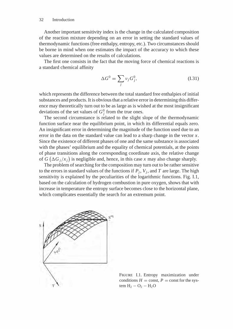
32 Introduction
Another important sensitivity index is the change in the calculated compositionof the reaction mixture depending on an error in setting the standard values ofthermodynamic functions (free enthalpy, entropy, etc.). Two circumstances shouldbe borne in mind when one estimates the impact of the accuracy to which thesevalues are determined on the results of calculations.
The first one consists in the fact that the moving force of chemical reactions isa standard chemical affinity
�G0 =∑
jν j G0
j , (I.31)
which represents the difference between the total standard free enthalpies of initialsubstances and products. It is obvious that a relative error in determining this differ-ence may theoretically turn out to be as large as is wished at the most insignificantdeviations of the set values of G0
j from the true ones.The second circumstance is related to the slight slope of the thermodynamic
function surface near the equilibrium point, in which its differential equals zero.An insignificant error in determining the magnitude of the function used due to anerror in the data on the standard value can lead to a sharp change in the vector x .Since the existence of different phases of one and the same substance is associatedwith the phases’ equilibrium and the equality of chemical potentials, at the pointsof phase transitions along the corresponding coordinate axis, the relative changeof G
(�G j/x j
)is negligible and, hence, in this case x may also change sharply.
The problem of searching for the composition may turn out to be rather sensitiveto the errors in standard values of the functions if Pj , Vj , and T are large. The highsensitivity is explained by the peculiarities of the logarithmic functions. Fig. I.1,based on the calculation of hydrogen combustion in pure oxygen, shows that withincrease in temperature the entropy surface becomes close to the horizontal plane,which complicates essentially the search for an extremum point.
S
T
Seq
x H 2O
Figure I.1. Entropy maximization underconditions H = const, P = const for the sys-tem H2 − O2 − H2O
I.20. The Art of the Possible: Idealized Modelsof Real Systems 33
It is also very important to estimate the sensitivity of solutions to the choiceof equations of state of the individual phases of a heterogeneous system andother analytical relationships (for example, for calculation of electrolyte activitycoefficients).
Passing to the stability problem let us explain the related practical problem.Suppose we are interested in producing the maximum amount of some substanceA by a given chemical process at set constraints on its purity. Naturally the questionarises: Will the considered process be stable, or will the concentrations of A andits purity inadmissibly change due to random variations in the quality of the initialraw material and parameters of the process? Similar problems may emerge whenone analyzes natural processes.
At formalization of such problems it is obviously desirable to consider stabilityby Lyapunov in accordance with the properties of the thermodynamic functionsused and in particular to study the stability problems of the autonomous systemequilibrium and stability of some of the variables. Here, problems arise of choosingthe disturbances, “some of the variables” and many others. They are discussed inSection 4.5.
When analyzing sensitivity problems and stability of solutions to thermody-namic problems we certainly need to take into account the errors and stability ofthe applied computational algorithms and computations.
I.20. The Art of the Possible: Idealized Modelsof Real Systems
The above description of the problems that emerge when modeling the regionsof attainability and partial equilibrium show quite clearly what the art of a re-searcher who deals with thermodynamic analysis of specific systems entails.This art should make it possible to explain the most important features of thestudied object even with insufficient information using the models of “liberal”thermodynamics (which allow everything that does not contradict its two mainlaws).
Certainly it is in principle impossible using thermodynamics alone to explaineverything that may be of interest to a researcher of one or another phenomenon.A good specialist should possess a set of specialized tools. A good theorist shouldhave a set of different theoretical (mathematical) models. As applied to chem-ical systems the special models are irreplaceable when calculating the time ofrelaxation toward equilibrium; when considering the nonequilibrium character as-sociated with distribution of microscopic variables that differ essentially from theequilibrium distribution; and in many other cases. However, it is desirable to ex-tend at most the application of thermodynamic models that are the simplest to usein computational experiments.
In the art of their application, including the areas that seem to be beyond thethermodynamics we can distinguish two constituents:
34 Introduction
1) the art of constructing a model that implies largely the art of simplification andidealization of real processes;
2) the art of carrying out computational experiments using the modelconstructed.
First, let us dwell on the art of constructing models and emphasize at once thatfortunately the well-constructed models find much wider use than the physicalassumptions that underlie these models. A small fall outside the limits determinedby the initial assumptions is observed in all the cases of modeling reality, since themodel is always a description of a real object with some errors, and it’s the realobject’s study through the model is always a deviation from assumptions madeby a researcher. However, the extent of violating the limits mainly depends on themodel’s designer.
Now, using the previous text let us try to set off individual components in theart of idealized description of real systems.
First of all, the choice of the modeled system type itself has the characteristicsof nontriviality and necessary for a researcher’s skill in accordance with what-ever the classification assumed in the thermodynamics is: isolated, open, closed,homogeneous, heterogeneous, ideal, or real.
Normally the studied objects represent open systems. However, if the researchercombines such systems with their environment in a number of cases, it is possibleto pass to the description of isolated systems. Neglect of the change in transitenergy flow passing through a system often allows for a correct use of the closedsystem model. Examples of these techniques were mentioned above. Decrease inthe number of phases when modeling a heterogeneous system can be illustrated inthe example of studying atmospheric processes; in that discussion, formation ofharmful substances on the surface of aerosols is described by their emergence in thehomogeneous medium. Equilibrium Thermodynamics [81] presents examples ofreal systems descriptions by ideal models: a real gas by an ideal gas; real solutionsby ideal solutions; the mixture of adsorbed substance on the surface of solid phaseby ideal surface gas.
The next component of the art is the skill of choosing the fixed parame-ters, i.e., the conditions of interaction between the system and the environ-ment. The nontriviality of this choice was already explained in Sections I.16 andI.17.
Use of equilibrium models for studies of principally nonequilibrium systemscertainly calls for intuition. The experience gained in such an art is discussed inmany sections of this book.
A most important condition of successful application of thermodynamic modelsis development of the skill in making up the lists of substances, which supposes ineach specific case the skill to guess the hidden peculiarities of the studied object.Certainly, it is necessary to correct preliminarily compiled list if the calculationsshow that the assumptions were not completely accurate. Simultaneously, it isdesirable to work at formalization of the analysis of a substance list’s impact onthe results of thermodynamic modeling.
I.21. The Art of the Possible: Methods for Calculation of Estimates 35
Finally, a subject of the art that is hardly subject to general recommendationsis consideration of nonthermodynamic factors: conditions of energy and massexchange, kinetic constraints, and so on.
In concluding this section let us point out that, in any case, the art of modelingshould be based on the already available knowledge of the specific subject of studyand on the experience derived from its analysis.
I.21. The Art of the Possible: Methods forCalculation of Estimates
Successful computational experiments call, first of all, for a good model or, thatwhich is even better, a set of models. However, this is certainly not enough. Thefollowing conditions should also be met:
� minimum required initial information should be prepared;� efficient computational algorithms should be devised and computer-aided com-
putational system on their basis should be created for laborious multivariantcalculations;
� a detailed program of conducting experiments should be elaborated;� the program should be strictly implemented;� results of calculations should be analyzed and the analysis should be thorough
and comprehensive enough to obtain profound conclusions.
Preparation of initial information includes nonformalized analysis of all acces-sible preliminary data on the studied object, concrete definition of the modelsused on their basis (composition of variables, objective function type, system ofconstraints) and some auxiliary calculations. The calculations, for example, canbe necessary to determine the standard values of thermodynamic functions if theycannot be determined from the available data bases. It is clear that the preparatorywork requires a researcher’s experience and knowledge.
A number of complicated problems are associated with creation of computa-tional algorithms. Though the models discussed in the book relate to the problemsof convex programming, cases where the functions to be optimized deviate fromstrict convexity or linearity are possible, and this increases the requirements onthe methods of calculations. Another computational complexity is determined bya very slight slope of optimized function surfaces near the final equilibrium andalong the individual axes near the partial equilibria, including the points of phasetransitions. The zones of the slight slope, as was mentioned above, can emerge dueto peculiarities of logarithmic functions as well.
Finally the principal problem of convergence and stability of computational al-gorithms arises when thermodynamic models are used for studies of environmentalcharacteristics of natural and chemical-technological processes; estimation of thecontent of harmful admixtures in materials of high purity; concentrations of highlyvaluable components in poor ores; and some other problems. Here we have to solve
36 Introduction
the systems of algebraic and transcendental equations with a large scatter in thevalues of sought variables (up to 12–15 orders of magnitudes), i.e., to say figura-tively, for example, weigh an elephant and an ant on the same scales. As an exampleof such “weighing” we can present the problem of estimating dioxin concentrationin the air, a dangerous dose of which is usually lower than 10–10 kg/kg.
It is clear that even the most efficient algorithms can be successfully used onlyif a computer-aided computational system is created on their basis and this systemprovides a user-friendly interface at multivariant calculations and their analysis.For construction of the system it is desirable to apply at most the available packagesof routine programs.
The key stage in a specific computational experiment with available models,algorithms realized on computers, and minimum required information is certainlythe development of the experiment’s program.
First of all we have to clearly formulate the objectives of the study, determiningwhat values should be determined to have an idea of potential favorable and unfa-vorable results of the studied process. After the objectives are set we can outline thelist of calculations to be made and the areas of variation in the initial information.Each step of the experiment calls for the choice of model and algorithm to be usedand determination of sensible accuracy of computations.
To reduce the number of variants to be calculated on computers and make easierthe analysis of the obtained information it is important to skillfully combine theuse of MP models with elementary analytical relationships. For example in [100]the study of the secondary pollutant formation in the air employed the formula
rjp = a j + b j�H 0xp , (I.32)
where
rjp = xextj p − x0
j
x0j
(I.33)
is a response of the atmosphere to the emission of the pth primary pollutant; a jand b j are coefficients; �H 0x
p is the change of enthalpy in reaction of the pthpollutant oxidation; xext
j p and x0j are extreme concentrations of the j th secondary
pollutant in the atmosphere polluted with the pth primary pollutant and in theclean (background) atmosphere, respectively.
Formula (I.32) allows one to sharply reduce the volume of thermodynamiccalculations when analyzing the secondary pollution of the atmosphere. Actually,in using MEIS it is only necessary to calculate the values of extreme concentrationsof the secondary pollutants in the background atmosphere (x0
j ). The technique ofderiving and using the relationships (I.32) and (I.33) is presented at length inSection 5.1.
A most subtle point in the analysis of thermodynamic modeling results is esti-mation of accuracy of the thermodynamic estimates themselves. Determining theaccuracy, we should bear in mind that, while involving various constraints in thethermodynamic models, thermodynamics still determines only limiting indices of
I.22. Models of Extreme Concentrations 37
the processes. Along with accuracy of the thermodynamics employed, we shouldestimate the accuracy of the initial information, algorithms, and computationalprocess. These points are discussed in Chapter 5.
I.22. Models of Extreme Concentrations
MEIS was the primary tool of the studies described in Equilibrium Thermodynam-ics. For fixed P and T it has the form of the following problem:
Find
max F (x, y) =
∑j∈J ext
c j x j∑j∈J 0
g j y j(I.34)
subject to
l∑j=1
M j y j = 1, (I.35)
Ax = b (y) , (I.36)
Ay = b (y) , (I.37)
αk∑j∈Jk
y j ≤ yk ≤ βk∑j∈Jk
y j , k ∈ K , (I.38)
Dt (y) = {x : x ≤ y} , (I.39)
G (x) = ∑j
G j (x) x j , (I.40)
x j ≥ 0, y j ≥ 0, (I.41)
where x = (x1 , . . . , xn
)Tis a vector of mole quantities of the reaction mixture com-
ponents; y = (y1 , . . . , yl
)Tis a vector of mole quantities of the initial reagents,
y ⊂ x ; J ext is a set of indices of components whose mixture’s extreme concentra-tion is to be determined; c j is a coefficient ranging the harmfulness (or any otherproperty) of the j th component of the vector x , c ≥ 0; J 0 is a set of initial compo-nent indices whose efficient use is of interest; g j is a coefficient ranging the valueof the j th initial reagent, g j ≥ 0; M is the mole mass; A is an m × n-dimensionalmatrix of contents of elements in the system components; α and β are coefficients;k is an index of inequality (or equality); K is a set of indices of initial reagents,on whose quantities the constraints are imposed; Jk is a set of indices of initialreagents considered in the kth constraint; Dt (y) is the region (the set) of thermo-dynamic attainability from the initial state; G and G j are the free enthalpy of thesystem and a mole of its j th component, respectively; and xeq is the compositionof reaction mixture in the point of global (final) equilibrium.
The form of the objective function (I.34) is chosen because we are often inter-ested in: the efficient use of the variable y’s individual components rather thanthe initial mixture of reagents as a whole. For example, when one studies the
38 Introduction
combustion processes it is more important to estimate the economic use capa-bilities of a deficient fuel than of the air. When the differences in the value ofthe initial components are not significant, the denominator of the expression inthe right-hand side of (I.34) can be taken equal to unity, i.e., we can use a linearobjective function.
Equation (I.35) is used to norm the numbers of the initial reagents relative to theunit of their mass. The matrix equations (I.36) and (I.37) express the condition ofconservation of a mole quantity of elements for each varied value of y. Inequalities(equalities) (I.38) are used to determine the admissible relationships between thevalues of different components of the vector y.
Expression (I.39) determines the thermodynamic attainability region at a fixedvalue of y. The sign ≤ within braces is taken to mean, in the thermodynamic sense(see Section I.13): x1 ≥ x2 if it is possible to pass from x1 to x2 by the continuoustrajectory, along which G (x) is monotonically nonincreasing. It is obvious that inDt (y) the inequalities G (xeq) ≤ G (x) ≤ G (y) are met.
The choice of formulas for computations of individual terms under the symbol ofsummation on the right-hand side of equality (I.40) depends on the initial physicalassumptions on the properties of the considered system, which are discussed indetail in Chapter 2.
The composition of variables of the model (I.34)–(I.41) is represented by twovectors x and y ⊂ x . This is rather important in terms of application, as it allows,based on the thermodynamic analysis, a strictly formalized solution to the problemon optimal composition of the initial reagents. The search for such a compositionusing the variant calculations may be laborious. Besides, strict optimization givesus a clearer idea on dependence of yext on the main influencing factors as comparedto the variant calculations.
Depending on the peculiarities of the studied system and specific statementof the problem, the model (I.34)–(I.41) can easily be supplemented by differ-ent equality and inequality constraints that reflect the conditions of energy andmass transfer, interactions with the environment, and impacts on the reactionmechanism.
A rather detailed analysis of mathematical features of MEIS and the problems ofupdating these models as applied to different types of thermodynamic systems waspresented in the book Equilibrium Thermodynamics. The main problem amongthose considered there consists in reducing MEIS to the problems of convex pro-gramming (CP). Its analysis implies consideration of three problems: 1) search forthe final equilibrium (xeq); 2) search for extreme concentrations (xext) at a fixedvalue of y; 3) search for the extremum point (yext, xext) of the function (I.34), i.e.,solution of a general problem (I.34)–(I.41).
The study of the first of the above problems in fact implies the analysis ofthermodynamic function convexity. A strict convexity (linearity by the axes thatcorrespond to the condensed phases) at some simplifying assumptions was provedfor additive systems with linear and nonlinear balances. For nonadditive hetero-geneous systems strict convexity was proved only for some areas of parameterchange, though the areas themselves were rather extensive.
I.23. Thermodynamics of Combustion 39
The second problem in the case of the thermodynamic function convexity con-sists in determination of the extremum of a linear form on the convex set ofconstraints. Its analysis revealed the conditions of (1) location of the point xext onthe boundary of the thermodynamic attainability region; (2) its coincidence withthe vertex that corresponds to the solution of the linear programming problem thatis obtained by excluding thermodynamic constraints (I.39) from the model; and(3) degeneration of solutions.
As applied to the third problem it was shown, based on qualitative speculationswithout strict formalization that at a search for maximum concentrations of theset of substances the objective function will much more likely be concave andthe problem reduce to CP. At the objective function minimization we obtain amulti-extreme problem of concave programming.
The above differentiation of mathematical models was carried out in accordancewith the probable composition of real systems to be modeled. The systems maycontain: ideal gas phase; real gases; plasma consisting of neutral active particles(radicals), ions, and electron gas; pure condensed substances; ideal solutions ofneutral substances and solutions of electrolytes; surface gas (two-dimensionalgas of adsorbed substances on the surface of adsorbent); substances in colloidal(dispersed) state, with the surfaces of their particles subject to the surface tensionforces, and other components.
The brief MEIS analysis presented in Equilibrium Thermodynamics showsclearly that many problems still remain unsolved. Further specification of math-ematical peculiarities and possibilities of reducing the models of extreme inter-mediate states to CP problems is important in terms of both improvement of thealgorithms applied to calculations and easier interpretation of the computationalexperiment results.
The next group of problems is associated with extension of MEIS application,in particular, with its applicability to systems with spatially nonhomogeneousstructure (see Sections I.23, I.25), concentrated solutions of electrolytes, electro-chemical systems with the sources of electromotive forces, and so on.
Chapter 2 of the book is entirely dedicated to the problems of further MEISdevelopment and application.
I.23. Thermodynamics of Combustion
The processes of fuel combustion and atmosphere pollution were presented manytimes as examples illustrating the problems that arise when modeling complicatedchemical systems of large dimensionality. Now we can try to systematize theproblems associated with the thermodynamic analysis of these processes. Theseproblems are interesting in terms of both theory and application.
Combustion thermodynamics and kinetics have been studied for more than100 years. First of all we should refer to a very short but excellent (in termsof profundity) thermodynamic analysis of hydrogen combustion in oxygen, whichwas presented in the book On Equilibrium of Heterogeneous Substances, by Gibbs
40 Introduction
[54]. Lacking both information on thermodynamic properties of substances anda computational tool, Gibbs managed to give a rather complete and qualitativepicture of the process. Discussing potential solutions of the derived systems ofequations he explained both the decrease in the reaction temperature due to waterdissociation and the presence of limited regions of explosion and burning.
Classical works on combustion kinetics were performed by N.N. Semenov[151, 152], Ya.B. Zeldovich [174, 175, 176], and others. The book Fluid Me-chanics, by L.D. Landau and E.M. Liftschitz [123] showed the possibilities ofusing thermodynamics in hydrodynamic analysis of the combustion process, inparticular, for calculation of amplitudes of detonation waves. In the last yearsintensive studies have been performed on the processes of harmful substance for-mation during fuel combustion in furnaces and combustion chambers of energyplants and vehicles [137, 165, 30, 169]. The main problem concerns determinationof concentrations in the combustion products of nitrogen oxides, sulfur oxides,carbon monoxide, and some other pollutants, using full-scale experiments andkinetic modeling.
The subject of the studies described in Equilibrium Thermodynamics [81] wasthermodynamic analysis of environmental characteristics of the combustion pro-cesses. The objectives of the thermodynamic analysis were: to reveal the efficiencyof the thermodynamics application in the study of real objects; to gain experiencein the joint application of thermodynamic and kinetic models and full-scale ex-periments; and to obtain useful application results. The processes of nitrogen andsulfur oxide formation in the stationary processes of the Kansk–Achinsk coal com-bustion in torch furnaces were considered in detail. The results of the calculationswere compared to the known published data and to the characteristics of real boilerunits.
The analysis showed that MEIS application made it possible: to understanddeeper the physics of the combustion process and suppression of NOx formationreactions by adjusting combustion modes; to estimate the potentialities of envi-ronmental updating of furnaces; and to obtain additional information for choosingconcrete methods of decreasing the formation of harmful ingredients in the fur-naces.
Increase in dimensionality of the problems to be solved (a list of consideredcomponents of the reaction mixture) when using MEIS as compared to kineticmodeling enabled one to find out the interrelations between the decrease in con-centrations of some pollutants and increase in the yields of the others (for exampledecrease of the NOx fraction in the reaction mixtures and increase in the CO frac-tion). Along with that the increase in dimensionality of the model allowed onecertainly to obtain a more complete idea on the range of the harmful products offuel combustion, which makes it easier to substantiate the choice of methods forregulation of the processes in furnaces.
At the same time the environmental analysis of combustion processes that waspresented in Equilibrium Thermodynamics revealed the problems and trends offurther development of thermodynamic methods in the studies on the impact offuel combustion technologies on nature.
I.24. Thermodynamics of the Atmosphere 41
First let us emphasize the inexhaustibility of the problems associated with mod-ification of models to simulate the processes in the furnaces of boiler units atmodern thermal power plants. These furnaces represent the largest chemical re-actors. Several hundred tons of fuel per hour can be burnt in them, their sizesreach 300–400 m2 in cross-section and 60–80 m in height. Here, both along themotion of gas or pulverized (in coal burners) mixture (usually vertically) and in theplane perpendicular to the motion, we observe drastic changes in the temperature,reaction mixture composition, and conditions of mass and energy transfer. Dif-ference in the temperature in the vertical direction is usually about 1000 degreesand differences in the horizontal sections are lower by approximately an order ofmagnitude. Thus, it is clear that powerful furnaces are spatially inhomogeneousstructures. The choice of models of such furnaces depends on both the specificfeatures of the combustion process to be modeled and the character of the problemto be solved.
Specific problems arise when we study the coal-burning reaction in the smallfixed-bed furnaces of industrial and municipal boilers and stoves. There we ob-serve periodic processes (fuel supply, normal combustion, rabbling, cleaning), forwhich change leads to sharp alterations in: the solid and gas phases, temperaturein the furnace, and conditions of harmful substances formation. Estimation ofenvironmental characteristics of small furnaces represents an important practicalproblem, since the contribution of these furnaces to environmental pollution isquite considerable.
The problems of the same complexity as those we have at description of periodiccombustion in the stationary plants arise certainly when using the equilibrium mod-els to model non-stationary processes in the engines of vehicles. The descriptionof forest fires in terms of thermodynamics is also interesting.
Modeling of combustion in the above types of the processes calls for modifi-cation of traditional MEIS, construction of principally new models of spatiallyinhomogeneous structures and improvement of computational algorithms. Spatialmodels are shortly discussed in Section I.25 and at length—in Chapters 2 and 3.Section 5.2 is entirely dedicated to the modeling of the combustion processes.
Section 5.3 addresses similar problems of fuel processing.
I.24. Thermodynamics of the Atmosphere
The difficulties of atmospheric thermodynamics are associated with the problemformulation itself, the construction of mathematical models, and with the devel-opment of computational algorithms.
The publications that contain thermodynamic interpretations of atmosphericprocesses date back at least to the early 20th century. The literature then wasmainly devoted to explanations of changes in the air parameters, emergence of airflows, formation of clouds and fogs, and some other phenomena. In the contextof our discussion, the works by Einstein on interaction of matter and radiation[39] are of interest, as is the article on the theory of opalescence [43], in which
42 Introduction
the analysis of partial equilibria (by Einstein’s terminology, “incompletely deter-mined in phenomenological sense”) is used to explain the blue color of the sky. Aclear thermodynamic analysis of atmospheric hydrodynamics is presented in theclassical textbook by Landau and Liftschitz [123].
However, up to now the thermodynamics has not been practically used for theanalysis of chemical transformations in the atmosphere and atmospheric pollutionby anthropogenic emissions. It is widely believed that due to low temperatureand hence extremely low rate of reactions the latter do not reach equilibrium andthermodynamic models turn out to be inapplicable in principle in atmosphericchemistry. Therefore, it is studied now mainly by the methods of kinetics andfull-scale experiments [12, 31, 36, 74, 128].
Equilibrium Thermodynamics [81] presents the problem of estimating the im-pact of anthropogenic emissions on air quality. The problem was formulated onthe basis of modeling the partial equilibria. Here we also have examples of de-termining maximum possible water vapor concentration in the atmosphere, limitsof carbon dioxide accumulation which account for its solution in the ocean, andforecasting the composition and concentrations of harmful substances, includingsecondary pollutants for given emissions.
The thermodynamic analysis of the air pollution got its further development in[84, 91, 100, 101]. These works reveal to some extent the advantages of thermody-namic models as compared to kinetic ones. Thus, the thermodynamics allows onein the course of a single computational process to simultaneously find the concen-trations of numerous pollutants (substances containing nitrogen, sulfur, chlorine,fluorine, etc.) yet the reactions of their formation turn out often very little studied.
Traditional MEIS, constructed as applied to closed systems with fixed P andT, underwent some definite tests as well as MEIS’s spatial modifications thatrepresent the description of chemical component distribution over the edges ofa graph, i.e., over the hydraulic circuit [91]. Application of the latter type of themodel is associated with a new statement of the problem, i.e., a search not only forthe composition of harmful substances, but for their distribution in space (one-,two-, and three-dimensional).
The results of the studies, where possible, were compared to the available pub-lished data. Quantitative comparisons were made only for the water vapor content,as there is a great amount of experimental material on this phenomenon. Highaccuracy has been mentioned before. At the same time, for the present we haveto be satisfied with the qualitative estimates of likelihood concerning the pictureof other microcomponents’ formation. Thus, thermodynamics modeling “con-firmed” existence of such known phenomena as acid rain, formation of peroxyacetyl nitrate (PAN), phosgene, and other pollutants experimentally detectable inthe atmosphere. The calculated concentrations of nitrogen dioxide appeared to beseveral orders of magnitude higher than those of monoxide, a result that is also inagreement with the experimental data.
Thermodynamic modeling also revealed the fact that the concentrations of mostof the secondary pollutants at the point xeq are practically equal to zero and reachnoticeable values only at the partial equilibria points. Certainly, it is impossible
I.25. Thermodynamic Modeling on Graphs 43
to determine by MEIS to what extent the stationary concentrations of individualsubstances corresponding to these equilibria are close to their plausible extremeconcentrations. Therefore, thermodynamic analysis may succeed only in estab-lishing the probability of dangerous concentrations of a number of pollutants inthe atmosphere, which itself is certainly not a matter of small importance.
The comparatively small experience gained in the thermodynamic modeling ofhuman impact on the atmosphere revealed the difficulties related to this modelingand outlined the objectives of further research.
A most interesting problem is the one of describing the processes that occur on amoist aerosol surface, which changes its sizes with time. Here, the need appears fora model of the phenomena of solution, sorption, and surface tension. The aerosolis considered an element of the unified thermodynamic system, i.e., a fixed amountof air.
Principal problems also have to be solved when we analyze photochemical pro-cesses that belong to the area of high energy chemistry. Besides, with sufficientlyhigh levels of description strictness they belong to relativistic thermodynamics.Description of the processes in terms of equilibria is related to the nontrivial sub-stantiation of admissibility of the accepted physical assumptions.
The thermodynamic modeling of accumulation of carbon dioxide and othergreenhouse gases in the atmosphere deserves extension and development. Here,we first of all need to specify the description of the air’s interaction with aqueoussurfaces and dry land.
Modeling of the processes of spatial distribution of harmful substances is so farat the initial stage of development. Here we have to determine a set of practicalproblems that arise, as well as what types of mathematical models we need toapply.
Touching upon the problem of improving the computational algorithms, weshould remind ourselves that it is precisely in the study of the atmospheric pollutionthat the problem of a huge scatter of values of variables is rather topical.
The thermodynamic modeling of atmospheric processes is considered in Sec-tion 5.1.
I.25. Thermodynamic Modeling on Graphs
The idea of thermodynamic analysis of kinetics of chemical reactions on graphsunfolds in the Equilibrium Encircling [58] which has already been discussed inSection I.13. Based on a graph, i.e., “the thermodynamic tree,” a qualitative descrip-tion of possible changes in the composition of a chemical system and admissiblepaths from arbitrary initial states is given in [58].
At the same time the idea of graphs as applied to the problems discussed inthis book can find other implementations as well. Along with the tree, the closed(cyclic) schemes are also of interest. In any case, transition from a multidimensionalto the one-dimensional space provides a number of advantages. The reduction ofthe sought functions to the functions of no more than two variables allows one
44 Introduction
to substantiate strictly the admissibility of applying differential equations (thePfaffian forms of one or two variables are always holonomic) and equilibriumthermodynamic methods. It is precisely the property of holonomy of infinitesimalincrements of functions (the Pfaffian forms) that was used by K. Caratheodory [27]and then by M. Born [23] to give macroscopic substantiation of thermodynamics.In Fluid Mechanics, by Landau and Liftschitz [123] there are a number of exampleson exclusion of the time variable from the description of one-dimensional flowsand solutions of typical dynamics problems by thermodynamic methods (suchas determination of amplitudes of different macroscopic quantities in the waveprocesses).
Addressing MP, one may assume that application of graphs essentially increasesit’s the method’s potential. Thus, the choice of MP methods can be interpreted asthe choice of a rule to be used at each step of the computational process to determinethe motion trajectory on the surface of the maximized (minimized) function in thedomain of its definition. When transforming this multidimensional domain to agraph the choice of a rule becomes at least, in some cases, more visible.
Efficiency of the multidimensional space transformation into a graph was re-vealed yet by Kirchhoff. Having obtained the formulas of current distributionin a round plate [111], he experimentally tested his theoretical conclusions onthe electric circuit, i.e., on the scheme that has a graph form, for which he de-rived his laws of current distribution. Such a test supposed agreement betweenthe values of variables that characterize electric fields at the points of a multi-dimensional region and on the graph. Having established for passive circuits theequivalence of the system of equations that describe the network conservationlaws and the problem of search for the minimum heat production, Kirchhoff infact showed the possibility of solving the extreme problems on graphs [108]. Forcomplex circuits, he suggested that the spanning tree be determined on these cir-cuit’s graphs [112], which could be used to determine the system of independentloops.
Maxwell solved the problem of current distribution on graphs by the method ofpotentials [129] and showed the equivalence of the latter to Kichhoff’s method.It is interesting that Maxwell’s development of the method of potentials for loopsalmost coincided in time with Gibbs’s introduction of the method of potentialsinto thermodynamics as applied to multidimensional spaces.
The problems of modeling thermodynamic systems on cyclic graphs were posedin [79] and considered in detail in Equilibrium Thermodynamics and later in [85].These works suggest three types of models:
� extreme thermodynamic models of flow (current) distribution in hydraulic andelectric circuits;
� graphical extreme models of chemical processes that are intended for determi-nation of final equilibria and based on the representation of a process in the formof an oriented graph whose arcs correspond to the flows of substances enteringinto some reaction or another, and the nodes are the points where the flows mergeand separate;
I.25. Thermodynamic Modeling on Graphs 45
� spatial MEIS modifications that are based on the representation of multidimen-sional, inhomogeneous spatial systems in graph form.
The models of hydraulic circuits were extended to circuits with multiphasechemically reacting flows. The topicality of researching such circuits is determinedby the need to solve many applied problems. For example:
� hydraulic calculations of chemical reactors;� calculation of operation modes for extended steam pipelines under conditions
of potential formation of condensate;� determination of conditions of sedimentation of heavy hydrocarbons in oil and
gas pipelines;� calculations of communications of energy plants with energy carriers of complex
composition.
Graphical models of chemical reactions were tested by the analysis of somesmall-dimensional systems, for example synthesis of methanol from the mixtureof carbon monoxide and hydrogen. It was revealed that these models could beapplied to study the impact of the reaction mechanism on the composition of finalproducts.
Based on the spatial MEIS, two problems were solved in [91]: distribution ofharmful substances in the vertical air column of the isothermic atmosphere; anddetermination of relationships between the pollution of outdoor air and indoor air.
A preliminary analysis of the mathematical peculiarities of the suggested modelswas carried out: The criteria of extremeness were determined; the possibilities ofreducing the problems solved to the convex programming problems were revealed;and the need was shown to describe the relationships between the head losses andflow rates in the flows with chemical transformations and phase transitions byalgebraic equations of no lower than the third power.
The studies to be planned for the future in thermodynamic modeling on graphsare: determination of new areas of efficient application of graphical models; mod-ification of the models according to the chosen purpose; analysis of their peculiar-ities and development of necessary computational algorithms; and solution of theapplied problems.
It is interesting to apply the models of heterogeneous hydraulic circuits to thestudies of ventilation and air conditioning systems on residential, public, and in-dustrial premises. This problem is rather topical in terms of its application. Wenow know that the traditional method of reducing the concentration of harmfulsubstances in buildings, a method that consisted of increasing the exchange ratio,may lead to a reverse effect due to the heavy pollution of “cleaning” air. To choosethe optimal methods of air conditioning it is necessary to combine the hydrauliccalculations of ventilation with the analysis of change in chemical composition ofthe atmosphere.
Development of graphical models of chemical reactions implies the elaborationof methods for determining partial equilibria with extreme concentrations of thegiven substances, i.e., the construction of models competing with MEIS, and the

46 Introduction
application of these models to determine reaction mechanisms—optimal in termsof yield of some substances.
The problems of constructing models for analysis of substance distribution intwo- and three-dimensional atmospheres, as well as for the analysis of combustionprocesses in spatially inhomogeneous systems, seem of top priority in the studiesof spatial MEIS modification.
The study of computational algorithms based on the idea of the thermodynamictree is certainly extremely interesting, as we mention in Section I.13.
The problems of graph-based modeling are discussed at length in Chapter 3 andSection 4.4.
1Principles of Equilibrium andExtremality in Mechanicsand Thermodynamics
A bearded sage once said that “there’s no motion.”His colleague strode before him. Stricken mute,He could no stronger argue or refute;All praised the cunning answer with devotion.Odd episode! But, men, I recollectAn old example from my mental journalThe sun before us strides in steps diurnalYet stubborn Galileo stands correct!
A.S. Pushkin
1.1. Principles of Equilibrium and Extremality in Mechanics
Thermodynamics theory, like physics in general, developed from mechanics, andthough the appearance of thermodynamics is associated with the analytical theoryof heat [51] and the kinetic theory of gases [21], its roots penetrate deep intomechanics. Therefore, prior to an analysis of the thermodynamic principles, it isuseful to discuss the basic principles of mechanics.
At the end of the 1960s the the beginning of the 1970s Heisenberg includedmechanics and thermodynamics along with statistical physics in the four closedtheories (models) of the modern physics. The two remaining are special theories ofrelativity and quantum mechanics. By “closed” Heisenberg meant the possibilityof an exhaustive and noncontradictory explanation for all the phenomena that relateto the subject of a relevant theory.
The main principles of mechanics and thermodynamics that allow a descriptionof the whole set of their applications can be called the principles of equilibriumand extremality.
Not dwelling on Archimedes formulation of the equilibrium laws as applied toindividual mechanisms and a body (his own, in this case) submerged in liquid,the story of the development of equilibrium principles should begin with GalileoGalilei, who employed the notion of uniform motion for formulation of his inertia
47
48 1. Principles of Equilibrium and Extremality in Mechanics and Thermodynamics
law. This motion can be seen as a continuous sequence of states in each of whichthe forces that act on the system are in equilibrium. It also becomes clear from theinertia law that the description (a model) of a uniform motion can be replaced bythe description (a model) of a state of rest, i.e., an equilibrium state. D’Alembertintroduced inertial force to describe the equilibrium state, which made it possibleto consider the nonuniform mechanical motions as those passing only throughsuch states.
It is natural to interpret the second and third laws of Newton in equilibriumterms. The second law determines equilibrium between the driving force and inertiaforce of the system at issue and the third law—equilibrium between the action andcounteraction.
However, a strictly formalized presentation of mechanics as a science on equi-libria and extrema was given by Lagrange in his famous “Mechanique analytique”[118]. He chose the equation of mechanical system equilibrium∑
jc j (x)dx j +
∑i
λi (ϕ)dϕi = 0, (1.1)
which was based on the principles of Galilei and d’Alembert, as the starting pointfor reconstructing all Newtonian mechanics.
The variables c, x , λ and ϕ are, respectively, a driving force, a coordinate, anunidentified multiplier (a bond resistance force) and bond deformation, and i andj are indices of driving forces and bonds.
Equation (1.1) is interesting for our analysis in many respects, and we will referto it many times in this book. First of all, it is used to reveal the interrelationsamong the principles of conservation, equilibrium, and extremality.
To reveal conservation of some quantity, let us note that each sum in the left-handside of (1.1) has the dimensionality of energy (or work). Hence, at an infinitesimaldeviation of a system from its equilibrium state, the work expended on its travelis equal to zero and the energy remains unchanged. The interpretation of the (1.1)represents the principle of virtual work (PVW).
Analyzing his equation, Lagrange revealed the connection between the equilib-rium and extremality principles from the fact that, if a left-hand side of (1.1) rep-resents a total differential of some function, the solution to the equilibrium searchproblem coincides with the solution to the problem of finding the extremum ofthis function. The extreme problem has the following form:
Find
extr(
L =∑
jc j (x)x j +
∑i
λi (ϕ)ϕi
), (1.2)
where L is the function that was subsequently called a Lagrange function.The assumption that an infinitesimal change in the function is a total differen-
tial in terms of physics means the mutually unique correspondence between thesystem’s state determined by the values x j and ϕi , and the value of function and,
1.1. Principles of Equilibrium and Extremality in Mechanics 49
hence, the potentiality of its field and equality,∮dL = 0. (1.3)
To facilitate further physical interpretation of the Lagrange equation, we trans-form it to the form
dT − d� = 0, (1.4)
where T and � are kinetic and potential energy of the system, respectively.The possibility of such a transformation is obvious: The work of the driving
forces c j is done through kinetic energy, and bond deformations affect the potentialenergy of the system. Naturally, the differentials of these energies have differentsigns as a decrease in one corresponds to an increase in the other. The systemsfor which equations (1.3) and (1.4) are met and the energy conservation lawsare reduced to the constancy of the sum T + � are called conservative systems,because no energy is dissipated in them.
In writing equation (1.1) Lagrange divided the forces applied to the mechanicalsystem into two groups: 1) those bringing the system to a motion (c j ), and 2) thoseresisting to this motion (λi ). The idea appeared to be excellent from a mathematicalviewpoint, as it allowed one both to formulate the problems of search for theextremes of type (1.2) and to pose the problems of a conditional extremum. Inthe latter case, the total work of driving forces is an objective function and theexpressions for the work of the bond deformation make up a system of constraints.Thus, Lagrange’s formulation of the equilibrium problem underlay the descriptionof modern problems of mathematical programming (MP) [19, 94, 142], which canbe defined as a mathematical theory of extrema.
Note that it seems natural to use MP in thermodynamic studies as thermody-namics is a science about extrema and equilibria.
Formulation of the equilibrium problems in MP terms facilitates their physical-mathematical interpretations. So, it becomes clear that the solution to an equi-librium problem corresponds to the saddle point of function L . Since the drivingforces c j try to move the system as far as possible from the initial state, and theresistance forces λi try to decrease the bond deformations, the equilibrium betweenc j and λi corresponds to maximum work of the former and minimum work of thelatter. Hence follows the possibility of dividing MP problems into ones of direct(maximization) and dual (minimization) problems, and the term “dual estimates”used by mathematicians as applied to λi become clear.
Based on the works by Maupertuis and Euler, Lagrange integrated (1.2) with re-spect to time and formulated mathematically a basic extreme principle of physics—a principle of least action (PLA):
δ J = δ
τ2∫τ1
Ldτ = δ
τ2∫τ1
(T − �)dτ = 0, (1.5)
where δ is a function variation, J is an action, and τ is time.
50 1. Principles of Equilibrium and Extremality in Mechanics and Thermodynamics
Those who developed variation (extreme) principles of mechanics [124, 141]introduced the key (in terms of thermodynamics) notions of reversible equilibriumprocesses into the science, though they did so without providing appropriate terms.Euler showed that PLA was met only for motion without friction, which, as is nowknown, causes irreversibility. Planck was the next to call the PLA a universalprinciple of equilibrium processes [139].
The most important property of the equilibrium systems was discovered byJacob Bernoulli, who showed that if any curve had the property of having either amaximum or a minimum, then any infinitesimal part of the curve had this property.This principle can be considered a prototype for formulations of extreme princi-ples in the theory of optimal control (by Pontryagin, Bellman, etc.). It followsfrom the principle that any state can be fixed in an equilibrium process. A prehis-tory of its attainment does not matter. Further optimal behavior of the system isdetermined only by this state. In the modern textbooks of macroscopic thermo-dynamics [20, 115, 117], equilibrium processes are usually defined as infinitelyslow and quasistatic. However, a property they possess (revealed in mechanics)—that of possibily setting off any intermediate state from a continuous curve of theprocess—is of principal importance for the modern analysis of thermodynamicmodels.
The Lagrange derivation of equation (1.5), optimal motion trajectory of a me-chanical system (PLA), from equation (1.1), optimal equilibrium state (PVW),and further study of the properties of these trajectories in mechanics, extendedthe understanding of interrelations between the models of rest and motion (firstrevealed by Galilei), and principal capabilities of thermodynamic modeling basedon elimintation of the time variable.
The use of a Lagrange function taking an extreme value for systems in equilib-rium states in the equations of motion in the form of difference between kinetic andpotential energy (T − �) allowed Helmholtz to define it as a “kinetic potential”or as a “free energy of the system”. The latter definition is of an explicitly thermo-dynamic character. Its essence is in the fact that for useful (efficient) movement, asystem need not use all the kinetic energy, but only the part that remains free fromthe work of bond deformation.
Mathematically the PLA development and application is associated with thecreation of the calculus of variations (CV), which is the study of the extreme tra-jectories of system motion. The ideology of CV can also be useful for mathematicalanalysis of thermodynamic problems.
1.2. Principles of Equilibrium and Extremalityin Thermodynamics
Thermodynamics, unlike mechanics, entails the study of systems undergoing trans-formations of substances and energy, as well as dissipation of the latter. It con-siders functions (heat q and work l) whose changes, as the system passes fromone state to another, depend on the path of the transition, and hence, heat and
1.2. Principles of Equilibrium and Extremality in Thermodynamics 51
work’a infinitesimal changes are not total differentials. Therefore, for thermody-namic systems the admissibility of the Lagrange assumption on correspondencebetween the problems of search for equilibrium and search for extremum falls farshort of being obvious.
The efforts put forth in reducing to mechanics wrote a number of importantpages in the history of the initial period of thermodynamic theory. Emergence ofthermodynamics is associated with the development of the kinetic theory of gases.In the course of this development, in the 1860s, Clausius discovered the existenceof a function, i.e., entropy, that is monotonically nondecreasing in isolated systems.Clausius, Boltzmann, and other researchers endeavored to explain this property ofentropy—the property of irreversibility of the natural processes. Their explanationwas based on the principles of mechanics, first among them, on the principle ofleast action (PLA). However, their efforts showed the principal impossibility ofreducing thermodynamics to mechanics and explaining the asymmetry of changeswith respect to time in thermodynamic systems by the models of conservativemechanic systems.
Clausius, Maxwell, Boltzmann, and Gibbs showed that the nature of irreversibil-ity can be revealed by passing from a deterministic to a probabilistic interpretationof physical laws.
Boltzmann, being unfortunately unfamiliar with the works of Russian math-ematicians, in fact applied the technique of Markov random processes and theLyapunov functions [140] to study the regularities of gas movement in a closedvessel. He chose as a base equation the kinetic equation for a gas consisting ofparticles of one kind. The equation was later assigned his name and has the form
∂ f∂τ
+ v∂ f∂r
+ 1m
F∂ f∂ϑ
=∫
( f ′ f ′1 − f f1)uσ (u, ϑ)d�dϑ1, (1.6)
where f (ϑ, r, τ ) is a function of distribution of gas molecules (particles) by veloc-ities ν and coordinates r ; ϑ and r are vectors (dϑ = dϑxdϑydϑz , dr = dxdydz);F(r, τ ) is the force acting on the particle (can depend on the velocity as well); mis particle mass; u = |ϑ − ϑ1| is a relative velocity of colliding particles; σ is adifferential effective cross-section of particle scattering into the solid angle d�;ϑ is an angle between a relative velocity and the line connecting the particles. Aprime on a function f in (1.6) indicates the state of the particles after collisionand the absence of a prime indicates their state before the collision; the index 1indicates particles colliding with those subject to distribution f .
The first term on the left-hand side of (1.6) is a change in the density of thenumber of particles in the element of a phase volume dϑdr per time; the second andthird terms characterize the changes in the distribution function due to movementof particles in space and the action of external forces, respectively. The integral ofcollisions on the right-hand side of (1.6) determines the change in f . This changeis related to the particles’ departure from the element of phase volume at the so-called “direct collisions” and replenishment of the volume with the particles thatunderwent “reverse” collisions.
52 1. Principles of Equilibrium and Extremality in Mechanics and Thermodynamics
Generally, the equation (1.6), the Boltzmann kinetic equation, reflects the bal-ance of the number of particles in the element of phase volume. The balance is main-tained at a change in f (ϑ, r, τ ) due to the motion of particles under the action of ex-ternal forces and collisions among them. Note that this equation takes into accountonly paired collisions and is true only for not too dense and not too rarefied gases.
For a gas in statistical equilibrium the integral of collisions vanishes and theMaxwell distribution by the velocities of particles
f (ϑ, r ) = A exp(
−mϑ2
21
kT
), (1.7)
becomes the solution to equation (1.6) in absence of a potential field, where k is aBoltzmann constant, A is a constant determined from the condition of normaliza-tion (the total number of particles for all possible states is equal to the total numberof particles in the system), and T is the absolute temperature.
For a system in the external potential field, the Maxwell distribution is replacedby the more general Boltzmann distribution,
f (ϑ, r ) = A exp(
−(
mϑ2
2 + U (r )) 1
kT
), (1.8)
where U (r ) is a potential energy of a particle in the external field.After we integrate the distribution function (1.8) by all the impulses of particles,
we can represent the Boltzmann distribution in the form of an equation that is usedto determine the density of the number of particles in the point r as
n(r ) = n0 exp(
−U (r )kT
), (1.9)
where n0 is a density of the number of particles that corresponds to the point inwhich U (r ) = 0.
For a mix of gases with particles of different mass, the Boltzmann distributionshows that the distribution of partial densities of particles for each component doesnot depend on the other components. The Gibbs distributions [55] together makeup the generalization of the Boltzmann distribution for nonideal systems.
Along with the interrelation revealed between the kinetics of gases and equilib-rium statistical distributions, Boltzmann’s analysis of the kinetic equation resultedin another very important conclusion for a closed and noncontradictory descriptionof thermodynamics. He formulated it in the form of the H -theorem, according towhich, for an isolated system, there is an H -function that monotonically decreaseswith time:
H =∫
h(r, τ )dr =∫∫
f (ϑ, r, τ ) ln f (ϑ, r, τ )dϑdr , (1.10)
where h(r, τ ) is a spatial density of the H -function, which means the local densityof entropy (S) with reversed sign and f (ϑ, r, τ ) satisfies the kinetic equation (1.6):
∂ H∂τ
=∫∫
(1 + ln f ) ∂ f∂τ
dϑdr . (1.11)
1.2. Principles of Equilibrium and Extremality in Thermodynamics 53
Substituting ∂ f∂τ
from (1.6) into (1.11) and symmetrizing the obtained expressionwith respect to the distribution function of colliding particles in direct and reversecollisions it can be shown that
∂ H∂τ
≤ 0. (1.12)
The H -function equals the gas entropy with a reverse sign and divided by k,therefore, the H -theorem expresses the law of entropy increase in isolated systems,i.e., it can be considered a formulation of the second law of thermodynamics. Math-ematically, the inequality (1.12) is equivalent to the more widely spread expression
dS ≥ 0. (1.13)The detailed conclusions and analysis of the presented relationships (1.6)–(1.12)
can be found in special monographs; for example, in the fifth [125] and tenth [127]volumes of Theoretical Physics, by Landau and Lifschitz. Here we use theserelationships to find the interrelations between the descriptions of motion and rest(equilibrium).
Bearing in mind that the equations of equilibrium distributions (1.7)–(1.9) haveno time variable τ and, hence, the equilibrium state can be determined from asimple calculation of probabilities, Boltzmann concluded that it was possibile toexclude the notion of time from thermodynamics as a science of equilibrium. Fromthe tendency of systems that satisfy the kinetic equation (1.6) to the minimum ofthe H -function (1.10) having the properties of a Lyapunov function, and, hence,towards the maximum of S, another conclusion follows relating to convergence ofthermodynamic problems to the mathematical problems of the search for extrema.This conclusion is very important to our analysis.
Assuming, along with the Markov character1 of the random motion process thatunderlies the derivation of the equation (1.6), the entropy additivity of the studiedthermodynamic system, it is easy to explain the third2 great Boltzmann equation:
S = k ln w. (1.14)
Indeed, if system entropy is a function of state probability (a fact that is clearfrom the previous text), and if the entropies of individual parts of this system do notdepend on the entropies of the others (also true, since the effects on a subsystem’sstate due to interactions between particles within is much stronger than interactionswith other subsystems), the following relationships turn out to be clear:
S = f (w), (1.15)
S =∑
jS j , (1.16)
w =∏
jw j . (1.17)
Equation (1.14) follows from (1.15)–(1.17).
1 The Markov character is that which describes how the evolution from a fixed state isindependent of the history of its attainment.2 The two others are (1.6) and (1.9).
54 1. Principles of Equilibrium and Extremality in Mechanics and Thermodynamics
Besides S, the other characteristic thermodynamic functions (those which takeextreme values under certain conditions of system interaction with the environ-ment) are also additive. These functions are internal energy U , enthalpy H , freeenergy of Helmholtz F , Gibbs energy (free enthalpy) G. The mathematical inter-dependencesies of U , H , F , and G with entropy are found using the differentialequations of thermodynamics.
The following equations [54] were chosen by Gibbs as the fundamental ther-modynamics equations (that is, they can be used to find all other necessaryrelationships):
At independent S, V , and x ,
dU = T dS − PdV +n∑
j=1μ j dx j ; (1.18)
at independent S, P and x ,
d H = T dS + V d P +n∑
j=1μ j dx j ; (1.19)
at independent T , V , and x ,
d F = −SdT + V d P +n∑
j=1μ j dx j ; (1.20)
at independent T , P , and x ,
dG = −SdT + V d P +n∑
j=1μ j dx j , (1.21)
where P is pressure, V is volume, μ is chemical potential, x is a mole quantity,and j = 1, . . . , n is an index of each component of the system.
As in the Lagrange equation of equilibrium (1.1), each term in equations (1.18)–(1.21) has dimensionality of energy (work). Each type of work done in the systemis determined by taking the product of corresponding potentials using conjugatedcoordinates.
Whereas Boltzmann drew on the example of ideal gas systems to show how itwas possible to pass from descriptions of motion (kinetics) to those of equilibriumstate, Gibbs extended those equilibrium principles to complex multiphase systems.
There have been a countless multitude of proofs to the trustworthiness of first theprinciples of equilibrium macroscopic thermodynamics presented systematicallyby Boltzmann and Gibbs. The theory has shown the highest scientific efficiencyfor more than a century.
However, the validity of using the thermodynamic principles of equilibrium andextremality for description of any macroscopic nonequilibrium and irreversibleprocesses (including the motions of a huge number of particles) has not yet beenstrictly proved. Indeed, when Boltzmann derived and used his kinetic equation(1.6) he supposed that motion and collision of individual particles obeyed the
1.2. Principles of Equilibrium and Extremality in Thermodynamics 55
laws of classical mechanics and were thus reversible, but he considered the finalresult of the process to be irreversible, i.e., attainment of a state with a minimumvalue of H -function (or a maximum of entropy3). Thus, his conclusion on theisolated systems’ tendency toward equilibrium turned out formally contradictoryto the initial assumptions of his work (which is thus referred to as “Boltzmann’sparadox”).
Gibbs in his book Statistical Mechanics [55], what was specially intended torationally substantiate macroscopic thermodynamic theory, also started with ana priori assumption on equilibrium distributions of probabilities of microscopicvariables (for example, particle energy).
In the context of the difficulties in substantiating the applicability of thermody-namic models to the studies of many real macroscopic systems the interpretationof equilibrium thermodynamics suggested by T.A. Afanasieva-Ehrenfest [2], C.Caratheodory [27] and M. Born [23] and based on the Pfaffian form technique, israther interesting.
The Pfaffian form
d� =∑
iXidxi , Xi = fi (x) (1.22)
is a generalized notion of the function differential, but in a general case its changedepends on the trajectory of transition from one point to another in the space ofindependent variables x . Hence, it may appear that∮
d�. (1.23)
Transition from the equation with the Pfaffian form to a differential equationbecomes possible in the case of a Pfaffian forms holonomicity, i.e., the existenceof such functions α(x) (integrating factors) for which
d f = α(x)d� (1.24)
is a total differential. Pfaffian forms of no more than two variables are alwaysholonomic. In thermodynamics the most important transformation of a Pfaffianform to the total differential is given by
1T
dq = dS, (1.25)
where is 1/T an integrating factor.It is precisely the possibility of transformation (1.25) that allows us, in a number
of cases, to explain the validity of formulating the equilibrium conditions forthermodynamic systems in the form where the left- and right-hand sides are equalto zero in the fundamental Gibbs equations (1.18)–(1.21). Besides, we start tobetter understand the significance of the inequality (1.13) with its left-hand side
3 It is impossible to simultaneously change the signs of velocities for a huge number ofparticles that make up a macroscopic system.
56 1. Principles of Equilibrium and Extremality in Mechanics and Thermodynamics
being a total differential of the function that has all the properties of potentials.Indeed, it represents the basic extreme thermodynamic principle, which assertsthe irreversibility of natural processes (the tendency to the entropy maximum, i.e.,the second law of thermodynamics). Hence, the behavior of this function can bedescribed by the models of equilibrium processes.
Certainly, it should be noted that the macroscopic substantiation of thermody-namics by Caratheodory and Born does not imply its reducibility to mechanics.In particular, the approach developed by them does not allow standard values ofthermodynamic functions (a mole, free energy, chemical potential, etc.) whosestatistical character is to be calculated.
A principal possibility of describing one or another problem in terms of equilib-rium thermodynamics allows the specific thermodynamic models to be constructedusing the equations analogous by form to the equilibrium equations of classicalmechanics. The thermodynamic potentials’ values, calculated on the basis of theprinciples of statistical physics or experimental data, can be substituted into theseequations similar to the manner that mechanical forces values are substituted. Fur-ther, in this book we use the formalism of mechanics in the construction of ourmodels many times, certainly bearing in mind the need to decide on the admissi-bility of such a technique in each specific case.
1.3. Thermodynamics and Models of Motion
Let us endeavor to derive the thermodynamic equations of some motion processesof macroscopic systems based on the principle formulated in the previous section,i.e., let us determine whether, if the studied system can be described in terms ofthermodynamic equilibria, it then becomes possible to apply the equations similarin form to the mechanics equations. Here we mean chemical transformations andtransfer processes (diffusion, thermal and electric conductivity, motion of viscousand ideal liquids, radiation). The relationships discussed below can be strictlysubstantiated only by using the Boltzmann kinetic equation and the statisticalprinciples. The “macroscopic” derivations of these relationships are useful here,as the subject of the present book is a macroscopic modeling of various physical-chemical processes, and macrodescription of relations among the processes studiedbecomes important for such a modeling.
Of special interest here is the use of the Lagrange equilibrium equation (1.1),which underlies mathematical programming. This is because the thermodynamicmodels we suggest are formulated in terms of mathematical programminf as well.
Figure 1.1 presents a conventional scheme of ties among thermodynamics andthe divisions of theoretical physics. A starting point of the scheme is certainly theclassical mechanics. It “feeds” all the other physical sciences. Thermodynamicsis a field of study connected directly with mechanics, statistical physics and kinet-ics. The latter here embraces both microscopic kinetics (based on the Boltzmannequation) and macroscopic kinetics (comprising chemical kinetics and transferprocesses). Unlike thermodynamics, which studies the states of rest of macro-scopic systems, kinetics deals with the study of motion toward these states. In
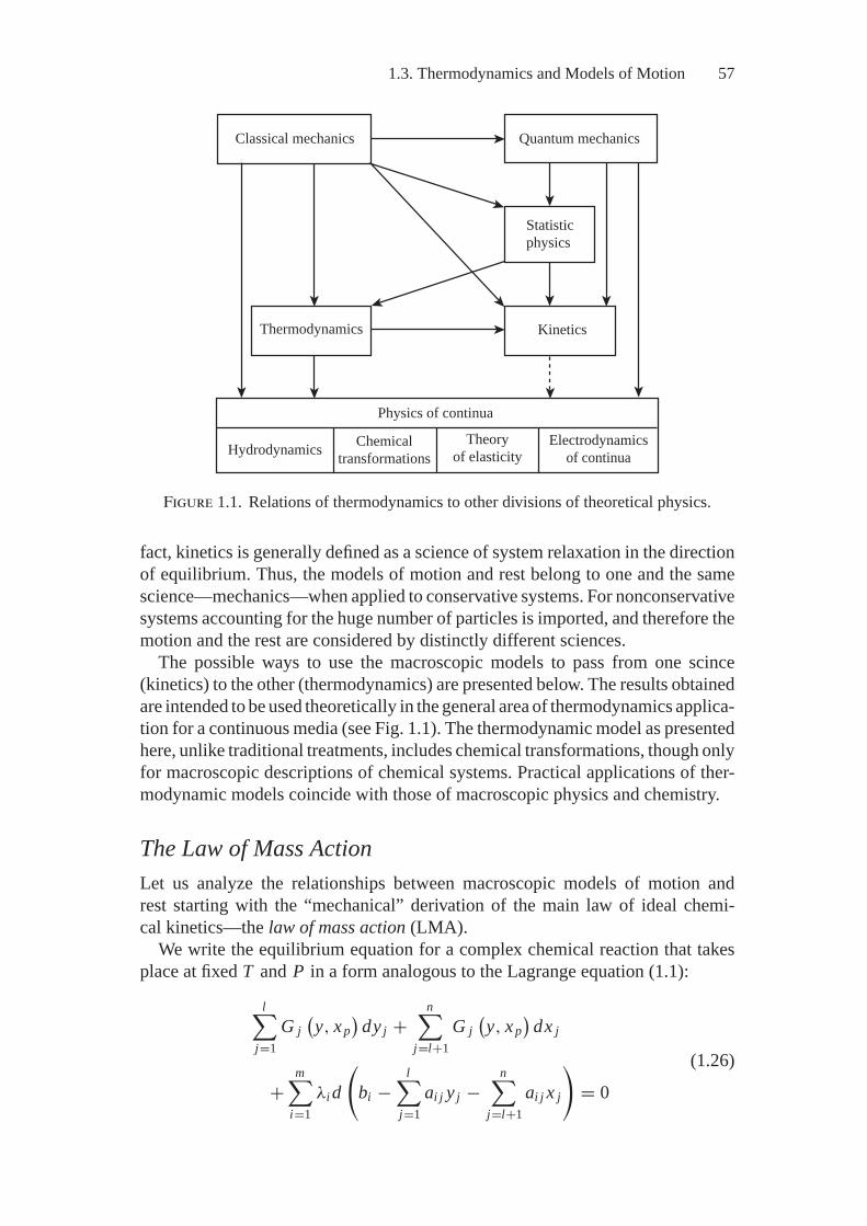
1.3. Thermodynamics and Models of Motion 57
Classical mechanics Quantum mechanics
Thermodynamics
Hydrodynamics
Statisticphysics
Kinetics
Chemicaltransformations
Theoryof elasticity
Electrodynamicsof continua
Physics of continua
Figure 1.1. Relations of thermodynamics to other divisions of theoretical physics.
fact, kinetics is generally defined as a science of system relaxation in the directionof equilibrium. Thus, the models of motion and rest belong to one and the samescience—mechanics—when applied to conservative systems. For nonconservativesystems accounting for the huge number of particles is imported, and therefore themotion and the rest are considered by distinctly different sciences.
The possible ways to use the macroscopic models to pass from one scince(kinetics) to the other (thermodynamics) are presented below. The results obtainedare intended to be used theoretically in the general area of thermodynamics applica-tion for a continuous media (see Fig. 1.1). The thermodynamic model as presentedhere, unlike traditional treatments, includes chemical transformations, though onlyfor macroscopic descriptions of chemical systems. Practical applications of ther-modynamic models coincide with those of macroscopic physics and chemistry.
The Law of Mass ActionLet us analyze the relationships between macroscopic models of motion andrest starting with the “mechanical” derivation of the main law of ideal chemi-cal kinetics—the law of mass action (LMA).
We write the equilibrium equation for a complex chemical reaction that takesplace at fixed T and P in a form analogous to the Lagrange equation (1.1):
l∑j=1
G j(y, xp
)dy j +
n∑j=l+1
G j(y, xp
)dx j
+m∑
i=1λi d
(bi −
l∑j=1
ai j y j −n∑
j=l+1ai j x j
)= 0
(1.26)
58 1. Principles of Equilibrium and Extremality in Mechanics and Thermodynamics
where G j is molar Gibbs energy of the j th reagent; y = y (y1, . . . , yl) andxp = (xl+1, . . . , xn) are vectors of mole quantities of initial reagents and reac-tion products, respectively; ai j is a mole quantity of the i th element in a mole ofthe j th component; and bi is the mole quantity of the i th element in the system.
Since the “bonds” (constant values bi ) in a chemical system are undistortable,the last sum in the left-hand side of equation (1.26) is identically equal to zero.Hence, the equation
l∑j=1
G j(y, xp
)dy j +
n∑j=l+1
G j(y, xp
)dx j = 0. (1.27)
turns out to be valid.Making the assumption that the detailed equilibrium principle is observed, we
pass from differentials to final differences and from the latter to stoichiometric co-efficients. Summing up these coefficients for all stages, in place of (1.27) we obtain
l∑j=1
G j(y, xp
)ν j +
n∑j=l+1
G j(y, xp
)ν j = 0, (1.28)
where ν j is a stoichiometric coefficient positive for the reaction products andnegative for the initial reagents.
For the ideal system the following relations are met:
G j(y, xp
) = G0j + RT ln
(P
yj
σ
), j = 1, . . . , l; (1.29)
G j(y, xp
) = G0j + RT ln
(P
x j
σ
), j = l + 1, . . . , n; (1.30)
σ =l∑
j=1y j +
n∑j=l+1
x j , (1.31)
where G0j is a standard value of molar Gibbs energy and; R is universal gas constant.
Therefore, equation (1.28) can be transformed to the form:l∑
j=1G0
jν j + RTl∑
j=1ν j ln
(P
yj
σ j
)+
n∑j=l+1
G0jν j + RT
n∑j=l+1
ν j ln(
Pyj
σ j
)= 0.
(1.32)Taking into account the signs of ν and introducing the notation
�G0 =n∑
j=l+1G0
jν j −l∑
j=1G0
jν j ,
we then make elementary transformations of the equation (1.32), obtaining:n∑
j=l+1ν j ln
(P
x j
σ
)−
l∑j=1
ν j ln(
Pyj
σ
)= −�G0
RT,
n∏j=l+1
(P
x j
σ
)ν jl∏
j=1
(P
yj
σ
)−ν j = exp(
−�G0
RT
). (1.33)
1.3. Thermodynamics and Models of Motion 59
SincePx j
σ= Pj , (1.34)
where Pj is a partial pressure of the j th component, the equation for the reactionequilibrium constant K p directly follows from (1.33):
K p =n∏
j=1Pν j
j = exp(
−�G0
RT
), (1.35)
i.e., a “thermodynamic” formulation of law of mass action (LMA).To pass to the “kinetic” formulation of LMA, we assume that the concentrations
of system components are equal to their partial pressures, i.e., P/σ = 1. That suchan assumption is possible is obvious, since the sizes of the system (a total molequantity) do not affect the mechanism of reaction. The assumption made, equation(1.33) can be replaced by the equivalent equation,
n∏j=l+1
(x j)ν j
l∏j=1
(y j)−ν j = exp
(−�G0
RT
), (1.36)
Taking into account that, in the equilibrium state, the rate of the forward reaction,
w+ = k+l∏
j=1yν j
j (1.37)
is equal to the rate of the reverse one,
w− = k−n∏
j=1+1xν j
j , (1.38)
i.e.
w+ = w− = w, (1.39)
we obtain the relationships
k+
k− =n∏
j=l+1
(x j)ν j
l∏j=1
(y j)−ν j = K p, (1.40)
That, together with equation (1.35), testify to the equivalence of the chemicalequilibrium principle to the law of mass action.
Arrhenius EquationNow let us try to use the Lagrange equation to clear out the type of equations thatdetermine the constant rates of reactions (k) that enter into the expressions (1.37)and (1.38).
60 1. Principles of Equilibrium and Extremality in Mechanics and Thermodynamics
Let us assume that nearing equilibrium the reaction rate w becomes constant(dxdτ
= const)
and equal to a mole quantity of the activated complex xcom that isformed per unit time. Then the equation of the chemical system equilibrium willhave the form
n−1∑j=1
G j(ya, xcom
)dy j + Gcom
(ya, xcom
)dxcom = 0, (1.41)
where y is a mole quantity of the initial reagents taking part in the reaction. For theabove reason this equation does not include the differential of bond deformation.Using the assumptions made when deriving LMA, we pass from (1.41) to theexpressions
n−1∑j=1
G j(ya, xcom
)ν j + Gcom
(ya, xcom
) = 0 (1.42)
andn−1∑j=1
(G0
j + RT ln(
Pya
j
σ
))ν j + G0
com + RT ln(
Pxcom
σ
)= 0, (1.43)
where σ =n−1∑j=1
ycj + xcom, and yc
j is the overall mole quantity of the i th reagent
in the initial state of the system. Based on the positivity of xcom (xcom > 0) andnegativity of ν j at j = 1, . . . , n − 1 (ν j < 0) and satisfaction of the equality
Pσ
= 1,
(the above made assumption) it follows from (1.43) that
xcom = w = e− �G0RT
n−1∏j=1
(ya
j)−ν j
, (1.44)
where
�G0 = G0com −
n−1∑j=1
G0jν j .
Since, according to LMA,
w = k∏
j
(yc
j)ν j
, (1.45)
it follows from (1.44) and (1.45) that
k = exp(
−�G0
RT
) n−1∏j=1
(ya
j)ν j
n−1∏j=1
(yc
j)−ν j
. (1.46)
1.3. Thermodynamics and Models of Motion 61
Assuming that an activated complex is formed adiabatically (entropy does notchange) we can pass from the equation (1.46) to the expression
k = exp(
− ERT
) n−1∏j=1
(ya
j)ν j
n−1∏j=1
(yc
j)−ν j
, (1.47)
where E is an activation energy.Finally, by introducing the notation
z =∏
j
(ya
j)ν j
∏j
(yc
j)−ν j
, (1.48)
we arrive at the generally accepted formulation of Arrhenius’ law
k = z exp(
− ERT
). (1.49)
The obtained relationships (1.48) and (1.49) to a certain extent reflect the realregularities. Thus, it is seen from (1.48) that pre-exponential multiplier z decreasesrapidly with an increase in reaction order (rise of ν j ), which is certainly true.However, here it is appropriate to emphasize that such “mechanical” conclusionsby no means imply reducibility of thermodynamics and kinetics to mechanics.For example, in this case when deriving equation (1.49) the standard Gibbs moleenergies were used as constant values in the initial equations. The values of theseenergies can be determined only by the principles of statistical physics. Eitherthe kinetic theory of gases, statistic relationships, or quantum chemistry methodsmay be needed, depending on the order of reactions and phase composition of thereacting medium to estimate with practical accuracy values z that depend on boththe energy of interacting molecules and their orientation in space.
The usefulness of mechanical interpretations in the cases similar to that at issue isrevealed when different macroscopic variables and relationships are combined intosingle closed models of complex physical-chemical systems. For example, in orderto qualitatively estimate the “impact” of thermodynamics on kinetics of chemicalprocesses, the Arrhenius equation, derived in terms of equilibria (mechanical andthermodynamic), can be used to include activated complexes, given as individualvariables, in thermodynamic models of chemical systems.
DiffusionEinstein established the main relationships for stationary diffusion at negligibleconcentrations of a diffusing substance in terms of a thermodynamic equilibriumbetween the forces affecting the moving flow. He did so in his classical works onBrownian motion [40–42]. Einstein considered as forces the osmotic pressure (adriving force) and the resistance force proportional to the velocity of particles. Here,following the idea of Einstein’s proof, we show the diffusion equation derivationusing the notion of chemical potential, widely applied later in the book, instead ofthe notion of osmotic pressure.
62 1. Principles of Equilibrium and Extremality in Mechanics and Thermodynamics
Let us suppose that the driving force is a derivative of the chemical potential ofdiffusing substance by the motion coordinate (l). Set off mentally a cross sectionin the moving flow and denote by indices 1 and 2 the mole quantities of movingparticles (x) before and after the cross section. Then the change in the chemicalpotentials associated with change in x will be found from the expression
�μ
RT=
[(ln x1 + ln
(Pσ
))−
(ln x2 + ln
(Pσ
))]x2 = x2 ln x1
x2(1.50)
In formulating equation (1.50) it was supposed that due to a small concentrationof the diffusing substance, σ on both sides of the set-off cross section would remainthe same. Now let us transform the expression in brackets in the right-hand sideof (1.50):
x2 ln x1
x2= x2 ln
(1 + �x
x2
)≈ x2
�xx2
= �x .
Hence,
�μ = RT�x . (1.51)
Passing from the final difference �x to the differential dx we can write thecondition of the thermodynamic equilibrium,
−RTdxdl
= a�xw, (1.52)
where a is a coefficient of proportionality and w is a diffusion rate.Einstein assumed the coefficient a to be equal to Nz (N being Avogadro’s number
and z, a particle’s resistance to motion) and determined z based on the assumptionthat the diffusing particles have the form of a sphere with radius r that exceedsessentially the radius of molecules in the solution (a carrier fluid). Under theseassumptions
z = 6πηr,
where η is a dynamic viscosity.From (1.52) it follows that
�xw = − RTa
dxdl
. (1.53)
The left hand-side of equation (1.53) represents the mole quantity of the sub-stance that passes through the cross section perpendicular to the fluid’s motionper second, i.e., a diffusion flow (J ), and the multiplier before the derivative inthe right-hand side equals the diffusion coefficient D. Hence, equation (1.53) isequivalent to the known equation of the Fick molecular diffusion law,
J = D∇x . (1.54)
1.3. Thermodynamics and Models of Motion 63
Darcy–Weisbach EquationThe hydrodynamics equation that determines head losses due to friction at liquidmotion in pipes is the Darcy–Weisbach equation. It has the form:
h = λlw2ρ
2d, (1.55)
where λ is a hydraulic friction coefficient, d and l are diameter and length of thepipe, w is an average velocity of the liquid motion, and ρ is density.
The equilibrium formulation of equation (1.55) is obvious. It reflects the equalityof a driving force (head) to a resistance force.
Hydraulic Shock in PipelinesIn the previous examples the description of motion was reduced to descriptions ofrest (equilibrium) as applied to the stationary processes. Now let us find from theequilibrium equation the pressure amplitude in a non-stationary wave process thatoccurs at fast valving off a pipeline along which the liquid moves. N. Zhukovskysolved this problem by the equations of ideal liquid motion in 1898 [178]. Theassumption on the ideality is obvious since a very steep increase in the pressuredoes not allow the friction forces to manifest themselves.
For a PVW (principle of virtual work)-based formulation of the problem, assumeadditionally that during an infinitesimal period of time dτ , the shock wave resultingfrom an instant braking of the flow propagates at a distance dl, where beyond thewave front the radius of the pipe increases and its walls become deformed. Thenthe Lagrange equilibrium equation can be written in the form
π (r + δr )2 Pdl − (ρ + δρ) π (r + δr )2 dldw
dτdl
−2π (r + δr ) dlPd (δr ) + λdϕ = 0 (1.56)
where P is maximum pressure in the pipeline, approximately taken to be equalto pressure increment; r and δr are the pipe radius and its increase due to shock,respectively; ρ and δρ are initial density of the liquid and its increase due tocompression, respectively; λ is a Lagrange multiplier, here interpreted as a stressin the pipe wall caused by its deformation; and ϕ is deformation.
The first term on the left-hand side of equation (1.56) is an infinitesimal work ofthe pressure force that acts on the liquid; the second term, the work of the inertialforce; the third, the pressure work related to a pipe radius increase; and the fourth,the work of the forces that appear in the wall due to its deformation.
Assuming that: 1) the work of the wall resistance (the third term) and the workof its deformation are negligibly small as compared to the first two terms in (1.56);2) δr and δρ are also negligibly small; and 3) an absolute value of dw equals an ini-tial velocity of the liquid flow, and taking into account the equality of the derivative
64 1. Principles of Equilibrium and Extremality in Mechanics and Thermodynamics
dldτ
to the shock wave velocity c, we obtain a simpler form of equation (1.56):
Pdl − ρcwdl = 0. (1.57)
Thus, follows the Zhukovsky equation for the hydraulic shock
P = ρcw. (1.58)
Certainly, if we tried to formulate equation (1.58) having expressed the velocityof the shock wave (sonic) c, as was done by Zhukovsky, in the form of a functionof the elastic properties of liquid and wall, we would not only fail to simplifyexpression (1.56), but we would have to specify the expressions for deformationof the walls and stresses in them. Thus, the initial equilibrium equation would be-come “more thermodynamic” owing to the consideration for the forces of differentnature.
However, even at an abstraction level chosen for the hydraulic shock description,i.e., at the assumption that the shock wave velocity equals the sonic velocity in a freefluid, the presented example illustrates a pool of equilibrium model capabilities.It shows that the models of “rest” appear to be efficient not only for analyses ofstationary processes but for the study of typical dynamics problems as well. If weare interested in the results of a non-stationary process (for example, shock waveamplitudes) rather than in the time of its duration, the equilibrium models (andthe relevance to extreme models) turn out to be rather convenient because of thesimplicity and clearness of their construction and interpretation. Additionally, wenote that when deriving (1.58) we implicitly use the assumption on the equilibriumdynamics, i.e., on the equilibrium of each state in the non-stationary process.
Ohm’s LawFor direct current Ohm’s law is known to have the form
U = RI, (1.59)
where U is the voltage applied to an electric circuit section; R is resistance, whichdepends on the conductor material, its geometry and temperature; and I is current.
Similar to the Darcy-Weisbach equation for liquid flow, equation (1.59) reflectsthe equilibrium (equality) of the driving force (U ) and the resistance force (IR).The linear dependence between I and U is explained by the linear dependencebetween the friction force that acts on the charge carriers and their velocity, whichis directly proportional to the current.
RadiationTo estimate the energy of gas radiation, let us use the macroscopic thermodynamicproof by Einstein as presented in one of his 1914 papers [38]. In this paper heused a conditional model that reflects chemically homogeneous gas in the formof a mixture of n different components, each characterized by its mole energy ε j .
1.3. Thermodynamics and Models of Motion 65
Following the idea of Einstein’s proof we use the notation of this book as appliedto the system maintained at a constant temperature and pressure.
When following the detailed balancing principle (Einstein used, but did notintroduce an appropriate term) for each reaction of formation (loss) of a componentwith energy other than the low (zero) level, we can write the equality
G0j + RT ln x j
σ= G0
0 + RT ln x0
σ, (1.60)
where lower index 0 refers to the component with zero energy level.From (1.60) it follows that
x j = x0 exp(
−G0j − G0
0
RT
). (1.61)
Assuming that the entropies of all the components are equal (the fluctuations ofelectrons in the atoms are reversible) we can pass from (1.61) to the Boltzmanndistribution equation
x j = x0 exp(− εi
RT
). (1.62)
Such an incidental macroscopic derivation of the Boltzmann distribution byEinstein is rather curious; however, it also does not allow one to consider themacroscopic substantiation of thermodynamics that is possible. Indeed, equa-tions (1.60)–(1.62) include those quantities that can be determined only usingthe statistic regularities.
Using equation (1.62) determining the value x j , Einstein wrote the expressionfor an average energy of the conditional mixture components
ε =
∞∑j=0
ε j x j
∞∑j=0
x j
. (1.63)
Assuming that ε j can take only discreet values proportional to Nhν (h is aPlanck constant, ν is a frequency of radiation), we can pass from (1.63) to theexpression
ε =
∞∑j=0
j Nhνx0e− jhν/kT
∞∑j=0
x0e− jhν/kT(1.64)
(in the exponent k = RN
).For further transformation of equation (1.64) we use the equation for a power
series expansion:
66 1. Principles of Equilibrium and Extremality in Mechanics and Thermodynamics
The numeration is
Nhνx0e−hν/kT(
1 + 2e−hν/kT + 3e−2hν/kT + · · ·)
= Nhνx0ehν/kT(ehν/kT − 1
)2 .
The denominator is
x0(
1 + e−hν/kT + e−2hν/kT + · · ·)
= x0ehν/kT(ehν/kT − 1
) .Thus we obtain the Planck equation for a monochromatic radiator (resonator),
ε = Nhν
ehν/kT − 1 . (1.65)
Taking into account that the ratio of the irradiated energy to the energy of aradiator is proportional to ν2 (see, for example, [49]) and integrating by ν, wewrite the expression
u =∞∫
0
ahν3dν
ehν/kT − 1 . (1.65a)
Having substituted
x = hν
kT,
we find
u = bT 4∞∫
0
x3dxex − 1 = σ T 4.4 (1.65b)
This is the Stephan-Boltzmann equation for emissivity of an absolutely blackbody.
Einstein evaluated the significance of the methodical approach to the deriva-tion of ε, noting that it followed from an approach recognizing no principaldifference between physical and chemical phenomena. In his opinion this macro-scopic thermodynamic approach was suitable for description of radioactive decay,diamagnetism, Brownian motion, and other phenomena. These statements ofEinstein apparently may serve as a logical conclusion to this section illustratingthe “almightniness” of thermodynamics.
1.4. Partial Thermodynamic Equilibria
The analysis of mechanical and thermodynamic equilibria that was presented inthe previous section of the chapter supposed that there was but one equilibrium
4 For the method of finding the integrals (1.65b) see in [65].
1.4. Partial Thermodynamic Equilibria 67
point in a system. However, as we stated in the Introduction, the capabilities ofthermodynamic analysis increase enormously in the transition from the searchfor the only point of the complete (final) equilibrium to the study of the wholethermodynamic attainability region, one that may include a continuous infiniteset of partial (by some parameters) equilibria. It is precisely when formulatingthe principally new problems that cannot be solved with manual calculation andtraditional approaches that the greatest effect is achieved by the use of moderncomputers. In this case we use not only their computational capabilities, but thepotentialities they offer in analyzing qualitatively complicated problems.
Let us consider the expediency of stating the problem of search for partialequilibria in more detail. The traditional analysis of thermodynamic equilibria isassociated either with determination of extrema of the appropriate function or withsolution of the LMA equations. However, when studying the technological andnatural processes, normally we are not interested in the extreme values of entropyor free energy but in the extreme concentrations of useful and harmful substancesformed in the course of a process. For example, when we compare different oilrefinery technologies it is important for us to know what maximum amount of lighthydrocarbons (petrol or kerosene) can be produced from a unit of the initial rawmaterial. When we study the environmental characteristics of the fuel combustionprocesses, the variables we seek are extreme concentrations of nitrogen oxides,sulfur oxides, carbon monoxide, benzpyrene, and other harmful substances. Suchcompositions may correspond not to the point of final equilibrium, but to partialequilibria that take place when the individual reactions slow down for some reasonsor do not run at all.
In Table 1.1 there are the examples of final equilibria calculations for severalprocesses of coal processing and methanol synthesis from the mixture of carbonmonoxide and hydrogen. They show that there are practically no target productsof these
Table 1.1 presents extreme concentrations of the indicated substances. Theseare substances that can form in reactors as a result of a naturally run process or aspecially arranged process in with relations among the rates of separate interactionsare artificially changed (for example, in the use of catalysts).
Substance transformation in atmospheric pollution is perhaps the best exampleof topicality of the problem of a search for partial equilibria as applied to the studyof natural phenomena. It is widely believed by specialists that thermodynamicsis principally irrelevant to atmospheric chemistry. Indeed, the traditional methodsof searching for final equilibria do not allow one to determine the results of theatmospheric processes. For example, according to these methods, all living naturein the oxidizing medium should turn mainly into carbon dioxide, water, and dilutesolution of the nitric acid [22]. This does not happen, however, the only reasonbeing the presence of extremely slow reactions under ambient conditions.
The concentrations of main atmospheric pollutants also turn out to be practicallyequal to zero in the final equilibrium state. It is seen in Table 1.2 that actuallyobservable dangerous concentrations of these substances in the air correspond tothe intermediate partial equilibria.
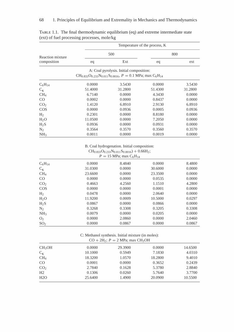
68 1. Principles of Equilibrium and Extremality in Mechanics and Thermodynamics
Table 1.1. The final thermodynamic equilibrium (eq) and extreme intermediate state(ext) of fuel processing processes, mole/kg
Temperature of the process, K
500 800Reaction mixturecomposition eq Ext eq ext
A: Coal pyrolysis. Initial composition:CH0.833O0.233N0.011S0.0016, P = 0.1 MPa; max C6H14
C6H14 0.0000 3.5430 0.0000 3.5430Ck 51.4000 31.2800 51.4300 31.2800CH4 6.7140 0.0000 4.3430 0.0000CO 0.0002 0.0000 0.8437 0.0000CO2 1.4120 6.8910 2.9130 6.8910COS 0.0000 0.0936 0.0005 0.0936H2 0.2301 0.0000 8.8180 0.0000H2O 11.0500 0.0000 7.2050 0.0000H2S 0.0936 0.0000 0.0931 0.0000N2 0.3564 0.3570 0.3560 0.3570NH3 0.0011 0.0000 0.0019 0.0000
B. Coal hydrogenation. Initial composition:CH0.833O0.233N0.011S0.0016) + 0.66H2;
P = 15 MPa; max C6H14
C6H14 0.0000 8.4840 0.0000 8.4800Ck 31.0300 0.0000 30.6000 0.0000CH4 23.6600 0.0000 23.3500 0.0000CO 0.0000 0.0000 0.0535 0.0000CO2 0.4663 4.2560 1.1510 4.2800COS 0.0000 0.0000 0.0001 0.0000H2 0.0478 0.0000 2.0640 0.0000H2O 11.9200 0.0009 10.5000 0.0297H2S 0.0867 0.0000 0.0866 0.0000N2 0.3268 0.3308 0.3205 0.3308NH3 0.0079 0.0000 0.0205 0.0000O2 0.0000 2.0860 0.0000 2.0460SO2 0.0000 0.0867 0.0000 0.0867
C: Methanol synthesis. Initial mixture (in moles):CO + 2H2; P = 2 MPa; max CH3OH
CH3OH 0.0000 29.3900 0.0000 14.6500Ck 10.1000 0.5949 7.1830 4.0310CH4 18.3200 1.0570 18.2800 9.4010CO 0.0001 0.0000 0.3652 0.2439CO2 2.7840 0.1628 5.3780 2.8840H2 0.1306 0.0260 5.7640 3.7700H2O 25.6400 1.4900 20.0900 10.5500
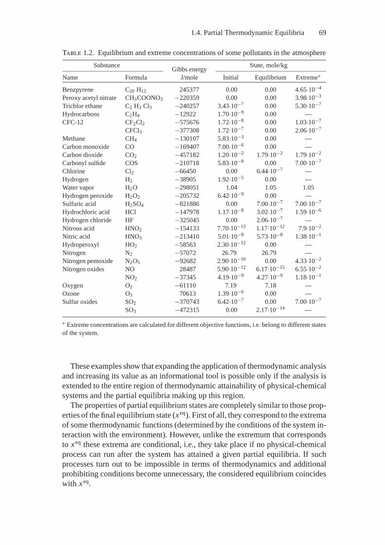
1.4. Partial Thermodynamic Equilibria 69
Table 1.2. Equilibrium and extreme concentrations of some pollutants in the atmosphereSubstance State, mole/kgGibbs energy
Name Formula J/mole Initial Equilibrium Extreme∗
Benzpyrene C20 H12 245377 0.00 0.00 4.65·10−4
Peroxy acetyl nitrate CH3COONO3 −220359 0.00 0.00 3.98·10−3
Trichlor ethane C2 H3 Cl3 −240257 3.43·10−7 0.00 5.30·10−7
Hydrocarbons C2H4 −12922 1.70·10−9 0.00 —CFC-12 CF2Cl2 −575676 1.72·10−8 0.00 1.03·10−7
CFCl3 −377308 1.72·10−7 0.00 2.06·10−7
Methane CH4 −130107 5.83·10−3 0.00 —Carbon monoxide CO −169407 7.00·10−6 0.00 —Carbon dioxide CO2 −457182 1.20·10−2 1.79·10−2 1.79·10−2
Carbonyl sulfide COS −210718 5.83·10−8 0.00 7.00·10−7
Chlorine Cl2 −66450 0.00 6.44·10−7 —Hydrogen H2 −38905 1.92·10−5 0.00 —Water vapor H2O −298051 1.04 1.05 1.05Hydrogen peroxide H2O2 −205732 6.42·10−9 0.00 —Sulfuric acid H2SO4 −821886 0.00 7.00·10−7 7.00·10−7
Hydrochloric acid HCl −147978 1.17·10−8 3.02·10−7 1.59·10−6
Hydrogen chloride HF −325045 0.00 2.06·10−7 —Nitrous acid HNO2 −154133 7.70·10−13 1.17·10−12 7.9·10−2
Nitric acid HNO3 −213410 5.01·10−8 5.73·10−8 1.38·10−1
Hydroperoxyl HO2 −58563 2.30·10−12 0.00 —Nitrogen N2 −57072 26.79 26.79 —Nitrogen pentoxide N2O5 −92682 2.90·10−10 0.00 4.33·10−2
Nitrogen oxides NO 28487 5.90·10−12 6.17·10−15 6.55·10−2
NO2 −37345 4.19·10−9 4.27·10−9 1.18·10−1
Oxygen O2 −61110 7.19 7.18 —Ozone O3 70613 1.39·10−6 0.00 —Sulfur oxides SO2 −370743 6.42·10−7 0.00 7.00·10−7
SO3 −472315 0.00 2.17·10−14 —
∗ Extreme concentrations are calculated for different objective functions, i.e. belong to different statesof the system.
These examples show that expanding the application of thermodynamic analysisand increasing its value as an informational tool is possible only if the analysis isextended to the entire region of thermodynamic attainability of physical-chemicalsystems and the partial equilibria making up this region.
The properties of partial equilibrium states are completely similar to those prop-erties of the final equilibrium state (xeq). First of all, they correspond to the extremaof some thermodynamic functions (determined by the conditions of the system in-teraction with the environment). However, unlike the extremum that correspondsto xeq these extrema are conditional, i.e., they take place if no physical-chemicalprocess can run after the system has attained a given partial equilibria. If suchprocesses turn out to be impossible in terms of thermodynamics and additionalprohibiting conditions become unnecessary, the considered equilibrium coincideswith xeq.
70 1. Principles of Equilibrium and Extremality in Mechanics and Thermodynamics
For partial equilibria, as well as for xeq, the requirement is met as regardingtheir attainability from the initial state of the system by the trajectory along whichthe characteristic function (that takes the extreme value in the point xeq) mono-tonically does not increase. Similar to xeq, the partial equilibria in accordancewith Boltzmann’s idea (see Section 1.2) can be found from a simple calculation ofprobabilities without studying the actual course of the process in time. Hence, therelations of classical equilibrium thermodynamics can also be used in the searchfor these equilibria.
Note that when we solve practical problems, partial rather than final equilibriaare calculated; this is because the lists of reactions or substances we would normallyconsider are never complete.
Dependence of the thermodynamic attainability regions of a chemical system,i.e., sets of equilibria attainable from it’s the system’s initial state, on the condi-tions of the processes run will be shown in the example taken from EquilibriumEncircling.
In [58] consideration is given to the reacting system that consists of three iso-mers: A1, A2 and A3. Since in isomerization reactions the number of species doesnot change the law of mass conservation for this system can be written in the form
x1 + x2 + x3 = |y| = const, x j ≥ 0. (1.66)
The assumptions were made that each of the system components is an ideal gasand in the state of final equilibrium their mole amounts are equal, i.e.,
xeq1 = xeq
2 = xeq3 . (1.67)
The algorithm for studying the equilibria attainable from the set y is illustrated byFig. 1.2, taken from [58] with some changes. Each triangle presented in the figureis a material balance polyhedron that meets condition (1.66). The triangles areequilateral, their heights are equal to |y| and sides to 2
√3 |y|/3. The vertices are the
states in which the system contains only one component. The initial compositionis determined by the vector y = (0, 0, 1)T (vertexA3). Figure 1.2a shows the pointof equilibrium xeq, line
G = (G0
j + RT ln(0.5P))
y (1.68)
(graphically constructed for T , P = const) and zones of thermodynamic unattain-ability from vertex A3: A1ab and A2bc (shaded). The nonshaded part of the figurerepresents the attainability region. Determination of the latter in this case is obvi-ous since line (1.68) due to condition (1.67) touches the edges at their mid pointsand these contact points are the points of minimum free Gibbs energy at edges.
The attainability regions in Figures 1.2 a–d are shown for four given mechanismsof the process (depending on the catalysts chosen or some other effects on thesystem):
a) A1 � A2 � A3;b) A2 � A1 � A3;c) A1 � A2 � A3 � A1;d) A1 � A2, A1 � A3, A1 + A2 � 2A3
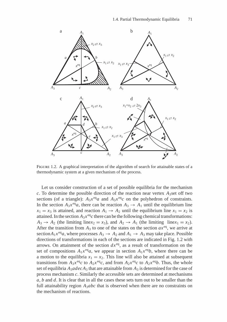
1.4. Partial Thermodynamic Equilibria 71
a b
dc
a b
c
a b
c
e
d
xeq xeq
xeqxeq
x2 x3
x2 x3 2x3
x1 x3
x1 x3
x1 x2
x1 x2
x1 x2
x1 x2
A2A3
x1+x2
A1A1
A3 A2
A3A2A3
A1 A1
A2
Figure 1.2. A graphical interpretation of the algorithm of search for attainable states of athermodynamic system at a given mechanism of the process.
Let us consider construction of a set of possible equilibria for the mechanismc. To determine the possible direction of the reaction near vertex A3set off twosections (of a triangle): A3xeqa and A3xeqc on the polyhedron of constraints.In the section A3xeqa, there can be reaction A3 → A1 until the equilibrium linex1 = x3 is attained, and reaction A1 → A2 until the equilibrium line x1 = x2 isattained. In the section A3xeqc there can be the following chemical transformations:A3 → A2 (the limiting linex2 = x3), and A2 → A1 (the limiting linex1 = x2).After the transition from A3 to one of the states on the section axeq, we arrive atsectionA1xeqa, where processes A3 → A2 and A1 → A3 may take place. Possibledirections of transformations in each of the sections are indicated in Fig. 1.2 witharrows. On attainment of the section dxeq, as a result of transformation on theset of compositions A1xeqa, we appear in section A1xeqb, where there can bea motion to the equilibria x1 = x2. This line will also be attained at subsequenttransitions from A3xeqc to A2xeqc, and from A2xeqc to A2xeqb. Thus, the wholeset of equilibria A3adecA3 that are attainable from A3 is determined for the case ofprocess mechanism c. Similarly the accessible sets are determined at mechanismsa, b and d. It is clear that in all the cases these sets turn out to be smaller than thefull attainability region A3abc that is observed when there are no constraints onthe mechanism of reactions.
72 1. Principles of Equilibrium and Extremality in Mechanics and Thermodynamics
Some time after the above work was done, a similar algorithm of search for theattainable equilibria was considered in the papers by R. Shinnar et al. [154, 155].
The possibility of finding the thermodynamic attainability regions suggests an-other tempting area of inquiry: the problem of determining in these regions thepoints that correspond to extreme concentrations of harmful or useful substancesof interest to a researcher. An analysis of this problem—one that goes beyond thetraditional methods of equilibrium thermodynamics—is the subject of the studypresented next.
1.5. A Thermodynamic Analysis of theChemical Kinetics Equations
The main content of this book is reduced to a direct application of equilibrium (ther-modynamics) models for the analysis of various natural and technological systems.However, thermodynamics can also be used to interpret and transform the motionequations. When so used, it allows reserchers a deeper understanding of motionequations and an easier solution to them. Such a thermodynamic method—studyingthe kinetics of chemical reactions—unfolds in the book Equilibrium Encircling.
Equilibrium Encircling contains a brief comparative analysis of formalismsof kinetics and thermodynamics, it reveals the interrelations between these for-malisms; and it offers the conditions of coordinating the kinetic and thermody-namic models. The possibility of simplifying the motion equations (excluding“fast” variables, use of local potentials) is based on the thermodynamic principleof entropy maximum. The applicability of the principle of detailed balancing inmacroscopic kinetics under condition of microreversibility has been substantiated;the idea of analyzing the direct problems of kinetics when incomplete informationis only available, basing the analysis on thermodynamic principles, has been putforward. The method of balance polyhedron transformation into a one-dimensionalcontinuum, i.e., a thermodynamic tree, has been suggested. The method makes itpossible to determine the substance compositions attained in the course of a chem-ical process. The technique has been developed to determine a multitude of steadystates in open systems.
The geometrical technique of constructing thermodynamic trees used in theEquilibrium Encircling can be applied in thermodynamic modeling. It is discussedin Sections 3.2 and 4.4. This section presents briefly the contents of the second,third and sixth chapters of the book by A.N. Gorban [58], which are devotedto coordinating kinetics with thermodynamics, and to applying thermodynamicprinciples to the analysis and solution of the kinetic equations. Understanding thecontents of these chapters is necessary if the reader is to correctly construct anduse the thermodynamic models discussed below.
Assumptions, Notions, and Nomenclature UsedExcept for a few exceptions, Equilibrium Encircling addresses the ideal systemswhose kinetics follow the law of mass action. Complex reactions in these systems
1.5. A Thermodynamic Analysis of the Chemical Kinetics Equations 73
represent an aggregate of simple (elementary) ones. Each elementary reaction isset by its stoichiometric equation
α1 A1 + α2 A2 + · · · + αn An � β1 A1 + β2 A2 + · · · + βn An, (1.69)
where A j are symbols of the substances; α j , β j are stoichiometric coefficients–integers that show how many molecules of A j are involved in one act of theelementary reaction as an initial reagent (α j ) and as a product (β j ). Both forwardand reverse reactions are written in (1.69). For the reverse reaction β j is the numberof molecules A j taking part in one act of reaction as an initial reagent; α j is thenumber of molecules A j that are produced in one act of the reaction as a product.
Each elementary process r is assigned to its stoichiometric vector γr with com-ponents γr j = βr j − αr j . Additionally, the elementary process is characterized byan extensive quantity Vr ≥ 0 (i.e., the volume of the process), and the intensivequantity wr ≥ 0, the process rate. The value V that characterizes the size of theregion in which the process takes place is called a volume conventionally. In spe-cific cases Vr can be a volume, a surface area, or the number of active centers ofcatalysts.
The rates of the forward (w+) and reverse (w−) reactions based on the LMAare determined from the equations
w+ = k+(T )n∏
j=1cα j
j , w− = k−(T )n∏
j=1cβ j
j , (1.70)
where c j is a concentration of the j th substance, and k± are the rate constants.The rate of the stage (the reverse elementary reaction (1.69)) is
ws = w+s − w−
s . (1.71)
The thermodynamic ideality of the considered system is determined by the formof the expression for the chemical potential,
μ j = μ0j + RT ln c j . (1.72)
Note, that in equations (1.70) and (1.72) and below in this section, unlike in therest of the book, along with the main variable (x), concentration c j is the molequantity of the j th component. Specifically, c j is the number of species (moles)of the j th component in a unit of V . This is to preserve the form of analyticalrelationships used in the Equilibrium Encircling. Following the rigor (found ib thatbook), for the antilog in (1.72), instead of c j we are right to use the dimensionlessratio c j
c0j, where c0
j is a concentration of the j th component in a standard state that
is taken to be equal to unity. In this case, the correspondence of equation (1.72)to equations (1.29) and (1.30) becomes clear. In those equations the antilogs arethe ratios of partial pressures to the ideal gas’ standard pressure, considered to beequal to unity.
74 1. Principles of Equilibrium and Extremality in Mechanics and Thermodynamics
The Schemes of Formal Thermodynamics and KineticsBefore discussing the problems of coordinating the motion models with equilib-rium models let us briefly consider the models themselves, i.e., formal descriptionsof thermodynamics and kinetics.
Suppose that the subject of a study is isolated systems. The study of the non-isolated system with equilibrium environment is reduceable to the analysis of aminimum isolated system, including the given one. The thermodynamic descrip-tion of the system, if specified, comprises the followings: the list of macroscopicvariables, a system of balance equations, a system of balance inequalities, andentropy as a function of macroscopic variables.
Denote the macroscopic variables as M j ( j = 1, . . . , n), and the vector withcomponents M j as M . The values of variables M j completely determine the sys-tem’s states. The choice of the main macroscopic variables for a specific system isfar from a trivial problem, but if the choice is made correctly we can consider anymacroscopic quantity a function of M . Let us identify vector M and a system’sstate.
Balance equations can be homogeneous:∑i
agi j M j = 0, ag M = 0, (1.73)
or nonhomogeneous:∑i
ai j M j = bi = const, aM = b = const. (1.74)
The balance of electric charges (the electric neutrality equation) can exemplifyequations of the first type. Presence of the relationships of type (1.73) means thatthe variables M j are not independent. Examples of equations of the second groupare balances of mass, energy, surface, etc. The values of the right-hand sides of(1.74) in the isolated system do not change with time. If it is possible to pass fromM1 to M2, then aM1 = b = aM2.
As a rule, besides balance equations, there are balance inequalities; for example,conditions of nonnegativity of variables (concentrations, volumes, etc.) expressedin general use:
M ≥ 0. (1.75)
Recall that the inequality x ≥ 0 for the vector x implies x j ≥ 0 for all coordinates x .The system of balance equations (1.73) and (1.74), and balance inequalities
(1.75) define a convex set in Euclidean space Rn , which is a balance polyhedron D.Entropy S is a homogeneous function of the first order of macroscopic variables
M j : S(kM) = kS(M) for any k larger than zero. It reaches maximum in the do-main D and is twice continuously differentiable. Equilibrium is the point of globalmaximum of S in a balance polyhedron. It is supposed to be an interior point of D.The metastable state represents a local maximum of S in D. Often, but not always,
1.5. A Thermodynamic Analysis of the Chemical Kinetics Equations 75
the condition of concavity [72] is met:
xT[
∂2S∂Mi∂M j
]x ≤ 0, x ∈ Rn, ax = 0, x �= 0, S(M) > −∞. (1.76)
The condition ax = 0 means that x belongs to the balance plane that passes throughzero. In D the conjugate variables μ j (M) = −∂S(M)
∂M jare determined. In the
equilibrium point
μ j(Meq) =
∑i
λi ai j , (1.77)
where λi are the uncertain Lagrange multipliers. One of the explanations ofexpression (1.77) consists in the fact that the scalar product M, μ (Meq) =∑
jM j , μ j (Meq) is constant on any balance polyhedron.
There can be different options of the assumed entropy properties – both strongerand weaker than those presented – but all the equilibrium thermodynamics versionssuppose observance of its second law: Entropy does not decrease at spontaneouschanges in the isolated system. The notion of a thermodynamically admissiblepath serves to formalize of this law.
As was mentioned in the Introduction, the function M = ϕ(τ ), τ ∈ [0, 1], iscalled a thermodynamically admissible path if the following four conditions aremet:
1.∑
jag
i jϕ j (τ ) = 0, agϕ(τ ) = 0, for any τ ∈ [0, 1].
2.∑
jai jϕ j (τ ) = const, aϕ(τ1) = aϕ(τ2), for any τ1, τ2 ∈ [0, 1].
3.∑
jϕ j (τ ) ≥ 0, ϕ(τ ) ≥ 0, for any τ ∈ [0, 1],
4. The function S (ϕ(τ )) on the section τ ∈ [0, 1] is nonincreasing.
Let us define thermodynamic preorder and thermodynamic equivalence. M1 ≥M2 if there is the thermodynamically admissible path ϕ(τ ) that ϕ(0) = M1,ϕ(2) = M2. M1 ≈ M2 if M1 ≥ M2, and M2 ≥ M1. The comparable states M1
and M2 always belong to one balance polyhedron. The thermodynamically equiv-alent states are identified in D by the graph referred to in Equilibrium Encirclingas a thermodynamic tree or an entropy tree.
The quantities used in thermodynamics are divided into categories of extensiveand intensive. All extensive quantities (like system entropy) are homogeneousfunctions of the first power. The intensive values have zero power of homogeneity.For the latter f (kM) = f (M) at any k > 0. The extensive quantities include S, U ,H , G, F , V , x , and the intensive ones include T , P , density ρ, specific volume v,derivatives of thermodynamic functions with respect to M j .
The following property of homogeneous functions is often used in thermody-namics. Let f (M) be a homogeneous function of power λ: f (kM) = kλ f (M) fork > 0. We calculate by two methods the derivative with respect to the function
76 1. Principles of Equilibrium and Extremality in Mechanics and Thermodynamics
f (kM) at k = 1: (d f (kM)
dk
)k=1
=∑
jM j
∂ f (M)∂M j
,
and, going the other way, using homogeneity, we obtain(d f (kM)
dk
)k=1
=(
dkλ
dk
)k=1
f (M) = λ f (M).
Finally, for the homogeneous function of the power λ, we obtain the Eulerequation ∑
jM j
∂ f (M)∂M j
= λ f (M) (1.78)
In particular, for extensive f ,∑j
M j∂ f (M)∂M j
= f (M), (1.79)
and for intensive f , ∑j
M j∂ f (M)∂M j
= 0. (1.80)
It is supposed that in additive thermodynamic systems that have
S(M) =∑
kSk(Mk), (1.81)
the entropies of parts Sk meet the same conditions as S of the system. Namely,they have a point of maximum, they are differentiable, and so on. For each fixedstate of one part, the balance equations and inequalities of the system (1.73)–(1.75) turn into balance equations and inequalities of the other parts. For example,if we suppose that the state of one part is given, we can determine the balancepolyhedrons and equilibria of the others.
Parts of additive systems can be supposed noninteracting though this is not anabsolutely correct supposition. Energy and entropy of an interaction are considerednegligibly small as compared to energy and entropy of the parts, but admissibleare the flows of substance, energy, and other extensive variables from one partto another, as long as this is not prohibited by the balance relationships. Due tothese flows, the point M1eq + M2eq is not always the equilibrium of the systemthat consists of two parts. To describe this feature, we can use the phrase: “partsinteracting through flows.”
In isolated systems those states that take place somewhere besides along thethermodynamically admissible path can also be achieved. These are, for instance,the metastable states that result from fluctuations. However, here we consider thedynamics of the processes that take place by the continuous paths. Far from thepoints of phase transitions, such a constraint is quite justified.
1.5. A Thermodynamic Analysis of the Chemical Kinetics Equations 77
Now let us pass to the description of kinetics. Consider that, formally, the ki-netic description of a system, if given, is specified as: the list of macroscopicvariables, the system of balance equations and inequalities, the mechanism oftransformations—the list of elementary processes and the rate functions of theelementary processes. In the same manner as in the thermodynamic descriptionit is supposed that the values of macroscopic variables M j determine the stateof the system. The balance equations and inequalities in the kinetic descriptioncompletely coincide with (1.73)–(1.75) in the thermodynamic model.
From here the differences start. A fixed basis should be chosen in the space ofvectors M . Each vector of the basis e j is correlated to the symbol A j . M j is thej th coordinate in this basis.
The mechanism is the list of elementary processes each set by its stoichiometricequation of the form (1.69), the r th elementary process is assigned its stoichio-metric vector γr with components γr j = βr j − αr j , the process volume Vr and therate wr .
The kinetic equations have the formd Mdτ
=∑
rγr Vrwr , (1.82)
where τ is time.It is supposed that the following conditions of balance conservation are met:∑
jag
i jγr j = 0, agγr = 0, for any r ; (1.83)∑
jai jγr j = 0, aγr = 0, for any r ; (1.84)
if ∑j
M j ≥ 0, for any r Vrwr∑
jγr j ≥ 0. (1.85)
Equations (1.83), (1.84) and inequalities (1.85) mean that for each elementaryprocess the balance equations and inequalities are true. According to (1.83) and(1.84) the directions of vectors γr pass through zero. It is supposed that wr (M) arecontinuously differentiable in the whole domain of definition.
Coordination Between Kinetics and ThermodynamicsLet the macroscopic variables, balance equations and inequalities be set, entropyS(M) be found, and the kinetic equations (1.82) be constructed. Let us considerthat the kinetic description is coordinated with thermodynamics if the domainof definition S and w coincide and entropy S (M(τ )) does not decrease on thesolutions to the kinetic equations M(τ ).
To determine the conditions of coordination, obviously it is necessary to trans-form the right-hand sides of equations (1.82), for the variableswr entering into themwere presented in the form of the functions of some thermodynamic quantities.
78 1. Principles of Equilibrium and Extremality in Mechanics and Thermodynamics
The transformation is possible owing to the autonomy (independence from τ ofthe right-hand sides) of the system (1.82)).
Supposing that concentrations c j are macroscopic variables, we can use for thetransformations the equation (1.72), from which we will find, that
c j = const · exp( μ j
RT
). (1.86)
From μ j it is convenient to pass to the dimensionless pseudopotentials
m j = μ j
RT= −R−1 ∂S
∂c j. (1.87)
Based on (1.87) and the LMA equation (1.70), the expression for the elementaryprocess rate (1.69) can be presented in the form
wr = ϕr exp(∑
jαr j m j
). (1.88)
Having illustrated the method of transforming the rate equation with the exampleof the variable c, we return to the common symbol of macroscopic variables M .
Now we check if the function G = ∫md M is a Lyapunov function of the system
(1.82). For certainty let us write the conditions of G decreasing along the solutions.The derivative of G with respect to time, due to (1.82), is
G =∑
rVrϕr
∑j
m jγr j exp(∑
jαr j m j
). (1.89)
Let us represent G as a derivative of the auxiliary function of one variable λ.For the fixed state, we assume
θ (λ) =∑
rVrϕr exp
(∑j
(λαr j + (1 − λ)βr j
)m j
). (1.90)
Then G = −θ ′(1). We can try to interpret θ (λ) in the following way: For each λ ∈[0, 1] consider the system of stoichiometric equations obtained by “combining”forward and reverse processes. These would be:
αr j (λ) = λαr j + (1 − λ)βr j , βr j (λ) = λβr j + (1 − λ)αr j . (1.91)
Keeping the values Vr and ϕr , we substitute on the right-hand side of (1.90) therate wr (λ) as calculated by equation (1.88), but we would replace αr j by αr j (λ) in(1.91) in the final equation:
θ (λ) =∑
rVrwr (λ). (1.92)
In particular, θ (1) = ∑r
Vrwr .
If for any state from the domain of definition w the inequality θ ′(λ) ≥ 0 is true,the function G (M(τ )) is nonincreasing on the solutions of kinetic equations (1.82)
1.5. A Thermodynamic Analysis of the Chemical Kinetics Equations 79
and has the properties of the Lyapunov function. The reverse is also true, sinceG = θ ′(1).
Now note that θ ′′(λ) > 0 everywhere; therefore, to satisfy the inequalityθ ′(λ) ≥ 0, it is sufficient to have such λ < 1 so, that θ (λ) ≤ θ (1).
Production of entropy, a derivative of S due to the system (1.82) is
S = Rθ ′(1),
and the condition of coordination can be written as follows: θ ′(λ) ≥ 0 for any statefrom the domain of definition S.
We formulate several sufficient conditions for coordinating kinetics and ther-modynamics. If for any state the inequality θ (1) ≥ θ (0) is satisfied, i.e.,
∑r
Vrϕr exp(∑
jαr j m j
)≥
∑r
Vrϕr exp(∑
jβr j m j
), (1.93)
then θ ′(λ) ≥ 0. In particular if for any state θ (1) = θ (0), i.e.,∑
rVrϕr exp
(∑j
αr j m j
)=
∑r
Vrϕr exp(∑
jβr j m j
), (1.94)
then θ ′(λ) ≥ 0. Expression (1.93) is an inequality of coordination and (1.94) is acondition of balance.
Let us interpret the expressions (1.93) and (1.94). Compare with each systemof elementary processes the reverse process; that is:
α′r j = βr j , β ′
r j = αr j , V ′r = Vr , ϕ′
r = ϕr ,
and
wr = ϕr exp(∑
jαr j m j
).
The primed variables relate to the reverse system. The inequality of coordinationmeans that the sum of flows for the reverse system does not exceed in each statethe sum of flows for the initial system:∑
rVrwr ≥
∑r
V ′r w
′r . (1.95)
The condition of balance consists in the fact that these sums of flows are equal.It is true for the equilibrium points: complete and partial (at supposition that atattainment of the latter all the processes in the system cease).
The presented conditions of coordination and balance show clearly the conve-nience of using dimensionless pseudopotentials:
m j = −R−1 ∂S∂M j
= μ j
RT(1.96)
(as compared with (1.87) the symbol c here is replaced by the common symbolof macroscopic variables M). Here in the case of measuring M in moles the
80 1. Principles of Equilibrium and Extremality in Mechanics and Thermodynamics
thermodynamic Lyapunov function G is also measured in moles and this functioncan be directly applied to check the conditions of coordination between the kineticsand thermodynamics (see the equations (1.82), (1.89), (1.93), and (1.94)).
Emphasize that neither inequality of coordination nor the condition of balanceare necessary for the entropy monotonical change with time. They are sufficient.The necessary and sufficient is only the inequality θ ′(λ) ≥ 0.
The mechanism of transformations is called reversible if each elementary pro-cess in it has a reverse one: for each r there exists such p that αr j = βpj , βr j = αpj .In the reversible mechanisms the inverse processes are combined, by writing
αs1 A1 + · · · + αsn An � βs1 A1 + · · · + βsn An. (1.97)
A couple of processes (1.97) is called a stage. Let V +s , w+
s be a volume andrate of the forward process and V −
s , w−s —those of the reverse one. Then kinetic
equations for the reversible mechanism can be rewritten in the form
M =∑
sγs
(V +
s w+s − V −
s w−s), (1.98)
where s is the number of stage, γs is a stoichiometric vector of stage that coincideswith stoichiometric vector of the forward process: γs j = βs j − αs j ; V +
s normallyequals to V −
s . Note that any mechanism can be written as a reversible one if severalelementary processes with a zero rate are added to it.
The contribution of the s th stage to the entropy production is
− (μ, γ s
)Vs
(w+
s − w−s) = −Vs
∑j
γs jμ j(w+
s − w−s). (1.99)
If the contribution of each stage to the entropy production is nonnegative, ki-netics is coordinated with thermodynamics stage-by-stage. Note that presence ofmagnetic fields violates the microreversibility and stage-by-stage coordination[125]. In this case we have to return to the balance condition (1.94) or inequalityof coordination (1.93), in which all the elementary processes take place simulta-neously.
The condition of stage-by-stage coordination (detailed balancing principle) con-sists in the fact that (
μ, γ s)ws ≤ 0 (1.100)
for all stages s. A sufficient condition for (1.100) is the possibility of presentingws in the form
ws = ϕs
(exp
(∑j
αs j m j
)− exp
(∑j
βs j m j
)), (1.101)
where ϕs ≥ 0. The value ϕs is called a kinetic multiplier of the stage and thedifference of exponents in brackets (1.101) is called a thermodynamic function ofrate or the function of Marcelin-De Donder.
1.5. A Thermodynamic Analysis of the Chemical Kinetics Equations 81
The kinetic law (1.101) allows a new definition of w+s and w−
s :
w+s = ϕs exp
(∑j
αs j m j
); w−
s = ϕs exp(∑
jβs j m j
). (1.102)
It should be emphasized the neither the inequality of coordination (1.93) nor thecondition of balancing (1.94), nor the representation of ws in the form of the ther-modynamic function (1.101), nor, finally, the division of ws into w+
s and w−s (1.102)
are not invariant, even with respect to a simple transformation, that maintains aset of thermodynamically admissible paths: S′ = λS (λ ≥ 0). At such a transfor-mation m ′
j = λm j . The conditions of coordination θ ′(λ) ≥ 0 and the condition ofstage-by-stage coordination (1.100) are invariant to it.
Let us call the vector of pseudopotentials μp thermodynamically admissible iffor any stoichiometric vector γs ,
sign(μp, γs
) = sign (μ, γs) . (1.103)
The vector of pseudopotentials μp is thermodynamically admissible if it can bepresented in the form
μp = f μ + χ, (1.104)
where f > 0 is a positive scalar intensive quantity ( f (λM) = f (M) at λ > 0),and χ is a vector of intensive quantity, i.e., it is orthogonal to all γs : (γs, χ ) ≡0. Representation of (1.104) is sufficient and, at some additional conditions ofnondegeneracy, is also a necessary condition of the thermodynamic admissibilityof μp.
The physical sense of the orthogonality conditions of the vectors γs and χ , i.e.,satisfaction of the identity (γs, χ ) ≡ 0 can be explained by the equality∑
jμ j dc j = 0. (1.105)
which is satisfied at the equilibrium point of the thermodynamic system.It is obvious that the orthogonality of potentials and stoikhiometric vectors
follows from the orthogonality of potentials and concentrations.The stage-by-stage coordination (1.100) will be satisfied if at any s
ws = ϕs
(exp
(∑j
αs jμpj
)− exp
(∑j
βs jμpj
))(1.106)
for the thermodynamically admissible vector of pseudopotentials μp. The thermo-dynamic admissibility μp is observed, for example, at monotonic nondegeneratesubstitution of entropy: S′ = F(S), d F
dS> 0.
The general formal scheme for coordination of kinetics and thermodynamics asillustrated in Equilibrium Encircling, gives examples of: chemical reactions in thehomogeneous isolated system; interaction with an inertia-free mechanical system;contact with a thermal reservoir; simultaneous interaction with a thermal reservoir;and a mechanical system. Consideration is given to four classical conditions of
82 1. Principles of Equilibrium and Extremality in Mechanics and Thermodynamics
chemical kinetics. They are: U , V = const; T , V = const; H , P = const and T ,P = const. A detailed analysis of the main model system of thermodynamics andkinetics, i.e., of ideal gas, is also presented in cited book.
Note the representation of the Fourier heat conduction equation
q = λ (T − TT ) (1.107)
is, in form, similar to the equation of the chemical reaction rate (1.101):
wt = ϕt
(exp
(− E
RT
)− exp
(− E
RTT
)), (1.108)
which was given in Equilibrium Encircling and is very interesting as regards thesubject of this book.
In (1.107) and (1.108) q is a density of heat flow; λ is a coefficient of heatconductivity; T and TT are temperatures of the system and the reservoir exchangingheat with the system, respectively;wt is the rate of the heat exchange stage replacingq in the chemical-kinetic interpretation; ϕt is some intensive quantity; E is aconstant that has dimension energy/mole.
To be certain in the equivalency of the equations (1.107) and (1.108) it is suf-ficient to divide e− E
RT − e− ERTT into T − TT , assuming with regard to continuity
that, at T = TT , the quotient equals ERT 2 e− E
RT . This quotient is positive at T > 0,TT > 0 and, hence, transition from (1.08) to (1.107) implies multiplying ϕt bythe positive function of temperatures T , TT . The stoichiometric vector of the heatexchange stage
E As → E AT (1.109)
(indices s and T refer to the system and reservoir, respectively) has two nonzerocomponents: γs = −E , γT = E . The kinetics equations for the interconnectedsystem interacting with an infinite reservoir can be written in the form
x = V∑
sγsϕs (x,U, V ) exp
(∑j
αs j m j (x,U, V ))
,
(UUT
)= Vs
(−EE
)ϕs
(exp
(− E
RT
)− exp
(− E
RTT
)),
⎫⎪⎪⎪⎪⎬⎪⎪⎪⎪⎭
(1.110)
where x is a vector of mole quantities of reagents, U is an internal energy of thesystem, and Vs is a “volume” of the contact area of the system and reservoir.
The balance equations and inequalities for (1.110) are:
a) U + UT = const; b) V = const ≥ 0;c) VT = const ≥ 0; d)
∑j
ai j x j = const; e)x j ≥ 0.
⎫⎬⎭ (1.111)
1.5. A Thermodynamic Analysis of the Chemical Kinetics Equations 83
The thermodynamic Lyapunov function G(x,U,UT , V, VT ) is constructedagain as − S�
R, where S� is an entropy of the interconnected system, i.e.,
G(x,U,UT , V, VT ) = − S(x,U, V ) + ST (UT , VT )R
. (1.112)
Its derivative by virtue of the system of equations (1.110) is non-positive, ifkinetics is coordinated with thermodynamics.
Thermodynamics and Composing Kinetic EquationsThe third chapter of Equilibrium Encircling shows how the conditions of coordi-nating kinetics and thermodynamics can be used for transformation and solution ofkinetic equations. The most popular method of studying the dynamics of somewhatcomplex objects is to divide the motions into fast and slow ones with subsequentexclusion of the fast ones. As a result we obtain the system of equations thatdescribe the evolution of slow variables.
The basis for the analysis stated in [58] is the assumption that, if the choiceof macroscopic variables was made correctly, the system relaxes fast; by this wemean that distribution of probabilities of microscopic variables, as a small periodof time passes, is determined to a high accuracy by the values of macroscopicvariables. The Markov ergodic circuits (processes) with finite number of statesmake up the model of a microdescription.
The description is reduced by the Lyapunov functions, done so on the basis ofthe principle of a conditional maximum of entropy at given values of the macro-scopic variables. Here we use the Legendre transformation of the thermodynamicLyapunov function H (x) in a new function:
G(μ) = (μ, x(μ)) − H (x(μ)) =∑
jμ j x j (μ) − H (x(μ)) , (1.113)
which is applied in mechanics and thermodynamics, where
μ = ∇x H, μ j = ∂ H∂x j
, (1.114)
∂G∂μ j
= x j +∑
i
μi∂xi
∂μ j−
∑i
∂ H∂xi
∂xi
∂μ j= x j . (1.115)
Using the conjugate coordinates x and μ we can write the necessary conditionsof extremum in the problems with linear constraints
H (x) → min,∑j
li j x j = Mi , i = 1, . . . , m, x j ≥ 0 (1.116)
where x is a complete vector of variables, Mis a vector of slow variables, M ⊂ x .Applying the method of Lagrange multipliers we obtain the system of equations
84 1. Principles of Equilibrium and Extremality in Mechanics and Thermodynamics
that expresses the necessary conditions for (1.116):
μ j =∑
iλi li j , j = 1, . . . , n,
∑j
li j x j = Mi , i = 1, . . . , m, (1.117)
where λi are uncertain multipliers. As is seen the necessary conditions of extremumare expressed by the system of equations, one part of which is linear in coordinatesx and the other in conjugate coordinates μ.
Now, we pass from the function H (x) to the function of slow variables H (M).Let the Legendre transformation G(μ) be given, the transformation x → μ havea smooth reverse transformation, i.e., equation (1.115) is satisfied and it is knownthat for some open set of values of the vector M = (M1, . . . , Mm) the problem(1.116) has only one solution, and the point of minimum xmin and, hence, Hmin
smoothly depend on M , i.e., Hmin = H (M). Denote μM j = ∂ H (M)∂M j
. μM is avector with coordinates μM j . We find out what information on the function H (M)can be obtained based on H (x), G(x), and without solving any equations. Based onthe value of the vector μM find vector μ in the appropriate point of the conditionalminimum
μ j =∑
iμMi li j . (1.118)
Thus, obtain
x (μM ) = (∇μ G(μ))μ j =
∑j
μM j li j. (1.119)
Using the given x (μM ) determine M (μM ) and H (M (μM )):
Mi (μM ) =∑
jli j x j (μM ), H (M (μM )) = H (x (μM )) . (1.120)
Finally we find the Legendre transformation of the function H (M) and label it byG (μM ):
G (μM ) = (μM , M (μM )) − H (M (μM )) = G (μ (μM )) . (1.121)
Thus, without solving any equations, based on the functions H (x) and G(x), wedetermine the dependences μ (μM ), x (μM ), M (μM ), H (M (μM )), and G (μM ).Note that at the assumptions made the reversibility of the transformation M → μMfollows from the reversibility of the transformation x → μ. Moreover, the functionM (μM ) is constructed in an explicit form. Convexity of H (M) follows fromconvexity of H (x).
We pass to the problem of excluding “fast” variables. Let an autonomous systemof differential equations
x = F(x) (1.122)
be set with smooth right-hand sides. A balance polyhedron is given by the equationsand inequalities (1.116).
1.5. A Thermodynamic Analysis of the Chemical Kinetics Equations 85
Suppose that in the region of initial conditions x0, the solutions x(τ ) to (1.122)behave in the following manner: Vector x(τ ) approaches the value determined bythe values of slow variables M ; after that, x can be determined accurately to be afunction M and the function itself the same for all initial conditions.
Thus, for each value of M there is x = xeq(M) such that, if M(x0) = M0, then
x(τ ) appears fast in a small neighborhood of xeq(M0), and eventually gets closeto xeq(M).
Normally, rigorous substantiation of the assumptions made in situations of realcomplexity fails, and this fact is probably the weakest point in the method ofexcluding fast variables suggested in [58]. This method’s initial assumptions arerelated to the assurance that the change in macroscopic variables can be describedby the system of autonomous differential equations of the first order. If the changecannot be described thus, then a list of macroscopic variables should probably beadded, based on the physical features of the described process.
If the function xeq(M) is known, we can write
M = l F(xeq(M)
), M j =
∑i
li j Fi(xeq(M)
). (1.123)
Generally speaking this equation can be used only on limited intervals of time. Onthe right-hand side of (1.123), l F (xeq(M)) still does not accurately coincide withl F (x(τ )). This inaccuracy may lead to an accumulation of errors in computationsand, as a result, to a great discrepancy between the solution of (1.123) and thetrue value of M (x(τ )) over a rather long computation time. The exception occursin the case where, according to (1.123), M(τ ) strives to the only stable, fixedpoint as τ → ∞. If the solution to (1.123) and the true values of M (x(τ )) donot diverge much in the time during which the solution to (1.123) enters a smallneighborhood of the fixed point, equations (1.123) can be used as τ → ∞ aswell.
The function xeq(M) for a separate system cannot be constructed uniquely,however, the arbitrariness is small in the same sense as the neighborhood ofxeq (M (x(τ ))) is small where, after some short time interval, the motion occurs.
If the Lyapunov function H (x) that decreases along trajectories (solutions) isknown for the system (1.122), we can try to construct the dependence xeq(M) asa solution to the problem
H (x) → min, lx = M .
This way seems natural but the function H may appear to be very sensitive to thechanges in the slow variables and to be not very sensitive to the changes in thefast variables. In this case the construction of xeq(M) as a point of the conditionalminimum H will not necessarily lead to the desirable result. In applications, thesystem (1.122) normally depends on a number of parameters. It seems most sen-sible to use a Lyapunov function that does not depend on them, if one exists. Thisis particularly important in the case where, among the parameters, there are pa-rameters whose value determines the possibility of dividing the variables into fastand slow ones.
86 1. Principles of Equilibrium and Extremality in Mechanics and Thermodynamics
Thus, when excluding fast variables, we will suppose that the problem (1.116)has the only solution; the minimum point xeq(M) and the function H (M)smoothly depend on M . Given the value μM = ∇M H (M), we can find μ (μM )and x (μ (μM )) (see (1.119)–(1.121)). As a result, we obtain
M = l F(∇μG (μ)
∣∣μ=μMl
), (1.124)
where μMl is the product of the vector of line μM by matrix l:
(μMl)i =∑
jμM j li j ;
∇μ G is a vector with components ∂Gμi
, the derivatives are taken at the pointμ = μMl.
The right-hand sides of equations (1.124) are defined as functions of μM . To setthem as functions of M , we have to make the Legendre transformation, find thefunction H (M) through G (μM ) in (1.121) and, thus,
μM (M) = ∇M H (M).
It is impossible to make this in an explicit form for such a general case. Setting theright-hand sides of kinetic equations as functions of conjugate variables seems anatural and a very convenient method (see, for example, the kinetic law (1.101)).If, originally, the right-hand sides of (1.122) are defined as functions of μ, that is,
x = �(μ),
then equations (1.124) acquire a particularly simple form:
M = l� (μMl) . (1.125)
H (M) is the Lyapunov function for (1.124); its derivative with respect to time byvirtue of system (1.124) is nonpositive. Indeed,
H (M) = (μM , l� (μMl)) = (μMl, � (μMl)) ≤ 0,
as (μ, �(μ)) = H x ≤ 0.When necessary, we can easily further exclude the variables from (1.124) using
the function H (M). The right-hand sides of the obtained equations will be set asfunctions of conjugate variables and the function of minimum will again appearto be the Lyapunov function. We emphasize that (1.125) does not include thefunctions H and G in the explicit form at all—they appear only in the cases whereit is necessary to find the relation between variables M and μM or x and μ.
Convexity of H , strictly speaking, was not used anywhere, however, the naturalarea of applying the described formalism is in the systems with convex Lyapunovfunctions H (x). Otherwise there can exist many extrema.
In Equilibrium Encircling the presented method of excluding fast variables isalso applied to probabilistic systems, the processes of which are described byMarkov ergodic circuits. Probabilistic models turn out to be necessary when itis important to observe the principle of detailed balancing in a studied system.
1.5. A Thermodynamic Analysis of the Chemical Kinetics Equations 87
The principle does not follow from the presence of a global equilibrium pointthat corresponds to the maximum of total entropy of the system. A condition forits observance is microreversibility, which can be described as a random Markovprocesses.
In Equilibrium Encircling there is also a brief analysis of macroscopic kinetic(dynamics) equations that are written in a unified form suggested by L.I. Rozonoer[148]. This form can be used to analyze and solve equations of chemical kinetics,Markov chains, and dynamics of average values (mathematical expectations).
The general form of the kinetic equations is:
M j =[∂(X, Y )
∂Y j− ∂(X, Y )
∂ X j
]x=μ(M),y=0
M = [∇y(X, Y ) − ∇x(X, Y )]
x=μ(M),y=0
⎫⎪⎬⎪⎭ (1.126)
where (X, Y ) is kinetic function, and μ(M) is a potential. The derivatives of(1.126) are taken at the point X = μ(M) = −∇M S, Y = 0. The function S, im-plying entropy in the problems discussed here in the given formal presentation, iscalled a “structural function”.
For the equations of chemical kinetics with kinetic law (1.101), the function
is represented as a sum by stages∑s
s
s(X, Y ) = V (X + Y )ϕs(X + Y ) ·
⎛⎜⎜⎜⎜⎝
exp(∑
j
(αs j X j + βs j Y j
))
+ exp(∑
j
(βs j X j + αs j Y j
))⎞⎟⎟⎟⎟⎠ (1.127)
where V and ϕs are presented as functions of pseudopotentials: V (m, const),ϕs (m, const), V (X + Y ), ϕs(X + Y ) are the values of these functions at m =X + Y . Here the function is symmetrical: (X, Y ) = (Y, X ).
Equations (1.126) can be rewritten in the following form:
M = − [∇z (Z , μ(M) − Z )]z=μ(M) . (1.128)
From (1.128) follows the statement underlying the method of local potential—aunique variation principle for the equations of macroscopic dynamics. Let T > 0and M(τ ) be a smooth function τ on the section [0, T ]. Construct by M(τ ) thefunction of ϕτ (Z )–a local potential
ϕτ (Z ) = (Z , μ (M(τ )) − Z ) + (M(τ ), Z ) . (1.129)
The function M(τ ) is the solution of (1.128) if and only if for any τ ∈ [0, T ] amongthe critical points ϕτ (Z ) there is a point Z = μ (M(τ ))such that
[∇zϕτ (Z )]z=μ(M) = 0. (1.130)
This is another form of (1.126). If the local potential ϕτ (Z ) is a convex functionthis statement can be a basis for effective computational methods that employ
88 1. Principles of Equilibrium and Extremality in Mechanics and Thermodynamics
well-developed algorithms of convex programming [19, 94, 142]. Particularly thisrelates to the problem of search for a steady state. The point M is fixed for (1.126)if and only if among the critical points of the function
ϕsτ (Z ) = (Z , μ(M) − Z ) (1.131)
there is a point Z = μ(M) : [∇zϕsτ (Z )]z=μ (M) = 0.
In Equilibrium Encircling examples are given of the use of equations (1.126) andthe method of local potential for the analysis of linear laws of conservation, law ofmass action, equations of chemical kinetics, Markov chains and average values, andthe relation of microreversibility with nonlinear Onsager reciprocal relationships.Three conditions of “thermodynamic character” have been formulated for regular(with concave S(M) and convex (x, y)) systems: existence of the Lyapunovfunction, uniqueness and stability of the equilibrium.
Localization of Steady States of Open SystemsThis problem addressed in Chapter 6 of Equilibrium Encircling is of special interestfrom the standpoint of this book. Indeed, most of the natural and technologicalsystems that make up the subject matter of the studies discussed here are opensystems. In order to study the systems by models of closed systems presentedin subsequent chapters it is necessary to understand the Equilibrium Encirclingchapter abstracted below.
For closed systems with an equilibrium environment, thermodynamic Lyapunovfunctions can be constructed. Provided the functions are convex and the values ofbalances are fixed, there is only one positive equilibrium point. If a system andan equilibrium environment exchange matter, the situation does not essentiallychange. The Lyapunov function can be constructed again and so on. Dynamicscan change qualitatively if the studied system exchanges matter or energy with thenonequilibrium environment. Here, it is naturally supposed that the environment isa rather big system whose state, practically speaking, does not change on the timeintervals of interest to us. Otherwise, if we were to combine the system with itsenvironment we would obtain an isolated system tending toward its equilibrium.
Consider homogeneous and heterogeneous open systems with V = const thatexchange matter and energy with the nonequilibrium environment whose state issupposed to be constant.
First, write the equations of change in composition and energy with time for thehomogeneous system
x = V∑
sγsws(c, T ) + υentcent − υoutcout, (1.132)
U = ϕ (Tent − T ) + υentu (centTent) − υoutu(c, T ), (1.133)
where υ is flow rate; c is concentration; ϕ is coefficient of heat transfer; u is internalenergy density; T = T (x,U, V ); indices “ent” and “out” refer to the input andoutput flows, respectively.
1.5. A Thermodynamic Analysis of the Chemical Kinetics Equations 89
Equations (1.132) and (1.133) are written with the assumption of ideal mix-ing (continuous stir), which will be assumed later, as well. Under the isothermalconditions we can assume T = Tent and neglect equation (1.133).
According to the written equations all the substances are removed from the sys-tem with the same rate. For applications, however, an important case is one in whicha part of the substances exists only inside the system is important. Heterogeneous-catalytic systems can be a good example of this. In this case we can distinguishin the system two groups of substances and three groups of reactions: reactionsinside the first group of substances (taking part in the mass transfer to the envi-ronment); reactions with participation of substances of both groups and reactionsinside the second group (not going beyond the system). It is natural to suppose thatthe substances of the first and second groups form different phases. Sometimes itmakes sense to set off the third phase, i.e., the phase of an interface between thefirst two.
We mark the values relating to the first group of substances with superscript 1and those relating to the second group by superscript 2 to write
x1 = V 1∑
sγ 1
s w1s(c1, T
) + V 12∑
σ
γ 12σ1w
12σ
(c1, c2, T
) + υentc1ent − υoutc1,
x2 = V 12∑
σ
γ 12σ2w
12σ
(c1, c2, T
) + V 2∑
zγ 2
z w2z(c2, T
), (1.134)
U = ϕ (Tent − T ) + υentu1 (c′ent, Tent
) − υoutu1 (c, T ) ,
where(γ 12
σ1, γ12σ2)T is a stoichiometric vector of the stage that involves the sub-
stances of both groups; γ 12σ1 is made up of stoichiometric coefficients of the first
group; γ 12σ2 is made up of stoichiometric coefficients of the second group; V 12
characterizes the region of phase contact; subscripts s, z, σ relate to reactions inthe first phase, the second phases, and to reactions that involve substances of bothphases, respectively.
The particular cases (1.134) in which flow rates are large is considered mostoften. Here, it is normally supposed that c1 = cent = const, T = Tent = const andthe subsystem (1.134) for c2 is written separately:
x2 = V 12∑
σ
γ 12σ2w
12σ
(c1, c2, T
) + V 2∑
zγ 2
z w2z(c2, T
). (1.135)
It is well known that in the systems described by equations (1.132)–(1.135)there can be several steady states. The thermodynamic analysis does not allowtheir exact number to be determined or even their approximate number to beassessed. It is only possible to indicate the region that contains all steady states.This region is sought based on the following simple considerations. The terms in theright-hand sides of the equations (1.132)–(1.134) are divided into two groups: the“thermodynamic” terms, which do not include the transfer rates, and the “transfer”terms, which do include them. The thermodynamic terms contribute negatively tothe derivative of the thermodynamic Lyapunov function, therefore, at a stationarypoint, the contribution of the “transfer” terms to the derivative should be positive.These considerations should be supplemented by the analysis of balance relations.
90 1. Principles of Equilibrium and Extremality in Mechanics and Thermodynamics
To study the system (1.132), (1.133) we choose the free Helmholtz energy dividedinto RTent as the Lyapunov function G:
G = U − TentS(x,U, V )RTent
.
The derivative of G due to (1.132) and (1.133) is
G = −V∑
sws ln w+
s
w−s
− ϕ (T − Tent)2
RT Tent+
∑j
m j (c, T )(υentc jent − υoutc j
)
+ (T − Tent) υentu(c, T )centTent
− υoutu(c, T )RT Tent
(1.136)
In the steady state G = 0, therefore, for any stationary point(c0, T 0)
∑j
m j(c0, T 0) (υentc jent − υoutc0
j)
+ (T 0 − Tent
)(υentu (cent, Tent) −υoutu
(c, T 0)) ≥ 0 (1.137)
The inequality (1.137) provides an estimate of the region of steady states ofthe system. In the stationary point both x = 0 and U = 0 and the contributions ofthermodynamic terms of x and U to G are negative; therefore, instead of (1.137),two inequalities can be written:∑
jm j
(c0, T 0) (υentc jent − υoutc0
j) ≥ 0, (1.138)
(T 0 − Tent
) (υentu (cent, Tent) − υoutu
(c, T 0)) ≥ 0. (1.139)
The inequality (1.139) means that flow of energy transferred by the materialflow and the flow related to heat conductivity have different signs. This is obviousand follows from the energy conservation law. The inequality (1.138) is moreinteresting. Its physical sense consists of the fact that the entropy flow related tothe material flow is negative. In the steady state the flow of negative entropy fromoutside should compensate for the entropy production in the system. Banningthe reactions, i.e., leaving in the initial equations for x only the transfer terms,the left-hand side of the inequality (1.138) will equal −dS
dτ
1R
. Indeed, we writethe system of equations
x = υentcent − υoutcout.
We find the derivative of S(x,U, V ):∂S∂x j
= −Rm j ,dSdτ
= −R∑
jm j (c, T )
(υentc jent − υoutc j
).
Here we use the circumstance that, in the steady state, U = 0. Note that the ex-pression obtained for S does not coincide with the difference of entropies of inputand output flows. This is due to entropy increase at mixing.
1.5. A Thermodynamic Analysis of the Chemical Kinetics Equations 91
To find the relationship between υent and υout use the balance relation∑j
ai j(υentc jent − υoutc0
j) = 0. (1.140)
which is satisfied in the steady state. Hence,
υout = υent
∑j
ai j c jent∑j
ai j c0j
. (1.141)
For calculations introduce the function f (c, T ) equal to the density of theHelmholtz energy divided by RT:
f (c, T ) = U − T SRT V
,∂ f (c, T )
∂c j= m j .
Using f , the inequality (1.138) acquires the form∑
j
(υent
υoutc jent − c0
j
)∂ f
(c0, T 0)∂c0
j≥ 0. (1.142)
The inequality has a simple geometrical sense. Consider the region of concen-trations c in which f
(c, T 0) ≤ f
(c0, T 0). Draw a hyperplane of support via the
point c0. This hyperplane divides the set of all c into two half-spaces so that in oneof them, ∑
j
(c j − c0
j)
m j(c0, T 0) ≥ 0, (1.143)
while in the other, this inequality does not hold. The inequality (1.142) means thatthe vector υent
υoutcent lies in the half-space where (1.143) is satisfied.
Note that the convexity of the function f (c, T ) does not guarantee the convexityof the region of c0 for which (1.142) is satisfied. From (1.142) we can pass tothe inequalities with convex functions if we assume a constant pressure and usethe Gibbs energy G instead of the Helmholtz energy. This substitution providesconservation of all the intensive values.
Since
G =∑
jx jμx j ,
inequality (1.138) can be presented in the form
υent∑
jμx j c jent − υout
G(x, T, P)V
≥ 0. (1.144)
Here the first term is a rate of the free enthalpy inflow to the system with the mixinglosses deducted. The inequality itself means that this inflow exceeds the amountof free enthalpy carried away by the material flow—part is spent on chemicalreactions.
92 1. Principles of Equilibrium and Extremality in Mechanics and Thermodynamics
For ideal systems∑j
(m0
j(T 0) + ln c0
j) (
υentc jent − υoutc0j) ≥ 0. (1.145)
At fixed T 0, cent, νent and νout, the left-hand side of (1.145) is a concave functionsince the matrix of the second derivatives is diagonal with negative elements alongthe diagonal:
d2[(
ln c j + m0j (T )
) (υentc jent − υoutc j
)]dc2
j= −υentc jent
c2j
− υout
c j.
The region of possible values c0 that corresponds to the inequality (1.145) isconvex. This region contains the detailed balancing point ceq that meets the balancerelations ∑
jai j
(υentc jent − υoutc
eqj
)= 0. (1.146)
Indeed, the vector with components m j(ceq, T 0) is orthogonal to all vectors
γ for which∑
jai jγ j = 0. According to (1.146) the scalar product of vector
m j(ceq, T 0) by the vector with components υentc jent − υoutc
eqj equals zero and
the point ceq lies on the boundary line of the region set by the inequality (1.145).All the points that satisfy (1.145) lie on the one and the same side of the hyperplaneof support drawn via ceq. The plane is set by the equation
∑j
(c0
j − ceqj
)[υentc jent
ceqj
− υout
(ln ceq
j + m0j(T 0) + 1
)]= 0. (1.147)
This is the consequence of convexity of the region of possible c0 values. Thus,at given T 0, cent, υent, υout the stationary values of concentrations c0
j should satisfythe linear inequality
∑j
(c0
j − ceqj
)[υentc jent
ceqj
− υout
(ln ceq
j + m0j(T 0) + 1
)]≥ 0. (1.148)
We can interpret (1.148) as follows: in the continuous stir flow reactor (CSFR),the steady state should lie on the same side of equilibrium as the input mixture.The stationary equilibrium detour in such a reactor is impossible. Input mixturecomposition here is by the vector υent
υoutcent. It also belongs to the boundary line of
the region given by the inequality (1.145), for υentc jent − υoutc j = 0 at all j . Wecan write the analog of (1.148) having found the hyperplane of support at the pointυent
υoutcent. This hyperplane is set by the equation
∑j
(c0
j − υent
υoutc jent
)(ln υent
υoutc jent − m0
j(T 0)) = 0. (1.149)
1.5. A Thermodynamic Analysis of the Chemical Kinetics Equations 93
For any steady state of c0 the linear inequality∑j
(c0
j − υent
υoutc jent
)(ln υent
υoutc jent − m0
j(T 0)) ≤ 0. (1.150)
is satisfied.The preceding can be interpreted as follows: The steady state of the homoge-
neous CSFR lies on the same side of the input mixture as the equilibrium.Summing up the analysis of the inequalities (1.138), (1.139), (1.145), (1.148)
and (1.150), we note that at the given υent, υout and T 0 the steady state of thehomogeneous CSFR belongs to a set specified by the inequalities (1.138) and(1.139). Its special case (1.145) for chemically ideal systems is determined bythe convex set. It contains the vector of equilibrium concentrations ceq and thevector υent
υoutc jent. These vectors lie on the boundary line of the set and for them the
inequalities (1.138) and (1.139) become equalities. The stationary state lies in thevicinity of ceq at high rates of chemical reactions and near υent
υoutc jent, at high flow
rates.Akramov and Yablonsky found that at the given functions of ws(c, T ) and high
enough flow rates the steady state of the homogeneous CSFR is unique and stable:At a place “very far” from the equilibrium the homogeneous system with idealmixing behaves in the same manner as in the vicinity of it.
To analyze steady states of the heterogeneous CSFR we can use the equation(1.134) and write the inequality∑
jm1
j(c0, T 0) (υentc1
jent − υoutc01j) ≥ 0, (1.151)
which, like similar inequalities for a homogeneous system, means that the en-tropy flow from the environment to the system is negative. The concentrationsof substances of the second phase can enter into (1.151) only via dependence ofm1
j on them. The existence of such dependence seems to be an extremely raresituation.
The relations of balances in the incoming flow and steady state are described ina way similar to (1.140):∑
ja1
i j(υentc1
jent − υoutc01j) = 0, (1.152)
where c01 is a vector of stationary concentrations of the first phase.Here, however, there is a distinction from homogeneous systems. The relations
(1.152) contain the balance coefficients of substances of the first phase only andalready are not as simple as (1.140). Indeed, the phases exchange the matter, andin the balance relations for a closed system the quantities of substances in differentphases are summed up with relevant coefficients.
The boundary line of a set of concentrations that was given by the inequalities(1.151) contains an equilibrium point c1eq that is determined from the balance re-lations (1.152) and chemical equilibrium conditions. Note that the concentrations
94 1. Principles of Equilibrium and Extremality in Mechanics and Thermodynamics
of substances of the second group enter into neither the inequality (1.151) northe equation (1.152) nor the composition equilibrium condition. All the calcula-tions can be performed as if there were no second phase. It is well known thatat equilibrium between phases the composition of each phase is equilibrium. Inheterogeneous catalytic reactions the catalysis does not shift the complete equilib-rium point. As we see both equilibrium and thermodynamic estimations of steadystates are not shifted by catalysis and, in the general case, by interaction of phases.For chemically ideal systems in the steady state of CSFR, the composition of thephase whose flow goes through the reactor cannot overcome the equilibrium, i.e.,we can write the inequality of the form (1.148).
At first sight it seems strange that the composition cannot be assessed in a similarway for a phase that is neither input to reactor nor output from it. It seems that thepossible changes of this composition are more arbitrary, at least from the viewpointof thermodynamics. Indeed, if the exchange mechanism, i.e., the list of elementaryreactions with participation of substances of both phases, is unknown, then it isdifficult to assess the possible stationary values of c2 by thermodynamics.
If the reaction mechanism is known, then it is possible for us to more accuratelyassess the region of steady states of an open system. In the assumption of a stage-by-stage coordination of the thermodynamic and kinetic laws, thermodynamicsallows one to determine the directions of all the elementary stages at each point. Aspecial part here is played by the surfaces of stage equilibria that are set by linearequations relative to the chemical potentials (γ, μx ) = 0.
Let us consider first the system of equations (1.135). At fixed c1 and T or eachσ , it is true that
w12σ
(c1, c2, T
)> 0, if
(γ 12
σ1, μx1) + (
γ 12σ2, μx2
)< 0,
w12σ
(c1, c2, T
)< 0, if
(γ 12
σ1, μx1) + (
γ 12σ2, μx2
)> 0, (1.153)
where μx1, μx2 are vectors of chemical potentials of substances of the first andsecond groups, respectively. In the assumption that μx1 is a function of c1 andT , we have that the scalar product
(γ 12
σ1, μx1)
at set c1 and T is a constant value.Denote it by δσ .
Similarly to (1.153) the signs of rates w12z(c2, T
)are determined. For each z
w2z(c2, T
)> 0, if
(γ 2
z , μx2)
< 0,
w2z(c2, T
)< 0, if
(γ 2
z , μx2)
> 0. (1.154)
The right-hand side of the equations (1.135) is a sum with nonnegative coeffi-cients of the vectors γ 12
σ2sign(w12σ ), γ 2
z sign(w2z ) at all σ , z. The function sign(w) = 1
if w > 0; sign(w) = −1 if w < 0; sign(w) = 0 if w = 0. Therefore, the coefficientin (1.135) at γ can be rigorously positive when w = 0. Thus, the right-hand partof (1.135) can always be represented as a sum with positive coefficients of thevectors γ 12
σ2sign(w12σ ), γ 2
z sign(w2z ).
1.5. A Thermodynamic Analysis of the Chemical Kinetics Equations 95
Consider c02 to be a stationary point of (1.135), then there is such a set of positivenumbers λσ > 0, λz > 0 for which, in this point,∑
σ
λσ γ 12σ2sign(w12
σ ) +∑
zλzγ
2z sign(w2
z ) = 0. (1.155)
This statement allows inversion: if, for the given point c02 there are positivenumbers λσ , λz such that conditions (1.155) are met, then there are such ratefunctions wσ and wz coordinated with thermodynamics for which c02 is a steadystate. For the kinetic law of mass action, for example, a stationary character ofc02 can be obtained by an appropriate rate constant change that does not affect theequilibrium constants.
The equality (1.155) contains only the signs of the function w. They can bedetermined if we know the stoichiometric vectors and chemical potentials (see(1.153) and (1.154)). The simplest way to determine them is to choose as the basecoordinates the chemical potentials μx2 rather than the concentrations of c2. Atfixed c1 and T a set of hyperplanes (1.153), (1.154) is used to divide the spaceof chemical potentials into sets that have rates of stages with a constant sign. Thenumber of these sets is finite and they are given by the systems of linear inequalitiesand equations of the form
δσ + (γ 12
σ2, μx2) ≥≤ 0,
(γ 2
z , μx2) ≥≤ 0. (1.156)
For each arrangement of signs in (1.156) we can answer the question if a set ofpositive numbers λσ , λz exists such that (1.155) is true at a given arrangement ofsigns. If such a set exists, then any point of the set determined by the inequalitiesand equations (1.156) can be a steady state; otherwise, no point of this set can beone.
The notion of signature is introduced to construct sets of stationary points.The signature is a set of numbers εσ , εz such that for any σ , z there will beεσ , εz = 1, −1, or 0. Each signature ε is bound to a set of those μx2 for which atall σ , z
sign(δσ + (
γ 12σ2, μx2
)) = −εσ , sign(γ 2
z , μx2) = −εz . (1.157)
Denote this set as Mε.For each signature ε we can find out if there positive numbers λσ , λz such that∑
σ
λσ γ 12σ εσ +
∑z
λzγ2z εz = 0. (1.158)
Denote as E the set ε for which such combinations of λσ and λz exist. The setof all possible values of chemical potentials μx2 in the stationary points is
M0 =⋃ε∈E
Mε. (1.159)
The set M0 can be considered an analog of the set of equilibrium points for thesystem (1.155). It is not always convex but it is a combination of a finite numberof convex sets Mε.
96 1. Principles of Equilibrium and Extremality in Mechanics and Thermodynamics
To refer the region of potential stationary states to the inequalities and equationsthat describe M it is necessary to add corresponding balance relationships. Here,unfortunately, the linearity is lost: inequalities and equations that describe M0 arelinear in coordinates μx2, and balance relationships are linear in coordinates c2.
Let us pass to the analysis of the homogeneous reactor of ideal mixing(1.132), (1.133). For each stage the equilibrium surface is given by the equation(γ, μx ) = 0, a sign(w) = −sign (γ, μx ) . We let υent, cent, Tent, υout, and T be fixed,and we consider only the equations (1.132) for x . Assumeing υent = υout = υ, wedo not lose generality as the equations contain only the product υentcout. The valueof concentrations c0can be stationary only in the case of such numbers λs > 0 thatin the point c = c0: ∑
sλsγssign(ws) + (
cent − c0) = 0. (1.160)
The set of all sums of vectors γssign(ws) with positive coefficients for eachpoint c0 forms a convex cone. The sets of the c0, to which the same sets of vectorsγssign(ws) correspond, are set by finite systems of equations and inequalities ofthe form
n∑j=1
(γs) j μx j = (γs, μx
) ≥≤ 0, (1.161)
that are linear in the coordinates μx .Compare with each signature εs a “compartment,” the set Mε specified in the
coordinates μx by a linear system of equations and inequalitiessign (γs, μx ) = −εs . (1.162)
In the compartment Mε we have sign(ws) = εs for all s. For some ε the system(1.162) may turn out to be incompatible and the set Mε may appear to be empty.Each signature ε is corresponds to a convex set Qε made up by all the sums ofvectors γsεs with positive coefficients: q ∈ Qε if and only if there is a combinationof positive numbers λs such that q = ∑
sλsγsεs . We describe Qε by linear equations
and inequalities for all ε such that Mε �= ∅. If the point c0 belongs to Mε, it can bestationary only when c0 − cent ∈ Qε , i.e., if vector c0 − cent satisfies the systemof linear equations and inequalities that presets Qε.
At a given cent for each ε we consider the set of those c ∈ Mε for which c0 −cent ∈ Qε. This set can be presented in the form Mε ∩ (cent + Qε). It is given by twosystems of equations and inequalities. The first system that describes Mε is linearin coordinates μx ; the second one that expresses the belonging of c0 − cent to theset Qε is linear in coordinates c. The aggregate of all possible stationary states is⋃
ε
[Mε ∩ (cent + Qε)]. (1.163)
A detailed analysis of the example of constructing M0 for the homogeneousCSFR is presented below.
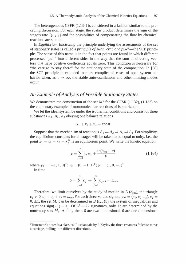
1.5. A Thermodynamic Analysis of the Chemical Kinetics Equations 97
The heterogeneous CSFR (1.134) is considered in a fashion similar to the pre-ceding discussion. For each stage, the scalar product determines the sign of thestage’s rate {γ, μx } and the possibilities of compensating the flow by chemicalreactions are studied.
In Equilibrium Encircling the principle underlying the assessments of the setof stationary states is called a principle of swan, crab and pike∗—the SCP princi-ple. The sense of this name is in the fact that points are found in which differentprocesses “pull” into different sides in the way that the sum of directing vec-tors that have positive coefficients equals zero. This condition is necessary for“the carrige to stay there” for the stationary state of the composition. In [58]the SCP principle is extended to more complicated cases of open system be-havior when, as τ → ∞, the stable auto-oscillations and other limiting modesoccur.
An Example of Analysis of Possible Stationary StatesWe demonstrate the construction of the set M0 for the CFSR (1.132), (1.133) onthe elementary example of monomolecular reactions of isomerization.
We let the ideal system be under the isothermal conditions and consist of threesubstances A1, A2, A3 obeying one balance relations
x1 + x2 + x3 = const.
Suppose that the mechanism of reaction is A1 � A2 � A3 � A1. For simplicity,the equilibrium constants for all stages will be taken to be equal to unity, i.e., thepoint x1 = x2 = x3 = xeq
j is an equilibrium point. We write the kinetic equation
c =3∑
s=1γsws + υ (cent − c)
V, (1.164)
where γ1 = (−1, 1, 0)T ; γ2 = (0, −1, 1)T ; γ3 = (1, 0, −1)T .In time
b =3∑
j=1c j →
3∑j=1
c jent = bent.
Therefore, we limit ourselves by the study of motion in D (bent), the trianglec j > 0, c1 + c2 + c3 = bent. For each three-valued signature ε = (ε1, ε2, ε3), ε j =0, ±1, the set Mε can be determined in D (bent)by the system of inequalities andequations sign(w j ) = ε j . Of 33 = 27 signatures, only 13 are determined by thenonempty sets Mε. Among them 6 are two-dimensional, 6 are one-dimensional
∗Transtator’s note: In a classical Russian tale by I. Krylov the three creatures failed to movea carriage, pulling it in different directions.
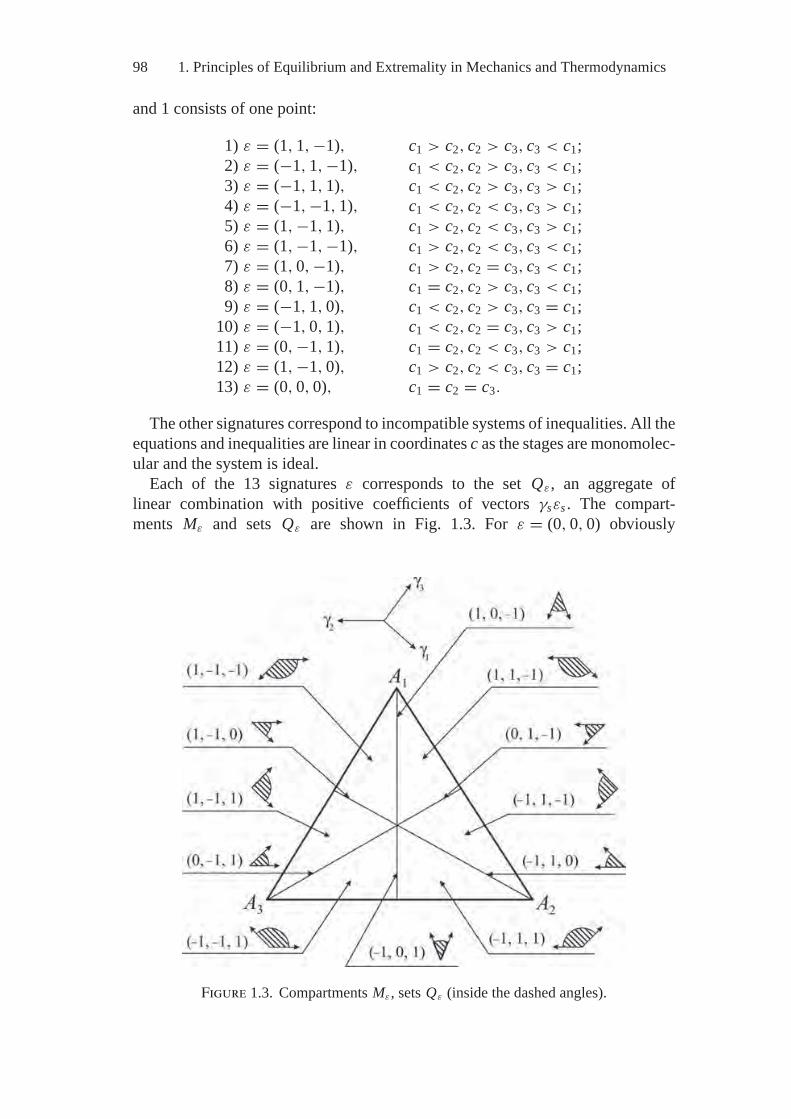
98 1. Principles of Equilibrium and Extremality in Mechanics and Thermodynamics
and 1 consists of one point:
1) ε = (1, 1, −1), c1 > c2, c2 > c3, c3 < c1;2) ε = (−1, 1, −1), c1 < c2, c2 > c3, c3 < c1;3) ε = (−1, 1, 1), c1 < c2, c2 > c3, c3 > c1;4) ε = (−1, −1, 1), c1 < c2, c2 < c3, c3 > c1;5) ε = (1, −1, 1), c1 > c2, c2 < c3, c3 > c1;6) ε = (1, −1, −1), c1 > c2, c2 < c3, c3 < c1;7) ε = (1, 0, −1), c1 > c2, c2 = c3, c3 < c1;8) ε = (0, 1, −1), c1 = c2, c2 > c3, c3 < c1;9) ε = (−1, 1, 0), c1 < c2, c2 > c3, c3 = c1;
10) ε = (−1, 0, 1), c1 < c2, c2 = c3, c3 > c1;11) ε = (0, −1, 1), c1 = c2, c2 < c3, c3 > c1;12) ε = (1, −1, 0), c1 > c2, c2 < c3, c3 = c1;13) ε = (0, 0, 0), c1 = c2 = c3.
The other signatures correspond to incompatible systems of inequalities. All theequations and inequalities are linear in coordinates c as the stages are monomolec-ular and the system is ideal.
Each of the 13 signatures ε corresponds to the set Qε, an aggregate oflinear combination with positive coefficients of vectors γsεs . The compart-ments Mε and sets Qε are shown in Fig. 1.3. For ε = (0, 0, 0) obviously
Figure 1.3. Compartments Mε , sets Qε (inside the dashed angles).
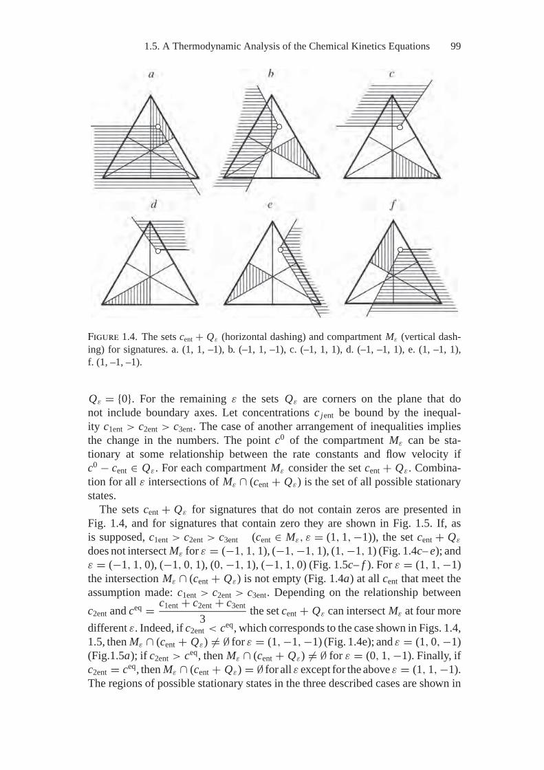
1.5. A Thermodynamic Analysis of the Chemical Kinetics Equations 99
Figure 1.4. The sets cent + Qε (horizontal dashing) and compartment Mε (vertical dash-ing) for signatures. a. (1, 1, –1), b. (–1, 1, –1), c. (–1, 1, 1), d. (–1, –1, 1), e. (1, –1, 1),f. (1, –1, –1).
Qε = {0}. For the remaining ε the sets Qε are corners on the plane that donot include boundary axes. Let concentrations c jent be bound by the inequal-ity c1ent > c2ent > c3ent. The case of another arrangement of inequalities impliesthe change in the numbers. The point c0 of the compartment Mε can be sta-tionary at some relationship between the rate constants and flow velocity ifc0 − cent ∈ Qε. For each compartment Mε consider the set cent + Qε. Combina-tion for all ε intersections of Mε ∩ (cent + Qε) is the set of all possible stationarystates.
The sets cent + Qε for signatures that do not contain zeros are presented inFig. 1.4, and for signatures that contain zero they are shown in Fig. 1.5. If, asis supposed, c1ent > c2ent > c3ent (cent ∈ Mε, ε = (1, 1, −1)), the set cent + Qε
does not intersect Mε for ε = (−1, 1, 1), (−1, −1, 1), (1, −1, 1) (Fig. 1.4c– e); andε = (−1, 1, 0), (−1, 0, 1), (0, −1, 1), (−1, 1, 0) (Fig. 1.5c– f ). For ε = (1, 1, −1)the intersection Mε ∩ (cent + Qε) is not empty (Fig. 1.4a) at all cent that meet theassumption made: c1ent > c2ent > c3ent. Depending on the relationship betweenc2ent and ceq = c1ent + c2ent + c3ent
3 the set cent + Qε can intersect Mε at four moredifferent ε. Indeed, if c2ent < ceq, which corresponds to the case shown in Figs. 1.4,1.5, then Mε ∩ (cent + Qε) �= ∅ for ε = (1, −1, −1) (Fig. 1.4e); and ε = (1, 0, −1)(Fig.1.5a); if c2ent > ceq, then Mε ∩ (cent + Qε) �= ∅ for ε = (0, 1, −1). Finally, ifc2ent = ceq, then Mε ∩ (cent + Qε) = ∅ for all ε except for the above ε = (1, 1, −1).The regions of possible stationary states in the three described cases are shown in
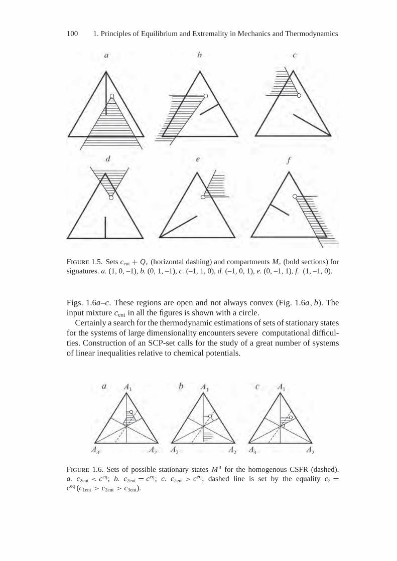
100 1. Principles of Equilibrium and Extremality in Mechanics and Thermodynamics
Figure 1.5. Sets cent + Qε (horizontal dashing) and compartments Mε (bold sections) forsignatures. a. (1, 0, –1), b. (0, 1, –1), c. (–1, 1, 0), d. (–1, 0, 1), e. (0, –1, 1), f. (1, –1, 0).
Figs. 1.6a–c. These regions are open and not always convex (Fig. 1.6a, b). Theinput mixture cent in all the figures is shown with a circle.
Certainly a search for the thermodynamic estimations of sets of stationary statesfor the systems of large dimensionality encounters severe computational difficul-ties. Construction of an SCP-set calls for the study of a great number of systemsof linear inequalities relative to chemical potentials.
1
23 3 2
1 1
3 2
Figure 1.6. Sets of possible stationary states M0 for the homogenous CSFR (dashed).a. c2ent < ceq; b. c2ent = ceq; c. c2ent > ceq; dashed line is set by the equality c2 =ceq (c1ent > c2ent > c3ent).
1.5. A Thermodynamic Analysis of the Chemical Kinetics Equations 101
To conclude this section we would like to note, that since the 1960s thermo-dynamic analysis of open system kinetics—with its main points briefly discussedin the sixth chapter of Equilibrium Encircling—has been developing in the worksof a number of the authors: F. Horn [47, 71], M. Feinberg [44, 45, 46, 47], P. M.Bowen [24], B. D. Coleman [29], D. Glasser [57, 70], D. D. Hildebrant [46, 57, 70],J. C. Keck [98], and V. N. Parmon [136] et al.
2Extreme Thermodynamic Models inTerms of Mathematical Programming
Physicists are too bad at mathematics to deal with physics.Einstein discovered the general relativity theory owing to his poor knowledge of thenon-Euclidean geometry.
D. Hilbert
2.1. Brief Information from Mathematical Programming
Before discussing the extreme models of equilibrium thermodynamics let us ad-dress the general statements of problems in mathematical programming (MP)that are used for construction of these models. The theory and methods of MPare presented in detail in numerous publications, for example [19, 33, 94, 142].In this chapter we present the minimum necessary information on linear, con-vex, and concave programming needed for understanding the further text of thebook.
The general problem of mathematical programming is formulated as follows:Find maximum (minimum) of the objective function f (x) provided that the vectorx = (x1, . . . , xn)T belongs to the admissible region D ⊂ Rn , where Rn is an n-dimensional Euclidean space. The vector xmax is called a global maximum pointof an objective function if
f(xmax) ≥ f (x) . (2.1)
The vector xmax is called a local maximum point of the objective function ifthere is an ε-vicinity
Uε =⎧⎨⎩x :
⎡⎣∥∥xmax − x
∥∥ =(
n∑j=1
(xmax
j − x j)2)0.5
⎤⎦ < ε
⎫⎬⎭ (2.2)
such that f (xmax) ≥ f (x) for all x ∈ Uε Similarly the points of global and localminima are found.
102
2.1. Brief Information from Mathematical Programming 103
According to the Weierstrass theorem the continuous function f (x) determinedon a closed limited admissible set D reaches the global maximum (minimum) onthe internal or boundary point of D.
To analyze the MP problems the notions of convexity and concavity of setsand functions are rather important. The set D ⊂ Rn is convex if from x1 ∈ D andx2 ∈ D at any λ (0 ≤ λ ≤ 1), it follows that
λx1 + (1 − λ) x2 ∈ D. (2.3)
This means that if any two points belong to a convex set the whole section con-necting them belongs to this set.
The function f (x) is called convex if at any x1 and x2 and 0 ≤ λ ≤ 1.
f (λx1 + (1 − λ) x2) ≤ λ f (x1) + (1 − λ) f (x2) , (2.4)
and concave, if
f (λx1 + (1 − λ) x2) ≥ λ f (x1) + (1 − λ) f (x2) . (2.5)
The sign of equality in (2.4) and (2.5) is true only for linear functions. At satisfiedstrict inequalities the functions are called strictly convex (2.4) and strictly concave(2.5).
The condition of strict convexity f (x) is positive definiteness of the matrix ofsecond derivatives (the Hessian matrix)
H (x) ={
∂2 f∂xi∂x j
}, i = 1, . . . , m, j = 1, . . . , n.
The symmetrical nonsingular (with a determinant distinct from zero) matrix ispositive definite if it is subject to the condition
xT Hx > 0, x ∈ Rn. (2.6)
Nonnegative definiteness (xT Hx ≥ 0) is indicative of function convexity.If f (x) is convex not on the whole space Rn but only on the polyhedron Ax = b,
x ≥ 0, the inequality (2.6) is supplemented by the condition Ax = 0.When the determinant (Hessian) H (x) equals zero, we have the most compli-
cated situation for determining wheter a function is convex or concave. Here theproperty of nonnegative definite matrices can be used; the property consists ofthe fact that the eigenvalues and principal minors of the matrix are nonnegativenumbers1 (for nonpositive definite matrices these numbers are nonpositive). Tobe sure, in the present book we do not have the opportunity to present the mainprinciples of matrix analysis in detail, and, therefore, give the references to thespecial literature [53, 72].
1 The number λ and nonzero vector x are called the eigenvalue and eigenvector of matrixA, respectively, if they satisfy the equation Ax = λx , which is equivalent to the equation(λI − A) x = 0. Where I is a singular matrix.
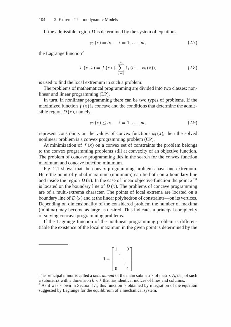
104 2. Extreme Thermodynamic Models
If the admissible region D is determined by the system of equations
ϕi (x) = bi , i = 1, . . . , m, (2.7)
the Lagrange function2
L (x, λ) = f (x) +m∑
i=1λi (bi − ϕi (x)), (2.8)
is used to find the local extremum in such a problem.The problems of mathematical programming are divided into two classes: non-
linear and linear programming (LP).In turn, in nonlinear programming there can be two types of problems. If the
maximized function f (x) is concave and the conditions that determine the admis-sible region D (x), namely,
ϕi (x) ≤ bi , i = 1, . . . , m, (2.9)
represent constraints on the values of convex functions ϕi (x), then the solvednonlinear problem is a convex programming problem (CP).
At minimization of f (x) on a convex set of constraints the problem belongsto the convex programming problems still at convexity of an objective function.The problem of concave programming lies in the search for the convex functionmaximum and concave function minimum.
Fig. 2.1 shows that the convex programming problems have one extremum.Here the point of global maximum (minimum) can lie both on a boundary lineand inside the region D (x). In the case of linear objective function the point xext
is located on the boundary line of D (x). The problems of concave programmingare of a multi-extrema character. The points of local extrema are located on aboundary line of D (x) and at the linear polyhedron of constraints—on its vertices.Depending on dimensionality of the considered problem the number of maxima(minima) may become as large as desired. This indicates a principal complexityof solving concave programming problems.
If the Lagrange function of the nonlinear programming problem is differen-tiable the existence of the local maximum in the given point is determined by the
I =
⎡⎢⎢⎢⎣
1 0···
0 1
⎤⎥⎥⎥⎦
The principal minor is called a determinant of the main submatrix of matrix A, i.e., of sucha submatrix with a dimension k × k that has identical indices of lines and columns.2 As it was shown in Section 1.1, this function is obtained by integration of the equationsuggested by Lagrange for the equilibrium of a mechanical system.
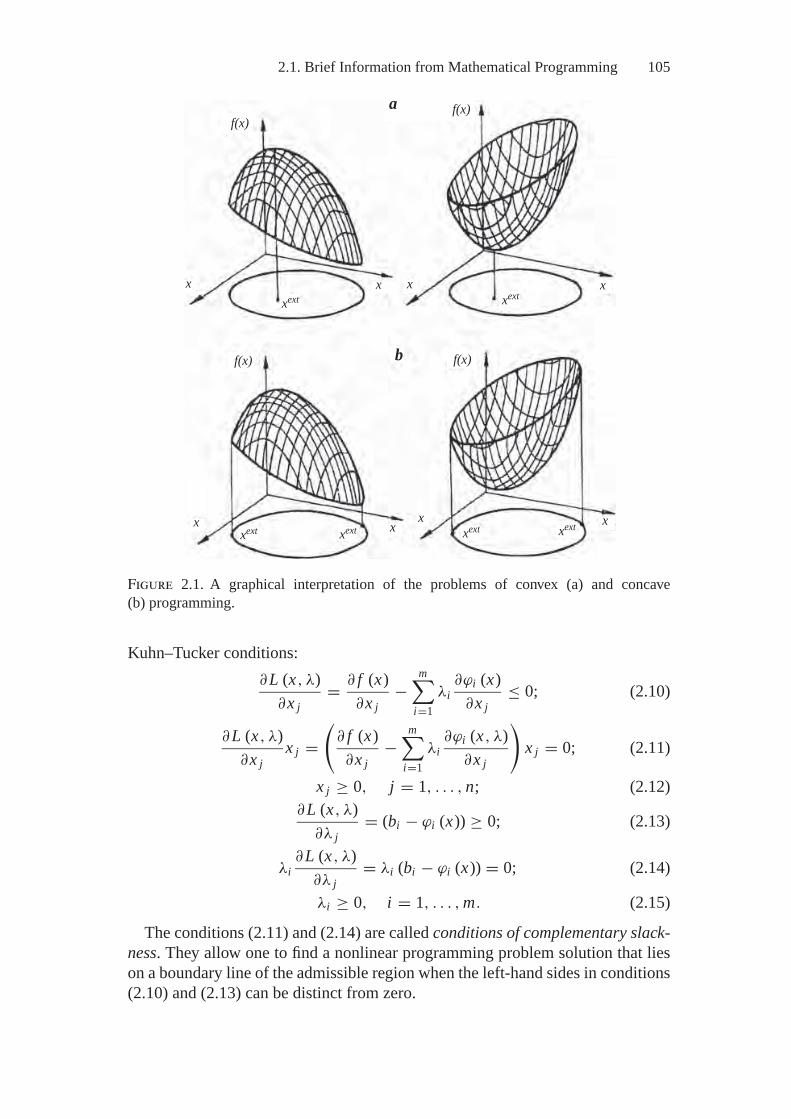
2.1. Brief Information from Mathematical Programming 105
f(x)
f(x) f(x)
f(x)
x
x
x
x
x
x
x
x
xext xext
xextxextxext xext
a
b
Figure 2.1. A graphical interpretation of the problems of convex (a) and concave(b) programming.
Kuhn–Tucker conditions:∂L (x, λ)
∂x j= ∂ f (x)
∂x j−
m∑i=1
λi∂ϕi (x)
∂x j≤ 0; (2.10)
∂L (x, λ)∂x j
x j =(
∂ f (x)∂x j
−m∑
i=1λi
∂ϕi (x, λ)∂x j
)x j = 0; (2.11)
x j ≥ 0, j = 1, . . . , n; (2.12)∂L (x, λ)
∂λ j= (bi − ϕi (x)) ≥ 0; (2.13)
λi∂L (x, λ)
∂λ j= λi (bi − ϕi (x)) = 0; (2.14)
λi ≥ 0, i = 1, . . . , m. (2.15)
The conditions (2.11) and (2.14) are called conditions of complementary slack-ness. They allow one to find a nonlinear programming problem solution that lieson a boundary line of the admissible region when the left-hand sides in conditions(2.10) and (2.13) can be distinct from zero.
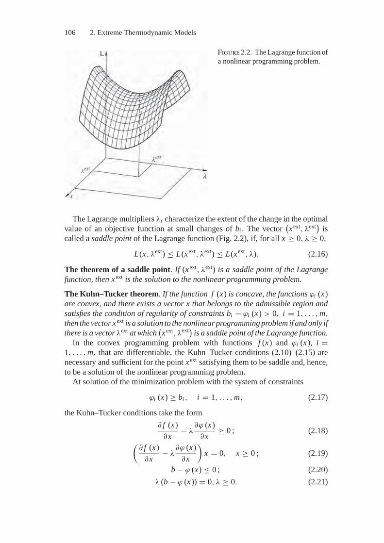
106 2. Extreme Thermodynamic Models
Figure 2.2. The Lagrange function ofa nonlinear programming problem.
The Lagrange multipliers λi characterize the extent of the change in the optimalvalue of an objective function at small changes of bi . The vector
(xext, λext) is
called a saddle point of the Lagrange function (Fig. 2.2), if, for all x ≥ 0, λ ≥ 0,
L(x, λext) ≤ L(xext, λext) ≤ L(xext, λ). (2.16)
The theorem of a saddle point. If (xext, λext) is a saddle point of the Lagrangefunction, then xext is the solution to the nonlinear programming problem.
The Kuhn–Tucker theorem. If the function f (x) is concave, the functions ϕi (x)are convex, and there exists a vector x that belongs to the admissible region andsatisfies the condition of regularity of constraints bi − ϕi (x) > 0, i = 1, . . . , m,then the vector xext is a solution to the nonlinear programming problem if and only ifthere is a vector λext at which
(xext, λext) is a saddle point of the Lagrange function.
In the convex programming problem with functions f (x) and ϕi (x), i =1, . . . , m, that are differentiable, the Kuhn–Tucker conditions (2.10)–(2.15) arenecessary and sufficient for the point xext satisfying them to be saddle and, hence,to be a solution of the nonlinear programming problem.
At solution of the minimization problem with the system of constraints
ϕi (x) ≥ bi , i = 1, . . . , m, (2.17)
the Kuhn–Tucker conditions take the form∂ f (x)
∂x− λ
∂ϕ (x)∂x
≥ 0 ; (2.18)(∂ f (x)
∂x− λ
∂ϕ (x)∂x
)x = 0, x ≥ 0 ; (2.19)
b − ϕ (x) ≤ 0 ; (2.20)λ (b − ϕ (x)) = 0, λ ≥ 0. (2.21)
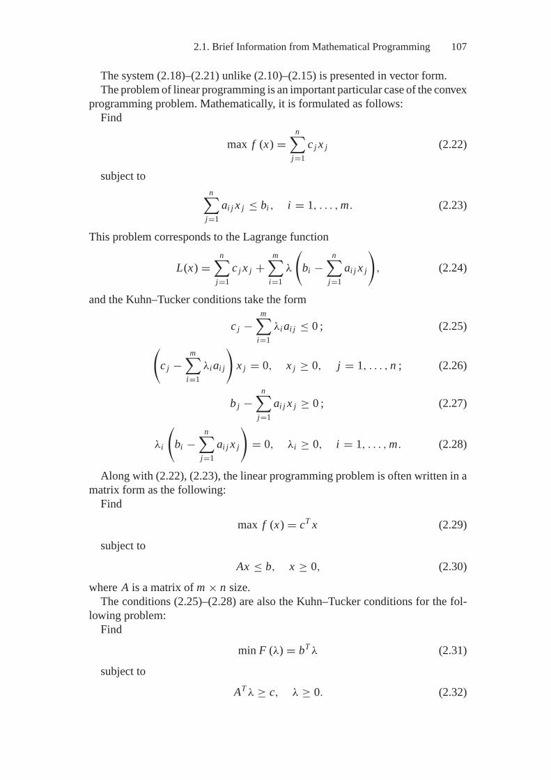
2.1. Brief Information from Mathematical Programming 107
The system (2.18)–(2.21) unlike (2.10)–(2.15) is presented in vector form.The problem of linear programming is an important particular case of the convex
programming problem. Mathematically, it is formulated as follows:Find
max f (x) =n∑
j=1c j x j (2.22)
subject ton∑
j=1ai j x j ≤ bi , i = 1, . . . , m. (2.23)
This problem corresponds to the Lagrange function
L(x) =n∑
j=1c j x j +
m∑i=1
λ
(bi −
n∑j=1
ai j x j
), (2.24)
and the Kuhn–Tucker conditions take the form
c j −m∑
i=1λi ai j ≤ 0 ; (2.25)
(c j −
m∑i=1
λi ai j
)x j = 0, x j ≥ 0, j = 1, . . . , n ; (2.26)
b j −n∑
j=1ai j x j ≥ 0 ; (2.27)
λi
(bi −
n∑j=1
ai j x j
)= 0, λi ≥ 0, i = 1, . . . , m. (2.28)
Along with (2.22), (2.23), the linear programming problem is often written in amatrix form as the following:
Find
max f (x) = cT x (2.29)
subject to
Ax ≤ b, x ≥ 0, (2.30)
where A is a matrix of m × n size.The conditions (2.25)–(2.28) are also the Kuhn–Tucker conditions for the fol-
lowing problem:Find
min F (λ) = bT λ (2.31)
subject to
AT λ ≥ c, λ ≥ 0. (2.32)
108 2. Extreme Thermodynamic Models
This minimization problem is called “dual” with respect to the direct maxi-mization problem (2.22), (2.23) or (2.29), (2.30). The constraints (2.23) of thedirect problem correspond to the variables λi (the Lagrange multipliers) of thedual problem and vice-versa.
Each constraint-inequality of the direct problem corresponds to part of the spaceRn , and this part is limited by the plane
n∑j=1
ai j x j = b j (2.33)
or x j = 0. Intersection of such half-spaces forms a convex admissible region D (x),i.e., a polyhedron of constraints. Similarly the admissible region of solutions to adual problem D(λ) is formed. The vertices of the polyhedron are the interceptionpoints of the planes. The solution xext of the linear programming problem alwayscoincides with one of the polyhedron vertices (in the case of degeneracy with anface) (Fig.2.3). This solution satisfies the duality theorem.
The duality theorem. The admissible vector is a solution to the linear program-ming problem if and only if there exists such an admissible vector λ of the dualproblem that the values of the objective functions on these vectors are equal (i.e.,f (x) = F (λ)). Here the vector λ is the dual problem solution.
When we set the constraints of the linear programming problem in the form ofequalities the number of components of the vector xext always equals m, i.e.,the number of constraints. If some of these components turn out to be equalto zero the solution of the direct problem is degenerate and the solution of thedual one is many-valued (a set of solutions is some face of the polyhedron ofconstraints).
To solve the linear programming problem a number of methods were devel-oped including the most widely used simplex method [33] that was employed innumerous standard programs for computers.
Figure 2.3. A graphical interpretation of the linear programming problem.
2.2. The Model of Extreme Intermediate States (MEIS) 109
Along with convex, concave, and linear problems the book gives also consid-eration to the parametric programming problems. In the parametric programmingthe objective function value depends on both the variables x and parameter y. Forthe latter, a range of potential values is set. The extremum f (x, y) is sought foreach fixed value y among which we find yext.
2.2. The Model of Extreme Intermediate States (MEIS)
Description of Final Complete EquilibriaLet us analyze the models that represent the entire thermodynamic attainabilityregion Dt of a physical-chemical system and start the analysis with the descriptionof final (complete) equilibrium xeq in terms of mathematical programming. Firstof all, the point xeq corresponds to the global extremum of characteristic thermo-dynamic function on Dt and to a certain extent can serve as a reference point forlocating the other equilibria in the attainability region. The model of xeq is certainlymuch simpler than the descriptions of the other points in Dt , and consideration ofits specific features must help one’s understanding of the properties of the modelsof Dt , on the whole.
All the mathematical statements of the problems in this section are given asapplied to constant T and P which is true for most of the technological andmany natural processes. The other conditions of systems’ interaction with theenvironment are considered in the next section.
For the conditions assumed here the problems of the search for xeq in terms ofMP takes the following form:
Find
min[
G (x) =∑
jG j (x) x j
]= G(xeq) (2.34)
subject to
Ax = b, (2.35)G j = f j (x) , (2.36)
x j ≥ 0, (2.37)
where G and G j are Gibbs energy of the system and a mole of its j th component,respectively; x = (x1, . . . , xn)T is a vector of mole quantities of components; A =[ai j ] is the m × n matrix of element contents in the components of the system;b = (b1, . . . , bm)T is a vector of mole quantities of elements; and the index i refersto the i th element.
The physical sense of the objective function (2.34) is obvious. The matrix equa-tion (2.35) determines the condition of conservation of the element amounts. Theform of the function (2.36) depends on the type of system under study (ideal gas,real gas, heterogeneous mixture, etc.).
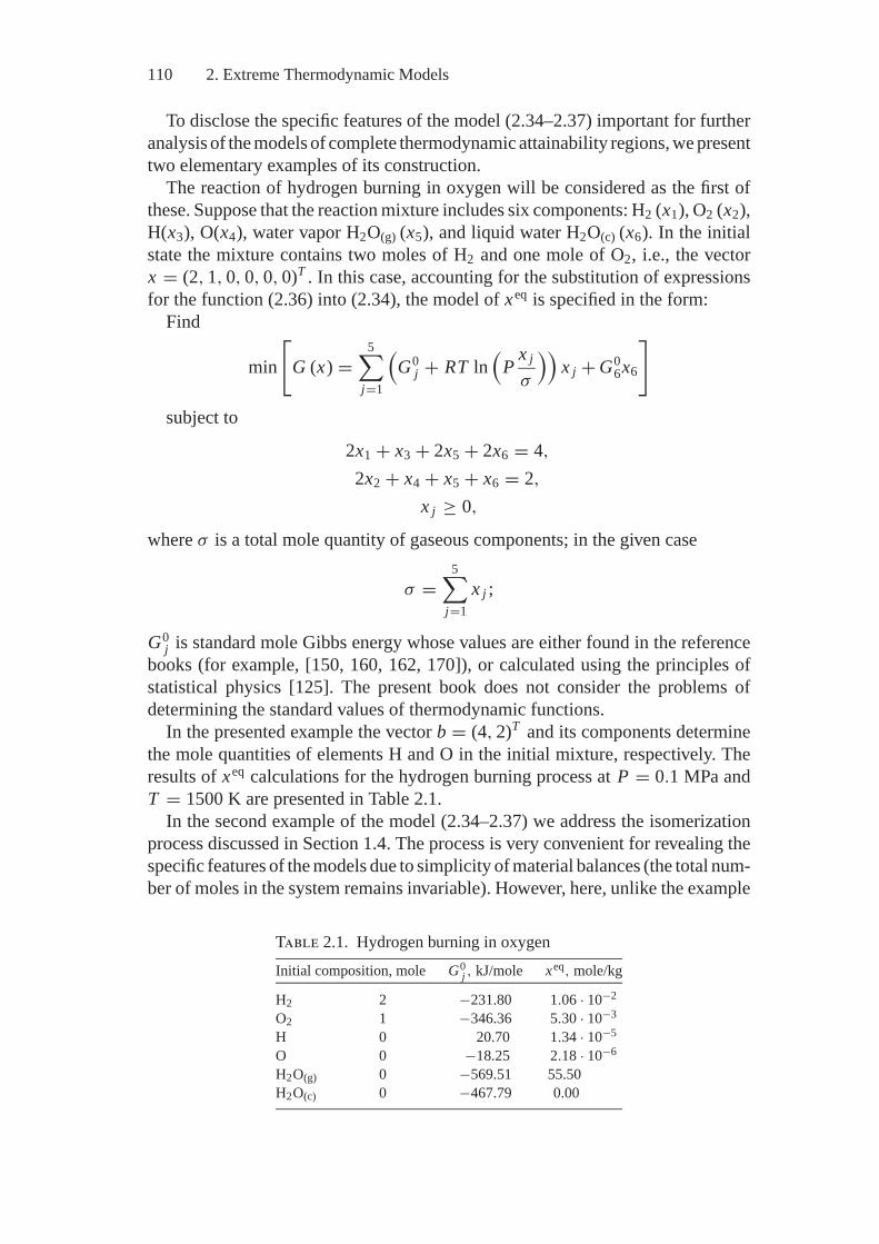
110 2. Extreme Thermodynamic Models
To disclose the specific features of the model (2.34–2.37) important for furtheranalysis of the models of complete thermodynamic attainability regions, we presenttwo elementary examples of its construction.
The reaction of hydrogen burning in oxygen will be considered as the first ofthese. Suppose that the reaction mixture includes six components: H2 (x1), O2 (x2),H(x3), O(x4), water vapor H2O(g) (x5), and liquid water H2O(c) (x6). In the initialstate the mixture contains two moles of H2 and one mole of O2, i.e., the vectorx = (2, 1, 0, 0, 0, 0)T . In this case, accounting for the substitution of expressionsfor the function (2.36) into (2.34), the model of xeq is specified in the form:
Find
min[
G (x) =5∑
j=1
(G0
j + RT ln(
Px j
σ
))x j + G0
6x6
]
subject to
2x1 + x3 + 2x5 + 2x6 = 4,
2x2 + x4 + x5 + x6 = 2,
x j ≥ 0,
where σ is a total mole quantity of gaseous components; in the given case
σ =5∑
j=1x j ;
G0j is standard mole Gibbs energy whose values are either found in the reference
books (for example, [150, 160, 162, 170]), or calculated using the principles ofstatistical physics [125]. The present book does not consider the problems ofdetermining the standard values of thermodynamic functions.
In the presented example the vector b = (4, 2)T and its components determinethe mole quantities of elements H and O in the initial mixture, respectively. Theresults of xeq calculations for the hydrogen burning process at P = 0.1 MPa andT = 1500 K are presented in Table 2.1.
In the second example of the model (2.34–2.37) we address the isomerizationprocess discussed in Section 1.4. The process is very convenient for revealing thespecific features of the models due to simplicity of material balances (the total num-ber of moles in the system remains invariable). However, here, unlike the example
Table 2.1. Hydrogen burning in oxygenInitial composition, mole G0
j , kJ/mole xeq, mole/kg
H2 2 −231.80 1.06 · 10−2
O2 1 −346.36 5.30 · 10−3
H 0 20.70 1.34 · 10−5
O 0 −18.25 2.18 · 10−6
H2O(g) 0 −569.51 55.50H2O(c) 0 −467.79 0.00
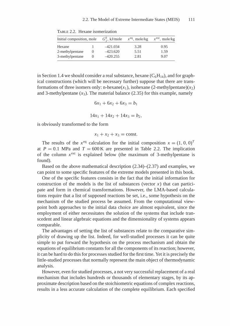
2.2. The Model of Extreme Intermediate States (MEIS) 111
Table 2.2. Hexane isomerizationInitial composition, mole G0
j , kJ/mole xeq, mole/kg xext, mole/kg
Hexane 1 –421.034 3.28 0.952-methylpentane 0 –423.620 5.51 1.593-methylpentane 0 –420.255 2.81 9.07
in Section 1.4 we should consider a real substance, hexane (C6H14), and for graph-ical constructions (which will be necessary further) suppose that there are trans-formations of three isomers only: n-hexane(x1), isohexane (2-methylpentane)(x2)and 3-methylpentane (x3). The material balance (2.35) for this example, namely
6x1 + 6x2 + 6x3 = b1
14x1 + 14x2 + 14x3 = b2,
is obviously transformed to the form
x1 + x2 + x3 = const.
The results of the xeq calculation for the initial composition x = (1, 0, 0)T
at P = 0.1 MPa and T = 600 K are presented in Table 2.2. The implicationof the column xext is explained below (the maximum of 3-methylpentane isfound).
Based on the above mathematical description (2.34)–(2.37) and examples, wecan point to some specific features of the extreme models presented in this book.
One of the specific features consists in the fact that the initial information forconstruction of the models is the list of substances (vector x) that can partici-pate and form in chemical transformations. However, the LMA-based calcula-tions require that a list of supposed reactions be set, i.e., some hypothesis on themechanism of the studied process be assumed. From the computational view-point both approaches to the initial data choice are almost equivalent, since theemployment of either necessitates the solution of the systems that include tran-scedent and linear algebraic equations and the dimensionality of systems appearscomparable.
The advantages of setting the list of substances relate to the comparative sim-plicity of drawing up the list. Indeed, for well-studied processes it can be quitesimple to put forward the hypothesis on the process mechanism and obtain theequations of equilibrium constants for all the components of its reaction; however,it can be hard to do this for processes studied for the first time. Yet it is precisely thelittle-studied processes that normally represent the main object of thermodynamicanalysis.
However, even for studied processes, a not very successful replacement of a realmechanism that includes hundreds or thousands of elementary stages, by its ap-proximate description based on the stoichiometric equations of complex reactions,results in a less accurate calculation of the complete equilibrium. Each specified
112 2. Extreme Thermodynamic Models
list of reactions corresponds to its partial equilibrium satisfying the condition thatthe reactions absented from this list do not take place in the reacting system. Thisequilibrium does not coincide with the complete one.
To some extent the problem of the initial data preparation using LMA can besolved if, as in the case of applying the model (2.34)–(2.37), we make a list ofsupposed components of the reaction mixture and then write for each of themthe reaction of its synthesis from elements. Such a replacement of the list ofstages, that is, the actual mechanism of the process, by the synthesis reactionsis admissible, since the state xeq at a given vector b and conditions of interac-tion with the environment do not depend on the initial composition of reagents.However, here, in the case of modeling complex multicomponent and multi-phase systems, difficulties in searching analytical solution to the problem mayappear.
It should be emphasized that the extreme approach as compared to LMA doesnot impose strict limitations on the method of setting the initial information andallows its representation in the form of both the list of substances and the list ofreactions. The model based on the latter method of initial data representation isconsidered at the end of this section.
Commenting on the model (2.34)–(2.37) let us focus once again on the fact (seeSection I.17) that at its description (as in the later description of other extrememodels) the notion of “component” has not been interpreted in the way that ithas generally been in the thermodynamic literature, starting, apparently, with thebook by Gibbs, On Equilibrium of Heterogeneous Substances. By “components”in thermodynamics, writers on the subject usually mean the substances of thereaction mixture, disregarding the number of phases in which they are present.In this book any single phase of a substance is considered to be an individualcomponent. For instance, in the first of the above examples, water is representedby two components of the vector x : gaseous (x5) and liquid (x6). Such a breakwith the tradition makes easier the construction of mathematical models. Indeed,when calculating equilibria we always need to find the amount of each substance ineach phase and, therefore, it is natural to consider these quantities as independentvariables of the problem. Below, it will be shown that the assumed principle offorming the composition of variables allows one to overcome some computationaldifficulties in the search for equilibrium states.
The Model of Extreme Intermediate States (MEIS)Now let us discuss the main thermodynamic model used by the authors, the modelof extreme intermediate states (MEIS). For a fixed T, P , and initial compositionof reagents y, MEIS has the following form:
Find
max(
F(x) =∑j∈J ext
c j x j
)= F(xext) (2.38)
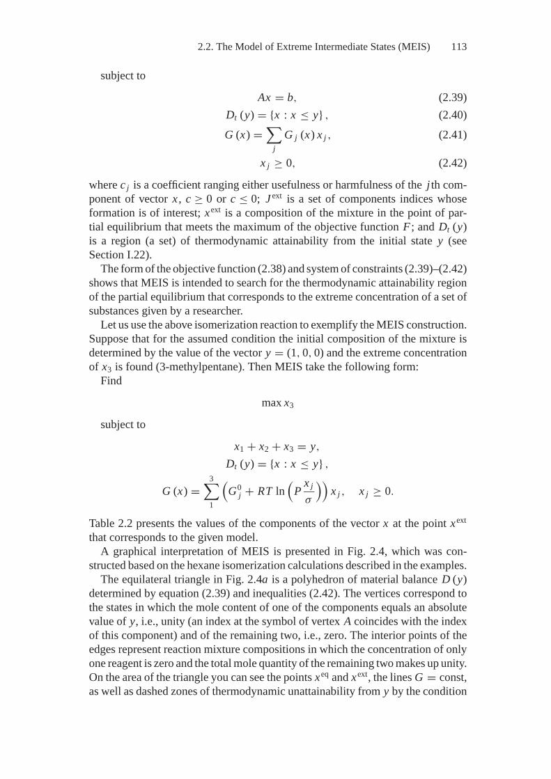
2.2. The Model of Extreme Intermediate States (MEIS) 113
subject to
Ax = b, (2.39)Dt (y) = {x : x ≤ y} , (2.40)G (x) =
∑j
G j (x) x j , (2.41)
x j ≥ 0, (2.42)
where c j is a coefficient ranging either usefulness or harmfulness of the j th com-ponent of vector x , c ≥ 0 or c ≤ 0; J ext is a set of components indices whoseformation is of interest; xext is a composition of the mixture in the point of par-tial equilibrium that meets the maximum of the objective function F ; and Dt (y)is a region (a set) of thermodynamic attainability from the initial state y (seeSection I.22).
The form of the objective function (2.38) and system of constraints (2.39)–(2.42)shows that MEIS is intended to search for the thermodynamic attainability regionof the partial equilibrium that corresponds to the extreme concentration of a set ofsubstances given by a researcher.
Let us use the above isomerization reaction to exemplify the MEIS construction.Suppose that for the assumed condition the initial composition of the mixture isdetermined by the value of the vector y = (1, 0, 0) and the extreme concentrationof x3 is found (3-methylpentane). Then MEIS take the following form:
Find
max x3
subject to
x1 + x2 + x3 = y,
Dt (y) = {x : x ≤ y} ,
G (x) =3∑1
(G0
j + RT ln(
Px j
σ
))x j , x j ≥ 0.
Table 2.2 presents the values of the components of the vector x at the point xext
that corresponds to the given model.A graphical interpretation of MEIS is presented in Fig. 2.4, which was con-
structed based on the hexane isomerization calculations described in the examples.The equilateral triangle in Fig. 2.4a is a polyhedron of material balance D (y)
determined by equation (2.39) and inequalities (2.42). The vertices correspond tothe states in which the mole content of one of the components equals an absolutevalue of y, i.e., unity (an index at the symbol of vertex A coincides with the indexof this component) and of the remaining two, i.e., zero. The interior points of theedges represent reaction mixture compositions in which the concentration of onlyone reagent is zero and the total mole quantity of the remaining two makes up unity.On the area of the triangle you can see the points xeq and xext, the lines G = const,as well as dashed zones of thermodynamic unattainability from y by the condition
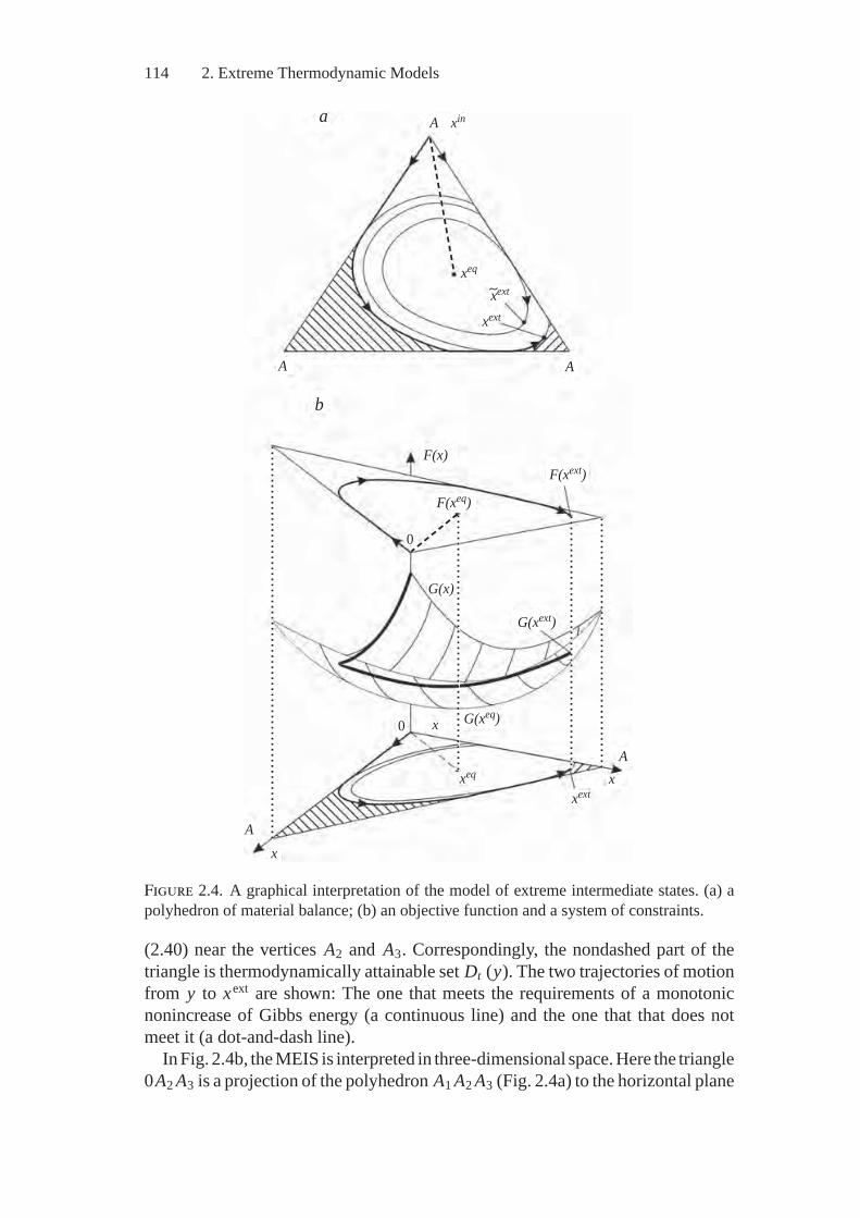
114 2. Extreme Thermodynamic Models
a
b
xeq
xext
xext
A A
A xin
F(x)
G(x)
F(xeq)
G(xeq)
F(xext)
G(xext)
xeq
xextx
x
x
A
A
0
0
Figure 2.4. A graphical interpretation of the model of extreme intermediate states. (a) apolyhedron of material balance; (b) an objective function and a system of constraints.
(2.40) near the vertices A2 and A3. Correspondingly, the nondashed part of thetriangle is thermodynamically attainable set Dt (y). The two trajectories of motionfrom y to xext are shown: The one that meets the requirements of a monotonicnonincrease of Gibbs energy (a continuous line) and the one that that does notmeet it (a dot-and-dash line).
In Fig. 2.4b, the MEIS is interpreted in three-dimensional space. Here the triangle0A2 A3 is a projection of the polyhedron A1 A2 A3 (Fig. 2.4a) to the horizontal plane
2.2. The Model of Extreme Intermediate States (MEIS) 115
x20x3 of a positive octant. Along the vertical axis the Gibbs energy values (in themiddle of the figure) and the objective function F(x) (on top) are plotted. The pointsxeq and xext, the lines G = const, and the admissible and inadmissible trajectoryof transition from y to xext are shown both on the plane of compositions (x20x3),on the surface G(x), and on the objective function plane.
Even based on the above short analysis, we can see the principal advantages ofMEIS as compared to the traditional models of final equilibria [9, 32, 96, 97, 172].
First, instead of searching for the single point xeq, the whole set Dt (y) canbe examined in the course of optimization. This allows many technological andnatural processes in which final equilibria that are not attained by the conditions ofkinetics to be included into the area of equilibrium thermodynamics applications.
Second, calculating the extreme values of the corresponding thermodynamicfunctions, we determine, depending on the purpose of the study, the extreme con-centrations of useful or harmful substances formed in the studied process. Thismakes the thermodynamic analysis more substantial.
Third, the models of type (2.38)–(2.42) are easily supplemented by variousconstraints in the form of equalities and inequalities that can be employed inthe thermodynamic analysis and make possible consideration for the impact ofnon-thermodynamic factors associated with the specific features of the system atissue: chemical kinetics; transfer processes (heat and mass transfer); and limitingvalues of parameters (if they are not fixed): temperature, pressure, concentrationsof individual components, energy input and output, etc.
Description of Nonthermodynamic ConstraintsLet us consider in more detail the last of the mentioned MEIS advantages. Onone hand, this advantage is caused by the capabilities of the MP that allow theproblem statements to be easily varied. On the other hand, it is due to the univer-sal character of thermodynamics, whose principles rule diverse physical-chemicalprocess. The examples of interpreting the stationary and nonstationary modelsof motion that differ in nature in terms of thermodynamics were already pre-sented in Section 1.3. In all the considered cases it was difficult to replace thedescriptions of change with time in the studied system’s state by the descrip-tion of the states of rest (equilibrium). Using as applied to MEIS the techniquesof replacing the descriptions similar to those mentioned above, we should keeptrack of the transformation correctness in relation to both the final and the partialequilibria.
A natural way of taking into account the factors that are traditionally considerednonthermodynamic, for example, the specific features of the transfer processes, isto change the form of the functions entering into conditions (2.40) and (2.41), toinclude in them—along with the chemical—the electrical, gravitational, or othercomponents related to the interactions that affect the transfer. Determination of thetype of generalized functions to be formed is exemplified in the final two chapter ofthis book, which is devoted to applications of the extreme thermodynamic models.Here, we first consider the possibility of taking into account various processes
116 2. Extreme Thermodynamic Models
running in a studied system by including additional constraints in the form ofequalities and inequalities into the model (2.38)–(2.42).
The constraint on the rate of oxygen diffusion to the surface of a substance beingoxidized can be presented in the form of inequality
xO2 ≥ xbO2
,
where xbO2
is the amount of O2 that, subject to mass exchange, cannot participatein reaction.
The constraint on the endothermic process of nitrogen oxide formation at fuelburning in the system with fixed P and T is described by the inequality
H ≤ Hb,
Where H is system enthalpy and Hb is fuel combustion heat. The latter inequalitycan be interpreted as a constraint on a potential range of technological regulationof the reaction mixture parameters. Meeting this constraint alone makes it possibleto maintain the given T and P .
MEIS can also include essentially more complicated expressions than the abovetwo inequalities. For example, if the mechanism of chemical transformations in-cludes the isomerization reactions
x1 → x2 → x3,
that meet the equationdx j
dτ= −k j x j ,
the integrals of kinetic equations
x1 = e−k1τ ,
x2 = k1
k2 − k1(e−k1τ − e−k2τ ),
x3 = 1 − k2
k2 − k1e−k1τ + k1
k2 − k1e−k2τ
can be used to make up the system of MEIS constraints.For example, we can write the constraint on the change in the amount of the
second component
x2 = k1
k2 − k1(e−k1τ − e−k2τ ), τ ≤ τ b,
in which the main variable of kinetics, time, is used as a parameter of “rest” states.Figure 2.5 shows that for the elementary system with only one isomerization
reaction x1 → x2 the curve of the kinetic equation x = f (τ ) is projected on thepolyhedron of material balance x1 + x2 = const, and, depending on the value of τ b
(a limiting time of the process), it limits the region of thermodynamic attainabilityfrom the initial state.
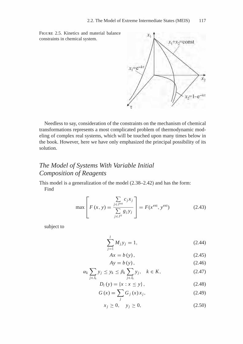
2.2. The Model of Extreme Intermediate States (MEIS) 117
Figure 2.5. Kinetics and material balanceconstraints in chemical system.
Needless to say, consideration of the constraints on the mechanism of chemicaltransformations represents a most complicated problem of thermodynamic mod-eling of complex real systems, which will be touched upon many times below inthe book. However, here we have only emphasized the principal possibility of itssolution.
The Model of Systems With Variable InitialComposition of ReagentsThis model is a generalization of the model (2.38–2.42) and has the form:
Find
max
⎡⎢⎣F (x, y) =
∑j∈J ext
c j x j∑j∈J 0
g j y j
⎤⎥⎦ = F(xext, yext) (2.43)
subject to
l∑j=1
M j y j = 1, (2.44)
Ax = b (y) , (2.45)Ay = b (y) , (2.46)
αk∑j∈Jk
y j ≤ yk ≤ βk∑j∈Jk
y j , k ∈ K , (2.47)
Dt (y) = {x : x ≤ y} , (2.48)G (x) =
∑j
G j (x) x j , (2.49)
x j ≥ 0, y j ≥ 0, (2.50)
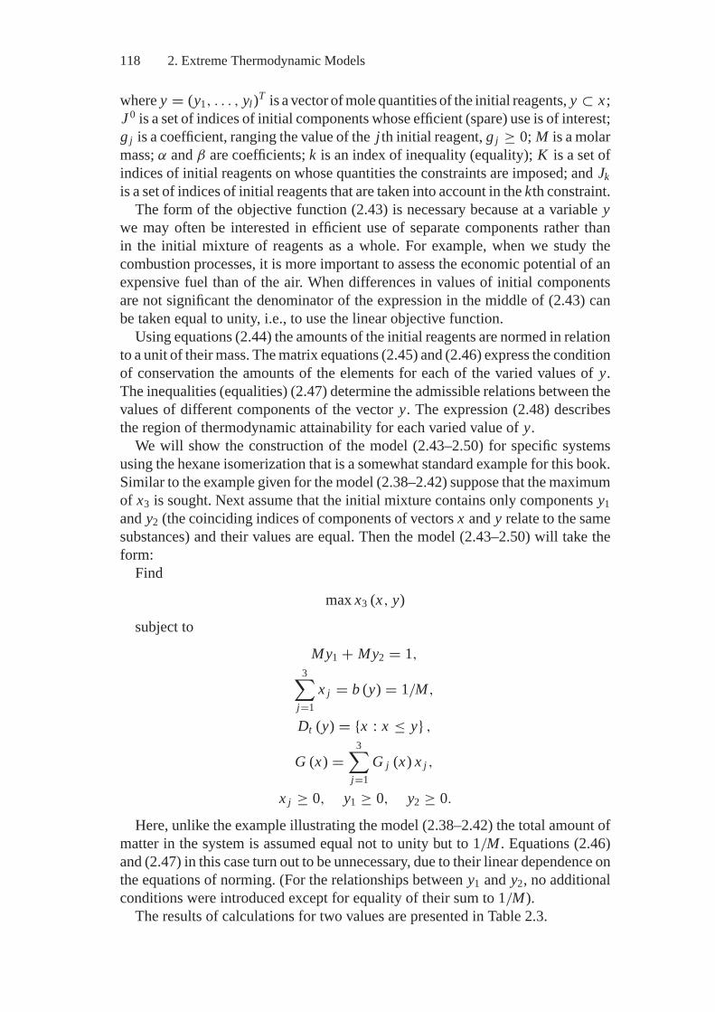
118 2. Extreme Thermodynamic Models
where y = (y1, . . . , yl)T is a vector of mole quantities of the initial reagents, y ⊂ x ;J 0 is a set of indices of initial components whose efficient (spare) use is of interest;g j is a coefficient, ranging the value of the j th initial reagent, g j ≥ 0; M is a molarmass; α and β are coefficients; k is an index of inequality (equality); K is a set ofindices of initial reagents on whose quantities the constraints are imposed; and Jkis a set of indices of initial reagents that are taken into account in the kth constraint.
The form of the objective function (2.43) is necessary because at a variable ywe may often be interested in efficient use of separate components rather thanin the initial mixture of reagents as a whole. For example, when we study thecombustion processes, it is more important to assess the economic potential of anexpensive fuel than of the air. When differences in values of initial componentsare not significant the denominator of the expression in the middle of (2.43) canbe taken equal to unity, i.e., to use the linear objective function.
Using equations (2.44) the amounts of the initial reagents are normed in relationto a unit of their mass. The matrix equations (2.45) and (2.46) express the conditionof conservation the amounts of the elements for each of the varied values of y.The inequalities (equalities) (2.47) determine the admissible relations between thevalues of different components of the vector y. The expression (2.48) describesthe region of thermodynamic attainability for each varied value of y.
We will show the construction of the model (2.43–2.50) for specific systemsusing the hexane isomerization that is a somewhat standard example for this book.Similar to the example given for the model (2.38–2.42) suppose that the maximumof x3 is sought. Next assume that the initial mixture contains only components y1and y2 (the coinciding indices of components of vectors x and y relate to the samesubstances) and their values are equal. Then the model (2.43–2.50) will take theform:
Findmax x3 (x, y)
subject toMy1 + My2 = 1,
3∑j=1
x j = b (y) = 1/M,
Dt (y) = {x : x ≤ y} ,
G (x) =3∑
j=1G j (x) x j ,
x j ≥ 0, y1 ≥ 0, y2 ≥ 0.
Here, unlike the example illustrating the model (2.38–2.42) the total amount ofmatter in the system is assumed equal not to unity but to 1/M . Equations (2.46)and (2.47) in this case turn out to be unnecessary, due to their linear dependence onthe equations of norming. (For the relationships between y1 and y2, no additionalconditions were introduced except for equality of their sum to 1/M).
The results of calculations for two values are presented in Table 2.3.
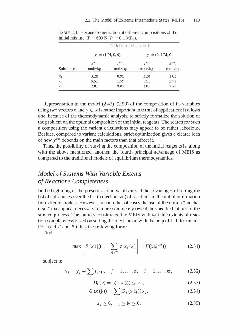
2.2. The Model of Extreme Intermediate States (MEIS) 119
Table 2.3. Hexane isomerization at different compositions of theinitial mixture (T = 600 K, P = 0.1 MPa).
Initial composition, mole
y = (1/M, 0, 0) y = (0, 1/M, 0)
xeq, xext, xeq, xext,Substance mole/kg mole/kg mole/kg mole/kg
x1 3.28 0.95 3.28 1.62x2 5.51 1.59 5.51 2.71x3 2.81 9.07 2.81 7.28
Representation in the model (2.43)–(2.50) of the composition of its variablesusing two vectors x and y ⊂ x is rather important in terms of application: It allowsone, because of the thermodynamic analysis, to strictly formalize the solution ofthe problem on the optimal composition of the initial reagents. The search for sucha composition using the variant calculations may appear to be rather laborious.Besides, compared to variant calculations, strict optimization gives a clearer ideaof how yext depends on the main factors than that affect it.
Thus, the possibility of varying the composition of the initial reagents is, alongwith the above mentioned, another, the fourth principal advantage of MEIS ascompared to the traditional models of equilibrium thermodynamics.
Model of Systems With Variable Extentsof Reactions CompletenessIn the beginning of the present section we discussed the advantages of setting thelist of substances over the list (a mechanism) of reactions in the initial informationfor extreme models. However, in a number of cases the use of the notion “mecha-nism” may appear necessary to more completely reveal the specific features of thestudied process. The authors constructed the MEIS with variable extents of reac-tion completeness based on setting the mechanism with the help of L. I. Rozonoer.For fixed T and P it has the following form:
Find
max[
F (x (ξ )) =∑j∈J ext
c j x j (ξ )]
= F(x(ξ ext)) (2.51)
subject to
x j = y j +∑
iνi jξi , j = 1, . . . , n, i = 1, . . . , m, (2.52)
Dt (y) = {ξ : x (ξ ) ≤ y} , (2.53)G (x (ξ )) =
∑j
G j (x (ξ )) x j , (2.54)
x j ≥ 0, 1 ≥ ξi ≥ 0, (2.55)
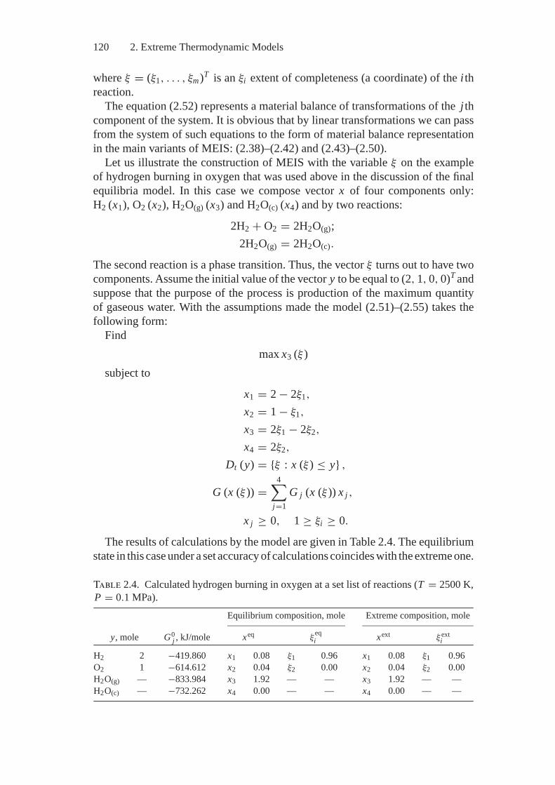
120 2. Extreme Thermodynamic Models
where ξ = (ξ1, . . . , ξm)T is an ξi extent of completeness (a coordinate) of the i threaction.
The equation (2.52) represents a material balance of transformations of the j thcomponent of the system. It is obvious that by linear transformations we can passfrom the system of such equations to the form of material balance representationin the main variants of MEIS: (2.38)–(2.42) and (2.43)–(2.50).
Let us illustrate the construction of MEIS with the variable ξ on the exampleof hydrogen burning in oxygen that was used above in the discussion of the finalequilibria model. In this case we compose vector x of four components only:H2 (x1), O2 (x2), H2O(g) (x3) and H2O(c) (x4) and by two reactions:
2H2 + O2 = 2H2O(g);2H2O(g) = 2H2O(c).
The second reaction is a phase transition. Thus, the vector ξ turns out to have twocomponents. Assume the initial value of the vector y to be equal to (2, 1, 0, 0)T andsuppose that the purpose of the process is production of the maximum quantityof gaseous water. With the assumptions made the model (2.51)–(2.55) takes thefollowing form:
Findmax x3 (ξ )
subject to
x1 = 2 − 2ξ1,
x2 = 1 − ξ1,
x3 = 2ξ1 − 2ξ2,
x4 = 2ξ2,
Dt (y) = {ξ : x (ξ ) ≤ y} ,
G (x (ξ )) =4∑
j=1G j (x (ξ )) x j ,
x j ≥ 0, 1 ≥ ξi ≥ 0.
The results of calculations by the model are given in Table 2.4. The equilibriumstate in this case under a set accuracy of calculations coincides with the extreme one.
Table 2.4. Calculated hydrogen burning in oxygen at a set list of reactions (T = 2500 K,P = 0.1 MPa).
Equilibrium composition, mole Extreme composition, mole
y, mole G0j , kJ/mole xeq ξ
eqi xext ξ ext
i
H2 2 −419.860 x1 0.08 ξ1 0.96 x1 0.08 ξ1 0.96O2 1 −614.612 x2 0.04 ξ2 0.00 x2 0.04 ξ2 0.00H2O(g) — −833.984 x3 1.92 — — x3 1.92 — —H2O(c) — −732.262 x4 0.00 — — x4 0.00 — —
2.3. Description of Different Types of Thermodynamic Systems 121
The hopes placed on the model (2.51)–(2.55) are associated with its applicationto the studies of mechanisms of chemical processes. The mechanism optimalin terms of maximizing the yield of a given set of substances is determined bymaking up the abundant list of reactions and automatically excluding unnecessarystages in the course of searching for ξ ext. It is possible to set the mechanisms thatcorrespond to different catalysts and compare the efficiency of the latter by theattained xext. Studies of such kind may certainly call for different modificationsof the model (2.51)–(2.55), for example, inclusion of additional constraints (onthe change in parameters of system, energy and mass exchange, etc.) or change inthe kind of constraints on the admissible values of x j and ξi (x j ≥ x j ≥ x j ; ξ i ≥ξi ≥ ξ j and so on). Doing this, as in the case of using the models (2.38)–(2.42)and (2.43)–(2.50), has nothing to do with the principal difficulties, since it doesnot change essentially the character of the mathematical programming problemssolved.
2.3. Description of Different Types ofThermodynamic Systems
Introductory NotesIn thermodynamics it is assumed that systems are divided into open, closed, andisolated; homogeneous and heterogeneous. The open systems can and the closedsystems cannot exchange matter with the environment. The isolated system ex-changes neither matter nor energy with other systems. The homogeneous sys-tems consist of a single and heterogeneous consist of several phases divided bysurfaces.
The properties of open and closed systems depend on the conditions of theirinteraction with the environment. The classical conditions of interaction and relatedequilibrium criteria are shown in Table I.1:
Further the systems can differ by the nature of forces in whose fields theyare located. Finally, a distinct feature of the system can be a character of spa-tial inhomogeneity, namely, changes along the coordinates of intensive parame-ters. The latter feature is often due to the specific nature of a field affecting thesystem.
Certainly, it is impossible to describe the whole variety of thermodynamic sys-tems, though the subject of thermodynamics encompasses the most general regu-larities of the macroworld. Here we will try to give only a preliminary set of modelsthat, on the one hand, will explain the technique of extreme descriptions account-ing for a specific nature of the systems to be modeled and, on the other hand, willreveal the advantages of the extreme thermodynamic approach on the whole.
First, let us consider the problems of modeling systems under different con-ditions of their interaction with the environment; next we will describe seperatephases of heterogeneous systems, and then give the models of spatially inhomo-geneous structures.
122 2. Extreme Thermodynamic Models
Description of the Conditions for the System Interactionwith the EnvironmentSince the above equilibrium conditions affect only the type of characteristic func-tion (that takes an extreme value), let us discuss only the impact these conditionshave on the model of xeq, which is a block of MEIS.
The most general model of the final equilibria is an isolated system model thatincludes a reaction mixture and thermal reservoir with which the reagents exchangeenergy. This model is written in terms of MP as follows:
Find
max
⎡⎢⎢⎢⎣
S (x, T, P) =∑
jS j
(T, Pj
)x j
+ T −1
(∑j
H yj y j −
∑j
Hj(T, Pj
)x j
)⎤⎥⎥⎥⎦ = S
(xeq) (2.56)
subject to
Ax = b, (2.57)∑j
H yj y j + H y
hr − H = 0, (2.58)
H =∑
jHj (T, P) x j + Hhr, (2.59)
f1 (T, P, V ) = 0, (2.60)Pj = f2 j (P, x) , (2.61)
Sj = f3 j (T, Pj ), Hj = f4 j (T, Pj ), (2.62)x j ≥ 0, (2.63)
where H yj is mole enthalpy of the j th initial reagent; H y
hr is enthalpy of the thermalreservoir in the initial state; H is total enthalpy of the system (a reaction mixtureand thermal reservoir).
The first term in the right-hand side of the expression in the square bracketsfor the objective function (2.56) is total entropy of the reagents, and the second isentropy transferred to the thermal reservoir. It is clear that the assumed equationof determining the latter is strictly satisfied only at a constant temperature ofthe reaction mixture. Otherwise, the integrals should be used in accordance withthe entropy determination. The equation (2.58) describes the condition of energyconservation. Certainly it can be simplified by excluding the term H y
hr, i.e., byassuming the initial enthalpy value of the thermal reservoir equal to zero. Theexpression (2.60) is the equation of the reaction mixture state.
From an extremality criterion for the isolated system (max S) we can pass tothe extremality criteria for its parts at fixed conditions of interaction among them,i.e., we can derive the criteria given in the beginning of the section. Thus, if T andP are maintained constant in the parts of the system, by substituting
Sj = (Hj − G j )T
2.3. Description of Different Types of Thermodynamic Systems 123
into (2.56) and by multiplying (2.56) by T , we can obtain a transformed criterion
max[
T S =∑
jHj x j −
∑j
G j x j +∑
jH y
j y j −∑
jHj x j
].
Taking into account that∑
jH y
j y j is a constant value we find that max S of
the system in this case corresponds to the max (−G) of its parts, and, hence,to min G. This explains the form of the objective function in the model (2.34)–(2.37).
Let us present the extreme models of xeq for two more important cases:
1) T = const, V = const:Find
min[
F (x) =∑
jFj (x) x j
]= F (xeq)
subject toAx = b, x j ≥ 0 ;
⎫⎪⎪⎪⎬⎪⎪⎪⎭
(2.64)
2) H = const, P = const:Find
max[
S (x, T ) =∑
jS j (x, T ) x j
]= S (xeq)
subject toAx = b,
∑j
Hj (x, T ) x j −∑
jH y
j y j = 0 ;
Hj = f1 j (T, x) , Sj = f2 j (T, x) , x j ≥ 0
⎫⎪⎪⎪⎪⎪⎪⎪⎬⎪⎪⎪⎪⎪⎪⎪⎭
(2.65)
Description of Multiphase SystemsThis book addresses the systems that may include:� an ideal gas phase;� real gases;� a plasma consisting of a neutral active species (radicals), ions, and electronic
gas;� pure condensed substances;� ideal solutions of electrically neutral substances and solutions of electrolytes;� ideal surface gas (ideal two-dimensional gas of the adsorbed substances on the
adsorbent surface);� substances in the colloidal (fine-disperse) state, the surfaces of whose particles
are subjected to surface tension forces.
The description of the ideal phases (gas, plasma, solution, surface gas) andpure condensed substances is based on the assumption that the thermodynamic
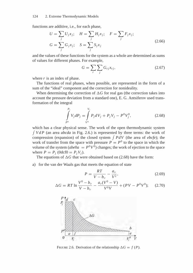
124 2. Extreme Thermodynamic Models
functions are additive, i.e., for each phase,
U =∑
jU j x j ; H =
∑j
Hj x j ; F =∑
jFj x j ;
G =∑
jG j x j ; S =
∑j
S j x j(2.66)
and the values of these functions for the system as a whole are determined as sumsof values for different phases. For example,
G =∑
r
∑j
Gr j xr j , (2.67)
where r is an index of phase.The functions of real phases, when possible, are represented in the form of a
sum of the “ideal” component and the correction for nonideality.When determining the correction of �G for real gas (the correction takes into
account the pressure deviation from a standard one), E. G. Antsiferov used trans-formation of the integral
Pj∫P0
Vj dPj =Vj∫
V 0
Pj dVj + Pj Vj − P0V 0j , (2.68)
which has a clear physical sense. The work of the open thermodynamic system∫V d P (an area abcda in Fig. 2.6.) is represented by three terms: the work of
compression (expansion) of the closed system∫
PdV (the area of ebcfe); thework of transfer from the space with pressure P = P0 to the space in which thevolume of the system (abe0a = P0V 0) changes; the work of ejection to the spacewhere P = Pj (0dcf0 = Pj Vj ).
The equations of �G that were obtained based on (2.68) have the form:
a) for the van der Waals gas that meets the equation of state
P = RTV − bυ
− aυ
V 2 , (2.69)
�G = RT ln V 0 − bυ
V − bυ
− aυ(V 0 − V )V 0V
+ (PV − P0V 0); (2.70)
Figure 2.6. Derivation of the relationship �G = f (P).
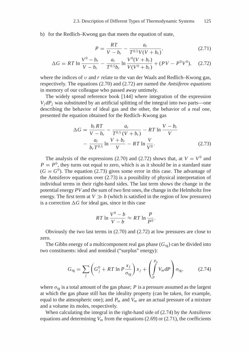
2.3. Description of Different Types of Thermodynamic Systems 125
b) for the Redlich–Kwong gas that meets the equation of state,
P = RTV − br
− ar
T 0.5V (V + br ) , (2.71)
�G = RT ln V 0 − br
V − br− ar
T 0.5brln V 0(V + br )
V (V 0 + br ) + (PV − P0V 0), (2.72)
where the indices of υ and r relate to the van der Waals and Redlich–Kwong gas,respectively. The equations (2.70) and (2.72) are named the Antsiferov equationsin memory of our colleague who passed away untimely.
The widely spread reference book [144] where integration of the expressionVj dPj was substituted by an artificial splitting of the integral into two parts—onedescribing the behavior of ideal gas and the other, the behavior of a real one,presented the equation obtained for the Redlich–Kwong gas
�G = br RTV − br
− ar
T 0.5 (V + br ) − RT ln V − br
V
− ar
br T 0.5 ln V + br
V− RT ln V
V 0 . (2.73)
The analysis of the expressions (2.70) and (2.72) shows that, at V = V 0 andP = P0, they turns out equal to zero, which is as it should be in a standard state(G = G0). The equation (2.73) gives some error in this case. The advantage ofthe Antsiferov equations over (2.73) is a possibility of physical interpretation ofindividual terms in their right-hand sides. The last term shows the change in thepotential energy PV and the sum of two first ones, the change in the Helmholtz freeenergy. The first term at V � b (which is satisfied in the region of low pressures)is a correction �G for ideal gas, since in this case
RT ln V 0 − bV − b
≈ RT ln PP0 .
Obviously the two last terms in (2.70) and (2.72) at low pressures are close tozero.
The Gibbs energy of a multicomponent real gas phase (Grg) can be divided intotwo constituents: ideal and nonideal (“surplus” energy):
Grg =∑
j
(G0
j + RT ln Px j
σrg
)x j +
⎛⎝ Pm∫
P
VmdP
⎞⎠ σrg, (2.74)
where σrg is a total amount of the gas phase; P is a pressure assumed as the largestat which the gas phase still has the ideality property (can be taken, for example,equal to the atmospheric one); and Pm and Vm are an actual pressure of a mixtureand a volume its moles, respectively.
When calculating the integral in the right-hand side of (2.74) by the Antsiferovequations and determining Vm from the equations (2.69) or (2.71), the coefficients
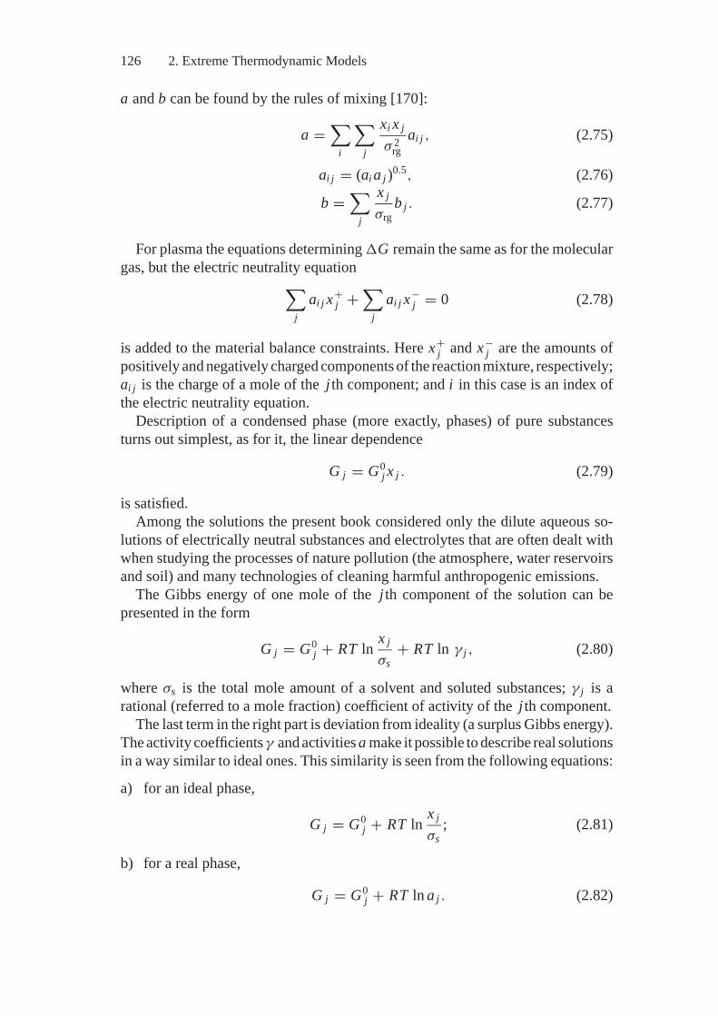
126 2. Extreme Thermodynamic Models
a and b can be found by the rules of mixing [170]:
a =∑
i
∑j
xi x j
σ 2rg
ai j , (2.75)
ai j = (aia j )0.5, (2.76)
b =∑
j
x j
σrgb j . (2.77)
For plasma the equations determining �G remain the same as for the moleculargas, but the electric neutrality equation∑
jai j x+
j +∑
jai j x−
j = 0 (2.78)
is added to the material balance constraints. Here x+j and x−
j are the amounts ofpositively and negatively charged components of the reaction mixture, respectively;ai j is the charge of a mole of the j th component; and i in this case is an index ofthe electric neutrality equation.
Description of a condensed phase (more exactly, phases) of pure substancesturns out simplest, as for it, the linear dependence
G j = G0j x j . (2.79)
is satisfied.Among the solutions the present book considered only the dilute aqueous so-
lutions of electrically neutral substances and electrolytes that are often dealt withwhen studying the processes of nature pollution (the atmosphere, water reservoirsand soil) and many technologies of cleaning harmful anthropogenic emissions.
The Gibbs energy of one mole of the j th component of the solution can bepresented in the form
G j = G0j + RT ln x j
σs+ RT ln γ j , (2.80)
where σs is the total mole amount of a solvent and soluted substances; γ j is arational (referred to a mole fraction) coefficient of activity of the j th component.
The last term in the right part is deviation from ideality (a surplus Gibbs energy).The activity coefficientsγ and activities a make it possible to describe real solutionsin a way similar to ideal ones. This similarity is seen from the following equations:
a) for an ideal phase,
G j = G0j + RT ln x j
σs; (2.81)
b) for a real phase,
G j = G0j + RT ln a j . (2.82)
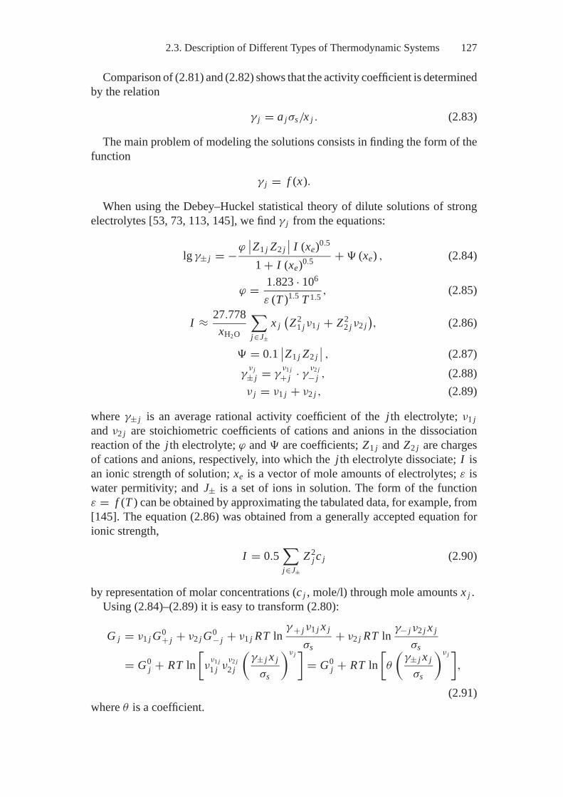
2.3. Description of Different Types of Thermodynamic Systems 127
Comparison of (2.81) and (2.82) shows that the activity coefficient is determinedby the relation
γ j = a jσs/x j . (2.83)
The main problem of modeling the solutions consists in finding the form of thefunction
γ j = f (x).
When using the Debey–Huckel statistical theory of dilute solutions of strongelectrolytes [53, 73, 113, 145], we find γ j from the equations:
lg γ± j = −ϕ∣∣Z1 j Z2 j
∣∣ I (xe)0.5
1 + I (xe)0.5 + � (xe) , (2.84)
ϕ = 1.823 · 106
ε (T )1.5 T 1.5 , (2.85)
I ≈ 27.778xH2O
∑j∈J±
x j(Z2
1 jν1 j + Z22 jν2 j
), (2.86)
� = 0.1∣∣Z1 j Z2 j
∣∣ , (2.87)γ
ν j± j = γ
ν1 j+ j · γ
ν2 j− j , (2.88)
ν j = ν1 j + ν2 j , (2.89)
where γ± j is an average rational activity coefficient of the j th electrolyte; ν1 jand ν2 j are stoichiometric coefficients of cations and anions in the dissociationreaction of the j th electrolyte; ϕ and � are coefficients; Z1 j and Z2 j are chargesof cations and anions, respectively, into which the j th electrolyte dissociate; I isan ionic strength of solution; xe is a vector of mole amounts of electrolytes; ε iswater permitivity; and J± is a set of ions in solution. The form of the functionε = f (T ) can be obtained by approximating the tabulated data, for example, from[145]. The equation (2.86) was obtained from a generally accepted equation forionic strength,
I = 0.5∑j∈J±
Z2j c j (2.90)
by representation of molar concentrations (c j , mole/l) through mole amounts x j .Using (2.84)–(2.89) it is easy to transform (2.80):
G j = ν1 j G0+ j + ν2 j G0
− j + ν1 j RT lnγ + jν1 j x j
σs+ ν2 j RT ln γ− jν2 j x j
σs
= G0j + RT ln
[ν
ν1 j1 j ν
ν2 j2 j
(γ± j x j
σs
)ν j]= G0
j + RT ln[θ
(γ± j x j
σs
)ν j],
(2.91)where θ is a coefficient.
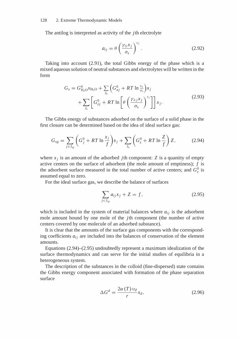
128 2. Extreme Thermodynamic Models
The antilog is interpreted as activity of the j th electrolyte
ai j = θ
(γ±x j
σs
)ν j
. (2.92)
Taking into account (2.91), the total Gibbs energy of the phase which is amixed aqueous solution of neutral substances and electrolytes will be written in theform
Gs = G0H2OxH2O + ∑
Jn
(G0
nj + RT ln x jσs
)x j
+∑
Je
[G0
ej + RT ln[θ
(γ± j x j
σs
)ν j]]x j .
(2.93)
The Gibbs energy of substances adsorbed on the surface of a solid phase in thefirst closure can be determined based on the idea of ideal surface gas:
Gsg =∑j∈Jsg
(G0
j + RT ln x j
f
)x j +
∑Jn
(G0
z + RT ln Zf
)Z , (2.94)
where x j is an amount of the adsorbed j th component: Z is a quantity of emptyactive centers on the surface of adsorbent (the mole amount of emptiness); f isthe adsorbent surface measured in the total number of active centers; and G0
z isassumed equal to zero.
For the ideal surface gas, we describe the balance of surfaces∑j∈Jsg
ai j x j + Z = f , (2.95)
which is included in the system of material balances where ai j is the adsorbentmole amount bound by one mole of the j th component (the number of activecenters covered by one molecule of an adsorbed substance).
It is clear that the amounts of the surface gas components with the correspond-ing coefficients ai j are included into the balances of conservation of the elementamounts.
Equations (2.94)–(2.95) undoubtedly represent a maximum idealization of thesurface thermodynamics and can serve for the initial studies of equilibria in aheterogeneous system.
The description of the substances in the colloid (fine-dispersed) state containsthe Gibbs energy component associated with formation of the phase separationsurface
�Gd = 2α (T ) υd
rxd , (2.96)
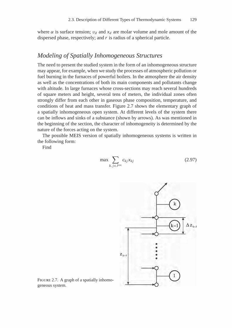
2.3. Description of Different Types of Thermodynamic Systems 129
where α is surface tension; υd and xd are molar volume and mole amount of thedispersed phase, respectively; and r is radius of a spherical particle.
Modeling of Spatially Inhomogeneous StructuresThe need to present the studied system in the form of an inhomogeneous structuremay appear, for example, when we study the processes of atmospheric pollution orfuel burning in the furnaces of powerful boilers. In the atmosphere the air densityas well as the concentrations of both its main components and pollutants changewith altitude. In large furnaces whose cross-sections may reach several hundredsof square meters and height, several tens of meters, the individual zones oftenstrongly differ from each other in gaseous phase composition, temperature, andconditions of heat and mass transfer. Figure 2.7 shows the elementary graph ofa spatially inhomogeneous open system. At different levels of the system therecan be inflows and sinks of a substance (shown by arrows). As was mentioned inthe beginning of the section, the character of inhomogeneity is determined by thenature of the forces acting on the system.
The possible MEIS version of spatially inhomogeneous systems is written inthe following form:
Find
max∑
k, j∈J ext
ck j xk j (2.97)
Figure 2.7. A graph of a spatially inhomo-geneous system.
130 2. Extreme Thermodynamic Models
subject to
Ax = b, (2.98)Ainσ = Q, (2.99)
�z1 P1σkTk − �zk Pkσ1T1 = 0, k = 1, . . . , K (2.100)Dt (y) = {x : x ≤ y} , (2.101)
(x) =∑k j
k j (x) xk j , j = 1, . . . , n, (2.102)
k j(g) = G0k j (Tk) + RT ln
(Pk
xk
σk
)+ M j gzk, (2.103)
k j(c) = G0k j(c) (Tk) + 2α j Vj
rk j, (2.104)
xk j ≥ 0, (2.105)
where x and xk j are a vector of substance amounts and its kjth component, respec-tively; Ain is a matrix of incidences (connections) of independent nodes and arcsof the graph mapping the system structure; σ = (σ1, . . . , σk)T is a vector of totalsubstance amounts in the regions (on the graph arcs); Q is a vector of externalinflows and sinks; zk and �zk are a vertical coordinate in the middle of the kthzone and a thickness of the gas layer modeled by it, respectively; and k j aregeneralized Gibbs energy of the system and a potential of the kjth component,respectively; g is free fall acceleration; and index “1” relates to the zone with theminimum zk .
The model (2.97)–(2.105) includes two material balances: the first of them (2.98)represents the condition for mass conservation of elements in chemical reactionsand phase transitions; the second balance (2.100) is the expression of the firstKirchhoff law (mass conservation at matter transfer along the branches of thesystem graph). Equation (2.100) is based on the assumption that the gas phasein each zone is ideal and describes the bond between the substance quantities inindividual zones.
The generalized Gibbs energy in the model (2.97)–(2.105) represents the sumof chemical, gravity, and surface (associated with formation of phase interfaces)components. The form of the function can be found by the technique of trans-forming the thermodynamic equilibrium equation. The technique was illustratedby a number of examples in Section 1.3. In the given case for the gaseous phasesuch an equation will be written in the form
V dp + Mgdz +∑
jμ j dx j − SdT = 0, (2.106)
where the terms on the left-hand side represent the works of the forces of pressure,gravity, chemical interactions, and elementary thermal impact, respectively. Since
V dp +∑
jμ j dx j − SdT = dG
2.3. Description of Different Types of Thermodynamic Systems 131
(see equation 1.21), the equation (2.106) is transformed to the form
dG + mgdz = 0. (2.107)
Thus the form of the function to be minimized becomes clear
=∑
j
(G j + M j gdz
)x j . (2.108)
From (2.106) we can derive the equation of distribution of pressure and densitythroughout the height of the gas column:
P∫P0
V dp = RTP∫
P0
dpP
= −Mgz∫
0
dz −∑
jμ j dx j + S
T∫T 0
dT ,
P = P0 exp
⎡⎢⎢⎣−
Mgz +∑
jμ j dx j − S(T − T 0)
RT
⎤⎥⎥⎦ , (2.109)
where index “0” refers to the zero level of z. The equation (2.109) represents theBoltzmann distribution that takes into account gravitational, chemical, and thermaleffects in the gas phase.
The form of the correction for the Gibbs energy of the condensed phase associ-ated with the action of the surface tension force (the second term in the right-handside of (2.104)) has already been discussed above. Equation (2.104), unlike ex-pression (2.103) for of the gas phase, does not include the components M j gzkbecause the action of gravitantional forces on condensed particles is balanced byresistance forces whose field is not a potential. Therefore, it is impossible (or verydifficult) to associate the solution to the equilibrium problem of these two types offorces with the solution to the extreme problem. At the same time their equilibriumdoes not affect the remaining equilibria that take place in the heterogeneous systemand can be excluded from consideration.
Let us make an additional comment to explain the model (2.97)–(2.105). Inho-mogeneity of the modeled system is represented in a “discreet” form in it. It isdistributed among the final number of zones, each supposed to be homogeneous.Location of these zones in space can be presented in the form of a graph and thelaws of conservation in the processes of substance and energy exchanges betweenthe zones are presented in a network form. This explains the interpretation of(2.99) as a form of the first Kirchhoff law for the flows of the matter moving alonga hydraulic circuit. It is clear that, according to the thermodynamic approach, thedescription of such a motion is reduced to the description of states of rest.
The use of the model (2.97)–(2.105) for the analysis of real objects can beillustrated by the calculation of substance distribution in the vertical air column ofthe isothermic atmosphere 5 km high. We divide this column into five zones, perconvention, each one kilometer high, and suppose that on the system graph thereis one node with the substance’s inflow (0) and one with its sink (k). The assumed
132 2. Extreme Thermodynamic Models
scheme can be understood if we imagine that up to some time instant there is noair above the earth’s surface, and then it is gradually supplied to node 0 and fromthe node k with the sink, as a result of this motion, the air is distributed throughoutthe height of the vertical column.
The chosen initial set of reagents (y) and the results of calculations of states xeq
and xextH2O(g) are presented in Table 2.5. The values in the columns xext are obtained
by a number of calculations. Each calculation is the supposed search for the max-imum concentration of one of the four components: NO2, CO, HNO3, and O3. Forthe remaining components of the system the extreme concentrations are not calcu-lated. Similar calculations are discussed in detail in Section 5.1, which is speciallydedicated to the thermodynamic analysis of atmospheric pollution processes. Inthis section we only note that at highly idealized assumption (the atmosphere isisothermal; there is no condensed phase) the calculations performed confirm atleast to some extent the correctness of the model (2.97)–(2.105) suggested by theauthors. Thus, altitudinal distribution of each component x j turned out to satisfythe Boltzmann distribution
xk j = x1 j exp(
− M j gzk
RT
), (2.110)
and the impact of chemical reactions on the exponent index almost did not manifestitself. The results of these calculations correspond to the experimental data in [25].
We should also comment on the numerical values of xk j presented in Table 2.5.Certainly, there is no physical sense in determining the concentrations of atmo-spheric components of less than 10−20–10−25. At such low densities of the matter,thermodynamics laws cease to obtain. The aim of including such extremely accu-rate results into Table 2.5 is only to demonstrate the reliability of the computationalgorithm that allows solution of the problem with a great scatter in values ofvariables. The computational aspect of the thermodynamic analysis is consideredin Chapter 4.
2.4. Mathematical Features of theExtreme Thermodynamic Models
Introductory RemarksIt is necessary to understand the mathematical features of the extreme modelsdiscussed both for development of effective methods and computational algorithmsand for correct physical interpretation of the problems studied with these models.Indeed, there is a strong tie between the mathematical and physical nature ofscientific problems. Below, as applied to the presented mathematical programmingmodels, consider the specific features of the objective functions F (x, y), systemsof constraints and extreme solutions: xeq, xext, and (xext, yext). The main problemof the analysis is, undoubtedly, the estimation of whether it is possible to reducethese extreme problems to the CP problems. The CP are subject to formalized
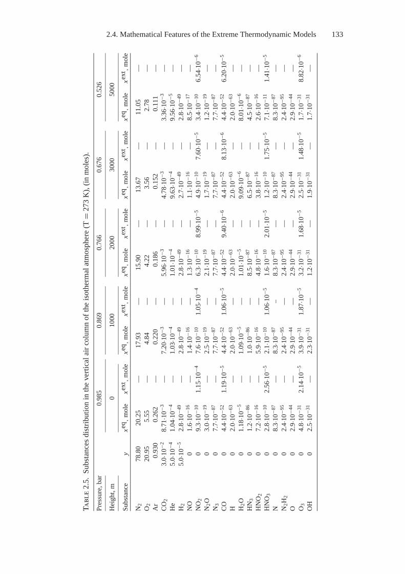
2.4. Mathematical Features of the Extreme Thermodynamic Models 133
Tabl
e2.
5.Su
bsta
nces
distr
ibut
ion
inth
ever
tical
airc
olum
nof
thei
soth
erm
alat
mos
pher
e(T
=27
3K
),(in
mol
es).
Pres
sure
,bar
0.98
50.
869
0.76
60.
676
0.52
6
Hei
ght,
m0
1000
2000
3000
5000
Subs
tanc
ey
xeq ,
mol
exe
xt,
mol
exe
q ,m
ole
xext
,m
ole
xeq ,
mol
exe
xt,
mol
exe
q ,m
ole
xext
,m
ole
xeq ,
mol
exe
xt,
mol
e
N2
78.8
020
.25
—17
.93
—15
.90
—13
.67
—11
.05
—O
220
.95
5.55
—4.
84—
4.22
—3.
56—
2.78
—A
r0.
930
0.26
2—
0.22
0—
0.18
6—
0.15
2—
0.11
1—
CO2
3.0·1
0−2
8.71
·10−3
—7.
20·10
−3—
5.96
·10−3
—4.
78·10
−3—
3.36
·10−3
—H
e5.
0·10−
41.
04·10
−4—
1.03
·10−4
—1.
01·10
−4—
9.63
·10−4
—9.
56·10
−5—
H2
5.0·1
0−5
2.8·1
0−49
—2.
8·10−
49—
2.8·1
0−49
—2.
7·10−
49—
2.8·1
0−49
—N
O0
1.6·1
0−16
—1.
4·10−
16—
1.3·1
0−16
—1.
1·10−
16—
8.5·1
0−17
—N
O2
09.
3·10−
101.
15·10
−47.
6·10−
101.
05·10
−46.
3·10−
108.
99·10
−54.
9·10−
107.
60·10
−53.
4·10−
106.
54·10
−6N
2O0
3.0·1
0−19
—2.
5·10−
19—
2.1·1
0−19
—1.
7·10−
19—
1.2·1
0−19
—N
30
7.7·1
0−87
—7.
7·10−
87—
7.7·1
0−87
—7.
7·10−
87—
7.7·1
0−87
—CO
04.
4·10−
521.
19·10
−54.
4·10−
521.
06·10
−54.
4·10−
529.
40·10
−64.
4·10−
528.
13·10
−64.
4·10−
526.
20·10
−5H
02.
0·10−
63—
2.0·1
0−63
—2.
0·10−
63—
2.0·1
0−63
—2.
0·10−
63—
H2O
01.
18·10
−5—
1.09
·10−5
—1.
01·10
−5—
9.09
·10−6
—8.
01·10
−6—
HN
30
1.2·1
0−86
—1.
0·10−
86—
8.5·1
0−87
—6.
5·10−
87—
4.5·1
0−87
—H
NO
20
7.2·1
0−16
—5.
9·10−
16—
4.8·1
0−16
—3.
8·10−
16—
2.6·1
0−16
—H
NO
30
2.8·1
0−10
2.56
·10−5
2.1·1
0−10
1.06
·10−5
1.6·1
0−10
2.01
·10−5
1.2·1
0−10
1.75
·10−5
7.1·1
0−11
1.41
·10−5
N0
8.3·1
0−87
—8.
3·10−
87–
8.3·1
0−87
—8.
3·10−
87—
8.3·1
0−87
—N
2H2
02.
4·10−
95—
2.4·1
0−95
—2.
4·10−
95—
2.4·1
0−95
—2.
4·10−
95—
O0
2.9·1
0−44
—2.
9·10−
44—
2.9·1
0−44
—2.
9·10−
44—
2.9·1
0−44
—O
30
4.8·1
0−31
2.14
·10−5
3.9·1
0−31
1.87
·10−5
3.2·1
0−31
1.68
·10−5
2.5·1
0−31
1.48
·10−5
1.7·1
0−31
8.82
·10−6
OH
02.
5·10−
31—
2.3·1
0−31
—1.
2·10−
31—
1.9·1
0−31
—1.
7·10−
31—
134 2. Extreme Thermodynamic Models
interpretations and their numerical solutions are much easier than the multicriteriaproblems of concave programming (see Section 2.1).
To prove that the applied model belongs to the CP models it is necessary to revealthe concave or linear character of the maximized function (convexity or linearityof the minimized one) and convexity of Dt (y). The latter is to a large extentdetermined by the character of the thermodynamic functions: U , H , F , G, and S.Like V , these functions are known to be extensive thermodynamic parameters andare homogeneous functions of the first power, that is, they satisfy the relationship
f (kx1, . . . , kxn) = k f (x1, . . . , xn) . (2.111)
The intensive thermodynamic parameters T , P , μ, mole energy, and mole en-tropy are homogeneous functions of the zero power for which
f (kx1, . . . , kxn) = k0 f (x1, . . . , xn) = f (x1, . . . , xn) . (2.112)
For homogeneous functions the Euler equationn∑
j=1
∂ f (x1, . . . , xn)∂x j
x j = λ f (x1, . . . , xn) , (2.113)
is true where λ is a power of the homogeneous function. For ideal systems, U , H ,F , G, S have the additivity property, which was explained in previous sections.However, for our analysis, it is most important to confirm the convexity propertyin these functions (for S, concavity), which is caused by the uniqueness of thepoint xeq (see below). A strict convexity analysis of the thermodynamic functionsin ideal systems is presented in a number of works (see [58, 167, 177]). As appliedto real systems, the authors here consider these points in [81, 83]. As the convexityproblem is very important, the whole section will be dedicated to it below, buthere the MEIS features will be analyzed assuming convexity of thermodynamicfunctions.
Specific Features of the Block x eq
In the block (2.34)–(2.37) of the general MEIS, the Gibbs energy is the objectivefunction. At its convexity the region of the thermodynamic attainability Dt (y) thatrepresents part of the material balance polyhedron also becomes convex. Indeed,assume that there are two points x ′ ∈ Dt (y) and x ′′ ∈ Dt (y), i.e., such points thateach of them can be reached from the initial state y by continuous trajectories thatentirely belong to Dt (y) and, along the what trajectories the Gibbs energy does notincrease. However, then meeting the thermodynamic constraints, it is possible, iwwe start the motion from y, to attain any point z of the section [x ′, x ′′] either alongthe path y − x ′ − z or along the path y − x ′′ − z, as the convex function G (x)on either of the sections [x ′, z] and [x ′′, z] does not necessarily increase. Hence,along with the points x ′ and x ′′ that belong to Dt (y), any point x of the sectionconnecting them belongs to the same set. Therefore, the set Dt (y) is convex. Thus,the search for xeq belongs to CP problems.
2.4. Mathematical Features of the Extreme Thermodynamic Models 135
Here, if the studied system is ideal or reduceable to the ideal—for example, byintroducing the notion of activity, that is,
G j = G0j + f
(ln x j
), (2.114)
the point xeq is an interior point of Dt (y) and all the components of vector x arecontained in it, even if in negligibly small quantities.
Suppose the opposite, namely, that in the equilibrium state the amount ofthe j th component equals zero. Consider the behavior of the function G (x) onthe section [xeq, xρ], where xρ is the point in which x j > 0. Obviously, on thebalance polyhedron (2.35) denoted below by D (y), such a point can be found. Byvirtue of the fact that the derivative of G (x) with respect to x j at x j = 0 goes to−∞ in a rather small vicinity of xeq on the section [xeq, xρ], there will be a pointwhose j th coordinate will be strictly positive (since xρ
j > 0) and the value of G (x)will be less than the value at the point G (xeq), a situation that is impossible. It isclear that with the presence of condensed substances in the mixture, the point xeq
by the corresponding coordinates can be located on the boundary line of Dt (y).Certainly the presented property of the point xeq is satisfied only within applica-
bility of the equilibrium thermodynamics itself. When the concentration of somecomponent of xeq
j is so insignificant that statistical rules cannot be applied to it,the strict inequality
xeqj > 0 for all j = 1, . . . , n,
can be employed to analyze the behavior of mathematical models of type (2.34)–(2.37), but it cannot be extensively interpreted as applied to real objects.
There is another specific feature of the systems that obey equation (2.114). Thisfeature is very important for the development of computational algorithms andanalysis of solutions. It consists of this: If the line of the constant level D (y)passing via some vertex of G (x) does not contain any other point of the materialbalance polyhedron, then there is a region of thermodynamic unattainability nearthis vertex and it is impossible to get to this region from any other point of thepolyhedron. The vertex itself in this case is the point of local maximum of the Gibbsenergy. The presence of condensed phases in the system may lead to the absence ofunattainability regions at some vertices (the minimum of G j (x) of liquid and solidsubstances is located at the points x j = 0). In the case where the line G (x) = constpassing through a vertex crosses the interior region of D (y), several vertices atonce can belong to the thermodynamic unattainability region.
In concluding the discussion of the specific features of the model xeq we notethat the possibility of its reduction to the CP problem is not affected by the presenceof condensed phases in the modeled system. Here the mathematical characteristicsof the model are essentially improved owing to the above (see Section 2.2) de-scription of individual phases of one and the same substance by different variables(components of vector x). This fact is illustrated by Fig. 2.8.
Suppose that some substance A is formed in the course of chemical relaxation.In the initial period of formation, A is contained only in the gas phase, and itsGibbs energy with the increasing amount xA changes along the curve 1, which
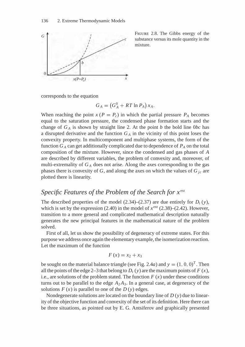
136 2. Extreme Thermodynamic Models
G
b
x(P=Pc)
c
x0
Figure 2.8. The Gibbs energy of thesubstance versus its mole quantity in themixture.
corresponds to the equation
G A = (G0
A + RT ln PA)
xA.
When reaching the point x (P = Pc) in which the partial pressure PA becomesequal to the saturation pressure, the condensed phase formation starts and thechange of G A is shown by straight line 2. At the point b the bold line 0bc hasa disrupted derivative and the function G A in the vicinity of this point loses theconvexity property. In multicomponent and multiphase systems, the form of thefunction G A can get additionally complicated due to dependence of PA on the totalcomposition of the mixture. However, since the condensed and gas phases of Aare described by different variables, the problem of convexity and, moreover, ofmulti-extremality of G A does not arise. Along the axes corresponding to the gasphases there is convexity of G, and along the axes on which the values of G jc areplotted there is linearity.
Specific Features of the Problem of the Search for x ext
The described properties of the model (2.34)–(2.37) are due entirely for Dt (y),which is set by the expression (2.40) in the model of xext (2.38)–(2.42). However,transition to a more general and complicated mathematical description naturallygenerates the new principal features in the mathematical nature of the problemsolved.
First of all, let us show the possibility of degeneracy of extreme states. For thispurpose we address once again the elementary example, the isomerization reaction.Let the maximum of the function
F (x) = x2 + x3
be sought on the material balance triangle (see Fig. 2.4a) and y = (1, 0, 0)T . Thenall the points of the edge 2–3 that belong to Dt (y) are the maximum points of F (x),i.e., are solutions of the problem stated. The function F (x) under these conditionsturns out to be parallel to the edge A2 A3. In a general case, at degeneracy of thesolutions F (x) is parallel to one of the D (y) edges.
Nondegenerate solutions are located on the boundary line of D (y) due to linear-ity of the objective function and convexity of the set of its definition. Here there canbe three situations, as pointed out by E. G. Antsiferov and graphically presented
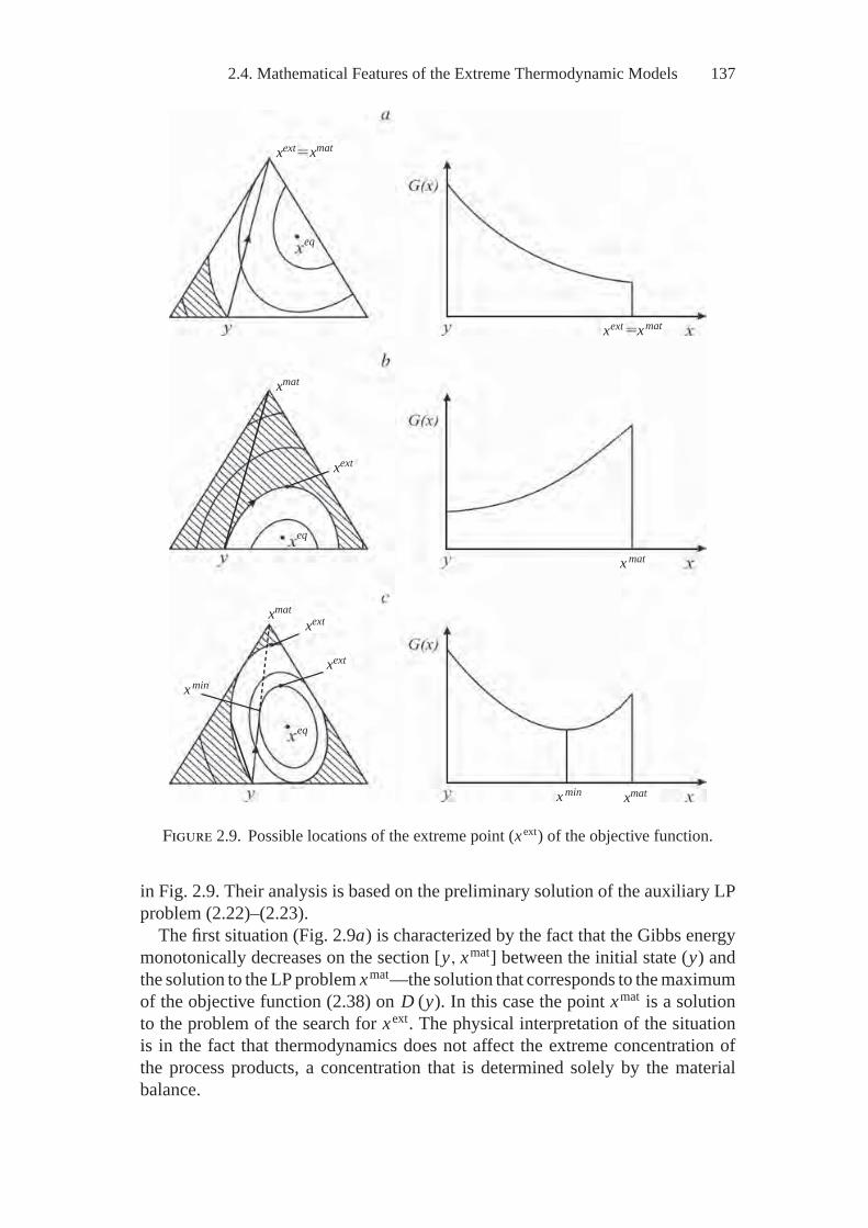
2.4. Mathematical Features of the Extreme Thermodynamic Models 137
eq
eq
eq
xmat
xmat
xmat
xmat
x min
x min
xext
xmatxext
xext
xext
xext
x mat
Figure 2.9. Possible locations of the extreme point (x ext) of the objective function.
in Fig. 2.9. Their analysis is based on the preliminary solution of the auxiliary LPproblem (2.22)–(2.23).
The first situation (Fig. 2.9a) is characterized by the fact that the Gibbs energymonotonically decreases on the section [y, xmat] between the initial state (y) andthe solution to the LP problem xmat—the solution that corresponds to the maximumof the objective function (2.38) on D (y). In this case the point xmat is a solutionto the problem of the search for xext. The physical interpretation of the situationis in the fact that thermodynamics does not affect the extreme concentration ofthe process products, a concentration that is determined solely by the materialbalance.
138 2. Extreme Thermodynamic Models
From the mathematical viewpoint the problem is transformed into the canonicLP problem coinciding with the mentioned auxiliary one:
Find
max(
F (x) =∑
jc j x j
)= F(xext)
subject to ∑j
ai j x j = bi , x j ≥ 0, i = 1, . . . , m, j = 1, . . . , n ;
⎫⎪⎪⎪⎪⎪⎬⎪⎪⎪⎪⎪⎭
(2.115)
It follows that the extremum point is located in one of the D (y) vertices andthe number of nonzero components xext = xmat does not exceed m—the numberof material balance equations. As is clear from the analysis of the problem of thesearch for xeq, the first situation may appear either in the absence of unattainabilityregions in the vicinity of some vertices or in the case when these regions arenegligibly small.
In the second situation (Fig. 2.9b) in the direction from y to xmat the Gibbsenergy increases continuously and, hence, motion along the section [y, xmat] turnsout to be impossible. The search for maximum concentrations is reduced to thefollowing CP problem:
Find
max(
F (x) =∑
jc j x j
)= F(xext)
subject to ∑j
ai j x j = bi , x j ≥ 0, i = 1, . . . , m, j = 1, . . . , n,
G (x) ≤ G (y) .
⎫⎪⎪⎪⎪⎪⎪⎪⎬⎪⎪⎪⎪⎪⎪⎪⎭
(2.116)
The point xext is located on the initial surface of the Gibbs energy G = G (y).The value of the objective function in this case meets the condition
F(y) ≤ F(xext) ≤ F(xmat). (2.117)
The third situation (Fig. 2.9c) consists in the fact that on the section [y, xmat]there is a minimum of G (point xmin). The point xext turns out to be located on theboundary line of Dt (y). The problem of determining its location is considered inChapter 3. The CP problem solved takes the following form:
Find
max(
F (x) =∑
jc j x j
)= F(xext)
subject to ∑j
ai j x j = bi , x j ≥ 0, i = 1, . . . , m, j = 1, . . . , n,
G (x) ≤ G(xext).
⎫⎪⎪⎪⎪⎪⎪⎪⎬⎪⎪⎪⎪⎪⎪⎪⎭
(2.118)
2.4. Mathematical Features of the Extreme Thermodynamic Models 139
Solution of the problem (2.118) as well as that of (2.116), meets the conditionof (2.117). Further, this third situation will be called “a thermodynamic pothole.”
The mathematical nature of the problem of searching for xext gets essentiallymore complicated in the cases where the system of constraints includes nonlinearenergy balances (at fixing H and P , or U and V ) or nonlinear entropy balances(at fixing S and P , or S and V ).
Thus, at constant H and P , on the way from y to xmat we should observe thenonlinear enthalpy balance and, hence, the section [y, xmat] becomes curvilinear.Under these circumstances it is sensible to replace the point xmat by xm.h in whichthe objective function extreme is attained and simultaneously the material andenthalpy balances are met.
However, the difficulties that arise can be overcome by the transition from thespace (x, T ) to the space x , at which, as will be shown in Section 2.5, the concavityof entropy and convexity of Dt (y) are maintained. Such a transition makes thestudies of the systems with given U and V , S and P , or S and V mathematicallysimilar to the study of systems with fixed T and P , or T and V .
Perhaps the last specific feature of the model xext worth mentioning is the im-plicitly set constraints on the change in thermodynamic functions (the expression(2.40)), which, to an essential extent, complicates the construction of computa-tional algorithms for solution of the problem of type (2.38)–(2.42).
Analysis of the Problem of the Search for the Point (x ext , yext)The general problem (2.43)–(2.50) of the search for the point (xext, yext) differsfrom the blocks of xeq and xext, first of all, by nonlinearity and fractional char-acter of the objective function. To represent objective function form on the linearpolyhedron (2.45), (2.46), (2.50) at a varying initial composition of reagents, wesuppose that the mole number of the j th component whose extremum is soughtfor is determined by the expression
x j = yρ − ερ , (2.119)where yρ is an initial reagent involved in the reaction of x j formation and theonly initial reagent whose economical use is of interest to us; ερ is an unreactedpart of yρ .
With the taken assumptions, which simplify the problem significantly, the ob-jective function and the Lagrange function of the system (2.43)–(2.46) takes theform
F (x, y) = x j/yρ = (yρ − ερ
)/yρ (2.120)
and
L = yρ − ερ
yρ
+ λ1
(1 −
l∑j=1
M j y j
)+
m+1∑i=2
λi
(bi −
∑j
ai j x j
)
+2m+1∑
i=m+2λi
(bi −
∑j
ai j y j
), (2.121)
140 2. Extreme Thermodynamic Models
and two first derivatives of the Lagrange function turn out to be equal to
∂L∂yρ
= ερ
y2ρ
− λ1 Mρ −2m+1∑
i=m+2λi aiρ, (2.122)
∂2L∂y2
ρ
= −2ερ
y3ρ
≤ 0. (2.123)
From this follows the concavity of the function (2.43) by y for the consideredcase. Obviously, a similar proof can be given for the somewhat less strict con-straints than those assumed above, for example, for the situation where we areinterested in the economical use of several reagents, and in which the relation-ship between x j and yρ gets more complicated as compared to equality (2.119).In all the previous studies on the model (2.43)–(2.50) there were no deviationsfrom concavity of F (x, y). Hence, at least in many cases, the problem (2.43)–(2.50) at maximization of F (x, y) is reduced to a CP problem. However, in thefuture the character of the objective function of MEIS should be analyzed morestrictly.
The problem of finding the value of y, optimal in terms of minimizationof F(x) relates to concave mathematical programming, and it is of a multi-extreme character. Practically, the solution of this problem is very importantin creating environmentally friendly technologies (the search for the most en-vironmentally benign composition of reagents) and, therefore, is worth furtherscrutiny.
Another important distinction of the model (2.43)–(2.50) from the models(2.34)–(2.37), and (2.38)–(2.42) is that it does not contain explicit relationshipsbetween the values of vectors x and y and, therefore, it is not possible to find theanalytical expressions for the derivatives
∂F (x, y)∂y
.
A feature that imposes constraints on the choice of computational algorithms.In conclusion of this section we would like to make a comment on MEIS con-
cerning the variables ξ . Transition from the space x to the space ξ is due toreplacement of the material balance polyhedron
Ax = b, x ≥ 0,
by the polyhedron
νξ = xe − y, ξ ≥ 0, (2.124)
with the edges of unit length along the coordinate axes (see condition (2.55)). In(2.124) ν is a vector of stoichiometric coefficients: xe is a value of the vector xprovided that all the reactions are completed (ξ = 1 for all i = 1, . . . , m). Sucha linear transformation of balance equations seems not to affect noticeably themathematical nature of the problem stated.
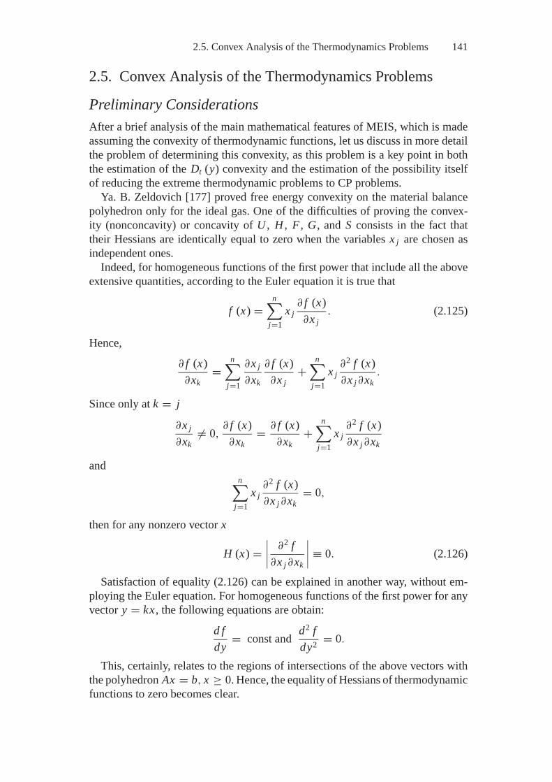
2.5. Convex Analysis of the Thermodynamics Problems 141
2.5. Convex Analysis of the Thermodynamics Problems
Preliminary ConsiderationsAfter a brief analysis of the main mathematical features of MEIS, which is madeassuming the convexity of thermodynamic functions, let us discuss in more detailthe problem of determining this convexity, as this problem is a key point in boththe estimation of the Dt (y) convexity and the estimation of the possibility itselfof reducing the extreme thermodynamic problems to CP problems.
Ya. B. Zeldovich [177] proved free energy convexity on the material balancepolyhedron only for the ideal gas. One of the difficulties of proving the convex-ity (nonconcavity) or concavity of U , H , F , G, and S consists in the fact thattheir Hessians are identically equal to zero when the variables x j are chosen asindependent ones.
Indeed, for homogeneous functions of the first power that include all the aboveextensive quantities, according to the Euler equation it is true that
f (x) =n∑
j=1x j
∂ f (x)∂x j
. (2.125)
Hence,∂ f (x)∂xk
=n∑
j=1
∂x j
∂xk
∂ f (x)∂x j
+n∑
j=1x j
∂2 f (x)∂x j∂xk
.
Since only at k = j
∂x j
∂xk�= 0,
∂ f (x)∂xk
= ∂ f (x)∂xk
+n∑
j=1x j
∂2 f (x)∂x j∂xk
andn∑
j=1x j
∂2 f (x)∂x j∂xk
= 0,
then for any nonzero vector x
H (x) =∣∣∣∣ ∂2 f∂x j∂xk
∣∣∣∣ ≡ 0. (2.126)
Satisfaction of equality (2.126) can be explained in another way, without em-ploying the Euler equation. For homogeneous functions of the first power for anyvector y = kx , the following equations are obtain:
d fdy
= const and d2 fdy2 = 0.
This, certainly, relates to the regions of intersections of the above vectors withthe polyhedron Ax = b, x ≥ 0. Hence, the equality of Hessians of thermodynamicfunctions to zero becomes clear.
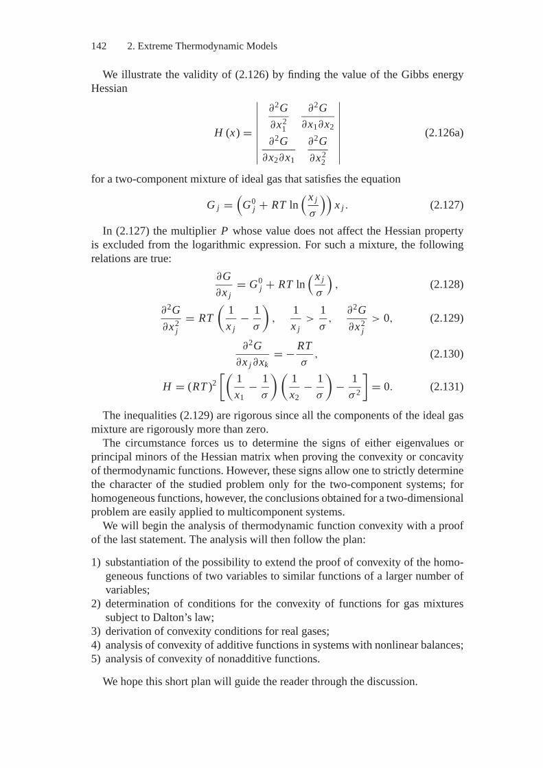
142 2. Extreme Thermodynamic Models
We illustrate the validity of (2.126) by finding the value of the Gibbs energyHessian
H (x) =
∣∣∣∣∣∣∣∣∣
∂2G∂x2
1
∂2G∂x1∂x2
∂2G∂x2∂x1
∂2G∂x2
2
∣∣∣∣∣∣∣∣∣(2.126a)
for a two-component mixture of ideal gas that satisfies the equation
G j =(
G0j + RT ln
( x j
σ
))x j . (2.127)
In (2.127) the multiplier P whose value does not affect the Hessian propertyis excluded from the logarithmic expression. For such a mixture, the followingrelations are true:
∂G∂x j
= G0j + RT ln
( x j
σ
), (2.128)
∂2G∂x2
j= RT
( 1x j
− 1σ
),
1x j
>1σ
,∂2G∂x2
j> 0, (2.129)
∂2G∂x j∂xk
= − RTσ
, (2.130)
H = (RT )2[( 1
x1− 1
σ
)( 1x2
− 1σ
)− 1
σ 2
]= 0. (2.131)
The inequalities (2.129) are rigorous since all the components of the ideal gasmixture are rigorously more than zero.
The circumstance forces us to determine the signs of either eigenvalues orprincipal minors of the Hessian matrix when proving the convexity or concavityof thermodynamic functions. However, these signs allow one to strictly determinethe character of the studied problem only for the two-component systems; forhomogeneous functions, however, the conclusions obtained for a two-dimensionalproblem are easily applied to multicomponent systems.
We will begin the analysis of thermodynamic function convexity with a proofof the last statement. The analysis will then follow the plan:
1) substantiation of the possibility to extend the proof of convexity of the homo-geneous functions of two variables to similar functions of a larger number ofvariables;
2) determination of conditions for the convexity of functions for gas mixturessubject to Dalton’s law;
3) derivation of convexity conditions for real gases;4) analysis of convexity of additive functions in systems with nonlinear balances;5) analysis of convexity of nonadditive functions.
We hope this short plan will guide the reader through the discussion.
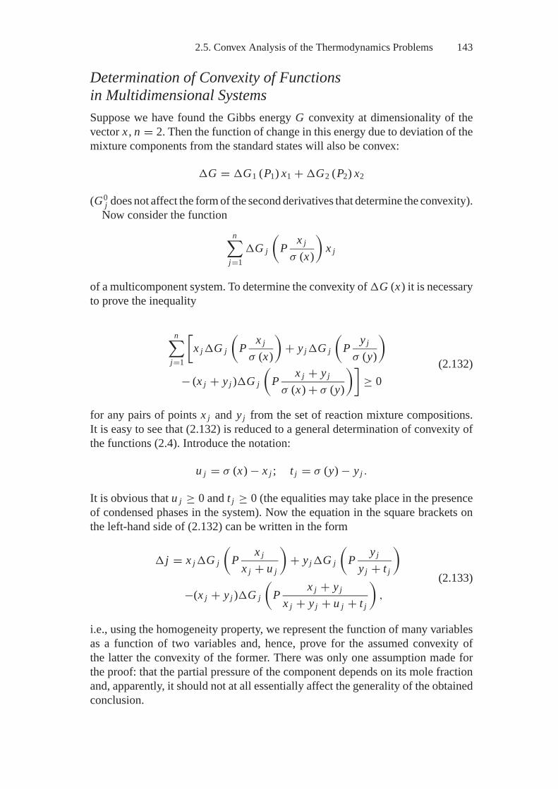
2.5. Convex Analysis of the Thermodynamics Problems 143
Determination of Convexity of Functionsin Multidimensional SystemsSuppose we have found the Gibbs energy G convexity at dimensionality of thevector x , n = 2. Then the function of change in this energy due to deviation of themixture components from the standard states will also be convex:
�G = �G1 (P1) x1 + �G2 (P2) x2
(G0j does not affect the form of the second derivatives that determine the convexity).
Now consider the functionn∑
j=1�G j
(P
x j
σ (x)
)x j
of a multicomponent system. To determine the convexity of �G (x) it is necessaryto prove the inequality
n∑j=1
[x j�G j
(P
x j
σ (x)
)+ y j�G j
(P
yj
σ (y)
)
− (x j + y j )�G j
(P
x j + y j
σ (x) + σ (y)
)]≥ 0
(2.132)
for any pairs of points x j and y j from the set of reaction mixture compositions.It is easy to see that (2.132) is reduced to a general determination of convexity ofthe functions (2.4). Introduce the notation:
u j = σ (x) − x j ; t j = σ (y) − y j .
It is obvious that u j ≥ 0 and t j ≥ 0 (the equalities may take place in the presenceof condensed phases in the system). Now the equation in the square brackets onthe left-hand side of (2.132) can be written in the form
� j = x j�G j
(P
x j
x j + u j
)+ y j�G j
(P
yj
y j + t j
)
−(x j + y j )�G j
(P
x j + y j
x j + y j + u j + t j
),
(2.133)
i.e., using the homogeneity property, we represent the function of many variablesas a function of two variables and, hence, prove for the assumed convexity ofthe latter the convexity of the former. There was only one assumption made forthe proof: that the partial pressure of the component depends on its mole fractionand, apparently, it should not at all essentially affect the generality of the obtainedconclusion.
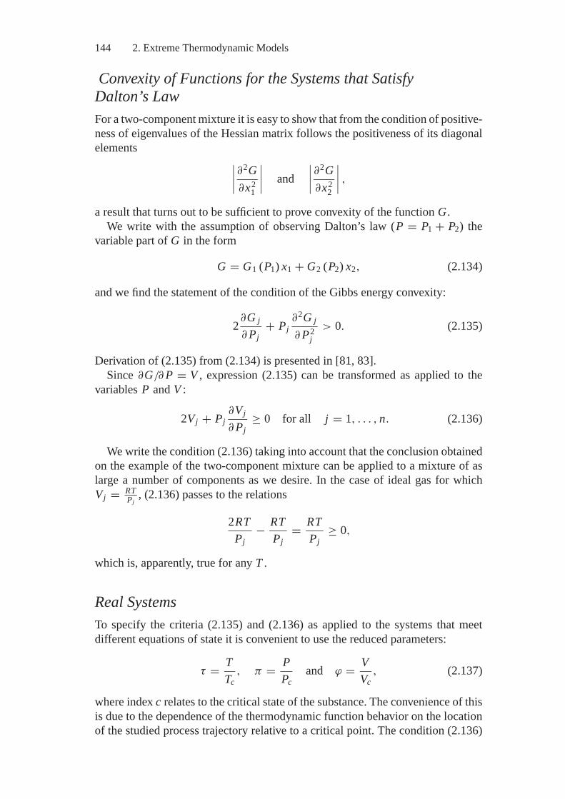
144 2. Extreme Thermodynamic Models
Convexity of Functions for the Systems that SatisfyDalton’s LawFor a two-component mixture it is easy to show that from the condition of positive-ness of eigenvalues of the Hessian matrix follows the positiveness of its diagonalelements ∣∣∣∣∂2G
∂x21
∣∣∣∣ and∣∣∣∣∂2G∂x2
2
∣∣∣∣ ,a result that turns out to be sufficient to prove convexity of the function G.
We write with the assumption of observing Dalton’s law (P = P1 + P2) thevariable part of G in the form
G = G1 (P1) x1 + G2 (P2) x2, (2.134)
and we find the statement of the condition of the Gibbs energy convexity:
2∂G j
∂ Pj+ Pj
∂2G j
∂ P2j
> 0. (2.135)
Derivation of (2.135) from (2.134) is presented in [81, 83].Since ∂G/∂ P = V , expression (2.135) can be transformed as applied to the
variables P and V :
2Vj + Pj∂Vj
∂ Pj≥ 0 for all j = 1, . . . , n. (2.136)
We write the condition (2.136) taking into account that the conclusion obtainedon the example of the two-component mixture can be applied to a mixture of aslarge a number of components as we desire. In the case of ideal gas for whichVj = RT
Pj, (2.136) passes to the relations
2RTPj
− RTPj
= RTPj
≥ 0,
which is, apparently, true for any T .
Real SystemsTo specify the criteria (2.135) and (2.136) as applied to the systems that meetdifferent equations of state it is convenient to use the reduced parameters:
τ = TTc
, π = PPc
and ϕ = VVc
, (2.137)
where index c relates to the critical state of the substance. The convenience of thisis due to the dependence of the thermodynamic function behavior on the locationof the studied process trajectory relative to a critical point. The condition (2.136)
2.5. Convex Analysis of the Thermodynamics Problems 145
in the given coordinates takes the form
2ϕ j (π j ) + π j∂ϕ j
∂π j≥ 0. (2.138)
The algorithm for determination of the convexity conditions of G at a set equa-tion of state is reduced to the following procedures:� Using a number of transformations the criterion (2.138) is replaced by the
inequality�(ϕ j , τ j ) ≥ 0,
where � is monotonically increasing function τ .� The values ϕ j and τ j are found for the case where the equality
�(ϕ j , τ j ) = 0corresponds to the minimum of �, and for this purpose the system of equations
∂�
∂τ= 0, �(ϕ j , τ j ) = 0 (2.139)
is solved.At values τ equal to or larger than the obtained solution of (2.139), G of the
system turns out to be a strictly convex function due to monotonicity of �. Thecondition (2.139) is sufficient but not necessary. Indeed, the convexity region mayappear to be somewhat larger than what follows from the condition.
For the gas mixture obeying the equation of van der Waals that, in the givencoordinates, has the form
π = 8τ/
(3ϕ − 1) − 3ϕ−2, (2.140)the function � is determined by the expression1
�(ϕ j , τ j ) = 83ϕ2
j (3ϕ j + 1) − 3(3ϕ j − 1)2, (2.141)
1 We present the derivation of the equation that determines the value � j(ϕ j , τ j
), for the
van der Waals gas. First, find the set of values τ for which ϕ j(π j
)satisfies the condition
(2.138). It is obvious thatdπ j
dϕ j· dϕ j
dπ j= 1 and ϕ′
j (π j ) = 1π ′ j (ϕ j )
.
Substituting the expression for ϕ′j (π j ) into (2.138) we obtain
2ϕ j + π j/π′j (ϕ j ) ≥ 0.
Since the derivative of the reduced pressure with respect to the reduced volume for the vander Waals gas
π ′j (ϕ j ) = −24τ j (3ϕ j − 1)−2 + 6ϕ−3
j (2.140a)at τ > 1 is always negative, the condition of convexity (2.136) can be rewritten in the form
2ϕ j (π j )π ′jϕ(ϕ, τ ) + π j (ϕ, τ ) ≤ 0.
Substituting the values π j and π ′j from (2.140) and (2.140a) into this expression and making
elementary transformations, we find that �(ϕ j , τ j ) is determined by the equation (2.141).
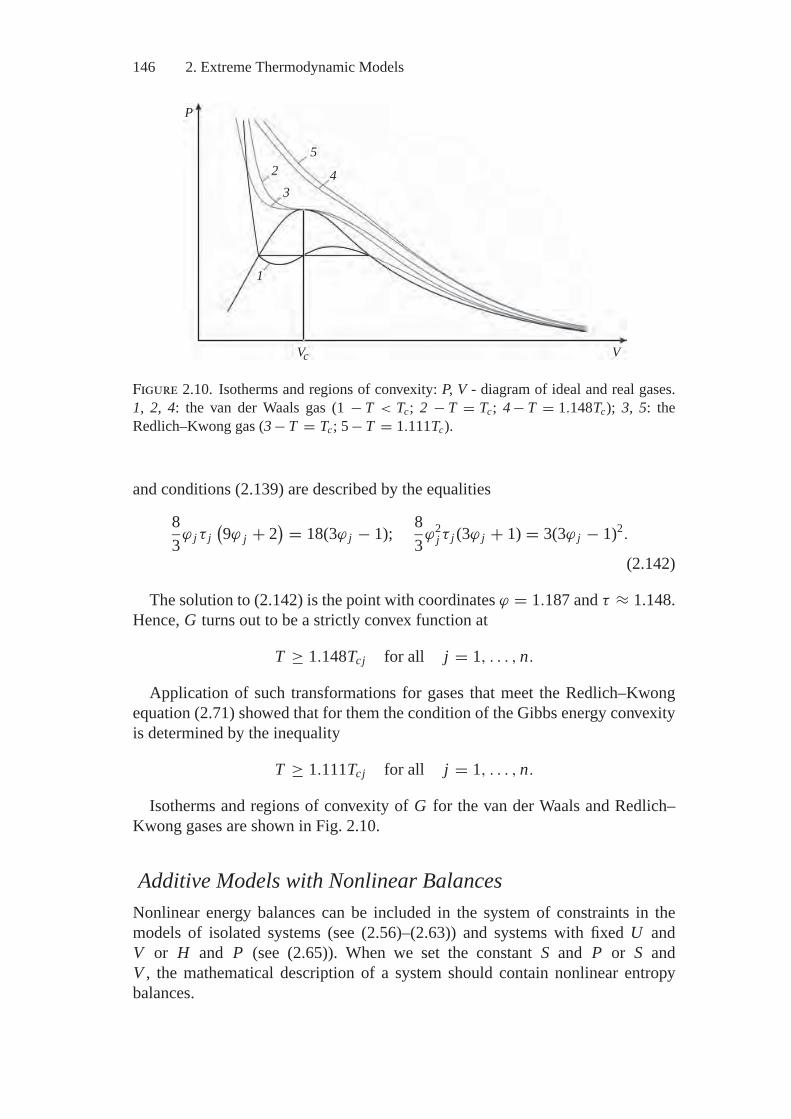
146 2. Extreme Thermodynamic Models
P
23
5
4
VVc
1
Figure 2.10. Isotherms and regions of convexity: P, V - diagram of ideal and real gases.1, 2, 4: the van der Waals gas (1 − T < Tc; 2 − T = Tc; 4 − T = 1.148Tc); 3, 5: theRedlich–Kwong gas (3 − T = Tc; 5 − T = 1.111Tc).
and conditions (2.139) are described by the equalities
83ϕ jτ j
(9ϕ j + 2
) = 18(3ϕ j − 1); 83ϕ2
j τ j (3ϕ j + 1) = 3(3ϕ j − 1)2.
(2.142)
The solution to (2.142) is the point with coordinates ϕ = 1.187 and τ ≈ 1.148.Hence, G turns out to be a strictly convex function at
T ≥ 1.148Tcj for all j = 1, . . . , n.
Application of such transformations for gases that meet the Redlich–Kwongequation (2.71) showed that for them the condition of the Gibbs energy convexityis determined by the inequality
T ≥ 1.111Tcj for all j = 1, . . . , n.
Isotherms and regions of convexity of G for the van der Waals and Redlich–Kwong gases are shown in Fig. 2.10.
Additive Models with Nonlinear BalancesNonlinear energy balances can be included in the system of constraints in themodels of isolated systems (see (2.56)–(2.63)) and systems with fixed U andV or H and P (see (2.65)). When we set the constant S and P or S andV , the mathematical description of a system should contain nonlinear entropybalances.
2.5. Convex Analysis of the Thermodynamics Problems 147
Along the axes of x j the objective functions of the models with nonlinear con-straints retain all the above specific features. For example, using the transforma-tions similar to those made when analyzing the convexity of G it is possible toshow that the condition of entropy convexity on the polyhedron D (y) at constantH , P and T has the form:
2 ∂Sj
∂ Pj+ Pj
∂2Sj
∂ P2j
≤ 0 (2.143)
or
− 1T
(2V
(Pj
) + Pj∂Vj
∂ Pj
)≤ 0. (2.144)
To study the extreme properties of the model (2.65) in coordinates x , T weconstruct the Lagrange function, supposing that the reagents represent a mixtureof ideal gases and P = 1 (the latter supposition, obviously, does not affect theresults of analysis):
L =n∑
j=1
(S0
j (T ) − R ln( x j
σ
))x j +
m∑i=1
λi
(bi −
n∑j=1
ai j x j
)
+ λm+1
[H y −
n∑j=1
Hj(x j , T
)x j
]. (2.145)
To get the equations of derivatives of L with respect to x and T let us makeanother simplifying assumption: that the relationship between the isobaric heatcapacity and the temperature is expressed by the equation
cp = α + βT . (2.146)
Such a binomial approximation of the function cp (T ) in this case is quite suffi-cient, since at α ≥ 0 and β ≥ 0 it correctly shows the monotonically nondecreasingcharacter of this function and, hence, the convexity of H (T ).
With satisfaction of (2.146) and assumption that Sj (0) = 0 and cpj (0) = 0,
S0j (T ) =
T∫0
(α j + β j T
)T
dT = α j ln T + β j T, (2.147)
Hj (T ) =T∫
0
(α j + β j T )dT + �Hj (0) = α j T + 0.5β j T 2 + �Hj (0) ,
(2.148)
where �Hj (0) is the enthalpy of the j th component formation at 0 K.Taking into account (2.147) and (2.148), we find the first and second derivatives
148 2. Extreme Thermodynamic Models
of L with respect to x j and T :
∂L∂x j
= S0j (T ) − R ln
(x j/σ
) −m∑
i=1λi ai j − λm+1 Hj (T ) , (2.149)
∂2L∂x2
j= −R
( 1x j
− 1σ
), (2.150)
∂L∂T
= 1T
∑j
(α j + β j T
)x j − λm+1
∑j
(α j + β j T
)x j , (2.151)
∂2L∂T 2 = − 1
T 2
∑j
α j x j − λm+1∑
jβ j x j .
Since at the derivative (2.151) equal to zero (which is true at equilibrium)
λm+1 = 1/T, (2.152)
then∂2L∂T 2 = − 1
T 2
∑j
α j x j − 1T
∑j
β j x j . (2.153)
From the equality of (2.150) we can conclude that
−R( 1
x j− 1
σ
)< 0 (2.154)
is the condition of the entropy concavity along the axes x j . This inequality is strictsince for ideal mixtures x j > 0 for all j = 1, . . . , n. The mathematical relationbetween (2.154) and the condition (2.144) can easily be found.
From (2.153) it follows that concavity of L with respect to T is determined bythe equation
− 1T 2
∑j
α j x j − 1T
∑j
β j x j ≤ 0,
which is equivalent to the condition
− 1T 2
∑j
cpj x j ≤ 0, (2.155)
Which, in turn, is always satisfied due to positiveness of cP .Thus, the conditions of interaction with the environment and related nonlinear
balances practically do not affect the convexity of the thermodynamic functions. Iteven appears possible, maintaining the convexity of the functions, to simplify theproblem by passing from the space x , T to the space x and get rid of the nonlinearconstraint
n∑j=1
Hj (T ) x j − H y = 0, (2.156)
an approach that is convenient in terms of calculations.
2.5. Convex Analysis of the Thermodynamics Problems 149
Indeed, due to monotonicity of the functionn∑
j=1Hj x j = H (T )
temperature can be presented as a single-valued function x :
T = T (x) .
To find the extreme properties of the transformed model for the systems withH = const and P = const, note that we have already proved the concavity∑
j�Sj
(Pj
) �= f (T )
and so we determine the character of the function
S (x, T (x)) =n∑
j=1S0
j (T (x)) x j . (2.157)
For this purpose we find the first and second derivatives of S (x, T (x)) with respectto some coordinate xk .
The first derivative is∂S (x, T (x))
∂xk=
∑j
∂S0j (T )∂T
∂T (x)∂xk
x j + S0k (T (x)) . (2.158)
To obtain the equation for ∂T (x)∂xk
we use the derivative
∂
∂xk
(n∑
j=1Hj (T (x)) x j − H y
)=
n∑j=1
∂ Hj (T )∂T
∂T∂xk
x j + Hk (T ) .
Taking into account that this derivative equals zero, we find∂T (x)∂xk
= − Hk (T )n∑
j=1x j cpj
since ∂ Hj (T )∂T = cpj .
Bearing in mind that∂S0
j (T )∂T
= cpj
T,
we have that∂S (x, T (x))
∂xk= − Hk (T )
T+ S0
k (T (x)) = −G0k (T )T
. (2.159)
The second derivative
∂2S (x, T (X ))∂x2
k= − ∂
∂xk
(G0
k (T )T
)= − H 2
k (T )T 2
(n∑
j=1x j cpj
)−1
. (2.160)
150 2. Extreme Thermodynamic Models
It is obvious that this is always less than zero and at transition from the space x, Tto the space x , the problem discussed still belongs to CP problems.
Nonadditive Heterogeneous ModelsNonadditive systems comprise practically all the real systems, since there is alwaysinteraction to some or another extent between particles of different types and,hence, the expressions for entropy and energy should contain the terms that reflectthis interaction.
First of all, we point out that the nonadditive models have a very importantproperty in terms of mathematical analysis: It consists in the fact that the molethermodynamic functions of the j th component are not derivatives of the corre-sponding functions of the system with respect to x j , i.e.,
G j �= ∂G∂x j
, Fj �= ∂F∂x j
, Hj �= ∂ H∂x j
, U j �= ∂U∂x j
, Sj �= ∂S∂x j
. (2.161)
We write the Gibbs energy of the nonadditive system in the form similar to thatassumed for description of the ideal mixtures,
G =n∑
j=1
[G0
j + RT ln(γ j (x) x j
σ
)]x j , (2.162)
where γ is an activity coefficient.The simplest transformations show that
∂G∂xk
= G0k + RT ln γk (x) xk
σ+ RT
n∑j=1
x j
γ j (x)∂γ j (x)
∂xk, (2.163)
and the molar Gibbs energy
Gk = G0k + RT ln
[γk (x) xk
σ
]does not equal ∂G/∂xk and, hence, is not a potential. Thus, the conditions of phaseequilibrium of nonadditive systems do not consist in the equality of molar Gibbsenergies of one and the same substance in different phases, but in the equalityof derivatives ∂G/∂xk . This is seen from the expression for the derivative of theLagrange function:
L =n∑
j=1G j x j +
m∑i=1
λi
(bi −
n∑j=1
ai j x j
), (2.164)
∂L∂x j
= ∂G∂x j
+m∑
i=1λi ai j = 0 (2.165)
(the derivative equality to zero corresponds to the equilibrium state).Since, for the components of vector x that meet different phases of some sub-
stance, the coefficients of ai j are equal and the derivatives of ∂G/∂xk are equal,too.
2.5. Convex Analysis of the Thermodynamics Problems 151
Note that according to the Euler equation, for homogeneous functions,n∑
k=1xk
n∑j=1
x j
∂γ j (x)∂γ j (x)
∂xk≡ 0, (2.166)
i.e., the total value of the latter terms on the right-hand sides of the equations oftype (2.163) equals zero and the Gibbs energy of a nonadditive mole mixture as awhole retains the property of the potential, which is natural.
The conditions for convexity of the Gibbs energy function of nonadditive modelswere analyzed on the example of the van der Waals gas for which we obtainedcomparatively simple dependences that can be quantitatively analyzed.
When using the equations (2.70) and (2.75)–(2.77) the convexity criterion takesthe form
∂2G∂x2
j= RT
( 1x j
− 1σ
)+ RT
(b j − b
)2
σ
( 1(V − b)2 − 1
(V 0 − b)2
)
− 2(V 0 − b)V 0V
a0.5j
σ(a0.5
j − a) ≥ 0, j = 1, . . . , n.
(2.167)
In (2.167), the first term is the second derivative of the Gibbs function of idealgas, the second one takes into account the impact of repulsion forces, and the thirdterm takes into account the attraction forces between particles. The analysis ofequation (2.167) shows that the convexity condition can be violated in the caseswhen the third term being negative sign exceeds in absolute value the sum of thefirst two terms in the absolute value. A preliminary consideration shows that thiscan take place only at very high pressures and is unlikely under real conditions.
Thus, the discussions of different types of models in this section make it clearthat though the convexity of thermodynamic functions can be strictly determinedonly under a number of simplifying assumptions on the physics of the studiedprocesses, the assumption on the convexity turns out acceptable for solution of awide range of practical problems. This, certainly, does not deny the need to developthe convex analysis of thermodynamic models.
3Thermodynamic Modeling on Graphs
Formulas are written figures.Figures are drawn formulas.
D. Hilbert
3.1. Problem Statement and History
The question on the effectiveness of geometrical methods for development andinterpretation of extreme thermodynamic models is evidently subject to essentialsubjectivism and partiality. So, whereas Newton in his Principles started to solveeach of more than 200 considered problems with graphical explanations, and onlythen passed to formulas, Lagrange in Mechanique Analytique did not present anydrawings, demonstrating thus the possibility of constructing the “building” ofmechanics without graphical representation.
Though in thermodynamics, geometrical methods have been applied startingwith Gibbs’s classical works, in the works known to the authors on computermodeling of thermodynamic systems, such methods have not been practicallyused. Our reference to graphical construction is based on the assumption thatgraphs should provide an insight into mathematical peculiarities of the problemssolved, on the one hand, and contribute to expansion of the sphere for applicationsof extreme models, on the other.
Yet Kirchhoff had shown the possibility of reducing problems dealing with thestudy on multidimensional systems to problems on graphs. In [111] he tested therevealed theoretical relationships for current and potential distribution in the flatround plate by comparison with the experimental results on the electric circuit,i.e., on the object with the scheme in a graph form. Thus, he established thecorrespondence between electric fields in the continuous two-dimensional spaceand on the one-dimensional continuum, i.e., the “graph.” Kirchhoff deduced hisknown laws of current distribution for graphs and showed in [112] how to derivean independent system of equations by using these laws, choosing the calculated
152
3.1. Problem Statement and History 153
loops corresponding to chords, that is, edges that remain after separation of thespanning tree from the closed graph.
In later works on the theory of electric circuits [108–110] Kirchhoff factu-ally constructed a complete system of models to study these circuits. In [108] heshowed the possibility of a transition from solving a closed system of equations(of Kirchhoff’s laws) to the extreme problem – the search for the minimum heatgeneration in a passive circuit (one without sources of electromotive forces). Toput it differently, he suggested an extreme model of current distribution. In [109,110] the motion equation (the Ohm law) is derived in terms of the equilibrium offorces acting on “electric liquids,” and the considered equilibrium in this case canbe interpreted as the thermodynamic one.
Kirchhoff’s works make clear the possibility of equivalent mutual transfor-mations of models that are based on different physical principles (conservation,equilibrium, extremality); Kirchhoff’s analysis alse substantiates the transitionfrom such models, including extreme thermodynamic multidimensional systems,to graphical models.
Maxwell suggested the method of potentials [129] for calculation of electricalcircuits as graphs, which is equivalent to the method of loop currents based onKirchhoff’s circuit laws of conservation. At about the same time Gibbs introducedin the thermodynamics the method of potentials for multidimensional continua[53].
Geometrical methods were developed by A. N. Gorban in Equilibrium Encir-cling for thermodynamic analysis of chemical system kinetics. These methodsmade it possible for one to pass from searching the extremum of the Lyapunovthermodynamic function on the material balance polyhedron to searching for it onthe graph called a thermodynamic tree. This tree vividly and simply represents anaggregate of paths along which the Lyapunov function changes monotonically andthe sets of compositions attainable from the initial state of a system (the thermo-dynamic attainability region). It is constructed by the relations of thermodynamicequivalence of x1 and x2: That is, x1 ∼ x2 if there exists a continuous curve runningfrom the composition x1 to the composition x2 along which the thermodynamicLyapunov function is constant. Identification of thermodynamically equivalentcompositions with respect to each other enables transformation of the domain ofdefinition of the studied function to one-dimensional space, namely the tree, whichfacilitates substantially the analysis of processes in chemical systems.
Studies similar to those performed by A.N. Gorban, but belonging to pure math-ematics were conducted by A.S. Kronrod [116] and V.I. Arnold [10]. Their workswere aimed at solving the thirteenth Hilbert problem, i.e., representation of thecontinuous function of many variables as a superposition of continuous functionsof a lesser number of variables [69]. A.S. Kronrod suggested a method to trans-form a multidimensional domain of definition of functions into a one-dimensionalcontinuum, the tree of functions (which can be handled as the mathematical gen-eralization of the notion of the thermodynamic tree); V.I. Arnold applied such atree to obtain exact and approximate representations of some specific functions.
154 3. Thermodynamic Modeling on Graphs
In our opinion the idea of a tree is interesting from the general principles ofmathematical programming (MP)—the principles for solving extreme problems.Actually each MP method is characterized by the rule that determines at each step ofthe computational process a direction of motion and a path length over the functionsurface whose extremum is sought for. If we use the tree with set initial state andconvexity of considered function, our choice of trajectory becomes unambiguous.
Note also the paper by A.I. Volpert [168], in which bichromatic graphs areapplied to the qualitative analysis of solutions to differential equations of def-inite form for the problems of chemical kinetics. The work [28] presents arather wide view of the application of topology and theory of graphs to quantumchemistry.
B.M. Kaganovich employed extreme thermodynamic models to study hydrauliccircuits [77–79], i.e., objects whose structure is naturally represented as graphs. Inso doing, he proceeded from the concepts of the hydraulic circuit theory (HCT),which was founded by V.Ya. Khasilev and A.P. Merenkov [104–107, 132, 130].
Creation of extreme thermodynamic models of flow distribution in circuits andphysical interpretation of HCT on their basis provided a deeper insight into thistheory, facilitated correct comparison of its methods, and enhanced potential of itsapplications. Thus, the low sensitivity of extreme methods to change in the spaceof variables made a wide variation of problem statements possible, e.g., inclusionof diverse constraints on parameter regulation in the models of post-emergencyregimes of pipeline networks. The ideas of thermodynamic modeling of hydraulicsystems may turn out to be useful in studying electric networks as well.
As a result of the thermodynamic analysis of HCT the problem of modelingheterogeneous hydraulic circuits (i.e., circuits with multiphase chemically reactingflows in the branches, or graph arcs was formulated in [91]. Studies of this problemsubstantially extended an area of HCT applications.
B.M. Kaganovich also made attempts to employ jointly thermodynamics andthe hydraulic circuit theory to analyze multidimensional continua. The works [81,83, 85] interpret model of extreme intermediate states (MEIS) with the variable ξ inthe graphical form and represent some other extreme models of chemical systemswith the specified mechanism of reactions in the form of hydraulic systems. In [91]MEIS of spatially inhomogeneous structures, which is somewhat different than themodel of (2.97)–(2.105), is interpreted as a hydraulic circuit to study atmosphericpollution processes.
Descriptions of continua in the form of circuits certainly make sense, if for noother reason than the joint analysis of several possible mathematical models of oneand the same object contributes to deeper understanding of it’s the object’s physicalproperties. On the whole, graphical models are useful in substantiating applicabilityof thermodynamics concepts to different types of physicochemical systems. If wemanage to represent the studied function as a function of no more than two variablesfor each graph branch, then because of the holonomy of the corresponding Pfaffianforms it becomes possible to prove its possible representation as a differentiablepotential function, which determines applicability of thermodynamics techniques.
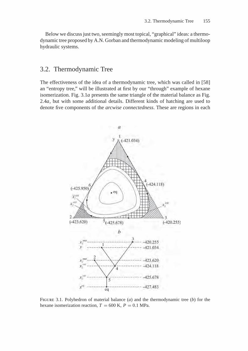
3.2. Thermodynamic Tree 155
Below we discuss just two, seemingly most topical, “graphical” ideas: a thermo-dynamic tree proposed by A.N. Gorban and thermodynamic modeling of multiloophydraulic systems.
3.2. Thermodynamic Tree
The effectiveness of the idea of a thermodynamic tree, which was called in [58]an “entropy tree,” will be illustrated at first by our “through” example of hexaneisomerization. Fig. 3.1a presents the same triangle of the material balance as Fig.2.4a, but with some additional details. Different kinds of hatching are used todenote five components of the arcwise connectedness. These are regions in each
Figure 3.1. Polyhedron of material balance (a) and the thermodynamic tree (b) for thehexane isomerization reaction, T = 600 K, P = 0.1 MPa.
156 3. Thermodynamic Modeling on Graphs
of which any two points can be connected by a thermodynamically admissiblepath.
Fig. 3.1b shows the thermodynamic tree whose branches have a one-to-onecorrespondence with the regions hatched in Fig. 3.1a. Every point of the tree rep-resents an intercept of a line G = const belonging to the corresponding componentof connectedness. The points on this intercept satisfy the linear balance:∑
jG j x j = G = const. (3.1)
The constructed tree that replaces the polyhedron D (y) allows the study on thebehavior of the Gibbs energy (a thermodynamic Lyapunov function in this case)and the objective function (2.38). Suppose that the initial state y is representedby the vertex 1 (y = (1, 0, 0)T ) and the process objective is to obtain a maximumpossible quantity of the isomer x3 (the objective function (2.38) takes the formF (x) = x3). The desired maximum point on D (y) is obviously vertex 3. We canmove to it from y along tree branch 1–4, monotonically decreasing the functionG (x). However, after point 4 is reached, further movement to 3 becomes impossiblebecause the Gibbs energy monotonically increases on branch 3–4 from 4 towards3. Point 4 determines a level of G (the isopotential surface of G = −424.118kJ/mole), at which the extreme composition xext
3 (the linear function maximum isachieved at the convex set boundary) should lie.
With the choice of vertex 2 as an initial state y and the new maximization of x3,the solution will be on the surface G5 = −425.678 kJ/mole. When we maximizex2 the same Gibbs energy level is attained from the initial states 1 and 3.
Note that when we solve all the mentioned problems:
y = (1, 0, 0)T , max x3,
y = (0, 1, 0)T , max x3,
y = (1, 0, 0)T , max x2,
y = (0, 0, 1)T , max x2,
there is a situation of the “thermodynamic pothole,” for which we cannot indicatethe exact Gibbs energy levels G
(xext) (see Section 2.4). Application of the tree
overcomes the difficulty that arises. Fig. 3.1a illustrates a potential benefit thanksto improvement of the obtained problem solution by the thermodynamic tree. Ifwe moved from vertex 1 to vertex 2 (tending to max x2), reached the point min Gon the intercept 1–2 (point 6) and then continued to move along the curve G = G6,we would be able to reach the point xext
2 , which contains the component x2in asomewhat lesser amount than at the point of exact solution xext
2 (the errors ofdifferent algorithms are discussed in Chapter 4).
The tree can be applied to the analysis of situations, when the stated problem’ssolution proves to be degenerate. For hexane isomerization such a situation occursat maximization of the total amount of any two components and at equality ofeach coefficient c j in (2.38) to unity (see Section 2.4). If we find, for example,max (x2 + x3) and y = (1, 0, 0)T , all the points of edge 2–3 (Fig. 3.1a) belonging
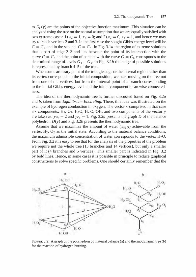
3.2. Thermodynamic Tree 157
to Dt (y) are the points of the objective function maximum. This situation can beanalyzed using the tree on the natural assumption that we are equally satisfied withtwo extreme cases: 1) x2 = 1, x3 = 0; and 2) x2 = 0, x3 = 1, and hence we maytry to reach vertices 2 and 3. In the first case the sought Gibbs energy level will beG = G5 and in the second, G = G4. In Fig. 3.1a the region of extreme solutionsthat is part of edge 2–3 and lies between the point of its intersection with thecurve G = G4 and the point of contact with the curve G = G5 corresponds to thedetermined range of levels G4 − G5. In Fig. 3.1b the range of possible solutionsis represented by branch 4–5 of the tree.
When some arbitrary point of the triangle edge or the internal region rather thanits vertex corresponds to the initial composition, we start moving on the tree notfrom one of the vertices, but from the internal point of a branch correspondingto the initial Gibbs energy level and the initial component of arcwise connected-ness.
The idea of the thermodynamic tree is further discussed based on Fig. 3.2aand b, taken from Equilibrium Encircling. There, this idea was illustrated on theexample of hydrogen combustion in oxygen. The vector x comprised in that casesix components: H2, O2, H2O, H, O, OH, and two components of the vector yare taken as: yH2 = 2 and yO2 = 1. Fig. 3.2a presents the graph D of the balancepolyhedron D(y) and Fig. 3.2b presents the thermodynamic tree.
Assume that we maximize the amount of water (xH2 O ) achievable from thevertex H2, O2 as the initial state. According to the material balance conditions,the maximum admissible concentration of water corresponds to the vertex H2O.From Fig. 3.2 it is easy to see that for the analysis of the properties of the problemwe require not the whole tree (13 branches and 14 vertices), but only a smallerpart of it (4 branches and 5 vertices). This smaller part is indicated in Fig. 3.2by bold lines. Hence, in some cases it is possible in principle to reduce graphicalconstructions to solve specific problems. One should certainly remember that the
Figure 3.2. A graph of the polyhedron of material balance (a) and thermodynamic tree (b)for the reaction of hydrogen burning.
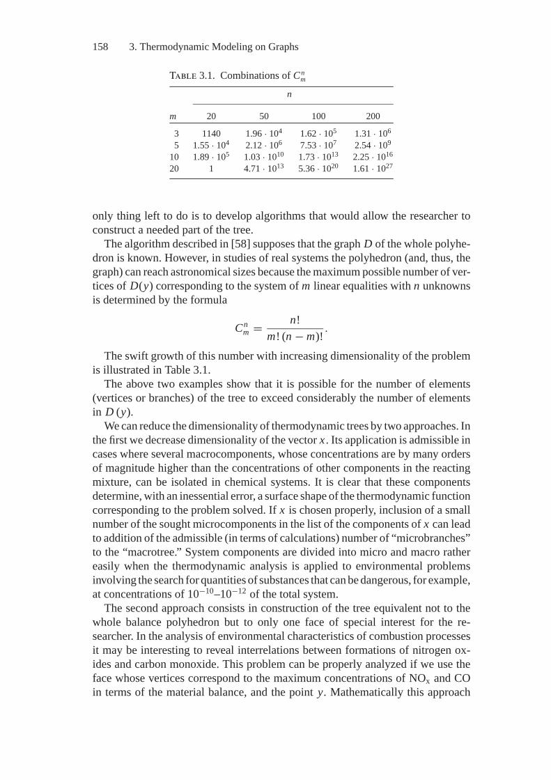
158 3. Thermodynamic Modeling on Graphs
Table 3.1. Combinations of Cnm
n
m 20 50 100 200
3 1140 1.96 · 104 1.62 · 105 1.31 · 106
5 1.55 · 104 2.12 · 106 7.53 · 107 2.54 · 109
10 1.89 · 105 1.03 · 1010 1.73 · 1013 2.25 · 1016
20 1 4.71 · 1013 5.36 · 1020 1.61 · 1027
only thing left to do is to develop algorithms that would allow the researcher toconstruct a needed part of the tree.
The algorithm described in [58] supposes that the graph D of the whole polyhe-dron is known. However, in studies of real systems the polyhedron (and, thus, thegraph) can reach astronomical sizes because the maximum possible number of ver-tices of D(y) corresponding to the system of m linear equalities with n unknownsis determined by the formula
Cnm = n!
m! (n − m)! .
The swift growth of this number with increasing dimensionality of the problemis illustrated in Table 3.1.
The above two examples show that it is possible for the number of elements(vertices or branches) of the tree to exceed considerably the number of elementsin D (y).
We can reduce the dimensionality of thermodynamic trees by two approaches. Inthe first we decrease dimensionality of the vector x . Its application is admissible incases where several macrocomponents, whose concentrations are by many ordersof magnitude higher than the concentrations of other components in the reactingmixture, can be isolated in chemical systems. It is clear that these componentsdetermine, with an inessential error, a surface shape of the thermodynamic functioncorresponding to the problem solved. If x is chosen properly, inclusion of a smallnumber of the sought microcomponents in the list of the components of x can leadto addition of the admissible (in terms of calculations) number of “microbranches”to the “macrotree.” System components are divided into micro and macro rathereasily when the thermodynamic analysis is applied to environmental problemsinvolving the search for quantities of substances that can be dangerous, for example,at concentrations of 10−10–10−12 of the total system.
The second approach consists in construction of the tree equivalent not to thewhole balance polyhedron but to only one face of special interest for the re-searcher. In the analysis of environmental characteristics of combustion processesit may be interesting to reveal interrelations between formations of nitrogen ox-ides and carbon monoxide. This problem can be properly analyzed if we use theface whose vertices correspond to the maximum concentrations of NOx and COin terms of the material balance, and the point y. Mathematically this approach
3.3. Thermodynamic Interpretations of Hydraulic Circuit Theory 159
is equivalent to the first one, since the polyhedron face can be treated as a poly-hedron corresponding to the reduced dimensionality of the space of variables.When we construct flat two-dimensional faces, an approach that is convenientfrom the standpoint of graphical interpretation of the problem solved, in orderto choose a list of the vector x components, we should apparently apply therelation
n = m + 2,
where n is the dimensionality of x , and m is the number of linear material balances.With the efficient application of both approaches the algorithm presented in
[58] may also be admissible in terms of calculation time. Of course, it doesnot mean that the search for new effective algorithms for constructing thermo-dynamic trees is not advisable. Irrespective of the success in these efforts thetheoretical value of the “idea of tree” is unquestioned. A sketch variant of thealgorithm of tree construction on the basis of the second approach is discussed inSection 4.4.
3.3. Thermodynamic Interpretations ofHydraulic Circuit Theory
Historical BackgroundRelations between thermodynamics and hydrodynamics, and hence hydraulic cir-cuit theory, since the latter can be handled as part of the hydrodynamics from thestandpoint of physics, were considered in Section 1.3.
The methods of loop flows (currents) and nodal pressures (potentials) are knownto be basic in describing flow (current) distribution. In so far as they are analogs ofthe methods of cycles and potentials in the thermodynamics, they emerged almostsimultaneously with the latter (the methods of cycles and loop currents are sug-gested by Clausius and Kirchhoff; the methods of potentials in the thermodynamicsand the circuit theory are suggested by Gibbs and Maxwell). Kirchhoff [108] andMaxwell [129] who are the founders of the theory of electric circuits, showed thepossibility for transition from their methods to extreme models. In [129] Maxwellalso established mathematical equivalence of the methods of potentials and loopcurrents.
Both the method of loop currents, whose mathematical prerequisite is the equal-ity to zero of the integral over a closed loop, and the method of potentials are onlyapplicable to studying equilibrium systems that can be defined as “conservative”(∮
d f = 0) and as “potential” (see Chapter 1). Note that Euler was the first tointroduce, in 1765, the potential function into hydrodynamics and physics as awhole.
Section 1.3 of the book has already presented equilibrium interpretations of thelaws of motion of electric charges (Ohm’s law) and viscous liquid (the Darcy–Weisbach law). In addition we recall here an equilibrium nature of the classical

160 3. Thermodynamic Modeling on Graphs
system of hydrodynamics equations:∂ρ
∂τ+ div (ρw) = 0, (3.2)
ρ dwdt = ρF − ∇ P + (η + ζ ) ∇divw + η�w, (3.3)
cpρdTdτ
− d Pdτ
= q + div (χ∇T )
+{
ζ (divw)2 + 2η
[(∂wx
∂x
)2+
(∂wy
∂y
)2+
(∂wz
∂z
)2]
+η
[(∂wx
∂y+ ∂wy
∂x
)2+
(∂wx
∂z+ ∂wz
∂x
)2+
(∂wy
∂z+ ∂wz
∂y
)2]}
,
(3.4)
P = f1 (ρ, T ) , S = f2 (ρ, T ) , (3.5)
where ρ is density; τ is time; w is velocity; F is volumetric force; η, ζ arecoefficients of dynamic and volumetric viscosity; cp is specific heat capac-ity at constant pressure; q is the heat quantity supplied to a unit volume ina unit time due to nonmechanical reasons; and χ is a coefficient of thermalconductivity.
Equation (3.2) describes a flow continuity condition. The Navier-Stokes equa-tion (3.3) is an extension of Newton’s second law to moving liquid. Equation (3.4)formulates the energy conservation law. Relations (3.5) are the thermal and caloricstate equations, respectively. Inclusion of the state equations into system (3.2)–(3.5) implies application of the assumption on the equilibrium thermodynamicnature of liquids dynamics.
In the 1960s V.Ya. Khasilev extended the main statements of electric circuitstheory developed in late 19th century, applying them to multiloop hydraulic cir-cuits. The equilibrium nature of the liquid flow equations proves the validity ofsuch an extension. In the basic works on hydraulic circuit theory [104–107, 132,130] V.Ya. Khasilev made a comparative analysis of computational properties forthe methods of loop flow rates and nodal pressures, and he suggested extrememethods (MP) for solving HCT problems. He outlined thereby two directions inMP application: 1) calculations of flow distribution and 2) technical and economicoptimization of hydraulic networks. In the first case the objective function formwas determined from the Kirchhoff-Maxwell heat theorem on least heat productionin a passive circuit [130].
V.Ya. Khasilev showed the impact of closing relations (relations between thepressure losses and the flow rates in circuit branches) on mathematical features ofthe optimization problems of circuit schemes and parameters (namely, convexityor concavity of the objective function and its slight slope near the extremum point)[104, 106]. In their book, A.P. Merenkov and V.Ya. Khasilev [130] studied theserelations mainly in terms of the accuracy of flow distribution calculations.
3.3. Thermodynamic Interpretations of Hydraulic Circuit Theory 161
A.P. Merenkov and N.N. Novitsky performed a rather detailed analysis of theinverse flow distribution problems [132, 130, 134].
O.A. Balyshev extended the HCT principles to the analysis of nonstationaryflow distribution in networks [16–18]. From the joint solution of the equations ofcontinuity, Navier–Stokes, and state, he obtained formulas of closing relations formotion of media with constant density and media subject to the equation of statefor the ideal gas (or real gas with constant compressibility).
B.M. Kaganovich formulated the problems of thermodynamic interpretation ofHCT and study of heterogeneous hydraulic circuits, i.e., circuits with a complexphase and chemical composition of flows [85, 91].
Fundamentals of Hydraulic Circuit TheoryThe cited work [130] presents two definitions of hydraulic circuits (HCs). Accord-ing to the first definition, HCs represent an aggregate of conductors intended fortransportation of liquids. The second defines HC as a mathematical model con-sisting of two constituents: a calculated scheme in the form of the directed graph[180]; and algebraic relations describing flow of liquids (gases) along graph’s arcs.The present book applies only the second definition as the most adequate to itspurposes.
HCT studies direct and inverse problems of flow distribution in hydraulic circuitsand problems of the optimal synthesis (choice of the schemes and parameters) ofcircuits. The latter are usually related to the technical and economic optimizationof pipeline networks (water, heat, oil and gas supply, etc.).
For real objects HCT has studied three key types of models up to now:
1) circuits with lumped parameters, in which the resistances of branches (grapharcs) and effective heads are independent of flow distribution;
2) circuits with variable (regulated) parameters, in which at least part of the branchcharacteristics (effective heads, heads and sinks (sources) at nodes, etc.) arethe functions of sought quantities, and determined (“regulated”) by the flowdistribution itself;
3) circuits with distributed parameters, in which the characteristics of branches(resistances, effective heads) alter depending on distances to the nodes adjacentto the corresponding branch.
If all relationships for the branches of a distributed or regulated circuit arerepresented as a differentiable function of no more than two variables (for example,length and time or length and temperature), then the closing relations for themmay be written in a “lumped” integral form, at least theoretically. At the same timethe holonomy of the Pfaffian forms makes the thermodynamic representation ofhydrodynamic relationships feasible.
For each mentioned model, the circuit branches are divided into active (withsources of effective heads: pumps, compressors, gravity, wind pressure, etc.) andpassive (without such sources). By the graph theory the circuit scheme (part of the
162 3. Thermodynamic Modeling on Graphs
scheme) without closed loops is called a tree and the branches supplementing thetree to the closed (cyclic) scheme are called chords.
Application of the thermodynamics concepts in HCT calls for expansion of theaccepted classifications of models and the system of notions. Open and closed,homogeneous and heterogeneous circuits naturally supplement the classification.The open circuits have sources and sinks: As do any other open thermodynamicsystems, they exchange substance with the environment. In the closed circuitssources and sinks are absent.
There are two approaches to division of hydraulic circuits into homogeneous(uniform) and heterogeneous (nonuniform) types. In thermodynamics the hetero-geneous systems include those in which a substance is present in different phases.Based on thermodynamic terminology we can assume conditionally that the flowsin different circuit branches subject to different closing relations (e.g., flows corre-sponding to turbulent and laminar flow modes) belong to different phases. There-fore, the circuits with the distinct relationships between head losses and flows inthe branches can be considered heterogeneous. This classification of circuits wassuggested in [81].
In this context, the book addresses basically heterogeneous circuits, ones inwhich flows in separate branches contain several phases. In general, such flowsare the vectors whose components are the flows of different chemical substancesin different phase states on the branch.
For circuits with lumped parameters the problems of stationary flow distributioncalculation are described in [130] in three ways: a) on the basis of the loop systemof equations; b) using nodal potentials; c) in the extreme statement on the basis ofthe minimum heat production theorem.
The loop system of equations has the form:
Ax = Q, (3.6)Bh = B H, (3.7)hi = fi (xi ) , i = 1, . . . , n, (3.8)
where x and xi are a vector of flows in the circuit branches and its i th component,respectively; A = [aij] is an (m − 1) × n-matrix of connections of independentnodes to branches; aij = 1, if the flow in the i th branch runs to the j th node inaccordance with the specified direction; aij = −1, if the i th flow runs from the j thnode and aij = 0 if j does not belong to branch i ; Q is a vector of external sourcesand sinks at the nodes
m∑i=1
Q j = 0;
m is the number of nodes; n is the number of branches; h and hi are a vector ofhead losses and its i th component, respectively; H is a vector of effective heads;B = [bki ] is an c × n-matrix of the coincidences of loops and branches; bij = 1 ifthe initially specified direction of flow in the branch coincides with the specified
3.3. Thermodynamic Interpretations of Hydraulic Circuit Theory 163
direction of loop encircling; bij = −1 when these directions are opposite; bij = 0when the i th branch is not included in loop k.
The matrix equation (3.6) describes the first Kirchhoff law, which expressesthe requirement of mass conservation in the flows of liquid for hydraulic circuits.Equation (3.7) formulates the second Kirchhoff law, which may be interpreted asthe extension of the general energy conservation principle to separate circuit loops.Expression (3.8) is a closing relation.
For the method of nodal potentials equation (3.7) in system (3.6)–(3.8) is sub-stituted by the equation
h − H = AT P, (3.9)
where AT − [aij] is an m × n complete transposed matrix of connections of nodesto branches; P is a vector of nodal pressures.
The extreme principle of flow distribution in circuits as based on the works byKirchhoff and Maxwell is formulated in [130] as the heat theorem. It means thatflows in the open passive circuit are distributed so that they produce a minimumamount of heat. The corresponding mathematical problem is formulated in thiscase as the following:
Find
min∑
ihi xi (3.10)
subject toAx = Q,
hi = fi (xi ) , i = 1, . . . , n.
The authors of [130] also studied the possible extension of the theorem aboutleast thermal effect on active circuits, in particular with different exponents β inthe closing relations (see below). This was done by such variation of the objectivefunction type that the solution to the extreme problem coincided with the solutionto the system of equations (3.6)–(3.8). As a result the following function wasdetermined:
F (x) =n∑
i=1
(fi (xi ) xi
1 + β− Hi xi
). (3.11)
In [78] it is shown that this formula can be derived directly from the Lagrangeprinciple of virtual work. Actually for hydraulic circuits this principle is inter-preted as follows. If the flow distribution in the circuit is equilibrium, i.e., theequilibrium of all forces exerted on a moving medium (pressure, friction, gravity,etc.) is observed in every section of every branch, the work done on any infinites-imal deviation of flows in the branches from their equilibrium values equals zero.Mathematically, this principle is interpreted as follows:
dL = zi xβ
i dxi − Hidxi = 0, i = 1, . . . , n, (3.12)
where zi is the resistance of the i th branch.
164 3. Thermodynamic Modeling on Graphs
Obviously equation (3.12) represents an extremum condition of the objectivefunction (3.11) and reveals its physical sense. F (x) is the variation of energy ofthe total flow in the circuit at its deviation from the optimal (equilibrium) value(the Lagrange function). It is clear that the principle of virtual work allows an easydetermination of the extremality criterion for passive circuits (H = 0).
The closing relations fi (xi ) for incompressible liquids for the HCT problemsin [92] are represented in two forms:
hi = fi (xi ) = zi xβ
i , (3.13)hi = zi1xi + zi2x2
i . (3.14)These relations can be applied to model characteristics of the sources of effective
heads by the equationH = H 0 − zinxβ
in, (3.15)in which the second term on the right-hand side is a head loss in an imaginarybranch simulating the internal resistance of a pump.
The formulas to determine z from the Darcy–Weisbach equation and exper-imental relations for the friction coefficient λ were studied in [132] from thecomputational standpoint.
V.Ya. Khasilev [104, 106] and, later, B.M. Kaganovich [76] examined the effectof type of closing relations on the mathematical properties of problems pertain-ing to technical and economic optimization of hydraulic circuits. V.Ya. Khasilevperformed the analysis on the basis of the following formula of pipeline diame-ter that was derived from the elementary transformation of the Darcy–Weisbachequation
d = axψ h−ϕ,
Where a, ψ and ϕ are coefficients. For turbulent flow (β = 2) ψ ≈ 0.38 andϕ ≈ 0.19.
Assume, for an objective function that indicates some cost characteristic of thenetwork, that the function’s term are proportional to di in the problem of technicaland economic optimization; in the case of 1 ≤ β ≤ 2 this function proves to beconvex by the axes hi and concave by xi . In the extremum point h here it will becharacterized by the exceptionally slight slope (the small curvature). The doublingof head loss in comparison to optimal value increases the liquid transportation costby 4.6 , and a twofold decrease in the loss leads to just a 3.8 cost increase. Someadjustments in the results of analysis made by V.Ya. Khasilev were performedin [76] in terms of constraints on the conditions of network development andupgrading.
The methods of network optimization and solutions to direct and inverse prob-lems of flow distribution that were developed in HCT are presented in detail in[130]. On the whole, hydraulic circuit theory has been applied extensively forseveral decades to solve engineering problems of development and operation ofpipeline, and of other hydraulic networks with flows homogeneous in their chem-ical and phase compositions.
3.3. Thermodynamic Interpretations of Hydraulic Circuit Theory 165
Models of Nonstationary Flow DistributionO.A. Balyshev extended HCT principles to the analysis of nonstationary flowdistribution in multiloop hydraulic systems using the premises of the “equilibriumdynamics” [16–18]. In the context of our discussion his results are of interest as thebasis for thermodynamic studies on nonstationary processes in complex hydraulicnetworks. Application of the thermodynamic analysis to the hydraulic shock in aseparate pipe was demonstrated in Section 1.3.
The laws of mass and energy conservation, as is customary in HCT, were writtenby O.A. Balyshev in the circuit (Kirchhoff) form, and closing relation type wasdetermined by transforming the Navier–Stokes and state equations.
For the circuits with lumped parameters, O.A. Balyshev’s model has the form
Ax (τ ) = Q (τ ) , (3.17)Bh (τ ) = B H (τ ) , (3.18)
hi = fi (xi (τ )) , i = 1, . . . , n. (3.19)
In the simplest case, when each i th flow of incompressible liquid experiencesonly forces of inertia, pressure and friction, the form of the functions fi is deter-mined from the initial Navier–Stokes equation
ρdw
dτ= −d P
dl− λ
ρw2
2d, (3.20)
or fromdx (τ )
dτ= −πd2
4d Pdl
− 2λx2 (τ )πd3ρ
(3.21)
when we pass from velocity w to mass flow x .From here we have the differential closing relation
−dP = 8λx2 (τ )π2d5ρ
dl + 4πd2
dx (τ )dτ
dl. (3.22)
Introduction of the notion of instantaneous head (pressure) drop
hi = Pi (0, τ ) − Pi (li , τ ) , (3.23)
will lead to
hi = 8λx2i (τ )
π2d5ρl + 4
πd2dxi (τ )
dτl (3.24)
or
hi (τ ) = fi (xi (τ )) = zi1x2i (τ ) + zi2
dxi (τ )dτ
. (3.25)
Model (3.17)–(3.19) enriched the hydraulic circuit theory in terms of opportu-nities it affored to analysis of network stability to variations in the vectors H , Qand Z , and to optimization of operation conditions.
166 3. Thermodynamic Modeling on Graphs
Thermodynamic ModelsWe seek to determine a type of the objective function for an extreme thermody-namic flow distribution model for a closed active circuit with lumped parametersand isothermal liquid flow. In such a function the entropy production in the i thbranch will be represented by the relation
�Si = �qi T −1 = hi xi T −1, (3.26)
which is based on the assumption on the equalities
Ti = Tenv = T, i = 1, . . . , n,
where the index “env” refers to the environment. Entropy production in the circuitas a whole is
�Scir = 1T
∑i
hi xi . (3.27)
The same amount of entropy is transferred to the environment and its accumu-lation there leads to the increase in entropy of an isolated system (the circuit plusthe environment), given as
�Sis = 1T
∑i
hi xi . (3.28)
Hence, for the considered system the function value∑i
hi xi .
should be maximal. Then the following model becomes obvious:Find
max∑
ihi xi (3.29)
subject to
Ax = 0, (3.30)∑i
Hi xi − ∑i
hi xi = 0, (3.31)
hi = fi (xi ) , i = 1, . . . , n. (3.32)
The right-hand side of the first Kirhchhoff law equation (3.30) is equal to zerodue to the absence of sources and sinks (Q = 0) in the closed system. Equa-tion (3.31) is the balance of produced and consumed energy in the circuit. Thesigns are chosen from the condition of thermodynamics that the removed heat(∑i
hi xi ) be negative.
If the closing relation is determined by expression (3.13), model (3.29)–(3.32)takes the following form:
3.3. Thermodynamic Interpretations of Hydraulic Circuit Theory 167
Find
max∑
izi xβ +1
i (3.33)
subject to
Ax = 0, (3.34)∑i
Hi xi − ∑i
zi xβ +1i = 0, (3.35)
hi = zi xβ
i , i = 1, . . . , n. (3.36)
Comparison between (3.33) and (3.35) reveals the possibility of replacing theobjective function (3.31) by the expression
max∑
iHi xi (3.37)
and then formulating the following statement: The flows in a closed active hy-draulic circuit are distributed so that the energy produced by sources of effec-tive heads and, correspondingly, the energy consumed is maximal. This state-ment provides information about the physical regularities of flow distribution incircuits, in addition to information of the theorem concerning the least thermalaction.
To analyze mathematical properties of model (3.33)–(3.36) we will write theLagrange function of the circuit, representing preliminarily condition (3.34) in theform ∑
i∈I j
ai j xi = 0, j = 1, . . . , m − 1, (3.38)
where I j is a subset of branches incident to node j .Then the Lagrange function will be
L =n∑
i=1zi xβ+1
i −m−1∑j=1
λ j∑i∈I j
a ji xi + λm
(n∑
i=1zi xβ+1
i −n∑
i=1Hi xi
), (3.39)
where λ j and λm are Lagrange multipliers.Let us take the derivative of (3.39) with respect to xi and equate it to zero:
(β + 1) (λm + 1) zi xβ
i + λbi − λei − λm Hi = 0, (3.40)
where λbi and λei are multipliers for the initial and final nodes of branch I , respec-tively.
Since, at Hi = 0,
λbi − λei = (β + 1) (λm + 1) zi xβ
i = (β + 1) (λm + 1) hi , (3.41)
the difference of the Lagrange multipliers for nodes incident to the i th branch isproportional to the head loss in it.
The analytical expression for λm is obtained by addition of the derivatives∂L
/∂xi for all i belonging to any closed loop k with effective heads. The sum will
168 3. Thermodynamic Modeling on Graphs
have the form
(β+1) (λm + 1)∑i∈k
hi − λm∑i∈k
Hi = (β + 1) (λm + 1)∑i∈k
Hi − λm∑i∈k
Hi = 0.
(3.42)(Equality to zero is explained by the equilibrium character of flow distribution).
Expression (3.42) does not contain λ j , since “+λ j ” and “−λ j ” vanish for eachnode j . From (3.42) it follows that
λm = − (β + 1)β
. (3.43)
As β > 0, then |λm | > 1. For the linear closing relation (β = 2), λm = −2,and for the quadratic relation (β = 2), λm = −1.5. Since the multiplier λm is aderivative of the entropy with respect to the energy imbalance, its negativity isquite clear. If we could increase the energy of flows
∑i Hi xi without an increase
of its consumption∑
i zi xβ+1i and entropy production, then with respect to the
equilibrium state ∑i
Hi xi =∑
izi xβ+1
i and S = max S
S of the system should have decreased.Substituting (3.43) into (3.40) we will find that in a general case
λbi − λei = �λi = λm (Hi − hi ) . (3.44)
Depending on the choice of the m − 1 independent nodes the absolute valuesof λ j ( j �= m) will vary, but the �λi will remain unchanged.
The second partial derivatives of L with respect to xi are
∂2L∂x2
i= β (β + 1) (λm + 1) zi xβ−1
i ≤ 0,
since λm < −1. Hence, the solution to problem (3.33)–(3.36) corresponds to themaximum of L = f (x) and the maximum of the objective function (3.33) for anadmissible set of solutions. Fig. 3.3a illustrates the possibility of a maximiu pointto exist for the convex objective function. The objective function a′b′ that has themaximum Fmax is an intersection of the vertical surface drawn through a nonlinearadmissible region of solutions to the problem (the region ab), perpendicular to theplane x1x2, with the surface of the function f (x) above this plane.
An open active circuit (with internal sources of effective heads and externalsources and sinks) represents a thermodynamic system, whose conditions for in-teraction with the environment are determined by fixing enthalpy and pressure. Infact, the setting of the vector of nodal flows at fixed circuit resistance uniquelydetermines pressure (head) differentials between the points of sources and sinks,and between the energy flows as well. For both these and isolated systems, themaximum entropy is achieved at the equilibrium state. In this case the model offlow distribution takes the following form:
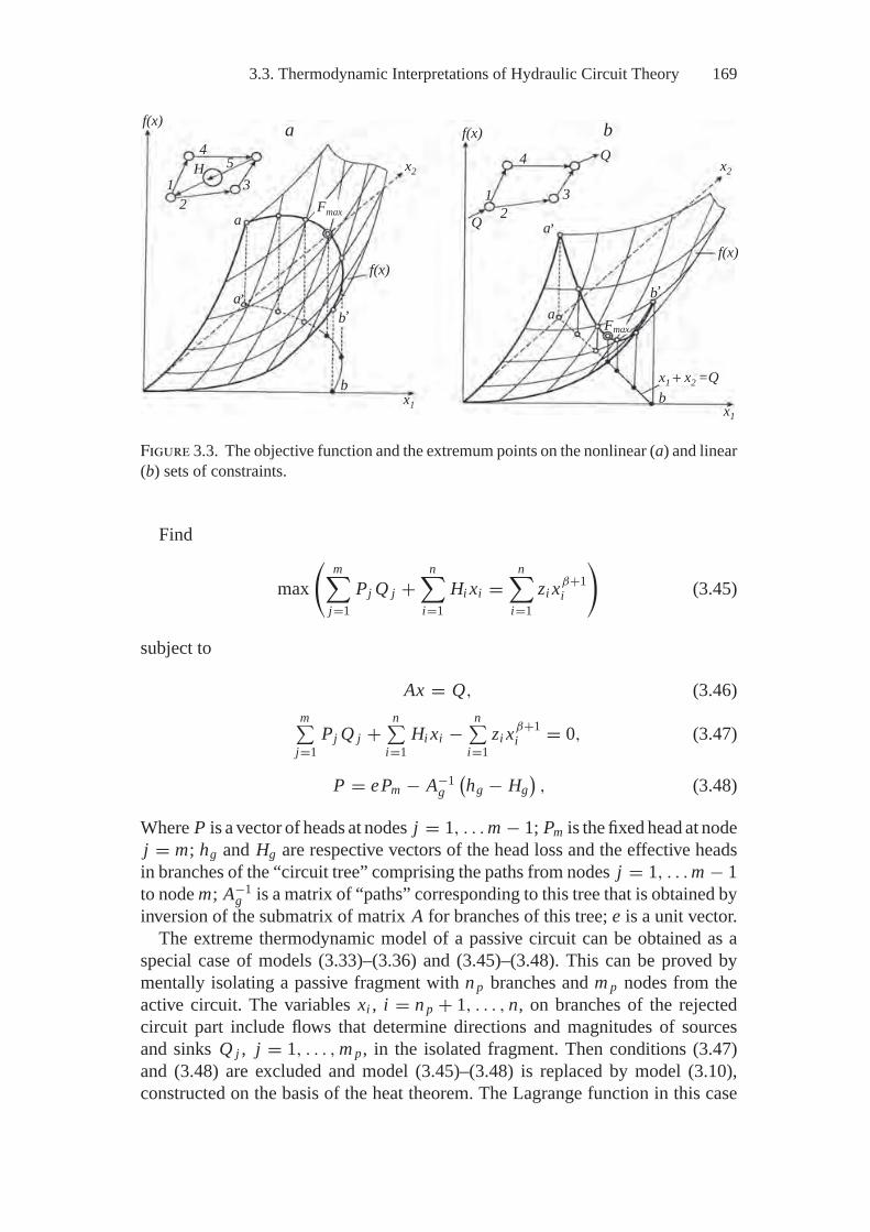
3.3. Thermodynamic Interpretations of Hydraulic Circuit Theory 169
f(x)
44
32
1
Q
5H1
23
f(x)
f(x)a b
a
x2 x2
b
x1 + x2 =Q
a,
b,
f(x)
Q
a
x1
b
a,
x1
Fmax
b,
Fmax
Figure 3.3. The objective function and the extremum points on the nonlinear (a) and linear(b) sets of constraints.
Find
max(
m∑j=1
Pj Q j +n∑
i=1Hi xi =
n∑i=1
zi xβ+1i
)(3.45)
subject to
Ax = Q, (3.46)m∑
j=1Pj Q j +
n∑i=1
Hi xi −n∑
i=1zi xβ+1
i = 0, (3.47)
P = ePm − A−1g
(hg − Hg
), (3.48)
Where P is a vector of heads at nodes j = 1, . . . m − 1; Pm is the fixed head at nodej = m; hg and Hg are respective vectors of the head loss and the effective headsin branches of the “circuit tree” comprising the paths from nodes j = 1, . . . m − 1to node m; A−1
g is a matrix of “paths” corresponding to this tree that is obtained byinversion of the submatrix of matrix A for branches of this tree; e is a unit vector.
The extreme thermodynamic model of a passive circuit can be obtained as aspecial case of models (3.33)–(3.36) and (3.45)–(3.48). This can be proved bymentally isolating a passive fragment with n p branches and m p nodes from theactive circuit. The variables xi , i = n p + 1, . . . , n, on branches of the rejectedcircuit part include flows that determine directions and magnitudes of sourcesand sinks Q j , j = 1, . . . , m p, in the isolated fragment. Then conditions (3.47)and (3.48) are excluded and model (3.45)–(3.48) is replaced by model (3.10),constructed on the basis of the heat theorem. The Lagrange function in this case
170 3. Thermodynamic Modeling on Graphs
has the form
L =n p∑
i=1zi xβ+1
i −m−1∑j=1
λ j
(∑i∈I j
a ji xi
)
and its second derivatives are∂2L∂x2
i= β (β + 1) zi xβ−1
i ≥ 0. (3.49)
Hence, the extremum of L (x) is the point of minimum, and thus the problemof entropy maximization is transformed to the problem of heat minimization, andthe Kirchhoff–Maxwell theorem is deduced as a corollary of the second thermo-dynamics law with its extension to passive circuits. Coincidence of the form ofobjective functions in the “entropy” models (3.33)–(3.36) and (3.45)–(3.48) withthe “energy” model (3.10) is due to the fact that the multiplier 1
/T is removed
from the maximized expression (3.10) on the assumption of constant temperature.The revealed interrelation of flow distribution problems is a special case of the
general thermodynamic law. It states that systems with constant energy tend tomaximum entropy, and in systems in which fixation of any parameters resultsin energy exchange with the environment, the minimum of the correspondingenergy kind is achieved. In the considered case of fixed flows of liquid (gas),which the circuit exchanges with its environment, we minimize mechanical energyconsumption or, what is the same, quantity of heat liberated in the circuit.
Fig. 3.3a and b presents a graphical interpretation of the transformation ofmaximization problem to the minimization problem for the objective function thatis convex on the unlimited set of variables.
Here we will not discuss thermodynamic interpretations of the models withregulated and distributed parameters that were considered in [81]. It should onlybe pointed out that such models can often be reduced to models with lumpedparameters, as was explained above.
At the end of our discussion of homogeneous circuits let us show that theextremality criterion (3.11) that was justified above using the principle of virtualworks, can be obtained from thermodynamic model (3.33)–(3.36). To do this weperform elementary transformations of the partial Lagrange function:
L =n∑
i=1zi xβ+1
i + λm
(n∑
i=1zi xβ+1
i −n∑
i=1Hi xi
)
= −∑
i
β + 1β
(zi xβ+1
iβ + 1 − Hi xi
)= const
∑i
(fi (xi ) xi
β + 1 − Hi xi
).
Of course, the constant may be removed from the extremality criterion.The analysis presented in this section and the previous portion of the book show
that extreme models of homogeneous circuits can be constructed on the basis oftwo competitors: a) the second law of thermodynamics and the principle of virtualworks to describe stationary (or nonstationary, if the time variable is excluded from
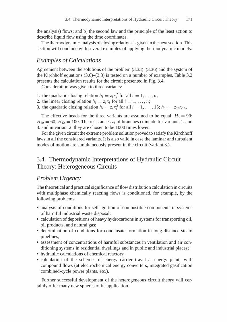
3.4. Thermodynamic Interpretations of Hydraulic Circuit Theory 171
the analysis) flows; and b) the second law and the principle of the least action todescribe liquid flow using the time coordinates.
The thermodynamic analysis of closing relations is given in the next section. Thissection will conclude with several examples of applying thermodynamic models.
Examples of CalculationsAgreement between the solutions of the problem (3.33)–(3.36) and the system ofthe Kirchhoff equations (3.6)–(3.8) is tested on a number of examples. Table 3.2presents the calculation results for the circuit presented in Fig. 3.4.
Consideration was given to three variants:
1. the quadratic closing relation hi = zi x2i for all i = 1, . . . , n;
2. the linear closing relation hi = zi xi for all i = 1, . . . , n;3. the quadratic closing relation hi = zi x2
i for all i = 1, . . . , 15; h16 = z16x16.
The effective heads for the three variants are assumed to be equal: H5 = 90;H10 = 60; H12 = 100. The resistances zi of branches coincide for variants 1. and3. and in variant 2. they are chosen to be 1000 times lower.
For the given circuit the extreme problem solution proved to satisfy the Kirchhofflaws in all the considered variants. It is also valid in case the laminar and turbulentmodes of motion are simultaneously present in the circuit (variant 3.).
3.4. Thermodynamic Interpretations of Hydraulic CircuitTheory: Heterogeneous Circuits
Problem UrgencyThe theoretical and practical significance of flow distribution calculation in circuitswith multiphase chemically reacting flows is conditioned, for example, by thefollowing problems:� analysis of conditions for self-ignition of combustible components in systems
of harmful industrial waste disposal;� calculation of depositions of heavy hydrocarbons in systems for transporting oil,
oil products, and natural gas;� determination of conditions for condensate formation in long-distance steam
pipelines;� assessment of concentrations of harmful substances in ventilation and air con-
ditioning systems in residential dwellings and in public and industrial places;� hydraulic calculations of chemical reactors;� calculation of the schemes of energy carrier travel at energy plants with
compound flows (at electrochemical energy converters, integrated gasificationcombined-cycle power plants, etc.).
Further successful development of the heterogeneous circuit theory will cer-tainly offer many new spheres of its application.
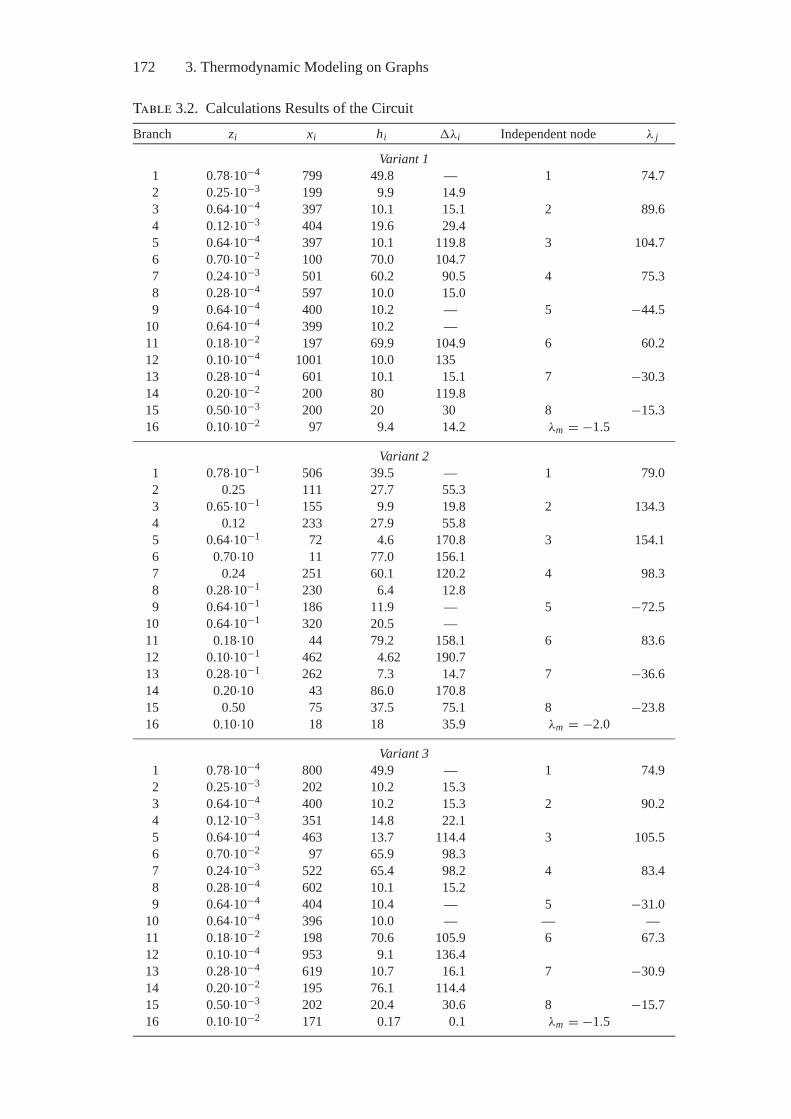
172 3. Thermodynamic Modeling on Graphs
Table 3.2. Calculations Results of the CircuitBranch zi xi hi �λi Independent node λ j
Variant 11 0.78·10−4 799 49.8 — 1 74.72 0.25·10−3 199 9.9 14.93 0.64·10−4 397 10.1 15.1 2 89.64 0.12·10−3 404 19.6 29.45 0.64·10−4 397 10.1 119.8 3 104.76 0.70·10−2 100 70.0 104.77 0.24·10−3 501 60.2 90.5 4 75.38 0.28·10−4 597 10.0 15.09 0.64·10−4 400 10.2 — 5 −44.5
10 0.64·10−4 399 10.2 —11 0.18·10−2 197 69.9 104.9 6 60.212 0.10·10−4 1001 10.0 13513 0.28·10−4 601 10.1 15.1 7 −30.314 0.20·10−2 200 80 119.815 0.50·10−3 200 20 30 8 −15.316 0.10·10−2 97 9.4 14.2 λm = −1.5
Variant 21 0.78·10−1 506 39.5 — 1 79.02 0.25 111 27.7 55.33 0.65·10−1 155 9.9 19.8 2 134.34 0.12 233 27.9 55.85 0.64·10−1 72 4.6 170.8 3 154.16 0.70·10 11 77.0 156.17 0.24 251 60.1 120.2 4 98.38 0.28·10−1 230 6.4 12.89 0.64·10−1 186 11.9 — 5 −72.5
10 0.64·10−1 320 20.5 —11 0.18·10 44 79.2 158.1 6 83.612 0.10·10−1 462 4.62 190.713 0.28·10−1 262 7.3 14.7 7 −36.614 0.20·10 43 86.0 170.815 0.50 75 37.5 75.1 8 −23.816 0.10·10 18 18 35.9 λm = −2.0
Variant 31 0.78·10−4 800 49.9 — 1 74.92 0.25·10−3 202 10.2 15.33 0.64·10−4 400 10.2 15.3 2 90.24 0.12·10−3 351 14.8 22.15 0.64·10−4 463 13.7 114.4 3 105.56 0.70·10−2 97 65.9 98.37 0.24·10−3 522 65.4 98.2 4 83.48 0.28·10−4 602 10.1 15.29 0.64·10−4 404 10.4 — 5 −31.0
10 0.64·10−4 396 10.0 — — —11 0.18·10−2 198 70.6 105.9 6 67.312 0.10·10−4 953 9.1 136.413 0.28·10−4 619 10.7 16.1 7 −30.914 0.20·10−2 195 76.1 114.415 0.50·10−3 202 20.4 30.6 8 −15.716 0.10·10−2 171 0.17 0.1 λm = −1.5
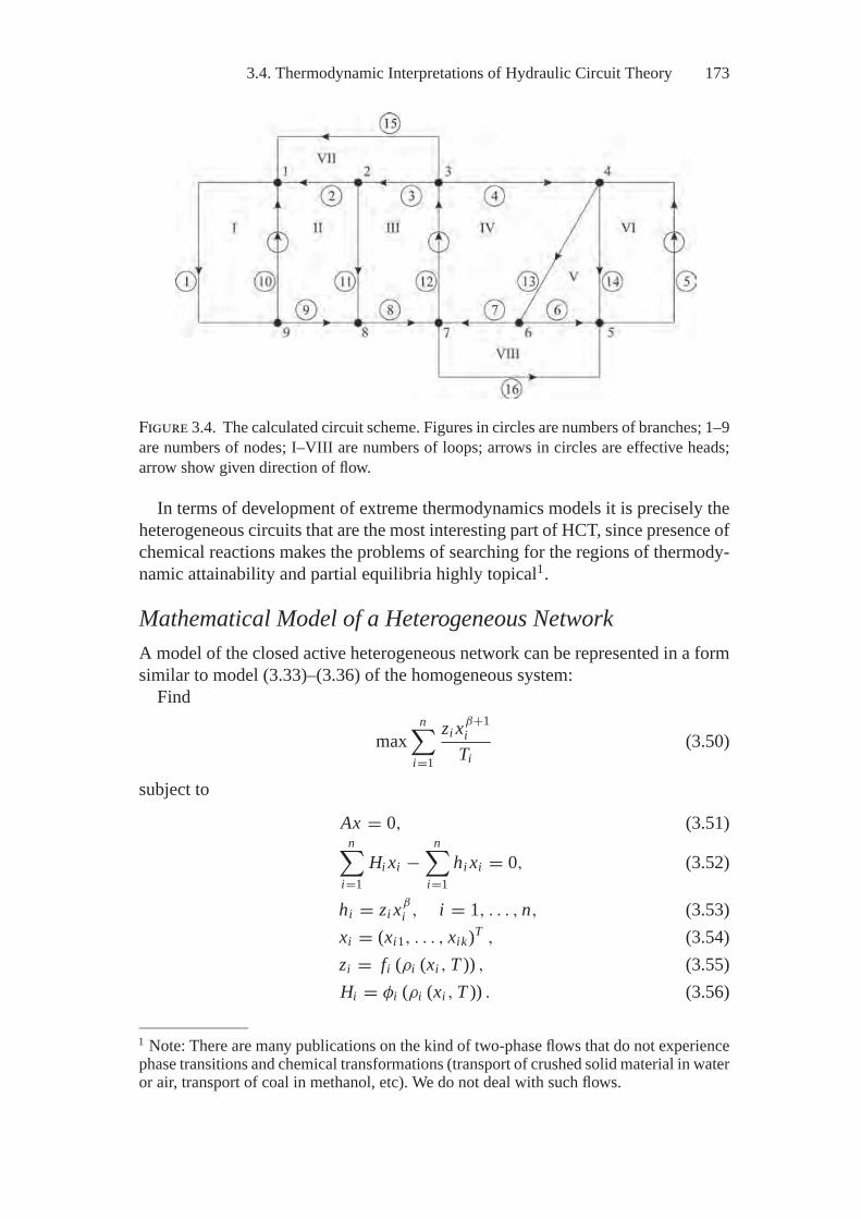
3.4. Thermodynamic Interpretations of Hydraulic Circuit Theory 173
Figure 3.4. The calculated circuit scheme. Figures in circles are numbers of branches; 1–9are numbers of nodes; I–VIII are numbers of loops; arrows in circles are effective heads;arrow show given direction of flow.
In terms of development of extreme thermodynamics models it is precisely theheterogeneous circuits that are the most interesting part of HCT, since presence ofchemical reactions makes the problems of searching for the regions of thermody-namic attainability and partial equilibria highly topical1.
Mathematical Model of a Heterogeneous NetworkA model of the closed active heterogeneous network can be represented in a formsimilar to model (3.33)–(3.36) of the homogeneous system:
Find
maxn∑
i=1
zi xβ+1i
Ti(3.50)
subject to
Ax = 0, (3.51)n∑
i=1Hi xi −
n∑i=1
hi xi = 0, (3.52)
hi = zi xβ
i , i = 1, . . . , n, (3.53)xi = (xi1, . . . , xik)T , (3.54)zi = fi (ρi (xi , T )) , (3.55)Hi = φi (ρi (xi , T )) . (3.56)
1 Note: There are many publications on the kind of two-phase flows that do not experiencephase transitions and chemical transformations (transport of crushed solid material in wateror air, transport of coal in methanol, etc). We do not deal with such flows.
174 3. Thermodynamic Modeling on Graphs
The functional dependences (3.53) and (3.56) indicate that the heterogeneouscircuits belong to the models with distributed parameters. In order to revealproperties of system (3.50)–(3.56) and possibilities of its reduction (approxi-mation) to the model with lumped parameters, first, one must study the char-acter of the closing relations (3.53). Such a study is the major subject of thissection.
Thermodynamic Analysis of Closing RelationsAvailability of physically and mathematically valid closing relations makes it pos-sible to conduct a qualitative physical and mathematical analysis of diverse het-erogeneous circuits. For example, these closing relations enable one to determineconditions for occurrence of multiphase flows, possible changes in the type ofpiezometric plots (graphical relationships between head loss and branch length)at chemical transformations and phase transitions, reasons for the many-valuedsolutions to a flow distribution problem, and so on.
When we derived the closing relations for multicomponent and multiphaseflows, we took as the basis premise the equilibrium between different phases,which, in turn, is determined by the equality of chemical and other potentials.
Originally the idea of thermodynamic analysis of relationships between headlosses and flow was tested on the example of a homogeneous isothermal flow ofincompressible liquid. We considered the phase equilibrium between two condi-tional flows: a turbulent tube and an annular laminar layer surrounding it: Thetwo move uniformly and in the same direction relative to one another. Thus, thetrue picture of vortex formation and increase in the flow turbulence degree withthe growth of flow velocity was substituted by an imaginary picture of continuousgrowth of the turbulent tube diameter dt from zero to d. The authors borrowed theidea of conditional flows from Landau’s theory of quantum liquids [120], in whichLandau used the concept of conditional superfluid and normal flow.
Since the studied flows are homogeneous and isothermal, we naturally reducedthe equality of chemical potentials to the equality of hydraulic potentials, namelypressures, and correspondingly, to the equality of pressure losses in the turbulenttube (�Pt ) and the laminar flow (�Pl) between any two tube cross-sections.The value of �Pt was calculated by the Darcy–Weisbach formula (1.55) and theSchifrinson formula was applied to determine the friction coefficient
λt = 0.11(k/
dt)0.25
, (3.57)
where k is a roughness coefficient.When �Pl was determined by (1.55), the equivalent diameter dl of the laminar
ring and the coefficient λl were calculated from the expressions [3]:
dl = 4ω
h= 4
π(d2 − d2
t)
4π (d + dt )= d − dt , (3.58)
λl = ARe
= 96ν
w (d − dt ), (3.59)
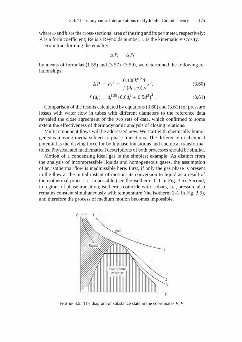
3.4. Thermodynamic Interpretations of Hydraulic Circuit Theory 175
where ω and h are the cross-sectional area of the ring and its perimeter, respectively;A is a form coefficient; Re is a Reynolds number; ν is the kinematic viscosity.
From transforming the equality
�Pt = �Pl
by means of formulas (1.55) and (3.57)–(3.59), we determined the following re-lationships:
�P = zx2 = 0.108k0.25lf (dt (w)) ρ
x2, (3.60)
f (dt ) = d1.25t
(0.6d2
t + 0.5d2)2. (3.61)
Comparison of the results calculated by equations (3.60) and (3.61) for pressurelosses with water flow in tubes with different diameters to the reference datarevealed the close agreement of the two sets of data, which confirmed to someextent the effectiveness of thermodynamic analysis of closing relations.
Multicomponent flows will be addressed now. We start with chemically homo-geneous moving media subject to phase transitions. The difference in chemicalpotential is the driving force for both phase transitions and chemical transforma-tions. Physical and mathematical descriptions of both processes should be similar.
Motion of a condensing ideal gas is the simplest example. As distinct fromthe analysis of incompressible liquids and homogeneous gases, the assumptionof an isothermal flow is inadmissible here. First, if only the gas phase is presentin the flow at the initial instant of motion, its conversion to liquid as a result ofthe isothermal process is impossible (see the isotherm 1–1 in Fig. 3.5). Second,in regions of phase transition, isotherms coincide with isobars, i.e., pressure alsoremains constant simultaneously with temperature (the isotherm 2–2 in Fig. 3.5),and therefore the process of medium motion becomes impossible.
Figure 3.5. The diagram of substance state in the coordinates P, V.
176 3. Thermodynamic Modeling on Graphs
Therefore, the flow was assumed to be polytropic. For ideal gases the polytropeequation has the form
PV γ = const. (3.62)
For the adiabatic process we have
γ = cp
cυ
, (3.63)
where cp and cυ are the isobaric and isochoric heat capacities, respectively. Whenγ tends to unity, the process is isothermal at its limit.
The next supposition was that the moving medium represents a spatially homo-geneous mixture of gas and suspended fog droplets.
Density of such a medium is determined from the expression
ρ = x(x − xc) ρ−1
g + xcρ−1c
, (3.64)
where x is the mass flow; and the indices c and g refer to condensed and gas phases,respectivetly.
Since at moderately high flow pressures
ρg << ρc,
equation (3.64) can be replaced by the approximate expression
ρ = ρgx(x − xc) . (3.65)
The closing relation for the polytropic flow of condensing ideal gas (the flowof the condensed phase at the initial cross-section of tube is equal to zero) can bedetermined from the Darcy–Weisbach equation written in the differential form
−d P = λρw2
2ddl. (3.66)
To substitute the variable w by the mass flow x we will express the density ρ atan arbitrary flow cross-section via the density ρ1 at the initial state.
From the polytrope equation (3.62) follows
ρg = ρg1
(PP1
)1/γ, (3.67)
since ρ = 1/υ.
In terms of (3.65) we have
ρ = ρ1
(PP1
)1/γ x(x − xc) . (3.68)
Since
x = 0.25wρπd2,
3.4. Thermodynamic Interpretations of Hydraulic Circuit Theory 177
then
−d P = 8λP1/γ1 x (x − xc)
π2ρ1d5 P1/γ dl. (3.69)
Let us introduce the notation
ψ = 8λP1/γ1
π2d5ρ1. (3.70)
ThenP1∫
P2
P1/γ d P =l∫
0
ψx (x − xc) dl
and
P (γ+1)/γ1 − P (γ+1)/γ
2 = ϕx (x − xc) l, (3.71)
where
ϕ = ψ(γ + 1)
γ. (3.72)
Expression (3.71) is an integral form of the closing relation for the “ideal”two-phase flow from which the final pressure is determined:
P2 =(
P (γ+1)/γ1 − ϕx (x − xc) l
)γ /(γ+1). (3.73)
The closing relation for the single-phase flow (xc = 0) is derived as a particularcase of (3.71), namely,
P (γ+1)/γ1 − P (γ+1)/γ
2 = ϕx2l, (3.74)
and at γ = 1 it transfers to the known formula for the isothermal gas flow,
P21 − P2
2 = ϕx2l. (3.75)
At the same time equation (3.71) is not symmetric relative to phase transitions:gas → liquid; and liquid → gas. When the gas phase flow rate (x = xc) is equal tozero, the pressure loss in the branch also turns to zero, which is certainly incorrecttheoretically. This property of the determined closing relation is quite clear, as itwas derived by the ideal gas state equation. But in principle this equation is notadequate for the description of condensed phases. However, when the gas phasedisappears in the flow the errors in determination of pressure losses by equation(3.71) are practically negligible. This is due to the fact that the condensate densityat a distance from the critical point is much higher than the gas density, and thevalue of �P sharply decreases with condensation. If the tube diameter were chosenwith the proviso that a single-phase gas flow passed through it, then, with motionof the same condensate mass in it, �P would approach zero.
Let us mention an easily comprehensible fact, namely, that the phase transitions(and the chemical transformations) can lead to both convex (Fig. 3.6, curve 3)
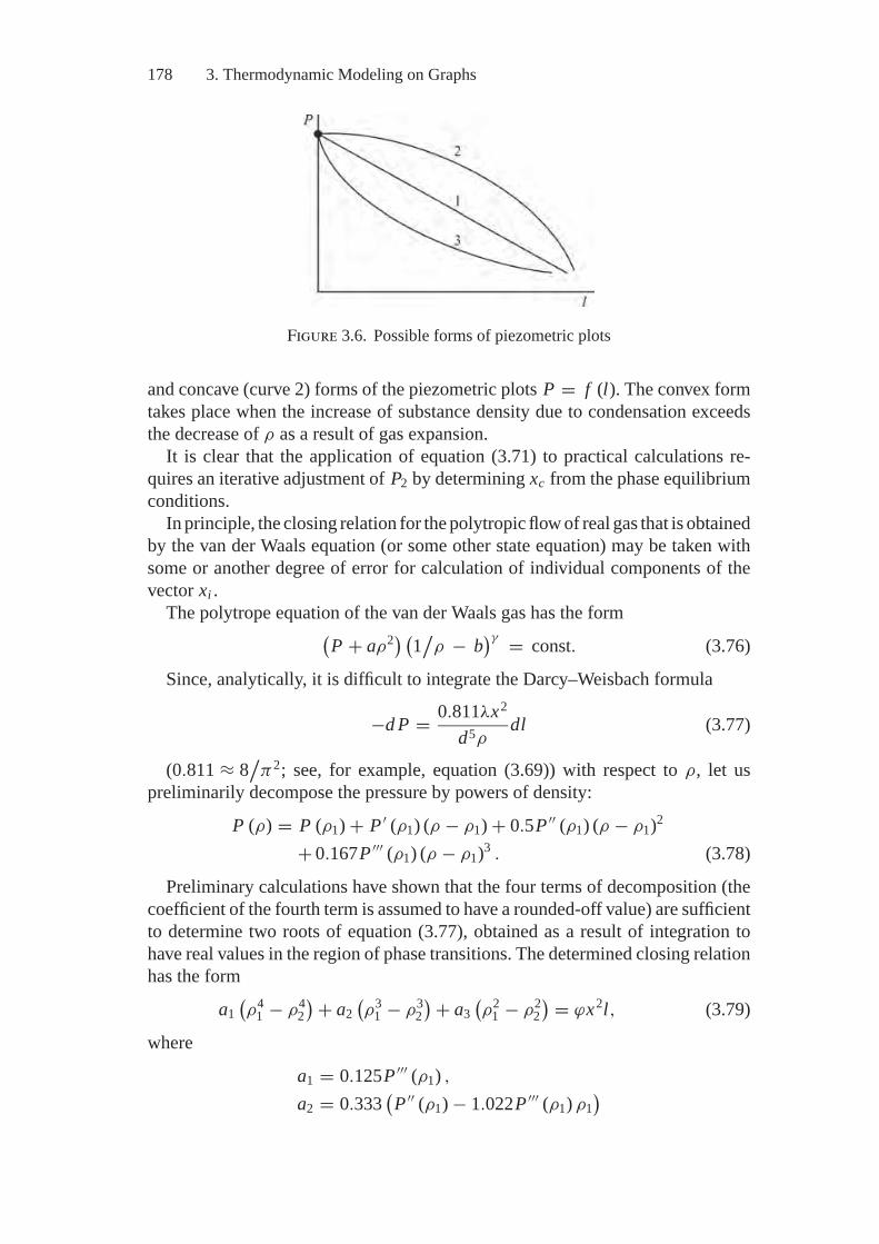
178 3. Thermodynamic Modeling on Graphs
Figure 3.6. Possible forms of piezometric plots
and concave (curve 2) forms of the piezometric plots P = f (l). The convex formtakes place when the increase of substance density due to condensation exceedsthe decrease of ρ as a result of gas expansion.
It is clear that the application of equation (3.71) to practical calculations re-quires an iterative adjustment of P2 by determining xc from the phase equilibriumconditions.
In principle, the closing relation for the polytropic flow of real gas that is obtainedby the van der Waals equation (or some other state equation) may be taken withsome or another degree of error for calculation of individual components of thevector xi .
The polytrope equation of the van der Waals gas has the form(P + aρ2) (1/ρ − b
)γ = const. (3.76)
Since, analytically, it is difficult to integrate the Darcy–Weisbach formula
−d P = 0.811λx2
d5ρdl (3.77)
(0.811 ≈ 8/π2; see, for example, equation (3.69)) with respect to ρ, let us
preliminarily decompose the pressure by powers of density:
P (ρ) = P (ρ1) + P ′ (ρ1) (ρ − ρ1) + 0.5P ′′ (ρ1) (ρ − ρ1)2
+ 0.167P ′′′ (ρ1) (ρ − ρ1)3 . (3.78)
Preliminary calculations have shown that the four terms of decomposition (thecoefficient of the fourth term is assumed to have a rounded-off value) are sufficientto determine two roots of equation (3.77), obtained as a result of integration tohave real values in the region of phase transitions. The determined closing relationhas the form
a1(ρ4
1 − ρ42) + a2
(ρ3
1 − ρ32) + a3
(ρ2
1 − ρ22) = ϕx2l, (3.79)
where
a1 = 0.125P ′′′ (ρ1) ,
a2 = 0.333(P ′′ (ρ1) − 1.022P ′′′ (ρ1) ρ1
)
3.4. Thermodynamic Interpretations of Hydraulic Circuit Theory 179
and
a3 = 0.5(P ′ (ρ1) − P ′′ (ρ1) ρ1 + 0.501P ′′′ (ρ1) ρ2
1).
It is obvious that for the single-phase flow of ideal gas the second and thirdderivatives of pressure with respect to density turn out to be zero and equation(3.79) converts to the quadratic relation (3.75).
It is of no doubt that the terms of no lower than the third power should bepresent in the algebraically expressed closing relations for any flows experiencingphase transitions. Indeed, the region of phase transitions in the state diagrams liesbelow the critical point, at which the first and second derivatives of pressure withrespect to the volume (density) equal zero. This point can be determined only bythe equations in which two first derivatives do not vanish identically.
Analytical dependences between pressure loss and flow for chemically reactingflows can be determined only at the limiting idealization of the studied process. Tohave a clear picture of chemical transformation influence on liquid flow we shouldalso exclude from mathematical description of the problem all factors that are notdirectly related to transformations of substances (e.g., changes in medium densitywith variation in temperature and pressure).
Based on the indicated requirements we will consider an isothermal flow of twoliquid incompressible isomers 1 and 2 as a model example. In the flow the firstcomponent is converted to the second as a result of a monomolecular reaction ofthe first order, i.e., a reaction corresponding to the equation,
dx1
dτ= −kx1, (3.80)
where x1 is a mole fraction of component 1, and k is a rate constant of the reaction.In this case the flow density ρ is determined by the equation
ρ =(( 1
ρ2− 1
ρ1
)x2 + 1
ρ1
)−1, (3.81)
x2 is calculated from the material balance equation
x1 + x2 = 1, (3.81a)
and the solution to equation (3.80) is
x1 = e−kτ , (3.82)
which is true provided that for τ = 0, x1 = 1 and x2 = 0,
x2 = 1 − e−kτ . (3.83)
In terms of (3.83), equation (3.81) can be transformed as
ρ =( 1
ρ2+
( 1ρ1
− 1ρ2
)e−kτ
)−1. (3.84)
180 3. Thermodynamic Modeling on Graphs
If the form of the function ρ = f (τ ) is known, the relationships between �Pand x can be found from the Darcy–Weisbach equation
−dP = λw2 (ρ) ρ (τ )2d
dl (ρ (τ )) = 8λx2
π2d5ρ (τ )dl (ρ (τ )) . (3.85)
Integration of (3.85) results in
�P = 32λx3
π3d7
[τ
ρ22
+ 2kρ2
( 1ρ1
− 1ρ2
) (1 − e−kτ
) + 12k( 1
ρ1− 1
ρ2
)2 (1 − e−2kτ
)]. (3.86)
Expression (3.86) represents the dependence of pressure loss on the time ofliquid motion between the pipeline section that is taken as initial and the currentsection. However, before passing to the thermodynamic analysis the variable τ
should be excluded, i.e., it is necessary to find a relation between �P and x at thefixed l that is revealed for the flows with phase transitions. To solve this problem,first the form of the function l = f (τ ) is determined:
dl = w (ρ (τ )) dτ,
l = 4xπd2
[τ
ρ22
+ 1k
( 1ρ1
− 1ρ2
) (1 − e−kτ
)]. (3.87)
Then a simple transformation of equation (3.86) is performed:
�P = 32λx3
π3d7
[τ
ρ22
+ 1kρ2
( 1ρ1
− 1ρ2
) (1 − e−kτ
)]
+ 32λx3
π3d7
[ 1kρ2
( 1ρ1
− 1ρ2
) (1 − e−kτ
) + 12k
×( 1
ρ1− 1
ρ2
)2 (1 − e−2kτ
)]. (3.88)
Comparison of (3.87) and (3.88) clearly shows that pressure loss �P can berepresented as the sum of the term depending on l and the one independent of l:
�P = ϕx2l (τ )ρ2
+ [ψ1
(1 − e−kτ
) + ψ2(1 − e−2kτ
)]x3. (3.89)
The first term on the right-hand side of (3.89) coincides with classical expres-sions of closing relations for circuits with lumped parameters, provided the pipelength and the time for the liquid to pass through it are fixed and the liquid densityequals the density of the second isomer (the final reaction product). The secondterm is a correction for the value of �P that is determined by the change in densityof the moving medium because of the chemical reaction.
Equation (3.89) shows that when τ and l are equal to zero, �P also vanishes.At τ → ∞ the relationship �P = f (l) tends to become linear. This conclusion is
3.4. Thermodynamic Interpretations of Hydraulic Circuit Theory 181
clear, since the chemical transformations are completed in an infinitely long timeperiod and the density becomes constant. The sign of “chemical” correction forthe variation in �P depends on the sign of difference 1
/ρ1 − 1
/ρ2, i.e., on the
density variation during reaction. If the density of the final product ρ2 exceeds ρ1,then �P = f (l) on the initial branch section is concave. At ρ2 < ρ1 the function�P (l) becomes convex. The function P (l) = P1 − �P (l) is naturally convexwhen ρ2 > ρ1 and concave at ρ2 < ρ1 (see Fig. 3.6).
Note that both the “chemical” and “phase” corrections are cubic (or higher-power) functions of the flow. This fact can be explained physically, since theimpact of chemical transformations on hydrodynamics is similar to the im-pact of phase transitions and is determined solely by the change in the flow-ing medium density (if the possible variation in viscosity is neglected). There-fore, the mathematical descriptions of the effects of these processes on liquid(gas) flow should also be similar. The impossibility of applying closing rela-tions of a power lower than the third power for flows with a variable phasecomposition was shown above. The same is naturally true of chemically reactingliquids.
Based on what is said above, let us represent the closing relation (3.89) in a“more thermodynamic” form, excluding from it the time variable that is uniquelyrelated with ρ1, ρ2 and l at the fixed x :
�P = ϕ1 (ρ2, l) x2 + ϕ2 (ρ1, ρ2) x3. (3.90)
For the strict derivation of expressions (3.89) and (3.90) we introduced very se-vere constraints into the initial problem statement. It is clear, however, that the areaof qualitative analysis using the obtained equations can be considerably extendedin comparison with the area formally corresponding to the accepted mathematicalmodel. Thus, the initial and final compositions of flows can be assumed to benot pure substances, but mixtures and equation (3.81a) in a general form can besupposed to describe a linear material balance. For the flows with ρ = f (P, T ) itis natural to assume that the right-hand side of equation (3.90) represents only thetwo first terms of a more complicated relation that probably includes terms of apowers higher than the third with respect to x .
The obtained closing relations can be applied to show that at least at k << 1,the property of “cost function slight slope along the head axes” that was es-tablished by V.Ya. Khasilev, does not change essentially at a transition fromthe flows of incompressible media to the chemically reacting flows (see Sec-tion 3.3). Indeed, with the indicated constraint on the reaction rate constant,time τ during which the liquid passes the distance l is expressed approximatelyby
τ ≈ constd2
x,
and the dependence �P = f (x) becomes close to quadratic, which was assumedby V.Ya. Khasilev. It may be supposed that at certain constraints the properties of
182 3. Thermodynamic Modeling on Graphs
cost functions of pipeline networks that were determined in [76, 106] hold for themultiphase flows as well.
A fundamental character of closing relations (availability of a “lumped” com-ponent of the second power and corrections of higher powers) will apparently notchange at a transition from complete to partial equilibria in flows. However, acomplex analytical type of these relations indicates that in practical calculationsof heterogeneous circuits they should be either determined by the iterative com-putational procedures or indirectly accounted for at approximation of the modelsof hydraulic systems on the whole (see below).
In concluding the analysis of closing relations, we will briefly address theirderivation for nonsteady flow distribution. The analysis can be based on equation(3.25). The terms of its right-hand side are naturally interpreted as the stationary(the first term) and the nonstationary (the second term) components of head losses.
It is obvious that when we study a steady process, the second term turns out tobe equal to zero and equation (3.25) reduces to the traditional form of the closingrelation (3.13). Certainly, if the change in the “steady form” for the flows withphase transitions and chemical transformations is taken into account, it seemsnatural to replace (3.25) by the more general expression
hi (τ ) = fi (xi , τ ) + ψidxi (τ )
dτ, (3.91)
where the form of terms on the right-hand side is determined by the properties ofthe moving medium (gas, heterogeneous mixture of gas and condensed particles)and the character of processes running in the flows (phase transitions, chemicalreactions, friction, heat exchange, etc.).
The problem of determining the expression for the first term was tackled to aconsiderable extent above. The problem of searching for the second term formwill be not discussed in this book. It should be a subject of independent extensivestudies. It should be noted, only, that depending on the disturbance nature thederivative dxi (τ )
/dτ in (3.91) may be substituted by the derivative of pressure or
temperature, the sum of derivatives of individual components of the vector flow inbranch i , and so on.
On the whole the thermodynamic analysis of nonsteady flow distribution provesto be useful, when we are interested in the results of transient processes rather thanin the time of their occurrence, which was considered above. For example, in theanalysis of impact of the fast operation of stop valves in a pipeline network, it isimportant to determine a maximum liquid pressure and to check whether it exceedsan admissible value or not. The question the matter of what fraction of a second orof what seconds such pressure arises—is not so important (if, of course, the choiceof the maximum rate of stop valve operation is not dealt with). In the studies ofprocesses of heavy hydrocarbons, precipitation in gas and oil pipelines, or soot intubes of chemical reactors, thermodynamics helps determine maximum precipi-tation of harmful substances relative to hourly mass flow of the moving mediumand then estimate tentatively the time of tube “overgrowing.” At least in a numberof cases it is more important to determine the probability that explosive mixtures
3.4. Thermodynamic Interpretations of Hydraulic Circuit Theory 183
are formed in communications of energy or other industrial plants than to find thetime taken for the corresponding reactions to proceed under favorable conditions.
Examples of Heterogeneous Circuit ApplicationThe methods of constructing thermodynamic models of heterogeneous hydraulicsystems to solve applied problems will be illustrated by two examples: 1) firespread in complex air exchange systems; and 2) burning and disposal of harmfulpollutants of industrial plants.
Prior to direct modeling of fire spread we will briefly address the topical problemof analysis of normal operation conditions for air exchange systems. This subjectwas touched upon in [91].
Ventilation and air conditioning systems for residential and industrial premisesshould provide both the requisite sanitary standards in temperature and moistureand the acceptable chemical composition of air. Whereas until recently the mainmethod of controlling harmful emissions on premises was the intensive dilution ofindoor air with outdoor air, now such a purification method may be dangerous. Thisis because in the “purifying” outdoor air the concentrations of harmful substancesmay be much higher than the (admissible) standards. Since indoor and outdoortemperature and moisture usually differ considerably, chemical composition ofair flows in any building changes significantly. These changes can be calculatedby modeling the air exchange systems on the basis of heterogeneous hydrauliccircuits.
Modeling of fires in air exchange systems is the most sophisticated and theo-retically interesting case when we attempt a “chemical and hydraulic” descriptionof the system. Such systems include ventilation networks of buildings and otherstructures (such as mines and subways). The appropriate models, if available,will supposedly contribute to working out preventive measures and improving firecontrol.
The mathematical modeling of fires has been the subject of numerous publica-tions (see, for example, [66]). Originality of the authors’ approach consists in thenetwork problem statement and its presentation in terms of HCT and thermody-namics.
Prior to solution of such a complex problem currently we can create just a draftmodel that should be adjusted successively in the course of further studies.
To make the presentation clear we will first describe fires on the basis of a loopsystem of hydraulic circuit equations that is similar to system (3.6)–(3.8) and applyit in combination with MEIS; then we will show how to pass from this system tonodal potentials and the extreme model (3.50)–(3.56).
We will not construct equivalent calculated schemes of a real object, and wewill suppose that the air exchange scheme (hydraulic circuit) is known. A simplestopen double-loop hydraulic circuit is chosen as an example (Fig. 3.7a). Assumethat the fire occurs on branch 2 and can spread to the rest of the scheme. Thedifference in densities on individual circuit branches induces gravitational headsdenoted by Hg1 and Hg2.
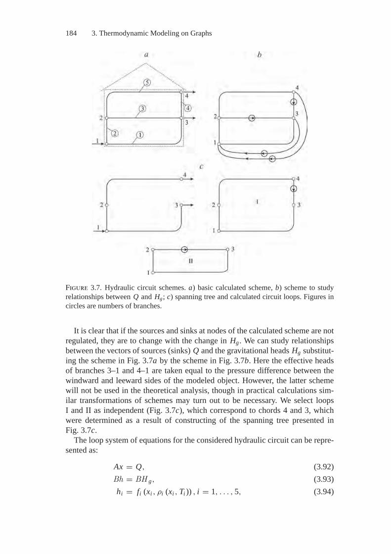
184 3. Thermodynamic Modeling on Graphs
Figure 3.7. Hydraulic circuit schemes. a) basic calculated scheme, b) scheme to studyrelationships between Q and Hg; c) spanning tree and calculated circuit loops. Figures incircles are numbers of branches.
It is clear that if the sources and sinks at nodes of the calculated scheme are notregulated, they are to change with the change in Hg . We can study relationshipsbetween the vectors of sources (sinks) Q and the gravitational heads Hg substitut-ing the scheme in Fig. 3.7a by the scheme in Fig. 3.7b. Here the effective headsof branches 3–1 and 4–1 are taken equal to the pressure difference between thewindward and leeward sides of the modeled object. However, the latter schemewill not be used in the theoretical analysis, though in practical calculations sim-ilar transformations of schemes may turn out to be necessary. We select loopsI and II as independent (Fig. 3.7c), which correspond to chords 4 and 3, whichwere determined as a result of constructing of the spanning tree presented inFig. 3.7c.
The loop system of equations for the considered hydraulic circuit can be repre-sented as:
Ax = Q, (3.92)Bh = BH g, (3.93)hi = fi (xi , ρi (xi , Ti )) , i = 1, . . . , 5, (3.94)
3.4. Thermodynamic Interpretations of Hydraulic Circuit Theory 185
Hgk = fk(zk, �ρk
), k = 1, 2, (3.95)
Ti = Ti (�T ) , �Ti = Tbi − Tei = ϕi (αi , Fi , Tenv) , (3.96)xi = (xi1, . . . , xie)T = ψi (y, Ti , Pi ) , (3.97)
where Hg is a vector of the gravitational heads; zk and �ρk are, respectively,the difference of geodetic level marks and the difference of densities of the up-ward and downward flows in the kth loop; Tbi and Tei are temperatures at theinlet and the outlet of the i th branch; Tenv is an environmental temperature; αiand Fi are the heat transfer coefficient and the heat exchange surface on the i thbranch.
A natural idea of computational algorithms is to construct a circuit model withlumped parameters (3.6)–(3.8) for iterative calculations instead of model (3.92)–(3.97) to adjust the values of components in the vectors xi and Hg at each iteration.
It seems reasonable to calculate “normal” (before the fire) flow distribution at thefirst iteration, then to calculate fire on branch 2 and adjust chemical composition,gravitational heads, averaged temperatures, and densities of the moving medium.There are several variants for choosing the model for determination of combustionresults, e.g.: 1) stoichiometric description of a small number of basic reactions;2) determination on MEIS of the final equilibrium point xeq at the given vector y,the given list of the components x and the fixed enthalpy H and pressure P; 3)MEIS application to search for xext with the same data, as in the second variant,and the setting of the objective function that is the sum of concentrations of themost dangerous substances.
The first stoichiometric variant is the least suitable for assessing fire impact.However, successive sophistication of the considered model and determinationof relationships between the mathematical properties and the assumptions madewill make it possible to apply the stoichiometric model. Expediency of using thethird model (the main block of MEIS – xext) is due at least to the fact that weare interested in both the fire spread over the circuit branches and the spread ofharmful substances beyond its direct zone that can cause poisoning of people atcertain concentrations.
Gravitational heads at the first approximation can be determined by the simplestrelation
Hgk = zk (ρck − ρhk) , (3.98)
where ρck and ρhk are the average densities of the upward and downward flows inthe kth loop, respectively. They are given by
ρck = 1zk
∑i∈Ick
ρi zi , ρhk = 1zk
∑i∈Ihk
ρi zi , (3.99)
where ρi and zi are the average density and the difference of marks along thevertical axis for the i th branch, respectively; Ick and Ihk are sets of branches withthe downward (ck) and upward (hk) flows.
186 3. Thermodynamic Modeling on Graphs
Temperatures of the branches and their variations can also be determined thelinear approximation from the equations:
qi = αi Fi (Ti − Tenv) τ, Ti = 0.5 (Tbi + Tei ) , (3.100)qi = ci xi (Tbi − Tei ) τ, (3.101)
where qi are heat losses to the environment on the i th branch, and ci is the spe-cific heat of the multicomponent flow. The estimated time τ corresponding to thesupposedly dangerous rate of fire spread should be varied, apparently, to analyzereal objects. In terms of the construction principles of thermodynamic models, τ
does not belong to the variables sought in the problem.In addition, the heat balance equations for the circuit as a whole should be
satisfied:
AbCbTb − AeCeTe = ACT = q, (3.102)
where Ab and Ae are submatrices of the complete m × n matrix A of connec-tions of all circuit nodes and branches that fix separately the initial “b” and thefinal “e” nodes of the branches; Cb = [cbi ] and Ce = [cei ] are diagonal matri-ces of the heat capacity magnitudes of the medium flowing to the initial node ofbranch i (cbi ) and out of the final node of the same branch (cei ) ; C = [c] is adiagonal matrix of the average heat capacities of flows; Tb, Te, and T are vectorsof the temperatures at the initial and the final nodes and on the circuit branches,respectively; and q is a vector of external heat sources and sinks at the circuitnodes.
When adjusting ρi , we determine the density ρiθ of every θ th component ofthe i th flow from the thermodynamic equation of state, and calculate the total flowdensity by the relation
ρi =∑θ
ρθ i xθ∑θ
xθ
, (3.103)
where xθ is the mole quantity of the θ th component.At the second and following iterations, system (3.6)–(3.8) is calculated with the
adjusted values of Hg and ρ. In this case, if for some branch, Ti happens to exceedthe ignition temperature T f l of the moving medium, the flame characteristics for itare determined by MEIS (or the stoichiometric model) and then the circuit param-eters are adjusted by the algorithm applied at the first iteration. The calculationsterminate, if the difference in the values of xi (or some other variables) at twosuccessive iterations does not exceed a given small value ε.
If the model of fires is constructed on the basis of the method of nodal potentials,equation (3.93) is replaced by the expression
h − Hg = AT P (x) . (3.104)
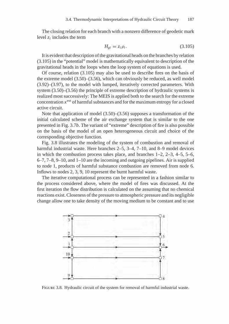
3.4. Thermodynamic Interpretations of Hydraulic Circuit Theory 187
The closing relation for each branch with a nonzero difference of geodetic marklevel zi includes the term
Hgi = ziρi . (3.105)
It is evident that description of the gravitational heads on the branches by relation(3.105) in the “potential” model is mathematically equivalent to description of thegravitational heads in the loops when the loop system of equations is used.
Of course, relation (3.105) may also be used to describe fires on the basis ofthe extreme model (3.50)–(3.56), which can obviously be reduced, as well model(3.92)–(3.97), to the model with lumped, iteratively corrected parameters. Withsystem (3.50)–(3.56) the principle of extreme description of hydraulic systems isrealized most successively: The MEIS is applied both to the search for the extremeconcentration xext of harmful substances and for the maximum entropy for a closedactive circuit.
Note that application of model (3.50)–(3.56) supposes a transformation of theinitial calculated scheme of the air exchange system that is similar to the onepresented in Fig. 3.7b. The variant of “extreme” description of fire is also possibleon the basis of the model of an open heterogeneous circuit and choice of thecorresponding objective function.
Fig. 3.8 illustrates the modeling of the system of combustion and removal ofharmful industrial waste. Here branches 2–5, 3–4, 7–10, and 8–9 model devicesin which the combustion process takes place, and branches 1–2, 2–3, 4–5, 5–6,6–7, 7–8, 9–10, and 1–10 are the incoming and outgoing pipelines. Air is suppliedto node 1, products of harmful substance combustion are removed from node 6.Inflows to nodes 2, 3, 9, 10 represent the burnt harmful waste.
The iterative computational process can be represented in a fashion similar tothe process considered above, where the model of fires was discussed. At thefirst iteration the flow distribution is calculated on the assuming that no chemicalreactions exist. Closeness of the pressure to atmospheric pressure and its negligiblechange allow one to take density of the moving medium to be constant and to use
Figure 3.8. Hydraulic circuit of the system for removal of harmful industrial waste.

188 3. Thermodynamic Modeling on Graphs
the circuit with lumped parameters. The MEIS-based information on the flow ofair and harmful substances through the combustion devices is applied to calculatea combustion process and to adjust density of the moving medium on branches2–5, 3–4, 7–10, 8–9, 4–5, and 7–8; then, according to the rules of flows mixing,the same is done on branches 5–6 and 6–7. Further, the calculations are repeatediteratively, until the differences in values of the vector x components at a transitionfrom the kth to the (k + 1)th iteration become lower than the given small value ε.From the result of the computational process it can be determined, for example,if the products of incomplete combustion are formed at individual combustiondevices because of air shortage, and if incomplete combustion leads to appearanceof explosive mixtures in the outgoing pipelines.
4Methods and Algorithms of Searchingfor Thermodynamic Equilibria
A small boy asked the mathematician: “How much is twice two?” The mathematiciansaid that he would think and after three days of thinking he shared his joy with theboy: “I have proved that this problem has a solution!”
A joke
4.1. E.G. Antsiferov’s General Two-Stage Techniqueof Searching for Extreme Concentrations
As was noted in Section 2.4, even if we managed to strictly prove reducibility ofthe problem solved by MEIS to the convex programming (CP) problem, the diffi-culties caused by the setting of constraints on monotone change of thermodynamicfunctions presented in implicit form remain. E.G. Antsiferov [4, 7, 8] suggesteda two-stage technique of searching for the vector of extreme concentrations xext.According to his idea, the surface of the thermodynamic function level that con-tains the point xext is determined at the first stage, coordinates of this point aresought on this surface at the second stage.
The first stage is based on the analysis of possible locations of the point xext inthe thermodynamic attainability region Dt (y) relative to the points y and xeq. Thisstage was described in Section 2.4 (see Fig. 2.9).
Different cases are considered in the search for extreme concentration point xext.The first situation is the case of monotone decrease of Gibbs energy (or anothercharacteristic function) on the interval segment [y, xmat]. In this case the secondstage is excluded (Fig. 2.9a), since the point xmat proves to be a solution to theproblem of searching for xext. The first stage reduces to solution of the canonicallinear programming (LP) problem (nonlinear thermodynamic constraints do notinfluence the location of xext).
The second situation is the case of continuous increase of the function G(x) onthe segment y, xmat (Fig. 2.9b). In this case the canonical CP problem (2.116) issolved at the second stage.
The third situation is the case of the minimum point of G(x) (the thermodynamic“pothole”) on the segment [y, xmat] (Fig. 2.9c). This point is taken as the sought
189
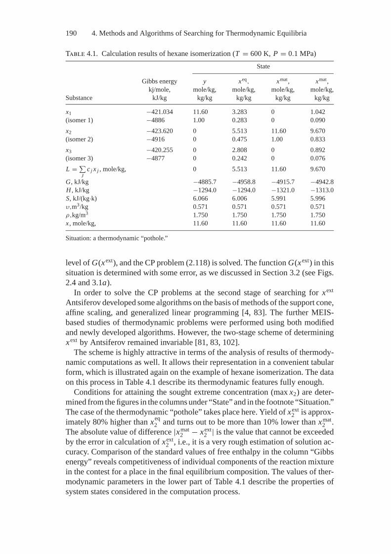
190 4. Methods and Algorithms of Searching for Thermodynamic Equilibria
Table 4.1. Calculation results of hexane isomerization (T = 600 K, P = 0.1 MPa)
State
Gibbs energy y xeq, xmat, xmat,kj/mole, mole/kg, mole/kg, mole/kg, mole/kg,
Substance kJ/kg kg/kg kg/kg kg/kg kg/kg
x1 −421.034 11.60 3.283 0 1.042(isomer 1) −4886 1.00 0.283 0 0.090x2 −423.620 0 5.513 11.60 9.670(isomer 2) −4916 0 0.475 1.00 0.833x3 −420.255 0 2.808 0 0.892(isomer 3) −4877 0 0.242 0 0.076L = ∑
Jc j x j , mole/kg, 0 5.513 11.60 9.670
G, kJ/kg −4885.7 −4958.8 −4915.7 −4942.8H , kJ/kg −1294.0 −1294.0 −1321.0 −1313.0S, kJ/(kg·k) 6.066 6.006 5.991 5.996υ,m3/kg 0.571 0.571 0.571 0.571ρ,kg/m3 1.750 1.750 1.750 1.750x , mole/kg, 11.60 11.60 11.60 11.60
Situation: a thermodynamic “pothole.”
level of G(xext), and the CP problem (2.118) is solved. The function G(xext) in thissituation is determined with some error, as we discussed in Section 3.2 (see Figs.2.4 and 3.1a).
In order to solve the CP problems at the second stage of searching for xext
Antsiferov developed some algorithms on the basis of methods of the support cone,affine scaling, and generalized linear programming [4, 83]. The further MEIS-based studies of thermodynamic problems were performed using both modifiedand newly developed algorithms. However, the two-stage scheme of determiningxext by Antsiferov remained invariable [81, 83, 102].
The scheme is highly attractive in terms of the analysis of results of thermody-namic computations as well. It allows their representation in a convenient tabularform, which is illustrated again on the example of hexane isomerization. The dataon this process in Table 4.1 describe its thermodynamic features fully enough.
Conditions for attaining the sought extreme concentration (max x2) are deter-mined from the figures in the columns under “State” and in the footnote “Situation.”The case of the thermodynamic “pothole” takes place here. Yield of xext
2 is approx-imately 80% higher than xeq
2 and turns out to be more than 10% lower than xmat2 .
The absolute value of difference |xmat2 − xext
2 | is the value that cannot be exceededby the error in calculation of xext
2 , i.e., it is a very rough estimation of solution ac-curacy. Comparison of the standard values of free enthalpy in the column “Gibbsenergy” reveals competitiveness of individual components of the reaction mixturein the contest for a place in the final equilibrium composition. The values of ther-modynamic parameters in the lower part of Table 4.1 describe the properties ofsystem states considered in the computation process.
4.2. Optimization of the Initial Composition of Reagents 191
Numerous calculations of most diverse systems (technical and natural) demon-strated high efficiency of the algorithm of stage 1 of Antsiferov’s scheme. Theresults were always logically consistent. In rare cases, when it was possible toestimate calculation accuracy more correctly than to find them by comparison be-tween values of xext and xmat, the estimates were acceptable. This does not mean,however, that in the future one will not run across such situations where the er-rors in determining G(xext) will be impermissibly large. Therefore, the problemof devising alternative methods of searching for xext is topical. Construction ofalgorithms on the basis of the idea of a thermodynamic tree seems to be a possiblealternative to Antsiferov’s scheme.
The next Sections of this chapter dwell on algorithms for determination of yext
and xext (stage 2 of calculations made using Antsiferov’s technique) and the alterna-tive algorithm for determination of G(xext) based on the idea of the thermodynamictree (stage 1 of calculations made using Antsiferov’s technique). The last section,Section 4.5, presents preliminary considerations on the technique for estimatingfeasibility and stability of the partial equilibria of xext.
4.2. Optimization of the Initial Composition of Reagentsin a Chemical System by the Simplex Embedding Method
It is difficult to apply MEIS (2.43)–(2.50) of systems with a variable initial com-position of reagents for choosing an optimal value of y because, in the problemstatement, the vectors x andy are analytically independent. Therefore, it is com-plicated to apply methods requiring that functions and their derivatives—ones thatdepend simultaneously on the values of these two vectors—be calculated in theiterative process.
To solve a general problem of searching for the point (xext, yext) E.G. Antsiferovapplied the simplex embedding method to determine yext [6].
The simplex belonging to the Euclidean space Rn with the vertex at the pointx0 and the edges x1 − x0, . . . , xn − x0, that form the basis in Rn is a polyhedron,all points of which satisfy the condition
x = x0 +n∑
i=1αi (xi − x0) ,
n∑i=1
αi ≤ 1, αi ≥ 0. (4.1)
Without loss of generality it is assumed that x0 = 0, i.e., x0 coincides with thecoordinate origin. The simplex volume is determined by the formula
V = [det (x)]n , (4.2)
where x is an n × n matrix whose rows are the transposed vectors of coordinatesof the vertices. The simplex center is found from the expression
xc = (x0 + · · · + xn)(n + 1)
. (4.3)
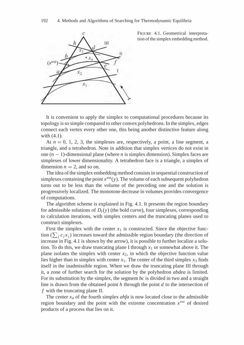
192 4. Methods and Algorithms of Searching for Thermodynamic Equilibria
(xext)
Figure 4.1. Geometrical interpreta-tion of the simplex embedding method.
It is convenient to apply the simplex to computational procedures because itstopology is so simple compared to other convex polyhedrons. In the simplex, edgesconnect each vertex every other one, this being another distinctive feature alongwith (4.1).
At n = 0, 1, 2, 3, the simplexes are, respectively, a point, a line segment, atriangle, and a tetrahedron. Note in addition that simplex vertices do not exist inone (n − 1)-dimensional plane (where n is simplex dimension). Simplex faces aresimplexes of lower dimensionality. A tetrahedron face is a triangle, a simplex ofdimension n = 2, and so on.
The idea of the simplex embedding method consists in sequential construction ofsimplexes containing the point xext(y). The volume of each subsequent polyhedronturns out to be less than the volume of the preceding one and the solution isprogressively localized. The monotone decrease in volumes provides convergenceof computations.
The algorithm scheme is explained in Fig. 4.1. It presents the region boundaryfor admissible solutions of Dt (y) (the bold curve), four simplexes, correspondingto calculation iterations, with simplex centers and the truncating planes used toconstruct simplexes.
First the simplex with the center x1 is constructed. Since the objective func-tion (
∑j c j x j ) increases toward the admissible region boundary (the direction of
increase in Fig. 4.1 is shown by the arrow), it is possible to further localize a solu-tion. To do this, we draw truncating plane I through x1 or somewhat above it. Theplane isolates the simplex with center x2, in which the objective function valuelies higher than in simplex with center x1. The center of the third simplex x3 findsitself in the inadmissible region. When we draw the truncating plane III throughit, a zone of further search for the solution by the polyhedron abdea is limited.For its substitution by the simplex, the segment bc is divided in two and a straightline is drawn from the obtained point h through the point d to the intersection off with the truncating plane II.
The center x4 of the fourth simplex ahfa is now located close to the admissibleregion boundary and the point with the extreme concentration xext of desiredproducts of a process that lies on it.
4.2. Optimization of the Initial Composition of Reagents 193
As is seen from equation (4.1), the simplex embedding method requires that theproblem constraints be set as non-homogeneous inequalities. Conditions (2.47),which determine admissible relations among the yvector components, can appar-ently be rewritten in the form
l∑j=1
αk j y j ≤ 0, k ∈ K . (4.4)
To pass from (4.4) to nonhomogeneous inequalities, some variable, the first, forexample, will be expressed through the remaining ones based on the normalizationcondition (2.44):
y1 = 1 −
l∑j=2
M j y j
M1. (4.5)
Then the initial simplex is determined by the obvious inequalityl∑
j=2
M j
M1y j ≤ 1, (4.6)
where all M jM1
are strictly greater than zero.The truncating plane is constructed using the solution (x) of the following CP
problem:Find
maxn∑
j=1c j x j (4.7)
subject to
Ax = b (yc) =n∑
j=1y j A j , (4.8)
G (x) = G (yc) , (4.9)x j > 0, (4.10)
where yc and G(yc) are the simplex center and the associated Gibbs energy level,respectively, and A j is the j th column of the matrix A. The solution x along with(4.8)–(4.10) satisfies the Kuhn–Tucker conditions:
c j =m∑
i=1λi ai j + λm+1∇ j G (x) , (4.11)
λm+1 > 0, (4.12)
where ∇ j G(x) is the j th component of the gradient G(x) at the point x .Let us increase the initial component yc by a small value �y. This will involve
a change in the material balances (4.8), and the relation (4.9):
G (x) ≤ G (yc) .
194 4. Methods and Algorithms of Searching for Thermodynamic Equilibria
The optimal solution x and the objective function (4.7) will also change. Theformer will increase by �x and the latter by c�x . If �y is chosen to be rathersmall, the set of active constraints and the dual solution to problem (4.7)–(4.10)will remain invariable.
In a linear approximation variation of the solution, �x will satisfy the conditions:
A�x =l∑
j=1�y j A j , (4.13)
∇T G (x) �x = ∇T G (yc) �y. (4.14)
If we multiply equality (4.13) by λi , i = 1, . . . , m, equality (4.14) by λm+1, addthe results, and take into consideration (4.11), the objective function (4.7) will be
�F =l∑
j=1
[m∑
i=1λi ai j + λm+1∇G (yc)
]�y j . (4.15)
Based on (4.11) the formula for the truncating half-space in the y variables canbe written:
dT (y − yc) ≥ 0, (4.16)
where
d j = a j
� (yc)−
(cT x
)� (yc)2 , (4.17)
a j =m∑
i=1λi ai j + λm+1∇G (yc) , (4.18)
� (yc) =∑j∈Jc
y j . (4.19)
This algorithm can check admissibility of a simplex center at each iteration interms of yield of substances of interest to the researcher.
4.3. Calculations of Complete and Partial Equilibriaby the Affine Scaling Method
The point of the final equilibrium xeq on the material balance polyhedron D(y) issometimes sought by the Lagrange multipliers method (see, for example, [9]. Thesystem of equations obtained in this case by equating the partial derivatives of Lto zero is solved by the Newton method or some other method. Such an approachis suitable when xeq is an interior point of D(y). However, in Chapter 2 it wasshown that this condition is not fulfilled when the thermodynamic system containscondensed phases. Besides, the method of multipliers is difficult to apply wheninequality constraints are included in the models of final equilibria.
4.3. Calculations of Complete and Partial Equilibria 195
Applicability of the multipliers method to calculate xext (model (2.38)–(2.42))becomes even more problematic than searching for xeq because of the necessityto consider a wide diversity of constraints. Therefore, we applied solely the MPmethods for searching for xeq and xext 1. Here we will dwell on the affine scal-ing method that has been used most often so far in studies on thermodynamicattainability regions and partial equilibria [34, 35].
The affine scaling method is convenient because it handles only the interiorpoints of D(y), in which an objective function gradient can be calculated andthe motion to the extremum point is executed at an acute angle to this gradienttaken with the opposite sign. The latter circumstance facilitates convergence ofthe method at an unfavorable (with the zones of small steepness) surface shape,on which the extremum point is sought. Using the figurative comparison we willexplain that when descending the mountain by this method we determine mo-tion direction not by touch, as in the steepest descent method, but by choos-ing the lowest point in the visible vicinity and adjusting the route after reachingit.
The idea of the above method will be illustrated with the example of searching forthe point xeq. An initial point for the computational process is some interior pointx0 of the polyhedron D(y), at which x0
j > 0 for all j = 1, . . . , n. At each iterationk = 0, 1, 2, . . ., the obvious conditions on conservation of the mole quantities ofelements and their positiveness are assumed:
n∑j=1
ai j(x j − xk
j) = 0, xk
j > 0. (4.20)
The correction vector = ( k1, . . . ,
kn)T whose components are (x j − xk
j )determines direction of the motion at the kth iteration.
The ellipsoid is constructed with center at xk such thatn∑
j=1
2j
(xkj )2
≤ 1, (4.21)
which represents a “visible vicinity.” This means the ellipsoid axes are distancesfrom xk to the positive orthant boundaries that determine a “visibility zone” subjectto (4.20).
The point with the minimum Gibbs energy is sought by the lineariza-tion technique, i.e., the partial derivatives of the function G(x) are calculatedas
gkj = ∂G
(xk)
∂x j, (4.22)
1 Indicating the problems in application of the multipliers method, we mean its applicationas the basic procedure of computational algorithms. As an auxiliary procedure this methodis included in many MP algorithms.
196 4. Methods and Algorithms of Searching for Thermodynamic Equilibria
and the minimum value of the linear form is determined to be
C =n∑
j=1gk
j j (4.23)
subject ton∑
j=1ai j j = 0, (4.24)
n∑j=1
2j(
xkj
)2 = 1. (4.25)
As compared to (4.21) the strict equality sign is used in (4.25), since the linearfunction reaches its minimum at the boundary point of the convex set, in this caseon the ellipsoid surface or the plane of its intersection with the material balancepolyhedron.
The solution of problem (4.23)–(4.25) is found using the system of equationsobtained as a result of equating partial derivatives of the Lagrange functions (4.26)to zero:
L ( , λ) =n∑
j=1gk
j j −m∑
i=1λi
n∑j=1
ai j j + λm+1
⎛⎜⎝1 −
n∑j=1
2j(
xkj
)2
⎞⎟⎠ . (4.26)
The solution thus is represented by the formulas
j = (xk
j)2
m∑i=1
λ i ai j − gkj
2λm+1, (4.27)
2λm+1 =⎛⎝ n∑
j=1
(xk
j)2
(m∑
i=1λi ai j − gk
j
)2⎞⎠
0.5
, (4.28)
λ = g A−1, (4.29)
where λ is a vector of the Lagrange multipliers with material balance constraintsthat include m components of λi . The iteration k terminates when the interiorpoint xk+1 is determined, at which the minimum of function G(x) is reached onthe segment that coincides with its direction and is equal to the absolute value of .
The process is repeated, until the magnitude
Fk = 4λ2m+1 =
n∑j=1
(xk
j)2
(m∑
i=1λi ai j − gk
j
)2
(4.30)
becomes less than the given small number ε. The sense of a rule that interruptsthe process is clear, since the negligibly low value of Fk is associated with the
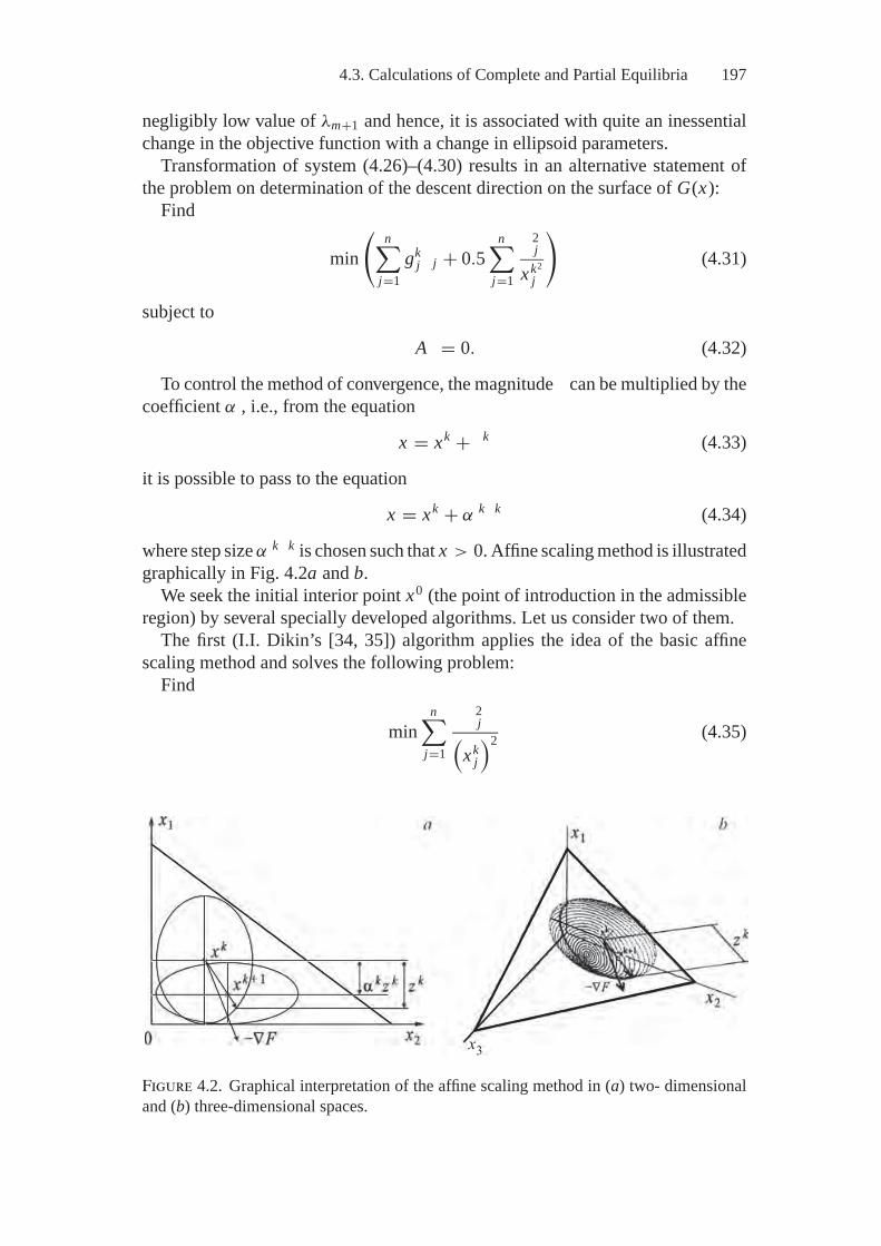
4.3. Calculations of Complete and Partial Equilibria 197
negligibly low value of λm+1 and hence, it is associated with quite an inessentialchange in the objective function with a change in ellipsoid parameters.
Transformation of system (4.26)–(4.30) results in an alternative statement ofthe problem on determination of the descent direction on the surface of G(x):
Find
min
(n∑
j=1gk
j j + 0.5n∑
j=1
2j
xk2
j
)(4.31)
subject to
A = 0. (4.32)
To control the method of convergence, the magnitude can be multiplied by thecoefficient α , i.e., from the equation
x = xk + k (4.33)
it is possible to pass to the equation
x = xk + α k k (4.34)
where step size α k k is chosen such that x > 0. Affine scaling method is illustratedgraphically in Fig. 4.2a and b.
We seek the initial interior point x0 (the point of introduction in the admissibleregion) by several specially developed algorithms. Let us consider two of them.
The first (I.I. Dikin’s [34, 35]) algorithm applies the idea of the basic affinescaling method and solves the following problem:
Find
minn∑
j=1
2j(
xkj
)2 (4.35)
Figure 4.2. Graphical interpretation of the affine scaling method in (a) two- dimensionaland (b) three-dimensional spaces.
198 4. Methods and Algorithms of Searching for Thermodynamic Equilibria
subject to
A = rk, (4.36)
where
rk = b − Axk . (4.37)
Transition from xk to xk+1 is performed by equation (4.34), αk is taken such thatxk+1 belongs to the interior admissible region. The step size should not exceedunity, in this case. The calculation terminates when the absolute value of theimbalance |rk | becomes less than the given value ε .
Search for x0 by the second (E.G. Antsiferov’s) algorithm is based on the solutionto the following auxiliary LP problem:
Findmax �
subject ton∑
j=1ai j y j + �
n∑j=1
ai j = bi i = 1, . . . , m, y j ≥ 0, � > 0
⎫⎪⎪⎪⎪⎪⎬⎪⎪⎪⎪⎪⎭
(4.38)
Components of the vector x0 are determined by the formula x0j = y j + � . The
second algorithm is apparently easier to apply then the first.The solution of x0 found by any of the mentioned algorithms can be additionally
corrected based on the fact that all the interior points of the segment [x0, y] are theinterior points of D(y). For example, it seems logical to choose a minimum Gibbsenergy point on this intercept as an initial approximation in the search for xeq. Thechoice may contribute to an increase in the convergence rate of computations.
When the affine scaling method is used for searching for the point xext, theformulas to calculate the coefficients g j in the objective function (4.23) change,and additional members on the right-hand side of equation (4.26) appear that cor-respond to constraints on the Gibbs energy values in the models of type (2.116) or(2.118). The general scheme of algorithm application, however, remains invariable.
Despite the fact that the affine scaling method proved to be highly efficientfor solving a large number of applied thermodynamic problems, there are casesof extremely slow convergence such as in the solution of environmental prob-lems, where the spread in values of the sought variables reaches 10–12 orders ofmagnitude and higher.
This problem was solved by I.A. Shirkalin [156]. He revealed a sharp deceler-ation of convergence of the discussed method near the point xeq when concentra-tions of part of the reaction mixture components approach zero. In the search for adirection of optimal descent ( ) he formulated the simplest two-dimensional prob-lem, introducing three assumptions: 1) the initial point x0 is close to the solution;2) the objective function is strictly convex and twice continuously differentiable;3) the value of the second coordinate (r ) is much lower than that of the first (R).
Shirkalin determined the coordinates by expansion of the objective functioninto the Taylor power series, = x − x0, and employed just the first three members
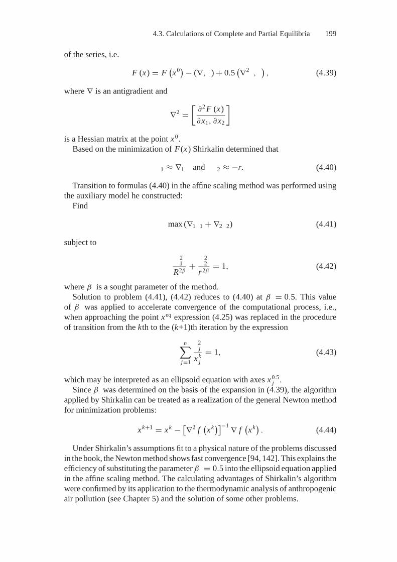
4.3. Calculations of Complete and Partial Equilibria 199
of the series, i.e.
F (x) = F(x0) − (∇, ) + 0.5
(∇2 ,), (4.39)
where ∇ is an antigradient and
∇2 =[
∂2 F (x)∂x1, ∂x2
]
is a Hessian matrix at the point x0.Based on the minimization of F(x) Shirkalin determined that
1 ≈ ∇1 and 2 ≈ −r. (4.40)
Transition to formulas (4.40) in the affine scaling method was performed usingthe auxiliary model he constructed:
Find
max (∇1 1 + ∇2 2) (4.41)
subject to
21
R2β+
22
r2β= 1, (4.42)
where β is a sought parameter of the method.Solution to problem (4.41), (4.42) reduces to (4.40) at β = 0.5. This value
of β was applied to accelerate convergence of the computational process, i.e.,when approaching the point xeq expression (4.25) was replaced in the procedureof transition from the kth to the (k+1)th iteration by the expression
n∑j=1
2j
xkj
= 1, (4.43)
which may be interpreted as an ellipsoid equation with axes x0.5j .
Since β was determined on the basis of the expansion in (4.39), the algorithmapplied by Shirkalin can be treated as a realization of the general Newton methodfor minimization problems:
xk+1 = xk − [∇2 f(xk)]−1 ∇ f
(xk) . (4.44)
Under Shirkalin’s assumptions fit to a physical nature of the problems discussedin the book, the Newton method shows fast convergence [94, 142]. This explains theefficiency of substituting the parameter β = 0.5 into the ellipsoid equation appliedin the affine scaling method. The calculating advantages of Shirkalin’s algorithmwere confirmed by its application to the thermodynamic analysis of anthropogenicair pollution (see Chapter 5) and the solution of some other problems.
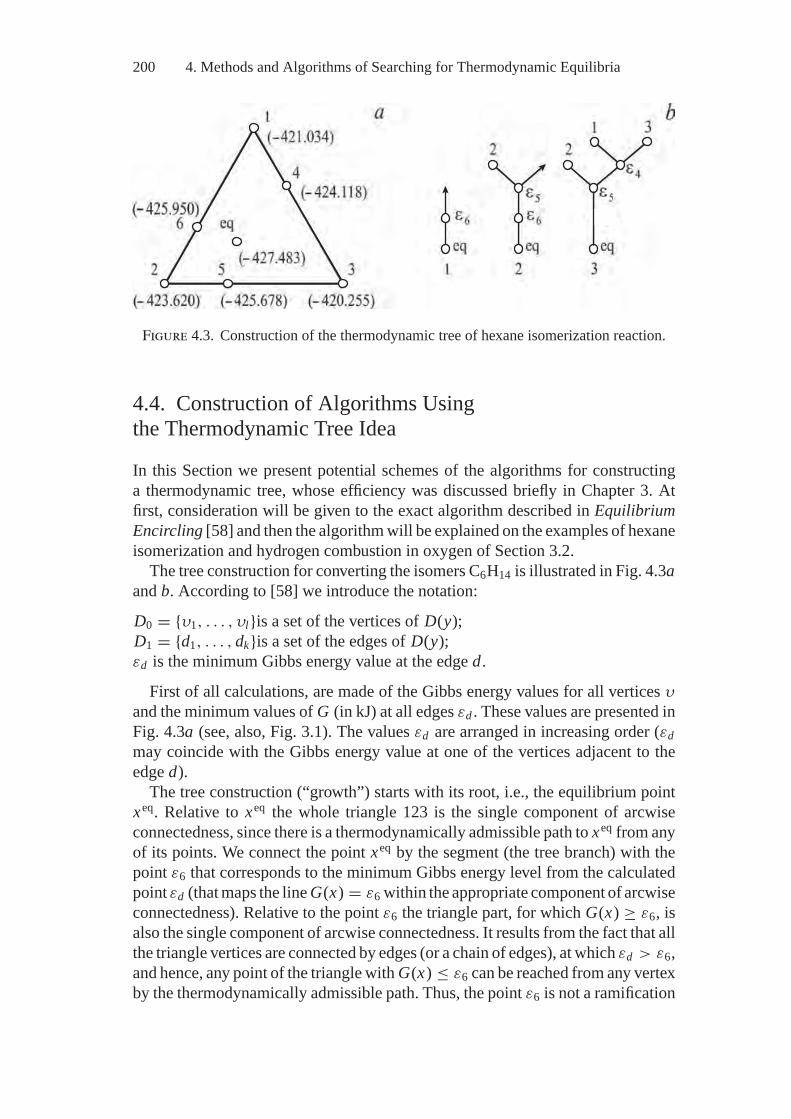
200 4. Methods and Algorithms of Searching for Thermodynamic Equilibria
Figure 4.3. Construction of the thermodynamic tree of hexane isomerization reaction.
4.4. Construction of Algorithms Usingthe Thermodynamic Tree Idea
In this Section we present potential schemes of the algorithms for constructinga thermodynamic tree, whose efficiency was discussed briefly in Chapter 3. Atfirst, consideration will be given to the exact algorithm described in EquilibriumEncircling [58] and then the algorithm will be explained on the examples of hexaneisomerization and hydrogen combustion in oxygen of Section 3.2.
The tree construction for converting the isomers C6H14 is illustrated in Fig. 4.3aand b. According to [58] we introduce the notation:
D0 = {υ1, . . . , υl}is a set of the vertices of D(y);D1 = {d1, . . . , dk}is a set of the edges of D(y);εd is the minimum Gibbs energy value at the edge d.
First of all calculations, are made of the Gibbs energy values for all vertices υ
and the minimum values of G (in kJ) at all edges εd . These values are presented inFig. 4.3a (see, also, Fig. 3.1). The values εd are arranged in increasing order (εdmay coincide with the Gibbs energy value at one of the vertices adjacent to theedge d).
The tree construction (“growth”) starts with its root, i.e., the equilibrium pointxeq. Relative to xeq the whole triangle 123 is the single component of arcwiseconnectedness, since there is a thermodynamically admissible path to xeq from anyof its points. We connect the point xeq by the segment (the tree branch) with thepoint ε6 that corresponds to the minimum Gibbs energy level from the calculatedpoint εd (that maps the line G(x) = ε6 within the appropriate component of arcwiseconnectedness). Relative to the point ε6 the triangle part, for which G(x) ≥ ε6, isalso the single component of arcwise connectedness. It results from the fact that allthe triangle vertices are connected by edges (or a chain of edges), at which εd > ε6,and hence, any point of the triangle with G(x) ≤ ε6 can be reached from any vertexby the thermodynamically admissible path. Thus, the point ε6 is not a ramification
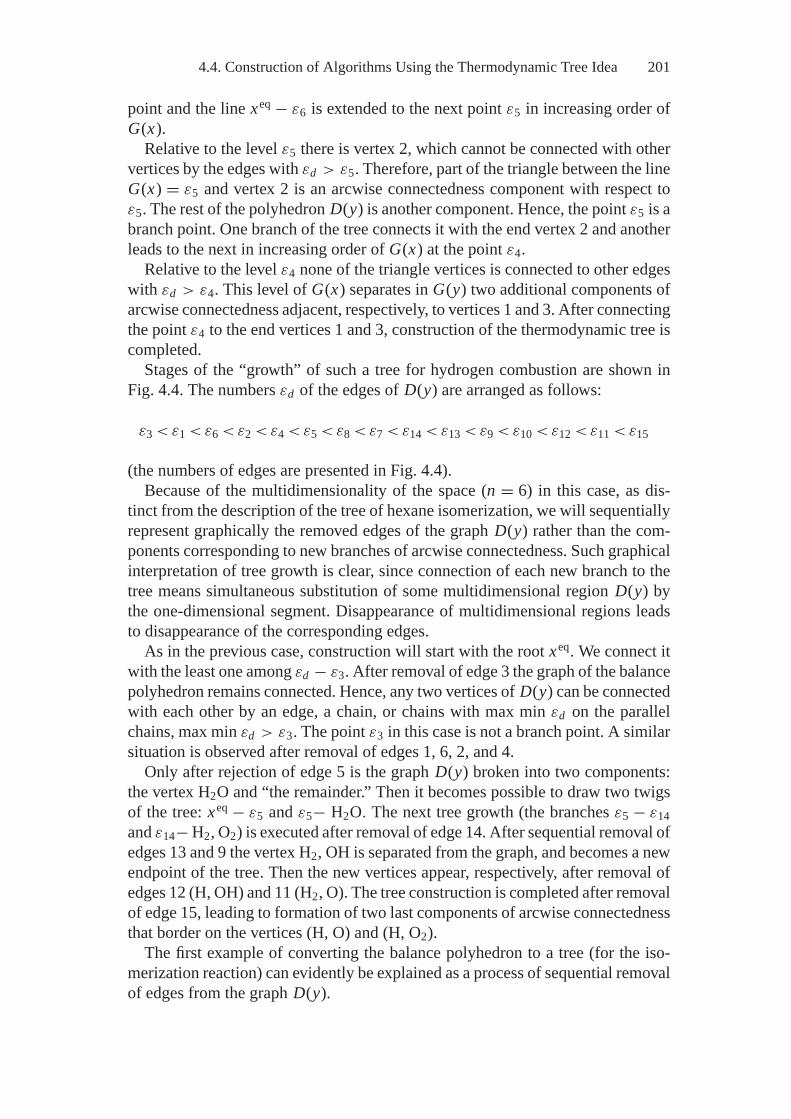
4.4. Construction of Algorithms Using the Thermodynamic Tree Idea 201
point and the line xeq − ε6 is extended to the next point ε5 in increasing order ofG(x).
Relative to the level ε5 there is vertex 2, which cannot be connected with othervertices by the edges with εd > ε5. Therefore, part of the triangle between the lineG(x) = ε5 and vertex 2 is an arcwise connectedness component with respect toε5. The rest of the polyhedron D(y) is another component. Hence, the point ε5 is abranch point. One branch of the tree connects it with the end vertex 2 and anotherleads to the next in increasing order of G(x) at the point ε4.
Relative to the level ε4 none of the triangle vertices is connected to other edgeswith εd > ε4. This level of G(x) separates in G(y) two additional components ofarcwise connectedness adjacent, respectively, to vertices 1 and 3. After connectingthe point ε4 to the end vertices 1 and 3, construction of the thermodynamic tree iscompleted.
Stages of the “growth” of such a tree for hydrogen combustion are shown inFig. 4.4. The numbers εd of the edges of D(y) are arranged as follows:
ε3 < ε1 < ε6 < ε2 < ε4 < ε5 < ε8 < ε7 < ε14 < ε13 < ε9 < ε10 < ε12 < ε11 < ε15
(the numbers of edges are presented in Fig. 4.4).Because of the multidimensionality of the space (n = 6) in this case, as dis-
tinct from the description of the tree of hexane isomerization, we will sequentiallyrepresent graphically the removed edges of the graph D(y) rather than the com-ponents corresponding to new branches of arcwise connectedness. Such graphicalinterpretation of tree growth is clear, since connection of each new branch to thetree means simultaneous substitution of some multidimensional region D(y) bythe one-dimensional segment. Disappearance of multidimensional regions leadsto disappearance of the corresponding edges.
As in the previous case, construction will start with the root xeq. We connect itwith the least one among εd − ε3. After removal of edge 3 the graph of the balancepolyhedron remains connected. Hence, any two vertices of D(y) can be connectedwith each other by an edge, a chain, or chains with max min εd on the parallelchains, max min εd > ε3. The point ε3 in this case is not a branch point. A similarsituation is observed after removal of edges 1, 6, 2, and 4.
Only after rejection of edge 5 is the graph D(y) broken into two components:the vertex H2O and “the remainder.” Then it becomes possible to draw two twigsof the tree: xeq − ε5 and ε5− H2O. The next tree growth (the branches ε5 − ε14and ε14− H2, O2) is executed after removal of edge 14. After sequential removal ofedges 13 and 9 the vertex H2, OH is separated from the graph, and becomes a newendpoint of the tree. Then the new vertices appear, respectively, after removal ofedges 12 (H, OH) and 11 (H2, O). The tree construction is completed after removalof edge 15, leading to formation of two last components of arcwise connectednessthat border on the vertices (H, O) and (H, O2).
The first example of converting the balance polyhedron to a tree (for the iso-merization reaction) can evidently be explained as a process of sequential removalof edges from the graph D(y).
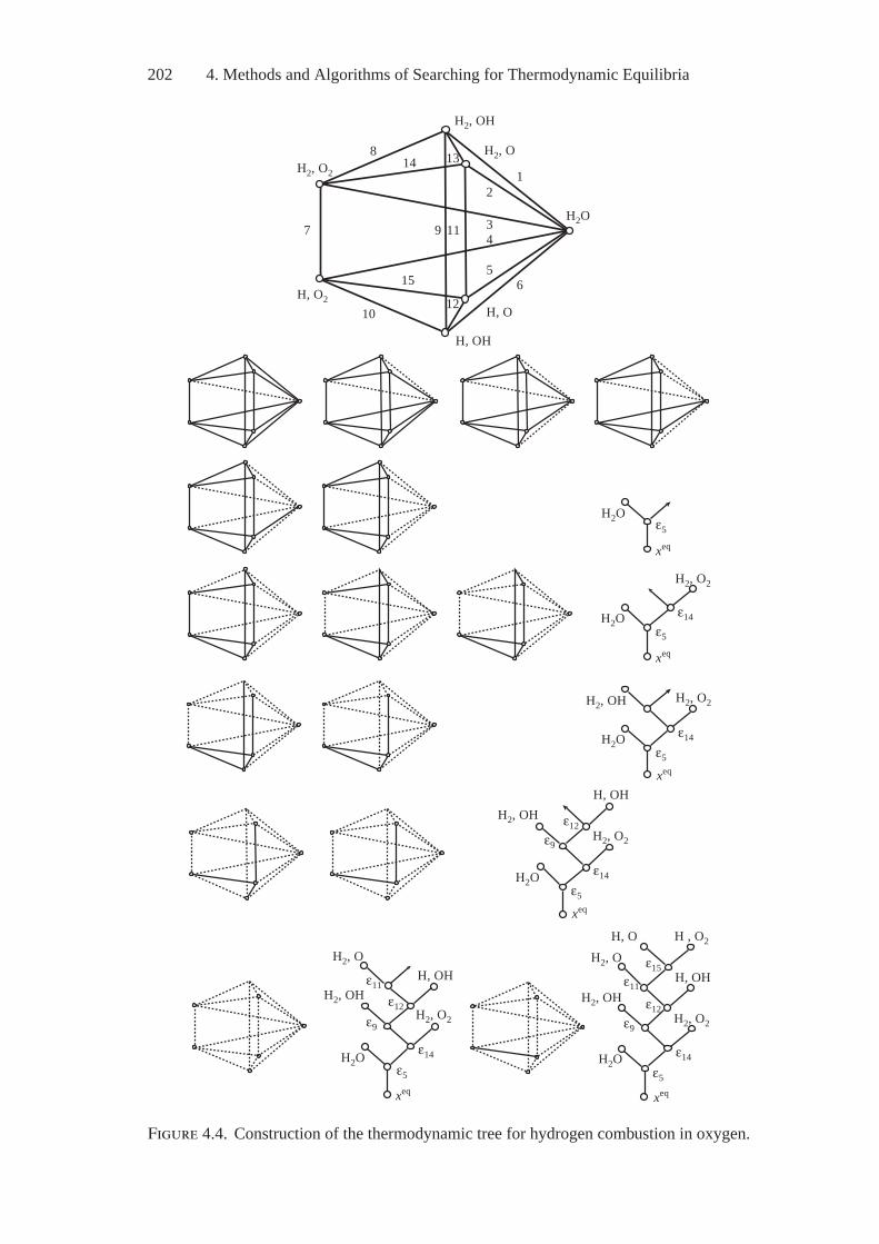
202 4. Methods and Algorithms of Searching for Thermodynamic Equilibria
H2, OH
H, OH
H, OH
H, O
H, OHH, OH
H, O
7 9 11
12
15
10H, O2
H2, O
H2O
H2O
H2, O2
H2, O2
H2, O2H2, O2
H2, OH2, OH , O2
H2, O2
H2, OH
H2, OH
H2, OHH2, OH
H2O
H2O
H2OH2O
H2O
ε5
ε5
ε5
ε14
ε12
ε9
ε14
xeq
xeq
xeq
ε5
ε5ε5
ε14
ε14ε14
xeq
xeqxeq
ε11ε11
ε12ε12
ε15
ε9ε9
H2, O2
814 13
12
34
56
Figure 4.4. Construction of the thermodynamic tree for hydrogen combustion in oxygen.
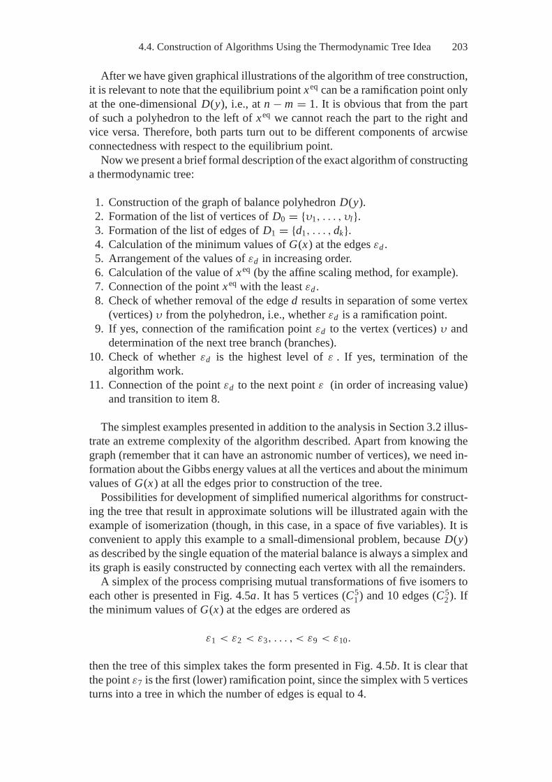
4.4. Construction of Algorithms Using the Thermodynamic Tree Idea 203
After we have given graphical illustrations of the algorithm of tree construction,it is relevant to note that the equilibrium point xeq can be a ramification point onlyat the one-dimensional D(y), i.e., at n − m = 1. It is obvious that from the partof such a polyhedron to the left of xeq we cannot reach the part to the right andvice versa. Therefore, both parts turn out to be different components of arcwiseconnectedness with respect to the equilibrium point.
Now we present a brief formal description of the exact algorithm of constructinga thermodynamic tree:
1. Construction of the graph of balance polyhedron D(y).2. Formation of the list of vertices of D0 = {υ1, . . . , υl}.3. Formation of the list of edges of D1 = {d1, . . . , dk}.4. Calculation of the minimum values of G(x) at the edges εd .5. Arrangement of the values of εd in increasing order.6. Calculation of the value of xeq (by the affine scaling method, for example).7. Connection of the point xeq with the least εd .8. Check of whether removal of the edge d results in separation of some vertex
(vertices) υ from the polyhedron, i.e., whether εd is a ramification point.9. If yes, connection of the ramification point εd to the vertex (vertices) υ and
determination of the next tree branch (branches).10. Check of whether εd is the highest level of ε . If yes, termination of the
algorithm work.11. Connection of the point εd to the next point ε (in order of increasing value)
and transition to item 8.
The simplest examples presented in addition to the analysis in Section 3.2 illus-trate an extreme complexity of the algorithm described. Apart from knowing thegraph (remember that it can have an astronomic number of vertices), we need in-formation about the Gibbs energy values at all the vertices and about the minimumvalues of G(x) at all the edges prior to construction of the tree.
Possibilities for development of simplified numerical algorithms for construct-ing the tree that result in approximate solutions will be illustrated again with theexample of isomerization (though, in this case, in a space of five variables). It isconvenient to apply this example to a small-dimensional problem, because D(y)as described by the single equation of the material balance is always a simplex andits graph is easily constructed by connecting each vertex with all the remainders.
A simplex of the process comprising mutual transformations of five isomers toeach other is presented in Fig. 4.5a. It has 5 vertices (C5
1 ) and 10 edges (C52 ). If
the minimum values of G(x) at the edges are ordered as
ε1 < ε2 < ε3, . . . , < ε9 < ε10.
then the tree of this simplex takes the form presented in Fig. 4.5b. It is clear thatthe point ε7 is the first (lower) ramification point, since the simplex with 5 verticesturns into a tree in which the number of edges is equal to 4.
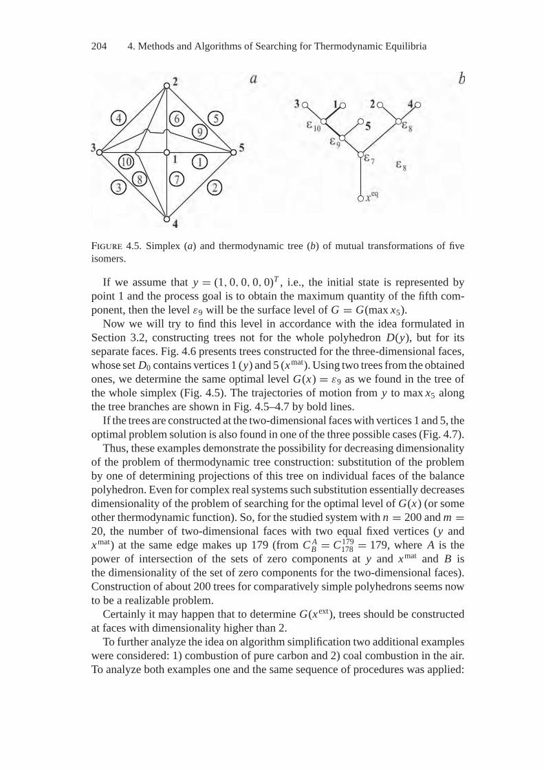
204 4. Methods and Algorithms of Searching for Thermodynamic Equilibria
Figure 4.5. Simplex (a) and thermodynamic tree (b) of mutual transformations of fiveisomers.
If we assume that y = (1, 0, 0, 0, 0)T , i.e., the initial state is represented bypoint 1 and the process goal is to obtain the maximum quantity of the fifth com-ponent, then the level ε9 will be the surface level of G = G(max x5).
Now we will try to find this level in accordance with the idea formulated inSection 3.2, constructing trees not for the whole polyhedron D(y), but for itsseparate faces. Fig. 4.6 presents trees constructed for the three-dimensional faces,whose set D0 contains vertices 1 (y) and 5 (xmat). Using two trees from the obtainedones, we determine the same optimal level G(x) = ε9 as we found in the tree ofthe whole simplex (Fig. 4.5). The trajectories of motion from y to max x5 alongthe tree branches are shown in Fig. 4.5–4.7 by bold lines.
If the trees are constructed at the two-dimensional faces with vertices 1 and 5, theoptimal problem solution is also found in one of the three possible cases (Fig. 4.7).
Thus, these examples demonstrate the possibility for decreasing dimensionalityof the problem of thermodynamic tree construction: substitution of the problemby one of determining projections of this tree on individual faces of the balancepolyhedron. Even for complex real systems such substitution essentially decreasesdimensionality of the problem of searching for the optimal level of G(x) (or someother thermodynamic function). So, for the studied system with n = 200 and m =20, the number of two-dimensional faces with two equal fixed vertices (y andxmat) at the same edge makes up 179 (from C A
B = C179178 = 179, where A is the
power of intersection of the sets of zero components at y and xmat and B isthe dimensionality of the set of zero components for the two-dimensional faces).Construction of about 200 trees for comparatively simple polyhedrons seems nowto be a realizable problem.
Certainly it may happen that to determine G(xext), trees should be constructedat faces with dimensionality higher than 2.
To further analyze the idea on algorithm simplification two additional exampleswere considered: 1) combustion of pure carbon and 2) coal combustion in the air.To analyze both examples one and the same sequence of procedures was applied:
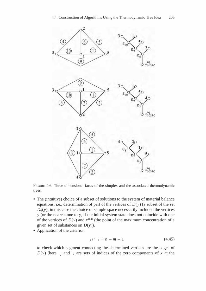
4.4. Construction of Algorithms Using the Thermodynamic Tree Idea 205
1
Figure 4.6. Three-dimensional faces of the simplex and the associated thermodynamictrees.
� The (intuitive) choice of a subset of solutions to the system of material balanceequations, i.e., determination of part of the vertices of D(y) (a subset of the setD0(y); in this case the choice of sample space necessarily included the verticesy (or the nearest one to y, if the initial system state does not coincide with oneof the vertices of D(y) and xmat (the point of the maximum concentration of agiven set of substances on D(y)).
� Application of the criterion
j ∩ i = n − m − 1 (4.45)
to check which segment connecting the determined vertices are the edges ofD(y) (here j and i are sets of indices of the zero components of x at the
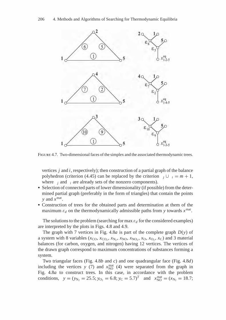
206 4. Methods and Algorithms of Searching for Thermodynamic Equilibria
Figure 4.7. Two-dimensional faces of the simplex and the associated thermodynamic trees.
vertices j and i , respectively); then construction of a partial graph of the balancepolyhedron (criterion (4.45) can be replaced by the criterion j ∪ i = m + 1,where j and i are already sets of the nonzero components).
� Selection of connected parts of lower dimensionality (if possible) from the deter-mined partial graph (preferably in the form of triangles) that contain the pointsy and xmat.
� Construction of trees for the obtained parts and determination at them of themaximum εd on the thermodynamically admissible paths from y towards xmat.
The solutions to the problem (searching for max εd for the considered examples)are interpreted by the plots in Figs. 4.8 and 4.9.
The graph with 7 vertices in Fig. 4.8a is part of the complete graph D(y) ofa system with 8 variables (xCO, xCO2 , xN2 , xNO, xNO2 , xO, xO2 , xC) and 3 materialbalances (for carbon, oxygen, and nitrogen) having 12 vertices. The vertices ofthe drawn graph correspond to maximum concentrations of substances forming asystem.
Two triangular faces (Fig. 4.8b and c) and one quadrangular face (Fig. 4.8d)including the vertices y (7) and xmat
NO (4) were separated from the graph inFig. 4.8a to construct trees. In this case, in accordance with the problemconditions, y = (yN2 = 25.5; yO2 = 6.8; yC = 5.7)T and xmat
NO = (xN2 = 18.7;
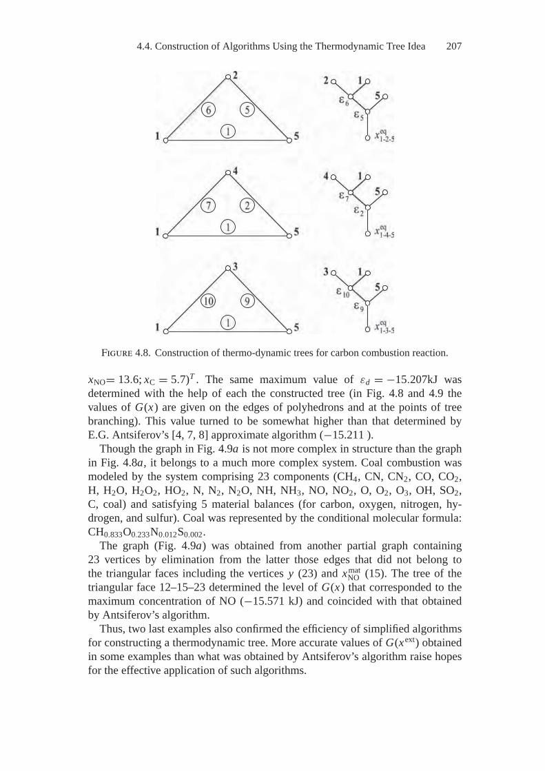
4.4. Construction of Algorithms Using the Thermodynamic Tree Idea 207
Figure 4.8. Construction of thermo-dynamic trees for carbon combustion reaction.
xNO= 13.6; xC = 5.7)T . The same maximum value of εd = −15.207kJ wasdetermined with the help of each the constructed tree (in Fig. 4.8 and 4.9 thevalues of G(x) are given on the edges of polyhedrons and at the points of treebranching). This value turned to be somewhat higher than that determined byE.G. Antsiferov’s [4, 7, 8] approximate algorithm (−15.211 ).
Though the graph in Fig. 4.9a is not more complex in structure than the graphin Fig. 4.8a, it belongs to a much more complex system. Coal combustion wasmodeled by the system comprising 23 components (CH4, CN, CN2, CO, CO2,H, H2O, H2O2, HO2, N, N2, N2O, NH, NH3, NO, NO2, O, O2, O3, OH, SO2,C, coal) and satisfying 5 material balances (for carbon, oxygen, nitrogen, hy-drogen, and sulfur). Coal was represented by the conditional molecular formula:CH0.833O0.233N0.012S0.002.
The graph (Fig. 4.9a) was obtained from another partial graph containing23 vertices by elimination from the latter those edges that did not belong tothe triangular faces including the vertices y (23) and xmat
NO (15). The tree of thetriangular face 12–15–23 determined the level of G(x) that corresponded to themaximum concentration of NO (−15.571 kJ) and coincided with that obtainedby Antsiferov’s algorithm.
Thus, two last examples also confirmed the efficiency of simplified algorithmsfor constructing a thermodynamic tree. More accurate values of G(xext) obtainedin some examples than what was obtained by Antsiferov’s algorithm raise hopesfor the effective application of such algorithms.
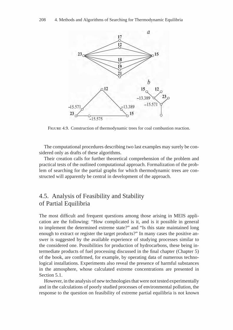
208 4. Methods and Algorithms of Searching for Thermodynamic Equilibria
Figure 4.9. Construction of thermodynamic trees for coal combustion reaction.
The computational procedures describing two last examples may surely be con-sidered only as drafts of these algorithms.
Their creation calls for further theoretical comprehension of the problem andpractical tests of the outlined computational approach. Formalization of the prob-lem of searching for the partial graphs for which thermodynamic trees are con-structed will apparently be central in development of the approach.
4.5. Analysis of Feasibility and Stabilityof Partial Equilibria
The most difficult and frequent questions among those arising in MEIS appli-cation are the following: “How complicated is it, and is it possible in generalto implement the determined extreme state?” and “Is this state maintained longenough to extract or register the target products?” In many cases the positive an-swer is suggested by the available experience of studying processes similar tothe considered one. Possibilities for production of hydrocarbons, these being in-termediate products of fuel processing discussed in the final chapter (Chapter 5)of the book, are confirmed, for example, by operating data of numerous techno-logical installations. Experiments also reveal the presence of harmful substancesin the atmosphere, whose calculated extreme concentrations are presented inSection 5.1.
However, in the analysis of new technologies that were not tested experimentallyand in the calculations of poorly studied processes of environmental pollution, theresponse to the question on feasibility of extreme partial equilibria is not known
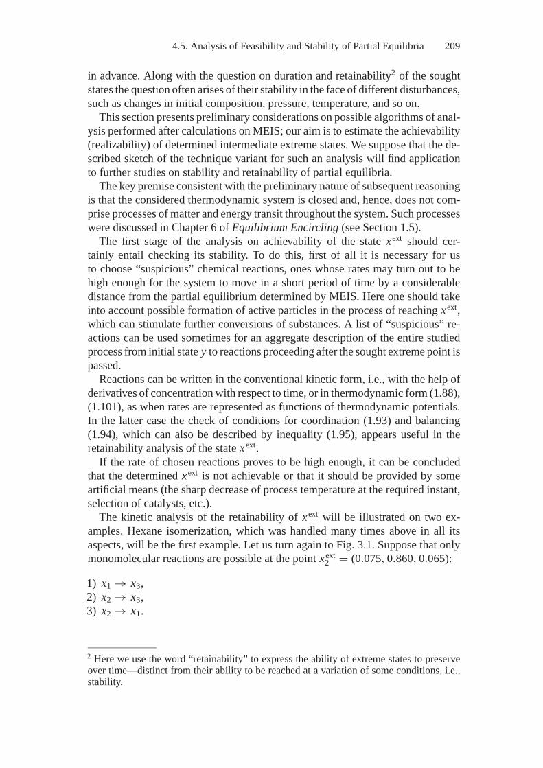
4.5. Analysis of Feasibility and Stability of Partial Equilibria 209
in advance. Along with the question on duration and retainability2 of the soughtstates the question often arises of their stability in the face of different disturbances,such as changes in initial composition, pressure, temperature, and so on.
This section presents preliminary considerations on possible algorithms of anal-ysis performed after calculations on MEIS; our aim is to estimate the achievability(realizability) of determined intermediate extreme states. We suppose that the de-scribed sketch of the technique variant for such an analysis will find applicationto further studies on stability and retainability of partial equilibria.
The key premise consistent with the preliminary nature of subsequent reasoningis that the considered thermodynamic system is closed and, hence, does not com-prise processes of matter and energy transit throughout the system. Such processeswere discussed in Chapter 6 of Equilibrium Encircling (see Section 1.5).
The first stage of the analysis on achievability of the state xext should cer-tainly entail checking its stability. To do this, first of all it is necessary for usto choose “suspicious” chemical reactions, ones whose rates may turn out to behigh enough for the system to move in a short period of time by a considerabledistance from the partial equilibrium determined by MEIS. Here one should takeinto account possible formation of active particles in the process of reaching xext,which can stimulate further conversions of substances. A list of “suspicious” re-actions can be used sometimes for an aggregate description of the entire studiedprocess from initial state y to reactions proceeding after the sought extreme point ispassed.
Reactions can be written in the conventional kinetic form, i.e., with the help ofderivatives of concentration with respect to time, or in thermodynamic form (1.88),(1.101), as when rates are represented as functions of thermodynamic potentials.In the latter case the check of conditions for coordination (1.93) and balancing(1.94), which can also be described by inequality (1.95), appears useful in theretainability analysis of the state xext.
If the rate of chosen reactions proves to be high enough, it can be concludedthat the determined xext is not achievable or that it should be provided by someartificial means (the sharp decrease of process temperature at the required instant,selection of catalysts, etc.).
The kinetic analysis of the retainability of xext will be illustrated on two ex-amples. Hexane isomerization, which was handled many times above in all itsaspects, will be the first example. Let us turn again to Fig. 3.1. Suppose that onlymonomolecular reactions are possible at the point xext
2 = (0.075, 0.860, 0.065):
1) x1 → x3,2) x2 → x3,3) x2 → x1.
2 Here we use the word “retainability” to express the ability of extreme states to preserveover time—distinct from their ability to be reached at a variation of some conditions, i.e.,stability.
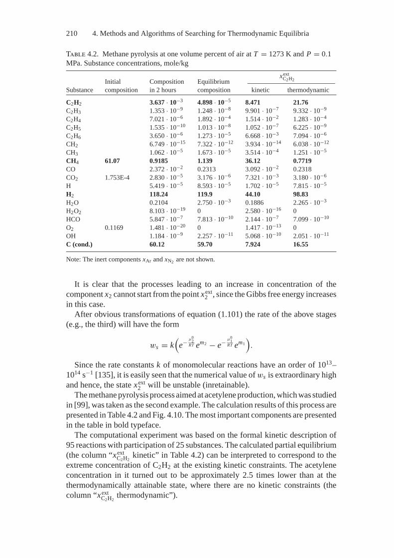
210 4. Methods and Algorithms of Searching for Thermodynamic Equilibria
Table 4.2. Methane pyrolysis at one volume percent of air at T = 1273 K and P = 0.1MPa. Substance concentrations, mole/kg
xextC2H2Initial Composition Equilibrium
Substance composition in 2 hours composition kinetic thermodynamic
C2H2 3.637 · 10−3 4.898 · 10−5 8.471 21.76C2H3 1.353 · 10−9 1.248 · 10−8 9.901 · 10−7 9.332 · 10−9
C2H4 7.021 · 10−6 1.892 · 10−4 1.514 · 10−2 1.283 · 10−4
C2H5 1.535 · 10−10 1.013 · 10−8 1.052 · 10−7 6.225 · 10−9
C2H6 3.650 · 10−6 1.273 · 10−5 6.668 · 10−3 7.094 · 10−6
CH2 6.749 · 10−15 7.322 · 10−12 3.934 · 10−14 6.038 · 10−12
CH3 1.062 · 10−5 1.673 · 10−5 3.514 · 10−4 1.251 · 10−5
CH4 61.07 0.9185 1.139 36.12 0.7719CO 2.372 · 10−2 0.2313 3.092 · 10−2 0.2318CO2 1.753E-4 2.830 · 10−5 3.176 · 10−6 7.321 · 10−3 3.180 · 10−6
H 5.419 · 10−5 8.593 · 10−5 1.702 · 10−5 7.815 · 10−5
H2 118.24 119.9 44.10 98.83H2O 0.2104 2.750 · 10−3 0.1886 2.265 · 10−3
H2O2 8.103 · 10−19 0 2.580 · 10−16 0HCO 5.847 · 10−7 7.813 · 10−10 2.144 · 10−7 7.099 · 10−10
O2 0.1169 1.481 · 10−20 0 1.417 · 10−13 0OH 1.184 · 10−9 2.257 · 10−11 5.068 · 10−10 2.051 · 10−11
C (cond.) 60.12 59.70 7.924 16.55
Note: The inert components xAr and xN2 are not shown.
It is clear that the processes leading to an increase in concentration of thecomponent x2 cannot start from the point xext
2 , since the Gibbs free energy increasesin this case.
After obvious transformations of equation (1.101) the rate of the above stages(e.g., the third) will have the form
ws = k(
e− μ02
RT em2 − e− μ01
RT em1).
Since the rate constants k of monomolecular reactions have an order of 1013–1014 s−1 [135], it is easily seen that the numerical value of ws is extraordinary highand hence, the state xext
2 will be unstable (inretainable).The methane pyrolysis process aimed at acetylene production, which was studied
in [99], was taken as the second example. The calculation results of this process arepresented in Table 4.2 and Fig. 4.10. The most important components are presentedin the table in bold typeface.
The computational experiment was based on the formal kinetic description of95 reactions with participation of 25 substances. The calculated partial equilibrium(the column “xext
C2H2kinetic” in Table 4.2) can be interpreted to correspond to the
extreme concentration of C2H2 at the existing kinetic constraints. The acetyleneconcentration in it turned out to be approximately 2.5 times lower than at thethermodynamically attainable state, where there are no kinetic constraints (thecolumn “xext
C2H2thermodynamic”).
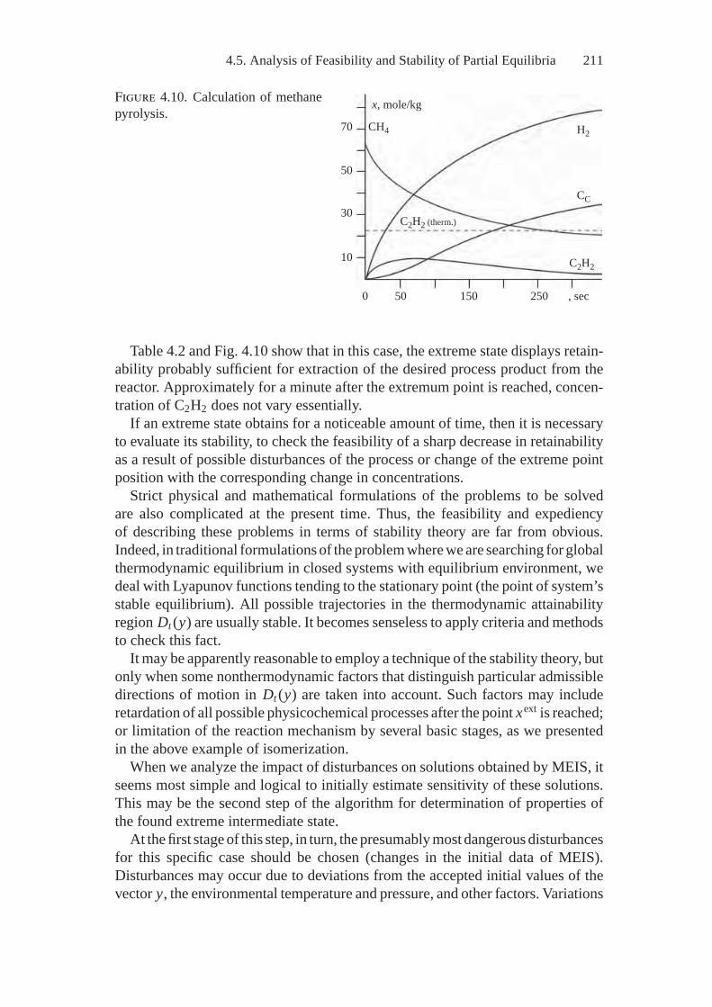
4.5. Analysis of Feasibility and Stability of Partial Equilibria 211
0
10
x, mole/kg
30
50
70 CH4
C2H2 (therm.)
C2H2
CC
H2
50 150 250 , sec
Figure 4.10. Calculation of methanepyrolysis.
Table 4.2 and Fig. 4.10 show that in this case, the extreme state displays retain-ability probably sufficient for extraction of the desired process product from thereactor. Approximately for a minute after the extremum point is reached, concen-tration of C2H2 does not vary essentially.
If an extreme state obtains for a noticeable amount of time, then it is necessaryto evaluate its stability, to check the feasibility of a sharp decrease in retainabilityas a result of possible disturbances of the process or change of the extreme pointposition with the corresponding change in concentrations.
Strict physical and mathematical formulations of the problems to be solvedare also complicated at the present time. Thus, the feasibility and expediencyof describing these problems in terms of stability theory are far from obvious.Indeed, in traditional formulations of the problem where we are searching for globalthermodynamic equilibrium in closed systems with equilibrium environment, wedeal with Lyapunov functions tending to the stationary point (the point of system’sstable equilibrium). All possible trajectories in the thermodynamic attainabilityregion Dt (y) are usually stable. It becomes senseless to apply criteria and methodsto check this fact.
It may be apparently reasonable to employ a technique of the stability theory, butonly when some nonthermodynamic factors that distinguish particular admissibledirections of motion in Dt (y) are taken into account. Such factors may includeretardation of all possible physicochemical processes after the point xext is reached;or limitation of the reaction mechanism by several basic stages, as we presentedin the above example of isomerization.
When we analyze the impact of disturbances on solutions obtained by MEIS, itseems most simple and logical to initially estimate sensitivity of these solutions.This may be the second step of the algorithm for determination of properties ofthe found extreme intermediate state.
At the first stage of this step, in turn, the presumably most dangerous disturbancesfor this specific case should be chosen (changes in the initial data of MEIS).Disturbances may occur due to deviations from the accepted initial values of thevector y, the environmental temperature and pressure, and other factors. Variations
212 4. Methods and Algorithms of Searching for Thermodynamic Equilibria
in the raw material quality (e.g., the composition of fuel burnt in boiler furnaces)is a typical reason for change in technological systems. In natural objects suchchanges can be caused by nonstationary meteorological conditions or unstableanthropogenic loads.
The sensitivity analysis for the selected disturbances can be most easily per-formed by variant calculations on MEIS, determining, for example, the functions� xext = f (�y), where � xext and �y denote changes in the values of the vectorsxext and y with respect to the basic calculated variant.
In the sensitivity analysis the use of the thermodynamic tree may prove to behighly useful. Let us turn again to Fig. 3.1. It is easily seen how the optimal levelof the Gibbs energy G = G(xext) changes as a function of ywhen searching for themaximum concentration of the third component (xext
3 ) of the reaction mixture. Aty = (1, 0, 0)T (vertex 1) this level is equal to −424.118 kJ, and at y = (0, 1, 0)T
(vertex 2) it is −425.678 kJ (Fig. 3.1b). The values of xext3 change correspondingly
(Fig. 3.1a).The last (third) step of the mentioned technique consists apparently in the sta-
bility analysis itself. Some preliminary considerations can also be applied to thisanalysis. For example, it is preferable to use the first (direct) Lyapunov method,since the type and properties of the studied functions are known to a considerableextent beforehand. However, more detailed representation of suppositions on thecontents of the third step is premature yet. In order to exactly formulate the prob-lem solved at this stage we need a sufficient experience in the study on propertiesof extreme partial equilibria.
In conclusion we note that, after the problem of estimating the properties ofextreme states in closed systems is solved successfully (we look to the success), itis necessary to analyze specific features of MEIS-based solutions for open systems.These are, first of all, cases in which transit flows of energy make up an essentialportion of the converted energy in the system, and where modeling of real opensystems by closed ones can lead to significant errors. Here it is convenient to takeadvantage of the approach developed in Chapter 6 of Equilibrium Encircling [58](see Section 1.5).
5Application of Extreme Models
Physicists always have a habit of taking the simplest example of any phenomenon andcalling it “physics”, leaving the more complicated examples to become the concernof other fields—say, of applied mathematics, electrical engineering, chemistry, orcrystallography.
The Feynman lectures on physics
5.1. Thermodynamics of Atmosphere
Objectives of StudyThis section and, indeed, whole chapter are offered to illustrate the use of ex-treme thermodynamic models in applied problems, on the one hand, and to revealthe difficulties arising from such mpdel’s application. We also consider methodseliminating these difficulties.
Capabilities of thermodynamic modeling can be shown by the detailed descrip-tion of the inferences of modeling, explanation of their originality, formulationcomplexity without using thermodynamics principles, usefulness for understand-ing the studied process nature, and elaboration of measures for its improvement.
Presentation of the problems of applying these models implies disclosure ofsecrets of their construction regarding specific features of the object under study;description of computational experiments on their basis and application of othermodels in these experiments and information collected from different sources.
Why is it interesting to analyze air pollution processes to exemplify and illustratethe capabilities of extreme thermodynamic modeling There are several reasons.
First of all, chemical processes in the atmosphere proceed at low temperaturesin comparison with the majority of technological and many other natural pro-cesses. Except for photochemical transformations, they are also characterized byextremely low rates and do not reach a final equilibrium point (see Section 1.4).Live nature and harmful anthropogenic substances in the atmosphere are in partialequilibrium states. This helps explain the skepticism of many specialists concern-ing possible application of thermodynamics to atmospheric chemistry. In terms of
213
214 5. Application of Extreme Models
development of applied thermodynamics and choice of models to study pollutionof the atmosphere and the environment as a whole, it is highly important that weexplain invalidity of such skepticism, doing so by using examples of problems thatwere earlier considered beyond the sphere of thermodynamic analysis.
The next reason to study the air pollution with the help of MEIS is associated withthe complexity of the atmosphere as a thermodynamic system. “Complexity” in thiscase means both a great number of variables influence the values of thermodynamicfunctions, and the corresponding mathematical model is complex with respect toits construction, our analysis of its specific features, and the execution of numericalexperiments on its basis.
The atmosphere is an open heterogeneous system that interacts with the nonequi-librium environment. It comprises a gas phase, as well as water droplets andaerosols (solid and liquid, anthropogenic and natural) [36, 166]. The latter canbe pure condensed substances, but more often they have a heterogeneous spatiallynon-uniform structure, in particular, they are solutions on the surface of solid parti-cles. Both gaseous and condensed matter of the atmosphere is distributed unevenlywith respect to height (mainly due to decrease of air density with height) and onthe horizontal plane (because of air flow).
The nonequilibrium nature of the environment is conditioned by the differenceof temperatures between the aquatic and terrestrial surfaces and radiation (solarand reflected), and also by pressure variation in horizontal direction under theinfluence of heat and mass transfer.
The composition and spatial distribution of substances change in response tohighly diverse physical forces, including chemical affinity, gravity, wind pressure,surface tension, electrical interactions, and others. The transfer processes of energy,substance, and charge that are caused by these forces are often characterized bypronounced irreversibility and have in some cases a clearly defined nonstationarycharacter.
Successful qualitative and quantitative analysis of such a complex system asthe atmosphere using rather simple models is surely the best demonstration of thecompetence and efficiency of thermodynamic idealization of a problem.
Unfortunately, this interest has also been generated by great practical signif-icance of the problem. Air pollution is known to be a major part of the biggerproblem of maintaining life on Earth.
Finally, this example is interesting because the anthropogenic impact on theatmosphere is the subject of very extensive studies on theoretical models and full-scale experiments. And though the results of these studies do not allow a uniqueassessment of the consequences of our current influence on nature, they providerich material for the analysis of thermodynamic modeling results. The informationobtained by nonthermodynamic models and measurements of real atmosphericstates can be used to check correctness of thermodynamic methods for solvingsimilar problems, and to set up schemes for their joint application with kinetic andhydrodynamic models in computational experiments.
We will address three particular problems within the general problem of at-mosphere thermodynamics: 1) assessment of the limiting concentrations of water
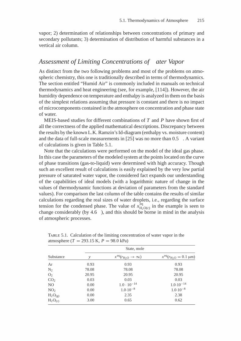
5.1. Thermodynamics of Atmosphere 215
vapor; 2) determination of relationships between concentrations of primary andsecondary pollutants; 3) determination of distribution of harmful substances in avertical air column.
Assessment of Limiting Concentrations of ater VaporAs distinct from the two following problems and most of the problems on atmo-spheric chemistry, this one is traditionally described in terms of thermodynamics.The section entitled “Humid Air” is commonly included in manuals on technicalthermodynamics and heat engineering (see, for example, [114]). However, the airhumidity dependence on temperature and enthalpy is analyzed in them on the basisof the simplest relations assuming that pressure is constant and there is no impactof microcomponents contained in the atmosphere on concentration and phase stateof water.
MEIS-based studies for different combinations of T and P have shown first ofall the correctness of the applied mathematical descriptions. Discrepancy betweenthe results by the known L.K. Ramzin’s Id-diagram (enthalpy vs. moisture content)and the data of full-scale measurements in [25] was no more than 0.5 . A variantof calculations is given in Table 5.1.
Note that the calculations were performed on the model of the ideal gas phase.In this case the parameters of the modeled system at the points located on the curveof phase transitions (gas-to-liquid) were determined with high accuracy. Thoughsuch an excellent result of calculations is easily explained by the very low partialpressure of saturated water vapor, the considered fact expands our understandingof the capabilities of ideal models (with a logarithmic nature of change in thevalues of thermodynamic functions at deviation of parameters from the standardvalues). For comparison the last column of the table contains the results of similarcalculations regarding the real sizes of water droplets, i.e., regarding the surfacetension for the condensed phase. The value of xeq
H2O(c) in the example is seen tochange considerably (by 4.6 ), and this should be borne in mind in the analysisof atmospheric processes.
Table 5.1. Calculation of the limiting concentration of water vapor in theatmosphere (T = 293.15 K, P = 98.0 kPa)
State, mole
Substance y xeq(rH2O → ∞) xeq(rH2O = 0.1 μm)
Ar 0.93 0.93 0.93N2 78.08 78.08 78.08O2 20.95 20.95 20.95CO2 0.03 0.03 0.03NO 0.00 1.0 · 10−14 1.0·10−14
NO2 0.00 1.0·10−8 1.0·10−8
H2O(g) 0.00 2.35 2.38H2O(c) 3.00 0.65 0.62
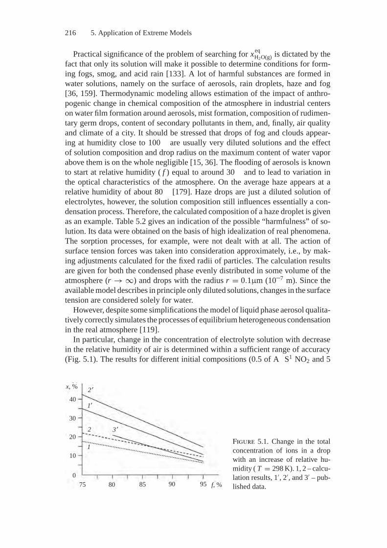
216 5. Application of Extreme Models
Practical significance of the problem of searching for xeqH2O(g) is dictated by the
fact that only its solution will make it possible to determine conditions for form-ing fogs, smog, and acid rain [133]. A lot of harmful substances are formed inwater solutions, namely on the surface of aerosols, rain droplets, haze and fog[36, 159]. Thermodynamic modeling allows estimation of the impact of anthro-pogenic change in chemical composition of the atmosphere in industrial centerson water film formation around aerosols, mist formation, composition of rudimen-tary germ drops, content of secondary pollutants in them, and, finally, air qualityand climate of a city. It should be stressed that drops of fog and clouds appear-ing at humidity close to 100 are usually very diluted solutions and the effectof solution composition and drop radius on the maximum content of water vaporabove them is on the whole negligible [15, 36]. The flooding of aerosols is knownto start at relative humidity ( f ) equal to around 30 and to lead to variation inthe optical characteristics of the atmosphere. On the average haze appears at arelative humidity of about 80 [179]. Haze drops are just a diluted solution ofelectrolytes, however, the solution composition still influences essentially a con-densation process. Therefore, the calculated composition of a haze droplet is givenas an example. Table 5.2 gives an indication of the possible “harmfulness” of so-lution. Its data were obtained on the basis of high idealization of real phenomena.The sorption processes, for example, were not dealt with at all. The action ofsurface tension forces was taken into consideration approximately, i.e., by mak-ing adjustments calculated for the fixed radii of particles. The calculation resultsare given for both the condensed phase evenly distributed in some volume of theatmosphere (r → ∞) and drops with the radius r = 0.1μm (10–7 m). Since theavailable model describes in principle only diluted solutions, changes in the surfacetension are considered solely for water.
However, despite some simplifications the model of liquid phase aerosol qualita-tively correctly simulates the processes of equilibrium heterogeneous condensationin the real atmosphere [119].
In particular, change in the concentration of electrolyte solution with decreasein the relative humidity of air is determined within a sufficient range of accuracy(Fig. 5.1). The results for different initial compositions (0.5 of A S1 NO2 and 5
75 80 85 90 95 f, %
0
10
20
30
40
2 ′
1′
3 ′2
1
x, %
Figure 5.1. Change in the totalconcentration of ions in a dropwith an increase of relative hu-midity ( T = 298 K). 1, 2 – calcu-lation results, 1′, 2′, and 3′ – pub-lished data.
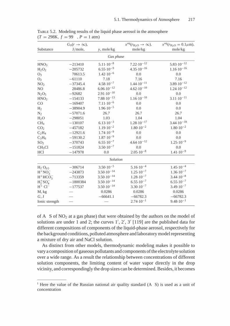
5.1. Thermodynamics of Atmosphere 217
Table 5.2. Modeling results of the liquid phase aerosol in the atmosphere(T = 298K, f = 99 , P = 1 atm)
G0(r → ∞), xeq(rH2O → ∞), xeq(rH2O = 0.1μm),Substance J/mole, y, mole/kg mole/kg mole/kg
Gas phase
HNO3 −213410 5.11·10−8 7.22·10−12 5.83·10−12
H2O2 −205732 6.55·10−9 4.35·10−16 1.16·10−16
O3 70613.5 1.42·10−6 0.0 0.0O2 −61110 7.18 7.16 7.16NO2 −37345.4 4.58·10−7 1.44·10−11 3.89·10−12
NO 28486.8 6.06·10−12 4.62·10−10 1.24·10−12
N2O5 −92682 2.91·10−10 0.0 0.0HNO2 −154133 7.88·10−13 1.16·10−10 3.11·10−11
CO −169407 7.11·10−6 0.0 0.0H2 −38904.9 1.96·10−5 0.0 0.0N2 −57071.6 26.7 26.7 26.7H2O −298051 1.03 1.04 1.04CH4 −130107 6.13·10−3 1.28·10−17 3.44·10−18
CO2 −457182 1.19·10−2 1.80·10−2 1.80·10−2
C2H4 −12921.6 1.74·10−9 0.0 0.0C3H6 −59130.2 1.87·10−9 0.0 0.0SO2 −370743 6.55·10−7 4.64·10−12 1.25·10−9
CH3Cl −151824 3.50·10−7 0.0 0.0HCl −147978 0.0 2.05·10−8 1.41·10−9
Solution
H2 O(c) −306714 3.50·10−5 5.16·10−4 1.45·10−4
H+NO−3 −243873 3.50·10−14 1.25·10−7 1.36·10−7
H+HCO−3 −713359 3.50·10−14 1.28·10−7 3.44·10−8
H+2 SO−
4 −1800384 3.50·10−14 6.55·10−7 6.55·10−7
H+ Cl− −177537 3.50·10−14 3.30·10−7 3.49·10−7
M, kg — 0.0286 0.0286 0.0286G, J — −66641.1 −66782.3 −66782.3Ionic strength — — 2.74·10−1 9.48·10−1
of A S of NO2 at a gas phase) that were obtained by the authors on the model ofsolutions are under 1 and 2; the curves 1′, 2′, 3′ [119] are the published data fordifferent compositions of components of the liquid-phase aerosol, respectively forthe background conditions, polluted atmosphere and laboratory model representinga mixture of dry air and NaCl solution.
As distinct from other models, thermodynamic modeling makes it possible tovary a composition of gaseous pollutants and components of the electrolyte solutionover a wide range. As a result the relationship between concentrations of differentsolution components, the limiting content of water vapor directly in the dropvicinity, and correspondingly the drop sizes can be determined. Besides, it becomes
1 Here the value of the Russian national air quality standard (A S) is used as a unit ofconcentration
218 5. Application of Extreme Models
feasible to study the effect of the initial concentration of gaseous pollutants onsolution composition as well as absorptive capacities of drops with different radii.
The thermodynamic models of change in air humidity are to be applied to thestudy of atmospheric pollution processes and to calculate air conditioning systemsand different-purpose drying installations. In this case, unlike the use of diagrams,we can vary parameters of air composition or drying agent (the latter may containproducts of fuel combustion). The topicality of thermodynamic modeling of airexchange in buildings was shown in Section 3.4.
Analysis of Secondary Atmospheric PollutionThis problem refers to the “illicit” sphere of thermodynamics application, since inthe final equilibrium state the concentrations of the majority of known pollutantsturn out to be some orders of magnitude lower than the admissible ones and arepractically equal to zero, which does not correspond to reality.
Solving the problem requires that we overcome certain numerical difficulties.One of them, i.e., a wide scatter in the values of sought parameters, was discussed inSection 4.3. Another one consists in a great number of primary and secondary pol-lutants and dependence of their conversion reactions in the atmosphere on severalfactors (temperature, air pressure and humidity, solar radiation, etc.). Determi-nation of dependences in formation of many pollutants on different parametersnaturally gives rise to the problem of reducing the number of calculation vari-ants, i.e., the problem of conducting computational experiments. Therefore, thesecondary pollution problem should be discussed starting with the technique ofstudies to be performed.
Its basic point is certainly the choice of an initial thermodynamic model. In thiscase a closed spatially uniform heterogeneous system with a fixed initial compo-sition of reagents that interacts with the environment at the constant T and P wasconsidered. The premise on the system closedness is equivalent to the assumptionthat all processes manage to reach the states of partial or complete equilibria. Thespatial uniformity means that surface tension forces at phase transitions are ne-glected. Assumption of constant temperature and pressure limits the analysis to aground layer of the atmosphere, whose pollution is the most dangerous for natureand humans. With these assumptions made the mathematical formulation of theproblem is apparently reduced to the simplest MEIS modification, i.e., (2.38)–(2.42).
A natural way to decrease the volume of computational experiments is to makea small number of calculations of some typical states and to extend their results toother possible states based on the simplest analytical dependences. Such depen-dences can be determined from the fact that since the atmosphere is an oxidizingmedium, the danger of primary emissions in terms of secondary pollution of theatmosphere is caused to a considerable extent by their reactivity in oxidizationprocesses. Indeed, the energy necessary to drive the reaction of secondary pollu-tant formation may come only from the reactions of primary pollutant oxidation.As far as we consider the system with the constant T and P , the concentration of
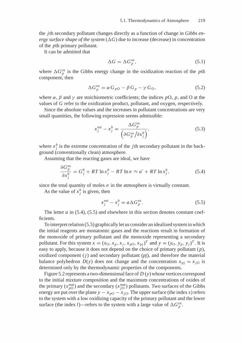
5.1. Thermodynamics of Atmosphere 219
the j th secondary pollutant changes directly as a function of change in Gibbs en-ergy surface shape of the system (�G) due to increase (decrease) in concentrationof the pth primary pollutant.
It can be admitted that
�G = �Goxp , (5.1)
where �Goxp is the Gibbs energy change in the oxidization reaction of the pth
component; then
�Goxp = α G pO − β G p − γ G O , (5.2)
where α, β and γ are stoichiometric coefficients; the indices pO, p, and O at thevalues of G refer to the oxidization product, pollutant, and oxygen, respectively.
Since the absolute values and the increases in pollutant concentrations are verysmall quantities, the following expression seems admissible:
xextj − xb
j = �Goxp(
∂Goxp/∂xb
j
) , (5.3)
where xbj is the extreme concentration of the j th secondary pollutant in the back-
ground (conventionally clean) atmosphere.Assuming that the reacting gases are ideal, we have
∂Goxp
∂xbj
= G0j + RT ln xb
j − RT ln σ ≈ a′ + RT ln xbj , (5.4)
since the total quantity of moles σ in the atmosphere is virtually constant.As the value of xb
j is given, then
xextj − xb
j = a�Goxp . (5.5)
The letter a in (5.4), (5.5) and elsewhere in this section denotes constant coef-ficients.
To interpret relation (5.5) graphically let us consider an idealized system in whichthe initial reagents are monatomic gases and the reactions result in formation ofthe monoxide of primary pollutant and the monoxide representing a secondarypollutant. For this system x = (xO, x p, x j , x pO, x pj )T and y = (yO, yp, y j )T . It iseasy to apply, because it does not depend on the choice of primary pollutant (p),oxidized component ( j) and secondary pollutant (pj), and therefore the materialbalance polyhedron D(y) does not change and the concentration x pj = x jO isdetermined only by the thermodynamic properties of the components.
Figure 5.2 represents a two-dimensional face of D (y) whose vertices correspondto the initial mixture composition and the maximum concentrations of oxides ofthe primary (xmat
pO ) and the secondary (xmatjO ) pollutants. Two surfaces of the Gibbs
energy are put over the plane y − x pO − x jO. The upper surface (the index s) refersto the system with a low oxidizing capacity of the primary pollutant and the lowersurface (the index l)—refers to the system with a large value of �Gox
p .
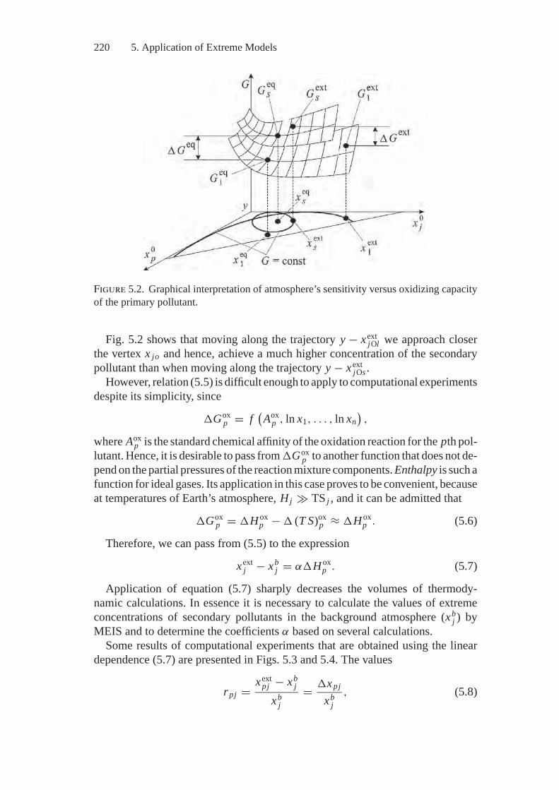
220 5. Application of Extreme Models
Figure 5.2. Graphical interpretation of atmosphere’s sensitivity versus oxidizing capacityof the primary pollutant.
Fig. 5.2 shows that moving along the trajectory y − xextjOl we approach closer
the vertex x jo and hence, achieve a much higher concentration of the secondarypollutant than when moving along the trajectory y − xext
jOs .However, relation (5.5) is difficult enough to apply to computational experiments
despite its simplicity, since
�Goxp = f
(Aox
p , ln x1, . . . , ln xn),
where Aoxp is the standard chemical affinity of the oxidation reaction for the pth pol-
lutant. Hence, it is desirable to pass from �Goxp to another function that does not de-
pend on the partial pressures of the reaction mixture components. Enthalpy is such afunction for ideal gases. Its application in this case proves to be convenient, becauseat temperatures of Earth’s atmosphere, Hj � TS j , and it can be admitted that
�Goxp = �H ox
p − � (T S)oxp ≈ �H ox
p . (5.6)
Therefore, we can pass from (5.5) to the expression
xextj − xb
j = α�H oxp . (5.7)
Application of equation (5.7) sharply decreases the volumes of thermody-namic calculations. In essence it is necessary to calculate the values of extremeconcentrations of secondary pollutants in the background atmosphere (xb
j ) byMEIS and to determine the coefficients α based on several calculations.
Some results of computational experiments that are obtained using the lineardependence (5.7) are presented in Figs. 5.3 and 5.4. The values
rpj = xextpj − xb
j
xbj
= �x pj
xbj
, (5.8)
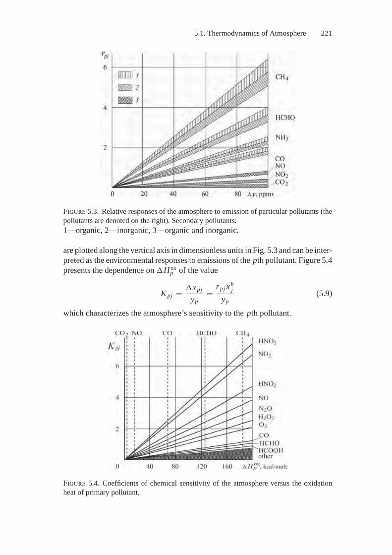
5.1. Thermodynamics of Atmosphere 221
Figure 5.3. Relative responses of the atmosphere to emission of particular pollutants (thepollutants are denoted on the right). Secondary pollutants:1—organic, 2—inorganic, 3—organic and inorganic.
are plotted along the vertical axis in dimensionless units in Fig. 5.3 and can be inter-preted as the environmental responses to emissions of the pth pollutant. Figure 5.4presents the dependence on �H ox
p of the value
K pj = �x pj
yp= rpj xb
j
yp(5.9)
which characterizes the atmosphere’s sensitivity to the pth pollutant.
Figure 5.4. Coefficients of chemical sensitivity of the atmosphere versus the oxidationheat of primary pollutant.
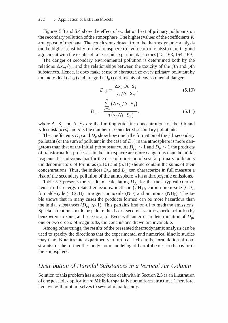
222 5. Application of Extreme Models
Figures 5.3 and 5.4 show the effect of oxidation heat of primary pollutants onthe secondary pollution of the atmosphere. The highest values of the coefficients Kare typical of methane. The conclusions drawn from the thermodynamic analysison the higher sensitivity of the atmosphere to hydrocarbon emission are in goodagreement with the results of kinetic and experimental studies [12, 163, 164, 169].
The danger of secondary environmental pollution is determined both by therelations �x pj/yp and the relationships between the toxicity of the j th and pthsubstances. Hence, it does make sense to characterize every primary pollutant bythe individual (Dpj ) and integral (Dp) coefficients of environmental danger:
Dpj = �xpj/A S j
yp/A Sp, (5.10)
Dp =
n∑j=1
(�xpj/A S j
)n(yp/A Sp
) , (5.11)
where A S j and A Sp are the limiting guideline concentrations of the j th andpth substances; and n is the number of considered secondary pollutants.
The coefficients Dpj and Dp show how much the formation of the j th secondarypollutant (or the sum of pollutant in the case of Dp) in the atmosphere is more dan-gerous than that of the initial pth substance. At Dpj > 1 and Dp > 1 the productsof transformation processes in the atmosphere are more dangerous than the initialreagents. It is obvious that for the case of emission of several primary pollutantsthe denominators of formulas (5.10) and (5.11) should contain the sums of theirconcentrations. Thus, the indices Dpj and Dp can characterize in full measure arisk of the secondary pollution of the atmosphere with anthropogenic emissions.
Table 5.3 presents the results of calculating Dpj for the most typical compo-nents in the energy-related emissions: methane (CH4), carbon monoxide (CO),formaldehyde (HCOH), nitrogen monoxide (NO) and ammonia (NH3). The ta-ble shows that in many cases the products formed can be more hazardous thanthe initial substances (Dpj � 1). This pertains first of all to methane emissions.Special attention should be paid to the risk of secondary atmospheric pollution bybenzpyrene, ozone, and prussic acid. Even with an error in determination of Dpjone or two orders of magnitude, the conclusions drawn are invariable.
Among other things, the results of the presented thermodynamic analysis can beused to specify the directions that the experimental and numerical kinetic studiesmay take. Kinetics and experiments in turn can help in the formulation of con-straints for the further thermodynamic modeling of harmful emission behavior inthe atmosphere.
Distribution of Harmful Substances in a Vertical Air ColumnSolution to this problem has already been dealt with in Section 2.3 as an illustrationof one possible application of MEIS for spatially nonuniform structures. Therefore,here we will limit ourselves to several remarks only.
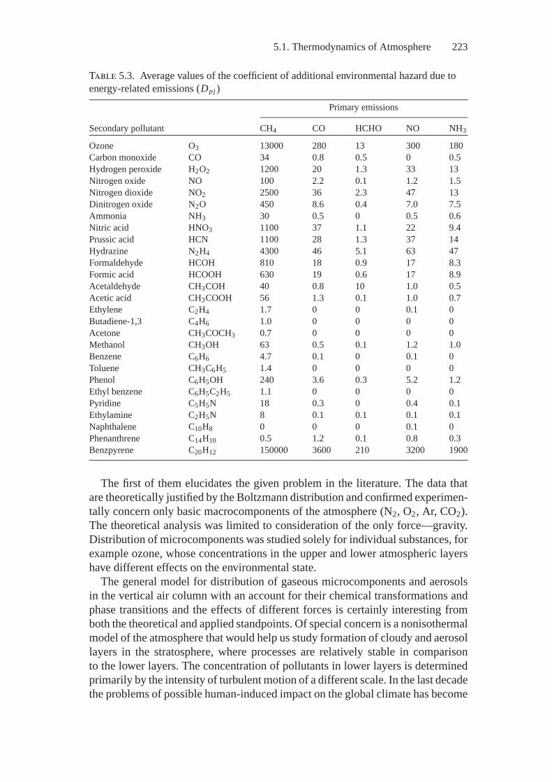
5.1. Thermodynamics of Atmosphere 223
Table 5.3. Average values of the coefficient of additional environmental hazard due toenergy-related emissions (Dpj )
Primary emissions
Secondary pollutant CH4 CO HCHO NO NH3
Ozone O3 13000 280 13 300 180Carbon monoxide CO 34 0.8 0.5 0 0.5Hydrogen peroxide H2O2 1200 20 1.3 33 13Nitrogen oxide NO 100 2.2 0.1 1.2 1.5Nitrogen dioxide NO2 2500 36 2.3 47 13Dinitrogen oxide N2O 450 8.6 0.4 7.0 7.5Ammonia NH3 30 0.5 0 0.5 0.6Nitric acid HNO3 1100 37 1.1 22 9.4Prussic acid HCN 1100 28 1.3 37 14Hydrazine N2H4 4300 46 5.1 63 47Formaldehyde HCOH 810 18 0.9 17 8.3Formic acid HCOOH 630 19 0.6 17 8.9Acetaldehyde CH3COH 40 0.8 10 1.0 0.5Acetic acid CH3COOH 56 1.3 0.1 1.0 0.7Ethylene C2H4 1.7 0 0 0.1 0Butadiene-1,3 C4H6 1.0 0 0 0 0Acetone CH3COCH3 0.7 0 0 0 0Methanol CH3OH 63 0.5 0.1 1.2 1.0Benzene C6H6 4.7 0.1 0 0.1 0Toluene CH3C6H5 1.4 0 0 0 0Phenol C6H5OH 240 3.6 0.3 5.2 1.2Ethyl benzene C6H5C2H5 1.1 0 0 0 0Pyridine C5H5N 18 0.3 0 0.4 0.1Ethylamine C2H5N 8 0.1 0.1 0.1 0.1Naphthalene C10H8 0 0 0 0.1 0Phenanthrene C14H10 0.5 1.2 0.1 0.8 0.3Benzpyrene C20H12 150000 3600 210 3200 1900
The first of them elucidates the given problem in the literature. The data thatare theoretically justified by the Boltzmann distribution and confirmed experimen-tally concern only basic macrocomponents of the atmosphere (N2, O2, Ar, CO2).The theoretical analysis was limited to consideration of the only force—gravity.Distribution of microcomponents was studied solely for individual substances, forexample ozone, whose concentrations in the upper and lower atmospheric layershave different effects on the environmental state.
The general model for distribution of gaseous microcomponents and aerosolsin the vertical air column with an account for their chemical transformations andphase transitions and the effects of different forces is certainly interesting fromboth the theoretical and applied standpoints. Of special concern is a nonisothermalmodel of the atmosphere that would help us study formation of cloudy and aerosollayers in the stratosphere, where processes are relatively stable in comparisonto the lower layers. The concentration of pollutants in lower layers is determinedprimarily by the intensity of turbulent motion of a different scale. In the last decadethe problems of possible human-induced impact on the global climate has become
224 5. Application of Extreme Models
extremely topical. An important aspect of the problem is to assess a role of thetroposphere and stratospheric aerosol in the processes of scatter and reflectionof short- and long-wave radiation and also condensation, i.e., formation of thecloud cover [1]. The most difficult problem here is determining the contribution ofanthropogenic particles or the indirect human-induced effect on aerosol formationand transfer and on atmospheric chemistry in general [11]. The thermodynamicmodel of the vertical air column would possibly assist in revealing some lawsconcerning specific features in formation of the aerosol layers regarding theirdispersion and chemical composition.
Depending on the objectives of the study, the thermodynamic modeling canexamine different column heights at different steps in the vertical plane. Variationof the sizes and structure of cells in the modeled system provides an idea ofboth distribution of harmful substances in the ground layer of the atmosphere(under certain conditions) and processes extending over the whole column of thetroposphere and even in the middle atmosphere.
It was shown in [92] that MEIS for spatially inhomogeneous structures could beapplied to the analysis of substance distribution over the horizontal plane as well.In this case, terrain relief and other factors can be taken into consideration.
Application of spatial thermodynamic models in combination with models ofchemical kinetics and transfer (motion induced by pressure drop, molecular andturbulent diffusion, heat exchange) proves to be the most effective. Increase in thenumber of quite different models to describe one and the same system we maysuppose will give a deeper insight into the processes occurring in that system andlead to accurate forecasting of processes’ results.
5.2. Thermodynamics of Combustion
ntroductory otesUnlike atmospheric chemistry, the chemistry of combustion was not a forbiddenarea for thermodynamic analysis. As was mentioned in the Introduction (Sec-tion I.23), the main features of hydrogen combustion thermodynamics were dis-covered by D. Gibbs. Now the thermodynamic interpretations of oxidation of themain combustible components in fossil fuel are clear. However, currently, envi-ronmental characteristics of furnaces and combustion chambers are studied almostsolely by kinetic models and full-scale experiments. And the necessity for thermo-dynamic methods to penetrate into this sphere of studies has yet to be demonstrated.In this section of the book the authors make one more attempt (the previous onesare presented, e.g., in [50, 80, 81]) to explain a certain technique of using thermo-dynamic models and reveal the model’s effectiveness for the analysis of harmfulsubstances formed at fuel burning.
In terms of revealing the capabilities of thermodynamics, the processes of bothcombustion and atmospheric pollution are highly interesting because of their com-plexity and great practical significance. Besides, the available abundant data on
5.2. Thermodynamics of Combustion 225
release of pollutants during fuel burning allows the estimation of thermodynamicmodeling accuracy and facilitates elaboration of algorithms of joint applicationof the kinetic and thermodynamic models and full-scale experiments to studyphysicochemical processes. We now describe the factors determining the scien-tific significance of combustion thermodynamics in greater detail.
Fuel is burnt in open systems with a nonequilibrium environment. Mass isexchanged with the latter by flows of fuel, air (oxidant), recirculating and flue gases,slag, and ash of different temperature. As a rule these systems are heterogeneous.Heterogeneity proves to be highest at solid fuel combustion, first among thesebeing coals that consist of both organic and diverse mineral matter. Reactions withparticipation of the mineral part of fuel can result in formation of gaseous andcondensed compounds. The number of reaction mixture components may reachmany hundreds. Design of a combustion appliance and the arrangement of fuelburning in it stipulate both chemical and other interactions: mechanical, thermal,gravitational, electrical and electromagnetic, and radiative.
Periodic processes of fuel combustion at small boiler plants and furnaces are notsteady. However, insteadiness is most typical of operation of transport engines. Arevelation of the specific features of such complex real objects by comparativelysimple models of equilibria seems highly instructive to the task of mastering theart of thermodynamic modeling.
The practical importance of environmental analysis of fuel combustion pro-cesses, it being a key source of pollution in nature, requires no comment. Ther-modynamics, however, allows both estimation of the potential negative impact ofproduction installations on the environment and determination of the factors influ-encing the reliability and security of equipment operation. Thermodynamic studieson slag formation at water pipes of furnaces, as well as sulfuric acid corrosion ofthe rear heating surfaces of boiler units, are examples of problems related to thereliability problem. We may recall the practical significance of such traditionalthermodynamic analysis applied in the energy sector for determining specific fuelconsumption for production processes.
Combustion is a better illustration than atmospheric pollution, when we tendto compare thermodynamic models to kitetic models and full-scale experiments.In human-organized processes as compared to natural ones, it is much easier todetermine initial system state, conditions of interaction with the environment, andpossible ranges of initial data variation. When we study atmospheric pollutionit turns out to be rather difficult to estimate composition prior to anthropogenicimpacts and the extent of these impacts (emissions of harmful substances). It isextremely difficult to take into account the effect of infinitely diverse natural factors(solar radiation, air flows, mass exchange with water and ground surfaces, etc.) onall the microcomponents present in the atmosphere.
A wide experience has been gained by now on MEIS application to the analysisof combustion processes for different types of coals, heavy oil, gas, productionwaste, designs of boiler furnaces and stoves, and furnace regimes. Environ-mental characteristics of energy and public utility installations for fuel com-bustion have been studied to the greatest extent [50, 81, 138]. Nonequilibrium
226 5. Application of Extreme Models
plasma ignition and lightening of pulverized-coal torches have been alsoanalyzed.
Here we will dwell on only two problems: 1) analysis of nitrogen oxide formationat coal combustion; and 2) study of the environmental characteristics of periodicprocesses of solid fuel combustion at small boiler plants and stoves.
Theoretically interesting issues of MEIS application to the study of nonequilib-rium plasma processes are considered briefly in the next section.
Thermodynamic Modeling of itrogen Oxides Formationin Coal FurnacesThe processes of NOx formation at fuel combustion have long been the subject ofsystematic studies for many specialists in different countries [48, 147, 165, 169,176]. Such studies resulted in accumulation of a wide range of experimental data.There are theoretical achievements and practical recommendations, and many ofthem have already been implemented. However, many problems call for furtherinvestigation in this sphere. They are, for example, raising the efficiency of tech-nologies for NOx emission reduction, evaluation of the potential for improvingthese technologies, prevention from formation of other harmful substances due toNOx suppression, and so on.
MEIS was used for the thermodynamic analysis of forming thermal, fuel, andprompt nitrogen oxides 2 at coal combustion [50, 81]. The analysis was made on theKansk–Achinsk coal of the Irsha–Borodinsk deposit. The conventional chemicalformula for the organic mass of this coal has the form: CH0.833O0.233N0.012S0.002.The greatest efforts were made to study dependences of the NOx concentration ona) thermodynamic parameters, b) the composition of the reaction mixture, c) theprocess mechanism, and d) conditions of energy and mass exchange.
In the analysis the general MEIS was the basis for constructing models repre-senting a real combustion process in sufficient detail and those employing utmostidealization of the mechanism of chemical reactions. The most detailed modelcomprised 200 components formed by 12 chemical elements. Coal’s organic andmineral parts were presented. The vector x included 50 gaseous and condensednitrogen compounds along with sulfur compounds, hydrocarbons, heavy metals,and other substances. Studies on reaction mixtures with such a wide compositionof substances by kinetic modeling gives rise to many difficulties.
The results of calculation of equilibrium concentrations of nitrogen compounds(at the point xeq) with the air excess coefficient3 αair = 1.2 obtained by the de-tailed model are presented in Fig. 5.5. Nitrogen monoxide (NO) prevails amongthese compounds, which agrees with experimental data. Figure 5.6 illustrates
2 Thermal oxides are formed at fuel burning from atmospheric nitrogen and oxygen. Fueloxides are the result of oxidation of nitrogen-containing compounds of coal. Prompt oxidesare formed from atmospheric nitrogen as a result of its interaction with active speciesemerging at thermal destruction of the organic part of fuel.3 The ratio between the available air and the stoichiometrically needed amount of it.
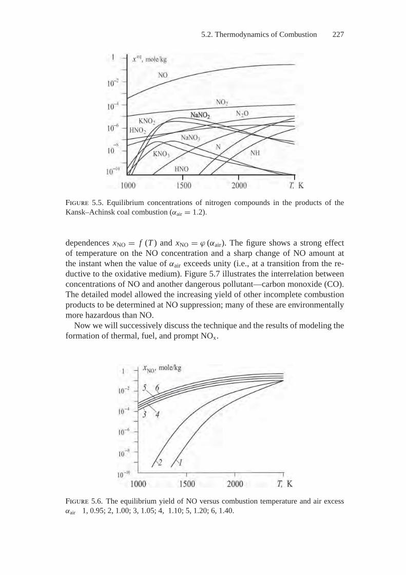
5.2. Thermodynamics of Combustion 227
Figure 5.5. Equilibrium concentrations of nitrogen compounds in the products of theKansk–Achinsk coal combustion (αair = 1.2).
dependences xNO = f (T ) and xNO = ϕ (αair). The figure shows a strong effectof temperature on the NO concentration and a sharp change of NO amount atthe instant when the value of αair exceeds unity (i.e., at a transition from the re-ductive to the oxidative medium). Figure 5.7 illustrates the interrelation betweenconcentrations of NO and another dangerous pollutant—carbon monoxide (CO).The detailed model allowed the increasing yield of other incomplete combustionproducts to be determined at NO suppression; many of these are environmentallymore hazardous than NO.
Now we will successively discuss the technique and the results of modeling theformation of thermal, fuel, and prompt NOx.
Figure 5.6. The equilibrium yield of NO versus combustion temperature and air excessαair 1, 0.95; 2, 1.00; 3, 1.05; 4, 1.10; 5, 1.20; 6, 1.40.
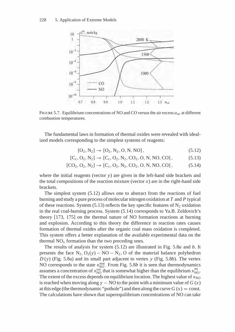
228 5. Application of Extreme Models
Figure 5.7. Equilibrium concentrations of NO and CO versus the air excess αair at differentcombustion temperatures.
The fundamental laws in formation of thermal oxides were revealed with ideal-ized models corresponding to the simplest systems of reagents:
[O2, N2] → [O2, N2, O, N, NO] , (5.12)[Cc, O2, N2] → [Cc, O2, N2, CO2, O, N, NO, CO] , (5.13)
[CO2, O2, N2] → [Cc, O2, N2, CO2, O, N, NO, CO] , (5.14)
where the initial reagents (vector y) are given in the left-hand side brackets andthe total compositions of the reaction mixture (vector x) are in the right-hand sidebrackets.
The simplest system (5.12) allows one to abstract from the reactions of fuelburning and study a pure process of molecular nitrogen oxidation at T and P typicalof these reactions. System (5.13) reflects the key specific features of N2 oxidationin the real coal-burning process. System (5.14) corresponds to Ya.B. Zeldovich’stheory [173, 175] on the thermal nature of NO formation reactions at burningand explosion. According to this theory the difference in reaction rates causesformation of thermal oxides after the organic coal mass oxidation is completed.This system offers a better explanation of the available experimental data on thethermal NOx formation than the two preceding ones.
The results of analysis for system (5.12) are illustrated in Fig. 5.8a and b. Itpresents the face N2, O2(y) − NO − N2, O of the material balance polyhedronD (y) (Fig. 5.8a) and its small part adjacent to vertex y (Fig. 5.8b). The vertexNO corresponds to the state xmat
NO . From Fig. 5.8b it is seen that thermodynamicsassumes a concentration of xext
NO that is somewhat higher than the equilibrium xeqNO.
The extent of the excess depends on equilibrium location. The highest value of xNOis reached when moving along y − NO to the point with a minimum value of G (x)at this edge (the thermodynamic “pothole”) and then along the curve G (x) = const.The calculations have shown that superequilibrium concentrations of NO can take
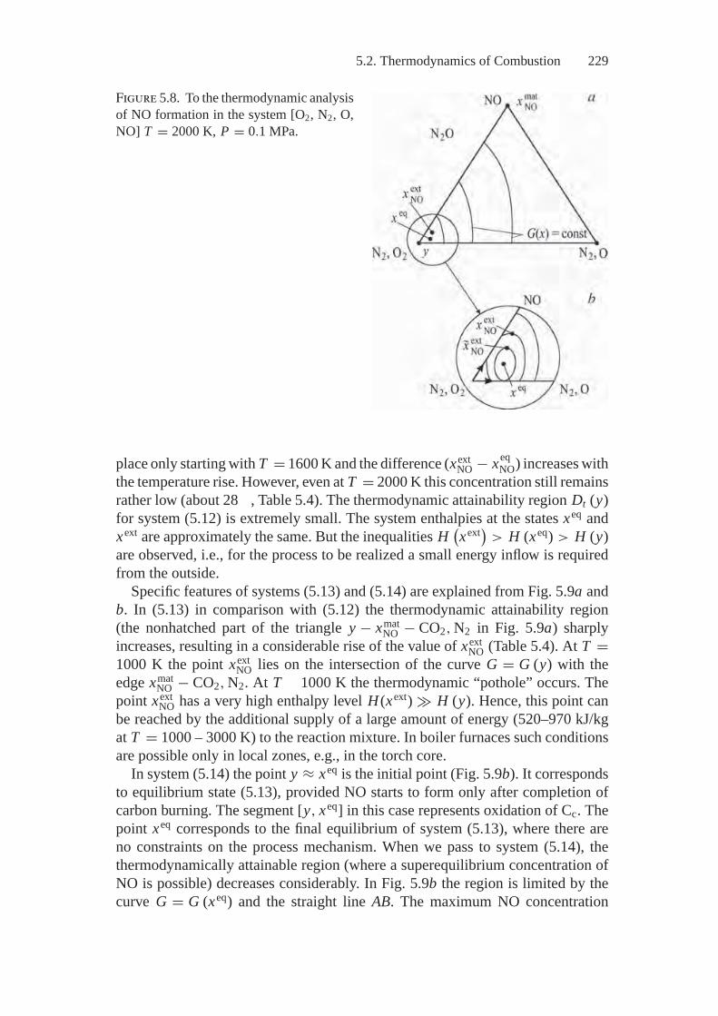
5.2. Thermodynamics of Combustion 229
Figure 5.8. To the thermodynamic analysisof NO formation in the system [O2, N2, O,NO] T = 2000 K, P = 0.1 MPa.
place only starting with T = 1600 K and the difference (xextNO − xeq
NO) increases withthe temperature rise. However, even at T = 2000 K this concentration still remainsrather low (about 28 , Table 5.4). The thermodynamic attainability region Dt (y)for system (5.12) is extremely small. The system enthalpies at the states xeq andxext are approximately the same. But the inequalities H
(xext) > H (xeq) > H (y)
are observed, i.e., for the process to be realized a small energy inflow is requiredfrom the outside.
Specific features of systems (5.13) and (5.14) are explained from Fig. 5.9a andb. In (5.13) in comparison with (5.12) the thermodynamic attainability region(the nonhatched part of the triangle y − xmat
NO − CO2, N2 in Fig. 5.9a) sharplyincreases, resulting in a considerable rise of the value of xext
NO (Table 5.4). At T =1000 K the point xext
NO lies on the intersection of the curve G = G (y) with theedge xmat
NO − CO2, N2. At T 1000 K the thermodynamic “pothole” occurs. Thepoint xext
NO has a very high enthalpy level H (xext) � H (y). Hence, this point canbe reached by the additional supply of a large amount of energy (520–970 kJ/kgat T = 1000 – 3000 K) to the reaction mixture. In boiler furnaces such conditionsare possible only in local zones, e.g., in the torch core.
In system (5.14) the point y ≈ xeq is the initial point (Fig. 5.9b). It correspondsto equilibrium state (5.13), provided NO starts to form only after completion ofcarbon burning. The segment [y, xeq] in this case represents oxidation of Cc. Thepoint xeq corresponds to the final equilibrium of system (5.13), where there areno constraints on the process mechanism. When we pass to system (5.14), thethermodynamically attainable region (where a superequilibrium concentration ofNO is possible) decreases considerably. In Fig. 5.9b the region is limited by thecurve G = G (xeq) and the straight line AB. The maximum NO concentration
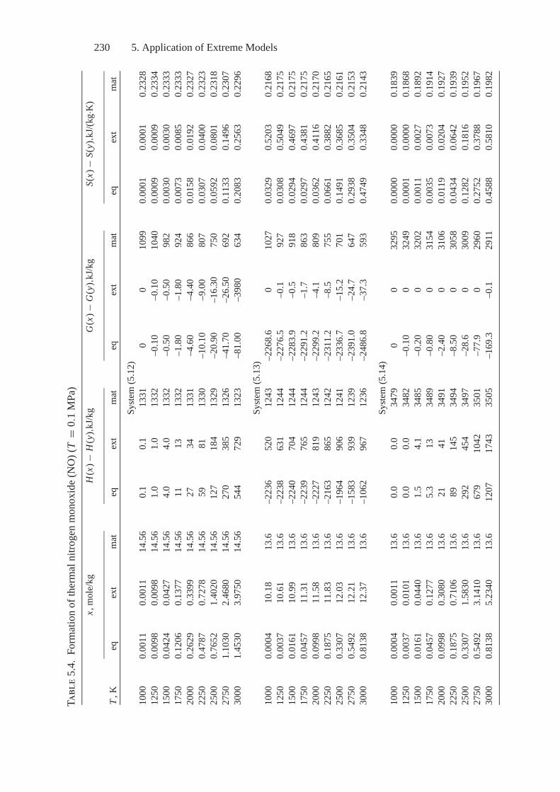
230 5. Application of Extreme Models
Tabl
e5.
4.Fo
rmat
ion
ofth
erm
alni
troge
nm
onox
ide(
NO
)(T
=0.
1M
Pa)
x,m
ole/
kgH
(x)−
H(y
),kJ/k
gG
(x)−
G(y
),kJ/k
gS(
x)−
S(y)
,kJ/(
kg·K
)
T,K
eqex
tm
ateq
ext
mat
eqex
tm
ateq
ext
mat
Syste
m(5
.12)
1000
0.00
110.
0011
14.5
60.
10.
113
310
010
990.
0001
0.00
010.
2328
1250
0.00
980.
0098
14.5
61.
01.
013
32–0
.10
–0.1
010
400.
0009
0.00
090.
2334
1500
0.04
240.
0427
14.5
64.
04.
013
32–0
.50
–0.5
098
20.
0030
0.00
300.
2333
1750
0.12
060.
1377
14.5
611
1313
32–1
.80
–1.8
092
40.
0073
0.00
850.
2333
2000
0.26
290.
3399
14.5
627
3413
31–4
.60
–4.4
086
60.
0158
0.01
920.
2327
2250
0.47
870.
7278
14.5
659
8113
30–1
0.10
–9.0
080
70.
0307
0.04
000.
2323
2500
0.76
521.
4020
14.5
612
718
413
29–2
0.90
–16.
3075
00.
0592
0.08
010.
2318
2750
1.10
302.
4680
14.5
627
038
513
26–4
1.70
–26.
5069
20.
1133
0.14
960.
2307
3000
1.45
303.
9750
14.5
654
472
913
23–8
1.00
–398
063
40.
2083
0.25
630.
2296
Syste
m(5
.13)
1000
0.00
0410
.18
13.6
–223
652
012
43–2
268.
60
1027
0.03
290.
5203
0.21
6812
500.
0037
10.6
113
.6–2
238
631
1244
–227
6.5
–0.1
927
0.03
080.
5049
0.21
7515
000.
0161
10.9
913
.6–2
240
704
1244
–228
3.9
–0.5
918
0.02
940.
4697
0.21
7517
500.
0457
11.3
113
.6–2
239
765
1244
–229
1.2
–1.7
863
0.02
970.
4381
0.21
7520
000.
0998
11.5
813
.6–2
227
819
1243
–229
9.2
–4.1
809
0.03
620.
4116
0.21
7022
500.
1875
11.8
313
.6–2
163
865
1242
–231
1.2
–8.5
755
0.06
610.
3882
0.21
6525
000.
3307
12.0
313
.6–1
964
906
1241
–233
6.7
–15.
270
10.
1491
0.36
850.
2161
2750
0.54
9212
.21
13.6
–158
393
912
39–2
391.
0–2
4.7
647
0.29
380.
3504
0.21
5330
000.
8138
12.3
713
.6–1
062
967
1236
–248
6.8
–37.
359
30.
4749
0.33
480.
2143
Syste
m(5
.14)
1000
0.00
040.
0011
13.6
0.0
0.0
3479
00
3295
0.00
000.
0000
0.18
3912
500.
0037
0.01
0113
.60.
00.
034
82–0
.10
032
490.
0001
0.00
000.
1868
1500
0.01
610.
0440
13.6
1.5
4.1
3485
–0.2
00
3202
0.00
110.
0027
0.18
9217
500.
0457
0.12
7713
.65.
313
3489
–0.8
00
3154
0.00
350.
0073
0.19
1420
000.
0998
0.30
8013
.621
4134
91–2
.40
031
060.
0119
0.02
040.
1927
2250
0.18
750.
7106
13.6
8914
534
94–8
.50
030
580.
0434
0.06
420.
1939
2500
0.33
071.
5830
13.6
292
454
3497
–28.
60
3009
0.12
820.
1816
0.19
5227
500.
5492
3.14
1013
.667
910
4235
01–7
7.9
029
600.
2752
0.37
880.
1967
3000
0.81
385.
2340
13.6
1207
1743
3505
–169
.3–0
.129
110.
4588
0.58
100.
1982
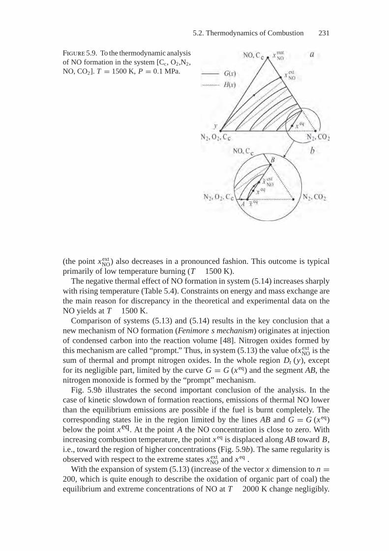
5.2. Thermodynamics of Combustion 231
Figure 5.9. To the thermodynamic analysisof NO formation in the system [Cc, O2,N2,NO, CO2]. T = 1500 K, P = 0.1 MPa.
(the point xextNO) also decreases in a pronounced fashion. This outcome is typical
primarily of low temperature burning (T 1500 K).The negative thermal effect of NO formation in system (5.14) increases sharply
with rising temperature (Table 5.4). Constraints on energy and mass exchange arethe main reason for discrepancy in the theoretical and experimental data on theNO yields at T 1500 K.
Comparison of systems (5.13) and (5.14) results in the key conclusion that anew mechanism of NO formation (Fenimore s mechanism) originates at injectionof condensed carbon into the reaction volume [48]. Nitrogen oxides formed bythis mechanism are called “prompt.” Thus, in system (5.13) the value ofxext
NO is thesum of thermal and prompt nitrogen oxides. In the whole region Dt (y), exceptfor its negligible part, limited by the curve G = G (xeq) and the segment AB, thenitrogen monoxide is formed by the “prompt” mechanism.
Fig. 5.9b illustrates the second important conclusion of the analysis. In thecase of kinetic slowdown of formation reactions, emissions of thermal NO lowerthan the equilibrium emissions are possible if the fuel is burnt completely. Thecorresponding states lie in the region limited by the lines AB and G = G (xeq)below the point xeq. At the point A the NO concentration is close to zero. Withincreasing combustion temperature, the point xeq is displaced along AB toward B,i.e., toward the region of higher concentrations (Fig. 5.9b). The same regularity isobserved with respect to the extreme states xext
NO and xeq .With the expansion of system (5.13) (increase of the vector x dimension to n =
200, which is quite enough to describe the oxidation of organic part of coal) theequilibrium and extreme concentrations of NO at T 2000 K change negligibly.
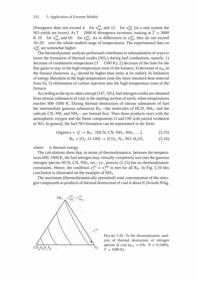
232 5. Application of Extreme Models
Divergence does not exceed 4 for xeqNO and 15 for xext
NO (in a real system theNO yields are lower). At T 2000 K divergence increases, making at T = 3000K 10 for xeq
NO and 60 for xextNO. As to differences in xext
NO, they do not exceed10–20 over the whole studied range of temperatures. The experimental data onxext
NO are somewhat higher.The thermodynamic analysis performed contributes to substantiation of ways to
lower the formation of thermal oxides (NOx) during fuel combustion, namely: 1)decrease of combustion temperature (T 1500 K); 2) decrease of the time for theflue gases to stay in the high temperature zone of the furnace; 3) decrease of αair inthe furnace (however, αair should be higher than unity at its outlet); 4) limitationof energy liberation in the high-temperature zone (by more intensive heat removalfrom it); 5) elimination of carbon injection into the high-temperature zone of thefurnace.
According to the up-to-date concept [147, 165], fuel nitrogen oxides are obtainedfrom nitrous substances of coal in the starting section of torch, when temperaturesreaches 900–1000 K. During thermal destruction of nitrous substances of fuelthe intermediate gaseous substances RN—the molecules of HCN, NH3, and theradicals CN, NH, and NH2—are formed first. Then these products react with theatmospheric oxygen and the flame components O and OH with partial oxidationto NO. In general, the fuel NO formation can be represented in the form:
Organics + Q → RN : [HCN, CN, NH3, NH2, . . .], (5.15)RN + [O2, O, OH] → [CO2, N2, NO, H2O], (5.16)
where is thermal energy.The calculations show that, in terms of thermodynamics, between the tempera-
tures 600–1000 K, the fuel nitrogen may virtually completely turn into the gaseousnitrogen species HCN, CN, NH3, etc.; i.e., process (5.15) has no thermodynamicconstraints. Hence, the condition xext
j = xmatj is met for all RN. In Fig. 5.10 this
conclusion is illustrated on the example of NH3.The maximum (thermodynamically permitted) total concentration of the nitro-
gen compounds in products of thermal destruction of coal is about 0.24 mole N/kg.
Figure 5.10. To the thermodynamic anal-ysis of thermal destruction of nitrogenspecies of coal (αair = 0.8; P = 0.1MPa,T = 1000 K).
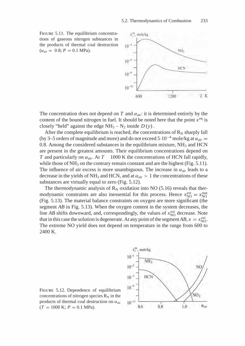
5.2. Thermodynamics of Combustion 233
Figure 5.11. The equilibrium concentra-tions of gaseous nitrogen substances inthe products of thermal coal destruction(αair = 0.8; P = 0.1 MPa).
The concentration does not depend on T and αair: it is determined entirely by thecontent of the bound nitrogen in fuel. It should be noted here that the point xeq isclosely “held” against the edge NH3 – N2 inside D (y) .
After the complete equilibrium is reached, the concentrations of RN sharply fall(by 3–5 orders of magnitude and more) and do not exceed 5·10−4 mole/kg at αair =0.8. Among the considered substances in the equilibrium mixture, NH3 and HCNare present in the greatest amounts. Their equilibrium concentrations depend onT and particularly on αair. At T 1000 K the concentrations of HCN fall rapidly,while those of NH3 on the contrary remain constant and are the highest (Fig. 5.11).The influence of air excess is more unambiguous. The increase in αair leads to adecrease in the yields of NH3 and HCN, and at αair > 1 the concentrations of thesesubstances are virtually equal to zero (Fig. 5.12).
The thermodynamic analysis of RN oxidation into NO (5.16) reveals that ther-modynamic constraints are also inessential for this process. Hence xext
NO = xmatNO
(Fig. 5.13). The material balance constraints on oxygen are more significant (thesegment AB in Fig. 5.13). When the oxygen content in the system decreases, theline AB shifts downward, and, correspondingly, the values of xext
NO decrease. Notethat in this case the solution is degenerate. At any point of the segment AB, x = xext
NO.The extreme NO yield does not depend on temperature in the range from 600 to2400 K.
Figure 5.12. Dependence of equilibriumconcentrations of nitrogen species RN in theproducts of thermal coal destruction on αair(T = 1000 K; P = 0.1 MPa).
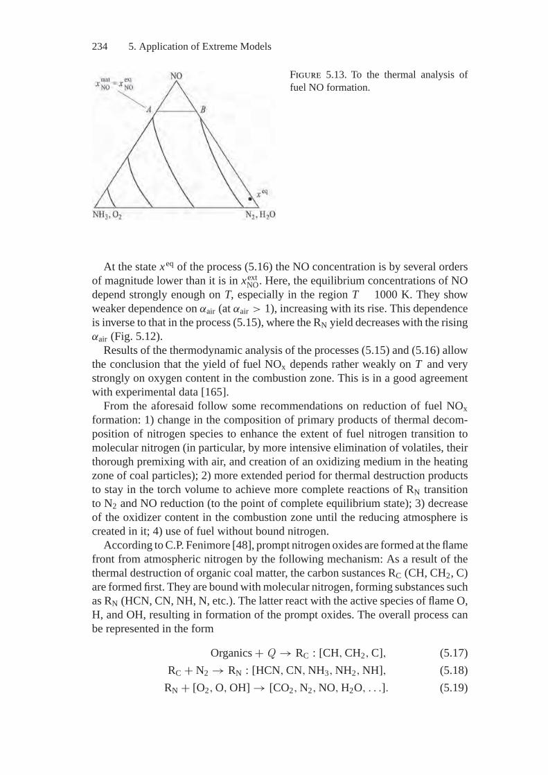
234 5. Application of Extreme Models
Figure 5.13. To the thermal analysis offuel NO formation.
At the state xeq of the process (5.16) the NO concentration is by several ordersof magnitude lower than it is in xext
NO. Here, the equilibrium concentrations of NOdepend strongly enough on T, especially in the region T 1000 K. They showweaker dependence on αair (at αair > 1), increasing with its rise. This dependenceis inverse to that in the process (5.15), where the RN yield decreases with the risingαair (Fig. 5.12).
Results of the thermodynamic analysis of the processes (5.15) and (5.16) allowthe conclusion that the yield of fuel NOx depends rather weakly on T and verystrongly on oxygen content in the combustion zone. This is in a good agreementwith experimental data [165].
From the aforesaid follow some recommendations on reduction of fuel NOxformation: 1) change in the composition of primary products of thermal decom-position of nitrogen species to enhance the extent of fuel nitrogen transition tomolecular nitrogen (in particular, by more intensive elimination of volatiles, theirthorough premixing with air, and creation of an oxidizing medium in the heatingzone of coal particles); 2) more extended period for thermal destruction productsto stay in the torch volume to achieve more complete reactions of RN transitionto N2 and NO reduction (to the point of complete equilibrium state); 3) decreaseof the oxidizer content in the combustion zone until the reducing atmosphere iscreated in it; 4) use of fuel without bound nitrogen.
According to C.P. Fenimore [48], prompt nitrogen oxides are formed at the flamefront from atmospheric nitrogen by the following mechanism: As a result of thethermal destruction of organic coal matter, the carbon sustances RC (CH, CH2, C)are formed first. They are bound with molecular nitrogen, forming substances suchas RN (HCN, CN, NH, N, etc.). The latter react with the active species of flame O,H, and OH, resulting in formation of the prompt oxides. The overall process canbe represented in the form
Organics + Q → RC : [CH, CH2, C], (5.17)RC + N2 → RN : [HCN, CN, NH3, NH2, NH], (5.18)
RN + [O2, O, OH] → [CO2, N2, NO, H2O, . . .]. (5.19)
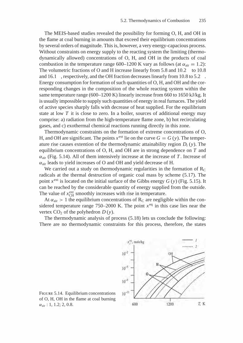
5.2. Thermodynamics of Combustion 235
The MEIS-based studies revealed the possibility for forming O, H, and OH inthe flame at coal burning in amounts that exceed their equilibrium concentrationsby several orders of magnitude. This is, however, a very energy-capacious process.Without constraints on energy supply to the reacting system the limiting (thermo-dynamically allowed) concentrations of O, H, and OH in the products of coalcombustion in the temperature range 600–1200 K vary as follows (at αair = 1.2):The volumetric fractions of O and H increase linearly from 5.8 and 10.2 to 10.8and 16.1 , respectively, and the OH fraction decreases linearly from 10.8 to 5.2 .Energy consumption for formation of such quantities of O, H, and OH and the cor-responding changes in the composition of the whole reacting system within thesame temperature range (600–1200 K) linearly increase from 660 to 1650 kJ/kg. Itis usually impossible to supply such quantities of energy in real furnaces. The yieldof active species sharply falls with decrease of heat supplied. For the equilibriumstate at low T it is close to zero. In a boiler, sources of additional energy maycomprise: a) radiation from the high-temperature flame zone, b) hot recirculatinggases, and c) exothermal chemical reactions running directly in this zone.
Thermodynamic constraints on the formation of extreme concentrations of O,H, and OH are significant. The points xext lie on the curve G = G (y). The temper-ature rise causes extention of the thermodynamic attainability region Dt (y). Theequilibrium concentrations of O, H, and OH are in strong dependence on T andαair (Fig. 5.14). All of them intensively increase at the increase of T . Increase ofαair leads to yield increases of O and OH and yield decrease of H.
We carried out a study on thermodynamic regularities in the formation of RCradicals at the thermal destruction of organic coal mass by scheme (5.17). Thepoint xext is located on the initial surface of the Gibbs energy G (y) (Fig. 5.15). Itcan be reached by the considerable quantity of energy supplied from the outside.The value of xext
CH smoothly increases with rise in temperature.At αair > 1 the equilibrium concentrations of RC are negligible within the con-
sidered temperature range 750–2000 K. The point xeq in this case lies near thevertex CO2 of the polyhedron D (y).
The thermodynamic analysis of process (5.18) lets us conclude the following:There are no thermodynamic constraints for this process, therefore, the states
Figure 5.14. Equilibrium concentrationsof O, H, OH in the flame at coal burningαair : 1, 1.2; 2, 0.8.
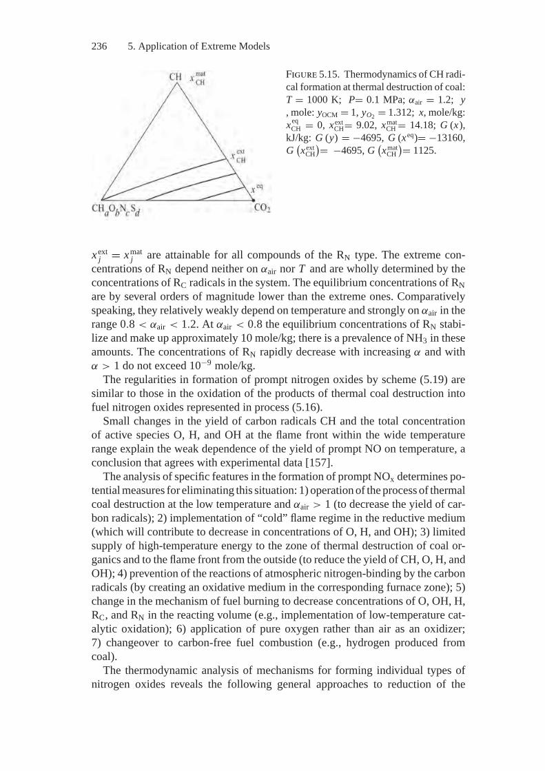
236 5. Application of Extreme Models
Figure 5.15. Thermodynamics of CH radi-cal formation at thermal destruction of coal:T = 1000 K; P= 0.1 MPa; αair = 1.2; y, mole: yOCM = 1, yO2 = 1.312; x, mole/kg:x eq
CH = 0, xextCH= 9.02, xmat
CH = 14.18; G (x),kJ/kg: G (y) = −4695, G (xeq)= −13160,G
(x ext
CH)= −4695, G
(xmat
CH)= 1125.
xextj = xmat
j are attainable for all compounds of the RN type. The extreme con-centrations of RN depend neither on αair nor T and are wholly determined by theconcentrations of RC radicals in the system. The equilibrium concentrations of RNare by several orders of magnitude lower than the extreme ones. Comparativelyspeaking, they relatively weakly depend on temperature and strongly on αair in therange 0.8 < αair < 1.2. At αair < 0.8 the equilibrium concentrations of RN stabi-lize and make up approximately 10 mole/kg; there is a prevalence of NH3 in theseamounts. The concentrations of RN rapidly decrease with increasing α and withα > 1 do not exceed 10−9 mole/kg.
The regularities in formation of prompt nitrogen oxides by scheme (5.19) aresimilar to those in the oxidation of the products of thermal coal destruction intofuel nitrogen oxides represented in process (5.16).
Small changes in the yield of carbon radicals CH and the total concentrationof active species O, H, and OH at the flame front within the wide temperaturerange explain the weak dependence of the yield of prompt NO on temperature, aconclusion that agrees with experimental data [157].
The analysis of specific features in the formation of prompt NOx determines po-tential measures for eliminating this situation: 1) operation of the process of thermalcoal destruction at the low temperature and αair > 1 (to decrease the yield of car-bon radicals); 2) implementation of “cold” flame regime in the reductive medium(which will contribute to decrease in concentrations of O, H, and OH); 3) limitedsupply of high-temperature energy to the zone of thermal destruction of coal or-ganics and to the flame front from the outside (to reduce the yield of CH, O, H, andOH); 4) prevention of the reactions of atmospheric nitrogen-binding by the carbonradicals (by creating an oxidative medium in the corresponding furnace zone); 5)change in the mechanism of fuel burning to decrease concentrations of O, OH, H,RC, and RN in the reacting volume (e.g., implementation of low-temperature cat-alytic oxidation); 6) application of pure oxygen rather than air as an oxidizer;7) changeover to carbon-free fuel combustion (e.g., hydrogen produced fromcoal).
The thermodynamic analysis of mechanisms for forming individual types ofnitrogen oxides reveals the following general approaches to reduction of the
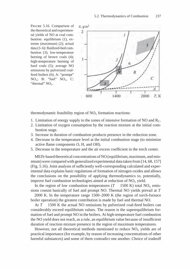
5.2. Thermodynamics of Combustion 237
Figure 5.16. Comparison ofthe theoretical and experimen-tal yields of NO at coal com-bustion: equilibrium (1), ex-treme (maximum) (2); actualdata (3–6): fluidized-bed com-bustion (3); low-temperatureburning of brown coals (4);high-temperature burning ofhard coals (5); average NOemissions by pulverized coal-fired boilers (6); A: “prompt”NOx; B: “fuel” NOx, C:“thermal” NOx.
thermodynamic feasibility region of NOx formation reactions:
1. Limitation of energy supply to the zones of intensive formation of NO and RC.2. Limitation of oxygen consumption by the reaction mixture at the initial com-
bustion stage.3. Increase in duration of combustion products presence in the reduction zone.4. Decrease in the temperature level at the initial combustion stage (to minimize
active flame components O, H, and OH).5. Decrease in the temperature and the air excess coefficient in the torch center.
MEIS-based theoretical concentrations of NO (equilibrium, maximum, and min-imum) were compared with generalized experimental data taken from [14, 68, 157](Fig. 5.16). Joint analysis of sufficiently well-corresponding calculated and exper-imental data explains basic regulations of formation of nitrogen oxides and allowsthe conclusions on the possibility of applying thermodynamics to, potentially,improve fuel combustion technologies aimed at reduction of NOx yield.
In the region of low combustion temperatures (T 1500 K) total NOx emis-sions consist basically of fuel and prompt NO. Thermal NO yields prevail at T
2000 K. In the temperature range 1500–2000 K (the region of torch-furnaceboiler operation) the greatest contribution is made by fuel and thermal NO.
At T 1500 K the actual NO emissions by pulverized coal-fired boilers canconsiderably exceed equilibrium values. The reason is the superequilibrium for-mation of fuel and prompt NO in the boilers. At high-temperature fuel combustionthe NO yield does not reach, as a rule, an equilibrium value because of insufficientduration of reaction mixture presence in the region of maximum temperatures.
However, not all theoretical methods mentioned to reduce NOx yields are ofpractical importance (for example, by reason of increasing concentrations of otherharmful substances) and some of them contradict one another. Choice of tradeoff
238 5. Application of Extreme Models
decisions for specific type of furnaces and kind of fuel involved is an engineer-ing problem whose successful solution may demand additional experimental andkinetic studies. The aim of these studies is to search for and realize on the ther-modynamically attainable set Dt (y) a process trajectory leading to the desirableresult. The theoretical results discussed above may form a basis for this search.
After describing the considered example’s significance in the direct solutionof the problem of NOx suppression in fuel combustion processes, we will takeadvantage of a visualization of the example to demonstrate the “art of the possible”in the thermodynamic analysis of technical systems.
In the given case such an analysis was made based on solely the fragmentarykinetic information on the studied process mechanism: an aggregated descriptionof forming three types of nitrogen oxides. In real systems these processes areinterrelated and in addition to this, their implementation depends on the whole setof reactions running in the system.
The fragmentary character of information was taken into account by applyingthe following scheme of thermodynamic modeling: Idealized models of the leastdimension were used to study independently every parallel branch of the totalmechanism of NOx formation. The study of an individual branch, in turn, wasreduced to the thermodynamic analysis of components of its aggregate stages.The influence of nonideality was evaluated by detailed models including nitrogenoxides and many other harmful compounds.
It is precisely such a stage-by-stage joint application of thermodynamics andkinetics, ideal and detailed “real” models, that allowed the fundamental regularitiesof running the considered processes to be revealed and the potential changes inthe actual characteristics to be evaluated. The most important applied result ofthe analysis performed was the substantiation of measures on control of separatestages.
In our opinion the conclusions drawn proved to be more informative than thosereached by the use of only kinetic models and full-scale experiments with a com-parable scope of studies. The original results of the analysis carried out that wereobtained by its “thermodynamic decomposition” are: 1) explanation of the reasonsfor changing sizes of the thermodynamic attainability region Dt (y) with indicationof possible quantitative relationships between xmat
NO , xextNO, xeq
NO; 2) determination ofthe effect of nonthermodynamic factors (energy and mass exchange, air surplus)on NOx concentrations; 3) appraisal of the possibility to decrease NOx yield be-low the equilibrium values in the case of complete combustion of fuel carbon;4) thermodynamic derivation of a weak temperature dependence of ptompt NOxformation.
Analysis of Environmental Characteristics of Periodic FuelCombustion in Small FurnacesCoal- or wood-fired utility boiler plants and home heating stoves with manual fuelloading are chosen as the object of study. In many cities these small heat sources
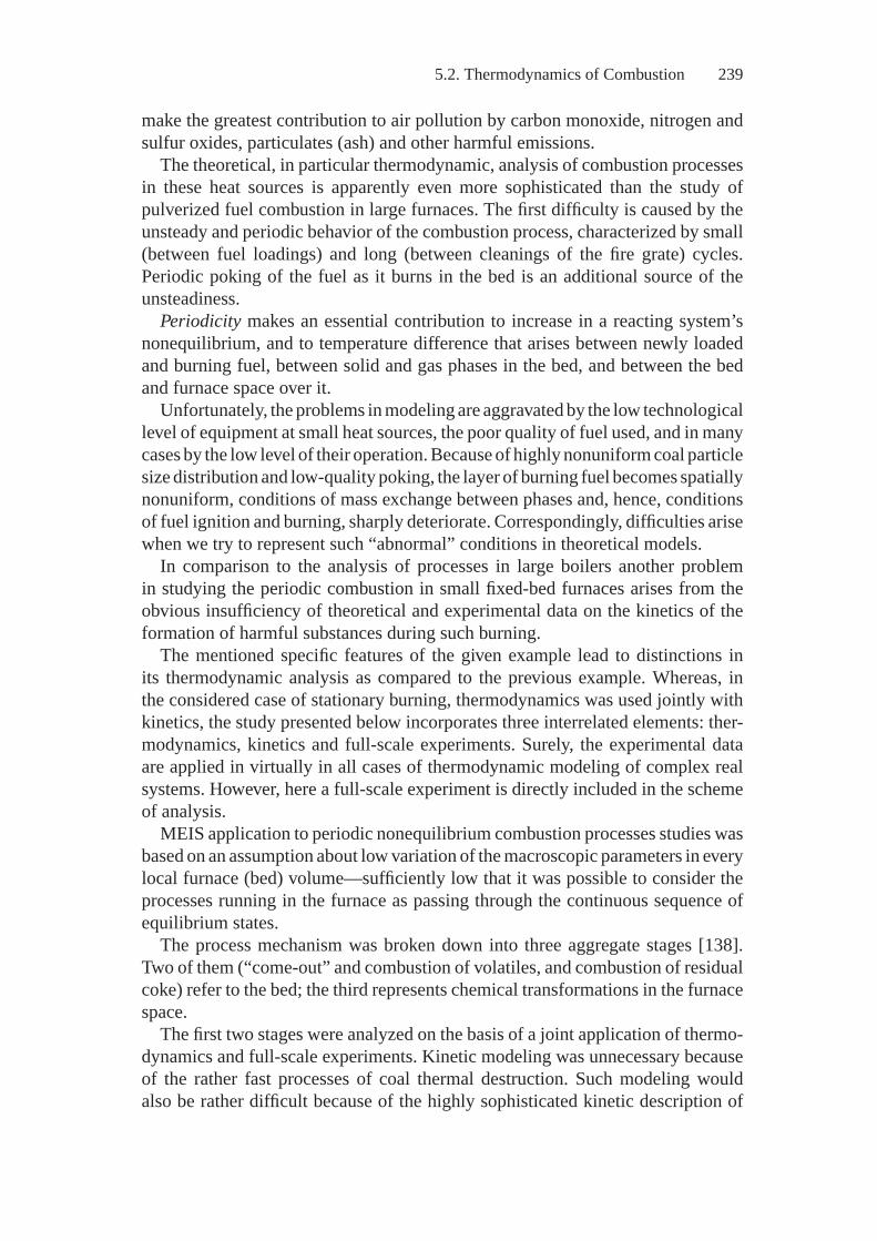
5.2. Thermodynamics of Combustion 239
make the greatest contribution to air pollution by carbon monoxide, nitrogen andsulfur oxides, particulates (ash) and other harmful emissions.
The theoretical, in particular thermodynamic, analysis of combustion processesin these heat sources is apparently even more sophisticated than the study ofpulverized fuel combustion in large furnaces. The first difficulty is caused by theunsteady and periodic behavior of the combustion process, characterized by small(between fuel loadings) and long (between cleanings of the fire grate) cycles.Periodic poking of the fuel as it burns in the bed is an additional source of theunsteadiness.
Periodicity makes an essential contribution to increase in a reacting system’snonequilibrium, and to temperature difference that arises between newly loadedand burning fuel, between solid and gas phases in the bed, and between the bedand furnace space over it.
Unfortunately, the problems in modeling are aggravated by the low technologicallevel of equipment at small heat sources, the poor quality of fuel used, and in manycases by the low level of their operation. Because of highly nonuniform coal particlesize distribution and low-quality poking, the layer of burning fuel becomes spatiallynonuniform, conditions of mass exchange between phases and, hence, conditionsof fuel ignition and burning, sharply deteriorate. Correspondingly, difficulties arisewhen we try to represent such “abnormal” conditions in theoretical models.
In comparison to the analysis of processes in large boilers another problemin studying the periodic combustion in small fixed-bed furnaces arises from theobvious insufficiency of theoretical and experimental data on the kinetics of theformation of harmful substances during such burning.
The mentioned specific features of the given example lead to distinctions inits thermodynamic analysis as compared to the previous example. Whereas, inthe considered case of stationary burning, thermodynamics was used jointly withkinetics, the study presented below incorporates three interrelated elements: ther-modynamics, kinetics and full-scale experiments. Surely, the experimental dataare applied in virtually in all cases of thermodynamic modeling of complex realsystems. However, here a full-scale experiment is directly included in the schemeof analysis.
MEIS application to periodic nonequilibrium combustion processes studies wasbased on an assumption about low variation of the macroscopic parameters in everylocal furnace (bed) volume—sufficiently low that it was possible to consider theprocesses running in the furnace as passing through the continuous sequence ofequilibrium states.
The process mechanism was broken down into three aggregate stages [138].Two of them (“come-out” and combustion of volatiles, and combustion of residualcoke) refer to the bed; the third represents chemical transformations in the furnacespace.
The first two stages were analyzed on the basis of a joint application of thermo-dynamics and full-scale experiments. Kinetic modeling was unnecessary becauseof the rather fast processes of coal thermal destruction. Such modeling wouldalso be rather difficult because of the highly sophisticated kinetic description of
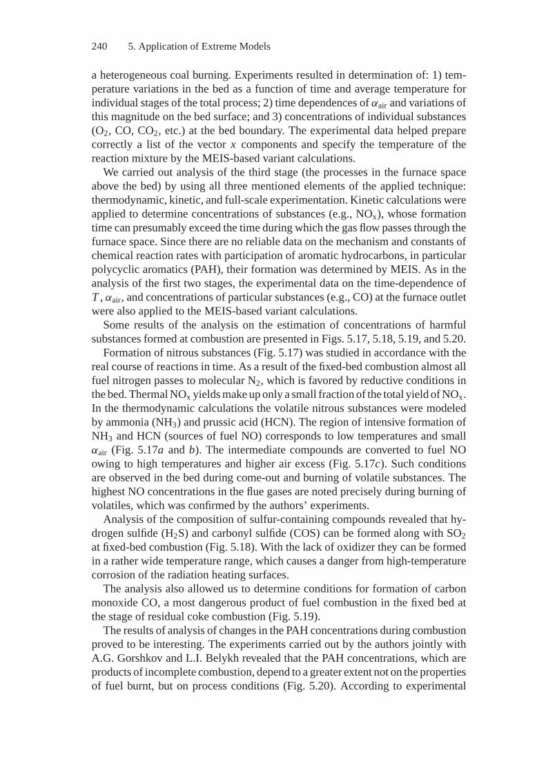
240 5. Application of Extreme Models
a heterogeneous coal burning. Experiments resulted in determination of: 1) tem-perature variations in the bed as a function of time and average temperature forindividual stages of the total process; 2) time dependences of αair and variations ofthis magnitude on the bed surface; and 3) concentrations of individual substances(O2, CO, CO2, etc.) at the bed boundary. The experimental data helped preparecorrectly a list of the vector x components and specify the temperature of thereaction mixture by the MEIS-based variant calculations.
We carried out analysis of the third stage (the processes in the furnace spaceabove the bed) by using all three mentioned elements of the applied technique:thermodynamic, kinetic, and full-scale experimentation. Kinetic calculations wereapplied to determine concentrations of substances (e.g., NOx), whose formationtime can presumably exceed the time during which the gas flow passes through thefurnace space. Since there are no reliable data on the mechanism and constants ofchemical reaction rates with participation of aromatic hydrocarbons, in particularpolycyclic aromatics (PAH), their formation was determined by MEIS. As in theanalysis of the first two stages, the experimental data on the time-dependence ofT , αair, and concentrations of particular substances (e.g., CO) at the furnace outletwere also applied to the MEIS-based variant calculations.
Some results of the analysis on the estimation of concentrations of harmfulsubstances formed at combustion are presented in Figs. 5.17, 5.18, 5.19, and 5.20.
Formation of nitrous substances (Fig. 5.17) was studied in accordance with thereal course of reactions in time. As a result of the fixed-bed combustion almost allfuel nitrogen passes to molecular N2, which is favored by reductive conditions inthe bed. Thermal NOx yields make up only a small fraction of the total yield of NOx.In the thermodynamic calculations the volatile nitrous substances were modeledby ammonia (NH3) and prussic acid (HCN). The region of intensive formation ofNH3 and HCN (sources of fuel NO) corresponds to low temperatures and smallαair (Fig. 5.17a and b). The intermediate compounds are converted to fuel NOowing to high temperatures and higher air excess (Fig. 5.17c). Such conditionsare observed in the bed during come-out and burning of volatile substances. Thehighest NO concentrations in the flue gases are noted precisely during burning ofvolatiles, which was confirmed by the authors’ experiments.
Analysis of the composition of sulfur-containing compounds revealed that hy-drogen sulfide (H2S) and carbonyl sulfide (COS) can be formed along with SO2at fixed-bed combustion (Fig. 5.18). With the lack of oxidizer they can be formedin a rather wide temperature range, which causes a danger from high-temperaturecorrosion of the radiation heating surfaces.
The analysis also allowed us to determine conditions for formation of carbonmonoxide CO, a most dangerous product of fuel combustion in the fixed bed atthe stage of residual coke combustion (Fig. 5.19).
The results of analysis of changes in the PAH concentrations during combustionproved to be interesting. The experiments carried out by the authors jointly withA.G. Gorshkov and L.I. Belykh revealed that the PAH concentrations, which areproducts of incomplete combustion, depend to a greater extent not on the propertiesof fuel burnt, but on process conditions (Fig. 5.20). According to experimental
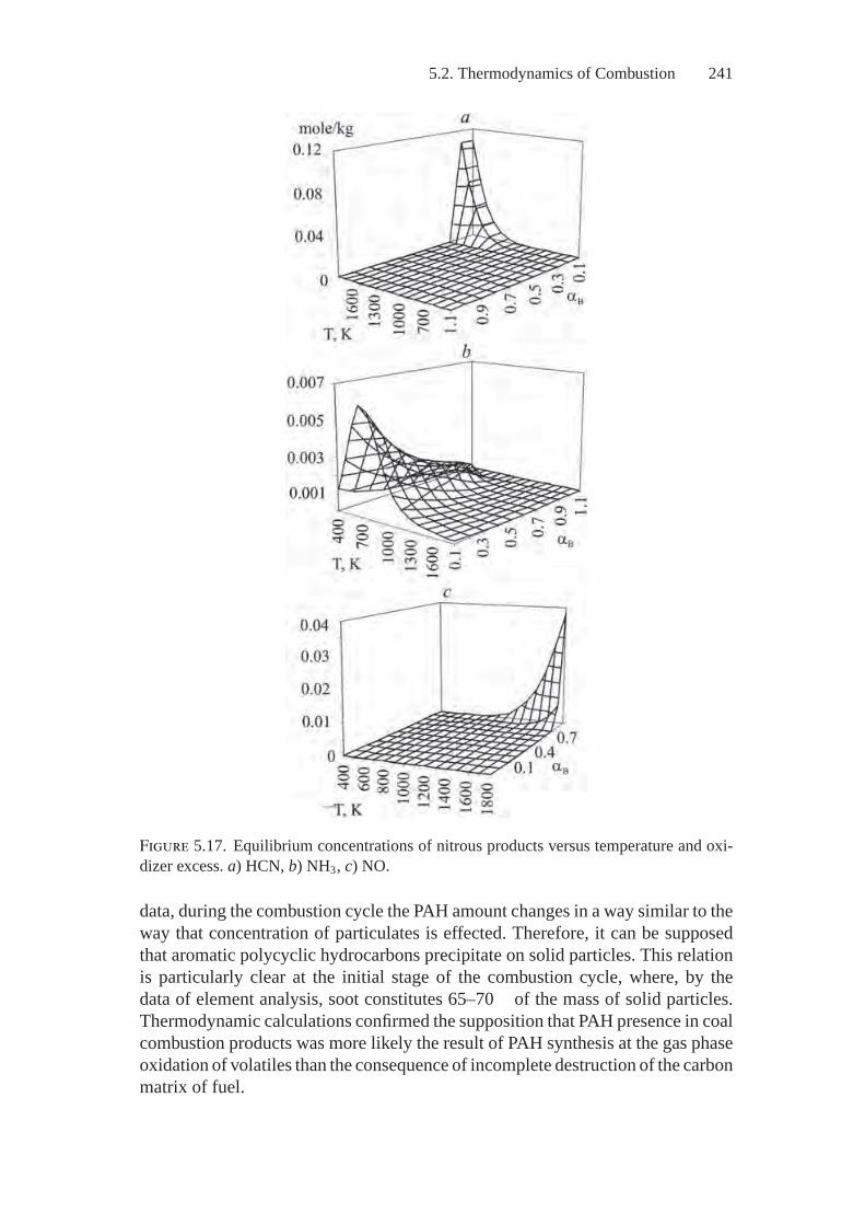
5.2. Thermodynamics of Combustion 241
Figure 5.17. Equilibrium concentrations of nitrous products versus temperature and oxi-dizer excess. a) HCN, b) NH3, c) NO.
data, during the combustion cycle the PAH amount changes in a way similar to theway that concentration of particulates is effected. Therefore, it can be supposedthat aromatic polycyclic hydrocarbons precipitate on solid particles. This relationis particularly clear at the initial stage of the combustion cycle, where, by thedata of element analysis, soot constitutes 65–70 of the mass of solid particles.Thermodynamic calculations confirmed the supposition that PAH presence in coalcombustion products was more likely the result of PAH synthesis at the gas phaseoxidation of volatiles than the consequence of incomplete destruction of the carbonmatrix of fuel.
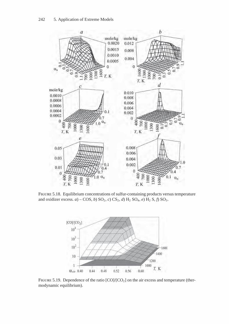
242 5. Application of Extreme Models
Figure 5.18. Equilibrium concentrations of sulfur-containing products versus temperatureand oxidizer excess. a) – COS, b) SO2, c) CS2, d) H2 SO4, e) H2 S, f) SO3.
Figure 5.19. Dependence of the ratio [CO]/[CO2] on the air excess and temperature (ther-modynamic equilibrium).
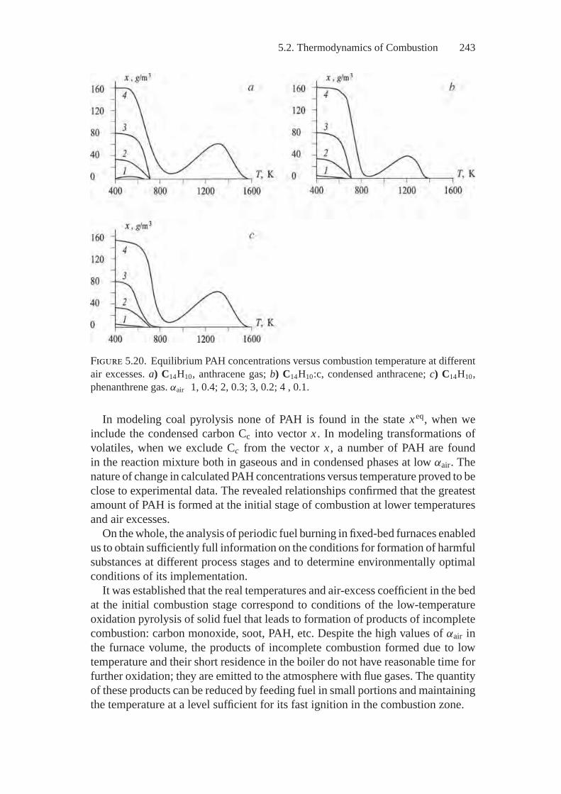
5.2. Thermodynamics of Combustion 243
Figure 5.20. Equilibrium PAH concentrations versus combustion temperature at differentair excesses. a) C14H10, anthracene gas; b) C14H10:c, condensed anthracene; c) C14H10,phenanthrene gas. αair 1, 0.4; 2, 0.3; 3, 0.2; 4 , 0.1.
In modeling coal pyrolysis none of PAH is found in the state xeq, when weinclude the condensed carbon Cc into vector x . In modeling transformations ofvolatiles, when we exclude Cc from the vector x , a number of PAH are foundin the reaction mixture both in gaseous and in condensed phases at low αair. Thenature of change in calculated PAH concentrations versus temperature proved to beclose to experimental data. The revealed relationships confirmed that the greatestamount of PAH is formed at the initial stage of combustion at lower temperaturesand air excesses.
On the whole, the analysis of periodic fuel burning in fixed-bed furnaces enabledus to obtain sufficiently full information on the conditions for formation of harmfulsubstances at different process stages and to determine environmentally optimalconditions of its implementation.
It was established that the real temperatures and air-excess coefficient in the bedat the initial combustion stage correspond to conditions of the low-temperatureoxidation pyrolysis of solid fuel that leads to formation of products of incompletecombustion: carbon monoxide, soot, PAH, etc. Despite the high values of αair inthe furnace volume, the products of incomplete combustion formed due to lowtemperature and their short residence in the boiler do not have reasonable time forfurther oxidation; they are emitted to the atmosphere with flue gases. The quantityof these products can be reduced by feeding fuel in small portions and maintainingthe temperature at a level sufficient for its fast ignition in the combustion zone.
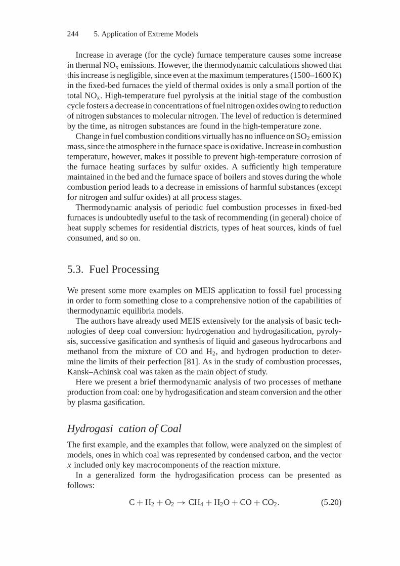
244 5. Application of Extreme Models
Increase in average (for the cycle) furnace temperature causes some increasein thermal NOx emissions. However, the thermodynamic calculations showed thatthis increase is negligible, since even at the maximum temperatures (1500–1600 K)in the fixed-bed furnaces the yield of thermal oxides is only a small portion of thetotal NOx. High-temperature fuel pyrolysis at the initial stage of the combustioncycle fosters a decrease in concentrations of fuel nitrogen oxides owing to reductionof nitrogen substances to molecular nitrogen. The level of reduction is determinedby the time, as nitrogen substances are found in the high-temperature zone.
Change in fuel combustion conditions virtually has no influence on SO2 emissionmass, since the atmosphere in the furnace space is oxidative. Increase in combustiontemperature, however, makes it possible to prevent high-temperature corrosion ofthe furnace heating surfaces by sulfur oxides. A sufficiently high temperaturemaintained in the bed and the furnace space of boilers and stoves during the wholecombustion period leads to a decrease in emissions of harmful substances (exceptfor nitrogen and sulfur oxides) at all process stages.
Thermodynamic analysis of periodic fuel combustion processes in fixed-bedfurnaces is undoubtedly useful to the task of recommending (in general) choice ofheat supply schemes for residential districts, types of heat sources, kinds of fuelconsumed, and so on.
5.3. Fuel Processing
We present some more examples on MEIS application to fossil fuel processingin order to form something close to a comprehensive notion of the capabilities ofthermodynamic equilibria models.
The authors have already used MEIS extensively for the analysis of basic tech-nologies of deep coal conversion: hydrogenation and hydrogasification, pyroly-sis, successive gasification and synthesis of liquid and gaseous hydrocarbons andmethanol from the mixture of CO and H2, and hydrogen production to deter-mine the limits of their perfection [81]. As in the study of combustion processes,Kansk–Achinsk coal was taken as the main object of study.
Here we present a brief thermodynamic analysis of two processes of methaneproduction from coal: one by hydrogasification and steam conversion and the otherby plasma gasification.
Hydrogasi cation of CoalThe first example, and the examples that follow, were analyzed on the simplest ofmodels, ones in which coal was represented by condensed carbon, and the vectorx included only key macrocomponents of the reaction mixture.
In a generalized form the hydrogasification process can be presented asfollows:
C + H2 + O2 → CH4 + H2O + CO + CO2. (5.20)
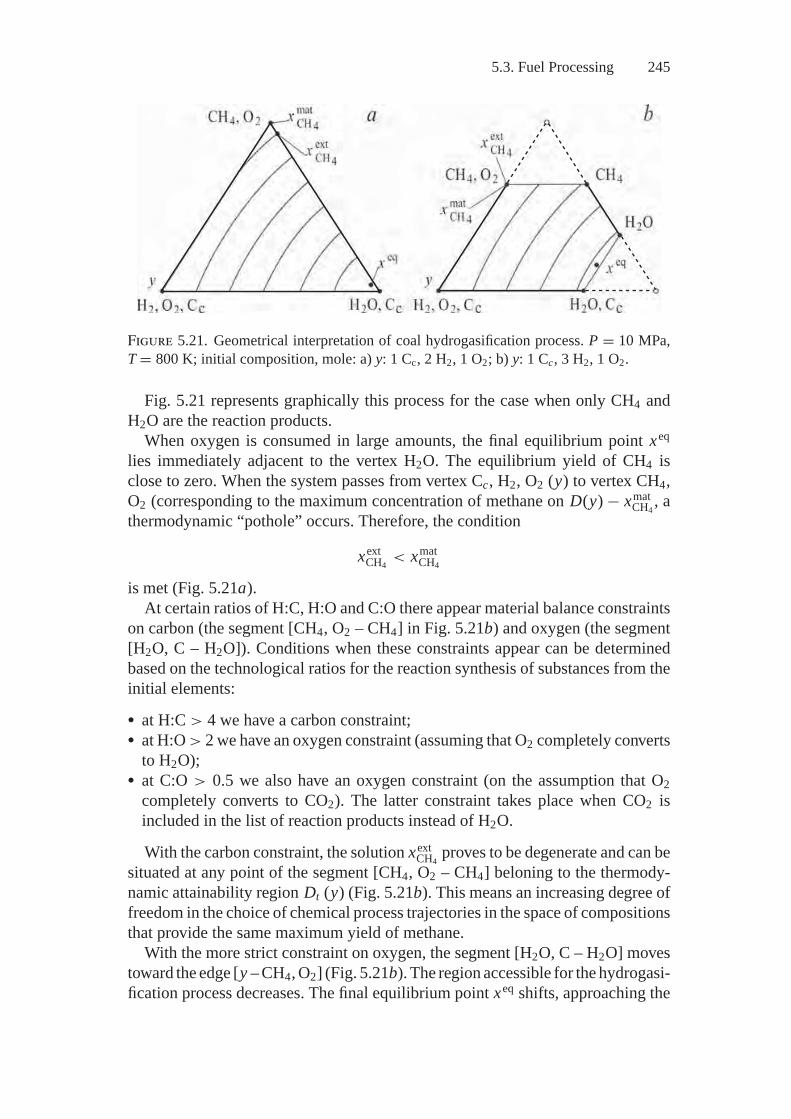
5.3. Fuel Processing 245
Figure 5.21. Geometrical interpretation of coal hydrogasification process. P = 10 MPa,T = 800 K; initial composition, mole: a) y: 1 Cc, 2 H2, 1 O2; b) y: 1 Cc, 3 H2, 1 O2.
Fig. 5.21 represents graphically this process for the case when only CH4 andH2O are the reaction products.
When oxygen is consumed in large amounts, the final equilibrium point xeq
lies immediately adjacent to the vertex H2O. The equilibrium yield of CH4 isclose to zero. When the system passes from vertex Cc, H2, O2 (y) to vertex CH4,O2 (corresponding to the maximum concentration of methane on D(y) − xmat
CH4, a
thermodynamic “pothole” occurs. Therefore, the condition
xextCH4
< xmatCH4
is met (Fig. 5.21a).At certain ratios of H:C, H:O and C:O there appear material balance constraints
on carbon (the segment [CH4, O2 – CH4] in Fig. 5.21b) and oxygen (the segment[H2O, C – H2O]). Conditions when these constraints appear can be determinedbased on the technological ratios for the reaction synthesis of substances from theinitial elements:� at H:C > 4 we have a carbon constraint;� at H:O > 2 we have an oxygen constraint (assuming that O2 completely converts
to H2O);� at C:O > 0.5 we also have an oxygen constraint (on the assumption that O2
completely converts to CO2). The latter constraint takes place when CO2 isincluded in the list of reaction products instead of H2O.
With the carbon constraint, the solution xextCH4
proves to be degenerate and can besituated at any point of the segment [CH4, O2 – CH4] beloning to the thermody-namic attainability region Dt (y) (Fig. 5.21b). This means an increasing degree offreedom in the choice of chemical process trajectories in the space of compositionsthat provide the same maximum yield of methane.
With the more strict constraint on oxygen, the segment [H2O, C – H2O] movestoward the edge [y – CH4, O2] (Fig. 5.21b). The region accessible for the hydrogasi-fication process decreases. The final equilibrium point xeq shifts, approaching the
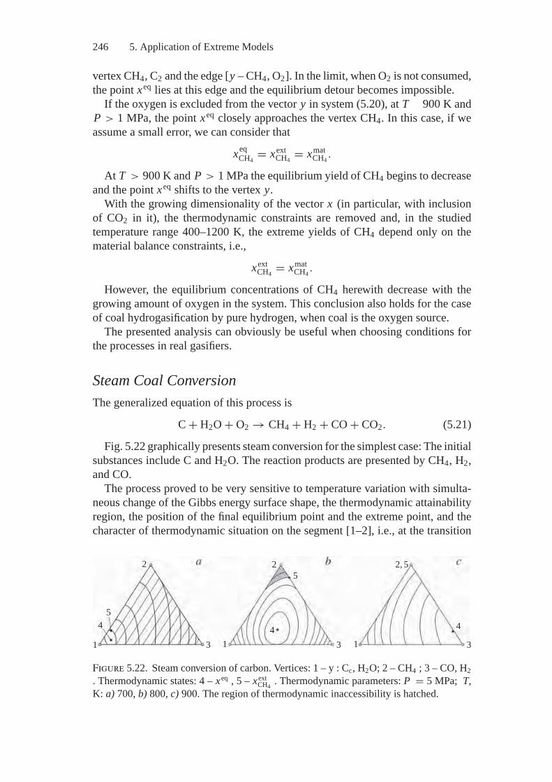
246 5. Application of Extreme Models
vertex CH4, C2 and the edge [y – CH4, O2]. In the limit, when O2 is not consumed,the point xeq lies at this edge and the equilibrium detour becomes impossible.
If the oxygen is excluded from the vector y in system (5.20), at T 900 K andP > 1 MPa, the point xeq closely approaches the vertex CH4. In this case, if weassume a small error, we can consider that
xeqCH4
= xextCH4
= xmatCH4
.
At T > 900 K and P > 1 MPa the equilibrium yield of CH4 begins to decreaseand the point xeq shifts to the vertex y.
With the growing dimensionality of the vector x (in particular, with inclusionof CO2 in it), the thermodynamic constraints are removed and, in the studiedtemperature range 400–1200 K, the extreme yields of CH4 depend only on thematerial balance constraints, i.e.,
xextCH4
= xmatCH4
.
However, the equilibrium concentrations of CH4 herewith decrease with thegrowing amount of oxygen in the system. This conclusion also holds for the caseof coal hydrogasification by pure hydrogen, when coal is the oxygen source.
The presented analysis can obviously be useful when choosing conditions forthe processes in real gasifiers.
Steam Coal ConversionThe generalized equation of this process is
C + H2O + O2 → CH4 + H2 + CO + CO2. (5.21)
Fig. 5.22 graphically presents steam conversion for the simplest case: The initialsubstances include C and H2O. The reaction products are presented by CH4, H2,and CO.
The process proved to be very sensitive to temperature variation with simulta-neous change of the Gibbs energy surface shape, the thermodynamic attainabilityregion, the position of the final equilibrium point and the extreme point, and thecharacter of thermodynamic situation on the segment [1–2], i.e., at the transition
2 2 2, 5
5
5
4
3 1 13 3
4 4
1
Figure 5.22. Steam conversion of carbon. Vertices: 1 – y : Cc, H2O; 2 – CH4 ; 3 – CO, H2. Thermodynamic states: 4 – xeq , 5 – xext
CH4 . Thermodynamic parameters: P = 5 MPa; T,K: a) 700, b) 800, c) 900. The region of thermodynamic inaccessibility is hatched.
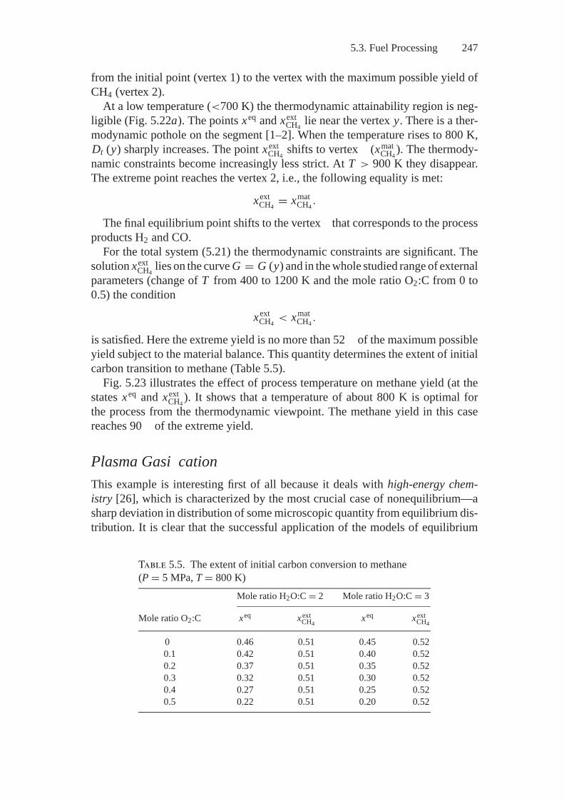
5.3. Fuel Processing 247
from the initial point (vertex 1) to the vertex with the maximum possible yield ofCH4 (vertex 2).
At a low temperature (<700 K) the thermodynamic attainability region is neg-ligible (Fig. 5.22a). The points xeq and xext
CH4lie near the vertex y. There is a ther-
modynamic pothole on the segment [1–2]. When the temperature rises to 800 K,Dt (y) sharply increases. The point xext
CH4shifts to vertex (xmat
CH4). The thermody-
namic constraints become increasingly less strict. At T > 900 K they disappear.The extreme point reaches the vertex 2, i.e., the following equality is met:
xextCH4
= xmatCH4
.
The final equilibrium point shifts to the vertex that corresponds to the processproducts H2 and CO.
For the total system (5.21) the thermodynamic constraints are significant. Thesolution xext
CH4lies on the curve G = G (y) and in the whole studied range of external
parameters (change of T from 400 to 1200 K and the mole ratio O2:C from 0 to0.5) the condition
xextCH4
< xmatCH4
.
is satisfied. Here the extreme yield is no more than 52 of the maximum possibleyield subject to the material balance. This quantity determines the extent of initialcarbon transition to methane (Table 5.5).
Fig. 5.23 illustrates the effect of process temperature on methane yield (at thestates xeq and xext
CH4). It shows that a temperature of about 800 K is optimal for
the process from the thermodynamic viewpoint. The methane yield in this casereaches 90 of the extreme yield.
Plasma Gasi cationThis example is interesting first of all because it deals with high-energy chem-istry [26], which is characterized by the most crucial case of nonequilibrium—asharp deviation in distribution of some microscopic quantity from equilibrium dis-tribution. It is clear that the successful application of the models of equilibrium
Table 5.5. The extent of initial carbon conversion to methane(P = 5 MPa, T = 800 K)
Mole ratio H2O:C = 2 Mole ratio H2O:C = 3
Mole ratio O2:C xeq xextCH4
xeq xextCH4
0 0.46 0.51 0.45 0.520.1 0.42 0.51 0.40 0.520.2 0.37 0.51 0.35 0.520.3 0.32 0.51 0.30 0.520.4 0.27 0.51 0.25 0.520.5 0.22 0.51 0.20 0.52
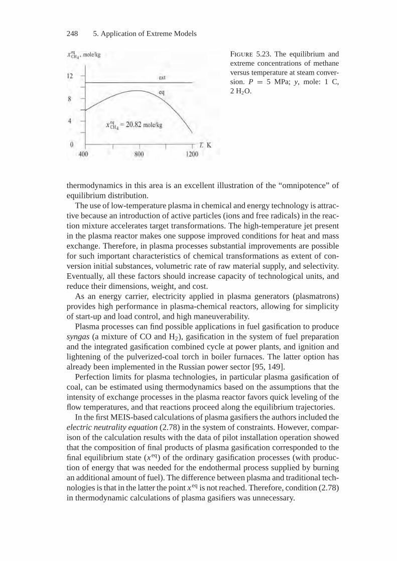
248 5. Application of Extreme Models
Figure 5.23. The equilibrium andextreme concentrations of methaneversus temperature at steam conver-sion. P = 5 MPa; y, mole: 1 C,2 H2O.
thermodynamics in this area is an excellent illustration of the “omnipotence” ofequilibrium distribution.
The use of low-temperature plasma in chemical and energy technology is attrac-tive because an introduction of active particles (ions and free radicals) in the reac-tion mixture accelerates target transformations. The high-temperature jet presentin the plasma reactor makes one suppose improved conditions for heat and massexchange. Therefore, in plasma processes substantial improvements are possiblefor such important characteristics of chemical transformations as extent of con-version initial substances, volumetric rate of raw material supply, and selectivity.Eventually, all these factors should increase capacity of technological units, andreduce their dimensions, weight, and cost.
As an energy carrier, electricity applied in plasma generators (plasmatrons)provides high performance in plasma-chemical reactors, allowing for simplicityof start-up and load control, and high maneuverability.
Plasma processes can find possible applications in fuel gasification to producesyngas (a mixture of CO and H2), gasification in the system of fuel preparationand the integrated gasification combined cycle at power plants, and ignition andlightening of the pulverized-coal torch in boiler furnaces. The latter option hasalready been implemented in the Russian power sector [95, 149].
Perfection limits for plasma technologies, in particular plasma gasification ofcoal, can be estimated using thermodynamics based on the assumptions that theintensity of exchange processes in the plasma reactor favors quick leveling of theflow temperatures, and that reactions proceed along the equilibrium trajectories.
In the first MEIS-based calculations of plasma gasifiers the authors included theelectric neutrality equation (2.78) in the system of constraints. However, compar-ison of the calculation results with the data of pilot installation operation showedthat the composition of final products of plasma gasification corresponded to thefinal equilibrium state (xeq) of the ordinary gasification processes (with produc-tion of energy that was needed for the endothermal process supplied by burningan additional amount of fuel). The difference between plasma and traditional tech-nologies is that in the latter the point xeq is not reached. Therefore, condition (2.78)in thermodynamic calculations of plasma gasifiers was unnecessary.
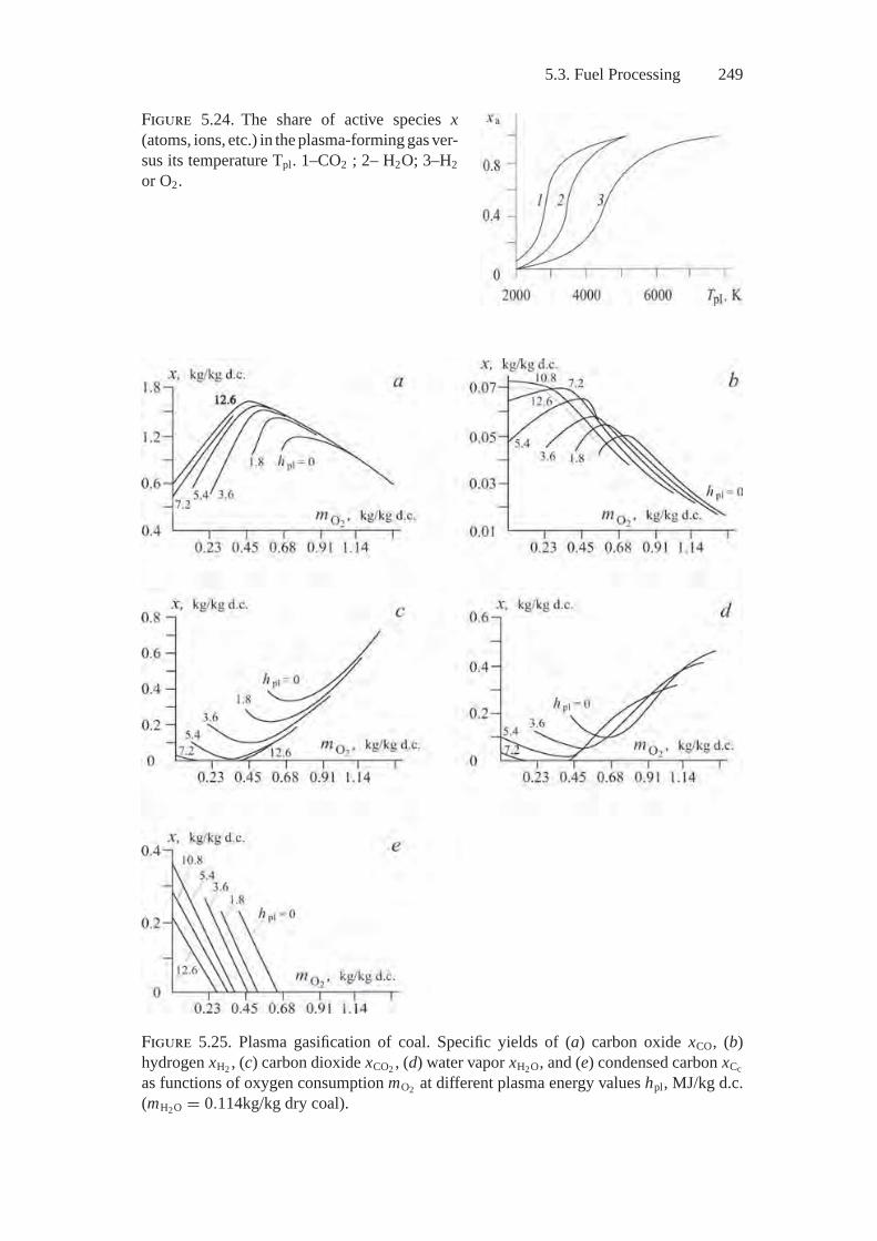
5.3. Fuel Processing 249
Figure 5.24. The share of active species x(atoms, ions, etc.) in the plasma-forming gas ver-sus its temperature Tpl. 1–CO2 ; 2– H2O; 3–H2or O2.
Figure 5.25. Plasma gasification of coal. Specific yields of (a) carbon oxide xCO, (b)hydrogen xH2 , (c) carbon dioxide xCO2 , (d) water vapor xH2O, and (e) condensed carbon xCcas functions of oxygen consumption mO2 at different plasma energy values hpl, MJ/kg d.c.(mH2O = 0.114kg/kg dry coal).
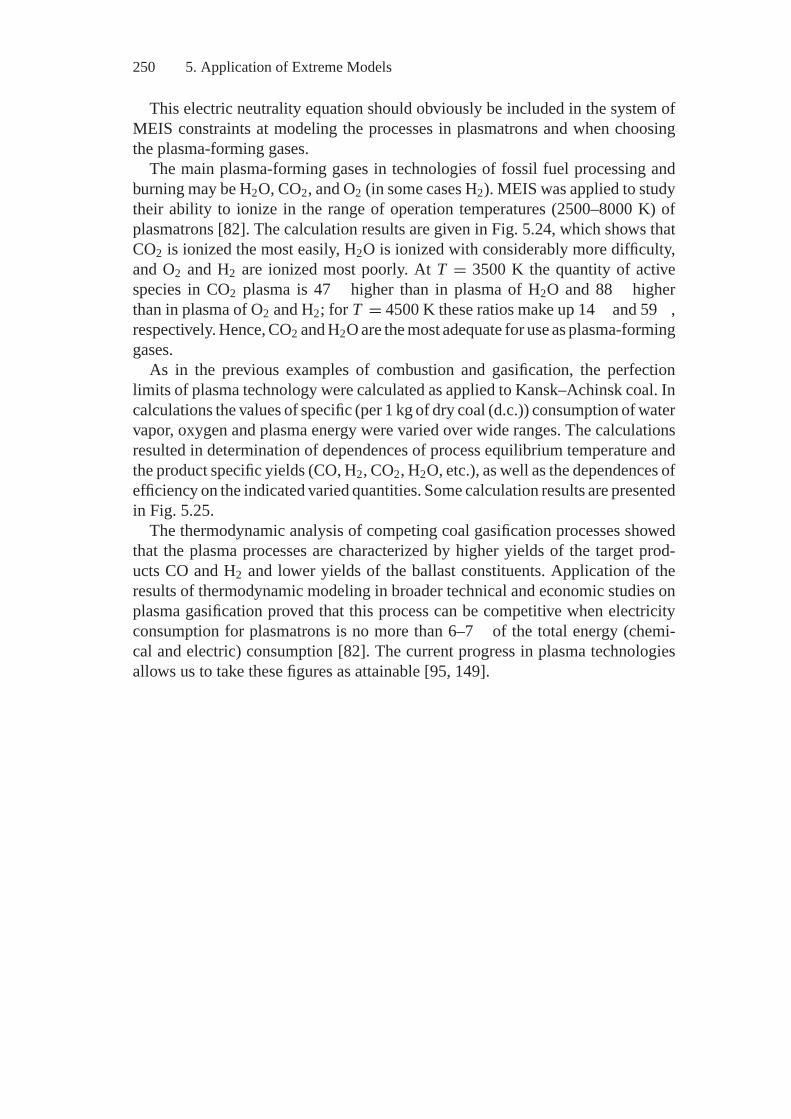
250 5. Application of Extreme Models
This electric neutrality equation should obviously be included in the system ofMEIS constraints at modeling the processes in plasmatrons and when choosingthe plasma-forming gases.
The main plasma-forming gases in technologies of fossil fuel processing andburning may be H2O, CO2, and O2 (in some cases H2). MEIS was applied to studytheir ability to ionize in the range of operation temperatures (2500–8000 K) ofplasmatrons [82]. The calculation results are given in Fig. 5.24, which shows thatCO2 is ionized the most easily, H2O is ionized with considerably more difficulty,and O2 and H2 are ionized most poorly. At T = 3500 K the quantity of activespecies in CO2 plasma is 47 higher than in plasma of H2O and 88 higherthan in plasma of O2 and H2; for T = 4500 K these ratios make up 14 and 59 ,respectively. Hence, CO2 and H2O are the most adequate for use as plasma-forminggases.
As in the previous examples of combustion and gasification, the perfectionlimits of plasma technology were calculated as applied to Kansk–Achinsk coal. Incalculations the values of specific (per 1 kg of dry coal (d.c.)) consumption of watervapor, oxygen and plasma energy were varied over wide ranges. The calculationsresulted in determination of dependences of process equilibrium temperature andthe product specific yields (CO, H2, CO2, H2O, etc.), as well as the dependences ofefficiency on the indicated varied quantities. Some calculation results are presentedin Fig. 5.25.
The thermodynamic analysis of competing coal gasification processes showedthat the plasma processes are characterized by higher yields of the target prod-ucts CO and H2 and lower yields of the ballast constituents. Application of theresults of thermodynamic modeling in broader technical and economic studies onplasma gasification proved that this process can be competitive when electricityconsumption for plasmatrons is no more than 6–7 of the total energy (chemi-cal and electric) consumption [82]. The current progress in plasma technologiesallows us to take these figures as attainable [95, 149].
Conclusion
We never know a response to our word.F. . Tyutchev
What makes us, the authors, look to further fruitful development of the scientificsubject whose basic concepts we tried to present in the book Replying to thisquestion, we can mention several encouraging factors.
First of all, we are optimistic, because the created thermodynamic models havealready been used to solve successfully a rather wide scope of theoretical andapplied problems. They are: determination of maximum possible yields of thetarget products in fossil fuel conversion technologies; assessment of environmen-tal characteristics of continuous and periodic combustion processes; analysis ofharmful substance behavior in the atmosphere; and calculation of flow distributionin multiloop hydraulic systems.
An even greater number of unsolved problems including those manifested them-selves in the analysis of the solved problems tell us that we have correctly chosenthis specific area of studies. By Hilbert [69], “Any scientific sphere is viable, aslong as there is an excess of new problems in it. The lack of new problems meansdying off or termination of independent development.” From the text of the bookfollow some problem statements for future studies. Some examples are creationof strictly formalized methods based on the idea of a thermodynamic tree, con-struction of the thermodynamic model of an atmospheric aerosol, and descriptionof a sufficiently complete system of kinetic constraints in equilibrium models ofcombustion and atmospheric pollution processes.
In our opinion the book allows a deeper understanding of the logic of thermo-dynamics development, the link between the present-day models and the initialideas of its founders. Whereas the principles of inertia, relativity, and equilib-rium established by Galilei clarified the possibility to replace description of theuniform straight-line motion by the model of rest, the thermodynamic works byBoltzmann and Gibbs revealed the possibility of describing processes in systemsconsisting of a colossal number of elements and subject to statistical laws in equi-librium terms. Such systems in fact take in all the macroscopic systems interactingwith the environment at fixed parameters in which the processes of substance and
251

252 Conclusion
energy conversion take place. MEIS application enabled the use of potentialitiesof thermodynamics (that were understood yet by Boltzmann and Gibbs) to analyzeany admissible states (complete and partial equilibria) of equilibrium systems andthe search for thermodynamic attainability regions in these systems. Interrelationsbetween models of motion (those including the time variable) and models of states,as well as areas of admissible and expedient application of these models to solvediverse physicochemical and technical problems are features that became moreclear to us as researchers.
The noted circumstances make us hope that, in parallel with development ofsuch acknowledged current scientific disciplines as synergetics and nonequilibriumthermodynamics, classical equilibrium thermodynamics will enter into a new stageof advancement.
There is also much doubt about such further favorable and desirable (for theauthors) courses of events. This is not just because the “old” sciences are notfancy and attractive for young researchers; more to the point, if new models basedon old theories are to become accessible to a wide circle of specialists and tofind application in many research and design works, the appropriate software andcommercial computing systems will have to be created. This requires great effort ofentire teams because every new field of MEIS application calls for modification ofthe key algorithms, replenishment or creation of new data banks (primarily on thethermodynamic properties of substances), and design of special auxiliary softwareregarding the objectives of the study. The authors can only partially solve theproblems that arise. In the immediate future we plan both to solve some theoreticaland methodological problems (such as construction of the thermodynamic tree onpartial graphs) and to create an effective heavy duty software for detailed analysisof particular applied problems, such as formation of harmful substances in torchand fixed-bed furnaces, description of processes on the surface of aerosols in theatmosphere, and air exchange in buildings and structures in normal and emergency(at fires) conditions.
Afterword
So far MEIS applications have been associated to a great extent with the regrettableconsequences of human activity, adverse impacts on the environment we inhabit.We would prefer to be engaged in more pleasant calculations, for example, onthe calculation of the extent to which nature eventually recovers from damage,a recovery owing to the skillful tending by human beings. Well, such a brightfuture could be imagined allowing that these calculations be necessary. “We neverknow. . . .”
SupplementThe Model of Extreme Intermediate States (MEIS) andDescription of Nonequilibrium Irreversible Processes
Die Energie der Welt ist Constant.Die Entropie der Welt strebt einem Maximum zu.
R. Clausius
ntroductory RemarksDuring the four years after the publication of the Russian edition of this book, stud-ies on attainability regions and partial equilibria took place in the areas consideredin the book and in new areas of MEIS applications.
The new practical problems solved on the basis of MEIS included: modelingof heating surface slugging in boiler furnaces [153]; estimation of environmentalcharacteristics of combustion chambers in gas turbines [87, 89]; calculation of low-grade fuel gasification processes [103]; analysis of condensation nuclei formationin the atmosphere [90]; and others.
The mathematical features of MEIS being analyzed include, among others:possibilities of solution degeneracy in the search for points xmat and xext
c ; casesof incompatible systems of constraints that determine Dt (y); and dependence oftotal Gibbs energy of the atmospheric system on the radii of the aerosols formedin it. The problem of MEIS reducibility to the convex programming (CP) prob-lems remains the main problem in the mathematical studies. We are now lookingfor convex approximations of the problems for the cases when: the sought vari-ables include the radii of nuclei of the forming phases; the modeled system hasDebey–Huckel solutions, and so on. The analysis of mathematical features, inturn, becomes the basis for correction and improvement of the computationalalgorithms.
Currently, the development of a commercial computational system is nearingcompletion. This system is intended for thermodynamic analysis of technologicaland natural processes [87] and may be applied to the problems of:
� estimating maximum energy and resource efficiency (efficiency, specific fuelconsumption, specific yield of target products and by-products) of differentindustrial technologies;
253
254 Supplement
� revealing the energy-saving potential in production of energy and chemicals, oilrefining, metallurgy and other industries
� determining the assortment and maximum emissions of harmful substances bytechnological plants under normal and emergency operation conditions
� studying the transformations of anthropogenic emissions in the atmosphere, soiland water reservoirs.
The main direction of MEIS development is now formulation of MEIS-basedthermodynamic descriptions (those eliminating the time variable) of chemicalkinetics and transfer process. This work was encouraged, first of all, by the need toassess the practical feasibility of the calculated xext determined by reaction ratesand transfer of mass, energy, impulse, and charges. The problems of equilibriumfeasibility were considered briefly in Section 4.5. There we presented examples ofthe impact of chemical reaction rates on the feasibility of states xext.
Additionally, the equilibrium description of “motions,” which is the subject ofstudies in nonequilibrium thermodynamics and synergetics, is important from theviewpoint of determining MEIS significance in modern scientific areas related toclassical thermodynamics. It is quite clear that for this new scientific concept tobecome the handy tool for researchers and engineers, it is necessary not only togive it a strictly formalized description and theoretical and experimental groundsbut to compare it with competing approaches in the area where it is applied.
Some results obtained from the analysis of MEIS containing description ofmotions and its efficiency are presented below.
On the Possibility to Describe Motions in Termsof Equilibrium ThermodynamicsThe body of the book has already given the examples of “equilibrium” deriva-tions of equations for nonequilibrium irreversible processes: diffusion, heat trans-fer, hydraulic shock, etc. In the Introduction (Section I.2) consideration wasgiven to the applicability of the equilibrium principle to description of the sys-tems that may have various effects (including self-oscillations and spatial or-dering) during their relaxation towards equilibrium. Chapter 5 shows the MEISapplicability for the analysis of high-energy chemical processes (on the exam-ple of plasma coal gasification) and periodic solid fuel combustion processes. Inthe latter case the MEIS was applied along with kinetic models and full-scaleexperiments.
However, the potentialities of equilibrium thermodynamics in studying“motions” may most completely be revealed by analyzing the single model thatcontains both a description of a monotonically changing characteristic function ofthe system at issue and a description of the processes that limit the region of thischange. Before discussing such a model let us make some remarks on the historyof the equilibrium descriptions of motion. Unlike the excursus on the history thatwas made in Sections 1.1 and 1.2 here we will try to focus on the principles thatwill be directly used when developing new MEIS versions.
Supplement 255
Originally, equilibrium models were developed within classical mechanics(Galilei, Euler, D’Alembert, Lagrange, Hamilton). Lagrange used the Galilei andD’Alembert equilibrium principles formalized as mechanic system equilibriumequations to describe the integral structure of the Newtonian mechanics [118].His derivation of the equation for the optimal trajectory, in which he integratedthis equation with respect to time, showed how he efficient the assumption ofequilibrium is for studying trajectories. Similar to how film frames show staticstates of a body’s motion, giving the idea of “continuous processes,” the describedmathematical aggregates of states of rest (equilibrium) give the idea of “character-istic trajectories.” Lagrange’s derivation made clear the applicability of the notionof local potential (the values of the potential and its derivative at each time in-stant are determined only by the state reached) and the description of motions byautonomous differential equations of the form x = f (x).
The founders of thermodynamics—Clausius, Maxwell, Gibbs, andBoltzmann—extended equilibrium principles to a description of variousphysicochemical systems. The notion of equilibrium was related to the ideas ofreversible and irreversible processes and “the arrow of time.” The second law ofthermodynamics, which determines the irreversible motion of isolated systemsto the maximum of entropy, was statistically proved by Boltzmann through twomethods [21]: 1) using his kinetic equation (H -theorem); and 2) directly calcu-lating probabilities of possible states of a system. The second method supposedthat the values of macroscopic variables that characterized an admissible statewere conditioned exclusively by the probabilities of a state’s attainability and didnot depend on the motion trajectory toward it. Therefore, the states that occurduring relaxation of the system to final equilibrium and are normally interpretedas nonequilibrium can be considered partial equilibria (equilibrated not inall parameters). Thus, it becomes clear that the Boltzmann trajectories towardmaximum entropy similar to the optimal trajectories of Euler–Lagrange–Hamiltonare suitable to consider as passing through a continuous sequence of equilibria.At each point of both trajectories, there are potential functions and motion can bedescribed by autonomous differential equations.
Sections I.6 and 1.3 gave examples that illustrate the efficiency of the Boltzmannand Gibbs’ assumptions on equilibria in the analysis of irreversible processes.Here it should be additionally noted that one of the brightest examples is thebook On the Equilibrium of Heterogeneous Substances itself [54], which presentsthe first systematic description of equilibrium macroscopic thermodynamics. Itwas written before the structure of statistical mechanics was completed by Boltz-mann and Gibbs and was based on equilibrium principles borrowed from classicalmechanics.
Development of nonequilibrium thermodynamics in the second half of the 20th
century was also based on the assumption on equilibria in physical infinitesimalvolumes of media for which the thermodynamic equation is true:
T dS = dU + PdV −∑
jμ j dx j
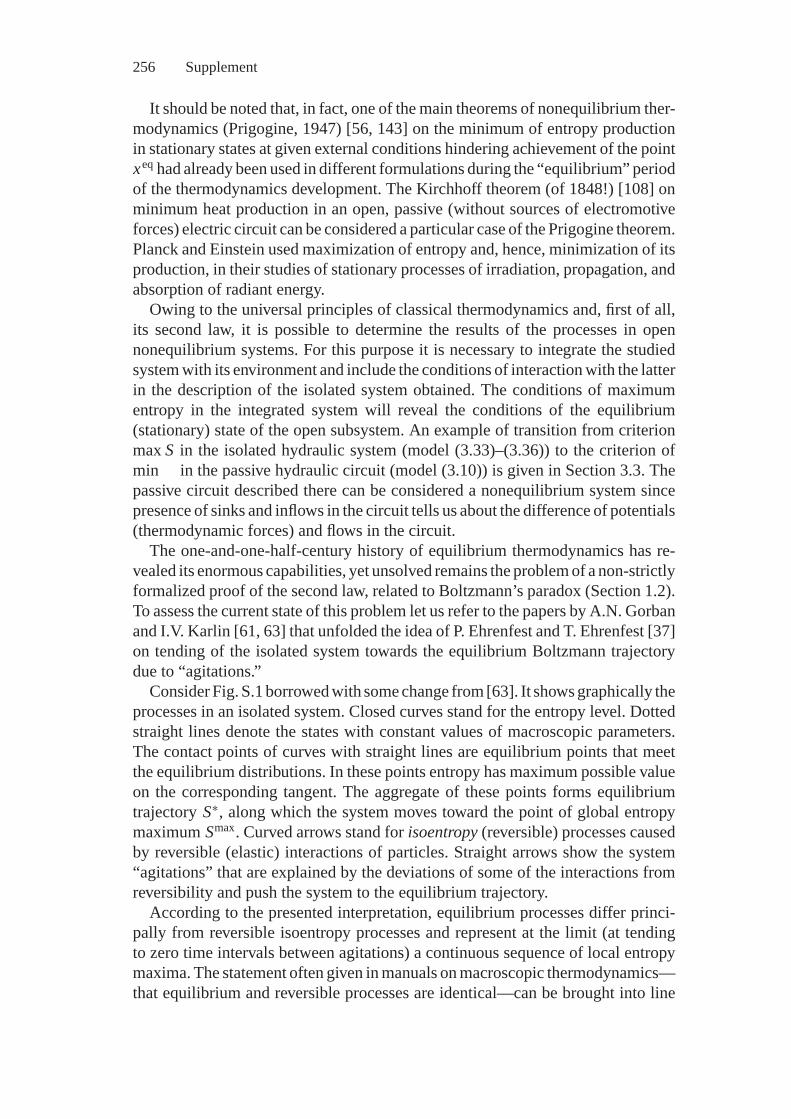
256 Supplement
It should be noted that, in fact, one of the main theorems of nonequilibrium ther-modynamics (Prigogine, 1947) [56, 143] on the minimum of entropy productionin stationary states at given external conditions hindering achievement of the pointxeq had already been used in different formulations during the “equilibrium” periodof the thermodynamics development. The Kirchhoff theorem (of 1848!) [108] onminimum heat production in an open, passive (without sources of electromotiveforces) electric circuit can be considered a particular case of the Prigogine theorem.Planck and Einstein used maximization of entropy and, hence, minimization of itsproduction, in their studies of stationary processes of irradiation, propagation, andabsorption of radiant energy.
Owing to the universal principles of classical thermodynamics and, first of all,its second law, it is possible to determine the results of the processes in opennonequilibrium systems. For this purpose it is necessary to integrate the studiedsystem with its environment and include the conditions of interaction with the latterin the description of the isolated system obtained. The conditions of maximumentropy in the integrated system will reveal the conditions of the equilibrium(stationary) state of the open subsystem. An example of transition from criterionmax S in the isolated hydraulic system (model (3.33)–(3.36)) to the criterion ofmin in the passive hydraulic circuit (model (3.10)) is given in Section 3.3. Thepassive circuit described there can be considered a nonequilibrium system sincepresence of sinks and inflows in the circuit tells us about the difference of potentials(thermodynamic forces) and flows in the circuit.
The one-and-one-half-century history of equilibrium thermodynamics has re-vealed its enormous capabilities, yet unsolved remains the problem of a non-strictlyformalized proof of the second law, related to Boltzmann’s paradox (Section 1.2).To assess the current state of this problem let us refer to the papers by A.N. Gorbanand I.V. Karlin [61, 63] that unfolded the idea of P. Ehrenfest and T. Ehrenfest [37]on tending of the isolated system towards the equilibrium Boltzmann trajectorydue to “agitations.”
Consider Fig. S.1 borrowed with some change from [63]. It shows graphically theprocesses in an isolated system. Closed curves stand for the entropy level. Dottedstraight lines denote the states with constant values of macroscopic parameters.The contact points of curves with straight lines are equilibrium points that meetthe equilibrium distributions. In these points entropy has maximum possible valueon the corresponding tangent. The aggregate of these points forms equilibriumtrajectory S∗, along which the system moves toward the point of global entropymaximum Smax. Curved arrows stand for isoentropy (reversible) processes causedby reversible (elastic) interactions of particles. Straight arrows show the system“agitations” that are explained by the deviations of some of the interactions fromreversibility and push the system to the equilibrium trajectory.
According to the presented interpretation, equilibrium processes differ princi-pally from reversible isoentropy processes and represent at the limit (at tendingto zero time intervals between agitations) a continuous sequence of local entropymaxima. The statement often given in manuals on macroscopic thermodynamics—that equilibrium and reversible processes are identical—can be brought into line
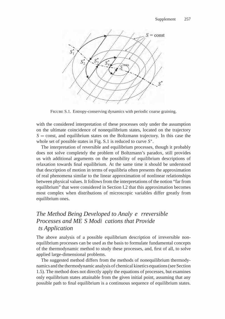
Supplement 257
Figure S.1. Entropy-conserving dynamics with periodic coarse graining.
with the considered interpretation of these processes only under the assumptionon the ultimate coincidence of nonequilibrium states, located on the trajectoryS = const, and equilibrium states on the Boltzmann trajectory. In this case thewhole set of possible states in Fig. S.1 is reduced to curve S∗.
The interpretation of reversible and equilibrium processes, though it probablydoes not solve completely the problem of Boltzmann’s paradox, still providesus with additional arguments on the possibility of equilibrium descriptions ofrelaxation towards final equilibrium. At the same time it should be understoodthat description of motion in terms of equilibria often presents the approximationof real phenomena similar to the linear approximation of nonlinear relationshipsbetween physical values. It follows from the interpretations of the notion “far fromequilibrium” that were considered in Section I.2 that this approximation becomesmost complex when distributions of microscopic variables differ greatly fromequilibrium ones.
The Method Being Developed to Analy e rreversibleProcesses and ME S Modi cations that Providets Application
The above analysis of a possible equilibrium description of irreversible non-equilibrium processes can be used as the basis to formulate fundamental conceptsof the thermodynamic method to study these processes, and, first of all, to solveapplied large-dimensional problems.
The suggested method differs from the methods of nonequilibrium thermody-namics and the thermodynamic analysis of chemical kinetics equations (see Section1.5). The method does not directly apply the equations of processes, but examinesonly equilibrium states attainable from the given initial point, assuming that anypossible path to final equilibrium is a continuous sequence of equilibrium states.
258 Supplement
These states do not depend on the prehistory of their attainment and the time vari-able can be excluded from their description. Correspondingly, the nonequilibriumstates are interpreted as states of intermediate partial equilibria.
Along with the indicated physical assumptions, mathematical assumptionson convexity (concavity) of the characteristic thermodynamic function andconvexity of the system of constraints—i.e., on reducibility of the problem solvedto one of convex programming—are made. Reducibility can also be reached byapproximation of the used mathematical expressions. When the constraints onkinetics and transfer processes are applied, in addition to the other constraints,these processes are presumed to satisfy autonomous differential equations of typex = f (x).
The time variable can be excluded from motion descriptions by two procedures.The first is dealt with in Section 1.5 and in [87, 89]. By this procedure, variableson the right-hand sides of autonomous equations are represented as functions ofthermodynamic potentials and then the transformed right-hand sides are substitutedinto the expression for the overall characteristic thermodynamic function of thesystem. A condition of the monotonic change of the latter is included in MEIS,and its corresponding modification is described in [86, 87, 89].
MEIS construction on the basis of the first procedure involves essential diffi-culties. Indeed, one of the difficulties is that the main variants of the model ofextreme intermediate states ((2.38)–(2.42), (2.43)–(2.50)) assume knowledge of alist of variables rather than the mechanism of the overall process. Since, in general,motion equations that limit the thermodynamic attainability region include onlysome of the sought variables, there is a need to formulate an expression for thecharacteristic function depending variously on different groups of arguments.
The second procedure, one which entails the exclusion of τ , is to directly applyeither the right-hand sides of motion equations orthe integrals of these equationsor linear approximations of them. This procedure is much simpler compared tothe first one. Currently, MEIS with rate constraints are applied on the basis of thesecond procedure only.
For the physicochemical systems with the fixed T , P , and y a new modificationhas the following form:
Find
max
(F(x) =
∑j∈J ext
c j x j
)= F
(xext) (S.1)
subject to
Ax = b, (S.2)Dt (y) = {x : x ≤ y} , (S.3)
ϕ (x) ≤ �, (S.4)G (x) = ∑
jG j (x) x j , (S.5)
x j ≥ 0, (S.6)
Supplement 259
where � is a given limiting value of the expression for a process that decreasesDt (y).
The presence of inequality (S.4) restricting the values of expressions for thelimiting processes distinguishes the model (S.1)–(S.6) from model (2.38)–(2.42).In some respects the model (S.1)–(S.6) has some advantages over the models ofnonequilibrium thermodynamics and over the thermodynamic transformations ofthe motion equations. Transition from the analysis of trajectories to the analysisof states substantially reduces the amount of necessary initial information. Thus,in a general case, it is unnecessary to know the whole mechanism of the studiedprocess, i.e., its elementary or formally simple stages. There is a need only forthe initial information on limiting motion equations. Besides, the applied mathe-matical technique is appreciably simplified. Differential equations are substitutedby algebraic and transcendent ones. In this case it appears possible to describeby the finite values spatially inhomogeneous systems, ones in which the intensiveparameters experience changes in some directions (see Section 2.3). Formulationof the problem in terms of mathematical programming allows the applied modelto be supplemented with diverse equality and inequality constraints to take intoaccount specific features of the considered phenomenon (see Section 2.2).
Examples of Equilibrium Description ApplicationThe efficiency of MEIS-type model with descriptions of motion will be illustratedon examples of inclusion of constraints on chemical reaction rates and analysis ofstationary and nonstationary flow distributions in hydraulic circuits.
At first we will deal with construction and application of MEIS modifications(S.1)–(S.6) on the simplest example of isomerization reaction for the system withthree components, x1, x2 and x3, that was described in Section 2.2. The processmechanism consists of the stages
x1 → x2 and x2 → x3
and the constraints on rate of the second of them, T , P , and the vector y = (1, 0, 0)T
are given.If the maximum attainable x3 is determined, model (S.1)–(S.6) for this example
takes the following form:Find
max x3 (S.7)
subject to
x1 + x2 + x3 = 1, (S.8)Dt (y) = {x : x ≤ y} , (S.9)
k2x2 ≤ �, (S.10)G (x) = ∑
jG j (x) x j , (S.11)
x j ≥ 0. (S.12)
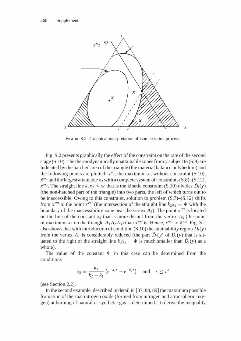
260 Supplement
x
1
2 3
x
x
x2 2
Ψ
Figure S.2. Graphical interpretation of isomerization process.
Fig. S.2 presents graphically the effect of the constraint on the rate of the secondstage (S.10). The thermodynamically unattainable zones from y subject to (S.9) areindicated by the hatched area of the triangle (the material balance polyhedron) andthe following points are plotted: xeq, the maximum x3 without constraint (S.10),xext and the largest attainable x3 with a complete system of constraints (S.8)–(S.12),xext. The straight line k2x2 ≤ � that is the kinetic constraint (S.10) divides Dt (y)(the non-hatched part of the triangle) into two parts, the left of which turns out tobe inaccessible. Owing to this constraint, solution to problem (S.7)–(S.12) shiftsfrom xext to the point xext (the intersection of the straight line k2x2 = � with theboundary of the inaccessibility zone near the vertex A3). The point xext is locatedon the line of the constant x3 that is more distant from the vertex A3 (the pointof maximum x3 on the triangle A1 A2 A3) than xext is. Hence, xext < xext. Fig. S.2also shows that with introduction of condition (S.10) the attainability region Dt (y)from the vertex A1 is considerably reduced (the part Dt (y) of Dt (y) that is sit-uated to the right of the straight line k2x2 = � is much smaller than Dt (y) as awhole).
The value of the constant � in this case can be determined from theconditions
x2 = k1
k2 − k1
(e−k1τ − e−k2τ
)and τ ≤ τ b
(see Section 2.2).In the second example, described in detail in [87, 88, 89] the maximum possible
formation of thermal nitrogen oxide (formed from nitrogen and atmospheric oxy-gen) at burning of natural or synthetic gas is determined. To derive the inequality
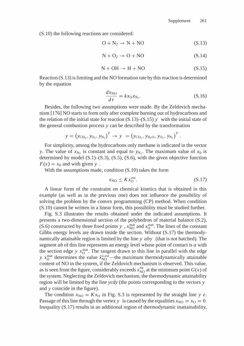
Supplement 261
(S.10) the following reactions are considered:
O + N2 → N + NO (S.13)
N + O2 → O + NO (S.14)
N + OH → H + NO (S.15)
Reaction (S.13) is limiting and the NO formation rate by this reaction is determinedby the equation
dxNO
dτ= kxOxN2 . (S.16)
Besides, the following two assumptions were made. By the Zeldovich mecha-nism [176] NO starts to form only after complete burning out of hydrocarbons andthe relation of the initial state for reaction (S.13)–(S.15) y with the initial state ofthe general combustion process y can be described by the transformation
y = (yCH4 , yO2 , yN2
)T → y = (yCO2 , yH2O, yO2 , yN2
)T.
For simplicity, among the hydrocarbons only methane is indicated in the vectory. The value of xN2 is constant and equal to yN2 . The maximum value of x0 isdetermined by model (S.1)–(S.3), (S.5), (S.6), with the given objective functionF(x) = x0 and with given y .
With the assumptions made, condition (S.10) takes the form
xNO ≤ K xextO . (S.17)
A linear form of the constraint on chemical kinetics that is obtained in thisexample (as well as in the previous one) does not influence the possibility ofsolving the problem by the convex programming (CP) method. When condition(S.10) cannot be written in a linear form, this possibility must be studied further.
Fig. S.3 illustrates the results obtained under the indicated assumptions. Itpresents a two-dimensional section of the polyhedron of material balance (S.2),(S.6) constructed by three fixed points y , xmat
NO and xmatO . The lines of the constant
Gibbs energy levels are drawn inside the section. Without (S.17) the thermody-namically attainable region is limited by the line y aby (that is not hatched). Thesegment ab of this line represents an energy level whose point of contact is a withthe section edge y xmat
O . The tangent drawn to this line in parallel with the edgey xmat
O determines the value xz.extNO —the maximum thermodynamically attainable
content of NO in the system, if the Zeldovich mechanism is observed. This value,as is seen from the figure, considerably exceeds xeq
NO at the minimum point G(x) ofthe system. Neglecting the Zeldovich mechanism, the thermodynamic attainabilityregion will be limited by the line ycdy (the points corresponding to the vectors yand y coincide in the figure).
The condition xNO = K xO in Fig. S.3 is represented by the straight line y e.Passage of this line through the vertex y is caused by the equalities xNO = xO = 0.Inequality (S.17) results in an additional region of thermodynamic inattainability,
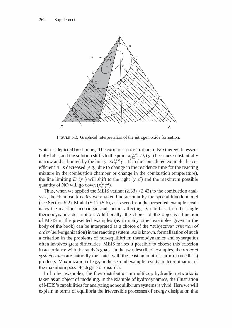
262 Supplement
a
b
x,
x ,
x ,
x
x
x
x
x,
,
Figure S.3. Graphical interpretation of the nitrogen oxide formation.
which is depicted by shading. The extreme concentration of NO therewith, essen-tially falls, and the solution shifts to the point xz.ext
NO . Dt (y ) becomes substantiallynarrow and is limited by the line y axz.ext
NO y . If in the considered example the co-efficient K is decreased (e.g., due to change in the residence time for the reactingmixture in the combustion chamber or change in the combustion temperature),the line limiting Dt (y ) will shift to the right (y e′) and the maximum possiblequantity of NO will go down (x ′z.ext
NO ).Thus, when we applied the MEIS variant (2.38)–(2.42) to the combustion anal-
ysis, the chemical kinetics were taken into account by the special kinetic model(see Section 5.2). Model (S.1)–(S.6), as is seen from the presented example, eval-uates the reaction mechanism and factors affecting its rate based on the singlethermodynamic description. Additionally, the choice of the objective functionof MEIS in the presented examples (as in many other examples given in thebody of the book) can be interpreted as a choice of the “subjective” criterion oforder (self-organization) in the reacting system. As is known, formalization of sucha criterion in the problems of non-equilibrium thermodynamics and synergeticsoften involves great difficulties. MEIS makes it possible to choose this criterionin accordance with the study’s goals. In the two described examples, the orderedsystem states are naturally the states with the least amount of harmful (needless)products. Maximization of xNO in the second example results in determination ofthe maximum possible degree of disorder.
In further examples, the flow distribution in multiloop hydraulic networks istaken as an object of modeling. In the example of hydrodynamics, the illustrationof MEIS’s capabilities for analyzing nonequilibrium systems is vivid. Here we willexplain in terms of equilibria the irreversible processes of energy dissipation that
Supplement 263
are associated with viscosity and thermal conduction. In the examples we discuss,this problem is solved more easily owing to the assumption on the one-dimensionalflows, as systems with such flows are potential systems (see Sections I.25 and 3.3).
First we will make some comments on the examples in Sections 3.3 and 3.4. Weconsider the derivation of the model of an open passive circuit with the Lagrangefunction
L =n p∑
i=1i xβ+1
i −m−1∑j=1
λ j
(∑i∈ j
a ji xi
)
from the model of the closed active circuit (3.33)–(3.36). This derivation can beconsidered a special case of Prigogine’s theorem for non-equilibrium processes,which was mentioned above.
The results of calculating the circuit diagram in Fig. 3.4 (see Table 3.2,variant 3) show the possibility of determining from the condition of isolated systemequilibrium (max S) the order levels in open subsystems it comprises (the turbu-lent flow in branches 1–15 and the laminar flow in branch 16). In fact, the typeof closing relations in this case was given in advance. However, optimization ofthese relations using the second law for circuits with lumped parameters involvesonly mathematical difficulties.
In Section 3.4 derivations of closing relations for nonideal multiphase and multi-component liquids were illustrated by techniques of constructing one-dimensionalpotential models of irreversible flow of a viscous fluid. The sketch of equilibriumdescriptions of fire spreading in systems of air exchange in buildings as presentedin this section surely belong to modeling of irreversible processes.
Nonstationary flow distribution in a hydraulic network will be the last example[89, 93]. The Navier–Stokes equation determining the equilibrium of forces affect-ing liquid flow limits the region of attainable states in this example. For turbulentflow of an incompressible liquid this equation takes the following form, takinginto account forces of pressure, friction, and inertia only:
−dPd�
= λρw2
2d + ρdw
dτ. (S.18)
As a result of elementary transformations we pass from (S.18) to the expression
dxdτ
= πd2
4ρPbr − 2λ
πd3 x2 = γ br Pbr − γ frx2 (S.19)
where x is the volumetric flow rate; Pbr is the specific pressure loss in the branch;γ br and γ fr are coefficients.
Some comments are required before we present MEIS of non-stationary flowdistribution by using equation (S.19). Time-independence of the right-hand sideof equation (S.19) can be interpreted as follows. At any section of hydraulic net-work branch and at any time all flow characteristics, in particular, thermodynamicfunctions (enthalpy, entropy, and others) fully depend on the current state and donot depend explicitly on τ . If the flows are isothermal (1
/T is constant), study of
264 Supplement
the entropy behavior can be substituted by study of enthalpy behavior. Variationin the enthalpy of the network branches at ρ = const and w = const is reduced tovariation in the potential energy (pressure).
Under the assumptions made and the made choice of extreme pressure at thegiven node of the scheme as the objective function MEIS for the closed network(without sources and sinks) takes the form:
Find
ext(Pr = ePm + Pbr
q − Pmovq
)(S.20)
subject to
Axk = 0, (S.21)n∑
i=1
∣∣Pbr.ki
∣∣ (γ bri Pbr.k
i − γ fri xk2
i
)≥ 0, (S.22)
n∑i=1
Pmovi
∣∣xki∣∣ −
n∑i=1
∣∣Pbr.ki xk
i∣∣�i = 0, (S.23)
P = ePm − A−1q
(Pbr
q − Pmovq
)(S.24)
where P is the vector of pressure at the nodes; Pm is the fixed pressure at nodej = m; Pmov
i is the effective head in the i th branch; Pbrq and Pmov
q are the vectorsof pressure drop and the effective pressure in the branches of the “circuit tree” qthat includes the paths from nodes j = 1, . . . , m − 1 to node m (see Section 3.3,model (3.45)–(3.48)); Aq is the matrix of “paths” that corresponds to the circuittree q; k is an index of iteration of the computational process; and r is an index ofthe node, at which the extreme pressure is sought.
Equation (S.21) represents the material balance of a closed network. Inequality(S.22) accounts for the condition of monotone nondecrease of entropy. Note that theexpression in parentheses on the left-hand side of (S.22) is the right-hand side of theNavier–Stokes equation, i.e., it is the time–derivative of the flow. Equality (S.23)is the energy balance of the network for each equilibrium state considered in theiterative calculation. Equation (S.24) is applied to calculate nodal pressures that arealso sought variables along with flows in the branches. The use of absolute valuesof variables in (S.22) and (S.23) is explained by the fact that energy dissipationdoes not depend on the direction of flows.
Physically, the accepted problem statement may (for example) consist of deter-mining maximum pressure rise at fast flow closure in any branch or its maximumdrop at pipe break. Of course, other statements on the problem of searching forpartial equilibria in multiloop hydraulic systems—problems that involve analysisof normal or emergency nonstationary flow distribution—are also possible.
The form of model (S.20)–(S.24) shows that it is written for conditions where“fast” disturbances proceed so slowly that frictional forces have time to revealthemselves, i.e., the liquid does not become ideal. Basic difficulties emerge whendescribing “instantaneous” disturbances leading to wave processes and, in somecases, to hydraulic shocks. The authors have taken only the first steps in the analysisof the presented problem; however, these steps offer hope for its successful solution.
Supplement 265
Derivation of the hydraulic shock equation from the Lagrange equilibrium equationas one of the steps to the solution is described in Section 1.3.
ConclusionWe reveal the capabilities of descriptions of equilibrium, not to oppose currentlyrecognized scientific direction (such as nonequilibrium thermodynamics and syn-ergetics [67, 143]), but to display the expediency of supplementing new approachesby old, “good” models of equilibria.
Nonequilibrium thermodynamics and synergetics involve undeniable progressin: the explanation of many of the phenomena in transfer processes; the develop-ment of the theories of self-organization; and the ordering in physical, chemical,biological, and social systems. Introduction of the methods of classical thermody-namics into these areas is advisable primarily for solving large-dimensional appliedproblems. Note that it was precisely the equilibrium thermodynamic models thatwere used in the first half of the 20th century to create numerous computationalsystems for computational studies in energy, metallurgy, astronautics, geology,ecology, and other spheres of science and technology. MEIS offers advantagesover the traditional models of equilibrium thermodynamics in terms of its capabil-ities to account for constraints on kinetics and transfer processes, i.e., to estimatefeasibility of equilibria sought.
Currently, we can construct computational MEIS-based algorithms for specificproblems using the sufficiently detailed analysis of MEIS’s mathematical proper-ties and its reducibility to the convex programming problem. We have implementedthe basic units of a commercial computational software, one that is available tousers and that can easily be supplemented with the auxiliary units.
However, to make the equilibrium models of nonequilibrium systems acces-sible to a wide circle of researchers and engineers, we need to “detailize” themodels to fit the basic processes of matter, energy, impulse, and charge transfer.For the time being, models of extreme intermediate states have been worked outin certain detail only in descriptions of chemical kinetics and one-dimensionalhydrodynamics (for multiloop systems though). Strict thermodynamic descrip-tion of different “motions,” in turn, requires that mathematical interrelations be-tween equilibrium models of mechanics and thermodynamics, and between theformalisms of equilibrium and nonequilibrium thermodynamics, be elucidated.The authors are currently investigating this problem.
References
1. Aerosol and Climate/ Edited by K.Ya. Kondratiev. Leningrad: Gidrometeoizdat, 1991.541 p. (in Russian)
2. Afanasieva-Ehrenfest T.A. Irreversibility, homogeneity and second principle of ther-modynamics. J. Appl. Phys.—1928; Vol. 5, 3–4: P.3–30. (in Russian)
3. Altshul A.D. Hydraulics and Aerodynamics. Moscow: Stroyizdat, 1975. 323 p. (inRussian)
4. Antsiferov E.G. Application of mathematical programming methods to the analysis ofthermodynamic systems: Abstract of doctoral thesis. Moscow, 1991. 30 p. (in Russian)
5. Antsiferov E.G., Ashchepkov L.T. and Bulatov V.P. Optimization methods and theirapplications. Part 1. Mathematical Programming. Novosibirsk: Nauka, 1990. 158 p.(in Russian)
6. Antsiferov E.G. and Bulatov V.P. Simplex embedding method in convex programming.J. Calculus Math. Math Phys. 1987; Vol. 27 (No. 3): P.377–384. (in Russian)
7. Antsiferov E.G., Kaganovich B.M. and Semeney P.T. Search for intermediate ther-modynamic states of physicochemical systems. In: Numerical Methods of Anal-ysis and their Applications. Irkutsk: Siberian Energy Institute, 1987. P.150–170.(in Russian)
8. Antsiferov E.G., Kaganovich B.M. and Yablonsky G.S. Thermodynamic limitationsin searching for regions of optimal performance of complex chemical reactions (ex-amplified by conversion of hydrocarbons). React. Kinet. Catal. Lett. 1988; Vol. 37(No. 1): P.57–61.
9. Sinyarev G.B., Vatolin M.A., Trusov B.G. and. Moiseev G.K. Application of Com-puters to Thermodynamic Calculation of Metallurgical processes. Moscow: Nauka,1982. 263 p. (in Russian)
10. Arnold V.I. On representation of functions of multiple variables as the superpositionof functions of lesser number of variables. In: Mathematical Enlightenment. Edition3. Moscow: Gos. fiz.-mat. Li, 1958. P.41–61. (in Russian)
11. Asaturov M.L., Budyko M.I. and Vinnikov K.Ya. Volcanoes, Stratosphere Aerosoland Planet Climate. – Leningrad: Gidrometeoizdat, 1986. 255 p. (in Russian)
12. Atkinson R. and Arey J. Atmospheric chemistry of gas-phase polycyclic aromatichydrocarbons: Formation of atmospheric mutagens.Environ. Health Perspect. Suppl.1994; Vol. 102 (Suppl 4): P.117–126.
13. Atkinson R., Baulch D.L. and Cox R.A. Evaluated kinetic and photochemical data foratmospheric chemistry. J. Phys. Chem. Ref. Data. 1989; Vol. 18 (No. 2): P.881–1097.
266
References 267
14. Atmosphere Protection from Industrial Pollution: Reference-book, edited by S. Calvertand G.B. Inglund.—Moscow: Metallurgiya, 1988; Vol. 1: 760 p; Vol. 2: 712 p. (inRussian)
15. Atmosphere: Reference-book (reference data, models). Leningrad: Gidrometeoizdat,1991. 509 p. (in Russian)
16. Balyshev O.A. Nonstationary models in hydraulic circuits theory: Abstract of doctoralthesis. Irkutsk, 1998. 48 p. (in Russian)
17. Balyshev O.A., Kaganovich B.M. and Merenkov A.P. Pipeline systems of heat andwater supply as dynamic models of hydraulic circuits. v. A . Energetika. 1996;(No. 2): P.96–104. (in Russian)
18. Balyshev O.A. and Tairov E.A. The Analysis of Transient and Stationary Processes inPipeline Systems (Theoretical and Experimental Aspects). Novosibirsk: Nauka, 1998.164 p. (in Russian)
19. Bazaraa M.S., Sherali H.D. and Shetty C.M. Nonlinear Programming: Theory andAlgorithms. New-York: John Willey Sons, Inc. 1993.
20. Bazarov I.P. Thermodynamics. Moscow: Vysshaya shkola, 1991. 376 p. (in Russian)21. Boltzmann L. Uber die Beziehung zwishen dem zweiten Hauptsatze der mechanischen
Warmetheorie und der Wahrscheinlichkeitsrechnung respective den Satzen uber dasWarmegleichgewicht. ien. Akad. Sit ungsber. 1878; Bd. 76: S.373–435.
22. Boreskov G.K. Catalysis: uestions of Theory and Practice. Novosibirsk: Nauka,1987. 536 p. (in Russian)
23. Born M. Kritische Betrachtungen zur traditionellen Darstellung der Thermodynamik.Physic, Zschr. 1920; 22: 218–224, 249–254, 282–286.
24. Bowen R.M. Thermochemistry of reacting materials. J. Chem. Phys. 1968; Vol. 49(4): P.1625–1637.
25. Brimblecombe P. Air Composition and Chemistry. Cambridg: Cambridge UniversityPress, 1986.
26. Bugaenko L.T., Kuzmin M.G. and Polak L.S. High Energy Chemistry. N.Y.-Toronto-Sydney-Tokyo-Singapore: Ellis Horwood and Prentice Hall, 1993. 403 p.
27. Caratheodory C. Untersuchungen uber die Grundlagen der Thermodynamik. Math.Ann. 1909; 61: S.355–390.
28. Chemical Applications of Topology and Graph Theory, edited by R.B. King.Amsterdam-Oxford-New York-Tokyo: Elsevier, 1983. 560 p.
29. Coleman B.D. and Gurtin M.E. Thermodynamics with internal state variables.J. Chem.Phys. 1967; Vol. 47: P.597–613.
30. Combustion chemistry, edited by W.G. Gardiner. New York: Springer-Verlag, 1984.464 p.
31. Conrad R. Flux of NOx between soil and atmosphere: Importance of microbialmetabolism. In: Denitrification in Soil and Sediment, edited by N.P. Revsbech and J.Sorensen. New York: Plenum Press, 1990. P.105–128.
32. Dantzig G., Johnson S. and White W. A linear programming approach to the chemicalequilibrium problem.Manag. Sci. 1958; Vol. 5 (No. 1): P.38–43.
33. Dantzig G.B. Linear Programming and Extensions. Princeton: Princeton UniversityPress, 1963. 460 p.
34. Dikin I.I. Iterative solution of linear and quadratic programming problems. Papers ofAS USSR. 1967; Vol. 174 (No. 4): P.747–748. (in Russian)
35. Dikin I.I. and Zorkaltsev V.I. Iterative Solution of Linear Mathematical ProgrammingProblems. Novosibirsk: Nauka, 1986. 144 p. (in Russian)
268 References
36. Dovgaluk U.A. and Ivlev L.S. Physics of Aqueous and Other Atmospheric Aerosols.S.-Petersburg: S.-Petersburg University, 1998. (in Russian)
37. Ehrenfest P. Collected Scientific Papers. North-Holland, Amsterdam: 1959. P.213–300.
38. Einstein A. Beitrage zur uantentheorie. Dtsch. Phys. Ges. 1914; 16: S.820–828.39. Einstein A. Deduction thermodynamique de la loi de l’equivalence photochemique.
J. Phys. Ser. 1913; 111: S.277–282.40. Einstein A. Uber die von der molekularkinetischen Theorie der Warme geforderte
Bewegung von in ruhenden Flussigkeiten suspendierten Teilchen. Ann. Phys. 1905;17: S.549–560.
41. Einstein A. Zur Theorie der Brownschen Bewegung. Ann. Phys. 1906; 19: S.371–381.42. Einstein A. Elementare Theorie der Brownschen Bewegung. s. Ekrochem. 1908; 4:
S.235–239.43. Einstein A. Theorie der Opaleszenz von homogenen Flussigkeiten und
Flussigkeitsgemischen in der Nahe des krittischen Zustandes. Ann. Phys. 1910; 33:S.1275–1298.
44. Feinberg M. On chemical kinetics of a certain class. Arch. Rat. Mech. Anal. 1972; Vol.46 (No. 1): P.1–41.
45. Feinberg M. Recent results in optimal reactor synthesis region theory.Chem. Eng. Sci.1999; Vol. 54 (No. 7): P.2535–2544.
46. Feinberg M. and Hildebrant D. Optimal reactor design from a geometric viewpoint—1. Universal properties of the attainable region. Chem. Eng. Sci. 1997; Vol. 52 (No.10): P.1637–1665.
47. Feinberg M. and Horn F. Dynamics of open chemical systems and the algebraicstructure of the underlying reaction network.Chem. Eng. Sci. 1974; Vol. 29: P.775–787.
48. Fenimore C.P. Formation of nitric oxide from fuel nitrogen in ethylene flames. Com-bust. Flames. 1972; Vol. 19 (No. 2): P.289–296.
49. Feynman R.P., Leighton R.B. and Sands M. The Feynman Lectures on Physics.Massachusetts-Palo Alto-London: Addison-Wesley, Inc., 1963.
50. Filippov S.P., Kaganovich B.M. and Pavlov P.P. Thermodynamic modeling of nitrogenoxides formation during coal combustion. nt. J. Energ. Environ. Econ. 1997; Vol. 6(No. 1): P.47–66.
51. Fourier I.B.J. Theorie Analytique de la chaleur. Paris: 1822. 673 p.52. Gantmacher F.R. The Theory of Matrices. American Mathematical Society, 1959.
ISBN: 0821826646.53. Gerasimov Ya.I. and Geidrich V.A. Thermodynamics of Solutions. Moscow: Moscow
State University, 1980. 184 p. (in Russian)54. Gibbs J.W. On the equilibrium of heterogeneous substances. Trans. Connect. Acad.
1876; 3: P.108–248. 1878; 3: P.343–524.55. Gibbs J.W. Statistical Mechanics. bid. P.350–508.56. Glansdorff P. and Prigogine I. Thermodynamics of Structure, Stability and Fluctua-
tions. New York: Wiley. 1971. 280 p.57. Glasser D., Hildebrant D. and Godorr S. The attainable region for segregated, maxi-
mum mixing, and other reactor models. nd. Eng. Res. 1994; Vol. 33 (No. 5): P.1136–1144.
58. Gorban A.N. Equilibrium encircling. Novosibirsk: Nauka, 1984. 226 p. (in Russian)59. Gorban A.N. Methods for qualitative study of chemical kinetics equations. Chislennye
Metody Mekhaniki Sploshnoi Sredy. 1979; Vol. 10 (No. 4): P.42–59.
References 269
60. Gorban A.N., Bykov V.I. and Yablonsky G.S. Sketches on Chemical Relaxation.Novosibirsk: Nauka, 1986. 236 p. (in Russian)
61. Gorban A.N. and Karlin I.V. Invariant manifolds for physical and chemical kinetics.Lecture Notes in Physics. Berlin-Heidelberg: Springer, Vol. 660. 2005.
62. Gorban A.N., Karlin I.V. and Zinovyev A.Ju. Constructive methods of invariantmanifolds for kinetic problems. Phys. Reports 396, 4–6: 2004. P. 197–403. Preprintonline.
63. Gorban A.N., Karlin I.V., Ottinger H.C. and Tatarinova J.J. Ehrenfest’s argumentextended to a formalism of nonequilibrium thermodynamics. Phys. Rev. E. 2001; Vol.63: P.1–6.
64. Gorban A.N., Yablonskii G.S. and Bykov V.I. The path to equilibrium. nt. Chem.Engn. 1982; Vol. 22 (No. 2): P.368–375.
65. Gradstein I.S. and Ryzhik I.M. Tables of Integrals, Sums, Series and Products.Moscow: Gos. fiz.-mat. izdat., 1962. 1100 p. (in Russian)
66. Grishin A.M. Mathematical Modeling of Forest Fires and New Methods of TheirExtinguishing. Novosibirsk: Nauka, 1992. 408 p. (in Russian)
67. Haken H. Advanced Synergetics. Instability Hierarchies of Self-Organizing Systemsand Devices. Berlin-Heidelberg-New-York-Tokyo: Springer-Verlag, 1983.
68. Handbook of Air Pollution Technology, edited by S. Calvert and H.M. Englund. New-York: John Wiley Sons, Inc., 1984. 850 p.
69. Hilbert D. Gesammelte Abhandlungen. B. 3, 1935. S.290–329.70. Hildebrant D. and Glasser D. Predicting phase and chemical equilibrium using the
convex hull of the Gibbs energy. Chem. Eng. J. (Lausanne). 1994; Vol. 54 (No. 3):P.187 –197.
71. Horn F. and Jackson R. General mass action kinetics. Arch. Rat. Mech. Anal. 1972;Vol.47 (No. 2): P.81–116.
72. Horn R.A. and Johnson C.R. Matrix Analysis. Cambridge [Cambridgeshire]-NewYork: Cambridge University Press, 1985.
73. Izmailov N.A. Electrochemistry of solutions. Moscow: Himiya, 1976. 130 p. (in Rus-sian)
74. Juda-Rezler K. Classification and characteristics of air pollution models. In: Chemistryfor the Protection of the Environment, edited by L. Pawlowski et al. New York: 1991.P.51–72.
75. Kaganovich B.M., Merenkov A.P. and Sumarokov S.V. Physico-mathematical Aspectsin Developing Hydraulic Circuits Theory. Irkutsk: Siberian Energy Institute, 1993.37 p. (in Russian)
76. Kaganovich B.M. Discrete Optimization of Heat Supply Systems. Novosibirsk:Nauka, 1978. 88 p. (in Russian)
77. Kaganovich B.M. Extremality criteria in hydraulic circuits theory. Preprint No. 15.Irkutsk: Energy Systems Institute, 1997. 22 p. (in Russian)
78. Kaganovich B.M. Thermodynamic interpretations of extreme models of flow distri-bution in hydraulic circuits. v. A . Energetika. 2000; No. 2: P.77–83. (in Russian)
79. Kaganovich B.M. Thermodynamics of Circuits. Irkutsk: Siberian Energy Institute,1991. 35 p. (in Russian)
80. Kaganovich B.M. and Filippov S.P. Development of equilibrium thermodynamic mod-els for studying technical and environmental problems in energy. nt. J. Global Energyssues. 2003; Vol. 20 (No. 4): P.326–339.
81. Kaganovich B.M. and Filippov S.P. Equilibrium Thermodynamics and MathematicalProgramming. Novosibirsk: Nauka, 1995. 236 p. (in Russian)
270 References
82. Kaganovich B.M., Filippov S.P. and Antsiferov E.G. Efficiency of Energy Tech-nologies: Thermodynamics, Economics, Forecasts. Novosibirsk: Nauka, 1989. 256 p.(in Russian)
83. Kaganovich B.M., Filippov S.P. and Antsiferov E.G. Modeling of ThermodynamicProcesses. Novosibirsk: Nauka, 1993. 101 p. (in Russian)
84. Kaganovich B.M., Filippov S.P. and Antsiferov E.G. Studies of the environmentalpollution using thermodynamic models. nt. J. Energ. Environ. Econ. 1992; Vol. 2(No. 1): P.7–13.
85. Kaganovich B.M., Filippov S.P. and Pavlov P.P. Thermodynamic Modeling on Graphs.Irkutsk: Energy Systems Institute, 1998. Preprint No. 6. 30 p. (in Russian)
86. Kaganovich B.M., Filippov S.P., Shamansky V.A. and Shirkalin I.A. On the feasibilityof equilibria in processes of substance and energy conversion. v. A . Energetika.2004; No. 5: P.123–131. (in Russian)
87. Kaganovich B.M., Keiko A.V., Shamansky V.A. and Shirkalin I.A. Analysis of Fea-sibility of Thermodynamic Equilibria in Physicotechnical systems. Irkutsk: EnergySystems Institute, 2004. Preprint No. 10. 61 p. (in Russian)
88. Kaganovich B.M., Keiko A.V., Shamansky V.A. and Shirkalin I.A. Description ofnon-equilibrium processes in energy problems by the equilibrium thermodynamicsmethods. v. A . Energetika. 2006. No. 3. (in Russian)
89. Kaganovich B.M., Keiko A.V., Shamansky V.A. and Shirkalin I.A. On the area ofequilibrium thermodynamics application. Proc. ASME 2004 Int. Mech. Eng. Congr.Nov. 13–19, 2004, Anaheim, California-USA.
90. Kaganovich B.M., Kuchmenko E.V., Shamansky V.A. and Shirkalin I.A. Thermody-namic modeling of phase transitions in multicomponent systems. v. A . Energetika.2005; No. 2: P.114–121. (in Russian)
91. Kaganovich B.M., Merenkov A.P. and Balyshev O.A. Elements of HeterogeneousHydraulic Circuits Theory. Novosibirsk: Nauka, 1997. 120 p. (in Russian)
92. Kaganovich B.M., Merenkov A.P., Sumarokov S.V. and Shirkalin I.A. Flow distribu-tion in networks and extreme principles of mechanics and thermodynamics. v. A .Energetika. 1995; No. 5: P.107–115. (in Russian)
93. Kaganovich B.M., Shamansky V.A. and Shirkalin I.A. Analysis of feasibility of equi-libria in multicomponent and multiphase media. Proceedings of N.I. LobachevskyMathematical Center. V. 27. Kazan Mathematical Society. Models of continuum me-chanics. Materials of VII Session of the International school on the models of con-tinuum mechanics. Kazan: Izd. Kazan Math. Soc. 2004. P.136–143. (in Russian)
94. Karmanov V.G. Mathematical Programming. Moscow: Nauka, 1986. 288 p. (in Rus-sian)
95. Karpenko E.I. and Messerle V.E. Introduction into Plasma-Energy Technologies ofusing Solid Fuels. Novosibirsk: Nauka, 1997. 118 p. (in Russian)
96. Karpov I.K. Physico-chemical Modeling in Geochemistry on Computers. Novosibirsk:Nauka, 1981. 247 p. (in Russian)
97. Karpov I.K., Kiselev A.I. and Letnikov F.A. Modeling of Natural Minerals Formationon Computers. Moscow: Nedra, 1976. 256 p. (in Russian)
98. Keck J.C. Rate controlled constrained equilibrium. Prog. Energ. Combust. Sci. 1990.Vol. 16: P.125–154.
99. Keiko A.V. Software for Kinetic Analysis of Thermodynamic Processes. Irkutsk:Siberian Energy Institute, 1996. Preprint No. 5. 46 p. (in Russian)
100. Keiko A.V., Filippov S.P. and Kaganovich B.M. Chemical safety of atmosphere andenergy. Irkutsk: Siberian Energy Institute, 1995. Preprint No. 6. 35 p. (in Russian)
References 271
101. Keiko A.V., Filippov S.P. and Kaganovich B.M. Thermodynamic analysis of secondarypollution of the atmosphere. nt. J. Energy Environ. Econ. 1997; Vol. 4 (No. 4): P.247–260.
102. Keiko A.V., Shirkalin I.A. and Filippov S.P. Calculation Tools for ThermodynamicAnalysis. Irkutsk: Energy Systems Institute, 1999. Preprint No. 4. 47 p. (in Russian)
103. Keiko A.V., Shirkalin I.A. and Svishchov D.A. Prospective modes of low-grade solidfuels processing. v. A . Energetika. 2006; No. 3. (in Russian)
104. Khasilev V.Ya. Elements of the hydraulic circuits theory. v. A SSSR. Energetika itransport. 1964; No. 1: P.69–88. (in Russian)
105. Khasilev V.Ya. Elements of the Hydraulic Circuits Theory: Abstract of Doctoral thesis.Novosibirsk, 1966. 98 p. (in Russian)
106. Khasilev V.Ya. Generalized relationships for technical and economic calcula-tions of heat supply and other networks.Teploenergetika. 1957; No. 1: P.28–32(in Russian).
107. Khasilev V.Ya. On the application of mathematical methods for designing and opera-tion of pipeline systems. v. A SSSR. Energetika i transport. 1971; No. 2: P.18–27.(in Russian)
108. Kirchhoff G.R. Ueber die Anwendbarkeit der Formeln fur die Intensitaten der gal-vanischen Strome in einem Systeme linearer Leiter auf Systeme, die zum Teil ausnicht linearen Leitern bestehen, Ges. Abhandl., Leipzig, Johann Ambrosius Barth,1848. S.33–49.
109. Kirchhoff G.R. Ueber die Bewegung der Elektrizitat in Drahten. Ges. Abhandl.Leipzig: Johann Ambrosius Barth, 1882. S.131–154.
110. Kirchhoff G.R. Ueber eine Ableitung der Ohm’schen Gesetze, welche sich an die The-orie der Elektrostatik anschliesst. Ges. Abhandl. Leipzig: Johann Ambrosius Barth,1882. S.49–55.
111. Kirhchhoff G.R. Ueber den Durchgang eines elektrischen Stromes durch eine Ebene,insbesondere durch eine kreisformige. Ann. Phys. 1845; Bd. 64: S.497–514.
112. Kirhchhoff G.R. Ueber die Auflosung der Gleichungen, auf welche man bei der Unter-suchung der linearen Verteilung galvanischen Strome gefuhrt wird. Ann. Phys. 1847;Bd. 71: S.498–508.
113. Kirillin V.A., Sheindlin A.E. and Spilrain E.E. Thermodynamics of Solutions.Moscow: Energiya, 1980. 287 p. (in Russian)
114. Kirillin V.A., Sychev V.V. and Sheindlin A.E. Technical Thermodynamics. Moscow:Nauka, 1979. 490 p. (in Russian)
115. Krichevsky I.R. Notions and Fundamentals of Thermodynamics. Moscow: Himiya,1970. 439 p. (in Russian)
116. Kronrod A.S. On the functions of two variables. Moscow-Leningrad: Gos. izd. teh.-teor. lit. 1950; V. 5: issue 1(35). P.24–134. (in Russian)
117. Kubo R. Thermodynamics. Amsterdam: North-Holland Publishing Company, 1968.118. Lagrange J. Mechanique Analytique. Paris: la Veuve Desaint, 1788.119. Laktionov L.G. Equilibrium heterogeneous condensation. Leningrad: Gidrometeoiz-
dat, 1988. 160 p. (in Russian)120. Landau L.D. The theory of superfluidity of helium II. h. Ecsp. Teor. Fi . 1941; Vol.11:
592 p.121. Landau L.D. Theory of monomolecular reactions. Phys. . Sowjetunion. 1936; Vol.
10: 67 p.122. Landau L.D.and Lifshitz E.M. Theoretical Physics. Electrodynamics of Continuous
Media. Oxford: Pergamon Press, 1960.
272 References
123. Landau L.D. and Lifshitz E.M. Theoretical Physics. Fluid Mechanics. Oxford: Perg-amon Press, 1959.
124. Landau L.D. and Lifshitz E.M. Theoretical Physics. Mechanics. Oxford: PergamonPress, 1960.
125. Landau L.D. and Lifshitz E.M. Theoretical Physics. Statistical Physics. London: Perg-amon Press, 1959.
126. Landau L.D. and Lifshitz E.M. Theoretical Physics. Theory of Elasticity. Oxford:Pergamon Press, 1959.
127. Lifshitz E.M. and Pitievsky L.P. Theoretical Physics. Physical Kinetics. Moscow:Nauka, 1979; Vol. 10: 527 p. (in Russian)
128. Logan J.A. Nitrogen oxides in the troposphere: Global and regional budgets.J. Geo-phys. Res. 1983; Vol. 88: P.10785–10807.
129. Maxwell J.C. A Treatise on Electricity and Magnetism, edited by W.D. Niven, London:The Clarendon Press, 1891.
130. Merenkov A.P. and Khasilev V.Ya. Theory of Hydraulic Circuits. Moscow: Nauka,1985. 278 p. (in Russian)
131. Merenkov A.P., Sennova E.V. and Sumarokov S.V. Mathematical Modeling and Op-timization of Heat-, Water-, Oil-, and Gas Supply Systems. et al. Novosibirsk: Nauka,1992. 407 p. (in Russian)
132. Merenkov A.P., Khasilev V.Ya. and Kaganovich B.M. Methods and algoritms of cal-culating heat supply networks. Moscow: Energiya, 1978. 176 p. (in Russian)
133. Morachevsky V.G., Golovina E.G. and Tsvetkova A.V. The role of atmospheric pollu-tants in formation of urban fogs and low boundary of clouds. Parameterization of somekinds of indeliberate and directed actions on the atmosphere. Leningrad: LeningradHydrometeorological Institute, 1984. P.45–60. (in Russian)
134. Novitsky N.N. Evaluation of Hydraulic Circuit Parameters. Novosibirsk: Nauka, 1998.213 p. (in Russian)
135. Novozhilov B.V. Chemical kinetics. Physical encyclopedia. Vol. 2. Moscow: Sovet-skaya entsiklopediya, 1990. P.356–358. (in Russian)
136. Okunev A.G. and Parmon V.N. Application of the thermodynamic form of representingkinetic equations to the analysis of reversible chemical processes. The functional ofstationary state. Kinet. Catal. 1997; Vol. 38 (No. 4): P.544–553. (in Russian)
137. Ots A.A., Egorov D.M. and Saar K.Yu. Study of nitrogen oxides formation fromnitrogen containing substances of fuel and the factors affecting this process. Teploen-ergetika, 1982; No. 12: P.15–18. (in Russian)
138. Pavlov P.P. Ecological analysis of local heat supply systems. Abstract of candidatethesis. Irkutsk, 1999. 23 p. (in Russian)
139. Planc M. Vorlesungen uber Thermodynamic. Berlin, 1954. 306 s.140. Polak L.S. Ludwig Boltzmann, 1844–1906. Moscow: Nauka, 1987. 208 p.
(in Russian)141. Polak L.S. Variational Principles of Mechanics. Moscow: Fizmatgiz, 1960. 599 p.
(in Russian)142. Polyak B.T. Introduction into Optimization. Moscow: Nauka, 1983. 384 p. (in Russian)143. Prigogine I. Introduction to Thermodynamics of Irreversible Processes. New York:
John Wiley, 1967.144. Reid R.C., Prausnitz J.M. and Sherwood T.K. Properties of Gases and Liquids:
McGraw-Hill, 1977.145. Robinson R.A. and Stokes R.H. Electrolyte Solutions. London: Butterworths Scientific
Publications, 1959.
References 273
146. Rockafellar R.T. Convex Analysis. Princeton, New Jersey: Princeton University Press,1970. 470 p.
147. Roslyakov P.V. Calculation of fuel nitrogen oxides formation when burning nitrogen-containing fuels. Teploenergetika. 1986; No. 1: P.37–41. (in Russian)
148. Rozonoer L.I. Thermodynamics of irreversible processes far from the equilibrium.Thermodynamics and kinetics of biological processes. Moscow: Nauka, 1980. P.169–186. (in Russian)
149. Scientific and technical grounds and experience in operation of plasma systems of coalignition in at thermal power plants (fuel oil-free kindling of boilers and stabilizationof burning of pulverized-coal flame). Karpenko E.I., Zhukov M.F., Messerle V.E. etal. Novosibirsk: Nauka, 1998. 137 p. (in Russian)
150. Selected values of physical and thermodynamic properties of hydrocarbons and relatedcompounds. Rossini F.D., Pitzer K.-S., Arnet R.L. et al. Pittsburg: Amer. Petrol. lnst.,1953. 1050 p.
151. Semenov N.N. Development of the Theories of Chain Reactions and Thermal Ignition.Moscow: Znanie, 1969. 94 p. (in Russian)
152. Semenov N.N. To the theory of combustion process. In: Theory of Combustion andExplosion. Moscow: Nauka, 1981. P.5–32. (in Russian)
153. Shamansky V.A. Thermodynamic Modeling of Slagging the Heating Surfaces ofBoiler Units. Preprint No. 2. Irkutsk: Energy Systms Institute, 2004. 70 p. (in Russian)
154. Shinnar R. Thermodynamic analysis in chemical process and reactor design.Chem.Eng. Sci. 1988; No 8: P.203–2318.
155. Shinnar R. and Feng Ch.A. Structure of complex catalytic reactions. Thermodynamicconstraints in kinetic modeling and catalyst evaluation. nd. Eng. Chem. Fund. 1985;Vol. 24 (No. 2): P.153–170.
156. Shirkalin I.A. Solution of Convex Programming Problem with Great Dispersion ofVariable Values. Irkutsk: Siberian Energy Institute, 1997. 22 p. (in Russian)
157. Sigal I.Ya. Air Protection at Fuel Combustion. Leningrad: Nedra, 1988. 312 p. (inRussian)
158. Sommerfeld A. Thermodynamics and Statistical Mechanics. New York: Academic,1960.
159. Stepanov A.S., Zakharova I.N. and Novikova L.D. Modeling of pollutant accumulationprocesses in fog drops. Meteorologiya i gidrologiya. 1997; No. 4: P.25–36. (in Russian)
160. Stull D.R., Westrum E.F. and Sinke G.C. The Chemical Thermodynamics of OrganicCompounds. New York-London-Sydney-Toronto: John Wiley Sons, Inc., 1969.
161. Sumarokov S.V. Mathematical Modeling of Water Supply Systems. Novosibirsk:Nauka, 1983. 167 p. (in Russian)
162. Thermodynamic Properties of Individual Substances. Gurvich L.V., Bergman G.A.,Veits I.V. et al. edited by V.P. Glushko. Moscow: Nauka, 1978–1982; Vol. 1–4. (inRussian)
163. Thompson A.M. Oxidants in the unpolluted marine atmosphere. In: EnvironmentalOxidants, edited by J.O. Nriagu and M.S. Simmons. New York: John Wiley Sons,Inc. 1994; P.31– 61.
164. Thompson A.M. The oxidizing capacity of the Earth’s atmosphere: Probable past andfuture changes. Science. 1992; Vol. 256: P.1157–1165.
165. Titov S.P., Baby V.I. and Barabash V.I. Study of NOx formation from fuel nitrogen atcoal dust combustion. Teploenergetika. 1980; No. 3: P.64–67. (in Russian)
166. Tropospheric chemistry: A global perspective. Logan J.A., Prather M.J., Wotsy S.C.and McElroy M.B. J. Geophys. Res. 1981; Vol. 86: P.7210–7254.
274 References
167. van-der-Waals I.D. and Constamm F. Course of Thermostatics. Pert. 1. General Ther-mostatics. Moscow: ONTI, 1936. 438 p.; Part. 2. Binary Mixtures. Moscow: ONTI,1936. 439 p. (in Russian)
168. Volpert A.I. Differential equations on graphs. Mathematical Collection. 1972; Vol. 88(130): P.578–588. (in Russian)
169. Wahlen M. The global methane cycle. Ann. Rev. Earth Planet. Sci. 1993; Vol. 21:P.407–426.
170. Walas S.M. Phase Equilibria in Chemical Engineering. Boston-London: ButterworthPublishers, 1985.
171. Warnatz J., Maas U., Dibble R.W. Combustion. Phusical and Chemical Fundamentals,Modelling and Simulations, Experiments, Pollutant Formation. Springer, 2001. 352 s.
172. White W.B., Johnson S.M. and Dantzig G.B. Chemical equilibrium in complex mix-tures. J. Chem. Phys. 1958; No. 28: P.751–755.
173. Yablonsky G.S., Bykov V.I., Gorban A.N. and Elokhin V.I. Kinetic Models of CatalyticReactions. Amsterdam: Elsevier, 1991. 400 p.
174. Zeldovich Ja.B. Kinetics of chemical reactions. In: Theory of Combustion and Explo-sion. Moscow: Nauka, 1981. P.150–184. (in Russian)
175. Zeldovich Ja. B. Theory of Gas Combustion and Explosion. Moscow: Nauka, 1981.P.306–346. (in Russian)
176. Zeldovich Ja. B., Sadovnikov P.Ja. and Frank-Kamenetsky D.A. Nitrogen OxidationDuring Combustion. Moscow: Nauka, 1947. 146 p. (in Russian)
177. Zeldovich Ja.B. Proof of the unique solution to equations of the mass action law. J.Phys. Chem. 1938; Vol. 11 (No. 5): P.658–687. (in Russian)
178. Zhukovsky N.E. On the Hydraulic Shock in Water Pipes. Moscow: Leningrad, 1949.103 p. (in Russian)
179. Zuev V.E. New results of studies on atmospheric aerosol. v. A SSSR. 1973; Vol. 9(No.4): P.96–120. (in Russian)
180. Zykov A.A. Basics of Graph Theory. Moscow: Nauka, 1987. 384 p. (in Russian)
Name Index
Afanasieva–Ehrenfest T.A. 55Akramov T.A. 93Antsiferov E.G. xii, xiii, 93, 124,
136, 189, 191, 198, 207Arnold V.I. 153Arrhenius S. 59
Balyshev O.A. 161, 165Bellman R. 50Belykh L.I. 240Boltzmann L. xi, 7, 11, 12, 17, 51–56,
65, 70, 131, 251–257Boreskov G.K. 25Born M. 32, 44, 55, 56Bowen R.M. 101Bykov V.I. xii
Caratheodory C. 44, 55, 56Clausius R. xi, 7, 51, 159, 255Coleman B.D. 101Coriolis G. 13
D’Alembert J. xi, 48, 255Dalton J. 142, 144Dikin I.I. 197
Ehrenfest P. 270Einstein A. xi, 11, 12, 20, 41, 61,
64–66, 256Euler L. 23, 49, 50, 76, 134, 141,
151, 159, 255
Feinberg M. 101Fenimore C.P. 231, 234
Fick A. 62Filippov S.P. xii, 3Fourier J. 12, 82
Galilei G. xi, 47–50, 251, 255Gibbs J.W. xi, 11, 15, 30, 39, 40, 44, 51–55,
112, 152, 153, 159, 224, 251, 252, 255Glasser D. 101Gorban A.N. xii, 2, 24, 72, 153, 155, 256Gorshkov A.G. 240
Hamilton W.R. 255Heisenberg W. 47Helmholtz H. 15, 50, 54Hilbert D. 154, 251Hildebrandt D. 101Horn F. 101
Kaganovich B.M. xii, 3, 154, 161, 164Karlin I.V. 256Keck J.C. 101Khasilev V.Ya. xiii, 154, 160, 164, 181Kirhchhoff G.R. 166Kronrod A.S. 153
Lagrange J. xi, 31, 48–51, 54, 56, 57,59, 63, 104, 152, 255
Landau L.D. xi, 12, 40, 42, 53, 174Lifshitz E.M. xiLyapunov A.M. xii, 33, 212
Markov A.A. xii, 2, 5, 51, 53, 83,86–88
Maupertuis P. 49
275
276 Name Index
Maxwell J.K. 44, 51, 52, 153, 159,160, 163, 170, 255
Merenkov A.P. xiii, 154, 160, 161
Newton I. 48, 152, 160Novitsky N.N. 161
Onsager L. 5, 88
Parmon V.N. 101Planck M. xi, 12, 50, 65, 66, 258Polak L.S. xii, 11Pontryagin L.S. 50Prigogine I. 256, 263
Ramzin L.K. 215Rozonoer L.I. 87, 119
Shirkalin I.A. 198–200Semenov N.N. 40Shinnar R. 72Sommerfeld A. xiSumarokov S.V. xiii
Van–der–Waals J.D. 8–10, 124, 125,145, 146, 151, 178
Volpert A.I. 154
Weierstrass K. 103
Yablonskii G.S. xii, 103
Zeldovich Ya. B. 40, 141, 288,261
Zhukovsky N.E. 63, 64
Subject Index
Activated complex 60, 61Active center 73, 128Activity 10, 16, 33, 126–128, 150Algorithm
Antsiferov’s xii, 191, 198, 207Dikin’s 197of search for attainable states 1, 71Shirkalin’s 199
Antsiferov’s technique 1, 189, 191Auto (self)–oscillation 18, 97Arcwise connectedness component 201
Balanceenergy 166, 264enthalpy 139(non) linear 140, 156of electric charges 74of surfaces 128of volumes 52
Balance polyhedron xii, 2, 3, 14–21, 24,70–76, 134–141, 153–158, 194, 196,201–206, 219, 228, 260, 261
Bifurcation 16, 17Boltzmann’s paradox 55, 256, 257
Calculus of variations 50Circuit
active 163, 166–169, 187, 249, 263closed 162, 164, 167, 1878, 263chemical xiielectric 44, 64, 152, 153, 159, 160,
256heterogeneous xiii, 154, 161, 162, 171,
173, 174, 182, 183, 187
homogeneous 162, 170hydraulic xii, xiii, 3, 42–45 131, 154,
159–167, 183, 184, 256, 257open 100, 162, 163, 168, 183, 187, 256,
263passive 44, 153–170, 256, 263with distributed parameters 161, 174with lumped parameters 161–166, 170,
174, 180, 185, 188, 263with variable (regulated) parameters 161
Closing relation 163–171, 176–182, 187Coarse graining 257Coefficient
air excess 226, 228, 233, 237, 240, 242,243
diffusion 12, 62heat transfer 88, 185(hydraulic) friction 63, 164, 174of chemical sensitivity 222–223off heat (thermal) conductivity 82, 160(rational) activity 10, 16, 33, 126, 127,
150Computational experiment 1, 7, 16–18,
30–36, 39, 195, 210, 213, 214, 218,220
Constantequilibrium 59rate 59, 95, 179, 181
Corrosion 225, 240, 244Critical point 144
Degeneration (degeneracy)of solution 39of extreme state 208, 211
277
278 Subject Index
DistributionBoltzmann 12, 52, 65, 131, 132, 223current 44, 152, 153equilibrium 4, 5, 33, 247, 248Gibbs 52(inverse) flow 154, 159–170, 174, 182,
187, 251, 262–264Maxwell 52non–stationary 263potential 152spatial 43, 214
Dual problem 49, 108, 194
Eigenvalue of the matrix 103, 144Energy
activation 61Gibbs (free) 9, 22, 54, 58, 69, 70, 91,
109, 110, 114, 115, 125, 126, 128,130, 131, 134–138, 142–144, 146,150, 151, 156, 157, 189, 190, 193,195, 198, 200, 203, 210, 212, 219,235, 246, 253, 261
Helmholtz (free) 10, 22, 54, 90, 91, 125internal 4, 7, 10, 22, 54, 82, 88kinetic 7, 49, 50potential 49, 50, 52, 125surplus 125, 126
Enthalpy 9, 10, 17, 22, 23, 28, 29, 32, 36,39, 44, 91, 116, 122, 139, 147, 168,185, 190, 215, 220, 229, 263, 264
Entropy 8, 10, 18, 21–24, 32, 41–46, 61,67, 72, 74–83, 87, 90, 93, 122, 134,139, 140, 147, 148, 150, 155, 166,168, 170, 187, 255–257, 263, 264
EquationAntsiferov 125Arrhenius 59, 61(autonomous) differential 4, 18, 23, 44,
54, 55, 60, 81, 85, 154, 255, 258, 259,274
balance 10, 74, 76, 77, 82, 138, 140,179, 186, 205
Boltzmann kinetic 52, 56Darcy–Weisbach 63, 64, 159, 164, 174,
176, 178, 180equilibrium 4, 12, 56, 57, 63, 64, 130,
255, 265Euler 74, 134, 141, 151Fick 62
Fourier 82fundamental thermodynamic 54electric neutrality 74, 126, 248, 250Gibbs—see fundamental
thermodynamicGibbs–Helmholtz 15hydrodynamics 63, 160ideal gas state 142, 161, 176, 177Kirchhoff 163, 171Lagrange 48–50, 54, 56, 57, 59, 63, 265Navier–Stokes 160, 161, 165, 263, 264of chemical kinetics 2, 72–88, 154, 257of continuity 161of mechanical system equilibrium–see
LagrangePlanck 66polytrope 176, 178Redlich–Kwong 8, 9, 125, 146Stephan–Boltzmann 66Van–der–Waals 8–10, 124, 145, 178Zhukovsky 64
Equilibriumcondition 10, 28, 30, 55, 93, 94, 122,
178criterion 23final (complete) xi, xii, 13–17, 25, 37,
38, 67–70, 185, 190, 194, 211, 213,218, 229, 245–248, 255, 257
intermediate—see partialmechanical 48, 61, 66, 104global—see finalpartial (incomplete) xi, 5, 13, 31, 33,
66–69, 112, 113, 209, 210, 213, 258phase 10, 150, 174, 178point 2, 7, 14, 15, 32, 75, 79, 81, 87, 88,
93–97, 185, 200, 203, 213, 245–247,256
Ergodic Markov chain 2, 83, 86, 88
Feasibility xi, 17, 25, 26, 31, 191, 208,211, 237, 254, 265
Flowisothermal (gas) 166, 174, 175, 177, 179laminar 162, 171, 174, 263multicomponent 174, 175, 186multiphase 45, 154, 171, 174, 182polytropic 176, 178turbulent 162, 164, 263
Fluidized–bed combustion 237
Subject Index 279
Fuel burning 29, 116, 129, 224–228, 236,243
Fuel combustion 3, 6, 13, 20, 25, 28, 39,40, 67, 116, 218, 225, 226, 232,236–240, 244, 254
Fuel processing 10, 13, 41, 68, 208, 244,250
Full–scale experiment 5, 40, 42, 224, 225,238–240, 254
Functioncharacteristic 70, 122, 189, 254, 258concave 92, 104continuous 103, 153distribution 51–53cost 181, 182H 52–55homogeneous 21, 23, 74–76, 134, 141,
142, 151Lagrange 10, 48–51, 63, 104–107, 139,
147, 150, 167, 196, 263Lyapunov xii, 2, 37(non) additive 9, 142objective 25, 37–39potential 154, 159, 255single–valued 149smooth 87(strictly) convex 87, 104, 145of Marcelin–De Donder 80thermodynamic xiii, 5, 7–10, 22
Forcechemical affinity 32, 214, 220electrical interactions 214electromotive 256gravity 130, 214inertia 48, 65, 165surface tension 11–16, 131, 214(wind) pressure 13, 63
Gaselectron 39ideal 7, 8photon 7, 20real 9, 123–125, 146surface 34, 123, 128
Gibbs rule of phases 29Graphbichromatic 154closed 153cyclic 44
of a balance polyhedron 18, 152–158,200–208
oriented 44directed 161partial 206–208
Hessian 103, 142Hydraulic shock 63, 64, 165Hydrogasification 244–246Hydrogenation 68, 244Hydrogen production 244
Ideal mixing reactor 96(In) complete combustion 227, 239–244Independent loop 44Inhomogeneous structure 129, 154Integrating factor 55Ionic strength of solution 127, 217
Kuhn–Tucker condition 105–107Kinetic multiplier of the stage 80
Lagrange (uncertain) multiplier 63, 75,106
LawDalton 142, 144(energy) conservation 49, 90, 160first Kirhchhoff 130, 163first thermodynamic 55Fourier 13kinetic 14, 81–88inertia 48of mass action 57–59, 72Ohm 65, 159second Kirchhoff 163second of Newton 160second (thermodynamics) 56third of Newton 48third (thermodynamics) 15of mass conservation 18, 130, 163
Legendre transformation 83–86Liquid
ideal 63incompressible 164, 174, 263viscous 160
(Material) balance polyhedron 18, 70, 84(Mathematical) programming 102
concave 39, 104
280 Subject Index
convex 38, 104(non) linear 104, 107parametric 109Matrixdiagonal 186nonnegative definite 103(non)singular 103paths 169, 264positive definite 103of element contents in the system
components 109of connections of independent nodes to
branches 162of the second derivatives 103symmetrical 103
MechanismFenimore’s 231macro 15of fuel burning 236overall 27reaction 26, 262reversible 80Zeldovich 261
Methodgeneralized linear programming 190geometrical 152first (direct) Lyapunov 212Newton 194, 199(of) affine scaling 194–199of cycles 159of Lagrange multipliers 104–108of local potential 87, 88of loop currents 153, 159of loop flows 159–163of nodal pressures 159–163of potentials 44, 153of support cone 190simplex 108simplex embedding 191–193steepest descent 195
Modelequilibrium 4, 64extreme 64, 102, 213graphical 45, 153–157heterogeneous 8, 150kinetic 254, 259macroscopic 5, 56, 57mathematical 112, 154, 161(non) additive 146, 150, 151
(non) isothermal of the atmosphere223
of extreme intermediate states 112–117of final equilibria 109–112of fires 186of heterogeneous network 174of motion 74of (non) stationary flow distribution
160–170, 259of rest 251of systems with variable extents of
reaction completeness 119of systems with variable initial
composition 117of spatially inhomogeneous structures
129of vertical air column 222one dimensional potential of irreversible
flow 263thermodynamic 109–117, 159–188,
213–250
Numerical experiment 213–250Nitrogen oxides
prompt 226–237fuel 232–244thermal 230, 260
Onsager relations 88Odd attractor 17
Parameterextensive 134intensive 134reduced 144
Pfaffian form 55Periodic combustion 239Phase interface
transition 120Piezometric plot 174, 178Plasma gasification 247
ignition 224–226lightening 224–226
Polyhedron of constrains 71, 104Potential
chemical 54, 73, 94–97dimensionless (pseudo) 77–87hydraulic 174local 72, 87, 88
Subject Index 281
nodal 162, 163, 183–188thermodynamic 56, 209, 258kinetic 50
Pollutant(tion)secondary 36, 216–224primary 36, 216–224
Pressureosmotic 61partial 59, 136, 143saturation 136standard 73total 7
Principle(detailed) equilibrium 4, 47–59(detailed) balancing 65, 80inertia 47–48of conservation 48of D’Alembert 48of extremality 47–100of Galilei 47–50of least action 49–51, 171of microscopic reversibility 5, 11, 19of virtual work 48, 63, 161–171statistical 56variation 87
Principal minor of the matrix 103, 104Process
adiabatic 176atmospheric 213–224chemical 57–61, 72–88, 213combustion 225–244of diffusion 13, 213–224electric conductivity 56heat transfer 88, 185(ir) reversible 253–265isoentropy 256Markov random 51(non)–stationary 63(non)–steady 182motion of viscous liquids 56, 160(of) high energy chemistry 213, 247photochemical 213plasma 224–226, 247–250periodic 239quasistatic 50radiation 56, 224, 256thermal conductivity 160transfer 56, 115, 254wave 63
Pulverized combustion 226, 237–239Pyrolysis 68, 210–212, 243–246
Reactioncomplex chemical 58elementary 26–28, 73, 94endothermic 29exothermal 235forward 59, 73–80heterogeneous catalytic 94isomerization 70, 113, 116, 155monomolecular 97, 179, 209reverse 59, 73–80overall 27
Regionattainable—see Thermodynamically
admissible regionof stationary state 96
Saddle point 106Schifrinson formula 174Self–organization 262Self–oscillation 254Sensitivity 31, 154, 211, 220Set
admissible 103, 168concaveconvex 103closedlimited 103of constraints 104of equilibrium states 95of stationary states 97
Shock wave 64Signature 95–100Simplex 205–208, 217–219Solution 126–128Stability (by Lyapunov) 23, 33, 209–212(Standard) chemical affinity 32, 220Stateattainable 1–3, 26, 70–72, 114, 153, 210,
257, 263critical 144metastable 74, 76partial equilibrium xi, 13, 31, 33, 69,
112, 209, 213stationary 6, 93, 96–100, 256
Slag 225Spatial ordering 4, 254
282 Subject Index
Systemconservative 4, 49, 57heterogeneous 8–10, 38, 121, 162, 214,
218homogeneous 8–10, 88, 93, 121, 162isolated 21–23, 51–55, 121–123,
166–169, 255, 256(non–) additive 9–10, 38, 76, 124,
146–151open 74spatially inhomogeneous 129–132
Theoremduality 108Euler 23H 52Kirchhoff–(Maxwell) 160–163, 167,
170, 256Kuhn–Tucker 106of saddle point 106Prigogine 256, 263Weierstrass 53
Theoryanalytical of heat 47Brownian motion 12Debey–Huckel 127electric circuits 153, 159graph 154heterogeneous circuits 171, 188hydraulic circuits 154, 159–164kinetic of gases 47, 51, 61of information 11of optimal control 50of quantum liquids 174thermodynamic of structure, stability
and fluctuations 11Zeldovich’s 228
Thermal destruction 224–244Thermodynamic equivalence 2, 24, 25, 75,
153Thermodynamic “pothole” 139, 156, 189,
239, 245
Thermodynamic preorder 24, 75Thermodynamically admissible path 24,
75, 81, 156, 200, 206, 211Thermodynamically admissible region
102–121, 168, 192, 197Thermodynamically admissible trajectory
115Tree
of functions 153spanning 44, 153, 184thermodynamic (of entropy) 24,
155–158, 200–207
Variableconjugate 75, 83–86fast and slow 20, 72, 83–86macroscopic 4, 21, 74–79, 83–85,
255microscopic 4, 33, 55, 83, 257
Vectorcorrection 195eigen of matrix 103of effective heads 161–171of effective pressures 264of external sources and sinks at nodes
129–132, 161, 162, 168, 169, 256of flows in the circuit branches 162gravitational heads 183–187head losses 45, 63, 162–169, 174, 182of heads at nodesLagrange multipliers 31, 75, 83,
106–108, 167, 194–196of intensive quantity 73, 81, 82pseudopotentials 18, 78–82, 87of nodal flows 168nodal pressures 159–163, 264pressure drop 165, 224, 264stoichiometric 73, 77–82, 89, 95
Volumeof contact area 82of process 77simplex 191


