J. Fluid Mech. (2006), vol. 557, pp. 347–367. c© 2006 Cambridge University Press

doi:10.1017/S0022112006009888 Printed in the United Kingdom

347

The search for slow transients, and the effectof imperfect vertical alignment, in turbulent

Rayleigh–Benard convection

By GUENTER AHLERS, ERIC BROWNAND ALEXEI NIKOLAENKO

Department of Physics and iQUEST, University of California, Santa Barbara, CA 93106, USA

(Received 26 May 2005 and in revised form 17 November 2005)

We report experimental results for the influence of a tilt angle β relative to gravityon turbulent Rayleigh–Benard convection of cylindrical samples. The measurementswere made at Rayleigh numbers R up to 1011 with two samples of height L equal tothe diameter D (aspect ratio Γ ≡ D/L � 1), one with L � 0.5 m (the ‘large’ sample)and the other with L � 0.25 m (the ‘medium’ sample). The fluid was water with aPrandtl number σ =4.38.

In contrast to the experiences reported by Chilla et al. (Eur. Phys. J. B, vol. 40, 2004,p. 223) for a similar sample but with Γ � 0.5 (D = 0.5 and L =1.0 m), we found no longrelaxation times. For R =9.4 × 1010 we measured the Nusselt number N as a functionof β and obtained a small β dependence given by N(β) = N0[1−(3.1 ± 0.1) × 10−2|β|]when β is in radians. This reduction of N is about a factor of 50 smaller than theresult found by Chilla et al. (2004) for their Γ � 0.5 sample.

We measured sidewall temperatures at eight equally spaced azimuthal locations onthe horizontal mid-plane of the sample and used them to obtain cross-correlationfunctions between opposite azimuthal locations. The correlation functions hadGaussian peaks centred about t cc

1 > 0 that corresponded to half a turnover time of thelarge-scale circulation (LSC) and yielded Reynolds numbers Recc of the LSC. For thelarge sample and R = 9.4 × 1010 we found Recc(β) = Recc(0) × [1 + (1.85 ± 0.21)|β| −(5.9 ± 1.7)β2]. Similar results were obtained from the auto-correlation functions ofindividual thermometers. These results are consistent with measurements of theamplitude δ of the azimuthal sidewall temperature variation at the mid-plane thatgave δ(β) = δ(0) × [1 + (1.84 ± 0.45)|β| − (3.1 ± 3.9)β2] for the same R. An importantconclusion is that the increase of the speed (i.e. of Re) of the LSC with β does notsignificantly influence the heat transport. Thus the heat transport must be determinedprimarily by the instability mechanism operative in the boundary layers, rather thanby the rate at which ‘plumes’ are carried away by the LSC. This mechanism isapparently independent of β .

Over the range 109 � R � 1011 the enhancement of Recc at constant β due to thetilt could be described by a power law of R with an exponent of −1/6, consistentwith a simple model that balances the additional buoyancy due to the tilt angleby the shear stress across the boundary layers. Even a small tilt angle dramaticallysuppressed the azimuthal meandering and the sudden reorientations characteristic ofthe LSC in a sample with β = 0. For large R the azimuthal mean of the temperatureat the horizontal mid-plane differed significantly from the average of the top- andbottom-plate temperatures due to non-Boussinesq effects, but within our resolutionwas independent of β .

348 G. Ahlers, E. Brown and A. Nikolaenko

1. IntroductionTurbulent convection in a fluid heated from below, known as Rayleigh–Benard

convection (RBC), has been under intense study for some time (for reviews, see e.g.Siggia 1994; Kadanoff 2001; Ahlers, Grossmann & Lohse 2002). A central predictionof models for this system (Kraichnan 1962; Castaing et al. 1989; Shraiman & Siggia1990; Grossmann & Lohse 2001) is the heat transported by the fluid. It is usuallydescribed in terms of the Nusselt number

N =QL

Aλ�T(1.1)

where Q is the heat current, L the cell height, A the cross-sectional area, λ the thermalconductivity, and �T the applied temperature difference. The Nusselt number dependson the Rayleigh number

R = αg�T L3/κν (1.2)

and on the Prandtl number

σ = ν/κ. (1.3)

Here α is the isobaric thermal expansion coefficient, g the acceleration due to gravity,κ the thermal diffusivity, and ν the kinematic viscosity.

An important feature of turbulent RBC is the existence of a large-scale circulation(LSC) of the fluid (Krishnamurty & Howard 1981). For cylindrical samples of aspectratio Γ ≡ L/D � 1 the LSC is known to consist of a single cell, with fluid risingalong the wall at some azimuthal location θ and descending along the wall ata location θ + π (see, for instance, Qiu & Tong 2001a; Sun et al. 2005b). As Γ

decreases, the nature of the LSC is believed to change. For Γ � 0.5 it is expected(Verzicco & Camussi 2003; Stringano & Verzicco 2006; Sun et al. 2005a) that theLSC consists of two or more convection cells, situated vertically one above the other.Regardless of the LSC structure, the heat transport in turbulent RBC is mediatedby the emission of hot (cold) volumes of fluid known as ‘plumes’ from a more orless quiescent boundary layer above (below) the bottom (top) plate. These plumesare swept away laterally by the LSC and rise (fall) primarily near the sidewall. Theirbuoyancy helps to sustain the LSC.

In a recent paper Chilla et al. (2004) reported measurements using a cylindricalsample of water with σ � 2.33 and with L = 1 m and D = 0.5 m for R � 1012. Theirsample thus had an aspect ratio Γ � 0.5 near the boundary between a single-cell anda multi-cell LSC. They found exceptionally long relaxation times of N that theyattributed to a switching of the LSC structure between two states. Multi-stability wasalso observed in Nusselt-number measurements by Roche et al. (2004) for a Γ = 0.5sample (see also Nikolaenko et al. (2005) for a discussion of these data). Chilla et al.also found that N was reduced by tilting the sample through an angle β relativeto gravity by an amount given approximately by N(β)/N(0) � 1 − 2β when β ismeasured in radians. A reduction by 2 % to 5 % of N (depending on R) due to atilt by β � 0.035 of a Γ = 0.5 sample was also reported recently by Sun et al. (2005a),although in that paper the β-dependence of this effect was not reported. Chilla et al.developed a simple model that yielded a reduction of N for the two-cell structurethat was consistent in size with their measurements. Their model also assumes thatno reduction of N should be found for a sample of aspect ratio near unity wherethe LSC is believed to consist of a single convection cell; they found some evidenceto support this in the work of Belmonte, Tilgner & Libchaber (1995). Indeed, recentmeasurements by Nikolaenko et al. (2005) for Γ =1 gave the same N within 0.1 %for a level sample and a sample tilted by 0.035 rad.

The search for slow transients in turbulent Rayleigh–Benard convection 349

In this paper we report on a long-term study of RBC in a cylindrical sample withΓ � 1. As expected, we found no long relaxation times because the LSC is uniquelydefined. The establishment of a statistically stationary state after a large change of R

occurred remarkably quickly, within a couple of hours, and thereafter there were nofurther long-term drifts over periods of many days.

We also studied the orientation θ0 of the circulation plane of the LSC bymeasuring the sidewall temperature at eight azimuthal locations (Brown, Nikolaenko& Ahlers 2005a). With the sample carefully levelled (i.e. β = 0) we found θ0 tochange erratically, with large fluctuations. There were occasional relatively rapidreorientations, as observed before by Cioni, Ciliberto & Sommeria (1997) and bySreenivasan, Bershadskii & Niemela (2002). The reorientations usually consisted ofrelatively rapid rotations, and rarely were reversals involving the cessation of the LSCfollowed by its re-establishment with a new orientation. This LSC dynamics yieldeda broad probability distribution function P (θ0), although a preferred orientationprevailed. When the sample was tilted relative to gravity through an angle β , a well-defined new orientation of the LSC circulation plane was established, P (θ0) becamemuch more narrow, and virtually all meandering and reorientation of the LSC wassuppressed.

We found that N was reduced very slightly by tilting the sample. We obtainedN(β) = N0[1 − (3.1 ± 0.1) × 10−2|β|]. This effect is about a factor of 50 smaller thanthe one observed by Chilla et al. for their Γ =0.5 sample.

From sidewall-temperature measurements at two opposite locations we determinedtime cross-correlation functions Ci,j . The Ci,j had a peak that could be fitted wellby a Gaussian function, centred about a characteristic time t cc

1 that we interpreted ascorresponding to the transit time needed by long-lived thermal disturbances to travelwith the LSC from one side of the sample to the other, i.e. to half a turnover timeof the LSC. We found that the β-dependence of the corresponding Reynolds numberRecc is given by Recc(β) = Recc(0) × [1 + (1.85 ± 0.21)|β| − (5.9 ± 1.7)β2]. A similarresult was obtained from the auto-correlation functions of individual thermometers.Thus there is an O(1) effect of β on Re, and yet the effect of β on N was seento be nearly two orders of magnitude smaller. We also determined the temperatureamplitude δ of the azimuthal temperature variation at the mid-plane. We expectδ to be a monotonically increasing function of the speed of the LSC passing themid-plane, i.e. of the Reynolds number. We found δ(β) = δ(0) × [1+(1.84 ± 0.45)|β| −(3.1 ± 3.9)β2]. Thus, for small β its β-dependence is very similar to that of theReynolds number.

From the large effect of β on Re and the very small effect on N we come tothe important conclusion that the heat transport in this system is not influencedsignificantly by the strength of the LSC. This heat transport thus must be determinedprimarily by the efficiency of instability mechanisms in the boundary layers. It seemsreasonable that these mechanisms should be nearly independent of β when β is small.This result is consistent with prior measurements by Ciliberto, Cioni & Laroche(1996), who studied the LSC and the Nusselt number in a sample with a rectangularcross-section. They inserted vertical grids above (below) the bottom (top) plate thatsuppressed the LSC, and found that within their resolution of 1 % or so the heattransport was unaltered. Their shadowgraph visualizations beautifully illustrate thatthe plumes are swept along laterally by the LSC when there are no grids and riseor fall vertically due to their buoyancy in the presence of the grids. Ciliberto et al.(1996) also studied the effect of tilting their rectangular sample by an angle of 0.17rad. Consistent with the very small effect of tilting on N found by us, they foundthat within their resolution the heat transport remained unaltered.

350 G. Ahlers, E. Brown and A. Nikolaenko

3

Top view Side view

4

5

6

7

0

1θ 5 1076

2

Figure 1. A schematic diagram of the sample, showing the locationof the eight sidewall thermometers.

We observed that the sudden reorientations of the LSC that are characteristic ofthe level sample are strongly suppressed by even a small tilt angle.

2. Apparatus and data analysisFor the present work we used the ‘large’ and the ‘medium’ sample and apparatus

described in detail by Brown et al. (2005b). Copper top and bottom plates eachcontained five thermistors close to the copper–fluid interface. The bottom platehad imbedded in it a resistive heater capable of delivering up to 1.5 kW uniformlydistributed over the plate. The top plate was cooled via temperature-controlledwater circulating in a double-spiral channel. For the Nusselt-number measurements atemperature set point for a digital feedback regulator was specified. The regulator readone of the bottom-plate thermometers at time intervals of a few seconds and providedappropriate power to the heater. The top-plate temperature was determined by thetemperature-controlled cooling water from two Neslab RTE740 refrigeratedcirculators.

Each apparatus was mounted on a base plate that in turn was supported by threelegs consisting of long threaded rods passing vertically through the plate. The entireapparatus thus could be tilted by an angle β relative to the gravitational accelerationby turning one of the rods. The maximum tilt angle attainable was 0.12 (0.21) rad forthe large (medium) sample. For positive β the tilt was oriented so that the easterlypart of the cell became elevated. At the beginning of each run at a given tilt angle wewaited for several hours before taking data. A given run would then last from aboutone to several days.

The Nusselt number was calculated using the temperatures recorded in each plateand the power dissipated in the bottom-plate heater. The sidewall was Plexiglas ofthickness 0.64 cm (0.32 cm) for the large (medium) sample. It determined the lengthL of the sample. Around a circumference the height was uniformly 50.62 ± 0.01 cm(24.76 ± 0.01 cm) for the large (medium) sample. The inside diameter was D = 49.70 ±0.01 cm (D =24.84 ± 0.01 cm) for the large (medium) sample. The end plates hadanvils that protruded into the sidewall, thus guaranteeing a circular cross-section nearthe ends. For the large sample we made measurements of the outside diameter nearthe half-height after many months of measurements and found that this diametervaried around the circumference by less than 0.1 %.

Imbedded in the sidewall and within 0.06 cm of the fluid–Plexiglas interface wereeight thermistors, equally spaced azimuthally and positioned vertically at half theheight of the sample. Their location is illustrated in figure 1. Figure 2 shows a typical

The search for slow transients in turbulent Rayleigh–Benard convection 351

0 0.25 0.50 0.75 1.0040.2

40.4

40.6

40.8

θ (revolutions)

T (

°C)

Figure 2. A example of the sidewall temperature at the horizontal mid-plane for the mediumsample as a function of the azimuthal angle θ at R =1.1 × 1010. The solid line is a fit of (2.1)to the data.

example of their temperatures as a function of azimuthal position. We interpret therelatively high (low) temperature readings as the angular positions where there wasup-flow (down-flow) of the LSC. A fit of

Ti = Tc + δ cos(iπ/4 − θ0), i = 0, . . . , 7, (2.1)

is shown as the solid line in the figure and yielded the mean centre temperature Tc,the angular orientation θ0 of the LSC (relative to the location of thermistor 0), and ameasure δ of the LSC strength. The seemingly random scatter of the data about thefitted function reflects the turbulent nature of the flow; the thermometer resolutionwas of order 10−3 ◦C.

We do not have a quantitative model for the dependence of δ on R and Re, butexpect the size of δ to be influenced by the heat transport across a viscous boundarylayer separating the LSC from the sidewall. Thus δ should increase with Rayleighnumber because the azimuthal temperature variation carried by the LSC near theboundary layer increases with R. At constant R we expect δ to increase with the LSCReynolds number Re because the boundary-layer thickness is expected to decreasewith Re as 1/Re1/2. Experimentally we find, over the range 5 × 109 <R < 1011 and forthe large sample, that δ is related to R by an effective power law δ ∝ R0.81, whereasRe ∝ R0.50 in this range.

From time series of the Ti(t) taken at intervals of a few seconds and covering atleast one day we determined the cross-correlation functions Ci,j (τ ) corresponding tosignals at azimuthal positions displaced around the circle by π (i.e. j = i + 4). Thesefunctions are given by

Ci,j (τ ) = 〈[Ti(t) − 〈Ti(t)〉t ] × [Tj (t + τ ) − 〈Tj (t)〉t ]〉t . (2.2)

We also calculated the auto-correlation functions corresponding to i = j in (2.2), forall eight thermometers.

Initially each sample was carefully levelled so that the tilt angle relative to gravitywas less than 10−3 rad. Later it was tilted deliberately to study the influence of anon-zero β on the heat transport.

The fluid was water at 40 ◦C where α = 3.88 × 10−4 K−1, κ = 1.53 × 10−3 cm2 s−1,and ν = 6.69 × 10−3 cm2 s−1, yielding σ = 4.38.

352 G. Ahlers, E. Brown and A. Nikolaenko

30

40

50

Tb

and

Tt (

°C)

800

1200

01100

1200

t (h, arb. orig.)

Q (

W)

Q (

W)

(a)

(b)

(c)

2 4 6

Figure 3. Time evolution of the top- and bottom-plate temperatures and of the heat currentfor the large sample. Initially the temperature difference was �T � 0. At t = 0.6 h thetop- and bottom-plate regulators were given new set points corresponding to �T = 20 ◦C(R =9.43 × 1010). (a) Top- (lower data set, Tt ) and bottom- (upper data set, Tb) platetemperatures. (b) Heat current Q delivered by the temperature regulator designed to holdTb at a specified value. (c) Heat current Q on an expanded scale. The solid line represents afit of an exponential function to the data for t > 1.2 h that gave a relaxation time τQ = 0.48 h.

3. The Nusselt number of a vertical sample3.1. Initial transients

In figure 3(a) we show the initial evolution of the top and bottom temperatures ofthe large sample in a typical experiment. Initially the heat current was near zeroand Tb and Tt were close to 40 ◦C. The sample had been equilibrated under theseconditions for over one day. Near t = 0.6 h a new temperature set point of 50 ◦Cwas specified for the bottom plate, and the circulator for the top plate was set toprovide Tt � 30 ◦C. Figure 3(a) shows that there were transients that lasted until about0.9 h (1.2 h) for Tb (Tt ). These transients are determined by the response time andpower capability of the bottom-plate heater and the top-plate cooling water and areunrelated to hydrodynamic phenomena in the liquid. Figures 3(b) and 3(c) show the

The search for slow transients in turbulent Rayleigh–Benard convection 353

0 80.0601

0.0603

0.0605

t (days)

�–—R1/3

2 4 6

Figure 4. The reduced Nusselt number N/R1/3 for R = 9.43 × 1010 for the large sample asa function of time during a single experimental run that lasted 9 days. Each data point isbased on temperature and heat-current averages over a time interval of 2 h. The dotted linecorresponds to the value estimated by using all the data. Note that the entire vertical axiscovers only a change of 0.8 %. The mean value is 0.06035, and the standard deviation fromthe mean is 5.1 × 10−5 or 0.084 %.

evolution of the heat current. After the initial rapid rise until t � 0.8 h the currentslowly evolved further to a statistically stationary value until t � 3 h. A fit of theexponential function Q(t) = Q∞ − �Q exp(−t/τQ) to the data for t > 1.2 h is shownby the solid line in figure 3(c) and yielded a relaxation time τQ = 0.48 ± 0.04 h. Weattribute this transient to the evolution of the fluid flow. Indeed, τQ is similar in sizeto the length of transients found by Xi, Lam & Xia (2004) from shadowgraph imagesof plumes. It is interesting to compare τQ with intrinsic time scales of the system. Thevertical thermal diffusion time τv ≡ L2/κ is 467 h. Obviously it does not control theestablishment of the stationary state. If we assume that it may be reduced by a factorof 1/N with N =263, we still obtain a time sale of 1.78 h that is longer than τQ.We believe that the relatively rapid equilibration is associated with the establishmentof the top and bottom boundary layers that involve much shorter lengths lt and lb .It also is necessary for the LSC to establish itself; but, as we shall see, its preciseReynolds number is unimportant for the heat transport. In addition, the LSC can becreated relatively fast since this is not a diffusive process.

3.2. Results under statistically stationary conditions

Figure 3 shows the behaviour of the system only during the first six hours and doesnot exclude the slow transients reported by Chilla et al. that occurred over timeperiods of O(102) h. Thus we show in figure 4 results for N/R1/3 from a run usingthe large sample that was continued under constant externally imposed conditionsfor 9 days. Each point corresponds to a value of N based on a time average over2 h of the plate temperatures and the heat current. Note that the vertical range ofthe entire graph is only 0.8 %. Thus, within a small fraction of 1 %, the results aretime independent. Indeed, during nearly a year of data acquisition for a Γ = 1 sampleat various Rayleigh numbers, involving individual runs lasting from one to manydays, we have never found long-term drifts or changes of N after the first few hours.This differs dramatically from the observations of Chilla et al. who found changes byabout 2 % over about 4 days for their Γ = 0.5 sample.

One might ask whether our runs of up to nine days were long enough to detectthe slow transients reported by Chilla et al., if they are present in our Γ = 1 system.Chilla et al. suggested that the time scale required to find the transients is comparableto the ‘diffusion time of the whole cell’. We note that our sample, with L � 0.5 m, hasonly half the height of the Γ = 0.5 sample of Chilla et al. (L = 1 m) and thus only

354 G. Ahlers, E. Brown and A. Nikolaenko

1010 1011 1012

0.052

0.056

0.060

R

�–—R1/3

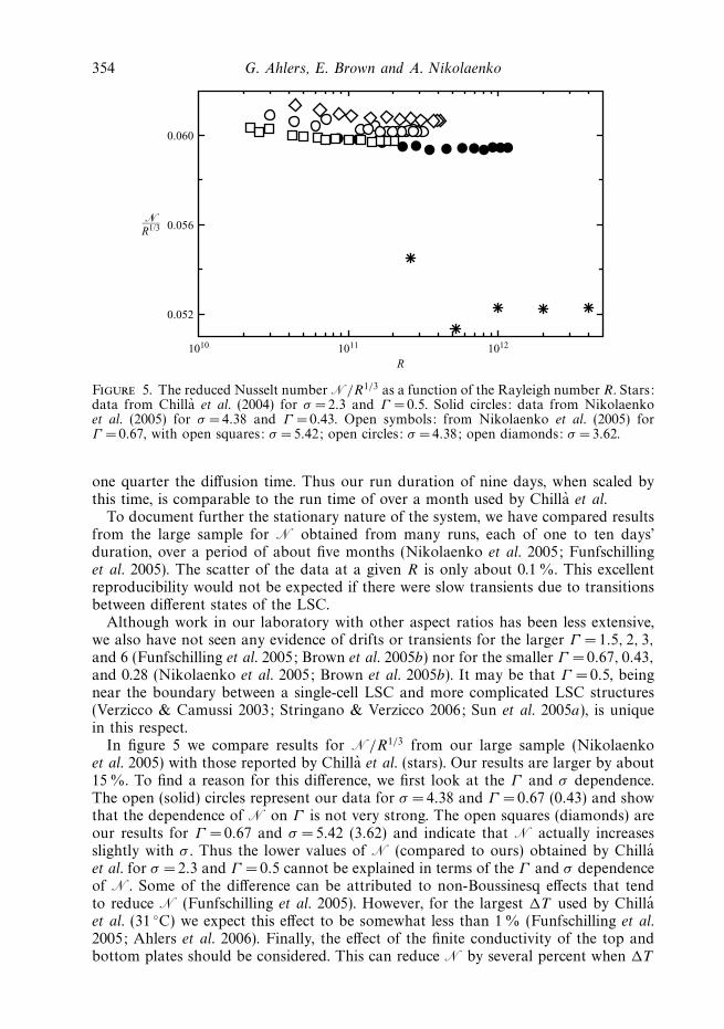
Figure 5. The reduced Nusselt number N/R1/3 as a function of the Rayleigh number R. Stars:data from Chilla et al. (2004) for σ = 2.3 and Γ = 0.5. Solid circles: data from Nikolaenkoet al. (2005) for σ = 4.38 and Γ = 0.43. Open symbols: from Nikolaenko et al. (2005) forΓ = 0.67, with open squares: σ =5.42; open circles: σ = 4.38; open diamonds: σ =3.62.

one quarter the diffusion time. Thus our run duration of nine days, when scaled bythis time, is comparable to the run time of over a month used by Chilla et al.

To document further the stationary nature of the system, we have compared resultsfrom the large sample for N obtained from many runs, each of one to ten days’duration, over a period of about five months (Nikolaenko et al. 2005; Funfschillinget al. 2005). The scatter of the data at a given R is only about 0.1 %. This excellentreproducibility would not be expected if there were slow transients due to transitionsbetween different states of the LSC.

Although work in our laboratory with other aspect ratios has been less extensive,we also have not seen any evidence of drifts or transients for the larger Γ = 1.5, 2, 3,

and 6 (Funfschilling et al. 2005; Brown et al. 2005b) nor for the smaller Γ =0.67, 0.43,

and 0.28 (Nikolaenko et al. 2005; Brown et al. 2005b). It may be that Γ = 0.5, beingnear the boundary between a single-cell LSC and more complicated LSC structures(Verzicco & Camussi 2003; Stringano & Verzicco 2006; Sun et al. 2005a), is uniquein this respect.

In figure 5 we compare results for N/R1/3 from our large sample (Nikolaenkoet al. 2005) with those reported by Chilla et al. (stars). Our results are larger by about15 %. To find a reason for this difference, we first look at the Γ and σ dependence.The open (solid) circles represent our data for σ =4.38 and Γ = 0.67 (0.43) and showthat the dependence of N on Γ is not very strong. The open squares (diamonds) areour results for Γ = 0.67 and σ =5.42 (3.62) and indicate that N actually increasesslightly with σ . Thus the lower values of N (compared to ours) obtained by Chillaet al. for σ =2.3 and Γ = 0.5 cannot be explained in terms of the Γ and σ dependenceof N. Some of the difference can be attributed to non-Boussinesq effects that tendto reduce N (Funfschilling et al. 2005). However, for the largest �T used by Chillaet al. (31 ◦C) we expect this effect to be somewhat less than 1 % (Funfschilling et al.2005; Ahlers et al. 2006). Finally, the effect of the finite conductivity of the top andbottom plates should be considered. This can reduce N by several percent when �T

The search for slow transients in turbulent Rayleigh–Benard convection 355

0 40 80 120 1600.992

0.996

1.000

1.004

Time (h)

�(β)——–�(0)

Figure 6. The reduced Nusselt number N(β)/N(0) as a function of time for the large sampleand R = 9.43 × 1010. Open circles: tilt angle β =0. Solid circles: β = 0.087 rad. Open squares:β = 0.122 rad. All data are normalized by the average N(0) of the data for β = 0. Each datapoint is based on temperature and heat-current measurements over a 2 h period. The verticaldotted lines indicate the times when β was changed.

is large (Chaumat, Castaing & Chilla 2002; Verzicco 2004; Brown et al. 2005b), but itis difficult to say precisely by how much. It seems unlikely that this effect can explainthe entire difference, particularly at the smaller R (and thus �T ) where it is relativelysmall.

4. Tilt-angle dependence of the Nusselt numberIn figure 6 we show results for N from the large sample at R = 9.43 × 1010.

Each data point was obtained from a 2 h average of measurements of the varioustemperatures and of Q. Three data sets, taken in temporal succession, for tilt anglesβ = 0, 0.087, and 0.122 rad are shown. All data were normalized by the mean of theresults for β =0. Typically, the standard deviation from the mean of the data at agiven β was 0.13 %. The vertical dotted lines and the change in the data symbolsshow where β was changed. Tilting the cell caused a small but measurable reductionon N. In figure 7 we show the mean value for each tilt angle, obtained from runs ofat least a day’s duration at each β , as a function of |β|. N decreases linearly with β .A fit of a straight line to the data yielded

N(β) = N0[1 − (3.1 ± 0.1) × 10−2|β|], (4.1)

with N0 = 273.5. Simlar results for the medium cell are compared with the large-cellresults in figure 8. At the smaller Rayleigh number of the medium sample the effectof β on N is somewhat less. Because the effect of β on N is so small, we did notmake a more detailed investigation of its Rayleigh-number dependence.

Chilla et al. proposed a model that predicts a significant tilt-angle effect on N forΓ = 0.5 where they assume the existence of two LSC cells, one above the other. Theyalso assumed that there would be no effect for Γ = 1 where there is only one LSC

356 G. Ahlers, E. Brown and A. Nikolaenko

0 0.04 0.08 0.12272.5

273.0

273.5

|β|

Nus

selt

num

ber

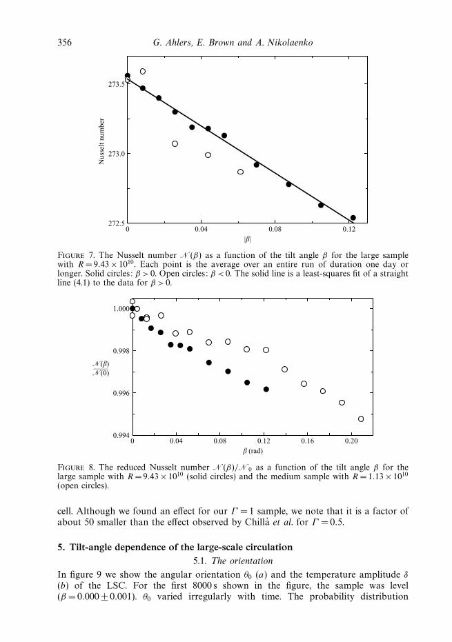
Figure 7. The Nusselt number N(β) as a function of the tilt angle β for the large samplewith R = 9.43 × 1010. Each point is the average over an entire run of duration one day orlonger. Solid circles: β > 0. Open circles: β < 0. The solid line is a least-squares fit of a straightline (4.1) to the data for β > 0.

0 0.04 0.08 0.12 0.16 0.200.994

0.996

0.998

1.000

β (rad)

�(β)——� (0)

Figure 8. The reduced Nusselt number N(β)/N0 as a function of the tilt angle β for thelarge sample with R = 9.43 × 1010 (solid circles) and the medium sample with R = 1.13 × 1010

(open circles).

cell. Although we found an effect for our Γ = 1 sample, we note that it is a factor ofabout 50 smaller than the effect observed by Chilla et al. for Γ =0.5.

5. Tilt-angle dependence of the large-scale circulation5.1. The orientation

In figure 9 we show the angular orientation θ0 (a) and the temperature amplitude δ

(b) of the LSC. For the first 8000 s shown in the figure, the sample was level(β =0.000 ± 0.001). θ0 varied irregularly with time. The probability distribution

The search for slow transients in turbulent Rayleigh–Benard convection 357

0

0.4

0.8

Time (s)

θ0—2π

1 × 104 2 × 1040

0.2δ (K)

(a)

(b)

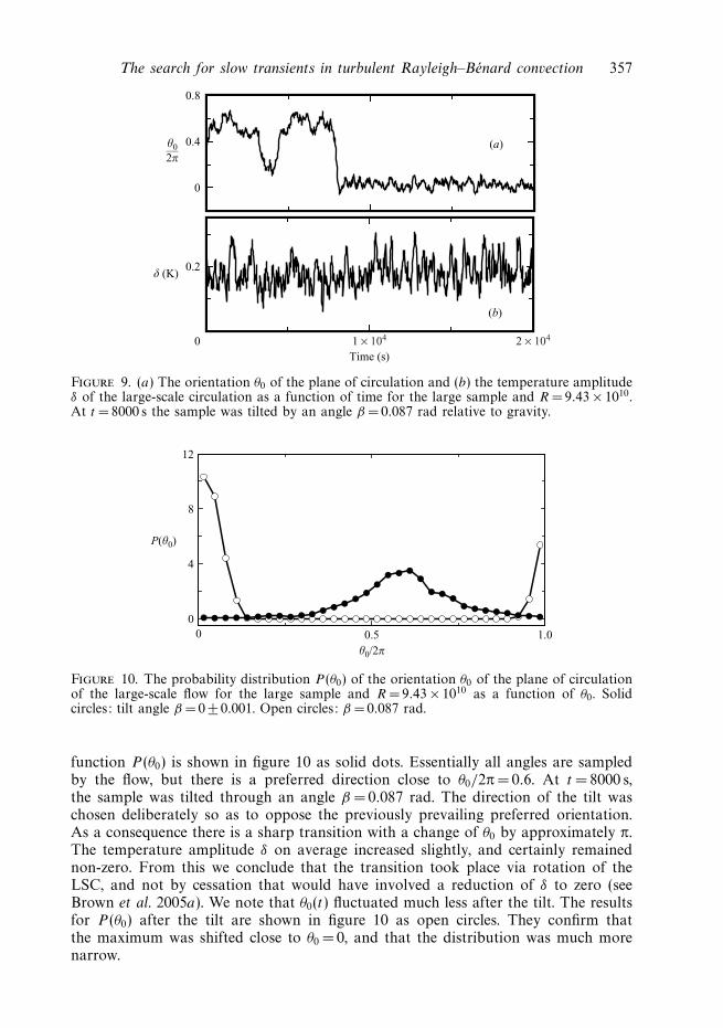
Figure 9. (a) The orientation θ0 of the plane of circulation and (b) the temperature amplitudeδ of the large-scale circulation as a function of time for the large sample and R = 9.43 × 1010.At t = 8000 s the sample was tilted by an angle β =0.087 rad relative to gravity.

0.5 1.00

0

4

8

12

θ0/2π

P(θ0)

Figure 10. The probability distribution P (θ0) of the orientation θ0 of the plane of circulationof the large-scale flow for the large sample and R = 9.43 × 1010 as a function of θ0. Solidcircles: tilt angle β = 0 ± 0.001. Open circles: β = 0.087 rad.

function P (θ0) is shown in figure 10 as solid dots. Essentially all angles are sampledby the flow, but there is a preferred direction close to θ0/2π = 0.6. At t = 8000 s,the sample was tilted through an angle β = 0.087 rad. The direction of the tilt waschosen deliberately so as to oppose the previously prevailing preferred orientation.As a consequence there is a sharp transition with a change of θ0 by approximately π.The temperature amplitude δ on average increased slightly, and certainly remainednon-zero. From this we conclude that the transition took place via rotation of theLSC, and not by cessation that would have involved a reduction of δ to zero (seeBrown et al. 2005a). We note that θ0(t) fluctuated much less after the tilt. The resultsfor P (θ0) after the tilt are shown in figure 10 as open circles. They confirm thatthe maximum was shifted close to θ0 = 0, and that the distribution was much morenarrow.

358 G. Ahlers, E. Brown and A. Nikolaenko

–0.2 0 0.20

4

8

12

θ0 (rad)

P(θ0)

Figure 11. The probability distribution P (θ0) of the orientation θ0 of the plane of circulationof the large-scale flow for the large sample and R = 9.43 × 1010 at three tilt angles β . Solidcircles: β = 0.122 rad. Open circles: β = 0.044 rad. Solid squares: β = 0.026 rad.

–0.05 0 0.05 0.10

10–1

β (rad)

σθ (rad)

Figure 12. The square root of the variance σθ of the probability distribution P (θ0) of theorientation θ0 of the plane of circulation of the large-scale flow for the large sample andR = 9.43 × 1010 as a function of the tilt angle β .

In figure 11 we show P (θ0) for β = 0.122 (solid circles), 0.044 (open circles), and0.026 (solid squares). A reduction of β leads to a broadening of P (θ0). The square rootof the variance of data like those in figure 11 is shown in figure 12 on a logarithmicscale as a function of β on a linear scale. Even a rather small tilt angle caused severenarrowing of P (θ0).

5.2. The temperature amplitude

In figure 13 we show the temperature amplitude δ(β) of the LSC as a function ofβ . As was the case for N, the data are averages over the duration of a run at agiven β (typically a day or two). The solid (open) circles are for positive (negative)β . The data can be represented well by either a linear or a quadratic equation. Aleast-squares fit yielded

δ(β) = δ(0) × [1 + (1.84 ± 0.45)|β| − (3.1 ± 3.9)β2] (5.1)

with δ(0) = 0.164 K.

The search for slow transients in turbulent Rayleigh–Benard convection 359

0 0.04 0.08 0.120.16

0.17

0.18

0.19

0.20

δ (K)

|β| (rad)

Figure 13. The time-averaged temperature amplitude δ(β) of the LSC for the large sampleas a function of |β|. Solid circles: β � 0. Open circles: β < 0. For this example R = 9.43 × 1010.

5.3. The Reynolds numbers

Using (2.2), we calculated the auto-correlation functions (AC) Ci,i, i = 0, . . . , 7, as wellas the cross-correlation functions (CC) Ci,j , j =[(i + 4) mod 8], i = 0, . . . , 7, of thetemperatures measured on opposite sides of the sample. Typical examples are shownin figure 14. The CC has a characteristic peak that we associate with the passage ofrelatively hot or cold volumes of fluid at the thermometer locations. Such temperaturecross-correlations have been shown, e.g. by Qiu & Tong (2001b, 2002), to yield delaytimes equal to those of velocity-correlation measurements, indicating that warm orcold fluid volumes travel with the LSC. The function

Ci,j (τ ) = −b0 exp

(− τ

τi,j

0

)− b1 exp

[−

(τ − t

i,j

1

τi,j

1

)2], (5.2)

consisting of an exponentially decaying background (that we associate with therandom time evolution of θ0) and a Gaussian peak, was fitted to the data for the CC.The fitted function is shown in figure 14 as a solid line over the range of τ used inthe fit. It is an excellent representation of the data and yields the half turnover timeT/2 = t

i,j

1 of the LSC. Similarly, we fitted the function

Ci,i(τ ) = b0 exp

(− τ

τ i,i0

)+ b1 exp

[−

(τ

τ i,i1

)2]+ b2 exp

[−

(τ − t i,i

2

τ i,i2

)2](5.3)

to the AC data. It consists of two Gaussian peaks, one centred at τ = 0 and theother at τ = t i,i

2 , and the exponential background. We interpret the location t i,i2 of the

second Gaussian peak as corresponding to a complete turnover time T of the LSC.In terms of the averages 〈t i,j

1 〉 and 〈t i,i2 〉 over all 8 thermometers or thermometer-pair

combinations we define (Qiu & Tong 2002; Grossmann & Lohse 2002) the Reynolds

360 G. Ahlers, E. Brown and A. Nikolaenko

0 50 100

1

τ (s)

–10

3 C04

and

103 C

00 (

°C)2

2

3

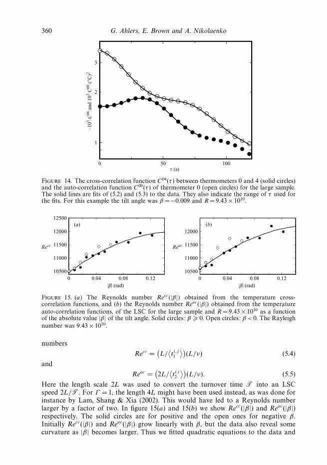
Figure 14. The cross-correlation function C04(τ ) between thermometers 0 and 4 (solid circles)and the auto-correlation function C00(τ ) of thermometer 0 (open circles) for the large sample.The solid lines are fits of (5.2) and (5.3) to the data. They also indicate the range of τ used forthe fits. For this example the tilt angle was β = −0.009 and R = 9.43 × 1010.

10500

11000

11500

12000

12500

|β| (rad)

Recc

0 0.04 0.08 0.12|β| (rad)

0 0.04 0.08 0.1210500

11000

11500

12000(a) (b)

Reac

Figure 15. (a) The Reynolds number Recc(|β|) obtained from the temperature cross-correlation functions, and (b) the Reynolds number Reac(|β|) obtained from the temperatureauto-correlation functions, of the LSC for the large sample and R = 9.43 × 1010 as a functionof the absolute value |β| of the tilt angle. Solid circles: β � 0. Open circles: β < 0. The Rayleighnumber was 9.43 × 1010.

numbers

Recc =(L/

⟨ti,j

1

⟩)(L/ν) (5.4)

and

Reac =(2L/

⟨t i,i2

⟩)(L/ν). (5.5)

Here the length scale 2L was used to convert the turnover time T into an LSCspeed 2L/T. For Γ = 1, the length 4L might have been used instead, as was done forinstance by Lam, Shang & Xia (2002). This would have led to a Reynolds numberlarger by a factor of two. In figure 15(a) and 15(b) we show Recc(|β|) and Reac(|β|)respectively. The solid circles are for positive and the open ones for negative β .Initially Recc(|β|) and Reac(|β|) grow linearly with β , but the data also reveal somecurvature as |β| becomes larger. Thus we fitted quadratic equations to the data and

The search for slow transients in turbulent Rayleigh–Benard convection 361

|β| (rad)

0 0.04 0.08 0.12

16000

17000

18000

19000

Reτ

Figure 16. The Reynolds number Reτ (|β|) obtained from the half-widths τ1 of the temperaturecross-correlation functions (solid circles) and from the half-widths τ1 (open squares) and τ2

(open circles) of the temperature auto-correlation functions as a function of the tilt angle. TheRayleigh number was 9.43 × 1010.

obtained

Recc(β) = Recc(0) × [1 + (1.85 ± 0.21)|β| − (5.9 ± 1.7)β2] (5.6)

and

Reac(β) = Reac(0) × [1 + (1.72 ± 0.38)|β| − (4.1 ± 3.2)β2] (5.7)

with Recc(0) = 10467 ± 43 and Reac(0) = 10565 ± 82 (all parameter errors are 67 %confidence limits). The results for Recc(0) and Reac(0) are about 10 % higher than theprediction by Grossmann & Lohse (2002) for our σ and R. The excellent agreementbetween Recc and Reac is consistent with the idea that the CC yields T/2 and that theAC gives T. As expected (see § 2), the β-dependences of both Reynolds numbers arethe same within their uncertainties. It is interesting to see that the coefficients of thelinear term also agree with the corresponding coefficient for δ (equation (5.1)). Thissuggests that there may be a closer relationship between δ and Re than we wouldhave expected a priori. However, the coefficient of the linear term in (5.6) or (5.7)is larger by a factor of about 50 than the corresponding coefficient for the Nusseltnumber in (4.1).

Although the precise meaning of the half-widths τ1 and τ2 in (5.2) and (5.3) isless clear than that of t1 and t2, it is of some interest to compute the correspondingReynolds numbers Reτ from (5.4). These are shown in figure 16. They are about 40 %larger than Reac or Recc, and all three are of about the same size. The results obtainedfrom the AC show considerable scatter, and the β-dependence is not resolved very well.On the other hand, the result from the half-width of the Gaussian peak of the CC ismore precise, and a fit of a straight line to the data yields Reτ =Reτ (0) × (1 + 2.27|β|)with Reτ (0) = 15130.

In figure 17 we show measurements of Recc and of δ, each normalized by its valueat β =0, as a function of β for the medium sample and R =1.13 × 1010. For thissample we were able to attain larger values of β than for the large one. It is seen thatδ and Recc have about the same β dependence for small β , but that δ then increasesmore rapidly than Recc as β becomes large. Although we do not know the reasonfor this behaviour, it suggests that the larger speed of the LSC enhances the thermalcontact between the sidewall and the fluid interior.

362 G. Ahlers, E. Brown and A. Nikolaenko

0 0.1 0.2

1.0

1.2

1.4

1.6

1.8

β (rad)

Recc

(β)/

Recc

(0),

δ(β

)/δ(0

)

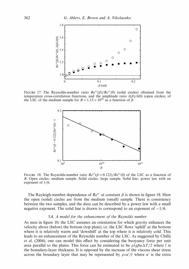
Figure 17. The Reynolds-number ratio Recc(β)/Recc(0) (solid circles) obtained from thetemperature cross-correlation functions, and the amplitude ratio δ(β)/δ(0) (open circles), ofthe LSC of the medium sample for R = 1.13 × 1010 as a function of β .

109 1010 10110.1

0.3

R

Recc

(β =

0.1

22)/

Recc

(0)

–1

Figure 18. The Reynolds-number ratio Recc(β = 0.122)/Recc(0) of the LSC as a function ofR. Open circles: medium sample. Solid circles: large sample. Solid line: power law with anexponent of 1/6.

The Rayleigh-number dependence of Recc at constant β is shown in figure 18. Herethe open (solid) circles are from the medium (small) sample. There is consistencybetween the two samples, and the data can be described by a power law with a smallnegative exponent. The solid line is drawn to correspond to an exponent of −1/6.

5.4. A model for the enhancement of the Reynolds number

As seen in figure 10, the LSC assumes an orientation for which gravity enhances thevelocity above (below) the bottom (top plate), i.e. the LSC flows ‘uphill’ at the bottomwhere it is relatively warm and ‘downhill’ at the top where it is relatively cold. Thisleads to an enhancement of the Reynolds number of the LSC. As suggested by Chillaet al. (2004), one can model this effect by considering the buoyancy force per unitarea parallel to the plates. This force can be estimated to be ρlgβα�T/2 where l isthe boundary-layer thickness. It is opposed by the increase of the viscous shear stressacross the boundary layer that may be represented by ρνu′/l where u′ is the extra

The search for slow transients in turbulent Rayleigh–Benard convection 363

speed gained by the LSC due to the tilt. Equating the two, substituting

l = L/(2N), (5.8)

solving for u′, using (1.2) for R, and defining Re′ ≡ (L/ν)u′ one obtains

Re′ =Rβ

8σN2(5.9)

for the enhancement of the Reynolds number of the LSC. From our measurements atlarge R we found that Re and N (Nikolaenko et al. 2005) can be represented withinexperimental uncertainty by

Re = 0.0345R1/2, (5.10)

N = 0.0602R1/3, (5.11)

giving

Re ′

Re= 1.00 × 103R−1/6σ −1β. (5.12)

For our σ =4.38 and R = 9.43 × 1010 one finds Re′/Re = 3.4β , compared to theexperimental value (1.9 ± 0.2)β from Recc (equation (5.6)) and (1.7 ± 0.4)β from Reac

(equation (5.7)). We note that the coefficient 1.00 × 103 in (5.12) depends on thedefinition of Re given in (5.4) and (5.5) that was used in deriving the result (5.10).If the length scale 4L had been used instead of 2L to define the speed of the LSC,as was done for instance by Lam et al. (2002), this coefficient would have beensmaller by a factor of two, yielding near-perfect agreement with the measurements.In figure 18 the predicted dependence on R−1/6 also is in excellent agreement with theexperimental results. However, such good agreement may be somewhat fortuitous,considering the approximations that were made in the model. Particularly the use of(5.8) for the boundary-layer thickness is called into question at a quantitative level bymeasurements of Lui & Xia (1998) that revealed a significant variation of l with lateralposition. In addition, it is not obvious that the thermal boundary-layer thickness lshould be used, as suggested by Chilla et al. (2004), to estimate the shear stress;perhaps the thickness of the viscous boundary layer would be more appropriate.

In discussing their Γ = 0.5 sample, Chilla et al. (2004) took the additional step ofassuming that the relative change of N due to a finite β is equal to the relativechange of Re. For our sample with Γ =1 this assumption does not hold. As we sawabove, the relative change of N is a factor of about 50 less than the relative changeof Re. The origin of the (small) reduction of the Nusselt number is not obvious.Naively one might replace g in the definition of the Rayleigh number by g cos(β);but this would lead to a correction of order β2 whereas the experiment shows thatthe correction is of order β , albeit with a coefficient that is smaller than of order one.The linear dependence suggests that the effect of β on N may be provoked by thechange of Re with β , but not in a direct causal relationship.

6. Tilt-angle dependence of reorientations of the large-scale circulationIt is known from direct numerical simulation (Hansen, Yuen & Kroening 1991) and

from several experiments (Cioni, Ciliberto & Sommeria 1997; Niemela et al. 2001;Sreenivasan et al. 2002; Brown et al. 2005a) that the LSC can undergo relativelysudden reorientations. Not unexpectedly, we find that the tilt angle strongly influencesthe frequency of such events. For a level sample (β =0) we demonstrated elsewhere(Brown et al. 2005a) that reorientations can involve changes of the orientation of the

364 G. Ahlers, E. Brown and A. Nikolaenko

–0.05 0 0.05 0.100

0.5

1.0

1.5

β (rad)

Reo

rien

tati

ons/

h

Figure 19. The number of reorientation events per hour of the angular orientation of the planeof circulation of the LSC in the large sample for R = 9.43 × 1010. The solid line shows (6.1).

plane of circulation of the LSC through any angular increment �θ , with the probab-ility P (�θ) increasing with decreasing �θ . Thus, in order to define a ‘reorientation’,we established certain criteria. We required that the magnitude of the net angularchange |�θ | had to be greater than �θmin = (2π)/8. In addition we specified that themagnitude of the net average azimuthal rotation rate |θ | ≡ |�θ/�t | had to be greaterthan θmin =0.1/T where T is the LSC turnover time and �t is the duration of thereorientation (we refer to Brown et al. (2005a) for further details). Using these criteria,we found that the number of reorientation events n(β) at constant R = 9.43 × 1010

decreased rapidly with increasing |β|. These results are shown in figure 19. It is worthnoting that nearly all of these events are rotations of the LSC and very few involveda cessation of the circulation. A least-squares fit of the Gaussian function

n(β) = N0 exp[−(β − β0)2/w2] (6.1)

to the data yielded N0 = 1.23 ± 0.06 events per hour, β0 = 0.0093 ± 0.0010 rad, andw = 0.0251 ± 0.0015 rad. It is shown by the solid line in the figure.

We note that the distribution function is not centred on β = 0. The displacement ofthe centre by about 9 mrad is much more than the probable error of β . We believethat it is caused by the effect of the Coriolis force on the LSC that will be discussedin more detail elsewhere (Brown & Ahlers 2006).

7. Tilt-angle dependence of the centre temperatureWe saw from figure 13 that the increase of Re with β led to an increase of the

amplitude δ of the azimuthal temperature variation at the horizontal mid-plane. Anadditional question is whether the tilt-angle effect on this system has an asymmetrybetween the top and bottom that would lead to a change of the mean centretemperature Tc (see (2.1)). Chilla et al. (2004) report such an effect for their Γ = 0.5sample. For a Boussinesq sample with β = 0 we expect that Tc = Tm with Tm = (Tt +Tb)/2 (Tt and Tb are the top and bottom temperatures respectively), or equivalentlythat �t = Tc − Tt is equal to �b = Tb − Tc. A difference between �b and �t willoccur when the fluid properties have a significant temperature dependence (Wu &Libchaber 1991; Zhang, Childress & Libchaber 1997; Ahlers et al. 2006), i.e. whenthere are significant deviations from the Boussinesq approximation. For the sequenceof measurements with the large apparatus and R = 9.43 × 1010, as a function of β the

The search for slow transients in turbulent Rayleigh–Benard convection 365

β (rad)

(Tc

– T

m)

(K)

0 0.05 0.10

0.48

0.49

9.5

10.0

10.5

∆t

and

∆b

(K

)

(a)

(b)

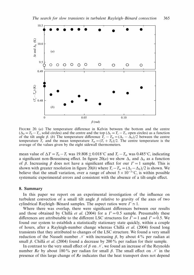
Figure 20. (a) The temperature difference in Kelvin between the bottom and the centre(�b = Tb −Tc , solid circles) and the centre and the top (�t = Tc −Tt , open circles) as a functionof the tilt angle β . (b) The temperature difference Tc − Tm = (�t − �b)/2 between the centretemperature Tc and the mean temperature Tm = (Tt + Tb)/2. The centre temperature is theaverage of the values given by the eight sidewall thermometers.

mean value of �T = Tb −Tt was 19.808 ± 0.018◦C and Tc −Tm was 0.485◦C, indicatinga significant non-Boussinesq effect. In figure 20(a) we show �t and �b as a functionof β . Increasing β does not have a significant effect for our Γ = 1 sample. This isshown with greater resolution in figure 20(b) where Tc −Tm = (�t −�b)/2 is shown. Webelieve that the small variation, over a range of about 5 × 10−3◦C, is within possiblesystematic experimental errors and consistent with the absence of a tilt-angle effect.

8. SummaryIn this paper we report on an experimental investigation of the influence on

turbulent convection of a small tilt angle β relative to gravity of the axes of twocylindrical Rayleigh–Benard samples. The aspect ratios were Γ � 1.

Where there was overlap, there were significant differences between our resultsand those obtained by Chilla et al. (2004) for a Γ = 0.5 sample. Presumably thesedifferences are attributable to the different LSC structures for Γ = 1 and Γ = 0.5. Wefound our system to establish a statistically stationary state quickly, within a coupleof hours, after a Rayleigh-number change whereas Chilla et al. (2004) found longtransients that they attributed to changes of the LSC structure. We found a very smallreduction of the Nusselt number N with increasing β , by about 4% per radian atsmall β . Chilla et al. (2004) found a decrease by 200 % per radian for their sample.

In contrast to the very small effect of β on N, we found an increase of the Reynoldsnumber Re by about 180 % per radian for small β . The small effect on N in thepresence of this large change of Re indicates that the heat transport does not depend

366 G. Ahlers, E. Brown and A. Nikolaenko

strongly on the speed of the LSC sweeping over the boundary layers. Instead, N mustbe determined by instability mechanisms of the boundary layers, and the associatedefficiency of the ejection of hot (cold) volumes (so-called ‘plumes’) of fluid from thebottom (top) boundary layer.

It is interesting to note that the strong dependence of Re on β in the presence ofonly a very weak dependence of N on β can be accommodated quite well withinthe model of Grossmann & Lohse (2002). The Reynolds number can be changed byintroducing a β-dependence of the parameter a(β) in their equations (4) and (6). Aspointed out by them, a change of a has no influence on the predicted value for N.

We also measured the frequency of rapid LSC reorientations that are known tooccur for β =0. We found that such events are strongly suppressed by a finite β . Evena mild breaking of the rotational invariance, corresponding to β � 0.04, suppressesre-orientations almost completely.

We are grateful to Siegfried Grossmann and Detlef Lohse for fruitful exchanges.This work was supported by the United States Department of Energy through GrantDE-FG02-03ER46080.

REFERENCES

Ahlers, G., Brown, E., Fontenele Araujo, F., Funfschilling, D., Grossmann, S. & Lohse, D.

2006 Non-Oberbeck-Boussinesq effects in strongly turbulent Rayleigh–Benard convection. J.Fluid Mech., submitted.

Ahlers, G., Grossmann, S. & Lohse, D. 2002 Hochprazision im Kochtopf: Neues zur turbulentenKonvektion. Physik J. 1(2), 31–37.

Belmonte, A., Tilgner, A. & Libchaber, A. 1995 Turbulence and internal waves in side-heatedconvection. Phys. Rev. E 51, 5681–5687.

Brown, E. & Ahlers, G. 2006 Effect of Earth’s Coriolis force on the large-scale circulation inturbulent Rayleigh-Benard convection in the laboratory. J. Fluid Mech. (submitted)

Brown, E., Nikolaenko, A. & Ahlers, G. 2005a Orientation changes of the large-scale circulationin turbulent Rayleigh-Benard convection. Phys. Rev. Lett. 95, 084503-1–4.

Brown, E., Nikolaenko, A., Funfschilling, D. & Ahlers, G. 2005b Heat transport in turbulentRayleigh–Benard convection: Effect of finite top- and bottom-plate conductivity. Phys. Fluids17, 075108.

Castaing, B., G. Gunaratne, G., Heslot, F., Kadanoff, L., Libchaber, L., Thomae, S., Wu, X.-Z.,

Zaleski, S. & Zanetti, G. 1989 Scaling of hard thermal turbulence in Rayleigh–Benardconvection. J. Fluid Mech. 204, 1–30.

Chaumat, S., Castaing, B. & Chilla, F. 2002 Rayleigh–Benard cells: influence of the plates prop-erties Advances in Turbulence IX, Proc. Ninth European Turbulence Conf. (ed. I. P. Castro &P. E. Hancock). CIMNE, Barcelona.

Chilla, F., Rastello, M., Chaumat, S. & Castaing, B. 2004 Long relaxation times and tiltsensitivity in Rayleigh–Benard turbulence. Eur. Phys. J. B 40, 223–227.

Ciliberto, S., Cioni, S. & Laroche, C. 1996 Large-scale flow properties of turbulent thermalconvection. Phys. Rev. E 54, R5901–R5904.

Cioni, S., Ciliberto, S. & Sommeria, J. 1997 Strongly turblent Rayleigh–Benard convection inmercury: comparison with results at moderate Prandtl number. J. Fluid Mech. 335, 111–140.

Funfschilling, D., Brown, E., Nikolaenko, A. & Ahlers, G. 2005 Heat transport by turbulentRayleigh–Benard Convection in cylindrical samples with aspect ratio one and larger. J. FluidMech. 536, 145–154.

Grossmann, S. & Lohse, D. 2001 Thermal convection for large Prandtl number. Phys. Rev. Lett.86, 3317–3319.

Grossmann, S. & Lohse, D. 2002 Prandtl and Rayleigh number dependence of the Reynoldsnumber in turbulent thermal convection. Phys. Rev. E 66, 016305, 1–6.

The search for slow transients in turbulent Rayleigh–Benard convection 367

Hansen, U., Yuen, D. A. & Kroening, S. E. 1991 Mass and heat transport in strongly time-dependent thermal convection at infinite Prandtl number. Geophys. Astrophys. Fluid Dyn. 63,67–89.

Kadanoff, L. P. 2001 Turbulent heat flow: Structures and scaling. Phys. Today 54 (8), 34–39.

Kraichnan, R. 1962 Turbulent thermal convection at arbitrary Prandtl number. Phys. Fluids 5,1374–1389.

Krishnamurty, R. & Howard, L. N. 1981 Large-scale flow generation in turbulent convection.Proc. Natl Acad. Sci. USA 78, 1981–1985.

Lam, S., Shang, X.-D. & Xia, K.-Q. 2002 Prandtl number dependence of the viscous boundary layerand the Reynolds numbers in Rayleigh–Benard convection. Phys. Rev. E 65, 066306 1–8.

Lui, S.-L. & Xia, K.-Q.1998 Spatial structure of the thermal boundary layer in turbulent convection.Phys. Rev. E 57, 5494–5503.

Niemela, J., Skrbek, L., Sreenivasan, K. & Donnelly, R. 2001 The wind in confined thermalConvection. J. Fluid Mech. 449, 169–178.

Nikolaenko, A., Brown, E., Funfschilling, D. & Ahlers, G. 2005 Heat transport by turbulentRayleigh–Benard Convection in cylindrical cells with aspect ratio one and less. J. Fluid Mech.523, 251–260.

Qiu, X.-L. & Tong, P. 2001a Large-scale velocity structures in turbulent thermal convection. Phys.Rev. E 64, 036304, 1–13.

Qiu, X.-L. & Tong, P. 2001b Onset of coherent oscillations in turbulent Rayleigh–Benard convection.Phys. Rev. Lett. 87, 094501, 1–4.

Qiu, X.-L. & Tong, P. 2002 Temperature oscillations in turbulent Rayleigh–Benard convection.Phys. Rev. E 66, 026208, 1–11.

Roche, P.-E., Castaing, B., Chabaud, B. & Hebral, B. 2004 Heat transfer in turbulent Rayleigh–Benard convection below the ultimate regime. J. Low Temp. Phys. 134, 1011–1042.

Shraiman, B. I. & Siggia, E. D. 1990 Heat transport in high-Rayleigh number convection. Phys.Rev. A 42, 3650–3653.

Siggia, E. D. 1994 High Rayleigh number convection. Annu. Rev. Fluid Mech. 26, 137–168.

Sreenivasan, K., Bershadskii, A. & Niemela, J. 2002 Mean wind and its reversal in thermalconvection. Phys. Rev. E 65, 056306, 1–11.

Stringano, G. & Verzicco, R. 2006 Mean flow structure in thermal convection in a cylindrical cellof aspect-ratio one half. J. Fluid Mech. 548, 1–16.

Sun, C., Xi, H.-D. & Xia, K.-Q. 2005a Azimuthal symmetry, flow dynamics, and heat flux inturbulent thermal convection in a cylinder with aspect ratio one-half. Phys. Rev. Lett 95,074502-1–4.

Sun, C., Xia, K.-Q. & Tong, P. 2005b Three-dimensional flow structures and dynamics of turbulentthermal convection in a cylindrical cell. Phys. Rev. E 72, 026302, 1–13.

Verzicco, R. 2004 Effects of non-perfect thermal sources in turbulent thermal convection. Phys.Fluids 16, 1965–1979.

Verzicco, R. & Camussi, R. 2003 Numerical experiments on strongly turbulent thermal convectionin a slender cylindrical cell. J. Fluid Mech. 477, 19–49.

Wu, X.-Z. & Libchaber, A. 1991 Non-Boussinesq effects in free thermal convection. Phys. Rev. A43, 2833–2839.

Xi, H.-D., Lam, S. & Xia, K.-Q. 2004 From laminar plumes to organized flows: the onset oflarge-scale circulation in turbulent thermal convection. J. Fluid Mech. 503, 47–56.

Zhang, J., Childress, S. & Libchaber, A. 1997 Non-Boussinesq effect: Thermal convection withbroken symmetry. Phys. Fluids 9, 1034–1042.