Stress evolution during Volmer-Weber thin film growth: a multi-scale approach for modeling diffusion, cohesion and attachment. by Juan S Tello B.S. Aerospace Engineering, Boston University, 2002 Sc.M. Mechanical Engineering, Brown University, 2007 A dissertation presented in partial fulfillment of the requirements for the degree of Doctor of Philosophy at Brown University in the subject of Mechanics of Solids and Structures Brown University Providence, Rhode Island May 2008
Transcript
Stress evolution during Volmer-Weber thin film growth:a multi-scale approach for modeling diffusion, cohesion
and attachment.
by
Juan S Tello
B.S. Aerospace Engineering, Boston University, 2002
Sc.M. Mechanical Engineering, Brown University, 2007
Thin film technology, which has been around for several decades, underwent dramatic
advances over the 1990’s and early 2000’s. Many current technologies rely on the creative
application of thin film materials and structures, and this is likely to continue through the
near and distant futures. Below is a list of some recent technological developments which rely
on thin film technology:
• Holographic storage, which has recently become commercially available, has increased
the amount of data that can be contained in a CD-sized disk to about 600 GB. This
remarkable achievement has been made possible in part by enhanced understanding and
application of thin film deposition and processing methods.
• Thin film technology also promises to facilitate the development solar panels that will
be more reliable, efficient and cost effective than their modern counterparts. Several
joint operations between industry and government have been recently initiated, such
as General Electric’s venture with a U.S. federal program to make solar power cost
competitive by 2015 [1].
• Thin film technology will also play a key role in the development of more efficient en-
ergy storage, such as solid-state micro-batteries, which will feature longer operational
1
Chapter 1: Introduction and background 2
lifetimes, increased safety and a less damaging environmental impact than existing bat-
tery technologies.
• Thin films have recently been used to create miniature thermoelectric coolers and heaters
by Nextreme, a thin film manufacturing firm. The new devices feature high-power
densities and microsecond response times inside a volume of about 0.3mm x 0.3mm x
0.1mm. Sensors such as this will dramatically improve cooling and heating systems in
electronic applications by providing fast response times and highly localized thermal
control.
• Thin films will also be instrumental in the development of flexible displays for future ‘e-
paper’ which consists of transparent transistors that can change their optical properties
in a controlled fashion and function by reflecting light instead of emitting it. This can
dramatically improve the energy efficiency and flexibility of future displays.
• A novel application of thin film technology in retinal implants, such as that under devel-
opment by a team lead by Professor Eberhart Zrenner at the University Eye Hospital in
Tbingen, Germany, promises to restore sight to patients suffering from a disease which
damages the light sensing neurons in the human retina. As of 2007 the existing implants,
which are similar to the CMOS sensors found in digital cameras, contain too few tran-
sistors, and hence produce very coarse images. The successful implementation of these
implants, as of many other digital imaging technologies, will depend on the development
of sensors with extremely high transistor densities. Such requirements will only be met
with improved methods of thin film manufacturing and design as challenges continue to
emerge at the ever shrinking length scales.
This list elucidates the momentous importance that thin films will play in future technologies,
and highlights the need for better understanding of thin film material behavior and processing
methods.
Chapter 1: Introduction and background 3
One of the most prominent challenges facing researches today lies in controlling internal
stresses in thin film systems, both during and after the manufacturing process. Thin solid films
often exhibit large stresses which are ‘grown in’ as the material is deposited onto a substrate.
These stresses may arise as a result of many physical, chemical and even biological processes.
Some common causes of internal stresses in thin films include (i) mismatch strains between
adjacent layers of materials, (ii) kinetic processes involving diffusion into grain boundaries,
thermal expansion coefficient mismatch across interfaces, among others. The consequences of
high film stresses are almost always undesirable, and range from inducing considerable curva-
tures on the substrates holding the film, to permanent deformation of the film or substrate,
to film cracking and delamination.
This dissertation presents a model of stress generation in polycrystalline thin films during
the deposition of film material onto a flat substrate. The model considers a type of thin
film growth process known as Volmer-Weber (VM) growth. Chapter 2 contains an exten-
sive review of experimental observations of stress evolution during VM growth and outlines
the most relevant existing models which have attempted to estimate the magnitude of these
stresses. It proceeds to describe the model system, derive its governing equations and their
implementation in a finite element code. In Chapter 3 the model is thoroughly analyzed by
means of dimensional analysis and several parameter studies and its predictions are compared
with several experimental observations.
Finally, Chapter 4 describes a method for coupling discrete and continuum descriptions of
the same diffusive process. This methodology could serve as a means to facilitate the modeling
of triple junctions with a detailed kinetic Monte Carlo framework while treating the rest of the
islands with finite elements, which would save significant computational time. As presented
the formulation can handle simple linear diffusion, without stress gradients or specific site
energetics and this extension is not trivial. However it includes an efficient iterative boundary
condition application, and an automatic convergence criterion which make the method robust
Chapter 1: Introduction and background 4
and relatively fast.
Chapter 2
Modeling Volmer-Weber growth
Polycrystalline thin films are among the most studied types of thin film systems, partly
because of the wide range of technological applications that rely on them. Among these are
magnetic storage media, thermal barrier coatings, piezoelectric sensors and actuators, among
others. The successful performance of these films depends critically on the ability to control
and faithfully reproduce the manufacturing process. Consequently, understanding the effects
of growth conditions and material properties on the resulting film characteristics is of crucial
importance to the continuing advancement of this field.
A characteristic feature of polycrystalline films is that, upon deposition of film material
onto a substrate, atoms of the film material bond more strongly with one another than they
do with the substrate. As a result, these atoms gather into clusters instead of wetting the
substrate uniformly. With further deposition, these clusters continue to grow and eventually
coalesce to form a continuous film.
During this process, called Volmer-Weber growth, polycrystalline films develop internal
stresses that vary significantly over the course of deposition. The stresses can be determined
experimentally by measuring the curvature κ of the substrate, which is related to the stress
5
Chapter 2: Modeling Volmer-Weber growth 6
in the film by means of the Stoney formula [29]
f =1
6κMshs (2.1)
where the ‘film force’ f is the resultant force per unit film thickness, and hs and Ms are the
substrate thickness and biaxial modulus, respectively. Experimental observations are often
reported in terms of f , or the ‘instantaneous stress’, σins, given by
σins =∂f
∂h(2.2)
where h is the volume-equivalent film thickness.
Film thickness, (arbitrary units)
Fil
m f
orc
e,
(ar
bit
rary
un
its)
f
h
0
(a)
(b)
(c)σins <0σins σins
ss=
increasing growth flux
Figure 2.1: Schematic of typical experimental observations during Volmber-Weber growth ofthin films.
Most experimental observations share the following features. During the early stages of
growth, when the films are in the form of isolated islands (Fig. 2.1(a)), the film force tends
to have a small compressive value. Then, as islands begin to coalesce (Fig. 2.1(b)), σins
increases rapidly, reaching a peak value when the film becomes continuous. Subsequently, a
quasi steady-state is attained (Fig. 2.1(c)) in which σins reaches a constant value, σssins, which
depends on deposition conditions and material properties. Nearly all experiments [26, 6, 13]
report compressive stresses after coalescence at low growth rates. Increasing the growth rate
Chapter 2: Modeling Volmer-Weber growth 7
tends to decrease the magnitude of steady-state compression, and may induce tension at very
high rates. In addition, materials with low surface diffusivities, such as ceramics, tend to
exhibit more tensile stresses than say, fcc metals, which have much higher surface and grain
boundary diffusivities at typical growth temperatures [26, 13].
The origin of the small compressive stress exhibited by films before they become fully con-
tinuous remains a controversial issue, and several different explanations have been proposed.
Camamrata et al [3] explain it in terms of surface stress effects; Friesen and Thompson [9]
have suggested that adatoms moving around the substrate and film surfaces act as effective
force dipoles inducing a compressive stress. However, the extent to which these mechanisms
are responsible for the observed stresses remains the subject of much debate [17, 18, 10].
Several quantitative models have been developed to predict the tensile stress that is gener-
ated as the islands coalesce into a continuous film. These models employ an energetic argument
in various forms to determine the maximum tensile stress in the islands. The earliest of these
models was introduced by Hoffman [14], who estimated the maximum tensile stress that can
occur in an array of rectangular grains separated by a small gap. He argued that the grains
can deform elastically to close this gap if the increase in elastic energy is less than or equal
to the reduction in surface energy that occurs when two surfaces are joined together to form
a grain boundary. For grains with surface energy γs, and interface energy γi, this condition
translates into
w2
2LE ≤ 2γs − γi (2.3)
where w is the gap between islands, E = E/(1−ν) for biaxial deformation (and the grains are
2L× 2L), E = E/(1− ν2) for plane strain deformation (and the grains are 2L×∞). Noting
that the stress follows as σ = Ew/L, the upper bound on the stress is
σH
E≤
(φ
EL
)1/2
(2.4)
where φ = 2γs− γi is the work of adhesion or separation. This approach assumes that islands
Chapter 2: Modeling Volmer-Weber growth 8
can slide freely on the substrate and neglects the effects of mass transport and growth flux.
Furthermore, γi is commonly understood to represent the energy of a stress-free interface,
which is lower than that of a tensile one. Also, this model makes no mention of what gives
rise to the stress, or whether the material fracture strength is high enough to support it.
Nevertheless, under special circumstances Eq. (2.4) provides an acceptable approximation of
the stresses that occur during coalescence, as will be seen in Sec. 3.3.4.
A similar model of coalescence stress in elliptical grains was proposed by Nix and Clemens
[20]. They derived an upper bound for the stress that can occur as a result of the formation
of a grain boundary through elastic deformation of cylindrical islands. Here their results are
summarized for the special case of circular islands of radius L. They viewed the cusps between
grains as receding cracks with energy release rate given by
G =
(1 + ν
1− ν
)σ2L
E(2.5)
where σ is the volume average stress and ν is Poisson’s ratio. They postulated that “zipping”,
understood as the progressive recession of these cracks, would take place until G = φ, which
gives an estimate for the volume average stress of
σNC
E=
[(1 + ν
1− ν
)φ
EL
]1/2
(2.6)
As pointed out by Freund and Chason [7], this approach ignores the fact that as soon as a
finite grain boundary has formed, Eq. (2.5) no longer represents the energy release rate of the
receding crack. Consequently, the Nix-Clemens model significantly overestimates the stress
that can result from elastic zipping at grain boundaries.
This conclusion was confirmed by Seel et al [25], who carried out finite element calculations
of the zipping process for semi-circular islands by forcefully closing the grain boundary up to a
variable height and measuring the corresponding increase in elastic energy within the islands.
They carried out this zipping process until the rate of change of elastic energy equaled the
work of separation of the interface, in effect invoking an inverse Griffith criterion.
Chapter 2: Modeling Volmer-Weber growth 9
Freund and Chason [7] developed a more rigorous model of island coalescence based on the
Johnson-Kendall-Roberts model [16] of adhesive contact. They predicted a volume-average
stress of 1
σFC
E≈ 0.44
(φ
EL
)2/3
(2.7)
for the coalescence of two-dimensional cylindrical grains.
All of these models neglect the combined effect of deposition flux and mass transport,
which must play an important role in stress generation because the observed stresses vary with
deposition flux. A possible mechanism for tensile stress generation that takes into account the
competition between growth flux and diffusion was suggested by Sheldon et al [26], albeit in
a qualitative fashion. They reckoned that as grain boundaries form, atoms will preferentially
diffuse to sites of high tensile stress, tending to relax it. However if the growth flux is high
compared with the rate at which atoms diffuse down the grain boundary, many of these sites
will remain vacant. As a result, the grain boundary develops a tensile stress that should
increase with increasing growth flux and decreasing diffusivity and should saturate at some
finite value.
In contrast, the origin of the steady-state stress during the post-coalescence stage of growth
is less well understood, but some models have been developed to estimate the relationship
between compressive stress and growth flux in rectangular 2D grains. One of these models
was presented by Chason [4], who postulated that the large compressive stresses seen in
experiments arise as a result of an increased surface chemical potential, which is induced by
the growth flux and drives excess material into grain boundaries. This model is insightful,
and it was the first to attempt to include the effects of growth rate on stress. However, it
requires a number of parameters which are not easily estimated, such as the magnitude of the
excess chemical potential, the coalescence tensile stress, and the adatom concentration on the
1This result is for plane stress. The plain strain solution, which is not presented in their paper, shouldhave a different coefficient, but the same power-law behavior
Chapter 2: Modeling Volmer-Weber growth 10
surface.
A more sophisticated model of compressive stress evolution was later developed by Guduru
et al [11] who took into account the through-thickness variation of grain boundary stress, and
treated the material incorporated into the grain boundary as an array of dislocations, which
in turn give rise to the film stress. This model includes the effects of grain boundary diffusion,
which is driven by gradients in grain boundary stress.
This dissertation presents a two-dimensional continuum model of the stresses that develop
inside the grains of a polycrystalline thin film during the process of coalescence and growth.
The model extends previous work in various ways. Firstly, it includes a detailed description
of the attractive forces that act between neighboring islands as they coalesce to form a grain
boundary. These forces, which originate from atomic-scale interactions, are approximated
using a cohesive zone law developed by Xu and Needleman [32]. Secondly, the model accounts
for elastic deformation inside the islands, as well as for the shape changes and stress evolution
that result from surface and grain boundary diffusion as well as from the deposition flux. The
governing equations are derived from standard balance laws and are solved using a coupled,
iterative finite element scheme. The reference configuration continually evolves as a result
of growth flux and diffusion, and the algorithm keeps track of these changes by repeatedly
regenerating the finite element mesh.
While the model lacks level of detail of atomistic formulations, and neglects some poten-
tially important effects, including the possibility of faceting, varying grain size, and three
dimensional effects, it constitutes a substantial improvement upon previous models and re-
produces many experimental observations with a high degree of accuracy including: (i) the
general behavior of stress-thickness vs thickness during growth [13, 4, 26], (ii) the dependence
of steady-state stress with growth flux, and (iii) the magnitude of the observed stresses. In
addition, the model makes a number of predictions about stress behavior of thin films during
growth, which haven not been observed to date. Firstly, it suggests that the instantaneous
Chapter 2: Modeling Volmer-Weber growth 11
LL
Elastic Islands
Elastic Substrate
Deposition flux
symmetry
x1
x2
Γ
symmetry
Γi
Figure 2.2: Periodic array of two-dimensional islands prior to coalescence in Volmer-Webergrowth.
steady-state stress should approach the equilibrium grain boundary stress as the growth rate
approaches zero. In practice this conditions may occur in very high temperature experiments,
or in materials with high surface and grain boundary diffusivities. Secondly, the model shows
that a tensile rise at the point of coalescence can be present in the absence of elastic dis-
placement (e.g. in effectively rigid materials), and can occur as a result of mass transport
and growth flux. This should be held in mind when using the Hoffman, Nix-Clemens and
Freund-Chason models to make inferences about tensile stress generation in Volmer-Weber
growth.
2.1 Model description
The process of Volmer-Weber growth is idealized by considering an array of two-dimensional
elastic islands attached to an elastic substrate as shown in Fig. 2.2. The island centers are
periodically distributed a distance 2L apart. Individual islands are bounded across the is-
land/substrate interface, Γi, and island surface, Γ. Initially, the islands are semicircles of
radius R ¿ L so that they are isolated and stress free. At t = 0 the islands begin growing
as a result of a deposition flux, and are subject to shape changes due to diffusion along Γ.
Chapter 2: Modeling Volmer-Weber growth 12
Along Γi, mass transport is neglected, and traction and displacement continuity are enforced.
As islands come into close proximity of each other they interact through atomic scale surface
forces. These forces induce a state of stress σij in the islands and substrate, and also act as a
driving force for formation of new grain boundaries.
Due to the symmetry of the system attention is confined to the region 0 ≤ x1 ≤ L, as
shown in Fig. 2.3, which shows the configuration of an island after the formation of a grain
boundary. The curve Γ, which previously consisted only of the island surface now contains
the grain boundary and triple junction as well. Note that the island shown in Fig. 2.3 has an
unnaturally large triple junction region for illustrative purposes.
When the islands impinge on each other they interact through atomic scale forces, which
are approximated using a cohesive zone law [32]. The cohesive zone law specifies the traction
−0.5 0 0.5 1 1.5 2
0
0.5
1
1.5
x1/L
x 2/L
δ
s
Gra
in b
ou
nd
ary
free surface
trip
le ju
nction
Γ
n
γs
F (δ) δTi=- i1
SymmetricSymmetric Region ofcomputation
Figure 2.3: Representative geometry of half of an evolving island. The arrows represent thecohesive tractions, given in Eq. (2.8).
on the boundary Γ as a function of the separation 2δ as
Ti = −F (δ)δi1, and F (δ) = σm exp
(1− δ
∆
)δ
∆(2.8)
Here, δ = 0 corresponds to the equilibrium spacing between the two crystals that meet at
the grain boundary. Since neighboring crystals will generally have different orientations this
Chapter 2: Modeling Volmer-Weber growth 13
does not necessarily represent a separation of one interatomic lattice parameter. When δ < 0,
neighboring grains are understood to be closer than this equilibrium position, so that they
repel each other (T1 < 0); for δ > 0 the traction is tensile, increases to a maximum value of
σm at δ = ∆, and decays to zero as δ → ∞. A plot of F (δ) vs δ is shown in Fig. 2.4. The
work of separation follows as φ = 2eσm∆, and the interface energy is given by γi = 2γs − φ.
Such approaches are standard in characterizing interplanar potentials in models of fracture
[32].
0 2 4 6
−0.8
−0.6
−0.4
−0.2
0
0.2
0.4
0.6
0.8
1
δ/∆
g(δ− )
wtj
∆δF( )
σm
−−
wtj
wgb
Dgb
Ds
Transition
Sample diffusivity distribution
D =D + D - D g(δ) gb ( ) (δ)s gb
δ
φ/2=eσ ∆m
σm
∆
Figure 2.4: Left: cohesive zone law (Eq. (2.8)) and truncation function g(β) (Eq. (2.12));right: sample diffusivity distribution plotted as normal arrows proportional to the diffusioncoefficient D(δ), given in Eq. (2.16).
The tractions imposed by neighboring islands on each other through the cohesive zone
induce a state of stress σij that must satisfy
∂σij
∂xj
= 0, σijnj = −F (δ)δi1 (2.9)
where summation is implied over repeated indices and ni are the components of the normal
vector to Γ, given by
n1 =dxΓ
2
ds, n2 = −dxΓ
1
ds. (2.10)
where xΓi (s) are the coordinates of Γ as a function of arc length, s.
Chapter 2: Modeling Volmer-Weber growth 14
The islands grow as a result of attachment of film atoms from a second phase that surrounds
the islands. This attachment is quantified by the volumetric flux per unit area, jn(s), which
is assumed to be normal to the surface. In order to avoid depositing material into the grain
boundary, the flux varies along the surface as
jn = j0g(β) (2.11)
where j0 is the magnitude of the growth flux away from the grain boundary, and
g(β) =
0, β < 0;
(6β5 − 15β4 + 10β3), 0 ≤ β ≤ 1;
1, β > 1.
β =δ − wgb
wtj
, (2.12)
is a truncation function that varies smoothly from g(0) = 0 to g(1) = 1. The grain boundary
width wgb such that jn = 0 and D = Dgb for δ < wgb, while wtj is the width over which jn
transitions from 0 to j0 and D transitions from Dgb to Ds. A plot of Eq. (2.12) is shown in
Fig. 2.4 for wtj = 3∆ and wgb = 0.
The islands change shape as a result of mass transport along Γ, whose chemical potential
is given by (see Appendix C)
µ(s) = −Ω(σn + γsκ), s ∈ Γ (2.13)
where σn = σijninj is the normal stress and κ is the curvature, given by
κ = nid2xΓ
i
ds2, (2.14)
γs is the surface energy and Ω is the atomic volume. The grain boundary chemical potential
follows from Eq. (2.13) as −Ωσn, and the surface is essentially stress free (σn ≈ 0), so that
its chemical potential is −Ωγsκ. The finite region of width wtj ∼ ∆ where κ 6= 0 and σn 6= 0
is here referred to as the ‘triple junction’ even though this term commonly refers to a sharp
junction between two surfaces that meet at a grain boundary.
Chapter 2: Modeling Volmer-Weber growth 15
Material flows down the chemical potential gradient according to
js = −D(δ)
kT
∂µ
∂s, s ∈ Γ (2.15)
where
D(δ) = Dgb + (Ds −Dgb)g(β) (2.16)
is a spatially varying diffusion coefficient and g(β) is given in Eq. (2.12). The coefficients Dgb
and Ds have units of length3/time, and are given by
Dgb = D0gbδgbe
−Qgb/kT , Ds = D0s δse
−Qs/kT (2.17)
where T is absolute temperature, k is Boltzmann’s constant, D0gb and D0
s are the grain bound-
ary and surface diffusivities, Qgb and Qs are the grain boundary and surface activation energies,
and 2δgb and δs are the thicknesses of the respective diffusion layers.
This definition of a separation dependent diffusivity suggests an interpretation of the terms
‘grain boundary’, ‘triple junction’ and ‘surface’ in the context of this framework as follows:
• Grain boundary is the part of Γ where δ < wgb
• Triple junction is the part of Γ where wgb ≤ δ ≤ wgb + wtj
• Surface is the part of Γ where δ > wgb + wtj.
This categorization is intended as an approximate guide for analyzing the results of the simula-
tions but it is not essential to the implementation of the model. However, the stress evolution
behavior of the islands is highly sensitive to the grain boundary width wgb and triple junction
width wtj, as evidenced by the parameter studies shown in Section 3.3.5.
During a time step ∆t, the diffusion equation is solved for the normal displacement along
Γ in the reference configuration, h(s) = vn∆t. Mass conservation requires that,
h
∆t+
∂js
∂s− jn = 0, s ∈ Γ (2.18)
Combining Eqs. (2.13), (2.15), and (2.18) gives
h = −∆tΩ
kT
∂
∂s
D(δ)
∂
∂s(σn + γsκ)
+ ∆tjn (2.19)
Chapter 2: Modeling Volmer-Weber growth 16
2.2 Numerical method
A finite element approximation to the field quantities ui and h can be obtained by express-
ing Eqs. (2.9) and (2.19) in weak form as
∫
Γt+∆t
F (δ)δu1 ds +
∫
Rt+∆t
σij∂δui
∂xj
dA+
∫
Γt+∆t
(h−∆tjn)δh ds +Ω∆t
kT
∫
Γt+∆t
(σn + γsκ)d
ds
(D(δ)
dδh
ds
)ds = 0 (2.20)
where Rt+∆t represents the region occupied by the island at time t + ∆t. Here, δui represents
a virtual displacement field satisfying δui = 0 on ∂R and δh is a virtual surface displacement
field satisfying δh′ = 0 at both ends of Γ. Since Eq. (2.20) must be satisfied at the end of each
time step, the components of the normal vector and the curvature are approximated as
ni(t + ∆t) ≈ ni(t)− tidh
ds(2.21)
κ(t + ∆t) ≈ κ(t) + κ(t)2h +d2h
ds2(2.22)
and the normal stress is computed as
σn = −F (δ)
(n1 − t1
dh
ds
)(2.23)
where
δ = x1 + u1 + hn1. (2.24)
is the half-gap at the end of the time step in the deformed configuration.
Eq. (2.20) is used as a basis for a finite element calculation that tracks the shape and
mechanical state of a periodic array of islands during Volmer-Weber growth. The goal is to
compute the evolution of the boundary Γ as well as the stresses and elastic displacements
in the island as functions of time. A generic simulation begins with a semi-circle of radius
R ¿ L so that the entire surface of the island is outside the influence of the cohesive zone.
At the beginning of each time step the geometry is specified by a set of ‘control points’
that define the island boundary, Γ, and substrate perimeter. Then, the surface curvature κ
Chapter 2: Modeling Volmer-Weber growth 17
and normal vector ni are computed by fitting cubic parametric splines through these control
points. The boundary is subdivided into five-noded line elements whose size is made propor-
tional to the local radius of curvature. Each element contains three elasticity nodes and two
diffusion nodes, with two degrees of freedom per node. The diffusion nodes contain the nodal
values of h and ∂h/∂s, while the elasticity nodes contain the nodal values of u1 and u2. To
ensure that the unknown variables h and ∂h/∂s are continuous across neighboring elements
they are interpolated between nodal values using cubic Hermitian interpolation functions.
The displacements on the surface as well as in the bulk are interpolated using quadratic inter-
polation functions. The interior of the island is meshed with six-noded triangular quadratic
elements following the methodology described by Peraire et al [22]. The initial mesh has a
prescribed uniform element size, while subsequent meshes have a spatially varying element
size according to the error estimator developed by Zhu and Zienkiewics [34].
Interpolating Eq. (2.20) on the resulting finite element mesh yields a system of non-linear
algebraic equations for the nodal values of ui, h and ∂h/∂s, which is solved iteratively. Having
obtained a solution for h(s) and ui, the boundary is moved to xsi (s, t) + hni and new control
points are generated and fitted with parametric splines. The new nodes are generated along
the resulting boundary at intervals proportional to the local radius of curvature.
2.2.1 Finite element interpolations for surface line elements
The boundary of the solid is divided into 5-nodded surface elements, with 2 degrees of
freedom per node, as shown in Fig. 2.5. Nodes 1-3 have degrees of freedom uai , as shown in
the figure. Nodes 4 and 5 have degrees of freedom hai where ha
1 represents the nodal value of
h at node a and ha2 is the nodal value of ∂h/∂s at the same node. Nodes 1-3 share degrees of
freedom with the underlying six nodded quadratic triangular elasticity elements.
To solve Eq. (2.20), the unknown variables h and ∂h/∂s must be interpolated such that
both quantities are continuous across neighboring elements. To this end, the values of h
Chapter 2: Modeling Volmer-Weber growth 18
1
2
3
4
5
(u (1)
1
21
(1)
2, u )
(u (2)
1
(2)
2, u )
(u (3)
1
(3)
2, u )
(h , h )(4) (4)
21(h , h )
(5) (5)
Figure 2.5: Generic 5-nodded surface line element. Nodes 1 and 4 are coincident, as are nodes2 and 5. Nodes 1-3 coincide with the base of a 6-nodded triangular element used to discretizethe region R inside the islands.
and ∂h/∂s in between nodes are interpolated using piecewise cubic Hermitian interpolation
functions. This results in a system of non-linear equations for the nodal values of h, ∂h/∂s,
and ui, which are solved iteratively using Newton-Raphson iterations as described in § 2.2.3.
2.2.2 Mesh generation and adaptation
Most simulations begin by defining the geometry of the island with a set of boundaries of
which only one, Γ, is characterized by the surface line element described in § 2.2.1. Initially,
Γ is a semi-circle of radius R ¿ L so that the island is isolated and stress free, although any
sensible initial geometry can be prescribed. Next, the size of each boundary element is de-
termined using a curvature dependent criterion. For subsequent remeshing and computation,
the curvature of Γ is determined by fitting cubic parametric splines through its nodes. Having
determined the size of each boundary element, a third node is added midway between the two
outer nodes. Next, the island is filled with six nodded triangular quadratic elements following
the methodology described in Ref. [22]. The initial mesh has a prescribed uniform mesh
size. Subsequently generated meshes have mesh densities according to the error estimator
developed by Zhu and Zienkiewics [34].
Having obtained a solution for the nodal values of h(s) on Γ at time t as described in Sec.
§2.2.1, the coordinates of the nodes in Γ are moved to xsi (s, t) + hni, and a new set of element
Chapter 2: Modeling Volmer-Weber growth 19
sizes is computed based on the resulting curvature. State variables at the integration points
of the resulting elements are linearly projected from the nodal values of the previous mesh.
The unknown variables h(s, t) and ui(s, t) on the surface elements are interpolated inside the
and ζ = s/L. Similarly, the variations δui and δhi are interpolated as
δui = δuai N
a δh = δhbiM
bi (2.27)
2.2.3 Newton-Raphson iterations
Eq. (2.20) is a non-linear equation for the unknown quantities ui and h, and hence must
be solved iteratively. In the following discussion, the superscripts a, b = 1 . . . 3 and c, d = 4, 5
refer to node numbers, while the subscripts i, j, k, l = 1, 2, refer to nodal degrees of freedom.
Having introduced the interpolations (2.27) for the variations δui and δh, Eq. (2.20) becomes
∫
Γt+∆t
F (δ)δubiN
bδi1 ds +
∫
Rt+∆t
Cijklduk
dxl
∂N b
∂xj
δubi dA+
∫
Γt+∆t
(h− jn∆t)δh ds +Ω∆t
kT
∫
Γt+∆t
(σn + γsκ)d
ds
(D
dMdj
ds
)δhd
j ds
= 0. (2.28)
Chapter 2: Modeling Volmer-Weber growth 20
Differentiating Eq. (2.28) with respect to δubi and δhd
j gives
F bi (ua
k, hcl ) + Rb
i(uak) = 0 (2.29)
Sdj (ua
k, hcl ) = 0. (2.30)
where
F bi (ua
k, hcl ) =
∫
Γt+∆t
F (δ)N bδi1 ds (2.31)
Rbi(u
ak) =
∫
Rt+∆t
CijkldNa
dxl
uak
∂N b
∂xj
dA (2.32)
Sdj (ua
k, hcl ) =
∫
Γt+∆t
(hclM
cl − jn∆t) Md
j ds+
Ω∆t
kT
∫
Γt+∆t
(σn + γsκ)d
ds
(D(δ)
dMdj
ds
)ds (2.33)
and
δ = x1 + u1 + hn1 = x1 + δk1uakN
a + hclM
cl n1.
The finite element scheme must solve Eqs. (2.29) and (2.30) for the unknown nodal values
uak and hc
l . Since σn depends on h and uk in a non-linear way, this system of equations must
be solved using Newton-Raphson iterations as follows. The first iteration consists of a guess
for the solutions,
uak = wa
k, hcl = ηc
l . (2.34)
In general, these will not satisfy Eqs. (2.29) and (2.30), so an unknown correction to the
solution is introduced as
uak = wa
k + dwak, hc
l = ηcl + dηc
l , (2.35)
so that, on the second iteration the finite element equations must satisfy
F bi (wa
k + dwak, η
cl + dηc
l ) + Rbi(w
ak + dwa
k) = 0 (2.36)
Sdj (wa
k + dwak, η
cl + dηc
l ) = 0. (2.37)
Chapter 2: Modeling Volmer-Weber growth 21
Carrying out a first order Taylor expansion about wai and ηb
j gives
F bi (wa
k, ηcl ) +
∂F bi
∂uak
dwak +
∂F bi
∂hcl
dηcl + Rb
i(wak) +
∂Rbi
∂uak
dwak = 0 (2.38)
Sdj (wa
k, ηcl ) +
∂Sdj
∂uak
dwak +
∂Sdj
∂hcl
dηcl = 0. (2.39)
Eqs. (2.38) and (2.39) constitute a system of linear equations for the corrections dwak and dηc
l .
The coefficient multiplying dwak in last term in Eq. (2.38) is recognized as the usual elasticity
stiffness matrix,
∂Rbi
∂uak
= Kabik ,
which involves integrals over the interior of the body. The rest of the terms involve integrals
over the surface of the body.
Within a finite element implementation, a user subroutine for the surface line element
shown in Fig. 2.5 must calculate these terms for every element along the surface Γ. To this
end, it is useful to begin by grouping the unknown corrections and residuals in one-dimensional
vectors UI and FI as
UI =dw1
1 dw12 dw2
1 dw22 dw3
1 dw32 dη4
1 dη42 dη5
1 dη52
T(2.40)
FI =F 1
1 F 12 F 2
1 F 22 F 3
1 F 32 S4
1 S42 S5
1 S52
T(2.41)
Using these definitions, the parts of Eqs. (2.38) and (2.39) which deal with the unknown state
variables along the surface of the body can be concisely written as
FI +∂FI
∂UJ
UJ = 0, I = 1 . . . 10, J = 1 . . . 10. (2.42)
where the residual vector components are
FI ≡ F bi =
∫ L
0
F (δ)N bδi1 ds, b = 1 . . . 3, i = 1, 2, I = 1 . . . 6 (2.43)
Chapter 2: Modeling Volmer-Weber growth 22
with I = 2(b− 1) + i
FI ≡ Sdj =
∫ L
0
(hclM
cl − jn∆t) Md
j ds+
Ω∆t
kT
∫ L
0
(σn + γsκ)∗d
ds
(D(δ)
dMdj
ds
)ds
d = 4, 5, j = 1, 2, I = 7 . . . 10 (2.44)
where I = 2(d− 1) + j and (σn + γsκ)∗ is evaluated at t + ∆t. Lastly, the elements of stiffness
matrix follow as
∂FI
∂UJ
≡ ∂F bi
∂uak
=
∫ L
0
FNaN bδk1δi1 ds, a, b = 1 . . . 3, i, k = 1, 2, I, J = 1 . . . 6.
∂FI
∂UJ
≡ ∂F bi
∂hdj
= −∫ L
0
∂F
∂δN bMd
j n1δi1 ds,
b = 1 . . . 3, d = 4, 5, i, j = 1, 2, I = 1 . . . 6, J = 7 . . . 10
∂FI
∂UJ
≡ ∂Sdj
∂uak
= −∆t
∫ L
0
∂jn
∂δNaMd
j δ1k ds +
Ω∆t
∫ L
0
[(σn + γsκ
∗)∂
∂ua1
(∂D∂δhd
j
)+
∂D∂δhd
j
∂σn
∂ua1
]δ1k ds,
d = 4, 5 a = 1, 2, 3 j = 1, 2, I = 7 . . . 10, J = 1 . . . 6
∂FI
∂UJ
≡ ∂Sdj
∂hcl
=
∫ L
0
(1−∆t
∂jn
∂δn1
)M c
l Mdj ds +
Ω∆t
∫ L
0
[(σn + γsκ
∗)∂
∂hcl
(∂D∂δhd
j
)+
∂D∂δhd
j
(∂σn
∂hcl
+ γs∂κ∗
∂hcl
)]ds,
d, c = 4, 5 j, l = 1, 2, I = 7 . . . 10, J = 7 . . . 10
In writing these equations it is useful to define
D =∂D
∂s
∂δh
∂s+ D
∂2δh
∂s2.
Further, the following terms in the equations above must be evaluated before the stiffness and
residual. First, note that
∂D
∂s=
∂D
∂δ
∂δ
∂s, and
∂δ
∂s= t1 +
∂u1
∂s− κt1h +
∂h
∂sn1
Chapter 2: Modeling Volmer-Weber growth 23
where relationship −κt = dn/ds has been used in writing the last term above. Also
F =∂F
∂δ+
1
∆t
∂F
∂δ∂D∂δha
i
=∂D
∂s
∂Mai
∂s+ D
∂2Mai
∂s2
∂σn
∂hbj
= f(δ, δ)∂M b
j
∂st1 − n1
∂f
∂δM b
j
(n1 − ∂h
∂st1
), b = 4, 5. j = 1, 2
∂σn
∂ub1
= FN b
(n1 − t1
∂h
∂s
), b = 1, 2, 3.
∂κ∗
∂hbj
= κ2M bj +
∂2M bj
∂s2, b = 4, 5, j = 1, 2
∂
∂ub1
(∂D∂δha
i
)= N b ∂
2D
∂δ2
∂δ
∂s
∂Mai
∂s+
∂N b
∂s
∂D
∂δ
∂Mai
∂s+
∂D
∂δN b ∂
2Mai
∂s2,
a = 4, 5, b = 1, 2, 3, i = 1, 2
∂
∂hbj
(∂D∂δha
i
)= n1M
bj
∂2D
∂δ2
∂δ
∂s
∂Mai
∂s+
∂D
∂δ
(−κt1M
bj + n1
∂M bj
∂s
)∂Ma
i
∂s+
n1Mbj
∂D
∂δ
∂2Mai
∂s2, a, b = 4, 5, i, j = 1, 2 (2.45)
The cohesive zone law, F (δ), can be chosen from a variety of existing models, the choice
of which will not significantly affect the outcome of the model. In contrast, the diffusivity
distribution D(δ) and the flux distribution jn(δ) will significantly affect the predictions of the
growth model, as evidenced by the parameter studies presented in Chapter 3.
To check the accuracy of the numerical method presented above, in Appendix B it is used
to solve a problem for which an analytical solution is attainable, and excellent agreement has
been found between the two solutions.
Chapter 3
Results and discussion
In this chapter, dimensional analysis is invoked as a motivation for presenting the forthcom-
ing results in terms of particular dimensionless groups. Section 3.2 is dedicated to analyzing
various aspects of the equilibrium configuration of an array of neighboring islands, and an
example problem is presented to demonstrate the process by which the system reaches equi-
librium in the absence of deposition flux, arriving at a shape with constant chemical potential
and a finite compressive grain boundary stress. This stress is then compared with the predic-
tions of two analytical models, which are laid out in detail in Appendices D and E. Sec. 3.3
begins with a graphic illustration of the system configuration and internal stresses before,
during and after coalescence and proceeds to show how the various stress measures evolve
during the process.
3.1 Dimensional analysis
Whenever studying the results of a finite element model involving a large number of pa-
rameters it is useful to express the measures of interest in dimensionless form. Since the
presented model is intended to shed light on experimental observations, the focus here is on
the stress measures that are commonly reported in the experiments. Hence, special attention
24
Chapter 3: Results and discussion 25
will be given to the equilibrium grain boundary stress or σ∗gb, the histories of film force, f ,
and instantaneous stress, σins, from which follow the peak average stress, σmaxave = (f/h)max,
and the steady-state instantaneous stress, σssins. In general, these stresses will depend on all
thirteen system parameters, i.e.
σL
γs
= F (γs, σm, ∆, L, Ds, Dgb, j0, wgb, wtj, E, kT, Ω, h) (3.1)
where σ stands for either σ∗gb, σins or σssins. The choice of normalization for the stress measure
is arbitrary: stresses can be also normalized as σ/σm, σL/φ, or σ/E, while the film force can
be normalized as f/φ or f/γs. Since the relationship (3.1) must be independent of units, the
right hand side can be expressed as a function of certain dimensionless groups. In general,
any independent combination of parameters is acceptable, but some combinations may be
more appropriate than others. A straightforward dimensional analysis of Eq. (2.19) suggests
a characteristic time for diffusion given by
t0 =L4kT
ΩDsγs
(3.2)
and a dimensionless flux of
jn =j0kTL3
ΩγsDs
. (3.3)
With this in mind, the stress measures can then be expressed as a function of seven dimen-
sionless groups
σL
γs
= H(
φ
γs
,σm
E,∆
L,Dgb
Ds
, jn,wgb
∆,wtj
∆
). (3.4)
while the film force depends on these seven plus the normalized volume-equivalent film thick-
ness, h/L. Here
• φ/γs is the ratio of work of adhesion to surface energy: high values of φ/γs tend to induce
taller grain boundaries and flatter surfaces.
• σm/E is the ratio of cohesive strength to Young’s modulus.
Chapter 3: Results and discussion 26
• ∆/L is a dimensionless inverse grain size
• Dgb/Ds compares the grain boundary and surface diffusivities
• jn is given in Eq. (3.3). It compares the rate of deposition to diffusive displacements on
the surface
• wgb specifies the width of the grain boundary. Also, the point s∗ such that δ(s∗)/wgb = 1
represents the point at which deposition is truncated, i.e. jn = 0 for δ(s)/wgb ≤ 1.
• wtj measures the width of the region across which jn transitions from 0 to j0.
In the following sections the model described above is thoroughly analyzed, and its predic-
tions are compared with analytical approximations for both compressive and tensile stresses.
Additionally, the stress vs growth flux behavior predicted by the model is compared with
experimental observations in Ni and AlN.
3.2 Equilibrium results
In order to illustrate some basic features of the model, consider a simple example problem,
shown in Fig. 3.1. Instead of starting the simulation with widely spaced, small islands, it is
assumed that at time t = 0 the film consists of an array of large islands, which just touch,
and have an arbitrary non-equilibrium shape, consisting of 1/4 of an arc of a highly eccentric
ellipse, as illustrated in the figure. The islands are allowed to evolve through mass transport,
without the deposition flux, and they evolve until they reach their equilibrium configuration.
The initial chemical potential distribution, which is far from constant, is shown in Fig. 3.1(a)
together with the surface energy and normal stress distributions. The region of low chemical
potential induced by the tensile stress attracts material towards it and drives the forma-
tion of a grain boundary as seen in Fig. 3.1(b). Subsequently, material continues to flow
from the surface (which has negative curvature, and hence high chemical potential) to the
Chapter 3: Results and discussion 27
−0.5 0 0.5 10
0.2
0.4
0.6
0.8
1
1.2
1.4
1.6
1.8
−0.5 0 0.5 10
0.2
0.4
0.6
0.8
1
1.2
1.4
1.6
1.8
−0.5 0 0.5 10
0.2
0.4
0.6
0.8
1
1.2
1.4
1.6
1.8
x2/L
x2/L
x2/L
x1/L x
1/L x
1/L
µ−Ω µ
−Ω
µ−Ω
σn
σn
−κγs
(a) (b) (c)Γ
Equilibrium shape
−κγs
0.8σm
Chemical potential
Normal stress
- curvature x surface energy
Arbitrary non-equilibrium shape
Transitional shape
Figure 3.1: Island with initial non-equilibrium shape reaches equilibrium through mass trans-port. The normal stress σn is plotted as arrows that point in the direction of the normalni, the contribution from curvature is plotted as −γsκ (dashed line), and the total chemicalpotential is µ/Ω = −(σn + γsκ) (solid line). The scale for all quantities plotted is shown in(c). Here, 2eσm∆/γs = 1.5, E/σm = 300, and ∆/L = 1/50.
grain boundary (which has lower chemical potential). This process continues until the grain
boundary develops a small compressive stress as shown in Fig. 3.1(c), which illustrates some
features of the equilibrium configuration. At equilibrium the surface is stress free, having a
constant chemical potential of −Ωγsκ∗, where κ∗ represents the equilibrium surface curva-
ture. In the grain boundary, where κ = 0, the chemical potential is −Ωσ∗gb, where σ∗gb is the
equilibrium grain boundary stress. Since the chemical potential is constant throughout, it
follows that σ∗gb = γsκ∗. In the triple junction, which is subjected to a finite tensile stress and
has a large negative curvature, the distributions of σn and γsκ exactly balance out to keep
µ = −Ω(σn + γsκ)= constant. Note that the equilibrium curvature κ∗ is so far undetermined,
although it is often approximated as κ∗ ∼ −1/L. A simple analysis of the equilibrium config-
uration can lead to more specific estimates of κ∗ and the resulting equilibrium grain boundary
stress, as discussed below.
In Appendix D, two different analytical estimates for the equilibrium grain boundary stress
are developed. The classical ‘force balance’ formula for the triple junction angle is derived.
This simple model states that 2γs cos θ = γi, where γi is the energy of the interface. The
Chapter 3: Results and discussion 28
curvature follows from the angle as κ∗ = − cos θ/L. Within this analysis, the equilibrium
grain boundary stress follows from chemical potential continuity as
σCgbL
γs
= − γi
2γs
(3.5)
Additionally, Appendix E includes a description of a second analytical model of the equilibrium
state based on a simplified cohesive zone, known as a Dugdale cohesive zone [5]. In this case
a constant tensile traction is prescribed for δ < ∆ while for δ > ∆ the surface is stress free.
This approach leads to an explicit analytical expression for the shape of the triple junction
region (see Appendix), and predicts an equilibrium grain boundary stress of
σDgbL
γs
=η
λ + eη[η(λ− 1)− λ](3.6)
where η = φ/γs and λ = ∆/L. In the limit of λ → 0 Eq. (3.6) reduces to
σDgbL
γs
= − exp
(γi
2γs
− 1
)(3.7)
The predictions of these two models and those of the FEM model described in Section 2.1 are
compared in Fig. 3.2.
In Fig. 3.2(a) the equilibrium grain boundary stress predicted by the Dugdale model is
compared with the predictions of the finite element model for varying cohesive zone lengths.
It is evident that the two models agree only for small ∆/L. This is because two cohesive zones
are only equivalent in this limit. Fig. 3.2(b) shows the variation in grain boundary equilibrium
stress with η = φ/γs (the ratio of work of adhesion to surface energy) as predicted by the FEM
model, the classical ‘force balance’ model, and the Dugdale model, described in Appendices
D and E respectively.
Fig. 3.2(b) suggests that the FEM model and the Dugdale model are in excellent agreement
with respect to variations in the energetic parameter η, while the classical force balance
approach diverges significantly from both models at larger η’s.
Chapter 3: Results and discussion 29
0 0.05 0.1 0.15 0.2 0.25−0.8
−0.7
−0.6
−0.5
−0.4
−0.3
−0.2
−0.1
0
λ = ∆ /L
σgb L
/γ
0.5 1 1.5 2 2.5 3
−0.9
−0.8
−0.7
−0.6
−0.5
−0.4
−0.3
−0.2
−0.1
0
λ =
η = φ/γσgb L
/γ
η = 2
0.025
(a) (b)
Dugdale model
Classical model
FEM
sss
Figure 3.2: Variation in equilibrium grain boundary stress as predicted by the FEM modelcompared with Eqs. (3.5) and (3.7). The triple junction angle follows as cos θ = σgbL(λ−1)/γs,where λ = 0 for the classical model, and η = φ/γs
Having found an analytical approximation for the equilibrium grain boundary stress based
solely on the grain size, L, surface energy, γs, and interface energy, γi, will prove useful in
analyzing the results of transient simulations, as will become evident in the next section.
3.3 Transient results
In this section, the history of stress that develops during growth and coalescence of the
islands under the application of a constant deposition flux is investigated. A typical simulation
starts with a semicircular island of radius R ¿ L so that it is stress free and isolated, as shown
in Fig. 3.3. At t = 0 a growth flux jn = j0g(β) is applied, where g(β) is given in Eq. (2.12).
The island begins to grow self-similarly and stress free as long as its leftmost boundary point
remains far from the cohesive zone (Fig. 3.3(a)). Then, when this point comes within a
few ∆’s of the symmetry boundary x1 = 0, the tensile traction on the surface lowers the
local chemical potential, tending to drive mass transport in that direction. The color code
in Fig. 3.3 represents the stress component σ11 as it evolves throughout the coalescence and
Chapter 3: Results and discussion 30
0 0.2 0.4 0.6 0.8 1
0
0.5
1
σ11
0.9
0.8
0.7
0.6
0.5
0.4
0.3
0.2
-0.
0
1
0.1
0 0.2 0.4 0.6 0.8 1
0
0.5
1
0 0.2 0.4 0.6 0.8 1
0
0.5
1
/σm
x 2
x 1 x 1 x 1
x 2 x 2L
L L L
L L
(b)(a) (c)t/t
0= t/t0 = 0.340
0t/t = 0.9
Figure 3.3: Representative evolution of island morphology and of the σ11 stress componentduring coalescence and growth. Here, η = φ/γs = 0.68, λ = 0.05, Dgb/Ds = 1, jn = 1.25,wgb/∆ = 0, wtj/∆ = 1, E/σm →∞. The characteristic time is given in Eq. (3.2).
growth phases of deposition. The cohesive zone exerts a compressive traction in the grain
boundary (Fig. 3.3(c)) and a tensile one on the triple junction region (red zone in 3.3(b)
and 3.3(c)). Although it may appear that Fig. 3.3(b) shows an elastically stretched island,
the material is essentially rigid, and ui ≈ 0 everywhere. All the shape changes occur as a
result of mass transport. This simulation has been run with a relatively large value of ∆/L
for purposes of illustration. This would correspond to very small islands, since in real systems
∆ ∼ 1 A and L ranges from about 80 nm up to several microns. More realistic values are
considered in Section 3.4, where the predictions of the FEM are compared with experimental
observations.
3.3.1 Stress histories
Fig. 3.4 shows the history of film force, f , and instantaneous stress, σins, as a function of
deposited film thickness h for the simulation shown in Fig. 3.3. When the island is isolated
(Fig. 3.3(a)) it is free of traction and internal stress, so that f = σins = 0. During coalescence
Chapter 3: Results and discussion 31
(Fig. 3.3(b)) f increases due to the cohesive tractions, and σins reaches a peak value. With
further deposition, σins approaches a steady-state value, σssins, henceforth referred to as steady-
state stress. The variation in σssins with growth rate and diffusivity ratio Dgb/Ds is explored in
Section 3.3.2.
0.4 0.6 0.8 1 1.2 1.4 1.6 1.8
−0.4
−0.2
0
0.2
0.4
0.6
h / L
f /γs
0.4 0.6 0.8 1 1.2 1.4 1.6 1.8
0
2
4
6
h / L
σinsL
/γ s
(a)
(b)
(c)
<0
Steady-state
σinsss
σinsss
L /γs
Figure 3.4: Evolution of film force, f/γs (top) and instantaneous stress, σinsL/γs (bottom) forsimulation shown in Fig. 3.3. The points labeled (a)-(c) correspond to the likewise labeledframes in Fig. 3.3.
3.3.2 Effect of growth flux and diffusivity ratio on steady-state
stress
One of the features that has been most closely observed experimentally is the variation of
steady-state stress with growth flux in various materials [26, 13]. Fig. 3.5 shows this variation
for several diffusivity ratios, representing different material systems. At low growth rates
(jnDs/Dgb ¿ 1), σins is essentially the equilibrium grain boundary stress, given approximately
by Eq. (3.7). As the growth rate increases, for materials with Ds/Dgb ∼ 1, the stress becomes
more compressive, until it reaches a minimum near jn = 103, and then begins increasing
Chapter 3: Results and discussion 32
0 1 2 3 4 5
−2.5
−2
−1.5
−1
−0.5
0
log10
σins
ssL
/γ s
σins
ss L /γs
Dgb / Ds
Dgb / Ds
s
Dgb / Ds
=1
Dgb / D =1
=0.1
=0.01
jn
^0.5 1 1.5 2 2.5 3 3.5 4 4.5
−3
−2
−1
0
1
2
3
4
5
6
7
Normalized film thickness, h/L
Norm
alized film force,
f /γ s
jn
^
=10
jn
^
=10
jn
^
=10
5
4
3
Figure 3.5: Representative behavior of normalized instantaneous stress (Eq. (2.2)) with filmtickness (left) and the variation in steady-state stress with growth flux and diffusivity ratio(right). Other parameters are ∆/L = 0.02, η = 1.5, E/σm ≈ ∞, wgb = 0 and wtj = ∆. Allcurves approach a value of σss
ins ≈ σDgb = −0.47γs/L (Eq. (3.7)) as jn → 0.
rapidly until it saturates at a tensile stress that depends on the flux cutoff, wgb, and the
cohesive zone strength, σm. Material systems with Dgb ¿ Ds do not go through a minimum
in their transition from the equilibrium value at low jn to the saturation value at high jn.
This is because the low Dgb precludes the flow of additional material into the grain boundary
even in the presence of a large chemical potential gradient.
The reason for the existence of a minimum in the σins vs jn curves with high Dgb’s is not
immediately obvious. Compressive stress is developed when extra material is incorporated into
the grain boundary, which can occur only if there is a strong chemical potential gradient driving
mass transport towards it, since no direct deposition takes place inside it. The mechanism for
generation of this high compressive stress is illustrated Fig. 3.6, which shows schematics of the
triple junction under two different growth conditions. Fig. 3.6(a) shows the variation of stress,
surface curvature and chemical potential in near equilibrium conditions (jn ¿ 1). The free
surface has curvature κ ≈ −1/L and chemical potential µ ≈ Ωγs/L and the grain boundary
has a small compressive stress given approximately by Eq. (3.7). In the triple junction, the
contributions to the chemical potential from the curvature and the stress exactly balance out
Chapter 3: Results and discussion 33
(a)
−γ κs
µ/Ω
σn
m0.8σ
−0.1 −0.05 0 0.05 0.1x1/L x1/L
Equilibrium configuration
Small compression
(b)−γ κs
µ/Ω
Gradientresponsiblefor increased compression
−0.1 −0.05 0 0.05 0.1
σn
µ = − Ω (σ + γ κ)n s
Non-equilibriumconfiguration
Large compression
Figure 3.6: Schematic representing the variation of chemical potential (µ/Ω, solid arrows)near the triple junction. Also shown are the contributions to the chemical potential from thenormal stress (σn, dashed lines) and curvature (shown as −γsκ, dotted lines). Case (a) showsthe equilibrium configuration of the triple junction. Case (b) corresponds to an identicalsystem in out-of-equilibrium conditions with jn ∼ 103. Both cases have Ds/Dgb = 1. Asshown, µ/Ω is the difference between the dotted and dashed lines.
to keep the chemical potential constant.
In contrast, at larger growth fluxes (jn & 103), island shape is far from equilibrium, as
illustrated in Fig. 3.6(b). Under these conditions a chemical potential gradient develops just
inside the tensile region of the triple junction, which drives diffusion into the grain boundary.
The amount of material that is driven into the grain boundary depends on the deposition
flux, the ratio Dgb/Ds, and φ/γs, which has a dramatic effect on the driving force for mass
transport. The stress is greatest for Dgb/Ds = 1 (assuming Dgb ≤ Ds), in which case the
compressive stress can reach between 5 and 10 times the equilibrium value σ∗gb.
This unexpected mechanism for stress generation provides a potential explanation for
the large compressive stresses observed in some experiments. Furthermore, it predicts, not
surprisingly, that higher temperatures or significantly lower growth rates will lead to smaller
stresses, approaching the equilibrium grain boundary stress at very low growth rates. Of
course all this assumes that no recrystallization or grain growth are present as the growth
rate is reduced.
Chapter 3: Results and discussion 34
3.3.3 Effect of surface energy
Another dimensionless parameter which strongly affects the magnitude of the compressive
steady state stress is the ratio of work of adhesion to surface energy, η = φ/γs. Since com-
pressive stresses are a result of diffusive driving forces, it is reasonable to expect that larger
surface energies will induce larger compressive stresses. Moreover, since the chemical potential
gradient will depend on the difference in chemical potential between the surface (−Ωκγs) and
grain boundary (−Ωσn), lowering σn and increasing γs should lead to increased compressive
stress at the grain boundary. This effect is investigated in Fig. 3.7, which shows the vari-
ation in steady-state instantaneous stress with normalized growth flux for several values of
the parameter η = φ/γs. As expected, the data set with the largest compression is that for
−2 0 2 4 6−60
−50
−40
−30
−20
−10
0
10
log10
j
σin
sssL/φ
η=0.05
η=0.075
η=0.1
η=0.5
n
^
Figure 3.7: Variation in steady-state instantaneous stress with normalized growth flux for sev-eral normalized surface energies η = φ/γs. Other parameters are EL/φ = 5, 500, ∆/L=0.01,and Ds/Dgb = 1.
which η = 0.05, i.e. the largest surface energy in relation to work of adhesion. As η increases,
the peak compression decreases, almost vanishing at a value of η = 0.5. Note that the data
shown in Fig. 3.5 is for η = 1.5, which explains the much smaller compression seen in that
case compared to the data shown here.
Chapter 3: Results and discussion 35
3.3.4 Coalescence stresses
This section considers the behavior of the peak tensile stress during coalescence. Attention
is confined here to the limit of Ds and Dgb → 0, resembling the behavior of films made of
ceramics, such as diamond and AlN. In such case, the peak tensile stress becomes a function
of just two independent dimensionless groups:
σmaxave
E= F
(φ
EL,σm
E
)(3.8)
where φ = 2eσm∆ is the work of adhesion of the interface, which is related to the surface and
interface energies by φ = 2γs− γi. The effect of varying the parameters wgb/∆ and wtj/∆ will
be considered in Section 3.3.5; for now they are set to 0 and 1 and held constant.
Fig. 3.8 shows the variation in peak coalescence stress with the parameters φ/EL and
σm/E. Also shown are power-law fits of the curves in order to compare these results with
the Hoffman (2.4), Nix-Clemens (2.6) and Freund-Chason (2.7) models. These models pre-
dict that the stress will vary like σmaxave /E ∼ (φ/EL)n where n = 1/2 in the Hoffman and
Nix-Clemens models, and n = 2/3 in the Freund-Chason model, and should in all cases be
independent of σm/E. It must be born in mind that these models neglect the effects of deposi-
tion and diffusion, so they cannot be precisely interpreted as modeling the coalescence process
considered in the calculations presented here. Instead, they model the ‘contact stress’ that
arises as a result of grain boundary formation through elastic deformation. However, they are
often used as predictors of tensile stress at coalescence during growth of polycrystalline films.
With this in mind their predictions can be compared with the results shown in Fig. 3.8. It
is evident from Fig. 3.8(right) that the average stress depends on at least two dimensionless
groups, not just on φ/EL as predicted by the models. Surprisingly, for all values of σm/E
the stress varies approximately as (φ/EL)1/2, in apparent agreement with the Hoffman and
Nix-Clemens models, but differing slightly from the Freund-Chason model.
This result should not be interpreted as an indication that the Nix-Clemens model is a
Chapter 3: Results and discussion 36
−3.6 −3.4 −3.2 −3 −2.8 −2.6 −2.4
−2.7
−2.6
−2.5
−2.4
−2.3
−2.2
−2.1
−2
A=0.132, n=0.44
log10 φ/EL
log
10
σ/E
A=0.223, n=0.54
A=0.086, n=0.46
= A ( (φ/EL n
max
av
e
σ /Emax
ave
σ /Emax
ave
0.5 1 1.5 2 2.5
1
2
3
4
5
6
7
8x 10
−3
Normalized film thickness, h/L
Av
erag
e st
ress
, σ
ave
/E
φ =0.0002
=0.0006
=0.0012
=0.0018
/EL
φ/EL
φ/EL
φ/EL
E/σm =50
E/σm =50
E/σm =200
E/σm =100
Figure 3.8: Variation in peak average tensile stress with the parameter φ/EL, which appearsin the models of tensile stress generation described in the introduction.
more accurate model of contact stresses than the Freund-Chason model. In fact, separate
simulations of the stresses generated in elastic islands that interact through a cohesive zone,
but do not change shape by surface diffusion or deposition, give results that are in excellent
agreement with the Freund-Chason model. In the simulations shown here, the islands change
shape as a result of the deposition flux, rather than by elastic deformation. The good agree-
ment with Hoffman and Nix-Clemens is fortuitous. Nevertheless, all three analytical models
predict the trends observed in the simulations presented here, despite the difference in the
underlying mechanism for generating stress.
3.3.5 Modeling a finite triple junction
One of the most unique features of this model is the fact that the grain boundary and
surface are not treated separately, as has been done in most previous models. Instead, the
perimeter of the islands transitions smoothly from grain boundary to free surface over a finite
region referred to as the triple junction. The size and character of this region is determined by
three dimensionless groups: ∆/L, wgb/∆ and wtj/∆. Fig. 3.9 shows the model’s sensitivity to
Chapter 3: Results and discussion 37
∆/L at various jn with all other groups in Eq. (3.4) held fixed. Both at very low (jn = 13.8)
0 0.02 0.04 0.06 0.08−4
−3.5
−3
−2.5
−2
−1.5
−1
−0.5
0
0.5
1
∆ / Lσins
L /γ s
=13.8
=1,380
=138,000
ss
jn
^
jn
^
jn
^
2 4 6 8
−10
−8
−6
−4
−2
0
2
4
jn = 1,380
Normalized film thickness, h/L
Norm
alized film force,
γ s
∆ =0.005
∆ =0.03
∆ =0.05
∆ =0.08
f /
/L/L/L/L
^
σinsss γsL/
Figure 3.9: Normalized steady-state instantaneous stress vs cohesive zone size. Other param-eters in the simulations are η = 2eσm∆/γs = 1.5, σm/E ∼ 1 × 10⁻¹¹, Dgb/Ds = 1, wgb = 0,and wtj = ∆. The dimensionless flux jn follows from the analysis in Sec. 3.1
and very high (jn = 138, 000) growth rates, the steady-state stress is independent of ∆/L,
indicating that the magnitude of the stress scales like L−1. At low rates, the comparatively
high diffusivity allows material to flow to regions of low chemical potential so as to maintain
the island’s equilibrium shape. As a result, the normalized steady-state stress is equal to
the equilibrium grain boundary stress, given approximately by Eq. (3.7). At very high rates
the shape is essentially dictated by the growth flux, with negligible diffusive changes. In this
situation, σssins will depend strongly on wgb/∆ and possible on other parameters as shown in
Fig. 3.12.
In contrast, at intermediate growth rates, where the shape is determined by a competi-
tion between deposition and diffusion, the normalized steady-state stress is compressive and
increases in magnitude with decreasing ∆/L. This is because the chemical potential gradient
responsible for the large compression (see Fig. 3.6) increases with decreasing ∆/L, leading to
higher normalized compressive stresses at lower ∆/L, or larger grain sizes. In this case there
is no simple scaling of the dimensional stress with grain size.
Chapter 3: Results and discussion 38
0.4 0.5 0.6 0.7 0.8 0.9 10
1
2
3
4
h / L
L/∆ = 100
L/∆ = 33.33
L/∆ = 20
L/∆ = 12.5σ L
/γ s
av
e
=138,000jn
^
1.2 1.4 1.6 1.8 2 2.2 2.4
−1.8
−1.7
−1.6
−1.5
−1.4
−1.3
−1.2
−1.1
−1
−0.9
−0.8
A=1.442, n=−0.94
log10
L /∆
log
10
A=0.768, n=− 0.64
A=1.378, n=− 0.88
A=0.655, n=−0.58
=13.8
=138
=1,380
=138,000
σ L
/γ s
max
ave
σ L /γs
max
ave
σ L γs
max
ave
jn
^
jn
^
jn
^
jn
^
= ( )AL
∆
n
Normalized film thickness,
Av
erag
e st
ress
,
Figure 3.10: Peak instantaneous stress (left) and peak average stresses (right) (see Fig. 3.4) vs∆/L. Other parameters are η = 2eσm∆/γs = 1.5, EL/γs ∼ 1×10¹¹, Dgb/Ds = 1, wgb = 0, andwtj = ∆. The average stress follows from the film force as σave = f/h, and the instantaneousstress is σins = ∂f/∂h.
Other stress measures also exhibit a ∆/L dependence that is worth exploring. Fig. 3.11
shows the variation in peak average (tensile) stress (σmaxave L/γs) with ∆/L for different growth
fluxes. As seen in Fig. 3.11(right), σmaxave L/γs exhibits an approximate power-law behavior with
L/∆ with higher growth rates inducing higher stresses.
Finally, it is important to study the effects of varying the parameters that dictate the
location of the growth flux cutoff, and the width of the transition region (wgb and wtj in
Eq. (2.12)). Note that it is assumed here that the diffusivity transitions from Dgb to Ds
according to the same parameters. Since these parameters overwhelmingly determine the
details of attachment in and around the cohesive zone, they can be expected to have a strong
influence on the stress during growth.
The general effect that wgb and wtj have on stress behavior is shown in Fig. 3.12, which
shows the variation in steady-state stress, σssins, with wgb/∆ and wtj/∆ at various growth rates.
At a very high growth rate (jn = 1.4 × 10⁵), varying the grain boundary width amounts to
following the shape of the cohesive zone since the grain boundary is being ‘forced’ to grow
Chapter 3: Results and discussion 39
0.4 0.5 0.6 0.7 0.8 0.9 10
1
2
3
4
h / L
L/∆ = 100
L/∆ = 33.33
L/∆ = 20
L/∆ = 12.5σ L
/γ s
av
e
=138,000jn
^
1.2 1.4 1.6 1.8 2 2.2 2.4
−1.8
−1.7
−1.6
−1.5
−1.4
−1.3
−1.2
−1.1
−1
−0.9
−0.8
A=1.442, n=−0.94
log10
L /∆
log
10
A=0.768, n=− 0.64
A=1.378, n=− 0.88
A=0.655, n=−0.58
=13.8
=138
=1,380
=138,000
σ L
/γ s
max
ave
σ L /γs
max
ave
σ L γs
max
ave
jn
^
jn
^
jn
^
jn
^
= ( )AL
∆
n
Normalized film thickness,
Av
erag
e st
ress
,
Figure 3.11: Left: normalized average stresses vs normalized film thickness and L/∆ at jn =138, 000. Right: normalized maximum average stress vs L/∆ and jn. Other parameters areφ/γs = 1.5, E/σm ∼ 1 × 10¹¹, Dgb/Ds = 1, wgb/∆ = 0, and wtj/∆ = 1. The average stressfollows from the film force as σave = f/h.
at a particular stress value. As the growth rate is reduced, this stress is partially relaxed
through mass transport and the effect of increasing the grain boundary width is mitigated. A
similar scenario occurs when varying the triple junction width, wtj/∆. For the rage of values
explored, the steady-state stress varied linearly with wgb/∆, with a lower slope occurring at
lower growth rates, again due to diffusion-induced relaxation.
The fact that such a wide range of behavior can be obtained by varying these parameters
suggests that the details of attachment at the triple junction during the formation of grain
boundaries has an overwhelming influence on the observed histories of stress. From the con-
tinuum perspective of this model it is impossible to determine realistic values for wgb and
wtj from first principles, since they would be determined by complex atomic-scale behavior,
with atoms hopping around a highly imperfect surface. Although these parameters were first
introduced within the context of the present model, they represent real lengths that describe
real characteristics of the attachment process during the formation of new grain boundaries.
This issue should be the subject of extensive computational studies in the future.
Chapter 3: Results and discussion 40
2 2.5 3 3.5 4 4.5 5−2
0
2
4
6
8
10
12
14
16
18
w
w
tj
tj
/∆
0 0.2 0.4 0.6 0.8 1 1.2 1.4−1
0
1
2
3
4
5
6
7
8
w
w
gb
gb
/∆
σins
ssL/γ s
σins
ssL/γ s
1.4x10⁵
1.4x10³
1.4x101
jn^=
jn^=
jn^=
1.4x10⁵
1.4x10³
1.4x101
jn^=
jn^=
jn^=
=0= 3/∆
Figure 3.12: Effect of wgb and wtj on normalized steady-state stress for islands grown atvarious growth rates. Other parameters are: ∆/L = 1/40, η = 1/3 and E/σm = 300, (a)effect of wtj/∆, (b) effect of wgb/∆.
3.4 Comparison with experiments
Finally, this section compares the predictions of the finite element model model with two
sets of experimental observations. The deposition process has been modeled in Aluminum
Nitride (AlN) and Nickel (Ni) films using the parameters shown in Table 1.
Table 3.1: Simulation parameters for comparison of model with experiments.
The comparisons have been carried out as follows. In both sets of data, the average grain
size is known (see table). The cohesive zone length has been taken to be 1 A. In the simulations
the growth flux is varied over several orders of magnitude so as to capture the entire range of
behavior. Then, it is assumed that the maximum observed tensile stress in the experiments
corresponded to the peak tensile stress in the simulations. Doing so fixes the value of the
cohesive strength, σm. In both sets of simulations it is assumed that the interface energy is
Chapter 3: Results and discussion 41
5/3 of the surface energy, which allows us to relate the surface energy to the already inferred
cohesive strength.
The growth flux in the simulations is related to that in the experiments by ensuring that
the dimensionless fluxes match, i.e.
(j0kTL3
ΩDsγs
)
experiment
=
(j0kTL3
ΩDsγs
)
simulation
(3.9)
which amounts to extracting the diffusivity from the stress data. The resulting fits are shown
in Fig. 3.13. Note that the computational results span a range of growth fluxes of seven
10−2 100 102 104
−600
−400
−200
0
200
400
600
800
1000
Growth Flux (nm/h)
Steady−state stress (MPa)
γ i=4.73 J/m2, γs =2.84 J/m
2
Ds=Dgb=9.6 x 10
−31 m3/s
FEMAlN Films, Sheldon et al
0 1 2
−600
−400
−200
0
200
400
Steady−state stress (MPa)
FEM
Ni Films, Hearne et al
Growth Flux (A/s)1010 10
γi =11.6 J/m =7 J/m
2
Ds=D
gb=1.77 10
−26 m 3/s
γs
(a) (b)
Figure 3.13: Comparisons between the predictions of the finite element model and those oftwo different experimental observations: (a) AlN films [26] and (b) Ni films [13]
orders of magnitude whereas the experiments cover less than two. The model reproduces
these experimental observations with a high degree of accuracy, despite the fact that the
inferred surface energy for the case of the Nickel films is unphysically large. Furthermore, the
inferred diffusivity in Nickel is about 5 orders of magnitude higher than that in AlN, which is
consistent with the fact that AlN is a ceramic and its diffusivity is much slower than that of Ni.
Furthermore, these simulations are the first attempt to model the growth stress dependence on
deposition flux based on a detailed description of shape changes, surface diffusion and atomic
interactions.
Chapter 3: Results and discussion 42
3.5 Normal vs vertical deposition
All the results presented in this chapter have been obtained with a model of deposition that
assumes that material attaches to the surface in a direction normal to it. To avoid depositing
material inside the grain boundary, the flux has been made a function of the separation of
adjacent surfaces, δ, as given by Eqs .(2.11) and (2.12). This assumption seems appropriate
for modeling growth experiments in which material attachment occurs in the form of a phase
transformation from a solution containing the film material onto the surface of existing islands.
However, if deposition were to occur as a result of ion bombardment or any similar process,
then it would be more appropriate to assume that attachment takes place in the direction
of the incoming material. In this case, the governing equation for the diffusive displacement,
Eq. (2.19), becomes
h = −∆tΩ
kT
∂
∂s
D(δ)
∂
∂s(σn + γsκ)
+ ∆tjnn2 (3.10)
where jn is now understood to be constant. Fig. 3.14 shows a comparison between the stress-
growth flux behavior of two such models.
As is evident from Fig. 3.14, the dramatic peak in compression that occurs at intermediate
growth rates in the ‘normal deposition’ model is absent in the ‘vertical deposition’ case. This
is due to the fact that the artificial transition in growth flux, which must be introduced in the
normal deposition model, creates a curvature gradient, which in turn drives additional material
into the grain boundary, as discussed in Sec. 3.3.2. Furthermore, in the vertical deposition
model, less material is deposited near the grain boundary because of the large angle between
the direction of deposition and the normal to the surface there (in this model attachment is
proportional to jnn2). This conclusion can in principle be verified by films deposited using
electro-deposition with similar ones which were deposited using ion bombardment.
Chapter 3: Results and discussion 43
−2 0 2 4 6
−50
−40
−30
−20
−10
0
log10
σin
sssL/φ
Normal deposition
Vertical deposition
−0.2 0 0.2 0.4 0.6 0.8
3.8
4
4.2
4.4
4.6
4.8
5
0 0.5 1
4
4.2
4.4
4.6
4.8
5
5.2
jn
^
Figure 3.14: Vertical vs normal deposition. Normalized steady-state stress vs normalizedgrowth flux with identical parameters for two different deposition models: normal to thesurface of the islands, and vertically downward. Other parameters are φ/γs = 0.05, ∆/L=0.01,and Ds/Dgb = 1.
3.6 Effect of elastic compliance
Finally, in this section, the effect of elastic compliance on steady state stress is examined.
Fig. 3.15 shows the variation in steady-state stress with growth flux for various normalized
rigidities, E/σm. The very large compression observed at intermediate growth fluxes in ma-
terials with high elastic moduli is mitigated when the modulus is reduced. This conclusion
should be held in mind when interpreting growth stress data. It suggests that elastic compli-
ance, in much the same way as a low yield point, can be responsible for the mitigation of high
compressive stresses during coalescence of metal films.
These results highlight the value of including internal stresses and displacements in the
formulation for modeling Volmer-Weber growth, a feature which has been absent from most
previous models.
Chapter 3: Results and discussion 44
−4 −2 0 2 4 6−70
−60
−50
−40
−30
−20
−10
0
10
20
log10
J
σin
sssL/φ
E/σm
=3x10 9
E/σm
=300
E/σm
=10
Figure 3.15: Effect of elastic compliance and growth flux on steady state stress. Other pa-rameters are φ/γs = 0.05, ∆/L=0.01, and Ds/Dgb = 1.
3.7 Concluding remarks
A model of shape changes and stress generation and evolution during coalescence and
growth of polycrystalline thin films has been presented in detail and thoroughly analyzed.
The model computes the elastic displacements inside the islands and tracks the evolution of
the island shape as a result of mass transport and deposition. The model has been shown
to be successful in reproducing several experimental observations for which previous models
only provided rudimentary explanations.
Specifically, it has been shown that the model predicts the nearly universally observed
history of stress-thickness vs thickness. Furthermore, the post-coalescence steady-state stress
has been shown to depend on growth flux and this variation has been quantitatively com-
pared with experiments in Ni [8] and AlN [16] films. Most relevant parametric studies have
been presented, and they reveal the dependence of various stress measures on the relevant
dimensionless groups of the model.
The predictions of the model have been compared with those of previous models of tensile
and compressive stress generation, shedding light on their applicability and accuracy. It must
Chapter 3: Results and discussion 45
be noted that some important effects have been neglected in this initial version of the model.
These include any potential effects related to the three dimensional nature of the islands, the
non-periodicity of most systems, the varying island sizes and shapes, faceting, grain growth or
recrystallization, and plasticity. All of these effects can be readily incorporated into the present
model with the exception of faceted surfaces, which require a new formulation of surface/grain
boundary diffusion. These extensions represent promising new directions of research in the
area of stress generation and evolution in thin films.
Chapter 4
Multiscale coupling of FEM and kMC
diffusion
The model of stress evolution in Volmer-Weber thin films which was described and analyzed
in Chapters 2 and 3 combines many physical phenomena in a surprisingly simple formulation.
While the model has all the characteristics of a continuum framework, the existence of an
atomic scale length in the cohesive zone, ∆, feeds information to the continuum about the
size of the atoms in the system. As demonstrated in Chapter 3, the model is very effective in
capturing the most relevant aspects of the phenomenon of stress evolution in Volmer-Weber
thin films without strictly modeling the discrete nature of the triple junction region, where
atoms are far from their equilibrium positions, and individual interactions may be dictating
important aspects of the observed macroscopic behavior. Such regions cannot be successfully
modeled by a quasi-continuum formulation such as that presented in Chapter 2, and should
be treated with a more intensive computational method, such as kinetic Monte-Carlo, or
Molecular Dynamics. The drawback to such approaches is that it is difficult to infer useful
information about physical phenomena involving long range mass transport and large time
scales, due to the large number of time steps they require.
46
Chapter 4: Multiscale coupling of FEM and kMC diffusion 47
One reason for the success of the preceding formulation is that the continuum treatment is
appropriate everywhere except near the triple junction. This observation, which has analogues
in a number of other problems in solid mechanics, such as near crack tip deformation and
dislocation nucleation, is the motivation for the use of coupled discrete/continuum models,
e.g. Ref. [19, 28]. By restricting the scope of the highly computation-intensive frameworks,
and treating a much larger region in a continuum fashion, such approaches are a promising
modeling alternative to fully discrete or fully continuum methods.
This Chapter, which summarizes the results of my first two years of research at Brown
with professor W.A. Curtin, describes a coupling method for continuum (finite element) and
discrete (kinetic Monte Carlo) diffusion occurring simultaneously in connected regions of space.
This technique could potentially be used to isolate the triple junction region from the well-
behaved surface and grain boundary regions in models of Volmer-Weber thin film growth,
hence facilitating the use of a highly detailed method, such as Monte-Carlo or Molecular
Dynamics, in a small but physically complex region. As presented here, the formulation
simply provides a coupling methodology for the diffusion problem. Coupling of diffusion
and stress, which is already incorporated into the model in Chapter 3, is not a trivial issue
in connection with a kMC formulation. However, the method described in this Chapter
represents a significant step toward the development of a coupled discrete/continuum model
of stresses in Volmer-Weber thin films.
4.1 Introduction
Many physical processes relevant to macroscopic material behavior occur over multiple time
and length scales. The need to describe detailed local phenomena and larger-scale collective
phenomena simultaneously has motivated research into two broad categories of multiscale
modeling. The “information passing” mode uses a detailed method, e.g. atomistics, to obtain
Chapter 4: Multiscale coupling of FEM and kMC diffusion 48
values for parameters in a separate less-computationally-intensive framework such as the finite
element method. The “direct coupling” mode involves simultaneous treatment of a problem
using different methods in different regions of space as dictated by the resolution required in
each region. Atomistic/continuum models, such as the quasicontinuum model [19] and various
absorbing-boundary-condition models [33], couple length or time scales of deformation but
with all defects resolved atomistically. The Coupled Atomistic/Discrete-Defect (CADD) [27]
method includes continuum defects, such as dislocations or point defects, and the passing
of the defects back and forth between atomistics and continuum. In all of these models, all
defects are treated discretely; there is no transition to a continuum field description where
defects disappear and are replaced by field variables such as plastic strain or concentration
field.
Multiscale discrete/continuum models are emerging, however. Direct-simulation Monte
Carlo has been coupled to an appropriate continuum model (the Euler equation) for steady-
state hydrodynamics problems [30, 31, 12]. Incompressible formulations typically employ
an iterative Schwartz alternating method in which macroscopic quantities are matched in an
overlapping domain. However, coupling of discrete and continuum regions over both space and
time remains a challenge for non-steady-state problems. A coupling of molecular dynamics and
the Navier-Stokes equation was implemented by O’Connell and Thompson [21] and applied to
the start-up period of a shear flow simulation. More recently, Alexander et al [2] developed an
overlapping domain scheme to couple a discrete region characterized by the analytical solution
of one-dimensional random walkers to a continuum region described by the stochastic diffusion
equation solved using finite differences.
Here, a new discrete/continuum coupling method for non-steady diffusive flow is presented.
It consists of a region described by the diffusion equation, treated with the FEM, connected
to another region in which the diffusing entities (vacancies or impurities on a lattice) are
treated explicitly by kinetic Monte Carlo (kMC), as shown schematically in Fig. 4.1. The
Chapter 4: Multiscale coupling of FEM and kMC diffusion 49
present method complements that of Alexander et al because it can accommodate high gradi-
ents near the interface whereas the use of an overlapping domain in Alexander et al restricts
the application to small gradients. The present method also provides a framework for ex-
tending the length and time scales of a wide range of complex problems involving explicit
kinetic and energetic effects, such as the influence of imposed stresses, site-specific energetics,
particle interactions, etc. for which the kMC method has been used successfully in the past.
Additionally, it may serve as the backbone for a multiscale model of Volmer-Weber growth
problems similar to those considered in Chapters 2 and 3.
Ω
Ω
Λ
1
Ω1
c=c* Ω1on
j . ^ = j*
6
Ω26
6
Ω2
6
[]
[]
[]
[]
n^
n^
n^
Ω2
n on
1
n^
2
Figure 4.1: Schematic of the decomposition of a discrete diffusion problem in domain Ω intoa coupled problem consisting of domains Ω1 and Ω2 separated by an interface Λ, where Ω1
remains discrete (e.g. kMC) while Ω2 is approximated by the continuum diffusion equation(e.g. FEM).
The remainder of this chapter is organized as follows. Section 4.2 contains background
information on previous multiscale coupling efforts and outlines the new discrete/continuum
diffusion coupling method. Section 4.4 presents results on a simple 1-d flow problem, analysis
of the convergence of the method, and a discussion of the results.
Chapter 4: Multiscale coupling of FEM and kMC diffusion 50
4.2 Coupling methodology
The separate treatments of continuum and discrete diffusion are well-established. Here,
the continuum region is treated using the Finite Element Method (FEM) applied in a standard
manner [15] to the continuum diffusion equation
∂c
∂t−D∇2c = 0 (4.1)
where c is the concentration field and D is the diffusion coefficient. Eq. (4.1) is appropriate
when the concentration varies slowly with respect to the defect hopping distance, a, and all
diffusing entities perform independent random walks. The system of ordinary differential
equations resulting from the finite element discretization of (4.1) is integrated using a semi-
implicit time integration scheme. The kinetic Monte Carlo method is employed in the discrete
region where the particles (vacancies or interstitial on a lattice) hop from site to site at rate
Γ defined as the total number of hops per particle per unit time. Since the aim here is not to
study complex kinetic processes but rather to connect a kMC region to a continuum region,
the diffusive hops are assumed to occur in a square lattice by particles allowed to hop to empty
nearest neighbor sites with equal probability. No interactions between adjacent particles are
considered and the hopping rate is independent of position so that, for low concentrations,
the particles will undergo independent random walks. Thus, in a kMC simulation with N
particles, time is advanced after every Monte Carlo step by δt = 1/NΓ.
The relationship between the continuum diffusion coefficient, the kMC hopping rate Γ,
and length a is well-established [23]. For a square lattice of sites,
D =1
4Γa2. (4.2)
With this background, there are four main pieces to the development of the coupling method-
ology: (i) the formal domain decomposition algorithm; (ii) the implementation of boundary
conditions in a kMC framework; (iii) creation of an efficient near-interface iterative approach;
Chapter 4: Multiscale coupling of FEM and kMC diffusion 51
and (iv) establishment of an automated convergence criterion based on intrinsic fluctuations
in the kMC problem and as a function of spatial resolution.
Several domain decomposition methods for partial differential equations are outlined in
Ref. [24]. Here, the methodology outlined with respect to elliptic equations is followed, but
applied to a problem in which the domains are treated by different numerical methods.
4.2.1 Application
Consider the distribution of particles in the domain Ω shown in Fig. 4.1. The particles are
treated explicitly and are characterized by a discrete concentration field c(x) =∑
i δ(x−xi),
so that integrating c(x) around a closed loop gives the number of particles inside the loop.
Here, x is understood as a two dimensional positional vector, and xi as the position of the ith
particle. The domain is subject to an initial concentration field at t = 0,
c(x, 0) = c0(x)
corresponding to an initial distribution of particle at positions x0i , and in general, concentration
and flux boundary conditions on ∂1Ω and ∂2Ω, respectively. The time evolution of the system
is governed by the rules associated with the kMC algorithm. Now, consider subdividing Ω
along the boundary Λ into sub-domains Ω1 and Ω2. In Ω1 the particles are to be treated
explicitly and the evolution continues to be governed by the kMC method. In contrast, in
Ω2 it is assumed that the particle distribution can be adequately described by a continuum
field c(x) whose evolution is governed by the continuum diffusion equation (4.1). A correct
solution to the entire problem is attained when the time-dependent concentration and flux on
the boundary Λ are consistent between the two domains.
To achieve this self-consistency along Λ, the coupled method employs an iterative scheme
as follows. During the kth iteration, the kMC is run in the domain Ω1 with boundary condition
c(k)1 (x, t) = λ(k)(x, t), on Λ, for 0 ≤ t ≤ T (4.3)
Chapter 4: Multiscale coupling of FEM and kMC diffusion 52
where λ(1) is a guess for the first iteration. Next, the flux through Λ, j(k)1→2, is measured by
counting the number of particles that have been added or removed from Λ in order to satisfy
(4.3). Then, this flux is applied exactly to Ω2 (continuum) by solving the diffusion equation
(4.1) with flux boundary condition
−D∇c(k)2 (x, t) · n = −j
(k)1→2(x, t), on Λ for 0 ≤ t ≤ T . (4.4)
This generates a concentration c(k)2 |Λ along Λ in Ω2, which in general does not match the
original concentration λ(k) applied to Ω1.
For iteration k + 1, the kMC boundary condition is taken as a weighted average of these
two concentrations c(k)2 |Λ and λ(k) characterized by a weighting factor 0 < θ ≤ 1 as
Using this weighted average helps ensure convergence if the first two solutions differ signifi-
cantly. This iterative procedure is then repeated until convergence is obtained (see Eq. (4.8)
below), i.e.
c(k)2 (x, t)|Λ ≈ c
(k)1 (x, t)|Λ (4.6)
for 0 ≤ t ≤ T along the interface Λ. The solution at t = T is then taken as an initial condition
for a new boundary value problem for the time T ≤ t ≤ 2T , where
λ(1)(x, t) = c1(x, T )|Λ.
Hence the solution can be advanced in time in increments of size T .
The above algorithm requires that a concentration boundary condition, Eq. (4.5), be ap-
plied to the kMC region, which is not a standard procedure in most kMC implementations.
In order to achieve this, this boundary condition is applied at a distinct set of times spaced by
time step ∆t within the time increment T . Along each boundary element along the interface
Λ and at the ith step (time t = i∆t within the increment T ) the algorithm adds/subtracts
n(x, i∆t) = LΛ(λ(x, t)− c1(x, t)|Λ)
Chapter 4: Multiscale coupling of FEM and kMC diffusion 53
particles to the boundary element, where LΛ is the length of the boundary element along Λ.
The flux through this element is then calculated as
j1→2(x, i∆t) = n(x, i∆t)/∆tLΛ.
4.3 Localized enforcement of the boundary condition
In the formulation above, the kMC problem is solved iteratively over the entire kMC do-
main, which is undesirable and unnecessary. Convergence is obtained by matching conditions
at the boundary, and particles far from the boundary cannot diffuse to the interface in time
T and thus need not be considered during the iterative process. For a random walk, the prob-
ability of finding a particle a distance x from the origin at time T is a Gaussian of half-width
x = a√
Γt/2 [23] and so particles farther than a few x’s from the interface will reach the
interface in time T with very low probability. Hence, a more efficient coupling method can
be devised whereby the kMC subregion is only iterated on those particles existing within a
band of width wb at the start of the increment, holding all other particles fixed, as depicted in
Fig. 4.2. Once convergence at the boundary is achieved (Fig. 4.2.b), the remaining particles
outside the band region are then moved once for a time T (Fig. 4.2.c). During the iterations,
those particles originally within wb may naturally move outside the band region. During the
final diffusion of the particles outside the band, some of them may enter the band region.
Thus, for the next time increment, there is a new set of particles located within the band (Fig
4.2.d). For the results presented here, wb = 2.2x. Due to the stochastic nature of the discrete
diffusion, fluctuations of the kMC concentration in the boundary elements have a magnitude
δc =√
N/LΛ =√
c/LΛ (4.7)
which scales with the concentration and boundary element length. Thus, the residual error
in concentrations between the two methods at the boundary should not be expected to be
Chapter 4: Multiscale coupling of FEM and kMC diffusion 54
Initial Configuration
during i th increment
Iterate until convergence
criterion is satisfied
move particles outside band.
Re-sort particles for nextincrement and repeat
from stage (a)
(a)
(b)
(c)
(d)
Band
Figure 4.2: Schematic showing the steps involved in the coupling algorithm in which theiterations are performed on particles initially located inside a narrow band.
Chapter 4: Multiscale coupling of FEM and kMC diffusion 55
reducible far below δc. In addition, in order to preserve the intrinsic fluctuations of the
kMC solution, the convergence of the iterative scheme is determined using a normalized error
measure that accounts for the magnitude of the concentration fluctuations as
ε(k) =
√√√√ 1
T
∫ iT
(i−1)T
1
LΛ
∫
Λ
(c(k)1 − c
(k)2
δc(k)1
)2
dS dt (4.8)
where δc(k)1 is computed from Eq. (4.7). Having defined this error measure, convergence
is satisfied when ε(k) ≤ 1, which means that the RMS difference between the desired and
the actual concentrations of the order of the inherent fluctuation in concentration. This
convergence criterion automatically accounts for the effects of both finite element size and the
evolving concentration.
4.4 Application and results
1D FEM
jn=0
j(k)
n2=-j
(k)
1 2
c(k)
kmc=λ
(k)
jn=0
jn=0
jn=0
Ω1Ω2
KMC
x
y
Ly
Lfem Lfem+ Lx
Λ
Figure 4.3: Schematic of domain of interest for coupled boundary value problem.
Chapter 4: Multiscale coupling of FEM and kMC diffusion 56
In this section the coupling method is applied to a representative problem: nominally one-
dimensional diffusional flow of an initial Gaussian concentration profile. The region of interest
is depicted in Fig. 4.3. The problem consists of a continuum region extending from x = 0 to
Lfem and a 2d kMC region consisting of Lfem ≤ x ≤ Lfem + Lx and 0 ≤ y ≤ LΛ. The initial
condition c0 is a half-Gaussian distribution in x of width σ = 30a that is centered on either
the left boundary (net flow from continuum to discrete) or the right boundary (net flow from
discrete to continuum). All outer boundaries are impermeable (jn = 0). Bulk diffusional flow
occurs in the x direction only, so the continuum region is treated using a 1d finite element
mesh and the flux into the continuum region is the total flux across LΛ. The kMC problem
includes diffusive motion perpendicular to the bulk flow direction.
The relevant length and time are a and 1/Γ, respectively; hence results are presented in
the dimensionless groups ξ = x/a, τ = Γt, ∆τ = Γ∆t and T = ΓT . For the present problem,
Lfem = 100a and Lx = 100a and the kMC domain has a depth of LΛ = 1, 000a. The FEM
region is discretized into equal elements of length a, although a graded mesh would provide
more efficiency in larger simulations. The diffusion problem is computed for 0 ≤ τ ≤ 24, 000
and the time domain is subdivided into 400 increments of T = 60. The kMC boundary
concentration and FEM boundary flux are updated using a time step ∆τ = 20. The weighting
factor is set to θ = 0.5. However, the method converges to ε < 1 for essentially any increment
T , ∆τ ≥ 10, and 0.1 < θ < 0.9, with θ = 0.5 being the optimal weighting factor.
Fig. 4.4 shows the concentration profile predicted by the coupled method at several times
for the case in which net flow occurs from the continuum region to the discrete region. Also
shown for comparison are the results of a fully discrete kMC simulation of the same boundary
value problem over the entire domain, a problem that requires ∼ 1× 10⁸ kMC steps. Agree-
ment between the coupled and exact solutions is excellent at all times. The coupled method
converges quickly, requiring an average of only 1.4 iterations per increment. This problem
requires only about 25% of the computational time of the full kMC problem, and most of the
Chapter 4: Multiscale coupling of FEM and kMC diffusion 57
computational time in the coupled method occurs at later physical times when the number
of particles in the kMC region has increased significantly. The computational efficiency is
limited only by the comparable sizes of the two regimes. If the kMC constitutes a smaller
fraction of the total problem, the gain in computational time using the coupled method can
be much greater.
0 50 100 150 2000
0.02
0.04
0.06
0.08
0.1
0.12
0.14
0.16
τ =0
ξ=x/a
Co
nce
ntr
ati
on
, c(ξ)
τ = 3,000
τ = 24,000
band
Λ
FEM
kMC
Figure 4.4: Decay of an initial Gaussian concentration distribution at various dimensionlesstimes: coupled method (solid lines/markers); full kMC (dashed lines). The band of widthwb = 2.2x ≈ 13a is shown
Next, the case in which flow occurs from the kMC to the FEM is considered. Fig. 4.5 shows
the evolution of the concentration profile in time, averaged over 10 statistically equivalent
simulations on a system with 1,000 sites in the out-of-plane direction. The averaging reduces
the magnitude of the fluctuations and thus permits a closer comparison of the coupled method
to the full kMC results. It is evident from Fig. 4.5 that the coupled method agrees extremely
well with the fully discrete simulation.
In order to examine the effects of stochastic fluctuations, system size, and the automated
convergence criterion (4.8) on the quality of the solutions of the coupled method, similar
studies have been performed for sizes 50a ≤ LΛ ≤ 2, 000a using a time step of ∆τ = 10.
Chapter 4: Multiscale coupling of FEM and kMC diffusion 58
0 50 100 150 2000
0.05
0.1
0.15
ξ=x/a
c(ξ)
kMC
FEM
band
τ=0
τ=24,000
τ=3,000
Figure 4.5: Decay of an initial Gaussian concentration distribution at various dimensionlesstimes: coupled method (solid lines/markers); full kMC (dashed lines). Both sets are theaverage of 10 separate but statistically equivalent simulations.
Fig. 4.6 shows the normalized error ε(k) vs. iteration; a size-independent minimum is reached
after just a few iterations. The inset of Fig. 4.6 shows the average value of the asymptotic
minimum error as a function of the time step ∆τ . The error can be reduced below ε = 1 for
larger ∆τ values because such large values smooth out the measured flux from the kMC. Thus
a more stringent residual error may be demanded when ∆τ > 10 but, as noted above, such
solutions exhibit unnaturally low fluctuations at the boundary and do not actually improve
the overall solution in the two domains. For ∆τ < 10, an asymptotic error ε > 1 is achieved
which occurs as a result of sampling of the kMC boundary concentration at a rate that is just
too fast (less than 10 hops per particle) for reasonable agreement between the discrete and
continuum problems. Hence, by setting convergence at ε = 1 the algorithm accepts solutions
that exhibit the natural fluctuations associated with the system size and converges quickly for
all system sizes LΛ, time steps ∆τ ≥ 10, time increments T , and weighting factors θ.
Chapter 4: Multiscale coupling of FEM and kMC diffusion 59
5 10 150
1
2
3
4
5
6
50a
500a
2,000a
k
(k)
Nor
mal
ized
er
ror,
Iteration,
ε0 50 100
0
1
2
3
∆τ
min
imu
m e
rro
r ε*
ε
*
Figure 4.6: Normalized error as a function of iteration number k, for system sizes 50a ≤ LΛ ≤2, 000a, and time step ∆τ = 10. The normalized error quickly reaches a size-independentasymptotic minimum value that varies with time step ∆τ as shown in the inset.
4.5 Concluding remarks
There are three main reasons for choosing the current coupling scheme wherein the kMC
region has an imposed concentration boundary condition over one in which concentration is
measured from the kMC and applied to the FEM: (i) flux continuity is satisfied by construction
and leads directly to mass conservation, a much more important condition than continuity
of concentration; (ii) by measuring flux and not concentration on the kMC boundary, the
added computation of averaging over an area near the boundary is avoided since flux can be
measured across a single boundary, and (iii) the processes of applying a concentration and
measuring the flux are incorporated in the same computational subroutine.
Here, the basic algorithm for coupling kMC and FEM regions has been laid out and tested
in one dimension. Extensions to two dimensions are straightforward since the kMC is already
two-dimensional and convergence has been demonstrated for boundary element sizes down to
LΛ = 50a. Extensions to three dimensions are feasible as well, and convergence is expected
Chapter 4: Multiscale coupling of FEM and kMC diffusion 60
for element edge lengths of LΛ ≈ 5a− 10a that approach the fundamental length scale of the
discrete hopping. Furthermore, extensions to incorporate near-neighbor interactions, applied
fields, etc. can be easily implemented in the coupled formulation whenever an appropriate con-
tinuum diffusion equation is available with, for instance, a concentration- or field-dependent
diffusion coefficient or driving force (chemical potential). Use of the coupled scheme here in
the presence of such effects can significantly increase the flexibility of simulations by allowing
for the imposition of remote boundary conditions in non-periodic systems and by localizing
the highly-intensive computations associated with the kMC exclusively to regions that are not
describable by the continuum approximation (e.g. high concentrations, near neighbor interac-
tions, adatom-step interactions, high local fields, imperfect surfaces such as triple junctions,
etc.).
Appendix A
FEM equations for finite strain
elasticity
In this appendix, the finite element equations for equilibrium of a linearly elastic solid are
developed from the equilibrium equations for stress. Consider a two-dimensional solid that lies
inside the region R, and is bounded by ∂R = ∂1R⋃
∂2R, where ∂1R is the part of R where
displacements are prescribed whereas ∂2R is the part of R where tractions are prescribed. In
mechanical equilibrium and without body forces the stresses inside R must satisfy
σij,j = 0. (A.1)
Using a linearly elastic constitutive model, the stresses are related to the strains by
σij = Cijklεkl, (A.2)
and the strains follow from the elastic displacements as
εij =1
2(ui,j +uj,i ) . (A.3)
Noting the major symmetry of Cijkl, the equilibrium equation can be expressed in terms of
the elastic displacements as
Cijkluk,lj = 0. (A.4)
61
Appendix A: FEM equations for finite strain elasticity 62
Over ∂2R, the stresses must be in equilibrium with the applied tractions, ti, namely
σijnj = ti, (A.5)
where nj represent the components of the outward unit normal vector to the surface ∂R. As
usual, define a differentiable virtual displacement field, δui, satisfying δui = 0 on ∂1R, but
otherwise arbitrary. Then, multiplying Eq. (A.4) by δui and integrating over the entire region
R gives ∫
RCijkluk,lj δui dA = 0 (A.6)
Noting that uk,lj δui = (uk,l δui),j −uk,l δui,j, Eq. (A.6) can be written as
∫
RCijkl(uk,l δui),j dA−
∫
RCijkluk,l δui,j dA = 0 (A.7)
Applying the divergence theorem to the first term, using Eq. (A.5), and recalling that δui = 0
on ∂1R Eq. (A.7) becomes
∫
∂2Rtiδui ds−
∫
RCijkluk,l δui,j dA = 0 (A.8)
The displacement fields u and δu are interpolated inside R as
uk = uakN
a, δui = δubiN
b (A.9)
where summation is implied over repeated indices, where Na are standard interpolation func-
tions. Substituting Eqs. (A.9) into (A.8) gives
∫
∂2Rtiδu
biN
b ds−∫
RCijklu
ak
dNa
dxl
δubi
dN b
dxj
dA = 0. (A.10)
Since the components δubi are arbitrary, Eq. (A.11) reduces to
Rbi −Kab
ik uak = 0, (A.11)
where
Rbi =
∫
∂2RtiN
b ds
Kabik =
∫
RCijkl
dNa
dxl
dN b
dxj
dA
are the residual and stiffness matrix, respectively.
Appendix B
Analytical check with constant
traction
In order to check the accuracy of the numerical method described in Chapter 2, consider a
semi-circular surface subjected to a constant horizontal traction of magnitude t = −σme1, so
that the left half of the island is in tension and the right half in compression as shown in Fig.
B.1. A generic gap-dependent diffusivity D(δ) is assumed where δ = 2 cos θ/κ. The chemical
t1=−σ
m
Figure B.1: Schematic of boundary value problem used to check for accuracy of the numericalsolution of the method described in Chapter 2
potential is
µ = −Ωσn. (B.1)
63
Appendix B: Analytical check with constant traction 64
The normal vector is n = cos θe1 + sin θe2, and hence, the normal stress is σn = t · n =
−σm cos θ. Hence
µ = σmΩ cos θ, (B.2)
Taking s in a counterclockwise sense and defining concave surfaces as having curvature κ > 0,
κ = −dθ
ds(B.3)
Fick’s first law dictates that
js = −D(δ)dµ
ds(B.4)
where δ = 2(x1 + hn1). The surface velocity follows from mass conservation
vn = −djs
ds=
dD
ds
dµ
ds+ D
d2µ
ds2(B.5)
where
dD
ds=
dD
dδ
dδ
ds= 2
dD
dδ
(t1 − κt1h + n1
dh
ds
)(B.6)
Noting that t1 = − sin θ and n1 = cos θ,
vn = 2σmΩκdD
dδ
(− sin θ + κ sin θh + cos θ
dh
ds
)sin θ −Dκ2σmΩ cos θ (B.7)
which represents an ordinary differential equation for the normal velocity of the surface that
can be written concisely in terms of the displacement h = vn∆t as
Adh
ds+ Bh + C = 0, (B.8)
with boundary conditions
dh
ds(θ = 0) =
dh
ds(θ = π) = 0.
The coefficients in Eq. (B.8) are
A = −2τdD
dδsin θ cos θ, B = 1− 2τκ
dD
dδsin θ, C = 2τ
dD
dδsin2 θ −Dκτ cos θ (B.9)
Appendix B: Analytical check with constant traction 65
with τ = ∆tκσmΩ. Eq. (B.7) has solution
h = −C
B= −
Dκτ cos θ − 2τdD
dδsin2 θ
1− 2τκdD
dδsin θ
. (B.10)
Where
∆t ¿ 1
2κ2σmΩdD
dδ
will ensure that the solution is well behaved. If this is the case, then
h ≈ −τ
(κD(δ) cos θ − 2 sin2 θ
dD
dδ
)(B.11)
If D(δ) = D0, then for any ∆t
h∗ = −D0κτ cos θ. (B.12)
Fig. B.2 shows a plot of the analytical solution to this problem, Eq. (B.12), compared with
the solution obtained by means of the numerical procedure described in Chapter 2. This
comparison, while not proving that the algorithm is correct in all possible growth conditions,
e.g. in the presence of deposition flux or diffusivity gradients, it does provide reassurance
that, at least in this simple case, the method solves the governing equation correctly.
Appendix B: Analytical check with constant traction 66
0 30 60 90 120 150 180−4
−3
−2
−1
0
1
2
3
4
θ
vn
FEM
Analytical
Figure B.2: Comparison between analytical solution to a single step (Eq. B.11) and thatobtained from the numerical method. It is evident that the FEM provides an excellent ap-proximation to the solution of the governing equation (2.19).
Appendix C
Chemical potential of a material
surface under applied tractions
nγss
e2
e1
Figure C.1: Schematic of region R in the reference configuration. The surface ∂R is subjectto shape changes through mass transport, characterized by the normal surface velocity, vn.After at time ∆t the surface ∂R moves to the dashed line.
In this appendix, the analysis that leads to the expression for the chemical potential of a
material surface is presented. The surface is subjected to tractions and is allowed to change
its curvature through mass transport. The chemical potential derived in this way is amenable
to modeling free surfaces and grain boundaries as part of a continuous entity by allowing
67
Appendix C: Chemical potential of a material surface under applied tractions 68
transitions from regions of non-zero curvature and vanishing stress (free-surfaces) to regions
with no curvature and non-zero stress (grain boundaries). Within the growth model described
in Chapter 2, the tractions arise as a result of mechanical interaction between neighboring
surfaces, modeled with a cohesive zone, but this analysis is presented for the more general
case of arbitrary tractions.
Consider a portion of an elastic solid contained in its reference configuration in the region
R, as shown in Fig. C.1. Let the boundary of R be ∂R and γs be the energy per unit
reference area of ∂R. Assume that ∂R subject to shape changes as a result of mass transport.
Furthermore, ∂R is subjected to tractions t = t1(s)e1 + t2(s)e2, which are related to the stress
components σij by
ti = σijnj, (C.1)
where i, j = 1, 2 and the summation convention is implied. Then, the free energy of the body
can be expressed as
F(t) =
∫
RW (εij) dR+
∫
∂Rγs dS, (C.2)
where W (εij) is the strain energy density. Freund et al [8] introduce the concept of chemical
potential of a stress-free surface as a measure of the change in free energy of a solid resulting
from mass transport taking place on it. More precisely, the chemical potential of a surface, χ,
is a field whose local value quantifies the increase (decrease) in free energy per unit volume
that would result from the addition (removal) of material to this point. The chemical potential
is defined by writing the rate of change in free energy of the solid as
F(t) =
∫
∂Rχvn dS (C.3)
where vn is the normal velocity of the surface in the reference configuration. In this treatment
partial derivatives with respect to time are denoted by an over-dot (¤) and total time deriva-
tives byd¤dt
. Differentiating (C.2) with respect to time and taking into account the work
done by the tractions through the motion of the reference configuration as well as through the
Appendix C: Chemical potential of a material surface under applied tractions 69
change in elastic displacement gives
F(t) =
∫
R
∂W
∂εij
εij dR+
∫
∂RvnWdS +
∂
∂t
∫
∂Rγs dS −
∫
∂Rti
(dui
dt+ nivn
)dS (C.4)
where the total derivative in the last term is due to the fact that the surface over which the
integration takes place is moving in time. Hence
dui
dt= ui +
∂ui
∂nvn, with
∂ui
∂n≡ ∂ui
∂xk
nk (C.5)
The second term in (C.4) comes from the fact that the new material added to the surface will
acquire the strain energy density at the surface, hence changing the free energy by Wvn per
unit surface length per unit time. The third term represents the change in free energy due to
changes in surface reference area. The last term in (C.4) is the work done by the tractions on
the reference configuration as it moves due to mass transport.
The third term, can be evaluated as follows. Let the local surface curvature be κ, with
κ > 0 for surface whose radius of curvature points in the direction of the surface normal.
Then, the surface element dS moves by vn∆t, which changes its length to dS − κvn∆tdS.
Hence the rate of change of area is −κvndS, and the change in free energy coming from a
change in surface area is
∂
∂t
∫
∂Rγs dS = −
∫
∂RκγsvndS. (C.6)
For elastic materials,
σij =∂W
∂εij
and noting the symmetry of the strain εij, the first term in Eq. (C.4) becomes
∫
R
∂W
∂εij
εij dR =
∫
Rσijui,j dR. (C.7)
Since elastic equilibrium is attained much faster than kinetic equilibrium, the stress must be
divergence-free, i.e.
σij,j = 0. (C.8)
Appendix C: Chemical potential of a material surface under applied tractions 70
Application of the divergence theorem to the right hand side of (C.7) together with (C.1) and
(C.8) gives ∫
R
dW
dεij
εij dR =
∫
∂Rtiui dS. (C.9)
Substituting Eqs. (C.6) and (C.9) into (C.4) and noting that tini = σn is the normal stress
on the surface, yields an expression for the rate of change of free energy as
F(t) =
∫
∂R
(W − ti
∂ui
∂n− κγs − σn
)vn dS (C.10)
which, by comparison to (C.3) gives the chemical potential per unit volume of material as
χ = W − ti∂ui
∂n− σn − κγs (C.11)
A few words about the significance of Eq. (C.11) are worth mentioning. First, for linear
elastic materials with elastic constants E and ν, the first and second terms are of order 1/E2,
whereas σn is of order 1/E. Hence, under the presence of applied tractions, the most significant
contribution from the stress to the chemical potential comes from the normal stress, σn. The
contribution from the curvature is determined by geometry and the magnitude of the surface
energy, γs, and can in general contribute significantly to the chemical potential. Hence, when
modeling stress driven mass transport in metals under the influence of applied tractions, the
chemical potential is commonly approximated as
χ = −σn − κγs,
or,
µ = −Ω(σn + γsκ)
per atom, where Ω is the atomic volume.
Appendix D
Estimate of the equilibrium grain
boundary stress
When examining the validity of any model it is useful to compare its predictions with
known analytical approximations, whenever these are available. In the case of the finite
element model described in Chapter 2, a simple comparison can be made with a known
solution for the equilibrium stress in the system described below. Consider a periodic array
of two-dimensional grains separated by grain boundaries as shown if Fig. D.1 The surfaces
θ
θR
L
Iγ
sγ
z
Figure D.1: Schematic of periodic array of grains.
71
Appendix D: Estimate of the equilibrium grain boundary stress 72
have curvature κ = −1/R, and the grain boundary height is z. The surfaces meet the grain
boundary at an angle θ with the symmetry line, known as the triple junction angle. The
surface has isotropic energy per unit area γs, and the grain boundary energy is
γi = 2γs − φ, (D.1)
where φ is the work of separation. The aim of this analysis is to find the equilibrium shape
of the grain, consisting of κ, z, and θ, and from these deduce the equilibrium grain boundary
stress. For a given volume of material, or area in two dimensions the shape is determined by
any two of these parameters, by enforcing the condition that the area remain constant, i.e.
A = zR cos θ +R2
2
(π
2− θ − cos θ sin θ
)= constant. (D.2)
This allows for the elimination of one parameter in favor of the other two, say z(R, θ). The
total potential energy is given by
U(R, θ) = 2γs
(π
2− θ
)R + z(R, θ)γi.
In equilibrium, U is stationary with respect to variations in R and θ. This is enforced by
requiring that
∂U
∂θ= 0;
∂U
∂R= 0.
The result of interest here is a relationship between θ and the surface and interface energies
γi and γs:
cos θ =γi
2γs
(D.3)
The grain boundary stress can be determined as follows. The grain half-width is
L = R cos θ (D.4)
and the surface and grain boundary chemical potentials are respectively
µs = −Ωκγs, µgb = −Ωσn
Appendix D: Estimate of the equilibrium grain boundary stress 73
where σn is the normal stress in the grain boundary. Hence, denoting the equilibrium grain
boundary stress as σ∗gb
σ∗gb = κγs. (D.5)
Combining (D.1-D.5) gives an expression for the equilibrium grain boundary stress as
σ∗gb = −γs
L
(1− φ
2γs
). (D.6)
One important consequence of Eq. (D.5) is that as long as the surface is convex (i.e. κ < 0),
the equilibrium grain boundary stress is always compressive.
Appendix E
Equilibrium under a Dugdale cohesive
zone
A more elaborate description of the system consider in Appendix D can be formulated by
assuming that the grain boundary is held together by interatomic forces, idealized using a
Dugdale cohesive zone law [5], as shown in Fig. E.1
s
θ (s)γs
2L
e 2
e 1
n
2δ
∆
ti
Figure E.1: Periodic cell of an array of grains modeled with a Dugdale cohesive zone. Tractionsact on both sides of the surface symmetrically, but are only shown on one side for simplicity.
Within this characterization, the horizontal force acting between two points separated by
a distance 2δ is given by
74
Appendix E: Equilibrium under a Dugdale cohesive zone 75
f(δ) =
−∞, for δ < 0 (grain boundary);
σ, for 0 ≤ δ ≤ ∆ (triple junction);
0, for δ > ∆ (free surface).
(E.1)
In the triple junction, the chemical potential at a point s along the surface consists of a
contribution from the cohesive zone as well as one from the curvature κ(s), which varies with
position. Specifically,
µ = −Ω(σn + γsκ)
where σn = f(δ) cos θ is the normal stress, κ = −dθ/ds is the curvature, defined such that
concave surfaces have positive curvature, and µ0 is the unknown but constant chemical poten-
tial of the surface and grain boundary at equilibrium. The surface curvature κ(s) varies with
position for 0 ≤ s ≤ s0, where δ(s0) = ∆, and it is constant (κ0) for s > s0. Simple geometric
considerations require that
κ0 = − 1
R0
= −cos θ(s+0 )
L−∆. (E.2)
In equilibrium, the chemical potential is constant and equal to that of the surface, so that in
order to find the equilibrium shape of the triple junction, given by θ(s), and the angle θ(s)
must satisfy
µ0
Ω+ σ cos θ(s) + γs
dθ
ds= 0, θ(0) = 0, 0 ≤ θ ≤ θ0
where θ0 is the (unknown) angle of the triple junction where δ = ∆. Once a general solution
for θ(s) is found, θ0 must be solved for by noting that
∆ =
∫ s0
0
sin θds
Within this formulation the triple junction angle is taken to be that at δ = ∆. This angle
is geometrically tied to the curvature of the surface, and hence, to the equilibrium chemical
potential, µ0. After some manipulation,
cos θ0 =η(λ− 1)
λ + eη[η(λ− 1)− λ](E.3)
Appendix E: Equilibrium under a Dugdale cohesive zone 76
where λ = ∆/L and η = φ/γs. The grain boundary stress follows as
σ∗gbL
γs
= −cos θ0
1− λ.
The grain boundary stress predicted by this model is plotted in Fig. 3.2 as a function of λ
and η. In the limit as λ → 0,
cos θ0|∆→0 = −e−η = −1 + η + O(η2)
Bibliography
[1] GE jumps on ‘thin film’ solar cell bandwagon. Globe and Mail, June 2007.
[2] Francis J. Alexander, Alejandro L. Garcıa, and Daniel M. Tartakovsky. Algorithm re-
finement for stochastic partial differential equations. J. Comp. Phys., 182:47–66, 2002.
[3] R. C. Camamarata, T. M. Trimble, and D. J. Srolovitz. Surface stress model for intrinsic
stress in thin films. J. Mater. Res., 15:2468–2474, 2000.
[4] E. Chason, B.W Sheldon, and L.B Freund. Origins of compressive residual stress in
polycrystalline thin films. Phys. Rev. Lett., 88(15):156103:1–4, April 2002.
[5] D. C. Dugdale. Yielding of steel sheets containing slits. J. Mech. Phys. Solids., 8:100,
104 1960.
[6] J. A. Floro, S. J. Hearne, J. A. Hunter, and P. Kotula. The dynamic competition between
stress generation and relaxation mechanisms during coalescence of Volmer-Weber thin
films. J. Appl. Phys., 89(9):4886, May 2001.
[7] L. B. Freund and E. Chason. Model for stress generated upon contact of neighboring
islands on the surface of a substrate. J. Appl. Phys., 89(9):4866, May 2001.
[8] L. B. Freund and S. Suresh. Thin Film Materials. Cambridge University Press, The


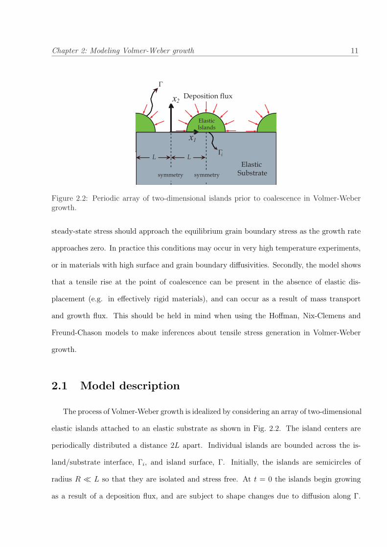


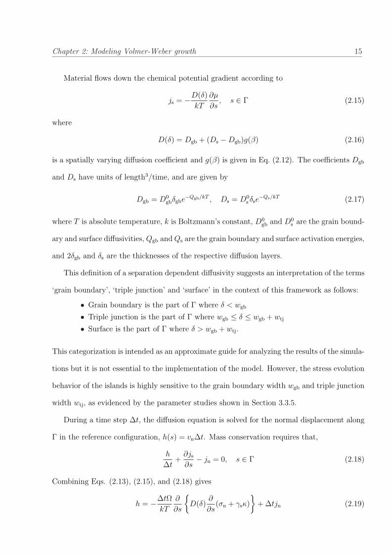


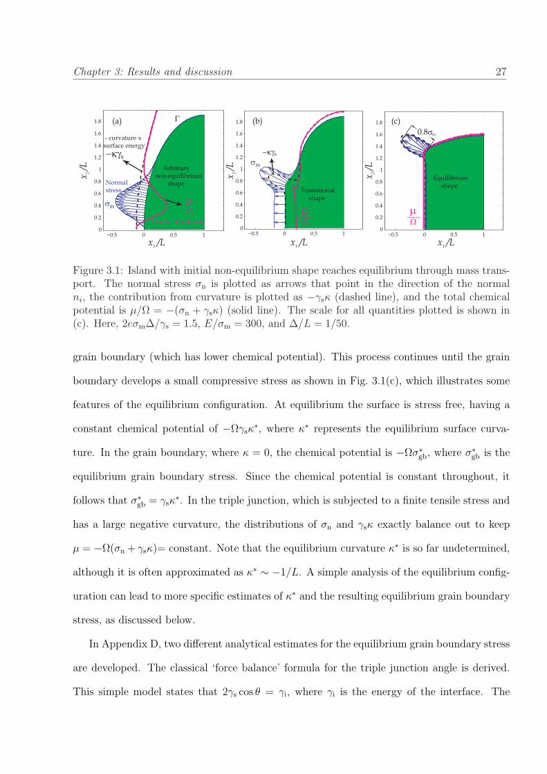
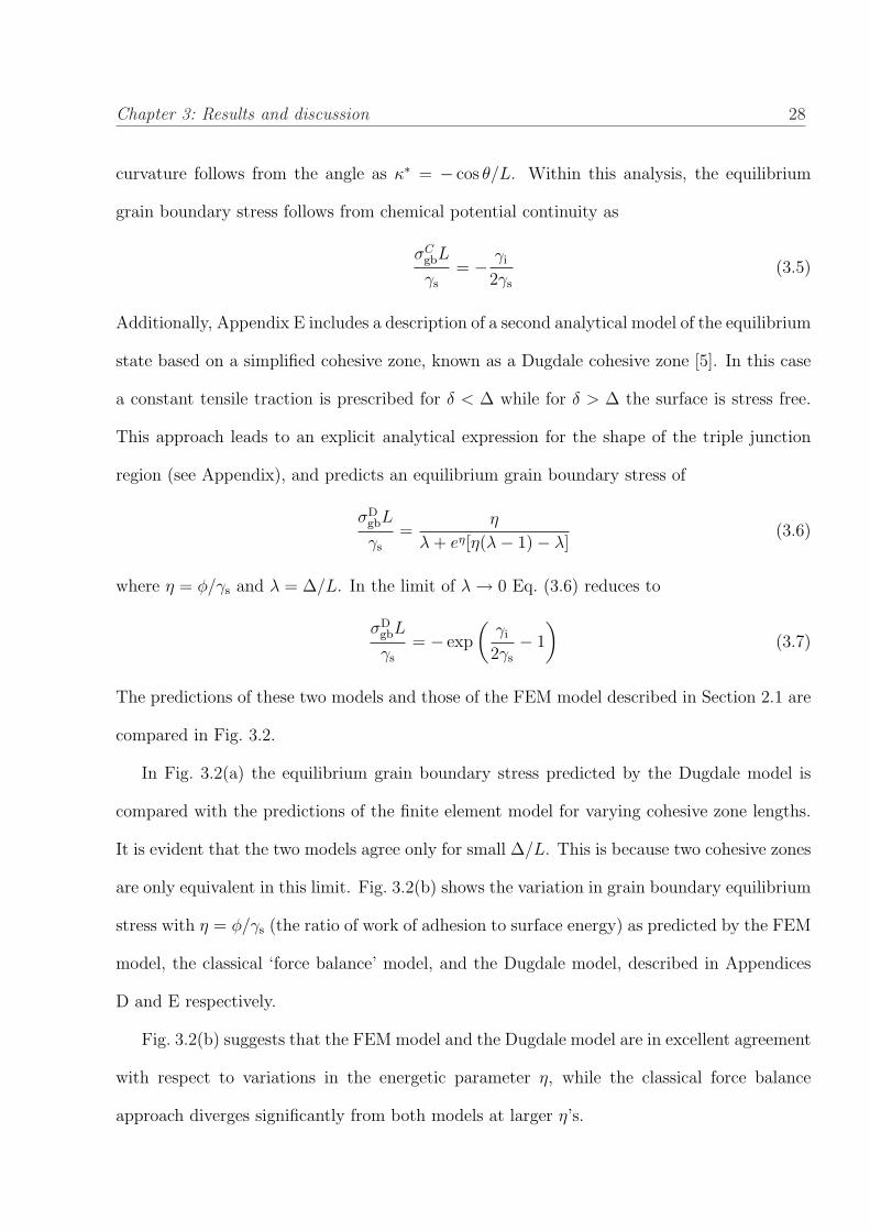
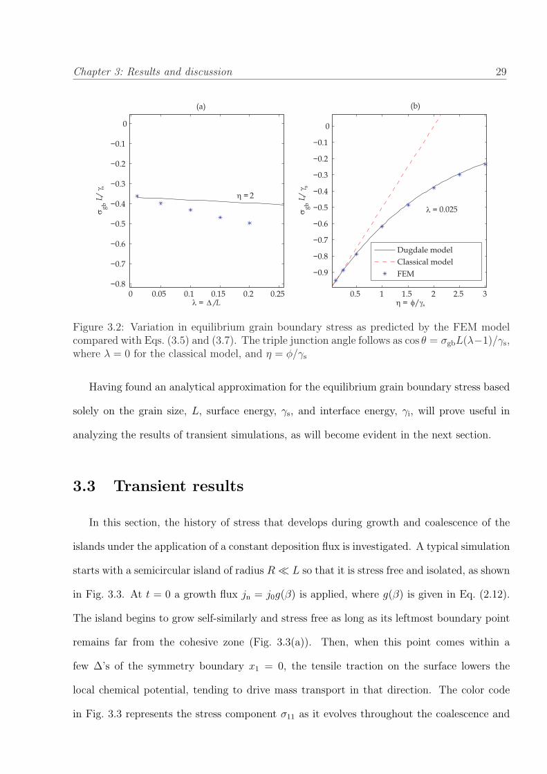
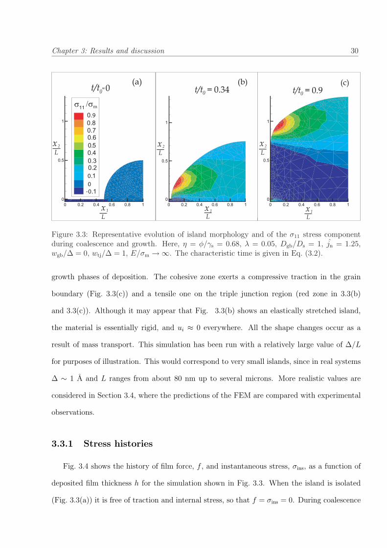
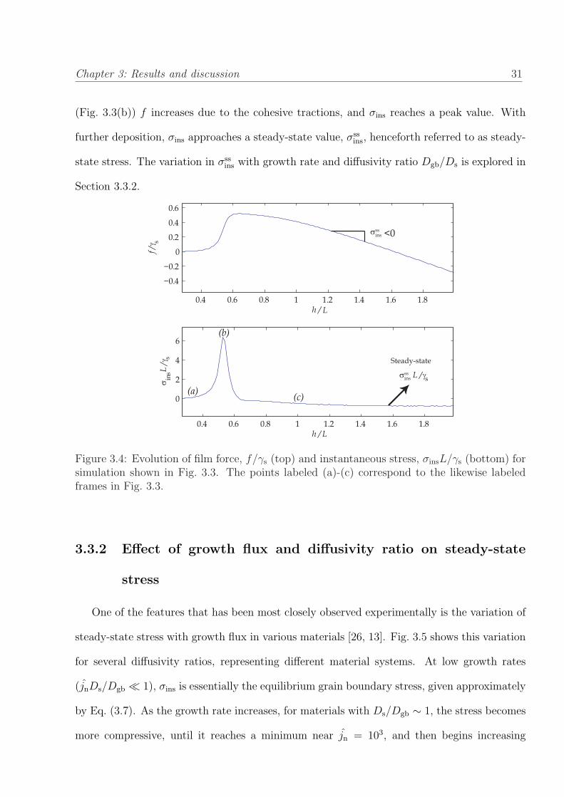

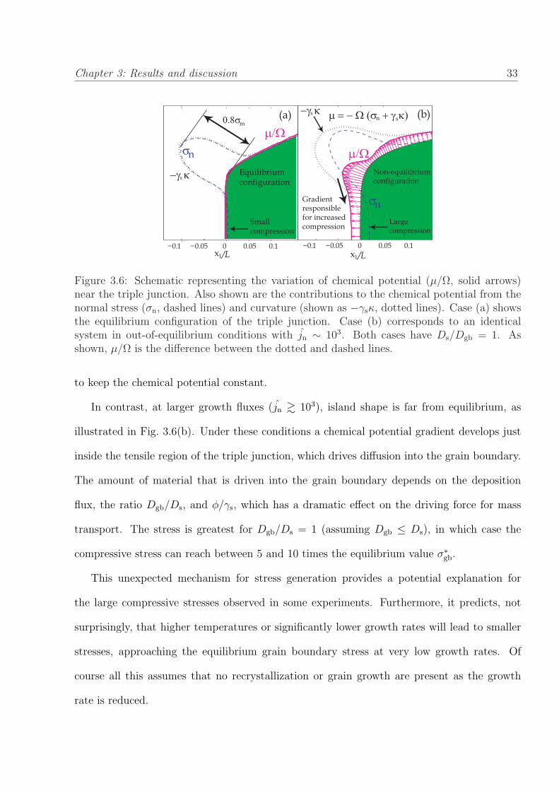


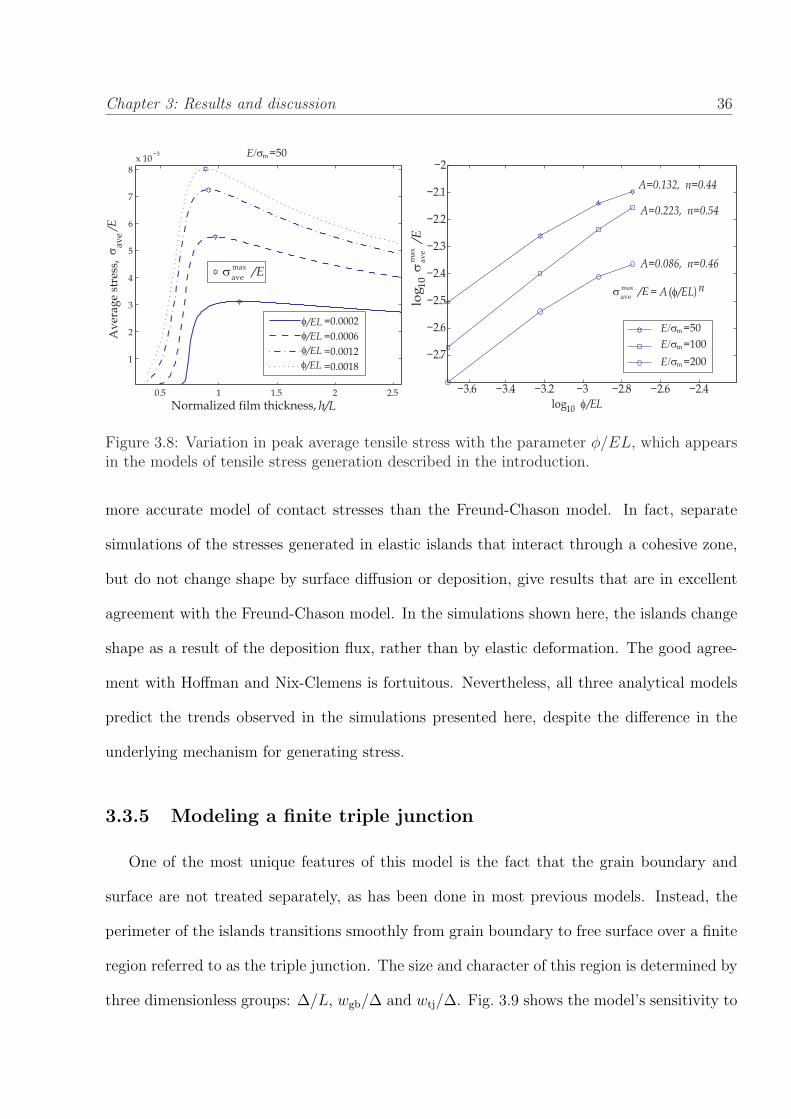
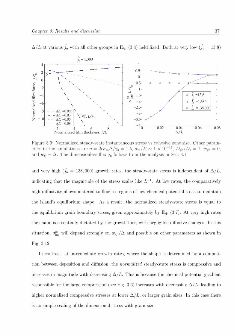
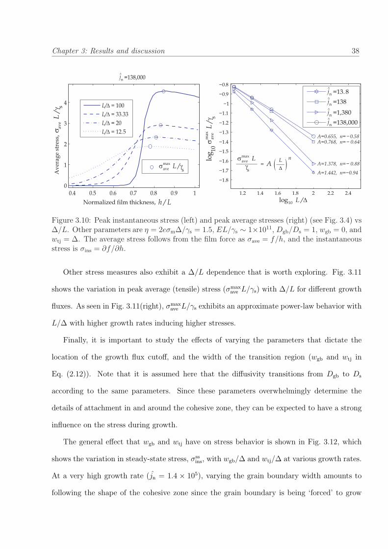


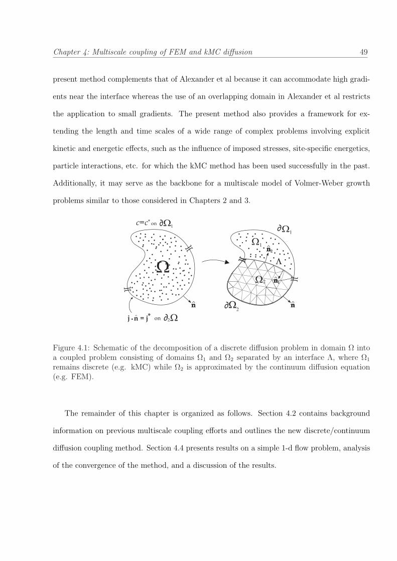

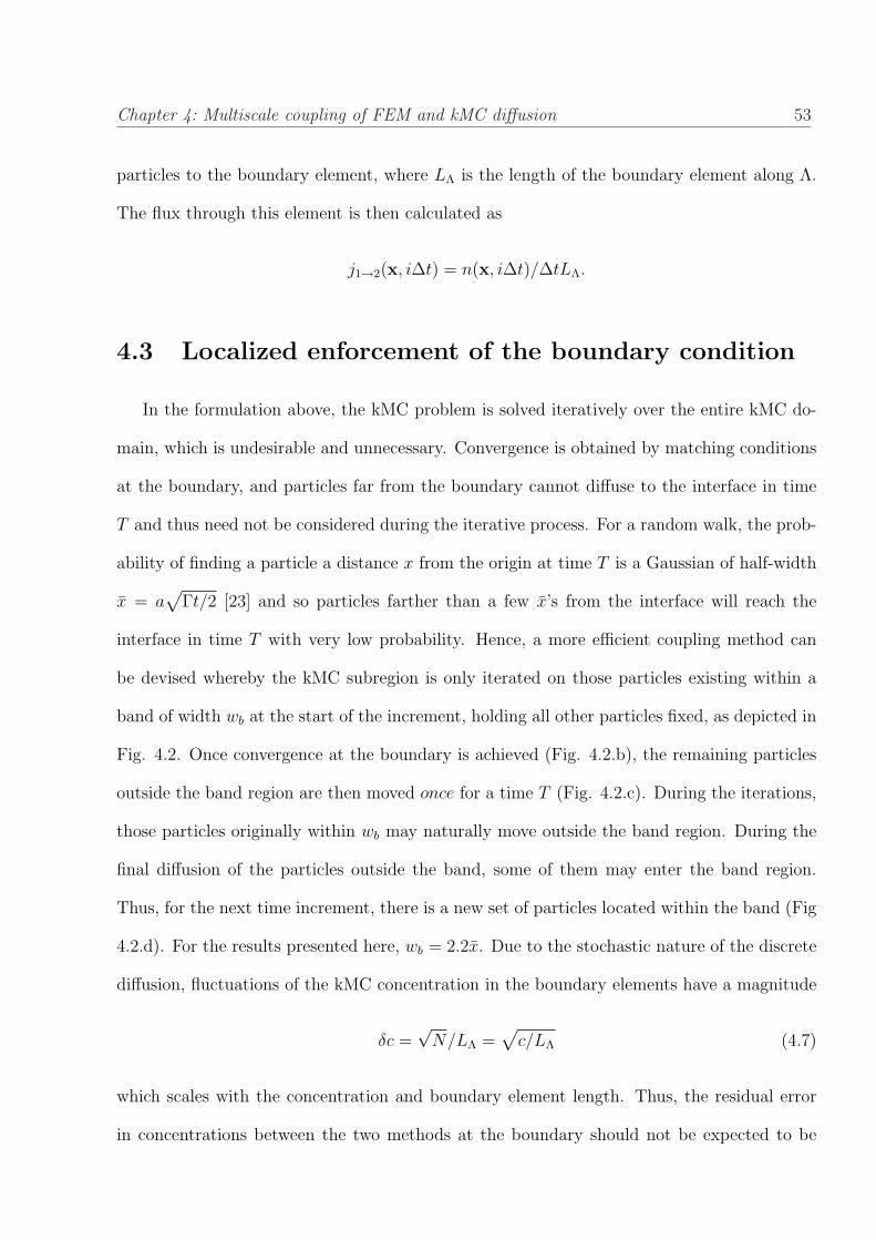


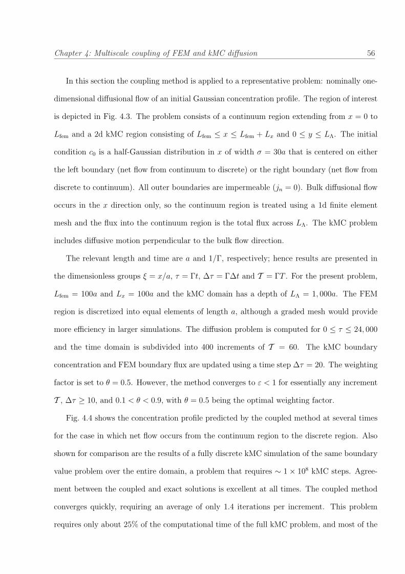
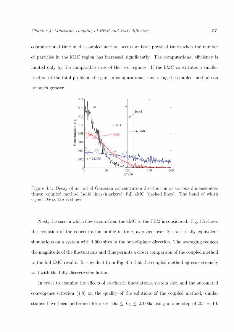
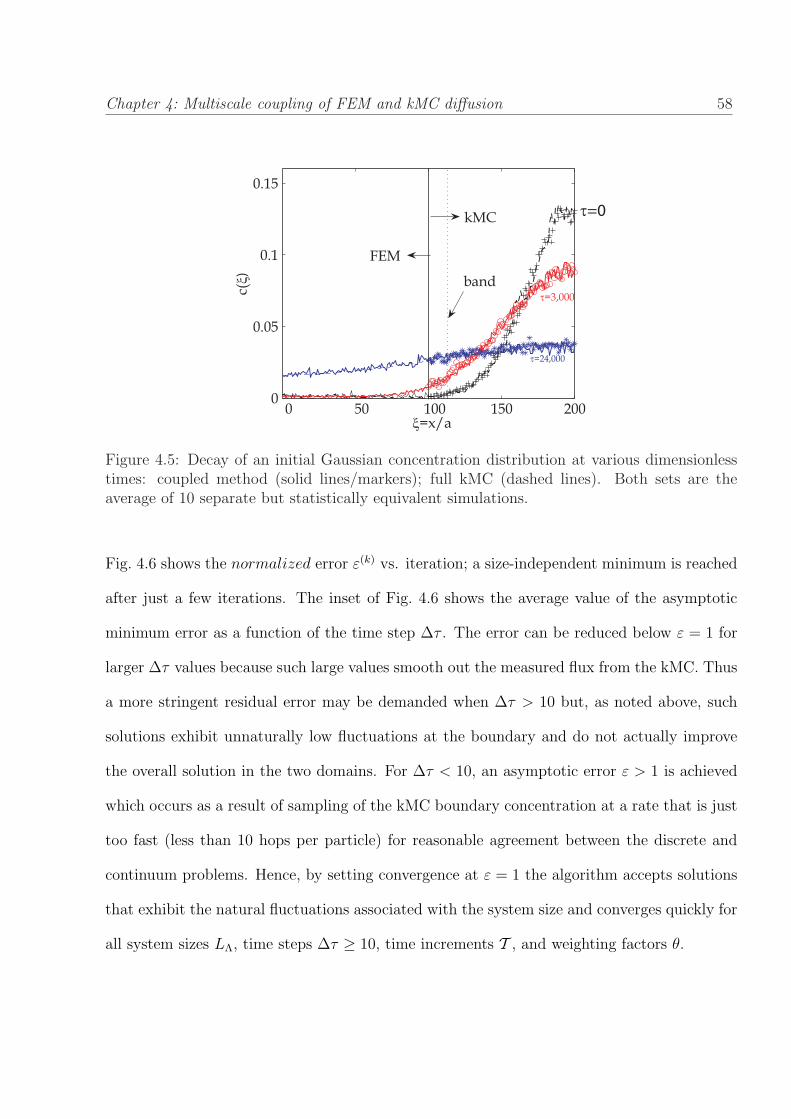

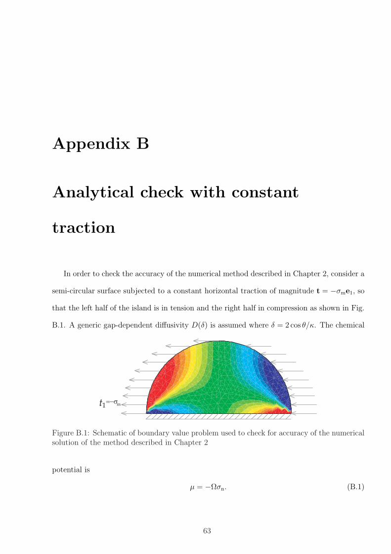
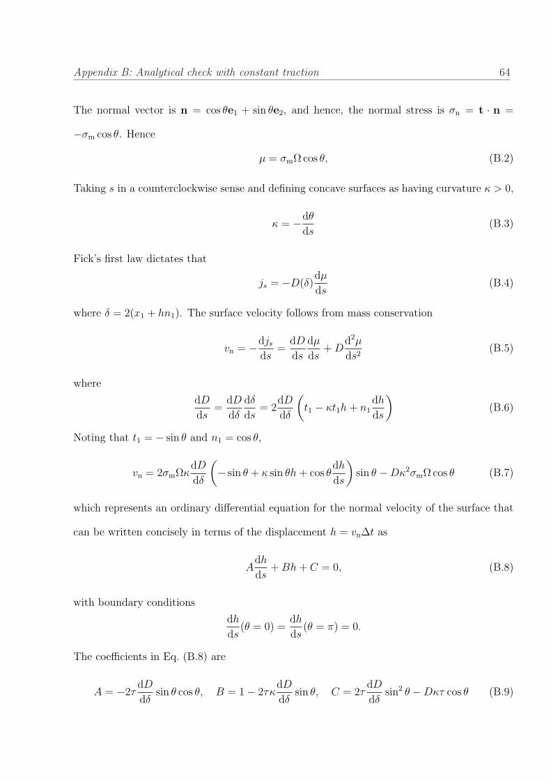

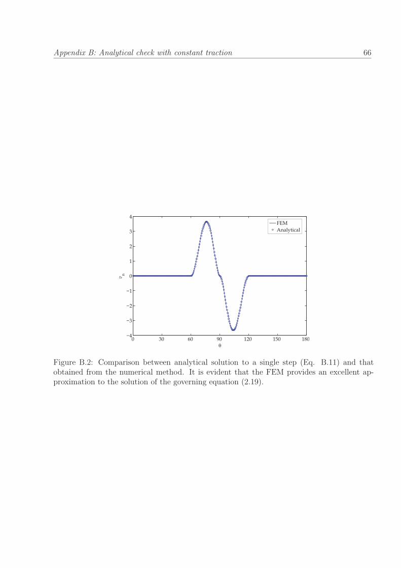
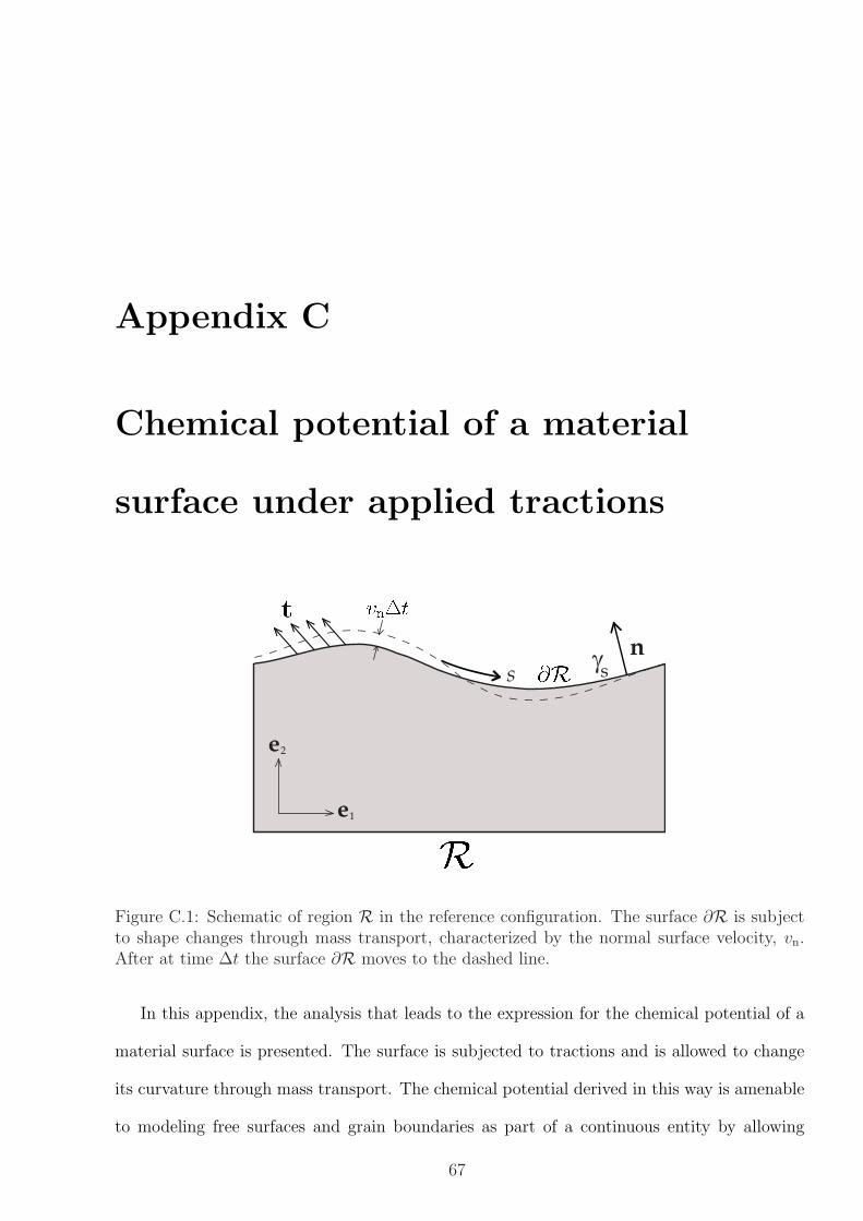
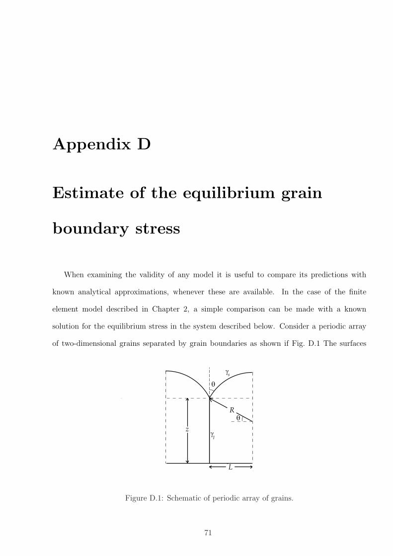


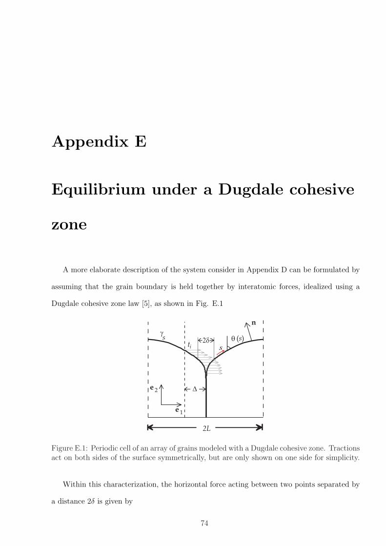


![THESIS TITLE A THESIS SUBMITTED TO THE MIDDLE EAST ...ii.metu.edu.tr/system/files/documents/thesis... · [SAMPLE 1] Approval of the thesis: THESIS TITLE Submitted by STUDENT NAME](https://static.documents.pub/doc/80x56/6019035f39977162fc4f0b03/thesis-title-a-thesis-submitted-to-the-middle-east-iimetuedutrsystemfilesdocumentsthesis.jpg)


