Mark James Brady 182 words

Thesis AbstractIncompleteness and background are two important types of variance found in

images of objects. It has been proposed that a bidirectional network within the visual cortexallows organisms to cope with this variability. In this thesis, the problems of incompletenessand background are defined in detail and various bidirectional (feed- forward and back-projecting) network solutions are proposed and discussed. Three experiments wereperformed to investigate how such a network might recognize objects which are incompleteor backgrounded. In the first experiment, spatial and temporal manipulations of illusorycontours are used to test the hypothesis that a bidirectional network is responsible forillusory contour formation. In the second experiment, incomplete and backgroundedversions of the same object are studied to test the hypothesis that the real purpose of neuralback projections is segmentation rather than object completion. And, in the thirdexperiment, novel camouflage objects are used to study the ability or inability of the brain tolearn new object representations, when the brain is without the benefit of active backprojections.

UNIVERSITY OF MINNESOTA

This is to certify that I have examined this copy of a doctoral thesis by

Mark James Brady

and have found it complete and satisfactory in all respects,and that any revisions required by the final

examining committee have been made.

Daniel J. Kersten_____________________________________________________

______________________________________________________

Signature of Faculty Adviser

______________________________________________________

Date

GRADUATE SCHOOL

PSYCHOPHYSICAL INVESTIGATIONS OF INCOMPLETE FORMS ANDFORMS WITH BACKGROUND

A THESISSUBMITTED TO THE FACULTY OF THE GRADUATE SCHOOL

OF THE UNIVERSITY OF MINNESOTABY

Mark James Brady

IN PARTIAL FULFILLMENT OF THE REQUIREMENTSFOR THE DEGREE OF

DOCTOR OF PHILOSOPHY

Daniel Kersten, Advisor

March 1999

” Mark James Brady 1999

i

AcknowledgementsI would like to thank the committee; Professors Georgopoulos, Kersten, Legge,

Papanikolopoulos, and Tannenbaum, for their valuable time and expertise. I would like to

thank Professor Legge for his leadership of the committee and Professor Kersten for being

my advisor and true mentor.

This work was supported in part by NIH Grant EY02857.

AbstractIncompleteness and background are two important types of variance found in

images of objects. It has been proposed that a bidirectional network within the visual cortexallows organisms to cope with this variability. In this thesis, the problems of incompletenessand background are defined in detail and various bidirectional (feed- forward and back-projecting) network solutions are proposed and discussed. Three experiments wereperformed to investigate how such a network might recognize objects which are incompleteor backgrounded. In the first experiment, spatial and temporal manipulations of illusorycontours are used to test the hypothesis that a bidirectional network is responsible forillusory contour formation. In the second experiment, incomplete and backgroundedversions of the same object are studied to test the hypothesis that the real purpose of neuralback projections is segmentation rather than object completion. And, in the thirdexperiment, novel camouflage objects are used to study the ability or inability of the brain tolearn new object representations, when the brain is without the benefit of active backprojections.

PrefaceThis thesis is about the perception of incomplete and backgrounded objects. Both

incompleteness and background are under appreciated aspects of the vision problem. While

incompleteness has been studied to some extent, in the form of illusory contour figures for

example, the extent to which incompleteness actually occurs in natural images is probably

underestimated by most. Background in natural images has been studied relatively little,

ii

perhaps due to difficulties in experimental design. Both incompleteness and background are

sources of variance in image formation and variance is the crux problem to solve before we

understand how vision is accomplished. One assumption which is made and analyzed

throughout the thesis is that high level models are used to overcome the ambiguities which

arise due to background and incompleteness related variance. A bidirectional network is

required to carry incoming visual data from early stages of processing to higher stages and to

carry high level model data back to earlier levels of visual cortex.

The thesis begins by stating some first principles which define the task of vision. This

may seem overly obvious to some readers. However, if this is not done, I would risk the

greater flaw of jumping into a discourse with the reader not knowing where I am going or

why. Hopefully, this first principles approach will get all readers off on the same foot. Also,

after reading the theoretical section, the reader will see that not every investigator picks the

same first principles. Therefore, these first principles may not be so obvious after all.

After establishing a definition of vision, I next describe the problems which a visual

system must overcome to fulfill its purpose, with an emphasis on variance. The magnitude of

the difficulty of solving the vision problem can be fully appreciated if one has some

familiarity with many of the subtasks which biological systems successfully carry out, and if

one has made some attempts to reproduce some of these capabilities in a computer (machine

vision). Therefore, I describe the relation between research of biological vision and research

of machine vision.

Next is a rather complete, yet concise, section on the functional neuroanatomy of the

visual cortex. Many theories of vision are based on the anatomical, as well as the functional

properties of biological vision systems. Since, I found no one place where this functional

anatomical information is collected together, I include it in the background chapter. As well

as serving as a reference for the sections on theory, the reader should find it to be a useful

reference in general. One alternative to making the anatomy section complete would be to

only refer to specific details which will be directly relevant to the experiments and theory.

iii

However, because the parts of the visual cortex are so highly integrated, it is difficult to

capture any sense of its organization in a piecemeal fashion.

The section on theory provides the raw material for the hypotheses which are tested in

the experiments. In the section on theory, a number of references are cited. I try to include

enough information with each reference so that the reader is not left with the task of library

research, simply in order to understand the current work. This style, taken to extremes, would

result in a review. However, this is avoided since my expansions on these citations include

interpretations of results which are not necessarily the same as the original authors. There are

also changes of notation, derivations and reinterpretations of mathematics; either to clarify the

mathematics or to make it relevant to the vision context. Then, I make connections among

the cited works and to the experiments of this thesis.

Finally, comes the experiments. These are designed to shed light on questions of

incomplete and backgrounded object perception, which have been raised previously in the

background section. The three experiments performed for this thesis are all

psychophysical.

Chapter 2 covers experiment 1, which investigates the temporal characteristics of

illusory contours; illusory contours being generated by incomplete figures. In experiment 1,

the interaction of illusory contour generators and near threshold edge elements are

manipulated by temporal delays between the two. The sensitivity at these various delays, are

used to investigate the function of forward and back projecting connections in visual cortex.

Chapter 3 covers experiment 2, which investigates the differences between the

perceptual processes of recognizing incomplete vs. backgrounded objects. In experiment 2,

backgrounded and incomplete stimuli are presented separately and the time required to

recognize these objects is recorded. The histograms of these delay times tell something about

the differences in how backgrounded and incomplete objects are processed.

iv

Chapter 4 covers experiment 3, which investigates the means by which high level

object models are formed. This investigation requires novel objects which blend into or are

camouflaged within their background. This novelty and camouflage makes such objects

unsegmentable from the background. Experiment 3 determines what segmentation clues are

required before observers can learn to recognize objects.

v

Table of Contents1. BACKGROUND 13

1.1 The Task of Seeing 1 3

1.2 Natural Images are Highly Ambiguous 1 4

1.3 Investigating the Visual Mechanism 2 3

1.4 General Principles of Organization in the Visual Cortex 2 3

1.5 Organization and Response Properties of Neurons in the Visual Cortex 2 91.5.1 The Retina... Briefly 291.5.2 The LGN 291.5.3 V1 301.5.4 V2 371.5.5 V3 391.5.6 V4 391.5.7 MT 421.5.8 IT 43

1.6 Theories of Visual Cortex, and Related Theories 5 01.6.1 Bayesian Inference 511.6.2 Bayesian Analysis in Psychophysics 601.6.3 Bayesian Models of Perception 671.6.4 Stochastic Complexity and Minimum Description Length 781.6.5 Redundancy Reduction 841.6.6 Binding and Exclusion 881.6.7 Bidirectional Models 911.6.8 Theoretical Background of the Experiments 112

2. EXPERIMENT 1: SPATIAL AND TEMPORAL ASYMMETRIES OFILLUSORY CONTOUR FORMATION 121

2.1 Introduction 1 2 1

2.2 Methods 1 2 92.2.1 Apparatus & Software 1292.2.2 Observers 1322.2.3 Stimuli 1322.2.4 Experimental Design 135

2.3 Results 1 4 22.3.1 Non-SOA Controls 1422.3.2 Bull’s Eye Controls 1452.3.3 Modal - Bull 1482.3.4 Amodal - Bull 1512.3.5 Modal Zero Degrees 153

vi

2.4 Discussion 1 5 6

3. EXPERIMENT 2: TEMPORAL PATTERNS IN THE PERCEPTION OFBACKGROUNDED AND INCOMPLETE OBJECTS 158

3.1 Introduction 1 5 8

3.2 Methods 1 6 53.2.1 Stimuli 1653.2.2 Observers 1773.2.3 Procedure 177

3.3 Results 1 7 8

3.4 Discussion 1 8 5

4. EXPERIMENT 3: LEARNING TO RECOGNIZE NOVELCAMOUFLAGED OBJECTS 186

4.1 Introduction 1 8 6

4.2 Purpose of the Experiment and Summary of Methods 1 8 7

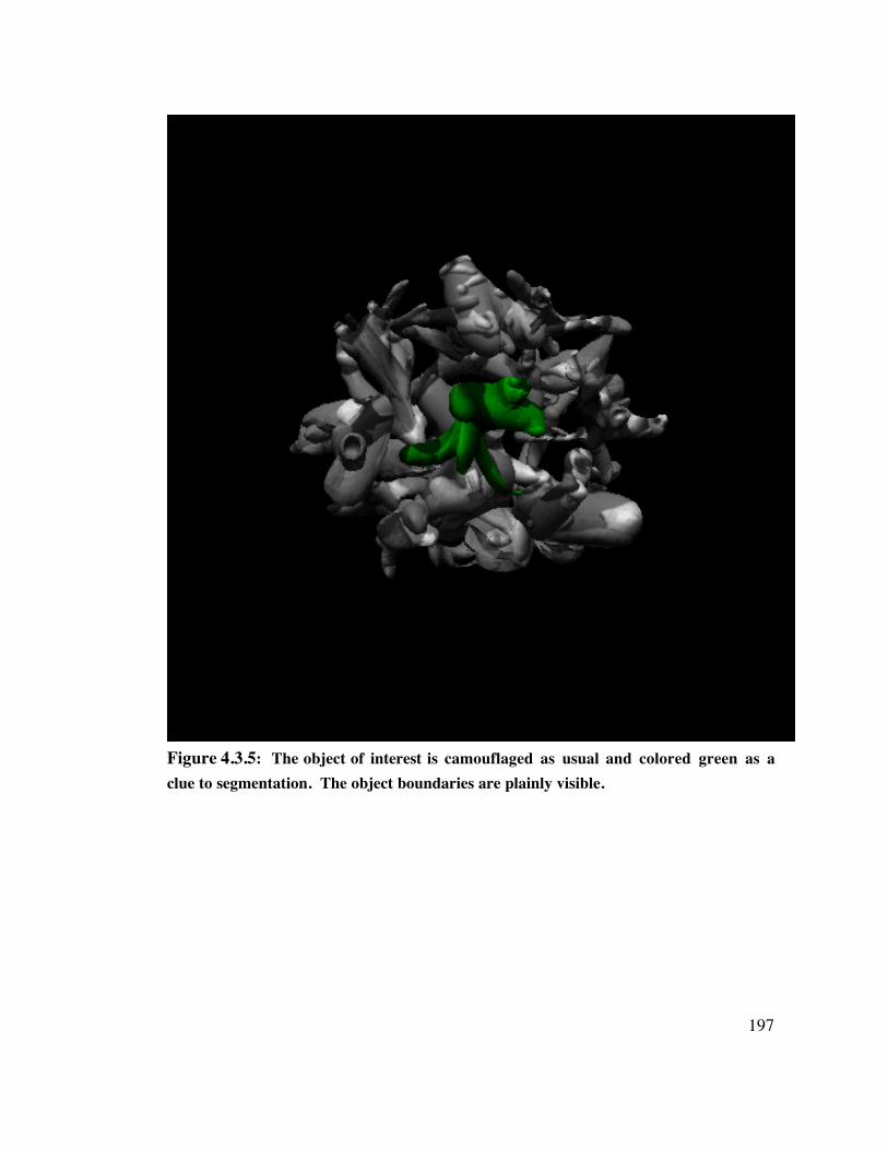
4.3 Methods 1 8 84.3.1 Creation of Novel Objects 1884.3.2 Scene Construction 1914.3.3 Observers 1914.3.4 Testing - Training Design 1914.3.5 Training 1924.3.6 Testing 193

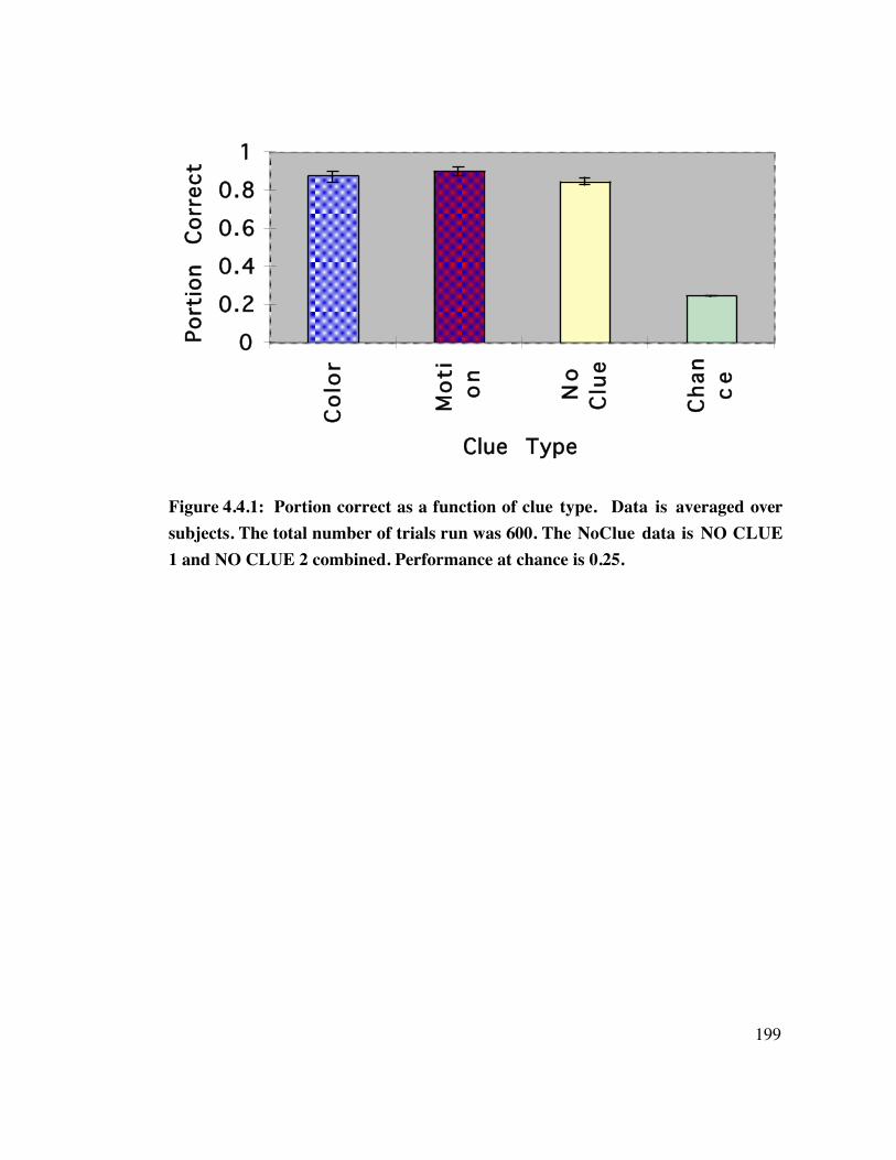
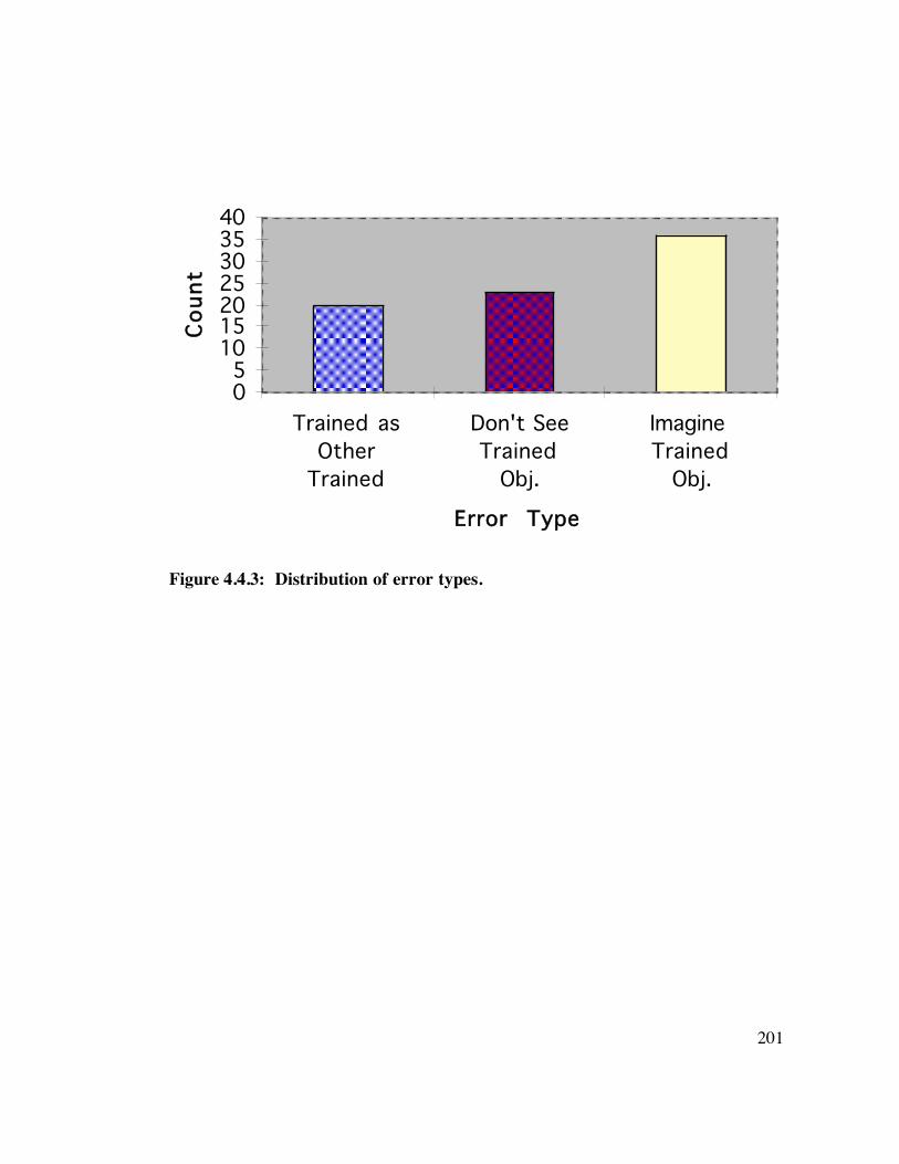
4.4 Results 1 9 8

4.5 Discussion 2 0 5

5. SUMMARY 209

6. APPENDIX A: ALGORITHM FOR GENERATING DIGITAL EMBRYOS211

6.1 2 1 1

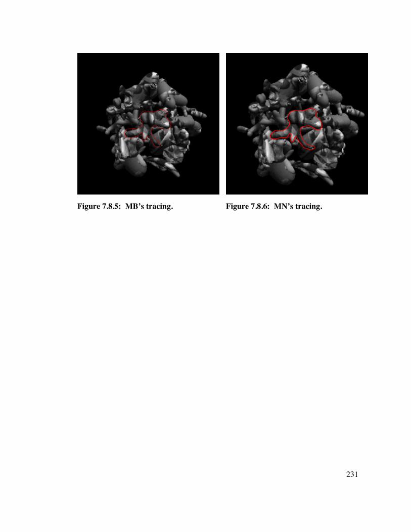
7. APPENDIX B: EXPERIMENT 3 TRACING RESULTS 215

7.1 NO CLUE 1, Object A 2 1 5

7.2 NO CLUE 1, Object B 2 1 8

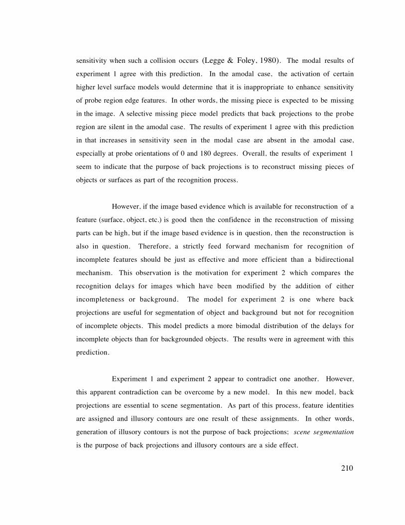
7.3 NO CLUE 1, Object C 2 2 0

vii

7.4 MOTION, Object A 2 2 2

7.5 MOTION, Object B 2 2 4

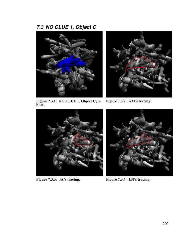
7.6 MOTION, Object C 2 2 6

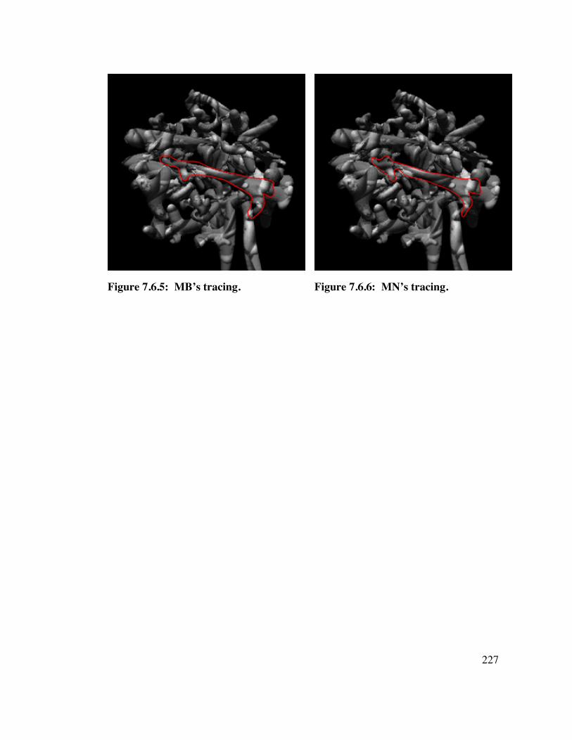
7.7 COLOR, ObjectA 2 2 8

7.8 COLOR, Object B 2 3 0

7.9 COLOR, Object C 2 3 2

7.10 NO CLUE 2, Object A 2 3 4

7.11 NO CLUE 2, Object B 2 3 6

7.12 NO CLUE 2, Object C 2 3 8

viii

Table of FiguresFigure 1.2.1: A scene from the peak of Mount Elbert, Colorado....................................................... 17

Figure 1.2.2: An eyelash viper waits in the branches of a mango tree.. .............................................. 18

Figure 1.2.3: The stripes of these zebras provide destructive camouflage .......................................... 20

Figure 1.2.4: A caterpillar uses skin pigment to mimic a snake ...................................................... 22

Figure 1.5.1: A schematic of connections within V1 layers. ........................................................... 32

Figure 1.5.2: Gabor shaped receptive fields of V1 neurons.............................................................. 33

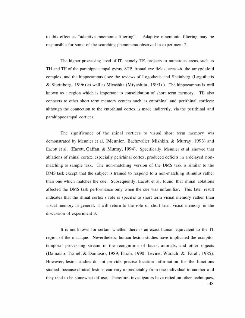
Figure 1.6.1: External and internal visual spaces. ......................................................................... 53

Figure 1.6.2: Any number of 3D wireframes can project onto the same image. .................................. 56

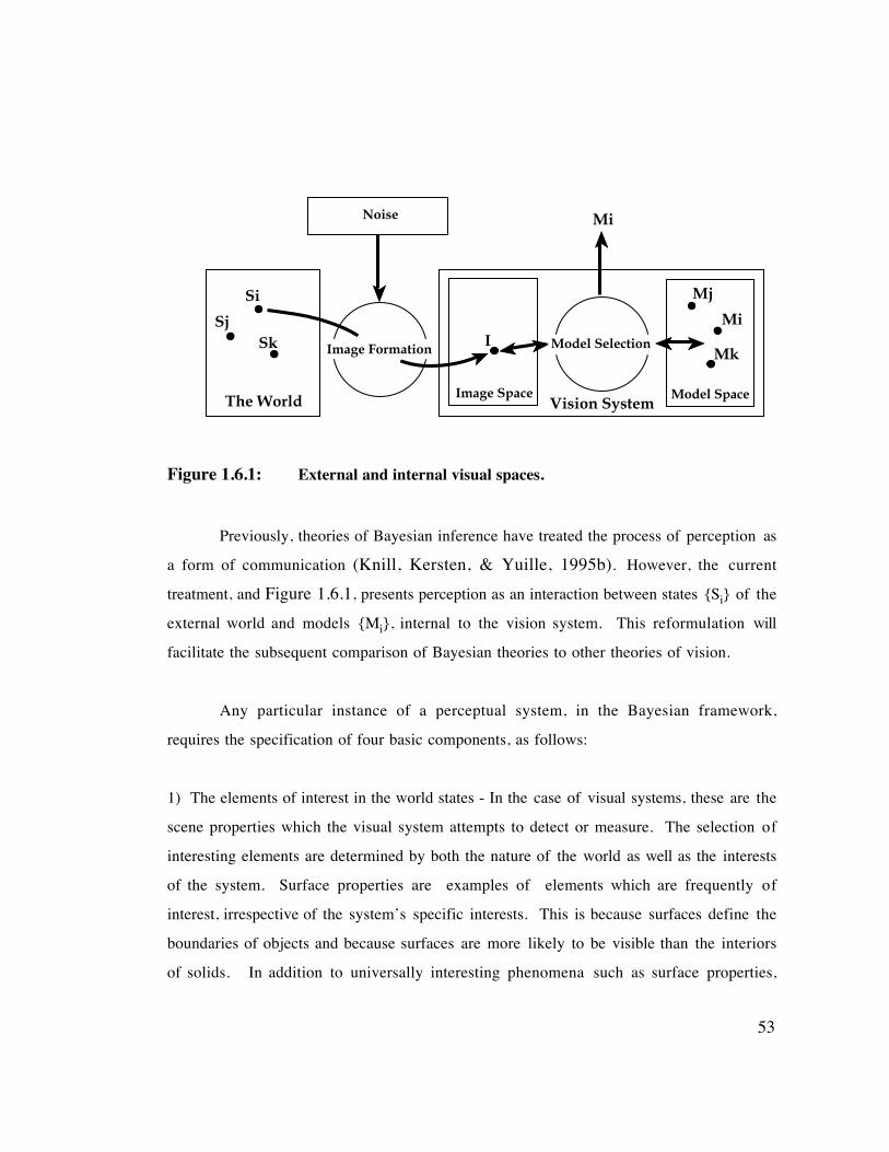
Figure 1.6.3: Other than the shadows, both images are the same......................................................62

Figure 1.6.4: (b) and (c) are identical except for the shadows............................................................62

Figure 1.6.5: An example likelihood distribution for some fixed image I and model Hi........................ 71

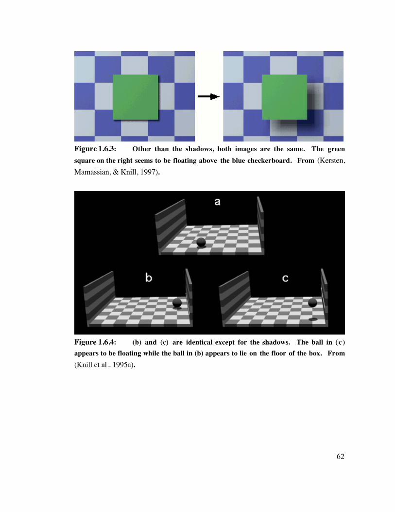
Figure 1.6.6: An example prior probability distribution................................................................. 72

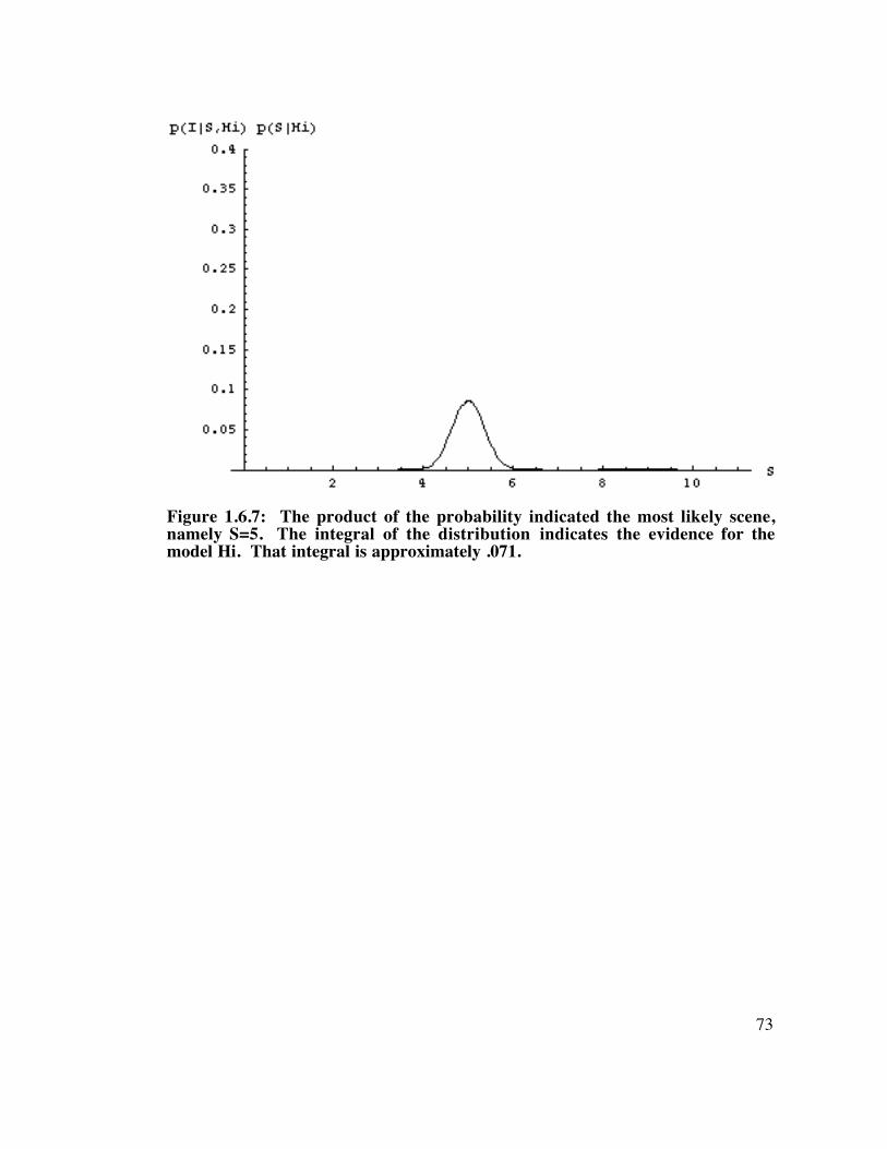
Figure 1.6.7: The product of the probability indicated the most likely scene. ..................................... 73

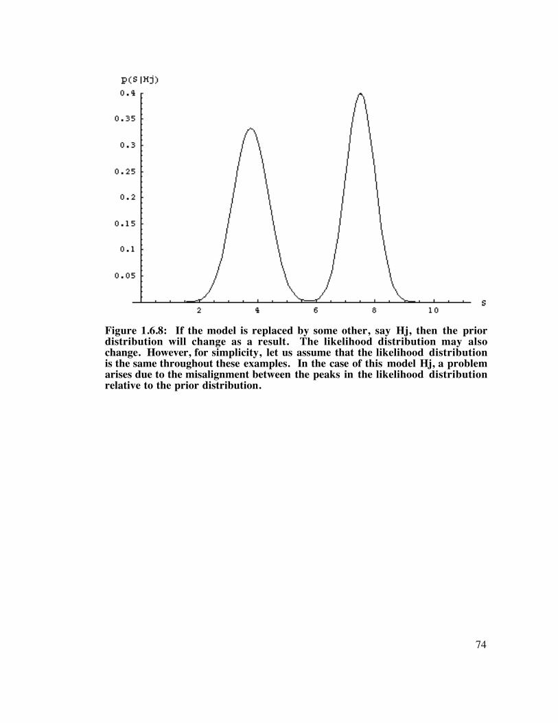
Figure 1.6.8: A problem arises due to the misalignment between the peaks. ...................................... 74

Figure 1.6.9: The product of the likelihood and the prior under the model Hj. .................................... 75

Figure 1.6.10: Yet another model, Hk, suffers from being too general.. ............................................ 76

Figure 1.6.11: Once again, the best choice of scene is not so clear................................................... 77

Figure 1.6.12: An apparently simple image of a book on a shelf..................................................... 93

Figure 1.6.13: Oriented contrast image. ...................................................................................... 94

Figure 1.6.14: Circuit for detecting direction of motion in the ROI model......................................... 97

Figure 1.6.15: Partially tuned directional neurons are fully tuned..................................................... 98

Figure 1.6.16: This circuit takes aligned end stopped responses as evidence ......................................100

Figure 1.6.17: An illusory contour appears between two gratings...................................................101

Figure 1.6.18: Real edges which cross illusory contour ................................................................103

Figure 1.6.19: The illusory contours in the figure on the left are easily seen.....................................105

Figure 1.6.20: The Ehrenstein illusion......................................................................................106

Figure 1.6.21: Center surround cells of the LGN..........................................................................107

Figure 1.6.22: A small portion of the BCS / FCS model...............................................................108

Figure 1.6.23: Feature Hierarchy Principle. ................................................................................115

Figure 1.6.24: A subnet inspired by the Missing Piece Principle. ..................................................118

Figure 1.6.25: This subnet is similar to the LGN<->V1 subnet .....................................................119

ix

Figure 1.6.26: Subnet inspired by the Unique Ownership Principle..................................................120

Figure 2.1.1: The perception of an occluding square......................................................................123

Figure 2.1.2: Kanisza square with labeled features........................................................................126

Figure 2.1.3: Missing Piece Net capable of generating illusory contours...........................................127

Figure 2.2.1: Stereoscope design, top view. ...............................................................................130

Figure 2.2.2: Stereoscope design, side view. ..............................................................................131

Figure 2.2.3: The bull’s eye stimulus. ......................................................................................134

Figure 2.2.4: 2D rendition of amodal Kanizsa square stimulus. .......................................................137

Figure 2.2.5: Modal factor combinations ...................................................................................138

Figure 2.2.6: Amodal factor combinations. ................................................................................139

Figure 2.2.7: Bull factor combinations. .....................................................................................140

Figure 2.3.1: Main effect of non-SOA control conditions..............................................................143

Figure 2.3.2: Main effect of observer sensitivity .........................................................................144

Figure 2.3.3: Contrast threshold as a function of edgel orientation..................................................146

Figure 2.3.4: Contrast threshold as a function of SOA .................................................................147

Figure 2.3.5: Contrast threshold as a function of orientation..........................................................149

Figure 2.3.6: Contrast threshold as a function of SOA .................................................................150

Figure 2.3.7: Contrast threshold as a function of orientation..........................................................152

Figure 2.3.8: Interaction effect between orientation and SOA.........................................................153

Figure 2.3.9: Contrast threshold as a function of SOA. ................................................................154

Figure 2.3.10: Interaction of observer*SOA. ..............................................................................155

Figure 3.1.1: This image of a dog relies on the natural mechanisms of homeochromatic camouflage.....159

Figure 3.1.2: A completion net.................................................................................................161

Figure 3.1.3: A segmentation net.............................................................................................164

Figure 3.2.1: Complete version of an actual badger skull. .............................................................167

Figure 3.2.2: Complete version of a boat. .................................................................................168

Figure 3.2.3: Complete version of a stingray.. ...........................................................................169

Figure 3.2.4: Backgrounded version of a badger skull. ..................................................................170

Figure 3.2.5: Backgrounded version of a boat..............................................................................171

Figure 3.2.6: Backgrounded version of a stingray. The background is a brass plate............................172

Figure 3.2.7: Incomplete version of a badger skull.......................................................................173

Figure 3.2.8: Incomplete version of a boat. ................................................................................174

Figure 3.2.9: Incomplete version of a stingray. ...........................................................................175

Figure 3.2.10: Mask image.....................................................................................................176

Figure 3.3.1: Control case of complete objects having no background.............................................180

x

Figure 3.3.2: Background case .................................................................................................181

Figure 3.3.3: Incomplete case. ................................................................................................182

Figure 4.3.1: Two fully grown digital embryos...........................................................................190

Figure 4.3.2: Camouflaged novel objects with a background..........................................................194

Figure 4.3.3: Another scene Example.........................................................................................195

Figure 4.3.4: Another scene example ........................................................................................196

Figure 4.3.5: The object of interest is camouflaged as usual and colored green ...................................197

Figure 4.4.1: Portion correct as a function of clue type.................................................................199

Figure 4.4.2: Portion correct as a function of subject ....................................................................200

Figure 4.4.3: Distribution of error types. ....................................................................................201

Figure 4.4.4: MN’s tracing of NO CLUE 1, object C. ...............................................................203

Figure 4.4.5: MB’s tracing of NO CLUE ................................................................................203

Figure 4.4.6: AM’s tracing of NO CLUE 1..............................................................................204

Figure 4.5.1: Model explaining the phenomenon of bootstrapped learning........................................206

Figure 6.1.1: Triangle DEF before and after fission.......................................................................213

Figure 7.1.1: NO CLUE 1, object A, no camo, shown in blue for reference. .....................................216

Figure 7.1.2: Observer AM’s tracing. Note incorrect position........................................................216

Figure 7.1.3: JA’s tracing. Some parts are omitted while others are incorrectly added..........................216

Figure 7.1.4: LN claimed an inability to trace. ............................................................................216

Figure 7.1.5: MB’s tracing is correct except for some missing parts.................................................217

Figure 7.1.6: MN’s tracing. She recognized a portion of the object..................................................217

Figure 7.2.1: Reference image for.............................................................................................218

Figure 7.2.2: AM’s tracing. ....................................................................................................218

Figure 7.2.3: JA’s tracing. ......................................................................................................218

Figure 7.2.4: LN’s tracing. An imaginary portion is included on the left.........................................218

Figure 7.2.5: MB’s tracing. .....................................................................................................219

Figure 7.2.6: MN’s tracing. ....................................................................................................219

Figure 7.3.1: NO CLUE 1, Object C, in blue.............................................................................220

Figure 7.3.2: AM’s tracing. ....................................................................................................220

Figure 7.3.3: JA’s tracing. ......................................................................................................220

Figure 7.3.4: LN’s tracing. .....................................................................................................220

Figure 7.3.5: Tracing data of MB for this object was either not recorded or it was lost. .......................221

Figure 7.3.6: MN’s tracing. ....................................................................................................221

Figure 7.4.1: MOTION, Object A reference. Segmented and shown with camouflage. .........................222

Figure 7.4.2: AM’s tracing. ....................................................................................................222

xi

Figure 7.4.3: Like AM’s placement error...................................................................................223

Figure 7.4.4: LN’s tracing. .....................................................................................................223

Figure 7.4.5: MB’s tracing......................................................................................................223

Figure 7.4.6: MN’s tracing. ....................................................................................................223

Figure 7.5.1: Reference view of MOTION, Object B....................................................................224

Figure 7.5.2: AM’s tracing, one of the best................................................................................224

Figure 7.5.3: JA’s tracing. ......................................................................................................224

Figure 7.5.4: LN’s tracing. .....................................................................................................224

Figure 7.5.5: MB’s tracing......................................................................................................225

Figure 7.5.6: MN’s tracing. ....................................................................................................225

Figure 7.6.1: Reference view of MOTION, Object C. ..................................................................226

Figure 7.6.2: AM’s tracing. ....................................................................................................226

Figure 7.6.3: JA’s tracing. ......................................................................................................226

Figure 7.6.4: LN’s tracing. .....................................................................................................226

Figure 7.6.5: MB’s tracing......................................................................................................227

Figure 7.6.6: MN’s tracing. ....................................................................................................227

Figure 7.7.1: Reference image of COLOR, Object A, shown in color and camouflage. .......................228

Figure 7.7.2: AM’s tracing. ....................................................................................................228

Figure 7.7.3: For JA, this simple object proved difficult, even after color clue training.......................228

Figure 7.7.4: LN’s tracing. .....................................................................................................228

Figure 7.7.5: MB also had trouble tracing this simple object .........................................................229

Figure 7.7.6: MN’s tracing. ....................................................................................................229

Figure 7.8.1: Reference view of COLOR, Object B. .....................................................................230

Figure 7.8.2: AM’s tracing. ....................................................................................................230

Figure 7.8.3: JA’s tracing. ......................................................................................................230

Figure 7.8.4: LN’s tracing. .....................................................................................................230

Figure 7.8.5: MB’s tracing......................................................................................................231

Figure 7.8.6: MN’s tracing. ....................................................................................................231

Figure 7.9.1: Reference view of COLOR, Object C. ....................................................................232

Figure 7.9.2: AM’s tracing. ....................................................................................................232

Figure 7.9.3: JA’s tracing. ......................................................................................................232

Figure 7.9.4: LN’s tracing. .....................................................................................................232

Figure 7.9.5: MB’s tracing......................................................................................................233

Figure 7.9.6: MN’s tracing. .....................................................................................................233

Figure 7.10.1: Reference view of NO CLUE 2, Object A, shown in blue with no camouflage. ............234

xii

Figure 7.10.2: AM’s tracing....................................................................................................234

Figure 7.10.3: JA’s tracing. ....................................................................................................234

Figure 7.10.4: LN’s tracing.....................................................................................................234

Figure 7.10.5: MB’s tracing. ...................................................................................................235

Figure 7.10.6: MN’s tracing....................................................................................................235

Figure 7.11.1: Reference view of NO CLUE 2, Object B. .............................................................236

Figure 7.11.2: AM’s tracing, possibly overwritten by JA’s. ..........................................................236

Figure 7.11.3: JA’s tracing. ....................................................................................................236

Figure 7.11.4: LN’s tracing.....................................................................................................236

Figure 7.11.5: MB’s tracing. ...................................................................................................237

Figure 7.11.6: MN’s tracing....................................................................................................237

Figure 7.12.1: Reference view of NO CLUE 2, Object C..............................................................238

Figure 7.12.2: AM’s tracing....................................................................................................238

Figure 7.12.3: JA’s tracing. ....................................................................................................238

Figure 7.12.4: LN’s tracing.....................................................................................................238

Figure 7.12.5: MB’s tracing. ...................................................................................................239

Figure 7.12.6: MN’s tracing....................................................................................................239

___________

13

_______________1. Background1.1 The Task of Seeing

In a forest scene, from Shakespeare’s As You Like It, the character Jaques begins

his monologue on life by saying: “All the world’s a stage, And all the men and women

merely players.” As animals, evolution has cast us into a role where our goals are to

survive, reproduce, and perhaps to do something more. Whatever the details of our

casting, we must navigate across the stage of our environment. And, before we can read

our lines to the other players, props, or objects; we must first locate and recognize those

which might have some significance to us.

Like the stage itself, not everything in the world is a proper object. Objects are

generally regarded as things having compact extent and distinct surfaces. Given such a

description for the class of objects: Is a road an object? What about a beach, the surface of

an ocean, or fog? Such things are better thought of as surfaces and materials, rather than

objects. Thus there are three high level components in our scenes: objects, surfaces and

materials.

Objects may be grouped into two subclasses, those with specific and those with

statistically defined shapes. The shapes of rocks and clouds are somewhat random, and the

very fact that we recognize them, is a mystery which lies outside most theories of vision.

Perhaps it is better to think of randomly shaped object classes as materials rather than

proper objects. On the other hand, there are shape characteristics which distinguish rocks

from clouds, there are shape characteristics which distinguish igneous rocks from

metamorphic rocks, and there are shape characteristics which distinguish cirrus clouds

from cumulus clouds. These shape characteristics exist in spite of the fact that there does

not exist any specific shape which defines a rock or a cloud. Given these shape

characteristics, one might agree to classify randomly shaped lumps of material as objects

14

after all. Apparently, there is no distinct boundary between the world of objects and the

world of materials.

Surfaces and materials play multiple roles with respect to a seeing animal. As

already discussed, a surface may be relevant as something to navigate across. Even the act

of grasping can be included as a kind of manual navigation. Whether navigation is pedal

or manual, it is the act of moving one’s self with respect to a surface. On the other hand, a

surface may be simply be part of an object, and understanding which surface shapes

appear in what spatial relation to other surfaces, helps an organism identify the object.

The dual role of a material is as a kind of degenerate object and as an object component.

Given any object independent material, the animal wants to know what it is, so that

appropriate behaviors can be selected. The animal wants to know if it should dig in this

material, swim through it, or consume it. However, if the material is thought of as a part of

an object, then identifying the material helps to identify the object. In summary then, the

task of vision amounts to starting with an image and then determining the what of objects

and materials, and the where of surfaces.

1.2 Natural Images are Highly AmbiguousThe task of seeing starts with the formation of an image on the retina. The retina

encodes the image, electrochemically, as a two dimensional array of intensity values which

vary in time. One can represent this image information, concisely, as a function of two

space parameters and one time parameter. The function I(x,y,t) gives the image intensity at

horizontal space parameter x, vertical space parameter y, and time parameter t. The

conversion of light energy to electrochemical energy (phototransduction) is carried out by

a discrete set of photoreceptors, so the set of pairs (x,y) is actually discrete. However,

because of the high density of these receptors and the potential for interpolation of their

activities, the continuous approximation is reasonable for the purposes of this discussion.

15

The visible world outside of an animal consists of a set of surfaces and illumination

sources in three dimensional space. This can be denoted

W = ( {Si(u,v,t)}, {Ci(u,v,t)}, {Ri(u,v,t)}, {Pi(u,v,t)}, {Lk(u,v,t)} )

(1.2.1)

where Si(u,v,t) is a parameterized surface; Ci(u,v,t)}, {Ri(u,v,t)}, and {Pi(u,v,t)} are the

color reflectance and specularity maps covering surface Si(u,v,t); and Lk(u,v,t) is a light

source. Si is actually a vector or n-tuple, since for each spatial parameter pair (u,v), and

each time t, one gets multiple values which specify the surface. Typically, these are X, Y,

and Z, the coordinates in 3-space. Whereas S is a light reflecting surface, Lk(u,v,t) is a light

emitting surface, often approximated by a point by computer graphics programmers,

where each (u,v,t) gives coordinates in 3-space and a brightness B. This description of a

visual world W is somewhat simplified. For example, in order to avoid descriptions of

solids, in favor of surfaces, transparency has been ignored. Furthermore, in a world of

color, color C is not really a scalar value or even a vector; in fact, it is a spectrum function,

parameterized by wavelength. Finally, W is simplified because the light scattering

properties of a surface point may not be modelable using only reflectance R and

specularity P.

The image domain I(h,v,t) is a complex one, even with the simplifications that have

been introduced so far. But by comparison, the visible world is immensely complex. Thus,

one encounters a phenomenon which occurs whenever one domain is mapped to a less

complex domain; the mapping is many to one. In other words, for every image there are

multiple worlds which may have produced it. On a pixel by pixel basis, the animal may

attempt to determine what combination of S, C, R, P and L produced a given image

intensity. The simplest example which comes to mind is: given a pixel which is bright, is it

bright because some surface point is highly reflecting, or is the pixel bright because the

surface point is brightly lit?

16

Such ambiguities also exist at levels higher than the pixel level. For example,

given an edge, or some sort of non-zero spatial derivative on I(x,y,t), what is the cause of

this edge? Is it due to a change in surface reflectance, a change in surface orientation

(object edge), or is it a change in illumination (a shadow)? Furthermore, when an edge

terminates, what is the cause of this termination? Has a surface discontinuity come to an

end or has the foreground surface simply come to match part of the background along

part of the foreground contour?

The inanimate universe just happens to produce ambiguous images, whereas thebiological world often intends to deceive, thus making matters even more difficult forseeing animals. Predators and prey are camouflaged for obvious reasons. Capturing preyor avoiding predators is much easier if one can go undetected by the opposition. Anexcellent example of camouflage is shown in Figure 1.2.1. The subject would have goneundetected by the author, if it hadn’t moved.

17

Figure 1.2.1: A scene from the peak of Mount Elbert, Colorado. The subjectdemonstrates destructive, homeochromatic, homeotexture, countershading, and perhapseven behavioral camouflage. Photo by M. Brady.

The means by which a species can achieve camouflage are many. In crypticcamouflage1 (Ferrari, 1997) an animal’s coloration allows it to hide against itsbackground. Often, this is because it matches the background in color. This is calledhomeochromatism. See Figure 1.2.2. The animal may also match the background intexture, which one may call homeotexture. Look for example at the dark spots on thePtarmigan’s wing in Figure 1.2.1 and notice the similarity with the lichen on the rock toits lower right. This similarity is perceived in spite of the fact that there are no specific

1 See Ferrari for a discussion of camouflage terminology and numerous examples.

18

Figure 1.2.2: An eyelash viper waits in the branches of a mango tree. Heexhibits homeochromatic cryptic camouflage, but no texture matching, as themangos are not highly textured. Photo by M. Fogden.

19

shapes which are shared between the pattern on the animal and the pattern on the

background. The similarity between lichen and wing spot is statistical rather than specific.

One of the more familiar methods of camouflage, and one of the first to be

imitated in camouflaged clothing design, is destructive camouflage. In destructive

camouflage, the animal is covered with lines and / or colored patches. See Figure 1.2.3.

These lines and patches break the animal’s image up into smaller parts, each of which has

a chance of being integrated into the background. An observer, in order to see the

camouflaged animal must determine whether each patch border or line belongs to an

object’s boundary or to a reflectance boundary, and then it must determine which

boundary fragments go with which other boundary fragments. In addition, when a color

patch on an animal matches an adjacent color patch in the background, the union of these

patches is a new patch which traverses the object boundary. As a result of all this, the

observer sometimes fails to detect an animal with destructive camouflage.

20

Figure 1.2.3: The stripes of these zebras provide destructive camouflage againsta savanna background but they do not match the background in either color ortexture. However, zebras display a full array of cryptic camouflage againstother zebras. This is useful, since a predator must catch individual zebras, notthe whole herd at once. Photo from the African Studies Program at theUniversity of Pennsylvania.

Yet another form of camouflage is countershading. Countershading defeats an

observer’s ability to discern shape from shading by covering the lower portion of the

animal with a lighter material. This counteracts the normal distribution of luminance on

objects which are generally illuminated from above, by the Sun or Moon. Examples of

countershaded animals include the pronghorn antelope, whitetailed deer, killer whale, and

many others. In addition to counter shading, animals sometimes utilize behavior to

eliminate shading clues. For example, by crouching close to the ground or a branch, a

21

creature can hide the shading differential between its upper and lower body. This same

behavior can also eliminate the animal’s shadow; the shadow being another clue to it’s

shape.

Whereas cryptic camouflage helps an animal blend with the background, mimicry

allows one species to masquerade as another. If the species being imitated is dangerous,

such mimicry is called Batesian camouflage and if two dangerous species share similar

color patterns, the mimicry is called Mullerian camouflage. The yellow and black stripes

of bees and wasps are an example of Mullerian camouflage. Mimics may use coloration

to portray eyes, teeth, etc. of some predator. Some mimics even go so far as to use bright

colored spots to simulate specular reflections on their false eyes. See Figure 1.2.4. In this

process, the observer thinks it is seeing some surface S(u,v) with specularity map P(u,v) and

brightness map B(u,v) when in actuality it is being presented with some other surface

S’(u,v), some other brightness map B’(u,v), and a specularity map which might actually be

zero everywhere.

With all these impediments to perception, how does the brain manage to properly

interpret images? Clearly, the brain does not always succeed, for, if it did, the

phenomenon of camouflage would not be found in nature. However, some visual systems

do succeed a good deal of the time.

In experiment 3, I will investigate how image ambiguity, including camouflage,

affects the learning of novel objects.

22

Figure 1.2.4: A caterpillar uses skin pigment to mimic the individual surfacesof a snake’s scales, including the shading between scales. An impressive job isalso done of imitating specularities on the “snake’s eyes”. These falsespecularities are also merely pigment. If the caterpillar is not dangerous, then itis a Batesian mimic. If it is dangerous, then it is a Muellerian mimic. Photo byS. Krassemann.

23

1.3 Investigating the Visual MechanismCurrently, our understanding of the mechanisms of vision is largely incomplete.

One way in which we can measure our success so far is to look to the field of machine

vision. If we truly understood the means by which vision was attained, then we could

employ our theory of vision to design a machine vision system to rival, say primate vision.

Or, if there are certain technical impediments, such as insufficient computing capacity, we

could at least claim that we could build our artificial vision system with such and such a

design, given some particular number of processors. But we have no such design, and our

biological vision systems are left to correct the mistakes of our artificial systems more

often than our artificial systems correct our biological systems. Some exceptions exist; for

example automated fingerprint recognition algorithms are now quite robust. Still, the

fingerprint domain is primarily two dimensional, and in 3D, the biological systems still

reign supreme.

Investigations of visual mechanisms fall into four broad categories: psychophysics,

neuroscience, theory, and engineering. Each of these categories augments the others in

particular ways. For instance, the engineering category, or machine vision, acts as a test

bed for theoretical ideas, showing their strengths or weaknesses. Neuroscience, provides

constraints as to what components ( neurons, synapses, etc. ) are sufficient to do the job, as

well as providing hints as to how the job is done ( neuronal response properties ). And, the

patterns of stimulus and response of psychophysics help to define the operation of the

system as a whole. The three experiments performed for this thesis are all psychophysical.

1.4 General Principles of Organization in the VisualCortex

Unless otherwise noted, the anatomy and physiology discussed below is from the

macaque monkey, which has served as the primary model for human vision.

24

The structure of the visual cortex is can be described in terms of a number of

general principles. The first of these actually applies to the neocortex as a whole. The

neocortex has everywhere a similar six layered structure, indicating that some universal

mechanism is used by every part of the neocortex to accomplish its diverse information

processing tasks. These layers are defined according to their ordered distance from the

surface of the brain and by their cellular composition.

The neurons of the neocortex fall into two main categories, smooth and spiny.

These terms refer to the presence or absence of spines on the dendritic arbors.

Functionally, spiny neurons are thought to be excitatory whereas smooth neurons are

thought to be inhibitory. The class of spiny neurons is further divided into the pyramidal

and stellate cells. This subdivision is relevant to the organization of the cortex in that

stellate neurons typically deliver their outputs locally whereas pyramidal neurons also

project to more distant sites. Stellate cells are found only in layer 4 of sensory cortex.

Pyramidal cells constitute approximately 70 - 80% of the cells in layers 2, 3, 5 and 6.

Layer 1 has few spiny neurons of either type.

According to their axonal arborization, at least 10 types of smooth cells have been

defined in the cat (Peters & Regidor, 1981; Szentagathai, 1978). These neurons

constitute an approximate 20% of neurons in layers 2-6. They include: the chandelier or

axoaxonic cell, which is found in layers 2 &3; the double bouquet cell, which is also found

in layers 2&3; the Retzius-Cajal cell, which has an elongated horizontal dendritic arbor

and cell body in layer 1; the small cell, which has a small arbor and cell body in layer 1;

and the Martinotti cell, which has a dendritic arbor spanning the entire 6 layers and a cell

body in layer 6. Even though the soma of these neurons may reside in a single layer, one

should keep in mind that the dendritic arbors typically span multiple layers. This means,

of course, that they can integrate information from more than one layer.

The specific architecture of the six layered structure varies within the neocortex.

In primary sensory areas, such as primary visual cortex, or V1, numerous small cell bodies

are densely packed in layer 4. Layer 4 is also greatly expanded in these areas, and can be

25

subdivided into three subareas (A, B, and C). This makes sense, since layer 4 plays the role

of an input layer, and sensory areas are rich in input terminations. In comparison, motor

areas have a prominent layer 5, which serves as an output source, and layer 4 is much

reduced.

The layered structure of the cortex is closely linked to a segregation of input and

output areas. These connections come from both inside and outside of the cortex.

However, this thesis will focus on the cortico- cortico connections. Cortical connection

origins are of three types: superior to layer 4, i.e. layers 2 &3 (or simply superior);

inferior to layer 4, i.e. layers 5 & 6 (or simply inferior); and bilaminar, which refers to

layer both above and below layer 4. Terminations are also of three types: layer 4 only;

both inferior and superior to layer 4 (bilaminar); and columnar, terminating in all layers.

See Fellman and Van Essen for a review of cortical connectivity (Felleman & Van Essen,1991).

The inter-cortical projections of the visual cortex are of three types, ascending,

lateral, and descending. Each projection type can be identified by its laminar origins and

terminations. Ascending pathways have either superior or bilaminar origins and layer 4

terminations. Lateral pathways have bilaminar sources and columnar terminations.

Finally, descending pathways are characterized by inferior or bilaminar origins and

bilaminar terminations.

Projections tend to be reciprocal, which means that, for every ascending projection,

there is most likely a corresponding descending pathway. The only exceptions to this are

areas TF, TH and area 35, which all send projections to inferior temporal cortex (IT) but

do not receive reciprocal projections; and areas TG and area 36 have nonreciprocated

projections to TEO. Since these regions are not well known, see Selzer (Selzer & Pandya,1976) for a description of TF and TH, Amaral (Amaral, Insausti, & Cowan, 1987) for a

description of areas 35 and 36, and see Webster (Webster, Ungerleider, & Bachevalier,1991) regarding their connections.

26

Defining of pathways as ascending, lateral or descending is done most directly by

determining the levels of processing in the origin and termination areas. Ascending

pathways lead from lower levels to higher levels, and descending pathways lead from

higher levels to lower levels. These levels exist in a hierarchy which begins at the low end

with areas which process image information, and ends at the top end with areas which

produce the what and where information described in the first section of this thesis.

Hierarchy levels may also be determined from latency relative to stimulus onset, which

determines a minimum synaptic count distance from the eye; or by the response properties

of the resident neurons. For example, if studies of neurons in a particular region show

that they all respond to local properties of the image, such as edge orientation, then that

region is most likely a low level region. If, on the other hand, neurons in a region do not

respond in a retinotopic fashion but do respond to particular objects, that area is probably

high in the hierarchy.

However, one must be careful in interpreting single neuron response properties. A

simple but fanciful analogy shows why. Suppose that three aliens come to Earth and

discover a car. None of the three know what the function of the car is. Each takes a turn

investigating the machine by analyzing its internal parts. The first alien finds four brakes

and so declares that the purpose of a car is to stop. The second alien discovers the power

steering and declares that the purpose of a car is to turn a set of wheels. The third alien

discovers the engine and so declares that the purpose of the car is to burn gasoline. Since

there is no agreement as to the purpose of the car, the aliens decide to pool their data.

They could then decide that, since most of the components found were brakes, that the

purpose of the car is to stop. Alternatively, they could decide that since the engine

weighed more than the other components, the purpose of the car must be to burn gasoline.

Although this may seem absurd, similar conclusions are drawn from single neuron

data. Studies of neurons in any region of the visual cortex usually uncover a population

of cells having a variety of response properties. Also, many of these cells may share

responsiveness to a set of stimuli but each cell may respond to a given stimulus either

strongly or weakly. A common means of interpreting the function of a region is by

27

counting the number of cells which respond to each stimulus type or to compare the

strength of responses to those same stimulus types. If for example, a region is discovered

where there are an equal number of cells which respond to both motion and form stimuli,

this does not mean that the region is responsible for determining object motion and form.

It could be that the region’s true function is to encode object identity and that the motion

data is needed only to characterize patterns of object articulation, which in turn aids in

object identification.

Fortunately, single neuron data can be combined with other data such as that from

lesion studies and brain imaging, to help confirm or refute hypotheses based on single

neuron data. The ultimate sort of study is yet to be performed. In such an ultimate study,

one would make simultaneous but individual recordings (not population recordings) from

enough neurons in a given region, Then, by monitoring each neuron’s contribution to the

activation of every other neuron in the population under study, one could determine the

role of that region, and even more importantly, how that role is carried out.

The existence of separate processing streams is another principle of organization

in visual cortex. The early stages of processing are characterized by the magno-parvo

dichotomy and the later stages of processing are characterized by the dorsal- ventral

dichotomy. The magnocellular branch of the early processing stages carries information

about rapidly changing, low resolution, and low contrast image data. By comparison, the

parvo cellular stream carries information about color, slow changing, and high contrast

image data.

Further on, processing stages are best described as belonging to the dorsal-ventral

dichotomy. The ultimate output of the dorsal stream is position related information,

including speed and direction of motion. The ultimate output of the ventral stream is an

object label.

In summary, four main principles of organization in visual cortex are: laminar

organization with segregated input - output layers, reciprocity of connections between

28

areas, early segregation into magno and parvocellular streams, and later segregation into

dorsal and ventral streams.

29

1.5 Organization and Response Properties ofNeurons in the Visual Cortex

1.5.1 The Retina... BrieflyThe voyage from image to what-where begins at the retina. After the rods and

cones, the first neurons to handle the image data are the horizontal cells and the bipolar

cells. These cells begin immediately, the process of transforming the image into

derivatives of I(x,y,t) with respect to location and time. The output from the retina comes

from the ganglion cells. Most of these cells have either a light excitatory center with a

light inhibitory surround, or they have a light inhibitory center with an excitatory

surround. In either case, the neurons respond to image contrast. Within each of the center

surround classes are the subclasses of the magnocellular (M) or parvocellular (P) types. M

cells have a large receptive field, and show a relatively transient response to sustained

illumination. Their responses drop off after temporal frequencies fall below 10Hz

(Derrington & Lennie, 1984). P cells have a smaller receptive field, have a more sustained

response, and are sensitive to color contrast. There are four types of P cells with red-green

contrast. In these, the centers are either on or off sensitive for red or green, and the

surround has the opposite color and on-off sensitivity. In addition, there are the blue-

yellow opponent types. These tend to have less of a center surround organization, with

antagonistic fields covering the same region. Thus there are two blue-yellow P cell types,

excitatory yellow - inhibitory blue and inhibitory yellow - excitatory blue. See Dacey

(Dacey, 1996) for a review of color coding in the retina.

1.5.2 The LGNThe optic nerve carries the information from each eye to the optic chiasm, where

the signals are sorted according to left and right visual fields. The result of this sorting is

that the information from each hemifield will arrive at the opposite side of the primary

visual cortex. After leaving the optic chiasm, the optic nerves continue as the optic tracts

30

to the lateral geniculate nucleus (LGN) of the thalamus. At the LGN, neurons are sorted

into six layers. These layers sort the receptive fields of the LGN neurons according to eye

(left or right) and magno vs. parvo class. Each LGN neuron receives input from very few

retinal ganglion cells and the response properties of the LGN neurons remains very similar

to those of the ganglion cells. The connectivity of the LGN is simple in that most neurons

there receive external input and pass it directly to V1, the destination of LGN output.

However, there are a few LGN neurons which pass their information only a millimeter or

so to other LGN neurons rather than V1 neurons.

The function of the LGN is not clear. However, 80-90% of the axon fibers that

terminate on the LGN are from areas other than the retina! These areas are the reticular

formation of the brainstem and V1. The inputs from V1, is obviously a feedback input.

The reticular formation is a region concerned with attention and arousal. It receives input

from the association areas of the cortex which include regions very high in the hierarchy

of visual processing. Therefore, the reticular connection to LGN could also be part of a

feedback loop, this one including the farthest extremes of the visual system. The purpose

of the LGN then, might be to accept feedback, which for some reason, cannot be dealt with

at the retina itself.

1.5.3 V1From the LGN the visual pathway next proceeds to V1 via the optic radiations. V1

surrounds the calcarine fissure of the occipital cortex. M and P pathways remainsegregated, with the M fibers terminating in layer 4Ca, and P fibers terminating in layer4Cb and layer 6. See Figure 1.5.1. The neurons of layer 4C, which accept LGN inputsare of the stellate type. Their receptive fields are center surround, like those of the LGN.Other neurons in 4C respond to the stimuli for which V1 has become so well known.These stimuli consist of alternating bands which are excited or inhibited by light. Thesestimuli are similar to the central portion of a Gabor function. These neurons are calledsimple cells. Such response properties differ from the previous center surround field inthat it is specified by an orientation, a phase and a wavelength. In the fovea these receptivefields are as small as a quarter degree of visual angle or as large as a half degree (Jones &Palmer, 1987a; Jones & Palmer, 1987b). At 90 degrees from the fovea’s center, receptive

31

fields are 2-4 degrees. At this point in the visual processing stream, the cortex has gonebeyond computations of contrast and has begun the process of describing form.

32

1

2&3

4A

4B

4Ca

4Cb

5

6

LGNM PI SC PUL PON

V2 V4 MT

CL

Figure 1.5.1: A schematic of connections within V1 layers as well as connections toexternal regions. Abbreviations are: MT - middle temporal, LGN - lateral geniculatenucleus, M - magnocellular, I - intralaminar, P - parvocellular, CL - claustrum, SC -superior colliculus, PUL - pulvinar, PON - pons. The projections of layer 6 to layer 4 isnot necessarily restricted to 4Ca.

33

++

--

-+

+-

-+

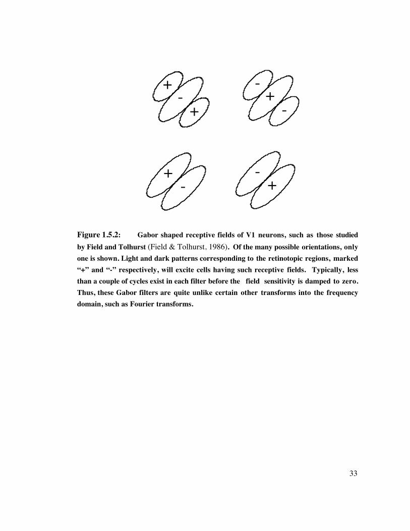
Figure 1.5.2: Gabor shaped receptive fields of V1 neurons, such as those studiedby Field and Tolhurst (Field & Tolhurst, 1986). Of the many possible orientations, onlyone is shown. Light and dark patterns corresponding to the retinotopic regions, marked“+” and “-” respectively, will excite cells having such receptive fields. Typically, lessthan a couple of cycles exist in each filter before the field sensitivity is damped to zero.Thus, these Gabor filters are quite unlike certain other transforms into the frequencydomain, such as Fourier transforms.

34

The are a number of connections between V1 layers. From 4Ca, M projections go

next to 4B, and P projections go to layers 2 and 3. 4B also projects to 2 & 3, as do

interlaminar regions of LGN. In layers 2 & 3, the response properties change again.

Along with the neurons having simple cell response properties, there are now the so called

complex cells. Complex cells are similar to simple cells except that they are not as

retinotopically specific. In other words, complex cells will respond to a simple cell type

stimulus, but unlike simple cells, they are tolerant to small translations of the stimulus

pattern.

Complex cells respond best to moving stimuli, and will also respond somewhat to a

flashed stimulus. Many of them are sensitive to the direction of movement as well. A final

property found in some complex cells of layers 2 and 3 as well as the simple cells of layer

4B, is that of end stopping (Gilbert, 1977). An end stopped cell is sensitive to the length of

the stimulus and actually responds less as the edge stimulus exceeds its preferred length.

Like so many other neuronal response properties, end stopping occurs to various degrees.

There are cells which are not end stopped, slightly end stopped, and completely end

stopped.

All the layer 2 & 3 neurons discussed so far have been orientation selective.

However, another class of center surround neuron is also found in these layers. These

center surround neurons are concentrated in cytochrome oxydase stained blobs which are

about .2mm in diameter (Wong-Riley, 1979). In addition to inputs from layer 4Cb, it is

the blobs which receive inputs directly from interlaminar neurons of the LGN. Livingstone

and Huble (Livingstone & Huble, 1984) determined that the blob neurons define a color

coordinate system. Each cell has what is called a double opponent property. A double

opponent cell has an excitatory center for a particular color, and it also has an inhibitory

center for the complementary color. The surround has a sensitivity to the same two colors,

but excitation and inhibition is reversed. Opponent color pairs are red-green, blue-yellow,

and black-white. Together, these three pairs form a three dimensional color coordinate

system which spans the same space as the original red, green, blue which is found at the

35

level of the cones. However, with the color opponent system also comes the basis for color

contrast and color constancy.

Blob and interblob neurons can be further compared according to the percent

which respond to color and in terms of spatial frequency. Although, color sensitivity is

usually thought of as residing in the blob neurons, some interblob neurons possess color

sensitivity in addition to edge orientation sensitivity (Lennie, 1990). In terms of spatial

frequency, blob cells prefer low spatial frequencies as compared to interblob cells which

respond to higher spatial frequencies.

From layers 2 & 3, the now well digested edge information flows down

reciprocated projections to layer 5, which in turn projects to layer 6. Layer 6 then

completes a loop by projecting back to layer 4. This loop demonstrates that the

phenomenon of descending pathways exists, not only between larger regions of cortex and

thalamus, but also exists between layers of a single region.

Both layers 5 and 6 contain complex cells, but their response properties differ

from those of layers 2 & 3. Each layer seems to have a particular shape to its neuron’s

receptive fields. Layer 2 & 3 neurons tend to respond more strongly as the edge length

increases. although some cells are end stopped. In layer 5, although the receptive field of

these neurons tends to be large, they do not increase their response as edge length

increases. In layer 6 the longer the edge is, the better the response.

Not all of the connections within V1 are vertical. There are pyramidal neurons in

the upper layers which have dendritic arbors that extend over 21mm, and axons which

have a lateral spread exceeding 4mm (Gilbert, 1992). Obviously, such neurons can

integrate information over a large portion of the visual field. This portion is larger than

what is normally considered to be the receptive field of V1 neurons. What then is the

function of these lateral connections?

36

Close inspection of lateral axon branching patterns, shows that they tend to

terminate in a number of discrete clusters. The relationship between neurons in terminal

clusters was shown in a number of ways. Pairs of neurons, one in each of two clusters,

were selected and a cross correlational analysis of their firing patterns was performed

(Ts'o & Gilbert, 1988; Ts'o, Gilbert, & Wiesel, 1986). It was found that neurons with

correlated firing patterns had similar orientations.

In another study (Gilbert & Wiesel, 1989), the registration of axon terminal

clusters to orientation columns was revealed by labeling the orientation columns with 2-

deoxy-glucose and labeling the horizontal connections with extracellularly applied tracers.

In a third study, a small 0.5 degree long light bar was used as a stimulus. The

response to the stimulus was then measured in two ways. One method used optical

recording, which reveals neural activity at the surface of the cortex. The other method of

response measurement used standard extracellular electrodes to monitor action potentials

(Das & Gilbert, 1995; Grinvald, Lieke, Frostig, & Hildesheim, 1994). Surprisingly, the

active optical area was larger than the active spiking area. The optically active area was 4

degrees in diameter whereas the spiking area was only 0.5 degrees, which was the size of

the stimulus and also the size of the typical receptive field size for that portion of the

retina. One explanation for this result is that the typical receptive field is the area which

exceeds action potential threshold, whereas the photoactive area contained neurons which

were either depolarized to a voltage below threshold or were hyperpolarized. Placing a

second light bar in various positions around the first light bar, showed that the surrounding

photoactive area was inhibitory, indicating that the neighboring orientation sensitive

neurons had been depolarized by the first bar. These inhibited neighbors turned out to

have the same orientation as the central neuron, which is consistent with the previously

described correlation experiment.

Based on this last experiment, one might conclude that these lateral projections are

inhibitory. Further studies, however, have shown that the connections are both excitatory

and inhibitory. McGuire et al. (McGuire, Gilbert, Rivlin, & Wiesel, 1991) have shown

37

that 80% of horizontal connections are to other pyramidal neuron and 20% are to

inhibitory interneurons. These excitatory and inhibitory connections work together as

follows: When the presynaptic pyramidal neuron is weakly activated, the total postsynaptic

response is excitatory, whereas, if the presynaptic neuron is strongly activated, the total

post synaptic response is inhibitory(Hirsch & Gilbert, 1991). The structure of this lateral

network will have important implications for experiments 1 and 3 of this thesis.

Yet another property of V1 neurons is ocular dominance, which refers to a cell’s

response bias towards one eye vs. the other. Ocular dominance is a feature of V1 neurons

at all layers, with the preference being more absolute in layer 4, whereas the preference is

more graded in the upper layers. Neurons with left and right eye preferences are

segregated into ocular dominance columns, which are actually slabs. Ocular dominance is

a precursor to disparity sensitivity, which is the neuron’s sensitivity to the distance the

object is from the animal. This measure is, of course, relative and it depends on the

alignment of the eyes at any given moment. Disparity sensitive neurons have been found

to be rare in V1 of monkeys (Poggio & Fischer, 1977); these cells are more common in

V2.

V1 outputs from all layers except 4C. Layers 2 & 3 project to other cortical areas

(V2, V4, and MT); layer 5 projects to the superior colliculus, pulvinar and pons; and layer

6 projects to the LGN and claustrum.

1.5.4 V2Like V1, V2 shows a regular pattern when stained with cytochrome oxidase.

Rather than showing an array of blobs, however, the staining of V2 reveals a pattern of

stripes. There are three types of stripes: thick, thin and pale. The thick stripes receive

input from V1 4B, the thin stripes receive input from V1 layers 2 & 3 blob neurons, and

the V2 pale stripes receive input from V1 layers 2 & 3 interblob neurons. Based on these

inputs, it would be reasonable to assign the role of motion analysis to the thick stripes, to

assign the role of color analysis to the thin stripes, and to assign the role of form analysis

38

to the pale stripes. In fact, some investigators have made this assignment (DeYoe & VanEssen, 1985; Hubel & Livingstone, 1987).

However, in a recent study, Gegenfurtner et al. (Gegenfurtner, Kiper, &Fenstemaker, 1996) have shown that the response properties of neurons in these stripes are

mixed. This is not surprising, because mixtures of neurons with different response

properties seem to be the rule in visual cortex. Gegenfurtner classified each cell according

to its sensitivity to direction of motion, orientation, color, and end stop. Each cell was

classified as sensitive to each of these properties or not sensitive to each of these properties.

Depending on how strictly he defined “sensitive”, he got different results. For medium

and weak sensitivity criteria, there were cells in each stripe type which met the criteria for

each of the four property types. Across the different criteria for sensitivity only a couple

of trends were consistent. One consistent result was that end stop cells were at least twice as

likely to be found in pale stripes than in other stripes. The other trend was that neurons in

thin stripes were less likely to be orientation selective than cells form the other two stripe

types. However, this second tendency was not very pronounced.

The exact function of V2 is not known. Most of the response properties of V2

neurons mentioned so far are the same as those studied in V1. It would be strange if V2

merely resorted the same information which was already calculated by V1. One possible

role for V2 would be to act as the first level of processing to produce surface information.

Supporting this conjecture is the work of Peterhans and von der Heydt which shows that

V2 neurons respond to illusory contours (Peterhans & von der Heydt, 1986; Peterhans &von der Heydt, 1989; von der Heydt & Peterhans, 1989a; von der Heydt & Peterhans,1989b; von der Heydt, Peterhans, & Baumgartner, 1984). About one-third of V2

neurons were found to respond to illusory contours. Whereas V1 monkey neurons are not

found to respond to illusory contours (von der Heydt et al., 1984), in the cat, some V1

neurons do respond to illusory contours (Redies, Crook, & Creutzfeldt, 1986).

Projections form V2 are sent to V3 (if it exists), V4, posterior inferior temporal

(IT), and MT.

39

1.5.5 V3V3 is normally considered to be part of the ventral processing stream. However, in

a recent review Kaas points out certain problems with the definition, and even the existence

of this area (Kaas, 1995). V3 was originally defined according to input patterns from V1,

and the existence of such patterns have more recently been supported by Shipp et al

(Shipp, Watson, Fracowiak, & Zeki, 1995). However, significant differences between the

ventral and dorsal halves of V3; such as connection patterns, architectronics, and neuronal

response properties have led some investigators to consider V3 to be two separate areas,

namely V3d and VP (Sereno et al., 1995). This new definition of the V3 area(s?) has a

problem of its own. Namely, the retinotopic map of V3d includes only the lower visual

field and Kaas finds this to be improbable. As improbable as it seems, there does exist

psychophysical evidence for asymmetry between the upper and lower visual fields. For

instance, Rubin et al. have found enhanced perception of illusory contours in the lower

visual fields (Rubin, Nakayama, & Shapley, 1996).

Another scheme for the organization of part the original V3 territory comes from

studies of new world monkeys (Krubitzer & Kaas, 1995). In this scheme, part of V3d is

joined with neighboring cortex to form an area called dorsomedial cortex (DM). DM

would then represent both upper and lower visual fields.

In summary, V3 appears to an area under continuing study and redefinition. In

spite of this, the general area called V3 has been shown to connect with other better

defined areas. Therefore, in the following sections, it may be referred to with respect to this

connectivity.

1.5.6 V4V4 covers an area from the anterior bank of the lunate sulcus to the prelunate

gyrus. Its inputs come from a variety of sources: V1, V2, V3, and MT, making it a fertile

region for some integrative process. V4’s input from V1 is small in comparison with its

40

major input which comes from V3, the thin stripes of V2, and the pale stripes of V2. With

such a variety of inputs, it is not surprising that V4 contains neurons which are sensitive to

direction of motion and orientation (Desimone, Schein, Moran, & Ungerleider, 1985),and color (Zeki, 1973).

The response properties of V4 neurons appear to be similar to those of V1

complex cells except that they respond to stimuli over a region four to six times the size of

a comparable V1 region (Desimone et al., 1985). Such an increase in receptive field size

is consistent with the notion that translation invariance is more pronounced in V4. Since

V4 is often thought of as a color processing area, one might also expect some sort of

higher level color representations there as well. Color constancy is one such phenomenon.

In fact, Zeki (Zeki, 1983) did find that the response of V4 neurons to color depends on

the colors in surrounding regions. He also found that these effects correlated with those

found in human observers.

In addition to color processing, V4 also performs important form related

processing. Lesions of V4 produce severe deficits in perception of form as well as deficits

in color discrimination tasks (Heywood & Cowey, 1987). This is consistent with the facts

that lesions of IT also produce deficits of object recognition (Mishkin, 1982) and that V4

has major projections into IT.

Activity of V4 neurons can be modulated by saccadic eye movements and other

attentional phenomena, providing further support for the idea that V4 is an integrative or

multifunctional area. Fisher and Boch have modulated the activity of V4 neurons using

several different saccade tasks (Fischer & Boch, 1981a; Fischer & Boch, 1981b; Fisher& Boch, 1983; Fisher & Boch, 1985); and Moran and Desimone showed that some V4

neurons distinguish between attended and unattended stimuli (Moran & Desimone,1985). Furthermore, using another form of attentional control, Haenny et al. found that

cueing could also modulate the response of V4 neurons (Haenny, Maunsell, & Schiller,1988). A cueing task is one where the animal is presented with a stimulus called the cue,

41

and then the animal is presented with a sequence of other stimuli, one of which matches

the cue. The animal’s goal is to respond to the matching stimuli.

In another cueing experiment, Ferrera et al. studied V4 responses to direction of

motion (Ferrera, Kirsten, & Maunsell, 1994). In this study, it was found that 33% of the

sampled neurons had a significant sensitivity to motion direction, whereas 24% had a

significant sensitivity to the cue direction after the cue was no longer present. Cue

sensitive neurons are interesting because they appear to encode short term visual memory.

Short term memory capability, in visual cortex, will be prove to be relevant in the

interpretation of experiment 3.

V1 and V2 have their homologues in the human brain. Therefore, one might

expect that V4 also has a homologue in the human, and that the macaque therefore

provides a good model for the higher visual structures of humans. Unfortunately, this

does not appear to be the case. The area of the human cortex most often associated with

color perception includes the posterior fusiform gyrus, as well as the lateral portion of the

lingual gyrus (Allison, McCarthy, Nobre, Puce, & Belger, 1994; Corbetta, Miezen,Dobmeyer, Shulman, & Petersen, 1991; Gulyas & Roland, 1991; Zeki et al., 1991), and

this region has been identified as a candidate for the V4 homologue. However, there are a

number of differences between V4 and the posterior fusiform gyrus. As already

mentioned, V4 neurons are known to respond to form related stimuli. In humans, PET

studies of form processing in posterior fusiform gyrus have yielded inconsistent results

(Corbetta et al., 1991; Gulyas & Roland, 1991). The most convincing evidence against

the posterior fusiform gyrus - V4 equivalence comes from lesion studies. Lesions of V4

do not produce the degree of color impairment that is found in humans with

achromatopsia (Heywood & Cowey, 1987) (Heywood, Wilson, & Cowey, 1987)(Heywood, Gadotti, & Cowey, 1992; Shiller & Lee, 1991). Finally, the location of V4 is

far removed from that of posterior fusiform gyrus, making the comparison weaker yet.

In general, one should not be surprised that a comparison of the design of the

monkey’s brain, with that of the human, should brake down at some point. The macaque

42

neocortex is about 9940 mm2 in area, 5467 mm2 of which is visual or visual association

cortex (Felleman & Van Essen, 1991). By comparison, the human neocortex has an area

of 142129 mm2 , which is large enough to dwarf the macaque brain (Shepherd, 1990).Natural, or even man made designs, being what they are, rarely scale in size without some

change in organization; even though the intended function remains much the same.

Therefore, it is only logical that there should be significant differences between the

organization of the macaque brain and the organization of the human brain.

1.5.7 MTThe middle temporal region, or MT is located in the lateral bank and floor of the

caudal superior temporal sulcus of the macaque and in the middle part of the temporal

lobe in New World monkeys. Aside from the usual means of region definition, such as

retinotopic patterns, connectivity to other areas and such; MT is can also be mapped as a

region of heavily mylinated neurons (Allman & Kaas, 1971; Ungerleider & Mishkin,1979). MT receives inputs from V1, V2, V3, V4, subcortical structures, such as the

superior colliculus and pulvinar, as well as descending inputs from ventral intraparietal

(VIP) and medial superior temporal (MST).

The neurons of MT are typically responsive to motion stimuli (Zeki, 1974). MT

cells receive much of their inputs from magnocellular origins and, consistent with these

origins, they are sensitive to low contrast and insensitive to color.

The directionally sensitive neurons of MT differ form those of V1. V1 neurons

are vulnerable to the aperture effect; where directionally sensitive neurons tend to assume

that motion is in a direction perpendicular to the orientation of the local edge element.

This problem arises computationally, when only local information in taken into account.

In contrast, a percentage of MT neurons are more sophisticated, in that, they use more

global information to deduce the motion of entire patterns (Movshon, Adelson, Gizzi, &Newsome, 1985). In addition to directional sensitivity, certain MT neurons are sensitive to

43

velocity (Maunsell & Van Essen, 1983) and others are sensitive to rotation (Saito et al.,1986).

Although MT is primarily a motion processing region, rather than a shape

processing region, there is at least one circumstance where MT contributes to the

recognition of objects. Marcar and Cowey have shown that lesions of MT interfere with

the recognition of objects which are defined by motion (Marcar & Cowey, 1992).

In humans, PET studies have revealed a region, known as V5, in the ascending

limb of the inferior temporal sulcus, which is activated by motion related tasks (Watson etal., 1993). A heavily mylinated zone, has also been found in approximately this same

position (Clarke & Miklossy, 1990), leading to the hypothesis that this is the human

homologue of MT. However, some uncertainty remains, because there are other regions

of the macaque brain which are both motion sensitive and heavily mylinated. MST is one

such area. The human region, referred to as V5, may actually be a homologue of one of

these other macaque regions.

1.5.8 ITThe inferior temporal region, or IT, receives input from V2, V3, V4, and MT; and

also projects back to these regions. IT covers an area of the temporal cortex from a point

just anterior to the inferior occipital sulcus to a point just posterior to the temporal pole,

and in the perpendicular direction, from the base of the superior temporal sulcus to the

base of the occipito-temporal sulcus. The scheme for subdividing IT varies according to

investigator. For instance, certain authors (Iwai & Mishkin, 1969; Von Bonin & Bailey,1947; Von Bonin & Bailey, 1950) have divided IT into two parts, TE and TEO; where TE

is the anterior portion and TEO is the posterior portion. TEO covers a region bounded by

the superior temporal sulcus, a point just medial of the occipito-temporal sulcus, and a

point near the lip of the ascending portion of the inferior occipital sulcus. Area TE

extends from the TEO to the sphenoid. TE and TEO are defined by means of lesion

studies and cytoarchitectonics (Iwai, 1978; Iwai, 1981; Iwai, 1985). In the lesion studies,

44

TEO lesions led to simple pattern deficits whereas TE lesions led to associative and visual

memory deficits. TEO and TE can also be distinguished by differences in the receptive

field sizes of their neurons. TEO neurons can have receptive field sizes as small as 1.5

degrees whereas TE neurons can have receptive field sizes of up to 50 degrees

(Boussaoud, Desimone, & Ungerleider, 1991; Tanaka, 1993). The inputs, which IT

receives from other areas, arrive in TEO, which in turn sends its output to TE. TE

reciprocates by sending back projections to TEO.

Felleman and Van Essen (Felleman & Van Essen, 1991) produced a different

scheme for subdividing IT. Their method was based on topography and the laminar

organization of projections. Using this approach they arrived at three subregions: PIT,

CIT and AIT, which are the posterior, central and anterior portions of IT respectively.

It has long been hypothesized, sometimes jokingly, that the process of object

recognition should culminate in a set of neurons, each of which responds to a particular

object. These are the so called “grandmother cells”, and they are referred to as such

because there would be one, for example, which would fire when you saw your

grandmother. The hypothesis of the existence of grandmother cells makes for one of the

simplest theories of visual object representation, because recognition of an object is

equivalent to the simple activation of a single neuron. More complex theories would

represent the recognition of an object as the activation of a set of neurons, as is often done

in artificial neural networks, or recognition may be represented by the synchronization of

firing patterns as proposed by Gray et al. (Gray, Konig, Engel, & Singer, 1989).

One of the fascinating discoveries about the response properties of IT neurons is

that grandmother cells actually do exist in IT. For example, Gross first showed that there

are neurons in IT which respond to hands, and other neurons which respond to faces

(Gross, 1972). Later, others showed that these responses were selective for the stimuli in

question (Desimone, Albright, Gross, & Bruce, 1984; Perrett, Rolls, & Caan, 1982).

45

However, one might still question whether IT represents the culmination of a

general object recognition process or, alternatively, IT might simply be a region where

faces and hands are recognized. One obviously would like to study a significant number

of different stimulus objects and their corresponding neurons. However, the

combinatorics of such a study could be daunting. Out of the seemingly limitless number

of objects which might be recognized by an animal, how can one hope to find those

neurons, out of the huge number of IT neurons, which respond to the selected test objects?

Logothetis et al. (Logothetis, Pauls, & Poggio, 1995) solved this problem by training

monkeys to recognize synthetic objects over an extended period of time. This training

method was successful in that approximately 12% of neurons tested were selective for

particular objects in the training set. The studied cells were from the upper bank of the

anterior medial temporal sulcus.

The various response properties of Logothetis’ experimental neurons show a

wealth of information about an object’s class, identity and position; all available in IT.

An animal must have information about certain objects at these different levels of

generality, in order to survive. For example, in order to fill in the properties of a new

instance of an object type, the classification of the object allows the animal to fill in the

new object’s characteristics via inheritance from the class. However, recognizing an

individual within a class can also be important, such as when the animal must recognize a

specific family or pack member. Furthermore, even though recognizing each scaled,

rotated or translated version of an object’s image as a distinct object would surely be

confusing, having positional information is sometimes essential when interacting with an

object.

Two types of object were used in the study, wire objects and amoeboid objects.

Certain neurons seemed to encode class in that they fired significantly more when

presented with one class member than when presented with a member of the other class.

Specific object neurons were also detected. These neurons responded to a specific object

but were invariant to viewpoint. Object neurons were somewhat rare as might be expected,

since only one such neuron is needed per object, although some redundancy would

46

certainly make the system more robust. A larger number of neurons were specific to a

combination of object and viewpoint. This also is to be expected since there are many

such combinations. The response of the object-viewpoint neurons varied in a smooth

manner as the view angle was varied from the optimal value. Thus object-viewpoint cells

are tolerant of small changes in viewpoint. The standard deviation of response curves was

approximately 29 degrees. This is important, since an infinite number of cells would

otherwise be required to cover all viewpoints. This characteristic of object-viewpoint

neurons held true whether the training was done with only static views of the objects or

whether the objects were rocked slightly about a training view. The effect, or lack of

effect, due to motion during learning will prove to be relevant to experiment 3.

Logothetis also tested neurons for translational, scale, and reflection invariance. All

of the cells tested for translational invariance were found to be somewhat sensitive to

position in that their response dropped off after less than 10 degrees translation. Scale

invariance was tested by varying the subtended angle from about 1 to 6 degrees. All tested

cells showed scale invariance within this range. As for reflection invariance, actually,

rotation about 180 degrees, or “pseudo reflection”, about 8% of all view selective cells

were found to have this property.

In a study by Leuchow, regarding translation and scale effects, it was found that

30% were translation invariant whereas 56% were scale invariant (Leuschow, Miller, &Desimone, 1994), Leuchow’s neurons were in the anterior ventral portion between the

anterior middle temporal and rhinal sulci.

Ito (Ito, Fujita, Tamura, & Tanaka, 1994) has also studied the response properties

of IT neurons. Ito’s neurons were in dorsolateral TE. He was interested in studying the

effects of contrast polarity on these neurons’ response properties. This is an interesting

question because , in some cases one would expect the contrast polarity of an object

model’s edges to be preserved in a viewed image, whereas in other cases one would expect

the contrast polarity to be reversed. For example, edges which are formed by

characteristic patterns of reflectance on an object, should always have the same contrast

47

polarity. For instance, birds and fish often have patterns which serve to identify them to

other animals, especially those of the same species, for purposes of mate selection, social

interaction, etc. Another case where contrast polarity is preserved is where shading in

caused by shape. Concavities tend to be dark and convexities appear light. When this

situation is reversed objects which are defined by such patterns are difficult to recognize.

However, there are situations where contrast polarity is not preserved. Suppose one

has an object which is medium gray in color. When this object is placed before a white

background, and then a black background, the polarity of the object’s border is reversed.

Such reversals occur frequently in the real world.

Based on the need to be both sensitive and insensitive to contrast polarity, one

would expect to find neurons of both types in visual cortex. In fact this is exactly what Ito

does find. However, it is yet to be determined whether these two classes of neurons

respond separately to object interior edge phenomena versus object boundary phenomena,

as one would expect. Contrast polarity is studied as part of experiment 1.

IT cells are not merely sensitive to the visual patterns which are presented to them.

Their responses can also be modulated by stimuli which have been presented a short time

before. These previous presentations, or cues, are part of the often used experimental

paradigm called delayed matching to sample (DMS). In delayed matching to sample, the

subject is presented with the cue object, then, perhaps after being presented with some

distractor objects, or perhaps after a simple delay, the cue object reappears and is selected

by the subject.

In the previously mentioned Lueschow experiment (Leuschow et al., 1994), ITneurons were monitored while macaques performed a DMS task. Leuschow found an

inhibitory cueing effect. In other words, a neuron which responded to the cue stimuli,

responded less vigorously when a matching stimulus appeared after some intervening

distractors. This decrease in responsiveness is consistent with Barlow’s (Barlow, 1990)ideas on perception, which will be discussed in a subsequent section. Leuchow et al. refer

48

to this effect as “adaptive mnemonic filtering”. Adaptive mnemonic filtering may be

responsible for some of the searching phenomena observed in experiment 2.

The higher processing level of IT, namely TE, projects to numerous areas, such as

TH and TF of the parahippacampal gyrus, STP, frontal eye fields, area 46, the amygdaloid

complex, and the hippocampus ( see the reviews of Logothetis and Sheinberg (Logothetis& Sheinberg, 1996) as well as Miyashita (Miyashita, 1993) ). The hippocampus is well

known as a region which is important to consolidation of short term memory. TE also

connects to other short term memory centers such as entorhinal and perirhinal cortices;

although the connection to the entorhinal cortex is made indirectly, via the perirhinal and

parahippocampal cortices.

The significance of the rhinal cortices to visual short term memory was

demonstrated by Meunier et al. (Meunier, Bachevalier, Mishkin, & Murray, 1993) and

Eacott et al. (Eacott, Gaffan, & Murray, 1994). Specifically, Meunier et al. showed that

ablations of rhinal cortex, especially perirhinal cortex, produced deficits in a delayed non-

matching to sample task. The non-matching version of the DMS task is similar to the

DMS task except that the subject is trained to respond to a non-matching stimulus rather

than one which matches the cue. Subsequently, Eacott et al. found that rhinal ablations

affected the DMS task performance only when the cue was unfamiliar. This later result

indicates that the rhinal cortex’s role is specific to short term visual memory rather than

visual memory in general. I will return to the role of short term visual memory in the

discussion of experiment 3.

It is not known for certain whether there is an exact human equivalent to the IT

region of the macaque. Nevertheless, human lesion studies have implicated the occipito-

temporal processing stream in the recognition of faces, animals, and other objects

(Damasio, Tranel, & Damasio, 1989; Farah, 1990; Levine, Warach, & Farah, 1985).However, lesion studies do not provide precise location information for the functions

studied, because clinical lesions can vary unpredictably from one individual to another and

they tend to be somewhat diffuse. Therefore, investigators have relied on other techniques,

49

such as PET or electrodes placed on the cortical surface, to locate precise functional

regions.

In a PET study, Haxby et al. have shown that mid- and posterior-fusiform gyrus

regions are activated during a face matching task (Haxby et al., 1993; Haxby et al.,1991). In a related set of tasks; Sergent et al. found that gender matching activated the

posterior-fusiform gyrus; identification of unique individuals activated the mid-fusiform

gyrus; and retrieving detailed knowledge about the individual, activated the midtemporal

gyrus, the parahippocampal gyrus, and the temporal pole (Sergent, Ohta, & MacDonald,1992).

Using electrodes, planted on the surfaces of the brains of human epilepsy patients,

Allison et al. have localized regions involved with the perception of faces, words and

numbers . See Allison for a review (Allison et al., 1994). The recognition of faces

corresponded to a negative 200 mV potential having a 200msec latency from stimulus

onset and a 140msec latency from activation of V1. This potential, referred to as N200,

occurred bilaterally in portions of the fusiform and inferior temporal gyri. These portions

do not represent a large area which is face responsive in all patients. Rather, it is the union

of smaller face responsive regions from a number of patients. Thus, there is considerable

variation among individuals, indicating perhaps, some random aspect of the developmental

or visual learning process. Other face specific potentials, some positive and some negative

were also found in the temporal pole region. These occurred between 200 and 300msec.

The temporal pole potentials may be related to the semantic face neurons found in PET

studies. However, semantic aspects of the stimuli were not investigated in the surface

electrode studies.

Word specific N200 potentials were recorded from the same general region where

face N200s were found. These potentials occurred in response to any letter string, not just

meaningful words. Number specific N200s were also found in the fusiform gyrus.

50

The PET and surface electrode studies in human temporal lobe, parallel the single

cell studies in monkey IT; except that, the human studies measure the responses of clusters

of cells and these clusters respond to object classes rather than individual objects.

1.6 Theories of Visual Cortex, and Related TheoriesStudies of visual cortex provide us with individual facts regarding brain function.

However, all of these facts must eventually be brought together into a coherent whole

which reflects back on the data, by explaining it. Furthermore, the resulting theory should

serve as a means to make predictions about biological function and guide subsequent

research.

The ultimate flavor of such a theory is difficult to predict. On one hand, it may

have the compactness and power of a physical theory such as Newton’s Laws of Motion.

Such a physics-like theory would consist of very few principles, but it would explain a

tremendous body of phenomena. Alternatively, the theory of the visual cortex may turn

out not to be much of a theory at all. Suppose, for example, that the mammalian nervous

system turned out to be like the mammalian digestive system in nature. In this case, our

understanding of it would be less like a distillation into a few fundamental principles and

more like an engineering blueprint for a contraption which gets the job done. Nature does

not guarantee that scientists will always find aesthetic satisfaction.

Whatever the flavor, proposed theories must be evaluated on their merits. The

most obvious desirable property is that the theory be accurate in its explanation of

observed and predicted phenomena. Some theories have corresponding machine vision

implementations. If they do, then one can ask for the corresponding functional property,

namely that the system works, works well, and that it works like its biological counterparts.

The possibility of a machine vision implementation brings to light yet another

desirable property of a given theory: a theory should strike at the crux of the vision

problem. There are basically two ways in which a theory might fail to satisfy this

51

requirement. It may be overly vague, thus making few concrete predictions which can be

tested; or it may explain how an easy part of the vision problem is solved while assuming

that the difficult part of the vision problem is somehow already solved. One way to test a

theory in this regard is to attempt to build a working machine vision system from it,

taking care not to introduce additional principles.

Finally, given two theories which are equal in all other respects, one should choose

the one which best satisfies the principle of Occam’s Razor. The classical example of this

is in the battle between the Ptolemaic model of the Solar System and the Copernican

model. When augmented with a complex system of epicycles, the Ptolemaic system

predicted the positions of the planets fairly well. Yet, the Copernican system eventually

won out by virtue of its simplicity. Occam’s razor would also choose a physics-like theory

over an engineering blueprint theory, should such a pair of theories contend for the role

of the true theory of visual cortex.

The following theoretical domains will be discussed: Bayes, which is a general

framework for modeling perception; minimum description length, a theory of

communication applied to perception; redundancy reduction, a general theory of

perception, binding exclusion, a theory of vision which is inspired by cortical attributes

and the properties of images but which may be generalized to other forms of perception;

and bidirectional models which are distinct models of the visual cortex and its internal

connections. All of these theoretical ideas serve as a springboard for a theory of visual

perception which is connectionist in flavor and based on the properties of images

themselves. This theory is presented in section 1.6.8. The theory, in turn, acts as the basis

for my experimental hypotheses.

1.6.1 Bayesian InferenceA perceiving animal or machine in its environment can be characterized as shown

in Figure 1.6.1. The visual world consists of a set of states or scenes, one of which is

presented to the vision system at a time. Information about the current world state is

52

made available to the vision system via the process of image formation. Obviously,

complete and untransformed information about the world cannot be transmitted to the

vision system, since this would require the world itself, or at least a neighborhood, to be

transmitted into the vision system. Perhaps this is what certain young animals are

attempting to do when they explore their environment by ingesting various portions of it.

In general, however, this is not a good idea; thus the need for image formation. Although

image formation is an efficient means for gathering information about the world, it does

have some disadvantages. Some information is lost, as would be expected by any process

which transforms a 3D representation into a 2D representation. Other losses in signal

quality are generally attributed to “noise”, as indicated in the figure. However, in the

present thesis, the cause of loss in signal quality is more specifically object incompleteness

and background.

53

The World Vision System

Si

Image Formation

Image Space

Model Selection

Noise

Model Space

SjSk

Mk

Mj

Mi

Mi

I

Figure 1.6.1: External and internal visual spaces.

Previously, theories of Bayesian inference have treated the process of perception as

a form of communication (Knill, Kersten, & Yuille, 1995b). However, the current

treatment, and Figure 1.6.1, presents perception as an interaction between states {Si} of the

external world and models {Mi}, internal to the vision system. This reformulation will

facilitate the subsequent comparison of Bayesian theories to other theories of vision.

Any particular instance of a perceptual system, in the Bayesian framework,

requires the specification of four basic components, as follows:

1) The elements of interest in the world states - In the case of visual systems, these are the

scene properties which the visual system attempts to detect or measure. The selection of

interesting elements are determined by both the nature of the world as well as the interests

of the system. Surface properties are examples of elements which are frequently of

interest, irrespective of the system’s specific interests. This is because surfaces define the

boundaries of objects and because surfaces are more likely to be visible than the interiors

of solids. In addition to universally interesting phenomena such as surface properties,

54

there are priorities which vary from system to system. Each system or animal has, for

example, distinct sets of objects which it may want to seek or avoid.

2) The structure of the set of world states - The world has certain regularities which allow

a system to interpret the data it receives. These regularities can be exploited by the system

to overcome ambiguities which are an inherent part of the data.

3) World state encoding scheme - In the case of vision, encoding occurs as image

formation. The details of the image formation process are in turn governed by the laws of

optics. In some Bayesian analyses, image formation and early image processing is skipped

and the analysis jumps directly to higher levels of processing.

4) Form of signal corruption - Noise is added to the representation of features at one or

more level of processing. A simple example of such noise would be Gaussian noise added

to pixel intensity values.

These specifics determine the information delivered to the seeing organism and must also

be incorporated into the seeing organism so that it can decode the signal.

The goal of a Bayesian system is to calculate the posterior conditional probability

distribution which is the probability distribution of possible world states given a particular

image:

p( S | I ).

(1) above is used to define the domain of S.

(2) is used to define the prior probability distribution p( S ).

(3) a model of image formation p( S ) = I in the ideal case.

(4) Actually, since the image formation may involve noise, therefore p( S ) + N = I

To calculate the posterior one can use Bayes’ rule of conditional probability:

p( S | I ) = p( I | S ) p( S ) / p(I ) (1.6.1.1)

55

but since p(I ) is constant for a given image we can try to find the S which maximizes

p( S | I ) = k p( I | S ) p( S ) (1.6.1.2)

This rule for selecting S is called the Maximum A-Posteriori, or MAP estimation. Otherpossibilities, such as selection of the mean of the distribution, or the Minimum MeanSquared-Error (MMSE) can also be pursued.

Calculating the likelihood function p( I | S ) depends on an understanding ofimage noise as well as an understanding of how images are formed from world states orscenes. Candidate scenes have non-zero probability. One way to characterize a typicallikelihood distribution is to note that for a given image, p( I | S ) is zero almost everywhere. In other words, while there may be an infinity of scenes which can produce aparticular image, still this is a tiny fraction of all possible scenes. A good example of theway the likelihood constrains the space of all scenes is found in the work of Sinha andAdelson (Sinha & Adelson, 1993) 2. In their paper, they show how one might compute 3Dpolyhedrons, from 2D image projections. As shown in Figure 1.6.2, a given projection ofa wireframe polyhedron can be generated by an infinite number of 3D wireframes.

2 Although a Bayesian framework would be suitable for this paper of Sinha and Adelson, they do notactually use the terminology of Bayesian analysis.

56

Figure 1.6.2: Any number of 3D wireframes can project onto the same image. Some

are preferable to others. Adapted from Sinha and Adelson (Sinha & Adelson, 1993).

57

In spite of these many possible world states, the set of all possible world causes for the

projected image is a small subspace of all polyhedrons. Thus, the set of non-zero

posterior probabilities is significantly reduced, according to Bayes’ rule or equation

1.6.1.2.

Intuitively, one can see that not all wireframe shapes in 3-space are equally likely.

In order to further reduce the set of possible causes for the image, one must next turn to

the prior distribution, which tells us which 3D forms are most probable, independent of

image formation. Sinha and Adelson impose a prior-like criteria for the probability of

various wireframe shapes. Their criteria requires that the 3D shapes optimize 3 measures;

one which attempts to minimize angle variance, one which attempts to maximize the

planarity of faces, and one which seeks to maximize compactness. Such a criteria favors

polyhedrons such as the lowest one in the figure.

Finally, now that a likelihood and a prior distribution can be defined, the task of

determining the proper wireframe requires that a maximum for equation 1.6.1.2, or MAP

estimation, be found. If the posterior distribution was differentiable, and the zeros of the

derivative could be determined directly, then one could produce a closed form solution for

the maximum. However, this is almost never the case. Thus, a numerical method such as

gradient ascent is usually employed. In other cases, there are no obvious means for

quantitatively formulating the prior or the likelihood, and the Bayesian analysis does not

lead directly to algorithmic development.

In addition to acting as a framework for developing machine vision algorithms,

Bayesian analysis is useful to psychophysicists when studying human perception. By

definition, psychophysics observes the brain as a black box. The psychophysicist knows

the input and the output of the black box but does not know the algorithm which is

running inside that box. However, one can guess at the algorithm and then compare the

performance of the black box to the performance of the algorithm. Bayesian analysis

provides a concept, called the ideal observer, which provides a means for making such

comparisons.

58

An ideal observer is a hypothetical observer which makes the best choice in a

statistically defined problem, given the information available. The formation of an ideal

observer places an upper limit on the performance of a human subject. If this limit is

exceeded during an experiment, one can deduce that some assumptions about the model

for the distribution p(S | I) are in error. If p( S | I ) is in fact the same as that used by the

human, then the real human becomes ideal. This possibility is maintained by the strong

view of Bayesian perception. In the strong view, a complete functional characterization of

human perception consists of a Bayesian description of the world and a specification of

the tasks which humans perform. If, on the other hand, one maintains that the

performance and efficiency of the human observer also depends on the manner in which

the algorithm is modularized internally, then one is assuming the weak view of Bayesian

perception.

Aside from recognizing that the Bayesian view made need to be expanded, and to

account for the effects of algorithmic implementation, other refinements are desirable. So

far, it has been assumed that the ultimate goal of any organism is to accurately interpret its

environment. However, while a tendency towards accurate interpretation should generally

be useful, the ultimate goal is likely to be something else. For example, from an

evolutionary point of view, the goal of any organism is to pass its genes to the subsequent

generation. Such a goal has many immediate subgoals, such as finding a mate, and

avoiding starvation and predation in the meantime. To account for these other goals, a

loss function must be specified. The loss function estimates the cost of various decisions

for particular organisms or systems (Yuille & Bulthoff, 1993). Or as stated by Yuille and

Bulthoff, “The loss function emphasizes that the interpretation of the image cannot be

divorced from the purpose of the visual system.” An exact formulation of this idea is as

follows: Let {S} be the set of all possible scenes and let {d} be the set of all possible

decisions regarding scene identity. Then, in order to determine the behavior of the system,

one must define a loss function L(S,d) which returns loss L when the true scene is S and the

system decides that the perceived scene is d. By definition, the goal of any perceiving

system is to minimize its loss L(S,d). However, in any given situation, the system does not

59

know what the true scene S is, so it cannot directly minimize L(S,d). Instead, it has only

the image I, and perhaps an estimation of the probability p( S | I ). With this information

it can calculate the risk R of making any decision d, given image I

R d | I( ) = L S, d( )Ú p S | I( ) dS[ ] . 1.6.1.3

In this formulation, all possible scenes are considered as explanations for the image, but

each is weighted according to its probability.

Another enhancement to the Bayesian approach, which was also described by

Yuille and Bulthoff, is worth mentioning. This is the idea of competitive priors. In any

given situation, the optimal prior p( S ) will be determined by the task at hand. The task,

in turn, may be determined by non-visual considerations or by the contents of the scene.

In the case of non-visual considerations, such as the current behavior of the seeing animal,

say feeding or searching for a mate, the correct prior can be determined rather

unambiguously. However, in the case where the scene contents determine the task, one has

only the image as input to the prior selection process. For example, suppose that a scene

may contain a number of distinct shape types, such as spheres, cones, cylinders etc.

Further, suppose that one prior model p(S) and likelihood function p( I | S ) is well suited

to spheres (Pentland, 1989) while another prior and likelihood is tailored to cones and

cylinders (Woodham, 1981). Each model system will tend to outperform its rivals, given

scenes native to its geometry type, because that model system can exploit constraints

tailored to that particular geometry. In general then, one has a set of models { ( pi( S ) , p

i( I | S) ) } indexed by I, each suitable for a class of scenes. As in the case of loss function

analysis, we have only the image I as external input to our decision process, but now we

must make a decision d and choose a model i. Therefore, as before, one can take a

weighted average, but this time it is over both the set of all possible scenes and the set of all

models. Hence the risk function for competitive priors can be expressed as

R d, i | I( ) = p a( ) L S, a;d, i( )Ú pa S | I( ) dS[ ]a . 1.6.1.4

60

where a is the optimal model, p( a ) is the probability that a is the correct model, and

L(S,a,d,i) is the cost of deciding d for the scene using model I, when the true scene is S and

the best model is really a . By finding the scene and model which minimizes this risk

function, the system can determine the most likely scene. As in all applications of

Bayesian analysis, the challenge of producing a meaningful realization of equation

1.6.1.4, and the challenge of finding a minimum of the resulting expression, should not be

underestimated.

1.6.2 Bayesian Analysis in Psychophysics

In the present experiments of this thesis, image phenomena such as edges and

shading are generated by some unknown scene phenomena. However, the image data

which requires explanation may take other forms. For example, Knill et al. study the

possible scene causes of shadows in their stimuli (Knill, Kersten, & Mamassian, 1995a).In one experiment, they use an illusory stimulus which might be referred to as a looming

square. In this looming square illusion, a square is floating above a checkerboard

background and a shadow is cast by the square onto the checkerboard. See Figure 1.6.3.

The square is stationary in the image. Any movement of the shadow could be due to

motion of the light source or it could be due to the looming of the square towards the

observer. However, if the square is approaching the observer, the laws of perspective

image formation require that it should also increase in size in the image. Probabilisticly

then, the likelihood distribution p(I|S) has a mode, i.e. the graph of p(I|S) has a “hump”,

where S contains a forward moving square and I contains an image of the square which is

becoming larger. Correspondingly, p(I|S) is minimal at points where the square moves

toward the observer and the size of the square’s image does not increase. The probability

is low at these points because they violate the laws of image formation. In this analysis, the

scene and the image are not the usual snapshot, but, like a film scene, they have some

extent in time as well as space. If considered alone, the likelihood would tend to form a

minimum in the posterior probability p(S|I) where the square approaches the observer and

61

the square’s image does not increase in size. However, the prior also has an effect on the

posterior probability. Since the motion of the shadow must be accounted for by either the

motion of the light source or motion of the square, the prior will have a non zero value at

either or both of these points in scene space. Prior to the experiment, there is no way to be

certain of which set of points has the greater probability. However, from ecological

considerations it could be argued that natural light sources, such as the Sun and Moon,

move very slowly, thus appearing stationary to most animals.

62

Figure 1.6.3: Other than the shadows, both images are the same. The greensquare on the right seems to be floating above the blue checkerboard. From (Kersten,Mamassian, & Knill, 1997).

Figure 1.6.4: (b) and (c) are identical except for the shadows. The ball in ( c )appears to be floating while the ball in (b) appears to lie on the floor of the box. From(Knill et al., 1995a).

63

From the analysis so far, it is apparent that a likelihood, which favors an

explanation of a moving light source, would be in conflict with a prior which favors a

stationary light source. Hence, one must turn to the empirical evidence to determine which

distribution is dominant in its contribution to the posterior distribution, which ultimately

determines the observer’s interpretation of the image. As it turns out, human observers

tend to see the square in motion, indicating that there is a prior bias against light source

motion. The empirical results also show that this prior bias must dominate the effect of the

likelihood distribution.

In the same paper, Knill et al describe the ball in the box experiment. While the

analysis of the looming square is qualitative in nature, the ball in the box experiment

utilizes an ideal observer model to provide a quantitative measure of subject performance.

The experimental stimulus consists of a open box having a checkered floor and sides.

Furthermore, the box contains a ball which casts a shadow on the box floor. The light

source is a point source at infinity. See Figure 1.6.4. An ideal observer can be defined by

defining the likelihood and prior distributions, or equivalently, by identifying the

assumptions made by the ideal observer regarding image formation and the assumptions

made regarding the structure of the scenes.

In this analysis, it is assumed that the problems of recognizing the ball, recognizing

the shadow, and estimating their locations, are somehow already solved, so that the analysis

begins at a fairly high level. The model of image formation is therefore not explicit about

determining pixel values but rather is expressed in terms of object coordinates and angles.

Knill et al calculate a single parameter which is used to describe the image domain,

namely, the visual angle between the ball and the shadow, f, as a function of scene

parameters:

f = cot -1 dh

sin t L( )sin s L( )sin s S( ) + cos s L( )cos s S( )sin s L( )

- tan s L( )È

Î Í ˘

˚ ˙ ,

1.6.2.1

64

where h is the height of the ball above the planar surface, d is the distance between the ball

and the viewer, sL is the slant of the illuminant away from the viewer, tL is the tilt of the

illuminant relative to the horizontal in the image plane, and sS is the orientation of the

planar surface, expressed as the slant away from the viewing direction. Although this

equation is somewhat complex, the important point here, is that a precise description of

image formation has been given as a function of the scene parameters. In terms of

distributions, it may be said that the likelihood distribution will have a significant value

wherever equation 1.6.2.1 holds and will be near zero elsewhere.

In order to describe the prior scene knowledge of the ideal observer, some

description of physically possible and physically impossible scenes must be given. Or, to

phrase this in a more statistically fuzzy manner, one needs to describe which physical

scenes are more or less probable. Knill et al chose to have modes of probability in the

prior distribution where the box floor is planar and stationary, the ball is rigid and non-

expanding, and where the light source remains stationary. With regards to equation

1.6.2.1, this implies that all parameters remain constant except for d and h. d(t) and h(t)

as functions of time, describe the trajectory of the ball.

In the experiment, the image if the ball and the image of the shadow were moved

along straight trajectories, and the angle between these two trajectories was allowed to

change. The height of the ball, at the end of its trajectory, was then estimated by human

observers as well as the ideal observer. The ideal observer was able to calculate the height

according to

h = dsin tL( )sin s L( )sin sS( ) + cos s L( )cos sS( )

sin s L( ) tan f( ) + tan s L( )( ) , 1.6.2.2

which is derived from equation 1.6.2.1, while also taking into consideration the prior

constraints. The results showed that the human and ideal observers produced very similar

psychometric curves, indicating that the ideal observer was a good model for the human

65

observers. Thus one can conclude that human observers do indeed assume that the source

of illumination is stationary and that the human model of cast shadow image formation is

suitably expressed by equation 1.6.2.1.

In a variation on the previous approach Liu et al (Liu, Knill, & Kersten, 1995) do

not compare the psychometric curves of human and ideal observers; instead, they compare

the accuracy of a number of ideals3 with the accuracy of human observers. Because ideal

observers have no inefficiencies, any ideal which is out-performed by a human ideal can

be discounted as a possible model for the human observer. Also, assuming reasonable

efficiency on the part of the human observer, any ideal which grossly exceeds the

performance of a human, can also be discounted as a candidate for the correct human

model.

This model bracketing approach was used to study whether humans utilized 2D or

3D internal representations when recognizing objects. Small spheres, connected by thin

cylindrical sections, were used as objects to be learned and discriminated. A number of

these “bent paperclip” objects can be formed by random placement of the sphere-vertices

in 3-space. Human observers were trained to recognize these objects by viewing them

from a number of viewpoints. Later, the human subjects were tested in a discrimination

task. The two stimuli in the discrimination task each consisted of a prototype which was

rotated to some random position. The “learned object” then had noise added to its vertex

positions while the distractor had a probability of a greater amount of noise added to its

vertex positions. The task then, was to select the learned object over the distractor. Using

this method, it is most likely that the distractor will have a greater distortion than the

learned object; however, there will be times when this is not the case. One then expects the

ideal observer to make an “error” in classification.

3 Strictly speaking, there can only be one ideal observer per task. The ideal observer is the observerwith the most complete information available to execute the task. Other observers, with more limitedinformation, can be called sub-ideal observers; and observers with access to more information than isrealistic, might be called super-ideal. For the sake of simplicity, I will refer to all these observers asideal, and will specify the information available to each one. All these observers are free of algorithmicinefficiencies.

66

Liu et al formulate a number of ideal observers, of which, three will be mentioned

here. One ideal observer (sub-ideal) has a 2D stimulus representation and a 2D internal

model. This 2D/2D ideal stores all of the training views and compares each of these to the

image during recognition. For any image, the 2D/2D ideal can produce a measure

similarity between the image and any chosen internal model. It does this simply by

summing the errors of the vertex positions. One interesting aspect of this ideal is that it

treats rotational variance and noise in the same way, and has no knowledge of rotational

regularities.

The second ideal is one with a 2D stimulus and a 3D internal representation. The

similarity metric for this ideal is computed by rotating the internal representation until its

2D projection is most similar to the 2D image. The metric can then be measured as in the

2D/2D case.

The third ideal (a super-ideal) has both a 3D stimulus and a 3D internal

representation. This ideal has unrealistically complete information about the 3D

coordinates, since the experimental stimulus is 2D. The similarity measure is similar to

that of the 2D/2D observer except that it is computed on 3D coordinates.

Liu et al find that, for most object types (there are four types in the experiment),

the human observers outperform or match the performance of the 2D/2D ideal. Since the

human observer cannot outperform the ideal by means of algorithmic efficiency, the result

indicates that the 2D/2D ideal is not a suitable model for human perception. The most

obvious explanation for the 2D/2D ideal’s poor performance is the manner in which it

lumps together the variance due to noise and the variance due to rotation. The relatively

high level of human performance is evidence that the human observer, unlike the 2D/2D

ideal, does indeed recognize the inherent structure of rotational variance. This conclusion

is perhaps, the most interesting product of the study.

67

The efficiency of the 2D/3D and the 3D/3D ideals, relative to humans, was

consistently greater than 100%. Such efficiency measures leave these ideals in contention

as models for the human observer, although the formulation of the 3D/3D observer is

unrealistic. In general, the 2D/3D and 3D/3D results are more difficult to interpret than the

2D/2D results, because the algorithmic efficiency of the human observers is unknown.

1.6.3 Bayesian Models of PerceptionThe Bayesian approach can also be used to formulate models of biological and

machine vision systems. One example of this, is Freeman’s clever application of Bayesian

analysis to the problem of finding solutions to the shape from shading problem (Freeman,1994). In the shape from shading problem, the system is given an image of light intensity

values which have been produced by light, from a directional source, reflecting off of a

surface in 3-space. The problem, then, is to determine what surface shape might have

produced a given image. An interesting aspect of this problem is that, as in the case of

Sinha and Adelson mentioned earlier, there may be multiple scenes which can equally well

account for the image. Sinha and Adelson solved this problem by defining a prior

distribution which labeled some shapes as less likely than others.

In Freeman’s approach, all shapes have equal prior probability; therefore, some

other criteria must be used to distinguish among those shapes which can account for the

image. He begins by separating the scene parameters into those of interest and those not

of interest. In the present example, the shape of the surface is chosen to be of interest and

the direction of the illumination is selected to be not of interest. Freeman refers to those

parameters which are not interesting as generic variables.

Let b represent the shape variable, let x represent the light direction, and let y

represent the image. Since the scene can be broken into two variables, Bayes theorem

gives

68

p b, x | y( ) =p y | b, x( )p b( )p x( )

p y( )1.6.3.1

as the posterior probability. However, since x is the generic variable, one is reallyinterested in p( b | y ). Fortunately, x can be eliminated by integration

p b | y( ) =p b( )p y( )

p y | b, x( )p x( )xÚ dx 1.6.3.2

where p(y), p(x) and p(b) are all considered to be constants. Therefore, one only needs tomaximize

p y | b, x( )xÚ dx 1.6.3.3

over b . This can be estimated by counting, for each b, the number of discrete light

directions where the resulting image looks similar to y. Freeman demonstrates how this

method can simulate human interpretations of Ramachandran’s bumps (Ramachandran,1988) as well as human face surfaces. In both cases, there is the intuitively correct human

interpretation of these images, as well as a number of unexpected explanation surfaces.

However, each unexpected surface produces the image for a relatively small number of

lighting directions and is therefore given a low probability according to equation 1.6.3.2.

Freeman’s approach seems like a promising tool for machine vision researchers

and brain models. However, it should be noted that more work remains to be done before

this technique can be practically applied. The difficulty lies in the fact that the space of all

surfaces is huge and hence it is difficult to search. Therefore, some means of generating

candidate surfaces must be made available. In the given simulations, the “correct” answer

was included among the candidates, by the human experimenter. This was possible

because his own visual system had solved the surface recognition problem prior to the start

of the simulation. Any real machine vision system, or real brain, does not have a little

man, or homunculus, standing by to provide such hints.

69

In a somewhat more abstract analysis of model selection, MacKay, in his paper on

Bayesian interpolation, has divided the task of data interpretation into two levels (MacKay,1992). Suppose that one has a parametrization for scenes, which involves some n

parameters. MacKay refers to such a parametrization, when combined with a prior and

likelihood distributions, as a model. If there is only one such model then the only

perceptual task is to find the parameter values which best fit the given image data.

However, if multiple models exist, then the other level of data interpretation must also be

solved; namely, one must choose the best model.

Given a particular model Hi, and image data I4 , MacKay expresses the posterior

probability of a scene r S as

p

r S | I, Hi( ) =

p I |r S , Hi( )p

r S | Hi( )

p I | Hi( )1.6.3.4

which is the same as the usual definition of a posterior, except that all the distributions are

conditional on model Hi. He refers to the denominator p I | Hi( ) as the evidence.Intuitively, the motivation for this terminology is not apparent until one proceeds toMacKay’s second level of Bayesian inference.

The posterior for the model Hi is given as

p Hi | I( ) µ p I | Hi( )p Hi( ) . 1.6.3.5

This is also the usual formulation for a posterior, except that, without the normalizing

denominator, one has a proportionality rather than the original equality. The question to

be answered at this level of analysis is, “which model is the best model, given image data

I?” Since the left hand side of this proportionality is the probability of model Hi given

4 Actually, MacKay does not restrict his analysis to visual perception. Instead of images, he simply has“data”, and instead of a scene, he has a list of parameters which specify a real world state.

70

image I, the answer to our question must lie on the right side. The right side has two

factors. One is the prior factor p Hi( ) , which can be a relatively subjective measure ofhow good a model is. On the other hand, the likelihood p I | Hi( ) is not subjective.Therefore, the likelihood is the best objective measure that Hi is the correct model given

the data. This is why MacKay refers to this likelihood distribution as the evidence for Hi .

The next step in this analysis is to evaluate the evidence for a given Hi . To do this,

one must recognize that the probability of observing image I under model Hi , depends,

from moment to moment, upon the parameter settings r S . Therefore, one must consider

the effect of all possible parameter settings, as accomplished by the following integral

p I | Hi( ) = p I |

r S ,Hi( )p

r S | Hi( )

SÚ d

r S 1.6.3.6

This can be thought of as the convolution of functions p I |

r S ,H i( ) and

p

r S | Hi( ) , or it can

be thought of as an unnormalized correlation of p I |

r S ,H i( ) and

p

r S | Hi( ) , where

summation is by integration. Since MacKay’s focus is on interpolation, or curve fitting,it is appropriate that 1.6.3.6 deals with one image at a time. However, when modeling avisual environment, equation 1.6.3.6 would serve better it was generalized to take multipleimages into account, as in the following:

p E | Hi( ) = p I j | Hi( ) p I j |

r S ,Hi( )p

r S | Hi( )

SÚ d

r S

j =1

n

 1.6.3.7

where E is the visual environment consisting of n images and where each image has a

probability p I j | Hi( ) of occurring. Nevertheless, equation 1.6.3.6 is quite suitable for

illustrating the principle of evidence, and I will refer to it in the remainder of this section.

The correlation analogy for equation 1.6.3.6 is illustrated in Figure 1.6.5 throughFigure 1.6.11. In Figure 1.6.5, an arbitrary instance of the distribution

p I |

r S ,H( ) is

shown. For a given image I, peaks occur in this distribution at the most likely scenes. InFigure 1.6.6, Figure 1.6.8, and Figure 1.6.10, distributions

p

r S | H( ) are shown. There

71

are at least two ways that the model H can fail to be a good model. The model can failbecause its prior is out of alignment with the likelihood or the model can fail because it isto general. In Figure 1.6.8 the peaks of the distribution are offset from the peaks of thelikelihood distribution. Since the integral of equation 1.6.3.6 is essentially a correlationof the two distributions, the evidence will be high when the peaks of the two distributionsare aligned and low when the peaks are misaligned. In the case misaligned peaks, nomatter where the true scene parameters lie, either the scene is unlikely, or it is unlikelythat the scene could have formed the image. If images, such as I, occurred frequentlyenough, then the model would be forced to disagree with the empirical data. In particular,either a scene will prove itself to be common when the model says it is not, or an image-scene pair

I |

r S ( ) will occur frequently while the model claims that

r S is unlikely to cause

I.

Figure 1.6.5: An example likelihood distribution for some fixed image I andmodel Hi. The example is somewhat fanciful since a real scene space is unlikelyto be one dimensional.

72

Figure 1.6.6: An example prior probability distribution. The prior “agreeswith” the likelihood at at least one location, around S=5.

73

Figure 1.6.7: The product of the probability indicated the most likely scene,namely S=5. The integral of the distribution indicates the evidence for themodel Hi. That integral is approximately .071.

74

Figure 1.6.8: If the model is replaced by some other, say Hj, then the priordistribution will change as a result. The likelihood distribution may alsochange. However, for simplicity, let us assume that the likelihood distributionis the same throughout these examples. In the case of this model Hj, a problemarises due to the misalignment between the peaks in the likelihood distributionrelative to the prior distribution.

75

Figure 1.6.9: The product of the likelihood and the prior under the model Hj.Since the peaks don’t line up between these two distributions, the best scene isnot so obvious. Also, the evidence for the model Hj is now decreased to .0451.

If the prior probability of the scene is as in Figure 1.6.10, then the model againproduces a low measure of evidence. In the case of model Hk, the problem lies in thefact that the model takes into account a large number of scenes which are not representedin the image data. In other words, given the data, the degree of model complexity isunwarranted. That a model should not be unduly complex, is the well known principle ofOccam’s razor. Occam’s razor is often taken as intuitively correct, or as an axiomaticmeasure of the quality of a scientific theory. Here, Bayes provides objective justificationfor judging models according to Occam.

76

Figure 1.6.10: Yet another model, Hk, suffers from being too general. Note thelarge number of peaks in the prior distribution.

77

Figure 1.6.11: Once again, the best choice of scene is not so clear. The evidencefor the model Hk is approximately .0613.

78

1.6.4 Stochastic Complexity and Minimum DescriptionLength

Stochastic complexity and minimum description length (MDL) are information

theoretic notions which have formulations reminiscent of Bayes. In fact, it has even been

claimed that Bayes and the information theoretic approaches are “essentially equivalent”

(Mumford, 1995). However, the founder of stochastic complexity and MDL, Jorma

Rissanen, disagrees, stating that the comparison “has caused a lot of confusion about the

entire MDL principle” (Rissanen, 1997). The difference between the two approaches is

that, while Bayes begins with the intuitive and axiomatic idea that the goal of a perceiving

system should be to deduce the world state given some stimuli, the goal of a stochastic

complexity or MDL based system is to find the simplest explanation for the stimuli.

Although the motive for Rissanen’s ideas is not as intuitive as Bayes, there are famous

examples of “simpler is better” in science, where the search for truth in science serves as

an analogy for the search for a true interpretation by a perceiving system. Perhaps the

best known example is that of the contest between the Ptolemaic theory of the solar system

and the Copernican theory. While the accuracy of the Ptolemaic system was quite good, if

one added ever more epicycles to the orbits of the planets, the Copernican system could

make the same predictions with less complexity and so gained favor over the Ptolemaic

system. The difference between this example and Rissanen is that, in the solar system

example, the virtue of simplicity was applied as a kind of tie breaker, after all other criteria

have been applied to compare the two theories; whereas, Rissanen takes the bold step of

applying the measure of simplicity first and foremost. As we shall see, he justifies this by

showing that simplicity and accuracy are, in a sense, equivalent.

The idea of stochastic complexity has its roots in the work of Kolmogorov

(Kolmolgorov, 1965) who proposed that the best model of the “machinery” which

79

generated an observed data set, is the shortest computer program which could have

produced such a data set. The length of such a minimal program is called the Kolmogorov

complexity. Of course, in our case the data set is an image and in Bayesian terms, this

resulting computer program is analogous to a model for the scene S.

To intuitively understand the motivation for this approach to image interpretation,

consider the following example: Suppose the image to be represented is of a

checkerboard. One good model of the image would be a program consisting of four

nested loops. The innermost loop counts up to the width of a check, and at each count, it

writes out a white pixel to a sequence of column locations in a rectangular image buffer;

the row index is held constant. The next loop out increments the row index of the pixel

address for each count. The loop outside of that increments the lateral location of the

check origin and toggles the color for each count. Finally, the outermost loop increments

the vertical location of the check origin for each count. This program is not only a

compact way to represent the image, it also contains more accessible information than the

image itself. One could in fact use the raw image as the basis for an extreme example of

an image producing program. Let the program store all the pixel values as constants.

Then, when run, the program simply writes out the constant values to the appropriate pixel

locations. Such a program is not only internally redundant, storing the same checks over

and over, but none of structural information about the image, such as the check size or the

number of checks, is represented explicitly. Finally, any program written in the same

language as the four loop program, which is also significantly shorter than the four loop

program, will not be able to produce an accurate image of the checkerboard. Therefore,

the four loop program, which is the most compact yet accurate program for the

checkerboard is also optimal as an interpretation of the checkerboard image. The

unfortunate thing about Kolmogorov programs is that there is no known means of

producing one for images in general, and so this method of producing models of scenes

will probably remain fruitless.

In spite of the limitations of Kolmogorov, Rissanen believes that the idea of Occam

derived models is too good to abandon (Rissanen, 1997; Rissanen, 1996). Therefore, he

80

has sought a way to proceeded in this direction. One way to make this possible, is to give

up on finding an algorithm which will produce a program or model and to instead start

with a set of known models and to define a metric which selects among those models. One

such metric, he refers to as stochastic complexity.

In defining stochastic complexity one begins by specifying a set of models {M i}

to be evaluated. Each model M i has a vector of parameters q = (q1, q2, q3,..., qk) which fit

the model to a particular set of data. For instance, although such an example might be too

simple for many vision applications, one can think of the case where M i is a polynomial

with coefficients q,. For each model M i there is a likelihood distribution p( xn | q ) which

indicates the probability of the model producing image xn , when the parameters are set to

q. xn can be thought of as a pixel array or some higher level vector description of the

image. Rissanen finds that it is not necessary to restrict the distribution p( xn | q ) to being

a probability, but rather, it can be a distribution in a more general sense, and thus notated

as

f( xn | q ). However, for the sake of concreteness, it is still useful to think in terms of

probability.

Rissanen then proceeds to define stochastic complexity as the negative log of

ˆ f (xn) =f (xn | ˆ q (xn))

f (y n | ˆ q (yn))dy nynÚ

1.6.4.1

where ˆ q (xn ) are the parameter values which maximize the probability of producing xn,

and q is restricted to some range. The range of q should make the denominator finite.

Since the negative log function adds nothing useful to this formulation of stochastic

complexity, one can maximize 1.6.4.1 rather than minimize the stochastic complexity.

The numerator is akin to the likelihood of Bayesian analysis and so it is the same as the

posterior probability, except that there is no prior. The denominator provides the Occam

part of the measure, in that it penalizes any model which fits too many images yn.

81

So far this is rather abstract, so it might be illustrative to see how the concept can

be used as a theory of the object recognition process. Suppose that the brain contains a set

of models of objects M i. As discussed previously, there is good evidence for such object

models in region IT, and at lower levels of processing, there are models of more primitive

constructs such as edges. Now, when an image is transmitted to the visual cortex, it is

usually in a widely varying form. That is, every time a particular object appears, it

generates a different image xn, due to variations in lighting, translation, scale, orientation,

flexing of the object, articulation of the object, etc. Therefore, for the model to fit, one

must optimize over q. Thus one way of looking at the most probable q is to equate it with

the best fitting q. In general, one wants to chose the IT object model, for which a good

parameter fit can be found. However, this model choice must be qualified. To see why,

suppose that the model was suitable for any set of m curves. Such general curve fitting

models exist and are used in computer aided design, for example: non-uniform rational B-

splines (NURBS). When given an image, parameters can be found to fit all the edges in

the image. Yet, the NURBS “object” is a useless model since it accepts all images as

being a representation of that object. Therefore, it cannot be used to differentiate between

objects. The denominator of 1.6.4.1 prevents a model like NURBS from being the best

model for any data set, according to the stochastic complexity.

Although the denominator of 1.6.4.1 prevents the selection of overly general

models, it is, in fact, too indiscriminate in its preference for specificity. For example,

suppose the image was of an animal. An object recognition system could have as its goal

to recognize the animal at the level of individuals, species, genus, or all of these at once.

Stochastic complexity would discriminate against class recognition and favor models of

individuals. Clearly then, there is a need to exclude yn from the integral of 1.6.4.1 when

yn is an image of a class member which the system is trying to recognize.

Equation 1.6.4.1 at first appears to be a reasonable hypothesis for what the brain

might be doing while it attempts to recognize an object. However, it seems unlikely that a

number of very general models resides in the brain, waiting only to be discarded on the

basis of that generality.

82

Both the numerator and the denominator of 1.6.4.1 would be difficult for any

system to evaluate directly. The numerator would be difficult to evaluate when the

parameter space is large, and the denominator is almost certainly difficult to compute since

the integral is over the space of all images. The image space is a huge space without any

obvious organization. Therefore Rissanen has attempted to replace the stochastic

complexity measure with one which has the same Occam flavor but which is easier to

evaluate. He calls this measure the minimum description length or MDL.

As in the case of stochastic complexity, MDL involves a data set or image x, and

one or more models having parameters q. He begins by encoding both (x|q) and q and

then concatenating the resulting strings together. The purpose of the encoding is to

permit the application of Shannon’s information theory (Shannon, 1948). The reader

may find the notation “(x|q)” to be meaningless, and he will be correct. Somehow, (x|q)

gains meaning after subsequent steps.

The concatenated encoding can be denoted as

C(x|q)C(q). 1.6.4.2

Shannon’s theory says that there exists a prefix encoding5 such that the length of the

string is a function of the probability of that string, and that the expected transmission

length of a number of message strings is minimized on average. The length of our string

C(x|q)C(q) is then given by Shannon as

- log P x | q( )( ) - log p q( )( ) - log d j( )j

 1.6.4.3

5 A prefix code is simply a code where the code word lengths vary, but when concatentenated togather,there is no ambiguity about the ending of one word and the beginning of the next.

83

where P is the distribution of (x|q), p is the distribution of q, and the last term accounts for

the finite precision with which q is approximated, where the d arguments are small when

precision is high. The minimum of 1.6.4.3 over q is the minimum description length.

Before proceeding, it might be beneficial to reflect on the discussion of MDL so

far. In 1.6.4.2 we see the encoding of both the data and its parameterization q. One may

ask: why not encode either (x|q) or q alone? One answer could be that the encoding of

both (x|q) and q a leads to 1.6.4.3, which, ignoring the last term, looks like the negative

log of Bayes’ posterior distribution, which might make Bayesians happy. Another

question is this: since q is itself a kind of encoding of x, and C(q) is really a doubly

encoded message, what are the ramifications of this double encoding? Why not compute

the code length simply as the number of parameters in vector q? Finally, one may

question the appropriateness of applying information theory to the theory of perception.

In the information theoretic case, there is an assumption that one is trying to minimize the

total amount of information being communicated, in order to save time and transmission

resources. In the case of perception, this goal does not exist. For example, suppose that

one needed m bits of model information in order to recognize n objects. The models are

not being transmitted, rather they reside inside the perceiving system. If object A appears

more often then the others, nothing is gained by allocating fewer bits to its model, since

the total number of model bits m needs to be stored anyway. Furthermore, if object A is

important to the system, a large portion of the m bits might be allocated to it, regardless of

its frequency of occurrence.

Further manipulation of 1.6.4.3, via Taylor series, gives

- log P x | ˆ q ( )( ) - log p ˆ q ( )( ) +k2

log(n) +k2

- n d j( )j

 , 1.6.4.4

assuming P and p to be smooth (Rissanen, 1989). k is the number of parameters in q and

n is the dimensionality of x. This function is monotonically increasing in both k and n,

which makes sense. Large n implies that we cannot expect a simple model for a stimulus

84

of high dimensionality. Large k implies a penalty for models which use many parameters,

i.e. an obvious Occam measure on the model.

In applications, - log P x | ˆ q ( )( ) is often interpreted as an error term. In other

words the probability of x given q varies as does the degree of model fit, when using a

particular model and choosing parameter vector q. When using this interpretation, no

literal distribution P is formulated. This term is permits information-perception theorists

to claim that model accuracy is equivalent to minimal code length.

- log p ˆ q ( )( ) is difficult to quantify directly as a code length since there is no

universal language describing all possible models. One could fall back to Bayes’s prior.

However, Rissanen claims that the priors are never truly known and that MDL allows one

to circumvent the problem of knowing the prior. Since this term cannot easily be

interpreted as a code length either, the advantage does not seem very great. Perhaps this is

why some applications of MDL have chosen to ignore this term (Hinton & Zemel, 1994).

Next to Rissanen, Mumford makes perhaps the strongest claim regarding the

power of MDL via its freedom from having to know prior and likelihood distributions.

With regards to a system which learns stereoscopic models he states, “My claim is that the

minimum description length principle alone leads you naturally to discover all this

structure, without any prior knowledge of 3-dimensions” (Mumford, 1995). Then he

proceeds to give an example of a system which uses the MDL idea of seeking models

which are simultaneously more simple and accurate. The catch is this: the candidate

models from which the system is to choose are all provided by Mumford. Hence, just like

in Freeman’s application of Bayes, MDL cannot discover models, it can only compare

models which have already been discovered. Experiment 3 will investigate the

mechanisms of model discovery.

1.6.5 Redundancy Reduction

85

Neural models based on redundancy reduction (Barlow, 1959), or decorrelation,

are related to MDL in that they produce more compact representations of sensory data.

Also, like MDL, decorrelation has been proposed as a substitute goal for the visual system,

replacing the more obvious goal of deducing the world state from visual stimuli. Attick has

also proposed redundancy reduction as the primary goal of the visual system; and to

support this claim, he has shown that LGN type receptive fields can arise in an artificial

network which strives to reduce redundancy (Attick, 1990).

One of the more obvious means to achieve decorrelation is discussed by Foldiak in

his thesis (Foldiak, 1992). Suppose two neurons in visual cortex fire together with

significant frequency. These two neurons then, may represent a single entity at some

higher level of processing. Therefore, at the next higher level of processing, let these

neurons feed into a third neuron in a logical AND fashion, or since the input neurons

usually fire together, an OR function would work as well. The activation of the third

neuron is now a nonredundant representation of the two earlier neurons. This type of

decorrelation is a kind of feature fusion, which is discussed further in the section on

Binding and Exclusion.

One of the major proponents of decorrelation theory is Horace Barlow. Using the

conditioned reflex as a context, Barlow explains why decorrelation might be important

(Barlow, 1990). Suppose that C is a conditioned stimulus and the U is an unconditioned

stimulus and that C and U are inputs to a neuron which initiates a response, when activated.

The synapses onto the response neuron could reasonably be adapted by a Hebbian rule

(Hebb, 1949), i.e. when C frequently participates in the activation of the response neuron,

then the synapse of C onto the response neuron is strengthened. Of course, by definition

U, by itself can activate the response. Generally speaking, Hebb should result in the

achievement of a conditioned reflex; i.e. C, by itself, will activate the response if it

accompanies U often enough. There is one problem, however. If C is firing often, and

independently of U, then it will still become a conditioned stimulus, even though it should

not qualify as such. To prevent this, the probabilities p(U), p(C), and p(U and C) must be

considered. Namely, p(U and C) >> p(U) p(C) must be satisfied. This can be insured by

86

means of a habituation or sensory adaptation mechanism at C’s output synapse.

Habituation is simply the decreased response of a postsynaptic neuron due to repeated

presynaptic activity, as documented at the cellular level by Spencer and Thompson

(Spenser & Thompson, 1966).

So far, nothing has been said about decorrelation, in this discussion on conditioned

reflex. This becomes an issue when there are multiple conditioned stimuli. In this case

one can ask if any conjunction of conditioned stimulus inputs Ci should activate the

response. To determine this one must know the probability of each conjunction just as

one needed to know p(C) in the single conditioned stimulus case. Of course there can be

very many conjunctions, with the additional problem that the probability of each

conjunction requires a large number of additional neurons to compute. However, there is

one circumstance where the conjunctions are easily computed from the probabilities p(Ci),

that is when the p(Ci) are all independent, in which case, the probability of any conjunction

is simply the product of the probabilities of the included stimuli. This in turn, requires

that the conditional inputs be decorrelated. Hence, it is best that a decorrelation process

proceeds the response level of processing.

Barlow, also motivates decorrelation theory using examples of sensory adaptation

(Barlow, 1997) . In one example, he shows how shows how retinal ganglion cells modify

their response curves based on background illumination, and in a second example from

Blakemore he shows how estimation of edge slant varies according to an adapted mean

value (Blakemore, 1973). Both examples demonstrate a phenomenon which is common in

sensory processing. Signals are often recoded as a difference from some reference, rather

than as an absolute value. This phenomenon is not restricted to vision, but is also found in

somatosensory systems as well. In particular, the mechanoreceptors of the skin, such as

Meissner’s corpuscle and the Pacinian corpuscle, react not so much to pressure on the skin

but to changes of pressure on the skin. See for example (Johnson & Lamb, 1981). Even

in electrical engineering, signals are sometimes encoded as a difference between two

voltages, in order to protect against the effects of a drifting ground reference.

87

There are at least two reasons why differential encoding is a good idea. Firstly,

every sensory pathway has a limited dynamic range, which is determined by the absolute

range of the signals carried by the channel and the noise in the channel. Given this limited

range, it makes sense to subtract off portions of the signal which lie outside the typical

range of the input. Normalization to background light levels is a good example of this.

The second advantage for differential encoding is that the encoded information is actually

more relevant than the raw information. Except when controlling pupil diameter, the

organism is more interested the reflectivity of surfaces than in the level of illumination.

Whereas both illumination and reflectivity help to determine the brightness at any given

photoreceptor, the differential encoding is more tuned to the reflectivity than it is to the

illumination. In this way, the very important goal of invariance is achieved; in this case,

invariance with respect to illumination. One might say that the ganglion cell response is

largely illumination invariant. In the following section, on binding and exclusion, I will

discuss how differential measures of feature properties can form the basis for relation

based invariant binding.

For the moment however, I will continue the development of redundancy

reduction according to Barlow’s ideas. Barlow introduces the law of repulsion wherein

stimuli which appear frequently together, then inhibit each other when presented together

at a later time. Ringach does a nice job of demonstrating this phenomenon in macaque

V1 (Ringach, Hawken, & Shapley, 1997). When an edge, having a given orientation, is

presented to a monkey’s visual field, it will excite V1 neurons which are tuned to that

orientation and similar orientations. The tuning of these cells is not exact, for it were, V1

would require an infinite number of such cells to detect all possible orientations. As a

result, a set of neurons which represent the point in the retinotopic map, and which have

similar tuning, will also have a pattern of correlated activity. According to Barlow’s

theory, these neurons should develop inhibitory connections. In fact Ringach does find

evidence of inhibition between these neurons, in layers 4B, 2&3. This makes sense

computationally, since an edge cannot have more than one orientation at a given point in

the image, and a “winner take all” type competition is just the right algorithm to

determine what the true orientation is.

88

Ringach claims that this is probably due to a mechanism which utilizes back

projections between these layers. The necessary connections between these areas do exist

as described above in the section on V1. 4B projects directly to 2&3, and 2&3 projects

back via a route which passes through layers 5, 6, and 4; in that order. An equally valid

claim would be that the effect is due to lateral interactions within layers 4B and 2&3

independently.

The law of repulsion does not always apply. Indeed, the opposite sometimes

holds. Kapadia et al. have shown that V1 monkey neurons increase their response to an

edge segment when a colinear edge segment is nearby (Kapadia, Ito, Gilbert, &Westheimer, 1995). They found the same result psychophysically, using human subjects.

Obviously, such edge segment pairs occur frequently together, due to edges which have

more than a minimal extent. According to the law of repulsion, these stimuli should be

mutually inhibitory rather than mutually excitatory. Hence, the law of repulsion should

not be seen as the primary principle of visual cortical organization, but rather they should

be seen as principles which are applied when appropriate. In the following section, the

reader will see how that appropriateness can be determined.

1.6.6 Binding and ExclusionStudies of memory come upon binding repeatedly. Memory has been recognized

as a largely associative phenomenon at least since the time of James (James, 1890). At

the macroscopic level we see mnemonic tricks based on introduced associations. A subject

of Luria, called S, was perhaps the greatest mnemonist ever (Luria, 1987). S’s thoughts

were more associative than most, even to the point of experiencing direct associations

between sensations of different sensory modes, a phenomenon called synthesesia. At the

neuronal level, there is the associative mechanism proposed by Hebb and verified by

Brown et al., who called it long term potentiation or LTP (Brown, Chapman, Kairiss, &Keenan, 1988).

89

From a purely logical analysis of any object recognition system, we know that the

system starts with a set of pixels and outputs a set of object descriptors. To accomplish

this, binding of elements must occur in one or more stages, especially when multiple

objects or background is present. If specific binding of features into an object description

did not occur, then some features which are necessary to define an object would be

missing while other extraneous features would be included.

Before proceeding, I should make clear, exactly what I mean by the term feature.

One special, and the most primitive feature of all, is the pixel. A number of second level

features can be formed by the binding of appropriate pixel features. Such features might

measure contrast at a particular location in the scene, for example. This binding process is

repeated at subsequent levels until another special feature can finally be defined, namely

the object feature. The binding which occurs in this scenario is feature fusion binding.

This somewhat obvious idea of binding features together to form higher level features is

not new, and has been discussed elsewhere (Palmer, 1977).

There is at least one other type of binding as well, which is mentioned by Barlow in

his discussion of non-topographical maps (Barlow, 1981). A non-topographical map is

similar to the common retinotopic map, except that, instead of collecting together features

which occur at similar locations in the retina, features which share some other property are

collected together so that neurons representing them are neighbors. I will call this type of

binding link binding. It is the basis of visual grouping. Link binding differs from feature

fusion binding in that, the features which are bound together are recognized as being part

of some larger whole, yet, unlike feature fusion, the identity of that whole need not be

specified. In contrast, feature fusion both reduces redundancy of the representation and

creates a new entity or feature at a higher level of abstraction.

The single neuron is an ideally suited device by which feature fusion can arise.

Dendritic arbors are the perfect architecture for collecting various signals for summation at

the neuron’s cell body. A single neuron can compute a wide variety of logical functions

90

on its input; but all that is needed for feature fusion is a fuzzy AND function, which a

neuron can compute easily.

The mechanism for link binding may be one of mutual excitation. Gilbert and

Wiesel showed that the connections for such mutual excitation exist in the case of neurons

with shared edge orientations in V1 (Gilbert & Wiesel, 1989). Alternatively, it may be

more intricate, involving temporal synchrony among populations of neurons, as Gray et

al., and also Sillito et al., have attempted to demonstrate (Gray et al., 1989; Sillito, Jones,Gerstrin, & West, 1994). Hummel and Biederman have used temporal synchrony as a

means of binding in a geon based object recognition network (Hummel & Biederman,1992).

Other investigators have viewed binding or grouping as segmentation. For

example, in a Bayesian context, Kersten and Madarasmi show how a knowledge of the

general relations between reflectance, shape, and illumination can form the basis of pixel

grouping into surface membership sets (Kersten & Madarasmi, 1995). And, Sajda and

Finkel show how the contour properties of closure, similarity, proximity, concavities, and

direction of line endings can help determine the ownership of contours by surfaces (Sajda& Finkel, 1993). In the first example, pixels are bound into surfaces, while in the second

example, contours are bound into surfaces. No doubt, the brain must perform similar

functions.

One of the most important functions of the visual cortex is to provide invariant

representations of visual stimuli. The binding process provides an opportunity to compute

such representations. Suppose, for example that the feature type is that of an edge

element. Also suppose that these features have properties such as orientation and position.

Higher order features can be formed by the fusion of such features by specifying specific

combinations of orientations and position. Such higher order features would be suitable

shape descriptors; and if the orientations were defined in a relative, rather than an absolute

manner, the shape description would be rotationally invariant. Furthermore, if the

91

retinotopic distances between features are also represented relative to one another, the

shape description will be scale invariant.

Barlow points out the utility of non-topographical maps, i.e. based on orientation,

color, motion etc. as a basis for segregation and binding (Barlow, 1981), but then what?

How does this help in the excitation of a select set of grandmother cells say, which describe

the objects in a scene. All we need, in order to excite an object cell is the activation of its

various feature inputs. However, there are so many features in a scene and so many

objects in memory, that the combinatorics are explosive and the problem under

constrained. This is where link binding and exclusion come together to help simplify the

problem. Suppose features A and B are bound by a topographical map, then we can claim

that, given higher order features C and D, feature A cannot belong to C while feature B

belongs to object D. Thus, given the many such constraints which can be applied to any

image and object memory combination, the problem is greatly simplified.

Exclusion can also occur independently of binding. For instance, suppose one has

two V1 neurons in the same hypercolumn, one representing a given orientation while the

other represents a different orientation, but both represent the same location. There is a

sort of image logic, if you will, which demands that there is at most one edge orientation at

any point in an image. Hence, the two given neurons should have mutually inhibitory

connections. When a stimulus is first seen, both neurons might be active, but in due time a

winner take all contest must occur between the two. This is most likely what is occurring

in the experiment of Ringach (see the previous section) (Ringach et al., 1997).

The structure of the cortex varies from one region to another. However, the basic

six layered design is repeated over and over. This implies that the task of perception can

be performed by executing some processes repeatedly, the output of one stage acting as

the input to a similar next stage. Binding and exclusion could well be those processes.

1.6.7 Bidirectional Models

92

As noted previously, another prominent anatomical property of the visual cortex is

the almost universal appearance of reciprocal projections from higher areas back to earlier

areas. I shall refer to these as back projections. No model of the visual cortex would be

complete without some explanation of these projections.

Even with constraints, such as those provided with exclusion processes, the problem

of recognizing incomplete objects or objects with background is still largely ill posed for

a feed forward system. Information residing at higher levels of processing can help

disambiguate the lower levels of processing. This is the most likely purpose of back

projections.

To see how back projections can help disambiguate decisions at a particular level

of processing, consider the following example. Suppose there exists a machine vision

system designed to recognize books. This is a seemingly trivial task. However, an

inspection of the image data shows that some complications exist. See Figure 1.6.13. The

corner vertex on the lower left hand portion of the book has been misidentified as a T

junction. This is actually quite reasonable since all the local evidence supports this

conclusion. In a strictly feedforward system, the identity of this feature must remain fixed

because only the higher level information can provide a rationale for changing the T

junction into a corner vertex. In particular, the rationale is that, at the surface level, the

three candidate surface contours defining the book have the proper proportions for a

book and, at the next higher level, these three surfaces fit together at the appropriate

vertices. All of this well fitting data at the surface and object level require only one thing

to make them acceptable evidence of a book detection; namely, the lower left hand vertex

must be a corner vertex and not a T junction. Therefore, it is essential that these higher

layers should transmit some kind of identity change request to the vertex level via back

projections.

93

Figure 1.6.12: An apparently simple image of a book on a shelf.

94

Figure 1.6.13: Oriented contrast image. Colors represent the direction of the edgelorientation. Blue, a special case, indicates low contrast, below some signal to noisethreshold. At (T) all local evidence indicates a T-junction, which in turn, indicatesocclusion of an edge one surface by another surface. However, the other vertices andedges of the book form a complete book representation only when the T-junctionchanges its identity to a corner vertex. Thus, there is a motivation for such a change.At the edgel level, green-yellow edgels near (B) are part of the discontinuity betweenone of the book surfaces and one of the shelf surfaces; yet there may not be enough localevidence to warrant the binding of these edgels into an edge. At (A), one finds blackand green edgels which have significant evidence supporting membership in an edge.The reflection onto the shelf surface which forms this edge, generates additional data forthe book finding algorithm to sort through. Hence, this edge data may act as a kind ofcamouflage. Global considerations can be used to modify the identities of these edgels.

95

This same data set also demonstrates the same sort of identity flexibility at the edge

element or edgel level. This time the prospective feature identities are noise and edge

contrast. Contrast detection in region (A) of the image is due to a reflection off the book

while contrast detection in region (B) indicates a true 3D edge. In the application of an

actual machine vision algorithm, the (A) pixels were bound into an edge while the (B)

pixels were not included in the edge to which they truly belong.. However, at the surface

detection level, there exists evidence for three of the four edges which constitute the

contour for one of the book surfaces. Therefore, there is good reason to revisit the

interpretation of the edgels in region (B) but no good reason to revisit the identity of

edgels in region (A), except to discount them as belonging to a 3D edge. When edgels in

region (B) change their identity from noise to edge element, based on surface information,

a sort of “illusory contour” is formed. Actually, the contour is real in that it exists in the

3D world from which the image came, but it is illusory in that local contrast information

does not strongly support it. Again, this change of identity would be accomplished

through the mechanism of back projections. In the following models and in experiment 1,

we shall consider how backprojections might generate illusory contours.

One of the earliest advocates of top down models is Mackay (MacKay, 1955).However, in this review, I shall discuss a couple of detailed models of reentrant systems,

which are worth looking at for this reason. One is the model of Finkel and Edelman

(Finkel & Edelman, 1989): reentrant cortical integration (ROI). It also represents the class

of model which is tested in experiment 1. For this reason also, the model is worth some

discussion. The purpose of connections in ROI is to share information between areas and

to resolve conflicts. The model simulates V1, V2/V3, and V5 as areas mediating

orientation, occlusion and motion respectively. Illusory contours and structure from

motion are detected by the mechanisms of back projections, fusion binding and exclusion

connections. The neurons of the ROI are organized into repertoires which are similar to

Barlow’s non-topographic maps. Repertoires are groups of neurons which are related by

their response properties and not purely by their retinotopic position.

96

The Finkel and Edelman model is unlike the real brain in that the LGN to V1 layer

4Ca connections are simplified to a feedforward only binding operation. There are no

back projections. These connections result in 4Ca cell response properties which are

orientation and directionally biased, but the directional sensitivity is not finely tuned.

These 4Ca neurons would correspond to biological complex magnocellular cells, although

such cells are normally found first in layer 4B and primarily outside of layer 4 altogether.

Then, in the projections from layer 4Ca to layer 4B, also in the magnocellular path, the

inhibitory and excitatory feedforward connections result in neurons which respond to any

motion having, for example, a eastward component, but no westward component; making

each of these neurons a kind of fuzzy eastward motion detector. The circuit which

produces this fuzzy eastward motion detector relies on a combination of binding and

exclusions connections. See Figure 1.6.14. The next stage of processing uses reentrant

connections or back projections to execute a winner-take-all algorithm, which sharply

tunes the output neuron’s response to a specific direction. See Figure 1.6.15. This is also

an example of an exclusion process, based on the premise that an edge segment can have

only one direction of motion at a time. Of course, this is the same kind of exclusion as

described in Figure 1.6.14, so one might say the operation was redundant. Alternatively, it

may be that the exclusion is such that it is best done in stages.

97

4Ca

4BFuzzyDirection

4BFuzzy-Tuned

Figure 1.6.14: Circuit for detecting direction of motion in the ROI model. Arrowsindicate excitatory connections, and dots indicate inhibitory connections. Bent axonsindicate a delay. The top row neuron binds inputs from the middle row and is partiallytuned to Eastward motion. In the bottom row, all non delayed neurons receive inputsfrom the same point in retinotopic space. Each delayed neuron is shown in a retinotopicposition relative to the corresponding non delayed cells. Neurons in the middle row aresubject to the aperture problem, i.e. local information alone in insufficient to distinguishbetween directions differing by less than 90 degrees. Hence middle row calls provide afuzzy measure of direction of motion. However, motion can never occur in twodirections which differ by 180 degrees. Hence, it is appropriate that the connectionsbetween the right middle neuron and the other middle row neurons, is exclusionary.Adapted from (Finkel & Edelman, 1989).

98

4B Fuzzy-Tuned

Fully TunedDirectional

Neuron

Figure 1.6.15: Partially tuned directional neurons are fully tuned by a combinationof feedforward binding and exclusion as well as back projecting exclusion. The boxesindicate a repertoires of similarly tuned neurons which cover a region of retinotopicspace. Middle row neurons respond to movement of an image segment. Arrows incircles indicate the preferred direction of each repertoire. Adapted from (Finkel &Edelman, 1989).

99

In addition to motion, the ROI model also uses occlusion cues to uncover 3Dstructure in an image. The ROI occlusion module has as its input, the end stoppedneurons of V1 layer 4B. See Figure 1.6.16, which shows a slightly simplified version ofthe original ROI occlusion module. In the model, these neurons differ from the real thingin that they have a polarity, i.e. they are stopped at one end only. Sets of these neuronswhich are within 90 degrees orientation of one another then project to the ROI wide angleneurons which perform an OR binding on their inputs. The outputs of the wide angleneurons are then ANDed together at the terminal discontinuity neurons so as to insure thata virtual edge is defined by a line of end stop terminations, at least one of which mustcome from an opposite side. This last requirement is motivated by the illusory contourshown in Figure 1.6.17. In the figure the illusory contour runs vertically, between the twogratings, and it is faint or non existent when there is only one grating. The terminaldiscontinuity neurons then provide positive feedback to vertical units in 4B. Finkel andEdelman also have a variant on the occlusion module, where the module relies on motiondiscontinuities rather than edge discontinuities to determine occlusion.

100

4B End Stop

Wide Angle

Terminal Discontinuity /Occlusion Detector

Figure 1.6.16: This circuit takes aligned end stopped responses as evidence of asurface discontinuity or boundary. This higher level information (top repertoire) isshared with lower levels which may then activate, thus changing a feature’s identityfrom that of noise, the null feature, to that of edge element. In this diagrambackprojections are to end stopped edges, but of course they should also go to non-endstopped edges. All connections are excitatory. Adapted from (Finkel & Edelman,1989).

101

Figure 1.6.17: An illusory contour appears between two gratings, and is generatedby end stops. Notice that, as in the ROI model, opposing end stops are required; noillusory edges appear at the left or right of the figure. Due to symmetry, there is nobrightness illusion as there is in many other illusory contour figures.

At the same level as the terminal discontinuity units are the common termination

neurons. Such units will detect L shaped edge junctions, which must be distinguished from

occlusion boundary markers. Instead, L junctions indicate corners on surface boundaries.

Since an edge termination is found at either an occlusion boundary or a surface corner,

but not both, these conditions should exclude one another. In the ROI model, this is

partially achieved by the inhibition of occlusion units by common termination units.

A number of units types complete the description of the ROI model. Reentrant

conflict units respond when illusory contours cross real or other illusory contours.

Excitatory inputs are from occlusion units (indicating an illusory contour) and 4B-

102

Orientation units roughly perpendicular to those occlusion units. These units also receive

inhibitory inputs from end stopped units which are orthogonal to the illusory contour,

since illusory contours are generated by such units in the ROI model. The output of these

units is delivered, as inhibition to the occlusion units, thus eliminating any illusory contour

which is in conflict with a real contour. Such interference was shown to occur in human

subjects by Kanisza (Kanisza, 1974), and will also be investigated in experiment 1. See

Figure 1.6.18 for an example.

103

Figure 1.6.18: Real edges which cross illusory contours interfere with those illusorycontours. This occurs in the ROI model as well as human subjects. Illusory contouredgels are missing within the black rectangle.

Finally, there also exists in the model, reentrant (i.e. backprojecting) connections

from the occlusion units back to the 4Ca orientation units. Such connections would

provide the salient property of illusory contours which humans experience, and which

make illusory contours indistinguishable from true faint contours.

The ROI model is similar to human observers in that it detects illusory contours inedge end figures, as in Figure 1.6.17, as well as illusory contours in Kanisza-like figures,apparently by the same end stop dependent mechanism. ROI also shares othercharacteristics with human observers. For instance, illusory contours with real crossingcontours suffer interference, and end stops which are also corner vertex elements do notgenerate illusory contours.

104

However, human observers may use other mechanisms to detect illusory contoursin Kanisza type figures. These other mechanisms are dependent on the incompleteness ofthe inducers, which in turn supports an occlusion hypothesis. Figure 1.6.19 shows howinducer completeness affects the strength of illusory contours. The effect of inducercompleteness depends on a knowledge of what the complete inducer shape should be.This in turn, implies that the illusory contours seen by human subjects rely on backprojections originating at object recognition levels.

105

Figure 1.6.19: The illusory contours in the figure on the left are easily seen while theillusory contours on the right are faint or invisible. The end stops surrounding theillusory square are the same for each figure, indicating that the ROI model wouldperceive the square identically in both figures. In the human observer, differences aredue to degree of inducer completion, which requires knowledge of the inducers’unoccluded shapes. This effect was studied by Kanisza (Kanisza, 1955).

106

Figure 1.6.20: The Ehrenstein illusion includes an illusory white disc consisting of acurved illusory contour and a light interior. As in Figure 1.6.17, the illusion isgenerated by end stops. The BCS/FCS model requires projections from V1 back toLGN, in order to see the disk.

107

a

b

c d

Figure 1.6.21:Center surround cells of the LGN would produce effects which areopposite of those in the Ehrenstien illusion. This is due to the fact that on-center bresponds more strongly than on center a. The off center cells also have unequalresponses. Adapted from Gove et al. (Gove, Grossberg, & Mingolla, 1995).

108

4Ca, 4Cb, or layers

Interblob endstopped cell in layers 2&3

V1

LGNRelay cells

Interneur ons

Figure 1.6.22:A small portion of the BCS / FCS model with additionalneuroanatomical details. Arrows indicate excitatory connections whereas dots indicateinhibitory connections. These connections result in centersurround contrast cells whichrespond most strongly near edge terminations. In the cat, the existence of inhibitoryLGN interneurons and the excitatory nature of the back projections are supported byneurophysiological data (Montero, 1990; Montero & Zempel, 1985).

An alternative detailed model is that of Gove, Grossberg and Mingola (Gove et al.,1995). The model is called BCS / FCS for Boundary Contour System / Feature Contour

System. In contrast to the Finkel and Edelman, Gove et al. include projections from V1 to

LGN and they find them to be essential in perceiving the Ehrenstein illusion. See Figure1.6.20.

109

Feedforward connections alone, to LGN cells, produce responses most strongly

along the sides of the lines and less so at the line ends. See Figure 1.6.21. These on-center

responses give a lightness determination which is the opposite of what is seen in the

Ehrenstein figure. In order to fix this problem, projections from end stopped cells to LGN

cells, were added to the BCS / FCS model. See Figure 1.6.22. Because of these

connections, the responses of LGN on-center cells is dampened along the length of the

line, and excited by backprojections only at the end stops. The ROI model also utilizes

end stops as evidence of surface discontinuities but ROI is concerned with contrast based

data and edges, not with the brightness of regions which are bounded by edges.

As previously noted, the visual system seems to be concerned, even from early

stages, with changes in lightness rather than absolute values. Knill and Kersten provide a

surprising example where true lightness perception seems to have been lost entirely (Knill& Kersten, 1991). Nevertheless, the visual system can estimate lightness of image regions

and is not limited to determining their boundaries. For example, an observer not familiar

with ornithology can distinguish a blue jay from a cardinal even if that observer cannot

distinguish between the two bird’s outlines. Or, if you asked an observer which of two

pixels in an image were brighter, even if the pixels are separated by some complex

geometry, the observer would be able to offer an opinion. Many illusions show that the

opinion might be incorrect, but a system with only contrast based representations would

offer no opinion whatsoever.

Perhaps this is the motivation for Gove et al. in building their model with two

subsystems. The first subsystems is the BCS which is concerned with contrast and

boundaries and is similar to ROI, while the FCS concerned with filling in regions between

boundaries. Thus, it is capable of seeing lightness as well as edge based illusions.

BCS / FCS and ROI share many architectural similarities, such as the binding of

edge elements and end stops into higher order features such as surface discontinuities.

They also use exclusion mechanisms to tune cell responses; for example, in the case of

110

orientation selective cells. As a result, the BCS / FCS model sees many of the same

illusions as the ROI model, including Kanizsa’s square and the grating edge illusion.

BCS / FCS and ROI are both examples of reconstructive models, which reconstruct

missing portions of their inputs. A different sort of bidirectional model is what I will call

the input synthesis model. In the input synthesis models, the forward and backward

projections need not be active simultaneously. Instead, there is a feedforward mode which

attempts to build an MDL model of the stimuli and there is a back projecting kind of

mode where abstracted versions of the input are returned to the input from the MDL

representations. These back projections differ from those in reconstructive models, in that,

the synthetic stimuli are not intended to match specific examples of the original, yet they

are clearly of the same class as the original inputs. Three examples of the input synthesis

model will be briefly presented.

The first such model is the Helmholtz machine of Dayan, Hinton, Neal and Zemel(Dayan, Hinton, Neal, & Zemel, 1995). Their paper describes a neural net which learnsbased on an approximation to maximum likelihood methods. As in any neural network,learning occurs by modifying the values of synaptic weights q. At the higher levels inthe net are explanations, or active grandmother cells as previously discussed. In terms ofnotation introduced earlier in the section on Bayes, an explanation would be denoted assome scene S. As before, the image data is denoted I. Since the goal of the network is tosynthesize inputs like the stimuli, the Helmholtz learning algorithm attempts to maximizep(I | q), which can be expressed as

p(I | q) = p(S | q )p(I | S, q)Â .

This is a weighted sum of the likelihoods p(I | S, q), where the weights are p(S | q). Sincethe scenes S are considered to be exclusive, the likelihoods are combined by addition.The net has two sets of weights, one forward and one retrograde. The weightprobabilities p(S|q) characterize the feedforward behavior of the net while the likelihoodsp(I | S, q) characterize the retrograde behavior of the net. Gradient ascent is performedover the space of weight vectors, making the model biologically implausible. Dayan et al.trained their net to recognize patterns of shifted bits. That is, a row of random bitsfollowed by another row, where the ON bits are shifted one place to the right or left.

111

This makes for a very simple image pattern indeed, and does not have the sort oforganization found in real images. Still, the fact that their net is able to abstract suchpatterns is interesting.

The second synthetic model is the Wake-Sleep algorithm of Hinton, Dayen, Freyand Neal (Hinton, Dayan, Frey, & Neal, 1995). Wake-Sleep is motivated by MDL ideasrather that maximum likelihood principles. In this model the goal is to generate internalstates which have the shortest description length; where the internal state is simply thejoint ON-OFF states of the neurons in the network, and where the description length isdefined probablistically according to Shannon. The network is stochastic, and theauthors take advantage of this property, which allows them to incorporate Rissanen’sefficient stochastic coding scheme (Rissanen, 1989). Hinton et al. applied their net to theproblem of character recognition, achieving a 95.2% accuracy rate on novel hand writtennumerals. The network was also able to synthesize realistic looking characters during itssleep state.

Finally, there is the synthetic model of Mumford, which is presented withoutsimulation in (Mumford, 1994). Mumford’s model is called Pattern Theory and itstands upon three principles. The first principle says that the perceptual system mustlearn to synthesize its input. The second principle is that the various means by which a3D scene is transformed into an image are not random but occur according to specificrules. As a consequence, one expects that the perceiving system should be able to takesuch rules into account during the reconstruction of a world stare from images. Thethird principle is that the means of reconstruction must be learned from experience.

In practice, a Pattern Theory system would function as follows: An image entersthe system and features are extracted. The feature vector is then sent up to a hypothesisengine which generates a number of hypotheses about the world state, or scene. Thesehypotheses are converted to synthesized images and sent back down, via backprojections, to the image input level. There the synthetic images are compared to theincoming image and a difference, or residual is computed. This residual is the

112

unexplained portion of the image. It has its features extracted and is sent up to thehypothesis engine once again. This process is repeated until the majority of the originalimage data is explained. However, as we shall see in experiment 3, perception proceedseven when explanations are not found for a significant portion of the residuals.

1.6.8 Theoretical Background of the ExperimentsIn this section I shall pose a number of questions related to the process of

recognizing objects. These questions will be asked in the context which has been

presented so far, which consists of functional anatomy of the visual cortex, models of

visual cortex, and simulations of those models. The best place to begin this summary is

with an analysis of images, then will follow a reiteration of some of the primary features

of the cortex, and finally the start of a theory of perception. There is no attempt to be

complete here, since to present a complete theory of vision would be to finish our

investigation of the phenomenon, and we are a long way from that.

As we are reminded by Mumford’s second principle of Pattern Theory, images

have a distinct organization. It must be the goal of every vision researcher to uncover this

organization and to see how it is reflected in the cortex or in any other seeing system,

natural or artificial. A recurring theme of this thesis is the ambiguity and resulting

complexity of the recognition process; and yet, this process often succeeds. This means

that somewhere there must be some seeds of certainty from which our reliable scene

interpretations grow. I will call these seeds the Principles of Image Organization, and will

list here only five, even though additional principles are already evident. These principles

might seem obvious to some readers and therefore trivial. All the better, so long as they

serve the designated purpose.

I. The Feature Hierarchy Principle - every image is organized at a number of

levels, each level consisting of features which are combinations of features from the

previous level. For example, pixels make up edgels, edgels make up edges, etc. The idea

of a hierarchical processing scenario in the visual cortex goes back at least to Hubel and

113

Wiesel (Hubel & Wiesel, 1962). However, principle (I) states that this hierarchical

organization is a property of the image itself rather than a property of the visual cortex.

II. The Missing Piece Principle - If a scene feature is composed of subfeatures

{f1...fn}, and given fixed local image evidence ei, for fi,; the probability of fi being in the

scene is monotonically increasing with p(f1|e1)... p(fi-1|ei-1) p(fi+1|ei+1)... p(fn|en). This

principle is ultimately the cause of illusory contours.

III. The Unique Identity Principle - Image features, when properly defined, are such

that each has a unique identity at any given level. In this system of image organization,

each feature must be defined so that this principle holds. For example, an image edgel has

one and only one true orientation.

IV. The Unique Ownership Principle - No subfeature can belong to two features

unless that subfeature is on the boundary of at least one of the two features, or unless the

foreground object is transparent. This is the principle which claims that a segmentation of

any opaque image exists. Notice that, since edgels and vertices exist at a point, they have

no interior. Thus the principle does not apply.

V. The Excuse Principle - Any feature which appears in the scene but not in the

image, is either lacking contrast or it is occluded. This is a kind of conservation principle

which insists that features are not missing without some reason.

Before proceeding to a theory of visual cortex, or the beginnings thereof, let us

first recall the most prominent features of the visual cortex. They are: a repetitive

modular structure, having levels with increasingly abstract response properties, backward

as well as forward projections, and the converging - diverging nature of neural arbors.

Now we are ready to formulate a partial theory of image understanding which

exploits the regularity embodied in the Principles of Organization and which is consistent

with the functional anatomy of the visual cortex. This theory will be expressed as a kind

114

of connectionist architecture, the properties of which can be compared with the empirical

data of the experiments.

The Feature Hierarchy Principle and the increasingly abstract response properties

of real neurons at increasingly higher levels implies that the overall architecture of a vision

system should be as shown as in Figure 1.6.23. Each level is composed of neurons which

represent features at that level. Each such feature is defined by the binding of its inputs,

which come from the preceding level or levels. Each level represents one or more kinds of

feature. Physiological studies support the existence of neurons at the higher and lower

levels of the figure, with less support for units which represent features such as surfaces,

vertices, and shading. However, it is well known in psychophysics that such features help

define higher order features.

115

Pixels:

Vertices:

Surfaces:

Objects:

Edges: Shading: Textures:

Edgels: Texels:

Figure 1.6.23: This conceptual diagram shows the kind of connections and bindingwhich one expects, given the Feature Hierarchy Principle. The functional anatomydiscussed so far also supports much of this structure. The connections are not intendedto be taken too literally however, since it is known for example, that pixels do notbecome edgels after a single synapse has been traversed; and tuning, as we have seen inthe ROI model, can introduce sublayers within each feature layer. Texels are textureelements. Both edgels and texels can be computed by Gabor filters of varyingwavelengths and extents.

116

Given the Missing Piece Principle and the reciprocal connectivity of real cortex,

one would expect excitatory connections from higher to lower levels as shown in Figure1.6.24. This network accomplishes two things. First, if there is sufficient input from

neurons like I1, the net will activate M, essentially changing the local interpretation at M’s

retinotopic location. Secondly, the net successfully ignores background features such as

I2, at least as a potential feature of S, thus aiding in the segmentation of the image. A

Bayesian analogy can be applied to the network which is repeated at each layer of the

overall hierarchy, and is also repeated many times within each layer. Whereas, classical

Bayes is often applied to the entire system of scene and observer.

The Unique Identity Principle leads one to expect inhibitory lateral or back

projecting connections as shown in Figure 1.6.25. In this orientation tuning example, the

activation strength of an individual orientation sensitive neuron is ambiguous. An

orientation neuron with moderate response to an image edgel could be due to either a

good orientation fit and low image contrast or it could be due to poor orientation fit and

high image contrast. Only by comparing the activities of all the neurons in an orientation

column can one disambiguate the meaning of the neuron’s activity level. Input from

higher levels can also be helpful in protecting the choice of the true orientation from

sampling error and noise. The ROI model includes similar mechanisms for tuning in the

case of direction of motion, and Ringach (Ringach et al., 1997) has found orientation

tuning in V1 of the Macaque, which is consistent with such a net.

Like the Unique Identity Principle, the Unique Ownership Principle implies the

existence of inhibitory back projections, such as those shown in the subnet of Figure

1.6.26. In certain appropriate cases, a subfeature can belong to only one feature. This

subnet insures that this principle is realized during the perceptual process.

Each experiment in this thesis will explore the functional consequences of the

backprojections which were theorized above. Experiment 1 will investigate some of the

expected consequences of Missing Piece excitatory back projections, and to a lesser

degree, it will investigate inhibitory back projections of the Unique Identity Principle.

117

Experiment 2 will shed light on alternative purposes of back projections. Are they

predominately for filling in missing features (Missing Piece Principle) or are they more to

aid in segmentation according to the Unique Identity, Unique Ownership and Excuse

Principles; all of which could play a role in segmentation. Experiment 3 will tackle the

problem of perception when there is not anything at higher levels to be projected back.

118

P( S )

P( I | S )

P( I )

Level i

Level i+1 or Other Modality

Level i-1

S

I1 M I2

Figure 1.6.24: A subnet inspired by the Missing Piece Principle. The three levelsshown could be any three consecutive levels as shown in Figure 1.6.23. In ageneralization of the usual Bayesian vision theory, the activated feature neurons (white)in level i-1 represent an “image” of features. An i level feature S is defined by thebinding of certain i-1 level neurons, I1 and M. There are only two inputs to S but, ofcourse, there could be any number. Since it is not active, M acts like a missing featureof S. I2 does not input to S, so it acts as background. P(I) is not irrelevant here as it isin Bayesian theory, since it is a major input to S. Likelihood P( I | S ) is the sum of thebackprojections which target active features of S, in this case, only I1. The prior, showncoming from level i+1, could in fact be coming from elsewhere in the brain, such as

119

from another sensory modality or from any other place that an expectation of thefeature might arise.

a

cb

OrientationColumn

Edge Detector(10 degrees)

Figure 1.6.25: (a) shows a simple image containing a single edge with an incline of10 degrees. (b) shows an orientation column which lies on the edge and, at the nextlevel up, a corresponding edge detector which responds to edges of 10 degrees slope.All of the orientation neurons inhibit each other through lateral projections. Throughbackprojections, the edge neuron inhibits all the orientation neurons which it disagreeswith. Forward projections are not shown for simplicity. This subnet is similar to theLGN<->V1 subnet of the BCS / FCS model, except that it occurs at a higher level. Atthe start of stimulus presentation, many orientations respond. The column activations,after some iterations of the subnet, are shown in (c). The activity of all but the twoclosest orientation neurons has been inhibited. Two active neurons are all that areneeded to unambiguously encode any real valued orientation.

120

A

Level i

Level i+1

FC

IC1 IC2

B

FB2FA2FA1

Figure 1.6.26: Subnet inspired by the Unique Ownership Principle. As usual, a numberof subfeatures (FA1, FA2, FC, and FB2) bind together to form features (A and B).However, one or more subfeatures, such as FC, might be in contention; i.e. potentiallyFC could belong to either A or B but not both. Interneurons, such as IC1 and IC2,allow each feature to inhibit the inputs of a competitor without inhibiting any of its owninputs whatsoever. After some iterations, only one feature will receive input from FC.

121

2. Experiment 1: Spatial andTemporal Asymmetries of IllusoryContour Formation

2.1 IntroductionIllusory contours are a much studied perceptual phenomenon, dating all the way

back to 1900 (Schumann, 1900), with the better known work of Kanizsa dating back to

1955 (Kanisza, 1955). Since then; physiologists, computational modelers, and

psychophysicists have all studied this illusion.

Two questions lie at the heart of this body of research: By what neural mechanisms

do these contours arise and what purpose do they serve? Knowledge of neural

mechanisms which underlie such percepts is inherently interesting to physiologists and

theorists; whereas, it is of practical use to machine vision engineers. Of course, the interest

of all these investigators will be greatest if it turns out that the formation of illusory

contours is a useful precursor to surface and object interpretation rather than a mere side

effect of some other process. In support of the usefulness of illusory contours, Ringach

and Shapley have found that the perception of illusory contours aids in the determination

of shape (Ringach & Shapley, 1996). Furthermore Nakayama and Shimojo have shown

that illusory contours help define depth and color fill boundaries of surfaces in ambiguous

stereograms (Nakayama & Shimojo, 1992). In this same paper, Nakayama and Shimojo

demonstrate that depth determinations of natural images are top-down in addition to being

a bottom-up. Previously, the work of Julesz on random dot stereograms had generated a

focus on bottom-up mechanisms for depth perception (Julesz, 1961).

A number of computational models have been devised which successfully produce

illusory contours and which execute contour completion. The bidirectional models of

Finkel and Edelman, and the model of Gove et al. have already been discussed. There are

also a number of others; including Sajda and Finkel, and Williams and Jacobs (Sajda &

122

Finkel, 1993; Williams & Jacobs, 1997). Which of these mechanisms is the one used by

the brain is presently unclear. Physiologists have begun to probe the neural circuits

related to this process by discovering neurons which respond to illusory contours. Von

der Heydt et al. (von der Heydt et al., 1984) have discovered such neurons in V2 of

monkeys, Grosof et al. (Grosof, Shapley, & Hawken, 1993) have discovered them in V1

of monkeys, and Seth et al. (Sheth, Sharma, Rao, & Sur, 1996) have discovered them in

both V1 and V2 of the cat. This research also indicates that these neurons are the same as

those which respond to real contours.

123

A B

Figure 2.1.1: In (A), the perception of an occluding square seems to coincide withillusory contours. In the half figure (B), it is easier to imagine that the square is notthere. When this is done, the illusory contour (say the right side of the former square)vanishes. This occurs in spite of the fact that none of the missing generator edges arecollinear with the now invisible illusory contour. Therefore, illusory contours comeabout from an interaction of surfaces and edges, not just edge - edge interactions.

124

If the detection of real and illusory contours are truly mediated by the same

neurons, then psychophysicists should find some interaction between the two contour

types at any given retinotopic location. In fact, this interaction has been found by Dresp

and Bonnet, who determined that illusory contours aid in the detection of subthreshold

lines and that subthreshold lines enhance illusory contours (Dresp & Bonnet, 1995).Reversing the polarity between the inducers and the line modulated but did not extinguish

the effect. McCourt and Paulson also studied the effect of illusory contours on sensitivity

in the illusory region (McCourt & Paulson, 1994). However, sensitivity to luminance

increments was studied, rather than sensitivity to edges. Since the present experiment will

explore the interaction between real and illusory edges, a direct comparison to McCourt

and Paulson may not be possible.

Of course, all of this empirical work does not shed much light on the question of

how illusory contours are computed. For this, one must investigate deeper architectural

questions. For instance, are illusory contours the result of a bidirectional structure as

proposed by certain modelers? Other psychophysical evidence hints that the answer is yes.

Figure 2.1.1 demonstrates the dependency of illusory contours upon surface phenomena.

Assuming that surfaces are recognized at a higher level than illusory and real edge features

(V1 and V2), then the interaction must involve some back projections. A study by

Wallach and Slaughter also supports the idea that back projections come from higher

levels (Wallach & Slaughter, 1988). They found that the perception of illusory contours

was more pronounced when the observers had learned the shape of the illusory occluding

surface.

Supposing that illusory contour generating back projections exist in visual cortex,

then they might be arranged according to the Missing Piece Principle by a network such as

that shown in Figure 2.1.3. Figure 2.1.2 shows a Kanizsa square with its various features

labeled, and in Figure 2.1.3 these same labels appear on neurons which respond to such

features. If such a network is behind the formation of illusory contours, then certain

predictions can be made regarding the temporal behavior of the net. For example, if the

125

pacmen and an edge probe (EEp) are fed into the net, the generator information will take

some time to reach higher levels of the net and then feed back to lower levels and to the

EEp neuron in particular. Meanwhile, the EEp stimulus itself will proceed more quickly

and directly to the EEp neuron. One can test for this temporal ordering by presenting

either the edgel probe or the generators first. If the generators are presented first then the

two signals will have an opportunity to collide, and hence sum, at EEp, thus giving a

relatively strong percept of an edge in this region. On the other hand, if the probe is

presented first, then the signals will arrive at EEp at different times, not summing.

Investigators who have used temporal asynchrony to investigate binding of illusory

contours or texture elements include Fahle and Koch (Fahle & Koch, 1995) as well as

Kiper et al. (Kiper, Gegenfurtner, & Movshon, 1996). Fahle and Koch found that

temporal asychrony of generator elements had no effect on illusory contour formation.

Kiper et al. found that asynchrony of texture elements had no effect on figure

segmentation.

126

Figure 2.1.2: Kanisza square with labeled features. SS is a square shaped surface, the“pacmen” can be interpreted as either pacmen shaped surfaces (PS) or disc shapedsurfaces (CS), E indicates an edge, EEp is an edgel probe, CV indicates a corner vertex,and OV indicates an occlusion vertex.

127

Surface Level

Edge Level

Vertex Level

Edgel Level

E2 E3 E4

CV4 OV1 OV8CV1

SS

E1

EE1 EEp EEn

Probe Location

{Figure 2.1.3: Missing Piece Net capable of generating illusory contours. Neuronalunits are labeled to correspond with the features of Figure 2.1.2. The edgel units in theunsupported edge region (marked probe location) are gray to indicate a weakactivation. The network is bidirectional, which is appropriate to the role of filling inmissing pieces. The occlusion vertex features (OV) could have attained a corner vertexidentity but have settled on an occlusion identity thanks to the influence of a UniqueIdentity Net (not shown). Also not shown are the descending excitatory connectionsbetween E1 and the associated CVs .

128

The missing piece network shown in Figure 2.1.3 is incomplete in certain respects.

As noted in the caption, it interacts with other networks. The details of these interactions is

beyond the scope of the present study. However, another detail not shown should be

mentioned. When a surface is detected at the surface level, but determined to not be

everywhere visible, there may be some mechanism for back projecting in a selective

manner. Those regions which have visible surface contours might receive excitatory

backprojections whereas occluded surface contours might receive inhibitory

backprojections. To test this aspect of the network’s behavior, one could manipulate

which portions of the square surface the observer expects to see, and subsequently test for

interaction of back projections with the edgel probe.

Expectations of contour visibility can be manipulated by stereo methods. If the

vertical edges of the pacmen mouths are arranged in a stereogram so that they appear

farther away than the curved contours then an illusory square will seem to lie behind a

surface with four holes in it. The middle portions of the squares sides are not expected to

be visible. However, if the pacmen mouths are arranged so that they appear closer than the

curved contours, then the square will appear to lie in front of four disks. In this case, the

illusory square sides are expected to be unoccluded.

In addition to temporal asynchrony and stereo manipulations, there is a third way

that one can manipulate feed forward and back projecting interactions within this network;

namely, through the orientation of the edgel probe. If the edgel probe is perpendicular to

the illusory contour then one would think that an interaction is illogical. Whereas, if the

probe is oriented 180 degrees from the illusory contour’s orientation, then there may or

may not be an interaction.

The present experiment will: Test the prediction that an enhancement of sensitivity

for edges will be greatest when the temporal asynchrony is such that the probe follows the

illusory contour generators, will test the prediction that the temporal asynchrony effect will

129

depend on the expected visibility of the various surface contours, and will test the

prediction that illusory and real contour interactions depend upon the relative angle

between the two.

2.2 Methods2.2.1 Apparatus & Software

Digital images were prepared and displayed on a 7200/75 Power Macintosh

computer, using an Apple MO400 gray monitor with Pelli attenuator, a display rate of

66.6 frames per second (15ms per frame) and a pixel resolution of 72 dpi. The Pelli

attenuator was used to decrease overall monitor brightness, thereby decreasing the

increment between each pixel level, thus giving finer brightness and contrast resolution for

threshold level measurements. All stimuli were viewed through a stereoscope, as shown in

Figure 2.2.1 and Figure 2.2.2. Custom software was written to control the timing and

display of images. Certain Pelli VideoToolbox library subroutines were called by this

custom software (Pelli & Zhang, 1991).

130

6.5

1.4110

7

5

104

16.5

B

G

M M M M

E E

D

S

S: Monitor ScreenD: Black DividerB: Mirror Mounting BlockM: MirrorsE: EyesG: Goggles Aperture

Stereo Vision Apparatus

Top View

Not Shown: Framework and Tunnel Enclosing Length, Mounting Panel For Goggles, Tilt Mounts For Mirrors, Optical Rail

All Dimensions In Centimeters

M. Brady 1/9/96

Figure 2.2.1: Stereoscope design, top view.

131

B: Mirror Mounting BlockM: MirrorsE: EyesG: Goggles C: Rail ClampR: Rail

Stereo Vision Apparatus

Side View

Not Shown: Framework and Tunnel Enclosing Length, Mounting Panel For Goggles, Tilt Mounts For Mirrors

All Dimensions In Centimeters

M. Brady 1/9/96

E M B

P

C

R

G

G

7.8

4.6

~41

Table Top

Line of sight centered on screen

Sceen aligned vertically, and square with length of optical rail

Figure 2.2.2: Stereoscope design, side view.

132

2.2.2 ObserversFour observers participated in the experiment, including the author. All were

20/20 or corrected to 20/20. In addition, each observer was tested for stereoscopic ability.

The test required each observer to identify a number of standard geometric shapes

embedded in random dot stereograms. Only those candidates who correctly identified all

such shapes were recruited for the experiment.

2.2.3 StimuliThe basic stimuli consisted of stereo Kanizsa squares with a depth inducing

disparity of four pixels which is .071 degrees of visual angle. Total stimulus width was

110 pixels, each disk was 36 pixels in diameter, and the illusory square was 74 pixels wide.

Viewed at a visual path length of 114 cm, the resulting visual angle for the whole figure

was 1.95 degrees, which means that the figure can be viewed completely within the fovea.

For some stimuli, the pacmen mouths were eliminated, creating a stimulus of four disks.

In others, the pacmen were replaced by bull’s eyes, which are composed of a light disk

superimposed upon the original dark disk. See Figure 2.2.3. The diameter of the inner

disk is such that its total area is equal to the pacman mouth.

Each figure also has an edgel probe positioned over the illusory square’s right

edge. See Figure 2.1.2. The probe consists of a 2D image region where the pixel

intensities are defined by a split Gaussian function

b - (C /2)*sgn( x - x0 )* e-([x - x

0]2

+ [y - y0

]2 ) / 2s2

where sign function sign(x) = 1 if x > 0 and sign = -1 when x < 0. b is the background

luminance, C gives the peak to peak maximum difference, (x0,y0) locates the center of the

probe in the image, and s is set to 8 pixels.

133

Stimulus background luminance and the probe mean was 95.8 cd / m2, whereas

the pacmen and the bull’s eyes outer rings were 17.2 cd / m2.

Most stimuli were manipulated temporally; so that, starting with an image of four

disks; either the pacmen mouths or bull’s eye centers came on first, followed by the probe;

or the probe came on first, followed by the pacmen mouths or bull’s eye centers. Each

substimulus remains on for 45ms. These stimulus onset asynchronies (SOAs) ranged from

45 ms to as long as 255 ms. The short SOA was motivated by the work of Reynolds

(Reynolds, 1980) and the work of Nowack et al. (Nowack, Munck, Girard, & Bullier,1995). Reynolds found that ICs form after 100 ms or so, whereas Nowack et al. found the

shortest latencies from stimulus onset to area V1 (layer 4Ca) to be 55.4 ms. Assuming a

bidirectional model such as in Figure 2.1.3, these latencies imply collisions in V1 starting

around 100 ms - 55 ms = 45 ms. Of course there may a number of iterations in the feed

forward - back projecting loop or there may be some integration delays for weak signals.

For this reason, longer SOAs might also be of interest.

134

Figure 2.2.3: The bull’s eye stimulus.

135

2.2.4 Experimental DesignThe experimental design was factorial with four factors; mode, SOA, subject, and

probe orientation. There were two experimental modes: modal and amodal, and one

control mode: bull’s eye (bull). In the modal case, the disparity was set so that the square

appeared closer to the observer than the disks, creating the illusion of a square with visible

sides. In the amodal case, the disparity was set so that the illusory square appeared to be

behind the disks. In this case, the disks appear to be holes, through which the corners of

the square can be seen. See Figure 2.2.4. In amodal displays, observers do not expect to

see the sides of the square. In both cases, observers believe that there is a square present,

although it is illusory. The only difference is that in one case, they see the sides and in the

other case they do not see the sides. Normally illusory contours are weakly salient.

However, with the assistance of disparity the illusion becomes very strong. In fact, in

discussions with the experimenter, naive observers never questioned the existence of the

square.

The bull mode was used to control for effects due to the transient presentation of

the substimuli. The edges within the bull’s eye shapes were non-collinear with other edges

in the figure, thus eliminating illusory contours; yet retaining other temporal, luminance

and most of the geometric properties of the experimental stimuli.

There were nine levels for SOA; -255, -150, -90, -45, 0, 45, 90, 150 and 255 ms.

Probe orientations had seven levels; 0, 30, 60, 90, 120, 150 and 180 degrees. Due to the

combinatorial explosion of the number of level combinations, not all combinations could

be tested. However, the combinations included in the experiment are shown in Figure2.2.5 through Figure 2.2.7. Each entry in these figures indicates a set of five replicates

and each replicate is the mean from a staircase of approximately 30 trials each. Each trial

in the staircase was a two alternative forced choice. In the forced choice task, observers

were presented with two Kanizsa squares, one containing the probe and the other not

containing the probe. The two presentations were separated temporally. The task was to

136

select the square which contained the probe. Observers were told to expect the probe on

the right edge of the square. The staircase varied the contrast of the probe depending on

the number of contiguous correct or contiguous incorrect answers.

137

Figure 2.2.4: 2D rendition of amodal Kanizsa square stimulus. The figure appears tobe a white square laying behind a white plane. The square is seen through four illusoryholes in the plane. In this rendition, gray circles are used to give the impression ofholes. In the actual stereo stimulus, no such circles exist among the image’s pixels,although the circles do appear in illusory form.

138

-255

-150

-90

-45

0

45

90

150

255

SOA

0 30 60 90 120 150 180angleMODAL

KAHMJBNJSRBS

KAHMJBNJSRBSKAHMJBNJSRBS

KAHMJBNJSRBS

KAHMJBNJSRBS

KAHMJBNJSRBS

KAHMJBNJSRBS

KAHMJBNJSRBS

KAHMJBNJSRBS

KAHMJBNJSRBS

KAHMJBNJSRBS

KAHMJBNJSRBS

KAHMJBNJSRBS

KAHMJBNJSRBS

KAHMJBNJSRBS

KAHMJBNJSRBS

KAHMJBNJSRBS

KAHMJBNJSRBS

KAHMJBNJSRBS

KAHMJB

RBSKAHMJBNJSRBS

KAHMJBNJSRBS

KAHMJBNJSRBS

KAHMJBNJSRBS

KAHMJBNJSRBS

KAHMJB

RBS

KAHMJBNJSRBS

KAHMJBNJSRBS

KAHMJBNJSRBS

KAHMJBNJSRBS

KAHMJBNJSRBS

KAHMJBNJSRBS

KAHMJBNJSRBS

KAHMJBNJSRBS

KAHMJBNJSRBS

KAHMJBNJSRBS

KAHMJB

RBSKAHMJBNJSRBS

KAHMJBNJSRBS

KAHMJBNJSRBS

KAHMJBNJSRBS

KAHMJBNJSRBS

KAHMJB

RBS

Overall Design

Figure 2.2.5: Modal factor combinations. Each set of observer initials represents afactor combination which was tested. In (a) all such combinations were at the modallevel for the factor “mode.” Each combination test was replicated five times. Eachreplicate was the result of a staircase containing 30 trials on average. The total numberof trials represented in this and the following two figures is 10410.

139

-255

-150

-90

-45

0

45

90

150

255

SOA

0 30 60 90 120 150 180angleAMODAL

KAHMJB

RBSKAHMJB

RBS

KAHMJB

RBS

KAHMJB

RBS

KAHMJB

RBS

KAHMJB

RBSKAHMJB

RBS

KAHMJB

RBS

KAHMJB

RBS

KAHMJB

RBS

KAHMJB

RBSKAHMJB

RBS

KAHMJB

RBS

KAHMJB

RBS

KAHMJB

RBS

Overall Design

Figure 2.2.6: Amodal factor combinations.

140

-255

-150

-90

-45

0

45

90

150

255

SOA

0 30 60 90 120 150 180angleBULL'S EYE

KAHMJBNJSRBS

KAHMJBNJSRBS

KAHMJBNJSRBS

KAHMJBNJSRBS

KAHMJBNJSRBS

KAHMJBNJSRBS

KAHMJBNJSRBS

KAHMJBNJSRBS

KAHMJBNJSRBS

KAHMJBNJSRBS

KAHMJBNJSRBS

KAHMJBNJSRBS

KAHMJBNJSRBS

KAHMJBNJSRBS

KAHMJBNJSRBS

KAHMJBNJSRBS

KAHMJBNJSRBS

KAHMJBNJSRBS

KAHMJBNJSRBS

KAHMJBNJSRBS

KAHMJBNJSRBS

KAHMJBNJSRBS

KAHMJBNJSRBS

KAHMJBNJSRBS

KAHMJBNJSRBS

KAHMJBNJSRBS

KAHMJBNJSRBS

KAHMJBNJSRBS

KAHMJBNJSRBS

KAHMJBNJSRBS

KAHMJBNJSRBS

KAHMJBNJSRBS

KAHMJBNJSRBS

KAHMJBNJSRBS

KAHMJBNJSRBS

Overall Design

Figure 2.2.7: Bull factor combinations.

141

For every three correct answers, the max probe contrast was decreased by .011, where

contrast is defined as

(max probe luminance - min probe luminance) / (mean luminance).

For every incorrect response, the contrast was increased by the same amount. In

computing the mean of the staircase, trials up to the first reversal were excluded.

Blocking and randomization was as follows: Within each block of trials several

staircases were intermingled, one staircase for each SOA. The SOA, and its corresponding

staircase, was chosen at random for each trial. Thus, order effects for SOA were

eliminated. All trials within a block presented the same probe orientation. However,

blocks were arranged into superblocks (blocks of blocks). Within each super block, there

was a block for each orientation being tested. The order of the blocks within each

superblock was randomized. Thus, order effects for orientation were eliminated. Levels

of the mode factor were not randomized. Therefore, because of possible ordering effects,

main effects for mode will not be meaningful in the analysis.

Besides the bull’s eye, two other controls were run. Both were without temporal

manipulation, i.e. there was no SOA variable. Each stimulus was shown for 1 second. The

first of these control conditions used a stimulus of two illusory squares with a probe in one

of the two (square always case). The other control was similar except that the pacmen

were replaced by disks (no square case). In both cases the task was 2 alternative forced

choice; where, as usual, the observers were to determine which of two figures contained the

probe. There were five replicates for each observer - control condition pair. These

controls provide a baseline performance with which the main experimental results can be

compared.

No feedback was given to the observers.

142

2.3 ResultsStatistical analysis for all data sets within this experiment is by analysis of variance

(ANOVA). Modal and amodal data is presented with the bull’s eye control subtracted off.

Each modal or amodal staircase replicate has a corresponding bull’s eye replicate

subtracted from it, creating a set of differential replicates. The ANOVA is then applied to

these differential replicates. All statistics for this experiment were computed using the

SAS JMP program.

2.3.1 Non-SOA ControlsIn this condition, there is no offset between the presentation of the generators and

the presentation of the probe. Also, the stimuli are not transient, being on for a full

second. The results of the non-SOA controls are shown in Figure 2.3.1 and Figure 2.3.2.

Analysis is by two factor full factorial analysis of variance (ANOVA), where the factors are

observer and control condition. Observer sensitivity effects are not directly of interest to

this study. However, since there was an observer effect, averaging over observers would

lead to the necessary abandonment of the assumption of contrast being a normally and

independently distributed random variable. This was the motivation behind the two factor

design which was used. The interaction effect was not statistically significant (P-value =

0.1248). The main effect of interest shows that illusory contours enhance the perception

of faint real edgels.

143

0.044

0.045

0.046

0.047

0.048

0.049

0.05

0.051

0.052

0.053

0.054

No Square Square AlwaysControl Conditions

Con

tras

t

Figure 2.3.1: Main effect of non-SOA control conditions. No Square case uses the

bull’s eye stimulus whereas Square Always uses pacmen stimulus. Contrast threshold is

plotted as a function of control conditions. Observers are more sensitive to the case

where the illusory square, and hence the illusory contour, is present. P-value = 0.0009.

144

0

0.01

0.02

0.03

0.04

0.05

0.06

KAH RBS NJS MJBObservers

Con

tras

t

Figure 2.3.2: Main effect of observer sensitivity under non-SOA control

conditions. Contrast threshold as a function of observer. P-value < 0.0001.

145

2.3.2 Bull’s Eye ControlsThe condition called “bull’s eye” is like all the other conditions using an SOA

except that the pacmen are replaced by bull’s eye patterns. The purpose of the bull’s eye

control is to allow subtraction of certain effects from the modal and amodal cases. These

effects include subject, angle, and SOA effects which are not related to illusory contours.

Nevertheless, it will prove beneficial to inspect the bull data in isolation.

Analysis is by three factor full factorial ANOVA, where the factors are observer,

orientation, and SOA. The observer effect was significant but is not of interest to the

study. The orientation effect is shown in Figure 2.3.3. This effect shows a greater

sensitivity to horizontal and vertical edges. This is most likely due to the prevalence of

these orientations in the natural environment. More difficult to explain is the difference

between 60 and 30 degrees and between 120 and 150 degrees.

Figure 2.3.4 shows the effect of SOA. This is a forward masking effect, such that,

when the probe follows the bull’s eyes, sensitivity is reduced.

As for interaction effects, observer-orientation and observer SOA-effects were both

significant but not of interest to the study. The orientation-SOA effect was not significant

(P-value = .201) as would be expected, and the observer-orientation-SOA effect was also

not significant (P-value = .212).

146

0.056

0.058

0.06

0.062

0.064

0.066

0.068

0.07

0.072

0.074

0.076

-30 0 30

60

90

12

0

15

0

18

0

21

0

O r ientat ion

Con

tras

t

Figure 2.3.3: Contrast threshold as a function of edgel orientation, underthe bull’s eye condition. The results show a bias in favor of horizontal andvertical edges which is not related to illusory contours or other edge-edgeinteractions. Orientation is in degrees. P-value <.0001.

147

0.058

0.06

0.062

0.064

0.066

0.068

0.07

0.072

0.074

0.076

-135 - 9 0 - 4 5 0 45 90 135SOA

Con

tras

t

Figure 2.3.4: Contrast threshold as a function of SOA, under the bull’s eyecondition. The results show a backward masking of the probe by the illusorycontour free transient. Positive SOA indicates that the probe followed the bull’seyes. Negative SOA indicates a probe first order. SOA is in ms. P-value < .0001.

148

2.3.3 Modal - BullThe modal - bull case is the modal data minus the bull data. Modal stimuli appear

as an illusory square in front of four disks. Analysis for modal - bull was by three factor

full factorial ANOVA, where the factors are observer, orientation, and SOA . The

proposed model predicts that there will be enhanced sensitivity for positive SOA. This

does in fact occur, as shown in Figure 2.3.6. The other question which was raised with

respect to details of the model was: how specific is this enhancement with regard to angle?

It does not appear to be specific, in light of the fact that the orientation*SOA interaction is

not significant (P-value = 0.111). Alternatively, it could be that the enhancement is

specific to orientation but is canceled by an inhibitory angle specific pedestal effect. See

for example (Legge & Foley, 1980). This orientation effect seems to be due to a pedestal

interaction between the illusory contour and the probe.

Other interaction effects include the observer*orientation effect, the

observer*SOA effect and the observer*orientation*SOA effect. The observer*orientation

effect is significant (P-value < .0001) but uninteresting, except that KAH’s pronounced

lack of sensitivity to 60 degrees in the bull condition contributes to the apparent sensitivity

of the average observer to 60 degrees in Figure 2.3.6. The observer*SOA effect is not

significant ( P-value = .239 ) and the observer*orientation*SOA effect is also not

significant (P-value = .2822).

149

-0.004

-0.002

0

0.002

0.004

0.006

0.008

0.01

0.012

0.014

0.016

-30 0 30

60

90

12

0

15

0

18

0

21

0

O r ientat ion

Con

tras

t

Figure 2.3.5: Contrast threshold as a function of orientation, in the modal -bull analysis. Pedestal masking occurs at 0 and 180 degrees. P-Value < .0001.

150

-0.002

0

0.002

0.004

0.006

0.008

0.01

0.012

0.014

-135 - 9 0 - 4 5 0 45 90 135SOA

Con

tras

t

Figure 2.3.6: Contrast threshold as a function of SOA in the modal - bullanalysis. Relative sensitivity is greatest at positive SOA, as predicted by themodel.

151

2.3.4 Amodal - BullThe amodal - bull case is the amodal data minus the bull data. Amodal stimuli

appear as the corners of a square seen through four holes in a surface. Analysis for

amodal - bull was by three factor full factorial ANOVA, where the factors are observer,

orientation, and SOA. The angle effect is shown in Figure 2.3.7. This effect is as if higher

level processes recognize that the edge in the vicinity of the probe is occluded by the

surface with holes cut in it. As a result, inhibitory signals are sent back to the edgel level,

and these signals are specific to vertical edgels. Hence, 90 degree edgels are left relatively

uninhibited.

The SOA effect is not significant (P-value = 0.575). However, the SOA*angleinteraction is significant if one uses a 90% confidence interval. This interaction is shownin Figure 2.3.8. As predicted by the model, probe and amodal signals do not interactwhen the probe is early (negative SOA), and with positive SOA they do interact.

152

-0.016-0.014-0.012

-0.01-0.008-0.006-0.004-0.002

00.0020.004

- 9 0 0 90 180 270Or ientat ion

Con

tras

t

Figure 2.3.7: Contrast threshold as a function of orientation in the amodal -bull analysis. P-value = .0001.

153

-0.025

-0.02

-0.015

-0.01

-0.005

0

0.005

0.01

- 9 0 0 90

SOA

Cont

rast

090 degrees180

Figure 2.3.8: Interaction effect between orientation and SOA. Gray diagonalbar plot is 0 degrees orientation, white is 90 degrees and black is 180 degrees. P-value = 0.084.

2.3.5 Modal Zero DegreesAnalysis for modal zero degrees was by two factor full factorial ANOVA, where

the factors are observer and SOA. The modal zero degrees case was studied under more

SOAs than any other. Some of these combinations were run without the equivalent bull

control, so they will have to be presented without bull subtracted. Without bull subtracted,

an interpretation of this data is difficult. However, the most interesting thing about this

data is the consistent response of the observers to SOA. With respect to observers, this data

is the most consistent data in the experiment.

154

0

0.01

0.02

0.03

0.04

0.05

0.06

0.07

0.08

0.09

0.1

-25

0

-22

5

-15

0

-90

-45 0 45

90

15

0

22

5

25

0

SOA

Con

tras

t

Figure 2.3.9: Contrast threshold as a function of SOA for the modal zerodegree case. P-value < .0001.

155

0

0.02

0.04

0.06

0.08

0.1

0.12

-25

0

-25

5

-15

0

-90

-45 0 45

90

15

0

22

5

25

0

SOA

Con

tras

t kahmjbnjsrbs

Figure 2.3.10: Interaction of observer*SOA. All observers have a similarresponse to a broad range of SOA when data is limited to a single orientation.P-value = .2656.

156

2.4 DiscussionThe present experiment has found evidence of interaction between real and

illusory contours; has found evidence of temporal asymmetry which would rise from a

bidirectional network; found that backprojection effects vary according to expected

surface part visibility; and it has found that, under certain conditions, illusory contour -

edgel interactions depend on edgel probe orientation.

Consistent with the work of Dresp and Bonnet (Dresp & Bonnet, 1995), the non-

SOA controls show a positive interaction between illusory and real contour elements. This

positive interaction appears as an increase in sensitivity. In the case of Dresp and Bonnet,

the interaction of real lines with illusory contrast edges was studied; whereas, in the present

study, the interaction of real contrast edges with illusory contrast edges was studied.

These real - illusory edge interactions were also found to be temporally

asynchronous in the modal and in the amodal conditions. In the modal case, the

interaction is most positive when the probe enters late, as predicted by the model. This

result is also consistent with other bidirectional models such as the ROI model of Finkel

and Edelman (Finkel & Edelman, 1989) as well as the BCS/FCS model of Gove, Grossberg

and Mingola (Gove et al., 1995). In the amodal case, interactions between SOA and

orientation do not occur when the probe enters early. This would also be predicted by the

model.

Some cancellation may have occurred between effects. For example, in the modal

case, there is no interaction measured between orientation and SOA, whereas there is in the

amodal case. One possible reason for this is a cancellation of the interaction by the

orientation specific pedestal effect which occurs only in the modal case. In the amodal

case, there is no main effect of SOA. This could be due to a simple averaging of

SOA*orientation interaction effects.

157

In general, orientation seems to be a significant factor in the interaction between

surface and edge perception. In the case of modal illusory contours, the interaction is a

pedestal effect; whereas, in the amodal illusory contour case, the pedestal effect disappears

and is replaced by an apparent effect of back projections from the surface level. These

back projections decrease the estimated probability that a vertical edge is present where the

square is occluded.

In some cases observers demonstrate an invariant response to contrast polarity and

in some cases they do not. Conditional contrast invariance might be expected according

to the model of Gove et al., which computes invariance at one level but not at previous

levels (Gove et al., 1995). In the present experiment, polarity invariance occurred under

conditions of modal pedestal masking and amodal zero SOA; whereas, contrast polarity

dependent responses occurred under amodal delayed probe conditions.

In conclusion, this study has found a number of effects which are consistent with a

bidirectional, multilevel, binding model. However, much remains to be done, since there

are additional factor combinations which are still unexplored and certain cancellations

between effects which must be dissected apart.

158

3. Experiment 2: Temporal Patternsin the Perception of Backgroundedand Incomplete Objects

3.1 IntroductionIn chapter 2 we saw evidence that back projections are responsible for feature

completion, where the features are illusory contours. However, is it true that illusory

contour formation, or other feature completion, is the primary purpose of back

projections? Other possibilities exist. For example, in real scenes objects are not only

frequently incomplete but are usually backgrounded as well. Although it is a binarized

image, James’ Dalmatian dog is one well known example of how problems of

incompleteness and background can be overcome, even in severe cases. Figure 3.1.1shows a similar but unprocessed image of an incomplete and backgrounded object. Back

projections may be essential to the process of separating such an object from its

background.

159

Figure 3.1.1: This image of a dog relies on the natural mechanisms ofhomeochromatic camouflage, destructive camouflage and occlusion to generateincompleteness and background problems for the observer. In real life thisanimal is often invisible against backgrounds of field and forest. Photo by M.Brady.

160

Back projections would necessarily provide different benefits for feature

completion versus scene segmentation. The case of feature reconstruction is shown in

Figure 3.1.2. In this case the feature being completed is an object rather than a contour.

When this network first receives input from a scene, F2 is weakly activated. However, the

activation of F1 and F3 are sufficient to significantly activate A. In other words, P(A) = f(

P(F1), P(F2), P(F3) ), which naturally is monotonically increasing with regard to all three

of P(F1), P(F2), and P(F3). In the current example only P(F1) and P(F3) are high but this

is sufficient to partially activate A. This, in turn, increases P(F2) by back projection of

P(A). P(A) can then be reestimated, and the cycle repeated.

This bidirectional process may appear to be a useful way to estimate the true value

of P(A). However, there is a flaw in the design. Since P(F2) is a function of P(A) as well

as P(FF1), P(FF2), and P(FF3); and ignoring F1 and F3 for a moment; P(A) = f( P(F2) ) =

some function h( P(A), P(FF1), P(FF2), P(FF3) ). This makes P(A) a kind of recursive

probability. The problem here is that P(A) can’t really add any new information to the

evaluation of itself. Whatever information is available was available in the initial states of

F1, F2, and F3. There exist variations on function f which will eliminate the need for the

back projection and which will result in a strictly feed forward net. Such a modification of

f is in fact trivial; a sigmoidal threshold for the activation of unit A may simply be

lowered. Such a modification, from bidirectional to feed forward actually makes a faster,

simpler, and more efficient net.

161

Object Level

Feature FeatureLevel

Object Feature Level

FF1 FF2 FF3

F1 F3F2

A

P(F1)P(A)

P(F3)P(F2)

P(FF3)P(FF1) P(FF2)

Figure 3.1.2: A completion net. In this particular case, the feature which is beingcompleted is an object A. For simplicity, not all connections are shown. Theprobability of object A being in the scene is a function of the probabilities of its variousfeatures F1, F2, and F3. F2 is weakly activated because two of its three inputs areweakly activated. F2 may gain additional activation after some time by the MissingPiece Principle which is realized by the backprojection from A to F2. While this mayseem a “straw man model” it actually is a general model which assumes very little.Namely, it assumes that the probability of a feature being present is a function of theprobabilities of the feature’s features being present. It also assumes that backprojections are essential to feature completion. However, this second assumption issimply one of the hypotheses under consideration.

162

A bidirectional architecture may be more useful for image segmentation. For

example, see Figure 3.1.3. In this figure, two features, F3 and F3’ share the same

retinotopic position or otherwise have a mutual exclusion relationship. Features A and B

compete for and determine the identity of feature F3/F3’. Which feature will win out,

between F3 and F3’, depends on the global information stored at the A/B feature level.

Assuming that different feature types are represented at different processing levels, back

projections are the only way for this global information to be distributed back to the more

local levels.

If one accepts the hypothesis that backprojections are not essential to the process

of recognizing incomplete features, such as objects, and that back projections are essential

to the process of scene segmentation; one would expect differences in the recognition

process under these two conditions. First consider the case of recognizing incomplete

objects. If this task relies on feed forward connections only, then the time to recognize

any partial object will be similar to the time required to recognize the same complete

object; namely, the time it takes for the data to pass from one end of the network to the

other. If the data supporting the presence of the object is too sparse then the object may

not be recognized at all. In other words, it takes infinite time. Therefore, one expects that

the distribution of recognition times for incomplete objects to be bimodal, with one mode

near the complete object mode and another at infinity. The mode which is near the

complete object mode may not lay directly on it because a weak activation of the object

grandmother cell may require some integration time. However, this integration time is

expected to be minimal in any optimized vision system, long integration times being easily

avoidable and disadvantageous to the organism.

The distribution of recognition times for backgrounded objects should be

different, based on the assumption that bidirectional mechanisms are at work. These

bidirectional connections may execute several cycles before converging. Furthermore, if

there are a number of related ownership decisions to be made, it will take longer to sort

these relations out. As a result, the distribution of recognition times will be primarily

unimodal but shifted to higher recognition times. Of course, even the complete object

163

case or the backgrounded object case may have infinite recognition times, due to observer

unfamiliarity with some objects, and the fact that objects in natural scenes are complete

only to some degree.

Another difference in the distribution of recognition times would be in the

variance. Segmentation operations utilize feed forward - feed backward iterations. More

of these are required to process the more difficult backgrounded scenes whereas fewer

cycles are needed to process the simpler backgrounded scenes. The effect of this is to

increase the variance of recognition times in the backgrounded case. In comparison,

recognition of incomplete objects, relying only on feed forward mechanisms, will not be

subject to this source of variation.

164

Feature Level

Feature Feature Level

F1 F3F2

A

F4 F5

B

F3'

Figure 3.1.3: A segmentation net. The features F3 and F3’ share the sameretinotopic position or are mutually exclusive for some other reason. Hence, they areconnected by bidirectional inhibitory connections. All the excitatory connections arealso bidirectional and constitute a Missing Piece type subnet. However, the purpose ofthe overall net is not reconstruction but segmentation. Activation of F1 and F2 willeventually lead to inhibition of F3’ while activation of F4 and F5 will lead to theinhibition of F3. In this manner, A and B compete to interpret the feature at the F3retinotopic location. Notice that, unlike the completion net of Figure 3.1.2, thebackprojections are actually necessary to allow A and B to exchange information abouttheir respective lower level structures. Overall, the network embodies the FeatureHierarchy Principle, The Missing Piece Principle, the Unique Identity Principle, and theUnique Ownership Principle.

Therefore, the experimental hypothesis is as follows: The finite delay times of the

backgrounded distribution will be shifted to higher values than in the incomplete case.

This can be measured by comparing the means of the non-infinite delays. Secondly, the

probability of failure to recognize (infinite delay) will be greater in the incomplete case.

Taken together, these two predictions can be summarized by saying that the incomplete

case has a more bimodal distribution of its recognition times. However, this sort of

bimodality is special in that one mode is a spike at infinity. Finally, one can predict that

the variation of non-infinite delays will be greatest in the backgrounded case.

165

Alternatively, if backprojections are just as important to completion as they are to

segmentation, then the distributions of the two cases will have the same form, although one

distribution may be shifted to higher values due to differences in task difficulty.

3.2 Methods3.2.1 Stimuli

39 objects were photographed using standard photographic techniques in front of

a blue screen. 39 backgrounds, unrelated to the objects, were also photographed using

standard photographic techniques or were gathered from photo archives. All photos were

taken on slide film to maximize the range of intensities. All slides were then digitized

prior to further processing.

All images and backgrounds were then posterized, i.e. gray levels were restricted to

a small number (9) of levels. The gray levels used for the objects were distinct from the

gray levels used in the backgrounds. Images were slightly reduced in resolution so that

each “image pixel” was actually 2X2 screen pixels. The purpose of resolution reduction

was to insure that observers could resolve all available image data, and thereby insure that

contours would not dissolve due to dithering.

To form a set of complete object images, the blue background was replaced with a

single gray level which was distinct from the grays in the object. This process was

performed on all 39 objects. See Figure 3.2.1 through Figure 3.2.3. To form the set of

backgrounded images, the blue pixels surrounding an object were replaced by

background pixels from a background scene. Since the gray levels used for backgrounds

was distinct from the gray levels used in the objects, object boundaries were preserved.

This process was also performed on all 39 objects. See Figure 3.2.4 through Figure 3.2.6.

Incomplete objects were formed by setting some number of object grays to a single gray

level, which was also used as the background gray. This process was also performed on all

39 objects. See Figure 3.2.7 through Figure 3.2.9. A total of 3 X 39 = 117 images was

thus formed, 39 of each type.

166

A natural mask, consisting of rocks, was displayed between scenes. See Figure3.2.10.

167

Figure 3.2.1: Complete version of an actual badger skull. Images of naturalobjects being what they are; the terms “complete”, “backgrounded”, and “incomplete”are relative.

168

Figure 3.2.2: Complete version of a boat. Due to the difficulty of blue screening afull sized boat, a detailed toy was photographed.

169

Figure 3.2.3: Complete version of a stingray. A lifelike museum model was used.

170

Figure 3.2.4: Backgrounded version of a badger skull. The background is a pileof large rocks.

171

Figure 3.2.5: Backgrounded version of a boat. The background is a school.

172

Figure 3.2.6: Backgrounded version of a stingray. The background is a brassplate.

173

Figure 3.2.7: Incomplete version of a badger skull.

174

Figure 3.2.8: Incomplete version of a boat.

175

Figure 3.2.9: Incomplete version of a stingray.

176

Figure 3.2.10: Mask image

177

3.2.2 Observers90 undergraduate university students participated in the study. All were tested for

20/20 corrected vision. They were also tested for their ability to resolve a single 2X2

“image pixel” at experimental viewing distances.

3.2.3 ProcedureObservers were divided into three groups. Each group was to observe 1/3 of the

scenes as complete, 1/3 as backgrounded, and 1/3 as incomplete. The objects were also

divided into three groups. The first group of objects were shown as complete to the first

group of observers, the second group of objects was shown to the first group of observers

as background, and the third group of objects was shown to the first group of observers as

incomplete. The object groups were then permuted with respect to the versions shown and

shown to the second set of observers. They were permuted a second time and shown to the

last group of observers. No observer saw any object under more than one condition.

Scenes were randomized with respect to version type. Observers were shown each

of 39 scenes at a starting duration of 60.3 ms, with a mask between presentations. The task

was to name the object. Those objects which were not named correctly were then shown at

1.5 times the previous duration, with the same task. Resulting presentation durations were

60.30, 90.45, 135.67, 203.51, 305.27, 457.90, 686.85, 1030.28, 1545.42, 2318.13,

3477.20, and 5215.80ms. This process was repeated until each object was either

recognized or was shown at 5210.8 ms without recognition. After an object was

recognized it was removed from the list of scenes to be shown again. Observers who did

not recognize an object at 5210.8 ms were considered to have failed to recognize or have

infinite delay.

178

3.3 ResultsThe time to recognition for each trial was normalized according to the difficulty

due to object unfamiliarity. This was done by dividing each time to recognition by the

average time to recognition for the complete case. Both these times were in milliseconds,

so the ratio is a unitless measure which shall herein be called the delay.

A small portion of the data was eliminated from the results. One of the 39 objects

was eliminated due to a faulty image preparation. Also, a few trials which had known

experimenter error, such as pressing the wrong results button during recording, were

excluded.

The distribution of complete object delays is shown in Figure 3.3.1. According to

definition, these values must have a mean of 1.0. The vast majority of these delays are

within a factor of two of the mean. A small group of apparently unfamiliar objects were

not recognized by some observers. There were 14 such object-observer pairs.

The distribution of backgrounded objects is shown in Figure 3.3.2. As expected,

most delays are shifted to higher values. The mean delay being mb = 4.326 and standard

deviation 7.528. The failure rate was pb = .0642.

The distribution of incomplete objects is shown in Figure 3.3.3. Delays are also

shifted from the complete case but not by as much as in the background case. Mean delay

was mi = 3.606 and the standard deviation was 6.659, less than in the backgrounded case.

There were more failures than in any other case, pi = .1089.

All three predictions are observed. The mean of the finite delays was higher in the

backgrounded case than in the incomplete case, the probability of failure to recognize is

greater in the incomplete case than in the backgrounded case, and the variance of the

backgrounded finite delays is greater than the variance of the incomplete finite delays.

179

Statistical significance of the difference of the means (mb - mi) can be tested by

applying the Tukey-Kramer honestly significant different test. Other difference of means

tests can be applied, such as a pairwise z-test (like the t-test but for large samples),

Duncan’s test or Newman-Keuls’ test. However, Tukey is simpler since it uses a single

least significant difference (LSD) for all the differences being tested. In this experiment

there are three differences. Tukey is also more stringent than the other tests. It is a

parametric test and assumes normality of the distribution of the difference of the means, if

such means were to be measured repeatedly, which they are not. The Central Limit

Theorem guarantees that the distribution of these means is normal for large n (n>30). In

the present case n>1000. The results of this significance test, calculated by SAS-JMP

software, are shown in Table 3.3.1 and Table 3.3.2. Tukey-Kramer shows that the

difference in the means is significant.

180

0

50

100

150

200

250

300

0.1

1.1

2.1

3.1

4.1

5.1

6.1

7.1

8.1

9.1

10.1

11.1

12.1

13.1

14.1

15.1

16.1

17.1

18.1 INF

D e l ay

Cou

nt

Figure 3.3.1: Control case of complete objects having no background. Duethe normalization procedure, the mean delay of recognized objects is 1.0. Mostdelays lie within a factor of two of this mean, although there are a few cases ofsignificantly higher delays, the largest of which is 17.7. The 14 failures torecognize are represented in the infinite time bin (INF). N = 1138.

181

0

50

100

150

200

250

300

0.1

1.1

2.1

3.1

4.1

5.1

6.1

7.1

8.1

9.1

10.1

11.1

12.1

13.1

14.1

15.1

16.1

17.1

18.1 INF

D e l ay

Cou

nt

Figure 3.3.2: Background case. Many delays are significantly longer than inthe control case. The number of failures is 73. The spike at 16.9 may be due tosampling error which increases with the delay. N = 1137.

182

0

50

100

150

200

250

300

0.1

1.1

2.1

3.1

4.1

5.1

6.1

7.1

8.1

9.1

10.1

11.1

12.1

13.1

14.1

15.1

16.1

17.1

18.1 INF

D e l ay

Cou

nt

Figure 3.3.3: Incomplete case. The distribution of successful recognitiondelays is closer to the control case than is the background case distribution. Yet,the number of failures (124) is the highest.N = 1139.

183

Difference Between MeansComplete Background Incomplete

Complete 0 -3.326 -2.555Background 3.326 0 0.7708Incomplete 2.555 1.7842 0

Table 3.3.1: The difference between means of delays for successful object

recognitions. Entry is row condition minus column condition.

Tukey-Kramer Abs(Diff) - LSDComplete Background Incomplete

Complete -0.5638 2.75472 1.9765Background 2.75472 -0.5795 0.1841Incomplete 1.9765 0.1841 -0.5939

Table 3.3.2: The difference between the absolute difference of means and the least

significant difference. Positive numbers indicate a significant difference.

184

The statistical difference in the failure rate can be tested by a standard difference

between population proportions analysis. In this analysis, one must show that the interval

(mb - mi ) ± za / 2s(mb - mi )

does not contain zero. With s(mb - mi ) defined as

s(mb - mi ) =pbqbNb

+piqiNi

= 0.0117

the 95% confidence interval is

(73/1137 - 124/1137) ± 1.96 * 0.0117

or (-.0676, -.0218), which does not include zero. Therefore, the difference between

failure rates is significant.

The difference between the standard deviations is usually measured by means of

the F-test. In this case there are (Nb -1) = 1136 degrees of freedom for the background

case and (Ni - 1) = 1138 degrees of freedom of the incomplete case. If one uses a 95%

confidence interval, the resulting F statistic from either tables or software is F = 1.10. In

order to have a significant difference between the variances one must have

sb2

s i2 > F

Since

7 .532

6 .662 = 1.28 > 1.10 ,

there is statistical significance in the ratio of the standard deviations.

185

3.4 DiscussionAs predicted by the hypothesis, the first two statistical tests show that the

incomplete distribution is more bimodal than the background distribution and the variance

of finite background case delays was greater than in the incomplete case. This effect is

not absolute in the sense that the non-failure delay distribution in the incomplete case is

not identical to the delay distribution in the complete case. This may be due to an

integration time delay in the incomplete case, due to weak activation of object cells in the

fusiform-lingual gyrus region. The effect is also not absolute in the sense that the

background failure rate is not identical to the complete failure rate. This may be due to

effective camouflaging of the object by its background, showing that camouflage can be

achieved without the usual mechanism of partially erased object boundary contours.

However, relatively speaking, the distribution of non-failure incomplete delays is more like

the complete case whereas the failure rate of the background case is more like the

complete case.

If it is in fact true that backprojections are essential to recognition of

backgrounded objects but that object reconstruction is not necessary for recognition of

incomplete objects, there may appear to be some contradiction with the results of

experiment 1. Recall that experiment 1’s hypothesis is that back projections are part of

the contour completion mechanism. This apparent contradiction can be overcome if one

assumes that the role of backprojections is as part of a network which performs scene

segmentation, as shown in Figure 3.1.3. Illusory contours would arise due to the

backprojections of this net. Yet, this completion process is more like a temporary identity

assignment of a particular feature in a complex scene than it is a necessary precursor to

recognition of any incomplete object. If the temporary identity assignment proves to be

consistent with other identity assignments in the scene, then it will accepted as the true

identity; otherwise, it may be repeatedly altered until a set of consistent identity

assignments is achieved.

186

4. Experiment 3: Learning toRecognize Novel CamouflagedObjects

4.1 IntroductionThe challenges of recognizing objects in scenes, as they are naturally presented,

has already been discussed. We have seen that objects may resist segmentation via

intentional camouflage6; or, many of the same mechanisms employed in intentional

camouflage may arise by chance, hence generating accidental camouflage. Due to the

prevalence of intentional and accidental camouflage in natural scenes, camouflage is the

rule rather than the exception. In spite of this, there have been relatively few studies on the

effects of camouflage and realistic backgrounds.

The problem of object learning from natural scenes is especially relevant for

machine vision engineers. When designing an object recognition system, how should the

objects be presented to the system for learning? Should the backgrounds and camouflage

be erased manually? Surely this is a laborious and unnatural solution. Alternatively, one

might show the system a motion sequence which shows the object moving in front of the

background. This would be more natural and would allow segmentation by frame

subtraction. Or, one might paint the object some unique color and design the system so

that the system can segment according to color.

Human observers utilize a variety of modalities in order to overcome the many

ambiguities encountered while segmenting and recognizing objects from natural scenes.

These include form, motion, depth, and color. However, it is also well known that humans

have the ability to recognize objects in drawings and photographs of natural scenes, when

6 Intentional camouflage is defined as camouflage which arises out of some evolutionary mechanism andwhich lends some advantage to the organism, or is generated directly by the intentional actions of someorganism.

187

such images contain only form information. It has been hypothesized that this is

accomplished with the help of a top down mechanism, whereby a stored model of some

object is used to constrain the interpretation of an otherwise ambiguous raw image (for

example, see (Cavanagh, 1991; Gregory, 1970; Mumford, 1992) ). In fact, it might be

assumed that if one could find sufficiently novel camouflaged objects, presented with

sufficiently complex backgrounds, observers would be unable to segment the objects from

the backgrounds. In the course of the present experiment, we shall see that this is indeed

the case. The reason that form segmentation clues are so unreliable is that object contours

usually appear in the image as fragments of a contour, and shading gradients may be

interrupted by reflectance patterns. Furthermore, each time the object is seen in a new

image, the available fragments of contour and surface information are different than

before.

An outstanding difficulty with the top down hypothesis is that; if top down

mechanisms are needed to disambiguate raw image data, how do models form from raw

data in the first place? In other words, if a observer is presented with an image of a novel

object against a novel background, how are the object parts bound together, and separated

from background elements, so that a model can be formed? One obvious solution would

be for the observer to await opportunities where other modalities make segmentation easy,

and develop models during these opportunities. Motion and color information, for

example, can make the task of segmentation relatively straight forward. This study

investigates the role of motion and color during the learning of novel objects. In

particular, the working hypothesis is that high level models are created when segmentation

clues from modalities other than form are present; and, when they are not present, creation

of high level models fails, or is severely limited.

4.2 Purpose of the Experiment and Summary ofMethods

The purpose of this experiment is to determine the extent to which the formation

of high level object models depends on motion and color as segmentation clues.

188

In the experiment, there are two phases, a training phase and a testing phase.

During the training phase, observers are presented with camouflaged novel objects with

background, which they are to learn. The training phase stimuli may include

segmentation clues such as color or motion; or, the stimuli may have no segmentation

clues other than form. In the test phase, subjects are shown scenes of multiple

camouflaged objects. There are no segmentation clues. These test scenes may or may not

contain the objects which appeared in training. The subjects’ task is to determine if a

trained object is in the scene and if so, to determine which object it is. The percent correct

is then measured for each subject and clue type. A measure of accuracy as a function of

clue type is the primary data sought.

4.3 Methods

4.3.1 Creation of Novel ObjectsPreviously, investigators have used a variety of methods to generate novel objects.

Rock used smoothly curved wire objects (Rock, DiVita, & Barbeito, 1981), Farah used

clay interpolations of Rock’s forms (Farah, Rochlin, & Klein, 1994), Bulthoff used wire

and spheroid objects (Bulthoff & Edelman, 1992), Tarr used cube composed stick figures

(Tarr, 1995), Humphrey used clay shapes (Humphrey & Khan, 1992), Sakai used 2D

Fourier descriptors (Sakai & Miyashita, 1991), and Miyashita used fractals (Miyashita,Higuchi, Sakai, & Masui, 1991).

Details of the present method for producing novel objects are given in Appendix

A. A brief description is given here. Before designing a means for generating novel

objects, one requires a set of criteria to be met. The criteria which is appropriate in the

present experiment is as follows: the objects should be truly novel; in that, they do not

contain elements of known objects, are not distortions of known objects, and are not

molded by a human artist. Any of these three characteristics could potentially detract

189

from the novelty of the object. At the same time, the objects should be visually relevant to

the observers. In other words, humans have evolved to recognize certain classes of objects

but not others. To fulfill these criteria, I have attempted to produce objects which appear

like plants or animals, but not like any particular plant or animal. For example, these

novel objects might consist of a body with a number of limbs protruding. So that the

shapes be as general as possible, without violating the requirement of biological relevance,

limb and body cross sections should take on a variety of shapes; flat, circular, concave, etc.

The limb terminations should also take a variety of forms as do the limbs of true plants

and animals. The formation of each object should be directed by a random process so

that the particular features of the object are not influenced by a human artist.

The method used to produce such objects mimics an embryological process.

Hence, the objects are called digital embryos. Each digital embryo begins as a regular

polyhedron, representing a ball of cells, or in the parlance of developmental biology, a

zygote. Cell division is regulated by a hormone gradient; where the hormone is secreted

by one or more cells and diffused along edges connecting each cell. Hormone generating

cells arise at random, and persist for random periods, thus directing the growth of the

object. Physical forces of attraction and repulsion are simulated among cells, determining

the ultimate position of each cell. Computer graphically, the result is a polyhedron

composed of a large number of small polygons. The large number of small polygons

merge to form a number of surfaces, which in turn constitute the exterior surfaces of the

object. Objects are rendered using Phong shading. Fully grown digital embryos are

shown in Figure 4.3.1.

190Figure 4.3.1: Two fully grown digital embryos.

191

4.3.2 Scene ConstructionEach scene consists of a collection of background objects and a single foreground

object. Each scene contains 13 background objects, selected from a pool of 60; placed,

rotated, and camouflaged at random. The foreground object is approximately centered, in

front of the background objects, is camouflaged, and always has the same orientation. All

objects, background or foreground, are digital embryos. Foreground objects may move

during training presentation, they may be colored, or they may be static grayscale.

Background objects are always static grayscale. Object camouflage consists of texture

maps which are wrapped around each object. The texture maps are images of scenes of

other digital embryos, selected from a pool and placed at random. The resulting stimuli

appear as in Figure 4.3.2 through Figure 4.3.4.

Scenes with motion segmentation clues are such that the foreground object moves

along a quasirandom path, simulating the behavior of a real object having mass, i.e.

decelerating and reaccelerating to change direction. The scenes with color segmentation

clues are like scenes without segmentation clues except that the camouflaged foreground

objects are represented in shades of green rather than gray.

4.3.3 ObserversThere were five observers, four female and one male, aged 16 to 31. All were

20/20 or corrected to 20/20.

4.3.4 Testing - Training DesignThe five observers were trained and tested on four data sets. Each data set

included three novel objects which were to be learned; giving a total of twelve novel

objects of interest, in the experiment as a whole. The first training data set contained no

segmentation clues other than form during training (NO CLUE 1), the second training set

had motion segmentation clues during training (MOTION), the third training set had color

192

segmentation clues (COLOR), and the fourth set had no segmentation clues other than

form (NO CLUE 2). See Figure 4.3.5 for an example of color segmentation clues. The

set order was varied among subjects in order to control for order effects. Three observers

used the order: NO CLUE 1, MOTION, COLOR, NO CLUE 2; while the other two

observers used order: NO CLUE 2, COLOR, MOTION, NO CLUE 1. For each data set

(three objects), observers were trained for two consecutive days and tested on the third

consecutive day.

4.3.5 TrainingThere was a single training session per training day. Observers were shown each

scene for 10 seconds. The first scene had object A in the center foreground, the second

scene had object B, and the third had object C. This was repeated A, B, C, A, B, C,... until

each object is presented five times. Thus each object was seen for 50 seconds per day and

a total of 100 seconds over two days. Observers viewed the screen from a distance of 1.5 -

2.0 feet. They were not required to perform any task during training, other than to view

the scenes. A sound effect accompanied each scene to identify the object. Lighting was

from a single source, directional in type, and simulated to be above the viewer. However,

the right - left position of the light varied at random between scenes. Every scene had

different background and object camouflage.

The method of training was intended to simulate natural visual learning as much as

possible. Objects in natural scenes, most often appear with various background, changing

celestial lighting, and changing reflectance patterns. Appearances of objects under natural

conditions are often separated by various intervals, from seconds to days, with other stimuli

being processed in the interim. In general, animal vision does not rely on language

understanding, yet initial identification via some other sensory modality is often possible.

Instructions to the observers informed them that the objects would appear in the

center of the scene, that the objects would be camouflaged, that there are three different

193

objects per session, and that a sound would be used to identify each object. No other

information was given about the scenes.

4.3.6 TestingEach test session consisted of 30 scenes. Each scene was similar to a training scene

except that there were never any segmentation clues, backgrounds and camouflage varied,

and there were no identification sounds. Half of the scenes contained objects from the

training set and half did not. Observers did not know what percentage of the scenes had

trained objects. Each scene was presented until the observer gave his / her response. The

task was four alternative forced choice: “object A”, “object B”, “object C”, or “no

trained object”. However, observers did not know the objects as A, B, or C, so they

referred to them according to their corresponding sound effect or by shape description.

Following the recognition-identification task, each observer was shown three

scenes, one for each object in the test set. Using the computer’s mouse, they were asked to

trace the outline of the object in the scene,. The purpose of this test was to uncover the

post learning relationship between recognition and segmentation.

194

Figure 4.3.2: This scene and the next two scenes are of camouflaged novel objects with

a background consisting of other camouflage novel objects. Due to the lack of a high

level object model, untrained observers are unable to reliably segment the foreground

objects from the background.

195

Figure 4.3.3: Another scene Example

196

Figure 4.3.4: Another scene example

197

Figure 4.3.5: The object of interest is camouflaged as usual and colored green as aclue to segmentation. The object boundaries are plainly visible.

198

4.4 ResultsContrary to the experimental hypothesis, which states that observers will learn the

objects only when color or motion segmentation clues are present, observers were able to

recognize trained objects without the assistance of such segmentation clues. Figure 4.4.1shows the main result. This is quite a surprising result, since there is no obvious way in

which segmented examples of the objects could have arrived at the model level.

Apparently, observers are able to bootstrap the learning process using unsegmented data

for model building. I shall use the term bootstrapped learning to describe this sort of

model building.

There was a significant amount of subject variability, yet all subjects performedwell above chance, including JA who did relatively poorly. See Figure 4.4.2. Perhapsmore interesting, is the near perfect performance of MB (not the author) and MN,demonstrating the ultimate potential of bootstrapped learning algorithms. Given morethan the 100 seconds per object training, perhaps JA would also reach these levels.

There are three types of errors which subjects could make, and they made allthree with some regularity. See Figure 4.4.3. Imagining a trained object, when there wasnone, was the most common. This is perhaps due to the strong influence of top downmodels, which imposed some order on the camouflaged jumble of novel objects.

199

0

0.2

0.4

0.6

0.8

1

Co

lor

Mot

io

n

No

Clu

e

Cha

nc

e

Clue Type

Port

ion

Corr

ect

Figure 4.4.1: Portion correct as a function of clue type. Data is averaged oversubjects. The total number of trials run was 600. The NoClue data is NO CLUE1 and NO CLUE 2 combined. Performance at chance is 0.25.

200

0

0.1

0.2

0.3

0.4

0.5

0.6

0.7

0.8

0.9

1

AM JA LN M B MN ChanceSubject

Port

ion

Cor

rect

Figure 4.4.2: Portion correct as a function of subject. Data is averaged over cluetype.

201

05

10152025303540

Trained asOther

Trained

Don't SeeTrained

Obj.

ImagineTrained

Obj.

Error Type

Cou

nt

Figure 4.4.3: Distribution of error types.

202

Tracing results indicate that an ability to segment the objects did develop along

with the ability to recognize them. See Figure 4.4.4 through Figure 4.4.6. However, this

ability was not complete, since the subjects were typically able to trace only part of the

object boundary. This partial knowledge of object contours is apparently sufficient for

recognition.

An ability to trace, may be based on either object knowledge, as represented by a

high level object model; or, it may be based on an understanding of the surface

information in the scene being presented, independent of knowledge gained during

training. Figure 4.4.4 through Figure 4.4.6 demonstrate that either source of information

is insufficient to completely overcome the effects of camouflage. Figure 4.4.6demonstrates that, even when understanding of the surfaces in the given scene has failed,

model knowledge serves as a means for producing a reasonable object outline. Thus,

object model knowledge plays a dominant role in object tracing ability.

203

Figure 4.4.4: MN’s tracing of NO CLUE 1, object C. Her knowledge of the object’sshape appears to be good, except that she is unaware of the object’s “ventral fins.”

Figure 4.4.5: MB’s tracing of NO CLUE 1, object B. MB recognized this object,during the recognition trials, on all but one occasion. In the tracing she is unaware of 3object limbs. An observer, given the uncamouflaged version at right, might still havetrouble finding the object outline at left; although observers in the experiment had nosuch hint.

204

Figure 4.4.6: AM’s tracing of NO CLUE 1, object A. The tracing is essentiallycorrect but is in the wrong position! In the drawing at left, the true object position isimmediately below the tracing. Obviously, she is tracing based on model knowledge,not according to information in the given image.

205

4.5 DiscussionSimple inspection of the NO CLUE stimuli tell us that there exist cases where

object segmentation is impossible without high level models. Yet, after repeated exposure

to different scenes, a model is somehow formed at some object related level, such as IT.

How can this bootstrapped learning occur? There must be some sort of image data buffer

which stores the scenes containing the objects of interest, so that they can be compared

with latter scenes. This buffer must be capable of resisting masking by other images and

must be capable of resisting erasure by intermediate tasks for at least 20 seconds.

Figure 4.5.1 illustrates the role of the buffer in an visual learning system. There

are two modes, a learning mode and a recognition mode. During either mode, image data

undergoes early processing. In the learning mode, scenes of partially processed data are

collected in a buffer. Two or more scenes from the buffer are then presented

simultaneously to a hypothesis engine. The hypothesis engine compares the scenes,

looking for common features. Common features are then bound, along with their

relationships, into a model and passed to a model and recognition module. Similar

mechanisms could also be used to form models of surfaces, edges, etc. However, subjects

in the present experiment already have extensive knowledge at these levels, so that the

object level is the only level where there is significant potential for novelty.

During recognition, the model has already been established. Therefore, high level

information is available to guide the interpretation of rising surface data as possible object

features.

206

Image

Early Processing

HypothesisEngineBuffer

Object Models &

Recognition

SurfaceModels &

Recognition

Figure 4.5.1: Model explaining the phenomenon of bootstrapped learning. Grayarrows indicate pathways active during learning. Thin black arrows indicate pathwaysactive during recognition. Thick black arrow indicates shared pathway. “ObjectModels & Recognition” is shown as one module, yet recognition may occur at a singlelevel of processing while the model actually exists between levels of processing (viabinding connections). The same holds true for “Surface Models & Recognition.” Thediagram therefore indicates functionally defined modules rather than exact anatomicalregions.

207

If such buffers and hypothesis engines do exist, where in the brain might they

reside? As discussed in the background, perirhinal cortex has been implicated as a

region concerned with short term visual memory (Meunier et al., 1993) (Eacott et al.,1994). Eacott found that perirhinal ablations interfered with cueing tasks only when the

cue was unfamiliar, which is precisely the case in this experiment. In learning a new

object, subjects begin with novel stimuli and subsequently attempt to find similar features

in other images.

A candidate region for the hypothesis engine is V4 or some human homologue.

We have already seen how Haenny modulated the responses of V4 neurons using cues

(Haenny et al., 1988). Such would be the characteristics of neurons within any

comparison engine, like the one in the bootstrapped learning model.

In addition to this buffer model, it is interesting to consider the results of this

experiment in light of a couple of machine vision algorithms which are designed to learn

to recognize objects when both training and test objects are embedded in background.

One such algorithm is the face detection algorithm of Amit et al. (Amit, Geman, &Jedynak, 1997). This algorithm is designed to accept examples of face and non face

image regions and from these, learn to select candidate face regions and then to determine

which candidate regions contain faces. The task faced by this algorithm is similar to the

task faced by the observers in this experiment in that variance is largely from background.

Camouflage provides variance for both Amit’s algorithm (in the form of glasses and facial

hair) while camouflage is explicit in the present task. Facial expressions and variations in

facial dimensions are only an issue in the Amit task. On the other hand, the observers of

the present experiment must learn multiple objects and discriminate between them. One

aspect of the Amit algorithm, which makes it an interesting model for the learning studied

in this experiment, is that features which are selected as face components must appear

occasionally, but not always, in training examples. This is clearly the case in the present

experiment, since observers see only portions of an object’s contour in any one image,

208

and the portions which are visible vary from example to example. Amit’s features are

hierarchical in nature and are defined as disjunctions (allowing variance) of conjunctions

(binding together) of subfeatures. The subfeatures are contrast i.e. edge elements.

Another machine vision algorithm, designed to work on backgrounded objects is

the face detection algorithm of Osuna et al. (Osuna, Freund, & Girosi, 1997). This

algorithm also learns from examples. It differs from the algorithm of Amit in that features

are not explicitly hierarchical. Instead, a support vector machine (Cortes & Vapnik, 1995)learns features which are defined directly in normalized pixel data. The training regime of

Osuna differs from both the present experiment and Amit. In the Osuna algorithm,

background is dealt with by using training regions of interest which are masked.

Presumably, these masks are face shaped. Such prior knowledge is not available to

observers in the present experiment, so the algorithm of Osuna, while it works well, is not a

good model for the bootstrapped learning demonstrated in this experiment.

There are a number secondary conclusions which can be drawn from thisexperiment. For instance, the experiment tells us something about figure completion,residuals, and their role in object recognition. Previously, this thesis has debated thenecessity of figure completion. In this experiment, subjects develop a high level ofperformance, while not even knowing what the complete figure looks like. Obviously,completion is neither possible nor necessary. This is not to say that completion cannotplay some role in helping to decipher image and deduce its proper segmentation.However, given the difficulty designed into these images and the high level ofperformance which is still possible, one must conclude that the contribution of figurecompletion is minor.

In the language of Mumford’s Pattern Theory, one can see that objectrecognition proceeds quite well, even when the residual is large (Mumford, 1995). Aftersome training, the entire background remains largely uninterpretable, while the object ofinterest is successfully segmented and recognized.

209

Then, there is the matter of recognition by form and its relation to color,disparity, and motion information. The brain is usually characterized as a highlyintegrated device, which it is. Therefore, one must ask if it even makes sense toinvestigate one modality in isolation of other supporting modalities. However, if isolatedform processing units can proceed from a learning stage through to a recognition stage,without any assistance from other modalities, then one can conclude that it may indeedmake sense to study recognition by form in isolation, depending on the scientificquestion, of course.

Finally, regarding machine vision, one can conclude that an artificial objectrecognition system can be designed, which does not depend on manual isolation of theobject of interest, motion, or any other segmentation clues. It may be beyond currentstate of the art, but some day we should be able to present a vision system with multiplenatural scenes of some object, and the system will determine for itself what is and what isnot part of the object.

5. SummaryDuring the course of the three experiments discussed in this thesis, it has been

assumed that: The visual cortex has multiple levels where units represent increasingly

abstract features, the hierarchy of such levels is formed by a process of binding, the

activation of the units is controlled in part by binding connections as well as connections

representing exclusion relations, and it has also been assumed that these layers are

connected bidirectionally. The purpose of the experiments has been to shed light on

questions regarding the function and nature of the back projecting portion of the

bidirectional pathways.

In the first experiment a bidirectional missing piece model was assumed. This

model predicts that, when an edge probe follows illusory contour generators by some

appropriate delay, the probe data and the illusory contour data will collide. Since both the

illusory contours and the probe are of low apparent contrast, one expects an increase in

210

sensitivity when such a collision occurs (Legge & Foley, 1980). The modal results of

experiment 1 agree with this prediction. In the amodal case, the activation of certain

higher level surface models would determine that it is inappropriate to enhance sensitivity

of probe region edge features. In other words, the missing piece is expected to be missing

in the image. A selective missing piece model predicts that back projections to the probe

region are silent in the amodal case. The results of experiment 1 agree with this prediction

in that increases in sensitivity seen in the modal case are absent in the amodal case,

especially at probe orientations of 0 and 180 degrees. Overall, the results of experiment 1

seem to indicate that the purpose of back projections is to reconstruct missing pieces of

objects or surfaces as part of the recognition process.

However, if the image based evidence which is available for reconstruction of a

feature (surface, object, etc.) is good then the confidence in the reconstruction of missing

parts can be high, but if the image based evidence is in question, then the reconstruction is

also in question. Therefore, a strictly feed forward mechanism for recognition of

incomplete features should be just as effective and more efficient than a bidirectional

mechanism. This observation is the motivation for experiment 2 which compares the

recognition delays for images which have been modified by the addition of either

incompleteness or background. The model for experiment 2 is one where back

projections are useful for segmentation of object and background but not for recognition

of incomplete objects. This model predicts a more bimodal distribution of the delays for

incomplete objects than for backgrounded objects. The results were in agreement with this

prediction.

Experiment 1 and experiment 2 appear to contradict one another. However,

this apparent contradiction can be overcome by a new model. In this new model, back

projections are essential to scene segmentation. As part of this process, feature identities

are assigned and illusory contours are one result of these assignments. In other words,

generation of illusory contours is not the purpose of back projections; scene segmentation

is the purpose of back projections and illusory contours are a side effect.

211

Any discussion of high level models and back projections from them, begs the

following question: How do such models arise in the first place, if feed forward processing

is so badly in need of top down constraints? The model of experiment 3 is one where

learning of new models occurs at moments of opportunity, when the segmentation process

is easier. Surprisingly, this prediction turns out not to be true. In fact, even if object

model development must be based on individually unsegmentable examples, observers still

succeed in building the models. An alternative model must be produced to account for

this result. One such model proposes that unsegmentable scenes are stored in a buffer and

are later compared for common elements which might be part of the object in question.

6. Appendix A: Algorithm forGenerating Digital Embryos6.1

Digital embryos are generated using simulated hormonal diffusion, simulated

physical forces, and polygon fission. These operations are applied repeatedly to an

evolving polyhedron. Any polyhedron can be used as a starting shape. In the current

application, a regular icosahedron was used.

Two loops operate concurrently. One loop controls hormone production, while

the other loop controls the resulting growth. The hormone production loop is simple. A

fixed number of vertices are maintained as hormone generators. These hormone

generators retain a fixed high hormone concentration which diffuses to adjacent vertices.

Each generator is assigned a finite lifespan at random. At the end of a particular

generator’s lifespan it is replaced by another generator somewhere else on the surface of

the embryo. The location is determined at random.

The growth loop cycles through three steps an arbitrary number of times. The

steps are:

212

1) Polygon fission

2) Hormone diffusion

3) Force simulation and repositioning

The polygon fission operation proceeds as follows: All polygons in the present

implementation are triangles. A triangle is marked for fission if the average hormone

concentration of its constituent vertices is above some threshold. The triangle is split into

four new triangles as shown in Figure 6.1.1. After fission, vertex I is a full fledged vertex

but vertices K and J are not. They cannot be allowed to move as a normal vertex would

because it might cause triangles AED and DFC to become quadrangles, and non-planar

ones at that. Non-planar polygons are not good things for computer graphics. Therefore,

vertices K and J remain dependent vertices. What this means, in the case of K for example,

is that K must remain on a line between D and E regardless of what forces act upon it. K

will be promoted to a non-dependent vertex when AED is split.

Hormones diffuse between vertices i and j if the two are connected by an edge.

Hormones also leak out into the “embryonic fluid.” The hormone concentration in

vertex i at time t + 1 is

Ci,t +1 = 1 - L( ) Ci,t +

R Cj,t - Ci,t( )j

Â

n

Ê

Ë

Á Á

ˆ

¯

˜ ˜

where L is a leakage constant in the interval [0,1], R is a diffusion rate in [0,1], and n is thenumber of number of vertices connected to vertex i by an edge.

213

Before

After

A

F

E

D

C

B

A

F

E

D

C

B

G

HI

G

HI

K

J

Figure 6.1.1: Triangle DEF before and after fission. DEF will eventually be replacedby KEI, IFJ, JDK, and KIJ. However, DEF may persist for a while as the neighbor ofAED and DFC.

214

Vertices move about in space according to the sum of forces that act upon them.

The amount of motion per time increment is proportional to the magnitude of the force,

while the direction of motion is determined by the total force vector. All vertices in an

embryo repel all other vertices according to an inverse square law. At the same time,

vertices which are attached by an edge are attracted according to Hook’s law.

It is possible to change many of the details of this algorithm, resulting in various

embryo “genera.” All embryos in the current experiment were of the same genus.

215

7. Appendix B: Experiment 3Tracing Results7.1 NO CLUE 1, Object A

216

Figure 7.1.1: NO CLUE 1, object A, nocamo, shown in blue for reference.

Figure 7.1.2: Observer AM’s tracing.Note incorrect position, indicating AMis not using displayed image forreference. She made no errors related tothis object during recognition tests.

Figure 7.1.3: JA’s tracing. Some partsare omitted while others are incorrectlyadded.

Figure 7.1.4: LN claimed an inability totrace. She had a corresponding poorrecognition performance on the object,missing it in four of five presentationsand having two false hits.

217

Figure 7.1.5: MB’s tracing is correctexcept for some missing parts. This isthe most typical sort of tracing.

Figure 7.1.6: MN’s tracing. Sherecognized a portion of the object (thedark oval region) that most observersmissed.

218

7.2 NO CLUE 1, Object B

Figure 7.2.1: Reference image forNO CLUE 1, Object B, in blue.

Figure 7.2.2: AM’s tracing.

Figure 7.2.3: JA’s tracing. Figure 7.2.4: LN’s tracing. Animaginary portion is included on theleft.

219

Figure 7.2.5: MB’s tracing. Figure 7.2.6: MN’s tracing.

220

7.3 NO CLUE 1, Object C

Figure 7.3.1: NO CLUE 1, Object C, inblue.

Figure 7.3.2: AM’s tracing.

Figure 7.3.3: JA’s tracing. Figure 7.3.4: LN’s tracing.

221

Figure 7.3.5: Tracing data of MB forthis object was either not recorded or itwas lost.

Figure 7.3.6: MN’s tracing.

222

7.4 MOTION, Object A

Figure 7.4.1: MOTION, Object Areference. Segmented and shown withcamouflage.

Figure 7.4.2: AM’s tracing.

223

Figure 7.4.3: Like AM’s placementerror, JA has traced this object in thewrong location. However, he seems tounderstand something about theobject’s left leg. JA failed to recognizethis object one time out of five duringthe recognition test, and had twoimaginary sightings. His performancewas still better than chance.

Figure 7.4.4: LN’s tracing.

Figure 7.4.5: MB’s tracing. Figure 7.4.6: MN’s tracing.

224

7.5 MOTION, Object B

Figure 7.5.1: Reference view ofMOTION, Object B.

Figure 7.5.2: AM’s tracing, one of thebest.

Figure 7.5.3: JA’s tracing. Figure 7.5.4: LN’s tracing.

225

Figure 7.5.5: MB’s tracing. Figure 7.5.6: MN’s tracing.

226

7.6 MOTION, Object C

Figure 7.6.1: Reference view ofMOTION, Object C.

Figure 7.6.2: AM’s tracing.

Figure 7.6.3: JA’s tracing. Figure 7.6.4: LN’s tracing.

227

Figure 7.6.5: MB’s tracing. Figure 7.6.6: MN’s tracing.

228

7.7 COLOR, ObjectA

Figure 7.7.1: Reference image ofCOLOR, Object A, shown in color andcamouflage.

Figure 7.7.2: AM’s tracing.

Figure 7.7.3: For JA, this simple objectproved difficult, even after color cluetraining.

Figure 7.7.4: LN’s tracing.

229

Figure 7.7.5: MB also had troubletracing this simple object, even thoughshe was one of the better observers.

Figure 7.7.6: MN’s tracing.

230

7.8 COLOR, Object B

Figure 7.8.1: Reference view of COLOR,Object B.

Figure 7.8.2: AM’s tracing.

Figure 7.8.3: JA’s tracing. Figure 7.8.4: LN’s tracing.

231

Figure 7.8.5: MB’s tracing. Figure 7.8.6: MN’s tracing.

232

7.9 COLOR, Object C

Figure 7.9.1: Reference view of COLOR,Object C.

Figure 7.9.2: AM’s tracing.

Figure 7.9.3: JA’s tracing. Figure 7.9.4: LN’s tracing.

233

Figure 7.9.5: MB’s tracing. Figure 7.9.6: MN’s tracing.

234

7.10 NO CLUE 2, Object A

Figure 7.10.1: Reference view of NOCLUE 2, Object A, shown in blue withno camouflage.

Figure 7.10.2: AM’s tracing.

Figure 7.10.3: JA’s tracing. Figure 7.10.4: LN’s tracing.

235

Figure 7.10.5: MB’s tracing. Figure 7.10.6: MN’s tracing.

236

7.11 NO CLUE 2, Object B

Figure 7.11.1: Reference view of NOCLUE 2, Object B.

Figure 7.11.2: AM’s tracing, possiblyoverwritten by JA’s.

Figure 7.11.3: JA’s tracing. Figure 7.11.4: LN’s tracing.

237

Figure 7.11.5: MB’s tracing. Figure 7.11.6: MN’s tracing.

238

7.12 NO CLUE 2, Object C

Figure 7.12.1: Reference view of NOCLUE 2, Object C.

Figure 7.12.2: AM’s tracing.

Figure 7.12.3: JA’s tracing. Figure 7.12.4: LN’s tracing.

239

Figure 7.12.5: MB’s tracing. Figure 7.12.6: MN’s tracing.

240

BibliographyAllison, T., McCarthy, G., Nobre, A., Puce, A., & Belger, A. (1994). Human Extrastriate

visual cortex and the perception of faces, words, numbers, and colors. CerebralCortex, 5, 544-554.

Allman, J. M., & Kaas, J. H. (1971). A representation of the visual field in the caudalthird of the middle temporal gyrus of the owl monkey. Brain Research, 31, 85-105.

Amaral, D. G., Insausti, R., & Cowan, W. M. (1987). The entorhinalcortex of themonkey. I. Cytoarchitectonic organization. Journal of Comparitive Neurology,264, 326-355.

Amit, Y., Geman, D., & Jedynak, B. (1997). Efficient focusing and face detection.(Department of Statistics 459). Chicago: University of Chicago.

Attick, J. J. (1990). Towards a theory of early visual processing. Neural Computation, 2,308-320.

Barlow, H. (1997). The knowledge used in vision and where it comes from.Philosophical Transactions of the Royal Society, B, 352(1358), 1141-1147.

Barlow, H. B. (1959). Sensory mechanisms, the reduction of redundancy, andintelligence., The Mechanization of Thought Processes (pp. 535-539). London:Her Majesty's Stationary Office.

Barlow, H. B. (1981). Critical Limiting Factors in the Design of the Eye and VisualCortex. Proceedings of the Royal Society London, B(212), 1-34.

Barlow, H. B. (1990). Conditions for versatile learning, Helmholtz's unconsciousinference, and the task of perception. Vision Research, 30(11), 1561-1572.

Blakemore, C. (1973). The baffled brain. In R. L. Gregory & E. H. Gombrich (Eds.),Illusion in Nature and Art (pp. 847). London: Duckworth.

Boussaoud, D., Desimone, R., & Ungerleider, L. G. (1991). Visual topography of areaTEO in the macaque. Journal of Comparative Neurology, 306, 554-575.

Brown, T. H., Chapman, P. F., Kairiss, E. W., & Keenan, C. L. (1988). Long-termsynaptic potentiation. Science, 242, 724-728.

Bulthoff, H. H., & Edelman, S. (1992). Psychophysical support for a two-dimensionalview interpolation theory of object recognition. Proceedings of the NationalAcademy of Sciences, 89, 60-64.

Cavanagh, P. (1991). What's up in top down processing? In A. Gorea (Ed.),Representations of Vision: Trends and tacit assumptions in vision research (pp.295-304). Cambridge, UK: Cambridge University Press.

Clarke, S., & Miklossy, J. (1990). Occipital cortex in man: Organization of callosalconnections, related myelo- and cytoarchitecture, and putative boundries offunctional visual areas. Journal of Comparative Neurology, 298, 188-214.

Corbetta, M., Miezen, F. M., Dobmeyer, S., Shulman, G. L., & Petersen, S. E. (1991).Selective and divided attention during visual discriminations of shape, color, andspeed: functional anatomy by positron emission tomography. Journal ofNeuroscience, 11, 2383-2402.

Cortes, C., & Vapnik, V. (1995). Support-Vector networks. Machine Learning, 20, 273-297.

Dacey, D. M. (1996). Circuitry for color coding in the primate retina. Proceedings of theNational Academy of Science, 93, 582-588.

Damasio, A. R., Tranel, D., & Damasio, H. (1989). Disorders of visual recognition. In B.F. Grafman (Ed.), Handbook of Neuropsychology (Vol. 2, pp. 317-332).Amsterdam: Elsevier.

241

Das, A., & Gilbert, C. D. (1995). Long-range horizontal connections and their role incortical reorganization revealed by optical recording of

cat primary visual cortex. Nature, 375(6534), 780-784.Dayan, P., Hinton, G. E., Neal, R. M., & Zemel, R. S. (1995). The Helmholtz machine.

Neural Computation, 7, 889-904.Derrington, A. M., & Lennie, P. (1984). Spatial and temporal contrast sensitivities of

neurons in lateral geniculate nucleus of macaque. Journal of physiology, 357,219-240.

Desimone, R., Albright, T. D., Gross, C. G., & Bruce, C. (1984). Stimulus-selectiveproperties of inferior temporal neurons in the macaque. The Journal ofNeuroscience, 4(8), 2051-2062.

Desimone, R., Schein, S. J., Moran, J., & Ungerleider, L. G. (1985). Contour, color, andshape analysis beyond the striate cortex. Vision Research, 25, 441-452.

DeYoe, E. A., & Van Essen, D. C. (1985). Segregation of efferent connections andreceptive field properties in visual area V2 of the macaque. Nature, 317, 58-61.

Dresp, B., & Bonnet, C. (1995). Subthreshold summation with illusory contours. VisionResearch, 35(8), 1071-1078.

Eacott, M. J., Gaffan, D., & Murray, E. A. (1994). Preserved recognition memory forsmall sets, and impaired stimulus idendification for large sets, following rhinalcortex ablations in monkeys. European Journal of Neuroscience, 6, 1466-1478.

Fahle, M., & Koch, C. (1995). Spatial displacement, but not temporal asynchrony,destroys figural binding. Vision Research, 35(4), 491-494.

Farah, M. J. (1990). Visual Agnosia. Cambridge, MA: MIT Press.Farah, M. J., Rochlin, R., & Klein, K. L. (1994). Orientation invariance and geometric

primitives in shape recognition. Cognitive Science, 18, 325-344.Felleman, D. J., & Van Essen, D. C. (1991). Distributed hierarchical processing in the

primate cerebral cortex. Cerebral Cortex, 1, 1-47.Ferrari, M. (1997). Colors for Survival. (2 ed.). New York: Barnes & Noble Books.Ferrera, V. P., Kirsten, K. K., & Maunsell, J. H. R. (1994). Responses of neurons in the

parietal and temporal visual pathways during a motion task. Journal ofNeuroscience, 14(10), 6171-6186.

Field, D. J., & Tolhurst, D. J. (1986). The structure and symetry of simple-cell receptivefield profiles in the cat's visual cortex. Proceedings of the Royal Society, LondonB, 228, 379-400.

Finkel, L. H., & Edelman, G. M. (1989). Integration of distributed cortical systems byreentry: A computer simulation of interactive functionally segregated visual areas.The Journal of Neuroscience, 9, 3188-3208.

Fischer, B., & Boch, R. (1981a). Enhanced activation of neurons in prelunate cortexbefore visually guided saccades of trained rhesus monkeys. Experimental BrainResearch, 44, 129-137.

Fischer, B., & Boch, R. (1981b). Selection of visual targets activates prelunate corticalcells in trained rhesus monkey. Experimental Brain Research, 41, 431-433.

Fisher, B., & Boch, R. (1983). Saccadic eye movements after extremely short reactiontimes in the monkey. Brain Research, 260, 21-26.

Fisher, B., & Boch, R. (1985). Peripheral attention versus central fixation: modulation ofthe visual activity of prelunate cortical cells of the rhesus monkey. BrainResearch, 345, 111-123.

Foldiak, P. (1992). Models of sensory coding. Unpublished Ph.D., University ofOxford, Oxford.

Freeman, W. T. (1994). The generic viewpoint assumption in a framework for visualperception. Nature, 368(7), 542-499.

242

Gegenfurtner, K. R., Kiper, D. C., & Fenstemaker, S. B. (1996). Processing of color,form, and motion in macque area V2. Visual Neuroscience, 13, 161-172.

Gilbert, C. D. (1977). Laminar differences in receptive field properties of cells in catprimary visual cortex. Journal of Physiology (London), 268, 391-421.

Gilbert, C. D. (1992). Horizontal integration and cortical dynamics. Neuron, 9(1), 1-13.Gilbert, C. D., & Wiesel, T. N. (1989). Columnar specificity of intrinsic horizontal and

corticocortical connections in cat visual cortex. Journal of Neuroscience, 9, 2432-2442.

Gove, A., Grossberg, S., & Mingolla, E. (1995). Brightness perception, illusory contours,and corticogeniculate feedback. Visual Neuroscience, 12, 1027-1052.

Gray, C. M., Konig, P., Engel, A. K., & Singer, W. (1989). Oscillatory responses in catvisual cortex exhibit inter-columnar synchronization which reflects globalstimulus properties. Nature, 338, 334-337.

Gregory, R. L. (1970). The Intelligent Eye. New York: McGraw-Hill Paperbacks.Grinvald, A., Lieke, E. E., Frostig, R. D., & Hildesheim, R. (1994). Cortical point-spread

function and long-range lateralinteractions revealed byreal-time optical imaging of macaque monkey primary visual cortex. Journal of

Neuroscience, 14(5), 2545-2568.Grosof, D. H., Shapley, R. M., & Hawken, M. J. (1993). Macaque V1 neurons can

signal illusory contours. Nature, 365, 548-549.Gross, C. G. (1972). Visual functions of inferotemporal cortex. In R. Jung (Ed.),

Handbook of Sensory Physiology (Vol. VIII/3B, pp. 451-482). Berlin: Springer-Verlag.

Gulyas, B., & Roland, P. E. (1991). Cortical fields participating in form and colourdiscrimination in the human brain. Neuroreport, 2, 585-588.

Haenny, P. E., Maunsell, J. H. R., & Schiller, P. H. (1988). State dependent activity inmonkey visual cortex. Experimantal brain research, 69, 245-259.

Haxby, J. V., Grady, C. L., Horwitz, B., Salerno, J., Ungerlieder, L. G., Mishkin, M., &Schapiro, M. B. (1993). Dissociation of object and spatial visual processingpathways in human extrastriate cortex. In B. Gulyas, D. Ottoson, & P. E. Roland(Eds.), Functional Organization of Human Visual Cortex . Oxford: PergamonPress.

Haxby, J. V., Grady, C. L., Horwitz, B., Ungerlieder, L. G., Mishkin, M., Carson, R. E.,Herscovitch, P., Schapiro, M. B., & Rapoport, S. I. (1991). Dissociation ofspacial and object visual processing pathways in human extrastriate cortex.Proceedings of the National Academy, 88, 1621-1625.

Hebb, H. O. (1949). The first stage of perception: growth of the assembly., TheOrganization of Behavior (pp. 60-78). New York: Wiley.

Heywood, C. A., & Cowey, A. (1987). On the role of cortical area V4 in thediscrimination of hue and pattern in macaque monkeys. Journal of Neuroscience,7, 2601-2616.

Heywood, C. A., Gadotti, A., & Cowey, A. (1992). Cortical area V4 and its role in theperception of color. Journal of Neuroscience, 12, 4056-4065.

Heywood, C. A., Wilson, B., & Cowey, A. (1987). A case study of cortical colour"blindness" with relatively intact achromatic discrimination. Journal ofNeurology, Neurosurgery & Psychiatry, 50, 201-203.

Hinton, G. E., Dayan, P., Frey, B. J., & Neal, R. M. (1995). The "wake-sleep" algorithmfor unsupervised neural networks. Science, 268, 1158-1161.

Hinton, G. E., & Zemel, R. S. (1994). Autoencoders, minimum description length, andhelholtz free energy. In J. D. Cowen, G. Tesauro, & J. Alspector (Eds.), Neural

243

Information Processing Systems 6 (Vol. 6, ). San Mateo, CA: MorganKaufmann.

Hirsch, J. A., & Gilbert, C. D. (1991). Synaptic physiology of horizontal connections inthe cat's visual cortex. Neuroscience, 11(6), 1800-1809.

Hubel, D. H., & Livingstone, M. S. (1987). Segregation of form, color, and stereopsis inprimate area 18. Journal of Neuroscience, 7, 3378-3415.

Hubel, D. H., & Wiesel, T. N. (1962). Receptive fields, binocular interaction andfunctional architecture in the cat's visual cortex. Journal of physiology, 160, 106-154.

Hummel, J. E., & Biederman, I. (1992). Dynamic binding in a neural network for shaperecognition. Psychological Review, 99(3), 480-517.

Humphrey, G. K., & Khan, S. C. (1992). Recognizing novel views of three-dimensionalobjects. Canadian Journal of Psychology, 46, 170-190.

Ito, M., Fujita, I., Tamura, H., & Tanaka, K. (1994). Processing of contrast polarity ofvisual images in inferotemporal cortex of the macaque monkey. Cerebral Cortex,5, 499-508.

Iwai, E. (1978). The visual learning area in the inferotemporal cortex of monkeys. In M.Ito (Ed.), Integrative control functions of the brain (pp. 419-427). Tokyo:Kodansha.

Iwai, E. (1981). Visual mechanisms in the temporal and prestriate association cortices ofthe monkey. Advances in Physiolological Science, 17, 279-286.

Iwai, E. (1985). Neurophysiological basis of pattern vision in macaque monkeys. VisionResearch, 25, 425-439.

Iwai, E., & Mishkin, M. (1969). Further evidence on the locus of the visual area in thetemporal lobe of the monkey. Experimental Neurology, 25, 585-594.

James, W. (1890). Association, Psychology (pp. 253-279). New York: Holt.Johnson, K. O., & Lamb, G. D. (1981). Neural mechanisms of spatial discrimination:

Neural patterns evoked by Braille-like dot patterns in the monkey. Journal ofPhysiology, 310, 117-144.

Jones, J., & Palmer, L. (1987a). An evaluation of the two-dimensional Gabor filter modelof simple receptive fields in cat striate cortex. Journal of Neurophysiology, 58(6),1233-1258.

Jones, J., & Palmer, L. (1987b). The two-dimensional spatial structure of simplereceptive fields in cat striate cortex. Journal of Neurophysiology, 58(6), 1187-1211.

Julesz, B. (1961). Binocular depth perception of computer generated patterns. BellSystems Techical Journal, 39, 1125-1162.

Kaas, J. H. (1995). Human visual cortex, progress and puzzles. Current Biology, 5(10),1126-1128.

Kanisza, G. (1955). Margini quasi-percettivi in campi con stimulazione omogenea.Rivista di Psicologia, 49, 7-30.

Kanisza, G. (1974). Contours without gradients or cognitive contours. Italian Journal ofPsychology, 1, 107-123.

Kapadia, M. K., Ito, M., Gilbert, C. D., & Westheimer, G. (1995). Improvement invisual sensitivity by changes in local context: parallel studies in human observersand in V1 of alert monkeys. Neuron, 15, 843-856.

Kersten, D., & Madarasmi, S. (1995). The visual perception of surfaces, their properties,and relationships. In xxx (Ed.), DIMACS Series in Discrete Mathermatics andTheoretical Computer Science (Vol. 19, pp. 373-389): American MathematicalSociety.

Kersten, D., Mamassian, P., & Knill, D. C. (1997). Moving cast shadows

244

induce apparent motion in depth. Perception, 26(2), 171-192.Kiper, D. C., Gegenfurtner, K. R., & Movshon, J. A. (1996). Cortical oscillatory

responses do not affect visual segmentation. Vision Research, 36(4), 539-544.Knill, D. C., & Kersten, D. (1991). Apparent surface curvature affects lightness

perception. Nature, 351, 228-230.Knill, D. C., Kersten, D., & Mamassian, P. (1995a). Implications of a Baysian

formulation of visual processing for psychophysics. In D. C. Knill & W.Richards (Eds.), Perception as Bayesian Inference (pp. Chapter 6). Cambridge:Cambridge University Press.

Knill, D. C., Kersten, D., & Yuille, A. (1995b). A Bayesian formulation of visualperception. In D. C. Knill & W. Richards (Eds.), Perception as BayesianInference (pp. Chapter 1). Cambridge.

Kolmolgorov, A. N. (1965). Three approaches to the quantitative definition ofinformation. Problems of Information Transmission, 1, 4-7.

Krubitzer, L. A., & Kaas, J. H. (1995). The dorsomedial visual area of owl monkeys:connections, myeloarchitecture, and homologies in other primates. Journal ofComparitive Neurology, 334, 497-528.

Legge, G. E., & Foley, J. M. (1980). Contrast masking in human vision. Journal of theOptical Society of America, 70(12), 1458-1471.

Lennie, P. (1990). Chromatic mechanisms in striate cortex of macaque. Journal ofNeuroscience, 10, 649-669.

Leuschow, A., Miller, E. K., & Desimone, R. (1994). Inferior temporal mechanisms forinvariant object recognition. Cerebral Cortex, 5, 523-531.

Levine, D. N., Warach, J., & Farah, M. (1985). Two visual systems in mental imagery:Dissociation of "what" and "where" in imagery disorders due to bilateralposterior cerebral lesions. Neurology, 35, 1010-1018.

Liu, Z., Knill, D. C., & Kersten, D. (1995). Object classification for human and idealobservers. Vision Research, 35(4), 549-568.

Livingstone, M. S., & Huble, D. H. (1984). Anatomy and physiology of a color systemin the primate visual cortex. Journal of Neuroscience, 4, 309-356.

Logothetis, N. K., Pauls, J., & Poggio, T. (1995). Shape representation in the inferiortemporal cortex of monkeys. Current Biology, 5(5), 552-563.

Logothetis, N. K., & Sheinberg, D. L. (1996). Visual Object Recognition. AnnualReview of Neuroscience, 19, 577-621.

Luria, A. R. (1987). The mind of a mnemonist: a little book about a a vast memory.Cambridge, MA: Harvard University Press.

MacKay, D. J. C. (1992). Bayesian interpolation. Neural Computation, 4, 415-447.MacKay, D. M. (1955). The epistemological problem for automata. In C. E. Shannon &

J. McCarthy (Eds.), Automata Studies (pp. 235-250). Princeton: PrincetonUniversity Press.

Marcar, V. L., & Cowey, A. (1992). The effect of removing superior temporal corticalmotion areas in the macaque monkey: II. Motion discrimination using randomdot displays. European Journal of Neuroscience, 4, 1228-1238.

Maunsell, J. H. R., & Van Essen, D. C. (1983). Functional properties of neurons inmiddle temporal visual area of the macaque monkey. I. Selectivity for stimulusdirection, speed, and orientation. Journal of Neurophysiology, 49, 1127-1147.

McCourt, M. E., & Paulson, K. (1994). The influence of illusory contours on thedetection of luminance increments and decrements. Vision Research, 34(18),2469-2475.

245

McGuire, B. A., Gilbert, C. D., Rivlin, P. K., & Wiesel, T. N. (1991). Targets ofhorizontal connections in macaque primary visual cortex. Journal ofComparative Neurology, 305(3), 370-392.

Meunier, M., Bachevalier, J., Mishkin, M., & Murray, E. A. (1993). Effects on visualrecognition of combined and separate ablations of the entorhinal and perirhinalcortex in rhesus monkeys. The Journal of Neuroscience, 13(12), 5418-5432.

Mishkin, M. (1982). A memory system in the monkey. Philosophical transactions of theRoyal Society of London, Series B, 298, 85-95.

Miyashita, Y. (1993). Inferior temporal cortex: Where visual perception meets memory.Annual Review of Neuroscience, 16, 245-263.

Miyashita, Y., Higuchi, S., Sakai, K., & Masui, N. (1991). Generation of fractal patternsfor probing the visual memory. Neuroscience Research, 12, 307-311.

Montero, V. M. (1990). Quantitative immunogold analysis reveals high glutamate levelsin synaptic terminals of retino-geniculate cortico-geniculate, and geniculo-corticalaxons in the cat. Visual Neuroscience, 4, 437-443.

Montero, V. M., & Zempel, J. (1985). Evidence for two types of GABA-containinginterneurons in the A-laminae of the cat lateral geniculate nucleus: a double-labelHRP and GABA-immunocytochemical study. Experimental Brain Research, 60,603-609.

Moran, J., & Desimone, R. (1985). Selective attention gates visual processing in theextrastriate cortex. Science, 229, 782-784.

Movshon, J. A., Adelson, E. H., Gizzi, M. S., & Newsome, W. T. (1985). The analysisof moving visual patterns . In C. Chagas, R. Gattass, & C. Gross (Eds.), PatternRecognition Mechanisms (pp. 117-151). Vatican City: Potifical Academy ofSciences.

Mumford, D. (1992). On the computational architecture of the neo-cortex: II. The role ofthe cortico-cortical loops. Biological Cybernetics, 66, 241-251.

Mumford, D. (1994). Neuronal architectures for pattern-theoretic problems. In K. C. &D. J. (Eds.), Large-Scale Theories of the Brain (pp. 256-270). Cambridge, MA:MIT Press.

Mumford, D. (1995). Pattern theory: A unifying perspective. In D. C. Knill & R. W.Richards (Eds.), Perception as Bayesian Inference . Cambridge: CambridgeUniversity Press.

Nakayama, K., & Shimojo, S. (1992). Experiencing and perceiving visual surfaces.Science, 257.

Nowack, L. G., Munck, M. H. J., Girard, P., & Bullier, J. (1995). Visual latencies inareas V1 and V2 of the macaque monkey. Visual Neuroscience, 12, 371-384.

Osuna, E., Freund, R., & Girosi, F. (1997). Training support vector machines: anapplication to face detection. Proceedings of IEEE Conference on ComputerVision and Pattern Recognition, 130-136.

Palmer, S. E. (1977). Hierarchical structure in perceptual representation. CognitiveScience(9), 441-474.

Pelli, D. G., & Zhang, L. (1991). Accurate control of contrast on microcomputerdisplays. Vision Research, 31, 1337-1350.

Pentland, A. (1989). Local shading analysis. In B. K. P. Horn (Ed.), Shape fromShading . Cambridge, MA: MIT Press.

Perrett, D. I., Rolls, E. T., & Caan, W. (1982). Visual neurones responsive to faces in themonkey temporal cortex. Experimental Brain Research, 47, 329-342.

Peterhans, E., & von der Heydt, R. (1986). Neuronal responses to illusory contoursstimuli reveal stages of visual cortical processing. In J. D. Pettigrew, K. J.

246

Sanderson, & W. R. Levick (Eds.), Visual Neuroscience (pp. 343-351).Cambridge: Cambridge University Press.

Peterhans, E., & von der Heydt, R. (1989). Mechanisms of contour perception inmonkey visual cortex. II. Contours bridging gaps. Journal of Neuroscience.

Peters, A., & Regidor, J. (1981). A reassment of the forms of nonpyramidal neurons inarea 17 of cat visual cortex. Journal of Comparative Neurology, 203, 685-716.

Poggio, G. F., & Fischer, B. (1977). Binocular interaction and depth sensitivity of striateand prestriate cortical neurons of the behaving rhesus monkey. Journal ofNeurophysiology, 40, 1392-1405.

Ramachandran, V. S. (1988). Perception of shape from shading. Nature, 331, 163-166.Redies, C., Crook, J. M., & Creutzfeldt, O. D. (1986). Neuronal responses to borders

with and without luminance gradients in cat visual cortex and dorsal lateralgeniculate nucleus. Experimental Brain Research, 61, 469-481.

Reynolds, R. I. (1980). Perception of an illusory contour as a function of processingtime. Perception, 10, 107-115.

Ringach, D. L., Hawken, M. J., & Shapley, R. (1997). Dynamics of orientation tuning inmacaque primary visual cortex. Nature, 387, 281-284.

Ringach, D. L., & Shapley, R. (1996). Spatial and temporal properties of illusorycontours and amodal boundary completion. Vision Research, 36(19), 3037-3050.

Rissanen, J. (1989). Stochastic Complexity in Statistical Inquiry. (1 ed.). (Vol. 15).Singapore: World Scientific.

Rissanen, J. (1997). Stochastic Complexity in Learning. Journal of Computer andSystem Sciences, 55, 89-95.

Rissanen, J. J. (1996). Fisher Information and Stochastic Complexity. IEEETransactions on Information Theory, 42, 40-47.

Rock, I., DiVita, J., & Barbeito, R. (1981). The effect on form perception of change oforientation in the third dimension. Journal of Experimental Psychology, 7, 719-732.

Rubin, N., Nakayama, K., & Shapley, R. (1996). Enhanced perception of illusorycontours in the lower versus upper visual hemifields. Science, 271, 651-653.

Saito, H., Yukie, M., Tanaka, K., Hikosaka, K., Fukada, Y., & Iwai, E. (1986). Integrationof direction signals of image motion in the superior temporal sulcus of themacaque monkey. Journal of Neuroscience, 6, 145-157.

Sajda, P., & Finkel, L. (1993). Intermediate-level visual representations and theconstruction of surface perception. Journal of Cognitive Neuroscience.

Sakai, K., & Miyashita, Y. (1991). Neural organization for the long-term memory ofpaired associates. Nature, 354, 152-155.

Schumann, F. (1900). Beitrage zur analyse der gesichtswahrneh mungen. Zeitschrift furPsychologie und Physiologie der Sinnesorgane, 23, 1-32.

Selzer, B., & Pandya, D. N. (1976). Some cortical projections to the parahippocampalarea in the rhesus monkey. Experimantal Neurology, 50, 146-160.

Sereno, M. I., Pale, A. M., Reppas, J. B., Kwong, K. K., Beliveau, J. W., Brady, T. J.,Rosen, B. R., & Tootell, R. B. H. (1995). Borders of multiple visual areas inhumans revealed by functional magnetic resonance imaging. Science, 268, 889-893.

Sergent, J., Ohta, S., & MacDonald, B. (1992). Functional anatomy of face and objectprocessing: A positron emission tomography study. Brain, 115, 15-36.

Shannon, C. E. (1948). A mathematical theory of communication. Bell SystemsTechnical Journal, 47, 143-157.

Shepherd, G. M. (1990). The Synaptic Organization of the Brain. (Third ed.). NewYork, Oxford: Oxford.

247

Sheth, B. R., Sharma, J., Rao, C., & Sur, M. (1996). Orientation maps of subjectivecontours in visual cortex. Science, 274, 2110-2115.

Shiller, P. H., & Lee, K. (1991). The role of primate extrastriate area V4 in vision.Science, 251, 1251-1253.

Shipp, S., Watson, J. D. G., Fracowiak, R. S. V., & Zeki, S. (1995). Retinotopic maps inhuman prestriate visual cortex: the demarkation of areas V2 and V3.Neuroimage, 2, 125-132.

Sillito, A. M., Jones, H. E., Gerstrin, G. L., & West, D. C. (1994). Feature-linkedsynchronization of thalamic relay cell firing induced by feedback from the visualcortex. Nature, 369, 479-482.

Sinha, P., & Adelson, E. (1993, ). Verifying the 'consistency' of shading patterns andstructures. Paper presented at the IEEE Workshop On Qualitative Vision, NewYork.

Spenser, W. A., & Thompson, R. F. (1966). Response decrement of the flexion reflex inthe acute spinal cat and transient restoration by strong stimuli. Journal ofNeurophyiology, 29, 221-239.

Szentagathai, J. (1978). The neuron network of the cerebral cortex: a functionalinterpretation. Proceedings of the Royal Society London, 201, 219-248.

Tanaka, K. (1993). Neuronal mechanisms of object recognition. Science, 262, 685-688.Tarr, M. J. (1995). Rotating objects to recognize them: a case study of the role of mental

transformations in the recognition of three-dimensional objects. PsychologicalBulletin Review, 2, 55-82.

Ts'o, D. Y., & Gilbert, C. D. (1988). The organization of chromatic and spatialinteractions in the primate striate cortex. Neuroscience, 8(5), 1712-1727.

Ts'o, D. Y., Gilbert, C. D., & Wiesel, T. N. (1986). Relationships between horizontalinteractions and functional architecture in cat striate cortex as revealed by cross-correlation analysis. Journal of Neuroscience, 6(4), 1160-1170.

Ungerleider, L. G., & Mishkin, M. (1979). The striate projection zone in the superiortemporal sulcus of macaca mulatta: location and topographic organization.Journal of Comparative Neurology, 188, 347-366.

Von Bonin, G., & Bailey, P. (1947). The neocortex of macaca mulatta. (4 ed.). Urbana,IL: University of Illinois Press.

Von Bonin, G., & Bailey, P. (1950). The neocortex of the chimpanzee. Urbana, IL:University of Illinois Press.

von der Heydt, R., & Peterhans, E. (1989a, ). Ehrenstein and Zollner illusions in aneuronal theory of contour processing. Paper presented at the Seeing Contourand Color. Proceedings of the Third Symposium of the Northern Eye Institute,Manchester.

von der Heydt, R., & Peterhans, E. (1989b). Mechanisms of contour perception inmonkey visual cortex. I. Lines of pattern discontinuity. Journal of Neuroscience,9, 1731-1748.

von der Heydt, R., Peterhans, E., & Baumgartner, G. (1984). Illusory contours andcortical neuron responses. Science, 224, 1260-1262.

Wallach, H., & Slaughter, V. (1988). The role of memory in percieving subjectivecontours. Perception & Psychophysics, 43, 101-106.

Watson, J. D., Myers, R., Frackowiak, R. S. J., Hajnal, J. V., Woods, R. P., Mazziotta, J.C., Shipp, S., & Zeki, S. (1993). Area V5 of the human brain: evidence from acombined study using positron emission tomography and magnetic resonanceimaging. Cerebral Cortex, 3, 79-94.

248

Webster, M. J., Ungerleider, L. G., & Bachevalier, J. (1991). Connections of inferiortemporal areas TE and TEO with medial temporal-lobe structures in infant andadult monkeys. Journal of Neuroscience, 11, 1095-1116.

Williams, L. R., & Jacobs, D. W. (1997). Stochastic completion fields; a neural model ofillusory contour shape and salience. Neural Computation, 9, 837-858.

Wong-Riley, M. T. T. (1979). Changes in the visual system of monocularlly sutured orenucleated cats demonstratable with cytochrome oxidase histochemistry. BrainResearch, 171, 11-28.

Woodham, R. J. (1981). Analysing images of curved surfaces. A. I. Journal, 17(1-3),117-140.

Yuille, A. L., & Bulthoff, H. H. (1993). Bayesian decision theory and psychophysics(CogSci memo No. 2): Max-Planck-Institute for Biological Cybernetics.

Zeki, S., Watson, J. P. G., Lueck, C. J., Friston, K., Kennard, C., & Frackowiak, R. S. J.(1991). A direct demonstration of functional specialization in human visualcortex. Journal of Neuroscience, 11, 641-649.

Zeki, S. M. (1973). Color coding in rhesus monkey prestriate cortex. Brain Research,53, 422-427.

Zeki, S. M. (1974). Functional organization of a visual area in the posterior bank of thesuperior temporal sulcus of the rhesus monkey. Journal of Physiology, 236, 549-573.

Zeki, S. M. (1983). Colour coding in the cerebral cortex: The reaction of cells in monkeyvisual cortex to wavelengths and colours. Neuroscience, 9, 741-781.