THESIS AN ECONOMETRIC MODEL OF DETERMINANTS OF …

THESIS

AN ECONOMETRIC MODEL OF DETERMINANTS OF VISTOR USE ON WESTERN

NATIONAL FORESTS

Submitted by

Kevin Kasberg

Department of Agricultural and Resource Economics

In partial fulfillment of the requirements

For the Degree of Master of Science

Colorado State University

Fort Collins, Colorado

Spring 2012

Master’s Committee:

Advisor: John Loomis

Stephen Koontz

Peter Newman

ii

ABSTRACT

AN ECONOMETRIC MODEL OF DETERMINANTS OF VISITOR USE ON WESTERN

NATIONAL FORESTS

The accuracy of visitor use data from the National Visitor Use Monitoring Program

(NVUM) allows for testing the relationship between public land visitation and individual site

characteristics and facilities. In an attempt to predict visitation on both BLM and USFS lands,

forty National Forests in the Western US were chosen for their spatial and landscape

resemblance to BLM lands. Using multiple regressions, facility and landscape characteristics

have a statistically significant relationship with the four recreation types in NVUM data: Day use

developed sites (DUDS), Overnight use developed sites (OUDS), General Forest Area (GFA),

and Wilderness. Mean absolute percentage error (MAPE) of prediction calculated using ten out

of sample National Forests for Wilderness was lowest at 69%, with OUDS, DUDS and GFA

higher at 93%, 103% and 115% respectively. As an alternative method to estimate the predictive

power, stepwise procedures were applied to all forty observations. These resulting models were

used to construct a spreadsheet calculator that provides an annual visitation prediction for a

USFS or BLM land.

iii

ACKNOWLEDGEMENTS

This thesis is not complete without recognition to John Loomis and Stephen Koontz. John

has been a great mentor and I am thankful for the opportunity to work with him. Dr. Koontz

allowed me to develop an econometric toolbox that brings confidence and value. They have both

played a crucial role in the skills and knowledge that I will take away from Colorado State

University. Thanks to Lynne Koontz for ensuring that I produce a quality product in a timely

manner. Throughout the Master’s program and this thesis, they have all provided guidance that I

am thankful for.

I have much appreciation to those that provided data and support throughout this project.

Thanks to Peter Newman for participating in this thesis. Mike Hadley and Carol Tolbert of the

USFS were helpful in providing GIS layers unavailable online. Thanks to the BLM and those

involved with this project- Rob Winthrop and Dave Baker. Thanks to Don English and the USFS

for the National Visitor Use Monitoring data and the societal benefits that have and will come

from it. Thanks to those concerned with economics and public lands management for their

knowledge that all of us new to field can use and build on.

Without my parents I would be absent of the academic achievements and knowledge I

have today. Thank you for the support and love I have received and will receive for a lifetime.

iv

TABLE OF CONTENTS

Abstract ........................................................................................................................................... ii

Acknowledgements ........................................................................................................................ iii

List of Figures ................................................................................................................................ vi

Introduction ..................................................................................................................................... 1

1. Visitor Use Estimation Model ................................................................................................. 4

1.1 Theory ................................................................................................................................... 7

1.2 Data ....................................................................................................................................... 8

1.3 Econometric Model ............................................................................................................. 15

2. Out of sample Estimation.......................................................................................................... 19

2.1 Prediction Models ............................................................................................................... 19

2.2 Stepwise Procedures ............................................................................................................ 20

3. Spreadsheet calculator .............................................................................................................. 23

4. Discussion and Conclusion ....................................................................................................... 23

Refernces....................................................................................................................................... 26

Appendix A: Variables ................................................................................................................. 32

Appendix B: Candidate Models .................................................................................................... 35

Appendix C: Stepwise Procedures ................................................................................................ 60

v

LIST OF TABLES

Table 1: Independent Variables Considered for all Models ......................................................... 11

Table 2: Other Potential Explanatory Variables not measured ..................................................... 13

Table 3: Out of Sample National Forests ...................................................................................... 14

Table 4: Initial DUDS Model ....................................................................................................... 16

Table 5: Initial OUDS Model ....................................................................................................... 16

Table 6: Initial GFA Model .......................................................................................................... 17

Table 7: Initial Wilderness Model ................................................................................................ 17

Table 8: Performance of Initial Candidate Models ....................................................................... 19

Table 9: Stepwise DUDS Model .................................................................................................. 21

Table 10: Stepwise OUDS Model ................................................................................................ 22

Table 16: Stepwise GFA Model ................................................................................................... 22

Table 17: Stepwise Wilderness Model ......................................................................................... 23

vi

LIST OF FIGURES

Figure 1. Map of National Forests in Study .................................................................................. 10

Figure 2. Characteristic Measurement Demonstration ................................................................. 12

1

INTRODUCTION

Federal agencies benefit from accurate visitation data through funding, budget allocation,

and illustrating their contribution to local economies. Difficultly in measuring visitor use on

public lands stems from resource constraints or the dispersed nature of recreation activities.

Entrance stations at National Parks allow the National Park Service to most accurately measure

visitation. Contrarily, Bureau of Land Management (BLM) lands are almost entirely comprised

of unmonitored access locations and have limited resources to adopt a similar program to

monitor visitation. The high cost of a comprehensive field monitoring program on visitation

leaves the BLM to explore other methods that could estimate visitation and recreation use on

their lands.

Both the United States Forest Service (USFS) and BLM lands are characterized by

unmonitored access points and dispersed recreation. The difficulty in acquiring accurate visitor

use data for these agencies led to the creation of the National Visitor Use Monitoring Program

(NVUM) that combines on site sampling and novel statistics to produce annual visitation

estimates on USFS lands. Through refinement and years of consistency, NVUM data is capable

of use outside of reports. Confidence and accuracy of data on dispersed recreation opens the door

to transferring this information to other lands, such as BLM, which could benefit from avoiding a

comprehensive (expensive) program.

Public land planning requires sound estimates of visitor days to estimate the economic

impacts across various management plans (BLM Land Use Planning Handbook, 2005). Though

it is difficult for the BLM to record accurate visitor use due to the lack of staffed entrance

stations, the BLM does place importance on recording accurate visitor use data, as stated in the

BLM’s Priorities for Recreation and Visitor Services (2007), also known as the Purple book.

2

The Purple book outlines the BLM’s management direction and planning programs and obligates

management to consider social and economic benefits from public lands. The first objective is to

manage public lands and waters for enhanced recreation experiences and quality of life. One

milestone in accomplishing this objective is to improve the accuracy and consistency of BLM’s

visitor use data.

The Bureau of Land Management’s A Unified Strategy to Implement “BLM’s Priorities

for Recreation and Visitor Services (Purple Book)” (2007) is the framework and delivery plan of

the primary objectives of the Purple Book through Benefits-based Management (BBM). BBM is

a hierarchical process to evaluate management plans and the resulting benefits. The goal is to

provide the settings that produce quality recreational experiences along with environmental and

economic benefits. One of the main differences between BBM and previous methodologies is the

incorporation of the communities and private sector in the planning process. The broader

identification of stakeholders in management allows the BLM to not be the sole provider of

recreation opportunity. Benefits Based Management (BBM) depends on reliable estimates of

visitor use.

Acquiring accurate visitor use information is increasingly important with the expansion

of protected lands managed by the BLM. Now included in the debate over public land

preservation are lands in the National Landscape Conservation System (NLCS) and Areas of

Critical Environmental Concern (ACEC). NLCS land managed by the BLM is comprised of 37

National Monuments and National Conservation Areas (NCA), 545 Wilderness Study Areas

(WSA), and 8,000 miles of Wild and Scenic Rivers or National Historic Trails (DOI, 2010).

With the 223 BLM managed Wilderness areas, the cumulative amount of land with use

regulation is over 27 million acres (DOI, 2011). Designations such as ACEC, WSA, and

3

National Monument have gained momentum in recent years due to lacking requirement for

congressional approval. Monitoring use on these land designations is important from a

management stand point and could reveal how use differs from a wilderness designation.

The growth in public concern for stewardship of wilderness areas comes in part from the

awareness of use and non-use values wilderness provides. The National Survey on Recreation

and the Environment (NSRE) found that protecting ecological and existence (non-use) values

may be more important to Americans than recreation use values (Cordell, Tarrant, Green, 2003;

Cordell, Tarrant, McDonald, Bergstrom, 1998). Loomis (2000) estimates the non- use values of

wilderness areas in the western US to be roughly seven billion dollars per year. NVUM data was

used to find use values of wilderness areas to be between four and ten billion per year (Bowker,

et al, 2009). Loomis notes the lack of detailed information on wilderness visitation on BLM

lands with reported zero visitation on thousands of acres. Severe underestimation and uncertainty

of current use makes it difficult to objectively discuss the role of existing or additional

wilderness designations and collecting visitor use information should be a top priority in future

research. Increased accuracy of visitation would improve estimation of these economic values

from wilderness areas.

4

1. VISITOR USE ESTIMATION MODEL

NVUM cyclically samples each USFS site and has been applied to three BLM sites. An

estimation model could reveal the relationship with site characteristics. Existing recreation

demand literature directs this study to build a model around the relationship between site

characteristics and visitor use. Testing the predictive power of characteristics using omitted

national forests will also provide the confidence intervals around estimates. Accuracy of the

USFS model will determine if transferring to BLM sites is efficient.

USFS National Visitor Use Monitoring (NVUM)

The motivation behind NVUM was to implement a consistent method to collect visitor

use data with statistical accuracy. It does not report information on visitor use and demography

for specific locations within a forest. Sampling methods entail identifying all points of interest

and access of the national forest and constructing a calendar year of expected use for each one.

Four classes of use ascribed to each site for each day are: High, Medium, Low, and Zero/Closed.

Visitor use at selected proxy sites throughout the year provides the data which will be generalize

to all sites. Sampling efforts at the proxy sites also includes surveying to gather demographic and

trip expenditure information (English, et al., 2001).

NVUM began sampling USFS lands in the 2000. Of the 120 NF’s, 1/5 are sampled each

year. Therefore, all National Forests will be sampled within a five year cycle. A goal of NVUM

is to estimate visitor use +/- twenty percent of total visits in a ninety percent confidence interval

(USDA, Forest Service, 2006). The annual budget is about two and a half million for collection,

personnel, and equipment. Per year field data collection is 5500 days, which is estimated to be

one half of a percent of total visitor days nationally. Field sampling entails traffic counters,

staffing at entrances/exits and fee envelope counting all which have interviewing visitors

5

(English presentation). Annual visitor use between 2005 and 2009 on national forest lands was

estimated to be 173 million (National Summary Report).

The use of NVUM data in visitation estimation models is few and far between. Most

analysis of the data has been focused on demographic characteristics of visitors, visitor

expenditures, and satisfaction. Relevant analysis done by land managers using NVUM data has

been on national forest recreation’s impact on local economies and trail or campground closure

impacts on visitation. Bowker et al 2005 used NVUM data in a benefit transfer study to estimate

consumer surplus from recreation on national forest lands. Secondary information on average

willingness to pay, or benefits, for each type of recreation activity (fishing, biking, rafting, etc.)

was aggregated from distributions of activities reported by NVUM for each national forest.

Relation of site characteristics and facilities with NVUM data has not been estimated (English

Presentation).

The Bureau of Land Management

The BLM is the only Interior agency with traditional and new recreation activities that

are not permitted on other public lands. Quantifying users on BLM lands is difficult due to the

dispersed nature of the types of recreation taking place. The BLM’s current method to estimate

visitation has the ability to improve with increases in accuracy (Corey, 2007). Aggregate annual

visitation comes from three different methods. The Benefits Based Management (BBM) program

elicits annual surveys to collect information on the amount of trips and visitor satisfaction.

Visitation estimates from fee envelope and traffic counters are published in the annual Resource

Management Information System (RMIS). Few BLM Field Offices participate in both RMIS and

BBM surveys, with many that do neither. This inconsistency denies the BLM a comprehensive

6

analysis of visitation and leaves room for a supplementary estimation model to improve

accuracy.

The USFS’s NVUM program was conducted on three pilot BLM Field Offices: Moab,

Dolores, and Roseburg. The pilot program was successful in providing accurate visitation, visitor

expenditure, demography, and satisfaction. NVUM estimates for Moab were less than existing

estimates, but is taken as an improvement (USFS, 2007).Roseburg and Dolores were absent of

any total Field Office estimate, making NVUM a provision of new information (Corey, 2007).

These two are like many BLM Field Offices in this regard, where NVUM would bring much

new information to the surface. Resource constraints limit the BLM’s ability to adopt this

method across all field Offices.

Wilderness estimation

The majority of wilderness areas are within National Parks and National Forests so most

studies do not focus on wilderness areas in BLM or FWS lands. Before NVUM, data collection

on wilderness has primarily been from backcountry permits, by David Cole’s data set, or the

National Survey on Recreation and the Environment (NSRE). Cole’s data set covers wilderness

recreation use from 1965 to 1994 and has been used in multiple studies (Cole, 1996; Loomis,

Richardson 2000, Loomis, 2000). The self-reported wilderness visits collected from the NSRE

telephone survey started in 1994 and continues today. NSRE data has primarily been used to

analyze the demographic of wilderness users and social non-use benefits. Forecasts using this

data found total wilderness visitation increasing over time, but at a rate lower than population

growth (Cordell, Tarrant, Green, 2003; Cordell, Tarrant, McDonald, Bergstrom, 1998). These

visitation estimates go to 2050 and used visitor demography and travel distance, but did not

allow for conclusion about site specific estimates. Regional wilderness demand forecasting using

7

GIS has shown how demography surrounding wilderness areas are related to the amount of

visitation (Bowker, et al., 2007; 2006).

The USFS publication Wilderness Recreation Use Estimation: A Handbook of Methods

and Systems (Watson, Cole, Turner & Reynolds, 2000) outlines multiple methods of estimating

wilderness use. The most recommended methods are trail counters, cameras, or on-site

observers. A proposed prediction method uses observable information such as number of cars in

parking lots, number of permits, or environmental conditions. Examples of these predictor

variables are weather, snowpack, and holidays. Statistical relationship between predictor

variables and visitation could be updated which allows for time series prediction of wilderness

use.

1.1 Theory

The objective to estimate visitation on both USFS and BLM lands led to picking a sample

of National Forests that are similar in landscape and location and to BLM lands. Estimating NF

or BLM land visitation elasticity of site characteristics fits somewhere between recreation supply

and demand literature. Independent variable selection and logged dependent variable is derived

from recreation demand literature, yet this is not an attempt to estimate consumer surplus

(Ziemer, Musser, Hill, 1980). Recreation Supply often derives the relationship between facilities

visitation, but at smaller scales (i.e. a subsection of a national forest). Interpretation of coefficient

estimates in this model will be more similar to recreation supply models. The scale of the study

also falls in between the two, where recreation demand is often at the national level and supply

often at the site level. Estimating the relationship between site characteristics and recreation by

type across multiple sites has seldom been done.

8

Independent variable selection was driven by theoretical relationship to recreation by

type and pulled from recreation literature, natural amenities literature, and intuition. Positive

relationships between site acreage and visitation are found in peer reviewed articles (Loomis

1999; Brown, 2008). Wang (2008) used GIS to map 21 types of recreation/ nature-based tourism

resources in West Virginia. Resource identification was based off of natural amenity-based rural

development literature and put into five categories. The five categories of natural amenities that

have relationship with recreation use were parks (National Parks, National Forests),

byways/trails, resorts, water resources (lakes, rivers), and other (farmland, wetlands). After

quantifying the amount (acreage) of resources in each county, the author found a statistical

relationship with tourism expenditure data provided by the state tourism board. Counties with

higher quantities of amenities did receive more money from tourism (when casinos were

excluded from expenditure data.

1.2 Data

The forty observations (National Forests) used in this study were selected from the 120

National Forests by similarity to BLM lands. The criteria included: geographic location (western

US), terrain similarity to BLM lands (NF’s that have contain deserts or flatlands), and NF’s that

neighbor BLM lands. Therefore, only National forests in regions 1-6 of were used in this study.

The four Visitor Use Recreation Types (NVUM Definitions):

Day Use Developed Sites (DUDS): includes picnic sites, developed caves, and

sometimes: fishing sites, interpretive sites, and wildlife viewing sites. Must have a high

level of modification and development.

9

Overnight Use Developed Sites (OUDS): Campgrounds, fire lookouts available for

overnight lodging, resorts, and horse camps. Must contain amenities that provide comfort

and convenience.

General Forest Area (GFA): All dispersed recreation outside of wilderness areas (hiking,

fishing, driving, etc.)

Wilderness (Wilderness): Areas of the National Forest that are designating wilderness

area in the National Wilderness Preservation System.

Independent Variables

Explanatory variables were chosen for full specification by theoretical and intuitive

relationship with each type of visitor use. All models share some common explanatory variables

and unique explanatory variables exist for each of the different visitor use types (Table 1).

General characteristics such as location, surrounding population, and region are included in each

model.

Densities measurements were included for theoretical and statistical reasons. Explanatory

variables were measured by paper maps and GIS layers (data sources Appendix A2). Figure 2

shows how characteristics such as road, trail and stream miles are measured strictly within the

NF boundary.

10

FIGURE 1.MAP OF NATIONAL FORESTS IN STUDY

11

TABLE 1: INDEPENDENT VARIABLES CONSIDERED FOR ALL MODELS

Variable Description Measurement

NFArea Area of National Forest Sq. Miles

Trails, / sq mile Sum of Trail lengths Miles, miles/sq mile

Lakes, / sq mile Number of water bodies # count, n/sq mile

LakeArea, / sq mile Total Area of water bodies Sq. miles, sq mi/sq mi

Rivers, / sq mile Sum of River Lengths Miles

NP Proximity to a National Park (within 50 miles) Dummy Variable

HighPointElev Elevation of Highest Point in NF Feet

StateHigh State High Point within NF Dummy Variable

PG, / sq mile NF Picnic Grounds* # count, n/sq mile

PGElev Average NF Picnic Ground Elevation* Feet

CG, / sq mi NF campgrounds** # count, n/sq mile

CGLake NF campgrounds adjacent to a water body** # count

CS, / sq mi NF Campsites** # count, n/sq mile

CGElev Average NF Camp Ground Elevation** Feet

Interstate Proximity to an Interstate Miles

Roads, /sq mi Sum of Road Lengths‡ Miles, miles/sq mile

Proxcity Proximity to nearest City† Miles

Popcity Population of nearest City† # count

Proxmetro Proximity to nearest Metro† Miles

PopMetro Population of nearest Metro† # count

NFadjacent Shares a boundary with another NF† Dummy Variable

R1 to R6

Dummy for six USFS regions in study†

R1: MT; R2: CO, WY; R3: AZ, NM; R4: UT, ID,

NV; R5: CA; R6: OR, WA

Dummy Variable

* included only in DUDS model

**included only in OUDS model

‡ included only in GFA model

† also included in Wilderness model

12

FIGURE 2. CHARACTERISTIC MEASUREMENT DEMONSTRATION

13

TABLE 2: OTHER POTENTIAL EXPLANATORY VARIABLES NOT MEASURED

Description Reasoning

# of trailheads that lead into Wilderness Area Too ambiguous to capture. Some trails cross NF

boundaries and enter wilderness areas from a

different NF

Distance from road to wilderness area Summation of trail distance from road to

Wilderness boundary to time consuming to

calculate, replicate

# of roads entering NF GIS did not perform measurement well. If one road

crosses NF boundary multiple times, double

counting occurs.

Recreation opportunity spectrum (ROS) areas Inconsistent data across NF’s ROS. Could be good

measurement

NF located by a Recreation County Identified by

Beale, Johnson (1998).

Further consideration required for inclusion in

model specification

% of campgrounds with Fees Lack of data

Amount of dispersed camping Lack of data

Trailhead next to campground Lack of data

Accessibility Difficult to measure on GIS

Public Hot Spots Did include state high points in study, but other

attractions are too subjective

Scenic Viewpoints (skyline attributes) Lack of data

Wildlife Species Density Lack of data

Visible water (e.g. waterfalls along trails) Lack of data

Noise level (See Stack,2011 and Manning 2010) Lack of data

Crowding/ Carrying Capacity (See Newman 2005,

2001)

Lack of data

Scenic byways Too little within Sample Forests

National Grasslands as dependent NVUM data for grasslands is not comprehensive

enough to include in this analysis.

Cultural/Historic attractions De Vries, Lankhorst, & Buijs (2007)

Twenty five percent of the sample was removed to measure out of sample prediction

ability. Picking ten out of sample observations was based on three stratifications of decreasing

importance: balanced proportions from each region, then at least one for each frequent

14

metropolitan area, and closely resembling BLM lands of the area. The range of explanatory

variables is limited to variables that could be obtained from USFS maps and USFS GIS Layers.

Table 2 discusses variables that would be too difficult or time consuming to measure. Sample

national forests were not consistent in quality or amount of accessible data. Few additional

explanatory variables could have been created using a majority of the observations.

TABLE 3: OUT OF SAMPLE NATIONAL FORESTS

Region State Selection Criteria National Forest

1 MT Near Metro Billings Lewis and Clark

2 Colorado Near Metro Denver Rio Grande

2 Wyoming Resembles BLM lands Bighorn

3 Arizona Near Metro Phoenix Tonto

3 New Mexico Resembles BLM lands Lincoln

4 Utah Near Metro Salt Lake City Manti La Sal

4 Idaho Near Metro Boise Payette

5 California Near Metro Sacramento Klamath

5 California Near Metro Sacramento Modoc

6 Washington Resembles BLM lands Colville

6 Oregon Resembles BLM lands Malheur

In Sample National Forests

Beaverhead-Deerlodge

Custer

Helena

Kootenai

Lewis and Clark

Bighorn

Black Hills

Fremont-Winema

Malheur

Ochoco

Medicine Bow

Rio Grande

Pike-San Isabel

San Juan

Shoshone

Apache-Sitgreaves

Carson

Okanogan

Umatilla

Wallowa-Whitman

Cibola

Coronado

Gila

Kaibab

Lincoln

Prescott

Tonto

Dixie

Manti- La Sal

Coleville

Payette

Salmon-Challis

Caribou- Targhee

Humboldt-Toiyabe

Inyo

Klamath

Lassen

Modoc

Plumas

Shasta Trinity

15

1.3 Econometric Model

Annual cabin, lodge, and ski lift visitation numbers included in NVUM estimates were

not included in sample dependent variables. Stratification of very high, high, medium, and low

use was aggregated for each NF. Correlation between independent variables and degrees of

freedom required testing of multiple model specifications (Tables 5-8). The criterion for each

specification was the ability to best represent factors of visitation standalone. Annual visitation

for each NF provided by NVUM is an estimate and includes a confidence interval. To

incorporate the accuracy of measurement by using a weight in the form of

makes the estimation consider observations with small confidence

intervals more than observations with large confidence intervals. The size of confidence interval

determines how well the characteristics of each national forest relate to its visitation. Table B 13

provides more information on the incorporation of weights.

A top-down approach for each specification led to candidate model selection. Both linear

and logged dependent OLS were tried for each specification, with logged dependent fitting better

in most specifications (see Appendix B Tables B1-B8). Candidate models were chosen for each

type of visitor use based on statistical significance, standard error, and explanatory power (adjR2)

because of small sample size. Initial models with heteroskedasticity were corrected using

White’s robust standards errors (see Appendix B Table B9). Detection of multicollinearity did

not take place because full model specifications were compiled with only low correlated

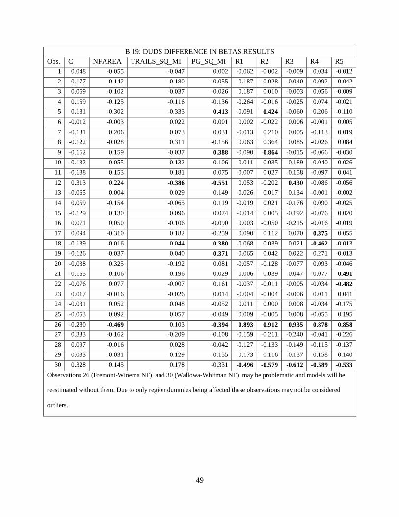
variables (r<0.2).Outliers found in DUDS, OUDS, and GFA models for Difference in Betas

(Tables B15-B18) were removed and new estimates are documented in Appendix B Table B14.

16

TABLE 4: INITIAL DUDS MODEL

Variable Estimate Std Error P-value Elasticity

Constant 7.9558 0.8047 0.0000** N/A

National Forest Area 0.0002 0.0001 0.0416** ∆Sq miles of NF*0.02= %∆ annual vd

Trails per sq mile 3.2078 1.1788 0.0128** ∆trail miles*320= %∆ annual vd

Picnic Grounds per sq mile 98.659 62.372 0.1286 ∆PG/sq mile of NF*9866= %∆ annual vd

Region 1 1.1592 0.7091 0.117 If in Region 1=115% increase in annual vd

Region 2 1.9721 0.9536 0.0512* If in Region 2=197% increase in annual vd

Region 3 2.4715 0.7423 0.0032** If in Region 3=247% increase in annual vd



* Variables are significant at the 10% level. **5% level. With White’s standard errors and weighted.

R-squared 0.4734 Adjusted R-squared 0.2728

S.E. of regression 1.0015 F-statistic 2.3600

Prob(F-statistic) 0.0550 N=30

Listed as (S2ln_d) in Appendix B: Table B6

TABLE 5: INITIAL OUDS MODEL


Constant 6.8504 0.8067 0.0000** N/A

Campgrounds per sq mile 131.206 42.0783 0.0054** ∆CG/ sq mile*13,120= %∆ annual vd

Trails per sq mile 2.1607 1.1544 0.0760** ∆trail miles/ sqmile of NF*216= %∆ annual vd

National Forest Area 0.0003 0.0001 0.0001** ∆Sq miles of NF*0.03= %∆ annual vd

Next to National Park 0.4402 0.2194 0.0585* If Next to NP=44% increase in annual vd

Region 1 -0.0275 0.3518 0.9385 If in Region 1=3% decrease in annual vd



Region 4 -0.0238 0.3612 0.948 If in Region 4=2% decrease in annual vd






Listed as (S2ln_c) in Appendix B: Table B8

17

TABLE 6: INITIAL GFA MODEL


Constant 11.7215 0.8161 0.0000** N/A

Trails per sq mile 2.5368 1.0132 0.0206** ∆trail miles/ sqmile of NF*253= %∆ annual vd

National Forest Area 0.0002 0.0001 0.1021 ∆Sq miles of NF*0.02= %∆ annual vd

Proximity to Nearest

Metropolitan -0.0036 0.0028 0.2112

∆ miles to NF*-0.36= %∆ annual vd










Listed as (S2ln_c) in Appendix B: Table B10

TABLE 7: INITIAL WILDERNESS MODEL


Constant 8.7903 0.3894 0.0000** N/A

Wilderness Trail Miles 0.0015 0.0008 0.0693*

∆wilderness trail miles*0.15= %∆ annual vd

State High Point in

Wilderness

1.2829 0.487 0.0140** If State High Point in Wilderness Area=128%

increase in annual vd

Wilderness Areas w/in 100

miles

0.0129 0.0049 0.0149** # of other Wilderness Areas w/in 100 miles

of NF* 1.3=%∆ increase in annual vd





Listed as (S2ln_d) in Appendix B: Table B11

Hypothesis Testing

Explained variance of visitation was best for OUDS at 55% and lowest for Wilderness at

18%. Low explanatory power with Wilderness may be due to difficulty in measuring a good

proxy for wilderness access (e.g. # of trailheads leading into Wilderness area, or distance to

18

Wilderness area from trailhead. See Table 3). These descriptive candidate models will serve as

predictive models in the next section. The only modifications will be removing outliers and

testing WLS, for the concern of simplicity in reapplication to other National Forests.

H0: USFS annual visitor use by type is not related to bio-physical features of the

landscape, facilities, and distance to population centers.

Ha: Visitor use by type is related to site characteristics.

Reject null hypothesis. For DUDS, the coefficients for NF Area, Trails per sq mile,

Picnic grounds per sq mile, and Regions 2, 3, and 5 are statistically significant. OUDS was

explained by Campgrounds per sq mile, Trails per sq mile, NF Area, Adjacent to National Park,

and Regions 2-3 with statistical significance. GFA model had statistically significant coefficients

for NF area, Regions 2, and 5. Wilderness had statistically significant Wilderness Trails, State

High Point in wilderness, and substitutes.

The shared significant variables between DUDS, OUDS, and GFA models meet a priori

expectations that the different types of NF visitation have similar dependencies. Nation Forest

area (NFArea) is positive and significant at the 10% level in for OUDS, DUDS, and GFA.

Region Two (Colorado and Wyoming) is positive and significant in those three models as well.

Trails per square mile is significant at the 5% level in DUDS and OUDS, but is at the 20%

confidence level for GFA. This is helpful for application of models on BLM lands. Wilderness

models do not share common variables with the other three recreation types besides proxies for

travel cost.

19

2. OUT OF SAMPLE ESTIMATION

2.1 Prediction Models

Candidate models for the four recreation types were used to estimate out of sample

visitation. Multiple predictions were conducted for each candidate model due to alternative

forms from weighting and outlier diagnostics. Appendix B shows the natural log of actual

visitation, predicted values from each alternative model, and prediction accuracy. This study

will use Mean Absolute Percentage Error (MAPE) to compare predictive power of each model

(Tables B19-B22).

TABLE 8: PERFORMANCE OF INITIAL CANDIDATE MODELS

See Tables B 23- B 26 MAPE

DUDS 103% - 207%

OUDS 93% - 105

GFA 115% - 152%

Wilderness 68% - 76%

See Appendix B: Tables B:23-B26 for equations

The interpretation of MAPE for DUDS is that on average, the absolute value of the

difference between the predicted values and the actuals was lowest at 103%. MAPE does not

capture if the errors are bias upward or downward and a different metric could reveal which is

the case. Due to all of the predicted values being positive, it can be concluded that the

predictions are biased to overestimate. If the models were typically underestimating and had a

MAPE of more than 100%, negative predictions would have to be present. The range in MAPE

for each recreation type comes from different predicted values of multiple versions of the initial

20

models. The different versions of the model were with and without potential outliers, weighted

and unweighted, and with different log transformation bias correctors (See Appendix B: Tables

B23-26)

Alternative Prediction opportunities

It is uncertain if the inaccuracy with out of sample prediction came from the lack of a

representative sample or weak explanatory power of the independent variables. Comparing

representativeness sub-samples can be found by using a program to comprehensively estimate

and rank the explanatory power of all combinations that leave out 25% of the observations. This

process would reveal a representative sample and the distribution of model explanatory power.

Conclusions about representative sites would benefit the BLM and USFS with which sites will

have more accurate predictions and which ones would require additional on-site sampling.

Unfortunately, such a complex and time intense modeling effort is beyond the scope of this

thesis. The stratified sampling in NVUM of low, medium, high, very high, and closed for

visitation could be used when transferring this model from USFS lands to BLM lands. There is a

class of literature on estimates using a stratified sample that could help if BLM visitation was

assumed to be a level below USFS visitation. This method requires a much more intricate

econometric model with heavy assumptions about the relationship between USFS and BLM

visitation.

2.2 Stepwise Procedures

Using all 40 observations in a stepwise procedure is another approach to finding the

explanatory power of the independent variables. For each recreation type there was a stepwise

estimation using a full specification of their unique independent variables (see Appendix C). A

21

combinatorial procedure revealed which independent variable contributes the most to explaining

visitation. Appendix C outlines the best models using one to five regressors, or until models had

econometric issues. Collinearity became an issue in the combinatorial procedure when using

more than five regressors due highly correlated variables in the pool of regressors to choose

from. To deal with this, combinatorial results from one to three regressors were tested for

improvements from additional uncorrelated variables. Candidate models were constructed by

this method.

TABLE 9: STEPWISE DUDS MODEL


Constant 11.63 0.3528 0.0000** N/A

Miles of Rivers 0.000043 0.0000 0.0349** ∆river miles in NF*0.0043= %∆ annual vd

Picnic Grounds 0.03 0.0102 0.0175** ∆# of PG in NF*3= %∆ annual vd

R1 0.37 0.3791 0.3380 If in Region 1=37% increase in annual vd

R2 0.89 0.3398 0.0130** If in Region 2=89% increase in annual vd




* Variables are significant at the 10% level. **5% level.




22

TABLE 10: STEPWISE OUDS MODEL


Constant 9.6502 0.3581 0.0000** N/A

Campsites 0.0012 0.0003 0.0002** ∆# of CS in NF*0.12= %∆ annual vd

Area of National Forest 0.0001 0.0001 0.0878* ∆Sq miles of NF*0.01= %∆ annual vd

R1 -0.3643 0.4358 0.4094 If in Region 1=36% decrease in annual vd





* Variables are significant at the 10% level. **5% level




TABLE 11: STEPWISE GFA MODEL


Constant 11.5091 0.5213 0.0000** N/A

Miles of Rivers 0.0001 0.0000 0.0158** ∆river miles in NF*0.01= %∆ annual vd

Trails per sq mile 1.0777 1.0324 0.3043 ∆trail miles/ sqmile of NF*107= %∆ annual vd


R2 0.8433 0.4886 0.0940* If in Region 2=84% increase in annual vd




* Variables are significant at the 10% level. **5% level. With White’s standard errors.




23

TABLE 12: STEPWISE WILDERNESS MODEL


Constant 7.6519 0.4605 0.0000** N/A

Miles of Wilderness

Trails 0.0012 0.0007 0.0866*

∆wilderness trail miles in NF*0.12= %∆ annual

vd

Number of Wilderness

Areas in the National

Forest

0.1276 0.0477 0.0118** # of other Wilderness Areas in NF* 13=%∆


State High Point in

Wilderness Area 0.6766 0.5364 0.2165

If State High Point in Wilderness Area=68%







* Variables are significant at the 10% level. **5% level. With White’s standard errors.




3. SPREADSHEET CALCULATOR

A National Forest and BLM land visitation calculator that uses the stepwise models

(Tables 14-17) is available upon request. Uses of the calculator vary from estimating visitation

on a yet to be sampled land, double checking recently estimated visitation, or conducting

marginal analyses on changes in visitation from a change in facilities.

4. DISCUSSION AND CONCLUSION

Elasticity of visitation with respect to site characteristics is calculated by multiplying beta

estimates in the semi-log models by 100. For example, the elasticity of day use developed

visitation with respect to picnic grounds in the stepwise models is 3, meaning a new additional

Picnic ground will increase annual visitation by 3%. Very interesting is the difference in regional

elasticities across the different recreation types. Furthermore, the difference in regional

elasticities between the initial models and the stepwise is significant. Interpretation of

24

modifiable characteristics such as campground, trail, and other facility elasticities are relevant to

planners and managers. The spreadsheet calculator can help quantify visitation change from a

new campground by looking at the difference in estimates with the current number of

campgrounds and the proposed new ones. Effects on annual visitation from land sales or

purchases can be estimated. Supplemental information beneficial to planners may be differences

in elasticities between regions and USFS or BLM sites that may predict better than others.

Explanatory power of the initial models (n=30) and stepwise models (n=40) were similar

for some recreation types, with two out of four improving. DUDS models did not change much

between the sample sizes, with the initial model having an adjusted R2 of 0.27 and stepwise

improving to 0.29. OUDS also saw little change, changing from 0.55 to 0.46. GFA lowered from

0.28 to 0.19. Wilderness saw a substantial improvement between the two sample sizes, going

from 0.18 to 0.47. Those than improved gained from estimating with a full sample, while those

that worsen had ambiguous information gains.

The weak to moderate explanatory and predictive power in these models should give

some caution in the applicability of this type of visitor use estimation. The statistically

significant site characteristics provide optimism in continued development of this method. A

recommended next step in this research would be revisiting variable selection or getting more out

of the current dataset with the above mentioned testing of all out of sample combinations.

Removing the uncertainty in the change in significant variables between 30 and 40 observations

may or may not be worth the effort. Time series analysis is not feasible with NVUM data until

2015 but would provide valuable insight to changes in facility elasticities and visitation over

time. Nonetheless, these models provide a cost effective, objective and systematic approach to

estimating visitation on BLM lands until on-site sampling can be conducted on all BLM lands.

25

These models also provide estimates of the statistical accuracy of the visitation predictions as

well as upper and lower ranges in visitation that can be used for sensitivity analysis.

Assigning sampling points of interest similar to NVUM on non-sampled BLM lands

could be another transfer method. This method could be especially bountiful for BLM lands that

share borders with sampled NF’s. The study shows the mathematical and data requirements to

estimate visitor use in watershed within a national forest and if that watershed was spread across

two national forests. Estimating visitation for an entire forest is much easier than estimating a

sub region, especially if NVUM did not sample within that sub region. (White et al 2007) The

model is also capable of estimating visitation in a “new forest” where NVUM sampling has not

occurred.

Other research ideas for visitor use estimation methods are incorporating choice

experiments on recreation factors with NVUM data. Fredman and Lindberg (2006) combined

stated preferences on facilities and other site characteristics with visitor counts at multiple cross

country skiing sites in Sweden. This method allows for better variable creation and improved

explanation of the variance. To apply this on NF or BLM lands would be feasible and would

improve the understanding of what drives recreation at a finer scale than this project. Substitute

data for this method could come from existing hotspot studies in the United States.

26

REFERNCES

Bowker, J. M., Askew, A., Seymor, L., Zhu, J.P., English, D.B.K., & Starbuck, C.M. (2009).

Wilderness Recreation Demand: A Comparison of Travel-Cost and On-site Models. In:

Zinkhan, C. & Stansell, B.(eds.) Southern Forest Workers: proceedings of the annual

meeting; 2009. Chapel Hill, NC: The Forestland Group. 156-164

Bowker, J. M, Murphy, D., Cordell, H.K., English, D.B.K., Bergstrom, J.C., Starbuck, C. M.,

Betz, C. J., Green, G.T., & Reed. P. (2007). Wilderness Recreation Participation:

Projections for the Next Half Century. USDA Forest Service Proceedings RMRS-P-49.

Bowker, J.M., Murphy, D., Cordell, H.K., English, D.B.K., Bergstrom, J.C., Starbuck, C.M.,

Betz, C.J., & Green, G.T. (2006). Wilderness and Primitive Area Recreation Participation

and Consumption: An Examination of Demographic and Spatial Factors. Journal of

Agricultural and Applied Economics. 32,2. p 317-326.

Bowker, J.M., English, D.B.K., Bergstrom, J.C., & Starbuck, C.M. (2005). Valuing National

Forest Recreation Access: Using a Stratified On-Site Sample to Generate Values across

Activities for a Nationally Pooled Sample. Selected Paper from 2005 AAEA Meetings.

Providence, Rhode Island: July 24-27.

Brown, G. (2008). A Theory of Urban Park Geography. Journal of Leisure Research. 40, 4. 589-

607.

Brown, G. & Alessa, L. (2005). A GIS-based Inductive Study of Wilderness Values.

International Journal Of Wilderness. 11, 1.

27

Cole, D. N. (1996). Wilderness Recreation Use Trends, 1965 through 1994. United States

Department of Agriculture, Forest Service Intermountain Research Station. Ogden, UT.

INT-RP-488

Cordell, H.K., Tarrant, M. A., McDonald, B. L., & Bergstrom, J. C. (1998). How the Public

Views Wilderness: more results from the USA survey on recreation the environment.

International Journal of Wilderness. 4,28-31.

Cordell, H.K., Tarrant, M. A., Green, G.T. (2003). Is the Public Viewpoint of Wilderness

Shifting? International Journal of Wilderness. 9, 2.

De Vries, S. & De Boer, T.A. (2006). Recreational Accessibility of Rural Areas: Its Assessment

and Impact on Visitation and Attachment. Presented at Planning and managing forests for

recreation and tourism. Wageningen: May 30.

De Vries, S., Lankhorst, J. R. & Buijs, A. E. (2007). Mapping the attractiveness of the Dutch

countryside: a GIS-based landscape appreciation model. Forest, Snow and Landscape

Research. 81,43-58.

Dumont, B. & Gulinck, H. (2004). Push and pull assemblages for modeling visitor’s flows in

complex landscapes. Working Papers of the Finnish Forest Research Institute 2.

Retrieved (January 2012) from www.metla.fi/julkaisut/workingpapers/2004/mwp002-

57.pdf

English, D.B.K., Kocis, S.M., Zarnoch, S.J., & Arnold, J.R. (2002). Forest Service National

Visitor Use Monitoring Process: Research Method Documentation. USFS Southern

Research Station. Asheville, North Carolina. Research Paper SRS-57.

28

English, D.B.K. (unknown). National Visitor Use Monitoring (NVUM). Presentation at Colorado

State Univeristy.

Fredman, P. & Lindberg, K. (2006). Swedish Mountain Tourism Patterns and Modelling

Destination Attributes. In: Gossling, S. & Hultman, J. (eds.) Ecotourism in Scandanavia:

Lessons in Theory and Practice. CAB International.

Loomis, J. (1999). Do Additional Designations of Wilderness Result in Increases in Recreation

Use? Society & Natural Resources: An International Journal. 12,5. P 481-491.

Loomis, J. (2000). Counting on Recreation Use Data: A Call for Long-Term Monitoring. Journal

of Leisure Research.32, 1. P 93-96.

Loomis, J. (2000). Economic Values of Wilderness Recreation and Passive Use: What We Think

We Know at the Beginning of the 21st Century. USDA Forest Service Proceedings.

RMRS-P: 15,2.

Loomis, J. & Richardson, R. (2000). Economic Values of Protecting Roadless Areas in the

United States. Prepared for The Wilderness Society and Heritage Forests Campaign.

Accessed October 2011 from

http://wilderness.org/files/Economic%20Values%20of%20Protecting%20Roadless%20A

reas%20in%20US.pdf

Manning, R.E., Newman, P., Fristrup, K. Stack, D.W., & Pilcher, E. (2010). A program of

research to support soundscape management at Muir Woods National Monument. Park

Science. 26,3. P 54-57.

29

Newman, P., Manning, R., & Dennis, D. (2005). Informing Social Carrying Capacity Decision

Making in Yosemite National Park, Using Stated Choice Modeling. Journal of Parks and

Recreation Administration. 21,3. P 43-56.

Newman, P., Marion, J, & Cahill, K. (2001). Integrating resource, social, and managerial

indicators of quality into carrying capacity decision making. The George Wright Forum.

18,3. P 28-40.

Stack, D.W., Newman, P., & Manning, R. (2011). Protecting Soundscapes in our National Parks:

An Adaptive Management Approach in Muir Woods National Monument. Journal of the

Acoustic Society of America. 129,3. P 1375-1380.

Stynes, D.J., Peterson, G. L., & Rosenthal, D. H. (1986). Log Transformation Bias in Estimating

Travel Cost Models. Land Economics. 62,1. P 94-103.

United States Department of the Interior, Bureau of Land Management. (2003). The BLM’s

Priorities for Recreation and Visitor Services: BLM Workplan, Fiscal Year 2003-2007

(BLM Purple book). Washington, D.C.

United States Department of the Interior, Bureau of Land Management. (2005). BLM Land Use

Planning Handbook. H-1601-1. Washington, D.C.

United States Department of the Interior, Bureau of Land Management . (2010). Annual

Performance Report: FY 2010. Washington, D.C.

30

United States Department of the Interior, Bureau of Land Management . (2011). Budget

Justifications and Performance Information Fiscal Year 2012. Washington, D.C.

United States Department of Agriculture, Forest Service. (2010). National Visitor Use

Monitoring Results: National Summary Report. Accessed October 2011 from

http://www.fs.fed.us/recreation/programs/nvum/nvum_national_summary_fy2009.pdf

United States Department of Agriculture, Forest Service. (2007). National Visitor Use

Monitoring Results for Moab Field Office. National Visitor Use Monitoring Program.

Moab, UT.

United States Department of Agriculture, Forest Service (2006). National Visitor Use

Monitoring Definitions. Accessed October 2011 from

http://www.fs.fed.us/recreation/programs/nvum/reference/prework_definitions.pdf

Wang, J. (2008). Development of Outdoor Recreation Resource Amenity Indices for West

Virginia. (Master’s Thesis). West Virginia University. Morgantown, West Virginia.

Watson, A.E., Cole, D.N., Turner, D.L., & Reynolds, P.S. (2000). Wilderness Recreation Use

Estimation: A Handbook of Methods and Systems. Rocky Mountain Research Station.

Ogden, UT. RMRS-GTR-56.

White, E. M., Zarnoch, S. J., & English, D.B.K. (2007). Area-Specific Recreation Use

Estimation Using the National Visitor Use Monitoring Program Data. USFS Pacific

Northwest Research Station. Corvallis, Oregon. Research Note PNW-RN-557.

Wooldridge, J. M. (2000). Introductory Econometrics: A Modern Approach. Cincinnati: South-

Western College Pub.

31

Zarnoch, S.J., English, D.B.K., & Kocis, S. M. (2005). An Outdoor Recreation Use Model With

Applications to Evaluating Survey Estimators. United States Forest Service, Southern

Research Station. Athens, Georgia. Research Paper SRS-37.

Ziemer, R.F., Musser, W. N., & Hill, R.C. (1980). Recreation Demand Equations: Functional

Form and Consumer Surplus. American Journal of Agricultural Economics. 62, 1. P 136-

141.

32

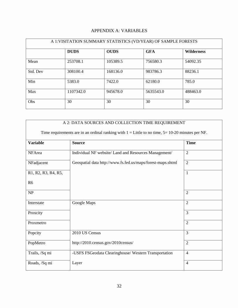
APPENDIX A: VARIABLES

A 1:VISITATION SUMMARY STATISTICS (VD/YEAR) OF SAMPLE FORESTS

DUDS OUDS GFA Wilderness

Mean 253708.1 105389.5 756580.3 54092.35

Std. Dev 308100.4 168136.0 983786.3 88236.1

Min 5383.0 7422.0 62180.0 785.0

Max 1107342.0 945678.0 5635543.0 488463.0

Obs 30 30 30 30

A 2: DATA SOURCES AND COLLECTION TIME REQUIREMENT

Time requirements are in an ordinal ranking with 1 = Little to no time, 5= 10-20 minutes per NF.

Variable Source Time

NFArea Individual NF website/ Land and Resources Management/

Geospatial data http://www.fs.fed.us/maps/forest-maps.shtml

2

NFadjacent 2

R1, R2, R3, R4, R5,

R6

1

NP 2

Interstate Google Maps 2

Proxcity 3

Proxmetro 2

Popcity 2010 US Census

http://2010.census.gov/2010census/

3

PopMetro 2

Trails, /Sq mi -USFS FSGeodata Clearinghouse/ Western Transportation

Layer

4

Roads, /Sq mi 4

33

WildTrails, /Sq mi http://fsgeodata.fs.fed.us/vector/index.html

-Individual NF website/ Land and Resources Management/


3

Lakes, /Sq mi 3

LakeArea, /Sq mi 3

Rivers, /Sq mi 3

WildLakes, /Sq mi 3

WildLakeArea, /Sq mi 3

WildRivers, /Sq mi 4

PG, /Sq mi Individual NF website/ Land and Resources Management/


Individual NF SBS Maps:

http://fsgeodata.fs.fed.us/visitormaps/

Paper Maps for each NF were also used for CG count

5

PGElev 5

CG, /Sq mi 5

CGLake 5

CS, /Sq mi 5

CGElev 5

HighPointElev Individual NF Maps,

Peakbagger List of state High Points

http://www.peakbagger.com/list.aspx?lid=1825

3

StateHigh 2

WildHighPoint 3

WildStateHigh 2

WildArea Wilderness Boundaries GIS Layer

http://nationalatlas.gov/mld/wildrnp.html

2

Wilderness Dummy 2

Wilderness count 2

Wilderness w/in 100

mi

2

More Links:

Region GIS Database:

R1: http://www.fs.fed.us/r1/gis/ThematicTables.htm

34

R2: http://www.fs.fed.us/r2/gis/datasets_unit.shtml

R4: http://www.fs.fed.us/r4/maps/gis/index.shtml

R5: http://www.fs.fed.us/r5/rsl/clearinghouse/VisitorMaps.shtml

R6: http://www.fs.fed.us/r6/data-library/gis/index.html

NVUM Annual Visitation Page http://apps.fs.usda.gov/nrm/nvum/results/

Special thanks to Mike Hadley, USFS Geospatial services and Technology Center, UT for help with Maps

35

APPENDIX B: CANDIDATE MODELS

B 1: DUDS FULL

SPECIFICATIONS

Specification

1 (S1)

Specification

2 (S2)

NF Area NF Area

PG/ Sq mi PG/ Sq mi

PG Elev PG Elev

Pop Metro Pop Metro

Prox Metro Prox Metro

Interstate R1-R5

State High

Point

High Point

Trails Interstate

Lake Area Lake Area

River/ Sq mi River/ sq mi

B 2: OUDS FULL

SPECIFICATIONS

Specification 1

(S1)

Specification 2

(S2)

CG CG/ sq mi

CG Elev CS/ sq mi

CS Interstate

Interstate River/ Sq mi

Trails Trails/ sq mi

NF Area NF Area

NP Adjacent NP Adjacent

Pop Metro Pop Metro

R1-R5 R1-R5

B 3:GFA FULL SPECIFICATIONS

Specification 1

(S1)

Specification 2

(S2)

High Point State High Point

Interstate Interstate

Lake Area Lake Area

River/ sq mi River/ sq mi

Road/ sq mi Road/ sq mi

Trail/ sq mi Trail/ sq mi

NF Area NF Area

Pop Metro Pop Metro

R1-R5 Trails

B 4: WILDERNESS UNIQUE VARIABLES

Variable Description Measurement

WildArea Area of Wilderness Area(s) Sq. Miles

WildTrails, / sq mile Total Length of Wilderness Trails Miles, miles/sq mi

WildHighPoint NF high point within Wilderness Boundary Dummy Variable

WildStateHigh NF high point is State high point and within Wilderness

Boundary Dummy Variable

WildLakes, / sq mile Number of water bodies in Wilderness Boundary # count, n/sq mile

WildLakeArea, / sq

mile Total Area of water bodies in Wilderness Boundary Sq. Miles

WildRivers, / sq mile Sum of River Lengths in Wilderness Boundary Miles, miles/sq mile

WildArea/sqmi Sq mile of Wilderness Area per sq mile of NF Sq mile/ sq mile

Wilderness Dummy =1 if there is more than one wilderness in NF, =0 if there is

only one wilderness area within NF Dummy Variable

Wilderness count # of wilderness areas adjacent to NF. Includes NPS, BLM,

FWS wilderness areas # count

36

Wilderness substitutes

w/in 100 mi

# of wilderness areas within 100 miles of NF. Includes NPS,

BLM, FWS wilderness areas # count

B 5: LINEAR DUDS MODELS S1_a S1_b S1_c S2_a S2_c

HighPointElev (0.1927) (0.0538)* (0.0162)** (0.0783)* (0.0275)**

Nfarea (0.4390) (0.9041) (0.9029) (0.6977) (0.6899)

Np

Pg

Pg_sq_mi (0.0717)* (0.0655)* (0.0583)* (0.0510)* (0.0437)**

Pgelev (0.5656) (0.8173) (0.8226)

Popmetro (0.3718) (0.3579)

Proxmetro

R1 (0.5704)

R2 (0.7648)

R3 (0.1928) (0.0651)* (0.0426)** (0.0471)* (0.0300)**

R4 (0.5239)

R5 (0.2426)

River_sq_mi (0.5353)

Trails_sq_mi (0.3484) (0.7332) (0.7127)

k=12 k=7 k=5 k=8 k=6

adjR2=0.1221 adjR

2=0.1776 adjR

2=0.2376 adjR

2=0.1715 adjR

2=0.2339

Se(Y)=300872.6 Se(Y)=291195.2 Se(Y)=280370 Se(Y)=292270 Se(Y)=281052

F=1.366 F=2.044 F=3.26 F=1.85 F=2.77

P=(0.2686) P=(0.1004) P=(0.0278) P=0.1260 P=0.0410


37

B 6: LOG-LINEAR DUDS MODELS

S1ln_c S1ln_d S2Ln S2LN_d

(Candidate)

S2LN_b

HighPointElev

Interstate (0.4483)

Lakearea (0.1594) (0.0636)*

Nfarea (0.2229) (0.1653) (0.8634) (0.1653) (0.0449)**

Pg_sq_mi (0.1254) (0.1249) (0.0750)* (0.1249) (0.0363)**

Pgelev (0.2707)

Popmetro (0.5337)

Proxmetro (0.7373) (0.7001)

R1 (0.1611) (0.1413) (0.) (0.1422)

R2 (0.0159)** (0.0134)** (0.1596) (0.0267)**

R3 (0.0031)** (0.0014)** (0.0442)** (0.0067)**

R4 (0.2974) (0.3042) (0.9413) (0.6994)

R5 (0.0077)** (0.0053)** (0.0020)** (0.0017)**

River_sq_mi (0.5548)

Rivers

Statehp (0.7491)

Trails (0.7586)

Trails_sq_mi (0.0891)* (0.0873)* (0.9304) (0.0873)* (0.0561)*

k=10 k=9 k=12 k=9 k=10

adjR2=0.2451 adjR

2=0.2769 adjR

2=-0.0959 adjR

2=0.2769 adjR

2=0.3635

Se(Y)=1.1473 Se(Y)=1.1229 Se(Y)=1.3825 Se(Y)=1.1229 Se(Y)=1.05

F=2.04 F=2.388 F=0.769 F=2.388 F=2.840

P=(0.08746) P=(0.0525) P=(0.6653) P=(0.00525) P=(0.0248)


38

B 7:OUDS LEVEL EXPLANATORY VARIABLES

S1 S1_a S1_b S1_Ln S1_Ln_a S1_Ln_b

CG (0.6694) (0.5421) (0.5791)

CG

Elevation

(0.6243) (0.5694) (0.2728) (0.2176) (0.2623)

Campsites (0.0292)** (0.0051)** (0.000)** (0.6832) (0.0038)** (0.0010)**

Interstate (0.7061) (0.0999)** (0.4671)

NF Area (0.9357) (0.9670)

NP (0.8744) (0.2693) (0.1948) (0.3343)

PopMetro (0.9091) (0.9797)

ProxMetro (0.4232) (0.2311) (0.2306) (0.5949) (0.3719)

R1 (0.8581) (0.8566) (0.9596) (0.7390) (0.5466) (0.3692)

R2 (0.6641) (0.5540) (0.2536) (0.3947) (0.2862) (0.4514)

R3 (0.0586)* (0.0234)** (0.0219)** (0.0363)** (0.0232)** (0.0173)**

R4 (0.9347) (0.9535) (0.7924) (0.7788) (0.8728) (0.8967)

R5 (0.5367) (0.3275) (0.3442) (0.8072) (0. 8246) (0.6832)

Trails (0.8818) (0.4087) (0.0891)* (0.0897)*

k=15 k=10 k=8 k=15 k=8 k=9

adjR2=0.408 adjR

2=0.5485 adjR

2=0.5728 adjR

2=0.4743 adjR

2=0.5501 adjR

2=0.5700

Se(Y)=84685.6 Se(Y)=73969.4 Se(Y)=71947.2 Se(Y)=0.6808 Se(Y)=0.6298 Se(Y)=0.6157

F=2.429 F=4.915 F=6.55 F=2.86 F=4.22 F=5.27

P=(0.049630) P=(0.00147) P=(0.00029) P=(0.0259) P=(0.000345) P=(0.000962)


39

B 8: OUDS DENSITY EXPLANATORY VARIABLES

S2

(Full

Specification)

S2_a S2_b

S2Ln

(Full

Specification)

S2Ln_b S2Ln_c

(Candidate)

CG/sqmi

forest

(0.2626) (0.2566) (0.3100) (0.1802) (0.0031)** (0.0052)**

CS/sqmi

of forest

(0.1660) (0.0736)* (0.0347)** (0.4644)

Interstate (0.9601) (0.8198)

Mi Trails/

sqmi of

forest

(0.3750) (0.2001) (0.1303) (0.0815)* (0.0442)** (0.0325)**

NF Area (0.0277)** (0.0110)** (0.0055)** (0.0087)** (0.0006)** (0.0027)**

NP (0.8769) (0.2068) (0.0825)* (0.0580)*

PopMetro (0.8618) (0.8639)

ProxMetro (0.6321) (0.5466) (0.3758)

R1 (0.6999) (0.7694) (0.9130) (0.9265) (0.0605)*

R2 (0.9178) (0.7588) (0.2953) (0.0896)* (0.0024)**

R3 (0.0446)** (0.0320)** (0.0219)** (0.0329)** (0.0011)** (0.9909)

R4 (0.7631) (0.7909) (0.7707) (0.8933) (0.7377)

R5 (0.5992) (0.5227) (0.9790) (0. 7694) (0.8910)

k=14 k=10 k=6 k=14 k=10 k=11

adjR2=0.3310 adjR

2=0.4430 adjR

2=0.503 adjR

2=0.4769 adjR

2=0.5425 adjR

2=0.5384

Se(Y)=90039.8 Se(Y)=82157.6 Se(Y)=77599.6 Se(Y)=0.6791 Se(Y)=0.6351 Se(Y)=0.6379

F=2.10 F=3.563 F=6.87 F=3.034 F=4.822 F=4.38

P=(0.0800) P=(0.008594) P=(0.000414) P=(0.01910) P=(0.0016) P=(0.0027)


40

B 9: GFA LEVEL EXPLANATORY VARIABLES

S1_a

(Full

Specification)

S1_b S1_c S1_Ln_a S1_Ln_b S1_Ln_c

NFarea (0.3763) (0.4185) (0.5262) (0.4491) (0.7427)

Interstate (0.5813)

Roads (0.3321)

PopMetro (0.2565) (0.2966) (0.1171)

ProxMetro (0.0388)** (0.0229)** (0.0077)** (0.4225) (0.3196) (0.1826)

Lake Area (0.7332) (0.8550)

State High

Point

(0.3781) (0.4382) (0.3750)

Trails (0.2727) (0.2727) (0.2094) (0.2686) (0.2427)

R1 (0.5971) (0.5348) (0.5358) (0.4492) (0.1183)

R2 (0.1131) (0.0659)* (0.0151)** (0.1651) (0.0251)** (0.0074)**

R3 (0.7094) (0.07994) (0.8580) (0.8892) (0.8322)

R4 (0.6849) (0.7363) (0.9225) (0.8207) (0.6511)

R5 (0.9162) (0.7623) (0.1957) (0. 0542)* (0.0426)**

k=12 k=11 k=7 k=11 k=10 k=8

adjR2=0.322 adjR

2=0.3466 adjR

2=0.4121 adjR

2=0.1499 adjR

2=0.1503 adjR

2=0.222

Se(Y)=839256 Se(Y)=823996 Se(Y)=781633 Se(Y)=0.90185 Se(Y)=0.901 Se(Y)=0.8623

F=2.25 F=2.538 F=4.388 F=1.511 F=1.57 F=2.188

P=(0.0608) P=(0.0386) P=(0.00426) P=(0.2102) P=(0.1914) P=(0.0759)


41

B 10: GFA DENSITY EXPLANATORY VARIABLES

S2_a S2_c S2_d S2Ln_a S2Ln_b

S2Ln_c

(Candidate)

NF Area (0.1999) (0.0576)* (0.0493)** (0.3162) (0.2901) (0.1455)

Interstate (0.6950) (0.6557)

River/ sqmi (0.2347) (0.5822) (0.5888)

Lake Area (0.8819) (0.8727) (0.7999)

Road/ sqmi

forest

(0.6696) (0.4232) (0.3570)

Trails/ sqmi

forest (0.0985)* (0.1285) (0.1353) (0.0975)* (0.0869)* (0.0650)*

PopMetro (0.6625) (0.3002) (0.1216)

ProxMetro (0.0240)** (0.0175)** (0.0056)* (0.2100) (0.2183) (0.2232)

State High

Point

(0.5832) (0.2704) (0.2431)

R1 (0.9912) (0.4639) (0.4983) (0.5666) (0.3135)

R2 (0.0790)* (0.0538)* (0.0130)** (0.0697)* (0.0701)* (0.0079)**

R3 (0.5600) (0.8754) (0.7927) (0.8714) (0.6959)

R4 (0.4670) (0.5959) (0.8942) (0.8568) (0.8640)

R5 (0.5549) (0.6523) (0.1173) (0. 1221) (0.0249)**

k=15 k=11 k=7 k=13 k=12 k=9

adjR2=0.3095 adjR

2=0.3845 adjR

2=0.4289 adjR

2=0.1551 adjR

2=0.1924 adjR

2=0.2648

Se(Y)=847056 Se(Y)=799726 Se(Y)=770347 Se(Y)=0.8991 Se(Y)=0.8790 Se(Y)=0.8387

F=1.92 F=2.812 F=4.63 F=1.44 F=1.628 F=2.305

P=(0.1096) P=(0.0251) P=(0.00318) P=(0.2378) P=(0.1730) P=(0.0598)


42

B 11: WILDERNESS LEVEL EXPLANATORY VARIABLES

S1ln S1ln_a S2ln S2Ln_b S2Ln_c S2Ln_d

(Candidate)

Wild Area (0.3904) (0.2377)

Pop City (0.8156)

Prox City (0.4692)

WState High (0.4043) (0.3930) (0.1748) (0.0549)*

R1 (0.5082) (0.6610)

R2 (0.5281) (0.3488) (0.3180)

R3 (0.5089) (0.3773) (0.5974)

R4 (0.9132)

R5 (0.9280) (0.8387) (0.7382)

R6 (0.3732) (0.3580) (0.5044)

Wild Trail (0.0454)** (0.0682)*

Pop Metro (0.6878)

Wild HP (0.6922)

WLake Area (0.3209)

Wild Subs (0.1756)

k=10 k=8 k=11 k=4

adjR2=0.089 adjR

2=0.149 adjR

2=0.1810 adjR

2=0.1938

Se(Y)=1.38 Se(Y)=1.335 Se(Y)=1.309 Se(Y)=1.299

F=1.316 F=1.72 F=1.64 F=3.324

P=(0.2892) P=(0.1545) P=(0.1693) P=(0.0351)


43

B 12: WILDERNESS DENSITY EXPLANATORY VARIABLES

S3ln S3ln_a S4 S4Ln_a S4Ln_b S4Ln_c

Wild Area (0.1522) (0.1559)

WTrail/sq mi (0.3508) (0.5023)

Wild Trail (0.2934) (0.1927) (0.1932) (0.1883)

WLkArea/sq

mi

(0.2190) (0.8623) (0.1285) (0.2093) (0.3792)

WRiver/sq mi (0.3743) (0.5556) (0.9477) (0.3598) (0.2242) (0.3742)

Prox Metro (0.5979) (0.7745) (0.5449) (0.7541) (0.6190) (0.8894)

R1 (0.7270) (0.9652)

R2 (0.5076) (0.3991) (0.6859) (0.4134) (0.5860)

R3 (0.7516) (0.5237) (0.3486) (0.7185) (0.8818)

R4 (0.8580) (0.9655) (0.7350)

R5 (0.7551) (0.8592) (0.7646) (0.9380) (0.8650)

R6 (0.2758) (0.3312) (0.7675) (0.1855) (0.2005)

Wild Subs (0.3356)

k=11 k=10 k=10 k=10 k=5 k=11

adjR2=0.102 adjR

2=0.0751 adjR

2=0.00 adjR

2=0.1441 adjR

2=0.0869 adjR

2=0.1431

Se(Y)=1.37 Se(Y)=1.39 Se(Y)=100000 Se(Y)=1.339 Se(Y)=1.38 Se(Y)=1.33

F=1.33 F=1.26 F=0.56 F=1.54 F=1.69 F=1.48

P=(0.2828) P=(0.3154) P=(0.8080) P=(0.2003) P=(0.1837) P=(0.2200)


44

B 13: DUDS HETEROSKEDASTICITY TESTS

For S2ln_d:

BPG test:

Heteroskedasticity

Not present

Whites test: N/A

Park Test:

Heteroskedasticity

Not Present

Coefficient Estimate SE p-value White’s

SE

White’s P-

Value

NF Area 0.00021 37.91 (0.1653) 0.0001 (0.0502)*

Trail/ sqmi 3.1818 1.02 (0.0873)* 1.1825 (0.0137)**

PG/ Sq mi 104.2363 0.00008 (0.1249) 61.55 (0.1052)

R1 1.819 0.249 (0.1413) 0.7247 (0.1178)

R2 2.0265 0.436 (0.0134)** 0.9557 (0.0461)**

R3 2.5007 0.424 (0.0014)** 0.7599 (0.0035)**

R4 0.9536 0.402 (0.3042) 0.9418 (0.3228)

R5 2.2781 0.531 (0.0053)** 0.8166 (0.0110)**

White's robust standard errors are shown to note any changes. Two Variables

improved to the 5% confidence level. Will use White’s correction.

B 14: OUDS HETEROSKEDASTICITY TESTS

For S2ln_b:

BPG test:

Heteroskedasticity

Not present (0.0673)

Whites test: N/A

Park Test:

Heteroskedasticity

Not Present (0.0868)


SE

White’s P-

Value

CG/ sqmi 127.70 37.91 (0.0031)** 43.89 (0.0087)**

Trail/ sqmi 2.1934 1.02 (0.0442)** 1.169 (0.0753)*

NF Area 0.000342 0.00008 (0.0006)** 0.00006 (0.0000)**

NP 0.4557 0.249 (0.0825)* 0.220 (0.0522)*

R1 -0.0407 0.436 (0.9265) 0.343 (0.9067)

R2 0.7574 0.424 (0.0896)* 0.362 (0.0495)**

R3 1.535 0.402 (0.0011)** 0.554 (0.0119)

R4 -0.068 0.531 (0.8993) 0.369 (0.8556)

R5 0.1461 0.491 (0.7694) 0.549 (0.7930)

White's robust standard errors are shown to note any changes. P values from tests are

close to rejection and these tests are general, so it may be wise to consider robust

standard errors. White’s correction changes significance out of 5% confidence for two

variables.

45

B 15: GFA HETEROSKEDASTICITY TESTS

For S2ln_c:

BPG test:

Heteroskedasticity

present

Whites test: Not

Present

Park Test:

Heteroskedasticity

Present


SE

White’s P-Value

Trails/ Sqmi 2.633 1.352151 (0.0650)* 1.054061 (0.0209)**

NF Area 0.00016 0.000112 (0.1455) 0.000101 (0.1070)

ProxMetro -0.003 0.002857 (0.2232) 0.002896 (0.2293)

R1 0.585 0.566827 (0.3135) 0.406337 (0.1644)

R2 1.704 0.580950 (0.0079)** 0.512015 (0.0032)**

R3 0.209 0.529439 (0.6959) 0.590673 (0.7259)

R4 0.118 0.682253 (0.8640) 0.620011 (0.8505)

R5 1.333 0.551804 (0.0249)** 0.476334 (0.0107)**

White’s robust standard errors improved one variable from 10% to 5% significance level.

Two out of three tests fail to reject presence of heteroskedasticty. Will use White’s

correction.

B 16: WILDERNESS HETEROSKEDASTICITY TESTS

For S4:

BPG test: Not

present

Whites test:

Not Present

Park Test:

Not present

Coefficient Estimate SE p-value White’s SE White’s P-Value

WildTrails 0.0015 0.0007 (0.0682)* 0.0007 (0.0593)*

WildStateHigh 1.2867 0.6400 (0.0549)* 0.4728 (0.0114)**

WildSubstitutes

w/in 100mi

0.0130 0.0093 (0.1756) 0.0049 (0.0133)**

White's robust standard errors are shown to note any changes. The three tests for

heteroskedasticity are general, so it may still be present. White’s correction changes two of

three variables. Robust standard errors will be used.

46

Weighted Least Squares (WLS) and Outliers

Weighting variable (w) : 90% confidence level that actual visitation is within w percentage of

estimate. Eg. Y1= 217953, w1= 0.227. USFS is 90% confident that annual visitation at NF1 is

217,953 ± 49,475

***Note: made new weighting variable 1/(1+w), and included in model similar way. Software

allows choice of multiplying by weight or inverse of weight.

17: DUDS WLS ANALYSIS

Variable Estimate SE p-value

OLS w/ Whites

Correction

NFArea 0.00021 0.0001 (0.0502)*

Trails/sqmi 3.1818 1.1825 (0.0137)**

Picnic/sqmi 104.2363 61.55 (0.1052)

R1 1.819 0.7247 (0.1178)

R2 2.0265 0.9557 (0.0461)**

R3 2.5007 0.7599 (0.0035)**

R4 0.9536 0.9418 (0.3228)

R5 2.2781 0.8166 (0.0110)**

WLS (2)

Weight var=

1/(w+1)

adjR: 0.272

NFArea 0.0002 0.00014 (0.1495)

Trails/sqmi 3.20 1.779 (0.0859)*

Picnic/sqmi 98.65 65.66 (0.1479)

R1 1.159 0.773 (0.1491)

R2 1.972 0.755 (0.0163)**

47

p: (0.0549) R3 2.471 0.673 (0.0014)**

R4 0.9178 0.891 (0.3151)

R5 2.265 0.731 (0.0054)**

WLS (2) whites

Weight var=

1/(w+1)

adjR: 0.272

p: (0.0549)

NFArea 0.0002 0.000099 (0.0416)**

Trails/sqmi 3.20 1.178 (0.0128)**

Picnic/sqmi 98.65 62.37 (0.1286)

R1 1.159 0.709 (0.1170)

R2 1.972 0.953 (0.0512)*

R3 2.471 0.742 (0.0032)**

R4 0.9178 0.913 (0.3267)

R5 2.265 0.803 (0.0103)**

Weighting variable (w) : 90% confidence level that actual visitation is within w percentage of estimate

18: DUDS OUTLIER DIAGNOSTICS

Two Outlier Diagnostics were completed for Candidate DUDS model (WLS S2ln_d w/ Whites).

Leverage Plots (see next page) did not reveal any

Variable Estimate SE p-value

WLS (2) whites

Weight var=

1/(w+1)

adjR: 0.272

p: (0.0549)

NFArea 0.0002 0.000099 (0.0416)**

Trails/sqmi 3.20 1.178 (0.0128)**

Picnic/sqmi 98.65 62.37 (0.1286)

R1 1.159 0.709 (0.1170)

R2 1.972 0.953 (0.0512)*

R3 2.471 0.742 (0.0032)**

R4 0.9178 0.913 (0.3267)

R5 2.265 0.803 (0.0103)**

Dropping obs 26

(Plumas NF)

WLS (2)

Weight var=

1/(w+1)

adjR: 0.4614

p: (0.0065)

NFArea 0.000287 0.0001 (0.0388)**

Trails/sqmi 3.419 1.557 (0.0424)**

Picnic/sqmi 104.11 58.79 (0.0272)**

R1 1.332 0.732 (0.0838)*

R2 2.233 0.716 (0.0054)**

R3 2.767 0.642 (0.0003)**

R4 1.008 0.838 (0.2430)

R5 2.554 0.689 (0.0014)**

Dropping obs 30

(Wallowa-Whitman

NF)

WLS (2) whites

Weight var=

1/(w+1)

NFArea 0.0001 0.0001 (0.1788)

Trails/sqmi 2.896 1.71 (0.1070)

Picnic/sqmi 120.37 64.26 (0.0757)*

R1 1.524 0.77 (0.0626)*

R2 2.389 0.76 (0.0054)**

R3 2.868 0.68 (0.0005)**

R4 1.443 0.91 (0.1284)

R5 2.63 0.73 (0.0018)**

48

adjR: 0.3545

p: (0.0246)

Dropping obs 26 &

30

WLS (2) whites

Weight var=

1/(w+1)

adjR: 0.4616

p: (0.0071)

NFArea 0.0002 0.0001 (0.0545)*

Trails/sqmi 3.256 1.579 (0.0532)*

Picnic/sqmi 150.81 59.43 (0.0201)**

R1 1.623 0.778 (0.0508)*

R2 2.55 0.775 (0.0038)*

R3 3.072 0.701 (0.0003)**

R4 1.402 0.913 (0.1411)

R5 2.842 0.738 (0.0011)**

Conclusions:

Dropping observation 26 (Plumas NF) increased the significance of the model to the 5% level (p-(0.0065)). As well,

explanatory variables: PG/sqmi and R1 became statistically significant at the 5% level; R2 went from 10% to 5%.

Adjusted R increased as well.

Dropping obs 26 seems to significantly improve the model. Whether or not we will continue with this observation is

to be discussed with Dr. Loomis and Dr. Koontz.

49

B 19: DUDS DIFFERENCE IN BETAS RESULTS

Obs. C NFAREA TRAILS_SQ_MI PG_SQ_MI R1 R2 R3 R4 R5

1 0.048 -0.055 -0.047 0.002 -0.062 -0.002 -0.009 0.034 -0.012

2 0.177 -0.142 -0.180 -0.055 0.187 -0.028 -0.040 0.092 -0.042

3 0.069 -0.102 -0.037 -0.026 0.187 0.010 -0.003 0.056 -0.009

4 0.159 -0.125 -0.116 -0.136 -0.264 -0.016 -0.025 0.074 -0.021

5 0.181 -0.302 -0.333 0.413 -0.091 0.424 -0.060 0.206 -0.110

6 -0.012 -0.003 0.022 0.001 0.002 -0.022 0.006 -0.001 0.005

7 -0.131 0.206 0.073 0.031 -0.013 0.210 0.005 -0.113 0.019

8 -0.122 -0.028 0.311 -0.156 0.063 0.364 0.085 -0.026 0.084

9 -0.162 0.159 -0.037 0.388 -0.090 -0.864 -0.015 -0.066 -0.030

10 -0.132 0.055 0.132 0.106 -0.011 0.035 0.189 -0.040 0.026

11 -0.188 0.153 0.181 0.075 -0.007 0.027 -0.158 -0.097 0.041

12 0.313 0.224 -0.386 -0.551 0.053 -0.202 0.430 -0.086 -0.056

13 -0.065 0.004 0.029 0.149 -0.026 0.017 0.134 -0.001 -0.002

14 0.059 -0.154 -0.065 0.119 -0.019 0.021 -0.176 0.090 -0.025

15 -0.129 0.130 0.096 0.074 -0.014 0.005 -0.192 -0.076 0.020

16 0.071 0.050 -0.106 -0.090 0.003 -0.050 -0.215 -0.016 -0.019

17 0.094 -0.310 0.182 -0.259 0.090 0.112 0.070 0.375 0.055

18 -0.139 -0.016 0.044 0.380 -0.068 0.039 0.021 -0.462 -0.013

19 -0.126 -0.037 0.040 0.371 -0.065 0.042 0.022 0.271 -0.013

20 -0.038 0.325 -0.192 0.081 -0.057 -0.128 -0.077 0.093 -0.046

21 -0.165 0.106 0.196 0.029 0.006 0.039 0.047 -0.077 0.491

22 -0.076 0.077 -0.007 0.161 -0.037 -0.011 -0.005 -0.034 -0.482

23 0.017 -0.016 -0.026 0.014 -0.004 -0.004 -0.006 0.011 0.041

24 -0.031 0.052 0.048 -0.052 0.011 0.000 0.008 -0.034 -0.175

25 -0.053 0.092 0.057 -0.049 0.009 -0.005 0.008 -0.055 0.195

26 -0.280 -0.469 0.103 -0.394 0.893 0.912 0.935 0.878 0.858

27 0.333 -0.162 -0.209 -0.108 -0.159 -0.211 -0.240 -0.041 -0.226

28 0.097 -0.016 0.028 -0.042 -0.127 -0.133 -0.149 -0.115 -0.137

29 0.033 -0.031 -0.129 -0.155 0.173 0.116 0.137 0.158 0.140

30 0.328 0.145 0.178 -0.331 -0.496 -0.579 -0.612 -0.589 -0.533

Observations 26 (Fremont-Winema NF) and 30 (Wallowa-Whitman NF) may be problematic and models will be

reestimated without them. Due to only region dummies being affected these observations may not be considered

outliers.

50

B 20: OUDS DIFFERENCE IN BETA RESULTS

Obs. C CG_SQ_

MI

TRAILS_SQ

_MI

NFARE

A

NP R1 R2 R3 R4 R5

1 -0.028 0.005 0.023 0.030 0.027 0.034 0.001 0.007 -0.021 0.003

2 0.116 0.183 -0.328 -0.172 -0.082 0.321 -0.039 -0.018 0.197 -0.162

3 -0.202 0.130 0.048 0.240 0.119 -0.351 -0.020 0.048 -0.102 -0.052

4 0.000 -0.040 0.044 0.020 -0.028 0.092 0.003 -0.006 -0.024 0.029

5 0.058 -0.010 -0.068 -0.077 0.064 0.002 0.081 -0.011 0.033 -0.010

6 0.255 -0.185 -0.209 -0.023 -0.180 -0.073 0.243 -0.132 0.004 0.049

7 -0.100 0.094 0.015 0.118 -0.049 0.008 0.105 0.024 -0.022 -0.042

8 0.113 -0.039 -0.192 -0.010 0.089 -0.019 -0.235 -0.059 -0.001 -0.020

9 -0.041 0.133 -0.054 0.051 -0.261 -0.004 -0.354 0.009 0.067 -0.077

10 -0.477 0.502 0.219 0.204 -0.163 0.097 0.098 0.597 0.065 -0.204

11 0.042 -1.210 1.098 0.369 0.422 -0.129 0.088 -1.056 -0.777 0.837

12 -0.026 0.027 0.026 -0.023 0.024 0.012 0.018 -0.030 0.014 -0.009

13 -0.109 0.060 0.050 -0.054 0.478 0.062 0.037 0.461 -0.038 -0.020

14 0.017 0.163 -0.135 -0.207 0.113 0.044 0.028 -0.193 0.154 -0.112

15 -0.182 0.195 0.076 0.183 -0.308 0.008 0.011 -0.211 0.014 -0.080

16 0.210 -0.393 0.372 -0.328 -0.295 -0.046 0.135 0.487 0.041 0.270

17 0.063 -0.127 0.156 -0.197 0.033 0.006 0.076 0.016 0.190 0.093

18 -0.034 0.039 -0.004 -0.007 0.103 0.017 0.006 0.020 -0.104 -0.020

19 0.067 -0.123 0.017 0.025 -0.042 -0.029 -0.018 -0.043 -0.167 0.066

20 -0.030 0.028 -0.161 0.254 0.077 -0.022 -0.105 -0.048 0.069 -0.044

21 -0.248 0.249 0.047 0.124 0.188 0.063 0.024 0.103 -0.017 0.075

22 -0.297 0.408 -0.098 0.159 0.255 0.085 -0.007 0.121 0.024 -0.600

23 0.069 -0.062 -0.043 -0.052 0.074 -0.007 -0.011 -0.024 -0.002 0.108

24 0.033 -0.110 0.053 0.012 0.055 -0.014 -0.002 -0.021 -0.057 -0.031

25 0.016 -0.137 0.110 0.099 -0.126 -0.035 -0.007 -0.034 -0.086 0.300

26 -0.116 0.079 0.013 -0.074 -0.145 0.190 0.217 0.221 0.232 0.121

27 1.118 0.007 -0.867 -0.617 -0.426 -0.825 -0.903 -1.025 -0.133 -0.853

28 -0.022 -0.033 -0.020 -0.008 -0.098 0.103 0.114 0.107 0.110 0.118

29 -0.042 -0.057 -0.198 -0.002 0.149 0.260 0.215 0.240 0.209 0.235

30 -0.011 0.001 -0.010 -0.009 0.014 0.029 0.028 0.030 0.027 0.022

Observations 11 (Carson NF) and 27(Ochoco NF) may be problematic and models will be reestimated

without them. Due to only region dummies being affected these observations may not be considered

outliers.

51

B 21:GFA DIFFERENCE IN BETA RESULTS

Obs. C TRAILS_SQ_

MI

NFARE

A

PROXMETR

O

R1 R2 R3 R4 R5

1 -0.229 0.181 0.254 0.078 0.270 -0.010 0.057 -0.156 0.062

2 -0.433 0.409 0.372 0.154 -0.449 0.024 0.137 -0.246 0.132

3 0.006 -0.012 -0.023 0.012 0.053 0.000 0.003 0.013 -0.001

4 -0.019 0.049 0.030 -0.026 0.122 0.012 0.002 -0.021 0.008

5 0.002 -0.228 -0.117 0.240 0.011 0.135 0.032 0.082 -0.015

6 -0.055 0.050 0.005 0.043 0.009 -0.069 0.029 -0.010 0.020

7 0.352 0.349 0.154 -0.906 -0.075 0.695 -0.240 -0.100 -0.073

8 0.262 -0.259 -0.059 -0.171 -0.041 -0.287 -0.127 0.065 -0.094

9 0.063 0.006 -0.014 -0.096 -0.009 -0.169 -0.032 0.009 -0.016

10 -0.005 0.007 0.002 0.001 0.001 0.002 0.011 -0.002 0.002

11 0.229 -0.190 -0.195 -0.103 -0.016 -0.002 0.160 0.126 -0.067

12 -0.072 0.218 -0.212 0.049 0.043 0.108 -0.273 0.084 0.059

13 -0.413 -0.047 0.062 0.648 0.061 -0.112 0.805 -0.042 0.104

14 0.185 -0.075 -0.260 -0.091 0.001 0.046 -0.251 0.147 -0.038

15 -0.122 0.208 0.211 -0.086 -0.004 0.029 -0.423 -0.133 0.039

16 0.161 0.206 -0.196 -0.313 0.001 0.148 0.208 0.086 -0.008

17 -0.013 -0.055 0.070 0.028 -0.008 -0.036 -0.010 -0.091 -0.007

18 -0.111 -0.025 -0.070 0.230 0.028 -0.022 0.080 -0.649 0.034

19 -0.029 -0.007 -0.077 0.091 0.015 0.003 0.037 0.258 0.013

20 -0.233 -0.838 1.290 0.353 -0.141 -0.590 -0.205 0.335 -0.122

21 -0.135 0.076 0.083 0.105 0.013 -0.008 0.052 -0.055 0.267

22 0.185 0.045 -0.055 -0.296 -0.024 0.064 -0.088 0.030 -0.474

23 0.185 -0.180 -0.154 -0.065 -0.014 -0.013 -0.060 0.103 0.297

24 -0.210 0.019 0.155 0.229 0.016 -0.058 0.075 -0.089 -0.208

25 -0.025 0.027 0.042 -0.005 -0.001 0.000 0.002 -0.025 0.084

26 0.042 0.142 -0.301 -0.369 0.390 0.543 0.353 0.476 0.370

27 0.362 -0.253 -0.197 -0.054 -0.250 -0.254 -0.322 -0.059 -0.313

28 0.149 0.077 0.013 0.107 -0.441 -0.441 -0.434 -0.400 -0.434

29 -0.073 -0.114 0.025 0.073 0.127 0.079 0.135 0.109 0.122

30 -0.093 -0.076 -0.045 0.069 0.184 0.154 0.201 0.181 0.179

Observations 26 (Fremont- Winema NF) and 28 (Okanogan NF) may be problematic and models will be

reestimated without them. Due to only region dummies being affected these observations may not be

considered outliers.

52

B 22: WILDERNESS DIFFERENCE IN BETA RESULTS WILDERNESS

Obs. C WILDTRAILS WILDSTATEHIGH WILDSUBSTITUTES_WI100M

1 -0.0903 0.0082 0.0544 0.0261

2 -0.0107 0.0088 -0.0335 0.0073

3 -0.1656 0.1097 0.0681 0.0247

4 0.1275 -0.0654 -0.0418 -0.0635

5 0.2889 -0.2253 0.5500 -0.2066

6 0.2028 -0.1366 -0.0763 -0.0446

7 -0.0671 0.1998 -0.0885 0.1217

8 0.0395 0.0430 -0.0658 0.0388

9 0.0565 -0.2835 -0.5097 0.1958

10 -0.0867 0.0745 0.0849 -0.1202

11 0.0042 -0.0188 0.0650 0.0124

12 0.1846 -0.0441 -0.1128 -0.0218

13 0.0182 0.3234 -0.1796 0.0542

14 0.0364 -0.2895 0.0572 0.0994

15 0.0144 -0.0103 -0.0097 0.0075

16 0.0303 -0.0869 -0.0410 0.1312

17 -0.0864 0.0561 0.0330 0.0200

18 0.1226 -0.7966 0.0999 0.3677

19 0.2439 -0.1425 -0.1052 -0.0446

20 0.3150 0.0154 0.0114 -0.6084

21 0.0925 -0.0451 -0.1338 -0.0929

22 -0.0392 -0.1019 0.0712 0.0089

23 -0.0504 0.0431 0.0210 -0.0033

24 -0.0663 0.0470 0.0231 0.0164

25 0.0802 0.1573 -0.0950 -0.0839

26 -0.4439 0.3451 0.2223 -0.0797

27 -0.3982 0.3367 0.1550 0.0046

28 0.0093 0.0481 -0.0165 -0.0277

29 -0.1094 -0.0075 0.0545 0.0766

30 0.0365 0.1292 -0.0443 -0.0951

No Outliers are Identified

53

Comparing Forecast Accuracy Amongst Models

Two adjustment methods to address log transformation bias were compared for their ability to

improve predictive power. adjustment assumes normally distributed error terms, where α does

not and is known as a smearing estimate. The following derivations to correct for log

transformation bias come from Introductory Econometrics: A Modern Approach (Wooldridge,

2000 p. 212).

1. where

2. where

B 23: WILDERNESS MODELS

Candidate Model Estimate α transformation θ

transformation

No

Transformation Actual MAPE

α=2.0713

θ=2.3269

9.71

9.09

10.36

9.17

10.41

9.10

10.13

9.24

9.11

8.84

34046.58

18410.68

65546.06

19933.18

68961.84

18492.12

51842.53

21356.70

18670.07

14306.65

38246.98

20682.05

73632.62

22392.38

77469.81

20773.54

58238.45

23991.52

20973.44

16071.70

16436.9

8888.26

31644.1

9623.28

33293.2

8927.57

25028.4

10310.5

9013.49

6906.92

44371

6192

225223

28218

151837

3515

32380

6285

5160

1402

α,0.6923

θ,0.6812

no, 0.768

Candidate WLS

Model Estimate α transformation

θ

transformation

No


α=2.0319

θ=1.8817

9.73

9.13

10.37

9.21

10.42

9.14

10.14

9.28

9.14

8.88

34124.77

18712.94

64961.88

20249.74

68381.49

18858.37

51301.05

21737.73

19010.04

14645.96

31601.60

17329.31

60158.64

18752.49

63325.40

17464.00

47507.88

20130.46

17604.45

13563.05

27576.85

3017.38

193252.68

18252.30

118183.76

5765.95

7132.71

4413.00

4195.60

5805.86

44371

6192

225223

28218

151837

3515

32380

6285

5160

1402

α,0.6961

θ,0.7025

no, 0.7682

54

B 24: DUDS MODELS

Candidate

Model Estimate

α

transformation

θ

transformation

No


α=1.476

θ=1.878

11.590

13.021

12.884

12.735

12.951

11.970

12.631

11.995

9.3523

9.9704

159602

667329

582152

501549

622229

233318

451697

239261

17015

31571

203088

849154

740770

638205

791767

296890

574769

304452

21651

40174

22371

136731

385248

201425

378769

144315

292779

129263

3166

13688

85736

315290

9077

138303

800242

13725

13181

32802

14692

35074

α, 1.65

θ, 2.07

no, 1.171

Candidate wo 30 Estimate α

transformation

θ

transformation

No

Transformation

Actual MAPE

α=1.43

θ=1.784

11.39

13.12

12.7

12.88

13.028

12.20

12.79

12.14

8.970

9.68

127130

717248

506533

564877

653338

285995

517781

271347

11299

23196

157973

891258

629422

701919

811842

355379

643398

337177

14040

28823

88538

499520

352770

393402

455010

199178

360603

188976

7869

16154

85736

315290

9077

138303

800242

13725

13181

32802

14692

35074

α,1.745

θ,2.14

no,1.26

Candidate wo26

Model

Estimate α

transformation

θ

transformation

No

Transformation

Actual MAPE

α=1.402191

θ=1.687629

11.38065

12.97177

12.72682

12.77791

13.13176

11.89134

12.63061

12.14483

9.854071

10.56925

122846

603079

472059

496799

707717

204714

428756

263777

26691

54572

147853

725845

568155

597930

851785

246387

516036

317473

32125

65681

87610

430097

336658

354302

504722

145996

305775

188118

19035

38919

85736

315290

9077

138303

800242

13725

13181

32802

14692

35074

α,1.529

θ,1.895

no,1.146

Candidate wo

both

Estimate α

transformation

θ

transformation

No

Transformation

Actual MAPE

α=1.391236

θ=1.661305

11.26478

13.05117

12.66786

12.87856

13.16241

12.07021

12.74996

12.23572

9.507715

10.28286

108551

647813

441552

545118

724043

242900

479333

286618

18730

40662

129623

773568

527267

650937

864595

290052

572382

342257

22366

48555

78024

465638

317381

391822

520431

174593

344537

206017

13463

29227

85736

315290

9077

138303

800242

13725

13181

32802

14692

35074

α, 1.529

θ, 1.895

no, 1.146

55

Candidate WLS

Model Estimate

α

transformation

θ

transformation

No


α=1.472539

θ=1.651193

11.62193

12.95658

12.87064

12.69253

12.92978

11.91783

12.59038

11.97279

9.377129

9.965727

164212

623792

572419

479028

607294

220757

432515

233229

17398

31342

184135

699473

641867

537146

680973

247540

484989

261525

19508

35144

111516

423616

388729

325307

412412

149915

293720

158386

11815

21284

85736

315290

9077

138303

800242

13725

13181

32802

14692

35074

α, 1.589

θ, 1.764

no, 1.129

Candidate wo 30

WLS Model Estimate

α

transformation

θ

transformation

No


α=1.433136

θ=1.585719

11.41647

13.06709

12.75894

12.84727

13.00804

12.17473

12.77602

12.13201

8.999555

9.694694

130135

678033

498222

544234

639157

277782

506805

266165

11607

23261

143991

750222

551267

602178

707207

307357

560763

294503

12843

25738

90805

473111

347645

379750

445985

193828

353633

185722

8099

16231

85736

315290

9077

138303

800242

13725

13181

32802

14692

35074

α, 1.69

θ, 1.85

no, 1.231

Candidate wo

26WLS Model Estimate

α

transformation

θ

transformation

No


α=1.404528

θ=1.518756

11.41909

12.91331

12.72022

12.73667

13.09915

11.86869

12.61284

12.11423

9.855502

10.53818

127872

569780

469735

477523

686147

200464

421905

256256

26774

52991

138272

616120

507938

516359

741950

216767

456218

277097

28951

57301

91043

405674

334443

339988

488525

142727

300389

182450

19062

37728

85736

315290

9077

138303

800242

13725

13181

32802

14692

35074

α, 1.412

θ, 1.519

no, 1.03

Candidate wo

bothWLS Model Estimate

α

transformation

θ

transformation

No


α=1.392578

θ=1.499475

11.29661

13.00009

12.65914

12.84382

13.13316

12.06339

12.74557

12.21131

9.513612

10.26133

112169

616151

438142

527013

703849

241480

477693

279978

18859

39834

120779

663448

471774

567467

757878

260017

514362

301469

20307

42892

80547

442453

314626

378444

505428

173405

343028

201050

13542

28604

85736

315290

9077

138303

800242

13725

13181

32802

14692

35074

α, 1.501

θ, 1.609

no, 1.12

56

B 25: OUDS MODELS

Candidate Model Estimate α

transformation

θ

transformation

No

Transformation

Actual MAPE

α= 1.140189

θ= 1.223452

10.51713

11.94533

11.91346

11.11221

11.37112

9.935017

10.30826

9.277416

9.542793

10.19468

42122.03

175697.7

170187.3

76374.3

98944.02

23534.22

34182.06

12192.91

15898.62

30512.06

45198

188528.1

182615.2

81951.56

106169.4

25252.82

36678.22

13083.3

17059.62

32740.21

36943.03

154095.3

149262.3

66983.9

86778.62

20640.63

29979.3

10693.76

13943.85

26760.53

59660

30097

51723

32621

945678

56491

10966

16991

54984

31251

α, 0.986

θ, 1.001

no, 0.964

Candidate wo 10

Model

Estimate α

transformation

θ

transformation

No

Transformation

Actual MAPE

α= 1.138298

θ= 1.20984

10.45343

11.74021

11.87257

11.03621

11.23399

9.917357

10.29961

9.50762

9.605941

10.26372

39457

142878

163098

70668

86122

23084

33832

15324

16907

32639

41937

151858

173349

75109

91535

24535

35958

16287

17969

34690

34663

125519

143282

62082

75659

20279

29721

13462

14853

28673

59660

30097

51723

32621

945678

56491

10966

16991

54984

31251

α, 0.960

θ, 0.973

no,0.939

Candidate wo 27

Model

Estimate α

transformation

θ

transformation

No

Transformation

Actual MAPE

α= 1.117

θ= 1.190

10.65

11.99

12.21

11.10

11.34

9.66

10.20

9.04

9.00

9.77

47186

180079

224993

73571

93730

17504

29982

9431

9041

19551

50284

191900

239762

78401

99883

18653

31950

10050

9635

20834

42247

161230

201443

65871

83919

15672

26843

8444

8095

17504

59660

30097

51723

32621

945678

56491

10966

16991

54984

31251

α, 1.048

θ,1.063

no, 1.022

Candidate wo both

WLS Model

Estimate α

transformation

θ

transformation

No

Transformation

Actual MAPE

α= 1.116

θ= 1.179

10.587

11.800

12.162

11.026

11.213

9.656

10.195

9.263

9.082

9.853

44188

148716

213543

68592

82683

17420

29861

11761

9809

21210

46691

157139

225637

72476

87366

18406

31552

12427

10364

22412

39607

133300

191406

61481

74112

15614

26765

10542

8792

19012

59660

30097

51723

32621

945678

56491

10966

16991

54984

31251

α, 1.018

θ, 1.030

no, 0.996

57

Candidate WLS

Model

Estimate α

transformation

θ

transformation

No

Transformation

Actual MAPE

α= 1.130

θ= 1.166

10.61

11.83

12.13

11.06

11.25

9.69

10.21

9.23

9.08

9.85

45701

154755

210186

71547

86881

18208

30689

11580

9957

21337

47137

159619

216792

73795

89612

18780

31653

11944

10270

22008

40440

136943

185993

63311

76881

16112

27157

10247

8811

18881

59660

30097

51723

32621

945678

56491

10966

16991

54984

31251

α, 1.018

θ, 1.024

no, 0.993

Candidate wo 10

WLS Model

Estimate α

transformation

θ

transformation

No

Transformation

Actual MAPE

α= 1.131

θ= 1.157

10.45

11.77

11.84

11.07

11.27

9.96

10.32

9.49

9.61

10.25

39248

145568

156515

72467

89040

23873

34300

14913

16858

32112

40138

148869

160064

74111

91059

24415

35078

15252

17240

32840

34696

128683

138360

64062

78711

21104

30322

13184

14902

28387

59660

30097

51723

32621

945678

56491

10966

16991

54984

31251

α, 0.956

θ, 0.961

no, 0.938

Candidate wo 27

WLS Model

Estimate α

transformation

θ

transformation

No

Transformation

Actual MAPE

α= 1.105

θ= 1.141

10.67

12.02

12.19

11.13

11.38

9.69

10.21

9.01

9.00

9.77

47623

182566

216562

75401

96316

17841

30005

9060

8964

19271

49197

188598

223717

77892

99498

18431

30997

9359

9260

19908

43100

165226

195992

68239

87167

16147

27155

8199

8112

17441

59660

30097

51723

32621

945678

56491

10966

16991

54984

31251

α, 1.042

θ, 1.050

no, 1.020

Candidate WLS

Model

Estimate α

transformation

θ

transformation

No

Transformation

Actual MAPE

α= 1.106

θ= 1.134

10.52

11.97

11.88

11.15

11.41

9.97

10.33

9.25

9.55

10.19

40847

174544

159661

77029

100139

23740

33740

11558

15475

29399

41882

178967

163707

78981

102677

24341

34595

11851

15867

30144

36921

157768

144316

69625

90515

21458

30497

10447

13987

26574

59660

30097

51723

32621

945678

56491

10966

16991

54984

31251

α, 0.979

θ, 0.983

no, 0.962

58

B 26: GFA MODELS


transformation

No

Transformation

Actual MAPE

α= 1.273

θ= 1.422

13.48

14.56

14.71

12.09

12.89

12.38

13.45

12.57

11.90

12.31

913705

2669967

3124413

225847

505778

302875

883368

366786

186658

281415

1020693

2982603

3490261

252292

565001

338339

986804

409734

208514

314367

718037

2098200

2455327

177482

397467

238015

694197

288240

146686

221150

183633

306527

568253

510610

3194990

772583

703604

122030

194758

215155

α, 1.416

θ, 1.542

no, 1.197

Candidate WO 2

Model

Estimate α transformation θ

transformation

No

Transformation

Actual MAPE

α= 1.272

θ= 1.422

13.65

14.58

14.57

12.13

12.91

12.54

13.55

12.65

12.05

12.50

1073593

2719652

2714692

235140

516813

354282

971544

398567

218466

339818

1199861

3039515

3033972

262795

577596

395950

1085809

445443

244160

379785

843945

2137902

2134003

184842

406264

278499

763725

313311

171735

267129

183633

306527

568253

510610

3194990

772583

703604

122030

194758

215155

α, 1.405

θ, 1.532

no, 1.180

Candidate WO

28 Model


transformation

No

Transformation

Actual MAPE

α= 1.256

θ= 1.401

13.46

14.57

14.69

12.07

12.92

12.38

13.48

12.56

11.67

12.11

879508

2675557

3000229

219177

512735

297874

895350

359462

147618

228195

981148

2984758

3346952

244507

571989

332298

998821

401003

164677

254566

700307

2130408

2388928

174520

408264

237182

712921

286221

117540

181700

183633

306527

568253

510610

3194990

772583

703604

122030

194758

215155

α, 1.393

θ, 1.510

no, 1.197

Candidate WO

BOTH Model


transformation

No

Transformation

Actual MAPE

α= 1.252

θ= 1.398

13.63

14.59

14.54

12.11

12.94

12.54

13.58

12.65

11.83

12.30

1038394

2721579

2578863

227929

523455

350247

987565

391118

172600

275917

1159072

3037869

2878568

254418

584289

390951

1102336

436572

192659

307983

829378

2173756

2059768

182049

418090

279746

788780

312390

137858

220378

183633

306527

568253

510610

3194990

772583

703604

122030

194758

215155

α, 1.372

θ, 1.488

no, 1.173

59

Candidate WLS

Model


transformation

No

Transformation

Actual MAPE

α= 1.264

θ= 1.295

13.45

14.54

14.68

12.14

12.95

12.38

13.45

12.60

11.88

12.29

872736

2606206

3009552

235802

532756

302296

875802

373273

181848

273721

893932

2669502

3082644

241529

545695

309637

897073

382338

186265

280369

690409

2061733

2380814

186540

421456

239142

692835

295291

143857

216537

183633

306527

568253

510610

3194990

772583

703604

122030

194758

215155

α, 1.378

θ, 1.402

no, 1.173

Candidate WO 2

WLS Model


transformation

No

Transformation

Actual MAPE

α= 1.262

θ= 1.293

13.62

14.56

14.54

12.18

12.97

12.54

13.55

12.68

12.04

12.48

1035026

2652219

2605162

245231

543425

354086

962772

406736

213058

330917

1060849

2718391

2670160

251350

556983

362921

986793

416883

218373

339174

820362

2102150

2064853

194370

430719

280649

763094

322379

168869

262285

183633

306527

568253

510610

3194990

772583

703604

122030

194758

215155

α, 1.366

θ, 1.392

no, 1.157


transformation

No

Transformation

Actual MAPE

α= 1.238

θ= 1.283

13.42

14.55

14.66

12.12

12.97

12.38

13.47

12.59

11.69

12.12

835449

2586606

2878814

227687

534163

295423

878298

363492

147593

226991

865935

2680993

2983865

235995

553655

306203

910348

376756

152979

235275

674827

2089309

2325337

183912

431466

238625

709438

293608

119217

183350

183633

306527

568253

510610

3194990

772583

703604

122030

194758

215155

α, 1.349

θ, 1.385

no, 1.172

Candidate WLS

Model


transformation

No

Transformation

Actual MAPE

α= 1.231

θ= 1.279

13.60

14.57

14.51

12.16

13.00

12.55

13.57

12.68

11.85

12.31

994083

2626387

2466682

236299

543852

347198

966830

396139

172601

274447

1032693

2728395

2562487

245477

564975

360683

1004382

411525

179305

285106

807275

2132836

2003143

191894

441652

281952

785144

321697

140166

222873

183633

306527

568253

510610

3194990

772583

703604

122030

194758

215155

α, 1.329

θ, 1.366

no, 1.150

60

APPENDIX C: STEPWISE PROCEDURES

C 1: DUDS STEPWISE RESULTS

Variable Coefficient Std. Error Prob.*

C 12.182 0.4970 (0.0000)

RIVERS 0.00007 0.0000213 (0.0018)

PG_SQMI 102.206 35.332 (0.0064)

ROAD_SQMI -0.3103 0.1474 (0.0424)

R-squared 0.4281

Adjusted R-squared 0.380

S.E. of regression 0.6754

F-statistic 8.9835

Prob(F-statistic) 0.0001

Number of search regressors: 28

Selection method: Stepwise forwards

Stopping criterion:

p-value forwards/backwards = 0.1/0.1

Selection Summary

Added RIVERS

Added PG_SQMI

Added ROAD_SQMI

61

C 2: DUDS COMBINATORIAL

Number of search

regressors 28 Variable Coefficient Std. Error Prob.*

1

C 12.373 0.25630978 (0.0000)

RIVERS 0.00006 2.12E-05 (0.0031)

R-squared 0.207088379



Sum squared resid 22.77364029

Log likelihood -45.49202704

F-statistic 9.924634996


2

C 13.232355 0.320210895 (0.0000)

PG 0.027051355 0.008669152 (0.0034)

ROAD_SQMI -0.456296771 0.14225688 (0.0027)

R-squared 0.364359529





3

C 12.38900025 0.289511112 (0.0000)

RIVERS 6.08E-05 1.79E-05 (0.0016)

PG 0.031125576 0.008344384 (0.0006)

ROADS -0.000113535 3.72E-05 (0.0042)

R-squared 0.477




Prob(F-statistic) 2.97E-05

62

C 3: DUDS CANDIDATE

Variable Coefficient Std. Error Prob.

C 12.12495489 0.348690217 2.67E-29

RIVERS 6.01E-05 2.28E-05 0.012396924

PG 0.025578689 0.007800103 0.002313513

PROXCITY -0.006447494 0.005103419 0.214577938







C 4: OUDS STEPWISE RESULTS


C 9.139958 0.310772 2.91E-27

CG 0.040133 0.007008 1.47E-06

R3 1.337514 0.279935 2.80E-05

R-squared 0.53476






Prob(F-statistic) 7.11E-07



Stopping criterion:


Selection Summary

Added CS

Added R3

Added CG

Removed CS

63

C 5: OUDS COMBINATORIAL

Number of search


1

C 10.19543 0.226826 (0.0000)

CS 0.00115 0.000279 (0.0001)

R-squared 0.308819







2

C 9.796842 0.326896 1.49E-27

NFAREA 0.000136 8.21E-05 0.105447

CS 0.001047 0.00028 0.000619

R-squared 0.356706





3

C 9.787052 0.323791 3.52E-27

CS 0.001169 0.000292 0.000301

NFAREA 0.00014 8.13E-05 0.093738

STATEHIGH -0.4677 0.355282 0.196349

R-squared 0.386251





4

C 9.894921 0.332848 2.00E-26

CS 0.001296 0.000307 0.000167

NFAREA 0.000127 8.14E-05 0.127453

STATEHIGH -0.52414 0.355517 0.149335

LAKEAREA_SQ

MI

-13.903 11.17546 0.221745

R-squared 0.412242

Adjusted R-squared0.345069


F-statistic 6.13707


64

C 6: OUDS CANDIDATE


C 9.807938 0.41069 2.99E-23

CS 0.001037 0.000357 0.006381

NFAREA 0.000139 8.48E-05 0.109703

PROXCITY -0.00141 0.005877 0.811999

LAKECG 0.002585 0.022585 0.909532

R-squared 0.358625







C 7: GFA STEPWISE RESULTS


C 12.35271 0.254924 0

RIVERS 6.90E-05 2.10E-05 0.0022

R-squared 0.221385







Stopping criterion:


Selection Summary

Added Rivers

65

C 8: GFA COMBINATORIAL

Number of search


1

C 12.3527 0.2549 (0.0000)

RIVERS 0.0001 0.0000 (0.0022)

R-squared 0.2214



F-statistic 10.8046


2

C 11.9946 0.4134 (0.0000)

RIVERS 0.0001 0.0000 (0.0015)

TRAILS_SQMI 0.9909 0.9022 (0.2791)

R-squared 0.2460



F-statistic 6.0348


3

C 12.1310 0.4406 (0.0000)

RIVERS 0.0001 0.0000 (0.0013)

TRAILS_SQMI 1.0013 0.9043 (0.2756)

PROXCITY -0.0050 0.0055 (0.3682)

R-squared 0.2630



F-statistic 4.2817


4

C 12.3406 0.5701 (0.0000)

RIVERS 0.0001 0.0000 (0.0022)

TRAILS_SQMI 1.0781 0.9108 (0.2445)

NP 0.3800 0.3059 (0.2223)

PROXMETRO -0.0025 0.0022 (0.2653)

R-squared 0.2877



F-statistic 3.5338


5

C 13.7383 1.0868 (0.0000)

RIVERS 0.0002 0.0001 (0.0273)

TRAILS_SQMI 1.2966 0.9162 (0.1661)

PROXCITY -0.0078 0.0057 (0.1861)

RIVER_SQMI -0.5787 0.3583 (0.1155)

NFAREA -0.0004 0.0003 (0.1387)

R-squared 0.3158



F-statistic 3.1382


66

C 9: GFA CANDIDATE


C 12.1359 0.4780 0.0000

PROXCITY -0.0050 0.0056 0.3772

RIVERS 0.0001 0.0000 0.0018

TRAILS_SQMI 0.9991 0.9203 0.2851

LAKES_SQMI -0.0099 0.3426 0.9771

R-squared 0.2630



F-statistic 3.1223


C 10: WILD STEPWISE RESULTS


C 9.0479 0.3497 0.0000

WILDCOUNT 0.1795 0.0417 0.0001

R2 1.1733 0.4808 0.0199

R3 1.1592 0.4388 0.0123

PROXCITY -0.0140 0.0071 0.0566

R-squared 0.5003





F-statistic 8.7599




Stopping criterion:


Selection Summary

Added WILDCOUNT

Added WILDSTATEHIGH

Added R3

Added R2

Removed WILDSTATEHIGH

Added PROXCITY

67

C 11: WILDERNESS COMBINATORIAL

Number of search


1

C 9.0276 0.3021 0.0000

WILDCOUNT 0.1890 0.0465 0.0002

R-squared 0.4269





F-statistic 6.5165


2

C 8.9176 0.3002 0.0000

WILDCOUNT 0.1837 0.0453 0.0003

WILDSTATEHIG

H 1.0191 0.5717 0.0829

R-squared 0.3579





F-statistic 10.3095


3

C 8.6639 0.3019 0.0000

WILDCOUNT 0.1702 0.0431 0.0003

R3 1.1010 0.4550 0.0207

R2 1.1947 0.4996 0.0221

R-squared 0.4448





F-statistic 9.6123


4

C 9.0479 0.3497 0.0000

WILDCOUNT 0.1795 0.0417 0.0001

R3 1.1592 0.4388 0.0123

R2 1.1733 0.4808 0.0199

PROXCITY -0.0140 0.0071 0.0566

R-squared 0.5003





F-statistic 8.7599


5 C 8.4193 0.3058 0.0000

68

WILDCOUNT 0.1640 0.0478 0.0016

WILDSTATEHIG

H 1.7495 0.5958 0.0059

R2 1.3282 0.5094 0.0135

WILDTRAILS 0.0021 0.0007 0.0064

WILDLAKES -0.0013 0.0005 0.0066

R-squared 0.5487





F-statistic 8.2682


6

C 8.7708 0.3791 0.0000

WILDCOUNT 0.1815 0.0483 0.0007

WILDSTATEHIG

H 1.6511 0.5883 0.0083

R2 1.3525 0.5002 0.0107

WILDTRAILS 0.0019 0.0007 0.0123

WILDLAKES -0.0014 0.0005 0.0043

PROXCITY -0.0106 0.0070 0.1386

R-squared 0.5782





F-statistic 7.5384


7

C 8.6738 0.3756 0.0000

WILDCOUNT 0.1686 0.0479 0.0013

WILDSTATEHIG

H 1.4220 0.5930 0.0225

R3 0.7103 0.4473 0.1221

R2 1.4054 0.4902 0.0073

WILDTRAILS 0.0017 0.0007 0.0269

WILDLAKES -0.0011 0.0005 0.0362

PROXCITY -0.0111 0.0068 0.1140

R-squared 0.6090





F-statistic 7.1198


69

C 12: WILD CANDIDATE


C 8.9504 0.4238 0.0000

WILDTRAILS 0.0011 0.0008 0.1631

WILDCOUNT 0.1512 0.0529 0.0071

WILDSTATEHIGH 0.9788 0.5662 0.0927

PROXCITY -0.0088 0.0079 0.2706

R-squared 0.4269





F-statistic 6.5165


Date post:	19-Mar-2022
Category:	Documents
Upload:	others
View:	3 times
Download:	0 times

THESIS AN ECONOMETRIC MODEL OF DETERMINANTS OF …

Documents