Relative Query Performance Prediction using Ideal Expanded Query A DISSERTATION SUBMITTED IN PARTIAL FULFILMENT OF THE REQUIREMENTS FOR THE DEGREE OF MASTER OF TECHNOLOGY IN COMPUTER SCIENCE OF THE INDIAN STATISTICAL INSTITUTE By Snehasish Mukherjee under the supervision of Dr. Mandar Mitra Associate Professor Computer Vision and Pattern Recognition Unit Indian Statistical Institute July 16th, 2012 Indian Statistical Institute 203, Barrackpore Trunk Road Kolkata 700108
A DISSERTATION SUBMITTED IN PARTIAL FULFILMENT OF THEREQUIREMENTS FOR THE DEGREE OF
MASTER OF TECHNOLOGY IN COMPUTER SCIENCEOF THE INDIAN STATISTICAL INSTITUTE
By
Snehasish Mukherjee
under the supervision of
Dr. Mandar MitraAssociate Professor
Computer Vision and Pattern Recognition UnitIndian Statistical Institute
July 16th, 2012
Indian Statistical Institute
203, Barrackpore Trunk RoadKolkata 700108
Indian Statistical Institute203, B.T. Road. Kolkata : 700108
CERTIFICATE
I certify that I have read the thesis entitled “Relative Query Performance Predictionusing Ideal Expanded Query”, prepared under my guidance by Snehasish Mukherjee, andin my opinion it is fully adequate, in scope and in quality, as a dissertation for the degree ofMaster of Technology in Computer Science of Indian Statistical Institute.
Mandar MitraAssociate Professor
Computer Vision and Pattern Recognition UnitIndian Statistical Institute
KolkataJuly 20, 2012.
Abstract
Several query expansion algorithms have been reported in Information Retrieval literature. Rel-ative performances of these algorithms vary across different queries. However, there is hardlyany insightful investigation into the the reason as to why some algorithms perform well for agiven query, while others do not. In this dissertation we try to offer an explanation for thisperformance difference and use it to propose a method to predict the relative performances ofquery expansion algorithms for an input query. Given an information need expressed as a queryand the set of all documents in the collection that are relevant to that information need, wemethodically combine the Rocchio Algorithm, Query Zoning and Boosting to select a set ofgood expansion terms for the original query. We then use Dynamic Feedback Optimization toassign appropriate weights to these selected terms. The expanded query so formed is called theIdeal Expanded Query, since retrieval performed with it is expected to have very high averageprecision. We hypothesize that higher the similarity of a query with the Ideal Expanded Query,better is the performance of ranked retrieval carried with that query. Hence a ranking of differ-ent queries based on their similarity with the Ideal Expanded Query should be a near accurateprediction of their actual relative retrieval performances. We conduct several experiments onthe standard TREC collections with queries from the TREC8 adhoc track. The Ideal ExpandedQuery formulated by our method results in MAP > 0.8 across several different document weight-ing and retrieval models. We experiment with different measures of similarity between the IdealExpanded Query and the candidate queries. Results obtained show that the cosine similaritybetween the candidate queries and the the Ideal Expanded Query exhibit high correlation withMAP values of the actual retrieval carried out with the candidate queries. Hence a ranking of thecandidate queries based on their cosine similarity with the ideal query is a good approximationof their actual relative retrieval performances.
ii
Acknowledgement
To Prof. Mandar Mitra whose expert guidance, infinite patience and constant encouragementhas endowed me with a strong foundation in Information Retrieval and made this dissertationpossible. Words are not enough to describe his contribution to my erudition.
To Mrs Dipasree Pal who was always available to answer all my queries and helped me under-stand the Terrier index structures and index i/o codes.
To my clique of ISI batch mates whose constant enthusiasm about each others dissertation topicinspired all of us.
Snehasih Mukherjee.July 16, 2012.
iii
Abbreviations
AP Average PrecisionDFO Dynamic Feedback OptimizationIEQ Ideal Expanded QueryIR Information RetrievalKLD Kullback-Leibler Divergence, refers to the QE algorithm in [9]LCA Local Context Analysis, refers to the QE algorithm in [35]MAP Mean Average PrecisionQE Query ExpansionQZ Query ZoneRF Relevance FeedbackRBLM Relevance Based Language Model, refers to the QE algorithm in [21]tf-idf term frequency-inverse document frequency
iv
Contents
Abstract ii
Acknowledgement iii
Abbreviations iv
1 Introduction 1
1.1 A Brief Introduction to Information Retrieval . . . . . . . . . . . . . . . . . . . . 1
Information Retrieval hardly needs any introduction today. Surveys show that about 85% ofthe users of the internet use popular interactive search engines to satisfy their information need.Such is the impact of information retrieval, particularly search engines, in our daily lives thatthe word google has been added to the Oxford English Dictionary as a verb, whereby Google itnow means search it !
This chapter provides the introductory material necessary to appreciate all that follows. Westart by providing a brief introduction to the science of Information Retrieval. In section 1.2 wediscuss in some detail the process of Query Expansion, which is an effective way to improve theperformance of information retrieval systems. This prepares the necessary ground for introducingthe central theme of this dissertation. In section 1.3 we describe the contribution of this thesisto the science of Information Retrieval. We introduce the problem that we are trying to solve,the motivation behind this work and previous work done in this direction. Finally, we concludethe chapter by providing a brief overview of the remainder of this thesis.
1.1 A Brief Introduction to Information Retrieval
Archiving and finding information from archives efficiently has been practised since 3000BC [32].Back then, Sumerians designated special areas to store clay tablets with cuneiform inscriptions.They even designed efficient methodologies to find information from these archives.
Nowadays with the invention of computers, it has become possible to store large amount ofinformation. Hence, accessing and retrieving information from such large collection efficiently
1
CHAPTER 1. INTRODUCTION 2
has become a necessity. In 1945 Vannevar Bush published a article titled As We May Thinkwhich gave birth to the the concept of automated retrieval of information from large amountsof stored data [32]. The field of information retrieval has advanced very fast over the last sixtyyears. Currently various information retrieval based applications have been developed and com-mercialized. Many of them, such as a web search engine, have become an integral part of dayto day human life.
In this section we briefly discuss the basic concepts of information retrieval. The treatment inthis section closely follows that in [16] and [15].
1.1.1 Definition
The term Information Retrieval, hence forth abbreviated as IR, is used very broadly. Justsearching a phone number from the phone book of a mobile is a form of information retrievalas well as searching a topic from web by some search engine. As an academic field of studyInformation Retrieval can be defined as in [23] as follows
Definition 1.1.1. Information retrieval is finding material (usually documents) of an unstruc-tured nature (usually text) that satisfies an information need from within large collections (usu-ally stored on computers).
Document and Collection
A document is a file containing significant text content. It has some minimal structures e.g.,title, author, date, subject etc.. Examples of documents are web pages, email, books, newsstories, scholarly papers, text messages, MSWord documents, MSPowerpoint documents, PDFdocuments, forum postings, blogs etc.
A set of similar documents is called collection. Generally all activities of an IR system isperformed on a collection of documents with a pre-defined structure or format (e.g., normal textfile, pdf, MSWord etc.).
1.1.2 Information Retrieval Procedure
The process of information retrieval has two main sub-processes; Indexing and Retrieval. Figure1.1 gives an overview of the procedure.
Indexing
First of all, before the retrieval process can even be initiated, it is necessary to define the textcollection. This usually specifies the following:
CHAPTER 1. INTRODUCTION 3
Figure 1.1: Outline of IR Procedure.
1. The documents to be used.
2. The operations to be performed on the text.
3. The text model (i.e., the text structure and what elements can be retrieved)
Then documents within the collection are indexed. Indexing involves processing each documentin a collection and building a data structure of indexed documents. Following are the steps ofindexing:
1. Reading and parsing a document.
2. Stopword removal and stemming [27] of each term in the document.
3. Inserting each term in the data structure of indexed documents.
Efficiency of the IR system depends on the data structure to store indexed documents. Henceproper design of the data structure is of utmost importance. In the following subsections twoalternative data structures have been discussed.
Term Document Incidence Matrix: The most obvious data structure is Term DocumentIncidence Matrix. Here we assume each document is a set of terms and each document isidentified by a unique serial number, called document ID. Now a matrix is formed where rowscorresponds to terms and columns corresponds to documents (i.e. document IDs). Structure ofa typical term document incidence matrix is shown in figure 1.2. Here tis are the terms presentin all the documents and docIDjs are document IDs.
But this data structure is space inefficient for a large collection since the matrix is likely to bea sparse one.
CHAPTER 1. INTRODUCTION 4
Figure 1.2: Term Document Incidence Matrix.
Inverted Index: The alternative is Inverted Index. Here for term t, inverted index stores a listof IDs of all documents containing t. Then the term set is organized in a suitable data structure,e.g., array, hash table, binary search tree etc. Structure of a typical inverted index is shown infigure 1.3.
Figure 1.3: Inverted Index.
Retrieval
Given that the document collection is indexed, the retrieval process can be initiated.
The user first specifies a information need via a query, which is then parsed and stemmed bythe same parser and stemmer applied to the documents while indexing. This transformed queryprovides a system representation for the user’s information need. The query is then processedto obtain the retrieved documents. Indexed terms are searched and matched with the queryterms. If a match is found, documents containing the matched term are considered as relevantdocuments. Fast term searching and matching is made possible by the index structure previouslybuilt.
Before being sent to the user, the retrieved documents are ranked according to some rankingfunction. The user then examines the set of ranked documents in the search for useful informa-tion. At this point, he might pinpoint a subset of the documents seen as definitely of interestand initiate a user feedback cycle. In such a cycle, the system uses the documents selected by theuser to change the query formulation. Hopefully, this modified query is a better representationof the real user need. This procedure is known as Relevance Feedback.
CHAPTER 1. INTRODUCTION 5
1.1.3 Evaluation of an IR System
Standard Test Collection
To evaluate the performance of an adhoc Information Retrieval system a test collection consistingof following three things is required:
1. A document collection.
2. A test suite of queries.
3. A set of relevance judgements, which is a binary assessment of either relevant or not-relevant for each query-document pair.
Document collection and query suite must be of reasonable size. As a rule of thumb, 50 querieshas usually been found to be a sufficient minimum. There exists a number of standard testcollections and evaluation series. For adhoc retrieval some standard test collections are TREC[3], FIRE [2], CLEF [1]. The standard approach to information retrieval system evaluationrevolves around the notion of relevant and non-relevant documents. With respect to a userinformation need, a document in the test collection is given a binary classification as eitherrelevant or non-relevant. This decision is referred to as the gold standard or ground truthjudgement of relevance.
Evaluation of Unranked Retrieval Sets
The two most basic parameters for performance measurement of an IR system are precision andrecall. These are initially defined for the simple case where the IR system returns only a set ofdocuments. These definitions can be extended for IR systems which returns a set of documentsalong with ranks.
Precision is the fraction of the documents retrieved that are relevant to the user’s informationneed.
Precision =number of relevant documents retrieved
number of documents retrieved
Recall is the fraction of the documents that are relevant to the query that are successfullyretrieved.
Recall =number of relevant documents retrieved
number of relevant documents in the collection
Evaluation of Ranked Retrieval Results
The ranked retrieval results are now standard with search engines. In a ranked retrieval context,appropriate sets of retrieved documents are naturally given by the top k retrieved documents.
CHAPTER 1. INTRODUCTION 6
In recent years, Mean Average Precision(MAP) has become a standard parameter. It has beenshown that MAP has especially good discrimination and stability among evaluation measures [23]
The concept of Average Precision, henceforth abbreviated as AP, is required to define MAP. Fora single query, AP is the average of the precision values obtained for the set of top k documentsexisting after each relevant document is retrieved. For MAP, such AP values are then averagedover all information needs.
Let the set of documents retrieved for a query qj be D = {d1, . . . dmj} such that document dihas rank i. Let Rj be the set of all documents that are relevant to qj and reljk be an indicatorvariable which is 1 if dk ∈ Rj , 0 otherwise. Let P (i) be the precision of the first i documents inD. Then, Average Precision for query qj is defined as:
APqj =1
|R|
mj∑i=1
P (i) · relji
Let the query set be Q. MAP of Q is the average of APqj for all qj ∈ Q. So:
MAP =1
|Q|
|Q|∑j=1
APqj
1.1.4 Retrieval Models
For the information retrieval to be efficient, the documents and queries are typically transformedinto a suitable representation. In the following two subsections we briefly describe two majordocument scoring and ranking paradigms; the Vector Space Model and the probabilistic OkapiBM25 model.
Vector Space Model
The vector space model of information retrieval was developed by Salton and his students in thelate 1960’s and early 1970’s [29]. In the vector space model the documents as well the queriesare represented as vectors in very high dimensional space. Similarity between documents andqueries are measured by the the cosine of the angle between their vector representations. In thefollowing sections we define some terms and provide a concrete description of the vector spacemodel.
Let L = {t1, t2, ...tl} be the set of all terms present in the collection. L is called the lexicon,with the lexicon size given by l = |L|. Let D = {d1, d2, ...dn} be the set of all the documents inthe collection.
tf: term frequency tf i,j denotes the frequency of the term ti in the document dj .
CHAPTER 1. INTRODUCTION 7
df: document frequency df i is the number of documents in D in which the term ti is present.
idf: inverse of document frequency idf i =1
df i.
~di: document vector ~di = {w1,i, w2,i, ..wl,i} is the l dimensional document vector representa-tion of the document di ∈ D where the wi,j is the weight of term ti in the document dj and isdirectly proportional to the importance of the term ti in the document dj . There are variousterm weighting models.
tf-idf weighting model In the tf-idf weighting model wi,j = tf i,j ∗ idf i. Intuitively ti is veryimportant for dj , if ti is abundant in dj but is present in only very few other documents. Theuse of raw term frequencies, as is done here, is not encouraged and hence we have the followingweighting model.
Ltu term weighting scheme [31]
L is the tf factor =1 + log(tf )
1 + log(avg tf in text)
t is the idf factor = log
(n+ 1
df
)where n = |D| is the number of documents in the collection.
u is the length normalization factor =1
0.8 + 0.2 ∗ number of unique words in text
avg number of unique words per document
Ltu weighting: wi,j = L factor * t factor * u factorLnu weighting: wi,j = L factor * 1 * u factor
Scoring and ranking in the vector space model: In the vector space model, similaritybetween two documents is measured by the angle between their vector representations. If ~q isthe query vector then the score of the ith document ~di on the query is given by
sq,i = ~q · ~di
All documents in D are ranked by sq,i, ∀i
Okapi BM25
The Okapi BM25 ranking function was developed by Stephen E. Robertson, Karen SparckJones and others. Originally it is called BM25. It was first implemented by Okapi InformationRetrieval System, and thus called Okapi BM25.
BM25 is a bag-of-words retrieval function that ranks a set of documents based on the queryterms appearing in each document, regardless of the inter-relationship between the query termswithin a document. It is not a single function, but actually a whole family of scoring functions,with slightly different components and parameters. One of the most prominent instantiationsof the function is as follows [28].
CHAPTER 1. INTRODUCTION 8
Given a query qj , containing keywords tj1, tj2, . . . , tjn, the BM25 score of a document di is:
score(di, qj) =n∑k=1
IDF (tjk)tftjk,di(k1 + 1)
tftjk,di + k1(1− b+ b |di|avgdl )
Here tftjk,di is the term frequency of tjk in the document di, |di| is the length of the document diin words, and avgdl is the average document length in the text collection from which documentsare drawn. k1 and b are free parameters. IDF (tjk) is the inverse document frequency weight ofthe query term tjk. It is usually computed as:
IDF (tjk) = logN − n(tjk) + 0.5
n(tjk) + 0.5
Where N is the total number of documents in the collection, and n(tjk) is the number ofdocuments containing tjk.
1.2 Query Expansion
A study by Furnas et al [14] showed that two people use the same term to describe an object lessthan 20% of the time. This problem known as word mismatch is a serious problem in the contextof information retrieval. A document may not explicitly contain the terms present in the query.Still the document may be relevant with respect to the idea of the information need presentedby the query. If a relevant document does not contain the terms that are in the query, then thatdocument will not be retrieved. The aim of query expansion is to reduce this query-documentmismatch by expanding the query using words or phrases with a similar meaning or some otherstatistical relation to the set of relevant documents.
Users often attempt to address this problem by manually refining a query. In this chapter we dis-cuss methodologies in which a system can help with query refinement, either fully automaticallyor with the user in the loop.
1.2.1 Relevance Feedback
Relevance Feedback (RF) has been found to be one of the most powerful methods for improvingIR performance. Improvements of 40 to 60 percent in precision has been noted.(Salton 1989,322). RF is an iterative process, best modelled as a continuous loop and is a user-centredapproach. It is mainly based on the two-fold idea that:
1. Relevant documents should be more strongly similar to each other than they are to non-relevant documents.
2. Users are the best judges of relevance.
CHAPTER 1. INTRODUCTION 9
The central idea of relevance feedback is to utilise the terms or expression from the documentswhich have been marked as relevant to reformulate the query. On the other hand informationfrom irrelevant documents can also be used as a negative emphasis to the query reformulation.There are mainly three types of relevance feedback
Explicit relevance feedback. Here an interactive user of the system explicitly marks a fewtop ranked document as relevant or irrelevant to their information need.
Implicit relevance feedback. In this case users do not explicitly mark the documents, butdocuments which are selected for viewing (on the basis of a title and snippet, for example)are assumed to be relevant.
Pseudo-relevance feedback. In this form no user interaction is involved. It is assumed thatk top ranked documents are relevant and the system learns the reformulated query fromthese pseudo-relevant documents to improve the performance of the system.
Rocchio Algorithm for Relevance Feedback
Rocchio Classification algorithm [20] [19] is an implementation of relevance feedback. Thisapproach is developed based on vector space model. The main goal is to find a query vectorwhich maximizes similarity with relevant documents and minimizes similarity with non-relevantdocuments. This is shown in figure 1.4.
Figure 1.4: An application of Rocchio algorithm
In an IR query context we have a user query and partial knowledge of known relevant and
CHAPTER 1. INTRODUCTION 10
non-relevant documents. The algorithm proposes following formula:
~qm = α~qorig + β1
|R|∑~dj∈R
~dj − γ1
|D −R|∑
~dj∈D−R
~dj (1.1)
Here ~qm is the modified query vector, ~qorig is the original query vector, R is the set of relevantdocuments, D is the set of all documents in the collection and D −R is the set of non-relevantdocuments. ~dj signifies an individual document vector. α, β and γ are weights assigned tooriginal query, set of relevant documents and set of non-relevant documents respectively. Valuesof these three parameters are responsible for shaping the modified query vector in a directioncloser or farther away, from the original query, relevant documents, and non-relevant documents.For example, if we have a lot of judged documents, we would like a higher β and γ. Startingfrom ~qorig, the new query moves some distance toward the centroid of the relevant documentsand some distance away from the centroid of the non-relevant documents.
Relevance feedback can improve both recall and precision. But, in practice, it has been shownto be most useful for increasing recall in situations where recall is important. Positive feedbackalso turns out to be much more valuable than negative feedback, and so most IR systems setγ < β [23].
1.2.2 Automated Query Expansion
Query expansion may be automated also. In that approach system suggests some alternativeexpanded query. The challenge here is how to generate alternative or expanded queries mostsuitable for the user provided query. Several such methods are briefly discussed here.
Global Analysis Using Lexical Resources
One common form of query expansion is global analysis, using some form of thesaurus or otherlexical resources. For each term t in a query, the query can be automatically expanded withsynonyms and words related to t from the thesaurus or other lexical resources. Use of a lexicalresource can be combined with ideas of term re-weighting, for example, weights assigned to addedterms may be less than the weights assigned to the original query terms. The query expansionalgorithm in [10] is a representative of this family of query expansion algorithms. Here severalterm similarity functions that exploit information from two lexical resources - WordNet andDependency Based Thesaurus [22]- are studied. Then the similarity functions and the queryexpansion method are incorporated in the axiomatic retrieval models [11][12].
Co-occurrence based approach
Co-occurrence based approaches can be local or global. Here we consider only local methods. Inlocal methods of query expansion the source of expansion terms is a small number of top rankeddocuments obtained during a first pass of retrieval done with the original query. For example,
CHAPTER 1. INTRODUCTION 11
pseudo-relevance feedback falls in this category. In local co-occurrence based approaches, ex-pansion terms are selected based on their degree of co-occurrence with original query terms ina few top ranked documents. Local Context Analysis [35] is a representative of this family ofquery expansion algorithms. Here, expansion features called concepts – which are terms, pairof terms, noun phrases – are extracted from top ranked documents. The concepts are rankedaccording to their co-occurrence with the query terms within the top ranked documents and thetop ranked concepts are used for query expansion. Henceforth we will refer to this algorithm asLCA.
Information Theoretic approach
Information theoretic approaches are essentially local methods of query expansion. They operatewithin the framework of the Rocchio equation (1.1) and only introduces new term weightingscheme based on term distributions in the pseudo relevant documents and the entire collection.The algorithm presented in [9] is a representative of this family of query expansion algorithms.Here Kullback-Leibler Divergence (KLD) measure is used to measure the divergence betweenthe probability of a term within the top k ranked documents and the probability of the termwithin the whole collection C. Higher the divergence for a term, more discriminating the term.The algorithm then extracts the most discriminating terms from the top k retrieved documents.Hence forth we will refer to this algorithm as KLD.
Language Modelling approach
Language Modelling framework of information retrieval was introduced by Ponte and Croftin [26]. The central theme in these models is that they try to model the query generation processas a random sampling from one of the document models. The documents are then ranked bythe probability of observing the query as a random sample from the respective document model.Relevance Based Language Modelling, introduced by Lavrenko et al in [21] can be cited as aquery expansion technique that belongs to this family. This paper presents a novel techniqueof estimating word probabilities in relevant documents without using any training data. Theyapproximate P (w|R), the probability of observing a word w in the relevant set R, by the theprobability of co-occurrence between w and the query. Top few words ranked according toP (w|R) are selected as the expansion terms. Henceforth we will refer to this algorithm asRBLM.
Bo1 Term Weighting Model
The Bo1 model uses DFR framework1 and is based on Bose-Einstein statistics. It is very similarto Rocchio’s relevance feedback method. In Bo1, the informativeness w(t) of a term is given bythe following equation.
w(t) = tft. log2
1 + PnPn
+ log2(1 + Pn)
1DFR term weighting models measure the informativeness of a term, w(t), by considering the divergence ofthe term occurrence in the pseudo-relevant set from a random distribution[5].
CHAPTER 1. INTRODUCTION 12
Here, tft is the term frequency of the term t in the pseudo-relevant document set, and Pn isgiven by F
N . F is the term frequency of the term t in the whole collection and N is the numberof documents in the collection. Henceforth we will refer to this algorithm as Bo1
1.3 Contribution of this Thesis
The previous two sections provided a concise introduction to Information retrieval and preparedthe ground to discuss the contribution of this thesis. The material in this section provides thecontext in which this dissertation becomes useful, introduces the problem that we are trying tosolve, the previous work in this direction and a brief overview of our solution.
1.3.1 Motivation behind this work
The effectiveness of Query Expansion(QE) in improving the performance of IR systems is wellaccepted in the IR community. As discussed in section 1.2, there are several algorithms forexpanding user queries, each with their own term selection and term weighting strategy. Therelative performances of these algorithms vary over different input queries. Also there are queriesfor which performance does not improve, or even worsens, when it is expanded. The experi-ments conducted by various participants in the TREC Robust track, in which QE was reportedto be unable to improve retrieval performance for a considerable number of so called difficultqueries [34] provides a good example of such cases.
Understanding the reason as to why some query expansion algorithms perform better thanother query expansion algorithms for a given query is important. For a given input query if theexpansion algorithm Ai performed better than algorithm Aj , then what did algorithm Ai dothat algorithm Aj did not, and which resulted in Ai performing better. Similarly if all expansionalgorithms perform poorly for a given query, where is it that all of them are going wrong? Theseare the questions whose answer may shed considerable light on how to formulate better expandedqueries, and these are precisely the questions that we try to answer in this thesis.
1.3.2 The problem
Given an input query, the collection to be searched and the list of all documents in the collectionthat are actually relevant to the query, formulate the Ideal Expanded Query. The Ideal ExpandedQuery is simply a set of appropriately weighted good expansion terms for the input query-collection pair such that retrieval performed using it should be near perfect, i.e. AP ≈ 1, andsuch that we should be able to predict the relative retrieval performances obtained using otherexpanded queries based on their relative similarity with the Ideal Expanded Query. This is theproblem that we try to solve in this thesis.
CHAPTER 1. INTRODUCTION 13
1.3.3 Related Work
Not much work has been reported in the area of comparative evaluation of QE algorithms. MostQE algorithms were evaluated against no-expansion. A brief review of the studies conductedon the effectiveness of QE can be found the in the introductory section of [18]. But hardly anyresearch has been reported on how QE algorithms fare when compared against one another.One such rare study appears in [25] where comparison between QE methods using probabilisticand co-occurrence based approaches are reported and it is shown that information provided bythese approaches are complementary(different) in nature. However this work does not explorethe reasons as to why one method works better than the other. Similarly [9] reports adhoc ex-perimental comparison between an information theoretic approach to QE and other approachesbut lacks any investigation into the reasons behind the performance differential. [18] primarilyinvestigates how the quality of the first pass retrieval affects query expansion effectiveness andconcludes that there is only a moderate relation between the two.
[6] discusses training of a classifier to select good expansion terms. Training is done with goodquality expansion terms selected by a Genetic Algorithm from the users relevance judgements ona set of documents. However the method failed to achieve substantial improvement in retrievalperformance. Document Routing [17] and Filtering [7] provide a good approximation to ouroriginal problem. The problem of learning user profile from a set of documents marked asrelevant by the user in the TREC Routing or Filtering tracks are conceptually similar to theproblem of selecting a set of good expansion terms by utilizing full knowledge of relevance.Indeed, we draw heavily from [33] which discusses learning routing queries using Query Zoningand [30] which compares two different algorithms for effective text filtering systems.
1.3.4 Our Approach
Our approach is based on exploiting the query-relevance judgements for selecting a set of goodexpansion terms for the input query. We call this set the Ideal Expanded Query, because retrievalperformed with the expanded query is expected be almost perfect. To formulate such a querywe use full knowledge of relevance with the Rocchio algorithm which is augmented using severaltechniques that help improve its performance. We hypothesize that such a method will producea fairly accurate query which will qualify as the Ideal Expanded Query. We further hypothesizethat the degree of similarity of an input query with the Ideal Expanded Query is an indicator ofthe result of retrieval carried out with the input query. More precisely, if query q1 is more similarto the Ideal Expanded Query than query q2 is, then retrieval performance with query q1 willbe better than that with query q2. Clearly, the confirmation of our hypothesis will allow us torank QE algorithms based on the similarity of their expanded queries with the Ideal ExpandedQuery.
CHAPTER 1. INTRODUCTION 14
1.4 Organization of this Thesis
The remainder of this dissertation is organized as follows. In Chapter 2 we introduce the notionof the Ideal Expanded Query and discuss algorithms that can be adapted to formulate it. InChapter 3 we provide details about the efficient implementation of the algorithms discussed inChapter 2. In Chapter 4 we describe the test collections we have used and report the resultsthat we have obtained on them. Section 4.3 reports the results obtained for prediction of queryperformance based on similarity between the ideal query and the candidate query, using differentsimilarity metrics. Finally we conclude the thesis in Chapter 5 by summarizing our findings andproviding pointers to the future direction of this research.
CHAPTER 2
Formulation of the Ideal Expanded Query
In this chapter we discuss the notion of the Ideal Expanded Query, algorithms that can beadapted to formulate such queries and our approach of predicting query performance usingsimilarity with the Ideal Expanded Query. We begin by discussing the idea of the Ideal ExpandedQuery, henceforth abbreviated as IEQ, in section 2.1. Next, we discuss how Rocchio’s relevancefeedback algorithm, together with the full knowledge of relevance, can be adapted to formulateIEQ in section 2.2. This is followed by discussions on two methods to improve the performanceof the Rocchio query - Query Zoning and Dynamic Feedback Optimization, in sections 2.3 and2.4 respectively. Next, we deviate from the Rocchio line of thinking and explore AdaBoost,a Machine Learning based approach. In section 2.6 we discuss how to adapt AdaBoost forexpansion term selection and weighting. We follow it up by proposing a novel method toformulate IEQ by combining Rocchio Algorithm, Boosting and DFO in section 2.7. Finally weconclude the chapter in section 2.8 by discussing similarity metrics that we have used to predictcomparative query performances based on query similarity with the IEQ.
2.1 Ideal Expanded Query
Let Qorig denote the original query, C the collection to be searched and L the lexicon whichis the union of all terms in C. The Ideal Expanded Query for a given Qorig and C, is simplythe query, Qideal, which is formed by adding appropriately weighted terms from L to Qorig,such that Qideal so formed ranks all relevant documents higher than all non relevant documents.Therefore, retrieval performed with the IEQ will have precision = 1.0 at all points in the rankedlist, from the top till the last relevant document is encountered, and hence will have AP = 1.0.
However, it is possible that for a given Qorig and C, the IEQ does not exist. and there is no
15
CHAPTER 2. FORMULATION OF THE IDEAL EXPANDED QUERY 16
straightforward way to find out whether one exists. Hence, the best we can do is to approximatethe IEQ by the query that has a very high AP which is not necessarily equal to 1.0. Henceforthwe will use IEQ to denote this query.
Conceptually, the problem of formulation of the IEQ is similar to the formulation of any otherexpanded query. What differentiates the two is the fact that while formulating the IEQ weexploit full knowledge of relevance, i.e we are given the complete list of documents that arejudged to be relevant for Qorig. The problem definition, then, is
Definition 2.1.1. Given the original query Qorig, the collection C to be searched and the setR (R ⊆ C) of all documents judged relevant for Qorig, formulate the IEQ Qideal.
It is interesting to note here that while the process of retrieval is finding all the relevantdocuments corresponding to a given query, the problem of formulating IEQ is findingthe query given all the relevant documents.
The process of formation of IEQ can be thought of as a 2 step process. In the first step weselect the good expansion terms, and the in the second step we assign appropriate weights tothem. Intuitively, the goodness measure itself, which is the basis of term selection, can act asthe term weights. We can then further re-weight the selected terms following some algorithm,independent of term selection strategy, to alter the relative importance of the selected terms. Inthe following sections we investigate different term selection and term weighting strategies andconclude this chapter by combining these strategies into an effective IEQ formulation algorithm.
2.2 Rocchio’s algorithm for query term selection
Rocchio’s formulation of the feedback query was introduced in section 1.2.1 in the context ofrelevance feedback. As discussed there, Pseudo Relevance Feedback is an approximation of theRocchio feedback query. For automatic query expansion, the top few documents retrieved withthe original query is assumed to be relevant, and is hence called the pseudo-relevant set. Un-derstandably, the quality of the feedback query is linked to the quality of the pseudo-relevantset used in the query formulation of eqn 1.1. However, if we have knowledge of all documentsthat are relevant to the original query, retrieval performed with Rocchio query is expected to behave high AP.
Again, arguing from a different perspective, it is reasonable to expect that the terms for theIEQ come from the set LR which is the union of the terms present in the set R of all relevantdocuments. Then, the IEQ of n terms should consist of the top n terms from the set LR. Thecriteria for ranking the terms in LR for selection can be different for different algorithms. Onesuch ranking criteria can be the tf-idf term weights, introduced in section 1.1.4. Therefore,Rocchio’s relevance feedback query formulation algorithm, with Ltu weighted documents [23],is a natural choice for scoring, and hence ranking, terms in LR.
CHAPTER 2. FORMULATION OF THE IDEAL EXPANDED QUERY 17
For ease of future reference we restate the Rocchio formulation of the feedback query with theappropriate redefinitions of the symbols used.
~Qrocchio = α ~Qorig + β1
|R|∑~d ∈ R
~d − γ1
|N |∑~d /∈ R
~d (2.1)
where ~Qorig is the original query vector, C is the set of all documents to be searched, R ⊆ C isthe set of all documents that are relevant to the query, N ⊆ C is the set of all documents thatare not-relevant to the original query, ~d is the Ltu weighted document vector and α, β and γ arethe Rocchio parameters.
As we shall see in the following sections, several techniques have been reported in IR literaturethat improve the effectiveness of the Rocchio query. These enhancements together with the fullknowledge of relevance may push the Rocchio query very near to the IEQ.
2.3 Query Zoning
The concept of Query Zoning was introduced by Singhal et al. [33] in the context of learningrouting queries. In the routing task a user marks some documents as relevant. The systemlearns the user profile from the marked relevant documents and all other unmarked documents(supposed to be non-relevant) which serve as a training set. This profile is essentially a feedbackquery. When new documents come in they are matched against this profile, ranked based ontheir score and presented to the user. In document filtering, which is similar to routing, for eachincoming document a binary decision (relevant/non-relevant) is taken based on the similarityscore and a threshold value. If the similarity score of the new document turns out to be greaterthan the threshold, then it is sent to the user, else rejected.
Query Zoning deals with the profile learning part in the above scheme. From the basicphilosophy of the tf-idf term weighting scheme we know that terms that are frequent in relevantdocuments and rare in non-relevant documents are indicators of relevance while those that arefrequent in non-relevant documents but rare in relevant documents are indicators of irrelevance.The central idea in Query Zoning is – do not use all non-relevant documents to calculate the termweights. More precisely, instead of taking into account all documents in Rocchio’s formulationof feedback query, we should consider only non-relevant docs that are in the query domain.
Query domain: There is no formal definition of a query domain. Loosely speaking it is aset of documents that are more similar to the query than many others. For example the querydomain of an user query “The Chrome OS platform” may be the set of all documents aboutcomputers. This domain renders all documents pertaining to other domains like Geography,History, Physiology, Literature etc non-relevant w.r.t. the user query. It is important to realisethat a domain refers to a large or general topic and there may be many documents in the querydomain itself that are non relevant. For example the domain pertaining to computer is huge initself and may include many documents about the IPv6 addressing, Quantum Computers, the P
CHAPTER 2. FORMULATION OF THE IDEAL EXPANDED QUERY 18
vs NP debate etc. Clearly such documents are not relevant to the user query either. However asa side-effect of considering all non-relevant documents in Rocchio’s formulation of the feedbackquery, these documents get high score. To prevent this, subtract the centroid vector of the non-relevant documents in the query domain only (as opposed to all non-relevant documents) fromthe relevant document centroid. The resulting query will be able to distinguish better betweenrelevant documents and similar but non-relevant documents.
In short, considering all non-relevant documents may make certain terms look important whereasthey are not. These are usually terms that differentiate between the general domain of the queryand the general domains of other non relevant documents (e.g computer technology as opposedto literature etc). But that is not enough. The best terms for describing the feedback queryshould be able to distinguish between relevant documents and non-relevant docs in the querydomain itself.
Query Zone: Normally full relevance information is not available. Then we approximate aquery domain by a Query Zone. In the vector space model, a Query Zone, henceforth abbreviatedQZ, can be visualized as a volume or cloud near the query vector. Clearly it represents set ofdocuments that are similar to the query vector. The following definitions of QZ are investigatedin [33]
1. No-QZ No query zoning. this is the baseline. All marked non-relevant documents as wellas all unmarked documents are considered. Process parameters are α, β, γ which are theusual Rocchio parameters.
2. QZ-1 All documents in the top K documents retrieved by the original query as well anymissing relevant documents are considered. Process parameters are α, β, γ,K.
3. QZ-2 All documents that have similarity with the original query above some threshold Sare considered. Process parameters are α, β, γ, S.
4. QZ-3 Dynamic query zoning. In this case use multiple zoning schemes (actually differentrank cutoffs for QZ-1) to get multiple feedback queries. Then retrieval effectiveness of eachare measured on the training set and the best query is selected.
Results reported in [33] show that using Query Zoning results in 9 to 12 percent improvementover the case where we use all non-relevant documents, in the TREC Routing task. Moreoverfor Query Zoning α = 8 and β = γ = 64 gives better results. Also QZ-3 performs better thanother QZ definitions. However, in our present context we have full knowledge of relevance andhence considering different QZ definitions are not necessary.
It is important to notice the conceptual similarity between the problem of learning routingqueries and our problem definition 2.1.1. In our problem, we have knowledge of all the documentsthat are relevant for a particular query. This corresponds to the user marking some documentsas relevant in the routing environment. Then, the problem of learning the user profile in therouting environment corresponds, in our problem, to formulating a query that best representsthe relevant set. Since we have full knowledge of relevance, retrieval using the query we learnshould result in high AP and hence could be the IEQ. As such success of Query Zoning in the
CHAPTER 2. FORMULATION OF THE IDEAL EXPANDED QUERY 19
TREC routing task is reason enough for us to consider it for use in augmenting the modifiedRocchio feedback query of section 2.2.
2.4 Improving query term weighting with Dynamic FeedbackOptimization
The concept of Dynamic Feedback Optimization, henceforth abbreviated as DFO, was intro-duced by Buckley et al. in [8]. The basic idea is to optimize the query term weights of alreadyselected terms, by making small changes in their current weights, and observing its effect on theretrieval of the training set. Favourable changes stay while unfavourable ones are undone.
An overview of this procedure, using the notations defined earlier, is as follows. The terms inLR are ranked by the number of relevant documents in which they occur. Those occurring mostoften are added to Qorig and all terms are reweighed using the Rocchio formulae of equation2.1. Then, a term, of the query so formed, is subjected to small change(usually increased) andthe changed query is used to perform retrieval. If results improve, then the change persists elsethe weight is reduced back to what it was before the change. This is done for each term of thequery, and the process is repeated for multiple (usually 3) passes over the entire query.
Next, we state the algorithmic steps that Buckley et al. used to report their results.
DFO steps
1. Rank terms occurring in the training doc set by the number of training relevant documentsin which they occur. From that list add the top x terms to the original query. Re-weighall terms in query using modified Rocchio (eqn. 2.1) on training set.
2. (Optional) For each expansion term determine whether including the term at all improvesretrieval over the training set.
3. Perform 3 passes over all query terms. During each pass increase (by 50%, 25%, 12.5% in1st , 2nd and 3rd passes respectively – these are known as the pass ratios) the weight ofthe term encountered and see if it improves retrieval. Only if it does, note down its newweight but do not change it in the query immediately. Move on to the next term and soon. When the pass ends, make all these weight changes and repeat the process until 3complete passes are done.
4. The reformulated query form the step 3 above is run against the test set and evaluatedusing average recall precision for all documents.
Several parameters variations and alternative process options were investigated in [8] and resultsreported had the following important conclusions
1. Retrieval on the test set improved with reasonably small changes in the term weights. Theemphasis on small changes underlined the need in [8] to avoid over-fitting the query to
CHAPTER 2. FORMULATION OF THE IDEAL EXPANDED QUERY 20
the training set of relevant documents. However in our present context such restrictionsdo not apply.
2. The original query became less and less important as the quality and weights of the expan-sion terms increased. Though theoretically the evidence from the relevant set should havebeen enough to determine expansion term weights, the poor quality of expansion termsrequire that original query be highly weighed, at least initially. By poor quality we meanthat terms have little to do with relevance and hence highly weighing them may cause thefocus of the expanded query to drift. However, if most of the terms are of good quality thenthe original terms should we weighed less heavily to allow the full effect of the trainingset. This explains why we still need to care, although little, about the original query, inspite of having full relevance information.
3. Independent evaluation of changed weights was not necessarily better than sequential eval-uation. Though this indicates that we might opt of sequential evaluation, it is still saferto carry out independent term weight changes.
4. Terms that occur most frequently in relevant documents are not necessarily the ones em-phasized by the learning process. In fact rare terms have better chance of being emphasizedby the learning process. This indicates that rare terms may help in retrieving some difficultto retrieve relevant documents.
In the next section we describe how Query Zoning and DFO work together to improve theeffectiveness of the Rocchio query. In Chapter 3 we provide details of an efficient implementationof the DFO procedure.
2.5 Augmenting Rocchio with Query Zoning and DFO to for-mulate IEQ
In this section we closely follow the method used by Schapire et al. in [30] to combine the methodsof the preceding 3 sections to present a method to formulate the IEQ. The original Rocchioalgorithm, introduced in section 1.2.1, maximizes the difference between the average score ofthe relevant documents and the average score of the non-relevant documents. It, however, isnot the ideal query that we are looking for. As hinted in the concluding lines of section 2.2, themodified Rocchio query of eqn. 2.1 is an improvement over the original Rocchio query, but itmay still be further improved. Query Zoning and DFO are precisely the methods that take theRocchio query of eqn 2.1 closer to the IEQ. Hence we make the following hypothesis
Hypothesis 1. If in the Rocchio query of eqn. 2.1, R denotes the set of all relevant documentsfor the information need expressed by the input query Qorig, N denotes the top few documentsin the zone of the input query and if the query term weights as obtained from this equation isfurther optimized using DFO, then ranked retrieval performed using the top few terms of theresulting query will have high AP irrespective of the retrieval algorithm and document weightingmodel used.
CHAPTER 2. FORMULATION OF THE IDEAL EXPANDED QUERY 21
To test the above hypothesis we implement the following algorithm. But for minor differences,this algorithm is mostly similar to the one that appears in [30]. Some notations used in thealgorithm have been defined earlier.
Algorithm 1.
1. Find nw, the average number of distinct words per document.
2. ~Qrel: Create the centroid vector for the set R of Ltu weighted relevant documents. Denotethis query by ~Qrel.
3. ~Q′rel: Create a copy ~Q
′rel of ~Qrel. Remove all rare words, i.e. words that appear in less
than 5% of all relevant documents from ~Q′rel. This prevents possibly random terms from
influencing the query. Truncate ~Q′rel to contain only the highest weighted nw words. This,
together with ~Qorig is the initial query for Query Zoning.
4. Query Zoning: Using ~Qorig + ~Q′rel and Lnu weighted documents in C form the Query
Zone of ~Qorig by selecting the most similar max{ |C|100 , |R|} non-relevant documents. Formeasuring the document similarity use the inner product similarity between the documentand query vectors.
5. ~Qnrel: Form the centroid vector of the Ltu weighted documents in the Query Zone computedin the previous step. Denote this query by ~Qnrel.
6. ~Qrocchio: Obtain the Rocchio query as follows
~Qrocchio = α ~Qorig + β ~Qrel − γ ~Qnrel (2.2)
7. ~Qfinal: Remove rare terms, i.e terms that occur in less than 5% of all relevant documents,
from ~Qrocchio. Select the top, i.e highest weighted, nw terms from ~Qrocchio into ~Qfinalwhich is our final query.
8. Term weights of the nw terms of ~Qfinal are further optimized using a 5 pass DFO withpass ratios 4.00, 2.00, 1.00, 0.50, 0.25.
9. Output ~Qfinal as the IEQ.
The operations performed in the above algorithm may seem expensive. However pre-processingof certain data structures and careful preservation of partial results allow efficient implementa-tion of the above algorithm. Chapter 3 has some of the details about the efficient implementationof this algorithm.
CHAPTER 2. FORMULATION OF THE IDEAL EXPANDED QUERY 22
2.6 AdaBoost for expansion term selection
Until now we have only investigated Rocchio based methods for IEQ formulation. With this sec-tion we effect a paradigm shift from Rocchio to AdaBoost, a Machine Learning based approach.
AdaBoost was introduced by Freund et al in [13] and was adapted for application to text filter-ing by Schapire et al in [30]. The main idea of boosting, in the context of text filtering, is tocombine several simple classification rules to build an accurate classifier. In the following para-graphs we define some basic boosting terminology and follow it by a slightly modified version ofthe algorithm in [30] for use in formulating the IEQ.
Definition 2.6.1. Weak Hypothesis: A weak hypothesis is a classification rule like “If a termt is present in a document d, then the document d is relevant, else irrelevant.”. A weak hypothe-sis for the sth round is denoted by hs. If the ith document is relevant hs(i) = +1, else hs(i) = −1
Definition 2.6.2. ths: The term corresponding to the weak hypothesis hs.
Definition 2.6.3. Weak Learner: A weak learner or weaklearn() is a subroutine that pro-duces a weak hypothesis.
Definition 2.6.4. T, T0: T0 is the number of rounds after which classification error reducesnearly to 0. T = 1.1 ∗ T0, i.e T is 10% more than T0.
Definition 2.6.5. Ds(i): D is a distribution that assigns importance weights to documents.Ds is the distribution during the sth round. Ds(i) is the importance weight assigned to the ith
document at the start of the sth round.
Overview of the algorithm: The Algorithm assumes access to a weak learner. At the begin-ning of a round s; 1 ≤ s ≤ T ; all documents are assigned importance weights. Then the weaklearner is called to produce a weak hypothesis hs, such that it properly classifies as many heavydocuments as possible. Before the beginning of the next round the documents are reweighed;documents correctly classified previously get lower weights while those incorrectly classified pre-viously get higher weights. Thus documents that are difficult to classify, progressively getshigher weights until the appropriate weak hypothesis is obtained and the document is correctlyclassified. In the original version of the algorithm as given in [30], after the end of T rounds,the final hypothesis is taken as the weighted vote of each of the T weak hypotheses. Howeversince we are only interested in obtaining good expansion terms, we omit this step.
CHAPTER 2. FORMULATION OF THE IDEAL EXPANDED QUERY 23
Algorithm 2.
Input: An integer T specifying the number of iterations. N documents and labels < (di, yi), ...(dN , yN ) >where yi ∈ {+1,−1} is the relevant/non-relevant label.
1. Initialize D1(i) =1
N, ∀i.
2. Initialize Q = φ
3. Do for s = 1..T
(a) Call weaklearn() and get a weak hypothesis hs.
(b) Calculate error of hs : εs =∑
i:hs(i)6=yi
Ds(i).
(c) Set αs =1
2ln
(1− εsεs
).
(d) If αs > 0, Q = Q ∪ {(ths , αs)}
(e) Update distribution: Ds+1(i) =Ds(i)
Zs
{e−αs if hs(di) = yi,
e+αs if hs(di) 6= yi,where Zs is the normalization factor.
4. Return Q, the set of (term,weight) pairs as the expansion query.
Choice of αs: αs =1
2ln
(1− εsεs
)• Lower the value of εs higher the value of αs. So more accurate the weak hypothesis hs,
higher is the the value of αs.
• we allow αs to become negative. This happens when εs >1
2. It signifies harmful terms,
i.e terms whose presence are better indicators of irrelevance than that of relevance.
• As εs →1
2, αs → 0. This implies that terms that misclassify nearly half of the documents
are neutral, i.e they are neither good expansion terms, nor bad.
The above discussion provides an explanation of certain steps, especially step 3d. of the abovealgorithm. Observe that in step 3d. of Algorithm 2, we select candidate expansion terms. Theselection is based on the sign of αs and not on on its value. The value of αs, is however, in-dicative of the goodness of ths . Hence αs is treated as the weight of the expansion term in step3d. Next, we briefly enumerate the steps involved in generating the weak hypothesis inside thesubroutine weaklearn().
CHAPTER 2. FORMULATION OF THE IDEAL EXPANDED QUERY 24
Generating the weak hypothesis: weaklearn()
1. Consider all terms t.
2. For each term t design a hypothesis h(t) such thatt ∈ d =⇒ d is relevant.t /∈ d =⇒ d is not relevant.
3. Calculate error for the weak hypothesis h(t) as
εs(t) =∑
i:t∈di;di /∈R
Ds(i) +∑
i:t/∈di;di∈R
Ds(i)
4. Finally, choose that term t for forming the weak hypothesis which minimizes min{εs, 1−εs}
Notice that step 4 in the weaklearn() subroutine implies that we do not necessarily choose theterm that minimizes misclassification error εs. Instead we choose the term that maximally dif-ferentiates between relevance and non-relevance. So if we have two terms t1 with ε(t1) = 0.90and t2 with ε(t2) = 0.25 then we select t1 since it is a better indicator of non-relevance thant2 is of relevance. This approach prevents bad terms from being included in the expansion query.
Lastly, as mentioned earlier in this section, relevant documents that are difficult to retrieve, i.erelevant documents that get lower rank than many non-relevant documents, gets progressivelyhigher weights in this method. Eventually terms from such documents get selected as weakhypothesis and are hence included in our query. Therefore, compared to the query ~Qfinal instep 7 of Algorithm 1 (i.e before the DFO step), the query learned in this method should beable to better rank these difficult to retrieve relevant documents and hence retrieval using itshould give better results. More over since boosting does not consider term weights, the querylearned using this method should be better insulated to variations in document term weightingand/or retrieval models as compared to ~Qfinal. These leads us to conclude this section with thefollowing hypothesis
Hypothesis 2. Ranked retrieval performed using the query Q, learned using Algorithm 2, shouldhave better AP than retrieval performed using ~Qfinal in step 7 of Algorithm 1, irrespective ofretrieval algorithm and document weighting model.
2.7 Combining the Rocchio Algorithm, Boosting and DFO
In this section we propose a way to combine the Rocchio algorithm, Boosting and DFO, todevelop a method to formulate IEQ. Two key observations lead us to this method of formulationof IEQ.
CHAPTER 2. FORMULATION OF THE IDEAL EXPANDED QUERY 25
1. Algorithm 2 is expensive to the point of being infeasible for even moderately large collec-tions. This is because it considers all terms in the lexicon, and for each term it considersall the documents in the collection. However it is wasteful to consider all terms in thelexicon, since it is only expected that good expansion terms will come from the subsetLR of the lexicon, which is the union of all the terms in the set of relevant documents R.We can further restrict the set of candidate terms which the routine weaklearn() shouldconsider by selecting the top few terms form LR on the basis of their weights as given bythe Rocchio query of equation 2.2.
2. We assume that for two different input queries to the DFO process, better results will beobtained for the better input query. Therefore, if we further optimize the weights of thequery terms of the query Q from Algorithm 2 using DFO, the results obtained should bebetter than that obtained from Algorithm 1.
Using these pointers and the preceding Algorithms as routines we state our Algorithm in thefollowing lines.
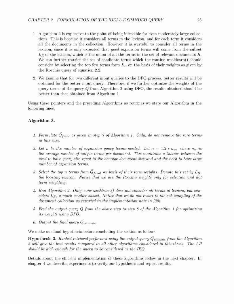
Algorithm 3.
1. Formulate ~Qfinal as given in step 7 of Algorithm 1. Only, do not remove the rare termsin this case.
2. Let n be the number of expansion query terms needed. Let n = 1.2 ∗ nw, where nw isthe average number of unique terms per document. This maintains a balance between theneed to have query size equal to the average document size and and the need to have largenumber of expansion terms.
3. Select the top n terms from ~Qfinal on basis of their term weights. Denote this set by LB,the boosting lexicon. Notice that we use the Rocchio weights only for selection and notterm weighting.
4. Run Algorithm 2. Only, now weaklearn() does not consider all terms in lexicon, but con-siders LB, a much smaller subset. Notice that we do not resort to the sub-sampling of thedocument collection as reported in the implementation note in [30].
5. Feed the output query Q from the above step to step 8 of the Algorithm 1 for optimizingits weights using DFO.
6. Output the final query ~Qultimate
We make our final hypothesis before concluding the section as follows
Hypothesis 3. Ranked retrieval performed using the output query ~Qultimate from the Algorithm3 will give the best results compared to all other algorithms considered in this thesis. The APshould be high enough for the query to be considered as the IEQ.
Details about the efficient implementation of these algorithms follow in the next chapter. Inchapter 4 we describe experiments to verify our hypotheses and report results.
CHAPTER 2. FORMULATION OF THE IDEAL EXPANDED QUERY 26
2.8 Predicting relative performance of queries with IEQ
The focus of all the preceding sections was the formulation of the Ideal Expanded Query(IEQ).However one of the major goals of this work was to predict the relative performances of QueryExpansion(QE) algorithms on a per query basis without explicitly retrieving documents. In thissection we describe how we propose to use the IEQ to predict relative performances of queries.In what follows we describe our main hypothesis about the correlation between the performanceof a query and its similarity with the IEQ and several metrics that can be used to measure thissimilarity.
The IEQ represents the best possible query for a given information need and collection to besearched. Therefore, given a candidate expanded query for the same information need, it isnatural to expect that higher the similarity between the candidate query and the ideal query,better is the performance of the candidate query. This leads us to make the following hypothesis.
Hypothesis 4. If for a particular information need expressed by the original query Qorig, Qidealbe the IEQ, sim() be a similarity metric between two vectors and q1, q2 be any two expandedqueries, then sim(Qideal, q1) > sim(Qideal, q2) implies retrieval performance of q1 is better thanthe retrieval performance of q2.
In making the above hypothesis we have assumed that ranked retrieval performance due toa query q, as measured by some evaluation metric, say MAP, increases monotonically withthe similarity between Qideal and q as measured by the similarity metric sim(). If the abovehypothesis is true, it clearly enables us to predict the relative performances of queries, based ontheir relative similarity with the IEQ. This is precisely the goal that we had set out to achieve.
The various definitions of sim() that we use are detailed below.
• Jaccard Index(j): sim (I,Q) = | I ∩ Q || I ∪ Q |
• Cosine similarity(c): sim (I,Q) =~I · ~Q
||~I|| · || ~Q||
• Kendall’s rank correlation(τ): sim (I,Q) = no of concordant pairs−no of discordant pairs12n(n−1)
• Spearman’s rank correlation(ρ): sim (I,Q) =∑
i(xi−x)(yi−y)√∑i(xi−x)2(yi−y)2
• Pearson’s correlation(r): sim (I,Q) =∑
i(Ii−I)(Qi−Q)√∑i(Ii−I)
2(Qi−Q)
2
I and Q are the ideal and candidate queries respectively. As and when required we representthem in their set, vector and ranked list notations. Ii and Qi are the weights of the ith rankedterms in the ideal and candidate queries respectively. xi and yi are these term weights convertedto ranks. Note that the difference between the last two definitions of sim() is that in one weuse the weights of the terms while in the other we use the ranks of the terms (calculated on thebasis of their weights). A concordant pair is a pair of two terms in Q whose relative order in Qis same as that in I. Similarly a discordant pair is a pair of two terms in Q whose relative orderin Q is the opposite of that in I.
CHAPTER 3
Efficient Implementation Details
In this chapter we provide brief details about the efficient implementation of the Algorithm 1and Algorithm 2. Particularly, both DFO and Boosting seem prohibitively expensive. Howeverin the following sections we show that careful pre-processing of certain data structures andpreservation of results allow for fast implementation of these algorithms. In section 3.1 wediscuss the general index data structures that we use. In the two other sections that follow webriefly discuss implementation of Algorithm 1 and Algorithm 2 with the main focus being onDFO and Boosting. Algorithm 3 does not introduce any new expensive steps of its own andhence its implementation is not discussed here.
3.1 Index Data Structures
The collection to be searched is indexed using the Terrier IR platform [24] developed by theUniversity of Glasgow. The human readable index files generated by Terrier and read into thefollowing run time data structures:
• lexicon An array containing the details of each unique term present in the collection. Thearray is indexed by the term-id and the details stored in each cell include the term, thedocument-frequency (df) and the term-frequency (tf).
• docids An array containing the details of each document present in the collection. The ar-ray is indexed by the document-id and the details stored in each cell include the document-name (docno), the number of unique terms in the document (docindexentrylength) andthe number of terms in the document (doclength).
• inverted-index An array indexed by term-id and containing the postings list for eachterm in the lexicon.
27
CHAPTER 3. EFFICIENT IMPLEMENTATION DETAILS 28
• rel-doc-list An array indexed by the query-id and containing the list of all relevant doc-uments for each query.
• offsets An array indexed by document-id. The cell corresponding to a particular docidcontains the offset into a binary file. The binary file, sometimes called the direct-index,contains the list of (term,frequency) pairs of all the unique terms present in all documents.The offset points to the location in this file from where the information pertaining to thedocument with id = docid is stored. Starting from this offset, exactly docindexentrylengthnumber of (term,frequency) pairs should be read to get the details of the document withdocument-id = docid.
These data structures are built once, at the start of the process and hence the build time is not ofinterest to us. Also these data structures do not need any insertions or deletions. Finally, sinceall searches into this data structures are done using either term-id, document-id or query-id,search time is O(1).
3.2 Implementing Algorithm 1
Steps 1 to 7 of Algorithm 1 are fairly straightforward and does not have much scope for impro-visation. The following are some details worth mentioning:
• Since we use raw term frequencies from the direct-index, we have to compute the Ltu orLnu weights each time they are required. For large collections, pre-computing and storingthem in memory for each document is infeasible. Also, retrieving them from a binary file,as is done with the direct-index, turned out to be more expensive.
• Using |L| dimensional vectors, where |L| is the lexicon size, as opposed to compact vectorscontaining just the required number of terms, proved very convenient time and again. Forcomputing the number of relevant documents in which each term occurs, we used a 0 ini-tialized |L| dimensional integer vector. For each term with id = term-id in each documentof the list rel-doc-list[query-id], we incremented the count of the term-idth component ofthe vector. If nr = |rel-doc-list[query-id]| and sr be the average size of documents in rel-doc-list[query-id] then running time complexity is O(nr * sr). This is faster than the otheralternative: for each term in the lexicon, for each document in the rel-doc-list[query-id] inwhich the term occurs, increment the count. Here the cost is O(|L| ∗ nr ∗ log sr)
• For the centroid ~Qrel, we construct it again in a 0 initialized |L| dimensional vector, byadding each of the Ltu weighted terms from the relevant documents present in the rel-doc-list[query-id], to its corresponding component in the vector, determined by the term-id.The Ltu weights were pre divided by the size of the list rel-doc-list[query-id] to avoidanother pass over the array, which would be expensive.
• For selecting the heaviest nw terms or the most similar max{ |C|100 , |R|} non relevant docu-ments, we used a min heap of (id,score) where the elements were compared on the basis oftheir scores. The maximum capacity ch of the heap was restricted to the target number of
CHAPTER 3. EFFICIENT IMPLEMENTATION DETAILS 29
elements to be selected ,i.e nw or max{ |C|100 , |R|}. As long as the heap was not full, elementswere inserted in it normally. When the heap became full, a new element was only insertedif it’s score was greater than the score of the element at the top of the heap. In that casethe old top element was replaced by the new element which was then bubbled down to itscorrect position.
Implementing step 8–DFO: The original DFO steps mentioned in Chapter 2 section 2.4 seemvery expensive. This is because for a change in weight of each term of the input query, we haveto score all the documents in collection, rank them and evaluate the result. Let us denote thesize of the query vector by |q|, average size of a document vector by |d| and the collection sizeby n. Then, time complexity of computing score of all documents using dot product similarityis O(n ∗ (|q|+ |d|)) and that of ranking is O(n ∗ log n). Therefore the time complexity of a singlepass in the original DFO is O(|q| ∗ (n ∗ (|q|+ |d|) + n ∗ log n)). However, once we have scored allthe documents in the collection on a query, subsequent change in term weight of a single termwill only affect the documents in which the term is present. More over the change will be onlydue to the contribution of the term whose weight has changed. These observations lead us torewrite the DFO steps as follows:
Modified DFO steps:
1. Initialize an empty data structure term-docid-map. For each term in q, term-docid-mapwill store a list of (i, wi) pairs where i is the id of a document in which the term occursand wi is the weight of the term in that document.
2. Create an enhanced version of the routine that calculates score of a document d on a queryq. Pass a pointer to term-docid-map to this routine. Enhance this routine by adding code,such that when q and d agree on a term, not only does the product of their weights getadded to their dot product sum, but the docid of d and the weight of this term in d getsadded in the bucket for the term in term-docid-map also.
3. Initially rank all the documents corresponding to the input query q by using the aboveenhanced score calculating routine. At the end of the ranking routine, this step willcompletely populate term-docid-map. Denote the average document frequency of terms interm-docid-map by n
′.
4. For each pass s
(a) Create a copy of the document scores. Document scores are read from the originalcopy but all changes in document scores are written on this duplicate copy.
(b) For each term t in q
i. Let incr be the increment in t’s weight for round s.
CHAPTER 3. EFFICIENT IMPLEMENTATION DETAILS 30
ii. For each document d in term-docid-map[t]
A. let w be the weight of t in d.
B. new-score-of-d = old-score-of-d + incr ∗ w.
iii. Rank all the documents and compute the AP. Revert all changes made in thequery term weights and document scores. Only if AP improves, remember thechange.
(c) Effect all remembered changes in the original query. Overwrite the original documentscores by the copy.
Observe that in the above algorithm we are not re-scoring all n documents, but only n′documents
and it can be expected that n′<< n. Also for a given d and q, updating the score in step 4.(b)
ii. B) takes O(1) time. Therefore time complexity for a single pass the above algorithm isO(|q| ∗ (n
′+ n ∗ log n)) which is clearly an improvement over the earlier case. So much, that we
can afford to experiment with 5 DFO passes instead of the standard 3 DFO passes mentionedin [8]
3.3 Implementing Algorithm 2
As with the case with DFO, the adaptation of the AdaBoost algorithm in chapter 2 section 2.6is prohibitively expensive. Though Algorithm 2 seems innocuous, it is the call to weaklearn()in step 3.a) that spells trouble. Let l = |L| be the size of the entire lexicon and n be the totalnumber of documents in the collection. Then, the weaklearn() subroutine has a running timecomplexity of O(l ∗n), which is practically infeasible even on moderately large collections. How-ever we observe that good expansion terms are likely to come only from the relevant documents,and that step 3 requires only the the list of documents misclassified by a term. This list can bepre-computed and reused each time it is needed. These observations lead us to implement thealgorithm in the following way.
Pre-processing
1. Construct the union LR;LR ⊆ L, of all terms in the set R of relevant documents stored inrel-doc-list [query-id].
2. Construct the misclassified-doc-list data structure which stores, for each term in LR, a listof docids of documents in the collection C that is mis-classified by the term. This list canbe easily constructed using the rel-doc-list [query-id], represented by the set R, and theposting list for the term id, represented by I and stored in inverted-list [term-id]. Then themisclassified-doc-list = (R− I) ∪ (I −R)
CHAPTER 3. EFFICIENT IMPLEMENTATION DETAILS 31
Modified weaklearn()
1. Consider all terms t in LR
2. For each term t design a hypothesis h(t) such thatt ∈ d =⇒ d is relevant.t /∈ d =⇒ d is not relevant.
3. Denote the misclassified doc list by the set M and calculate error as
εs(t) =∑
i:di∈MDs(i).
4. Choose the term t which minimizes min{εs, 1− εs}
Let l′
= |LR| and n′
= |M |. Then the above implementation of weak learn has running timecomplexity O(l
′ ∗ n′). Since l
′ � l and n′ � n, the modified weaklearn() should be much faster
that the original one.
With these implementations Algorithm 1 runs in ≈ 3 minutes per query, Algorithm 2 runs in≈ 1.2 minutes per query and Algorithm 3 runs in ≈ 4.5 minutes per query on a Intel Corei3processor with 2GB of RAM. Given that we do 5 passes of DFO this is reasonably fast.
CHAPTER 4
Results and Discussions
In this chapter we describe our experiments and report results obtained on standard test collec-tions. We start out by detailing our experiments and mentioning the hypotheses that they aredesigned to test in section 4.1. Results pertaining to the Ideal Expanded Query are reportedin section 4.2, while those pertaining to the results of prediction using the IEQ are reported insection 4.3.
4.1 Experiment Design
There are 4 hypotheses in this dissertation. Hypotheses 1 to 3 deal with the Ideal ExpandedQuery. Hypothesis 4 deals with the prediction of relative performances of queries using theIEQ. In what follows, subsection 4.1.1 describes the experiments and collections used for testinghypotheses dealing with IEQ while subsection 4.1.2 does the same for the hypothesis dealingwith the predictive power of the IEQ.
4.1.1 Testing the IEQ
We run Algorithms 1, 2 and 3 on the 50 queries of the TREC8 adhoc track; query number 401to 450. The collection we search is disks 4 & 5 of the standard TREC collection (excluding theCongressional Records sub-collection on Disk 4).
For each algorithm, the set of 50 expanded queries so produced are used to perform retrieval us-ing the Terrier IR platform, by turning off all kinds of query expansion and query term weightingfeatures inbuilt into Terrier. We evaluate the retrieval result using MAP for 4 different docu-ment term weighting schemes; BM25, DLH13, InL2 and TF-IDF. The baseline retrieval system
32
CHAPTER 4. RESULTS AND DISCUSSIONS 33
against which we compare our method is the BM25 implementation provided by Terrier usingBo1 query expansion. High MAP values for Algorithm 1 and Algorithm 3 will verify theircorresponding hypothesis. We do not explicitly test hypothesis 2 since better performance ofAlgorithm 3 over Algorithm 1 will verify it indirectly. Also small or negligible variance acrossdifferent document weighting schemes will verify that the performance of the queries producedby the algorithms are independent of the document weighting and retrieval model.
To better bring out the relative performances of Algorithms 1, 2 and 3 and their overall superi-ority w.r.t our baseline retrieval system, we compare their performances on 10 queries from theTREC8 adhoc track that register very poor AP with our Baseline retrieval scheme.
4.1.2 Testing predictive power of IEQ
Hypothesis 4 deals with the predictive power of the IEQ formulated by us. For this we use thequery produced by Algorithm 3 as the IEQ. The candidate queries whose relative performancesare to be predicted are implementations of the LCA, KLD and RBLM query expansion algo-rithms introduced in Chapter 1 section 1.2 and their various parameter variations1. To measurethe similarity between the IEQ and the candidate queries we use 5 different similarity measures;Jaccard index, cosine similarity, Pearson’s correlation coefficient, Kendall’s rank correlation andSpearman’s correlation. We select three different sets of queries for performance prediction (pre-diction to be made for the queries in each set separately). All queries in the first set have 5expansion terms. Since all queries have the same number of terms, variation in prediction perfor-mance due to number of expansion terms is nullified. We select 20 queries into this set (10 fromLCA and 10 from KLD; no RBLM run with 5 expansion terms is available to us). We obtain 5different rankings of this set based on the similarity scores obtained with each of the 5 similaritymeasures. We then observe the correlation (pearson, kendall and spearman) of these rankingswith their actual ranking based on their retrieval performances which are already documented.High positive correlation will indicate successful prediction and hence will verify Hypothesis 4.In the second set, all queries have 50 expansion terms. We select 21 queries into this set(10 fromKLD, 10 from LCA and 1 from RBLM because ony 1 RBLM run having 50 expansion terms isavailable to us). In set 3, queries have different number of expansion terms(varies from 5 to 50).We select 31 queries into this set(1 from RBLM and 15 each from from KLD and LCA; these 15were chosen as follows–for each odd multiple mo of 5 between 5 to 50, select one query havingmo expansion terms, for each even multiple me of 5 between 5 and 50, select 2 queries havingme expansion terms). These three sets were so chosen in order to explore any dependence ofprediction accuracy on the number of expansion terms of the candidate queries. We repeat forset 2 and 3, the same procedure that was applied for set 1.
1these implementations and evaluationswere carried out by Mrs. Dipasree Pal andothers at the IR Lab, ISI Kolkata.
CHAPTER 4. RESULTS AND DISCUSSIONS 34
4.2 Results for IEQ
Table 4.1 presents the retrieval performance of the expanded queries produced by Algorithm 1for 4 different document weighting schemes. The MAP hovers around 0.77 for all 4 differentdocument weighting models and hence results obtained are highly independent of the retrievalmodel. Though Hypothesis 1 stands verified, results are not high enough to term the queryproduced by Algorithm 1 as the IEQ.
Algorithm 1: Query Zoned Rocchio Query with DFO
Weighting Model Queries Baseline MAP IEQ MAP percentage increase
BM25 TREC8(401-450) 0.2610 0.7710 195%
DLH13 TREC8(401-450) 0.2747 0.7724 181%
InL2 TREC8(401-450) 0.2672 0.7760 190%
TF-IDF TREC8(401-450) 0.2637 0.7730 193%
Table 4.1: MAP values obtained for Algorithm 1
Similarly, Table 4.2 presents the results obtained using Algorihm 2 with all column and rowdefinitions similar to that of Table 4.2. The results are yet again independent of the documentweighting schemes. However the retrieval performance is about 18% lower than that of Algo-rithm 1. Hence Boosting terms selected using Rocchio query is not a good choice for formulatingthe IEQ. However, it should be noted that Algorithm 2 does not employ DFO which is knownto increase query term weighting quality considerably. Still it manages to achieve a averageMAP ≈ 0.63. Hence the quality of terms selected by this algorithm is better than the qualityof terms selected at the end of step 7 in Algorithm 1 and retrieval performance should improveconsiderably on application of DFO to the query terms selected by Algorithm 2. ThereforeHypothesis 2 is true with very high probability, though we do not test it explicitly.
Algorithm 2: Boosting with Query Zoned Rocchio query
Weighting Model Queries Baseline MAP IEQ MAP percentage increase
BM25 TREC8(401-450) 0.2610 0.6196 137%
DLH13 TREC8(401-450) 0.2747 0.6527 137%
InL2 TREC8(401-450) 0.2672 0.6314 136%
TF-IDF TREC8(401-450) 0.2637 0.6213 135%
Table 4.2: MAP values obtained for Algorithm 2
Table 4.3 presents the retrieval performance obtained using the Algorithm 3. The MAPs ob-tained are around 0.81 for all the 4 document weighting schemes used. This clearly verifies bothHypothesis 2 and Hypothesis 3 at the same time. Also, it brings out the effectiveness of the 5pass DFO used by us, since it effected a 28.5% improvement over Algorithm 2. The MAP ishigh enough for the queries produced by Algorithm 3 to be considered as the IEQ.
CHAPTER 4. RESULTS AND DISCUSSIONS 35
Algorithm 3: DFO applied to Boosting with Query Zoned Rocchio query
Weighting Model Queries Baseline MAP IEQ MAP percentage increase
BM25 TREC8(401-450) 0.2610 0.8110 210%
DLH13 TREC8(401-450) 0.2747 0.8258 200%
InL2 TREC8(401-450) 0.2672 0.8181 206%
TF-IDF TREC8(401-450) 0.2637 0.8132 208%
Table 4.3: MAP values obtained for Algorithm 3
Table 4.4 compares the relative performances of the three algorithms used by us on 10 difficult-to-retrieve queries, as attested by the low MAP obtained using the baseline retrieval methoddescribed at the start of the chapter. Compared to Algorithm 1, Algorithm 3 performs betteron most of the queries while being marginally worse on a few. Since Algorithm 3 is equivalentto DFO applied to the output of Algorithm 2, this comparison proves the superiority of termselection using Algorithm 2, i.e. Boosting from a pool of terms short-listed on the basis of theRocchio weights.
Query Number Baseline AP Algorithm-1 AP Algorithm-2 AP Algorithm-3 AP
401 0.0279 0.6725 0.5820 0.6656
413 0.0460 0.7920 0.6264 0.8346
421 0.0220 0.3804 0.1631 0.5288
426 0.0543 0.6578 0.5815 0.6943
432 0.0011 0.8006 0.5674 0.9621
433 0.0043 1.0000 1.0000 1.0000
437 0.0176 0.5737 0.2870 0.7252
439 0.0592 0.5153 0.3659 0.5548
442 0.0119 0.6943 0.5692 0.8117
448 0.0070 0.7115 0.3482 0.7023
Table 4.4: Performance on difficult-to-retrieve queries
4.3 Results for prediction using IEQ
The 5 rows in the following tables correspond to the different similarity measures used to com-pute the similarity between the IEQ and the candidate query, while each of the 3 columns denotethe different measures of correlation between the actual ranking of runs and the predicted rank-ing of the runs.
Table 4.5 represents the data for a set of 31 different parameter variations of 3 different QEalgorithms. An element of this 31-element set is actually a set of 50 expanded queries, obtainedby a certain parameter setting of a certain QE algorithm acting on the 50 queries from the
CHAPTER 4. RESULTS AND DISCUSSIONS 36
Pearson Kendall Spearman
Jaccard index 0.350437 0.130963 0.183748
Pearson 0.578621 0.286329 0.389483
Kendall −0.002708 −0.072504 −0.113027
Spearman −0.003438 −0.058723 −0.097622
cosine 0.642448 0.289576 0.388241
Table 4.5: Correlation between actual ranking and predicted ranking for 31-element-set
TREC8 adhoc track. They act as the candidate expanded queries whose performances we try topredict. Henceforth we refer to this set as the 31-element-set. The number of expansion termsin the elements of the 31-element-set varies from 5 to 50. The results reported in Table 4.5 arethe average correlations between the actual ranking of the elements of the 31-element-set andthe predicted ranking, where the average is over the 50 queries. It is immediately clear thatcosine similarity between the IEQ and the candidate queries is the best predictor of the actualrelative performances between the queries.
Pearson Kendall Spearman
Jaccard index 0.403195 0.177873 0.237410
Pearson 0.502687 0.231794 0.293571
Kendall −0.283837 −0.097530 −0.164953
Spearman −0.277611 −0.108700 −0.183090
cosine 0.515466 0.201074 0.254903
Table 4.6: Correlations for the 20-element-set. Expanded Queries have 5 terms.
To explore the possible effect of the number of query terms on the accuracy of our predictedranking, we report the results obtained for runs containing queries having the same number ofexpansion terms. Table 4.6 presents the results for a set of 20 different parameter variationsof 2 different QE algorithms, where each expanded query has only 5 terms. Similarly table 4.7presents the results for a set of 21 different parameter variations of 3 different QE algorithmswhere each query has 50 expansion terms.
Pearson Kendall Spearman
Jaccard index 0.537169 0.198639 0.267029
Pearson 0.611369 0.265306 0.349775
Kendall −0.162379 −0.054227 −0.083143
Spearman −0.263758 −0.104762 −0.166578
cosine 0.673141 0.296599 0.380705
Table 4.7: Correlations for the 21-element-set. Expanded Queries have 50 terms.
CHAPTER 4. RESULTS AND DISCUSSIONS 37
Results show that agreement is better in the case where queries have 50 expansion terms. Thissuggests that higher the number of intersections of the candidate queries with the IEQ, betteris the quality of the prediction. Predictions on candidate queries containing 100 or 150 termscan be investigated in future to study this possibility. Also the number of terms in the querieswhich are not present in the ideal query can influence the prediction quality. To investigate suchpossibility, prediction quality on synthetic queries that are randomly sampled proper subsetsof the IEQ can be computed. Higher correlation than what is reported here will confirm thedependence of the prediction quality on the number of intersecting terms.
CHAPTER 5
Conclusion
We had two clear goals to achieve in this dissertation. First was the formulation of the Ideal Ex-panded Query(IEQ) by selecting a set of good expansion terms. The results clearly indicate thatour most important hypothesis in this regard, hypothesis 3, stands verified. Retrieval usingour formulated IEQ had MAP > 0.8 across several different document weighting and retrievalmodels. However most of the algorithms used by us are fairly old. Suitability of more recentalgorithms for this purpose can be investigated in future. Moreover few modifications can bemade to the basic DFO framework to push the AP close to 1, albeit at the risk of over-fitting.For example, we could add, and assign high weights, to terms from relevant documents that arevery low in the ranked list even after a few DFO passes. Further research is necessary to as-certain the extent to which such enhancements translate into better predictive power of the IEQ.
Our second goal was to investigate if we could use the IEQ in some way to predict the relativeperformances of queries. Again our most important hypothesis in this regard, hypothesis 4, isverified to a large extent. Results indicate that cosine similarity between the input query andthe IEQ is the best similarity metric since it exhibits high correlation(pearson) with the MAPof the actual retrieval runs of the queries, and ranking runs based on their cosine similarity withthe IEQ show positive rank correlation with the actual ranking of the runs.
To conclude the dissertation we summarize our result in the following statement. The rankingof queries based on their cosine similarity with the Ideal Expanded Query producedby Algorithm 3 is a reasonable approximation of their actual relative retrievalperformances.
38
Bibliography
[1] Conference and labs of the evaluation forum (formerly known as cross-language evaluationforum). http://clef2012.org/.
[2] Forum for information retrieval evaluation. http://www.isical.ac.in/~fire/.
[3] Text retrieval conference. http://trec.nist.gov/.
[4] SIGIR ’98: Proceedings of the 21st Annual International ACM SIGIR Conference on Re-search and Development in Information Retrieval, August 24-28 1998, Melbourne, Aus-tralia. ACM, 1998.
[5] Gianni Amati and C. J. van Rijsbergen. Probabilistic models of information retrieval basedon measuring the divergence from randomness. ACM Trans. Inf. Syst., 20(4):357–389, 2002.
[6] Lourdes Araujo and Joaquın Perez-Iglesias. Training a classifier for the selection of goodquery expansion terms with a genetic algorithm. In IEEE Congress on Evolutionary Com-putation, pages 1–8. IEEE, 2010.
[7] Nicholas J. Belkin and W. Bruce Croft. Information filtering and information retrieval:Two sides of the same coin? Commun. ACM, 35(12):29–38, 1992.
[8] Chris Buckley and Gerard Salton. Optimization of relevance feedback weights. In Edward A.Fox, Peter Ingwersen, and Raya Fidel, editors, SIGIR, pages 351–357. ACM Press, 1995.
[9] Claudio Carpineto, Renato de Mori, Giovanni Romano, and Brigitte Bigi. An information-theoretic approach to automatic query expansion. ACM Trans. Inf. Syst., 19(1):1–27, 2001.
[10] Hui Fang. A re-examination of query expansion using lexical resources. In Kathleen McK-eown, Johanna D. Moore, Simone Teufel, James Allan, and Sadaoki Furui, editors, ACL,pages 139–147. The Association for Computer Linguistics, 2008.
39
BIBLIOGRAPHY 40
[11] Hui Fang and ChengXiang Zhai. An exploration of axiomatic approaches to informationretrieval. In Ricardo A. Baeza-Yates, Nivio Ziviani, Gary Marchionini, Alistair Moffat, andJohn Tait, editors, SIGIR, pages 480–487. ACM, 2005.
[12] Hui Fang and ChengXiang Zhai. Semantic term matching in axiomatic approaches toinformation retrieval. In Efthimis N. Efthimiadis, Susan T. Dumais, David Hawking, andKalervo Jarvelin, editors, SIGIR, pages 115–122. ACM, 2006.
[13] Yoav Freund and Robert E. Schapire. A decision-theoretic generalization of on-line learningand an application to boosting. J. Comput. Syst. Sci., 55(1):119–139, 1997.
[14] George W. Furnas, Thomas K. Landauer, Louis M. Gomez, and Susan T. Dumais. Thevocabulary problem in human-system communication. Commun. ACM, 30(11):964–971,1987.
[15] Debasis Ganguly. Implementing a language modelling framework for information retrieval.Master’s thesis, Indian Statistical Institute, 2008.
[16] Parantap Goswami. Query expansion using wordnet. Master’s thesis, Indian StatisticalInstitute, 2011.
[17] Donna Harman. Overview of the fourth text retrieval conference (trec-4). In TREC, 1995.
[18] Ben He and Iadh Ounis. Studying query expansion effectiveness. In Mohand Boughanem,Catherine Berrut, Josiane Mothe, and Chantal Soule-Dupuy, editors, ECIR, volume 5478of Lecture Notes in Computer Science, pages 611–619. Springer, 2009.
[20] J.J.Rocchio. Relevance feedback in information retrieval. In The SMART Retrieval System-Experiments in Automatic Document Processing, pages 313–323. Prentice Hall, Inc., Engle-wood Cliffs, NJ, 1971.
[21] Victor Lavrenko and W. Bruce Croft. Relevance-based language models. In W. BruceCroft, David J. Harper, Donald H. Kraft, and Justin Zobel, editors, SIGIR, pages 120–127.ACM, 2001.
[22] Dekang Lin. An information-theoretic definition of similarity. In Jude W. Shavlik, editor,ICML, pages 296–304. Morgan Kaufmann, 1998.
[23] Christopher D. Manning, Prabhakar Raghavan, and Hinrich Schutze. Introduction to in-formation retrieval. Cambridge University Press, 2008.
[24] I. Ounis, G. Amati, V. Plachouras, B. He, C. Macdonald, and C. Lioma. Terrier: AHigh Performance and Scalable Information Retrieval Platform. In Proceedings of ACMSIGIR’06 Workshop on Open Source Information Retrieval (OSIR 2006), 2006.
[25] Jose R. Perez-Aguera and Lourdes Araujo. Comparing and combining methods for auto-matic query expansion. CoRR, abs/0804.2057, 2008.
BIBLIOGRAPHY 41
[26] Jay M. Ponte and W. Bruce Croft. A language modeling approach to information retrieval.In SIGIR [4], pages 275–281.
[27] M. Porter. An algorithm for suffix stripping. Program, 14(3):130–137, 1980.
[28] Stephen E. Robertson and Hugo Zaragoza. The probabilistic relevance framework: Bm25and beyond. Foundations and Trends in Information Retrieval, 3(4):333–389, 2009.
[29] Gerard Salton, A. Wong, and C. S. Yang. A vector space model for automatic indexing.Commun. ACM, 18(11):613–620, 1975.
[30] Robert E. Schapire, Yoram Singer, and Amit Singhal. Boosting and rocchio applied to textfiltering. In SIGIR [4], pages 215–223.
[31] Amit Singhal. At&t at trec-6. In TREC, pages 215–225, 1997.
[32] Amit Singhal. Modern information retrieval: A brief overview. IEEE Data Eng. Bull.,24(4):35–43, 2001.
[33] Amit Singhal, Mandar Mitra, and Chris Buckley. Learning routing queries in a query zone.In SIGIR, pages 25–32. ACM, 1997.
[34] Ellen M. Voorhees and Donna K. Harman, editors. TREC: Experiment and Evaluation inInformation Retrieval. The MIT Press, Cambridge, 2005.
[35] Jinxi Xu and W. Bruce Croft. Improving the effectiveness of information retrieval withlocal context analysis. ACM Trans. Inf. Syst., 18(1):79–112, 2000.