McMaster Universit yDigitalCommons@McMaster Open Access Dissertations and Theses Open Dissertations and Theses 10-1-2011 Condition Monitoring for Rotational MachineryDaniel C. Volante McMaster University , [email protected]This Thesis is brought to you for free and open access by t he Open Dissertations and Theses at DigitalCommons@McMaster. It has been accepted for inclusion in Open Access Dissertations and Theses by an authorized administrator of DigitalCommons@McMaster. For more information, please contact [email protected]. Recommended Citation Volante, Daniel C., "Condition Mo nitoring for R otational Machinery " (2011). Open Access Dissertations and Theses. Paper 6105. http://digitalcomm ons.mcmaster .ca/opendissertati ons/6105
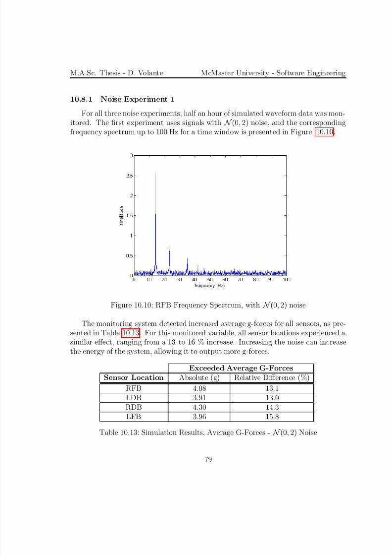
Recommended Citation Volante, Daniel C., "Condition Monitoring for Rotational Machinery" (2011). Open Access Dissertations and Theses. Paper 6105.http://digitalcommons.mcmaster.ca/opendissertations/6105
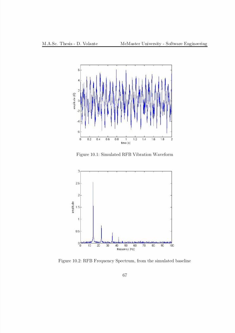
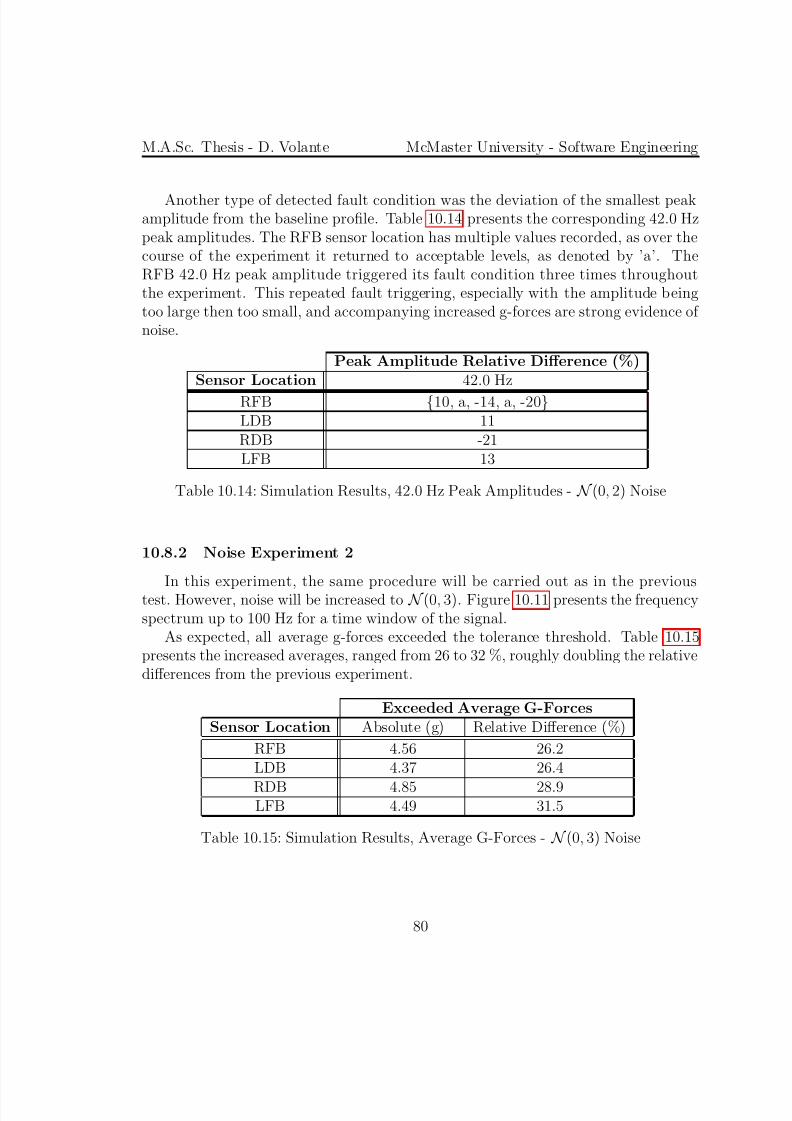
Vibrating screens are industrial machines used to sort aggregates through theirhigh rotational accelerations. Utilized in mining operations, they are able to screendozens of tonnes of material per hour. To enhance maintenance and troubleshoot-ing, this thesis introduces a vibration based condition monitoring system capable of observing machine operation. Using acceleration data collected from remote parts of the machine, software continuously detects for abnormal operation triggered by faultconditions. Users are to be notified in the event of a fault and be provided with
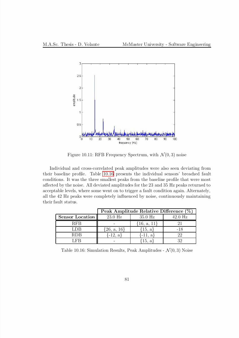
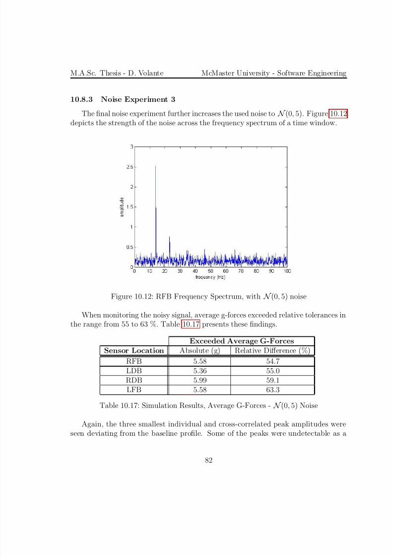
relevant information.Acceleration data is acquired from a set of sensor devices that are mounted tospecified points on the vibrating screen. Data is then wirelessly transmitted to acentralized unit for digital signal processing. Existing sensor devices developed fora previous project have been upgraded and integrated into the monitoring system.Alternative communication technologies and the utilized Wi-Fi network are examinedand discussed.
The condition monitoring system’s hardware and software was designed followingengineering principles. Development produced a functional prototype system, imple-menting the monitoring process. The monitoring technique utilizes signal filtering andprocessing to compute a set of variables that reveal the status of the machine. Decision
making strategies are then employed as to determine when a fault has occurred.Testing performed on the developed monitoring system has also been documented.
The performance of the prototype system is examined as different fault scenariosare induced and monitored. Results and descriptions of virtual simulations and liveindustrial experiments are presented. The relationships between machine faults anddetected fault signatures are also discussed.
I would first like to express my gratitude to my supervisor Dr. Martin v. Mohren-schildt. His guidance and expertise has provided me opportunity to further developmy engineering experience. I would also like to thank my examination committee,Dr. Khedri and Dr. Leduc, for providing me with additional feedback and insight.
I want to acknowledge the engineers and technicians at the sponsoring company.Their industrial knowledge was vital not only to my work, but also in my professionalgrowth.
A special thanks to Dr. Jay Parlar, whose original work was the foundation onwhich I have built. I also want to thank all the graduate students who resided inITB 135, as they have offered companionship and encouragement over the years.
Finally, I would like to gratefully thank my significant other, Brianne Nicholls.Her love and support has keep me grounded throughout my studies and has allowedme to flourish.
M.A.Sc. Thesis - D. Volante McMaster University - Software Engineering
1 Introduction
1.1 Thesis Motivation
Vibrating screens are industrial machines used to sort aggregates through theirhigh rotational accelerations. Utilized in mining operations, they are able to screendozens of tonnes of material per hour. McMaster University’s Department of Com-puting and Software was approached by a manufacture of these machines to developtheir next generation of vibration analysis tool. The tool was designed to aid techni-cians in both maintenance and fault detection of rotating machinery [21]. After fouryears of development, the product was a system able to measure and analyze three
axes of vibration data from eight simultaneous sensors. Technicians are presentedwith numerical and graphical data on the machine’s operation in real time. A postprocessing software package was also constructed for further analysis.
With the initial project a success, the company wants to expand its vibrationanalysis tool into a permanently installed condition monitoring system. The newsystem is intended to monitor the operation of a vibrating screen and notify users whenabnormal operation or faults are detected. This would warn users of malfunctions andimpending failure events before machines becomes inoperable. Instead of relying onreactionary troubleshooting for maintenance, the vibrating screens would be activelymonitored.
It is the intention of the thesis to take the acquired knowledge from the existingvibration analysis tool and apply it to condition monitoring. Previously developedelectronics and software strategies are to be modified and integrated into the project.Additional software is to be developmed to complete the remainder of the monitoringsystem.
1.2 Thesis Objective
The goal of this thesis is to develop and construct an actual condition monitoringsystem for use on vibrating screens. The system should be able to acquire accelerationdata from specified points on a vibrating screen and transmit it to a centralized
processing unit. Waveform data is to be filtered so that monitored variables can becalculated, such as peak frequencies and average g-forces. The monitored variableswill then be compared against the baseline profile. The baseline is observed when thevibrating screen is in good health, and its profile is to be comprised of the variables.
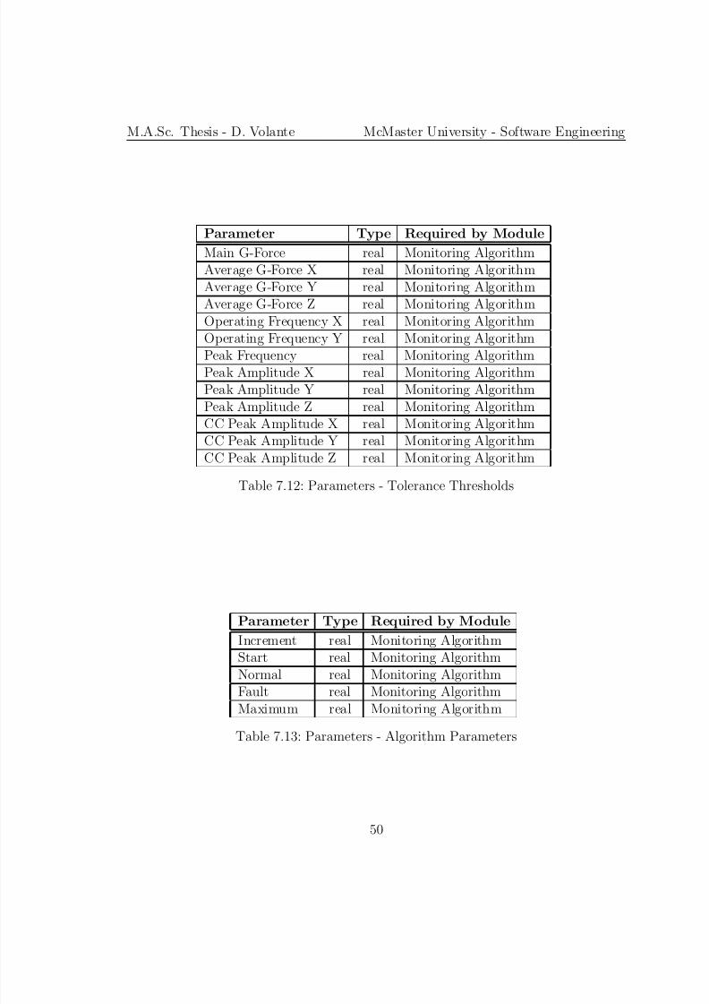
Monitored variables that deviate from the baseline profile would be indicators of undesired operation or machine faults. Users will specify tolerance thresholds on the
M.A.Sc. Thesis - D. Volante McMaster University - Software Engineering
monitored variables and algorithms are used to determine when a fault has occurred.When a machine fault is identified, users are to be notified. The system is alsoto record vibration data in periodic intervals, as well as data that triggers a faultcondition.
In summary, the condition monitoring system should be capable of the following:
• acquire synchronized acceleration data from a set of measurement locations
• detect short time and sustained machine abnormalities by examining vibrationwaveforms and corresponding frequency content
• notify users of abnormal operation and specify the triggered fault condition
• periodically record the monitored vibration data, and record data pertaining tofault events
1.3 Contributions
Contributions provided this thesis support the completion of the thesis objectivein constructing a condition monitoring system for vibrating screens. The followinglist separates the contributions into individual components:
• design and assemble the hardware for a permanently installed monitoring system• design and implement software to execute continuous condition monitoring
• system assesment through virtual simulations and live industrial experiments
1.4 Assumptions
The thesis and corresponding condition monitoring system have the following as-sumptions:
• frequencies of interest appear as resonance frequencies and peak-like in nature
• vibrating screens are subject to Gaussian noise, which is mainly due to materialflow
M.A.Sc. Thesis - D. Volante McMaster University - Software Engineering
2 Literature Review
2.1 Condition Monitoring
Condition monitoring is a maintenance technique that monitors the condition orhealth of machinery or structures and advises when upkeep is necessary. It consistsof collecting system data through sensor equipment and then processing it into mean-ingful information. Decision making strategies are then employed to determine whenmaintenance is required [12]. Fault diagnoses is at the core of condition monitor-ing. Implemented techniques are utilized to detect fault conditions and even identifyspecific machines faults.
Due to the wide variety of systems, the literature on condition monitoring is verydiverse. Condition monitoring is widespread in industry, with applications in automa-tion, predictive maintenance and quality control [17]. Monitoring has been developedfor motors [13, 19], circuit breakers [10], cantilever structures [4], individual bearingcomponents [20,32] and various other machinery [15,25, 28]. System information canbe extracted from various types of collected data: electrical, vibrational, thermal,environmental, results from oil analysis, etc. [12]. However, as this project focuseson monitoring rotational machinery, vibration data will prove the most valuable. Asstated by researchers from the Buckinghamshire Chilterns University College,
Vibration is probably the most important indicator of the mechanical in-tegrity of rotating machinery. Like the heartbeat of humans, vibrationwithin rotating machinery tells a great deal about the health of that ma-chinery. Machinery health monitoring, through condition monitoring, candetect faults before they become serious, optimize maintenance activitiesduring planned shutdowns and unscheduled outages. [17]
With the recent advances in micro-machining, it is possible to purchase low costacceleration sensors as to construct remote vibration monitoring devices [34]. Multiplesensors have proved to be much more useful, as a single sensor cannot provide enoughdata when monitoring a complex system [12]. Understanding the relationships be-
tween multiple sets of signals reveals even more information for fault diagnostics [25].Another consideration of condition monitoring is whether to monitor the target
system continuously or periodically. Currently, the most common practice is to mon-itor in periodic intervals [35]. By choosing to use less data, it is possible to utilizeadvanced filtering techniques combined with detailed analysis to ensure accurate di-agnostics [12]. Models have even been developed to optimize the monitoring intervals
M.A.Sc. Thesis - D. Volante McMaster University - Software Engineering
through cost functions [9, 35]. Another technique determines the monitoring inter-val given the system’s risk of failure [8]. Any periodic monitoring, however, has thepossibility to miss failure events which could provide insight on the correspondingfault.
Accordingly, an obvious advantage of continuous monitoring is being able to ob-serve all the failure events. In one particular project, the authors wanted to expandthe periodic monitoring of a circuit breaker with continuous vibration based monitor-ing [10]. A clear expectation of the continuous monitoring system was that it musthave a false alarm rate much lower than the targeted system’s failure rate. Noiseproved to be the most challenging issue causing numerous spikes. A proposed method
of fast noise filtering was to ignore the vibrations where the existence of noise is pre-defined. Additionally, a hardware solution suggested the use of differential amplifiersto reduce system noise.
Continuous monitoring projects have been utilizing modern computing, and areoptimizing analysis with respect to resolution, frequency bands and computationalcomplexity. Some of these systems are able to monitor rotating machinery by lookingfor specific indicators of faults [5, 36]. Another monitoring project implemented acontinuous wavelet transform, a detailed yet expensive analysis [17]. Development wasspent trading off accuracy and frequency ranges for reduce computational complexity.To compensate for the accuracy loss, additional signal enhancing techniques wereintroduced, primarily chosen for their high efficiency.
2.2 Fault Diagnoses
Fault diagnoses is used to detect and identify machine faults. The first step,fault detection, is used to generate an alarm signal when a fault condition has beenbreached. This is accompanied by fault isolation and identification; processes whichattempt to determine the source and severity of the fault [30].
Machines operating with faults can have reduced efficiency and even accelerateddeterioration leading to system failure. Faults can be classified as intermittent orpermanent. Intermittent faults persists for a bounded period of time, although canalter system operation after their presence subsides. Once permanent faults manifest,they continue to exist until maintenance is performed [30].
A review on fault diagnoses is presented, divided into four categories. Techniquesare classified into signal-based diagnoses, model-based diagnoses, neural network-based diagnoses, and expert systems.
M.A.Sc. Thesis - D. Volante McMaster University - Software Engineering
2.2.1 Signal-Based Diagnoses
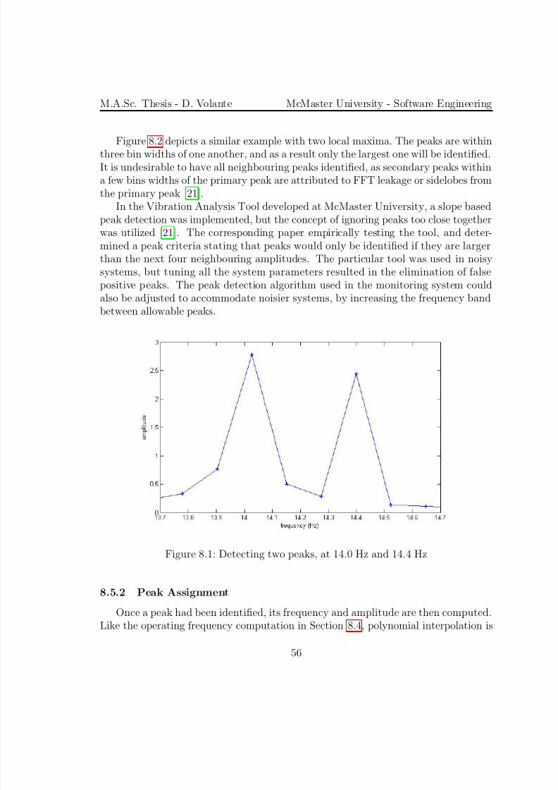
Signal-based fault diagnoses is the most traditional approach to fault detection.It relies on signal processing of system measurements and its comparison against nor-mal operational trends [30]. Especially in vibration based fault detection, waveformanalysis is the most common form of data interpretation. Standardized forms of equa-tions and processing techniques can allow the calculation of recognized variables. Thethree main categories of waveform analysis are time domain, frequency domain andtime-frequency analysis [12].
Different characteristics can describe a time domain waveform such as period,peak, mean and standard deviation [13]. Higher order statistics such as root-mean-
square, skewness and kurtosis have been used as well [12]. All of these reveal differentaspects of the waveform, however are generally unable to extract all underlying signalinformation.
Frequency domain analysis begins by converting a time domain waveform into itsfrequency domain equivalent. The most common means of conversion is through thefast Fourier transform (FFT), as it can perform the transform with ease [5]. Oncethe frequency spectrum is available, it is then possible analyze to the entire signalor specific frequency regions of interest. With the use of peak detection, dominantfrequencies can be identified and singled out for further analysis [ 5]. When the dom-inant frequencies of a system have been established, special attention is given to any
other emerging frequency content, as it is likely to be the signature of fault. Envelopeanalysis is the most utilized technique in cases where the fault frequencies are allknown or pre-estimated [20]. However, it is not suitable to monitor a wide frequencyspectrum or a vibration spectrum when the signal-to-noise ratio is low. Additionalcharacteristics observable in the frequency spectrum are the spacing of sidebands, andthe presence of harmonics.
Time-frequency analysis combines both the time domain waveform and the cor-responding frequency spectrum. This enables the examination of transient features,such as impacts and fault events, as well the ability to monitor frequency contentover time [12]. As a result, time-frequency analysis is the most popular method fornon-stationary signals [25]. The Short-time Fourier transform (STFT) is a common
technique, where the signal is divided up into short-time segments, and then a FFTis applied to each window [12]. It is computationally efficient, however it providesconstant resolution for all frequencies in the window [17]. This makes it difficultto examine both low and high frequency content with high resolution. The Wigner-Ville distribution (WVD) overcomes this resolution limitation, however it suffers frominterference terms forced by the transform itself [12]. This can lead to difficult in-
M.A.Sc. Thesis - D. Volante McMaster University - Software Engineering
terpretation of the analysis. Improved transforms, such as Choi-Willams distributionand cone-shaped distribution, have been developed to further advance time-frequencyanalysis [25]. Taken together, while each transform is designed to excel in a specificmanner, the required trade-off to do so limits another merit.
The wavelet transform is another form of time-frequency analysis that has beenreceiving much attention. Like the STFT, the wavelet transform is able to converttime domain waveforms into frequency content over time by use of windowing. Con-versely, the wavelet transform uses variably size windows, allowing for the acquisitionof better resolutions. [20]. Large time windows are used to obtain precise resolutionfor low frequencies, while shorter windows give precise time information for high fre-
quencies. The wavelet transform has also received praise for its ability to reduce noisein raw signals [12].With modern instrumentation and control systems technology, vast amounts of
system data can be collected for analysis. While systems can be data rich, theycan also be information poor [18]. In these situations, feature extraction techniquesare used to deal with excessive amounts of redundant data. One of the most widelyused forms of feature extraction is Qualitative trend analysis (QTA). This data-driventechnique works by first extracting important features or trends from measurementsignals. It then provides the features to a trend interpretation algorithm, where con-clusions can be made regarding the health of the system. The Hidden Markov Modelis a common algorithm used in conjunction with feature extraction techniques [33].
2.2.2 Model-Based Diagnoses
Model-based fault diagnoses relies on the construction of a mathematical modelof the target system. Residual generation techniques capture the differences betweenthe model of a normal system and its current operation. Various residual generationmethods can be used with the system models, such as observers, detection filters,parameter identification and parity space [6]. The residuals are then used detect andidentify faults.
Different classifications of models can be used to identify a system, such as linearor nonlinear, discrete or continuous, and deterministic or stochastic. Being able to
produce an accurate mathematical model is a necessity for this form of fault detection.It can be very difficult or even impossible to build models for complex systems [12].
One paper investigated different modeling techniques for the fault diagnosis of rolling element bearings in rotating machinery. It compared autoregressive model-ing techniques, using the Box-Jenkins linear autoregressive model, backpropagationneural networks, and radial basis functions. It was reported that while the back-
M.A.Sc. Thesis - D. Volante McMaster University - Software Engineering
propagation neural network proved to be superior in terms of accuracy, this was onlytrue when monitoring slower waveforms. As faster waveforms require higher samplingrates to monitor, the increased number of data points greatly lengthens computationaltime. One of the largest drawback to predictive modeling is the need for substantialamounts of data to train and test the system model [ 1].
Another approach to model-based fault detection is in the field of discrete eventsystems (DES). DES use methods like finite state machines or Petri nets as theirmodeling formalism. Events change the system state, and track the system historythrough its progression across the states. Faults are represented in their own states,and are detected when the the system enters a particular fault state [26].
2.2.3 Neural Network-Based Diagnoses
Artificial neural networks (ANNs) are mathematical models inspired by the brain.ANNs have been used in fault diagnoses for residual generation, pattern matchingand classification [24]. They are various types of neural-network models, each withtheir own structure.
ANNs can model complex processes with multiple inputs and outputs. Theylearn or train by observing the input and outputs, and adjusting internal weights.Training can be achieved through supervised or un-supervised learning. Supervisedlearning requires a priori knowledge about the system or its outputs. Data from
normal operation or faults would be input into the ANN, allowing it to then classifysubsequent inputs. In unsupervised learning an ANN would attempt to learn by itself using new available information. ANNs would identify patterns that can be later usedfor classification purposes [12].
ANNs have been successfully applied to fault diagnosis of rotating machinery. Oneproject relied on ANNs to learn from fault signals and categorize subsequent faults.Typical physical modeling and the current knowledge base was not sufficient enoughfor alternative methods [2]. Another paper continues to expand ANNs by integratingthem with the qualatative approach from fuzzy logic. Aside from fault diagnosis,these hybrid systems have been implemented in the medical and chemical fields [15].
2.2.4 Expert Systems
Fault diagnosis systems that are provided with explicit fault information are con-sidered expert systems. Information is provided in the mapping from the measure-ment space to machine faults in the fault space. This knowledge base is traditionallycomplied from field experts through observing and comparing graphical tools such
M.A.Sc. Thesis - D. Volante McMaster University - Software Engineering
as frequency spectrums [12]. It is possible to provide an existing knowledge base toa fault detection system, allowing it to identify the given faults from a machine’soperation.
The Vibration analysis Expert System (VES) relates physical faults to the fre-quencies they would emit. The use of digital signal processing enables the system tofilter the vibration data and convert it to the frequency domain. Peak frequencies areidentified, and then mapped to a fault using confidence factors based on the exactfrequency and its corresponding amplitude. Gear faults, bent shafts and overloadingwere successfully identified with the system [5].
Another expert system, VIBEX, was given vibrations symptoms and the corre-
sponding causes. After typical monitored variables are computed, a Bayesian algo-rithm is used to obtain confidence factors which could then be used by decision treesfor fault diagnosis. Some of the faults included are machine unbalance, misalignment,looseness and bearing damage [36].
Fuzzy logic has been used in expert systems to apply a human-like way of think.It is a multivalued logic that can express system states in a more qualitative man-ner. Instead of the conventional true (1) or false (0) approach to identifying faults,it is able to provide a degree of defectiveness in a machine. When describing a sys-tem, it replaces differential equations with expert knowledge [27]. This technique hasbeen used various systems such as gas turbine engines [14], motors [7] and industrialrobots [29].
2.3 Cross-Correlation as a Filter
Cross-correlation has been used in condition monitoring and fault diagnostics inthe form of a matched filter or optimal detector. As correlations show the similaritybetween two signals, it can be an excellent detector of a specific signal when containedwithin a noisy system [3]. One paper investigated this technique by performing corre-lations on time domain vibration, current and voltage signals [13]. It was found thatthe signals from a healthy machine would have strong correlations with other signalsfrom that healthy machine. When a faulty bearing was introduced into the machine,its signals had weak correlations against the healthy machine. Although this wouldbe a useful tool in condition monitoring, it was then has shown that performing thecorrelation in the frequency domain provides more information regarding the signals’similarities [13]. Accordingly, it is possible to perform frequency domain analysis onthe correlated signal to determine the nature of the relationship.
Recent work in vibration fault diagnostics has presented the use of cross-correlationin a novel way. The fault detection system is able to localize machine faults through
M.A.Sc. Thesis - D. Volante McMaster University - Software Engineering
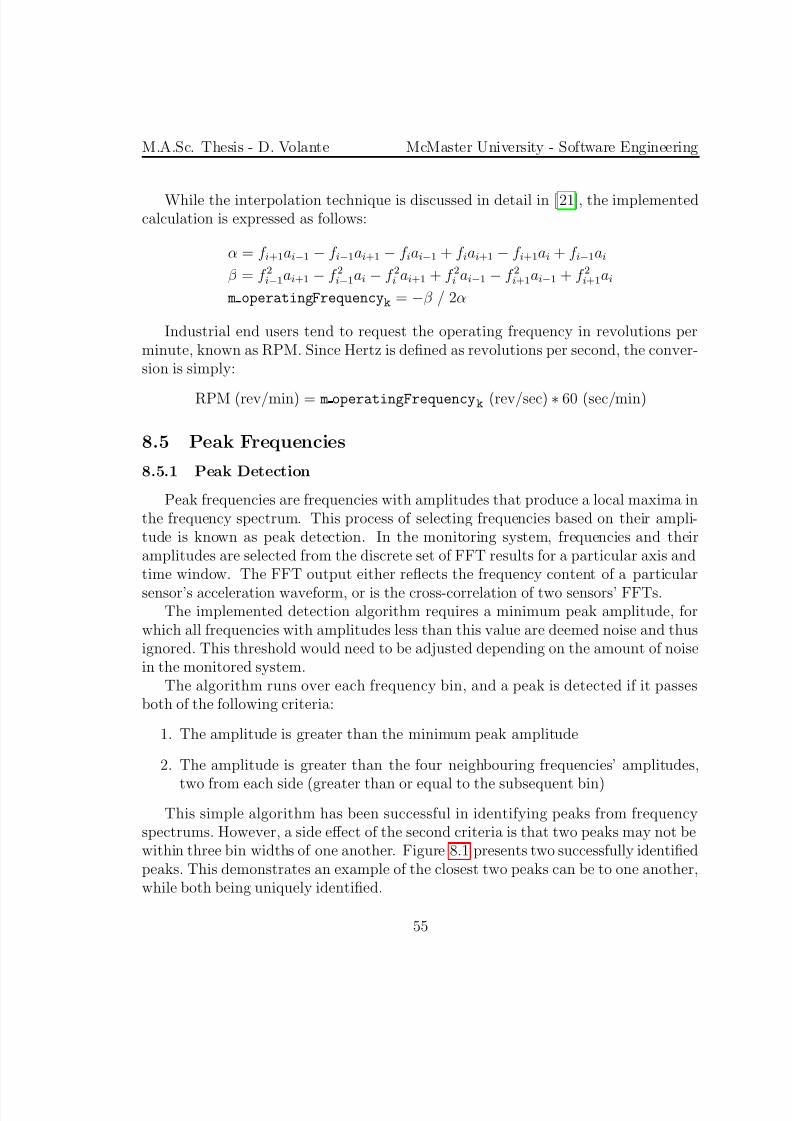
the use of multiple sensor. The detection system cross-correlates eight sets of sensordata with one another and converts the results into the frequency domain. Peakfrequencies are then detected, which reveal what frequencies are shared amongst thesensors and at what strengths. Any identified peak frequencies not present in a healthymachine are then further examined, as they are likely to be the source of a fault. Byobserving where the strongest relationships are for a given frequency, it is possible tolocalize the fault on the machine [21].
A beneficial characteristic of the discussed detection system is that it is computa-tionally efficient. No additional filtering is required, as random noise will not correlateamongst the data sets and be filtered out [21]. This quality has extra importance when
being used for continuous condition monitoring, as processing techniques need to beoptimized. The system currently exists as a post-processing tool apart of a largervibration analysis system. The corresponding paper promoted the expansion of thedetection system for continuous real time monitoring, as well providing it with thefault knowledge of an expert system.
M.A.Sc. Thesis - D. Volante McMaster University - Software Engineering
3 FFT Amplitude Computation
3.1 Overview
The fast Fourier transform (FFT) is a technique used to convert time domainwaveform data into the corresponding frequency content. It is useful when examiningperiodic signals, like the ones produced from the vibrating screens. However due tothe nature of the FFT computation, the result is a discrete set of frequencies andamplitudes. Ultimately, contained frequency content is assigned to the closest FFTfrequency bin. While this reduces the accuracy of measurable frequencies, it alsocreates error in the bin’s amplitude. The further away a frequency is to its respective
bin frequency, the less its contributed amplitude is represented. This form of erroris commonly referred to as FFT leakage, since portions of the lost contribution arerepresented in the amplitudes of neighbouring bins. Since the FFT is to be utilizedin the condition monitoring system, this topic will be further examined.
3.2 Numerical Example
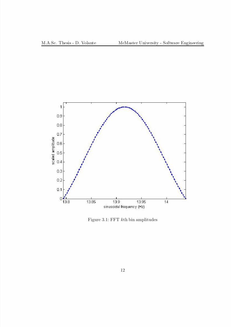
To demonstrate the effect of FFT leakage a numerical experiment was performed.The amplitude of the frequency corresponding to the kth bin was observed for variousinput sinusoidal waves. A wave with frequency of the k-1 bin was first created and
then passed into an FFT. As expected, the amplitude of the kth bin remained at zero,since the frequency matches up with the k-1 bin frequency. The input sinusoidal’sfrequency was slightly incremented and the kth bin amplitude was examined. Thisrepeated until the amplitude of the kth bin returned to zero, as the sinusoidal’sfrequency matched up with the k+1 bin. Figure 3.1 plots the amplitude of the FFT’skth bin output for the range of input frequencies.
It can be seen that the maximum expressed amplitude occurs when the inputfrequency is equivalent to the kth bin frequency. The further away the input frequencyis from this point, the less its amplitude is expressed in the FFT output.
M.A.Sc. Thesis - D. Volante McMaster University - Software Engineering
3.3 Theoretical ModelTo understand the effect of the FFT leakage, the computation of the discrete
Fourier transform is reviewed. The kth bin will be examined, assuming the frequencyof the input sinusoidal is within that bin. The sinusoidal can be expressed as,
x(n) = cos(ωon)
=1
2(eiωon + e−iωon)
Computing the bin amplitude,
X k =N −1
n=0
x(n)e−inkωs
=N −1
n=0
1
2(eiωon + e−iωon)e−inkωs
=1
2
N −1
n=0
(eiωone−inkωs + e−iωone−inkωs)
Ignoring the left hand plane due to symmetry, and simplifying,
M.A.Sc. Thesis - D. Volante McMaster University - Software Engineering
The summation can be expressed,
X k =1
2(
1 − aN
1 − a)
Where,
a = e−i(kωs−ωo)
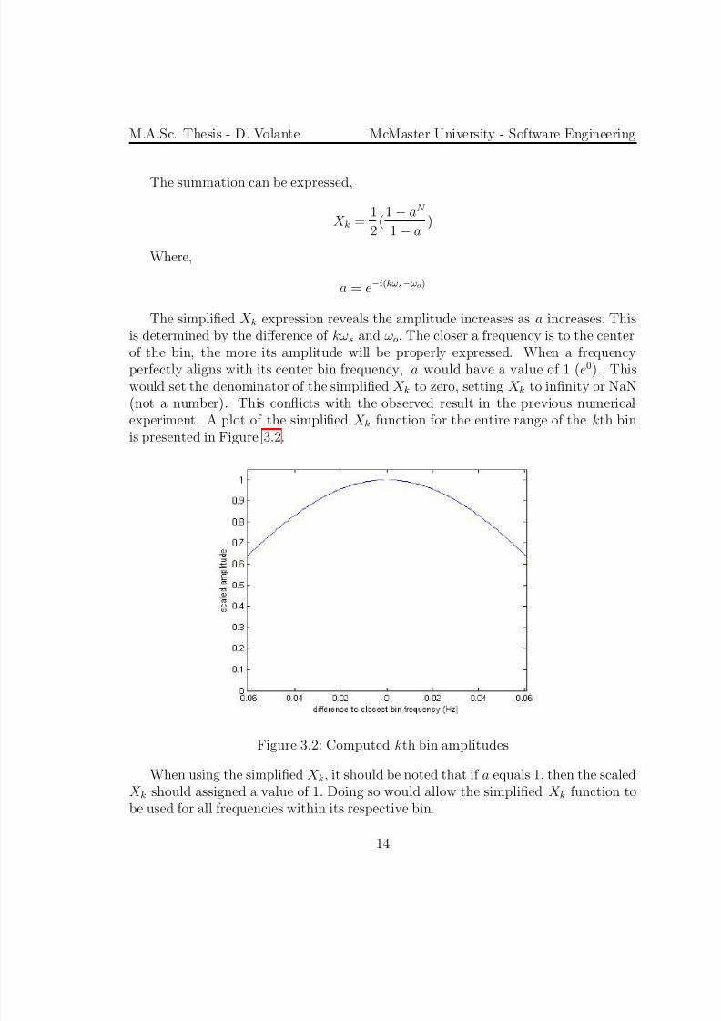
The simplified X k expression reveals the amplitude increases as a increases. Thisis determined by the difference of kωs and ωo. The closer a frequency is to the center
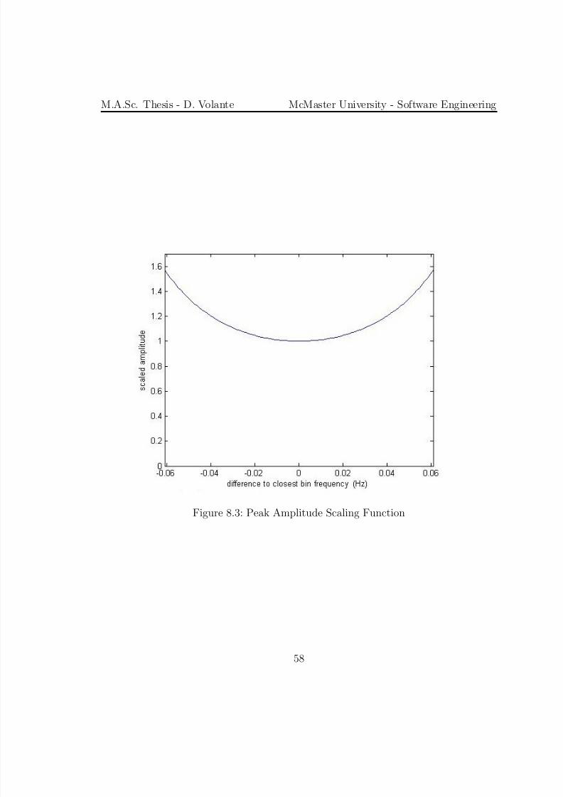
of the bin, the more its amplitude will be properly expressed. When a frequencyperfectly aligns with its center bin frequency, a would have a value of 1 (e0). Thiswould set the denominator of the simplified X k to zero, setting X k to infinity or NaN(not a number). This conflicts with the observed result in the previous numericalexperiment. A plot of the simplified X k function for the entire range of the kth binis presented in Figure 3.2.
Figure 3.2: Computed kth bin amplitudes
When using the simplified X k, it should be noted that if a equals 1, then the scaledX k should assigned a value of 1. Doing so would allow the simplified X k function tobe used for all frequencies within its respective bin.
M.A.Sc. Thesis - D. Volante McMaster University - Software Engineering
4 System Overview
4.1 High Level Overview
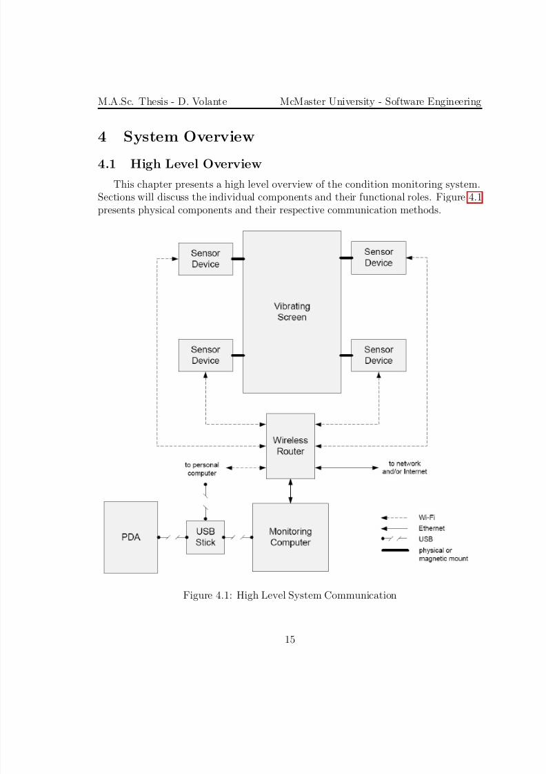
This chapter presents a high level overview of the condition monitoring system.Sections will discuss the individual components and their functional roles. Figure 4.1presents physical components and their respective communication methods.
M.A.Sc. Thesis - D. Volante McMaster University - Software Engineering
4.2 Vibrating ScreensThe vibrating screen is the monitored plant in the system. These machines screen
aggregates through their high rotational accelerations and are able to sort dozens of tonnes of material per hour. Various kinds of vibrating screens exist, operating ineither circular, elliptical or linear motions nearing 1000 RPM.
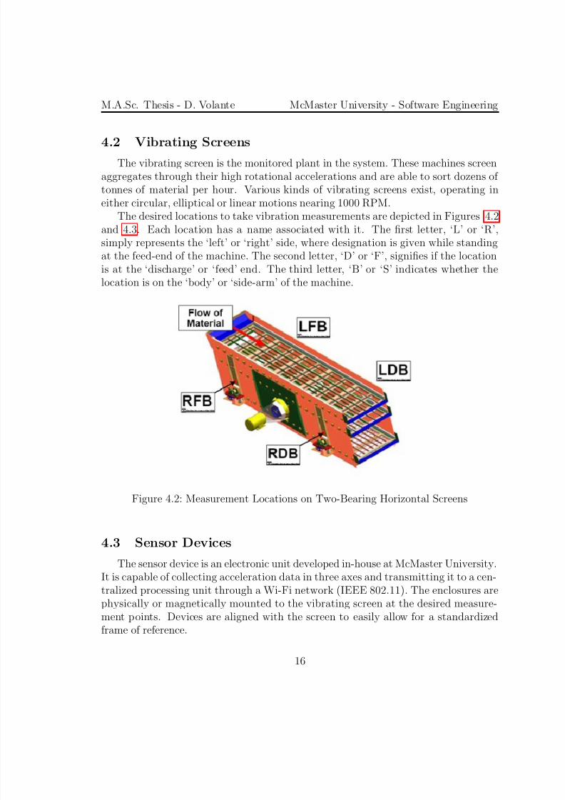
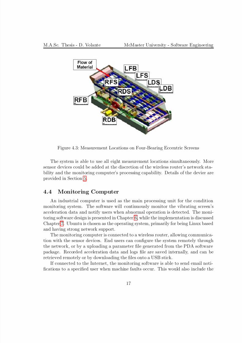
The desired locations to take vibration measurements are depicted in Figures 4.2and 4.3. Each location has a name associated with it. The first letter, ‘L’ or ‘R’,simply represents the ‘left’ or ‘right’ side, where designation is given while standingat the feed-end of the machine. The second letter, ‘D’ or ‘F’, signifies if the locationis at the ‘discharge’ or ‘feed’ end. The third letter, ‘B’ or ‘S’ indicates whether the
location is on the ‘body’ or ‘side-arm’ of the machine.
Figure 4.2: Measurement Locations on Two-Bearing Horizontal Screens
4.3 Sensor Devices
The sensor device is an electronic unit developed in-house at McMaster University.It is capable of collecting acceleration data in three axes and transmitting it to a cen-tralized processing unit through a Wi-Fi network (IEEE 802.11). The enclosures arephysically or magnetically mounted to the vibrating screen at the desired measure-ment points. Devices are aligned with the screen to easily allow for a standardizedframe of reference.
M.A.Sc. Thesis - D. Volante McMaster University - Software Engineering
Figure 4.3: Measurement Locations on Four-Bearing Eccentric Screens
The system is able to use all eight measurement locations simultaneously. Moresensor devices could be added at the discretion of the wireless router’s network sta-bility and the monitoring computer’s processing capability. Details of the device are
provided in Section 5.
4.4 Monitoring Computer
An industrial computer is used as the main processing unit for the conditionmonitoring system. The software will continuously monitor the vibrating screen’sacceleration data and notify users when abnormal operation is detected. The moni-toring software design is presented in Chapter 6, while the implementation is discussedChapter 7. Ubuntu is chosen as the operating system, primarily for being Linux basedand having strong network support.
The monitoring computer is connected to a wireless router, allowing communica-
tion with the sensor devices. End users can configure the system remotely throughthe network, or by a uploading a parameter file generated from the PDA softwarepackage. Recorded acceleration data and logs file are saved internally, and can beretrieved remotely or by downloading the files onto a USB stick.
If connected to the Internet, the monitoring software is able to send email noti-fications to a specified user when machine faults occur. This would also include the
M.A.Sc. Thesis - D. Volante McMaster University - Software Engineering
log file of the trigger event. At the end of a monitoring session, the log file can alsobe emailed so that all triggered fault conditions within the session are known.
4.5 Wireless Router
A standard wireless router is used to support the Wi-Fi network, connecting themonitoring computer to the sensor devices and possibly other networks. Its networkcapacity should exceed the requirements from the set of sensor devices and otherintended wireless access. Section 5.5.2 discusses transmission rates of the implementedsensor devices.
4.6 PDA
Technicians installing and configuring the condition monitoring system have accessto a military grade personal digital assistant (PDA). This unit is a key component in arelated project, the Vibration Analysis Tool [21]. A software package was created forthe PDA so users can select the desired system parameters from a graphical interfaceand download them on to a USB stick. Users can then upload the file to the monitoringcomputer, where it is utilized by the monitoring software.
Due to the dust emitting from the vibrating screens, it is undesirable to use con-ventional electronic devices in the environment. The PDA’s sealed touch screen and
external buttons allows users to interface with the monitoring system while in harshconditions.
4.7 USB Stick
As mentioned, it is possible to specify and download the system parameters ontoa USB stick using the PDA device, so that it can be uploaded into the monitoringcomputer. It is also possible to insert the USB stick into the monitoring computerto download the recorded acceleration data and log files produced by the monitoringsoftware.
M.A.Sc. Thesis - D. Volante McMaster University - Software Engineering
5 Sensor Devices
5.1 Overview
The sensor devices are the data acquisition units of the condition monitoringsystem. Mounted at specified points on the vibrating screen, they are able to collectacceleration data and transmit it to a centralized processing unit. The devices wereinitially developed for a maintenance and troubleshooting tool for vibrating screens.The original device will be briefly discussed, followed by the modifications made toincorporate it into the current monitoring project.
5.2 Existing Devices
The sensor devices were originally used in the Vibration Analysis Tool as the dataacquisition units. The device’s software and hardware were developed at McMasterUniversity; developmental details are provided in its corresponding paper [21]. Thedevices are equipped with an accelerometer, allowing them to measure accelerationsin three axes up to ±10 g, where 1 g is equivalent to 9.81 m/s2. A PIC microprocessorsamples the accelerometer at 500 Hz, converting the analog signal into its digital 12 bitrepresentation. The microprocessor then relays the data to the Bluetooth transceiverusing RS-232, a point-to-point protocol. Bluetooth wirelessly transmits the data to a
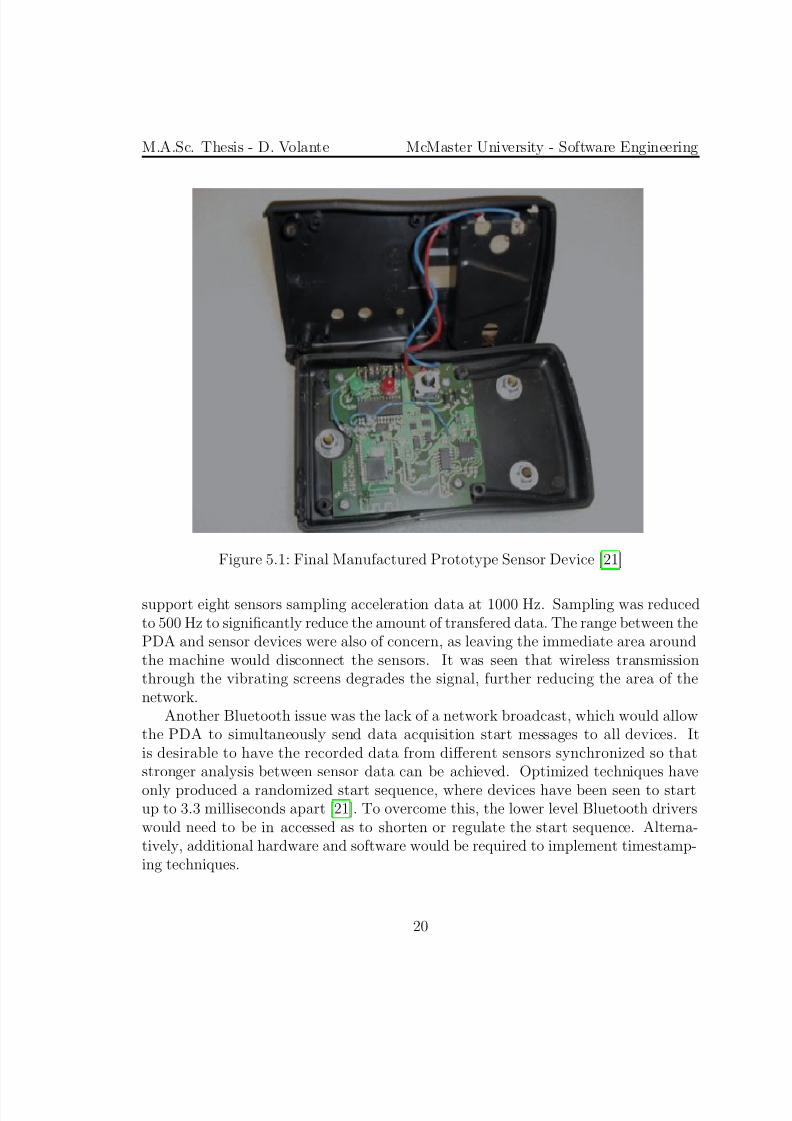
PDA, where centralized analysis takes place.A requirement of the original sensor device was that it must transmit data wire-lessly. Devices are magnetically mounted on to vibrating screens for temporary analy-sis, and then removed when sufficient data was acquired. Wiring would only lengthenthe entire maintenance procedure. Also, with the PDA being held by technicians, itis undesirable and against safety regulations to tether the unit to a vibrating screen.As a result of being completely wireless, two AA batteries are used power the device.Figure 5.1 presents the final manufactured prototype sensor device with its enclosureopened.
While the original sensor device was successfully implemented and is still currentlyin use, it has a few undesired characteristics. These issues arose from the choice of
Bluetooth as the wireless technology. A Bluetooth network (piconet) can only supporteight devices, including the master. Using the PDA with eight sensor devices wouldrequire two Bluetooth networks to sustain the system. The PDA had an internalBluetooth transceiver, and was equipped with and an additional external one as wellto compensate.
The transmission rates of the Bluetooth system were not sufficient enough to
M.A.Sc. Thesis - D. Volante McMaster University - Software Engineering
Figure 5.1: Final Manufactured Prototype Sensor Device [21]
support eight sensors sampling acceleration data at 1000 Hz. Sampling was reducedto 500 Hz to significantly reduce the amount of transfered data. The range between thePDA and sensor devices were also of concern, as leaving the immediate area aroundthe machine would disconnect the sensors. It was seen that wireless transmissionthrough the vibrating screens degrades the signal, further reducing the area of thenetwork.
Another Bluetooth issue was the lack of a network broadcast, which would allowthe PDA to simultaneously send data acquisition start messages to all devices. Itis desirable to have the recorded data from different sensors synchronized so thatstronger analysis between sensor data can be achieved. Optimized techniques have
only produced a randomized start sequence, where devices have been seen to startup to 3.3 milliseconds apart [21]. To overcome this, the lower level Bluetooth driverswould need to be in accessed as to shorten or regulate the start sequence. Alterna-tively, additional hardware and software would be required to implement timestamp-ing techniques.
M.A.Sc. Thesis - D. Volante McMaster University - Software Engineering
5.3 Requirements5.3.1 Technical Requirements
The existing sensor devices and devices used in the condition monitoring systemhave the same technical requirements, as presented below:
• at least eight sensor devices are to be supported by the system
• g-force accelerations are to be monitored in three axes
• g-forces are to be monitored up to ±10 g, where 1 g is equivalent to 9.81 m/s2
• frequency spectrums from at least 0.5 Hz to 249.5 Hz are to be examined
5.3.2 Transmission Requirements
As a result of the technical requirements, a minimum transmission rate can bedetermined. For analysis, eight sensors sampling at 500 Hz will produce the minimumamount of required data. The microprocessor samples three axis of acceleration data,using 12 bit analog to digital conversion. For one device, the transmission rate in bitsper second (bps) is:
For eight sensors and with no communication overhead, the rate is:
System Rate = 18, 000 (bps/device) ∗ 8 (devices)
= 144, 000 bps
This produces a minimum transmission rate that must be exceeded to support thesensor network. Networks that marginally exceed this rate are likely to be unstable,as systems should allow ample capacity for communication overhead. This threshold
is to be used to dismiss communication technologies that are too slow to meet thebare requirements.
Another requirement placed on the communication system is that it must allow thebroadcast of messages. These messages can be received by all devices simultaneously,allowing synchronized device actions to be performed.
M.A.Sc. Thesis - D. Volante McMaster University - Software Engineering
5.4 Upgrade AlternativesIn order to satisfy network requirements and further improve transmission rates
and distance, new means of device communications were investigated. The new tech-nology had to allow messages to be broadcast, and support a network for at least eightdevices and a centralized processing unit. Two main network types were examined:wired and wireless.
5.4.1 Wired Communication
Unlike the original sensor devices, the condition monitoring system does not re-
quire the devices to be wireless. It is intended that the devices are permanentlyinstalled on to a vibrating screen and so wires could be used for power or communi-cation. While wired networks can be expensive to install on vibrating screens, theyallow messages to be broadcast. Since the existing microprocessors are communicat-ing with Bluetooth using RS-232, a multi-point variant, RS-485, was first considered.Modules can be purchased or built to convert the RS-232 to RS-485, and vise-versa.
RS-485, also known as EIA-485, is an electrical standard in defining a multi-pointcommunication network. A maximum of 32 devices can be connected to a singlenetwork. RS-485 utilizes differential signaling over twisted pair to provide high noiseresistance. Texas Instruments reports that its networks are capable of sending signalsup to 2 Mbps when using 50 meter cabling [31].
Ultimately, RS-485 was not chosen because like Bluetooth, more than one networkis required to support the eight devices. The limiting factor was the transmission rateof the PIC microprocessor. Testing confirmed that asynchronous rates over 115.2 kbpswould result in incorrect data communication [21]. In order to ensure network stabil-ity, RS-485 speeds would need to remain under the designated rate. Accommodatingthe slow speeds requires at least two networks to handle the eight devices. With twonetworks, the difficulty in obtaining synchronized sensor data is greatly increased.Alternative wired methods then were investigated.
I2C, Inter-Integrated Circuit, is a synchronous multi-point standard able to handle128 nodes with standard 7 bit addressing. Developed by NXP, I2C networks with
buffers are reported to have data rates up to 400 kbps at 100 meters [11]. Two bufferswere obtained, a NXP I2C-bus extender and a Texas Instruments dual bidirectionalbus buffer. Both chips were tested with the sensor device to determine the I2C networkperformance.
The NXP I2C-bus extender (P82B715) is a bidirectional buffer with unity voltagegain that can improve the range of an I2C network by increasing cabling impedance.
M.A.Sc. Thesis - D. Volante McMaster University - Software Engineering
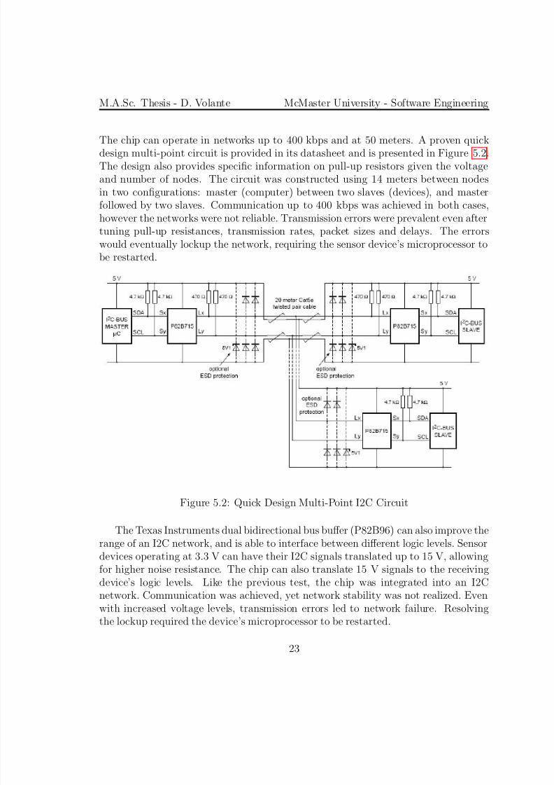
The chip can operate in networks up to 400 kbps and at 50 meters. A proven quickdesign multi-point circuit is provided in its datasheet and is presented in Figure 5.2.The design also provides specific information on pull-up resistors given the voltageand number of nodes. The circuit was constructed using 14 meters between nodesin two configurations: master (computer) between two slaves (devices), and masterfollowed by two slaves. Communication up to 400 kbps was achieved in both cases,however the networks were not reliable. Transmission errors were prevalent even aftertuning pull-up resistances, transmission rates, packet sizes and delays. The errorswould eventually lockup the network, requiring the sensor device’s microprocessor tobe restarted.
Figure 5.2: Quick Design Multi-Point I2C Circuit
The Texas Instruments dual bidirectional bus buffer (P82B96) can also improve therange of an I2C network, and is able to interface between different logic levels. Sensordevices operating at 3.3 V can have their I2C signals translated up to 15 V, allowingfor higher noise resistance. The chip can also translate 15 V signals to the receivingdevice’s logic levels. Like the previous test, the chip was integrated into an I2Cnetwork. Communication was achieved, yet network stability was not realized. Evenwith increased voltage levels, transmission errors led to network failure. Resolvingthe lockup required the device’s microprocessor to be restarted.
M.A.Sc. Thesis - D. Volante McMaster University - Software Engineering
To compensate for the I2C network lockup, additional circuitry and software wouldbe required. The network would need to be continuously monitored to ensure thatnodes do not hold communication lines at logic low. Nodes doing so restrict anyother device from being able transmit data, rendering the network unusable. Anautomated routine would be required to restart the devices’ microprocessors, andnotify the network master in such a failure event. However, any communicationinterruption is undesirable as it is not be possible to perform condition monitoringwithout sensor data. It was concluded that due to poor reliability and transmissionrate of the microprocessor, using a wired network would be unadvantageous.
5.4.2 Wireless CommunicationWhen the existing sensor device was developed, the alternatives to Bluetooth were
ZigBee and Wi-Fi. ZigBee was ruled out for being a niche product, as componentswere difficult to obtain. Wi-Fi was not originally chosen because of its power require-ments. While it had high data rates and ranges, the power draw was too much fora wireless device [21]. Technology has advanced over the last few years and new Wi-Fi products are available. As these Wi-Fi transceivers now have comparable powerconsumption to Bluetooth, they are reexamined as a wireless technology.
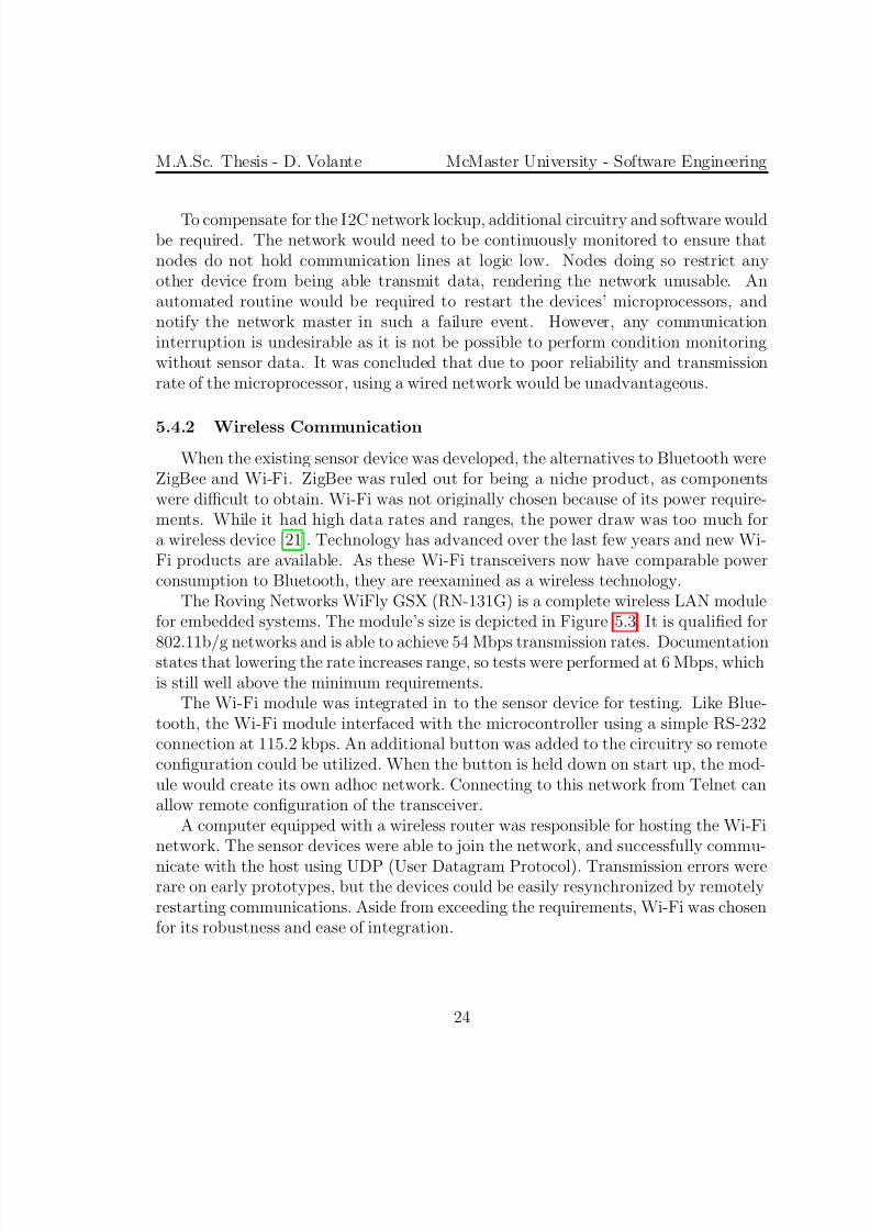
The Roving Networks WiFly GSX (RN-131G) is a complete wireless LAN modulefor embedded systems. The module’s size is depicted in Figure 5.3. It is qualified for
802.11b/g networks and is able to achieve 54 Mbps transmission rates. Documentationstates that lowering the rate increases range, so tests were performed at 6 Mbps, whichis still well above the minimum requirements.
The Wi-Fi module was integrated in to the sensor device for testing. Like Blue-tooth, the Wi-Fi module interfaced with the microcontroller using a simple RS-232connection at 115.2 kbps. An additional button was added to the circuitry so remoteconfiguration could be utilized. When the button is held down on start up, the mod-ule would create its own adhoc network. Connecting to this network from Telnet canallow remote configuration of the transceiver.
A computer equipped with a wireless router was responsible for hosting the Wi-Finetwork. The sensor devices were able to join the network, and successfully commu-
nicate with the host using UDP (User Datagram Protocol). Transmission errors wererare on early prototypes, but the devices could be easily resynchronized by remotelyrestarting communications. Aside from exceeding the requirements, Wi-Fi was chosenfor its robustness and ease of integration.
M.A.Sc. Thesis - D. Volante McMaster University - Software Engineering
Figure 5.3: Roving Networks WiFly GSX [16]
5.5 Communication Upgrade
Wi-Fi was chosen as the new communication technology, and so the sensor deviceswere fully integrated with the WiFly GSX modules. The internal functionality of thedevice remains the same as the existing one, however the communication protocol hasbeen modified. As a result, the revised protocol will be discussed.
5.5.1 Control Protocol
The same control characters from the existing device are used, along with anadditional two. The host computer now initiates the wireless communication by
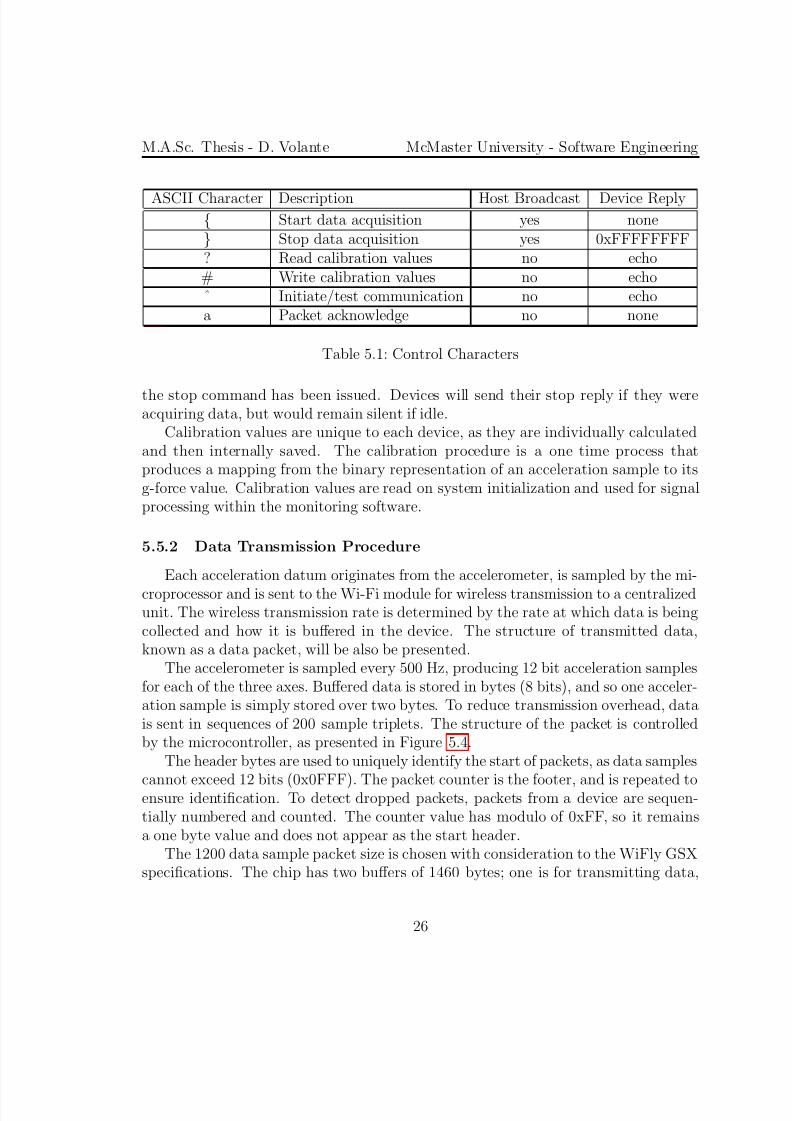
requesting an echoed test character. Acknowledgments are also now used after eachreceived packet, as to be aware of data delivery. While brief descriptions are providedin Table 5.1 and in the following paragraph, full functional details are provided inoriginal paper [21].
The start command is simultaneously sent to all devices, commencing their dataacquisition. Packets of sampled acceleration data are sent to a centralized unit until
M.A.Sc. Thesis - D. Volante McMaster University - Software Engineering
ASCII Character Description Host Broadcast Device Reply{ Start data acquisition yes none} Stop data acquisition yes 0xFFFFFFFF? Read calibration values no echo# Write calibration values no echoˆ Initiate/test communication no echoa Packet acknowledge no none
Table 5.1: Control Characters
the stop command has been issued. Devices will send their stop reply if they wereacquiring data, but would remain silent if idle.
Calibration values are unique to each device, as they are individually calculatedand then internally saved. The calibration procedure is a one time process thatproduces a mapping from the binary representation of an acceleration sample to itsg-force value. Calibration values are read on system initialization and used for signalprocessing within the monitoring software.
5.5.2 Data Transmission Procedure
Each acceleration datum originates from the accelerometer, is sampled by the mi-
croprocessor and is sent to the Wi-Fi module for wireless transmission to a centralizedunit. The wireless transmission rate is determined by the rate at which data is beingcollected and how it is buffered in the device. The structure of transmitted data,known as a data packet, will be also be presented.
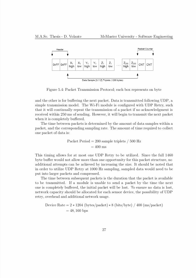
The accelerometer is sampled every 500 Hz, producing 12 bit acceleration samplesfor each of the three axes. Buffered data is stored in bytes (8 bits), and so one acceler-ation sample is simply stored over two bytes. To reduce transmission overhead, datais sent in sequences of 200 sample triplets. The structure of the packet is controlledby the microcontroller, as presented in Figure 5.4.
The header bytes are used to uniquely identify the start of packets, as data samples
cannot exceed 12 bits (0x0FFF). The packet counter is the footer, and is repeated toensure identification. To detect dropped packets, packets from a device are sequen-tially numbered and counted. The counter value has modulo of 0xFF, so it remainsa one byte value and does not appear as the start header.
The 1200 data sample packet size is chosen with consideration to the WiFly GSXspecifications. The chip has two buffers of 1460 bytes; one is for transmitting data,
M.A.Sc. Thesis - D. Volante McMaster University - Software Engineering
Figure 5.4: Packet Transmission Protocol; each box represents on byte
and the other is for buffering the next packet. Data is transmitted following UDP, asimple transmission model. The Wi-Fi module is configured with UDP Retry, suchthat it will continually repeat the transmission of a packet if no acknowledgment isreceived within 250 ms of sending. However, it will begin to transmit the next packetwhen it is completely buffered.
The time between packets is determined by the amount of data samples within apacket, and the corresponding sampling rate. The amount of time required to collectone packet of data is:
Packet Period = 200 sample triplets / 500 Hz
= 400 ms
This timing allows for at most one UDP Retry to be utilized. Since the full 1460byte buffer would not allow more than one opportunity for this packet structure, noadditional attempts can be achieved by increasing the size. It should be noted thatin order to utilize UDP Retry at 1000 Hz sampling, sampled data would need to beput into larger packets and compressed.
The time between subsequent packets is the duration that the packet is availableto be transmitted. If a module is unable to send a packet by the time the nextone is completely buffered, the initial packet will be lost. To ensure no data is lost,network capacity should be allocated for each sensor device, the possibility of UDPretry, overhead and additional network usage.
M.A.Sc. Thesis - D. Volante McMaster University - Software Engineering
For eight sensors and with no communication overhead, the rate is:
System Rate = 48, 160 (bps/device) ∗ 8 (devices)
= 385, 280 bps
The implemented sensor devices operate at 6 Mbps, allowing for over 1500% of communication overhead. With the excessive capacity, each device will have amplenetwork opportunity to transmit its packets.
M.A.Sc. Thesis - D. Volante McMaster University - Software Engineering
6 Monitoring Software Design
6.1 Design Model
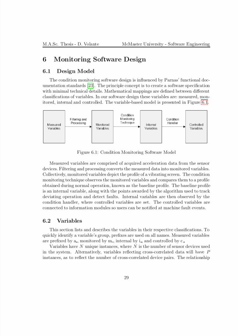
The condition monitoring software design is influenced by Parnas’ functional doc-umentation standards [23]. The principle concept is to create a software specificationwith minimal technical details. Mathematical mappings are defined between differentclassifications of variables. In our software design these variables are: measured, mon-itored, internal and controlled. The variable-based model is presented in Figure 6.1.
Figure 6.1: Condition Monitoring Software Model
Measured variables are comprised of acquired acceleration data from the sensordevices. Filtering and processing converts the measured data into monitored variables.
Collectively, monitored variables depict the profile of a vibrating screen. The conditionmonitoring technique observes the monitored variables and compares them to a profileobtained during normal operation, known as the baseline profile. The baseline profileis an internal variable, along with the points awarded by the algorithm used to trackdeviating operation and detect faults. Internal variables are then observed by thecondition handler, where controlled variables are set. The controlled variables areconnected to information modules so users can be notified at machine fault events.
6.2 Variables
This section lists and describes the variables in their respective classifications. To
quickly identify a variable’s group, prefixes are used on all names. Measured variablesare prefixed by a , monitored by m , internal by i , and controlled by c .
Variables have N unique instances, where N is the number of sensor devices usedin the system. Alternatively, variables reflecting cross-correlated data will have P instances, as to reflect the number of cross-correlated device pairs. The relationship
M.A.Sc. Thesis - D. Volante McMaster University - Software Engineering
between N and P is as follows:
P = (N − 1) + (N − 2) + ... + 1
6.2.1 Measured Variables
Measured variables are collected acceleration data from the sensor devices. Thereare N streams of raw data entering the software system. The variable has an equiva-lent definition for all three axes, as presented in Table 6.1.
Name Type Description
a accDk,k=x,y,z integer raw acceleration datum
Table 6.1: Measured Variables
The interval between subsequent data from the same sensor and axis is inverselyrelated to the sensor’s sampling rate. Acceleration data is to be sampled at 500 Hz,so the interval between subsequent data is 2 milliseconds.
6.2.2 Monitored Variables
The machine’s condition is observed through the monitored variables. They arethe result of filtering and processing the measured variables. Their implemented defi-nitions are presented Chapter 8. Each of the N sensor devices has a profile depictingthe machine’s operation. The device profile type is presented in Table 6.2.
Name Type Description
m mainGForce real main g-force m averageGForcek,k=x,y,z real average g-force
m operatingFrequencyk,k=x,y real operating frequency in Hz
m peakListk,k=x,y,z peakList list of peak frequencies
Table 6.2: Monitored Variables in deviceProfile
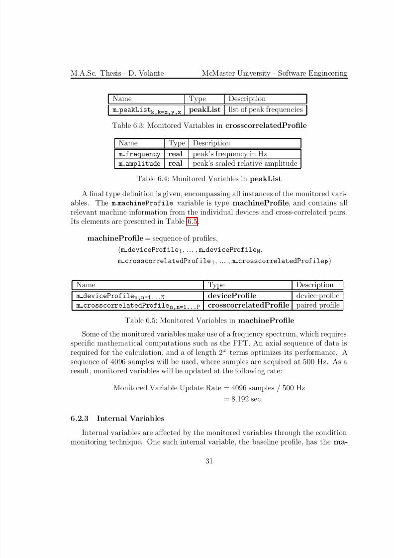
Regarding cross-correlated data, only the peak frequencies are monitored. Thereare P instances of a cross-correlated profile. Its type is presented in Table 6.3.
The definition of the peakList type is given below. It is followed by the elementsused in its construction, as presented in Table 6.4.
peakList = sequence of pairs: m frequency, m amplitude
M.A.Sc. Thesis - D. Volante McMaster University - Software Engineering
Name Type Description m peakListk,k=x,y,z peakList list of peak frequencies
Table 6.3: Monitored Variables in crosscorrelatedProfile
Name Type Description
m frequency real peak’s frequency in Hz m amplitude real peak’s scaled relative amplitude
Table 6.4: Monitored Variables in peakList
A final type definition is given, encompassing all instances of the monitored vari-ables. The m machineProfile variable is type machineProfile, and contains allrelevant machine information from the individual devices and cross-correlated pairs.Its elements are presented in Table 6.5.
machineProfile = sequence of profiles,
( m deviceProfile1, ... , m deviceProfileN,
m crosscorrelatedProfile1, ... , m crosscorrelatedProfileP)
Name Type Description
m deviceProfilen,n=1...N deviceProfile device profile m crosscorrelatedProfilen,n=1...P crosscorrelatedProfile paired profile
Table 6.5: Monitored Variables in machineProfile
Some of the monitored variables make use of a frequency spectrum, which requiresspecific mathematical computations such as the FFT. An axial sequence of data isrequired for the calculation, and a of length 2x terms optimizes its performance. Asequence of 4096 samples will be used, where samples are acquired at 500 Hz. As aresult, monitored variables will be updated at the following rate:
Internal variables are affected by the monitored variables through the conditionmonitoring technique. One such internal variable, the baseline profile, has the ma-
M.A.Sc. Thesis - D. Volante McMaster University - Software Engineering
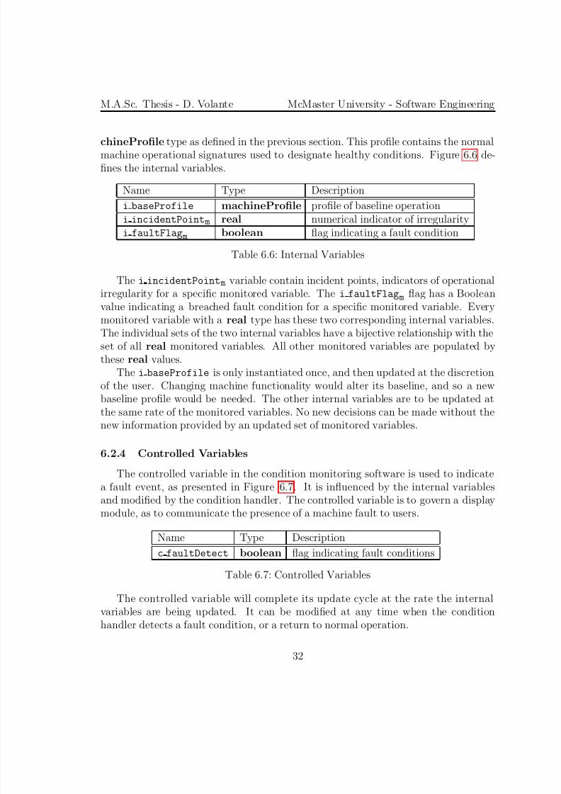
chineProfile type as defined in the previous section. This profile contains the normalmachine operational signatures used to designate healthy conditions. Figure 6.6 de-fines the internal variables.
Name Type Description
i baseProfile machineProfile profile of baseline operationi incidentPoint m real numerical indicator of irregularityi faultFlag m boolean flag indicating a fault condition
Table 6.6: Internal Variables
The i incidentPoint m variable contain incident points, indicators of operationalirregularity for a specific monitored variable. The i faultFlag m flag has a Booleanvalue indicating a breached fault condition for a specific monitored variable. Everymonitored variable with a real type has these two corresponding internal variables.The individual sets of the two internal variables have a bijective relationship with theset of all real monitored variables. All other monitored variables are populated bythese real values.
The i baseProfile is only instantiated once, and then updated at the discretionof the user. Changing machine functionality would alter its baseline, and so a newbaseline profile would be needed. The other internal variables are to be updated at
the same rate of the monitored variables. No new decisions can be made without thenew information provided by an updated set of monitored variables.
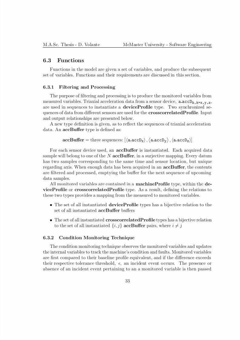
6.2.4 Controlled Variables
The controlled variable in the condition monitoring software is used to indicatea fault event, as presented in Figure 6.7. It is influenced by the internal variablesand modified by the condition handler. The controlled variable is to govern a displaymodule, as to communicate the presence of a machine fault to users.
Name Type Description
c faultDetect boolean flag indicating fault conditionsTable 6.7: Controlled Variables
The controlled variable will complete its update cycle at the rate the internalvariables are being updated. It can be modified at any time when the conditionhandler detects a fault condition, or a return to normal operation.
M.A.Sc. Thesis - D. Volante McMaster University - Software Engineering
6.3 FunctionsFunctions in the model are given a set of variables, and produce the subsequent
set of variables. Functions and their requirements are discussed in this section.
6.3.1 Filtering and Processing
The purpose of filtering and processing is to produce the monitored variables frommeasured variables. Triaxial acceleration data from a sensor device, a accDk,k=x,y,z,are used in sequences to instantiate a deviceProfile type. Two synchronized se-quences of data from different sensors are used for the crosscorrelatedProfile. Input
and output relationships are presented below.A new type definition is given, as to reflect the sequences of triaxial acceleration
data. An accBuffer type is defined as:
accBuffer = three sequences: [a accDx ,
a accDy
, a accDz]
For each sensor device used, an accBuffer is instantiated. Each acquired datasample will belong to one of the N accBuffer, in a surjective mapping. Every datumhas two samples corresponding to the same time and sensor location, but uniqueregarding axis. When enough data has been acquired in an accBuffer, the contentsare filtered and processed, emptying the buffer for the next sequence of upcoming
data samples.All monitored variables are contained in a machineProfile type, within the de-
viceProfile or crosscorrelatedProfile type. As a result, defining the relations tothese two types provides a mapping from the measured to monitored variables.
• The set of all instantiated deviceProfile types has a bijective relation to theset of all instantiated accBuffer buffers
• The set of all instantiated crosscorrelatedProfile types has a bijective relationto the set of all instantiated {i, j} accBuffer pairs, where i = j
6.3.2 Condition Monitoring Technique
The condition monitoring technique observes the monitored variables and updatesthe internal variables to track the machine’s condition and faults. Monitored variablesare first compared to their baseline profile equivalent, and if the difference exceedstheir respective tolerance threshold, , an incident event occurs. The presence orabsence of an incident event pertaining to an a monitored variable is then passed
M.A.Sc. Thesis - D. Volante McMaster University - Software Engineering
along to the remainder of the monitoring process. The condition of a monitoredvariable is tracked using the incidents, and is responsible for distinguishing betweenmachine faults and normal operation.
The existence of an incident will be expressed as a Boolean, in the incidentFlag
flag. Each of the monitored variables with a real type are used to check for corre-sponding incidents, as defined below.
For a sensor n [1, N ],
∀m : (m, , , ) ∈ m machineProfile,
(∃mb : (mb, , , ) ∈ i baseProfile,
(|mb − m|/mb ≥ m) ⇔ incidentFlag)
For a sensor n [1, N ], and for an axis k {x,y,z },
∀g : ( , g , , ) ∈ m machineProfile,
(∀gb : ( , gb, , ) ∈ i baseProfile,
(|gb − g|/gb ≥ g) ⇔ incidentFlag)
For a sensor n [1, N ], and for an axis k {x, y},
∀ p : ( , , p , ) ∈ m machineProfile,
(∃ pb : ( , , pb, ) ∈ i baseProfile,
(| pb − p| ≥ p) ⇔ incidentFlag)
For a sensor n [1, N ] or cross-correlated pair p [1, P ], and for an axis k {x,y,z },
∀l : ( , , , l) ∈ m machineProfile, ∀ f, a ∈ l,
(¬∃lb : ( , , , lb) ∈ i baseProfile, ∀ f b, ab ∈ lb,
((|f b − f | < f ) ∧ (|ab − a|/ab < a)) ⇔ incidentFlag)
After the incidentFlag is assigned a Boolean value, the respective modifica-
tions are made to the corresponding i incidentPoint m or i faultFlag m internalvariables. While there are no specific requirements on this process, the set of alli incidentPoint m contains the indicators representing the incident events. The setof all i faultFlag m flags identifies when the algorithm has identified a fault conditionon a specific monitored parameter.
M.A.Sc. Thesis - D. Volante McMaster University - Software Engineering
6.3.3 Condition Handler
The condition handler modifies the controlled variables in response to the internalvariables. The detection of any one fault, corresponding to a particular monitoredvariable, will activate the machine fault flag. The Boolean value of this controlledvariable, c faultDetect, is simply defined as follows.
M.A.Sc. Thesis - D. Volante McMaster University - Software Engineering
7 Monitoring Software Implementation
7.1 Overview
The condition monitoring software is a required subsystem apart of the monitoringproject. The software supports the completion of the thesis objectives, Section 1.2,and follows the framework provided in its design model, Chapter 6. The softwareis implemented in the C programming language and is executed by the system’smonitoring computer.
The program has a command line interface that allows users to initiate the moni-toring process and auxiliary modules. A PDA application has been developed to allow
users to generate a parameter file containing information and settings, which is thenuploaded via USB stick to the monitoring software.
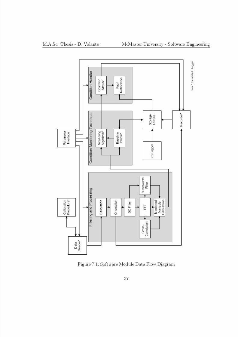
Figure 7.1 presents the main modules that comprise the software, and the corre-sponding data flow between them. Modules will be listed in a module guide, presentedwith their software loops, and have individual details discussed in the following sec-tions.
7.2 Module Guide
This section contains a Module Guide of the software system as defined by Par-
nas [22]. Its purpose is to ensure separation of concerns and assist in future mainte-nance of the modules. Parnas wrote,
It defines the responsibilities of each of the modules by describing thedesign decisions that will be hidden (encapsulated) by that module (itssecrets). [22]
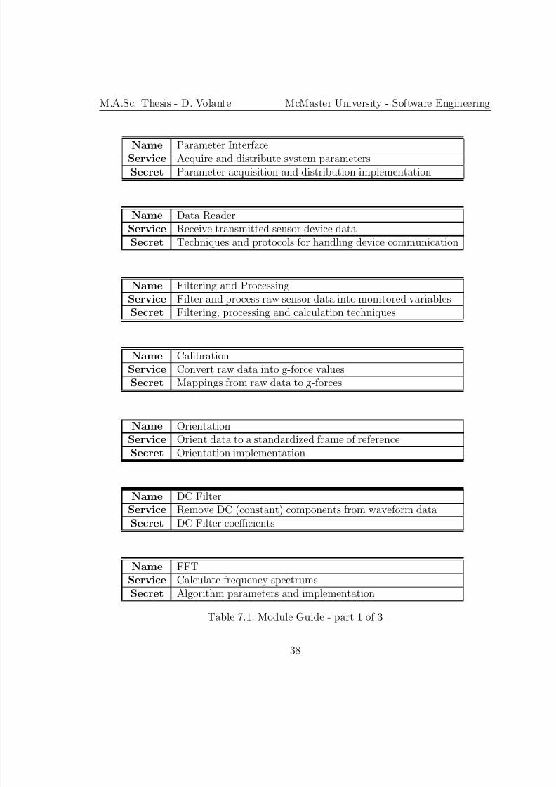
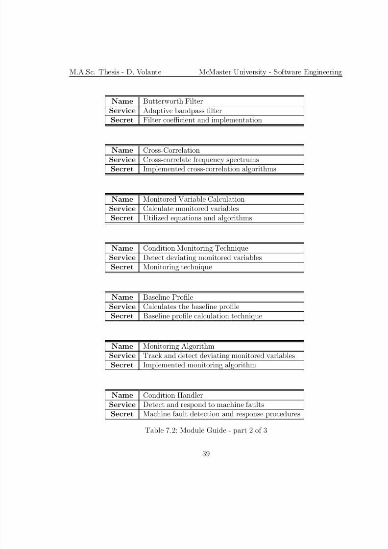
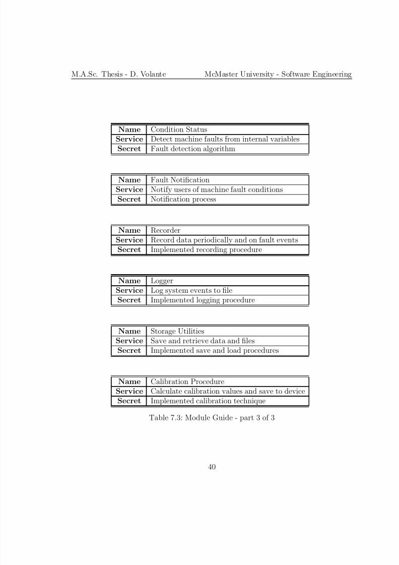
The name, service and secret of each module are presented below. The ModuleGuide spans across Tables 7.1, 7.2 and 7.3.
M.A.Sc. Thesis - D. Volante McMaster University - Software Engineering
Name Parameter InterfaceService Acquire and distribute system parametersSecret Parameter acquisition and distribution implementation
Name Data ReaderService Receive transmitted sensor device dataSecret Techniques and protocols for handling device communication
Name Filtering and ProcessingService Filter and process raw sensor data into monitored variablesSecret Filtering, processing and calculation techniques
Name CalibrationService Convert raw data into g-force valuesSecret Mappings from raw data to g-forces
Name OrientationService Orient data to a standardized frame of referenceSecret Orientation implementation
Name DC FilterService Remove DC (constant) components from waveform dataSecret DC Filter coefficients
Name FFTService Calculate frequency spectrumsSecret Algorithm parameters and implementation
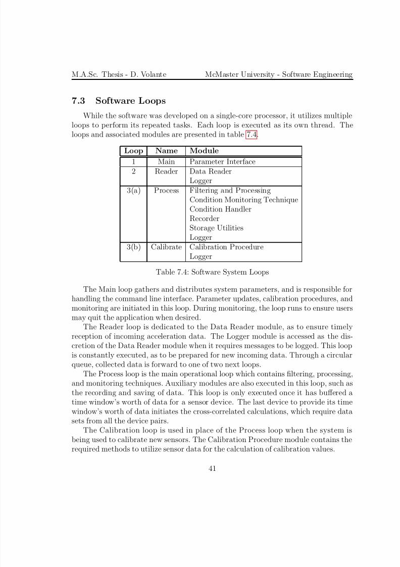
The Main loop gathers and distributes system parameters, and is responsible for
handling the command line interface. Parameter updates, calibration procedures, andmonitoring are initiated in this loop. During monitoring, the loop runs to ensure usersmay quit the application when desired.
The Reader loop is dedicated to the Data Reader module, as to ensure timelyreception of incoming acceleration data. The Logger module is accessed as the dis-cretion of the Data Reader module when it requires messages to be logged. This loopis constantly executed, as to be prepared for new incoming data. Through a circularqueue, collected data is forward to one of two next loops.
The Process loop is the main operational loop which contains filtering, processing,and monitoring techniques. Auxiliary modules are also executed in this loop, such asthe recording and saving of data. This loop is only executed once it has buffered atime window’s worth of data for a sensor device. The last device to provide its timewindow’s worth of data initiates the cross-correlated calculations, which require datasets from all the device pairs.
The Calibration loop is used in place of the Process loop when the system isbeing used to calibrate new sensors. The Calibration Procedure module contains therequired methods to utilize sensor data for the calculation of calibration values.
M.A.Sc. Thesis - D. Volante McMaster University - Software Engineering
7.4 Filtering and ProcessingFiltering and Processing contains the procedures to manipulate raw acceleration
data into meaning information. The result is a collection of monitored variables,specific to individual devices and device pairs. Since the frequency spectrum of thesensor devices’ axes are computed every time window, all monitored variables areupdated at the same rate. This simplifies the continuous monitoring process into themonitoring of discrete time windows. As a result, every module will process data inbuffers corresponding to the amount of acceleration data pertaining to a single timewindow.
Raw acceleration data is introduced into the software by the Data Reader module,
and then stored into circular queues specific to a device and axis (X, Y, Z). TheFiltering and Processing module buffers this data into sized sequences, and thenpasses the data through the various filters and processing techniques.
7.4.1 Calibration
At system initialization, the Calibration module is provided with calibration valuesunique to each sensor device and axis. Since each device stores these values internally,they are acquired by the Data Reader module. Each sensor axis has two calibrationvalues associated with it, mk and bk. This provides a linear mapping from a rawacceleration datum to a g-force value.
y(n) = mkx(n) + bk
The stored calibration values are calculated within the Calibration Procedure mod-ule. Details of this calibration technique are outlined in Section 7.7.6.
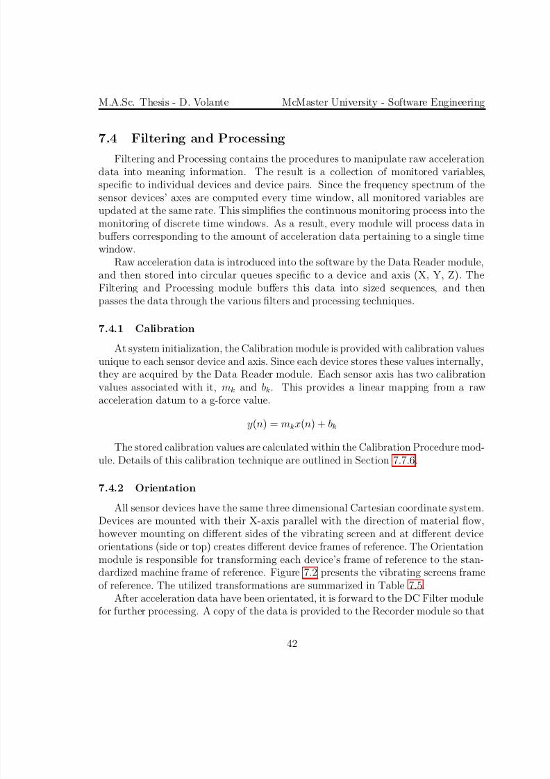
7.4.2 Orientation
All sensor devices have the same three dimensional Cartesian coordinate system.Devices are mounted with their X-axis parallel with the direction of material flow,however mounting on different sides of the vibrating screen and at different device
orientations (side or top) creates different device frames of reference. The Orientationmodule is responsible for transforming each device’s frame of reference to the stan-dardized machine frame of reference. Figure 7.2 presents the vibrating screens frameof reference. The utilized transformations are summarized in Table 7.5.
After acceleration data have been orientated, it is forward to the DC Filter modulefor further processing. A copy of the data is provided to the Recorder module so that
M.A.Sc. Thesis - D. Volante McMaster University - Software Engineering
Figure 7.2: Vibrating Screen - Frame of Reference
Machine Side Device Orientation Transformation
right side or top negate X-axisleft side negate Z-axis
right top flip -Y and Z-axisleft top flip Y and Z-axis
Table 7.5: Sensor Device to Vibrating Screen Frame of Reference
the data can be saved to file when desired. It was decided to record acceleration dataafter minimal processing, while not requiring additional information about the datasequences such as calibration values and device orientations.
7.4.3 DC Filter
The DC Filter module removes constant components from the sensors accelerationdata. The X and Y-axis are subject to gravity, which does not reflect the machineoperation. In order to ignore these constant g-forces, each acceleration datum, withthe previous datums’s original and scaled value, are pass through the following filter.
M.A.Sc. Thesis - D. Volante McMaster University - Software Engineering
The value of R dictates the aggressiveness of the filter, and values between 0.9to 1.0 are typically used. Smaller values accommodate drifting DC components, butsince gravity does not change, a higher value was chosen. The Vibration AnalysisTool found that a relatively high value, R = 0.98, was able to completely removegravity from vibrating screen’s data after a few hundred samples [21]. This value of R is also used in the current implementation.
The more the DC filter is iterated, the more it can better filter out constantcomponents. As a result, the first couple time windows of data are filtered, yet notused in the monitoring process. This allows the construction of the baseline profileand comparison techniques to commence after the filters has completely stabilized.
7.4.4 FFT
The FFT module converts time domain acceleration data into its frequency domainequivalent. The result is a discrete list of frequencies, and corresponding amplitudesdepicting signal contribution or strength. The distance between discrete frequenciesis determined by the sensor sampling rate and size of the input data sequence. It iscommonly referred to as the bin size and in the current implementation it is:
bin size = f (n + 1) − f (n) = (sampling rate) / (data length)
= 500.0 Hz / 4096
= 0.12207 Hz
The usable frequency content is limited to half the sampling rate, known as theNyquist frequency. Content at and above this limit are subject to aliasing, whichcan introduce frequency based errors into the monitoring process. For the currentimplementation, the Nyquist frequency is simply:
Nyquist frequency = (sampling rate) / 2.0
= 500.0 Hz / 2.0
= 250.0 Hz
At the core of this module is the fast Fourier transform (FFT), provided by anopen source library, Fastest Fourier Transform in the West (FFTW). Developed atMIT, this transform is popularized by its speed, portability and usability. At systeminitialization, the input data size is provided to the library where it then creates anoptimized routine for the given length. The FFTW provides complex results, butsince phase information is not required, the absolute magnitude of the complex values
M.A.Sc. Thesis - D. Volante McMaster University - Software Engineering
are taken.The computed frequency spectrum is provided to the Cross-Correlation and Moni-
tored Variable Calculation modules for further processing. The frequency correspond-ing to the largest amplitude, the operating frequency, is provided to the ButterworthFilter module. The Butterworth filter filters around a specific frequency, and so anargument of the maximum function (argmax ) within the FFT module provides it withthis value.
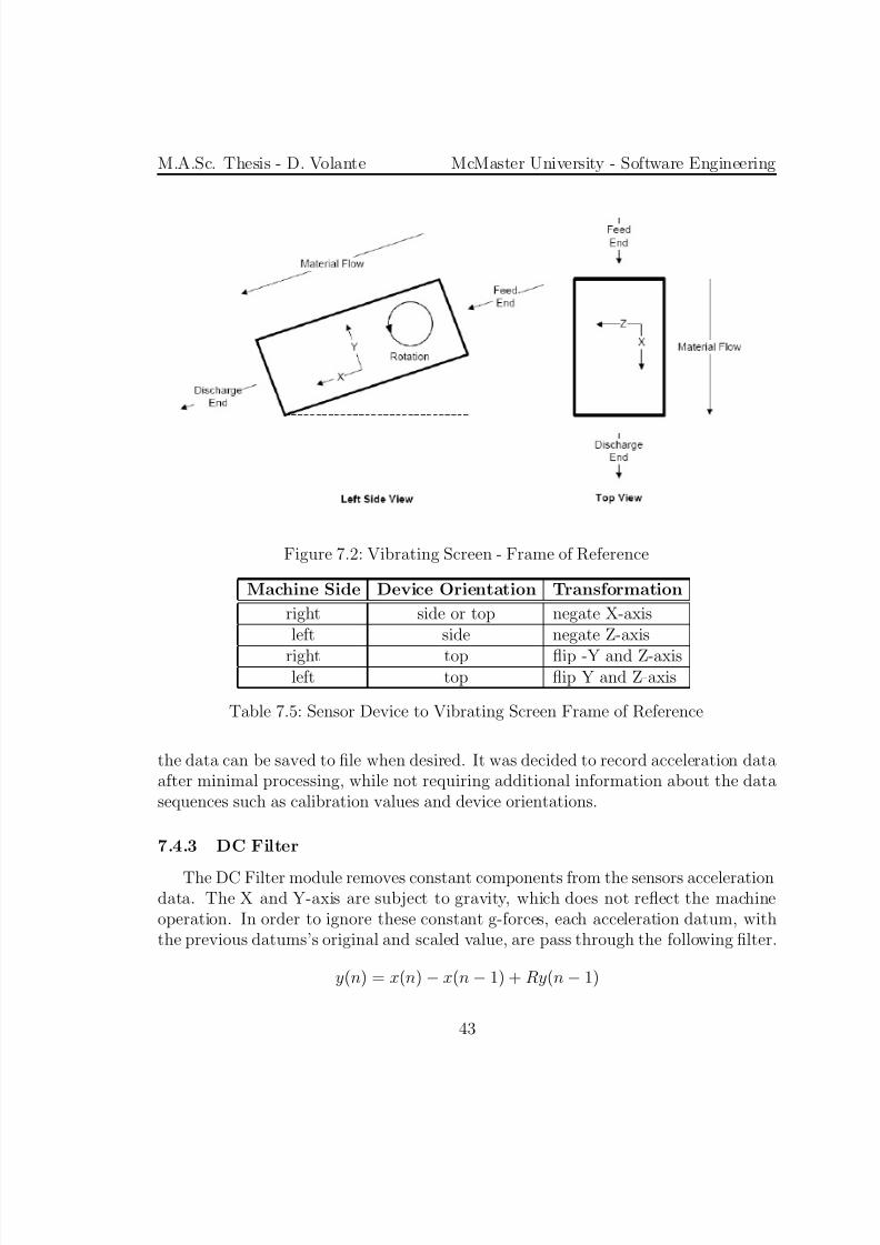
7.4.5 Butterworth Filter
The Butterworth Filter module contains the implemented band-pass filter used to‘smooth’ time domain acceleration data. It is primarily used to remove high-frequencycontent, so that subsequent processing can be carried out without the presence of noise. The filter is centered around the operating frequency, provided by the FFTmodule, and any frequency content outside of the bandwidth is attenuated.
The implemented Butterworth filter follows the design from the Vibration Anal-ysis Tool, where noise was successfully removed from vibrating screens’ accelerationdata [21]. Characteristics of the filter are presented in Table 7.6.
Center Frequency dynamicCenter Frequency Tolerance ±2.0 Hz
Bandwidth ±5.0 HzOrder 4thCoefficients 9
Table 7.6: Butterworth Filter Characteristics
The Butterworth filter utilizes computed coefficients in the filtering process, wherecoefficients are updated when the the center frequency changes. To regulate updates,new coefficients are only calculated when the the center frequency exceeds its toler-ance.
Butterworth filters also require a settling time in order to produce meaningful
results. Filter outputs start at zero and oscillate with increasing amplitudes untilafter a few hundred data points when it stabilizes. To ensure the filter has settledbefore monitoring calculations have begun, the first couple time windows of data arecompletely filtered, and then discarded.
M.A.Sc. Thesis - D. Volante McMaster University - Software Engineering
7.4.6 Cross-Correlation
The Cross-Correlation module uses pairs of device frequency spectrums in a certainaxis, as to produce a frequency spectrum depicting common frequency components.The result is a frequency spectrum like the FFT module, however information per-tains to two sensor devices instead of just one. When performed for all device pairs,frequency relationships can be easily observed. Also, as noise is random it is highlyunlikely to correlate between devices. This allows the produced spectrums to re-veal frequency content experienced by multiple sensors, and ignore individual sensors’noise.
Cross-correlations can be performed in the time domain, where the result can
then converted into the frequency domain for analysis. However, one paper hadshown that performing the cross-correlation in the frequency domain can significantlyreduce computational requirements. The proof and full explanation of the conceptwere presented in [21].
Since the provided frequency spectrum amplitudes are positive and real, the twosets of frequency content can be easily cross-correlated by multiplying correspond-ing amplitudes. Given two frequency spectrums’ amplitudes, X i and X j, the cross-correlated amplitude for each frequency is simply calculated by:
y(n) = xi(n)x j(n)
7.4.7 Monitored Variable Calculation
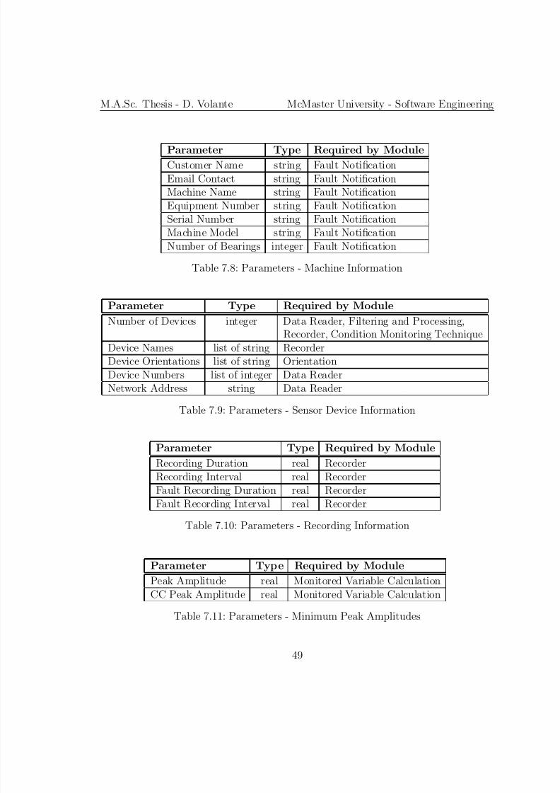
The Monitored Variable Calculation module requires various data sets in orderto compute the monitored variables. The required inputs are presented in Table 7.7.One set of filtered time domain g-forces and frequency spectrum can produce themonitored variables for an individual sensor device. One cross-correlated frequencyspectrum can allow the calculation of the monitored variables pertaining to a cross-correlated device pair. The equations and algorithms used to compute the monitoredvariables are provided in Chapter 8.
Input Data Providing Module
Filtered Time Domain G-Forces Butterworth FilterFrequency Spectrums FFTCross-Correlated Frequency Spectrums Cross-Correlation
M.A.Sc. Thesis - D. Volante McMaster University - Software Engineering
7.5 Condition Monitoring TechniqueThe Condition Monitoring Technique contains two modules: the Baseline Profile
and Monitoring Algorithm module. Monitored variables computed from the Filteringand Processing module are used to populate the baseline profile, and then later usedto compare against this profile. The Monitoring Algorithm conducts the comparison,and provides results to the Condition Handler module. Full details of the ConditionMonitoring Technique are presented in Chapter 9.
At the start of a new monitoring session, the previously used baseline profile canbe retrieved from the Storage Utilities module. Alternatively, a new baseline profilecan be constructed. Both new and old baseline profiles are summarized through the
Logger module. However, only new baseline profiles are saved in full detail using theStorage Utilities module.
7.6 Condition Handler
The Condition Handler contains the procedures for responding to the MonitoringAlgorithm results. This is divided into two parts: identifying the machine status, andnotifying users accordingly.
7.6.1 Condition Status
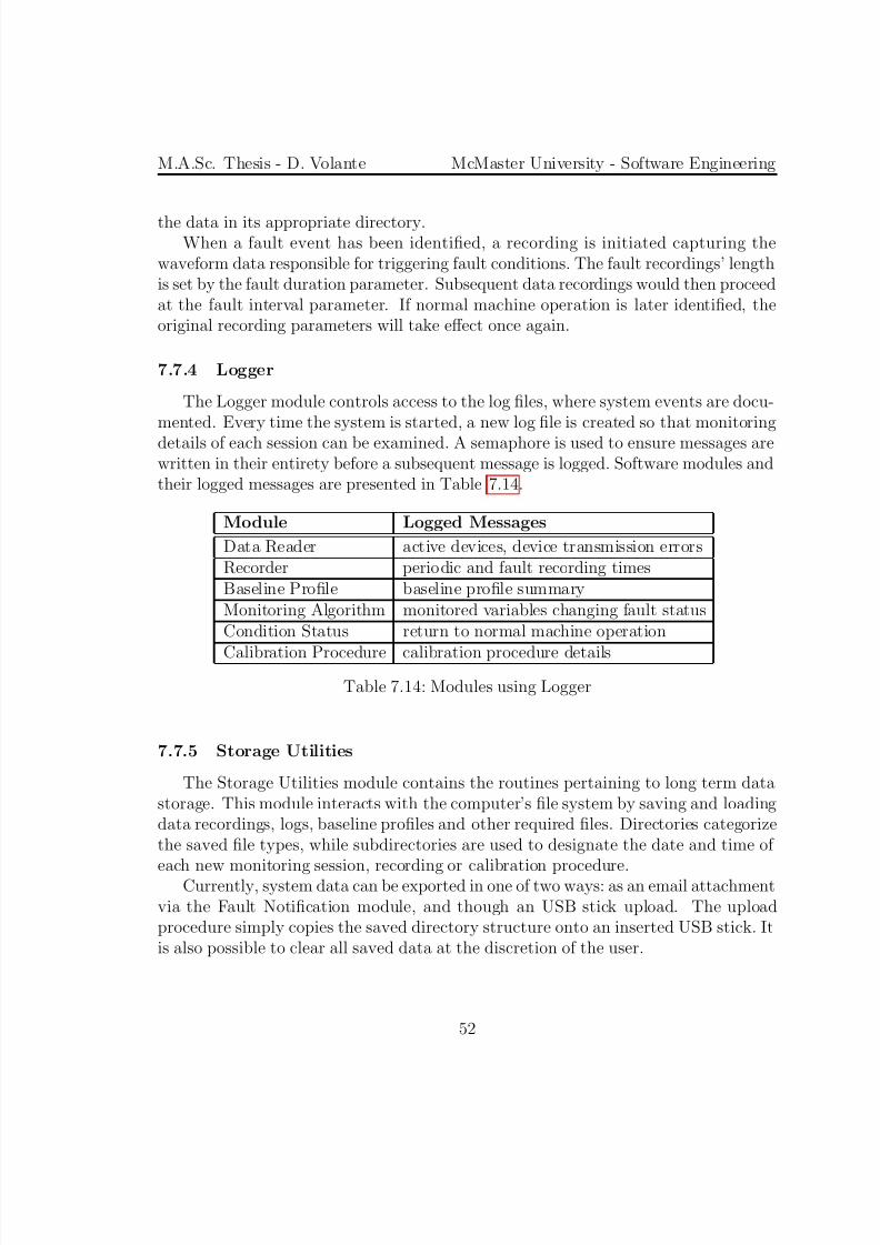
The Condition Status module identifies the condition of the vibrating screen giventhe operational status of each monitored variable. For these machines, there is cur-rently no knowledge base matching specific operational signatures to particular ma-chine faults. As a result, the machine is considered to have a fault if at least one of its monitored variables has a breached fault condition. Alternatively, a machine hashealthy or normal operation only if all monitored variables have fault-free statuses.
The Condition Status module provides the machine status to the Recorder andFault Notification modules. The Recorder uses the machine status to trigger faultrecordings and determine the rate and duration of periodic recordings. As describedin the following section, the Fault Notification module requires the machine status to
trigger its user notification procedure.
7.6.2 Fault Notification
The Fault Notification module is responsible for contacting users in the event of a machine fault. Currently, two types of user notifications exist. The first is an onscreen fault notification, with the corresponding triggered fault condition. Secondly,
M.A.Sc. Thesis - D. Volante McMaster University - Software Engineering
if the software is provided with an email address and the system with Internet access,a fault message with attached log file is emailed to the specified user.
The automatically generated emails with attachment are sent using the Mutt, asmall but powerful text-based email client. As it requires an email server, an opensource option, Postfix, was chosen. It follows the Simple Mail Transfer Protocol(SMTP) to traverse the message through the Internet to its end destination. Withthe advent of mobile computing, namely smartphones, technicians and industrial per-sonnel can access their emails remotely and immediately.
Currently, there exists future plans to interface the monitoring system with a pro-grammable logic controller (PLC), and a remote file server with a database. The
intention is to create standardized external connections, as to interface fault notifica-tions with other systems. It is the Fault Notification module that would need to beexpanded in order to implement both of these upgrades. The details of future workare discussed in Section 12.2.
7.7 Functional Modules
Functional modules are not and do not contain submodules, but rather functionand interact with other modules independently. This section contains descriptions onthese types of modules.
7.7.1 Parameter Interface
The Parameter Interface module downloads parameter files from a USB stick,and packages the parameters for module distribution. Users can create a parameterfile from a graphical user interface in the PDA software package. Transferring thisfile to the system’s monitoring computer specifies certain information required by thecondition monitoring software. The parameter file can be updated as desired to betterreflect the machine’s details and system’s operation.
Information contained in the parameter file is categorized in Tables 7.8, 7.9, 7.10,7.11, 7.12 and 7.13. Specific module parameter requirements are also identified.
M.A.Sc. Thesis - D. Volante McMaster University - Software Engineering
Parameter Type Required by Module
Customer Name string Fault NotificationEmail Contact string Fault NotificationMachine Name string Fault NotificationEquipment Number string Fault NotificationSerial Number string Fault NotificationMachine Model string Fault NotificationNumber of Bearings integer Fault Notification
Table 7.8: Parameters - Machine Information
Parameter Type Required by Module
Number of Devices integer Data Reader, Filtering and Processing,Recorder, Condition Monitoring Technique
Device Names list of string RecorderDevice Orientations list of string OrientationDevice Numbers list of integer Data ReaderNetwork Address string Data Reader
Table 7.9: Parameters - Sensor Device Information
Parameter Type Required by Module
Recording Duration real RecorderRecording Interval real RecorderFault Recording Duration real RecorderFault Recording Interval real Recorder
Table 7.10: Parameters - Recording Information
Parameter Type Required by Module
Peak Amplitude real Monitored Variable CalculationCC Peak Amplitude real Monitored Variable Calculation
M.A.Sc. Thesis - D. Volante McMaster University - Software Engineering
Parameter Type Required by Module
Main G-Force real Monitoring AlgorithmAverage G-Force X real Monitoring AlgorithmAverage G-Force Y real Monitoring AlgorithmAverage G-Force Z real Monitoring AlgorithmOperating Frequency X real Monitoring AlgorithmOperating Frequency Y real Monitoring Algorithm
Peak Frequency real Monitoring AlgorithmPeak Amplitude X real Monitoring AlgorithmPeak Amplitude Y real Monitoring AlgorithmPeak Amplitude Z real Monitoring AlgorithmCC Peak Amplitude X real Monitoring AlgorithmCC Peak Amplitude Y real Monitoring AlgorithmCC Peak Amplitude Z real Monitoring Algorithm
Table 7.12: Parameters - Tolerance Thresholds
Parameter Type Required by Module
Increment real Monitoring AlgorithmStart real Monitoring AlgorithmNormal real Monitoring AlgorithmFault real Monitoring Algorithm
M.A.Sc. Thesis - D. Volante McMaster University - Software Engineering
7.7.2 Data Reader
The Data Reader module is responsible for handling all communications with thesensor devices, as to receive the measured acceleration data. At startup, networksockets are created so incoming data is directed to the monitoring software. Giventhe parameter list of sensor devices and corresponding Internet Protocol addresses,the module then tests device network connectivity. If all devices are on the network,internally stored calibration values are individually requested, and then given to theFiltering and Processing module for later use. When the rest of the monitoringsoftware is ready, devices are simultaneous sent an acquisition start message. Thisbegins one of the main loops in the condition monitoring software.
The reader loop is contained in its own thread, as to ensure timely reception of the incoming data. When a device packet is received, an acknowledge message isreturned. This message is receipt for the sensor device, and without it the devicewill resend the packet. The packet’s structure is then examined and if correct, datais buffered to queues specific to a device and axis (X, Y, Z). These are the outputqueues where the Filtering and Processing module obtains data to be processed.
Within the Data Reader loop, malformed or missing packets trigger a transmissionerror routine. Durations between received packets are also monitored, as to handledevices that have not transmitted a packet after 2 seconds. Device silence for thisduration is indicative of a dropped packet or network failure. All these events are
documented through the Logger module. To compensate for missing data and to keepdevices synchronized, the stop data acquisition is broadcast to all devices. Devicesare reconnected, and only those that are properly networked are eligible to receivethe data acquisition start broadcast. The Filtering and Processing module is notifiedof this procedure, so it can reinitialize itself for the restarted data streams.
The Data Reader module also communicates with the Calibration Procedure mod-ule by collecting data when requested, and sending calibration values to sensor devices.The start, stop and reconnect routines are utilized on a specific device as supplied bythe Calibration Procedure module.
7.7.3 Recorder
The Recorder module governs the recording of calibrated and orientated accelera-tion data. It is given four parameters, the duration and frequency of data recordingsfor normal and faulty machine operation. Acceleration data is saved to file when duefor a periodic recording or when the Condition Status module has identified a ma-chine fault. The Storage Utilities module contains the specific procedures for saving
M.A.Sc. Thesis - D. Volante McMaster University - Software Engineering
the data in its appropriate directory.When a fault event has been identified, a recording is initiated capturing the
waveform data responsible for triggering fault conditions. The fault recordings’ lengthis set by the fault duration parameter. Subsequent data recordings would then proceedat the fault interval parameter. If normal machine operation is later identified, theoriginal recording parameters will take effect once again.
7.7.4 Logger
The Logger module controls access to the log files, where system events are docu-mented. Every time the system is started, a new log file is created so that monitoringdetails of each session can be examined. A semaphore is used to ensure messages arewritten in their entirety before a subsequent message is logged. Software modules andtheir logged messages are presented in Table 7.14.
Module Logged Messages
Data Reader active devices, device transmission errorsRecorder periodic and fault recording timesBaseline Profile baseline profile summaryMonitoring Algorithm monitored variables changing fault statusCondition Status return to normal machine operation
The Storage Utilities module contains the routines pertaining to long term datastorage. This module interacts with the computer’s file system by saving and loadingdata recordings, logs, baseline profiles and other required files. Directories categorizethe saved file types, while subdirectories are used to designate the date and time of
each new monitoring session, recording or calibration procedure.Currently, system data can be exported in one of two ways: as an email attachmentvia the Fault Notification module, and though an USB stick upload. The uploadprocedure simply copies the saved directory structure onto an inserted USB stick. Itis also possible to clear all saved data at the discretion of the user.
M.A.Sc. Thesis - D. Volante McMaster University - Software Engineering
7.7.6 Calibration Procedure
The Calibration Procedure module controls the process of calculating and savingcalibration values to a sensor device. It directs users to manipulate a device so thatdata readings can be taken at various orientations. The device’s enclosure allowsit to rest on a flat surface perpendicular to the ground, allowing each axis (±X ,±Y , ±Z ) to be parallel with gravity. For the axes, data is collected and averagedcorresponding to -1 g, 0 g and +1 g resting accelerations. Linear least squares isthen performed, where linear mappings are found from raw acceleration data to g-force values. The calibrations values, mk and bk, are saved for each axis, where themappings are expressed by the equation:
y = mkx + bk
The linear mapping is possible because the accelerometer’s datasheet specified itsoutput is linear in a defined range. Exceeding the maximum range, ± 10 g, does notguarantee output linearity.
Each sensor device requires at least one successful calibration procedure to be func-tional in the system. The calibration values are crucial to processing the accelerationdata. It is possible to recalibrate a device if the accelerometer orientation has shiftedor other sensor characteristics have changed over time. A poorly performed calibrationprocedure can result in reduced accuracy of the corresponding sensor device.
M.A.Sc. Thesis - D. Volante McMaster University - Software Engineering
8 Monitored Variables
8.1 Overview
This chapter discusses the monitored variables used in the condition monitoringprocess. These variables are calculated from the filtered waveform signals, along withthe individual and cross-correlated frequency spectrums discussed in Section 7.4.
8.2 Average G-Force
The average g-force is a monitored variable that reveals the acceleration of a
machine. Its unit is in g-forces, where 1 g equals 9.81 m/s2. It is computed for everysensor and for all three axes. Given a time window of filtered acceleration data (X ,Y or Z ), it is calculated as follows:
m averageGForcex = (| max(X )| + | min(X )|)/2
8.3 Main G-Force
Another form of average g-force is known as the main g-force. It uses filteredacceleration data from the two main drive axes, X and Y , to determine the largestg-force experienced in the corresponding plane. It is calculated as follows:
m mainGForce = max(
x2i + y2
i , ∀x ∈ X, y ∈ Y )
8.4 Operating Frequency
The operating frequency describes the speed of a periodic system in cycles persecond, commonly known as Hertz (Hz). This variable is only calculated for the Xand Y axes, as they are the only axes being driven in the vibrating machines. Since theFFT only returns a discrete set frequencies (F ) and their amplitudes (A), polynomialinterpolation is used to increase accuracy.
Given a FFT result of a time window, the operating frequency is calculated as
follows:
1. Find the largest bin amplitude (ai) and corresponding center frequency (f i)
2. Perform polynomial interpolation using the following points, (f i−1, ai−1),(f i, ai), (f i+1, ai+1), to determine the frequency corresponding to the largest am-plitude in the polynomial, which is m operatingFrequencyk
M.A.Sc. Thesis - D. Volante McMaster University - Software Engineering
While the interpolation technique is discussed in detail in [21], the implementedcalculation is expressed as follows:
α = f i+1ai−1 − f i−1ai+1 − f iai−1 + f iai+1 − f i+1ai + f i−1ai
β = f 2i−1ai+1 − f 2i−1ai − f 2i ai+1 + f 2i ai−1 − f 2i+1ai−1 + f 2i+1ai
m operatingFrequencyk = −β / 2α
Industrial end users tend to request the operating frequency in revolutions perminute, known as RPM. Since Hertz is defined as revolutions per second, the conver-sion is simply:
RPM (rev/min) = m operatingFrequencyk (rev/sec) ∗ 60 (sec/min)
8.5 Peak Frequencies
8.5.1 Peak Detection
Peak frequencies are frequencies with amplitudes that produce a local maxima inthe frequency spectrum. This process of selecting frequencies based on their ampli-tude is known as peak detection. In the monitoring system, frequencies and theiramplitudes are selected from the discrete set of FFT results for a particular axis andtime window. The FFT output either reflects the frequency content of a particular
sensor’s acceleration waveform, or is the cross-correlation of two sensors’ FFTs.The implemented detection algorithm requires a minimum peak amplitude, for
which all frequencies with amplitudes less than this value are deemed noise and thusignored. This threshold would need to be adjusted depending on the amount of noisein the monitored system.
The algorithm runs over each frequency bin, and a peak is detected if it passesboth of the following criteria:
1. The amplitude is greater than the minimum peak amplitude
2. The amplitude is greater than the four neighbouring frequencies’ amplitudes,
two from each side (greater than or equal to the subsequent bin)
This simple algorithm has been successful in identifying peaks from frequencyspectrums. However, a side effect of the second criteria is that two peaks may not bewithin three bin widths of one another. Figure 8.1 presents two successfully identifiedpeaks. This demonstrates an example of the closest two peaks can be to one another,while both being uniquely identified.
M.A.Sc. Thesis - D. Volante McMaster University - Software Engineering
Figure 8.2 depicts a similar example with two local maxima. The peaks are withinthree bin widths of one another, and as a result only the largest one will be identified.It is undesirable to have all neighbouring peaks identified, as secondary peaks withina few bins widths of the primary peak are attributed to FFT leakage or sidelobes fromthe primary peak [21].
In the Vibration Analysis Tool developed at McMaster University, a slope basedpeak detection was implemented, but the concept of ignoring peaks too close togetherwas utilized [21]. The corresponding paper empirically testing the tool, and deter-mined a peak criteria stating that peaks would only be identified if they are largerthan the next four neighbouring amplitudes. The particular tool was used in noisy
systems, but tuning all the system parameters resulted in the elimination of falsepositive peaks. The peak detection algorithm used in the monitoring system couldalso be adjusted to accommodate noisier systems, by increasing the frequency bandbetween allowable peaks.
Figure 8.1: Detecting two peaks, at 14.0 Hz and 14.4 Hz
8.5.2 Peak Assignment
Once a peak had been identified, its frequency and amplitude are then computed.Like the operating frequency computation in Section 8.4, polynomial interpolation is
M.A.Sc. Thesis - D. Volante McMaster University - Software Engineering
Figure 8.2: Detecting one peak, at 14.0 Hz
used to provide more accuracy on the frequency of interest contained in the respectiveFFT bin. Interpolation is performed using the detected peak bin values, and the two
neighbouring points. The is resulting peak frequency is assigned to m frequency.As discussed, a side effect of the FFT is that expressed amplitudes are reduced the
further away they are from their center bin frequency. An expression was derived inChapter 3 to determine the amount of amplitude reduction based on this frequencydistance. Having access to the peak and bin’s center frequency, their difference isinput into the inverse of the found expression. This function amplifies amplitudesso that the effect of FFT leakage is negated. Figure 8.3 presents an example of thescaling function for an entire bin width.
A peak’s amplitude, m amplitude, is the product of the its bin’s amplitude and theappropriate scaling factor. Scaling allows peaks to be better represented, regardless
of their location with respect to their center frequency bins. This allows peaks with adrifting frequency to have consistent amplitudes as they moves across the frequencyspectrum. Ultimately, it improves the monitorability of peaks by reducing deviationscaused by error.
M.A.Sc. Thesis - D. Volante McMaster University - Software Engineering
9 Condition Monitoring Technique
9.1 Overview
This chapter discusses the implemented condition monitoring process. The tech-nique observes monitored variables calculated from waveform data, and comparesthem to their baseline equivalent. Algorithm parameters are tuned to refine the mon-itoring process. This chapter contains the procedure and decision making techniquesthat attempt to determine the condition of the monitored variables.
9.2 Baseline ProfileBaselines are associated with normal or desired machine operation. In condition
monitoring, signals observed to deviated from the machine’s baseline typically suggestabnormal functionality. If a baseline is acquired from a machine with an existingfault, that fault would be assumed to be apart of the machine’s normal operation.This would allow the fault to go undetected, until the fault’s signature differs fromhow it was observed in the baseline. Consequently, it is assumed that baselines willbe taken from machines without faults, or at least with faults in early stages that aretoo difficult to detect using the current available technology. Technicians have accessto the Vibration Analysis Tool [21], enabling them to analyze the current status of
the machine and ensure no detectable faults are present.For the monitoring system, the baseline profile is comprised of the monitoredvariables as discussed in Chapter 8. This allows for direct comparison between thecurrent variables of the machine and its baseline, one variable at a time. To ensurethe baseline profile properly represents the operation of the machine, the machine ismonitored for multiple time windows. This allows averaging techniques to be utilized,ultimately increasing the accuracy and precision of the baseline profile.
The baseline profile for a sensor’s average g-forces, m averageGForcek and m mainGForce, are determined by taking the mean of the respective monitored vari-ables for each time window of the baseline. Since the g-forces variables already rep-resent averages, noise does not have a large impact on their values. Averaging across
the time windows further reduces the effect of system noise in their profile.The baseline operating frequency, m operatingFrequencyk, and peak frequencies,
m peakListk, are not averaged directly like the g-forces. Instead, the FFT resultsfrom the individual sensors as well as the cross-correlated sensor pairs are averagedacross their respected time windows. Operating frequencies are then calculated fromthe spectrums, using the documented methods. The frequency spectrums are then
M.A.Sc. Thesis - D. Volante McMaster University - Software Engineering
passed through the peak detection algorithm to identify peak frequencies. Since noiseis assumed to be Gaussian it affects each time window differently, so averaging theFFTs from multiple windows attenuates this noise. This procedure provides a betterrepresentation of not only the amplitudes dominated by noise, but also the amplitudesof meaningful frequency content.
9.3 Monitoring Algorithm
The implemented condition monitoring algorithm is generic in nature, able to beused in a variety of situations. It is a numeric point based system, where points are
awarded for incidents, and withdrawn when tolerances are not exceeded. An incidentevent occurs when a monitored variable exceeds its assigned threshold tolerance ina time window. The points were documented as i incidentPoint m, and known asincident points (IP). The monitoring algorithm can possibly incremented or decre-mented the IPs every time window. Each monitored variable has its own IP variableassociated with it for every sensor device and axis.
The algorithm has parameters, which are tuned to achieve the desired monitoringresponse. These parameters dictate the usage of the monitoring system. Other valuesused in the algorithm are predefined constants, and are references when determiningthe parameters. Table 9.1 presents the constants and their values, while Table 9.2presents the parameters and their corresponding restrictions.
Name Symbol Value
Decrement P dec -1Minimum P min 0
Table 9.1: Algorithm Constants
Name Symbol Restriction
Increment P inc P inc > 0Start P start P min < P start ≤ P max
Normal P norm P min ≤ P norm < P faultFault P fault P norm < P fault ≤ P max
M.A.Sc. Thesis - D. Volante McMaster University - Software Engineering
The constants and parameters are reference points and triggers for the IP val-ues corresponding to the monitored variables. Their application is depicted in thealgorithm’s framework, as presented in Figure 9.1. As previously mentioned, themonitoring process begins after the baseline profile has been determined. Monitoredvariables’ IP values are then initialized to Minimum, which is also the lower bound forIP values. The fault flag, i faultFlag m, is also initialized to false, indicating that themachine has healthy or normal operation. When a monitored variable is calculatedfor a new time window, it is then compared to the baseline profile as outlined inSection 9.4. The control flow then follows one of the two main branches, determinedby whether the tolerance threshold was exceeded or not.
If the tolerance was exceeded, and the corresponding IP value was at the Minimumvalue, the IP would be assigned the Start value. Otherwise, the IP value would beincremented by the Increment value. It is possible to assign the same value to boththe Start and Increment value, which would result in the equivalent IP value whenoriginating from the Minimum. However, if the user wants to take full advantage of the continuous monitoring, the Start value would be given a value equal to or greaterthan the Fault value. Doing so would allow a single deviation from the baseline toimmediately trigger a fault condition (IP ≥ P fault), given that the corresponding faultcondition is not already in process. This results in the documentation of any abnormalmachine event.
Due to the presence of noise in a monitored system, it may not be desirable to
allow a single incident to activate a fault condition. In this situation, Start would beassigned a value less than Fault. In order to trigger a fault, a monitored variables’stolerance would need to be breached over multiple time windows. The minimumnumber of time windows required to indicate a fault (MT W min-fault) can be calculatedas follows:
MT W min-fault = (P fault − P start)/P inc + 1
This number is designated as a minimum because it is not a requirement that thetolerances be exceeded in consecutive time windows. It is possible that a monitoredvariable causing incidents would not trigger its tolerance for a few time windows
within its progression to activating the fault condition. In such time windows, thecontrol flow would follow the second of the two main branches.
The second main branch in the monitoring algorithm manages the incident pointsin time windows where a monitored variable does not deviate from the baseline. Thesimplest case for the branch is when a monitored variable’s IP value is at the Minimum,and no action needs to be taken until the next time window. Alternatively, an IP
M.A.Sc. Thesis - D. Volante McMaster University - Software Engineering
with a value greater than the Minimum will be altered by Decrement. Note that valuescannot be decremented below Minimum, as enforced by the algorithm.
Unlike the Increment value, the Decrement has a constant value of -1. The sig-nificance of Decrement’s magnitude is equivalent to the duration of one time window.For any given monitored variable, the summation of the acquired IP represents theminimum number of time windows that variable must remain within its tolerancein order to return to Minimum. This is also considered a minimum number becauseconsecutive equivalent actions are not required. More importantly, if a monitoredvariable has an activate fault condition, the minimum number of non-deviating timewindows required to signify a return normal operation is simply:
MT W fault-norm = P fault − P norm
This presents the purpose of the Normal value, a trigger threshold to set the faultflag to false when the current IP is less than or equal to its value. Note that thecorresponding monitored variable must also have an active fault condition, indicatedby the fault flag being true.
It is possible that abnormal machine operation is temporary, and so the monitoringalgorithm will identify when fault symptoms are alleviated beyond detection. After afault is detected, the capacity to return to normal operation is expressed through thedifference between the current IP value and Normal, denoted by MT W IP-norm. Theupper bound to this minimum number of non-deviating time windows is restricted bythe Maximum value. A monitored variable whose IP value exceeds the fault trigger canstill be incremented up until Maximum if the fault continues to persist. As a result,the upper bound to MT W IP-norm can be determined by:
max(MT W IP-norm) = P max − P norm
The collection of minimum time windows (M T W s) provides additional numericalindicators on how the algorithm is being utilized. This can aid users and techniciansby emphasizing the relationships between the chosen parameters.
M.A.Sc. Thesis - D. Volante McMaster University - Software Engineering
9.4 Tolerance ThresholdsFollowing the calculation of a baseline profile, the monitored variables of each
subsequent time window are compared to their respective baseline value. This stepsimply determines if a variables’s current time window value is within an acceptabledeviation from the baseline profile. For g-forces and frequency amplitudes, a relativedifference is used, whereas for frequencies an absolute difference is utilized.
Users and technicians must select deviations for each type of monitored variableand axis in m machineProfile. These deviation allowances are known as trigger orthreshold tolerances. When a monitored variable’s value exceeds its tolerance in atime window, the event is referred to as an incident and does not necessarily imply
abnormal machine operation. Rather, this is determined by the implementation of the monitoring algorithm, as outlined in the previous section.
It should be noted that the current implementation attempts to minimize thenumber of parameters as to simplify usability for end users. The monitoring system’salgorithm could be revamped so that frequency peaks with different amplitudes areassigned different tolerance thresholds. Absolute tolerance thresholds could also beadopted for peak amplitudes, but would also require additional tuning for the variousamplitudes.
9.5 Baseline Profile Stability
As mentioned, it may be desirable to select parameters such that a single viola-tion of a tolerance threshold (an incident), would not trigger a fault condition. Thethreshold would instead have to be exceeded for at least the minimum number of timewindows to indicate a fault, MT W min-fault. The benefit of the described usage is inthe reduction of potential false positive faults caused by noise. As noise is random,it is unlikely that it would cause persistent deviation of a specific monitored variablefrom its baseline profile across multiple time windows.
In noisy environments it is expected that false positive incidents would occur whenthe system is given a set of tolerance thresholds with a close bound to the baselineprofile. Desired system performance can be achieved provided noise based incidents
do not exceed the weighted ratio of the Decrement to Increment, as reflected by:
|P dec| : P inc
With a 1:1 ratio, time windows that do not deviate from the baseline would coun-teract incidents, using an equivalent weighting. Despite an evenly distributed 50 % in-
M.A.Sc. Thesis - D. Volante McMaster University - Software Engineering
cident rate, a monitored variable’s incident point value would remain near the Minimumvalue. For fault detection, consistance readings across time windows would be heavilyfavoured.
Using a different ratio where P inc is greater than |P dec| would function like previ-ously discussed yet allow for a larger impact from incidents. In situations where mostnoise deviations are contained within the tolerance threshold, a large Increment valuewould acknowledge the significance of a subsequent incident. Specifically, it would re-quire Increment time windows of normal operation to completely counterbalance oneincident.
It should be mentioned that Start can be assigned a different value than
Increment so that the first of a potential train of incidents can have its own weighting.It is up to technicians to decide if this weighting should smaller, larger, or simplyequivalent to any other incident.
In general, if noise is high enough to trigger a fault condition, the monitoringsystem would require tuning for successful operation. End user action from at leastone of the following would need to be taken:
1. Increase the tolerance threshold of the corresponding monitored variable, as toreduce the frequency of noise triggering the threshold
2. Decrease Start so that isolated incidents are not as heavily weighted
3. Decrease Increment so that more consistency is required for fault detection
4. Increase Fault to reduce the likeliness of the fault condition being breachedby clusters of incidents, by allowing more opportunity for non-deviating timewindows to counteract the noise-based incidents
5. Increase the minimum detectable peak amplitude so that the baseline profilewould disregard smaller peaks encompassed by noise
M.A.Sc. Thesis - D. Volante McMaster University - Software Engineering
10 Monitoring Simulation
10.1 Overview
This chapter presents a simulation of a vibrating machine that is monitored bythe condition monitoring system. A stable baseline profile will be first be determined.Faults will then be introduced into the machine to determine the effectiveness of thesoftware system. The system will operate at 500 Hz sampling and use 4096 points inthe FFT calculations. Only the X-axis will be discussed, as analogous methodologiesare utilized for the Y and Z axes.
10.2 Simulated Signals
The simulated signals of a healthy vibrating machine are constructed using sinu-soidal waves of various frequencies and amplitudes. Like the real vibrating machines,a dominant frequency is present representing the operating frequency. Noise is alsoincluded into the signals to reflect potential inaccuracies of the sensors as well thematerial flow over the machine. Gaussian random noise with a mean of zero andstandard deviation of one, N (0, 1), was chosen for this role. The experiment is con-ducted using four virtual sensors, where the amplitudes of the sinusoidals in eachsignal are presented in Table 10.1.
M.A.Sc. Thesis - D. Volante McMaster University - Software Engineering
10.3 Baseline ProfileThe first assessment on the monitoring system was ensuring a successful construc-
tion of the baseline profile for the simulated machine. Half an hour of generatedwaveform data (900,000 points) was passed into the monitoring system. The firstminute of data is used to establish the baseline profile, while the remaining datawould be monitored to confirm its stability. The minimum peak amplitudes, tol-erance thresholds and algorithm parameters chosen to identify a stable profile arepresented in Table 10.2. Empirical testing was used to refine these values. The se-lected parameters were not exhaustively optimized for the given monitored machine,as to better reflect the practical use of the system by end users.
Minimum Peak AmplitudesIndividual Peaks 0.10
Cross-Correlated Peaks 0.006
Tolerance ThresholdsAverage G-Force 5.0%
Operating Frequency 0.050 HzPeak Frequency 0.061 HzPeak Amplitude 10.0%
Cross-Correlated Peak Amplitude 30.0%
Algorithm ParametersIncrement 1
Start 1Normal 0Fault 8
Maximum 8
Table 10.2: Selected System Parameters
The numeric values of the parameters reveals the fairly conservative use of themonitoring system as detailed in Section 9.3. A single violation of a tolerance thresh-old in a time window, known as an incident, would not trigger the fault condition.Rather, it would have to be exceeded for at least the minimum number of time win-dows to indicate a fault, MT W min-fault. For the simulation, this duration is eight timewindows, corresponding to approximately a minute. The implementation is targetedtowards the monitoring of sustained abnormalities and faults.
M.A.Sc. Thesis - D. Volante McMaster University - Software Engineering
The individual sensors’ baseline profiles of the simulated machine are presentedin Table 10.3. The frequencies of interest were all successfully identified, withoutthe inclusion of any extraneous frequency content. All sensors also independentlyand correctly identified 14.03 Hz as the operating frequency of the machine. Thebaseline profile is also comprised of peak frequencies detected from the cross-correlatedfrequency spectrums, as provided in Table 10.4.
Peak Frequency / AmplitudeSensor 14.03 Hz 22.97 Hz 35.03 Hz 41.99 Hz Average G-Force
Table 10.4: Simulated Machine’s Baseline Profile - Cross-Correlated Peaks
After establishing the baseline profile, no faults conditions were triggered whilemonitoring the remainder of the normal machine operation. However, it was seenfrom the incident point values in the monitored variables that incidents did occur.The most susceptible variables to noise based incidents were the peak frequencies
with low amplitudes, specifically the 42.0 Hz peaks. With a 10 % peak amplitudetolerance threshold, small amplitudes are not given as much of an absolute deviationfrom the baseline profile as compared to larger peak amplitudes. If this did causebaseline profile instability, Section 9.5 presents different approaches to supressing thesystem noise.
M.A.Sc. Thesis - D. Volante McMaster University - Software Engineering
10.4 Emerging Frequency ContentThe first set of simulated faults introduce additional frequency content into the
machine’s normal operation. As discussed in Section 2.2, emerging peak frequenciesare evidence of various machine failures in gears, bearings, shafts, springs or othercomponents that contribute vibrations.
10.4.1 Visible Content
In this experiment a sinusoidal wave of 28.0 Hz is added to each sensor’s signal,with the corresponding amplitudes shown in Table 10.5. The fault induced frequency
spectrum of the RFB signal is presented in Figure 10.3, where the new peak frequencyis visible.
In the machine’s signals, the fault persisted for 20 time windows. All four sen-sors and six cross-correlations were able to identify an emerging peak frequency at27.97 Hz. Table 10.6 contains the reported amplitudes, which indicate the fault hadthe greatest effect near the LFB sensor location. If this was an unknown fault on areal machine, it would be advised technicians investigate the LFB area of the machinefor a damaged component.
M.A.Sc. Thesis - D. Volante McMaster University - Software Engineering
Figure 10.3: RFB Frequency Spectrum, containing simulated 28.0 Hz fault
After successful identification of the fault, its signature was removed from themachine’s signal to reflect a temporary abnormality or machine maintenance. The
experiment was continued to ensure the monitoring system was able to detect theabsence of the fault. Shortly after eight time windows, as determined by P fault-norm,the monitoring system correctly identified that the simulated machine was runningunder normal operation once again.
10.4.2 Buried Content
Similar to the previous experiment, frequency content was introduced into themachine’s healthy signals. A 57.0 Hz sinusoidal wave was used, with amplitudespresented in Table 10.7. The entire monitored frequency spectrum of the sensorscontaining the largest fault amplitudes, RDB and LDB, are presented in Figures 10.4and 10.5. In this situation, it is unlikely technicians would be aware of the emergingpeaks through visual inspection of the frequency spectrum. Each sensors’ amplitudecorresponding to 57.0 Hz are visually concealed by the noise of the system.
The 57.0 Hz sinusoidal fault signals were introduced for 50 time windows. Noindividual sensor was able to detect the emerging frequency content for the dura-tion of the experiment. However, peak detection from the cross-correlated frequency
spectrums were able to identify the peak frequency of interest in two instances, as
presented below in Table 10.8. The common element between the two cross-correlatedfrequency spectrums is the RDB sensor, indicating the fault likely originates in thatregion of the machine. When the fault signature was removed from the machine’ssignal, the monitoring system successfully identified normal machine operation.
Faults identified solely through these means do not appear critical, as their con-tributed vibration amplitudes is minimal. However, they are indicators of futuremachine health and an advisory requesting maintenance. Once fault signatures arerecognized, an expert system could give end users detailed recommendations regardingthe severity of the particular fault.
M.A.Sc. Thesis - D. Volante McMaster University - Software Engineering
10.5 Lost Frequency ContentThe simulated fault in this experiment is the withdrawal of the 35.0 Hz peak
frequency from the RFB’s normal signal. This signifies the failure of an auxiliarycomponent, where the machine continues to operate with the loss of some function-ality. Due to the rigid body of the vibrating machines, the 35.0 Hz peak was notcompletely removed, but rather only 25 % of the assigned amplitude remained. Theresidual vibration caused from similar functioning components on other parts of themachine would induce some amplitude of this frequency content.
The abnormal frequency spectrum is presented in Figure 10.6. The peak frequencywas reduced for 10 time windows, and then reintroduced at its corresponding baseline
amplitude. The fault condition was triggered when the system identified a 76 %amplitude reduction of the 35.0 Hz peak at the RFB location. Such a reductionwould be cause for a machine inspection at the indicated location. When the 35.0 Hzpeak returned to its proper amplitude, the system declared normal operation.
Figure 10.6: RFB Frequency Spectrum, with a reduced 35.0 Hz peak
M.A.Sc. Thesis - D. Volante McMaster University - Software Engineering
10.6 Changing G-ForcesThis experiment simulates another form of undesired operation, machine unbal-
ance. When vibrating screens are properly weighted, acting g-forces are consistentthroughout the machine. This allows the entire surface of the screen to be equallyeffective. If properly balancing is not achieved, different portions of the screen expe-rience different g-forces. The result of the unexpected g-forces is irregular materialscreening and potential damage to the machine.
To simulate this fault scenario, the RFB location has an increased operationalamplitude while LDB has a reduced amplitude. Table 10.9 presents the absolute andrelative amplitude changes from 14.0 Hz sinusoidals used in the production of the
baseline signals. Frequency spectrums from the fault induced sensors are given inFigure 10.7 and 10.8.
Difference from Baseline ProfileSensor Location Absolute (g) Relative (%)
The fault condition was triggered when monitoring the 20 time windows of ab-normal operation. The average g-force tolerance threshold was exceeded by both theRFB and LDB sensors. Table 10.10 presents the observed fault signature. No specificfrequency was identified, but it is known that large deviations amongst sensors’ g-forces are associated with unbalance. Adding weight to specific parts of the machinecan allow for a more uniform operation.
Exceeded Average G-ForcesSensor Location Amplitude (g) Relative Difference (%)
RFB 3.88 7.51LDB 3.24 -6.22
Table 10.10: Simulation Results - an Unbalanced Machine
M.A.Sc. Thesis - D. Volante McMaster University - Software Engineering
It should be noted that the operating frequency’s peak amplitude did not triggera fault condition. The 14.0 Hz peak seen in Figure 10.7 is visibly larger than in thebaseline, as seen in Figure 10.2. However, the difference remained consistently lessthan the selected 10 % tolerance threshold and so no corresponding fault condition wastriggered. If it was desired to have this variable trigger a fault at the given amplitude,one would have to decrease the peak frequency amplitude tolerance threshold. Thiswould allow smaller deviations to be considered incidents for all the correspondingaxial peak amplitudes.
10.7 Drifting Operating Frequency
The simulated fault in this experiment is a drift in the operating frequency. A0.095 Hz increase is induced into the vibrating machine for 25 time windows. Thisabnormality is large enough to violate the selected tolerance threshold put on theoperating frequency.
When performing the experiment, fault conditions were successfully triggeredwhen the monitoring system identified a consistent change in the operating frequencyfor all sensors. Table 10.11 presents the unanimous input and detected operatingfrequency for the baseline profile and current experimental fault signal.
Table 10.11: Simulation Results - Drifting Operating Frequency
The RFB frequency spectrum with drifted operating frequency is presented inFigure 10.9. When visually compared to the baseline’s spectrum, Figure 10.2, a largereduction in the operating frequency’s peak amplitude is seen. This is further evidenceof the FFT leakage discussed in Chapter 3, as the input amplitude was not reducedbut rather shifted in the frequency axis. If the system did not account for this as in
Section 8.5, then it would have also concluded there was a reduction in amplitude.After the fault was detected, the operating frequency was returned to the observed
baseline profile. The system was able to identify the return to the original operatingfrequency for all sensors, and then declared normal machine operation.
M.A.Sc. Thesis - D. Volante McMaster University - Software Engineering
Figure 10.9: RFB Frequency Spectrum, with drifted operating frequency
10.8 Noise-Based Faults
In this last experiment set, the fault signals remain the same as the simulated base-line signals with the exception of increased noise. For a vibrating machine increasedlevels of noise are expected signatures of screening larger aggregates, structural deteri-oration from extensive operation, or active environmental conditions. To reflect such,the initial Gaussian random noise, N (0, 1), was amplified as presented in Table 10.12.
Gaussian Random NoiseSimulation Notation Mean Standard Deviation
Baseline Signal N (0, 1) 0 g 1.0 gExperiment 1 N (0, 2) 0 g 2.0 gExperiment 2 N (0, 3) 0 g 3.0 gExperiment 3 N (0, 5) 0 g 5.0 g
Table 10.12: Noise Experiments - Gaussian Random Noise
M.A.Sc. Thesis - D. Volante McMaster University - Software Engineering
10.8.1 Noise Experiment 1
For all three noise experiments, half an hour of simulated waveform data was mon-itored. The first experiment uses signals with N (0, 2) noise, and the correspondingfrequency spectrum up to 100 Hz for a time window is presented in Figure 10.10.
Figure 10.10: RFB Frequency Spectrum, with N (0, 2) noise
The monitoring system detected increased average g-forces for all sensors, as pre-sented in Table 10.13. For this monitored variable, all sensor locations experienced asimilar effect, ranging from a 13 to 16 % increase. Increasing the noise can increasethe energy of the system, allowing it to output more g-forces.
Exceeded Average G-ForcesSensor Location Absolute (g) Relative Difference (%)
M.A.Sc. Thesis - D. Volante McMaster University - Software Engineering
Another type of detected fault condition was the deviation of the smallest peakamplitude from the baseline profile. Table 10.14 presents the corresponding 42.0 Hzpeak amplitudes. The RFB sensor location has multiple values recorded, as over thecourse of the experiment it returned to acceptable levels, as denoted by ’a’. TheRFB 42.0 Hz peak amplitude triggered its fault condition three times throughoutthe experiment. This repeated fault triggering, especially with the amplitude beingtoo large then too small, and accompanying increased g-forces are strong evidence of noise.
In this experiment, the same procedure will be carried out as in the previoustest. However, noise will be increased to N (0, 3). Figure 10.11 presents the frequencyspectrum up to 100 Hz for a time window of the signal.
As expected, all average g-forces exceeded the tolerance threshold. Table 10.15presents the increased averages, ranged from 26 to 32 %, roughly doubling the relativedifferences from the previous experiment.
Exceeded Average G-ForcesSensor Location Absolute (g) Relative Difference (%)
RFB 4.56 26.2LDB 4.37 26.4
RDB 4.85 28.9LFB 4.49 31.5
Table 10.15: Simulation Results, Average G-Forces - N (0, 3) Noise
M.A.Sc. Thesis - D. Volante McMaster University - Software Engineering
Figure 10.11: RFB Frequency Spectrum, with N (0, 3) noise
Individual and cross-correlated peak amplitudes were also seen deviating fromtheir baseline profile. Table 10.16 presents the individual sensors’ breached fault
conditions. It was the three smallest peaks from the baseline profile that were mostaffected by the noise. All deviated amplitudes for the 23 and 35 Hz peaks returned toacceptable levels, where some went on to trigger a fault condition again. Alternately,all the 42 Hz peaks were completely influenced by noise, continuously maintainingtheir fault status.
M.A.Sc. Thesis - D. Volante McMaster University - Software Engineering
10.8.3 Noise Experiment 3
The final noise experiment further increases the used noise to N (0, 5). Figure 10.12depicts the strength of the noise across the frequency spectrum of a time window.
Figure 10.12: RFB Frequency Spectrum, with N (0, 5) noise
When monitoring the noisy signal, average g-forces exceeded relative tolerances inthe range from 55 to 63 %. Table 10.17 presents these findings.
Exceeded Average G-ForcesSensor Location Absolute (g) Relative Difference (%)
RFB 5.58 54.7LDB 5.36 55.0RDB 5.99 59.1
LFB 5.58 63.3
Table 10.17: Simulation Results, Average G-Forces - N (0, 5) Noise
Again, the three smallest individual and cross-correlated peak amplitudes wereseen deviating from the baseline profile. Some of the peaks were undetectable as a
M.A.Sc. Thesis - D. Volante McMaster University - Software Engineering
result of the noise. Table 10.18 presents the individual sensor results, denoting un-detectable peaks with an ’L’, to indicate they are lost frequency content. Noise haseither diminished their amplitudes below the minimum peak amplitude, or neighbour-ing noise-based peaks are dominating their presence.
Some of the peak amplitudes were identified as too large, but would return toacceptable operational amplitudes. This was followed by two other triggers, indicatingamplitudes were reduced beyond the tolerance.
Like the other noise-based experiments, similar fault signatures are seen. It wasalso observed that increasing the levels of noise increases the effect of the correspond-ing symptoms. In summary, signatures of increased levels of noise are:
• increased average g-forces• repeated triggering of peak amplitudes
• peak amplitudes that are too large, becoming too small (and vise-versa)
M.A.Sc. Thesis - D. Volante McMaster University - Software Engineering
11 System Testing
11.1 Overview
This chapter documents the system testing performed on an in-house vibratingscreen. After a stable baseline profile is constructed experiments are carried out, eachimitating a fault condition. The monitoring software in combination with the systemnetwork and sensor devices will be examined in an industrial setting. The system willoperate at 500 Hz sampling and use 4096 points in the FFT calculations.
11.2 Test MachineThe machine monitored in the testing process is a linear vibrating screen. This
type of machine uses linear motion to quickly screen large amounts of material. Fig-ure 11.1 presents a side view, while Figure 11.2 presents a discharge end view.
Figure 11.1: Linear Vibrating Screen - Side View
The vibrating screen is driven by two motors, as seen from the discharge endview. The machine is also equipped with a variable-frequency drive (VFD). VFDscontrol the frequency of electrical power supplied to a motor, which in turn affects the
M.A.Sc. Thesis - D. Volante McMaster University - Software Engineering
Figure 11.2: Linear Vibrating Screen - Discharge End View
rotational speed of the motor. This allows the operational frequency of the machineto be tuned while running.
Also visible from the discharge end view is a slotted wooden box bolted to thevibrating screen. During testing it housed rocks to imitate the material flow. Thebox itself was seen vibrating, contributing additional noisy content.
Only two Wi-Fi prototype sensor devices were constructed, so the number of sensors used in system testing was limited. The sensor devices were placed on bothsides of the discharge end body, denoted as RDB and LDB.
11.3 Baseline Profile
While constructing a stable baseline profile for the X and Y axes was relativelysimple, the Z-axis proved to be more challenging. The vibrating screen’s motors
rotates in the XY plane, governing motion in those axes. Figure 11.3 presents theX-axis acceleration for a quarter time window. Figure 11.4 contains the correspondingbaseline frequency spectrum. Both sensors’ X and Y axes appear similar in nature; asingle operating frequency peak with little noise and no other spectrum content.
M.A.Sc. Thesis - D. Volante McMaster University - Software Engineering
Noise and other frequency content was observed in the Z-axis. The accelerationwaveform of the LDB Z-axis is presented in Figure 11.5. The sensor devices’ frequencyspectrums reveals the contained content, as seen in Figures 11.6 and 11.7. Many of thevisible Z-axis peaks were not consistently present, and would trigger a fault conditionwhen monitored. This required the minimum peak amplitude to be greater than theinconsistent peaks.
Figure 11.5: Baseline LDB Z-Axis Waveform
The selected parameters used to construct the stable baseline profile are presentedbelow in Table 11.1. Empirical testing refined these values over a few attempts. Theresulting baseline profile is presented over Tables 11.2 and 11.3. All sensors devicesreported 14.94 Hz as the operating frequency of the vibrating screen.
11.4 Loose ComponentsWhile the constructed baseline profile was deemed stable, the LDB Z-axis peak
at 157.98 Hz occasionally trigged its fault condition when the machine was restartedbetween experiments. At times the particular baseline profile peak would disappear,while a new peak would emerge nearby. Peaks up to 164.54 Hz were seen emergingreplacing the original peak. Figure 11.8 presents the altered LDB Z-axis spectrum.
M.A.Sc. Thesis - D. Volante McMaster University - Software Engineering
Such a shift in frequency indicates a loose component on the machine that issusceptible to changing its rotational path. Since the test machine was in good healthaside from the induced faults, the unknown fault condition was attributed to themounted wooden box containing the aggregate. Unlike any other part of the machine,the bolts mounting the box were loose and able to vibrate. Nonetheless, it providedan experimental example of signatures pertaining to loose components.
11.5 Induced Impacts
In this experiment the vibrating screen was subject to impacts caused by a wooden
block placed in its path. The impacts occurred on the left discharge end body, nearthe LDB sensor. Such impacts could be caused by loose or damaged components.Alternately, when aggregate material builds up it can overflow and obstruct machinemovement.
The impacts were introduced until the fault signature was revealed. As a result of the impacts, the LDB sensor experienced increased noise, as presented in Figure 11.9.The triggered fault condition was due to increased average g-forces, as presentedTable 11.4.
Figure 11.9: LDB X-Axis Frequency Spectrum, with induced impacts
M.A.Sc. Thesis - D. Volante McMaster University - Software Engineering
Exceeded Average G-ForcesSensor Axis Amplitude (g) Relative Difference (%)
LDB Main 5.97 8.54X 4.64 15.71Z 0.729 142.19
Table 11.4: Fault Conditions - Induced Impact
After the faults were detected, the wooden block was removed from the vibratingscreen’s path. The system was able to correctly identify that the vibrating screen was
back to normal operation.
11.6 Motor Failures
As mentioned, the linear vibrating screen is driven by two electric motors. If afailure occurs on one of the two motors, the screening efficiency would be drasticallyreduced. If both motors fail, the vibrating screen ceases to move. This experimentset monitors single and double motor failures.
11.6.1 Single Motor Failure
The single motor failure was induced by simply removing power from the topmounted motor. There were numerous triggered fault conditions; Table 11.5 presentsthe g-force based faults conditions. The average g-forces in the Y-axis were diminished,yet the X-axis g-forces were slightly increased. Ultimately, less vibrational g-forceswere being produced.
Exceeded Average G-ForcesSensor Axis Amplitude (g) Relative Difference (%)
LDB X 4.27 6.48Y 3.35 -12.30
RDB X 4.18 6.91
Y 3.21 -12.77
Table 11.5: Fault Conditions - Single Motor Failure
Another set of experienced fault conditions was the unanimous detection of a driftin operating frequency by -0.05 Hz. It is intuitive that the loss of a motor would slow
M.A.Sc. Thesis - D. Volante McMaster University - Software Engineering
down the machine’s movement. After the faults were realized, power was restoredto the motor where the monitoring software quickly identified the return to normaloperation.
11.6.2 Double Motor Failure
In this experiment, power to both motors on the vibrating screen was removed.In this state, the machine is inoperative. All baseline profile peaks were no longerdetectable, and experienced average g-forces all reported minimal values.
Interestingly, the LDB sensor reported an operating frequency of 60.04 Hz, whilethe RDB reported 177.0 Hz. These values are either the product of noise in the sensorcircuitry or the industrial environment.
11.7 Machine Unbalance
A technique used to imitate a spring failure involves unbalancing the vibratingscreen. This was achieved by raising the base frame of the machine on three cornersand letting the fourth corner sag. For this experiment, the LDB corner remained onthe ground.
The only detected fault condition was the absence of the 156.98 Hz peak from theLDB Z-axis. While it was mentioned that this peak was susceptible to movement
across the frequency spectrum, no other experiment had this content completely re-moved. Figure 11.10 presents the modified Z-axis frequency spectrum of the LDBsensor.
11.8 Drifting Operating Frequency
This experiment drifts the operating frequency of the vibrating screen while it isactive. An altered operating frequency could be attributed to changing dynamics of the vibrating screen, and is also an indicator of reduced efficiency. Machine vibrationsare tuned for certain materials and screen sizes, and shifting away from the desiredcharacteristics only degrades performance.
To drift the operating frequency, the variable-frequency drive (VFD) was used toincrease the frequency of the power signal. The inputs and unanimously detectedoperating frequencies are presented in Table 11.6.
The operating frequency was slowly decreased until the monitoring system iden-tified a breached fault condition. The first operating frequency to trigger a fault,15.0 Hz, exceeded the threshold tolerance placed on the baseline profile.
Table 11.6: Results - Drifting Operating Frequency
After the fault notification, the original operating frequency was restored. Themonitoring system was able detect the operation had returned to the baseline profile.
11.9 Network Performance
Over the course of the fault experiments, the communication network between
the sensor devices and monitoring computer was observed. Only in two instancesthroughout the testing day did a sensor send a malformed packet. The monitoringsystem was able to automatically restart communications within seconds, quicklyresuming the monitoring process. The monitoring system’s network proved to bereliable and robust.
It is expected that manufactured sensor devices with surface mount components
M.A.Sc. Thesis - D. Volante McMaster University - Software Engineering
will have increased performance compared to the current prototype. Electrical pathscan be optimized, and contacts between components will be enhanced. As suggestedby the WiFly datasheet, an improved layout would maximize distance between theWi-Fi module and any metallic mounting bracket.
M.A.Sc. Thesis - D. Volante McMaster University - Software Engineering
12 Conclusion
12.1 Discussion
This thesis presented the design, implementation and testing of a condition moni-toring system for use on vibrating screens. The system was able to collect accelerationdata from remote sensor devices as to construct a baseline profile of a machine. Sub-sequent data from operation was then compared to this profile for fault detectionpurposes. Fault signatures were detected and recorded through various experiments.A discussion will be carried out evaluating the performance of the hardware andsoftware system components.
The upgraded hardware utilized in the monitoring system proved to be success-ful. The sensor devices equipped with Wi-Fi modules performed better than theirBluetooth equivalents. The wireless network hosted by the router allowed for in-creased transmission rates over larger distances, with an increased node capacity.Transmissions errors were very rare, and the system was able to easily resynchronizecommunications.
The monitoring computer was able to reliably communicate with the sensor devicesthrough the network, allowing acceleration data to be supplied to the monitoringsoftware. The computer was easily interfaced with other networks and computers,and when given Internet access could autonomously send email fault notifications
providing users with a log file.The monitoring software successfully constructed stable baselines profiles and de-tecting various fault conditions. For both virtual and live industrial experiments,minor tuning of the system parameters achieved the desired monitoring response.System testing revealed the monitoring technique could be utilized in a practicalindustrial setting.
Slight modifications to the monitoring software could allow for finer tolerancethresholds to be put on the monitored variables. Due to the nature of the vibratingscreen, the X and Y axes accelerations are similar while the Z-axis is very different.As such, the Z-axis should have more independent parameters such as minimum peakamplitudes and the peak frequency range. Smaller deviation bounds could then be
placed on the X and Y axes, while Z-axis profiles can remain stable using its owntolerances.
The completed condition monitoring system is a self-contained product. However,additional monitoring and testing on more types of vibrating screens would providefurther insight on how to refine the system. The following section contains knownsuggestions on how to advance the condition monitoring system.
M.A.Sc. Thesis - D. Volante McMaster University - Software Engineering
12.2 Future WorkThis section provides a list of suggested future work to expand the scope of the
implemented condition monitoring system. The following items are recognized anddesired by the sponsoring company:
1. Introduce fault notification hardware by interfacing the monitoring computerwith a programmable logic controller (PLC). Industrial control rooms commonlyuse PLCs to control and monitor machinery. Users would have much moreflexibility when interfacing with the system.
2. Expand the condition monitoring software by increasing the number of mon-itored variables used in the machine profile. Ellipse fitting algorithms couldprovide eccentricity and phase angles of the machine rotation. New monitoredvariables would require their own tolerance thresholds.
3. Work has already begun creating a website and database so that data record-ings and fault notifications could be automatically uploaded to a centralizedserver over the Internet. This would accumulate data recordings, enabling theopportunity for long term machine analysis. It would also be possible to selectsystem parameters through a web interface, and have the monitoring computerretrieved the desired settings.
4. Once a sufficient knowledge base for fault signatures is compiled, the monitoringsystem could be provided with a mapping from deviated monitored variables tomachine faults. Instead of notifying users of the breached monitored variables,specific faults and their severity could be presented to the user. Such an upgradewould classified the monitoring system as an expert system.
M.A.Sc. Thesis - D. Volante McMaster University - Software Engineering
Bibliography[1] D. C. Baillie and J. Mathew. A comparison of autoregressive modeling techniques
for fault diagnosis of rolling element bearings. Mechanical Systems and Signal Processing , 10(1):1 – 17, 1996.
[2] Changzheng Chen and Changtao Mo. A method for intelligent fault diagnosis of rotating machinery. Digital Signal Processing , 14(3):203–217, 2004.
[3] Seung-deog Choi, B. Akin, M.M. Rahimian, and H.A. Toliyat. Fault diagnosis im-plementation of induction machines based on advanced digital signal processing
techniques. Twenty-Fourth Annual IEEE Applied Power Electronics Conference and Exposition , pages 957–963, Feb. 2009.
[4] E.H. Clayton, Bong-Hwan Koh, Guoliang Xing, Chien-Liang Fok, S.J. Dyke, andChenyang Lu. Damage detection and correlation-based localization using wirelessmote sensors. Intelligent Control, 2005. Proceedings of the 2005 IEEE Interna-tional Symposium on, Mediterrean Conference on Control and Automation , pages304 –309, jun. 2005.
[5] Stephan Ebersbach and Zhongxiao Peng. Expert system development for vibra-tion analysis in machine condition monitoring. Expert Systems with Applications ,
34(1):291–299, 2008.[6] Paul M. Frank. Fault diagnosis in dynamic systems using analytical and
knowledge-based redundancy: A survey and some new results. Automatica , 26(3),1990.
[7] D. Fuessel and R. Isermann. Hierarchical motor diagnosis utilizing structuralknowledge and a self-learning neuro-fuzzy scheme. Industrial Electronics, IEEE Transactions , 47(5), 2000.
[8] K.B. Goode, B.J. Roylance, and J. Moore. Development of model to predictcondition monitoring interval times. Ironmaking and Steelmaking , 27(1):63 – 68,
2000.
[9] A. Grall, C. Brenguer, and L. Dieulle. A condition-based maintenance policy forstochastically deteriorating systems. Reliability Engineering and System Safety ,76(2):167 – 180, 2002.
M.A.Sc. Thesis - D. Volante McMaster University - Software Engineering
[10] H.K. Hoidalen and M. Runde. Continuous monitoring of circuit breakers usingvibration analysis. Power Delivery, IEEE Transactions on , 20(4):2458 – 2465,Oct. 2005.
[11] Jean-Marc Irazabal and Steve Blozi. I2c manual. http://www.nxp.com/
documents/application_note/AN10216.pdf , March 2003.
[12] Andrew K.S. Jardine, Daming Lin, and Dragan Banjevic. A review on ma-chinery diagnostics and prognostics implementing condition-based maintenance.Mechanical Systems and Signal Processing , 20(7):1483–1510, 2006.
[13] Saad Ahmed Saleh Al Kazzaz and G. K. Singh. Experimental investigations oninduction machine condition monitoring and fault diagnosis using digital signalprocessing techniques. Electric Power Systems Research , 65(3):197–221, 2003.
[14] E.G. Laukonen, K.M. Passino, and V. Krishnaswami. Fault detection and iso-lation for an experimental internal combustion engine via fuzzy identification.Control Systems Technology, IEEE Transactions , 3(3), 1995.
[15] Yaguo Lei, Zhengjia He, and Yanyang Zi. A new approach to intelligent faultdiagnosis of rotating machinery. Expert Systems with Applications , 35(4):1593–1600, 2008.
[16] Electrofun Ltd. Wifly gsx 802.11b/g serial module. http://www.electrofun.biz/catalog/product_info.php?products_id=168 , July 2009.
[17] G. Y. Luo, D. Osypiw, and M. Irle. On-line vibration analysis with fast continu-ous wavelet algorithm for condition monitoring of bearing. Journal of Vibration and Control , 9:931–947, 2003.
[18] Mano Ram Mauryaa, Praveen K. Paritoshb, and Raghunathan Rengaswamy. Aframework for on-line trend extraction and fault diagnosis. Engineering Applica-tions of Artificial Intelligence , 23(6), Sept. 2010.
[19] S. Nandi, H.A. Toliyat, and Xiaodong Li. Condition monitoring and fault diag-
nosis of electrical motors-a review. Energy Conversion, IEEE Transactions on ,20(4):719 – 729, dec. 2005.
[20] Hasan Ocak, Kenneth A. Loparo, and Fred M. Discenzo. Online tracking of bearing wear using wavelet packet decomposition and probabilistic modeling: Amethod for bearing prognostics. Journal of Sound and Vibration , 302(4-5):951–961, 2007.
M.A.Sc. Thesis - D. Volante McMaster University - Software Engineering
[21] Jay Parlar. Vibration Analysis and Vibrating Screens: Theory and Practice . PhDthesis, McMaster University, 2010.
[22] David Lorge Parnas. Document based rational software development. Knowledge-Based Systems , April 2009.
[23] David Lorge Parnas and Jan Madey. Functional documents for computer systems.Science of Computer Programming , 1995.
[24] R.J. Patton, C.J. Lopez-Toribio, and F.J. Uppal. Artificial intelligence ap-proaches to fault diagnosis. Condition Monitoring: Machinery, External Struc-
tures and Health , Apr. 1999.[25] Z. K. Peng and F. L. Chu. Application of the wavelet transform in machine con-
dition monitoring and fault diagnostics: a review with bibliography. Mechanical Systems and Signal Processing , 18(2):199–221, 2004.
[26] A. Ramirez-Trevino, E. Ruiz-Beltran, and I. Rivera-Rangel. Online fault diag-nosis of discrete event systems. a petri net-based approach. Automation Science and Engineering, IEEE Transactions , 4(1), 2007.
[27] R.SaravanaKumar, K.Vinoth Kumar, and K.K.Ray. Fuzzy logic based fault de-tection in induction machines using lab view. IJCSNS International Journal of
Computer Science and Network Security , 9(9), Sep. 2009.
[28] C. Servire and P. Fabry. Blind source separation of noisy harmonic signals forrotating machine diagnosis. Journal of Sound and Vibration , 272(1-2):317–339,2004.
[29] H. Sneider and P.M. Frank. Observer-based supervision and fault detection inrobots using nonlinear and fuzzy logic residual evaluation. Control Systems Tech-nology, IEEE Transactions , 4(3), 1996.
[30] Ehsan Sobhani-Tehrani and Khashayar Khorasani. Fault Diagnosis of Nonlinear
Systems Using a Hybrid Approach . Springer, 2009.[31] Manny Soltero, Jing Zhang, and Chris Cockril. Rs-422 and rs-485 standards
overview and system configurations. http://focus.ti.com/lit/an/slla070d/
M.A.Sc. Thesis - D. Volante McMaster University - Software Engineering
[32] Qiao Sun, Ping Chen, Dajun Zhang, and Fengfeng Xi. Pattern recognitionfor automatic machinery fault diagnosis. Journal of Vibration and Acoustics ,126(2):307–316, 2004.
[33] Wei Sun, Ahmet Palazolu, and Jose A. Romagnoli. Detecting abnormal processtrends by wavelet-domain hidden markov models. AIChE Journal , 49(1), Jan.2003.
[34] J. Vollmer, Yanting Hu, T. Neumann, and E. Solda. Construction kit for low-costvibration analysis systems based on low-cost acceleration sensors. IEEE/ASME International Conference , pages 463–468, Jul. 2009.
[35] W. Wang. A model to determine the optimal critical level and the monitoringintervals in condition-based maintenance. International Journal of Production Research , 38(6):1425 – 1436, 2000.
[36] Bo-Suk Yang, Dong-Soo Lim, and Andy Chit Chiow Tan. Vibex: an expertsystem for vibration fault diagnosis of rotating machinery using decision treeand decision table. Expert Systems with Applications , 28(4):735 – 742, 2005.