Page 1
Running head: POST RENAL TRANSPLANT PATIENTS’ & ALLOGRAFT SURVIVAL 1
Post renal transplant patients’ and allograft survival at Kenyatta National Hospital Renal Unit: A
four Year Retrospective Cohort Study
By
Mwangi Elijah Githinji
W62/79985/2012
A Project Submitted in Partial Fulfillment for the Award of Masters of Science in Medical
Statistics at the University of Nairobi,
Institute of Tropical and Infectious Diseases (UNITID)
Supervisor:
Mrs. Ann Wang’ombe
MPhil (Stockholm University), MSc (UoN), BSc (UoN)
Senior Lecturer
University of Nairobi
October, 2014
Page 2
Running head: POST RENAL TRANSPLANT PATIENTS’ & ALLOGRAFT SURVIVAL ii
DECLARATION
I, Mwangi Elijah Githinji, hereby declare that this is my original work except where otherwise
acknowledged and has not been submitted either to this or any other university for the award of
any degree or for any award.
Signature ………………………… Date ………………………….
Mwangi Elijah Githinji Reg. No. W62/79985/2012
MSc Med.Stat Student; BScN/ KRCCN/KRCHN
Supervisor:
This project has been submitted for examination with my approval as University supervisor
Signature ………………………………. Date …………………………
Mrs. Ann Wang’ombe
MPhil (Stockholm University), MSc (UoN), BSc (UoN)
Senior lecturer
University of Nairobi
Page 3
Running head: POST RENAL TRANSPLANT PATIENTS’ & ALLOGRAFT SURVIVAL iii
DEDICATION
This study is dedicated to my family: my mother Rebecca Wanjiru for always believing in
me and encouraging me throughout my study. It is also dedicated to my wife Edith N. Githinji
and our wonderful children Judebec, Margaret and Mary, for their understanding and sacrifice in
the course of preparation of this work.
Page 4
Running head: POST RENAL TRANSPLANT PATIENTS’ & ALLOGRAFT SURVIVAL iv
ACKNOWLEDGEMENT
I am eternally grateful to my supervisor, Mrs. Ann Wang’ombe for her guidance and
encouragement through my research work. Special thanks go to Mr. Hillary Kipruto who took us
through the Unit. He offered us guidance and mentorship. My deepest appreciation goes to the
management of Kenyatta National Hospital for allowing me to conduct the research in their
hospital. I sincerely express my gratitude to Professor Joshua Kayima and Dr. John Ngigi for
their support during the study. I would also like to thank M/s Nancy N. Wang’ombe for
assistance during data collection without her it would not have been possible.
Page 5
Running head: POST RENAL TRANSPLANT PATIENTS’ & ALLOGRAFT SURVIVAL v
ContentsDEDICATION .......................................................................................................................................ii
i ACKNOWLEDGEMENT ......................................................................................................................
iv LIST OF TABLES ...............................................................................................................................
viii LIST OF
FIGURES................................................................................................................................. x
ACRONYMS .........................................................................................................................................
xi DEFINITION OF TERMS ....................................................................................................................
xii
ABSTRACT............................................................................................................................................
2
CHAPTER ONE: INTRODUCTION ...................................................................................................... 4
1.1 Background ................................................................................................................................... 4
1.2 Problem Statement......................................................................................................................... 6
1.3 Study Justification ......................................................................................................................... 7
1.4 Objectives of The Study................................................................................................................. 7
1.5 Research Question ......................................................................................................................... 7
CHAPTER TWO: LITERATURE REVIEW ........................................................................................... 8
2:1 Introduction ................................................................................................................................... 8
2.2 Renal transplant ............................................................................................................................. 8
2.3 Survival of Renal Transplant Patients............................................................................................. 9
2.4 Renal Allograft Survival .............................................................................................................. 11
CHAPTER THREE: METHODOLOGY ............................................................................................... 14
3.1 Introduction ................................................................................................................................. 14
3.2 Study Area Description ................................................................................................................ 14
3.3 Sampling ..................................................................................................................................... 14
3.4 Data Collection ............................................................................................................................ 15
3.5 Ethical Consideration................................................................................................................... 15
3.6 Analytical Methods (Data Analysis and Methods) ........................................................................ 16
3.6.1 Survival Analysis ...................................................................................................................... 16
Page 6
Running head: POST RENAL TRANSPLANT PATIENTS’ & ALLOGRAFT SURVIVAL vi
3.6.2 Distribution of Time to Event.................................................................................................... 16
3.6.3 Using the Kaplan-Meier Method to Estimate Survival Curve..................................................... 16
3.6.3.1 The Hazard and Survival Functions ........................................................................................ 18
The survival function......................................................................................................................... 18
The Hazard Function ......................................................................................................................... 18
3.6.4 Comparing the survival of two groups (Log-rank test) ............................................................... 19
3.6.4.1 Procedure for calculating the log-rank test two groups A & B................................................. 20
3.6.5 Multivariate Survival Analysis .................................................................................................. 20
3.6.5.1 Cox Proportional – Hazards Model......................................................................................... 20
3.6.5.2 Fitting the Cox Proportional Hazard Model ............................................................................ 21
3.6.5.3 Time-dependent and fixed covariates ..................................................................................... 22
3.6.5.4 Model analysis and deviance .................................................................................................. 23
CHAPTER FOUR: RESULTS AND ANALYSIS ................................................................................. 24
4.0 Introduction ................................................................................................................................. 24
4.0.1 Study Design ............................................................................................................................ 24
4.0.2 Study population. ...................................................................................................................... 24
4.0.3. Inclusion and Exclusion Criteria............................................................................................... 24
4.0.3.1 Inclusion Criteria ................................................................................................................... 24
4.0.3.2 Exclusion Criteria .................................................................................................................. 24
4.0.4 Key variables in survival analysis are; ....................................................................................... 25
4.0.4.2 Status variable (outcome variables): ....................................................................................... 25
4.0.4.3 Covariates .............................................................................................................................. 25
4.1 Baseline Enrollment Characteristics ............................................................................................. 26
Age at transplant................................................................................................................................ 33
Mean Donors Age ............................................................................................................................. 33
4.2 Renal Transplant Patients’ Survival.............................................................................................. 33
Page 7
Running head: POST RENAL TRANSPLANT PATIENTS’ & ALLOGRAFT SURVIVAL vii
4.2.1 Non Parametric Test for Categorical Variables .......................................................................... 40
4.2.2 Tests for Continuous Variables ................................................................................................. 50
Model Building ................................................................................................................................. 51
4.3 Renal Graft Survival .................................................................................................................... 52
Model building .................................................................................................................................. 67
CHAPTER FIVE: DISCUSSION .......................................................................................................... 70
CHAPTER SIX: CONCLUSION .......................................................................................................... 74
6.1 Conclusions ................................................................................................................................. 74
6.2 Study Limitations ........................................................................................................................ 75
6.3 Recommendations........................................................................................................................ 75
REFERENCES...................................................................................................................................... 76
Appendix 1: Time frame........................................................................................................................ 79
Appendix II: budget............................................................................................................................... 80
Appendix III; Check List ....................................................................................................................... 81
Page 8
Running head: POST RENAL TRANSPLANT PATIENTS’ & ALLOGRAFT SURVIVAL viii
LIST OF TABLES
Table 4.1.1 HLA Missmatch ............................................................................................................ 31
Table 4.2.1 Patients’ Survival Data Description ................................................................................. 34
Table 4.2.2: Patients’ Survival Table ................................................................................................. 36
Table 4.2.3 ........................................................................................................................................ 38
Table 4.2.4 Failure Rates as Per Gender ............................................................................................. 40
Table 4.2.5 Logrank Test for Gender ................................................................................................. 40
Table 4.2.6: Logrank Test for Smoking Status ................................................................................... 42
Table 4.2.7 Logrank Test for Diabetes Mellitus.................................................................................. 43
Table 4.2.8 Logrank Test for Donor Relationship............................................................................... 44
Table 4.2.9 Logrank Test for HLA Mismatch..................................................................................... 46
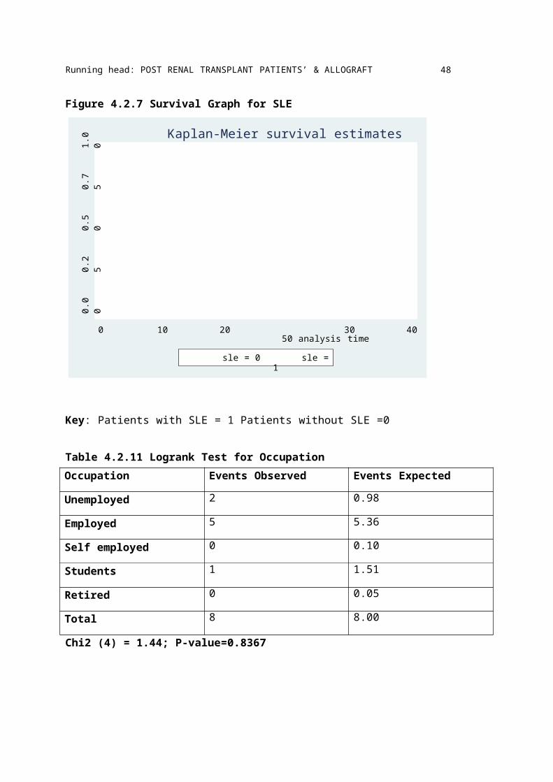
Table 4.2.10 Logrank Test for Systemic Lupus Erythematosus........................................................... 47
Table 4.2.11 Logrank Test for Occupation ......................................................................................... 48
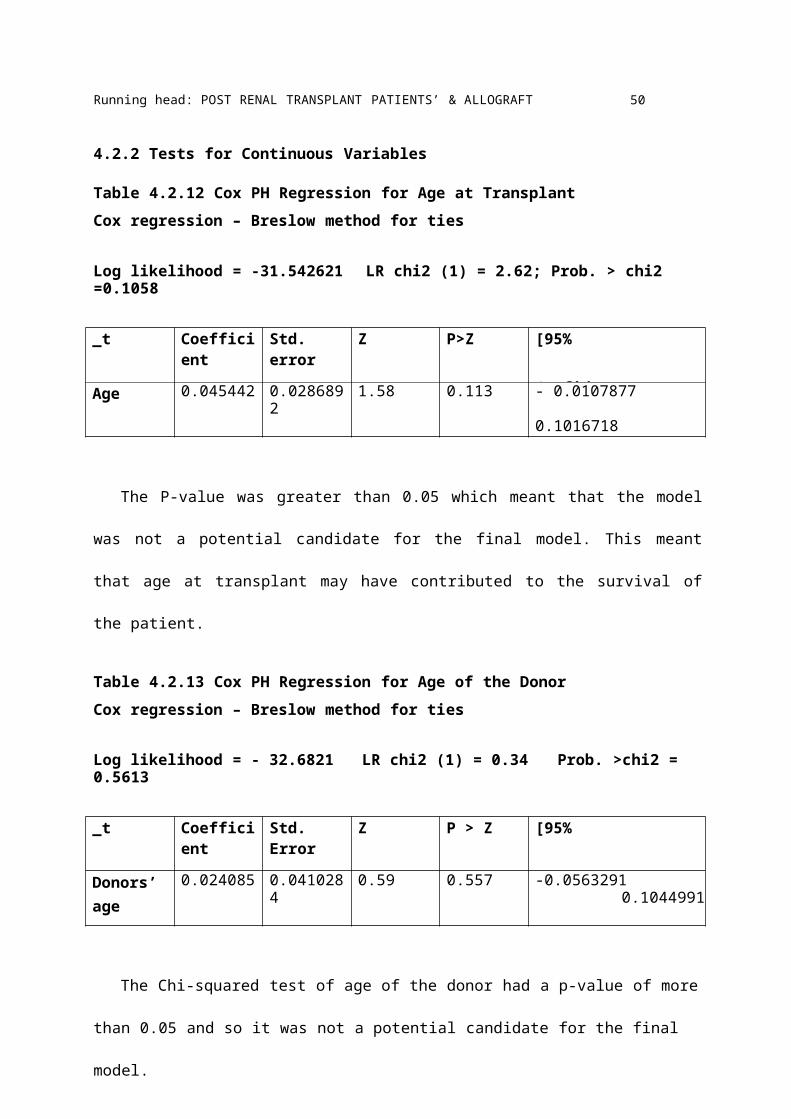
Table 4.2.12 Cox PH Regression for Age at Transplant...................................................................... 50
Table 4.2.13 Cox PH Regression for Age of the Donor ...................................................................... 50
Table 4.2.14 Cox regression – Breslow for ties .................................................................................. 51
Table 4.2.15 hazard ratio model ......................................................................................................... 52
Table 4.3.1 Renal Graft Survival Life Table....................................................................................... 53
Table 4.3.2 Renal Graft Survival Life Table....................................................................................... 56
Table 4.3.3 Logrank Test for Gender ................................................................................................. 58
Table 4.3.4 Logrank Test for Smoking Status..................................................................................... 59
Table 4.3.5 Logrank Test for Diabetes Mellitus.................................................................................. 60
Table 4.3.6 Logrank Test for Donor Relationship............................................................................... 62
Table 4.3.7 Logrank Test for HLA Mismatch..................................................................................... 64
Table 4.3.8 Logrank Test for SLE ...................................................................................................... 65
Table 4.3.9 Logrank Test for Occupation ........................................................................................... 66
Page 9
Running head: POST RENAL TRANSPLANT PATIENTS’ & ALLOGRAFT SURVIVAL ix
Table 4.3.10 Cox PH for Age at Transplant........................................................................................ 67
Table 4.3.11 Cox PH for Age of the Donor ........................................................................................ 67
Table 4.3.12 Cox PH model ............................................................................................................... 68
Table 4.3.13 Cox PHmodel With Hazard Ratio ................................................................................. 69
Page 10
Running head: POST RENAL TRANSPLANT PATIENTS’ & ALLOGRAFT SURVIVAL x
LIST OF FIGURES
Figure 4.1.1(a) Gender........................................................................................................................... 27
Figure 4.1.1 (b) Kidney Graft Status .................................................................................................. 28
Figure 4.1.1 (c) Patient Status ............................................................................................................ 28
Figure 4.1.1 (d) Smoking Status......................................................................................................... 29
Figure 4.1.1 (e) Status of Diabetes Mellitus ....................................................................................... 30
Figure 4.1.1 (f) Donor Relationships .................................................................................................. 31
Figure 4.1.1 (g) SLE Status................................................................................................................ 32
Figure 4.2.1 Survival Graph.............................................................................................................. 35
Figure 4.2.2 Kaplan-Meier survival Estimates for Gender .................................................................. 41
Figure 4.2.3 Kaplan Meier Survival Graph for smoking status.......................................................... 42
Figure 4.2.4 Kaplan Meier Survival Graph for Diabetes Mellitus ....................................................... 43
Figure 4.2.5 Survival Graph for Donor Relationship ......................................................................... 45
Figure 4.2.6 Survival Graph for HLA Missmatch .............................................................................. 47
Figure 4.2.7 Survival Graph for SLE.................................................................................................. 48
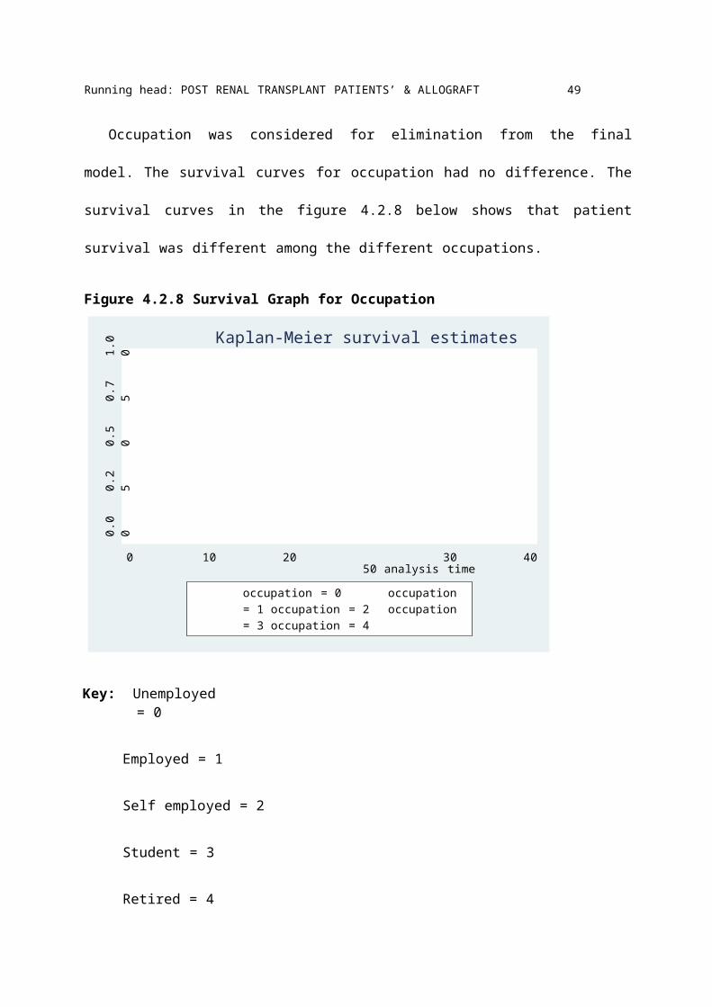
Figure 4.2.8 Survival Graph for Occupation....................................................................................... 49
Figure 4.3.1 Renal Graft Survival Graph ............................................................................................ 53
Figure 4.3.2 Renal Graft Survival Graph ............................................................................................ 58
Figure 4.3.3 Renal Graft Survival Graph for Gender .......................................................................... 59
Figure 4.3.4 Renal Graft Survival Graph for Smoking Status ............................................................. 60
Figure 4.3.5 Renal Graft Survival Graph for Diabetes Mellitus .......................................................... 61
Figure 4.3.6 Renal Graft Survival Graph for Donor Relationship ....................................................... 63
Figure 4.3.7 Renal Graft Survival Graph for HLA Mismatch ............................................................. 64
Figure 4.3.8 Renal Graft Survival Graph for SLE............................................................................... 65
Figure 4.3.9 Renal Graft Survival Graph for Occupation .................................................................... 66
Page 11
Running head: POST RENAL TRANSPLANT PATIENTS’ & ALLOGRAFT SURVIVAL xi
ACRONYMS
DWGF - Death with Graft Function
ESRD - End Stage Renal Disease
HLA - Human leukocyte antigen
KNH - Kenyatta National Hospital
SLE - Systemic Lupus Erythematosus
USA - United States of America
USRDS - US Renal Data System
WHO - World Health Organization
Page 12
Running head: POST RENAL TRANSPLANT PATIENTS’ & ALLOGRAFT SURVIVAL xii
DEFINITION OF TERMS
Age: the number of years the patient lived from birth to date of transplantation
Date of entry: the date when the transplant was done
Diabetes mellitus: Defined as a patient who has been diagnosed by a medical specialist to have
diabetes mellitus
Event: The event is the response variable i.e. patients death or kidney allograft failure
Gender: This is a qualitative measure of whether the patient is male of female
Graft survival: Time from transplant to graft failure (the time a kidney graft remains patent),
censoring for death with a functioning graft and grafts still functioning at time of analysis
Hypertension: Defined as the patient having a blood pressure of above 140/90 mmHg during the
period after transplantation of the allograft
Patient survival: Time from transplant to the time the patient experiences event of interest
(death)
Rejection: Allograft rejection will be considered to have taken place if the patient went back to
hemodialysis or undergoes another transplant
Smoking status: This is a qualitative measure of whether the patient has been smoking or not
during the period of the study
Time to event: The variable measures the duration to the event defined by the status variable;
Page 13
Running head: POST RENAL TRANSPLANT PATIENTS’ & ALLOGRAFT SURVIVAL xiii
a) The time taken until there is rejection of the kidney
b) The time taken by the patient from time of transplant to experiencing the
event death
The time of enrollment: This will be the month of transplant. Time will be measured in months.
Page 14
Running head: POST RENAL TRANSPLANT PATIENTS’ & ALLOGRAFT SURVIVAL 2
ABSTRACT
Renal transplantation has become the treatment of choice for most patients with end stage renal
disease (ESRD). Marked improvements in early graft survival and long-term graft function have
made kidney transplantation a more cost-effective alternative to dialysis.
This study was aimed at determining the patient and renal allograft survivals and identifying the
factors impacting on survival following kidney transplantation at Kenyatta National Hospital.
94 kidney transplant recipients who underwent renal transplant at Kenyatta National Hospital
from January 2010 to February 2014 were considered for the study. Survival analysis was used
in the analysis to assess the role of explanatory factors in time to death of a patient and time to
rejection of a kidney allograft. Outcome measures studied were patient and graft survival. Graft
loss was defined by the need for permanent renal dialysis, repeat transplantation or death with a
functioning graft. Kaplan-Meier method was be used to determine patient and graft survivals.
Cox proportional hazard model was used to determine the factors affecting survival. The
patients’ survival for the first year was 88.7%, second year 88.7%, third year 88.7% and 82.6%
for the fourth year. The trend showed that the survival was the same for the first three years then
a drop on the fourth year. For the patients who survived the operation, their survival was 92.7%
for the first, second and third year post transplant. The fouth year survival was 85.7%. The renal
allograft survival was 92.01% for the first and the second year, and 83.01% for the third and
fourth year. The graft survival for those who survived the transplant was 97.36 for the first and
the second year and 88.02% for the third and fourth year.
The factors that significantly influenced survival of renal transplanted patients were presence of
diabetes mellitus (p-value- 0.032) and the level of antigens of the human leukocyte antigen
(HLA) mismatch (p-value<0.0001). Factors that significantly influenced allograft survival were
Page 15
Running head: POST RENAL TRANSPLANT PATIENTS’ & ALLOGRAFT SURVIVAL 3
presence of Systemic lupus erythematosus (SLE) (p- value =0.025) and employment (p-value
=<0.0001). The results of the study concurred with other studies done elsewhere. In conclusion,
the study established that the survival rates in Kenyatta national hospital were good.
Page 16
Running head: POST RENAL TRANSPLANT PATIENTS’ & ALLOGRAFT SURVIVAL 4
CHAPTER ONE: INTRODUCTION
1.1 Background
The function of healthy kidneys in the body is to remove excess fluid, minerals, and wastes
from the blood and regulate blood pressure. If the kidneys are damaged, they don't work
properly. Harmful wastes build up in the body and blood pressure may rise. The body may retain
excess fluid and not make enough red blood cells. This defines kidney failure. If the kidneys fail,
treatment is needed to replace the work normally done by the kidneys. Treatment options
available are dialysis or kidney transplant. Each treatment option has its benefits and drawbacks.
Some changes in lifestyle need to be made after choosing any of the treatment options, including
eating and planning daily activities. But with the help of healthcare providers, family, and
friends, most people with kidney failure can lead full productive and active lives.
According to Naicker (2009), several studies have demonstrated a high incidence of chronic
kidney disease among black Americans. Unfortunately, lack of functioning registries in most of
Sub-Saharan Africa has resulted in a lack of reliable statistics. There is a general impression that
it is at least three to four times more frequent than in more developed countries; uremia
accounted for 1.0% - 1.5% of total annual deaths among Egyptians, both in the pre-dialysis era
and for two decades after (Naicker, 2009). The figures are comparable with those of other
countries of similar social economical standards.
Chronic kidney disease affects mainly young adults aged 20–50 years in sub-Saharan Africa
and is primarily due to hypertension and glomerular diseases. In the developed countries chronic
kidney disease presents in middle-aged and elderly patients and is predominantly due to diabetes
mellitus and hypertension (Arogundade & Barsoum 2008).
Page 17
Running head: POST RENAL TRANSPLANT PATIENTS’ & ALLOGRAFT SURVIVAL 5
The availability of renal replacement therapy in much of the Sub-Saharan Africa is limited
because of their high costs. Lack of available therapy is responsible for high rate of morbidity
and mortality. In 2004, renal replacement therapy was accessed by approximately 1.8 million
people worldwide. Five percent of the dialysis population was from Sub-Saharan Africa
(Grassman, Gioberge, Moeller, & Brown 2005).
There are more than one million Kenyans who suffer from kidney disease. There are less
than 100 working dialysis machines in the country (Singh 2012). Most of the patients in Kenya
with end-stage kidney failure either do not have access to a dialysis clinic or they cannot afford
to go to the very few available dialysis clinics (which are less than 10) since they are very
expensive (Singh 2012). The main causes of kidney disease in Kenya are mainly hypertension
and diabetes. Kenya also suffers from acute shortage of kidney specialists with one nephrologists
catering for a 100,000 people (Singh 2012). There is urgent need to train more kidney specialists
and renal nurses to cater for the increasing number of patients in the country.
According to the latest WHO data published in April 2011, Kidney Disease Deaths in Kenya
reached 2,912 or 0.92% of total deaths. The age adjusted Death Rate is 19.59 per 100,000 of
population ranks Kenya at position seventy seven (77) in the world.
Transplantation is limited by cost, donor shortages, and lack of a brain-death law in most of
sub-Saharan Africa (Naicker, 2009). Renal transplantation has become the treatment of choice
for most patients with end stage renal disease (ESRD). Marked improvements in early graft
survival and long-term graft function have made kidney transplantation a more cost-effective
alternative to dialysis (Collins & Kulkarni 2013). According to Collins & Kulkarni (2013),
studies show that renal transplantation prolongs patient lifespan when compared with dialysis.
Increasingly, patients on dialysis are being referred for transplant evaluation, which has resulted
Page 18
Running head: POST RENAL TRANSPLANT PATIENTS’ & ALLOGRAFT SURVIVAL 6
in burgeoning waitlists and increased waiting times for patients in need of kidney transplants. As
at 2013, more than 82,000 patients are waiting for kidney transplants in the United States.
1.2 Problem StatementThere is an increase in the number of patients suffering from chronic kidney failure in
Kenya. More than one million Kenyans suffer from kidney disease. Most of the patients in
Kenya with end-stage kidney failure either do not have access to a dialysis clinic or they cannot
afford to go to the very few available dialysis clinics (which are less than 10) since they are very
expensive (Singh 2012). The world health organization (WHO) (2011) reports the age adjusted
Death Rate in Kenya for kidney disease as 19.59 per 100,000 of population. The availability of
renal replacement therapy in much of the Sub-Saharan Africa is limited because of their high
costs. Lack of available therapy is responsible for high rate of morbidity and mortality
(Grassman et. al. 2005).
Renal transplantation has become the treatment of choice for most patients with end stage
renal disease (ESRD). KNH performs approximately four renal transplants per month.
Transplantation is limited by cost, donor shortages, and lack of a brain-death law in most of sub-
Saharan Africa (Naicker, 2009). Most patients in Kenya prefer hemodialysis because it is
economical in short term. Patients undergoing hemodialysis at KNH are dialyzed once a week
due to the patient machine ratio. Studies show that in the long term renal transplant is cheaper
and convenient compared to hemodialysis. Although long term survival following renal
transplantation remains below that of general population, it is much superior to that experienced
by patients undergoing dialysis. Lack of understanding of factors that influence the survival of
the kidney graft and transplant patients may lead a high rejection and death rate.
Page 19
Running head: POST RENAL TRANSPLANT PATIENTS’ & ALLOGRAFT SURVIVAL 7
1.3 Study JustificationThe number of patients undergoing hemodialysis can be reduced if the uptake for renal
transplant is improved. This can also reduce the patient machine ratio and will lead to better
survival of the patients. KNH is the only public hospital offering renal transplant services in
Kenya and there is no research done on patient and kidney allograft survival at the Renal Unit.
The results will also provide information to success of renal transplant and the factors that affect
renal survival. If the results show a high survival rate, the study will be used to improve the
uptake of renal transplantation in Kenya. If the results of the study show low survival rate, it will
be used to formulate policies to improve the service and survival.
1.4 Objectives of the StudyAim of this study is to determine the patient and renal-allograft survival and to identify
factors that may affect survival at Kenyatta National Hospital (KNH). The specific objectives
are:
i. To determine renal transplant patient and renal allograft survival rates using survival
analysis
ii. To identify risk factors that influence survival of renal kidney transplantees using Cox
regression model
iii. To identify the risk factors the contribute to renal allograft survival using Cox regression
model
1.5 Research QuestionWhat were the post renal transplant patients’ and allograft survival rates at Kenyatta
National Hospital Renal Unit between the year starting January 2010 to February 2014?
Page 20
Running head: POST RENAL TRANSPLANT PATIENTS’ & ALLOGRAFT SURVIVAL 8
CHAPTER TWO: LITERATURE REVIEW
2:1 IntroductionThis chapter presents a review of available literature that is pertinent to the study. The
review is divided into three main sections. The first section presents literature on renal transplant.
The second section review literature and studies on survival of post renal transplant patients. The
third section appraises studies on renal allograft survival.
2.2 Renal transplant
When a patient gets chronic kidney failure or end stage kidney disease, there are three
treatment options available: hemodialysis, peritoneal dialysis and kidney transplant. Without
long-term dialysis or a kidney transplant, the disease would prove to be fatal. A successful
kidney transplant provides a better quality of life compared to the other options. It offers greater
freedom and is often associated with increased energy levels and a less restricted diet. The source
of transplantation kidney can be a living donor or a deceased (non-living/ cadaver) donor. The
living donors can be related or unrelated to the patient. Cadaver organ comes from brain dead
people who have willed their kidneys before their death. All donors are carefully screened and
matched so that the recipient has maximum chances of a successful transplant.
The kidney transplant recipient is given immunosuppressant drugs to prevent the body’s
immune system from rejecting the new kidney. The transplanted kidney may function
immediately or may take a few weeks to function normally. The recipient is more prone to
infections due to the suppression of the body immunity. There is risk of rejection of the new
kidney as the body considers it to be a foreign object. It may occur soon after transplantation, or
several months or years after the procedure has taken place.
Page 21
Running head: POST RENAL TRANSPLANT PATIENTS’ & ALLOGRAFT SURVIVAL 9
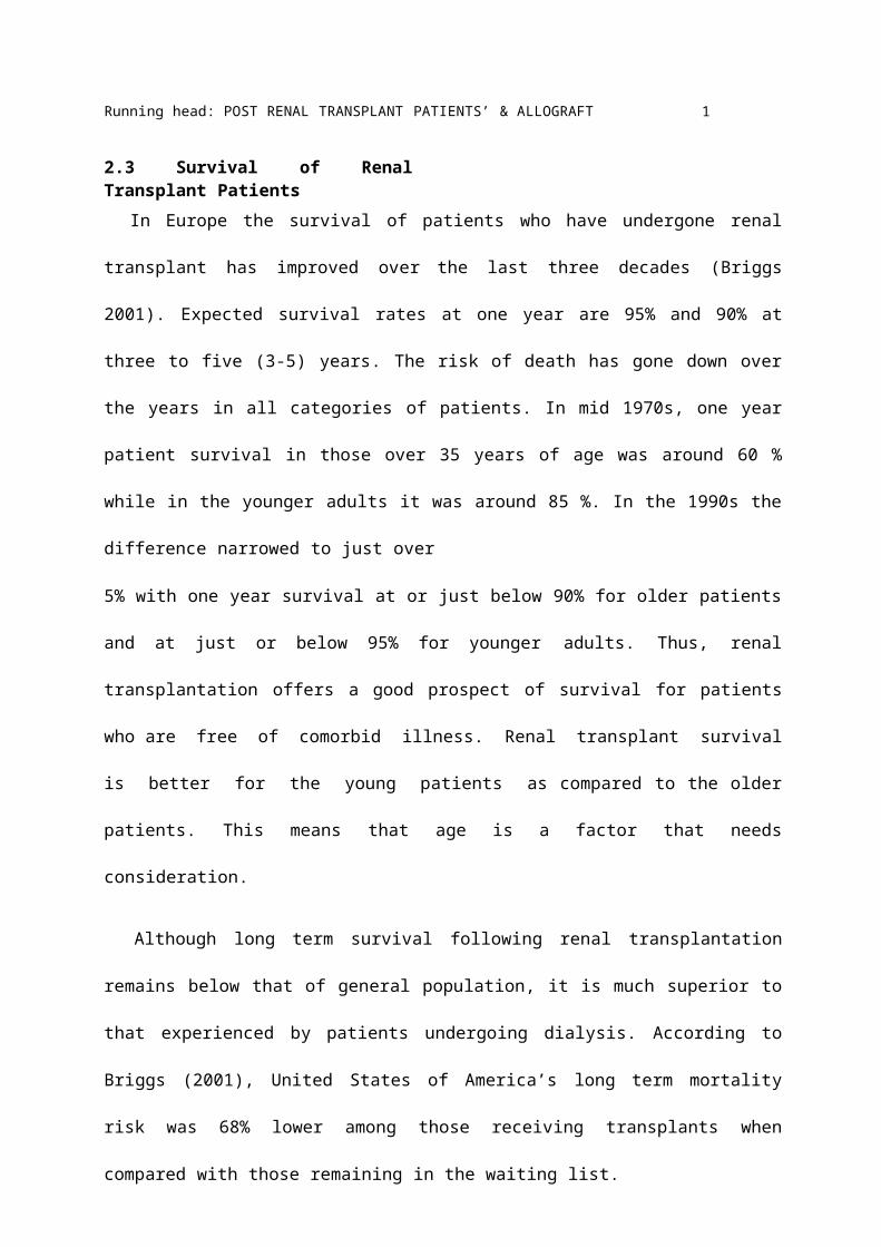
2.3 Survival of Renal Transplant PatientsIn Europe the survival of patients who have undergone renal transplant has improved over
the last three decades (Briggs 2001). Expected survival rates at one year are 95% and 90% at
three to five (3-5) years. The risk of death has gone down over the years in all categories of
patients. In mid 1970s, one year patient survival in those over 35 years of age was around 60 %
while in the younger adults it was around 85 %. In the 1990s the difference narrowed to just over
5% with one year survival at or just below 90% for older patients and at just or below 95% for
younger adults. Thus, renal transplantation offers a good prospect of survival for patients who
are free of comorbid illness. Renal transplant survival is better for the young patients as
compared to the older patients. This means that age is a factor that needs consideration.
Although long term survival following renal transplantation remains below that of general
population, it is much superior to that experienced by patients undergoing dialysis. According to
Briggs (2001), United States of America’s long term mortality risk was 68% lower among those
receiving transplants when compared with those remaining in the waiting list.
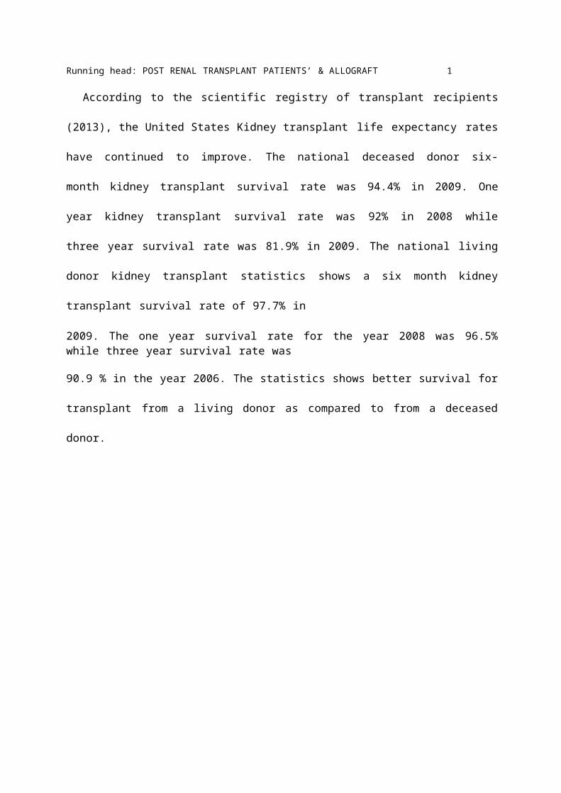
According to the scientific registry of transplant recipients (2013), the United States Kidney
transplant life expectancy rates have continued to improve. The national deceased donor six-
month kidney transplant survival rate was 94.4% in 2009. One year kidney transplant survival
rate was 92% in 2008 while three year survival rate was 81.9% in 2009. The national living
donor kidney transplant statistics shows a six month kidney transplant survival rate of 97.7% in
2009. The one year survival rate for the year 2008 was 96.5% while three year survival rate was
90.9 % in the year 2006. The statistics shows better survival for transplant from a living donor as
compared to from a deceased donor.
Page 22
Running head: POST RENAL TRANSPLANT PATIENTS’ & ALLOGRAFT SURVIVAL 10
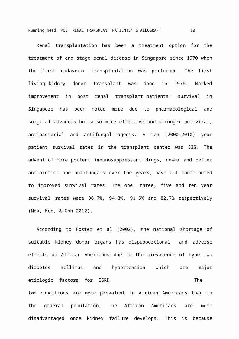
Renal transplantation has been a treatment option for the treatment of end stage renal disease
in Singapore since 1970 when the first cadaveric transplantation was performed. The first living
kidney donor transplant was done in 1976. Marked improvement in post renal transplant
patients’ survival in Singapore has been noted more due to pharmacological and surgical
advances but also more effective and stronger antiviral, antibacterial and antifungal agents. A ten
(2000-2010) year patient survival rates in the transplant center was 83%. The advent of more
portent immunosuppressant drugs, newer and better antibiotics and antifungals over the years,
have all contributed to improved survival rates. The one, three, five and ten year survival rates
were 96.7%, 94.8%, 91.5% and 82.7% respectively (Mok, Kee, & Goh 2012).
According to Foster et al (2002), the national shortage of suitable kidney donor organs has
disproportional and adverse effects on African Americans due to the prevalence of type two
diabetes mellitus and hypertension which are major etiologic factors for ESRD. The two
conditions are more prevalent in African Americans than in the general population. The African
Americans are more disadvantaged once kidney failure develops. This is because this patient
cohort has longer median waiting times on the renal transplant list and they have higher rates of
acute rejection.
As the immunosuppressive agents used to prevent acute rejection and the surgical techniques
have improved, so have the graft and patient survival rates. Studies have shown improved life
expectancy for patients who have undergone renal transplantation as opposed to patients who
have remained on dialysis. After two years of functioning, a living donor renal transplant is less
costly than maintaining the patient on hemodialysis. The quality of life of patients who have
undergone successful renal transplants is superior to that of those on dialysis (Foster et al. 2002).
Page 23
Running head: POST RENAL TRANSPLANT PATIENTS’ & ALLOGRAFT SURVIVAL 11
2.4 Renal Allograft SurvivalGraft survival is defined as time from transplant to graft failure, censoring for death with a
functioning graft and grafts still functioning at time of analysis.
In a retrospective study of 589 recipients of first deceased-donor allografts, mortality was
significantly increased patients with primary non-function compared to those with less severe
graft dysfunction (45 v/s 20% at years); however there were no significant difference in survival
among patients with delayed graft function versus immediate graft function (Tapiawala et. al.
2010). Death can occur while the graft is functioning or after kidney allograft failure. Death with
graft function (DWGF) has been reported to occur in 10 to 30% of patients. In an analysis of the
US Renal Data System (USRDS) by Ojo et al. (2000), 86,502 patients were studied, 18,482 of
whom died during a 10-yr period (7040 (38%) with graft function). Survival at 1, 5, and 10 yr
was 97, 91, and 86%, respectively. The median time from transplantation to death with function
was twenty three months.
According to Ojo et al. (2000) patients with a functioning graft have a high long term
survival. Although death with graft function is the major cause of graft loss, the risk has declined
substantially since 1990. Cardiovascular disease was the predominant reported cause of DWGF.
Other causes vary by post-transplant time period. Furthermore, the transplant operation, graft
loss, return to dialysis, and repeat transplantation are associated with variable time-dependent
mortality risks that may not be fully accounted for when overall post-transplant patient survival
is studied. The results of the observational study showed a marked and significant improvement
over time in the survival of renal transplant recipients with functioning grafts.
Singapore witnessed marked improvements in graft survival over a ten year period starting
from year 2000 to 2010 due to pharmacological and surgical advances (Mok et al 2012). The
Page 24
Running head: POST RENAL TRANSPLANT PATIENTS’ & ALLOGRAFT SURVIVAL 12
number of patients who received deceased donor transplantation in the 2000s compared to the
1980s had also increased following amendments to the Human Organ Transplant Act. In this
study the overall 10 year graft survival rate was 69.4%. The excellent overall graft survival was
helped by government subsidies for immunosuppressant drugs, which contributed to increased
patient compliance with medications. All patients in Singapore have lifelong follow up in a
tertiary hospital with a nephrologist. This could be another factor which contributed to good long
term outcomes. The results of the study also showed that live donors kidney transplants have
better short and long-term survival rates compared to deceased donor kidney transplants (Mok et
al 2012). Terasaki &, Ozawa (2004) have shown that ant-HLA antibodies, especially those that
develop post transplant, are an important cause of decreased long term graft survival.
Treatment of ESRD in South Africa has been an important public health issue (Rayner
2003). Prevalence of ESRD in South Africa as estimated by data from Europe and USA is 790
and 1400 per million populations respectively. The prevalence figures from the USA indicate a
marked increase of chronic renal failure in the African American population approximately
fourfold greater than the Caucasians American population. The South African figures are likely
to approximately exceed the US data. The Southern Africa dialysis and transplantation registry
estimate that only 99 cases per million populations receive treatment. Transplantation is cost
effective in the long term, offers the chance of full rehabilitation and can be offered to a greater
number of patients provided that there is sufficient supply of organs. The results of
transplantation are not properly documented. Most studies have originated from Europe or USA.
The Southern Africa Dialysis and Transplantation Registry have documented dialysis and
transplant outcomes in South Africa, but the last reliable report was issued in 1994. There is
Page 25
Running head: POST RENAL TRANSPLANT PATIENTS’ & ALLOGRAFT SURVIVAL 13
currently no central data collection system that tracks long-term survival rates for all the
transplant recipients in South Africa.
According to Arend et al (1997); Briggs (2001) some of the negative determinants of patient
survival are suggested to be; older age of recipients; male gender, presence of diabetes,
hypertension and cigarette smoking
Page 26
Running head: POST RENAL TRANSPLANT PATIENTS’ & ALLOGRAFT SURVIVAL 14
CHAPTER THREE: METHODOLOGY
3.1 Introduction
This chapter presents the statistical techniques used to analyze data. It also describes the key
aspects of survival models used in the study.
3.2 Study Area DescriptionThis study was conducted at the Kenyatta National Hospital (KNH) Renal Unit records
department. KNH is a major teaching and national referral hospitals in Kenya, East and Central
Africa. It was established in the year 1901 and became a corporate in 1987. It has a bed capacity
of 1800 patients. It is situated in Dagoretti constituency, Nairobi County, about 3 km from the
city centre, off Ngong Road on Hospital road and borders Mbagathi way to the south. The renal
Unit is situated on the first floor of the old hospital wing, opposite Critical Care Unit.
Approximately one hundred and fifty (150) patients undergo hemodialysis every week. Renal
transplantation is performed once a week. The unit also offers peritoneal dialysis.
3.3 Sampling
There was no sampling since the number of patients who underwent transplant during the
period was ninety four (94). The whole population was included in the study. The whole
population was eligible for the study. Initially the population was thought to be one hundred and
seven but on close scrutiny we found out that there was one who was done on 2009 and twelve in
2014.
Page 27
Running head: POST RENAL TRANSPLANT PATIENTS’ & ALLOGRAFT SURVIVAL 15
3.4 Data Collection
Data collection was undertaken by trained staff that looked at the patients’ files and
collected the required information. The trained staff was the registered nurse who has specialized
in renal nursing and co-ordinates renal transplantation in the unit. The role of the research
assistant was to collect data using a prepared check list. The data was entered in a database to
facilitate editing, coding and classification before analysis. The computer in which the data was
stored had a pass word of which not everybody could assess the data.
3.5 Ethical Consideration
Authority to conduct the study was sought from the Kenyatta National Hospital/ University
of Nairobi Ethical and Research committee. Permission was also sought from the head of
department renal unit Kenyatta National Hospital and the Head of medical records department.
Privacy and confidentiality was maintained by ensuring the information gathered was not
communicated to anyone, but was used for this study only. Patients’ names were not included in
the information as we used the patients’ identification number. No risks were subjected to the
patient. There may not be a direct benefit to the study population but the study may be useful in
terms of policy formulation. Raw data collected will be kept under key and lock for a period of
five years then destroyed by burning. Dissemination for the study results will be done through
the Head of Department (HOD) Kenyatta National Hospital research department and the HOD
Renal unit.
Page 28
Running head: POST RENAL TRANSPLANT PATIENTS’ & ALLOGRAFT SURVIVAL 16
3.6 Analytical Methods (Data Analysis and Methods)
3.6.1 Survival Analysis
Survival analysis models factors that influence the time to an event. Ordinary least squares
regression methods fall short because the time to event is typically not normally distributed, and
the model cannot handle censoring, very common in survival data, without modification.
Nonparametric methods provide simple and quick looks at the survival experience, and the Cox
proportional hazards regression model remains the dominant analysis method.
3.6.2 Distribution of Time to Event
In analyzing survival data we estimated the underlying true distribution (either parametric or
non parametric), then we were able to estimate other measures of interest such as measures of
location (central tendencies) of the survival times.
3.6.3 Using the Kaplan-Meier Method to Estimate Survival Curve
Kaplan-Meier estimate is one of the best options to be used to measure the fraction of
subjects living for a certain amount of time after treatment. In clinical trials or community trials,
the effect of an intervention is assessed by measuring the number of subjects survived or saved
after that intervention over a period of time. The time starting from a defined point to the
occurrence of a given event, for example death is called as survival time and the analysis of
group data as survival analysis. This can be affected by subjects under study that are
uncooperative and refused to be remained in the study or when some of the subjects may not
experience the event or death before the end of the study, although they would have experienced
or died if observation continued, or we lose touch with them midway in the study. We label these
situations as censored observations. The Kaplan-Meier estimate is the simplest way of
Page 29
Running head: POST RENAL TRANSPLANT PATIENTS’ & ALLOGRAFT SURVIVAL 17
computing the survival over time in spite of all these difficulties associated with subjects or
situations. The survival curve can be created assuming various situations. It involves computing
of probabilities of occurrence of event at a certain point of time and multiplying these successive
probabilities by any earlier computed probabilities to get the final estimate. This can be
calculated for two groups of subjects and also their statistical difference in the survivals.
In survival analysis there are two functions that are dependent on time and are of a particular
interest. These functions are the survival function S (t) and the hazard function h (t). Survival
function is defined as the probability of surviving to time t. The hazard function is the
conditional probability of dying at time t having survived to that time. Kaplan-Meier method was
used to estimate the survival curve without the assumption of the underlying probability
distribution. The method is based on the fact that the probability of surviving k or more time
periods from joining the study is a product of the observed survival rates for each period.
S (k) =P1*…*Pk (3.1)*P2
Here P1 is the proportion surviving the first period; P2 is the proportion surviving beyond the
second period having survived up to the second period as a condition and so on. The proportion
surviving period j conditional on having survived up to period j is;
Pi nj djnj (3.2)
Where nj is the number alive at the beginning of the period and dj is the number of deaths within
the period.
Page 30
Running head: POST RENAL TRANSPLANT PATIENTS’ & ALLOGRAFT SURVIVAL 18
3.6.3.1 The Hazard and Survival FunctionsLet T be a random variable representing the waiting time until the occurrence of the event.
The random variable is non-negative. One of the events of interest is rejection of allograft and
the other is death due to renal causes or renal complications. The survival time is the waiting
time.
The survival functionWith the assumption that T is a continuous random variable with probability density
function (p.d.f) f (t) and cumulative function (c.d.f) F (t) = Pr [T t ], giving the probability that
the probability that the event has occurred during time t.
S (t) = Pr [T>t] =1- F (t) = (3.3)
This gives the probability that the event of interest did not occur by duration t. In our case it
means the probability the allograft was not rejected by duration t.
The Hazard FunctionDistribution of T is also given by the hazard function. Hazard function h(t) is the
instantaneous rate of occurrence of the event;
h(t) = dt lim 0Pr( t T t dt / T t )
dt(3.4)
The numerator of the above equation is the conditional probability that the event will occur in the
interval (t, t+dt) given that the event has not occurred before. The denominator represents the
interval width. With this we obtain a rate of event occurrence per unit time. Taking the limit
down to zero, we obtain an instantaneous rate of occurrence.
Page 31
The conditional probability in the numerator may be written as the ratio of the joint
probability that T is in the interval (t, t + dt) and T >t. The former may be written as f (t)dt for
small dt, while the later is S (t) by definition. Dividing by dt and passing to the limit gives the
following;
h(t) =f (t )S (t )
(3.5)
Where f(t) is the density function and S(t) is the survival function Collet (2003).
A closely related function to the hazard function is the cumulative hazard function H(t);
H(t) = - ln(S(t)) (3.6)
3.6.4 Comparing the survival of two groups (Log-rank test)
The log-rank test is used to compare two or more groups of survival times. It tests the null
hypothesis that the groups are from the same population. The log-rank test compares the
observed number of events in each group with the corresponding expected numbers for each.
Survival times from two groups can be obtained by plotting the corresponding estimates of the
two survival functions on the same axes. The summary statistics which will be obtained across
the two groups can be compared. Log-rank test is used to compare the statistics. It is used to test
the null hypothesis. The null hypothesis of no difference can be obtained between groups can be
expressed by stating that the median survival of the two groups are equal.
Page 32
Running head: POST RENAL TRANSPLANT PATIENTS’ & ALLOGRAFT SURVIVAL 20
3.6.4.1 Procedure for calculating the log-rank test two groups A & B (Machin, Campbell
&Walters 2013)
i. The total number of events observed in groups A& B are OA and OB
ii. Under the null hypothesis, the expected number of events receiving treatment A at
time ti is eAi= (dinAi)/ni (3.7)
ti = ordered survival time
eAi = Expected number of events in A
di = number of events at ti
nAi = number at risk in A
iii. the expected number of events should not be calculated beyond the last event
iv. the total number of events expected on A, assuming the null hypothesis of no
difference between treatments, is EA=∑eAi (3.8)
v. The number expected on B is EB=∑di-EA. (3.9)
vi. Calculate X2 Log-rank = (O A E A ) 2 + (OB
E A
EB )2EB
(3.10)
vii. This has a X2 distribution with degree of freedom df=1 as two groups are being
compared
3.6.5 Multivariate Survival Analysis
3.6.5.1 Cox Proportional – Hazards ModelProportional Hazards Regression using a partial maximum likelihood function to estimate
the covariate parameters in the presence of censored time to failure data (Cox, 1972) has become
widely used for conducting survival analysis. The Cox model is based on a modeling approach to
Page 33
the analysis of survival data. The purpose of the model is to simultaneously explore the effects of
several variables on survival.
It deals with the analysis of data which have the following characteristics:
1. The dependent variable is the waiting time until the occurrence of a well defined event
2. The observations are censored (some units the event of interest has not occurred at time
of data analysis)
3. There are predictor variables whose effect on the waiting time needs to be assessed.
According to Wilson (2013), Model adequacy focuses on overall fitness, validity of the
linearity assumption, inclusion (or exclusion) of a correct (or an incorrect) covariate, and
identification of outlier and highly-influential observations. Due to the presence of censored data
and the use of the partial maximum likelihood function, diagnostics to assess these elements in
proportional hazards regression compared to most modeling exercises can be slightly more
complicated.
The proportional hazards (PH) regression model has two kinds of assumptions, that when
satisfied ordinarily allow one to rely on the statistical inferences and predictions the model
yields. The first assumption is that the time independence of the covariates in the hazard
function, that is, the ratio of the hazard function for two individuals with different regression
covariates, does not vary with time, which is also known as the PH assumption. The second
assumption is that the relationship between log cumulative hazard and a covariate is linear.
3.6.5.2 Fitting the Cox Proportional Hazard ModelA Cox regression analysis yields an equation for the hazard as a function of several
explanatory variables. This entails obtaining parameter estimates for the unknown beta (β)
Page 34
coefficients. The baseline hazard h0 (t) may also be estimated. These two components were
estimated separately by first estimating the beta (β) using the Maximum Likelihood Estimator
methods and then h0 (t) non-parametrically. According to Cox (1972), one can obtain consistent
and highly efficient estimators of betas (β) by maximizing a partial likelihood independently of
h0 (t).
The multivariable Cox model links the hazard to an individual i at time t, hi (t) to a baseline
hazard h0 (t) by;
log [hi (t)]= log[h0(t)] + β1x1+ β2x2+…+ βkxk (3.11)
Where x1, x2…xk are covariates associated with individual i. The baseline log hazard, log [h0 (t)],
serves as a reference point, and can be thought of as the intercept, α, of a multiple regression
equation.
The coefficients in a Cox regression relate to hazard; a positive coefficient indicates a worse
prognosis and a negative coefficient indicates a protective effect of the variable with which it is
associated. The interpretation of the hazards ratio depends upon the measurement scale of the
predictor variable in question.
3.6.5.3 Time-dependent and fixed covariatesIn prospective studies, when individuals are followed over time, the values of covariates
may change with time. Covariates can thus be divided into fixed and time-dependent. A
covariate is time dependent if the difference between its values for two different subjects changes
with time; e.g. serum cholesterol. A covariate is fixed if its values cannot change with time, e.g.
sex or race. Lifestyle factors and physiological measurements such as blood pressure are usually
time-dependent. Cumulative exposures such as smoking are also time-dependent but are often
Page 35
forced into an imprecise dichotomy, i.e. "exposed" vs. "not-exposed" instead of the more
meaningful "time of exposure". There are no hard and fast rules about the handling of time
dependent covariates.
3.6.5.4 Model analysis and deviance
A test of the overall statistical significance of the model is given under the "model analysis"
option. Here the likelihood chi-square statistic is calculated by comparing the deviance (- 2 * log
likelihood) of the model, with all of the covariates you have specified, against the model with all
covariates dropped. The individual contribution of covariates to the model can be assessed from
the significance test given with each coefficient in the main output; this assumes a reasonably
large sample size. Deviance is minus twice the log of the likelihood ratio for models fitted by
maximum likelihood (Cox 1972).The value of adding a parameter to a Cox model is tested by
subtracting the deviance of the model with the new parameter from the deviance of the model
without the new parameter, the difference is then tested against a chi-square distribution with
degrees of freedom equal to the difference between the degrees of freedom of the old and new
models. The model analysis option tests the model you specify against a model with only one
parameter, the intercept; this tests the combined value of the specified predictors/covariates in
the model.
Page 36
CHAPTER FOUR: RESULTS AND ANALYSIS
4.0 IntroductionThis chapter describes the analysis of data and the findings of the study.
4.0.1 Study DesignThe study design was a retrospective cohort of patients who underwent renal transplant for
the four year period between January 2010 and February 2014. Patient’s demographic data,
history of investigations, Comorbidity, and health history during the transplant period were
obtained.
4.0.2 Study population.
Target population in a study is the whole population in which the researcher has interest and
to which the researcher will postulate the findings. The study population comprised of all chronic
renal failure patients who underwent kidney transplant for the four year period between January
2010 and February 2014.
4.0.3. Inclusion and Exclusion Criteria
4.0.3.1 Inclusion Criteria
All patients who underwent renal transplant at Kenyatta National Hospital renal Unit
between year January 2010 and February 2014 were included in the study.
4.0.3.2 Exclusion Criteria
All patients who underwent renal transplant outside Kenyatta Hospital and were attending
clinic at the Renal Unit Clinic were excluded from the study.
Page 37
4.0.4 Key variables in survival analysis are;
4.0.4.1 Time to event: The variable measures the duration to the event defined by the status
variable. In this case it is the time taken for the patient to reject a kidney allograft and also the
time taken by the patient from time of transplant to death. The time of enrollment was the month
of transplant. Time was measured in months.
4.0.4.2 Status variable (outcome variables): Also called the event or censoring variable. It
is the response or the dependent variable in Cox regression. In this study event variables are the
rejection of the allograft and death of the patient. Graft survival is defined as time from
transplant to graft failure, censoring for death with a functioning graft and grafts still functioning
at time of analysis. The rejection was considered to have taken place if the patient went back to
hemodialysis or undergoes another transplant. Those who rejected the allograft were considered
to experience the event in the case of allograft survival while others were censored. Those who
died with a working allograft were said to have survived in the case of allograft survival. Patients
who died due to kidney related causes and complications were said to have experienced the event
in the case of patient survival while others were censored. Events were coded as 1 and censored
as 0. The outcomes were obtained from the file using a check list whereby we read through the
file and charted all the outcomes.
4.0.4.3 Covariates: these are independent variables which were tested for their association
with the events of interest. Some covariates were tested for their association with time to
allograft rejection and patient’s death.
The following are required for survival analysis to be successful;
Page 38
Date of entry ( date of transplantation): the date when the transplant was done
Well defined scale of measurement: the scale of measurement was the number of months
since transplantation to the event or to exit.
Well defined event of interest (allograft rejection or death due to kidney complications)
Definition:
Age – the number of years the patient lived from birth to date of transplantation.
Gender- the qualitative measure of whether the patient is male of female
Smoking status:- the qualitative measure of whether the patient was smoking or
not during the period after transplantation
Hypertension: - this was defined as the patient having a blood pressure of above
140/90 mmHg during the period after transplantation of the allograft.
Diabetes mellitus: - this was defined as a patient who had been diagnosed by a
medical specialist to have diabetes mellitus and was on treatment for the same.
4.1 Baseline Enrollment Characteristics
A total of ninety four (94) clients were enrolled into the study. The study included all the
patients who underwent renal transplant at Kenyatta National Hospital between the months of
February 2010 to the month of February 2014. 70.2% were male while 29.8% were female. All
the subjects who were transplanted at Kenyatta National Hospital were hypertensive. Among
those enrolled in the study, twenty six (26) were diabetic & two (2) smokers. Eight (8) kidney
allografts failed post transplant while eighty six (86) survived. Twelve (12) patients died while
eighty two (82) survived. All the kidney donors were life donors. They were all relatives to the
patients. Majority of the donors were female. Only two patients had Systemic Lupus
Erythematosus (SLE).
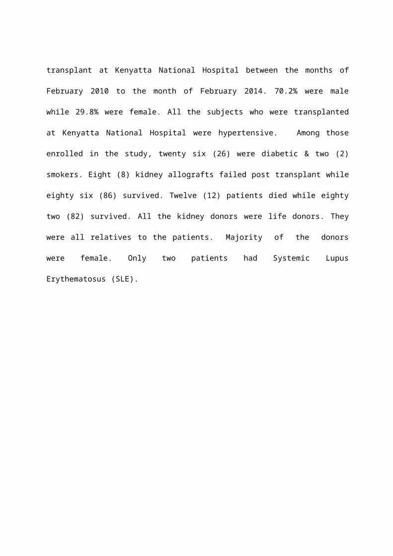
Page 39
Out of 94 subjects 66 were male while 28 were female. Figure 4.1.1 (a) illustrates composition of
gender.
Figure 4.1.1(a) Gender
28, 30%
male
female
66, 70%
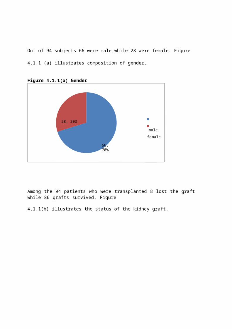
Among the 94 patients who were transplanted 8 lost the graft while 86 grafts survived. Figure
4.1.1(b) illustrates the status of the kidney graft.
Page 40
Figure 4.1.1 (b) Kidney Graft Status
8, 9%
86, 91%
failed
survived
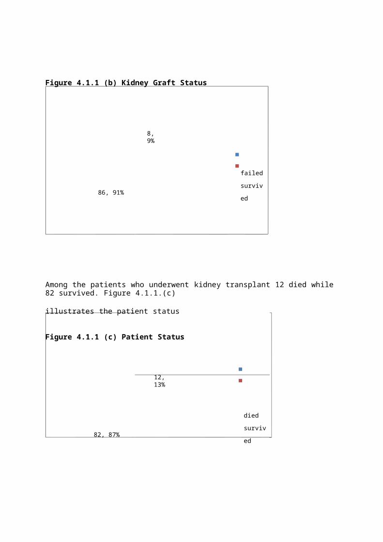
Among the patients who underwent kidney transplant 12 died while 82 survived. Figure 4.1.1.(c)
illustrates the patient status
Figure 4.1.1 (c) Patient Status
12, 13%
82, 87%
died
survived
Page 41
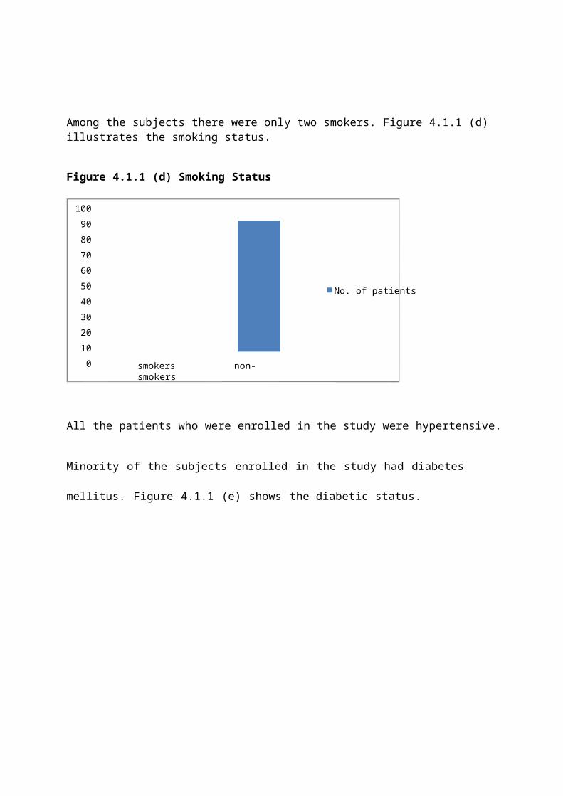
Among the subjects there were only two smokers. Figure 4.1.1 (d) illustrates the smoking status.
Figure 4.1.1 (d) Smoking Status
100908070605040302010
0
smokers non-smokers
No. of patients
All the patients who were enrolled in the study were hypertensive.
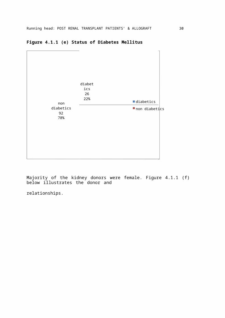
Minority of the subjects enrolled in the study had diabetes mellitus. Figure 4.1.1 (e) shows the
diabetic status.
Page 42
Running head: POST RENAL TRANSPLANT PATIENTS’ & ALLOGRAFT SURVIVAL 30
Figure 4.1.1 (e) Status of Diabetes Mellitus
non diabetics92
78%
diabetics26
22%
diabetics
non diabetics
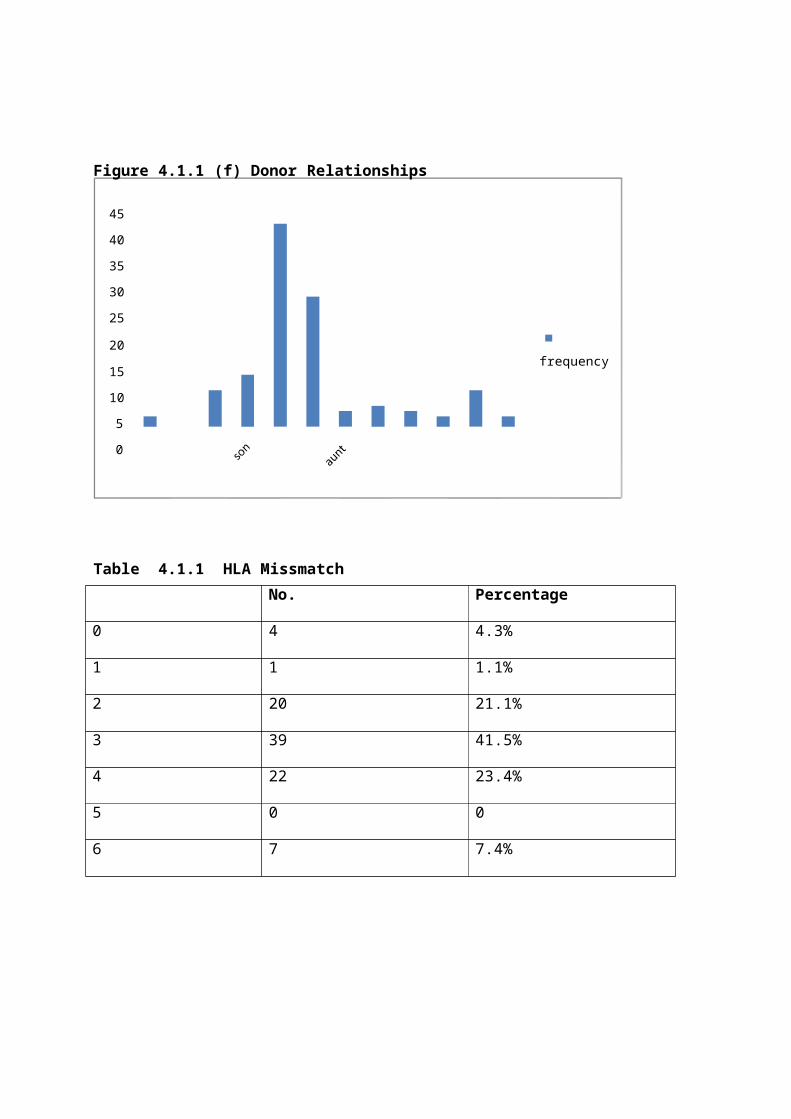
Majority of the kidney donors were female. Figure 4.1.1 (f) below illustrates the donor and
relationships.
Page 43
Figure 4.1.1 (f) Donor Relationships
45
40
35
30
25
20frequency
15
10
5
0
Table 4.1.1 HLA MissmatchNo. Percentage
0 4 4.3%
1 1 1.1%
2 20 21.1%
3 39 41.5%
4 22 23.4%
5 0 0
6 7 7.4%
Page 44
%
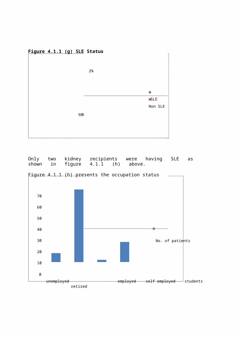
Figure 4.1.1 (g) SLE Status
2%
SLE
Non SLE
98
Only two kidney recipients were having SLE as shown in figure 4.1.1 (h) above.
Figure 4.1.1 (h) presents the occupation status
70
60
50
40
30 No. of patients
20
10
0
unemployed employed self employed students retired
Page 45
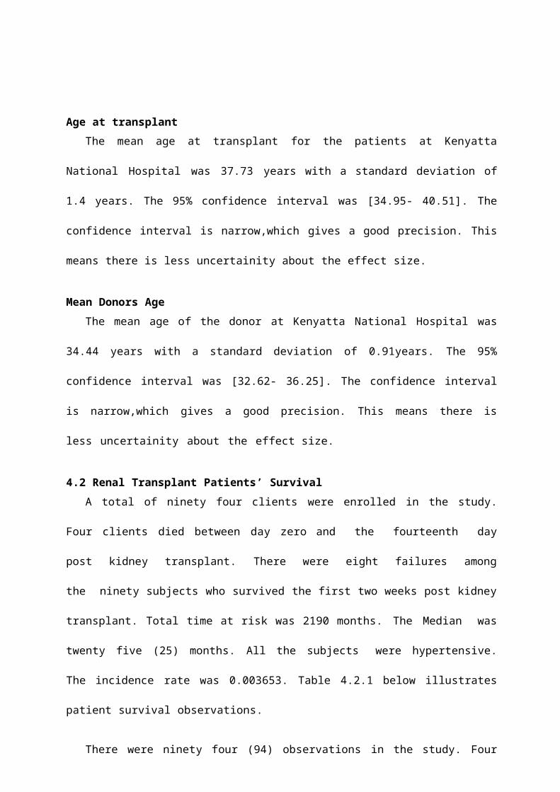
Age at transplantThe mean age at transplant for the patients at Kenyatta National Hospital was 37.73 years
with a standard deviation of 1.4 years. The 95% confidence interval was [34.95- 40.51]. The
confidence interval is narrow,which gives a good precision. This means there is less uncertainity
about the effect size.
Mean Donors AgeThe mean age of the donor at Kenyatta National Hospital was 34.44 years with a standard
deviation of 0.91years. The 95% confidence interval was [32.62- 36.25]. The confidence interval
is narrow,which gives a good precision. This means there is less uncertainity about the effect
size.
4.2 Renal Transplant Patients’ SurvivalA total of ninety four clients were enrolled in the study. Four clients died between day zero
and the fourteenth day post kidney transplant. There were eight failures among the ninety
subjects who survived the first two weeks post kidney transplant. Total time at risk was 2190
months. The Median was twenty five (25) months. All the subjects were hypertensive. The
incidence rate was 0.003653. Table 4.2.1 below illustrates patient survival observations.
There were ninety four (94) observations in the study. Four (4) of the subjects died on or
before they entered the study. This is to mean that they died on the day of transplant or within the
first two weeks post transplant. These are the patients who did not leave the hospital alive post
transplant. Ninety subjects remained in the study. Among the ninety subjects there were eight (8)
failures. By failure we mean deaths. The total analysis time at time zero (t=0) at risk was 2190
months. The last observed exit was at forty nine (49) months.
Page 46
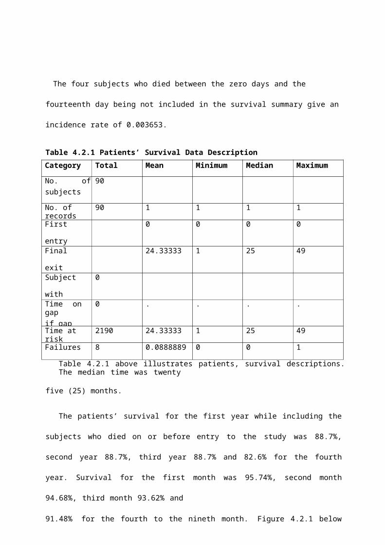
The four subjects who died between the zero days and the fourteenth day being not included in
the survival summary give an incidence rate of 0.003653.
Table 4.2.1 Patients’ Survival Data DescriptionCategory Total Mean Minimum Median Maximum
No. ofsubjects
90
No. of records 90 1 1 1 1
First entrytime
0 0 0 0
Final exittime
24.33333 1 25 49
Subject withgap
0
Time on gapif gap
0 . . . .
Time at risk 2190 24.33333 1 25 49
Failures 8 0.0888889 0 0 1
Table 4.2.1 above illustrates patients, survival descriptions. The median time was twenty
five (25) months.
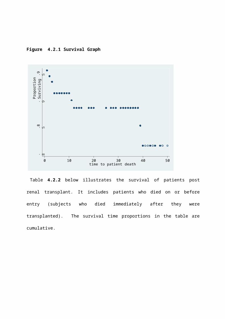
The patients’ survival for the first year while including the subjects who died on or before
entry to the study was 88.7%, second year 88.7%, third year 88.7% and 82.6% for the fourth
year. Survival for the first month was 95.74%, second month 94.68%, third month 93.62% and
91.48% for the fourth to the nineth month. Figure 4.2.1 below illustrates the Kaplan-Meier
survival graph for the patients survival post renal transplant.
Page 47
Pro
porti
on S
urvi
ving
.8.8
5.9
.95
Figure 4.2.1 Survival Graph
0 10 20 30 40 50 time to patient death
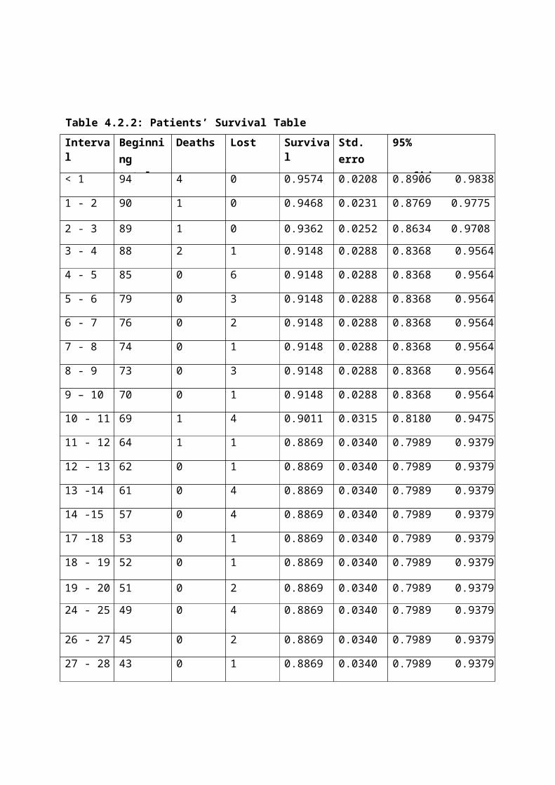
Table 4.2.2 below illustrates the survival of patients post renal transplant. It includes patients
who died on or before entry (subjects who died immediately after they were transplanted). The
survival time proportions in the table are cumulative.
Page 48
Table 4.2.2: Patients’ Survival Table
Interval Beginning total
Deaths Lost Survival Std. error
95% confidence interval
< 1 94 4 0 0.9574 0.0208 0.8906 0.9838
1 - 2 90 1 0 0.9468 0.0231 0.8769 0.9775
2 - 3 89 1 0 0.9362 0.0252 0.8634 0.9708
3 - 4 88 2 1 0.9148 0.0288 0.8368 0.9564
4 - 5 85 0 6 0.9148 0.0288 0.8368 0.9564
5 - 6 79 0 3 0.9148 0.0288 0.8368 0.9564
6 - 7 76 0 2 0.9148 0.0288 0.8368 0.9564
7 - 8 74 0 1 0.9148 0.0288 0.8368 0.9564
8 - 9 73 0 3 0.9148 0.0288 0.8368 0.9564
9 – 10 70 0 1 0.9148 0.0288 0.8368 0.9564
10 - 11 69 1 4 0.9011 0.0315 0.8180 0.9475
11 - 12 64 1 1 0.8869 0.0340 0.7989 0.9379
12 - 13 62 0 1 0.8869 0.0340 0.7989 0.9379
13 -14 61 0 4 0.8869 0.0340 0.7989 0.9379
14 -15 57 0 4 0.8869 0.0340 0.7989 0.9379
17 -18 53 0 1 0.8869 0.0340 0.7989 0.9379
18 - 19 52 0 1 0.8869 0.0340 0.7989 0.9379
19 - 20 51 0 2 0.8869 0.0340 0.7989 0.9379
24 - 25 49 0 4 0.8869 0.0340 0.7989 0.9379
26 - 27 45 0 2 0.8869 0.0340 0.7989 0.9379
27 - 28 43 0 1 0.8869 0.0340 0.7989 0.9379
Page 49
28 -29 42 0 1 0.8869 0.0340 0.7989 0.9379
30 - 31 41 0 3 0.8869 0.0340 0.7989 0.9379
31 - 32 38 0 2 0.8869 0.0340 0.7989 0.9379
32 - 33 36 0 3 0.8869 0.0340 0.7989 0.9379
33 - 34 33 0 1 0.8869 0.0340 0.7989 0.9379
34 - 35 32 0 1 0.8869 0.0340 0.7989 0.9379
35 - 36 31 0 2 0.8869 0.0340 0.7989 0.9379
36 - 37 29 0 1 0.8869 0.0340 0.7989 0.9379
37 - 38 28 0 1 0.8869 0.0340 0.7989 0.9379
38 - 39 27 1 1 0.8535 0.0464 0.7333 0.9223
39 - 40 25 1 5 0.8155 0.0578 0.6684 0.9019
40 - 41 19 0 2 0.8155 0.0578 0.6684 0.9019
41 - 42 17 0 2 0.8155 0.0578 0.6684 0.9019
42 - 43 15 0 2 0.8155 0.0578 0.6684 0.9019
43 - 44 13 0 1 0.8155 0.0578 0.6684 0.9019
44 - 45 12 0 1 0.8155 0.0578 0.6684 0.9019
46 - 47 11 0 1 0.8155 0.0578 0.6684 0.9019
47 - 48 10 0 9 0.8155 0.0578 0.6684 0.9019
49 - 50 1 0 1 0.8155 0.0578 0.6684 0.9019
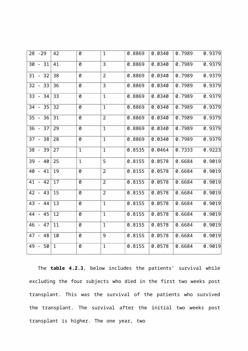
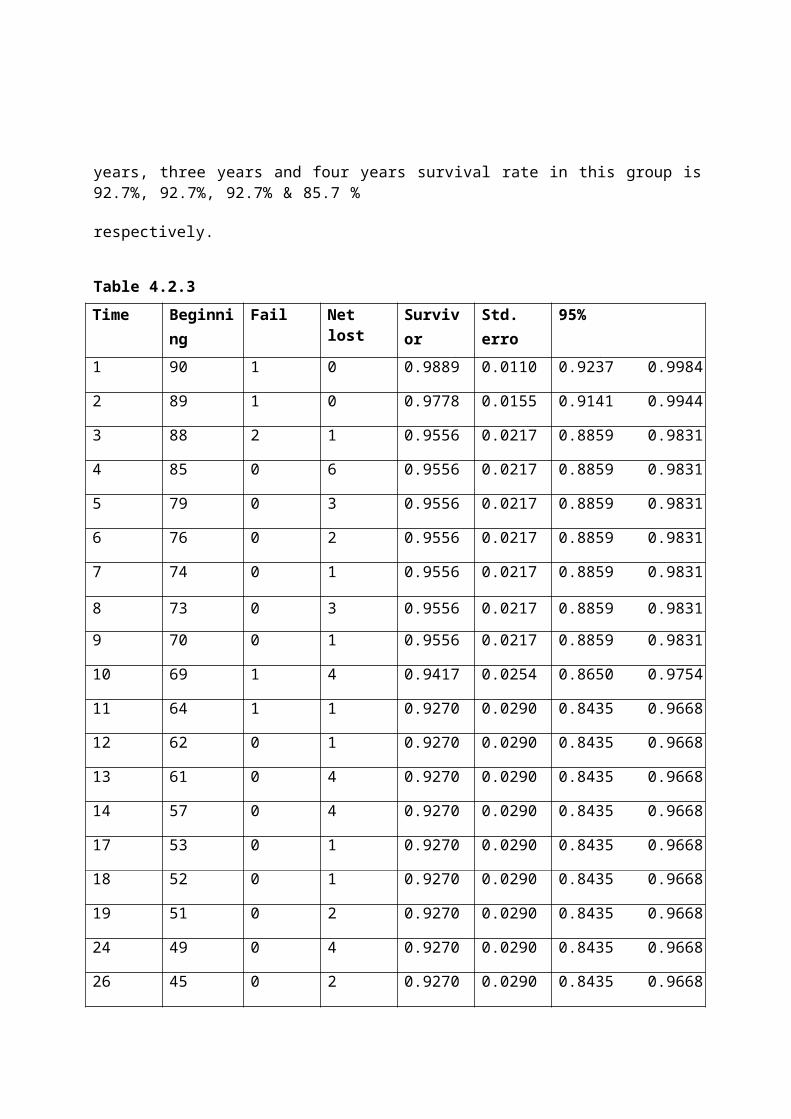
The table 4.2.3, below includes the patients’ survival while excluding the four subjects who
died in the first two weeks post transplant. This was the survival of the patients who survived the
transplant. The survival after the initial two weeks post transplant is higher. The one year, two
Page 50
years, three years and four years survival rate in this group is 92.7%, 92.7%, 92.7% & 85.7 %
respectively.
Table 4.2.3Time Beginning
totalFail Net lost Survivor
functionStd. error
95% Confidence interval
1 90 1 0 0.9889 0.0110 0.9237 0.9984
2 89 1 0 0.9778 0.0155 0.9141 0.9944
3 88 2 1 0.9556 0.0217 0.8859 0.9831
4 85 0 6 0.9556 0.0217 0.8859 0.9831
5 79 0 3 0.9556 0.0217 0.8859 0.9831
6 76 0 2 0.9556 0.0217 0.8859 0.9831
7 74 0 1 0.9556 0.0217 0.8859 0.9831
8 73 0 3 0.9556 0.0217 0.8859 0.9831
9 70 0 1 0.9556 0.0217 0.8859 0.9831
10 69 1 4 0.9417 0.0254 0.8650 0.9754
11 64 1 1 0.9270 0.0290 0.8435 0.9668
12 62 0 1 0.9270 0.0290 0.8435 0.9668
13 61 0 4 0.9270 0.0290 0.8435 0.9668
14 57 0 4 0.9270 0.0290 0.8435 0.9668
17 53 0 1 0.9270 0.0290 0.8435 0.9668
18 52 0 1 0.9270 0.0290 0.8435 0.9668
19 51 0 2 0.9270 0.0290 0.8435 0.9668
24 49 0 4 0.9270 0.0290 0.8435 0.9668
26 45 0 2 0.9270 0.0290 0.8435 0.9668
Page 51
27 43 0 1 0.9270 0.0290 0.8435 0.9668
28 42 0 1 0.9270 0.0290 0.8435 0.9668
30 41 0 3 0.9270 0.0290 0.8435 0.9668
31 38 0 2 0.9270 0.0290 0.8435 0.9668
32 36 0 3 0.9270 0.0290 0.8435 0.9668
33 33 0 1 0.9270 0.0290 0.8435 0.9668
34 32 0 1 0.9270 0.0290 0.8435 0.9668
35 31 0 2 0.9270 0.0290 0.8435 0.9668
36 29 0 1 0.9270 0.0290 0.8435 0.9668
37 28 0 1 0.9270 0.0290 0.8435 0.9668
38 27 1 1 0.8927 0.0438 0.7675 0.9524
39 25 1 5 0.8570 0.0547 0.7078 0.9336
40 19 0 2 0.8570 0.0547 0.7078 0.9336
41 17 0 2 0.8570 0.0547 0.7078 0.9336
42 15 0 2 0.8570 0.0547 0.7078 0.9336
43 13 0 1 0.8570 0.0547 0.7078 0.9336
44 12 0 1 0.8570 0.0547 0.7078 0.9336
46 11 0 1 0.8570 0.0547 0.7078 0.9336
47 10 0 9 0.8570 0.0547 0.7078 0.9336
49 1 0 1 0.8570 0.0547 0.7078 0.9336
Page 52
Running head: POST RENAL TRANSPLANT PATIENTS’ & ALLOGRAFT SURVIVAL 40
Table 4.2.4 Failure Rates as Per GenderTotal observations included in the analysis = 90 subjects
Gender Died Estimated Rate 95% confidence intervals
Lower Upper
Female 3 0.0041265 0.0013309 0.0127946
Male 5 0.0034176 0.0014225 0.0082110
Five (5) male patients died after they survived the first two weeks post-transplant, while
three (3) female patients died at the same period. The failure rate for the female was higher than
that for the male patients.
4.2.1 Non Parametric Test for Categorical VariablesKaplan-Meier survival curve was used to analyze survival at fixed time points and then
comparisons were made of the patients survival times exceeding the period. The periods are in
months. Logrank test was used to compare the survival times of the two groups.
Table 4.2.5 Logrank Test for GenderGender Events observed Events expected
Female 3 2.74
Male 5 5.26
Total 8 8.00
Chi2 (1) = 0.04; p-value = 0.8455
Page 53
0.00
0.25
0.50
0.75
1.00
Running head: POST RENAL TRANSPLANT PATIENTS’ & ALLOGRAFT SURVIVAL 41
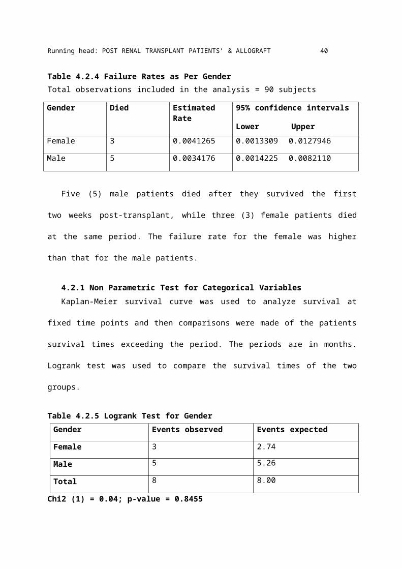
Figure 4.2.2 Kaplan-Meier survival Estimates for Gender
Kaplan-Meier survival estimates
0 10 20 30 4050 analysis time
gender = 0 gender = 1
Key: analysis time = time to patients’ death.
Gender: female = 0; Male = 1
The test P-value is higher than 0.05. This meant that gender was not to be considered as a
predictor in the final model. Through the Logrank test we considered to eliminate gender. The
Kaplan-Meier survival curve suggests that there was no difference in terms of survival for both
gender.
Page 54
0.00
0.25
0.50
0.75
1.00
Running head: POST RENAL TRANSPLANT PATIENTS’ & ALLOGRAFT SURVIVAL 42
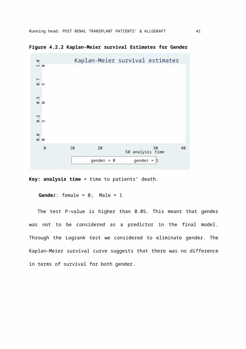
Table 4.2.6: Logrank Test for Smoking StatusSmoking status Events observed Events expected
Non-smoker 8 7.88
Smoker 0 0.12
total 8 8.00
Chi2 (1) = 0.12, p-value = 0.7254
Since the P-value was above 0.05, we considered eliminating smoking status from the final
model. The number of the smokers was only two against ninety two non-smokers. This may have
affected the significance of the results.
Figure 4.2.3 Kaplan Meier Survival Graph for smoking status
Kaplan-Meier survival estimates
0 10 20 30 4050 analysis time
smokingstatus = 0 smokingstatus = 1
Key: Non-Smoker = 0; Smoker =1; Analysis Time = time to patient’s death
Page 55
0.00
0.25
0.50
0.75
1.00
Running head: POST RENAL TRANSPLANT PATIENTS’ & ALLOGRAFT SURVIVAL 43
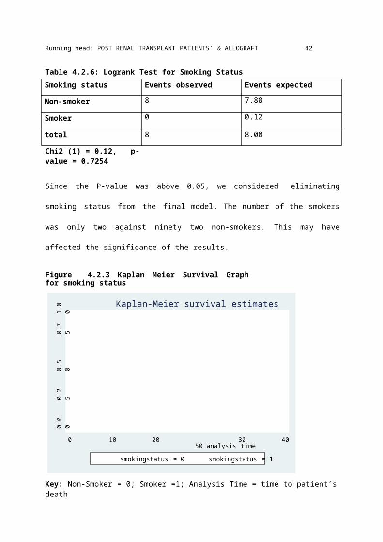
Table 4.2.7 Logrank Test for Diabetes MellitusDiabetes Mellitus Events observed Events Expected
Non- Diabetic 3 5.73
Diabetic 5 2.27
Total 8 8.00
Chi2 (1) = 4.60, p-value = 0.032
Diabetes mellitus was considered for inclusion in the final model because of the P-value of
0.0320. Diabetic patients had a lower probability of surviving compared to non diabetic patients.
This meant that diabetic status affected survival of the patients post transplant.
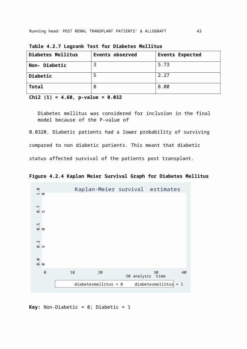
Figure 4.2.4 Kaplan Meier Survival Graph for Diabetes Mellitus
Kaplan-Meier survival estimates
0 10 20 30 4050 analysis time
diabetesmellitus = 0 diabetesmellitus = 1
Key: Non-Diabetic = 0; Diabetic = 1
Page 56
Running head: POST RENAL TRANSPLANT PATIENTS’ & ALLOGRAFT SURVIVAL 44
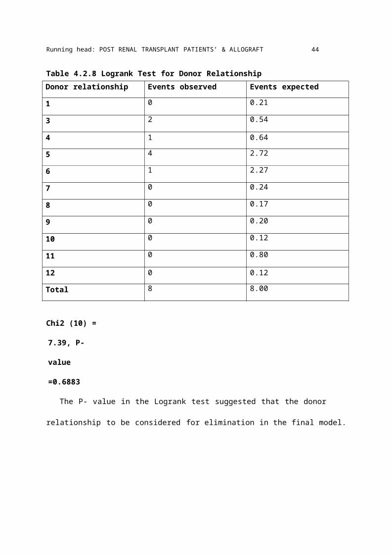
Table 4.2.8 Logrank Test for Donor RelationshipDonor relationship Events observed Events expected
1 0 0.21
3 2 0.54
4 1 0.64
5 4 2.72
6 1 2.27
7 0 0.24
8 0 0.17
9 0 0.20
10 0 0.12
11 0 0.80
12 0 0.12
Total 8 8.00
Chi2 (10) = 7.39,
P-value =0.6883
The P- value in the Logrank test suggested that the donor relationship to be considered for
elimination in the final model.
Page 57
0.00
0.
25
0.50
0.
75
1.00
Running head: POST RENAL TRANSPLANT PATIENTS’ & ALLOGRAFT SURVIVAL 45
Figure 4.2.5 Survival Graph for Donor Relationship
Kaplan-Meier survival estimates
0 10 20 30 4050 analysis time
donorrelationship = 1 donorrelationship = 3 donorrelationship = 4 donorrelationship = 5 donorrelationship = 6 donorrelationship = 7 donorrelationship = 8 donorrelationship = 9 donorrelationship = 10 donorrelationship = 11donorrelationship = 12
Key: Husband=1; Wife=2; Daughter = 3; Son = 4; Sister = 5; Brother = 6; Aunt = 7; Uncle =8;
Cousin =9; Nephew = 10; Mother =11; Father =12.
All the donors in the study were relatives to the patients. They were live donors. The Kaplan-
Meier survival curves shows that different donor relationships had a difference in survival of
patients post transplant.
Page 58
Running head: POST RENAL TRANSPLANT PATIENTS’ & ALLOGRAFT SURVIVAL 46
Table 4.2.9 Logrank Test for HLA MismatchHLA Mismatch Events Observed Events Expected
0 0 0.32
1 1 0.10
2 1 1.05
3 5 3.81
4 1 2.23
6 0 0.50
Total 8 8.00
Chi2 (5) = 10.27, P- value = 0.0681
The antigens of the human leukocyte antigen (HLA) system were considered for the model. The
HLA mismatch of zero (0) meant that there was perfect match. HLA mismatch played a role in
the survival of the patient depending on the level. Figure 4.2.6 below illustrates the Kaplan-
Meier survival curves for HLA mismatch.
Page 59
0.00
0.25
0.50
0.75
1.00
Running head: POST RENAL TRANSPLANT PATIENTS’ & ALLOGRAFT SURVIVAL 47
Figure 4.2.6 Survival Graph for HLA Missmatch
Kaplan-Meier survival estimates
0 10 20 30 4050 analysis time
hlamismatch = 0 hlamismatch = 1 hlamismatch = 2 hlamismatch = 3hlamismatch = 4 hlamismatch = 6
Table 4.2.10 Logrank Test for Systemic Lupus ErythematosusSLE Events Observed Events Expected
Non SLE patient 8 7.77
SLE patient 0 0.23
Total 8 8.00
Chi2 (1) = 0.23; P- value = 0.6278
SLE was considered for elimination from the final model. The survival curves were not different.
The number of patients who had SLE was few compared to those who did not have SLE.
Page 60
0.00
0.25
0.50
0.75
1.00
Running head: POST RENAL TRANSPLANT PATIENTS’ & ALLOGRAFT SURVIVAL 48
Figure 4.2.7 Survival Graph for SLE
Kaplan-Meier survival estimates
0 10 20 30 4050 analysis time
sle = 0 sle = 1
Key: Patients with SLE = 1 Patients without SLE =0
Table 4.2.11 Logrank Test for OccupationOccupation Events Observed Events Expected
Unemployed 2 0.98
Employed 5 5.36
Self employed 0 0.10
Students 1 1.51
Retired 0 0.05
Total 8 8.00
Chi2 (4) = 1.44; P-value=0.8367
Page 61
0.00
0.25
0.50
0.75
1.00
Running head: POST RENAL TRANSPLANT PATIENTS’ & ALLOGRAFT SURVIVAL 49
Occupation was considered for elimination from the final model. The survival curves for
occupation had no difference. The survival curves in the figure 4.2.8 below shows that patient
survival was different among the different occupations.
Figure 4.2.8 Survival Graph for Occupation
Kaplan-Meier survival estimates
0 10 20 30 4050 analysis time
occupation = 0 occupation = 1 occupation = 2 occupation = 3 occupation = 4
Key: Unemployed = 0
Employed = 1
Self employed = 2
Student = 3
Retired = 4
Page 62
Running head: POST RENAL TRANSPLANT PATIENTS’ & ALLOGRAFT SURVIVAL 50
4.2.2 Tests for Continuous Variables
Table 4.2.12 Cox PH Regression for Age at TransplantCox regression – Breslow method for ties
Log likelihood = -31.542621 LR chi2 (1) = 2.62; Prob. > chi2 =0.1058
_t Coefficient Std. error Z P>Z [95% Confidence interval
Age at transplant
0.045442 0.0286892 1.58 0.113 - 0.0107877 0.1016718
The P-value was greater than 0.05 which meant that the model was not a potential candidate
for the final model. This meant that age at transplant may have contributed to the survival of the
patient.
Table 4.2.13 Cox PH Regression for Age of the DonorCox regression – Breslow method for ties
Log likelihood = - 32.6821 LR chi2 (1) = 0.34 Prob. >chi2 = 0.5613
_t Coefficient Std. Error Z P > Z [95% Confidence interval]
Donors’age
0.024085 0.0410284 0.59 0.557 -0.0563291 0.1044991
The Chi-squared test of age of the donor had a p-value of more than 0.05 and so it was not a
potential candidate for the final model.
Page 63
Running head: POST RENAL TRANSPLANT PATIENTS’ & ALLOGRAFT SURVIVAL 51
Model BuildingFor the model building, we first considered the model which included all the predictors that
had a p-value of less than 0.2 - 0.25 in the univariate analyses. Categorical variables considered
were, diabetes mellitus, and HLA mismatch. The continuous variable considered was age at
transplant. The categorical predictor HLA mismatch has seven levels and therefore we included
this predictor using dummy variable with the group HLA mismatch =0 as the reference group.
Table 4.2.14 Cox regression – Breslow for tiesLog likelihood = -27.004323, LR Chi2 (6) = 11.69; Prob. > chi2 =0.0692
_t Coefficient Std. error Z P > Z [95% Confidence interval]
Age at transplant
0.0220069 0.0372266 0.59 0.554 -0.0509559 0.0949698
DiabetesMellitus
1.542578 0.9916366 1.56 0.120 -0.400994 3.48615
HLAmismatch
124.48769 . . . .
2 21.1603 1.545323 13.68 0.000 18.13152 24.18908
3 21.42517 1.288839 16.62 0.000 18.89909 23.95124
4 20.36073 1.584286 12.85 0.000 17.25559 23.461587
6 -21.37695 3.10e+09 -0.00 1.000 -6.08e+09 6.08e+09
The results were not statistically significant for age at transplant and diabetes mellitus. There
were significant results for HLA mismatch. As the level of mismatch increases the patient was
more likely to experience the event which was death.
Page 64
Running head: POST RENAL TRANSPLANT PATIENTS’ & ALLOGRAFT SURVIVAL 52
P< 0.05 shows there is statistical significance.
Table 4.2.15 hazard ratio modelLog likelihood = -27.004323, LR Chi2 (6) = 11.69; Prob. > chi2 =0.0692
_t Hazard ratio
Std. error Z P > Z [95% Confidence interval]
Age at transplant
1.022251 0.038055 0.59 0.554 0.9503205 1.099626
DiabetesMellitus
4.676632 4.637519 1.56 0.120 0.6696541 32.65997
HLAmismatch
14.31e+10 . . . .
2 1.55e+09 2.39e+09 13.68 0.000 7.49e+07 3.2e+10
3 2.02e+09 2.60e+09 16.62 0.000 1.61e+08 2.52e+10
4 6.96e+08 1.10e+09 12.85 0.000 3.12e+07 1.55e+10
6 5.20e-10 1.614521 -0.00 1.000 .
4.3 Renal Graft SurvivalA total of ninety four patients were done kidney transplant during the four years study
period. Eight subjects rejected their kidney immediately. By immediately we mean before two
weeks erupts after the transplant. This then left eighty six patients in the study. The total analysis
time was 2152 months. There were five failures of the patients who survived the first two
weeks. In total the failures were thirteen.
Page 65
Pro
porti
on S
urvi
ving
.8.8
5.9
.95
Running head: POST RENAL TRANSPLANT PATIENTS’ & ALLOGRAFT SURVIVAL 53
Figure 4.3.1 Renal Graft Survival GraphThe first and second year graft survival was 92.01%. the third and fourth year survival went
down to 83.01%.
0 10 20 30 40 50 time to graft death
Table 4.3.1 below illustrates the renal graft survival for all the ninety four subjects in the
study. Interval 0 -1 indicates that five kidneys were rejected while three patients were censored.
The survival times is in months.
Table 4.3.1 Renal Graft Survival Life TableInterval Beginning
totalDeaths Lost Survival Std.
error95% confidence interval
O - 1 94 5 3 0.9459 0.0235 0.8750 0.9771
1 - 2 86 0 1 0.9459 0.0235 0.8750 0.9771
3 - 4 85 0 1 0.9459 0.0235 0.8750 0.9771
Page 66
Running head: POST RENAL TRANSPLANT PATIENTS’ & ALLOGRAFT SURVIVAL 54
4 - 5 84 1 6 0.9343 0.0260 0.8594 0.9699
5 - 6 77 0 3 0.9343 0.0260 0.8594 0.9699
6 - 7 74 0 2 0.9343 0.0260 0.8594 0.9699
8 - 9 72 0 3 0.9343 0.0260 0.8594 0.9699
9 – 10 69 0 1 0.9343 0.0260 0.8594 0.9699
10 - 11 68 1 4 0.9201 0.0292 0.8389 0.9613
11 - 12 63 0 1 0.9201 0.0292 0.8389 0.9613
12 - 13 62 0 1 0.9201 0.0292 0.8389 0.9613
13 -14 61 0 4 0.9201 0.0292 0.8389 0.9613
14 -15 57 0 4 0.9201 0.0292 0.8389 0.9613
17 -18 53 0 1 0.9201 0.0292 0.8389 0.9613
18 - 19 52 0 1 0.9201 0.0292 0.8389 0.9613
19 - 20 51 0 2 0.9201 0.0292 0.8389 0.9613
24 - 25 49 0 4 0.9201 0.0292 0.8389 0.9613
26 - 27 45 0 2 0.9201 0.0292 0.8389 0.9613
27 - 28 43 0 1 0.9201 0.0292 0.8389 0.9613
28 -29 42 0 1 0.9201 0.0292 0.8389 0.9613
30 - 31 41 0 3 0.9201 0.0292 0.8389 0.9613
31 - 32 38 1 2 0.8952 0.0375 0.7926 0.9487
32 - 33 35 0 3 0.8952 0.0375 0.7926 0.9487
33 - 34 32 0 1 0.8952 0.0375 0.7926 0.9487
34 - 35 31 0 1 0.8952 0.0375 0.7926 0.9487
35 - 36 30 0 2 0.8952 0.0375 0.7926 0.9487
36 - 37 28 2 1 0.8301 0.0564 0.6836 0.9129
Page 67
Running head: POST RENAL TRANSPLANT PATIENTS’ & ALLOGRAFT SURVIVAL 55
37 - 38 25 0 1 0.8301 0.0564 0.6836 0.9129
38 - 39 24 0 1 0.8301 0.0564 0.6836 0.9129
39 - 40 23 0 5 0.8301 0.0564 0.6836 0.9129
40 - 41 18 0 2 0.8301 0.0564 0.6836 0.9129
41 - 42 16 0 2 0.8301 0.0564 0.6836 0.9129
42 - 43 14 0 1 0.8301 0.0564 0.6836 0.9129
43 - 44 13 0 1 0.8301 0.0564 0.6836 0.9129
44 - 45 12 0 1 0.8301 0.0564 0.6836 0.9129
46 - 47 11 0 1 0.8301 0.0564 0.6836 0.9129
47 - 48 10 0 9 0.8301 0.0564 0.6836 0.9129
49 - 50 1 0 1 0.8301 0.0564 0.6836 0.9129
Page 68
Running head: POST RENAL TRANSPLANT PATIENTS’ & ALLOGRAFT SURVIVAL 56
The life table below (table 4.3.2) excludes the eight subjects who lost their kidney allografts
between the zero day and fourteenth day post transplant.
Table 4.3.2 Renal Graft Survival Life TableTime Beginning
totalFail Net lost Survivor
functionStd. error
95% Confidence interval
1 86 0 1 1.000 . . .
3 85 0 1 1.000 . . .
4 84 1 6 0.9881 0.118 0.9185 0.9983
5 77 0 3 0.9881 0.118 0.9185 0.9983
6 74 0 2 0.9881 0.118 0.9185 0.9983
8 72 0 3 0.9881 0.118 0.9185 0.9983
9 69 0 1 0.9881 0.118 0.9185 0.9983
10 68 1 4 0.9736 0.185 0.8977 0.9934
11 63 0 1 0.9736 0.185 0.8977 0.9934
12 62 0 1 0.9736 0.185 0.8977 0.9934
13 61 0 4 0.9736 0.185 0.8977 0.9934
14 57 0 4 0.9736 0.185 0.8977 0.9934
17 53 0 1 0.9736 0.185 0.8977 0.9934
18 52 0 1 0.9736 0.185 0.8977 0.9934
19 51 0 2 0.9736 0.185 0.8977 0.9934
24 49 0 4 0.9736 0.185 0.8977 0.9934
26 45 0 2 0.9736 0.185 0.8977 0.9934
27 43 0 1 0.9736 0.185 0.8977 0.9934
28 42 0 1 0.9736 0.185 0.8977 0.9934
Page 69
Running head: POST RENAL TRANSPLANT PATIENTS’ & ALLOGRAFT SURVIVAL 57
30 41 0 3 0.9736 0.185 0.8977 0.9934
31 38 1 2 0.9479 0.0311 0.8371 0.9841
32 35 0 3 0.9479 0.0311 0.8371 0.9841
33 32 0 1 0.9479 0.0311 0.8371 0.9841
34 31 0 1 0.9479 0.0311 0.8371 0.9841
35 30 0 2 0.9479 0.0311 0.8371 0.9841
36 28 2 1 0.8802 0.0544 0.7191 0.9519
37 25 0 1 0.8802 0.0544 0.7191 0.9519
38 24 0 1 0.8802 0.0544 0.7191 0.9519
39 23 0 5 0.8802 0.0544 0.7191 0.9519
40 18 0 2 0.8802 0.0544 0.7191 0.9519
41 16 0 2 0.8802 0.0544 0.7191 0.9519
42 14 0 1 0.8802 0.0544 0.7191 0.9519
43 13 0 1 0.8802 0.0544 0.7191 0.9519
44 12 0 1 0.8802 0.0544 0.7191 0.9519
46 11 0 1 0.8802 0.0544 0.7191 0.9519
47 10 0 9 0.8802 0.0544 0.7191 0.9519
49 1 0 1 0.8802 0.0544 0.7191 0.9519
Page 70
0.00
0.25
0.50
0.75
1.00
Running head: POST RENAL TRANSPLANT PATIENTS’ & ALLOGRAFT SURVIVAL 58
Figure 4.3.2 Renal Graft Survival Graph
Kaplan-Meier survival estimate
0 10 20 30 4050 analysis time
Key: analysis time = time to rejection
Table 4.3.3 Logrank Test for GenderGender Events Observed Events Expected
Female 2 1.81
Male 3 3.19
Total 5 5.00
Chi2 (1) = 0.03; P-value = 0.8538
The p-value for the test is more 0.05, so it was considered for elimination from the final model.
The Kaplan-Meier survival curves were not different for either gender.
Page 71
0.00
0.25
0.50
0.75
1.00
Running head: POST RENAL TRANSPLANT PATIENTS’ & ALLOGRAFT SURVIVAL 59
Figure 4.3.3 Renal Graft Survival Graph for Gender
Kaplan-Meier survival estimates
0 10 20 30 4050 analysis time
gender = 0 gender = 1
Key: 0 = Female; 1=Male
Table 4.3.4 Logrank Test for Smoking Status
Smoking status Events Observed Events Expected
Non-smoker 5 4.96
Smoker 0 0.04
Total 5 5.00
Chi2 (1) = 0.04; P-value= 0.8428
Smoking status considered for elimination in the final model because the P-value is above 0.05.
Page 72
Running head: POST RENAL TRANSPLANT PATIENTS’ & ALLOGRAFT SURVIVAL 600.
000.
250.
500.
751.
00
Figure 4.3.4 Renal Graft Survival Graph for Smoking Status
Kaplan-Meier survival estimates
0 10 20 30 4050 analysis time
smokingstatus = 0 smokingstatus = 1
Key; Non-smoker = 0; Smoker = 1
Table 4.3.5 Logrank Test for Diabetes MellitusDiabetes mellitus Events Observed Events Expected
Non-diabetic 3 3.64
Diabetic 2 1.36
Total 5 5.00
Chi2 (1) = 0.42; P-value= 0.5162
Diabetes mellitus was considered for elimination.
Page 73
0.00
0.25
0.50
0.75
1.00
Running head: POST RENAL TRANSPLANT PATIENTS’ & ALLOGRAFT SURVIVAL 61
Figure 4.3.5 Renal Graft Survival Graph for Diabetes Mellitus
Kaplan-Meier survival estimates
0 10 20 30 4050 analysis time
diabetesmellitus = 0 diabetesmellitus = 1
Key; Non-Diabetic = 0; Diabetic = 1
There was no difference in the allograft survival for the diabetic and non diabetic patients in
the study.
Page 74
Running head: POST RENAL TRANSPLANT PATIENTS’ & ALLOGRAFT SURVIVAL 62
Table 4.3.6 Logrank Test for Donor RelationshipDonor relationships Events Observed Events Expected
Husband 0 0.12
Daughter 1 0.35
Son 0 0.31
Sister 1 1.73
Brother 1 1.50
Aunt 1 0.15
Uncle 0 0.08
Cousin 0 0.09
Nephew 0 0.04
Mother 1 0.59
Father 0 0.04
Total 5 5.00
Chi2 (10) = 7.69; P-value = 0.6594
Donor relationship was considered for elimination since the P-value was above 0.05.
Page 75
0.00
0.
25
0.50
0.
75
1.00
Running head: POST RENAL TRANSPLANT PATIENTS’ & ALLOGRAFT SURVIVAL 63
Figure 4.3.6 Renal Graft Survival Graph for Donor Relationship
Kaplan-Meier survival estimates
0 10 20 30 4050 analysis time
donorrelationship = 1 donorrelationship = 3 donorrelationship = 4 donorrelationship = 5 donorrelationship = 6 donorrelationship = 7 donorrelationship = 8 donorrelationship = 9 donorrelationship = 10 donorrelationship = 11donorrelationship = 12
Key = husband=1; wife=2; daughter = 3; son = 4; sister = 5; brother = 6; aunt = 7; uncle =8;
Cousin =9; nephew = 10; mother =11; father =12.
The Kaplan-Meier survival curves for the donor relationships showed no difference in
regard to allograft survival.
Page 76
0.00
0.25
0.50
0.75
1.00
Running head: POST RENAL TRANSPLANT PATIENTS’ & ALLOGRAFT SURVIVAL 64
Table 4.3.7 Logrank Test for HLA MismatchHLA Mismatch Events Observed Events Expected
0 0 0.16
1 0 0.03
2 2 0.51
3 1 2.37
4 2 1.75
6 0 0.17
Total 5 5.00
Chi2 (5) = 5.63; P-value=0.3438
The hla Mismatch was considered for elimination in the final model due to the P-value.
Figure 4.3.7 Renal Graft Survival Graph for HLA Mismatch
Kaplan-Meier survival estimates
0 10 20 30 4050 analysis time
hlamismatch = 0 hlamismatch = 1 hlamismatch = 2 hlamismatch = 3 hlamismatch = 4 hlamismatch = 6
Page 77
0.00
0.25
0.50
0.75
1.00
Running head: POST RENAL TRANSPLANT PATIENTS’ & ALLOGRAFT SURVIVAL 65
Table 4.3.8 Logrank Test for SLESLE Events Observed Events Expected
Non- SLE Patient 4 4.85
SLE Patient 1 0.15
Total 5 5.00
Chi2 (1) =5.02; P-value=0.0251
SLE was considered for the final model. The graft survival for those with SLE and those
without as shown by the Kaplan-Meier survival graph below was different. So SLE may have an
effect in the survival of the kidney allograft.
Figure 4.3.8 Renal Graft Survival Graph for SLE
Kaplan-Meier survival estimates
0 10 20 30 4050 analysis time
sle = 0 sle = 1
Key; SLE Patients = 1, Non SLE Patient = 0; analysis time = time in months
Page 78
0.00
0.25
0.50
0.75
1.00
Running head: POST RENAL TRANSPLANT PATIENTS’ & ALLOGRAFT SURVIVAL 66
Table 4.3.9 Logrank Test for OccupationOccupation Events Observed Events Expected
Unemployed 2 0.69
Employed 1 3.41
Self employed 1 0.04
Student 1 0.85
Retired 0 0.01
Total 5 5.00
Chi2 (4) = 28.52; Pr <0.0001
Occupation was considered for the final model. The survival of the graft for the employed
was better than for the rest.
Figure 4.3.9 Renal Graft Survival Graph for Occupation
Kaplan-Meier survival estimates
0 10 20 30 4050 analysis time
occupation = 0 occupation = 1 occupation = 2 occupation = 3 occupation = 4
Page 79
Running head: POST RENAL TRANSPLANT PATIENTS’ & ALLOGRAFT SURVIVAL 67
Table 4.3.10 Cox PH for Age at TransplantCox regression – Breslow method for ties
Log likelihood = -18.931239 LR Chi2 (1) = 0.04; Prob. > chi2 =0.8373
_t Coefficient Std. error Z P > Z [95% Confidence interval]
Age attransplant
-0.0077555 0.037992 -0.20 0.838 0.0667074
Age at transplant was not considered for the final model since the p-value was above 0.05. It
also indicates that age at transplant was not statistically significant in the survival of the allograft.
Table 4.3.11 Cox PH for Age of the DonorCox regression – Breslow method for ties
Log likelihood = -18.888923 LR Chi2 (1) = 0.13; Prob. > chi2 =0.7218
_t Coefficient Std. error Z P > Z [95% Confidence interval]
Donors’age
-0.0202563 0.0577782 -0.35 0.726 -0.1334994 0.0929868
Model buildingSLE and Occupation were the categorical variable which were considered for the model. All
the continous variables were not considered for the final model.
Page 80
Running head: POST RENAL TRANSPLANT PATIENTS’ & ALLOGRAFT SURVIVAL 68
Table 4.3.12 Cox PH modelCox regression—Breslow method for ties
Log likelihood= -11.397858; LR Chi2(3) =15.11; Prob.> Chi2 = 0.0017
_t Coefficient Std.error Z P> Z [95%Confidenceinterval]
SLE 24.99801 . . . .
OCCUPATION
Employed -24.15149 1.226395 -19.69 0.000 -26.55518 -21.7478
Self employed 2.560336 1.546747 1.66 0.098 -0.4712332 5.591905
Student -0.8489008 1.238883 -0.69 0.493 -3.277068 1.579266
Retired -39.06484 . . . .
Patients who had SLE had a lower risk of kidney allograft survival compared to those who did
not have SLE.
Patients who were employed had a higher chance of survival compared to those who were
unemployed. This results were significant as the P-value was 0.000. The results were not
significant for those who were self employed,and students. This insignificant results had shown
that those who were self employed had lower chance of survival compared to the unemployed;
and students had a higer chance of survival compared to the unemployed. The retired also had a
highe chance of survival as compared to those who were unemployed.
Page 81
Running head: POST RENAL TRANSPLANT PATIENTS’ & ALLOGRAFT SURVIVAL 69
Table 4.3.13 Cox PHmodel With Hazard Ratio_t Haz. Ratio Std.error Z P> Z [95%Confidence
interval]
SLE 7.19e+10 . . . .
OCCUPATION
Employed 3.24e-11 3.98e-11 -19.69 0.000 -2.93e-12 3.59e-10
Self employed 12.94016 20.01516 1.66 0.098 0.624232 268.2461
Student 0.427885 0.5300997 -0.69 0.493 0.0377388 4.851394
Retired 4.40e-18 . . . .
The hazard ratios show similar results as indicated by the coefficients above. That is those with
SLE Had a higher chance of rejecting the kidney graft. Those who were employed had a lower
chance of rejecting the kidney graft.
Page 82
Running head: POST RENAL TRANSPLANT PATIENTS’ & ALLOGRAFT SURVIVAL 70
CHAPTER FIVE: DISCUSSION
By summarizing results from this study and conducting some comparative analyses, key
results were obtained. The selected demographic characteristics showed that 70.2% of the graft
recipients were male compared to 29.8%. Women constituted the highest proportion when it
came to donors. According Jindal et al. (2005), Gender inequity in access to hemodialysis and
kidney transplantation created a public health crisis in the US. Women had lower chance of
receiving hemodialysis and kidney transplant than men, but they constituted the majority of
living kidney donors. The US study showed that economic factors such as greater income of men
may encourage females to be donors; while gender-bias on part of physicians or institutions, lack
of social support networks and differences in health-seeking behaviors compared to men were
cited as reasons for this imbalance.
All the patients who underwent renal transplant were hypertensive thus eliminating
hypertension as a variable determining both patient and allograft survivals due to co linearity.
The patients’ survival for the first year was 88.7%, second year 88.7%, third year 88.7% and
82.6% for the fourth year. The survival rate was affected by the four patients who died in
between the day of transplant and the fourteenth day post transplant. The patients’ survival for
the patients who survived the operation was 92.7% for the first, second and third year post
transplant. The fouth year survival was 85.7%. No much information about patients survival in
sub saharan Africa due to poor record keeping in the registrys. The national living donor kidney
transplant statistics shows a six month kidney transplant survival rate of 97.7% in 2009.
According to the scientific registry of transplant recipients (2013), the United States Kidney
transplant, the one year survival rate for the year 2008 was 96.5% while three year survival rate
was 90.9 % in the year 2006. This shows that the patient survival rates in KNH are lower but in
Page 83
Running head: POST RENAL TRANSPLANT PATIENTS’ & ALLOGRAFT SURVIVAL 71
consideration to the advancement in technology they are impressive. The median for the patient
survival was twenty five (25) months.
The renal allograft survival was 92.01% for the first year, 92.01% for the second year, and
83.01% for the third and fourth year. The graft survival for those who survived the transplant
was 97.36 for the first and the second year and 88.02% for the third and fourth year. In
comparison the US as per the US Renal Data System (USRDS), Ojo et al. (2000), Survival at 1,
5, and 10 yr was 97, 91, and 86%, respectively. The median time from transplantation to death
with function was twenty three (23) months. With difference in technological advancement the
survival rates are good. There is no data from the sub-Saharan Africa for comparison.
Different factors were studied on how they impact on the survival of the patient.
Hypertension caused co linearity as every patient in the study had hypertension. According to
Ojo et al. (2000), cardiovascular conditions increase the incidences of death and rejection post
kidney transplant. In this study gender had no impact on the patient survival. Smoking status also
did not have an impact on the patients’ survival in this study. This may be attributed to the fact
that only two smokers were enrolled in the study comparing to ninety two non smokers. The
relationship of the donor and the recipients did not show a significant difference. This may be
attributed to the fact that all the donors were close relatives to the recipients. HLA mismatch
played a role in the survival of the patient depending on the level. The hazard ratios seem to
increase as the level of mismatch increases. In comparison with zero (0) mismatch, the patient
had a higher probability of dying if the mismatch was higher. The results were significant with a
P-value of <0.0001. Age of the donor did not show any statistical significance in relation to the
patient survival. The ages of the donors in this study was between twenty one (1) and fifty three
(53) years. The selection of the donor also included the age factor. A study done in United
Page 84
Running head: POST RENAL TRANSPLANT PATIENTS’ & ALLOGRAFT SURVIVAL 72
Kingdom showed that increasing donor age (but not recipient age), recipient diabetes, and grafts
from adult offspring were independently associated with poorer patient survival in the first three
(3) years after transplantation (Fuggle, Allen, Johnson, Collett, Mason, Dudley, Rudge, Bradly &
Watson 2010). The age of the recipient showed no statistical significance. This may be due to the
fact that the patient recruitment for the transplant was considering age and very few people were
above sixty years. According to studies done age at transplant affects the patients’ survival
negatively. SLE also seems not to affect patient survival in this study. This may be due to the
low number of patients who were included in the study. Diabetic patients were more likely to die
compared to non diabetic patients. This meant that diabetic status affected survival of the
patients post transplant. The results were significant as the P-value was 0.032.
Different factors were studied on how they impacted on the survival of the kidney allograft.
The results for Gender, smoking status, diabetes mellitus, donor relationship, HLA mismatch,
and age at transplant and age of the donor were not significant. The results for SLE, and
occupation showed significant results. Patients who had SLE had a lower risk of kidney allograft
survival compared to those who did not have SLE. The p-value was 0.025. Stone, Amend and
Criswell (1997) found that, despite the fact that many lupus patients have excellent renal
transplantation outcomes, substantial evidence indicates that renal transplant patients with lupus
do not fare as well as patients with other causes of end-stage renal disease. Lupus patients may
be particularly susceptible to adverse events occurring in the first year after transplantation. Our
results show similar results.
Patients who were employed had a higher chance of survival compared to those who were
unemployed. This results were significant as the P-value was <0.0001. According to Gordon et
al. (2010), studies show that graft survival is lower in patients with: lower income, less insurance
Page 85
Running head: POST RENAL TRANSPLANT PATIENTS’ & ALLOGRAFT SURVIVAL 73
coverage, or Medicare or Medicaid versus private insurance. Recent research found that the
duration of Medicare’s coverage of immunosuppression affects graft survival differently by
income level.
Page 86
Running head: POST RENAL TRANSPLANT PATIENTS’ & ALLOGRAFT SURVIVAL 74
CHAPTER SIX: CONCLUSION
6.1 ConclusionsPatients transplant data at KNH is well maintained for the year 2010 to 2014.
Using Kaplan-Meier and Cox regression model we were able to come up with the following
conclusions:
Patient survival post renal transplant at Kenyatta National Hospital is good
Renal allograft survival post renal transplant at Kenyatta National Hospital is better than
the patients survival
All patient who underwent kidney transplant had hypertension
Selection for patient on the issue of age at transplant and age of the donor was well done
thus having them not impacting on the survival of the patients.
Patients with good HLA matching had a better survival comparing to the other patients.
The better the matching the better the survival
Diabetic patients had higher hazard rate than the non-diabetic.
The hazard ratio was higher in cases of patients with SLE, in terms of kidney rejection.
People in employment had a higher survival rate in terms of kidney allograft survival as
compared to the rest.
Page 87
Running head: POST RENAL TRANSPLANT PATIENTS’ & ALLOGRAFT SURVIVAL 75
6.2 Study LimitationsSome of the factors had insignificant results in the study because of the number of the
people who were enrolled in the study. The study itself being a census had to be done with the
people who were done transplant at that particular time. All the patients in the study had
hypertension so it was not possible to study the impact of hypertension on the survival of both
the patient and the allograft.
6.3 RecommendationsWe would commend the renal department for good record keeping and they should keep up
the spirit. All the files that were sought for the study were available. We would also commend
them for a job well done considering the survival rates of both the patient and the allograft. Since
the survival rates are good the patients undergoing hemodialysis should be counseled on the
advantages of renal transplant. Renal transplant is known to be cheaper in the long run and
patient does not have the inconveniencies of coming every week for dialysis thus wasting
resources. Transplant will also reduce the hospital expenses and improve the patient machine
ratio for those who will continue with dialysis. There need to be a law passed on the issue of
cadaveric donors so that we can improve the number of people undergoing kidney transplant.
There is need to consider how long a patient stays awaiting transplant. Establishment of a
registry to follow up survival of patients who received transplant to determine mortality rates
with time.
Page 88
Running head: POST RENAL TRANSPLANT PATIENTS’ & ALLOGRAFT SURVIVAL 76
REFERENCES
Arend, S.M., Mallat, M.J., Westendorp, R.J., Van der Woude, F.J. & Van Es, L.A. (1997).
Patient survival after renal transplantation; more than 25 years follow-up Nephrol Dial
Transplant; 12:1672-1 679
Arogundade, F.A., & Barsoum, R.S (2008). CKD prevention in sub-Saharan Africa: a call for
governmental, nongovernmental and communitysupport. Am J Kidney Dis. 51:515–523.
Briggs, J.D., (2001) Causes of death after renal transplantation Nephrol dial Transplant 2001;
16: 1545-1549
Collet, D. (2003). Modeling survival data in Medical research, 2nd edition. Chapman & Hall/CRC:
Newyork.
Collins, B. H., & Kulkarn, S., (2013). Renal Transplantation. Downloaded from
h tt p :/ / e m e d ici n e . m e d s ca p e . c o m / a r t icle/ 4 3 01 2 8 - o v e r v ie w # a w 2 a a b 6 b 2b 2 on 16th Jan. 2014
Cox, D.R. (1972) Regression models and life tables (with discussions). J Royal Stat Society
B34:187-220
Foster, E.C., Philosophe, B., Schweitzer, E.J., Colonna, J.O., Farney, A.C, Jarrell, B., Anderson,
L & Bartlett, S. (2002). A Decade of Experience With Renal Transplantation in African-
Americans. Ann Surg. 236(6): 794–805. PMCID: PMC1422646
Fuggle, S.V., Allen, J.E., Johnson, R.J., Collett, D., Mason, P.D., Dudley, C., Rudge, C.J.,
Bradley, J.A.,& Watson, C.J. (2010). Factors affecting graft and patient survival after live
donor kidney transplantation in the UK. Transplantation, 2010 Mar 27;89(6):694-701.
doi: 10.1097/TP.0b013e3181c7dc99.
Page 89
Running head: POST RENAL TRANSPLANT PATIENTS’ & ALLOGRAFT SURVIVAL 77
Gordon, E. J., Ladner, D.P., Caicedo, J. C., & Franklin, J., (2010). Disparities in Kidney
Transplant Outcomes: A Review. Semin Nephrol. Jan 2010; 30(1): 81. doi:
10.1016/j.semnephrol.2009.10.009
Grassman, A., Gioberge, S., Moeller, S., & Brown, G. (2005). ESRD patients in 2004: global
overview of patient numbers, treatment modalities and associated trends. Nephrol Dial
Transplant.20:2587–2593.
Jindal, R.M., Ryan, J.J., Sajjad, I., Murthy, M.H., & Baines, L.S.,(2005) Kidney Transplantation
And Gender Disparity. Am J Nephrol.: 474-83
Machin, D., Campbell, M.J., & Walters, S.J.(2013). Medical Statistics; A Textbook for the
Health Sciences 4th Ed. CBS Publishers &Distributors: New Delhi
Mok, I.Y., Kee, T.,& Goh, A.,(2012). Ten Outcomes of Kidey Transplants at Singapore General
Hospital. Downloaded from h t t p : // www . si n g h ealt h aca d e m y . e d u . s g / P a g es / P r o c ee d i n g s
V o l - 2 1 - 1 - 20 1 2 . as p x on 16th January 2014
Naicker, S., (2009). End Renal Disease in Sub-Saharan Africa. Ethnicity & Disease, Volume 19,
Spring downloaded from h ttp :// www. ish ib.org /j ou rn al/ 19 -1 s1/ ethn -19 -01 s1 -13 .pd f
on16th January 2014
Ojo, A.O., Hanson, J.A., Wolfe, R.A., Leichtman, A.B., Agodoa, L.Y. & Port, F.K.( 2000):
Long-term survival in renal transplant recipients with graft function. Kidney Int , 57:
307–313
Rayner, B. (2003). Divisions of Nephrology and Hypertension Groote Schuur Hospital. Vol. 93,
No. 9 SAMJUniversity of Cape Town
Page 90
Running head: POST RENAL TRANSPLANT PATIENTS’ & ALLOGRAFT SURVIVAL 78
Scientific registry of transplant receipients (2013) downloaded from
h tt p :/ / www. s r t r. or g / cs r c u rr e n t/ce n t r es/ce n t e r d etai l. as p x ? On 16th Jan 2014
Singh, A. (2012). Kidney failure in Kenya downloaded from
h tt p :/ / www. t h e k i d n e y d o c t o r. or g / ? t h eis n . o r on 16th Jan. 2014
Stone, J.H., Amend, W.J., & Criswell, L.A., (1997). Outcome of renal transplantation in
systemic lupus erythematosus. Downloaded from h t t p : / / www . n c b i . n l m . n i h . g o v / p ubm e d
on 10th October 2014.
Tapiawala, S.N., Tinckam, K.J., Cardella, C. J., Schiff, J., Cattran, D.C., Cole, E.H & Kim, S. J.
(2010) Delayed Graft Function and Risk For Death with a Functioning Graft. Division of
Nephrology and Multi-Organ Transplant Program. University of Toronto; Ontario
Canada
Terasaki, P., Ozawa, M.(2004). Predicting kidney graft failure by HLA antibodies : a prospective
trial. Am J Transplant 2004 Mar; 4(3):438–43.
Wilson, M.G., (2013). Assessing Model Adequacy in proportional hazards regression. Paper
431-2013 Indianapolis: USA
World Health Organization (WHO) (2011). Downloaded from
h tt p :/ / www.w o r l d l i f e e x p e c t a n c y . c o m / w o r l d - h e alt h r a n k i n g on 16th Jan. 2014
Page 91
Running head: POST RENAL TRANSPLANT PATIENTS’ & ALLOGRAFT SURVIVAL 79
Appendix 1: Time frame
Activities Period
Jan-
May
Jun
e
July Aug Sep Oct Nov
Development of
the proposal
UoN/KNH
Ethical Review
committee
Implementation
of the proposal
Data analysis
Report writing
Project
Submission
Page 92
Running head: POST RENAL TRANSPLANT PATIENTS’ & ALLOGRAFT SURVIVAL 80
Appendix II: budget
ITEM TOTAL IN KSH.
Travelling allowance 45,000
Stationery 20,000
Subsistence allowance 20,000
Data processing 30,000
Research assistant (1) 30,000
ERC fee 2,000
Miscellaneous 25,000
TOTAL IN KSH. 172,000
Budget Justification
Travelling allowance: this will cater for travelling to KNH to collect data
Stationery: One ream of full scaps, a dozen of pencils and pens, three box files and other
stationeries that will be used will be purchased.
Subsistence allowance: this allowance will be used for food, refreshments during data collection
Data processing: this amount will be used to purchase STATA software for quantitative data
analysis.
Research assistant: this allowance will be used to pay the research assistant who will participate
in data collection.
Miscellaneous: this amount will cater for the any emergences and unplanned activities which
will incur some money
Page 93
Running head: POST RENAL TRANSPLANT PATIENTS’ & ALLOGRAFT SURVIVAL 81
Appendix III; Check List
Coding;
Gender (male = 1; Female =0)
Smoking status (smoker =1; non smoker =0)
Hypertension (hypertensive =1; non hypertensive =0)
Diabetes mellitus (diabetic=1; non diabetic =0)
Current Graft Status (dead =1; alive=0)
Patient status (dead =1; alive=0)
Systemic Lupus Erythematosus (SLE) (Present =1; Absent=0)
seria
l no
patie
nt I
D
Age
at t
rans
plan
t
gend
er
smok
ing
stat
us
Hyp
erte
nsio
n
diab
etes
Mel
litus
curr
ent g
raft
stat
us
Gra
ft R
ejec
tion
date
patie
nt s
tatu
s(a
live/
dead
)
date
of d
eath
dono
rs a
ge
dono
r rel
atio
nshi
p
HLA
Mis
mat
ch
SLE
OC
CU
PATI
ON
1234567891011121314151617181920
Page 94
Running head: POST RENAL TRANSPLANT PATIENTS’ & ALLOGRAFT SURVIVAL 82
21222324252627282930313233343536373839404142434445464748495051525354555657585960616263646566676869
Page 95
Running head: POST RENAL TRANSPLANT PATIENTS’ & ALLOGRAFT SURVIVAL 83
707172737475767778798081828384858687888990919293949596979899100101102103104105106107108109