FINANCIAL STRESS IN THE ASEAN-5 ECONOMIES: MACRO-FINANCIAL VULNERABILITIES AND THE ROLE OF MONETARY POLICY TNG BOON HWA FACULTY OF ECONOMICS & ADMINISTRATION UNIVERSITY OF MALAYA KUALA LUMPUR 2017
Transcript
FINANCIAL STRESS IN THE ASEAN-5 ECONOMIES: MACRO-FINANCIAL VULNERABILITIES AND THE ROLE
OF MONETARY POLICY
TNG BOON HWA
FACULTY OF ECONOMICS & ADMINISTRATION UNIVERSITY OF MALAYA
KUALA LUMPUR
2017
FINANCIAL STRESS IN THE ASEAN-5 ECONOMIES: MACRO-FINANCIAL VULNERABILITIES AND THE
ROLE OF MONETARY POLICY
TNG BOON HWA
THESIS SUBMITTED IN FULFILMENT OF THE
REQUIREMENTS FOR THE DEGREE OF DOCTOR OF PHILOSOPHY
FACULTY OF ECONOMICS & ADMINISTRATION UNIVERSITY OF MALAYA
KUALA LUMPUR
2017
ii
UNIVERSITY OF MALAYA
ORIGINAL LITERARY WORK DECLARATION
Name of Candidate: Tng Boon Hwa (I.C. No: 810726-01-5071)
Registration/Matric No: EHA090006
Name of Degree: Doctor of Philosophy
Title of Thesis (“this Work”): Financial Stress in ASEAN-5 Economies: Macro-Financial
Vulnerabilities and the Role of Monetary Policy
Field of Study: Macroeconomics
I do solemnly and sincerely declare that:
(1) I am the sole author/writer of this Work;
(2) This Work is original;
(3) Any use of any work in which copyright exists was done by way of fair dealing
and for permitted purposes and any excerpt or extract from, or reference to or
reproduction of any copyright work has been disclosed expressly and
sufficiently and the title of the Work and its authorship have been
acknowledged in this Work;
(4) I do not have any actual knowledge nor do I ought reasonably to know that the
making of this work constitutes an infringement of any copyright work;
(5) I hereby assign all and every rights in the copyright to this Work to the
University of Malaya (“UM”), who henceforth shall be owner of the copyright
in this Work and that any reproduction or use in any form or by any means
whatsoever is prohibited without the written consent of UM having been first
had and obtained;
(6) I am fully aware that if in the course of making this Work I have infringed any
copyright whether intentionally or otherwise, I may be subject to legal action
or any other action as may be determined by UM.
Candidate’s Signature Date:
Subscribed and solemnly declared before,
Witness’s Signature Date:
Name:
Designation:
iii
ABSTRACT
Using Indonesia, Malaysia, the Philippines, Singapore and Thailand (ASEAN-5) as
sample countries, this thesis contributes to the empirical analyses of three gaps in existing
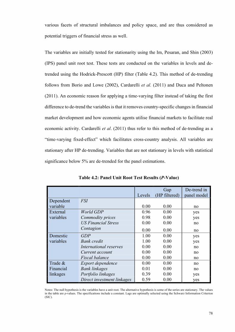
literature. The initial analysis addresses a knowledge gap in the measurement of financial
stability. Existing measures of financial stability could not simultaneously: (1) reflect
stability at a systemic scale; (2) reflect stability with little lag, and (3) incorporate
information on the financial structure of the economy. Financial Stress Indices (FSI) are
constructed to address these deficiencies. The FSIs are constructed using indicators of
stress and weighted using the liability side of the financial structure of the sample
economies. The indicators and weights of the FSIs span four major market segments - the
equity market, banking system, domestic bond market and foreign finance market. Using
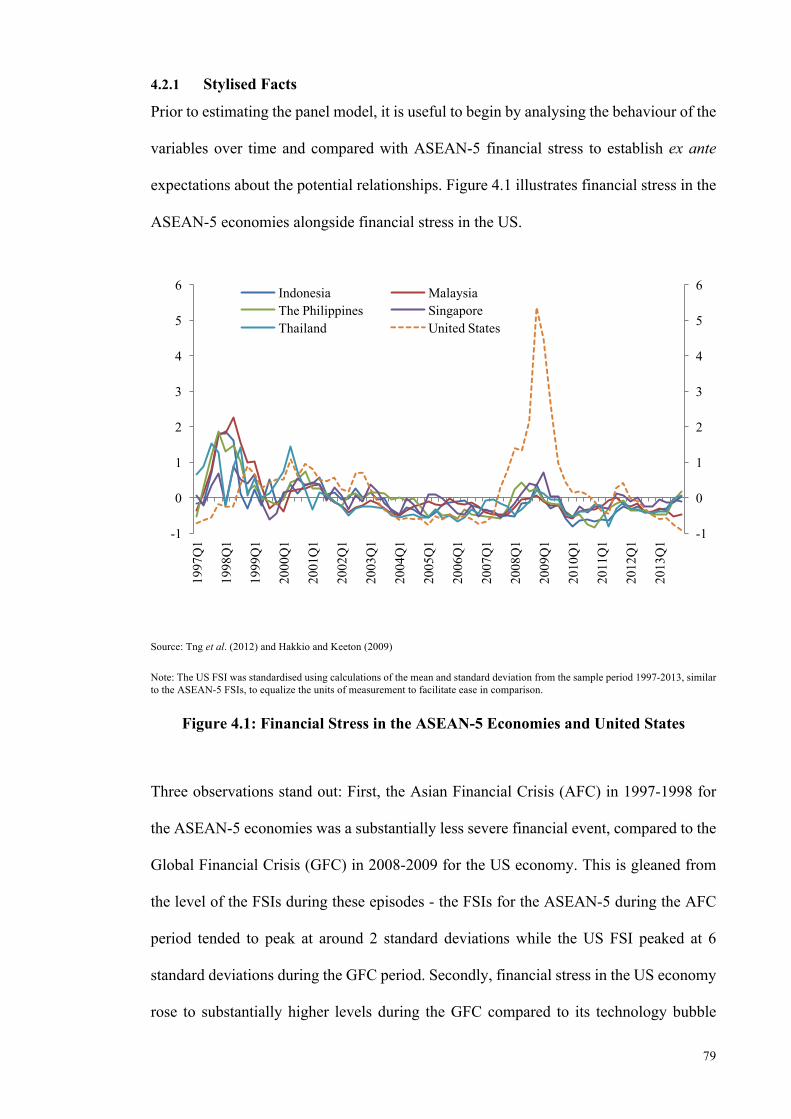
data from 1997-2013, the results reveal three periods of higher financial stress. The most
severe episode in terms of magnitude and duration was the Asian Financial Crisis (1997-
1998). This is followed by the US technology bubble burst (tech bust) (2000-2001) and
the recent Global Financial Crisis (GFC) (2007-2009). Interestingly, higher stress levels
were seen during the tech bust compared to the GFC in all countries, except Singapore.
The FSIs are subsequently modelled as a panel model to investigate the sources of
financial stress in the ASEAN-5 economies. The methodology and model specification
extends from the Early Warning System (EWS) literature by: (1) including more external
variables to better capture the open-economy aspect; (2) including a measure of regional
financial contagion; (3) analysing the entire financial cycle instead of just crisis periods,
and; (4) using an instrumental variable approach to address endogeneity concerns. The
results show that: US financial stress and regional financial contagion are significant
common determinants. For country-specific variables, only bank credit emerged as
consistently significant. A positive bank credit gap portends higher financial stress.
Analysis of the sources of financial stress within individual markets reveals the
iv
importance of the banking system and equity markets for financial stress elsewhere.
Country-specific Structural Vector Autoregression (SVAR) models for each ASEAN-5
economy are then estimated to analyse the impact of financial stress on the economy and
the relationship between monetary policy and financial stress. The SVAR models are
adapted to be suited for small-open economies, by including more external variables and
in the model structure, where the external variables affect the domestic variables, but not
vice versa. The models incorporate FSIs to reflect financial stress in the global
environment and ASEAN-5 economies. The findings show that higher financial stress
leads to tighter domestic credit conditions and lower economic activity in all five
countries. The impact on the real economy displays an initial rapid decline followed by a
gradual dissipation. In Malaysia, the Philippines and Thailand, the central banks reduce
policy interest rates (IRs) when financial stress increases, although there is substantial
cross-country variation in the magnitude and time dynamics. Lower policy IRs are found
to have little significant effects in lowering financial stress, but are still effective in
stimulating economic activity through other channels.
v
ABSTRAK
Berdasarkan data dari Indonesia, Malaysia, the Philippines, Singapore dan Thailand
(ASEAN-5), tesis ini menyumbangkan tiga aspek dari segi analisa empirik yang
ditimbulkan dari Kegawatan Ekonomi Sedunia (GFC) pada tahun 2007-2009. Tesis ini
bertujuan memberi hasil penyelidikan yang baru dari segi kes ekonomi yang kecil,
terutamanya kerana terdapatnya kekurangan tinjauan dalam kajian literatur. Bab 3
memberi tinjauan dari segi ukuran metrik kepada stabiliti kewangan. Indek Financial
Stress dibina (FSI) berdasarkan penunjuk tegangan yang diperolehi dari pemberat dari
empat pasaran, iaitu pasaran ekuti, sistem perbankan, pasaran bon domestik dan pasaran
kewangan asing. Bab 4 menganggarkan satu model panel berdasarkan FSI untuk
mengkaji punca tegangan kewangan dalam ekonomi ASEAN-5 ini. Panel yang
ditubuhkan merangkumi kajian sistem ‘Early Warning’ (EWS) yang dapat memerangkapi
sifat empirik yang umum. Keputusan empirik yang umum ini menunjukkan bahawa
kedua-dua variabel luaran (KDNK dunia yang lebih tinggi, tegangan kewangan di US,
dan penularan kewangan di serantau) serta variabel dalaman (keadaan kredit yang
semakin longgar dan aktiviti ekonomi yang bertambah perlahan) menyumbangkan
tegangan pasaran kewangan yang lebih tinggi di ekonomi ASEAN-5. Bab 5
menggunakan pendekatan ‘structural vector autoregression’ (SVAR) untuk menganalisa
impak tegangan kewangan dalam ekonomi, serta hubungan di antara tegangan ekonomi
dan polisi monetari dalam ekonomi ASEAN-5. Keputusan empirik yang diperolehi
mencadangkan bahawa pertambahan dalam tegangan kewangan akan menyebabkan
keadaan kredit yang bertambah tegang serta aktiviti ekonomi yang semakin lembab di
kelima-lima ekonomi serantau ASEAN. Didapati juga bank pusat dari tiga buah negara
utama ini, iaitu Malaysia, the Philippines and Thailand, mempunyai tendensi polisi untuk
mengurangkan kadar bunga apabila tegangan kewangan bertambah (walaupun wujudnya
perbezaan variasi bersilang dari segi magnitud dan dinamik masa). Polisi kadar bunga
vi
yang lebih rendah didapati tidak memberi sebarang kesan yang signifikan terhadap
pengurangan tegangan kewangan. Walau bagaimanapun, polisi bunga a-la rendah ini
adalah efektif dalam merangsangkan aktiviti ekonomi dari resesi melalui saluran
transmisi yang lain.
vii
ACKNOWLEDGEMENTS
This thesis would not have been possible without the pivotal roles played by many people.
First, I thank my supervisor, Dr. Kwek Kian Teng, for her continuous support and believe
in me throughout the years. Her words always motivated me to persevere when most
needed and her advice always guided me in the correct direction.
My ex-boss at RAM Holdings, Dr. Yeah Kim Leng, deserves special mention for giving
me the initial push to pursue this degree and indulging me in many conversations over
research topics. My current bosses, Fraziali Ismail and Dr. Mohamad Hasni Sha’ari at
Bank Negara Malaysia, were instrumental support pillars. They always supported my
studies, shared their thoughts over my research and created an unbelievably conducive
environment for me to study while pursuing my duties at the central bank. I am also
grateful to my colleagues at Bank Negara Malaysia - Ahmad Othman, Dhruva Murugasu,
Dr. Ahmad Razi and Lim Wei Meen - for participating in discussions, sharing advice and
assistance on specific issues that popped up along the way.
Most importantly, I want to thank my wife, Daisy, for being my guardian angel. This
really would not have been possible without her support. She kept the household in order,
kept me sane through the toughest times, made sure I was always well nourished and
always had encouraging words for me. My two children, Nat and Nate, deserve
honourable mention for always making me smile and distracting me when I needed a
break.
viii
TABLE OF CONTENTS
Abstract ............................................................................................................................ iiiAbstrak .............................................................................................................................. v
Acknowledgements ......................................................................................................... viiTable of Contents ........................................................................................................... viii
List of Figures .................................................................................................................. xiList of Tables ................................................................................................................. xiii
list of Abbreviations ....................................................................................................... xivList of Appendices ......................................................................................................... xvi
1.2 Research Problem .................................................................................................... 41.3 Research Objectives ................................................................................................ 5
1.4 Outline of the Thesis ............................................................................................... 7
: LITERATURE REVIEW .................................................................. 10
2.1 Introduction ........................................................................................................... 102.2 A Historical Context of how Financial Factors Feature Models for Monetary Policy
2.2.1 From Large Scale Models to Monetary Rules ......................................... 122.2.2 From Monetary Rules to Interest Rate Rules ........................................... 14
2.3 The Taylor Rule in Macroeconomic Models ......................................................... 152.3.1 New Keynesian Models ........................................................................... 16
2.3.2 Vector Autoregression Models ................................................................ 172.3.3 Incorporating Financial Factors into Models with Taylor Rules ............. 19
2.3.4 Financial Stability and Crises in Macroeconomic Models ....................... 202.4 Measuring Financial Stability: The Financial Stress Index ................................... 22
2.4.1 The Early Warning Indicators of Financial Crisis ................................... 222.4.2 Current Financial Stress Indexes .............................................................. 23
2.4.3 Building on Existing FSIs for ASEAN-5 Economies .............................. 252.5 The Sources of Financial Stress ............................................................................ 27
2.5.1 Early Warning Indicators of Financial Crisis ........................................... 272.5.2 Spillovers from External Financial Episodes ........................................... 28
2.5.4 Recent Investigations of Financial Spillovers using FSIs ........................ 332.6 Financial Stress, Real Economic Activity and Monetary Policy .......................... 36
2.6.1 How Financial Stress Affects Real Economic Activity ........................... 362.6.2 The Role of Monetary Policy and How Monetary Policy Transmission
Changes during Episodes of Financial Instability .................................... 402.6.3 Utilising FSIs to Measure Interactions in the Real Economy, Financial
Instability and Monetary Policy ............................................................... 432.7 Conclusion ............................................................................................................. 45
: THE MEASUREMENT OF FINANCIAL STRESS IN ASEAN-5 ECONOMIES ................................................................................... 46
3.2.1 Data .......................................................................................................... 473.2.2 Constructing the Financial Stress Index ................................................... 48
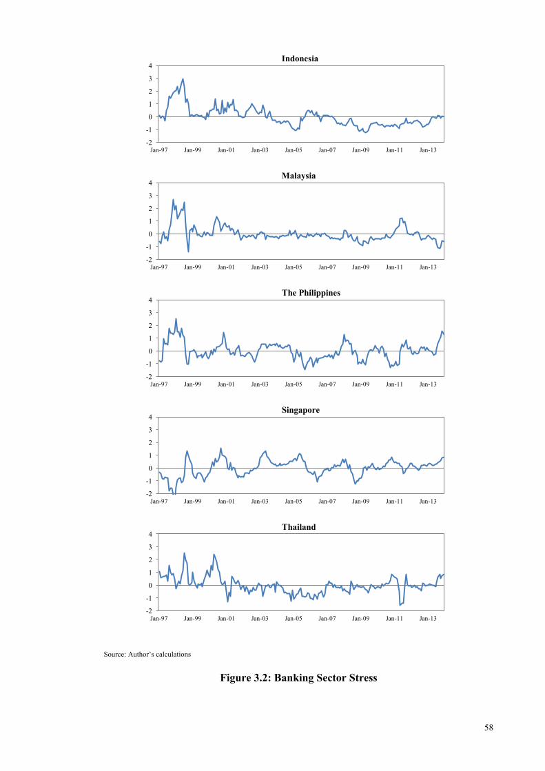
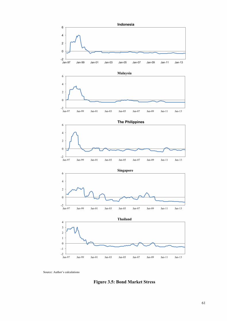
3.3.1 Stylised Characteristics of Financial Stress in the ASEAN-5 .................. 553.3.2 A Historical Perspective of Financial Episodes ....................................... 62
3.4 Robustness of the FSIs to other Weighting Methodologies .................................. 693.5 Conclusion ............................................................................................................. 72
: SOURCES OF MACR-FINANCIAL VULNERABILITIES IN ASEAN-5 ECONOMIES ................................................................. 73
4.1 Introduction ........................................................................................................... 734.2 Data ................................................................................................................... 76
4.2.1 Stylised Facts ........................................................................................... 794.3 The Panel Model .................................................................................................... 87
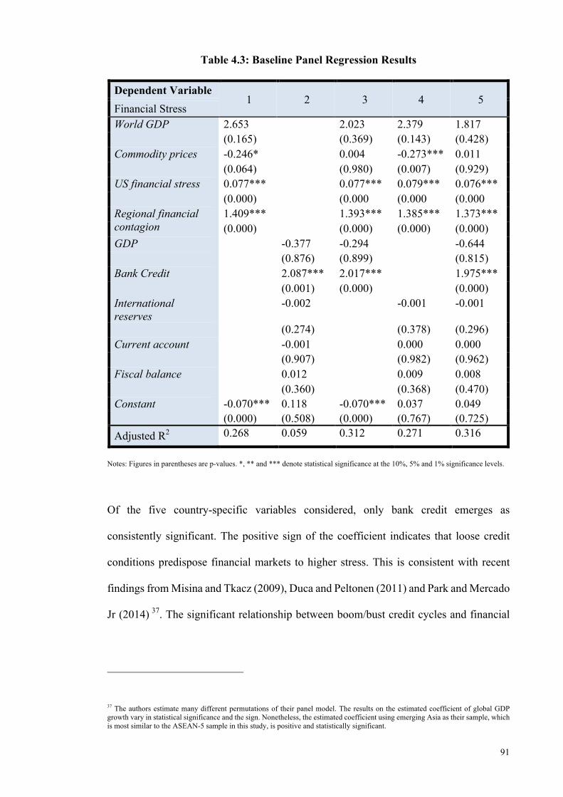
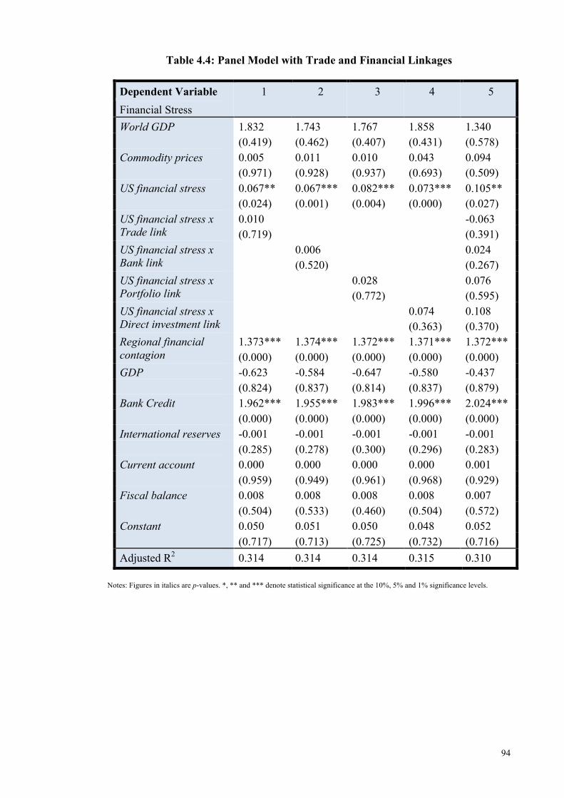
4.4 Baseline Estimation Results .................................................................................. 904.5 Trade and Financial Linkages in the Transmission of External Financial Shocks 92
4.6 Endogeneity and Instrumental Variables Estimation ............................................ 954.6.1 Panel Granger Testing to Investigate the Direction of Causality ............. 95
4.6.2 Addressing Endogeneity with Instrumental Variable Estimation ............ 974.7 The Sources of Financial Stress across Asset Markets ......................................... 99
: THE IMPACT OF FINANCIAL STRESS ON ECONOMIC ACTIVITY AND MONETARY POLICY TRANSMISSION IN ASEAN-5 ECONOMIES ............................................................... 104
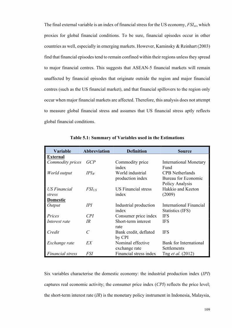
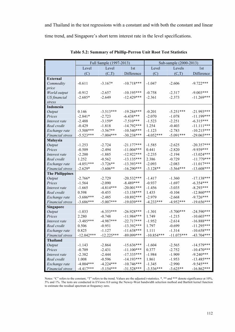
5.2.1 Data ........................................................................................................ 1085.2.2 Unit Root Testing ................................................................................... 110
5.2.3 Specification Issues ................................................................................ 1135.2.4 The Structural Vector Autoregression (SVAR) Model .......................... 114
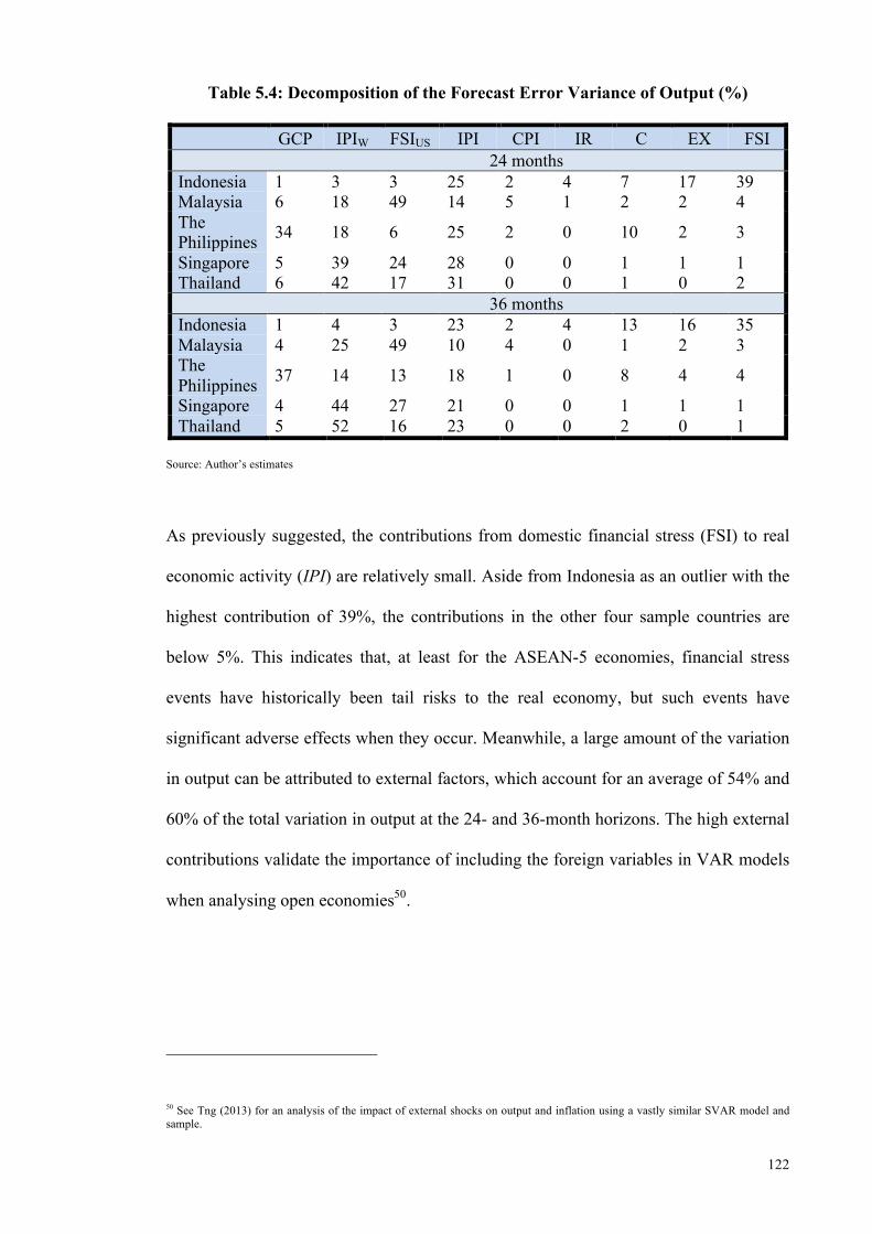
5.3 Results ................................................................................................................. 1185.3.1 The Impact of Financial Stress ............................................................... 118
6.1 Introduction ......................................................................................................... 1306.2 Main Contributions and Findings ........................................................................ 131
6.3 Practical Implications .......................................................................................... 1346.3.1 Improving the Communication of Financial Stress ............................... 134
6.3.2 Reducing Forecast Errors of Economic Activity and Quicker Policy Responses ............................................................................................... 136
6.3.3 Combining Micro-Level Supervision with Macro-Level Surveillance .. 1376.3.4 Need for Increased Corporation among Regional Central Banks and
Supervision Authorities .......................................................................... 1386.4 Further Research Opportunities ........................................................................... 139
Figure 3.5: Bond Market Stress ...................................................................................... 61
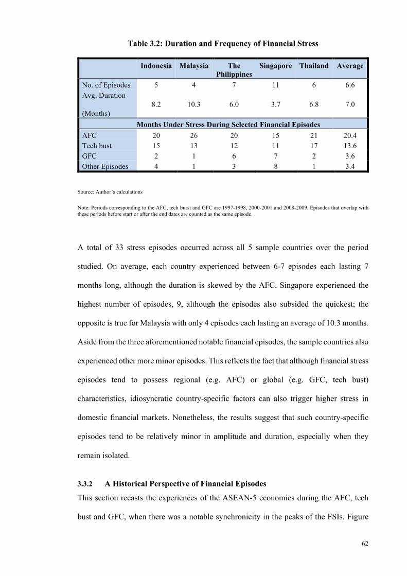
Figure 3.6: Contribution of Market Segments to Overall Financial Stress across Financial Episodes (Share, %) ........................................................................................................ 63
Figure 3.7: Proportion of Countries under Financial Stress ........................................... 66
Figure 3.8: Comparison of FSIs with Alternative Weighting Methodologies ................ 70
Figure 4.1: Financial Stress in the ASEAN-5 Economies and United States ................. 79
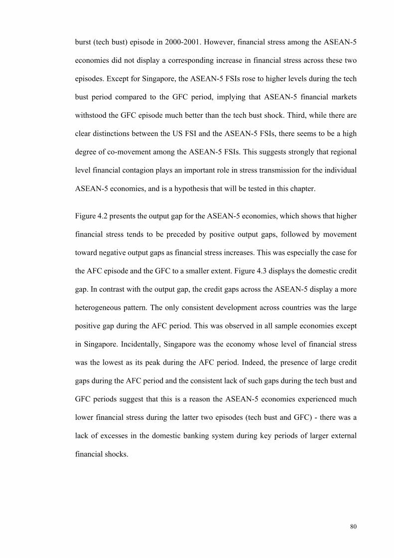
Figure 4.2: Domestic Output Gaps in the ASEAN-5 Economies ................................... 81
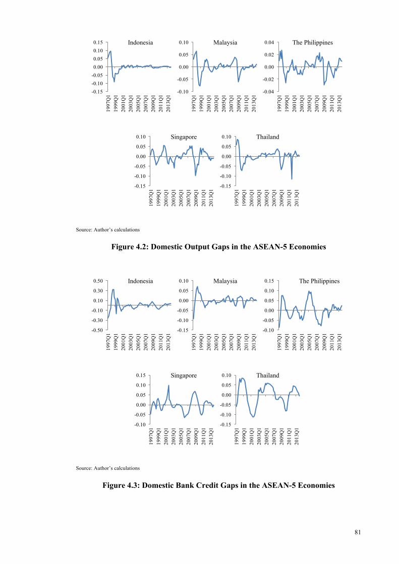
Figure 4.3: Domestic Bank Credit Gaps in the ASEAN-5 Economies ........................... 81
Figure 4.4: Current Account Balance in the ASEAN-5 Economies (% of GDP) ........... 82
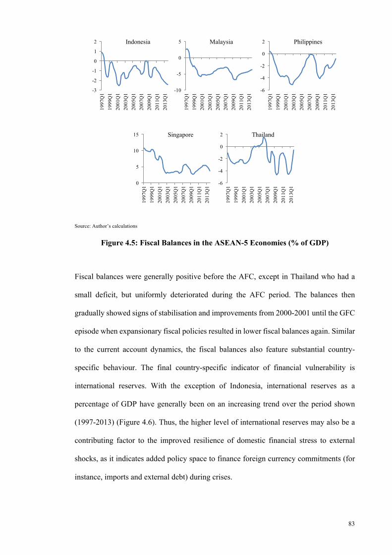
Figure 4.5: Fiscal Balances in the ASEAN-5 Economies (% of GDP) .......................... 83
Figure 4.6: International Reserves (Excluding Gold) in the ASEAN-5 Economies (% of GDP) ............................................................................................................................... 84
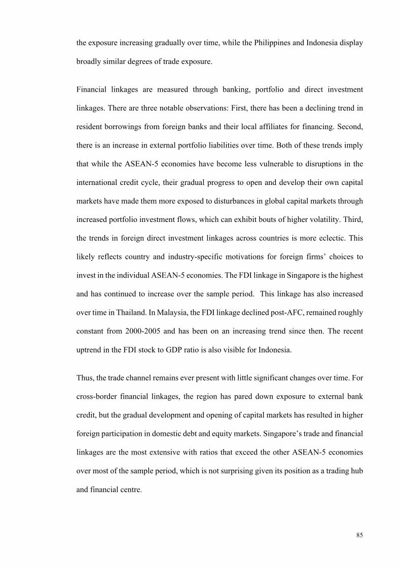
Figure 4.7: Trade and Financial Linkages in the ASEAN-5 Economies ........................ 86
Figure 4.8: Measure of ASEAN-5 Regional Financial Contagion ................................. 89
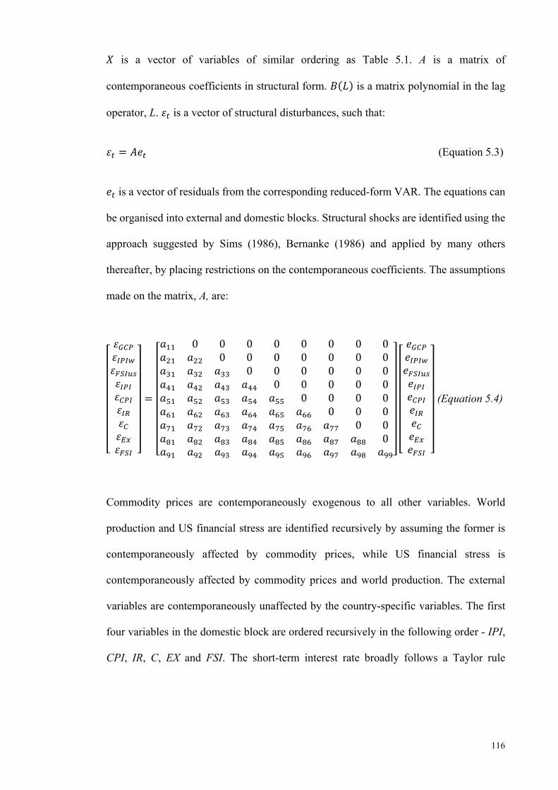
Figure 5.1: Causality Assumptions in the VAR Model ................................................ 115
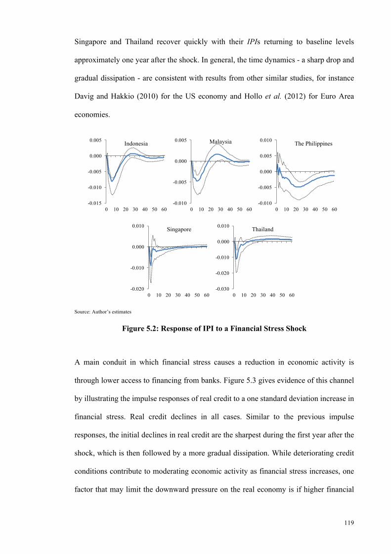
Figure 5.2: Response of IPI to a Financial Stress Shock .............................................. 119
Figure 5.3: Response of Real Credit to a Financial Stress Shock ................................. 120
Figure 5.4: Response of NEER to a Financial Stress Shock ......................................... 121
xii
Figure 5.5: Response of Interest Rate to a Financial Stress Shock .............................. 124
Figure 5.6: Response of Financial Stress to an Interest Rate Shock ............................. 125
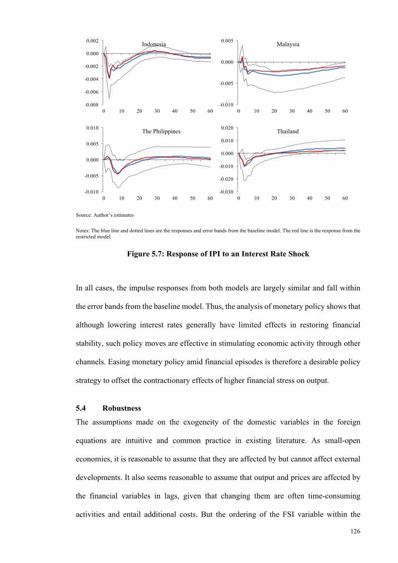
Figure 5.7: Response of IPI to an Interest Rate Shock ................................................. 126
Figure 5.8: Impulse Responses from Alternative Ordering Assumptions .................... 129
Figure 6.1: Sample Heat Map Applied to Asian Economies ........................................ 136
xiii
LIST OF TABLES
Table 2.1: Summary of FSIs from Early Studies ............................................................ 26
Table 3.1: Financial Structure in ASEAN-5 Economies ................................................ 53
Table 3.2: Duration and Frequency of Financial Stress .................................................. 62
Table 3.3: Local and Global Peaks in Financial Stress ................................................... 67
Table 4.1: List of Variables for Panel Estimation ........................................................... 77
Table 4.2: Panel Unit Root Test Results (Ρ-Value) ........................................................ 78
SBI : Sertifikat Bank Indonesia (Bank Indonesia Certificates)
SIC : Schwartz Information Criterion
SVAR : Structural Vector Autoregression
US : United States
UK : United Kingdom
VAR : Vector Autoregression
xvi
LIST OF APPENDICES
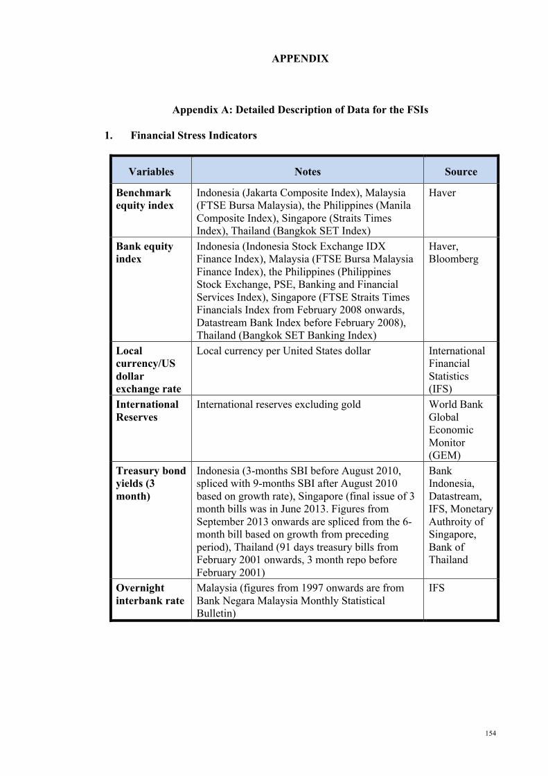
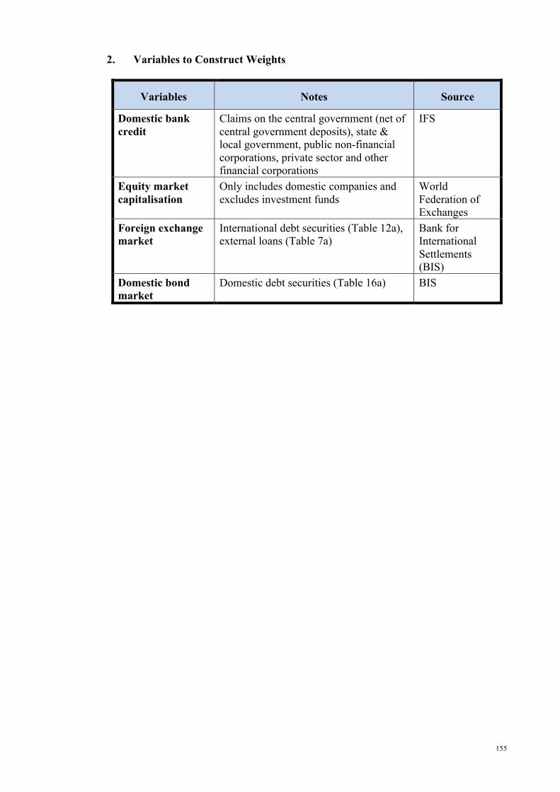
Appendix A: Detailed Description of Data for the FSIs ............................................... 154
Appendix B: Results from Principal Component Analysis to Derive Weights for Measure of Regional Financial Contagion .................................................................................. 156
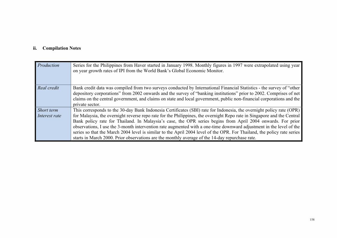
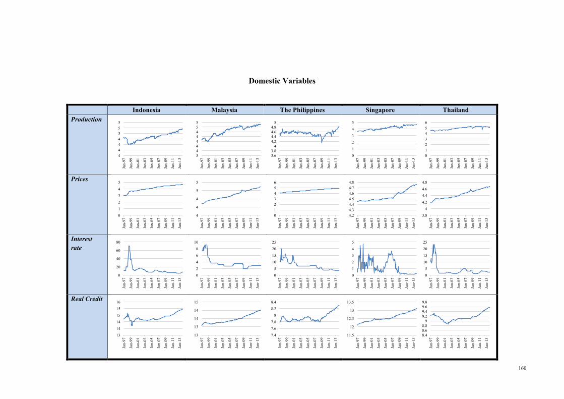
Appendix C: Data Appendix for the SVAR Models .................................................... 157
1
: INTRODUCTION
1.1 Background
Financial crises are events that demonstrate how interlinked financial markets are with
the real economy. Economic contractions are deeper and recoveries take longer during
business cycle downturns that are associated with financial crises (Reinhart & Rogoff,
2009, 2014). It is therefore pertinent to have a robust framework to monitor financial
stability conditions and knowledge of the available policy options to restore growth and
financial stability during crisis periods.
However, financial crisis and financial (in)stability are often seen as binary events in the
financial crisis literature. Specifically, the literature on identifying Early Warning
Indicators (EWIs) of financial crisis is premised first on viewing financial market
conditions as either stable or in crisis, and subsequently identifying the indicators that
foreshadow an impending financial crisis. There is an inherent gap in the measurement
of financial stability conditions between the states of “no crisis” and “crisis”. It is hence
difficult to fully grasp the severity of an impending financial crisis as it starts as an
isolated event within a specific asset market to when it becomes a systemic crisis event.
Consequently, it is also difficult to comprehend the eventual effects of the crisis on the
real economy and, hence, the necessary policy actions to restore macroeconomic stability.
This limitation was highlighted during the Global Financial Crisis (GFC) of 2007-2009.
Take for example, the International Monetary Fund’s (IMF’s) outlook for the global
economy during this period. Figure 1.1 illustrates that the IMF’s forecast of global growth
for 2009 in 2008 was only for a moderate slowdown, but still positive. This was even
after Lehmann Brothers investment bank failed in September 2008, which sent the crisis
into a substantially more intense phase. When the IMF released their global forecasts the
2
following month, in October 2008, the scale of the crisis’ impact on the real economy
was still not yet appreciated. This is seen in the large errors in forecasts made in 2008. It
was only in 2009 itself that the agency substantially revised downward growth forecasts
that were close to the actual figures.
Source: International Monetary Fund World Economic Outlook (Various Issues)
Figure 1.1: IMF’s Forecast of 2009 Gross Domestic Product Growth
The main reason for this uncertainty during the GFC and financial crises in general is that
there is a lack of high frequency indicators that reflect the escalation of the crisis from its
nascent stage, when it is still isolated to individual asset markets to when it becomes a
systemic event. This makes it difficult to monitor the progression of the financial crisis
in real time. Among the available indicators are individual asset prices and the aggregate
balance sheets of economic agents. However, asset prices reflect stress only in specific
market segments, while aggregate balance sheet information is often highly lagged since
reporting standards only require collection at pre-specified periods at low frequency (e.g.
usually quarterly or annually).
3.8
1.3
6.6
3.0
0.5
6.1
0.5
-2
3.3
-1.3
-3.8
1.6
-1.1
-3.4
1.7
-0.6
-3.2
2.4
-6
-4
-2
0
2
4
6
8
World Advanced Economies Emerging Economies
YoY, %
Apr-08 Oct-08 Jan-09
Apr-09 Oct-09 Actual
3
In a “crisis” and “no crisis” paradigm, there is a risk that policymakers are jolted into
policy action only after a crisis is triggered. In addition, the uncertainty over financial
stability conditions cascades to uncertainty in growth forecasts and the formulation of
policy responses. This leads to effective policy actions being hampered by a lack of clarity
in terms of: (1) whether a change in policy is warranted given the effects that the financial
crisis is anticipated to have on macroeconomic stability (growth and inflation), and; (2)
uncertainty over the effectiveness of specific policy instruments given the stress in
financial markets.
These aspects of policy uncertainty were openly and explicitly expressed by major central
banks during the GFC period. The first type of uncertainty is echoed in the European
Central Bank’s (ECB) press statement on 2nd October 2008, when they decided to leave
their monetary policy stance unchanged:
“…it needs to be stressed that we face an extraordinarily high degree of
uncertainty, in large part stemming from the recent intensification of the financial
market turmoil. This complicates any assessment of the near to medium-term
economic prospects.” (European Central Bank, 2008)
This judgment reflects the view that as the GFC entered an intense phase (after Lehmann
Brother’s failed on 15th September 2008), the ECB’s monetary policy consideration was
complicated by difficulties in assessing growth prospects due to uncertainties over the
impact of the financial crisis. There was thus an indication of policy paralysis that is
attributable to the uncertainty over economic prospects.
The second aspect of uncertainty was echoed by the United States (US) Federal Reserve
Bank’s Federal Open Market Committee (FOMC) as they deliberated on monetary policy
4
in 2008 amid the crisis. The following is an excerpt taken from the minutes from the
meeting held in October 2008:
“Some members were concerned that the effectiveness of cuts in the target federal
funds rate may have been diminished by the financial dislocations...” (Board of
Governors of the Federal Reserve System, 2008)
Even after the US Federal Reserve Bank began easing monetary policy by this meeting,
there was disagreement among members over the effectiveness of the interest rate
changes on the real economy, primarily because of different beliefs over changes in the
monetary transmission mechanism brought about by the financial crisis.
1.2 Research Problem
As the previous section highlights, there is currently a knowledge gap in the measurement
of financial stability conditions on a continuous scale. This drawback in turn limits
analyses of other issues that are pertinent for the assessment of macro-financial
vulnerabilities and the appropriate monetary policy responses during crisis periods.
Specifically, this thesis attempts to address the following three drawbacks in existing
literature:
I. The measurement of financial crises in existing financial crisis studies take on a
binary nature - crisis or no crisis. There are two adverse consequences of this
approach. First, this measurement approach does not allow the monitoring of
financial stability conditions from when stress initially emerges within individual
asset markets, to when it becomes a systemic financial crisis. Second, this
measurement approach results in studies that do not account for periods that are
marked by higher stress in financial markets, but without systemic failures of
financial institutions, currency runs or sovereign debt defaults. While not fitting
the traditional definition of crises, such episodes are nonetheless significant if they
5
had large adverse macroeconomic effects (Borio & Lowe, 2002), and hence
deserve more attention.
II. The established empirical commonalities from EWI studies implicitly assumes
that crisis periods are different from normal periods, while being silent on the
possibility that changes in financial stability conditions may result from large
movements in the explanatory variables. While it is relatively clear what the early
warning indicators of financial crises are, less clear is what drives the remaining
parts of the financial cycle.
III. The lack of a continuous measure of financial stability has largely constrained
time series analysis of the impact of adverse financial shocks on: 1. Economic
activity and its transmission mechanism, and: 2. how monetary policy
transmission is affected by episodes of financial instability. This is especially true
for economies with a low frequency of historical incidences of financial crises.
1.3 Research Objectives
Accordingly, the main objectives of this study are to:
I. Measure financial stability conditions on a continuous scale. This is achieved by
constructing an index called the Financial Stress Index (FSI) that is capable of
reflecting financial stress as it emerges from low levels within individual asset
markets, to high levels as financial stress spreads across asset markets and become
systemic events. This later stage is what current literature often recognises as a
financial crisis.
II. Identify the sources of financial stress throughout the entire financial cycle. This
helps to shed light on the factors that determine financial stress beyond just
financial crisis periods.
6
III. Estimate the dynamic impact of financial stress on the real economy, the
transmission channels and how monetary policy effectiveness changes relative to
financial stability conditions.
To the extent that there has been a resurgence of interest in these issues especially since
the GFC episode, studies that attempt to address them have focused largely on developed
economies, where the GFC played centre stage and have eschewed emerging and small-
open economies. Undoubtedly, the findings from studies of large developed economies
do not automatically apply to emerging and small-open economies. This is because the
latter economies tend to have less developed financial markets and different institutions
as well as regulatory structures. They also tend to be more vulnerable to sudden reversals
in capital flows and external developments. For emerging and small-open economies, a
modelling strategy that is distinct from the approach applied on developed economies is
hence needed to address the aforementioned issues.
This thesis uses 5 small-open economies from Asia for the empirical analysis - Indonesia,
Malaysia, the Philippines, Singapore and Thailand (ASEAN-5). This sample is chosen
among the other small-open economies primarily for three reasons. Firstly, the ASEAN-
5 economies experienced their own financial crisis over a decade earlier in 1997 and
underwent significant structural reforms thereafter in efforts to improve the resilience of
its financial markets and economies. When comparing systemic financial stability
conditions across time and countries, this event provides a useful benchmark of relative
severity and changes in resilience during subsequent financial episodes such as the
technology bubble burst in the United States in 2000-2001 and the GFC in 2007-2009.
Secondly, these 5 economies possess diverse economic structures. For instance,
Singapore is a newly industrialised country with developed and open financial markets,
while Malaysia and Indonesia are commodity rich economies who export both food and
7
fuel. This diversity can help pin down whether the derived empirical findings to the
questions posed are country-specific or robust to differences in economic and financial
market structures. Finally, as will be shown in subsequent chapters, for the questions
posed in this thesis, there is relatively less literature for the selected sample. This is
attributable in part to limitations in data availability. There is, in general, less publically
available data for emerging economies that span a sufficiently long time period that
contains a rich enough set of events to analyse these issues. With the AFC, the technology
bubble burst, the recent GFC and subsequent euro debt crisis, the ASEAN-5 economies
have recently experienced a sufficiently rich variety of domestic and external financial
shocks over the last two decades to facilitate a meaningful analysis of the various facets
of financial stability, macro-financial vulnerabilities and how financial stability
conditions affect monetary policy transmission.
1.4 Outline of the Thesis
The remaining chapters are organised as follows:
Chapter 2 conducts a review of the existing literature. This review sets a historical
context of the current state of literature and then traces the evolution of relevant sub-fields
to their current stage of development. Finally, the research problems that this thesis
attempts to address are highlighted.
In Chapter 3, a methodology is developed to measure financial stress on a continuous
scale. These measures are presented as indices called, Financial Stress Indices (FSIs), and
reflect stress in specific asset markets and at the overall systemic level. Low and high
values reflect, respectively, buoyancy and distress in financial markets. The overall FSI
for each country is a weighted-average of its market-specific FSIs, with weights that
reflect the relative share of financing sourced from the individual market segments.
Specifically, the shares reflect the significance of each represented market segment in
8
providing financing to economic agents. This is done to tailor the FSIs to the differing
financial structures across the sample countries and their evolution over time. The FSIs
are then used to analyse facets of financial episodes in the region from 1997-2013. This
includes the frequency, duration and magnitude of higher stress episodes, and the
contribution of stress from individual asset markets to overall financial stress during such
episodes. The FSIs provide the basis and starting point for the analyses conducted in
chapters 4 and 5.
Chapter 4 determines the sources of financial stress in the ASEAN-5 economies using a
panel data methodology. The panel model is constructed with the FSIs modelled as a
function of common global and regional variables, and a set of county-specific
vulnerability indicators that EWI studies have traditionally focused on. Two notable
contributions are made in this chapter: First, the analysis uses an instrumental variable
approach to control for endogeneity arising from two-way causality between financial
stress and the domestic variables (e.g. GDP, current account balances, fiscal balances and
international reserves). Second, the panel analysis is subsequently conducted on the
market-specific FSIs (representing stress in the banking system, equities, foreign
exchange and bond market), to investigate if the sources of financial stress are similar
across asset markets and to give insight to how financial stress spreads across asset
markets.
In Chapter 5, the FSIs are embedded in an open-economy Structural Vector
Autoregression (SVAR) model for each ASEAN-5 economy to analyse the transmission
of financial stress to the real economy and how financial stress affects the transmission
of monetary policy. The model structure explicitly incorporates a small-open economy
assumption, in which global variables affect the country-specific variables, but not vice
versa. Impulse response functions from the estimated SVAR models are used to
9
characterise the speed and depth of the economic downturn in response to adverse
financial shocks. This methodology is also utilised to give insight to the roles of credit
and the exchange rate in the transmission of financial stress. Finally, impulse response
analysis is used to quantify the role of financial stress in altering the transmission of
monetary policy to the real economy.
The final chapter, Chapter 6, concludes with a summary of the main findings of this
thesis. The policy implications are then drawn from the findings especially when viewed
from a broader context. This includes areas of policy-oriented surveillance, regional
cooperation and the conduct of monetary policy. Finally, the chapter discusses some
potentially fruitful avenues for further research going forward.
10
: LITERATURE REVIEW
2.1 Introduction
The Global Financial Crisis (GFC) of 2007-2009 was, in some aspects, a teachable
moment to the limitations of existing macroeconomic models’ usefulness for macro-
financial surveillance and policy guidance. For central banks, in the two decades or so
prior to the GFC, the conduct of monetary policy was guided predominantly through the
lens of a “Taylor Rule”, in which the policy instrument, usually a short-term interest rate,
is modelled as a function of inflation and output. This simplistic paradigm became widely
accepted since being introduced because using it for policy guidance seemed to yield
successful results as business cycle fluctuations and inflation moderated during the 1980s
till the early 2000s. Indeed, many attributed the improved macroeconomic stability to the
better management of monetary policies.
Since the GFC, these views have been largely reversed by policymakers and academics
alike, and have been articulated particularly forcefully in Blanchflower (2009), Bean,
Paustian, Penalver, and Taylor (2010) and Solow (2008). To illustrate, Blanchflower
(2009) lamented the following in March 2009 in the midst of the GFC:
“As a monetary policy maker I have found the ‘cutting edge’ of current
macroeconomic research totally inadequate in helping to resolve the problems
we currently face.”
This chapter starts by reviewing the pre-GFC ideology and the limitations to this approach
that were highlighted by the GFC episode. The review begins with a brief historical
narrative of how macroeconomic models evolved to the state just prior to the GFC
episode. The main narrative put forth is that before the GFC, financial markets and
financial factors were largely ignored or featured with limited scope in models that were
11
used for policy analysis. Post-GFC, the debate shifted focus to how to measure these
financial factors and how to incorporate them into standard macroeconomic models, so
that they can be more useful for surveillance and policy analysis. A sound understanding
of the evolution of macroeconomic models from a historical perspective is necessary, as
it indicates the directions that were taken in the past that were not fruitful and thus should
be avoided going forward.
This literature review then notes the absence of measures of financial instability in
mainstream models. It is plausible that its absence may be attributable to the observation
that episodes of elevated financial stress are relatively infrequent and hence it was okay
to exclude it from the models. However, this perception has largely changed post-GFC.
From an analytical perspective, a major hurdle for its exclusion is due to the lack of
explicit measures of financial instability. Subsequently, the review traces the progression
of three lines of literatures up to their current stage of development. These literatures
pertain to: 1. The measurement of financial stability conditions; 2. An explanation of the
determinants of financial stability throughout the financial cycle, and; 3. The real
economic effects of adverse financial shocks and how monetary policy transmission is
affected by financial (in)stability. The limitations in current knowledge are established
and are the bases for the analyses in the remainder of this thesis.
The remaining sections proceed as follows: Section 2.2 provides a historical context of
how financial factors featured in past macroeconomic models. Section 2.3 discusses the
advent of Taylor Rules, its incorporation into models for policy analyses, how it was
expanded over time and notes that measures of financial stability were missing from such
models. Section 2.4 details the current knowledge on measuring financial stability.
Section 2.5 presents the literature that give insight to the sources of financial stability.
12
Section 2.6 then details the interactions among financial stability, real economic activity
and monetary policy. The last section concludes.
2.2 A Historical Context of how Financial Factors Feature Models for Monetary
Policy Analysis
2.2.1 From Large Scale Models to Monetary Rules
Before looking at how models should progress in the post-GFC era, it is instructive to
first look back at modelling efforts of how financial factors featured in models for
monetary policy analysis from a historical context. This is to gain an understanding of
what the previous efforts were, how successful they were during that era and why they
became outdated.
Among the first frameworks that were developed and used by major central banks for
monetary policy analysis were large-scale econometric models such as the MIT-FRB and
Brookings models, which were used during the 1960s and 1970s (Brayton, Levin, Lyon,
& Williams, 1997). These models consisted of many equations that attempted to account
for the various channels through which policy shifts would affect the real economy. For
instance, over 60 equations in the MTT-FRB model were constructed and estimated to
capture intricate features of the US economy, including the behaviour of the central bank,
state and local governments, commercial banks, the household and business sectors and
“a detailed treatment of the financial sector” (Rasche & Shapiro, 1968). The main goal
was to have a detailed analytical framework that was not only capable of quantifying the
impact of policy shifts on the real economy, but also how they were transmitted.
These frameworks started to fall out of favour in the mid-1970s for two reasons: Firstly,
the simulation results were unstable and forecasts were unrealistic (Gramlich, 2004).
Secondly, Lucas (1976) argued that the estimated parameters were not suitable for policy
inference. A crucial assumption in these models was that the estimated parameters were
invariant to policy changes, for it enabled the conduct of counterfactual simulations to
13
estimate the impact of hypothetical policy shifts. However, Lucas (1976) pointed out that
because firms and consumers were forward looking, their responses would vary
systematically with policy shifts. This implied that the estimated fixed coefficients were
in fact not fixed, and were thus not valid for policy inference. This line of reasoning is
now known as the “Lucas Critique”.
Following the failure of large-scale econometric models in the 1970s, attention then
turned to frameworks that advocated a targeted rule-based approach to conduct monetary
policy. Though this school of thought, known as monetarism, gained prominence in the
1970s, studies done in the previous two decades provided much of the underlying
foundations.
To begin, empirical findings diminished previously held views over the potency of
monetary policy, from a multiplier of between four and five to about one (De Long, 2000).
Although there was evidence of the short-run non-neutrality of money, it was pointed out
that using monetary policy as a stabilisation tool would likely exacerbate instead of
smooth economic fluctuations because of the uncertain multiplier and lag effects
(Friedman & Shwartz, 1963). These findings supported a rule as opposed to discretion
approach to conducting monetary policy.
The monetarist framework gained widespread credibility when the associated researchers
correctly predicted that the Phillips curve relationship, a downward sloping curve that
characterised a negative correlation between inflation and unemployment, would not hold
over the long-run. It was previously thought that a central bank’s decision simply
involved conducting monetary policy by deciding among pairs of unemployment and
inflation (i.e. a desire to lower the unemployment rate would come at the cost of higher
inflation) (Samuelson & Solow, 1960). This was disputed by Phelps (1967) and Friedman
(1968), who postulated that the trade-off would only hold in the short-run and that the
14
long-run Phillips curve was in fact vertical. Their hypothesis implied that repeated
attempts to stimulate aggregate demand through expansionary monetary policy would
only lead to higher inflation with no decrease in unemployment. This proved correct when
the oil price shocks in the 1970s led to both high unemployment and inflation. This event
marked a turning point for institutional acceptance of the monetarist framework, as the
Federal Reserve and Bank of England adopted fixed targets of the money stock as a policy
rule during the mid-late 1970s (De Long, 2000).
2.2.2 From Monetary Rules to Interest Rate Rules
However, inflation and unemployment continued to increase in response to the oil price
shocks under this new framework of fixed targeting of the money stock. In addition, this
policy led to volatile interest rates, which was regarded as detrimental to economic
activity and hence unemployment. These events eventually led Paul Volker, then
Chairman of the Federal Reserve Bank, to unofficially abandon the monetarist regime in
favour of a discretionary approach in 1979 by using the Federal Funds rate (short-term
interest rate) as the policy variable. Inflation eventually subsided after the Federal Funds
rate was kept high for a sustained period.
Following the failure of the monetarist framework, attention turned to formulating other
simple and robust interest rate rules. A key result of this effort was the following
expression:
! = !∗ + &'(∗ +&)*
∗ (Equation 2.1)
i and i* are the nominal and natural (equilibrium) interest rate. π* is the inflation gap
(inflation - targeted inflation), and y* is the output gap (output - potential output). This
rule relates changes in the nominal short-term interest rate to changes in inflation and
output. For instance, a nominal interest rate increase is expected to lead to lower inflation
and output. Although initially introduced and discussed by (Bryant, Hooper, & Mann,
15
1993), the formula’s applicability for policy was demonstrated clearly by Taylor (1993),
when he proposed the following equation using historical data from the United States as
a guide:
! = 2 + 0.5(∗ + 0.5*∗ (Equation 2.2)
This rule came to be known as the “Taylor rule”. The Taylor rule’s simplicity in intuition,
ease in application and ability to closely fit the historical movements among the Federal
Funds Rate, output and inflation in the United States, has since provided a foundation in
thinking about the practice of monetary policy globally. Nonetheless, Taylor rules were
only single equations which described the output-inflation tradeoff, and were not cohesive
macroeconomic frameworks for application by central banks for policy inference. They
were also often fitted retrospectively using statistical models and still could not account
for structural changes in the economy, thus also making them vulnerable to the Lucas
Critique. Since the monetarist regime was abandoned and due to the lack of a better
alternative, major central banks such as the Federal Reserve Bank continued using their
large-scale macro-econometric models (later ones incorporated versions of the Taylor
rule) to forecast and conduct policy simulations. However, they were used as guides
without full confidence (Gali & Gertler, 2007).
2.3 The Taylor Rule in Macroeconomic Models
The widespread acceptance of Taylor rules led to renewed efforts to embed it into more
complete models that were more useful compared to existing large-scale macro-
econometric models for policy analysis. These efforts can be categorised as falling
broadly into two main groups, whose progression occurred in parallel with each other:
New Keynesian models (NKMs) and Vector Autoregression (VAR) based models.
16
2.3.1 New Keynesian Models
NKMs are Dynamic Stochastic General Equilibrium (DSGE) models and were initially
developed in Goodfriend and King (1997) and Clarida, Gali, and Gertler (1999). The core
of this framework is its general equilibrium structure similar to that of a Real Business
Cycle1 (RBC) model, thus making it immune to the Lucas Critique. A key point of
departure from RBC models is that the introduction of an explicit price setting mechanism
and nominal rigidities meant that monetary policy was non-neutral in the short-run and
could thus influence aggregate output and prices.
The following key equations emerge from the benchmark model (Clarida et al., 1999):
The residuals εy t, επ t and εi t follow a particular process (often AR(1)) and are interpretable
as shocks. E is expectations, y* is the output gap, π is inflation, i is the nominal interest
rate and !∗ is the natural interest rate. Equation 2.3 is interpretable as a dynamic I-S
equation. Equation 2.4 is an aggregate supply equation known as the New Keynesian
Philips Curve, which differs from its traditional counterpart because inflation here is
forward looking and the trade-off is between output and inflation, as opposed to
employment as previously formulated. Equation 2.5 is an interest rate rule similar to the
Taylor rule. ρ is a smoothing parameter that ranges from 0 to 1 and reflects the lag effect
1 RBC models are DSGE models that attempt to explain business cycle fluctuations. These models posit that business cycles are efficient and generated by technology shocks as opposed to monetary factors, and are equilibrium models in the sense that prices adjust instantly in response to the shocks. This feature of RBC models, that markets always clear, meant there is no role for monetary policy in this framework.
17
of past interest rate changes. A key feature of NKMs is that the key equilibrium
relationships result from dynamic optimisation problems by representative economic
agents. The model is then calibrated to the data for policy inference.
The reference model characterised by equations (2.3)-(2.5) has since been extended.
Perhaps the most natural extension was to develop an open-economy equivalent (De
Paoli, 2009; Galí & Monacelli, 2005), in which the exchange rate, trade, the terms of trade
and international financial markets are incorporated. Another extension is to add a
backward looking variable for inflation (Gali & Gertler, 1999). This feature incorporates
the intuition that economic agents set prices by observing past values. Other features have
been added to the reference framework, although the two previously mentioned is the
most widely accepted and validated.
2.3.2 Vector Autoregression Models
NKMs are fully specified models based on constructions of utility maximising behaviour
of economic agents, which are then calibrated for policy analysis. Vector Autoregression
(VAR) models reflect a different approach. Instead of starting with a theoretical model,
VAR models start with data and seek to impose as few assumptions as needed to
econometrically estimate the macroeconomic relationships.
The main econometric issue in monetary policy analysis is how to account for the
endogenous relationships between the policy instrument and inflation and output.
Movements in the policy instrument are likely largely influenced by inflation and output,
which themselves are also influenced by changes in monetary policy. Hence, simple
correlations or reduced form regressions are almost certainly mis-specified and not
suitable for statistical inference. Instead, it is necessary to identify “autonomous”
monetary policy shocks and estimate how the variables of interest, usually inflation or
18
output, respond to these shocks. This led to the development of the Vector Autogression
(VAR) methodology.
Pioneered by Sims (1980), the underlying motivation was to reduce the number of
restrictions that were necessary to structurally identify the parameters in large-scale
macro-econometric models that were prevalent among central banks, such as the
previously mentioned MIT-FRB model. His main contention was that a large number of
the “a priori” restrictions were not sufficiently guided by theory. The following assertion
was made in his seminal paper:
“Many, perhaps most, of the exogenous variables in the FRB-MIT model…are
treated as exogenous by default rather than as a result of there being good reason
to believe them strictly exogenous. Some are treated as exogenous only because
seriously explaining them would require an extensive modelling effort in areas
away from the main interests of the model builders.” (Sims, 1980)
In essence, VARs are multivariate counterparts to AR models. The latter is a single
variable model in which it is a function of its lagged values. In comparison, VAR models
are multivariate models where each variable is a function of its own lags and those of the
other variables in the system. To derive the desired “shocks” that can be used to analyse
the effects of policy, it is necessary to place assumptions, most commonly, on the
contemporaneous relationships as suggested by Sims (1986), Bernanke (1986) and
Blanchard and Watson (1984), or on assumptions of whether the shocks have long- or
short-run effects (Blanchard & Quah, 1989). By placing these restrictions to identify the
corresponding underlying structural models from the reduced-form VAR models, the
resulting models have come to be known as Structural VARs (SVAR).
19
Many variants of VAR and SVAR models have since been developed. Similar to the
progression of NKMs, a line of literature has pursued the development of VAR and SVAR
models that are specifically structured for open-economies. These variants have
necessitated the inclusion of additional variables that are of high relevance to open-
economies, such as the exchange rate, foreign interest rates, the global price level and
external demand (in addition to the domestic ones). Selected references of more recent
open economy VAR-based models include Cushman and Zha (1997), Kim and Roubini
(2000), Genberg (2005) and Maćkowiak (2007).
2.3.3 Incorporating Financial Factors into Models with Taylor Rules
Over time, studies of monetary policy, in particular those that aim to analyse the role of
financial markets in the transmission of monetary policy, have gradually incorporated
other financial factors into the aforementioned macroeconomic models.
Bernanke and Gertler (1989) and Bernanke, Gertler, and Gilchrist (1999) extend the
benchmark New Keynesian Model (NKM) to introduce a feature where the net worth of
borrowers and imperfections in credit markets are central in determining output
fluctuations and, hence, the behaviour of monetary policy. Within the NKM paradigm,
Bernanke and Gertler (1999;2001) and Cecchetti, Genberg, Lipsky and Wadhwani (2000)
(CGLW) analyse the potential welfare gains from central bank responses to equity prices.
More recently, Christiano, Ilut, Motto & Rostagno (2010) calibrate a NKM and find that
there are welfare benefits from expanding the standard Taylor rule to include credit.
Cúrdia and Woodford (2010) analyse the welfare benefits of adding credit and credit
spreads to the Taylor rule. Simulations from their calibrated NKM indicate that there are
welfare benefits from augmenting the Taylor rule to include credit spreads and, to a
smaller extent, credit as well. More recent NKM-based studies, especially those after the
GFC, also assess the role of housing market interactions on the business cycle and related
The development of VAR-based models in incorporating additional features of financial
markets has also progressed in similar vein. While the majority of earlier studies on
monetary policy analysis were premised on identification schemes around the simplified
Taylor rule, it became common for studies to feature a richer presentation of financial
markets through the inclusion of money, credit and asset prices (equity and property) in
the model. This is reflected in the more recent VAR based studies, for instance, by
Morsink and Bayoumi (2001), Bloom (2009), Bean et al. (2010) and Raghavan,
Athanasopoulos, and Silvapulle (2009), to name a select few.
2.3.4 Financial Stability and Crises in Macroeconomic Models
Despite these advances in theory and empirical methodologies, one aspect of NKMs,
VAR-based models and other macro models that has received insufficient attention is
how financial stability conditions and financial crises are measured and integrated into
the macro models.
A reflection of the significant consequence of this shortcoming is that the forecasts
generated by standard macro models during major financial episodes, such as the GFC,
suffer from high forecast errors. This is highlighted in admissions of the inadequacy of
existing forecasting methodologies by large institutions such as the OECD (2014), the
Federal Reserve Bank and the European Central Bank (Alessi, Ghysels, Onorante, Peach,
& Potter, 2014) and the Bank of England (Stockton, 2012) during the GFC episode. In
these “post-mortem” studies, the two key attributable factors cited were the failure of
macro models to appropriately account for financial market conditions and the size of the
feedback loops between financial conditions and the real economy (Alessi et al., 2014).
Another reflection of inadequate incorporation of financial stability conditions in macro
models was the lack of guidance on how monetary policy effectiveness was affected by
the financial crisis. This led to both sides of the policy divide being taken with a lack of
21
convincing empirical evidence. For example, Mishkin (2009) argues that monetary policy
was effective, indeed more so during crisis periods, because it lowers the chances of
adverse feedback loops between deteriorating financial market conditions and real
economic activity. In contrast, Bouis, Rawdanowicz, Renne, Watanabe, and Christensen
(2013) postulate that monetary stimulus did not provide noticeable improvements to GDP
growth because of a breakdown in the credit channel and the decline in the natural interest
rate. The lower nominal interest rates from monetary policy easing thus did not translate
to higher growth. Bech, Gambacorta, and Kharroubi (2014) also claim that lowering key
policy interest rates during financial crises does not lead to higher growth, mainly because
of a breakdown in the monetary transmission mechanism. These conclusions are arrived
at largely through qualitative argument, reduced-form Taylor rule estimations with
constant and time-varying natural interest rates, or pairwise correlations during crises and
normal periods.
Thus, before the GFC, there was a relative dearth of efforts to measure financial stability
conditions explicitly, analyse how they influence aggregate growth dynamics and,
importantly, how higher instability in financial markets affect monetary policy
transmission and effectiveness. At best, financial crisis periods, which are special cases
of financial stability conditions as it reflects unusually high levels of financial instability,
are included as dummy variables. These shortcomings in current knowledge serve as the
main motivation for this thesis.
The remainder of this chapter explores three strands of literature to their current stages of
development and highlights research opportunities that this thesis attempts to contribute
to. A key underlying motivation of this research is to provide insight and tools that policy
institutions such as central banks can use for policy guidance and macro-financial
surveillance. The first literature explored pertains to how financial stability can be
22
measured in relatively high frequency (monthly or higher), so that such as indicators can
be used to monitor financial stability conditions continuously as crises progress in
severity, and from when they initially emerge in individual asset markets to when they
become systemic. The second literature explored pertains to current knowledge of what
drives financial stability cycles and the identification of early warning signals of
impending financial crises. This knowledge informs as to what developments in the real
sector and financial markets to monitor closely for financial stability surveillance and
crises prevention efforts. The final line of literature that is explored for further
development pertains to the macroeconomic effects of changes in financial stability
conditions and how monetary policy transmission and effectiveness is affected during
periods of financial instability.
2.4 Measuring Financial Stability: The Financial Stress Index
2.4.1 The Early Warning Indicators of Financial Crisis
A precursor to appropriately incorporating financial stability conditions into mainstream
macroeconomic models is the measurement of these conditions. The development of
Financial Stress Indices (FSIs) reflects these efforts. FSIs were only recently developed,
mainly after the GFC, as a complement to the literature on the Early Warning Indicators
(EWIs) of financial crises. Broadly, EWI studies focus on predicting the onset of crises
and discerning their determinants. However, they often treat the crisis variable as binary
events - crisis or no crisis - and were concerned mainly with specific types of crises, such
as balance of payments, sovereign debt or bank crises (Borio & Drehmann, 2009; Illing
& Liu, 2006). This ignored historical evidence that financial crises often involved more
than one market, which Laeven and Valencia (2008) find to be an unreasonable
assumption2. For instance, the authors categorise financial crises as banking, currency or
2 An except is Kaminsky and Reinhart (1999), as they analyse the interactions between balance of payments and banking crises.
23
sovereign debt crisis and find that 42% of banking crises from 1970-2007 involved a
crisis in at least one other category. Thus, though informative, the EWI literature was
unhelpful for gauging the relative intensity of crises in the overall financial system, while
incidents that were isolated to securities markets were often ignored. In addition, “near
miss” episodes, when the degree of financial stress was not severe enough to be classified
as crises, but were nonetheless widely acknowledged to have had macroeconomic
consequences, are often ignored in this line of inquiry (Borio & Lowe, 2002).
2.4.2 Current Financial Stress Indexes
The development of FSIs reflects an attempt to address these limitations, especially after
the GFC period. They are composite indices constructed from asset prices, which provide
a synthetic measure of stress across the entire financial system and within specific asset
markets. FSIs complement the EWI literature in that they can be used to identify
incidences of financial crises, by defining crises as periods when the FSIs exceed pre-
determined thresholds. The markets that are covered in existing FSIs vary across studies,
but often encompass the equity market, bond market, banking sector and foreign
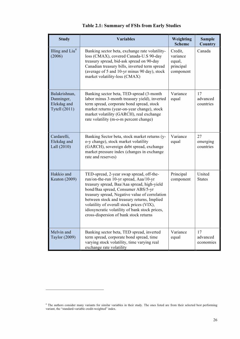
exchange market. Influential studies that construct FSIs are Illing and Liu (2006) for
Canada, Hakkio and Keeton (2009) for the United States, Cardarelli, Elekdag, and Lall
(2011) and Melvin and Taylor (2009) for 17 advanced economies and Balakrishnan,
Danninger, Elekdag, and Tytell (2011) for 26 emerging economies. More have since been
developed in other papers, for instance, by Yiu, Ho, and Jin (2010), Duca and Peltonen
(2011), Tng, Kwek, and Sheng (2012) and Park and Mercado Jr (2014)3.
3 Existing FSI studies have focused primarily on the empirical methodology to construct their respective indices. There is nonetheless an interpretation about the causes and consequences of movements in the FSI that can be drawn from asset pricing and macro-finance theories. The link to asset price theory stems from the fact that FSIs are constructed from asset prices. Conceptually, the price of a financial asset corresponds to the expected discounted payoff that the asset is expected to generate over time. In this formulation of the asset price, the discount factor is dependent on the risk-free rate of return and the risk premium of the asset. Importantly, the risk premium reflects aggregate macroeconomic risks that imply a correlation between asset prices and the business cycle – riskier assets have a higher tendency to perform badly amidst averse macroeconomic conditions. Indeed, financial assets (whose prices are often referred to as the “marginal value of wealth”) play crucial roles in the interpretation of key equilibrium conditions in dynamic macroeconomic models, such as the savings investment equation, the marginal rates of substitution to the marginal rate of
24
Constructing the index involves decisions of which variables and weighting method to
use. The choice of variables depends on the characteristics of financial markets specific
to the country of interest. Balakrishnan et al. (2011) points out that emerging markets
tend to be susceptible to volatile currency movements from swings in capital flows, and
thus pay more attention to reflect this aspect of stress by including a variable constructed
from the exchange rate and foreign reserves in their emerging market FSIs. Meanwhile,
Cardarelli et al. (2011) and Hakkio and Keeton (2009) include more securities market
variables such as corporate bond spreads in their advanced economy FSIs.
As for the weighting methods, there are three main options. The first and most popular is
the variance-equal weights approach adopted from the currency crisis literature. This
method is applied in Cardarelli et al. (2011), Melvin and Taylor (2009) and Balakrishnan
et al. (2011). Here, the variables are standardised and added to obtain the overall FSI.
This approach equalises the volatilities and weights of all the variables to prevent
individual variables from dominating variation in the overall FSI. The second method
derives weights by conducting principal component analysis on the variables. This is
applied in Hakkio and Keaton’s (2009) FSI for the United States. This method involves
deriving the weights such that the FSI accounts for as much of the total variation in the
individual variables as possible. This implicitly assumes that financial stress is the
common factor driving the co-movement among all the variables in the index. The final
weighting method, suggested by Illing and Liu (2006), involves assigning weights that
are proportionate to the size of financing of the stress measure’s representative markets.
This approach is the most appealing as it establishes a direct link between financial stress
transformation condition and how consumption and investment is allocated across time and states (Cochrane, 2005). In what follows in the remainder of this chapter and thesis, the review of existing studies and related discussions pertaining to the causes, linkages and consequences of financial stress are premised upon the concept that higher macroeconomic risk is associated with higher financial stress. A comprehensive review of these theoretical foundations and related discussions from the macro-finance literature can be found in Cochrane (2005), Cochrane (2008) and Cochrane (2016).
25
and the financial structure of the economy. For example, in this weighting scheme,
financial stress in an economy where financing is dominated by bank credit is more
sensitive to bank specific shocks relative to other shocks. Table 2.1 presents a summary
of the variables, weighting schemes and samples in selected influential studies.
2.4.3 Building on Existing FSIs for ASEAN-5 Economies
Chapter 3 constructs FSIs for the ASEAN-5 economies of Indonesia, Malaysia, the
Philippines, Singapore and Thailand from 2007-20013. While this sample has already
been covered in existing studies, for instance by Balakrishnan et al. (2011) and Park and
Mercado Jr (2014), there are contributions in the methodology. First, these studies have
not explicitly measured stress in domestic debt markets, with the closest related coverage
being stress in the sovereign debt market. Second, existing ASEAN-5 studies weight their
indicators to construct the overall systemic FSI using either equal variance weights or
through Principal Component Analysis (PCA). These weighting methodologies are not
derived based on the characteristics of the sample economies’ real sector or financial
markets. Having variance equal weights prevents movements by any individual indicator
from dominating movements in the aggregate index, while the intuition from PCA-based
indices are premised on an unobserved common factor that underpin the associated linear
combination of the individual variables that capture the highest variation among the
variables. The latter case is normally justified on the basis of herd behavior in markets
and financial contagion, instead of economic fundamentals. Importantly, none of the FSIs
have applied the most economically intuitive weighting method of constructing weights
based on the financial structure of the economy. That is, the indicators that reflect stress
in markets of larger significance in providing financing to the economic agents are given
proportionately larger weights. These issues are discussed in detail in Chapter 3.
26
Table 2.1: Summary of FSIs from Early Studies
Study Variables Weighting Scheme
Sample Country
Illing and Liu4 (2006)
Banking sector beta, exchange rate volatility-loss (CMAX), covered Canada-U.S 90-day treasury spread, bid-ask spread on 90-day Canadian treasury bills, inverted term spread (average of 5 and 10-yr minus 90 day), stock market volatility-loss (CMAX)
Credit, variance equal, principal component
Canada
Balakrishnan, Danninger, Elekdag and Tytell (2011)
Banking sector beta, TED-spread (3-month labor minus 3-month treasury yield), inverted term spread, corporate bond spread, stock market returns (year-on-year change), stock market volatility (GARCH), real exchange rate volatility (m-o-m percent change)
Variance equal
17 advanced countries
Cardarelli, Elekdag and Lall (2010)
Banking Sector beta, stock market returns (y-o-y change), stock market volatility (GARCH), sovereign debt spread, exchange market pressure index (changes in exchange rate and reserves)
Variance equal
27 emerging countries
Hakkio and Keaton (2009)
TED-spread, 2-year swap spread, off-the-run/on-the-run 10-yr spread, Aaa/10-yr treasury spread, Baa/Aaa spread, high-yield bond/Baa spread, Consumer ABS/5-yr treasury spread, Negative value of correlation between stock and treasury returns, Implied volatility of overall stock prices (VIX), idiosyncratic volatility of bank stock prices, cross-dispersion of bank stock returns
Principal component
United States
Melvin and Taylor (2009)
Banking sector beta, TED spread, inverted term spread, corporate bond spread, time varying stock volatility, time varying real exchange rate volatility
Variance equal
17 advanced economies
4 The authors consider many variants for similar variables in their study. The ones listed are from their selected best performing variant, the “standard-variable credit-weighted” index.
27
2.5 The Sources of Financial Stress
For policy institutions that utilise indices such as the FSIs for macroeconomic level
surveillance of financial markets, a natural question that arises is “what drives movements
in the FSI”. Put differently, what are the determinants underlying the changes in financial
stability conditions.
2.5.1 Early Warning Indicators of Financial Crisis
Figure 2.1 presents a schematic of the factors that can cause movements in financial stress
in open economies.
Figure 2.1: Schematic of the Determinants of Financial Stress
First, accumulated financial imbalances and structural vulnerabilities in the domestic
economy tend to be precursors of financial crisis. Typical signs of such imbalances and
vulnerabilities include high leverage, high asset prices, larger current account deficits,
larger capital inflows and overvalued exchange rates5. A key finding is that financial
5 Early influential studies in this strand include B Eichengreen, Rose, Wyplosz, Dumas, and Weber (1995) and, Kaminsky, Lizondo, and Reinhart (1998), Kaminsky and Reinhart (1999) and Borio and Lowe (2002, 2004). See Frankel and Saravelos (2012) and Gourinchas and Obstfeld (2012) for recent discussions and further references on the early warning literature. Alessi and Detken (2011) is an exception as they also include global measures of liquidity in their assessment of early warning indicators.
Exogenous external disturbances
Domestic financial imbalances; Structural
deficiencies
Regional financial contagion
Financial stress of
small-open economy
Trade & financial linkages
28
crises have a higher probability of occurring just after the boom phase of the business
cycle against the backdrop of worsening macroeconomic fundamentals, with
credit/monetary conditions looser on the eve of crises. A typical scenario depicts an over-
heating real economy financed by foreign credit and capital (portfolio and direct
investment) inflows, as well as high domestic credit and asset prices during the boom
phase. Real economic activity subsequently peaks and starts to moderate. An event then
triggers a “sudden stop” in capital inflows causing the current account deficit to be
unsustainable. This development, together with a credit crunch in domestic financial
institutions and falling asset prices, causes real economic activity to slow substantially,
usually due to a large prolonged investment slump to restore the internal-external
balance6.
2.5.2 Spillovers from External Financial Episodes
In addition to domestic financial imbalances, financial cycles in small-open economies,
such as the sample used in this thesis, are also influenced by external developments
especially from major financial centres. In cases when financial shocks originate
externally, the degree of spillover to other markets depends in part on trade and financial
linkages between the economies7. A higher integration to the origin of the financial shock
potentially increases the degree of stress transmission. Financial spillovers can also occur
from non-fundamental reasons, such as herd behaviour among market participants.
2.5.2.1 Trade Linkages
The trade channel in driving financial spillovers has been extensively studied in existing
literature. Chui, Hall, and Taylor (2004) and Balakrishnan et al. (2011) note that when
6 See Reinhart and Tashiro (2013) for a discussion of the role of investment as an adjustment mechanism and its prolonged drag post-financial crisis. See Calvo (1998) for an initial detailed description of sudden stops.
7 See Cheung, Tam, and Szeto (2009) for a review of the contagion literature.
29
trade shocks occur, the spillover effects in financial markets can occur before the real
economy effects are visible. This is because the financial market effects reflect changing
expectations by market participants of the real economy effects, while the direct effect of
lower trade on growth occurs with a lag. The trade channel operates in two ways: First,
an adverse external demand shock reduces the external economy’s income, which lowers
its import demand and hence adversely affects its trade partners. Second, the trade channel
may operate indirectly through competition with common export markets. For example,
an exchange rate depreciation increases the economy’s export competitiveness relative to
its competing exporters to common export destinations. Barry Eichengreen, Rose, and
Wyplosz (1996), Glick and Rose (1999), Forbes (2002) and Forbes (2004) find the
significance for direct and indirect trade linkages.
2.5.2.2 Financial Linkages
Financial spillovers may also occur through linkages in financial markets, of which there
are three major channels - bank, portfolio and direct investment. Essentially, a financial
crisis in an economy causes a reduction in the supply of credit and capital to its destination
economies. Garber and Grilli (1989), Valdes (1997) and Allen and Gale (2000) analyse
international financial spillovers when financial institutions (e.g. banks and hedge funds)
face liquidity shortages during crises. In efforts to raise liquidity within a short time span,
many financial institutions are forced to sell assets from other countries at the same time.
This triggers capital outflows in both portfolio securities and direct investments, and
depresses asset prices and economic activity in the host countries. Similarly, banks facing
crises are likely to reduce their exposures to higher risk loans, including loans to other
countries. Another channel is through portfolio rebalancing by financial market
participants where funds, especially leveraged funds, sell assets from other markets to
raise liquidity to meet margin calls if the value of their collateral is sufficiently adversely
30
affected. In these scenarios, the participants often choose to reduce their portfolio risk
exposures to emerging economies.
2.5.2.3 Other Explanations
Although trade and financial linkages have been studied extensively, they are insufficient
to fully explain the propensity for financial crises to spread, as crises often trigger crises
elsewhere despite weak trade and financial linkages (Cheung et al., 2009). For instance,
Rose and Spiegel (2011) focus on the recent GFC episode and fail to find systematic
evidence that trade and financial linkages between the US economy, the origin of the
GFC, and other economies explain how the crisis spread from the US to elsewhere.
One explanation is that in addition to trade and financial linkages, financial spillovers
also result from behavioural aspects among financial market participants. In an
environment of asymmetric information in which some investors possess more private
information than others, it is optimal for less informed investors to follow those who are
perceived to be better informed. The process in which expectations formation changes
during the buildup of a financial crisis, when an increasing number of less informed
investors start following a few “better informed” economic agents gives rise to herd
behaviour in financial markets.
The dynamics of financial spillovers arising from herd behaviour is perhaps best analysed
through the lens of financial networks. This theory views financial markets as a vast and
complex network, with individual institutions and markets connected at the regional and
global scale. Haldane (2009) describes 3 properties of financial networks and their
implications for financial stability: First, the health of the overall network, or systemic
financial stability, exhibits a tipping point property that makes the system robust yet
fragile. Risk in financial markets are adequately diversified when the level of connectivity
between nodes of the network are below a threshold. When the level of connectivity
31
increases above the threshold, the impact of financial shocks is transmitted across nodes
with positive feedback. In addition, the probability of adverse second round effects of the
initial shock increases, thus threatening to set off a vicious cycle of stress transmission
within the network. This causes eventual losses that are disproportionately large
compared to the size of the initial shock. These dynamics are uncovered in the banking
sector in simulation exercises conducted by Gai and Kapadia (2010). The second property
is that the health of financial networks is robust to “random” shocks, but susceptible to
targeted attacks. Finally, nodes within networks are organised into clusters, with key
nodes within clusters that are connected to other clusters.
Several implications emerge from these properties when ASEAN-5 financial markets are
viewed as a cluster (henceforth, ASEAN cluster) within the global financial network8.
The first is that the size of financial shocks and their origin (whether they originate from
within or outside the cluster) are not the only determinants of the health of the ASEAN
cluster. It also matters whether the cluster’s nodes are subjected to repeated adverse
shocks, or targeted attacks. Furthermore, shocks that originate from outside the cluster
are transmitted to the region through countries and asset markets that are most connected
to the source of the shock.
These implications seem to match the ASEAN-5 economies’ recent experiences in
financial markets. Though the trigger of the AFC was arguably smaller than the GFC9,
financial crises databases (for example, by Laeven and Valencia (2008)) indicate that
there was substantially more instability in ASEAN-5 financial markets during the AFC.
8 Besides geographical similarities, this cluster is justified on grounds that the countries comprise a trading bloc via the ASEAN Free Trade Agreement (AFTA).
9 Commonly agreed on triggers for the Asian Crisis and Global Crisis are, respectively, the devaluation of the Thai Baht and collapse of Lehman Brothers in the US.
32
This is likely because subsequent financial shocks during the AFC were targeted to nodes
within the ASEAN cluster, whereas shocks during the GFC occurred outside the cluster
and were not targeted directly to ASEAN financial markets.
2.5.3 Regional Contagion
The presence of herd behaviour and financial networks suggest strongly that financial
stress can manifest through contagion at the regional level. Park and Mercado Jr (2014)
find significant regional effects in the transmission of financial stress in emerging
economies. This may be attributable to the regional economies sharing common creditors
or being viewed as having similar macroeconomic risk profiles. Thus, shocks that trigger
deleveraging by financial institutions, asset sell-offs and portfolio rebalancing by funds
have regional, as opposed to country-specific effects. Kaminsky, Reinhart, and Végh
(2003) and Kaminsky and Reinhart (2000) study the financial crises in Latin American
and Asian economies during the 1980s and 1990s, in particular, which episodes were
contagious to other economies and why some crises were contagious and some were not.
They find that financial crises tend to spread to other economies who shared a leveraged
common creditor, including commercial banks, hedge funds and mutual funds. This is
consistent with Frankel and Schmukler (1998) and Kaminsky, Lyons, and Schmukler
(2004) who find that mutual funds were common actors in propagating the financial crises
triggered by the currency devaluation in Mexico in 1994, which subsequently spread to
Argentina and Brazil. Meanwhile, Kaminsky and Reinhart (2000) and Van Rijckeghem
and Weder (2001) find that commercial banks were common creditors to the affected
countries during the Asian Financial Crisis (AFC), as well as the subsequent Mexican and
Russian crises for the latter study. Thus, regional financial contagion can arise when the
source of the financial disturbance comes from a major financial centre, such as the GFC,
or from an economy within the region, such as the AFC for the Asian economies.
33
2.5.4 Recent Investigations of Financial Spillovers using FSIs
Prior to the development of FSIs, empirical studies in the EWI literature relied on
identifying crisis episodes measured in binary nature - crisis or no crisis - which was
identified using an event driven methodology. For example, Laeven and Valencia (2012)
date the onset of banking crisis to be when there is “significant signs of financial distress
in the banking system” and “significant banking policy intervention measures in response
to significant losses in the banking system.” As mentioned earlier, a consequence of this
event driven method of identifying financial episodes is that it misses periods marked by
higher stress in financial markets but without systemic failures of financial institutions,
currency runs or sovereign debt defaults. While not fitting the traditional definition of
crises, such episodes are nonetheless significant if they had large adverse macroeconomic
effects (Borio & Lowe, 2002). For instance, the US technology bubble burst in 2000-2001
had adverse macroeconomic effects domestically and thus to the US economy’s
trade/financial partners, but it is not considered a financial crisis in most financial crisis
databases10.
Another justification for focusing only on significant crisis episodes is that the
determinants may differ compared to the “normal” phase of the financial cycle. This
strategy is intuitive, as it seems reasonable to assume that the behaviour of economic
agents differs during crisis periods. However, it raises the question of whether escalations
of financial instability are attributable to significant movements in its determinants that
are also able to explain financial stability conditions at normal levels. In addition, dating
and identifying financial crises in the traditional manner limits country-level analysis of
10 See Laeven and Valencia (2012) and Reinhart and Rogoff (2009) for recent examples of databases of banking, debt and currency crisis.
34
financial spillovers in countries where crises have been rare, but still experience adverse
financial episodes over time (Misina & Tkacz, 2009).
To address these issues, recent studies have relied on FSIs to detect early warning
indicators and uncover the drivers of financial stress. Studies by Balakrishnan et al.
(2011), Misina and Tkacz (2009), Duca and Peltonen (2011) and Park and Mercado Jr
(2014) are representative of these efforts. Balakrishnan et al. (2011) construct FSIs for 26
emerging economies to investigate the transmission of financial stress from advanced to
emerging economies. Using aggregated measures of financial stress in the advanced and
emerging economies, they estimate a panel model of emerging market FSIs. Their panel
model includes an advanced economy FSI, a set of common global determinants,
financial stress in other emerging economies, trade and financial openness, and three
variables that capture country-specific vulnerabilities to financial crisis, namely, the
current account balance, fiscal balance and the level of foreign reserves. The authors find
that common global financial and economic conditions play an important role in driving
financial stress in emerging economies. Park and Mercado Jr (2014) extend Balakrishnan
et al.’s (2011) panel analysis, by adding variables to capture regional and non-regional
sources of financial stress in emerging economies. In addition to concurring with findings
from Balakrishnan et al. (2011), the authors find the significance of financial stress from
regional and non-regional emerging markets in influencing financial stress in emerging
markets.
Balakrishnan et al. (2011) and Park and Mercado Jr (2014) find clear evidence of financial
spillovers from advanced to emerging economies, while controlling for some domestic
structural vulnerabilities. Nonetheless, these studies do not consider the role of economic
and financial market imbalances that the early warning literature finds to be important
precursors of financial crisis. Misina and Tkacz (2009) estimate linear and non-linear
35
threshold models to investigate if fast growth in asset prices and credit precede incidences
of financial stress in Canada. An innovation of their study compared to Borio and Lowe
(2002) is their use of an FSI, instead of a binary dependent variable11. Misina and Tkacz
(2009) estimate their models using different permutations of credit and asset price
measures. Their findings are consistent with Borio and Lowe (2002). Business credit
appears as a reliable predictor of future financial stress in both linear and non-linear
models12. Meanwhile, Duca and Peltonen (2011) use FSIs to evaluate the importance of
external and domestic conditions in twenty-eight advanced and emerging economies. The
authors identify periods when the FSI exceed the 90th percentile as “systemic events” and
construct a binary variable to identify when such “systemic events” occurred. Using this
as their dependent variable, the authors estimate discrete choice (logit) models with the
domestic variables, foreign variables and both. A key result of their study is that the
specification with the highest out-of-sample predictive power of high financial stress
events includes both country-specific and common external variables.
The studies by Balakrishnan et al. (2011), Misina and Tkacz (2009), Duca and Peltonen
(2011) and Park and Mercado Jr (2014) have provided greater insight to what the drivers
of financial stress are. Nonetheless, an area of concern is that many of the explanatory
variables are likely to be endogenous with financial stress, with causality running in both
directions. Balakrishnan et al. (2011) and Park and Mercado Jr (2014) attempt to reduce
these concerns by lagging their variables by one year. In Chapter 4, the FSIs that are
constructed in Chapter 3 are used to investigate the sources of financial stress in the
11 In their assessment, Borio and Lowe (2002) measure credit conditions with total credit as a ratio of GDP. Misina and Tkacz (2009) consider a wider range of credit measures – growth of household credit, business credit and the ratio of total credit to GDP. There are more similarities in the definition of asset prices, except the latter study also include gold prices in Canadian dollars.
12 See Cardarelli et al. (2011) and Claessens, Kose, and Terrones (2010) for stylized features of the behaviour of credit, asset prices and financial crisis historically across a wide range of countries.
36
ASEAN-5 economies using a panel data methodology. This chapter pays particular
attention to the potentially endogenous relationship between financial stress and its
determinants. It explores in depth the extent of two-way causality and uses an
instrumental variable methodology to control for endogeneity in the panel model of
financial stress.
2.6 Financial Stress, Real Economic Activity and Monetary Policy
2.6.1 How Financial Stress Affects Real Economic Activity
When financial instability escalates, among the most immediate concerns by the private
sector and policy institutions alike are: How will economic activity be affected? As
alluded to earlier, existing studies have yet to incorporate explicit measures of financial
stability into mainstream macro models. Instead, two main methodological approaches
are commonly taken in this context.
The first approach centres on analysing stylised features of financial crises. This
methodology entails identifying periods when financial crisis occurred13 and observing
the behaviour of macroeconomic and financial aggregates before, during, and after the
episode. Hong, Lee, and Tang (2010), Reinhart and Rogoff (2008b), Reinhart and Rogoff
(2008a) and Claessens et al. (2010) are selected recent studies in this vein. Claessens et
al. (2010) compare macroeconomic conditions in 21 OECD countries during recessions
associated with credit contractions, housing market busts and financial crises with other
recessions14. Output losses during recessions that are associated with financial crises,
credit contractions or housing busts are larger and take a longer time to recover when
compared with other recessions. For instance, the average duration of recessions from
13 This is usually done through referencing of existing studies or if they exceed thresholds in the magnitude of decline in asset prices such as equity or property.
14 They define credit contractions and housing busts as declines that fall into the top quartile of their sample, and financial crises as episodes associated with substantial disruptions in the normal functioning of financial markets.
37
financial crises is approximately 2 quarters longer than recessions not associated with a
financial episode. Hong et al. (2010) analyses the experiences of 21 Asian countries and
find that recessions are more likely to occur and tend to be more severe in the face of
large credit contractions and equity market declines.
The second approach involves cross-section econometric estimations. Rather than
measure financial conditions directly, these studies seek to account for the response of
economic activity to indicators of macroeconomic and financial market vulnerabilities.
Berkmen, Gelos, Rennhack, and Walsh (2009), Blanchard, Das, and Faruqee (2010) and
Kondor and Staehr (2011) are selected representative studies in this tradition. Blanchard
et al. (2010) use this approach to estimate the impact of the GFC in 29 emerging markets.
In their empirical model, they separate trade and financial channels. For trade, the authors
use the share of exports to capture trade exposure and trade-weighted GDP growth. To
isolate the impact of the crisis, they implicitly assume the crisis to be an “unexpected
event.” This is done by adjusting the GDP variables on the left and right hand of their
models by actual growth net of pre-crisis forecasts, as this transformation nets out the
economic fundamentals that determined the pre-crisis path of GDP growth. Kondor and
Staehr (2011) closely follow this methodology to analyse the experiences of the European
Union countries during the GFC. Their estimations include more variables to capture a
richer set of vulnerabilities such as fiscal health in addition to the trade and financial
channels. In all of these papers, the time-frame of the estimations are isolated to the crisis
period as an attempt to capture only the impact of the crisis15.
15 The crisis period is taken to be 2009 in Berkmen et al. (2009), 2008-Q4 to 2009-Q1 in Blanchard et al. (2010) and 2008-Q3 to 2009-Q3 in Kondor and Staehr (2011).
38
2.6.1.1 The Transmission Channels
Despite the lack of an explicit measure of financial stability to infer the growth effects
from adverse financial stability episodes, existing macroeconomic models nonetheless do
shed some light on the transmission channels.
(a) Access to Bank Credit
A main channel in which financial stress affects real economic activity is through access
to financing. Higher financial stress can lead to lower access to financing by firms and
households as the economic outlook deteriorates and asset prices decline. This occurs
through several mechanisms. From borrowers’ perspective, the financial accelerator
mechanism posits that the external finance premium16 increases when an adverse
financial shock leads to a decline in net worth as asset prices fall and the economic outlook
deteriorates (Bernanke & Gertler, 1989; Garber & Grilli, 1989). This happens because
lenders perceive investments as riskier and have lower expected profits. The higher cost
of funds then reduces access to desired financing and causes a decline in spending that is
more persistent compared to the size of the initial shock. Meanwhile, the bank capital and
bank lending channels emphasise the role of lenders. Adverse financial shocks erode
banks’ capital base through lower profits, losses on existing loans and other assets on
their balance sheets. This forces them to reduce lending (Bernanke & Blinder, 1992;
Kashyap & Stein, 1995; Van Den Heuvel, 2002). This leads firms to reduce capital
expenditures and households to reduce spending17.
16 Defined as the difference in cost of financing an investment between internally and externally sourced funds.
17 See Dell'Ariccia, Detragiache, and Rajan (2008) and Mendoza and Terrones (2008) for other selected examples of empirical studies that address the relationship between credit and real economy.
39
(b) Access to Equity Finance
In equity markets, the Tobin’s q mechanism depicts how financial stress affects the cost
of equity and suppresses economic activity (Tobin, 1969). This mechanism establishes a
positive link between equity prices and capital investments by relating the market value
of firms to the replacement cost of capital goods. Since equity prices decline during high
stress episodes, the market value of firms relative to their cost of capital goods also
declines. Firms therefore need to issue more equity relative to periods when their market
value is higher. This depresses fund raising in equity markets and leads to a decline in
investment expenditure.
(c) Uncertainty
Financial stress is also transmitted to the economy through higher uncertainty in financial
markets and the economic outlook. Bloom (2009) studies the transmission of uncertainty
through a reduced-form VAR model and a structural firm-level model of investment.
Firms hire and invest when business conditions are above a certain level and fire and
disinvest when business conditions are below a threshold. There is a range of business
conditions where firms find it optimal to take no action. This region of inaction increases
with the level of uncertainty. He finds a sharp fall, a rebound and an overshoot in
employment, output and productivity18, and explains that hiring and investment initially
fall rapidly as firms hold back on planned projects and adopt a wait-and-see approach.
Lower employment and investment by higher productivity firms then cause a fall in
productivity. As the uncertainty dissipates, firms react to pent-up demand for capital and
labour, causing an overshoot in investment, employment and productivity. Consumer
spending is also affected by uncertainty, as consumers delay spending amid uncertain
18 For instance, industrial production falls rapidly for 4 months, rebounds after 7 months and subsequently overshoots before its effects gradually dissipates approximately 3 years after the uncertainty shock.
40
employment and wealth statuses. Lee, Rabanal, and Sandri (2010) estimate a three
variable VAR and find that higher uncertainty leads to a hump-shaped decline in
household wealth and consumption over approximately 2 years. Carrière-Swallow and
Céspedes (2013) analyse the impact of uncertainty shocks on investment and private
consumption in developed and emerging markets using a VAR model. The authors find
notable differences between developed and emerging economies. In developed
economies, they find that investment displays a similar dynamic as Bloom (2009).
However, the response of investment in emerging economies is larger and there is no
subsequent overshoot. For private consumption, the authors find that the impact in
emerging economies is larger compared to developed economies.
2.6.2 The Role of Monetary Policy and How Monetary Policy Transmission
Changes during Episodes of Financial Instability
Monetary policy is one of the major policy instruments that can influence real economic
activity and prices in the short-run. Thus, when financial stress episodes escalate and
growth starts to moderate, attention is often turned to the role of monetary policy to
restore macroeconomic stability. What is the role of monetary policy when financial stress
increases and the real economy slows? There is no conceptual agreement yet on whether
a monetary policy regime that best promotes price and output stability should respond to
financial stability. The question of whether financial factors should enter the monetary
policy reaction function is still being debated19.
One literature analyses the desirability for monetary policy to respond to asset prices and
credit through NKMs. In a NKM with equity market cycles, Bernanke and Gertler (1999,
2001) find that a monetary policy rule based on inflation targeting is optimal for
19 See Baxa, Horváth, and Vašíček (2013) for a more extensive review of this literature.
41
stabilising inflation and output This arises because stock market booms lead to stronger
demand and higher inflation. It is therefore sufficient to consider the inflation forecast
alone to set monetary policy once the informational content of asset prices in predicting
inflation is incorporated20. Cecchetti, Genberg, Lipsky and Wadhwani (2000) (CGLW)
find, in contrast, that it is optimal for central banks to include equity prices in their policy
reaction function. A key departure in the underlying assumptions from Bernanke and
Gertler (1999, 2001) is that the central bank has information on whether the equity prices
are driven by fundamentals and the timing of the bubble burst. More recently, Christiano
et al. (2010) find that there are welfare gains from expanding the Taylor rule within a
NKM to include credit. Cúrdia and Woodford (2010) analyse the benefits of adding credit
and credit spreads to the Taylor rule within a NKM. They show that there are economic
benefits to augmenting the Taylor Rule with credit spreads and, to a smaller extent, credit
as well.
One of the highlighted pitfalls of a monetary policy approach that responds only to
inflation is that past experiences reveal that asset price booms are not always inflationary.
This is pointed out, among many others, by Borio and Lowe (2002), Bordo and Wheelock
(2004) and Christiano et al. (2010). For example, Borio and Lowe (2002) find three
stylised features of financial imbalances - rapid asset price increases, fast credit
expansions and above average capital accumulation. The authors also provide evidence
from many financial crises that inflation does not systematically increase during the build-
up to financial crises or unwinding of lending booms, but are deflationary thereafter. This
feature induces an asymmetry among the financial cycle, inflation and monetary policy.
Specifically, monetary policy stays unchanged during the build-up of financial
20 Despite their strong stance against systematic reactions to asset prices, Bernanke and Gertler (2001) caveat that this does not preclude short-term monetary policy interventions during periods of financial instability.
42
imbalances because there is no inflation, but is loosened aggressively after the onset of
the crisis due to deflationary pressures. The major pitfall is that because the monetary
policy stance was not tightened earlier in the financial cycle, there is subsequently less
space in how much monetary easing the central bank can do, at least in its conventional
instrument. Borio and Lowe (2002, 2004) thus advocate explicit consideration of
financial imbalances when setting monetary policy.
Despite the lack of intellectual consensus, there is evidence that many central banks do
respond to financial factors in practice. A survey of over ninety central banks in both
advanced and emerging economies reveal a significant positive correlation between
monetary policy and financial stability concerns, including financial sector solvency,
credit rationing and asset price volatility (Roger & Sterne, 2000). Studies have also
estimated the monetary policy reaction functions of central banks to search for indications
of explicit attention to financial factors. Borio and Lowe (2004) estimate several
permutations of the monetary policy reaction functions for the United States, Germany,
Australia and Japan. They start with a standard Taylor rule specification and gradually
add three measures of financial imbalances - the credit gap, equity price gap and a dummy
variable capturing banking sector stress. Their results reflect variations in the reaction
functions across countries. The German central bank paid little attention to financial
imbalances in its monetary policy decisions. In Australia, the equity and credit gaps are
jointly significant predictors of monetary policy movements. In Japan, there is evidence
that monetary policy responds asymmetrically to credit and equity gaps, more when the
gaps are negative. In the United States, the study also finds evidence that the Federal
Reserve responds asymmetrically to financial imbalances. Policy interest rates are more
responsive to negative credit and equity gaps than positive gaps.
43
More recently, Baxa et al. (2013) test the significance of financial stress in interest rate
decisions using a time-varying specification of monetary policy in five advanced
economies (United States, United Kingdom, Australia, Canada and Sweden). The authors
find that central banks tend to be unresponsive to financial stress at low and normal levels,
but often ease their policy rates in response to higher financial stress, in particular, to
equity and bank related financial stress.
2.6.3 Utilising FSIs to Measure Interactions in the Real Economy, Financial
Instability and Monetary Policy
Since the development of FSIs began after the GFC episode, studies have started to
incorporate FSIs into VAR-based models predominantly to assess how financial stress
influences monetary policy behaviour and effectiveness, and to assess the various
linkages between financial stress and the real economy. Representative studies are Li and
St-Amant (2010), Davig and Hakkio (2010), Hollo, Kremer and Duca (2012), Mallick
and Sousa (2013), Roye (2011), Afonso, Baxa, and Slavík (2011), Park and Mercado Jr
(2014) and Kremer (2015). Although the specific FSIs used in these studies differ, all
reflect stress in financial markets through a combination of declining and volatile asset
prices and higher bond yields/spreads.
Li and St-Amant (2010) estimate a threshold VAR for Canada with a FSI, GDP growth,
inflation and the real overnight policy rate. Their goal is to analyse the role of financial
stress as a source of non-linearity among the other macro-relationships. They find that
when they characterise the economy as being in two possible states - low and high stress
- monetary policy changes increase the likelihood of transitioning between these states.
They also find that monetary policy is more effective in the high-stress regime.
Davig and Hakkio (2010) estimate a broadly similar regime switching model for the US
economy, using a FSI and an index of economic activity. The authors find that in the low-
44
stress regime, the impact of higher financial stress in lowering economic activity is
modest. However, the impact increases substantially when the regime switches into the
high-stress (distressed) regime. Hollo et al. (2012) construct a FSI, called the Composite
Indicator of Systemic Stress in their paper, for the euro area. They then estimate a
threshold VAR model with the FSI and growth of industrial production, using the FSI as
their threshold variable. In line with Davig and Hakkio (2010), they find that industrial
production experiences a much larger decline to financial stress shocks in the high stress
regime compared to the low stress regime.
Mallick and Sousa (2013) estimate a Bayesian Structural VAR and a VAR model with
sign restrictions, and find that higher financial stress leads to lower output and a decline
in the monetary policy interest rate. Roye (2011) estimate Bayesian VAR models for
Germany and Euro Area using the FSI, GDP, inflation and a short-term interest rate as
variables. He finds that higher financial stress leads to a decline in output and inflation.
Most existing studies in this literature have tended to focus on either the US economy or
Euro Area economies. This is not surprising given that recent episodes of financial stress
originated from those areas in the form of the GFC and the later euro debt crisis. More
recent studies covering Asian and other emerging economies, such as Tng (2013) and
Park and Mercado Jr (2014), estimate VAR models to analyse financial spillovers from
advanced to emerging economies. Thus far, none of the analyses have focused on the
interactions between financial stress, the real economy and monetary policy. Chapter 5
explores these inter-linkages further for the case of the ASEAN-5 economies from an
estimated SVAR model with an open-economy structure. Specifically, this analysis
focuses on the impact of financial stress on the real economy, how this transmission
occurs and, finally, how financial stress alters monetary policy transmission.
45
2.7 Conclusion
In the effort to maintain macroeconomic and financial stability, having the appropriate
surveillance tools and a sound understanding of the linkages within financial markets and
between financial markets and the real economy are of upmost importance. To restore
financial and macroeconomic stability during times of elevated financial stress,
knowledge of how policy effectiveness changes is critical.
This survey chronicles the modelling efforts that have taken place from a historical
perspective. Knowledge of past efforts is pertinent to understand why macro models have
evolved to their current state and so that past modelling mistakes are not made again. As
illustrated in this survey, despite the voluminous efforts in these broad fields, there are
areas that can benefit from further analysis. In particular, the incorporation of a measure
of financial stress into macro models seems like a fruitful path going forward to better
understand the effects of financial instability on macroeconomic stability and how major
policy instruments’ effectiveness change during such periods. This survey identifies three
specific knowledge gaps that this thesis pursues.
The first area pertains to the measurement of financial stress. The second area of inquiry
pertains to the sources of financial stress across the entire financial cycle, instead of just
crisis periods. The final area of inquiry is in the linkages among financial stress, real
economic activity and the transmission of monetary policy.
46
: THE MEASUREMENT OF FINANCIAL STRESS IN ASEAN-5 ECONOMIES21
3.1 Introduction
This chapter develops a methodology to measure financial stability conditions by
constructing indices reflecting stress in specific asset market segments and at the systemic
level for the ASEAN-5 economies of Indonesia, Malaysia, the Philippines, Singapore and
Thailand. Called Financial Stress Indices (FSIs), the indices are a natural extension from
the approach most commonly used in financial crisis studies, in which the crisis variable
is binary in nature - “crisis” or “no crisis”. By presenting financial stress on a continuous
scale in index form, the FSIs can be used to measure the relative severity of past crises
and as a benchmark for emerging crises.
Individual indicators of financial stress are constructed from asset prices to build a set of
market-specific FSIs to gauge stability conditions in the banking sector, equity market,
foreign exchange market, domestic bond market. The market-specific FSIs are then
weighted according to the markets’ relative importance as a source of finance to the
economy. Low and high values reflect, respectively, buoyancy and distress in financial
markets. Periods with values above a pre-defined threshold are defined as periods of
financial stress. Compared to existing ASEAN-5 FSIs, most notably from Balakrishnan
et al. (2011) and Park and Mercado Jr (2014), the FSIs constructed here incorporate an
additional indicator of stress from the domestic bond market and a new weighting
methodology that weights the stress indicators proportional to the financing size of the
matching asset market.
21 The main findings from this chapter has been published as Tng et al. (2012).
47
To present the results, the FSIs are used to document and compare stylised facts of
financial episodes in the region. This includes the frequency, duration and magnitude of
stress episodes, and the contribution of individual market segments to overall financial
stress during such episodes. The FSIs are subsequently used to examine how historical
financial episodes unfold across markets and countries from a regional perspective. This
is done by analysing the extent of clustering in the peaks of the FSIs and the proportion
of countries under financial stress in each of the markets at any point in time. By matching
periods when the peaks cluster and the onset of financial stress to well-known financial
events, stress episodes are identified as regional and global episodes.
The remaining paper is organised as follows: Section 3.2 presents the methodology and
describes how episodes of financial stress are identified. Section 3.3 presents the results,
including stylised statistics of financial stress episodes and a discussion of the features of
identified episodes from country-specific, regional and global perspectives. The final
section concludes the paper.
3.2 Methodology
3.2.1 Data
FSIs are constructed for Indonesia, Malaysia, the Philippines, Singapore and Thailand
(ASEAN-5). The sample period ranges from January 1997 to December 2013. This period
covers notable regional and global episodes such as the Asian Financial Crisis (AFC) in
1997, the U.S. technology bubble burst (tech bust) in 2000 and the Global Financial Crisis
(GFC) in 2007.
The FSIs are in monthly frequency. S&P Emerging Market Indices (S&P/IFCG) are used
as the benchmark stock market indices, except for Singapore where the Straits Times
Index is used. These series are extracted from the World Bank’s Global Economic
Monitor (GEM) database. Banking sector stock indices are sourced from Haver and
48
Bloomberg. In cases where banking sector indices are not available, the finance sector
indices are used. Treasury yields are collected from International Financial Statistics
(IFS) and the individual central bank websites. Foreign reserves (excluding gold) and
bilateral exchange rates are also from the IFS. Singapore’s Nominal Effective Exchange
Rate (NEER) is from the Bank for International Settlements (BIS). The variables used to
compute the weights to construct the overall FSIs are from the BIS, IFS and World
Federation of Exchanges. Appendix A contains a detailed description of the data used and
their sources.
3.2.2 Constructing the Financial Stress Index
An overall FSI and 4 market specific FSIs are constructed for each ASEAN-5 economy
to measure overall financial stress and stress in the banking sector, equity market, foreign
exchange market and domestic bond market. The methodology for the overall FSI is
broadly similar to Balakrishnan et al. (2011), with 2 key departures: First, an interest rate
volatility indicator is used to reflect stress in the domestic bond market. This market has
not been accounted for in existing emerging market FSIs. Secondly, the market-specific
FSIs are weighted based on the relative sizes of their corresponding financing markets,
instead of the equal weights approach by Balakrishnan et al. (2011) and Yiu et al. (2010)
or the principal component analysis based weights as in Hakkio and Keeton (2009) and
Park and Mercado Jr (2014). In doing so, the impact of financial stress from specific
markets at the systemic level is tied to the level of stress emanating from the market itself
and to the financial structure of the economy, specifically, the liability side of the
economy’s balance sheet. Financial stress that originates from larger financing markets
will therefore have a proportionately larger impact on overall financial stress.
Financial stress is defined as a period when the financial system’s intermediating
functions are impaired which causes a decline in the supply of financing. Financial stress
is associated with 3 attributes. First, is an increase in expected losses on risky assets. This
49
is reflected by declines in the prices of risky assets and occurs during periods of stress as
market valuations on financial assets are lowered in accordance with lower expected cash
flows and higher risk aversion. The second feature of stress is increased uncertainty in
financial markets. Hakkio and Keeton (2009) differentiates the types of uncertainty into
uncertainty over the fundamental value of assets, uncertainty over the behaviour of other
investors and asymmetric information. This facet of stress manifests as volatility spikes
in asset prices. The final feature of stress is increased demand for safe and liquid assets.
This occurs as risk appetite falls and causes investors to reduce their holdings of risky
assets in exchange for safe and liquid assets. This final feature of stress is reflected by
volatile increases in sovereign bond prices and volatile declines in the prices of risky
assets.
The indicators used to construct the FSIs are derived from asset prices and bond yields.
This means that the indices rely on the informational content of asset prices to reflect
stress and are thus agnostic about their sources. The following 4 sub-sections describe the
variables in detail.
3.2.2.1 Construction of the Financial Stress Indicators
(a) Banking Sector
The banking sector index comprises of two variables that measure returns and volatility
in the sector. They are defined as:
B = CDE(F,H) EIJ(H) (Equation 3.1)
KLM_KLO = (100 +H) (100 + F) (Equation 3.2)
b and m are year-on-year percentage returns in the bank equity index and overall
benchmark equity index. B reflects the level of volatility in the returns of bank stocks
relative to the overall equity market. The covariance and variance are calculated over a
50
rolling one-year period. KLM_KLO measures returns in bank stocks relative to overall stock
market returns. Higher values in both variables reflect higher uncertainty and lower
returns in bank related equities relative to the overall market, thus indicating increased
stress in the banking sector.
(b) Equity Market
The equity market index contains two variables that measure returns and volatility. They
are year-on-year returns and the conditional variance from a GARCH22 (1,1) model of
monthly stock market returns23. The returns are multiplied by -1, so that lower returns
indicate higher stress.
(c) Foreign Exchange Market
Foreign exchange stress is measured by an index of Exchange Market Pressure (EMP).
This index follows from Kaminsky and Reinhart (1999) and Balakrishnan et al. (2011),
and is defined as:
9PQ =R@ST
UT−
V@SW
UW (Equation 3.3)
e and r are month-on-month changes in the nominal exchange rate and foreign reserves
excluding gold. XR and XY are the means of e and r. ZR and ZY are standard deviations of
e and r. The US dollar is used as the reference currency, as suggested by Levy-Yeyati and
Sturzenegger (2005). Foreign exchange stress is thus reflected by faster exchange rate
23 The conditional mean equations are estimated as ARMA processes with lags selected based on the Schwarz criteria.
51
(d) Domestic Bond Market
As previously mentioned, a characteristic of financial stress is increase demand for safe
and liquid assets as investors adjust their portfolios away from risky assets. Government
bonds usually assume the role of safe and liquid assets. This implies that volatile declines
in their yields should occur during stress episodes. However, two issues arise within the
context of this sample. First, government bond yields, particularly short-term treasuries,
which is the only bond market data available for all countries during the period under
study, are heavily influenced by monetary policy. This means that in addition to a higher
demand for government bonds, volatile decreases in yields also reflect the deliberate
easing of monetary policy. Secondly, treasury yields may increase if interest rates are
raised to support the depreciating exchange rates, as was done by several ASEAN-5
economies during the AFC. Furthermore, treasuries in countries in the midst of balance-
of-payments or debt crises carry substantial credit and foreign exchange risks that cause
yields to increase, not decrease as if they were regarded as safe assets.
Addressing these issues require distinguishing between movements in yields due to
monetary policy influences and movements due to shifts in market sentiments. Following
from Hatzius, Hooper, Mishkin, Schoenholtz, and Watson (2010), this study uses
overnight interbank interest rates as proxies of monetary policy and regresses treasury
yields on interbank interest rates. The residuals from the regression are then used to
construct the stress indicator, which is defined as the 12-month rolling standard deviation
of the residuals. Doing so purges the informational content of monetary policy from
treasury yields, as the residuals represent only the yield dynamics that are uncorrelated
52
with monetary policy24. A variable measuring returns is excluded from the bond market
FSI because of the directional ambiguity of sovereign yields under financial stress.
3.2.2.2 Forming the Financial Stress Indices
All indicators are standardised prior to aggregation by subtracting them with their means
and dividing them with their standard deviations. The market specific FSIs are simple
averages of the standardised variables pertaining to their respective markets. The overall
FSIs are weighted averages of the market specific FSIs. The weights are constructed to
reflect each market’s share in the aggregate financial structure of the economy. Banking
sector financing, or bank credit, is measured using domestic bank loans, equity finance is
reflected by market capitalisation, foreign currency finance is calculated as the sum of
international bonds and external loans. Finally, the size of the domestic bond market is
measured by the sum of local currency denominated private and sovereign bonds. The
weights are updated on a quarterly basis to account for changes in the financing profiles
of the economies. A summary of the weights is displayed in Table 3.1.
The shares are presented as averages over the period specified for each country. The
figures reflect two key trends in the ASEAN-5’s financial structure. Firstly, there is a shift
away from a reliance on foreign sources of financing. This is observed especially in
external loans but also for international bonds to a smaller extent as well, as the decline
in financing shares in the former tended to be much larger compared to the later.
Secondly, there is a shift in the source of financing away from the banking sector towards
domestic capital markets, as reflected by the decline in shares from banking sector loans
and increasing shares in either the equity market, domestic bond market or both. Overall,
24 This is done for all the countries with the exception of Singapore as its monetary policy is conducted via the exchange rate. In its case, the variable is computed as the rolling 12-month standard deviation in the treasury yield.
53
the banking sector and equity market have historically and remain the two largest sources
of finance in all sample countries. This weighting method, originally proposed by Illing
and Liu (2006), possesses several advantages. The resulting overall FSIs are driven by
changes in the financial structure as well as movements in market specific stress.
Furthermore, allowing for variability in the weights across countries and time means that
the overall FSIs are adaptive to the diversity in the financial structure across countries as
well as its changes over time.
Table 3.1: Financial Structure in ASEAN-5 Economies
Sources: Author’s calculations
Average Share of Total Financing (%) 1997-2004 2005-2013 1997-2013 Banking Sector Indonesia 37.0 31.3 34.0
Malaysia 33.7 29.7 31.6 The Philippines 32.8 25.8 29.1 Singapore 23.3 20.4 21.7 Thailand 58.2 40.8 49.0
Equity Market Indonesia 19.1 38.1 29.1 Malaysia 36.2 35.9 36.0 The Philippines 23.2 34.9 29.4 Singapore 25.3 38.0 32.0 Thailand 17.8 28.4 23.4
Domestic Bonds
Indonesia 17.8 17.8 17.8 Malaysia 20.3 26.1 23.4 The Philippines 18.7 20.1 19.4 Singapore 4.9 6.4 5.7 Thailand 8.0 25.6 17.3
External Loans Indonesia 20.1 7.9 13.6 Malaysia 5.2 3.9 4.5 The Philippines 10.2 6.2 8.1 Singapore 43.6 31.0 36.9 Thailand 11.5 3.7 7.4
International Bonds
Indonesia 6.0 5.0 5.4
Malaysia 4.7 4.4 4.5
The Philippines 15.1 13.0 14.0
Singapore 3.0 4.3 3.7
Thailand 4.4 1.6 2.9
54
3.2.3 Identifying Incidences of Financial Stress
Having built the FSIs to monitor financial stress on a continuous scale, a practical
consideration is how they can be used to identify what levels of stress are high enough to
warrant closer attention. Two options are available: The first option is to use past crises
as reference points. Here, values of the FSIs that are above the level observed on a chosen
date are classified as “stressful”. The second option is to apply a statistical criterion to set
a threshold. This is done by either choosing values above a set number of standard
deviations above the mean or values that fall within a chosen percentile range.
In both cases, a trade-off exists when setting the threshold. A high threshold increases the
risk of missing out on less severe but nonetheless financially stressful periods. For
example, setting the threshold for ASEAN countries at levels observed during the AFC
period poses such a risk since most of them suffered their most severe banking and
currency crises in recent history during that period. Meanwhile, setting the threshold too
low will result in many false alarms.
This analysis uses an 80th percentile threshold to identify incidences of financial stress.
In comparison, Hakkio and Keeton (2009) use a 90th percentile cut-off for their US FSI.
A less sensitive 80th percentile cutoff is chosen in this analysis because financial market
volatility tends to be higher in emerging economies. This is noted in Patel and Sarkar
(1998) when measuring and analysing equity market crises. In similar vein, Cardarelli et
al. (2011) use a 1 standard deviation above the underlying trend as a threshold for their
sample of developed economies, while Balakrishnan et al. (2011) use a less sensitive
threshold of 1.5 standard deviations above the average for their sample of emerging
economies.
The percentile method of computing the threshold is preferred to the others as it is less
sensitive to extreme values compared to the standard deviation method, and does not
55
require subjectively selecting a reference event for each country as “stressful”. To avoid
double counting similar stress episodes, those occurring within a 3-month window are
considered as the same episode25.
3.3 Results
3.3.1 Stylised Characteristics of Financial Stress in the ASEAN-5
Figure 3.1 to Figure 3.5 illustrate the FSIs for the ASEAN-5 economies from January
1997 to December 2013, beginning with the overall FSIs and followed by the market FSIs
for the banking sector, equity market, foreign exchange market and domestic bond
market. Table 3.2 reports the frequency and duration of stress episodes across countries.
Broadly, the figures and table show that periods of higher financial stress centre around
3 periods, corresponding to the Asian Financial Crisis (AFC) in 1997, the technology
bubble burst (tech bust) in 2000-2001 and the Global Financial Crisis (GFC) in 2007-
2009. As expected, the FSIs rose to their highest levels and remained at “high stress”
levels (above the 80th percentile threshold) the longest during the AFC period (Figure 3.1
and Table 3.2). Trends among the country level overall FSIs broadly coincide with each
other. A visual inspection of the overall FSIs reflects a similarity in the relative severity
of the aforementioned episodes, in terms of magnitude and duration. The AFC is the most
severe in magnitude and duration. Perhaps surprisingly, the tech bust ranks above the
GFC in magnitude and duration in all countries except Singapore, which recorded a
25 Defining “stress” episodes premised on setting thresholds in the indices is lends to a conceptual distinction in interpretation compared to how a “crisis” is identified in the financial crisis literature. The financial crisis literature relies, in large part, on public sector bailouts to identify banking crises. For instance, Laeven and Valencia (2012) identify a banking sector crisis to be when there is “…significant banking policy intervention measures in response to significant losses in the banking system.” This definition lends to an interpretation of solvency or liquidity related stress from the banks’ balance sheet point of view, and is a useful indicator for decisions on whether and when bailouts are needed. On the other hand, the FSIs rely on indicators constructed from asset prices to reflect stress. They therefore reflect the financial stress as perceived by market participants. It is intuitive for market participants to perceive reduced stress on the banking system, even as many banks are facing solvency or liquidity problems if markets expect banks to receive a bailout.
56
higher magnitude of financial stress but over a shorter duration during the GFC compared
to the tech bust.
Figure 3.1: Financial Stress in the ASEAN-5 Economies
Table 3.2: Duration and Frequency of Financial Stress
Indonesia Malaysia The
Philippines Singapore Thailand Average
No. of Episodes 5 4 7 11 6 6.6 Avg. Duration
(Months) 8.2 10.3 6.0 3.7 6.8 7.0
Months Under Stress During Selected Financial Episodes AFC 20 26 20 15 21 20.4 Tech bust 15 13 12 11 17 13.6 GFC 2 1 6 7 2 3.6 Other Episodes 4 1 3 8 1 3.4
Source: Author’s calculations
Note: Periods corresponding to the AFC, tech burst and GFC are 1997-1998, 2000-2001 and 2008-2009. Episodes that overlap with these periods before start or after the end dates are counted as the same episode.
A total of 33 stress episodes occurred across all 5 sample countries over the period
studied. On average, each country experienced between 6-7 episodes each lasting 7
months long, although the duration is skewed by the AFC. Singapore experienced the
highest number of episodes, 9, although the episodes also subsided the quickest; the
opposite is true for Malaysia with only 4 episodes each lasting an average of 10.3 months.
Aside from the three aforementioned notable financial episodes, the sample countries also
experienced other more minor episodes. This reflects the fact that although financial stress
episodes tend to possess regional (e.g. AFC) or global (e.g. GFC, tech bust)
characteristics, idiosyncratic country-specific factors can also trigger higher stress in
domestic financial markets. Nonetheless, the results suggest that such country-specific
episodes tend to be relatively minor in amplitude and duration, especially when they
remain isolated.
3.3.2 A Historical Perspective of Financial Episodes
This section recasts the experiences of the ASEAN-5 economies during the AFC, tech
bust and GFC, when there was a notable synchronicity in the peaks of the FSIs. Figure
63
3.6 provides a succinct summary of the distinctions of these episodes in terms of the
sources of stress.
Source: Author’s calculations
Figure 3.6: Contribution of Market Segments to Overall Financial Stress across Financial Episodes (Share, %)
Financial stress during the AFC episode was mainly attributable to stress in the banking
sector and foreign exchange market, each contributing shares of 32.0% and 30.9% of
overall financial stress. Using the financial crisis database by Laeven and Valencia (2008)
as a reference, this is consistent with the literature that, with the exception of Singapore,
the ASEAN-5 economies all suffered from banking and currency crises during this
episode. The banking sector also contributed the highest share to the increase in financial
16.7
17.8
10.5
13.0
24.6
20.6
27.2
30.9
33.6
35.6
25.4
24.1
25.0
26.0
36.9
32.0
0 5 10 15 20 25 30 35 40
Average(1997-2009)
Global Crisis(2008-2009)
Tech Bubble Burst(2000-2001)
Asian Crisis(1997-1998)
Banking sector Equity market
Foreign exchange market Domestic bond market
64
stress during the tech bust period (2000-2001), with a share of 36.9%. However, it is noted
that in many cases, the ASEAN-5 banking system had either just completed or was in the
midst of restructuring as financial stress had just started to normalise after the AFC.
Financial stress among the ASEAN-5 economies during the GFC was driven
overwhelmingly by stress in equity markets, whose contribution of 35.6% was
substantially higher than the next highest share of 26.0% from the banking sector.
The remaining narrative is complemented by Figure 3.7 and Table 3.3. Figure 3.7
provides a measure of synchronisation of financial stress in the region, by depicting the
proportion of countries that are under stress. Table 3.3 presents the dates of peaks in the
individual market and overall FSIs during the periods specified. The lower panel of the
table shows when global peaks occurred.
3.3.2.1 The AFC (1997-1998)
Of the 3 financial episodes, financial stress during the AFC was by far the most severe.
This episode lasted the longest, an average of 20.4 months, was the highest in magnitude,
and encompassed stress in all markets. The crisis began with stress in foreign exchange
markets after Thailand floated its Baht in July 1997 and peaked in late 1997. Stress in the
banking sectors and foreign exchange markets emerged concurrently, but stress in banks
generally lasted longer as the peaks in financial stress in most of the countries and the
period when the stress subsided occurred after those from foreign exchange markets.
Equity market stress intensified only in late 1997 as the crisis first spread from South East
Asia to other developed Asian countries, then to the rest of the world (Sheng, 2009).
Indeed, equity market stress in all countries peaked in the second half of 1998, often
towards the end of the year, in the midst of turmoil in international financial markets,
notably with the Russian crisis in August 1998 that prompted the collapse of Long Term
Capital Management (LTCM) in the United States and a crisis in Brazil in September
1998 (Table 3.3). Thus, the FSIs depict the AFC as a twin banking and currency crisis
65
that ended with stress in equity markets as the crisis transformed from a regional to an
international crisis. The peaks in the FSIs also seemed to coincide with key country
specific events. Focusing on the 3 most impacted countries: Thailand’s peak in August
1997 coincides with its agreement with the IMF on 20th August 1997 for a US$17 million
rescue package. Indonesia’s peak in January 1998 occurred when its president signed the
country’s second agreement with the IMF on 15th January 1998 and the assets and
liabilities of the country’s incorporated banks were guaranteed (26th January). Malaysia’s
peak in January 1998 occurred as its ringgit fell to a record low and blanket guarantees
on deposits were announced (20th January 1998). It is also worth noting that Malaysia’s
FSI spiked in October 1998 after a period of moderating financial stress shortly after
capital controls (1st September) and a peg on the ringgit (2nd September) were surprisingly
imposed in September 1998, with further clarification notices published throughout
September and October by the central bank26.
3.3.2.2 The Tech Bust (2000-2001)
Financial stress in the ASEAN-5 economies during this period lasted an average of 8.4
months. There is a large variation in the peaks of the FSIs during this episode, occurring
as early as April 2000 in Thailand, as late as May 2001 in Malaysia and Singapore and in
October 2000 in Indonesia and the Philippines. This period roughly corresponds with the
tech bust in the US economy when large declines in technology related stock prices
occurred, with the NASDAQ composite index falling by over 50% by the end of 2000
after peaking on 10th March 2000.
26 The clarification of the control measures are published on Bank Negara Malaysia’s website.
66
Sources: Author’s Calculations
Figure 3.7: Proportion of Countries under Financial Stress
0.0
0.2
0.4
0.6
0.8
1.0
Jan-97 Jan-00 Jan-03 Jan-06 Jan-09 Jan-12
Overall Financial Stress
0.0
0.2
0.4
0.6
0.8
1.0
Jan-97 Jan-00 Jan-03 Jan-06 Jan-09 Jan-12
Banking Sector
0.0
0.2
0.4
0.6
0.8
1.0
Jan-97 Jan-00 Jan-03 Jan-06 Jan-09 Jan-12
Equity Market
0.0
0.2
0.4
0.6
0.8
1.0
Jan-97 Jan-00 Jan-03 Jan-06 Jan-09 Jan-12
Foreign Exchange Market
0.0
0.2
0.4
0.6
0.8
1.0
Jan-97 Jan-00 Jan-03 Jan-06 Jan-09 Jan-12
Domestic Bond Market
67
Table 3.3: Local and Global Peaks in Financial Stress
Bank Equity Foreign Exchange Bond Overall
AFC & LTCM Collapse (1997-1999)
Indonesia Jun-98 Oct-98 Jan-98 Oct-98 Jan-98 Malaysia Nov-97 Sep-98 Jan-98 Jun-98 Jan-98 The Philippines
This episode is most related with stress in the banking sector, which started to increase in
the second half of 1999, corresponding with the Russian Crisis and LTCM collapse and
only intensified during the tech bust. Indeed, the majority of peaks in banking sector stress
occurred after the NASDAQ peaked, when most of the declines took place.
3.3.2.3 The GFC (2008-2009)
From the ASEAN-5’s perspective, the FSIs portray the GFC as an external shock that
was mostly contained within the equity market. This episode played out in two distinct
phases. Financial stress first surfaced in the banking sector in the beginning of 2008 and
persisted through the first half of the year as US and European banks began reporting
losses from securities linked to subprime mortgage loans and were faced with severe
liquidity shortages. For instance, the LIBOR-OIS spread, an indicator of the health of
banks, rose from roughly 10 basis points in August 2007 to a historical high of 108 basis
points by 6th December 2007 (Sengupta & Tam, 2008). Globally, there was uncertainty
among banks about the amount of exposure they had to products linked to such subprime
mortgage related loans. Among the ASEAN-5 economies, banking sector stress was the
first source of stress to emerge, compared to the other market segments. In all cases, the
local peaks during this episode occurred in the banking sector during the first half of 2008,
before the local peaks in financial stress from the other asset markets27 (Table 3.3).
However, banking sector stress also tended to be brief and sporadic. At its peak, bank
stress only surfaced in 3 out of the 5 sample countries for only a month before moderating.
The second phase encompassed stress in the foreign exchange and equity markets, and
began in earnest in the second half of 2008 in the midst of a global flight to US Treasuries
27 The only exception is Thailand, where the local peak of financial stress in the banking sector occurred in the same month as financial stress in the foreign exchange market.
69
and a corresponding sell-off of emerging market assets. This phase played out during a
tumultuous stage of the GFC which saw, among others, Lehman Brothers investment
bank file for bankruptcy, Merrill Lynch sold to Bank of America and many other bank
mergers and acquisitions, while the remaining US investment banks were transformed
into bank holding companies. During this phase, financial stress tended to appear first in
foreign exchange markets as the global flight to quality led to capital outflows which
exerted depreciating pressures on the exchange rate, then spread to equity markets where
the episode tapered off by the middle of 2009. Strikingly, equity market stress in all the
sample countries peaked in November 2008, which strongly indicates that the GFC was
a common shock for the ASEAN-5. Overall financial stress in the region peaked in
conjunction with equity market stress.
3.4 Robustness of the FSIs to other Weighting Methodologies
The narration of how financial stress has evolved from 1997 to 2013, including the
interpretations of the magnitude and duration of financial stress during periods of known
episodes, is premised on the choice of stress indicators and the weighting methodology.
While the former is broadly in line with existing literature, the main departure is in the
weighing methodology. As discussed earlier and in Chapter 2, a majority of the existing
FSIs are weighted either using equal weights or loadings from the first principal
component. Ultimately, the different weighting options lend to differences in
interpretation with no clear guidance on which is the best. Applying the economy’s
financial structure as a guide, as done in the baseline construction, makes the most
intuitive sense as financial stress in larger and more important markets are given larger
weights. Using a principal component methodology is premised on financial stress being
the underlying factor driving the common variation among all the stress indicators.
Meanwhile, applying equal weights avoids having to place judgement and assumes all
indicators are equally valid contributors of overall financial stress. Due to this lack of
70
clarity on the relative superiority of the various weighting methodologies, it is best to
compare the performances of the FSIs constructed with alternative weighting methods,
as illustrated in Figure 3.8.
A comparison of the FSIs with the three weighting methodologies reveals that the index
performances are qualitatively similar. The AFC remains the most severe, followed by
the tech bust and the GFC. The largest departure is from the FSI constructed from
principal components. The principal component analysis based FSIs depicts the ASEAN-
5 economies as experiencing higher and longer duration of financial stress during the
AFC episode. All other key findings remain similar.
Figure 3.8: Comparison of FSIs with Alternative Weighting Methodologies
Notes: “base” refers to baseline methodology where the financial structure weights are used, “pca” are principal component based weights and “eq” refers to equal weights. “IN”, “MY”, “PH”, “SG” and “TH” denote Indonesia, Malaysia, the Philippines, Singapore and Thailand, respectively.
This chapter develops a methodology to measure financial stability conditions in the
ASEAN-5 economies on a continuous scale, through the construction of indices called
Financial Stress Indices (FSIs). Market specific FSIs are constructed to measure financial
stress in the banking sector, equity market, domestic bond market and foreign exchange
market, while overall FSIs are constructed to measure systemic financial stress in the
broader financial system. The overall FSIs are weighted averages of the market FSIs, with
the weights reflecting the relative sizes of markets represented by the market FSIs.
The FSIs show that financial stress during the AFC was most severe, both in duration and
magnitude, followed by the tech bust and the GFC. These findings are robust across all
sample countries, except for Singapore, where the GFC was more severe in amplitude
compared to the tech bust. A decomposition of the contribution of overall financial stress
by asset markets reveals that the AFC encompassed stress mainly from the foreign
exchange market and banking sector. In contrast, stress during the GFC emerged first in
the banking sector and subsequently moved on to equity and foreign exchange markets
where the majority of stress during this episode was felt.
73
: SOURCES OF MACR-FINANCIAL VULNERABILITIES IN ASEAN-5 ECONOMIES28
4.1 Introduction
The standard narrative from the literature on the Early Warning Indicators (EWI) of
financial crises is that crises usually occur as economic growth starts to slow after a
sustained period of high growth, loose credit conditions and over-valued asset prices29.
While the findings are robust, they pertain only to crisis and do not provide a complete
explanation of the entire financial cycle and of macro-financial vulnerabilities. This is
true especially in small-open economies where financial conditions are also susceptible
to spillovers from external sources. While such financial market disruptions do not always
reach crisis proportions, they are often severe enough to have material adverse growth
effects and, hence, warrant attention as well. For example, using a sample of 21 Asian
economies, Hong et al. (2010) show that domestic financial stress often coincided with
stress in major financial centres and that all financial episodes were associated with
growth slowdowns.
Against this backdrop, this chapter investigates the determinants of financial stress
throughout the entire financial cycle, instead of just crisis periods, for 5 small-open
economies - Indonesia, Malaysia, the Philippines, Singapore and Thailand (ASEAN-5).
Drawing on recent studies by Balakrishnan et al. (2011), Duca and Peltonen (2011) and
Park and Mercado Jr (2014), this chapter uses the Financial Stress Indices (FSIs) from
28 Findings from this chapter were presented at the 2014 Joint Meetings of the Australian Conference of Economists and Econometric Society Australasian Meetings (ESAM) in Tasmania, Australia, the 2014 ISI Regional Statistics Conference in Kuala Lumpur, Malaysia, and the Bank of Thailand and Bank for International Settlements (BoT-BIS) 8th Annual Workshop of the Asian Research Networks 2015.
29 Kaminsky and Reinhart (1999) and Borio and Lowe (2002) are early influential studies.
74
Chapter 3 to estimate quarterly panel regressions of financial stress. Financial stress is
modelled as a function of common global variables, regional financial contagion and
country-specific indicators of financial vulnerability.
This chapter makes four contributions to existing panel models of financial stress: First,
regional financial contagion is measured explicitly to be in line with the financial
contagion literature. Second, an Instrumental Variable (IV) approach is used to estimate
the panel model of financial stress, using lags of the domestic variables as instruments, to
address endogeneity issues between financial stress and the explanatory variables. Third,
using the overall FSIs, the panel analysis investigates the determinants of systemic
financial stress and the role of trade and financial linkages in facilitating the transmission
of external financial shocks to financial stress in the ASEAN-5 economies. Fourth, the
panel analysis is conducted on the market-specific FSIs (representing stress in the banking
system, equities, foreign exchange and bond market), to investigate if the sources of
financial stress are similar across asset markets and to give insight to how financial stress
spreads from individual asset markets to other asset markets.
Using the FSIs offer two advantages: First, the FSIs facilitate an analysis of the financial
cycle during tranquil and stressful periods in financial markets, as they are continuous
measures of financial stress. This offers an advantage over the approach used in the EWI
literature, where judgement is required to date and identify crises, which then take on
binary states - crisis or no crisis. As such, the FSIs are useful for analysing the
determinants of financial stress in countries with few historical incidences of financial
crises, such as the ASEAN-5 economies. Secondly, the FSIs provide a consistent bottom-
up methodology to measure financial stress starting at the level of individual asset
markets, which are then aggregated to reflect systemic financial stress. This facilitates
75
analyses of financial stress at the systemic and individual asset market levels within a
common measurement framework.
The results find that both external and domestic variables play significant roles in driving
financial stress in the ASEAN-5 economies. Among the common variables, US financial
stress and regional financial contagion are consistently significant across model
specifications and estimation methodology. Bank credit is the only domestic determinant
that was consistently significant, with a positive bank credit gap foreshadowing higher
financial stress. While it was difficult to pin down the roles of trade and financial linkages
in the transmission from external to ASEAN-5 financial stress, strong external banking
sector ties - borrowings by residents from external banks and foreign bank subsidies on
domestic shores - is associated with higher stress transmission across borders. Panel
regressions of market specific sources of financial stress showed the importance of the
domestic banking system and equity market for all other markets. High stress in either
market is significantly associated with higher financial stress elsewhere. In particular, the
results reflect a vicious cycle of stress transmission between the banking system and
equity markets. Adverse conditions in either exacerbates stress levels in the other, which
in turn worsens the originating source of stress, and so on.
The remaining sections in this chapter proceed as follows. Section 4.2 presents the data
used for the analysis. This includes how the variables are constructed and stylised
observations of the variables. Section 4.3 details the panel model. Section 4.4 presents
the baseline results. Section 4.5 examines the role of trade and financial linkages. Section
4.6 investigates the presence of two-way causality between financial stress and the
explanatory variables, and re-estimates the panel model through an IV methodology.
Section 4.7 examines the sources of financial stress within individual asset markets. The
final section concludes with the main findings.
76
4.2 Data
The dataset consists of 5 ASEAN countries: Indonesia, Malaysia, the Philippines,
Singapore and Thailand. The series are in quarterly frequency and span from 1997-2013.
To uncover the sources of financial stress for the ASEAN-5 economies, the analysis starts
with a broad set of variables as candidates. These variables are drawn from the EWI
literature30 and more recent studies that attempt to explain the sources of financial cycles
using the FSIs31. Table 4.1 lists the variables and their sources. The dependent variable is
the Financial Stress Index (FSI) for the ASEAN-5 economies from Chapter 3 and Tng et
al. (2012). Since the panel regressions are in quarterly frequency, the FSIs are converted
from monthly to quarterly frequency by averaging the monthly values within each quarter.
The independent variables consist of common external, regional and country-specific
domestic variables.
There are four external variables: World Gross Domestic Product (GDPw) captures
global economic conditions; a weighted index of primary commodity prices (GCP) to
measure the global price level; a FSI of the United States (US) (FSIus) from Hakkio and
Keeton (2009), which proxies for global financial conditions32. The last common variable,
Cont., measures regional financial contagion. The next section details the methodology
to construct this variable.
30 Kaminsky and Reinhart (1999) and Borio and Lowe (Borio & Lowe, 2002) are early influential studies.
31 For instance, Balakrishnan et al. (2011), Misina and Tkacz (2009), Duca and Peltonen (2011) and Park and Mercado Jr (2014).
32 This index is quantitatively similar to other FSIs of the US economy in the literature, for instance, by Cardarelli et al. (2011) from the IMF and Kliesen and Smith (2010) from the Federal Reserve Bank of St. Louis.
FSI Financial Stress Index Tng et al. (2012), Chapter 3
Independent variables Global variables
World Real Gross Domestic Product
GDPw World Real GDP
(log, sa)
World Bank
Commodity Prices GCP IMF Primary Commodity Price Index (log, sa)
International Monetary Fund
US Financial Stress FSI_US US Financial Stress Index
Hakkio and Keeton (2009)
International Trade and financial linkages Export exposure EX Exports/GDP
(deflated) Haver Analytics
Bank FLbank Consolidated foreign claims of BIS reporting banks/ GDP
Bank for International Settlements
Direct investment FLFDI External portfolio liabilities/GDP
International Financial Statistics (IFS), Haver Analytics
Portfolio FLPL External portfolio liabilities/GDP
IFS, Haver Analytics
Regional variable Regional Contagion Cont See section 1.3 Author’s calculations
Country Specific Variables Real Gross Domestic Product
GDP Real GDP (log, sa, 2005=100)
World Bank
Real Bank Credit Credit Domestic bank credit, deflated by CPI
IFS, Haver Analytics
Current Account CA Ratio of GDP (sa, %) Haver Analytics Foreign Reserves Res Ratio of GDP (sa, %) IFS, Haver Analytics Fiscal Balance FB Ratio of GDP (%) Haver Analytics
Note: “log” and “sa” refer respectively to natural logarithm and seasonal adjustment (using the X12 seasonal adjustment procedure). Real GDP and Bank Credit are indexed to 2005=100.
Five domestic variables are considered as potential sources of financial stress: Real GDP
reflects domestic economic conditions; Credit captures domestic bank credit. The current
account balance, international reserves and the fiscal balance are variables that reflect
78
various facets of structural imbalances and policy space, and are thus considered as
potential triggers of financial stress as well.
The variables are initially tested for stationarity using the Im, Pesaran, and Shin (2003)
(IPS) panel unit root test. These tests are conducted on the variables in levels and de-
trended using the Hodrick-Prescott (HP) filter (Table 4.2). This method of de-trending
follows from Borio and Lowe (2002), Cardarelli et al. (2011) and Duca and Peltonen
(2011). An economic reason for applying a time-varying filter instead of taking the first
difference to de-trend the variables is that it removes country-specific changes in financial
market development and how economic agents utilise financial markets to facilitate real
economic activity. Cardarelli et al. (2011) thus refer to this method of de-trending as a
“time-varying fixed-effect” which facilitates cross-country analysis. All variables are
stationary after HP de-trending. Variables that are not stationary in levels with statistical
significance below 5% are de-trended for the panel estimations.
Table 4.2: Panel Unit Root Test Results (Ρ-Value)
Levels Gap
(HP filtered) De-trend in panel model
Dependent variable
FSI 0.00 0.00 no
External variables
World GDP 0.96 0.00 yes Commodity prices 0.98 0.00 yes US Financial Stress 0.00 0.00 no Contagion 0.00 0.00 no
Domestic variables
GDP 1.00 0.00 yes Bank credit 1.00 0.00 yes International reserves 0.00 0.00 no Current account 0.00 0.00 no Fiscal balance 0.00 0.00 no
Trade & Financial linkages
Export dependence 0.00 0.00 no Bank linkages 0.01 0.00 no Portfolio linkages 0.39 0.00 yes Direct investment linkages 0.59 0.00 yes
Notes: The null hypothesis is the variables have a unit root. The alternative hypothesis is some of the series are stationary. The values in the table are ρ-values. The specifications include a constant. Lags are optimally selected using the Schwarz Information Criterion (SIC).
79
4.2.1 Stylised Facts
Prior to estimating the panel model, it is useful to begin by analysing the behaviour of the
variables over time and compared with ASEAN-5 financial stress to establish ex ante
expectations about the potential relationships. Figure 4.1 illustrates financial stress in the
ASEAN-5 economies alongside financial stress in the US.
Source: Tng et al. (2012) and Hakkio and Keeton (2009)
Note: The US FSI was standardised using calculations of the mean and standard deviation from the sample period 1997-2013, similar to the ASEAN-5 FSIs, to equalize the units of measurement to facilitate ease in comparison.
Figure 4.1: Financial Stress in the ASEAN-5 Economies and United States
Three observations stand out: First, the Asian Financial Crisis (AFC) in 1997-1998 for
the ASEAN-5 economies was a substantially less severe financial event, compared to the
Global Financial Crisis (GFC) in 2008-2009 for the US economy. This is gleaned from
the level of the FSIs during these episodes - the FSIs for the ASEAN-5 during the AFC
period tended to peak at around 2 standard deviations while the US FSI peaked at 6
standard deviations during the GFC period. Secondly, financial stress in the US economy
rose to substantially higher levels during the GFC compared to its technology bubble
-1
0
1
2
3
4
5
6
-1
0
1
2
3
4
5
6
1997
Q1
1998
Q1
1999
Q1
2000
Q1
2001
Q1
2002
Q1
2003
Q1
2004
Q1
2005
Q1
2006
Q1
2007
Q1
2008
Q1
2009
Q1
2010
Q1
2011
Q1
2012
Q1
2013
Q1
Indonesia MalaysiaThe Philippines SingaporeThailand United States
80
burst (tech bust) episode in 2000-2001. However, financial stress among the ASEAN-5
economies did not display a corresponding increase in financial stress across these two
episodes. Except for Singapore, the ASEAN-5 FSIs rose to higher levels during the tech
bust period compared to the GFC period, implying that ASEAN-5 financial markets
withstood the GFC episode much better than the tech bust shock. Third, while there are
clear distinctions between the US FSI and the ASEAN-5 FSIs, there seems to be a high
degree of co-movement among the ASEAN-5 FSIs. This suggests strongly that regional
level financial contagion plays an important role in stress transmission for the individual
ASEAN-5 economies, and is a hypothesis that will be tested in this chapter.
Figure 4.2 presents the output gap for the ASEAN-5 economies, which shows that higher
financial stress tends to be preceded by positive output gaps, followed by movement
toward negative output gaps as financial stress increases. This was especially the case for
the AFC episode and the GFC to a smaller extent. Figure 4.3 displays the domestic credit
gap. In contrast with the output gap, the credit gaps across the ASEAN-5 display a more
heterogeneous pattern. The only consistent development across countries was the large
positive gap during the AFC period. This was observed in all sample economies except
in Singapore. Incidentally, Singapore was the economy whose level of financial stress
was the lowest as its peak during the AFC period. Indeed, the presence of large credit
gaps during the AFC period and the consistent lack of such gaps during the tech bust and
GFC periods suggest that this is a reason the ASEAN-5 economies experienced much
lower financial stress during the latter two episodes (tech bust and GFC) - there was a
lack of excesses in the domestic banking system during key periods of larger external
financial shocks.
81
Source: Author’s calculations
Figure 4.2: Domestic Output Gaps in the ASEAN-5 Economies
Source: Author’s calculations
Figure 4.3: Domestic Bank Credit Gaps in the ASEAN-5 Economies
-0.15-0.10-0.050.000.050.100.15
1997
Q1
1999
Q1
2001
Q1
2003
Q1
2005
Q1
2007
Q1
2009
Q1
2011
Q1
2013
Q1
Indonesia
-0.10
-0.05
0.00
0.05
0.10
1997
Q1
1999
Q1
2001
Q1
2003
Q1
2005
Q1
2007
Q1
2009
Q1
2011
Q1
2013
Q1
Malaysia
-0.04
-0.02
0.00
0.02
0.04
1997
Q1
1999
Q1
2001
Q1
2003
Q1
2005
Q1
2007
Q1
2009
Q1
2011
Q1
2013
Q1
The Philippines
-0.15
-0.10
-0.05
0.00
0.05
0.10
1997
Q1
1999
Q1
2001
Q1
2003
Q1
2005
Q1
2007
Q1
2009
Q1
2011
Q1
2013
Q1
Singapore
-0.15
-0.10
-0.05
0.00
0.05
0.10
1997
Q1
1999
Q1
2001
Q1
2003
Q1
2005
Q1
2007
Q1
2009
Q1
2011
Q1
2013
Q1
Thailand
-0.50
-0.30
-0.10
0.10
0.30
0.50
1997
Q1
1999
Q1
2001
Q1
2003
Q1
2005
Q1
2007
Q1
2009
Q1
2011
Q1
2013
Q1
Indonesia
-0.15
-0.10
-0.05
0.00
0.05
0.10
1997
Q1
1999
Q1
2001
Q1
2003
Q1
2005
Q1
2007
Q1
2009
Q1
2011
Q1
2013
Q1
Malaysia
-0.10
-0.05
0.00
0.05
0.10
0.1519
97Q
119
99Q
120
01Q
120
03Q
120
05Q
120
07Q
120
09Q
120
11Q
120
13Q
1
The Philippines
-0.10
-0.05
0.00
0.05
0.10
0.15
1997
Q1
1999
Q1
2001
Q1
2003
Q1
2005
Q1
2007
Q1
2009
Q1
2011
Q1
2013
Q1
Singapore
-0.15
-0.10
-0.05
0.00
0.05
0.10
1997
Q1
1999
Q1
2001
Q1
2003
Q1
2005
Q1
2007
Q1
2009
Q1
2011
Q1
2013
Q1
Thailand
82
Figure 4.4 and Figure 4.5 show two facets of structural vulnerabilities, through the current
account and fiscal balances. Trends on the current account balance are relatively mixed.
In Indonesia, Malaysia and Thailand, the balances improved substantially after the AFC,
but experienced differing trends thereafter. In Malaysia, the positive balance remained
relatively constant until the GFC episode, after which it has been on a moderating trend.
In Indonesia, the balance also declined especially after the GFC episode, and experienced
a negative balance since the fourth quarter of 2011. Singapore’s balance displays a
relatively cyclical trend with a gradual upward sloping trend over the longer-run. The
balances in Thailand and Indonesia have evolved in a similar pattern. It was negative prior
to the AFC, increased to surplus levels after the crisis and deteriorated gradually since
then to become negative again by the fourth quarter of 2011. The balance in the
Philippines is the smallest on average throughout the sample period, indicating that it
possesses the most internal-external balance compared to the other sample economies.
Source: Author’s calculations
Figure 4.4: Current Account Balance in the ASEAN-5 Economies (% of GDP)
-5
0
5
10
1997
Q1
1999
Q1
2001
Q1
2003
Q1
2005
Q1
2007
Q1
2009
Q1
2011
Q1
2013
Q1
Indonesia
-20
-10
0
10
20
30
1997
Q1
1999
Q1
2001
Q1
2003
Q1
2005
Q1
2007
Q1
2009
Q1
2011
Q1
2013
Q1
Malaysia
-10
-5
0
5
10
1997
Q1
1999
Q1
2001
Q1
2003
Q1
2005
Q1
2007
Q1
2009
Q1
2011
Q1
2013
Q1
The Philippines
0
10
20
30
40
1997
Q1
1999
Q1
2001
Q1
2003
Q1
2005
Q1
2007
Q1
2009
Q1
2011
Q1
2013
Q1
Singapore
-20
-10
0
10
20
1997
Q1
1999
Q1
2001
Q1
2003
Q1
2005
Q1
2007
Q1
2009
Q1
2011
Q1
2013
Q1
Thailand
83
Source: Author’s calculations
Figure 4.5: Fiscal Balances in the ASEAN-5 Economies (% of GDP)
Fiscal balances were generally positive before the AFC, except in Thailand who had a
small deficit, but uniformly deteriorated during the AFC period. The balances then
gradually showed signs of stabilisation and improvements from 2000-2001 until the GFC
episode when expansionary fiscal policies resulted in lower fiscal balances again. Similar
to the current account dynamics, the fiscal balances also feature substantial country-
specific behaviour. The final country-specific indicator of financial vulnerability is
international reserves. With the exception of Indonesia, international reserves as a
percentage of GDP have generally been on an increasing trend over the period shown
(1997-2013) (Figure 4.6). Thus, the higher level of international reserves may also be a
contributing factor to the improved resilience of domestic financial stress to external
shocks, as it indicates added policy space to finance foreign currency commitments (for
instance, imports and external debt) during crises.
-3
-2
-1
0
1
2
1997
Q1
1999
Q1
2001
Q1
2003
Q1
2005
Q1
2007
Q1
2009
Q1
2011
Q1
2013
Q1
Indonesia
-10
-5
0
5
1997
Q1
1999
Q1
2001
Q1
2003
Q1
2005
Q1
2007
Q1
2009
Q1
2011
Q1
2013
Q1
Malaysia
-6
-4
-2
0
2
1997
Q1
1999
Q1
2001
Q1
2003
Q1
2005
Q1
2007
Q1
2009
Q1
2011
Q1
2013
Q1
Philippines
0
5
10
15
1997
Q1
1999
Q1
2001
Q1
2003
Q1
2005
Q1
2007
Q1
2009
Q1
2011
Q1
2013
Q1
Singapore
-6
-4
-2
0
2
1997
Q1
1999
Q1
2001
Q1
2003
Q1
2005
Q1
2007
Q1
2009
Q1
2011
Q1
2013
Q1
Thailand
84
Source: Author’s calculations
Figure 4.6: International Reserves (Excluding Gold) in the ASEAN-5 Economies (% of GDP)
The stylised facts illustrated thus far suggests that over-heating domestic economic
conditions, loose credit and the aforementioned financial vulnerabilities predispose
economies to a higher likelihood of leading to a financial crisis. Another element of
financial stress transmission for open-economies is the link with other markets, as these
linkages can absorb or exacerbate the initial financial shocks.
Figure 4.7 shows trade and three financial linkages - bank, direct investment and portfolio
investment - for the ASEAN-5 economies. For trade linkages, shown as the export to
GDP ratio, Singapore emerges as a highly export dependent economy, with the ratio
increasing progressively from an already high level in 1997 to 2013. Malaysia is the
second most export dependent, although this dependency has been on a declining trend
since 2009, in conjunction with the GFC episode. Thailand is the next most exposed with
0
20
40
60
80
100
1995
Q2
1997
Q2
1999
Q2
2001
Q2
2003
Q2
2005
Q2
2007
Q2
2009
Q2
2011
Q2
2013
Q2
Indonesia
0
50
100
150
200
250
1995
Q2
1997
Q2
1999
Q2
2001
Q2
2003
Q2
2005
Q2
2007
Q2
2009
Q2
2011
Q2
2013
Q2
Malaysia
0
50
100
150
1995
Q2
1997
Q2
1999
Q2
2001
Q2
2003
Q2
2005
Q2
2007
Q2
2009
Q2
2011
Q2
2013
Q2
Philippines
200
250
300
350
400
450
1995
Q2
1997
Q2
1999
Q2
2001
Q2
2003
Q2
2005
Q2
2007
Q2
2009
Q2
2011
Q2
2013
Q2
Singapore
0
50
100
150
200
250
1995
Q2
1997
Q2
1999
Q2
2001
Q2
2003
Q2
2005
Q2
2007
Q2
2009
Q2
2011
Q2
2013
Q2
Thailand
85
the exposure increasing gradually over time, while the Philippines and Indonesia display
broadly similar degrees of trade exposure.
Financial linkages are measured through banking, portfolio and direct investment
linkages. There are three notable observations: First, there has been a declining trend in
resident borrowings from foreign banks and their local affiliates for financing. Second,
there is an increase in external portfolio liabilities over time. Both of these trends imply
that while the ASEAN-5 economies have become less vulnerable to disruptions in the
international credit cycle, their gradual progress to open and develop their own capital
markets have made them more exposed to disturbances in global capital markets through
increased portfolio investment flows, which can exhibit bouts of higher volatility. Third,
the trends in foreign direct investment linkages across countries is more eclectic. This
likely reflects country and industry-specific motivations for foreign firms’ choices to
invest in the individual ASEAN-5 economies. The FDI linkage in Singapore is the highest
and has continued to increase over the sample period. This linkage has also increased
over time in Thailand. In Malaysia, the FDI linkage declined post-AFC, remained roughly
constant from 2000-2005 and has been on an increasing trend since then. The recent
uptrend in the FDI stock to GDP ratio is also visible for Indonesia.
Thus, the trade channel remains ever present with little significant changes over time. For
cross-border financial linkages, the region has pared down exposure to external bank
credit, but the gradual development and opening of capital markets has resulted in higher
foreign participation in domestic debt and equity markets. Singapore’s trade and financial
linkages are the most extensive with ratios that exceed the other ASEAN-5 economies
over most of the sample period, which is not surprising given its position as a trading hub
and financial centre.
86
Source: Author’s calculations, Haver, Bank for International Settlements
Figure 4.7: Trade and Financial Linkages in the ASEAN-5 Economies (Ratio of GDP)
0.0
0.5
1.0
1.5
2.0
2.5
0.00.20.40.60.81.01.21.4
1997
Q1
1998
Q1
1999
Q1
2000
Q1
2001
Q1
2002
Q1
2003
Q1
2004
Q1
2005
Q1
2006
Q1
2007
Q1
2008
Q1
2009
Q1
2010
Q1
2011
Q1
2012
Q1
2013
Q1
Export Exposure
Indonesia MalaysiaPhilippines Thailand
0
2
4
6
8
10
0.0
0.5
1.0
1.5
2.0
2.5
1997
Q1
1998
Q1
1999
Q1
2000
Q1
2001
Q1
2002
Q1
2003
Q1
2004
Q1
2005
Q1
2006
Q1
2007
Q1
2008
Q1
2009
Q1
2010
Q1
2011
Q1
2012
Q1
2013
Q1
Consolidated Foreign Bank Claims Indonesia MalaysiaPhilippines ThailandSingapore (Rhs)
0
2
4
6
8
10
12
0.0
0.5
1.0
1.5
2.0
2.5
1997
Q1
1998
Q1
1999
Q1
2000
Q1
2001
Q1
2002
Q1
2003
Q1
2004
Q1
2005
Q1
2006
Q1
2007
Q1
2008
Q1
2009
Q1
2010
Q1
2011
Q1
2012
Q1
2013
Q1
Direct Investment Liabilities Indonesia MalaysiaPhilippines ThailandSingapore (Rhs)
0.00.51.01.52.02.53.03.54.0
1997
Q1
1998
Q1
1999
Q1
2000
Q1
2001
Q1
2002
Q1
2003
Q1
2004
Q1
2005
Q1
2006
Q1
2007
Q1
2008
Q1
2009
Q1
2010
Q1
2011
Q1
2012
Q1
2013
Q1
Portfolio Investment Liabilities Indonesia Malaysia PhilippinesThailand Singapore
87
4.3 The Panel Model
This section presents the panel model that is estimated to assess the determinants of
financial stress for the ASEAN-5 economies. Following Balakrishnan et al. (2011),
Misina and Tkacz (2009), Duca and Peltonen (2011) and Park and Mercado Jr (2014),
this model captures three main sources of financial stress - common external factors,
regional financial contagion and country-specific sources.
The baseline panel model is presented in equation 4.1:
[\]A/ = ^A + B_9[/_?
_`2 + 0aDbO/ + XcdDHA/ce
c`2 + :A/ (Equation 4.1)
The dependent variable, FSI, is the Financial Stress Index for each ASEAN-5 economy.
EF is a vector of three global variables - world Gross Domestic Product (GDPw),
commodity prices (GCP) and US financial stress (FSIUS). FSIUS is taken as a proxy of
global financial conditions. Dom is a vector of five domestic country-specific variables -
Gross Domestic Product (GDP), domestic bank credit (Credit), the current account
balance (CA), international reserves (Res) and the fiscal balance (FB). αg is a time constant
variable.
Finally, Cont is a measure of regional financial contagion. Financial contagion is defined
various ways in the literature33. This analysis uses the World Bank’s “restrictive”
definition of contagion as a guide. This definition refers to contagion as the transmission
of shocks to other countries for reasons that are not attributable to fundamentals or
33 The World Bank definitions of contagion is available here:
common sources34. This suggests that regional contagion is empirically reflected as cross-
country co-movement in financial market variables after controlling for fundamentals and
global shocks. Accordingly, Cont is estimated in two steps. First, regressions equivalent
to (1), but without Cont, are estimated for each ASEAN-5 economy. The residuals from
these five regressions are saved and interpreted as unaccounted movements in financial
stress in each country35. Secondly, the common co-movement among these residuals is
interpreted as a reflection of financial contagion. To identify this common factor,
Principal Component Analysis (PCA) is conducted on the residuals. Specifically,
eigenvectors (loadings) from the first principal component are obtained. The loadings are
then used as weights for the residuals from step 1 to construct an index of financial
contagion among the ASEAN-5 economies. The index is presented in Figure 4.8 with
more detailed results from the principal component analysis shown in Appendix B. The
index spiked to its highest level during the AFC period and, to a smaller extent, during
the US tech bust in 2000-2001. Interestingly, regional contagion remained relatively low
throughout the GFC episode.
The panel model is estimated without cross-section fixed effects as joint significance tests
of the null hypothesis that the restrictions are redundant could not be rejected36. The
standard errors used are robust to serial correlation and heteroskedasticity. This analysis
is most analogous to the annual panel model in Balakrishnan et al. (2011), but differs in
several notable aspects. First, there are more country-specific explanatory variables,
notably domestic GDP and bank credit. The latter, in particular, consistently emerges as
34 This approach of stripping away variations in financial variables is also used, among others, in Hatzius et al. (2010) and Balakrishnan et al. (2011).
35 In this case, the decision on whether to use the variables in levels or gap terms is premised on the Phillips-Perron unit root test.
36 The associated F and χ7 statistics are 0.272 (Ρ-value of 0.896) and 1.12 (Ρ-value of 0.891).
89
a significant indicator of financial crisis/stress in related literature. Misina and Tkacz
(2009) and Duca and Peltonen (2011) are two recent examples who use FSIs as their
dependent variable. In both cases, bank credit is a statistically significantly predictor of
financial stress. These findings are robust across most model specifications and countries.
Source: Author’s calculations
Figure 4.8: Measure of ASEAN-5 Regional Financial Contagion
Second, financial contagion is measured more rigorously compared to other existing
panel studies in the FSI literature. Balakrishnan et al. (2011) aggregate all the emerging
economy FSIs except the dependent variable FSI and strip away variations that are
attributable only to external factors (global industrial production, 3-month LIBOR,
commodity prices and an index of financial stress for the advanced economies). Park and
Mercado Jr (2014) measure regional effects by excluding the country under study. In
contrast, this analysis strips away variations at the country level that is attributable to
global and domestic determinants. Furthermore, the resulting residuals are aggregated
using a methodology that is consistent with the financial contagion literature, as
information on their co-movement is extracted using PCA.
-0.4
-0.2
0.0
0.2
0.4
0.6
0.8
1997
Q1
1998
Q1
1999
Q1
2000
Q1
2001
Q1
2002
Q1
2003
Q1
2004
Q1
2005
Q1
2006
Q1
2007
Q1
2008
Q1
2009
Q1
2010
Q1
2011
Q1
2012
Q1
2013
Q1
90
Third, the model is estimated in quarterly instead of annual frequency. In addition to
increasing the number of observations, the higher frequency allows for the inclusion of
variables that may affect financial stress transmission with varying frequency ranges. For
example, the role of financial channels such as portfolio rebalancing and herd behaviour
in the transmission of financial stress from the US to the ASEAN-5 economies is likely
better captured in higher frequency, while more fundamental determinants such as bank
credit, the current balance or international reserves may determine domestic financial
stress at relatively lower frequencies.
Finally, this analysis complements the analysis on the determinants of overall financial
stress with a similar analysis but within individual asset markets. This is done to see if
market specific financial stress responds symmetrically to the variables considered and
also to characterise how financial stress spills over across markets.
4.4 Baseline Estimation Results
Table 4.3 presents results from five permutations of equation (1). Specification 1 shows
results from a model with only the global and regional variables; Specification 2 presents
results from only the domestic variables; Specifications 3 and 4 includes all external
variables and different combinations of the domestic variables; Specification 4 includes
all the variables.
Of the three global variables considered, US financial stress is consistently positive and
statistically significant. This supports the view that because the ASEAN-5 economies are
relatively small and open, stability in their financial markets are significantly influenced
by financial conditions in major financial centres. Regional financial contagion, Cont, is
also significant in all specifications, which is consistent with Park and Mercado Jr (2014),
who find that regional financial stress levels have a positive and significant impact on
domestic financial stress.
91
Table 4.3: Baseline Panel Regression Results
Dependent Variable 1 2 3 4 5
Financial Stress World GDP 2.653 2.023 2.379 1.817
Notes: Figures in parentheses are p-values. *, ** and *** denote statistical significance at the 10%, 5% and 1% significance levels.
Of the five country-specific variables considered, only bank credit emerges as
consistently significant. The positive sign of the coefficient indicates that loose credit
conditions predispose financial markets to higher stress. This is consistent with recent
findings from Misina and Tkacz (2009), Duca and Peltonen (2011) and Park and Mercado
Jr (2014) 37. The significant relationship between boom/bust credit cycles and financial
37 The authors estimate many different permutations of their panel model. The results on the estimated coefficient of global GDP growth vary in statistical significance and the sign. Nonetheless, the estimated coefficient using emerging Asia as their sample, which is most similar to the ASEAN-5 sample in this study, is positive and statistically significant.
92
crises is also consistent with early warning indicator studies embodied, for example, by
Kaminsky and Reinhart (1999) and Borio and Lowe (2002).
The remaining three macroeconomic vulnerability indicators - international reserves, the
current account balance and fiscal balance - are consistently insignificant. Nonetheless,
this does not necessarily negate their significance in reality. A likely reason for their
insignificance in these estimations is that the vulnerabilities associated with these
variables are important only as triggers of high financial stress episodes. Since the panel
model is estimated over low and high levels of financial stress, these vulnerabilities are
averaged out over two phases - as the vulnerabilities accumulate but are insignificant
determinants of financial stress and at high stress levels as market participants reach a
tipping point and suddenly deem these variables to be significant sources of
vulnerabilities. Another plausible reason is that these variables have largely remained
above “safe threshold levels” during most of the sample period under study.
4.5 Trade and Financial Linkages in the Transmission of External Financial
Shocks
This section now examines the role of trade and three financial linkages - bank, portfolio
and direct investment - in the transmission of external financial shocks to ASEAN-5
financial markets. To do so, consider the following expanded version of the baseline panel
model:
[\]A/ = ^A + B_9[/_?
_`2 + ;i[\]_j\×l!bm/ie
i`2 + 0aDbO/ + XcdDHA/ce
c`2 + :A/
(Equation 4.2)
Equation (4.2) is like equation (4.1), except that the trade and financial linkage variables
are added as interactions with US financial stress. The results are presented in Table 4.4.
Specifications 1-4 present results from individually considering the trade and financial
93
linkage variables. The last specification includes all the linkages together. The results
show that none of the linkages are significant factors in propagating the transmission of
external to domestic financial stress.
The seeming lack of empirical evidence of the presence of trade and financial linkages in
propagating cross-border stress transmission may be because other variables in the model
already capture these linkages. For instance, domestic and world GDP likely capture some
aspect of trade and financial linkages. To test for this possibility, equation 4.2 is pared
down to include only US financial stress, regional contagion and the trade and financial
linkages variables, as shown in equation 4.3. Table 4.5 presents the results.
[\]A/ = ^A + B[\]_j\/ + ;i[\]_j\×l!bm/ie
i`2 + 0aDbO/ + :A/ (Equation 4.3)
When considered individually, the export, bank and direct investment channels are
statistically significant with the expected positive association. When all the linkages are
included together, only export and bank linkages are significant. However, the coefficient
representing trade linkage, unexpectedly, becomes negative. Broadly, there is limited
evidence for the role of trade and financial linkages in the transmission of financial stress
across borders. However, the sensitivity of the regression results across model
specifications highlights difficulties in empirically differentiating among the respective
channels, a concern also echoed in Kaminsky and Reinhart (2000). Nonetheless, the
significance of bank linkages is the most robust and consistent with Balakrishnan et al.
(2011) who utilise a substantially larger number of economies in their study.
94
Table 4.4: Panel Model with Trade and Financial Linkages
Dependent Variable 1 2 3 4 5 Financial Stress World GDP 1.832 1.743 1.767 1.858 1.340
Adjusted R2 0.270 0.272 0.268 0.269 0.267 Notes: Figures in italics are p-values. *, ** and *** denote statistical significance at the 10%, 5% and 1% significance levels.
4.6 Endogeneity and Instrumental Variables Estimation
4.6.1 Panel Granger Testing to Investigate the Direction of Causality
Conceptually, many of the macroeconomic relations in the panel estimations are
endogenous with causality running in both directions or affected by a third variable. For
instance, the causality between GDP and financial stress can run in both directions.
Slower growth weakens banks’ balance sheets through higher non-performing loans,
which in turn leads to higher financial stress. Weaker GDP can also affect financial stress
through expectations, as dismal growth prospects are “priced-in” by investors, which is
reflected through lower asset prices and, hence, higher financial stress. Meanwhile, the
causality from financial shocks to economic activity occurs through many channels as
well, for example, through bank capital, a financial accelerator mechanism and
96
uncertainty38. The relationship between credit and financial cycles may also be
endogenous. Firstly, both variables are influenced in part by economic activity. Secondly,
there are also self-reinforcing mechanisms - inflated asset prices and wealth are used as
collateral to obtain credit, which further fuels asset prices, and so on39. Hence, as asset
prices fall when financial stress increases, access to credit declines, which in turn
depresses asset prices and causes financial stress to increase further.
Meanwhile, sustainability concerns about policy space, as reflected by international
reserves, to finance the economy’s foreign currency obligations may trigger a crisis or
exacerbate one that is already under way. Similarly, a financial crisis that sparks a loss of
confidence in the credit worthiness of the government’s fiscal position can substantially
increase the cost of further borrowings, which further worsens the government’s fiscal
position and, in turn, exacerbates the financial crisis that is already under way. The euro
debt crisis is a recent example of two-way causality between the fiscal balance and
financial stress.
The results from Table 4.3 are biased if such endogenous relationships are present. To
investigate the direction of causality, pairwise panel granger causality tests between
financial stress and the domestic variables are conducted. Two methodologies are used.
The first test stacks the dataset, but with data from each cross-section not allowed to enter
as a lagged variable in another cross-section. Hence, this test assumes that all cross-
sections have common coefficients. The second test is based on Dumitrescu and Hurlin
(2012) (D-H), which allows the coefficients to vary across cross-sections. Table 4.6
38 See Chapter 5 and Tng and Kwek (2015) for a more detailed discussion and references of the transmission channels.
39 See Gerdesmeier, Reimers, and Roffia (2010) and Bayoumi and Darius (2011) for recent investigations of the inter-linkages between credit and asset prices.
97
presents the results. In the stacked based test, there is evidence of two-way causality only
between financial stress (FSI) and bank credit. However, the D-H test shows some
evidence for the presence of two-way causality for all domestic variables except
international reserves.
Table 4.6: Panel Pairwise Granger Causality Tests
Stacked Dumitrescu-Hurlin FSI causes:
Domestic bank credit 0.000*** 0.000*** Current account 0.001*** 0.000*** Real GDP 0.000*** 0.000*** International reserves 0.000*** 0.000*** Fiscal balance 0.001*** 0.000*** FSI is caused by:
Domestic bank credit 0.008*** 0.003*** Current account 0.417 0.062* Real GDP 0.110 0.000*** International reserves 0.647 0.768 Fiscal balance 0.192 0.000***
Note: Figures in the table are ρ values. 4 lags are used in the estimations. In the stacked granger causality tests of two variables, A and B, the null hypothesis is A does not granger cause B, the alternative is A granger causes B. For the D-H test, the null is A does not homogeneously cause B, while the alternative is that some cross-section units exhibit evidence of granger causality.
4.6.2 Addressing Endogeneity with Instrumental Variable Estimation
To address such endogeneity concerns, Balakrishnan et al. (2011) and Park and Mercado
Jr (2014) lag their country-specific variables by one year in their annual panel model. In
contrast, this analysis adopts an instrumental variables (IV) approach by using the
previous four quarters (one year) as instruments for the country-specific variables and re-
estimating the specifications in Table 4.3. Only the country-specific variables are
instrumented as the ASEAN-5 economies are taken to be small-open economies and
hence cannot influence external conditions. For the variables that are subjected to
instrumentation, validity is satisfied because the variables are correlated with their lag
terms and are exogenous to financial stress. Using lags as instruments also reflects
98
information delays as investors use past information to form expectations of current and
future conditions to arrive at current investment decisions. Table 4.7 presents results from
the IV estimations.
Table 4.7: Instrumental Variable Estimation of the Panel Model
Dependent Variable 1 2 3 4 5
Financial Stress World GDP 2.653 8.171* 5.266 8.215*
Adjusted R2 0.268 0.132 0.322 0.207 0.327 Notes: Figures in italics are p-values. *, ** and *** denote statistical significance at the 10%, 5% and 1% significance levels.
Specification 1 in Table 4.7 is similar as the equivalent specification in Table 4.3 because
only the domestic variables are subject to instrumentation. The IV estimation results for
specifications 2-5 are broadly similar to the equivalent baseline estimations (Table 4.3).
Higher levels of US Financial stress, regional financial contagion and domestic bank
credit are associated with higher financial stress. The only notable difference is the
increased (negative) sizes of GDP’s coefficient in specifications 2, 3 and 5, and its level
99
of significance in specification 2 from non-significance to significance at the 10% level.
There is thus tentative evidence that financial stress tends to occur after the peak of the
business cycle, when growth is slowing, which exacerbates financial stress.
4.7 The Sources of Financial Stress across Asset Markets
The analysis thus far has sought to give insight to the determinants of financial stress. By
using the overall FSIs as the dependent variable in the panel models, an implicit
assumption has been a commonality in the sources of financial stress across asset markets
and the banking system.
This section now analyses stress transmission across individual asset markets and the
banking system. Two issues are addressed: First, is whether individual asset markets react
similarly to common global and regional shocks. Different reactions across asset markets
to common shocks can occur if domestic asset markets have asymmetric access to
international financial markets. For example, Reinhart and Reinhart (1999) show
theoretically that international capital market interest rates will not co-move with
domestic interest rates when investors possess more access to international markets
compared to domestic bank depositors. Regulatory restrictions that restrict or impose
costs on foreign participation differently across asset markets can also cause a divergence
in the effects of common external shocks among the individual asset markets (Kaminsky
and Reinhart, 2002). The second issue is to analyse how financial stress spills over across
asset markets. Studies of financial crises document that crises often involve multiple
markets40, but have yet to document how the financial stress spills over across asset
40 For example, Laeven and Valencia (2008) document financial crises incidences from 1970-2007. They find that about 21% of the 124 identified banking crises that occurred during this period involved another market. Kaminsky and Reinhart (1999) find that currency crisis tend to have a higher probability of occurring when there is a banking crisis already underway.
100
markets while controlling for global, regional and country-specific macro-financial
variables.
To analyse these issues, the baseline panel models are augmented in two aspects. First,
the market specific FSIs replace the overall FSIs as the dependent variable. Second, the
other market specific FSIs are included as independent variables. Consider the below
panel model in equation (4):
[\]_PIJmLOA/n = ^A + B_9[/
_
?
_`2
+ 0aDbO/ + XcdDHA/c
e
c`2
+ ;o[\]_PIJmLOA/o
?
o`2
+ :A/
(Equation 4.4)
All variables are as previously defined. The only new variable, FSI_Market, denotes
market specific financial stress in the banking system, equity market, foreign exchange
market and bond market. The summation, ;o[\]_PIJmLOA/o?
o`2 , in equation 4.4 holds
true for all p ≠j.Similar to the previous section, an instrumental variable approach is
used to avoid endogeneity issues, using the previous 4 quarters as instruments for the
country-specific variables. The results are presented in Table 4.8.
The results show that there are nuanced differences in the sources of financial stress
across asset markets and compared with overall financial stress. US financial stress affects
domestic overall financial stress with a positive coefficient (Table 4.8, specification 1).
However, this positive relationship only applies to equity-related (Table 4.8, specification
3) and foreign exchange-related (Table 4.8, specification 4) financial stress41, with the
coefficient for the former being much larger compared to the latter. Indeed, the larger
41 This positive relationship is consistent with Beirne and Gieck’s (2012) finding that the degree of interdependence to global markets is the highest for the equity market.
101
coefficient for equity stress is consistent with Beirne and Gieck’s (2012) recent finding
that interdependence with global markets is more prevalent for equities and limited for
the exchange rate.
Table 4.8: Instrumental Variable Estimation of Market Specific Financial Stress
Dependent Variable 1.
Overall
2.
Bank
3.
Equities
4.
Foreign Exchange
5.
Domestic Bond
Financial Stress
World GDP 8.215* 2.190 10.824 -13.70*** 8.786 (0.084) (0.769) (0.221) (0.000) (0.166)
Adjusted R2 0.27 0.200 0.663 0.071 0.585 Notes: Figures in italics are p-values. *, ** and *** denote statistical significance at the 10%, 5% and 1% significance levels.
102
The corresponding coefficients for the effects of US financial stress is negative for bank-
related (Table 4.8, specification 2) and bond-related (Table 4.8, specification 5) financial
stress. Therefore, the findings show that external financial turbulence spills over to
ASEAN-5 financial markets through the equity and foreign exchange markets.
Interestingly, the negative coefficients for the banking system and domestic bond market
indicate that these markets act to partially absorb and mitigate the impact of the external
financial shock42.
A possible interpretation of this result is that when external financial shocks occur, there
is a wave of capital outflows that causes a decline in the values and volatility spikes in
equities and the exchange rate. The lower value and volatile equity prices reduce the
conduciveness to raise financing from equity markets. This induces agents to turn to the
domestic banking system and domestic bond market, where financing supply is more
assessable in comparison.
Regional financial contagion is most prevalent in the foreign exchange market, followed
by the equity market and the least for domestic banks, as reflected respectively by the
highest to lowest sizes of the statistically significant coefficients. Regional contagion is
not a significant determinant of bond market stress.
The results also indicate that financial shocks are often pervasive. Sector or asset-specific
shocks often transmit to other markets. Financial stress from the banking sector and equity
market are the most pervasive as they are associated with higher financial stress among
each other and in all other asset markets. This result is consistent with Kaminsky and
42 Similarly, Beirne and Gieck (2012) find that adverse US equity shocks causes a lowering of domestic bond yields in Asian economies and that within market shocks are transmitted with negative association. They also interpret their results as evidence that agents turn to domestic bond markets when US financial conditions deteriorate.
103
Reinhart’s (1999) finding that the probability of a currency crisis occurring is higher when
conditioned on the presence of a banking crisis. In addition, vicious cycles are an
important aspect in the transmission of financial stress. Problems in the banking system
make economies more vulnerable to currency depreciations or devaluations through
sudden stops in cross-border capital flows from domestic debt and equity markets.
Meanwhile, equity market stress reduces fee-based income from banks and can also cause
loan portfolios to deteriorate as the negative wealth effects from lower equity prices
lowers the ability of economic agents to service their debt obligations.
4.8 Conclusion
This analysis attempts to contribute to the understanding of the transmission of financial
stress in the ASEAN-5 economies using a panel data estimation methodology. Three
variables are found to be significant determinants and robust to model specifications and
methodology: US financial stress, regional financial contagion and domestic bank credit.
The findings are consistent with the narrative from the financial crisis and financial
contagion literatures: Loose credit conditions are precursors of financial crises, financial
markets in emerging and small-open economies are highly susceptible to spillovers from
external conditions and financial episodes marked by large contagion effects are, in
general, more severe. There is evidence that trade and financial linkages play important
roles in the transmission of financial stress across borders. While pinning down and
differentiating the individual channels was empirically challenging, cross-border bank
linkages seemed to be the most important over the sample studied.
The findings also point to extensive linkages of banks and equity markets with all other
asset markets. High stress in either is significantly associated with higher financial stress
elsewhere. In particular, there is a vicious cycle of stress transmission between the
banking system and equity markets, where adverse conditions in either exacerbates stress
levels in the other, which in turn worsens the originating source of stress, and so on.
104
: THE IMPACT OF FINANCIAL STRESS ON ECONOMIC ACTIVITY AND MONETARY POLICY TRANSMISSION IN ASEAN-5
ECONOMIES43
5.1 Introduction
There has long been recognition that macroeconomic and financial stability are
interlinked. This is indeed the reason both mandates often lay within the same institution,
the central bank, as policy efforts to achieve either mandate is complementary towards
achieving the other. Before the Global Financial Crisis (GFC) of 2007-2009, there was
often a dichotomy in the approaches and analysis to achieve these goals. Monetary policy
was tasked to achieve macroeconomic stability. This analysis usually centred around
Dynamic Stochastic General Equilibrium (DSGE) and macro-econometric models that
embed a “Taylor rule”, in which a short-term interest rate that is controlled by the central
bank is modelled to react to the inflation gap and output gap44. Frictions that arise in
financial markets especially during crises periods were largely absent in these models.
Thus the effects of financial crises were often underestimated (Mishkin, 2009) or
discounted as outliers in these models. Meanwhile, the supervisory and regulatory
departments would assess the risks of financial market misconduct, often at the
43 The main findings in this chapter have been published in Tng and Kwek (2015). Earlier drafts were presented at the 2014 Joint Meetings of the Australian Conference of Economists and Econometric Society Australasian Meetings (ESAM) in Tasmania, Australia, the 2014 ISI Regional Statistics Conference in Kuala Lumpur, Malaysia, and the Bank of Thailand and Bank for International Settlements (BoT-BIS) 8th Annual Workshop of the Asian Research Networks 2015. This chapter benefited from the valuable feedback received at these conferences.
44 The inflation gap is the difference between current and desired/target inflation, while the output gap is the difference between current and potential output. This is original and most often applied version as suggested by Taylor (1993). Subsequent studies have analysed monetary policy using augmented versions of the Taylor rule with other variables, such as asset prices and credit as done in Borio and Lowe (2004) and within a calibrated model with the exchange rate as in Svensson (2000).
105
institutional level and in isolation with monetary policy considerations or the
consequences. This was the general approach before the GFC45.
The GFC episode was a forceful reminder of the significant linkages between the financial
cycle and macroeconomic cycle, and how disruptive episodes of financial instability are
to the real economy. Although conventional empirical macroeconomic models were
unable to forecast the true effects of the crisis, a separate literature that documents
historical experiences in the aftermath of financial crisis finds that downturns from crises
are often deeper with recoveries that take longer (Reinhart & Rogoff, 2008b, 2014). When
viewed through the lens of history, the scale and depth of the economic downturn during
the GFC was therefore consistent with past financial crisis experiences. The inadequacy
of empirical macro models to match these stylised facts is cause for concern because they
are often used for forecasting and policy analysis. In addition to the problem of
experiencing larger forecast errors during crisis periods, this shortcoming also highlights
important but unanswered questions pertaining to the interactions between financial stress
and monetary policy, such as whether monetary policy is influenced directly by financial
stress and if monetary policy is effective during crisis periods.
Against this backdrop, this chapter aims to address these issues for five small-open
economies - Indonesia, Malaysia, the Philippines, Singapore and Thailand (henceforth,
ASEAN-5). While these economies were not at the epicentre of the crisis, the
aforementioned issues remain. In addition, as small and open economies, the GFC served
as a stark reminder that their growth and financial stability prospects are highly
45 Some central banks also utilise macro-prudential policy to manage macro-level financial stability risks. However, these practices were more the exception rather than the rule before the GFC and became more widely accepted and applied after the GFC.
106
susceptible to both domestic imbalances and external spillovers. ASEAN-5 growth was
significantly affected through a combination of weak exports and financial spillovers.
A Structural Vector Autoregression (SVAR) approach is used to give insight to four
questions: First, what is the impact of financial stress on real economic activity? While
the spillover to growth from lower exports is well understood, relatively less is known of
the growth effects from the financial spillovers. This is especially true for economies with
few past incidences of financial crisis, such as the ASEAN-5, to infer the growth effects
from. Second, does monetary policy respond systematically to increases in financial
stress? This question arises from a notable observation that although the global policy
responses during the GFC period were tailored largely to country-specific conditions,
central banks globally reduced their policy interest rates (IRs) during this period. This
held true irrespective of the respective central banks’ monetary policy mandates (inflation
targeting or not). Third, is monetary policy effective in alleviating financial stress?
Finally, do changes in the level of financial stress alter the transmission of monetary
policy to the real economy? These last two questions allude to the current ongoing debate
on whether monetary policy was effective in aiding the economic recovery during the
GFC (Mishkin, 2009).
The model builds from the existing open-economy Vector Autoregression (VAR)
literature by integrating the Financial Stress Indices (FSIs) from Chapter 3 into the VAR
model to capture the financial stability aspect of financial cycles in global financial
markets and in the ASEAN-5 economies. Through the FSIs, the VAR models capture in
a parsimonious manner distinct features of financial episodes, such as changes in the
underlying risk appetite, information asymmetries and uncertainty. Using the FSIs has
the advantage of facilitating analysis of macro-financial linkages during tranquil and
stressful periods in financial markets, as they are continuous measures of financial stress.
107
The FSIs are thus useful for analysing issues pertaining to the financial cycle in countries
with few historical incidences of severe financial episodes.
The findings show that an increase in financial stress leads to tighter credit conditions and
lower economic activity in all five sample countries. The estimated impact on the real
economy displays an initial rapid decline followed by a gradual dissipation. In Malaysia,
the Philippines and Thailand, the central banks reduce policy interest rates when financial
stress increases, although there is substantial cross-country variation in the magnitude and
time dynamics. The lower policy interest rates are found to have little significant effects
in lowering financial stress, but are still effective in stimulating economic activity through
other channels. Overall, this result is consistent with these central banks acting to achieve
macroeconomic stability, as lower policy interest rates act to offset the contractionary
effects of higher financial stress on economic activity.
The remaining chapter is organised as follows. Section 5.2 details the methodology of the
paper, including the data used, specification issues and the specification of the SVAR
model. Section 5.3 presents the results. Section 5.4 presents results from robustness tests.
The last section concludes.
5.2 Methodology
A Structural VAR (SVAR) approach is used to assess the impact of financial stress on
the economy and the linkages between financial stress and monetary policy. This
modelling approach draws primarily from the recent efforts to study the linkages between
financial conditions and economic activity by integrating FSIs into VAR-based models.
Representative studies are Li and St-Amant (2010), Davig and Hakkio (2010), Hollo et
al. (2012), Mallick and Sousa (2013), Roye (2011), Afonso et al. (2011), Galvao and
Owyang (2014) and Kremer (2015). Although the specific FSIs that are used for analysis
vary across studies, all reflect stress in financial markets through a combination of
108
declining and volatile asset prices and higher bond yields/spreads. The existing analyses
have thus far tended to focus on developed economies, particularly Euro Area economies
and the United States (US), which is unsurprising given the recent financial episodes
there. This study instead focuses on the ASEAN-5 economies. From a methodological
perspective, the current analysis contributes to this emerging literature by adapting the
model to be more suited for small-open economies through the model’s structural
assumptions and inclusion of additional external variables to account for the large
exposures to the foreign environment.
5.2.1 Data
The sample consists of Indonesia, Malaysia, the Philippines, Singapore and Thailand
(ASEAN-5). The variables are in monthly frequency and range from January 1997 to
December 2013. A summary of the variables is presented in Table 5.1. Appendix C
contains plots of the variables, details on data transformations and additional information
on the variables, including the monetary policy and exchange rate regimes, how the
monetary policy variable was constructed in cases where there was a regime change and
other country-specific idiosyncrasies.
Three variables characterise the external environment: A global commodity price index
(GCP), a world industrial production index (IPIw) and a financial stress index for the US
economy (FSIus). GCP captures global prices of food, fuel and metal commodities. IPIw
captures global real economic conditions. This global measure is preferred to the more
commonly used US focused indicator, as it abstracts from trade diversification away from
the US. In addition, focusing on US demand alone risks mis-identification of commodity
price shocks, as commodity price movements are increasingly attributable to demand
from emerging markets, such as China.
109
The final external variable is an index of financial stress for the US economy, FSIus, which
proxies for global financial conditions. To be sure, financial episodes occur in other
countries as well, especially in emerging markets. However, Kaminsky & Reinhart (2003)
find that financial episodes tend to remain confined within their regions unless they spread
to major financial centres. This suggests that ASEAN-5 financial markets will remain
unaffected by financial episodes that originate outside the region and major financial
centres (such as the US financial market), and that financial spillovers to the region only
occur when major financial markets are affected. Therefore, this analysis does not attempt
to measure global financial stress and assumes that US financial stress aptly reflects
global financial conditions.
Table 5.1: Summary of Variables used in the Estimations
Notes: “C” refers to the constant, “T” refers to the trend. Values are the adjusted t-statistics. *, ** and *** denote significance at 10%, 5% and 1%. The tests are conducted in EViews 8.0 using the Newey-West bandwidth selection method and Bartlett kernel function to estimate the residual spectrum at frequency zero.
113
Focusing now only on the unit root test of the variables in levels with only a constant and
with a constant and trend from the sub-sample (2000 onwards) to eschew from potential
structural break issues during the AFC period, the test results are consistent in all cases
with two exceptions46 - Output in Indonesia and Singapore. In both cases, output in
Indonesia and Singapore became trend stationary after including a time trend. Financial
stress is consistently stationary in level terms in all sample economies, indicating strongly
that this series is I(0). For all the variables, the null hypothesis was rejected at the 1%
significance level in first difference, indicating stationarity after this transformation.
5.2.3 Specification Issues
Two specification issues arise from analysing the data properties and unit root results.
The first is how best to address the structural breaks that potentially occurred during the
AFC period. Many VAR studies tackle this issue by conveniently splitting their sample
into pre-AFC and post-AFC sub-samples47. In this analysis, the period before the AFC is
relatively short since the sample here begins in 1997. This partially mitigates the need to
control for pre-crisis conditions. In addition, a benefit from using the full sample period
is that it includes the AFC episode, which for the ASEAN-5 economies is a major
domestic financial episode to have occurred during this period. Having this variation in
domestic financial stress during the AFC in the sample is useful to differentiate between
domestic and foreign financial shocks, and hence their impact on the economies. In
addition, while using a post-AFC sub-sample is a convenient way to avoid having to
explicitly control for structural changes, a pitfall is that the smaller sample results in a
lower efficiency in the econometric estimates.
46 Excluding the different levels of significance.
47 See Fung (2002), Disyatat and Vongsinsirikul (2003), Hesse (2007) and Raghavan, Silvapulle, and Athanasopoulos (2012) for some references.
114
The second issue is how best to estimate a VAR model when there are both I(1) and I(0)
variables, and whether to include a deterministic trend in cases where the trend is found
to be deterministic instead of stochastic. The later issue is pertinent in cases where the
trend component was found to be deterministic (output in Indonesia and Singapore).
Many studies, following from Sims (1980), Sims, Stock, and Watson (1990) and
Ramaswamy and Sloek (1997), estimate their VARs with the I(1) variables in levels under
the premise that their interest is not in the parameter estimates but rather in the inter-
relationships. Moreover, parameter estimates are usually not focused on in VARs since
they are often over-parameterised. These studies instead analyse the time dynamics of
interest from the impulse response functions. In addition, from an estimation and
inferential perspective, in cases when there is a cointegrating relationship among the I(1)
variables, estimating the VAR model in levels is appropriate because the VECM can be
expressed as a VAR model in levels.
Therefore, the SVAR models in this study are estimated in levels, with the results
focusing on the time dynamics from the impulse response functions. While
acknowledging the potential pitfalls associated with estimating SVARs in levels, this is
nonetheless a revealing way to examine the inter-relationships.
5.2.4 The Structural Vector Autoregression (SVAR) Model
A schematic that summarises the causality assumptions of the SVAR model is illustrated
in Figure 5.1. Domestic output and prices are influenced by two groups of variables: The
first is the external environment, consisting of commodity prices, world output and US
financial stress. The second group characterises domestic financial markets with a short-
term interest rate, the exchange rate, credit and domestic financial stress. The ASEAN-5
economies are modelled as small-open economies, and are thus assumed to be affected
by but cannot affect external conditions.
115
Figure 5.1: Causality Assumptions in the VAR Model
The external variables can directly affect domestic output and prices through global trade,
price and financial channels, and indirectly through domestic financial markets. For
example, external conditions may influence monetary policy, which in turn affects
domestic financial conditions, output and prices. External conditions also influence the
exchange rate and domestic asset prices through cross-border capital flows. This
consequently affects the terms of trade, wealth and financing conditions, which in turn
affect domestic output and prices. The financial accelerator mechanism may also amplify
the direct effects of external shocks through a feedback effect from interactions between
the real economy and financial markets. For instance, when faced with an adverse external
demand shock, lower profits and deteriorating balance sheet positions of export-oriented
companies’ may cause an increase in borrowing premiums and lower access to financing.
This leads to moderating investment and credit-financed trade.
To characterise these channels, consider the following SVAR model for each sample
economy:
tu/ = v l u/@2 + :/ (Equation 5.2)
External Environment • Commodity prices • World output • US financial stress
The estimations are carried out using four lags. Table 5.3 presents results from the Akaike
Information Criterion (AIC) and the Schwarz Information Criterion (SIC), with six lags
set as the maximum length given the relatively short sample. The AIC chose a longer lag
length with a wide range from three to six, while the SIC selected one lag for all countries.
48 This reaction function is not exactly the same as the one originally suggested in Taylor (1993) as other variables enter the function in lags.
118
Given these differing results, these test results are used as guides rather than a hard-and-
fast rule. The analysis chooses the average of the AIC lags of 4.
Table 5.3: Lag Length Selection from AIC and SIC Tests
Akaike Information Criterion Schwarz Criterion Indonesia 6 1 Malaysia 3 1 The Philippines 4 1 Singapore 3 1 Thailand 4 1
5.3 Results
This section presents the estimation results from the SVAR models. The impulse
responses are plotted over 60 months with the 95th percentile confidence intervals49.
5.3.1 The Impact of Financial Stress
Figure 5.2 illustrates the impulse responses of industrial production to a one standard
deviation unexpected increase in financial stress. The impulse responses show that higher
financial stress leads to a decline in output. A similarity in the output responses across
countries is that the declines are initially rapid and followed by a more gradual dissipation.
Most of the contractionary effects occur within the first year after the shock with a
majority of the effects dissipating by the second year. There is nonetheless some cross-
country heterogeneity in the time dynamics. In Indonesia and Malaysia, there is a
subsequent overshoot in IPI, which is indicative of the presence of an uncertainty channel
in which firms subsequently react to pent-up demand for capital and labour. The response
for the Philippines is the most persistent, with the largest effects felt approximately two
years after the shock, followed by dissipation over the subsequent three years. IPI in
49 The bootstrap methodology applied is from Hall (1992) using 100 replications. Increasing the number of replications to 500 does not materially change the results.
119
Singapore and Thailand recover quickly with their IPIs returning to baseline levels
approximately one year after the shock. In general, the time dynamics - a sharp drop and
gradual dissipation - are consistent with results from other similar studies, for instance
Davig and Hakkio (2010) for the US economy and Hollo et al. (2012) for Euro Area
economies.
Source: Author’s estimates
Figure 5.2: Response of IPI to a Financial Stress Shock
A main conduit in which financial stress causes a reduction in economic activity is
through lower access to financing from banks. Figure 5.3 gives evidence of this channel
by illustrating the impulse responses of real credit to a one standard deviation increase in
financial stress. Real credit declines in all cases. Similar to the previous impulse
responses, the initial declines in real credit are the sharpest during the first year after the
shock, which is then followed by a more gradual dissipation. While deteriorating credit
conditions contribute to moderating economic activity as financial stress increases, one
factor that may limit the downward pressure on the real economy is if higher financial
-0.015
-0.010
-0.005
0.000
0.005
0 10 20 30 40 50 60
Indonesia
-0.010
-0.005
0.000
0.005
0 10 20 30 40 50 60
Malaysia
-0.010
-0.005
0.000
0.005
0.010
0 10 20 30 40 50 60
The Philippines
-0.020
-0.010
0.000
0.010
0 10 20 30 40 50 60
Singapore
-0.030
-0.020
-0.010
0.000
0.010
0 10 20 30 40 50 60
Thailand
120
stress causes higher cross-border capital outflows and depreciation in the exchange rate,
which then stimulates the export sector.
Source: Author’s estimates
Figure 5.3: Response of Real Credit to a Financial Stress Shock
Figure 5.4 tries to provide some insight to how exchange rates tend to move when
financial stress increases. The results display substantial cross-country heterogeneity.
Exchange rate depreciation is observed in Indonesia, the Philippines and Thailand, albeit
with differing time-dynamics. In Malaysia, there is initially a depreciating effect followed
by temporary appreciation. The estimated effect for Singapore is both economically and
statistically insignificant from 0.
The large variations in exchange rate responses across countries likely reflect differences
in both institutions and policy regimes that are beyond the intended scope of this study.
In Singapore, the NEER serves as the monetary policy instrument, indicating essentially
that the Monetary Authority of Singapore’s monetary policy stance does not
systematically respond to changes in financial stress. In Malaysia, the central bank
-0.030
-0.020
-0.010
0.000
0.010
0 10 20 30 40 50 60
Indonesia
-0.008
-0.006
-0.004
-0.002
0.000
0.002
0.004
0 10 20 30 40 50 60
Malaysia
-0.010
-0.005
0.000
0.005
0.010
0 10 20 30 40 50 60
The Philippines
-0.008
-0.006
-0.004
-0.002
0.000
0.002
0.004
0 10 20 30 40 50 60
Singapore
-0.010
-0.005
0.000
0.005
0 10 20 30 40 50 60
Thailand
121
intervenes to reduce exchange rate volatility. This may explain why the depreciation is
temporary - for example, upon experiencing sudden capital outflows and exchange rate
depreciation as financial stress increases, the central bank intervenes to limit the abrupt
exchange rate depreciation and hence, reduces the overall exchange rate volatility
associated with capital flow movements. Malaysia’s exchange rate dynamics is likely also
influenced by changes in the exchange rate regime during the sample period.
Source: Author’s estimates
Figure 5.4: Response of NEER to a Financial Stress Shock
Overall, the impulse responses indicate that financial stress has negative effects on real
economic activity. It, nonetheless, begs the question of its overall influence on economic
activity. Financial shocks may have significant negative effects on domestic output, but
explain only a small fraction of the total variation in output if they occur infrequently.
The variance decomposition of IPI is analysed next to derive the contribution of financial
stress to the real economy. The decomposition results at the 24- and 36-month horizons
are presented in Table 5.4.
-0.060
-0.040
-0.020
0.000
0.020
0.040
0 10 20 30 40 50 60
Indonesia
-0.010
-0.005
0.000
0.005
0.010
0 10 20 30 40 50 60
Malaysia
-0.015
-0.010
-0.005
0.000
0.005
0 10 20 30 40 50 60
The Philippines
-0.002
-0.001
0.000
0.001
0.002
0.003
0 10 20 30 40 50 60
Singapore
-0.015
-0.010
-0.005
0.000
0.005
0 10 20 30 40 50 60
Thailand
122
Table 5.4: Decomposition of the Forecast Error Variance of Output (%)
GCP IPIW FSIUS IPI CPI IR C EX FSI 24 months Indonesia 1 3 3 25 2 4 7 17 39 Malaysia 6 18 49 14 5 1 2 2 4 The Philippines 34 18 6 25 2 0 10 2 3
As previously suggested, the contributions from domestic financial stress (FSI) to real
economic activity (IPI) are relatively small. Aside from Indonesia as an outlier with the
highest contribution of 39%, the contributions in the other four sample countries are
below 5%. This indicates that, at least for the ASEAN-5 economies, financial stress
events have historically been tail risks to the real economy, but such events have
significant adverse effects when they occur. Meanwhile, a large amount of the variation
in output can be attributed to external factors, which account for an average of 54% and
60% of the total variation in output at the 24- and 36-month horizons. The high external
contributions validate the importance of including the foreign variables in VAR models
when analysing open economies50.
50 See Tng (2013) for an analysis of the impact of external shocks on output and inflation using a vastly similar SVAR model and sample.
123
5.3.2 Monetary Policy under Financial Stress
Do ASEAN-5 central banks alter their monetary policy stance when financial stress
increases? Is it effective? This section now explores the two-way interactions between
monetary policy and financial stress. Singapore is excluded from this analysis because
the exchange rate instead of an interest rate is used to conduct monetary policy. The result
for Singapore is therefore not comparable with the other economies, due to differences in
the policy instrument and identification of monetary policy shocks in the SVAR.
Figure 5.5 analyses monetary policy behaviour when financial stress increases, by
illustrating the impulse responses of interest rates to a one standard deviation increase in
financial stress. The impulse responses show that interest rates in Malaysia and the
Philippines are lowered when financial stress increase51. Their interest rates decline the
most during the first year after the financial shock. In Thailand, the interest rate displays
an initial spike, followed by an easing trajectory similar to Malaysia and the Philippines.
To see if the initial interest rate spike in Thailand’s case is attributable to the brief period
of high interest rate policy during the AFC, the impulse response function from the SVAR
model estimated from 2000 onwards is also shown in Figure 5.5. The results show that
removing the AFC period from the sample eliminates the initial spike in the interest rate,
strongly suggesting that the spike is indeed a reflection of monetary policy tightening
only during the AFC period. In Indonesia, the interest rate initially increases as well.
Unlike Thailand, the initial increase in Indonesia’s interest rate lasts for a longer duration
and does not disappear when the AFC episode is removed from the sample. However, the
magnitude of the increase becomes statistically insignificant from zero when the AFC
episode is removed from the sample.
51 The initial spike in Malaysia’s case is small and statistically insignificant and is thus discounted for inference.
124
Source: Author’s estimates
Figure 5.5: Response of Interest Rate to a Financial Stress Shock
A natural follow-up question is whether monetary policy influences financial stress
levels. Figure 5.6 gives an indication through the impulse responses of financial stress to
interest rate shocks. The responses of financial stress are heterogeneous across countries,
and are often small and statistically insignificant. This reflects a limit in the use of
monetary policy to alleviate financial stress and that direct financial sector intervention
is likely necessary to restore financial stability during crisis periods. This result, however,
is not a justification against monetary policy easing during periods of higher financial
stress. As shown earlier, higher financial stress adversely affects real economic activity
and central banks may still use monetary policy to restore macroeconomic (output)
stability. A key premise, however, is that lower interest rates are capable of stimulating
output not by restoring financial stability, but through other channels.
-2.000
-1.000
0.000
1.000
2.000
3.000
0 10 20 30 40 50 60
Indonesia
-0.150
-0.100
-0.050
0.000
0.050
0.100
0 10 20 30 40 50 60
Malaysia
-0.300
-0.200
-0.100
0.000
0.100
0.200
0 10 20 30 40 50 60
The Philippines
-0.400
-0.200
0.000
0.200
0.400
0 10 20 30 40 50 60
Thailand
-0.200
-0.100
0.000
0.100
0.200
0 10 20 30 40 50 60
Indonesia(Sub-sample: '00-'13)
-0.100
-0.050
0.000
0.050
0.100
0 10 20 30 40 50 60
Thailand(Sub-sample: '00-'13)
125
Source: Author’s estimates
Figure 5.6: Response of Financial Stress to an Interest Rate Shock
To give insight to this hypothesis, it is necessary to distinguish the effects of interest rates
on output that is attributable to domestic financial stress as a transmission channel. This
is achieved by comparing the impulse response functions from the baseline model to those
from a restricted model. The restricted model is similar to the baseline model, except that
domestic financial stress is exogenous. Doing so blocks off the responses of output to a
change in the interest rate that passes through financial stress. The differences in impulse
responses between the baseline and restricted SVARs reflect the degree of pass-through
via domestic financial stress. This method of analysing the transmission channels of
monetary policy follows from Morsink and Bayoumi (2001), Chow (2004) and Raghavan
et al. (2012). To avoid specification issues due to well-known instabilities in the ASEAN
economies’ monetary policy reaction functions during the AFC period, the impulse
responses for this analysis are estimated using data only from 2000 onwards. Figure 5.7
shows impulse responses of IPI to interest rate shocks from the baseline and restricted
models.
-0.150
-0.100
-0.050
0.000
0.050
0.100
0 10 20 30 40 50 60
Indonesia
-0.050
0.000
0.050
0.100
0.150
0 10 20 30 40 50 60
Malaysia
-0.100
-0.050
0.000
0.050
0.100
0 10 20 30 40 50 60
The Philippines
-0.150
-0.100
-0.050
0.000
0.050
0 10 20 30 40 50 60
Thailand
126
Source: Author’s estimates
Notes: The blue line and dotted lines are the responses and error bands from the baseline model. The red line is the response from the restricted model.
Figure 5.7: Response of IPI to an Interest Rate Shock
In all cases, the impulse responses from both models are largely similar and fall within
the error bands from the baseline model. Thus, the analysis of monetary policy shows that
although lowering interest rates generally have limited effects in restoring financial
stability, such policy moves are effective in stimulating economic activity through other
channels. Easing monetary policy amid financial episodes is therefore a desirable policy
strategy to offset the contractionary effects of higher financial stress on output.
5.4 Robustness
The assumptions made on the exogeneity of the domestic variables in the foreign
equations are intuitive and common practice in existing literature. As small-open
economies, it is reasonable to assume that they are affected by but cannot affect external
developments. It also seems reasonable to assume that output and prices are affected by
the financial variables in lags, given that changing them are often time-consuming
activities and entail additional costs. But the ordering of the FSI variable within the
-0.008
-0.006
-0.004
-0.002
0.000
0.002
0 10 20 30 40 50 60
Indonesia
-0.010
-0.005
0.000
0.005
0 10 20 30 40 50 60
Malaysia
-0.010
-0.005
0.000
0.005
0.010
0 10 20 30 40 50 60
The Philippines
-0.030
-0.020
-0.010
0.000
0.010
0.020
0 10 20 30 40 50 60
Thailand
127
financial block is not as self-evident. Financial stress can have contemporaneous effects
on the exchange rate since its value is partly determined by cross-border capital flows
which can react quickly to changes in financial conditions. Monetary policy may also
react contemporaneously to financial stress if central banks take it as a forward looking
signal of macroeconomic prospects.
To test the sensitivity of the baseline findings, the SVAR models are estimated with
alternative orderings of the FSI within the financial block and replicate the impulse
responses from the main findings of this article - Figure 5.2 and Figure 5.7. The results
are presented in Figure 5.8. The responses generated from alternative specifications are
broadly in line with the baseline model. The impact of FSI shocks on IPI are broadly
similar. The initial fall in IPI is steep, followed by a gradual tapering off. Similarly, the
responses of IPI to interest rate shocks are robust to changes in the ordering of the FSI
variable.
5.5 Conclusion
The goal of this chapter is to use a SVAR approach to contribute to the understanding of
how financial stress affects the economy and monetary policy transmission. The
estimations reveal that financial stress has negative effects on real economic activity,
credit and, in some cases, the exchange rate. Although there is some heterogeneity in the
responses, an empirical regularity in the responses of output is that the largest effects are
felt within the first year of the shock. However, financial stress contributes a small share
of the overall variation in output, which is likely attributable to the low frequency of high
financial stress episodes.
The findings also show that central banks in Malaysia, Thailand and the Philippines tend
to reduce their policy interest rates when financial stress increases. Although lowering
128
the policy interest rates have mixed results in reducing financial stress, they can still
stimulate economic activity through other channels.
More generally, these findings suggest a necessity for monetary policy easing to help
offset the contractionary effects of adverse financial shocks on the real economy. This
helps central banks achieve their macroeconomic stability mandates. But monetary policy
also needs to be complemented with direct financial sector interventions to restore
financial stability. This may include, for instance, short-term loans to alleviate liquidity
shortages, direct equity injections to financial institutions to reduce solvency risks and
ensuring the sufficiency of trade credit to facilitate continued trade activities. In addition
to a higher effectiveness to restore financial stability, another benefit of a targeted policy
approach to restore financial stability is that it reduces time lag issues between the
policies’ effects on output and the effect that higher financial stress has on output. While
there is potentially such a timing mismatch for monetary policy, policy instruments that
directly restore financial stress to normal levels reduces this pitfall.
129
Response of IPI to FSI shocks Response of IPI to interest rate shocks
Source: Author’s estimates
Note: B refers to impulse responses from the baseline model. 2, 3 and 4 are impulse responses from specifications with the FSI ordered respectively before the NEER, the NEER and real credit, and the NEER, real credit and the interest rate. Other assumptions remain similar to the baseline model.
Figure 5.8: Impulse Responses from Alternative Ordering Assumptions
-0.02
-0.01
-0.01
0.00
0.01
0 5 10 15 20 25 30 35 40 45 50 55 60
Indonesia
B234
-0.01
-0.01
0.00
0.01
0 5 10 15 20 25 30 35 40 45 50 55 60
Malaysia
B
2
3
4
-0.01
-0.01
0.00
0.01
0 5 10 15 20 25 30 35 40 45 50 55 60
The Philippines
B
2
3
4
-0.01
-0.01
0.00
0.01
0 5 10 15 20 25 30 35 40 45 50 55 60
Singapore
B
2
3
4
-0.02
-0.01
-0.01
0.00
0.01
0 4 8 12 16 20 24 28 32 36 40 44 48 52 56 60
Thailand
B
2
3
4
-0.01
0.00
0.00
0.00
0.00
0 5 10 15 20 25 30 35 40 45 50 55 60
Indonesia
B
2
3
4
-0.01
0.00
0.01
0 5 10 15 20 25 30 35 40 45 50 55 60
Malaysia
B234
-0.01
-0.01
0.00
0.01
0 5 10 15 20 25 30 35 40 45 50 55 60
The Philippines
B
2
3
4
-0.02
-0.01
0.00
0.01
0 4 8 12 16 20 24 28 32 36 40 44 48 52 56 60
Thailand
B
2
3
4
130
: CONCLUDING REMARKS
6.1 Introduction
The motivation of the study is to contribute to the field of financial crisis measurement,
its sources, its effects on macroeconomic stability and how monetary policy effectiveness
is affected during crisis periods. Before the GFC episode, there was no agreed on
methodology to reflect the severity of financial crises as they unfold from the initial stages
to when they becomes systemic events. There was also limited information on the
dynamic effects of financial crises on real economic activity and guidance on the
effectiveness of monetary policy during crises. Hence, as financial crises unfold and
intensify, the forecast errors on growth become large. In addition, the monetary policy
debate during crisis periods often reflect a lack of consensus over the best course of
action.
The review of existing literature in Chapter 2 highlights that these analytical shortcomings
are attributable in large part to the state of progression in the relevant lines of literature.
Especially before the GFC, there was no available measure of financial stability beyond
the binary financial crisis indicator - crisis or no crisis. It was hence difficult to track the
unfolding of financial crises in real time or analyse how changes in financial stability
conditions affected macroeconomic conditions and monetary policy transmission. This
study seeks to address some of these limitations and contribute to the current knowledge.
The analysis in this study focused on the following three areas. First, in Chapter 3, a
methodology was developed to measure financial stability conditions on a continuous
scale through the construction of Financial Stress Indices (FSIs). Second, in Chapter 4,
using the FSIs from Chapter 3, a panel model of financial stress was developed to
determine the sources of financial stress throughout the entire financial cycle, instead of
131
just financial crisis periods. Third, in Chapter 5, a Structural Vector Autoregression
(SVAR) model is developed and estimated to give insight to how adverse financial shocks
are transmitted to the real economy and how monetary policy transmission is affected by
financial stress.
The analysis is conducted using data from the ASEAN-5 economies of Indonesia,
Malaysia, the Philippines, Singapore and Thailand over the period ranging from 1997-
2013. The reason for this choice of economies is that post-GFC, a majority of the analyses
in broadly similar areas were concerned about the US economy and the Euro Area
economies, where the epicentre of the crisis was. In addition to being a relatively unused
sample in this emerging literature, as small-open economies, using the ASEAN-5
economies as the sample also poses unique modelling challenges that differ from large,
developed economies.
The remaining chapter proceeds as follows: Section 6.2 presents summaries of the
findings and main contributions made to existing literature. Section 6.3 discusses the
practical implications of the study’s findings. The last section discusses opportunities for
further research.
6.2 Main Contributions and Findings
In Chapter 3, Financial Stress Indices (FSIs) are constructed for the ASEAN-5 economies.
These indices measure financial stress in individual asset markets and at the overall
systemic level. In contrast with existing ASEAN-5 FSIs, the FSIs constructed here
incorporate stress in the domestic bond market, in addition to the usual equity market,
foreign exchange market and banking sector. In addition, the weights that are used to
aggregate the market specific indicators of financial stress to form the overall FSI reflect
the financial structure of the economy. Hence, markets that provide a large share of
financing to economic agents are assigned proportionately large weights. The FSIs are
132
then used to chronicle financial episodes among the ASEAN-5 from 1997-2013. This is
done for the individual countries as well as from a regional perspective, by documenting
the clustering of local and global peaks in the FSIs over time. Three notable financial
episodes stand out - the Asian Financial Crisis (AFC) in 1997-1998, the technology
bubble burst (tech bust) in 2000-2001 and the GFC of 2007-2009. The AFC ranks as the
most severe financial episode. Financial stress was the highest in levels and lasted the
longest. This is not surprising as this episode originated regionally and domestically in
many cases. In addition, the FSIs indicate that the tech bust was a more severe financial
episode compared to the GFC for the ASEAN-5 economies, except for Singapore. The
latter finding is perhaps surprising, as the GFC was a substantially more severe financial
episode regardless of whether the episodes are considered from a global perspective or
solely from the origin of the crisis.
In Chapter 4, the ASEAN-5 FSIs from Chapter 3 are used to estimate a panel model of
financial stress that incorporates global, regional and domestic factors. Four main
contributions are made in this Chapter. First, ASEAN-5 regional contagion is measured
more rigorously compared to existing studies in the FSI literature. Taking guidance from
the financial contagion literature, financial contagion is measured first by stripping the
ASEAN-5 FSIs of the fundamentals based variations, then using principal component
analysis to identify the common variation in the “non-fundamental” portion of the
movements in the FSIs. Second, an Instrumental Variable (IV) approach is taken to
control for two-way causality between financial stress and its domestic-based
determinants. Third, the FSIs are utilised to investigate the role of trade and financial
linkages in facilitating the transmission of financial stress from external to ASEAN-5
financial markets. Finally, the panel analysis is conducted on the market specific-FSIs to
analyse whether the determinants are similar across asset markets and to give insight to
how financial stress spreads across asset markets. The results show that of the
133
external/common variables considered, US financial stress and regional contagion are
consistently statistically significant across specifications and methodology. Of the
domestic variables, only bank credit emerges as significant, with a positive bank credit
gap foreshadowing higher financial stress. Panel analysis of the sources of financial stress
within individual asset markets reveals the importance of the banking system and equity
markets for financial stress elsewhere. Of significance, there is a vicious cycle of stress
transmission between the banking system and equity market - higher stress in either
market elevates stress levels in the other, which in turn worsens the originating source of
stress, and so on.
In Chapter 5, the ASEAN-5 FSIs from Chapter 3 are used to estimate Structural Vector
Autoregression (SVAR) models for each sample country. In contrast with existing VAR-
based studies with FSIs that tend to focus on large developed economies, the sample in
this study comprise of small-open economies. The small-open economy assumption is
reflected explicitly in the SVAR’s structure, where the global variables can affect the
domestic variables, but not vice versa. Four questions are posed: First, what is the impact
of financial stress on real economic activity? Here, the time dynamics and transmission
are analysed. Second, does monetary policy respond systematically to financial stress?
Third, is monetary policy effective in alleviating financial stress? Finally, do changes in
financial stress alter the transmission of monetary policy to the real economy? The last
two questions, in particular, give insight to the ongoing debate on whether monetary
policy was effective in aiding the economic recovery from the GFC period. The findings
show that higher financial stress leads to lower credit and real economic activity. The
estimated time dynamics for the impact of higher financial stress on the real economy are
an initial rapid decline, followed by a gradual dissipation. In Malaysia, the Philippines
and Thailand, the central banks tend to reduce their policy rates when financial stress
increases, although the impulse response analysis reveal substantial cross-country
134
variation in the magnitude and time dynamics. Finally, lower policy interest rates are
found to have limited significant effects in lowering financial stress, but are still effective
in stimulating economic activity through other channels.
6.3 Practical Implications
There is a myriad of inter-linkages between financial markets and the real economy. A
stable and well-functioning financial system is necessary to sustain growth in the real
economy along a path that is both high and stable. As the GFC episode forcefully
demonstrated, episodes of financial instability can have long-lasting effects on the real
economy and labour markets. Yet, measures of financial stability and their incorporation
in mainstream macro models that are commonly used for forecasting and monetary policy
analysis were missing, especially pre-GFC. In this context, this study aimed to improve
the surveillance of financial stability conditions through the construction of financial
stress indices, to analyse what drives changes in financial stability, how they affect growth
and how monetary policy transmission is affected by changes in financial stability.
6.3.1 Improving the Communication of Financial Stress
The FSIs constructed in this study can be updated monthly with relative ease and low lag.
They can thus be added to the set of indicators that are monitored on an ongoing basis for
macro-level financial market and monetary conditions. This applies to both the market-
specific and overall FSIs. The analysis of the sources of financial stress in small-open
economies reveals that external and regional financial conditions as well as domestic
credit are significant drivers. This implies that these indicators should also be added to
the set of indicators for monitoring financial conditions.
Uncertainty is often heightened during periods of financial crises. The uncertainty effect
alone leads economic agents to hold off on planned expenditures until the uncertainty
subsides. This is true even for financially viable firms and households (Bloom, 2009;
135
Bloom, Bond & Van Reenen, 2007; Carrière-Swallow & Céspedes, 2013). In this regard,
effective communication becomes a key aspect of financial crisis management. This
includes communication over the severity of crises, its effects and the policy steps that
are being undertaken to address the adverse effects. An advantage of the FSIs developed
in this study is that they are easy to interpret - higher values reflect higher stress. The FSIs
can thus be used as an effective tool to communicate the state of the financial crisis to the
public.
As a complement to using the overall and market specific FSIs to communicate the stage
of the financial crisis, “heat maps” can be utilised to illustrate vulnerabilities arising from
the individual variables that drive financial stress, as found in chapter 4. Heat maps
illustrate graphically the build-up of financial stability risks based on the performance of
these indicators. Figure 6.1 illustrates a recent example of a heat map that was recently
applied by the IMF to assess and illustrate financial stability risks in Asian economies.
The top of the x-axis lists three indicators of focus: residential real estate prices, credit-
to-GDP growth and equity prices, which have been standardised and represented as z-
scores. The Y-axis illustrates time, while the colours reflect different levels of financial
stability risks through different colours that represent varying z-scores over time and
across indicators. Black represents the lowest level of risk while red represents the highest
level of risk.
In the context of this study’s findings, heat maps can be applied in two ways. First, it can
reflect market-specific levels of financial stress using the market specific FSIs, and
overall systemic levels of financial stress using the overall FSIs that were constructed in
chapter 3. The colour codes can be similar with the example in Figure 6.1. Low levels,
reflecting low stress, may be illustrated using black colour. As stress levels gradually
increase, the colours turn blue, yellow, orange and eventually red, which represents a
136
systemic financial crisis. The second possible application of the heat map pertains to the
sources of financial stress that were found to be statistically significant determinants in
chapter 4. Of note, for small and open economies such as the ASEAN-5 economies, is the
need to include global financial stress and regional financial contagion levels, in addition
to the traditional domestic variables such as the output gap and domestic credit measures.
Source: IMF Regional Economic Outlook (Asia and the Pacific) 2015
Figure 6.1: Sample Heat Map Applied to Asian Economies
6.3.2 Reducing Forecast Errors of Economic Activity and Quicker Policy
Responses
A key benefit of integrating the set of FSIs and related indicators to the surveillance
toolkit at central banks is that it helps to improve predictions about the future direction of
real economic activity, since as Chapter 5 shows, shocks to financial stress affect the real
137
economy. This is important as the improvement in forecast capability brought forth by
integrating financial stress into a standard macro model allows for quicker and more
decisive policy responses. Chapter 5 provides empirical evidence that monetary policy is
still effective during periods of higher financial stress, and should thus be used to offset
the contractionary effect of higher financial stress on the real economy.
From a broader perspective, these findings imply that monetary policy easing is a
necessary but likely an insufficient policy response during episodes of higher financial
stress. This is because although monetary policy easing offsets the contractionary impact
of the adverse financial shocks on the real economy, it does not aid to restore financial
stability to normal levels, which is the root cause of the economic downturn. Monetary
policy easing should thus comprise of part of a broader policy response that includes
measures that are targeted directly at improving financial conditions. This includes, for
instance, providing short-term loans to alleviate liquidity shortages, equity injections to
ailing financial institutions to reduce solvency concerns and ensuring the continued flow
of credit to credit-worthy households and firms and the sufficiency of trade credit to
facilitate continued trade activities. In addition to achieving a higher effectiveness in
restoring financial stability, another benefit of policies that are targeted at reducing
financial stress levels is that they avoid timing mismatch issues that arise due to the
different time dynamics between the effects of financial stress on the real economy and
the effects of monetary policy easing on the real economy. Notably, the former effects
growth much quicker compared to the later.
6.3.3 Combining Micro-Level Supervision with Macro-Level Surveillance
The market specific and overall FSIs facilitate ease in communicating the level of
financial stress from a macro-level. In addition, it is necessary to understand the sources
of financial stress at the micro level, from individual institutions and investors, beyond
what the macro-level data reflects.
138
Recognising the importance of micro-level information gathering, the Bank of England
recently institutionalised this aspect of surveillance through the “Market Intelligence
Charter”. This form of information gathering is regarded by the Bank of England as:
“Providing the Bank with crucial insights beyond publically available data,
which are essential in helping to identify actual and incipient sources of monetary
and financial instability.” (Bank of England, 2015)
While it is likely that many central banks already do engage individual financial market
participants to seek their views and to provide a micro-level context of macro-level data,
few have institutionalised and explicitly recognised this aspect to aid their communication
and the policy decision making process.
6.3.4 Need for Increased Corporation among Regional Central Banks and
Supervision Authorities
The significant role of regional financial contagion revealed in chapter 4 suggests that the
cumulative stability of the region’s financial markets is an important pre-condition for the
stability of individual financial markets within the region. During the Asian Financial
Crisis (AFC), regional level contagion spiked and exacerbated financial stress among all
the ASEAN-5 economies. In contrast, regional contagion levels remained low during the
tech bust (20012002) and GFC (2007-2009), which is a key reason ASEAN-5 financial
stress remained low, especially during the GFC. Overall, this raises the importance of
corporation and policy coordination amongst the regional central banks and regulators,
and suggests that there are benefits to incorporating a multilateral dimension in policy
formulation and financial market surveillance for the ASEAN regional economies.
Preserving financial stability at the regional level is complementary to efforts to
preserving financial stability at the national level.
139
6.4 Further Research Opportunities
This study contributes to a relatively young but rapidly developing literature of
constructing indices that reflect systemic financial conditions in high frequency (at least
monthly), analysing how such indices behave and how best to integrate them into
mainstream models for macroeconomic and policy analysis. There are certainly further
research opportunities going forward.
The sample coverage in this study comprises of the ASEAN-5 economies over the period
1997-2013. This sample includes a variation of financial stress episodes that originate
from domestic, regional and global sources. There are, nonetheless, additional benefits
from further expanding the sample period, especially backwards, to incorporate additional
global and domestic episodes in the 1980s and early 1990s. Achieving this in this study
was constrained by limited data given the methodology used to construct the FSIs. While
the data that was needed to construct certain indicators was not available, a potentially
fruitful way forward would be to develop a methodology, which allows the flexibility of
including and excluding variables from the indices over time. This is done by Hatzius et
al. (2010) in their construction of Financial Conditions Indices (FCIs) for the US
economy. The weighting methodology used in this case is based on factor analysis, which
allows for the inclusion/exclusion of variables over time.
The estimation results for the sources of financial stress in chapter 4 will be more robust
with a longer sample, at least for the case of the ASEAN-5 economies. A result of the
panel methodology is that the estimated parameters are constant for all the countries,
which can be perceived as a strict assumption. This study was constrained to a panel
methodology by the rather limited number of observations especially for the instrumental
variable estimations. With a longer time series, moving from a single panel model to
country specific models will allow cross country variation in the parameters, which serves
as a useful robustness check of the panel estimation results. In addition to a longer sample
140
period, there are also benefits to increasing the number of countries. This will ensure that
the empirical findings are generalizable to other countries instead of just the ASEAN-5
economies.
Another potential area for improvement in the methodology in chapter 4 concerns the
estimation of the regional contagion variable. This study constructs the variable in two
steps. An alternative modelling strategy is to perform the analysis in one step by
estimating the baseline model while treating contagion as a latent variable, either by
modelling it as part of the disturbance term, which imposes a specific heteroskedastic
structure on the overall disturbance term, or by treating the model as a kalman filter with
contagion as the unobserved variable. Furthermore, financial contagion tends to occur at
high frequencies. To incorporate this variable at higher frequency compared to the other
variables, the baseline model can be specified and estimated using a Mixed Data
Sampling (MIDAS) regression approach.
In chapter 5, a natural extension of the SVAR model is to incorporate the possibility of
non-linear relationships in the form of thresholds. Specifically, allowing for a threshold
effect between low stress and high stress states (i.e. using the financial stress variable as
a source of non-linearity in the macro model), as is done by Davig and Hakkio (2010) and
Hollo et al. (2012) using more simplistic models. Another plausible area of inquiry is
motivated by the fact that the impulse responses from the SVAR models reflect
substantial cross-country variability in both the magnitude and time dynamics. While it
is outside the intended scope of this study, it would be beneficial to delve deeper into the
economic reasons for these variations and the implications. Giving more specific
reasoning to the differing responses of industrial production to financial stress shocks
across countries likely requires further detailed country level analysis of the structure of
these economies and their financial systems. Another possible approach is to conduct
141
similar SVAR estimations for a larger number of economies, document the corresponding
responses, and then see if they vary systematically according to plausible indicators such
as financial market development and policy credibility.
142
REFERENCES
Afonso, A., Baxa, J., & Slavík, M. (2011). Fiscal Developments and Financial Stress: A Threshold VAR Analysis (Vol. 1319/ April 2011): European Central Bank.
Alessi, L., & Detken, C. (2011). Quasi Real Time Early Warning Indicators for Costly Asset Price Boom/Bust Cycles: A Role for Global Liquidity. European Journal of Political Economy, 27(3), 520-533.
Alessi, L., Ghysels, E., Onorante, L., Peach, R., & Potter, S. (2014). Central Bank Macroeconomic Forecasting During the Global Financial Crisis: The European Central Bank and Federal Reserve Bank of New York Experiences. Journal of Business & Economic Statistics, 32(4), 483-500.
Allen, F., & Gale, D. (2000). Financial Contagion. Journal of political economy, 108(1), 1-33.
Balakrishnan, R., Danninger, S., Elekdag, S., & Tytell, I. (2011). The Transmission of Financial Stress from Advanced to Emerging Economies. Emerging Markets Finance and Trade, 47(sup2), 40-68.
European Central Bank. (2008). Monetary Policy Decision - Introductory Statement with Q&A (2nd October 2008) [Press release]
Baxa, J., Horváth, R., & Vašíček, B. (2013). Time-Varying Monetary-Policy Rules and Financial Stress: Does Financial Instability Matter for Monetary Policy? Journal of Financial Stability, 9(1), 117-138.
Bayoumi, T., & Darius, R. (2011). Reversing the Financial Accelerator: Credit Conditions and Macro-Financial Linkages IMF Working Paper (Vol. 11/26): International Monetary Fund.
Bean, C., Paustian, M., Penalver, A., & Taylor, T. (2010). Monetary Policy After The Fall. Paper presented at the Macroeconomic Challenges: The Decade Ahead, Federal Reserve Bank of Kansas City.
Bech, M. L., Gambacorta, L., & Kharroubi, E. (2014). Monetary Policy in a Downturn: Are Financial Crises Special? International Finance, 17(1), 99-119.
Beirne, J., & Gieck, J. (2012). Interdependence and Contagion in Global Asset Markets. ECB Working Paper Series, 1480.
Berkmen, P., Gelos, G., Rennhack, R., & Walsh, J., P. (2009). The Global Financial Crisis: Explaining Cross-COuntry Differences in the Output Impact. IMF Working Paper, 09/280.
Bernanke, B. S. (1986). Alternative Explanations of the Money-Income Correlation. Carnegie-Rochester Conference Series on Public Policy, 25, 49-99.
Bernanke, B. S., & Blinder, A. S. (1992). The Federal Funds Rate and the Channels of Monetary Transmission. The American Economic Review, 82(4), 901-921.
Bernanke, B. S., & Gertler, M. (1989). Agency Costs, Net Worth, and Business Fluctuations. The American Economic Review, 79(1), 14-31.
143
Bernanke, B. S., & Gertler, M. (1999). Monetary Policy and Asset Price Volatility. Proceedings, 77-128.
Bernanke, B. S., & Gertler, M. (2001). Should Central Banks Respond to Movements in Asset Prices? American Economic Review, 91(2), 253-257.
Bernanke, B. S., Gertler, M., & Gilchrist, S. (1999). Chapter 21: The Financial Accelerator in a Quantitative Business Cycle Framework. In B. T. John & W. Michael (Eds.), Handbook of macroeconomics (Vol. Volume 1, Part C, pp. 1341-1393): Elsevier.
Blanchard, O. J., Das, M., & Faruqee, H. (2010). The Initial Impact of the Crisis on Emerging Market Countries. Brookings Papers on Economic Activity, Spring 2010, 263-307.
Blanchard, O. J., & Quah, D. (1989). The Dynamic Effects of Aggregate Demand and Supply Disturbances. The American Economic Review, 79(4), 655-673.
Blanchard, O. J., & Watson, M. W. (1984). Are Business Cycles All Alike? National Bureau of Economic Research Working Paper Series, No. 1392.
Blanchflower, D. (2009). The Future of Monetory Policy. Open Lecture at Cardiff University.
Bloom, N. (2009). The Impact of Uncertainty Shocks. Econometrica, 77(3), 623-685.
Bordo, M. D., & Wheelock, D. C. (2004). Monetary Policy and Asset Prices: A Look Back at Past U.S. Stock Market Booms. National Bureau of Economic Research Working Paper Series, No. 10704.
Borio, C., & Drehmann, M. (2009). Towards an Operational Framework for Financial Stability: "Fuzzy" Measurement and its Consequences. BIS Working Papers, 284.
Borio, C., & Lowe, P. (2002). Asset Prices, Financial and Monetary Stability: Exploring the Nexus. BIS Working Papers, 114.
Borio, C., & Lowe, P. (2004). Securing Sustainable Price Stability: Should Credit Come Back from the Wilderness? BIS Working Papers, 157.
Bouis, R., Rawdanowicz, L., Renne, J.-P., Watanabe, S., & Christensen, A. K. (2013). The Effectiveness of Monetary Policy Since the Onset of the Financial Crisis. OECD Economics Department Working Paper, 1081.
Brayton, F., Levin, A., Lyon, R., & Williams, J. C. (1997). The Evolution of Macro Models at the Federal Reserve Board. Carnegie-Rochester Conference Series on Public Policy, 47, 43-81.
Bryant, R., Hooper, P., & Mann, C. (1993). Evaluating Policy Regimes: New Research in Empirical Macroeconomics: Brookings Institution Press.
Calvo, G. A. (1998). Capital Flows and Capital-Market Crises: The Simple Economics of Sudden Stops. Journal of Applied Economics, 1(1), 35-54.
144
Cardarelli, R., Elekdag, S., & Lall, S. (2011). Financial Stress and Economic Contractions. Journal of Financial Stability, 7(2), 78-97.
Carrière-Swallow, Y., & Céspedes, L. F. (2013). The Impact of Uncertainty Shocks in Emerging Economies. Journal of International Economics, 90(2), 316-325.
Cecchetti, S., Genberg, H., Lipsky, J., & Wadhwani, S. (2000). Asset Prices and Central Bank Policy. International Centre for Monetary and Banking Studies.
Cecchetti, S. G., Genberg, H., Lipsky, J., & Wadhwani, S. (2000). Asset Prices and Central Bank Policy. Oxford, UK: Information Press.
Cheung, L., Tam, C.-s., & Szeto, J. (2009). Contagion of Financial Crises: A Literature Review of Theoretical and Empirical Frameworks. Hong Kong Monetary Authority Research Note(02/2009).
Chow, H. K. (2004). A VAR Analysis of Singapore's Monetary Transmission Mechanism. Research Collection School of Economics(792).
Christiano, L., Ilut, C. L., Motto, R., & Rostagno, M. (2010). Monetary Policy and Stock Market Booms. Paper presented at the Economic Policy Symposium, Jackson Hole, Kansas City.
Chui, M., Hall, S., & Taylor, A. (2004). Crisis Spillovers in Emerging Market Economies: Interlinkages, Vulnerabilities and Investor Behaviour. Bank of England Working Paper(212).
Claessens, S., Kose, A. M., & Terrones, M. E. (2010). The Global Financial Crisis: How Similar? How Different? How Costly? Journal of Asian Economics, 21(3), 247-264.
Clarida, R., Gali, J., & Gertler, M. (1999). The Science of Monetary Policy: A New Keynesian Perspective. Journal of Economic Literature, 37(4), 1661.
Cochrane, J. H. (2005). Asset Pricing (Revised Edition). Princeton and Oxford: Princeton University Press.
Cochrane, J. H. (2008). CHAPTER 7 - Financial Markets and the Real Economy A2 - Mehra, Rajnish Handbook of the Equity Risk Premium (pp. 237-325). San Diego: Elsevier.
Cochrane, J. H. (2016). Macro-Finance. National Bureau of Economic Research Working Paper Series, No. 22485.
Cúrdia, V., & Woodford, M. (2010). Credit Spreads and Monetary Policy. Journal of Money, Credit and Banking, 42, 3-35.
Cushman, D. O., & Zha, T. (1997). Identifying Monetary Policy in a Small Open Economy Under Flexible Exchange Rates. Journal of Monetary Economics, 39(3), 433-448.
Davig, T., & Hakkio, C. (2010). What is the Effect of FInancial Stress on Economic Activity. Economic Review - Second Quarter 2010.
145
De Long, J. B. (2000). The Triumph of Monetarism? Journal of Economic Perspectives, 14(1), 83-94.
De Paoli, B. (2009). Monetary Policy and Welfare in a Small Open Economy. Journal of International Economics, 77(1), 11-22.
Dell'Ariccia, G., Detragiache, E., & Rajan, R. (2008). The Real Effect of Banking Crises. Journal of Financial Intermediation, 17(1), 89-112.
Disyatat, P., & Vongsinsirikul, P. (2003). Monetary Policy and the Transmission Mechanism in Thailand. Journal of Asian Economics, 14(3), 389-418.
Duca, M. L., & Peltonen, T. A. (2011). Macro-Financial Vulnerabilities and Future Financial Stress: Assessing Systemic Risks and Predicting Systemic Events. ECB Working Paper Series, 1311/March 2011.
Dumitrescu, E.-I., & Hurlin, C. (2012). Testing for Granger Non-Causality in Heterogeneous Panels. Economic Modelling, 29(4), 1450-1460.
Eichengreen, B., Rose, A., Wyplosz, C., Dumas, B., & Weber, A. (1995). Exchange Market Mayhem: The Antecedents and Aftermath of Speculative Attacks. Economic policy, 10(21), 249-312.
Eichengreen, B., Rose, A. K., & Wyplosz, C. (1996). Contagious Currency Crises. National Bureau of Economic Research Working Paper Series, No. 5681.
Bank of England. (2015). Market Intelligence Charter.
Forbes, K. J. (2002). Are Trade Linkages Important Determinants of Country Vulnerability to Crises? In S. Edwards & J. Frankel (Eds.), Preventing Currency Crises in Emerging Markets (pp. 77-124). Chicago: University of Chicago Press.
Forbes, K. J. (2004). The Asian Flu and Russian Virus: The International Transmission of Crises in Firm-Level Data. Journal of International Economics, 63(1), 59-92.
Frankel, J., & Saravelos, G. (2012). Can Leading Indicators Assess Country Vulnerability? Evidence from the 2008–09 Global Financial Crisis. Journal of International Economics, 87(2), 216-231.
Frankel, J., & Schmukler, S. (1998). Crisis, Contagion, and Country Funds: Effects on East Asia and Latin America. In R. Glick (Ed.), Managing Capital Flows and Exchange Rates: Perspectives from the Pacific Basin (pp. 232-266). Cambridge: Cambridge University Press.
Friedman, M. (1968). The Role of Monetary Policy. American Economic Review, 58(1), 1.
Friedman, M., & Shwartz, A. J. (1963). A Monetary History of the United States. Princton: Princton University Press.
Fung, B. S. C. (2002). A VAR Analysis of the Effects of Monetary Policy in East Asia. BIS Working Papers, 119.
146
Gai, P., & Kapadia, S. (2010). Contagion in Financial Networks. Bank of England Working Paper, 383.
Gali, J., & Gertler, M. (1999). Inflation dynamics: A structural econometric analysis. Journal of Monetary Economics, 44, 195-222.
Gali, J., & Gertler, M. (2007). Macroeconomic Modeling for Monetary Policy Evaluation. Journal of Economic Perspectives, 21, 25-45.
Galí, J., & Monacelli, T. (2005). Monetary Policy and Exchange Rate Volatility in a Small Open Economy. Review of Economic Studies, 72(3), 707-734.
Galvao, A. B., & Owyang, M. T. (2014). Financial Stress Regimes and the Macroeconomy. Federal Reserve Bank of St. Louis Working Paper Series, 2014-020A.
Garber, P. M., & Grilli, V. U. (1989). Bank runs in open economies and the international transmission of panics. Journal of International Economics, 27(1), 165-175.
Genberg, H. (2005). External Shocks, Transmission Mechanisms and Deflation in Asia. BIS Working Papers(187).
Gerdesmeier, D., Reimers, H.-E., & Roffia, B. (2010). Asset Price Misalignments and the Role of Money and Credit. International Finance, 13(3), 377-407.
Glick, R., & Rose, A. K. (1999). Contagion and Trade: Why are Currency Crises Regional? Journal of International Money and Finance, 18(4), 603-617.
Goodfriend, M., & King, R. G. (1997). The New Neoclassical Synthesis and the Role of Monetary Policy. NBER/Macroeconomics Annual (MIT Press), 12, 9-9.
Gourinchas, P.-O., & Obstfeld, M. (2012). Stories of the Twentieth Century for the Twenty-First. American Economic Journal: Macroeconomics, 4(1), 226-265.
Gramlich, E. M. (2004). The Board's Modeling Work in the 1960s. Paper presented at the Federal Reserve Board Models and Monetary Policy Conference, Washington, D.C.
Hakkio, C., S., & Keeton, W., R. (2009). Financial Stress: What Is It, How Can It Be Measured, and Why Does It Matter? Economic Review, 5-50. Federal Reserve Bank of Kansas City
Haldane, A. G. (2009). Rethinking the Financial Network. Speech delivered at the Financial Student Association, Amsterdam.
Hall, P. (1992). The Bootstrap and Edgeworth Expansion. New York: Springer.
Hatzius, J., Hooper, P., Mishkin, F. S., Schoenholtz, K. L., & Watson, M. W. (2010). Financial Conditions Indexes: A Fresh Look after the Financial Crisis. National Bureau of Economic Research Working Paper Series, No. 16150.
Hesse, H. (2007). Monetary Policy, Structural Break and the Monetary Transmission Mechanism in Thailand. Journal of Asian Economics, 18(4), 649-669.
147
Hollo, D., Kremer, M., & Duca, M. L. (2012). CISS - A Composite Indicator of Systemic Stress in the Financial System. ECB Working Paper Series, No 1426/March 2012.
Hong, K., Lee, J.-W., & Tang, H. C. (2010). Crises in Asia: Historical Perspectives and Implications. Journal of Asian Economics, 21(3), 265-279.
Iacoviello, M., & Neri, S. (2010). Housing Market Spillovers: Evidence from an Estimated DSGE Model. American Economic Journal: Macroeconomics, 2(2), 125-164.
Illing, M., & Liu, Y. (2006). Measuring Financial Stress in a Developed Country: An Application to Canada. Journal of Financial Stability, 2(3), 243-265.
Im, K. S., Pesaran, M. H., & Shin, Y. (2003). Testing for Unit Roots in Heterogeneous Panels. Journal of econometrics, 115(1), 53-74.
Kaminsky, G. L., Lizondo, S., & Reinhart, C. M. (1998). Leading Indicators of Currency Crises. IMF Staff Papers, 45(1).
Kaminsky, G. L., Lyons, R. K., & Schmukler, S. L. (2004). Managers, Investors, and Crises: Mutual Fund Strategies in Emerging Markets. Journal of International Economics, 64(1), 113-134.
Kaminsky, G. L., & Reinhart, C. (2003). The Center and the Periphery: The Globalization of Financial Turmoil. National Bureau of Economic Research Working Paper Series, No. 9479.
Kaminsky, G. L., & Reinhart, C. M. (1999). The Twin Crises: The Causes of Banking and Balance-of-Payments Problems. American Economic Review, 89(3), 473-500.
Kaminsky, G. L., & Reinhart, C. M. (2000). On Crises, Contagion, and Confusion. Journal of International Economics, 51(1), 145-168.
Kaminsky, G. L., & Reinhart, C. M. (2002). Financial Markets in Times of Stress. Journal of Development Economics, 69(2), 451-470.
Kaminsky, G. L., Reinhart, C. M., & Végh, C. A. (2003). The Unholy Trinity of Financial Contagion. The Journal of Economic Perspectives, 17(4), 51-74.
Kashyap, A. K., & Stein, J. C. (1995). The Impact of Monetary Policy on Bank Balance Sheets. Carnegie-Rochester Conference Series on Public Policy, 42, 151-195.
Kim, S., & Roubini, N. (2000). Exchange Rate Anomalies in the Industrial Countries: A Solution with a Structural VAR Approach. Journal of Monetary Economics, 45(3), 561-586.
Kliesen, K. L., & Smith, D. C. (2010). National Economic Trends. Federal Reserve Bank of St. Louis.
Kondor, K., & Staehr, K. (2011). The Impact of the Global Financial Crisis on Output Performance Across the European Union: Vulnerability and Resilience. Eesti Pank Working Paper Series, 3/2011.
148
Kremer, M. (2015). Macroecnomic Effects of Financial Stress and the Role of Monetary policy: A VAR Analysis for the Euro Area. SSRN.
Laeven, L., & Valencia, F. (2008). Systemic Banking Crises: A New Database. IMF Working Papers, 08/224.
Laeven, L., & Valencia, F. (2012). Systemic Banking Crises Database: An Update. IMF Working Paper, WP/12/163.
Lee, J., Rabanal, P., & Sandri, D. (2010). U.S. Consumption after the Crisis. IMF Staff Position Notes, 10/01.
Levy-Yeyati, E., & Sturzenegger, F. (2005). Classifying Exchange Rate Regimes: Deeds vs Words. European Economic Review, 49(6), 1603-1635.
Li, F., & St-Amant, P. (2010). Financial Stress, Monetary Policy and Economic Activity. Bank of Canada Working Paper, 2010-12.
Lucas, J. R. E. (1976). Econometric Policy Evaluation: A Critique. Paper presented at the Carnegie-Rochester Conference Series on Public Policy.
Maćkowiak, B. (2007). External Shocks, U.S. Monetary Policy and Macroeconomic Fluctuations in Emerging Markets. Journal of Monetary Economics, 54(8), 2512-2520.
Mallick, S. K., & Sousa, R. M. (2013). The Real Effects of Financial Stress in the Eurozone. International Review of Financial Analysis, 30(0), 1-17.
Melvin, M., & Taylor, M. P. (2009). The Crisis in the Foreign Exchange Market. Journal of International Money and Finance, 28(8), 1317-1330.
Mendoza, E. G., & Terrones, M. E. (2008). An Anatomy Of Credit Booms: Evidence From Macro Aggregates And Micro Data. National Bureau of Economic Research Working Paper Series, No. 14049.
Mishkin, F. S. (2009). Is Monetary Policy Effective During Financial Crises? National Bureau of Economic Research Working Paper Series, No. 14678.
Misina, M., & Tkacz, G. (2009). Credit, Asset Prices, and Financial Stress. International Journal of Central Banking, 5(4), 95-122.
Morsink, J., & Bayoumi, T. (2001). A Peek Inside the Black Box: The Monetary Transmission Mechanism in Japan. IMF Staff Papers, 48(1).
Paries, M. D., & Notarpietro, A. (2008). Monetary Policy and Housing Prices in an Estimated DSGE Model for the US and the Euro Area. ECB Working Paper Series, No972/November 2008.
Park, C.-Y., & Mercado Jr, R. V. (2014). Determinants of Financial Stress in Emerging Market Economies. Journal of Banking & Finance, 45(0), 199-224.
Patel, S., & Sarkar, A. (1998). Crises in Developed and Emerging Stock Markets. Financial Analysts Journal, 54(6), 50-61.
149
Phelps, E. S. (1967). Phillips Curves, Expectations of Inflation and Optimal Unemployment Over Time. Economica, 34(135), 254-281.
Phillips, P. C. B., & Perron, P. (1988). Testing for a Unit Root in Time Series Regression. Biometrika, 75(2), 335-346.
Raghavan, M., Athanasopoulos, G., & Silvapulle, P. (2009). VARMA Models for Malaysian Monetary Policy Analysis. Monash Econometrics and Business Statistics Working Papers, 6/09.
Raghavan, M., Silvapulle, P., & Athanasopoulos, G. (2012). Structural VAR Models for Malaysian Monetary Policy Analysis during the Pre- and Post-1997 Asian Crisis Periods. Applied Economics, 44(29), 3841-3856.
Ramaswamy, R., & Sloek, T. (1997). The Real Effects of Monetary Policy in the European Union: What Are the Differences? IMF Working Papers, 97/160.
Rasche, R. H., & Shapiro, H. T. (1968). The F.R.B.-M.I.T. Econometric Model: Its Special Features. The American Economic Review, 58(2), 123-149.
Reinhart, C. M., & Reinhart, V. R. (1999). On the Use of Reserve Requirements in Dealing with Capital Flow Problems. International Journal of Finance & Economics, 4(1), 27-54.
Reinhart, C. M., & Rogoff, K. S. (2008a). Banking Crises: An Equal Opportunity Menace. National Bureau of Economic Research Working Paper Series, No. 14587.
Reinhart, C. M., & Rogoff, K. S. (2008b). Is the 2007 US Sub-prime Financial Crisis So Different? An International Historical Comparison. American Economic Review, 98(2), 339-344.
Reinhart, C. M., & Rogoff, K. S. (2009). This Time is Different: Eight Centuries of Financial Folly. Princeton and Oxford: Princeton University Press.
Reinhart, C. M., & Rogoff, K. S. (2014). Recovery from Financial Crises: Evidence from 100 Episodes. American Economic Review, 104(5), 50-55.
Reinhart, C. M., & Tashiro, T. (2013). Crowding Out Redefined: The Role of Reserve Accumulation. National Bureau of Economic Research Working Paper Series, No. 19652.
Roger, S., & Sterne, G. (2000). The Devil in the Detail Monetary Policy Frameworks: Issues and Measurements of Monetary Framework Characteristics. In L. Mahadeva & G. Sterne (Eds.), Monetary Policy Frameworks in a Global Context (1 ed.). London and New York: Routledge.
Rose, A. K., & Spiegel, M. M. (2011). Cross-Country Causes and Consequences of the Crisis: An Update. European Economic Review, 55(3), 309-324.
Roye, B. V. (2011). Financial Stress and Economic Activity in Germany and the Euro Area. Kiel Working Paper, 1743.
150
Samuelson, P. A., & Solow, R. M. (1960). Analytical Aspects of Anti-Inflation Policy. American Economic Review, 50(2), 177-194.
Sengupta, R., & Tam, Y. M. (2008). The LIBOR-OIS Spread as a Summary Indicator. Monetary Trends, Federal Reserve Bank of St. Louis(November).
Sheng, A. (2009). From Asian to Global Financial Crisis: An Asian Regulator's View of Unfettered Finance in the 1990s and 2000s: Cambridge University Press.
Sims, C. A. (1980). Macroeconomics and Reality. Econometrica, 48(1), 1-48.
Sims, C. A. (1986). Are Forecasting Models Usable for Policy Analysis? Quarterly Review, Federal Reserve Bank of Minneapolis(Win), 2-16.
Sims, C. A., Stock, J. H., & Watson, M. W. (1990). Inference in Linear Time Series Models with Some Unit Roots. Econometrica: Journal of the Econometric Society, 58(1), 113-144.
Solow, R. (2008). The State of Macroeconomics. The Journal of Economic Perspectives, 22(1), 243-246.
Stockton, D. (2012). Review of the Monetary Policy Committee's Forecasting Capability. Presented to the Court of the Bank of England, October 2012.
Svensson, L. E. O. (2000). Open-Economy Inflation Targeting. Journal of International Economics, 50(1), 155-183.
System, B. o. G. o. t. F. R. (2008). Minutes of the Federal Open Market Committee (October 28-29, 2008) Board of Governors of the Federal Reserve System.
Taylor, J. B. (1993). Discretion Versus Policy Rules in Practice. Carnegie-Rochester Conference Series on Public Policy, 39, 195-214.
Tng, B. H. (2013). External Risks and Macro-Financial Linkages in the ASEAN-5 Economies. Bank Negara Malaysia Working Paper Series, WP1/2013.
Tng, B. H., & Kwek, K. T. (2015). Financial Stress, Economic Activity and Monetary Policy in the ASEAN-5 economies. Applied Economics, 1-17.
Tng, B. H., Kwek, K. T., & Sheng, A. (2012). Financial Stress in ASEAN-5 Economies from the Asian Crisis to the Global Crisis. The Singapore Economic Review, 57(02), 1250013.
Tobin, J. (1969). A General Equilibrium Approach to Monetary Theory. Journal of Money, Credit and Banking, 1(1), 15-29.
Valdes, R. (1997). Emerging Market Contagion: Evidence and Theory. Central Bank of Chile Discussion Paper(7).
Van Den Heuvel, S. J. (2002). Does Bank Capital Matter for Monetary Transmission? Economic Policy Review, 8(1), 259–265.
Van Rijckeghem, C., & Weder, B. (2001). Sources of Contagion: Is it Finance or Trade? Journal of International Economics, 54(2), 293-308.
151
Yiu, M. S., Ho, W.-Y. A., & Jin, L. (2010). A Measure of Financial Stress In Hong Kong Financial Market - The Financial Stress Index. Hong Kong Monetary Authority Research Note, -2/2010.
152
PUBLICATIONS, PAPERS PRESENTED AND AWARDS
Journal Publications
Tng, B. H., & Kwek, K. T. (2015). Financial Stress, Economic Activity and Monetary Policy in the ASEAN-5 economies. Applied Economics, 1-17.
Tng, B. H., Kwek, K. T., & Sheng, A. (2012). Financial Stress in ASEAN-5 Economies from the Asian Crisis to the Global Crisis. The Singapore Economic Review, 57(02), 1250013.
Working Papers
Tng, B. H. (2015). The Transmission of Financial Stress and its Interactions with Monetary Policy Responses in the ASEAN-5 Economies. Bank Negara Malaysia Working Paper Series, WP6/2015.
Tng, B. H. (2013). External Risks and Macro-Financial Linkages in the ASEAN-5 Economies. Bank Negara Malaysia Working Paper Series, WP1/2013.
Papers Presented
“The Transmission of Financial Stress and its Interactions with Monetary Policy
Responses in the ASEAN-5 Economies” was presented at the:
1. 2014 Joint Meetings of the Australian Conference of Economists and Econometric
Society Australasian Meetings (ESAM) in Tasmania, Australia;
2. 2014 ISI Regional Statistics Conference in Kuala Lumpur, Malaysia, and;
3. Bank of Thailand and Bank for International Settlements (BoT-BIS) 8th Annual
Workshop of the Asian Research Networks 2015.
153
Award
The “Young Malaysian Researcher Prize 2016” was awarded by the World Bank
Development Research Group for the paper “The Transmission of Financial Stress and
its Interactions with Monetary Policy Responses in the ASEAN-5 Economies”. The
Appendix A: Detailed Description of Data for the FSIs
1. Financial Stress Indicators
Variables Notes Source
Benchmark equity index
Indonesia (Jakarta Composite Index), Malaysia (FTSE Bursa Malaysia), the Philippines (Manila Composite Index), Singapore (Straits Times Index), Thailand (Bangkok SET Index)
Haver
Bank equity index
Indonesia (Indonesia Stock Exchange IDX Finance Index), Malaysia (FTSE Bursa Malaysia Finance Index), the Philippines (Philippines Stock Exchange, PSE, Banking and Financial Services Index), Singapore (FTSE Straits Times Financials Index from February 2008 onwards, Datastream Bank Index before February 2008), Thailand (Bangkok SET Banking Index)
Haver, Bloomberg
Local currency/US dollar exchange rate
Local currency per United States dollar International Financial Statistics (IFS)
International Reserves
International reserves excluding gold World Bank Global Economic Monitor (GEM)
Treasury bond yields (3 month)
Indonesia (3-months SBI before August 2010, spliced with 9-months SBI after August 2010 based on growth rate), Singapore (final issue of 3 month bills was in June 2013. Figures from September 2013 onwards are spliced from the 6-month bill based on growth from preceding period), Thailand (91 days treasury bills from February 2001 onwards, 3 month repo before February 2001)
Bank Indonesia, Datastream, IFS, Monetary Authroity of Singapore, Bank of Thailand
Overnight interbank rate
Malaysia (figures from 1997 onwards are from Bank Negara Malaysia Monthly Statistical Bulletin)
IFS
155
2. Variables to Construct Weights
Variables Notes Source
Domestic bank credit
Claims on the central government (net of central government deposits), state & local government, public non-financial corporations, private sector and other financial corporations
IFS
Equity market capitalisation
Only includes domestic companies and excludes investment funds
World Federation of Exchanges
Foreign exchange market
International debt securities (Table 12a), external loans (Table 7a)
Bank for International Settlements (BIS)
Domestic bond market
Domestic debt securities (Table 16a) BIS
156
Appendix B: Results from Principal Component Analysis to Derive Weights for Measure of Regional Financial Contagion
World production IPIW World industrial production index
Index sa, log CPB Netherlands Bureau for Economic Policy Analysis
US Financial stress
FSIUS US Financial stress index
Index Hakkio and Keeton (2009)
Production IPI Industrial production index
Index sa, log Haver Analytics, World Bank Global Economic Monitor
Prices CPI Consumer price index Index sa, log Haver Analytics, Interest rate IR Short-term interest
rate Percent International Financial Statistics, Haver
Analytics, Bank Negara Malaysia, Bangko Sentral ng Pilipinas
Real credit C Bank credit, deflated by CPI
sa, log International Financial Statistics
Exchange rate EX Nominal effective exchange rate
Index log Bank for International Settlements
Financial stress FSI Financial stress index Index Tng et al. (2012)
158
ii. Compilation Notes
Production Series for the Philippines from Haver started in January 1998. Monthly figures in 1997 were extrapolated using year on year growth rates of IPI from the World Bank’s Global Economic Monitor.
Real credit Bank credit data was compiled from two surveys conducted by International Financial Statistics - the survey of “other depository corporations” from 2002 onwards and the survey of “banking institutions” prior to 2002. Comprises of net claims on the central government, and claims on state and local government, public non-financial corporations and the private sector.
Short term Interest rate
This corresponds to the 30-day Bank Indonesia Certificates (SBI) rate for Indonesia, the overnight policy rate (OPR) for Malaysia, the overnight reverse repo rate for the Philippines, the overnight Repo rate in Singapore and the Central Bank policy rate for Thailand. In Malaysia’s case, the OPR series begins from April 2004 onwards. For prior observations, I use the 3-month intervention rate augmented with a one-time downward adjustment in the level of the series so that the March 2004 level is similar to the April 2004 level of the OPR. For Thailand, the policy rate series starts in March 2000. Prior observations are the monthly average of the 14-day repurchase rate.
159
iii. Time Series Plots
External variables
Commodity prices World production US Financial Stress
0
1
2
3
4
5
6
Jan-
97
Jan-
99
Jan-
01
Jan-
03
Jan-
05
Jan-
07
Jan-
09
Jan-
11
Jan-
13
4.1
4.2
4.3
4.4
4.5
4.6
4.7
4.8
4.9
Jan-
97
Jan-
99
Jan-
01
Jan-
03
Jan-
05
Jan-
07
Jan-
09
Jan-
11
Jan-
13
-2
-1
0
1
2
3
4
5
6
7
Jan-
97
Jan-
99
Jan-
01
Jan-
03
Jan-
05
Jan-
07
Jan-
09
Jan-
11
Jan-
13
160
Domestic Variables
Indonesia Malaysia The Philippines Singapore Thailand Production
Prices
Interest rate
Real Credit
4444555
Jan-
97
Jan-
99
Jan-
01
Jan-
03
Jan-
05
Jan-
07
Jan-
09
Jan-
11
Jan-
13
34444455
Jan-
97
Jan-
99
Jan-
01
Jan-
03
Jan-
05
Jan-
07
Jan-
09
Jan-
11
Jan-
13
3.63.8
44.24.44.64.8
5
Jan-
97
Jan-
99
Jan-
01
Jan-
03
Jan-
05
Jan-
07
Jan-
09
Jan-
11
Jan-
13
0
1
2
3
4
5
Jan-
97
Jan-
99
Jan-
01
Jan-
03
Jan-
05
Jan-
07
Jan-
09
Jan-
11
Jan-
13
0123456
Jan-
97
Jan-
99
Jan-
01
Jan-
03
Jan-
05
Jan-
07
Jan-
09
Jan-
11
Jan-
13
0
1
2
3
4
5
Jan-
97
Jan-
99
Jan-
01
Jan-
03
Jan-
05
Jan-
07
Jan-
09
Jan-
11
Jan-
13
4
4
4
5
5
Jan-
97
Jan-
99
Jan-
01
Jan-
03
Jan-
05
Jan-
07
Jan-
09
Jan-
11
Jan-
13
0123456
Jan-
97
Jan-
99
Jan-
01
Jan-
03
Jan-
05
Jan-
07
Jan-
09
Jan-
11
Jan-
13
4.24.34.44.54.64.74.8
Jan-
97
Jan-
99
Jan-
01
Jan-
03
Jan-
05
Jan-
07
Jan-
09
Jan-
11
Jan-
13
3.8
4
4.2
4.4
4.6
4.8
Jan-
97
Jan-
99
Jan-
01
Jan-
03
Jan-
05
Jan-
07
Jan-
09
Jan-
11
Jan-
13
0
20
40
60
80
Jan-
97
Jan-
99
Jan-
01
Jan-
03
Jan-
05
Jan-
07
Jan-
09
Jan-
11
Jan-
13
0
2
4
6
8
10
Jan-
97
Jan-
99
Jan-
01
Jan-
03
Jan-
05
Jan-
07
Jan-
09
Jan-
11
Jan-
13
0
5
10
15
20
25
Jan-
97
Jan-
99
Jan-
01
Jan-
03
Jan-
05
Jan-
07
Jan-
09
Jan-
11
Jan-
13
0
1
2
3
4
5
Jan-
97
Jan-
99
Jan-
01
Jan-
03
Jan-
05
Jan-
07
Jan-
09
Jan-
11
Jan-
13
0
5
10
15
20
25
Jan-
97
Jan-
99
Jan-
01
Jan-
03
Jan-
05
Jan-
07
Jan-
09
Jan-
11
Jan-
13
13
14
14
15
15
16
Jan-
97
Jan-
99
Jan-
01
Jan-
03
Jan-
05
Jan-
07
Jan-
09
Jan-
11
Jan-
13
13
13
14
14
15
Jan-
97
Jan-
99
Jan-
01
Jan-
03
Jan-
05
Jan-
07
Jan-
09
Jan-
11
Jan-
13
7.4
7.6
7.8
8
8.2
8.4
Jan-
97
Jan-
99
Jan-
01
Jan-
03
Jan-
05
Jan-
07
Jan-
09
Jan-
11
Jan-
1311.5
12
12.5
13
13.5
Jan-
97
Jan-
99
Jan-
01
Jan-
03
Jan-
05
Jan-
07
Jan-
09
Jan-
11
Jan-
13
8.48.68.8
99.29.49.69.8
Jan-
97
Jan-
99
Jan-
01
Jan-
03
Jan-
05
Jan-
07
Jan-
09
Jan-
11
Jan-
13
161
Indonesia Malaysia The Philippines Singapore Thailand Exchange rate
Financial stress
0
2
4
6
8
Jan-
97
Jan-
99
Jan-
01
Jan-
03
Jan-
05
Jan-
07
Jan-
09
Jan-
11
Jan-
13
4
4
5
5
5
Jan-
97
Jan-
99
Jan-
01
Jan-
03
Jan-
05
Jan-
07
Jan-
09
Jan-
11
Jan-
13
44.24.44.64.8
55.25.4
Jan-
97
Jan-
99
Jan-
01
Jan-
03
Jan-
05
Jan-
07
Jan-
09
Jan-
11
Jan-
13
4.3
4.4
4.5
4.6
4.7
4.8
Jan-
97
Jan-
99
Jan-
01
Jan-
03
Jan-
05
Jan-
07
Jan-
09
Jan-
11
Jan-
13
3.84
4.24.44.64.8
5
Jan-
97
Jan-
99
Jan-
01
Jan-
03
Jan-
05
Jan-
07
Jan-
09
Jan-
11
Jan-
13
-2-101234
Jan-
97
Jan-
99
Jan-
01
Jan-
03
Jan-
05
Jan-
07
Jan-
09
Jan-
11
Jan-
13
-1
0
1
2
3
Jan-
97
Jan-
99
Jan-
01
Jan-
03
Jan-
05
Jan-
07
Jan-
09
Jan-
11
Jan-
13
-2
-1
0
1
2
3
Jan-
97
Jan-
99
Jan-
01
Jan-
03
Jan-
05
Jan-
07
Jan-
09
Jan-
11
Jan-
13
-3-2-10123
Jan-
97
Jan-
99
Jan-
01
Jan-
03
Jan-
05
Jan-
07
Jan-
09
Jan-
11
Jan-
13
-2
-1
0
1
2
3
Jan-
97
Jan-
99
Jan-
01
Jan-
03
Jan-
05
Jan-
07
Jan-
09
Jan-
11
Jan-
13
162
A Summary of Exchange Rate and Monetary Policy Regimes in the ASEAN-5 Economies (1997-2013)
Monetary Policy Regime Interest Rate Framework Indonesia
Pre-1999
Crawling exchange rate peg regime
1999-Jun 2005: Base money targeting framework; inflation targeting (starting Jan 2000)
• Started announcing inflation target in 2000, monetary policy aimed to achieve inflation target • Base Money Target under the IMF programme
Reference rate: 30 days SBI (Sertifikat Bank Indonesia) Reference rate: Overnight cash rate Jul 2005-present: Formal inflation targeting
• Government to set the inflation target
Malaysia 1996-Sep 1998: Interest rate targeting
• Base Lending Rate (BLR) framework
3-month interbank rate
Sep 1998-Jul 2005: IR targeting with fixed exchange rate • BLR framework (BLR linked to Intervention Rate) • Capital controls
3-mth intervention rate (Aug ’98 - May ’03)
Jul 2005- present: IR targeting with floating exchange rate • New interest rate framework with the OPR to signal MP stance • Gradual liberalisation of capital controls
Overnight policy rate
163
Monetary Policy Regime Interest Rate Framework The Philippines
Jun 1995-2001: Monetary aggregate targeting complemented with inflation targeting • Greater emphasis on price stability instead of rigidly observing the targets for monetary
aggregates. The BSP can exceed monetary targets as long as the actual inflation is kept within programme levels.
Reverse Repurchase Rate (%) Jan 2002-present: Inflation targeting
• The BSP formulates and implements monetary policy through the BSP's policy rates Singapore
1981-present: Exchange rate used as monetary policy instrument • Managed against a trade-weighted basket of currencies • Trade-weighted Singapore dollar index allowed to float within an undisclosed target band • Exchange rate reviewed on a half-yearly cycle