The soil texture wizard: R functions for plotting, classifying, transforming and exploring soil texture data Julien Moeys September 19, 2018 C SIC SC CL SICL SCL L SIL SL SI LS S C SIC SC CL SICL SCL L SIL SL SI LS S 10 20 30 40 50 60 70 80 90 10 20 30 40 50 60 70 80 90 10 20 30 40 50 60 70 80 90 ● ● ● [%] Sand 50-2000 μm [%] Clay 0-2 μm [%] Silt 2-50 μm 1
Transcript
The soil texture wizard:
R functions for plotting, classifying, transforming
6 Plotting soil texture data 536.1 Simple plot of soil texture data . . . . . . . . . . . . . . . . . . . 536.2 Bubble plot of soil texture data and a 3rd variable . . . . . . . . 546.3 Heatmap and / or contour plot of soil texture data and a 4th
7 Control of soil texture data in The Soil Texture Wizard 667.1 Normalizing soil texture data (sum of the 3 texture classes) . . . 677.2 Normalizing soil texture data (sum of X texture classes) . . . . . 67
9 Converting soil texture data and systems with different silt-sand particle size limit 699.1 Transforming soil texture data (from 3 particle size classes) . . . 719.2 Transforming soil texture data (from 3 or more particle size classes) 729.3 Plotting and transforming ’on the fly’ soil texture data . . . . . . 749.4 Plotting and transforming ’on the fly’ soil texture triangles / clas-
sification . . . . . . . . . . . . . . . . . . . . . . . . . . . . . . . . 759.5 Classifying and transforming ’on the fly’ soil texture data . . . . 809.6 Using your own custom transformation function when plotting or
11 Internationalization: title, labels and data names in differentlanguages 8911.1 Choose the language of texture triangle axis and title . . . . . . . 8911.2 Use custom (columns) names for soil texture data . . . . . . . . . 9211.3 Use custom labels for the axis . . . . . . . . . . . . . . . . . . . . 93
12 Checking the geometry and classes boundaries of soil textureclassifications 9512.1 Checking the geometry of soil texture classifications . . . . . . . 9512.2 Checking classes names and boundaries of soil texture classifications 96
13 Adding your own, custom, texture triangle(s) 98
14 Further readings 101
3
1 About this document
1.1 Why creating ’The soil texture wizard’?
Officially: The Soil Texture Wizard R functions are an attempt to providea generic toolbox for soil texture data in R. These functions can (1) plot soiltexture data (2) classify soil texture data, (3) transform soil texture data fromand to different systems of particle size classes, and (4) provide some tools to’explore’ soil texture data (in the sense of a statistical visual analysis). All theretools are designed to be inherently multi-triangles, multi-geometry and multi-particle sizes classification
Officiously: What was initially a slight reshape of R PLOTRIX package(by J. Lemon and B. Bolker), for my personal use1, to add the French ’Aisne’soil texture triangle, gradually skidded and ended up in a totally reshaped andextended code (over a 3 year period). There is unfortunately no compatibilityat all between the two codes.
1.2 About R
This document is about functions (and package project) written in R ”languageand environment for statistical computing”(http://www.R-project.org) ([25]),and has been generated with R version 3.5.1 (2018-07-02).
R website: <http://www.R-project.org>
If you don’t know about R, it is never too later to start...
1.3 About the author
I am an agriculture engineer, soil scientist and R programmer. See my websitefor more details (http://julienmoeys.free.fr/).
The R functions presented in this document may not always conform to the’best R programming practices’, they are nevertheless programmed carefully,well checked, and should work efficiently for most uses.
At this stage of development, some bugs should still be expected. The codehas been written in 3 years, and tested quite extensively since then, but it hasnever been used by other people. If you find some bugs, please contact me at:jules_78-soiltexture@[email protected].
1It was also an excellent way to learn R.
4
1.4 Credits and License
This document, as well as this document source code (written in Sweave 2, R 3
and LATEX4) are licensed under a Creative Commons By-SA 3.0 unported
5.In short, this means (extract from the abovementioned url at creativecom-
mons.org):
• You are free to:
– to Share - to copy, distribute and transmit the work;
– to Remix - to adapt the work.
• Under the following conditions:
– Attribution - You must attribute the work in the manner specifiedby the author or licensor (but not in any way that suggests that theyendorse you or your use of the work);
– Share Alike - If you alter, transform, or build upon this work, youmay distribute the resulting work only under the same, similar or acompatible license.
’The soil texture wizard’ R functions are licensed under a Affero GNU Gen-eral Public License Version 3 (http://www.gnu.org/licenses/agpl.html).
Given the fact that a lot of the work presented here has been done on myfree time, and given its highly permissive license, this document is providedwith NO responsibilities, guarantees or supports from the author orhis employer (Swedish University of Agricultural Sciences).
Please notice that the R software itself is licensed under a GNU GeneralPublic License Version 2, June 1991.
This tutorial has been created with the (great) Sweave tool, from FriedrichLeisch ([18]). Sweave allows the smooth integration of R code and R output(including figures) in a LATEXdocument.
2 Introduction: About soil texture, texture tri-angles and texture classifications
2.1 What are soil granulometry and soil texture(s)?
Soil granulometry is the repartition of soil solid particles between (a rangeof) particle sizes. As the range of particle sizes is in fact continuous, they havebeen subdivided into different particle size classes.
The most common subdivision of soil granulometry into classes is the fineearth, for particles ranging from 0 to 2mm (2000µm), and coarse particles,for particles bigger than 2mm. Only the fine earth interests us in this docu-ment, although the study of soil granulometry can be extended to the coarsefraction (for stony soils).
Fine earth is generally (but not always; see below) divided into 3 par-ticle size classes: clay (fine particles), silt (medium size particles)and sand (coarser particles in the fine earth). All soil scientists use therange 0-2µm for clay. So silt lower limit is also always 2µm. But the con-vention for silt / sand particle size limit varies from country to country.Silt particle size range can be 2-20µm (Atterberg system[22][26]; ’Internationalsystem’; ISSS6. The ISSS particle size system should not be confused with theISSS texture triangle (See 4.14, p. 36); Australia7[22]; Japan[26]), 2-50µm(FAO8; USA; France[22][27]), 2-60µm (UK and Sweden[26]) or 2-63µm (Ger-many, Austria, Denmark and The Netherlands[26]). Logically, sand particlesize range also varies accordingly to these systems: 20-2000µm, 50-2000µm,60-2000µmeters or 63-2000µmeters.
Silt class is sometimes divided into fine silts and coarse silts, and sandclass is sometimes divided into fine sand and coarse sand, but in this docu-ment / package, we only focus on clay / silt / sand classes.
Below is a scheme representing the different particle size classes used inFrance (with Cl for Clay, FiSi for Fine Silt, CoSi for Coarse Silt, FiSa for FineSand, CoSa for Coarse Sand, Gr for Gravels and St for Stones). The figure isadapted from Moeys 2007[23], and based on information from Baize & Jabiol1995[5]. The particle size axis (abscissa) is log-scale:
Soil particule sizes
2µm 20µm 50µm 200µm 2mm 2cm
Cl FiSi CoSi FiSa CoSa Gr St
Soil particles – and each soil particle size class – occupy a given volume inthe soil, and have a given mass. They are nevertheless generally not expressedas ’absolute’ volumetric quantities9. They are expressed as ’relative abun-dance’, that is kilograms of particles of a given class per kilograms offine earth. These measurements are also always made on dehydrated soil sam-ples (dried slightly above 100◦C), in order to be independent from soil watercontent (which varies a lot in time and space).
Soil texture is defined as the relative abundance of the 3 particle size
6ISSS: International Society of Soil Science. Now IUSS (www.iuss.org), InternationalUnion of Soil Science
7Strangely, only a small number of countries have adopted the so called ’internationalsystem’
8Food and Agriculture Organization of the United Nations (www.fao.org)9for instance kilograms of clay per liters of soil’, or ’liters of clay per liter of soil’
6
classes: clay, silt and sand10.
In summary, important information to know when talking about soil texture(and using these functions):
• Soil’s fine earth is generally (but not always) divided into 3 soil textureclasses:
– Clay;
– Silt;
– Sand.
• The silt / sand limit varies:
– 20µm; or
– 50µm; or
– 60µm; or
– 63µm.
• Soil texture measurement do have a specific unit and a corresponding ’sumof the 3 texture classes’, that is constant:
– in % or g.100g−1 (sum: 100); or
– in fraction [−] or kg.kg−1 (sum: 1); or
– in g.kg−1 (sum: 1000);
More than 3 particle size classes?
Some country have a particle size classes system that differ from the common’clay silt sand’ triplet. Sweden is using a system with 4 particle size classes: Ler[0-2µm], Mjala [2-20µm], Mo [20-200µm] and Sand [200-2000µm] (See table 1p.9 in Lidberg 2009[20]). Ler corresponds to clay. When considering the Inter-national or Australian particle size system (silt-sand limit 20µm), Mjala is silt,and ’Mo + Sand’ is sand. When considering other systems with a silt-sand limitat 50µm, 60µm or 63µm, Mjala is fine-silt, Mo is ’coarse-silt + fine sand’, andSand is coarse-sand.
’The Soil Texture Wizard’ has been made for systems with 3 particle sizeclasses (clay, silt and sand), because soil texture triangles have 3 sides,and thus can only represent texture data that are divided into 3particle size classes. There are methods to estimate 3 particle size classeswhen more classes are presented in the data (although the best is to measuretexture so it also can fit a system with 3 particle size classes system).
10But some systems define for than 3 particle size classes for soil texture
7
2.2 What are soil texture triangle and classes
Soil texture triangles are also called soil texture diagrams.
Soil texture can be plotted on a ternary plot (also called triangle plot).In a ternary plot, 3D coordinates, which sum is constant, are projected in the2D space, using simple trigonometry rules. The texture of a soil sample can beplotted inside a texture triangle, as shown in the example below for the texture45% clay, 38% silt and 17% sand:
10
20
30
40
50
60
70
80
90
10
20
30
40
50
60
70
80
9010
20
30
40
50
60
70
80
90
●
●
●
[%] Sand 50−2000 µm
[%] C
lay 0
−2 µ
m
[%] S
ilt 2−50 µm
●
When mapping soil, field pedologists usually estimate texture by manipu-lating a moist (but not saturated) soil sample in their hand. Depending on therelative importance of clay silt and sand, the mechanical properties of the soil(plasticity, stickyness, roughness) varies. Pedologists have ’classified’ clay siltand sand relative abundance as a function of what they could feel in the field:they have divided the ’soil texture space’ into classes.
Soil particle size classes (clay, silt and sand) should not be confusedwith soil texture classes. While the first are ranges of particle sizes, the latterare defined by a ’range of clay, silt and sand’ (see the graph below). Soil textureshould not be confused with the concept of soil structure, that concerns theway these particles are arranged together (or not) into peds, clods and aggre-gates (etc.) of different size and shape11. This document does not deal with soilstructure.
11In the same way bricks and cement (the texture) can be arranged into a house (thestructure)
8
Soil texture classes are convenient to represent soil texture on soil maps12,and there use is quite broad (soil description, soil classification, pedogenesis,soil functional properties, pedotransfer functions, etc.). One of these textureclassification systems is the one used for the European Soil Map (HYPRES).Here is the representation of the same point as in the graph above, but with theEuropean Soil Map (HYPRES) texture classification system on the background(13).
VF
F
M MF
C
10
20
30
40
50
60
70
80
90
10
20
30
40
50
60
70
80
90
10
20
30
40
50
60
70
80
90
●
●
●
[%] Sand 50−2000 µm
[%] C
lay 0
−2 µ
m
[%] S
ilt 2−50 µm
●
The soil texture class symbols are:
abbr name1 VF Very fine2 F Fine3 M Medium4 MF Medium fine5 C Coarse
Table 1: Texture classes of the European system / triangle
The main characteristics of the graph (texture triangle) are:
• 3 Axis, graduated from 0 to 100%, each of them carrying 1 particle sizeclass.
12It is more easy to represent 1 variable, soil texture class, than 3 variables: clay silt andsand
13I had previously erroneously named that system ”The FAO system”. I realised (and wastold) that this is not the FAO system. The real FAO system is in fact similar (identical?) tothe USDA system
9
– Sand on the bottom axis;
– Clay on the left axis;
– Silt on the right axix.
• It is possible to permute clay, silt and sand axis, but this choice dependon the particle size classification used.
• Inside the triangle, the lines of equi-values for a given axis/particle sizeclass are ALWAYS parallel to the (other) axis that intersect the axis ofinterest at ’zero’ (minimum value).
• The 3 axis intersect each other in 3 submits, that are characterized byan angle. In the example above, all 3 angles are 60 degrees. But otherangles are possible, depending on the soil texture classification used. It isfor instance possible to have a 90 degrees angle on the left, and 45 degreesangles on the top and on the right (right-angled triangle).
• The 3 axis have a direction of increasing texture abundance. This direc-tion is often referred as ’clock’ or ’anticlock’, but they can also be directed’inside’ the triangle in some cases. In the example above, all the axis areclockwise: texture increase when rotating in the opposite direction as aclock.
• Labeled ticks are placed at regular intervals (10%) on the texture triangleaxes, apart if the axis is directed inside the triangle. Ticks can be placedat irregular intervals if they are placed at each value taken by the textureclass polygons vertices (This is a smart representation, unfortunately notimplemented here).
• An broken arrow is drawn ’parallel’ to each axis. The first part indicatethe direction of increasing value, and the second, broken, part indicatesthe direction of the equi-value for that axis/texture class.
• The axis labels indicates the texture class concerned, and should ideallyremind the particle size limits, because these limits are of crucial impor-tance when (re)using soil texture data (Silt and Sand does not exactlymean the same particle size limits everywhere).
• Soil texture class boundaries are drawn inside the triangle. Theyare 2D representation of 3D limits. They are generally labeled with soiltexture class abbreviations (or full names).
• Inside the triangle frame, a grid can be represented, for each ticks andticks label drawn outside the triangle.
3 Installing the package
3.1 Installing the package from r-forge
The Soil Texture Wizard is now available on CRAN 14 and r-forge 15, under theproject name ”soiltexture”. The package can be installed from CRAN with the
And if you have the latest R version installed, and want the latestdevelopment version of the package, from r-forge, type the following commands:
install.packages(
pkgs = "soiltexture",
repos = "http://R-Forge.R-project.org"
)
It can then be loaded with the following command:
library( soiltexture )
If you get bored of the package, you can unload it and uninstall it with thefollowing commands:
detach( "package:soiltexture" )
remove.packages( "soiltexture" )
If you don’t have the latest R version, please try to install the package fromthe binaries. In the next section, an example is given for R under MS Windowssystems (Zip binaries).
4 Plotting soil texture triangles and classifica-tion systems
The package comes with 8 predefined soil texture triangles. Empty (i.e. withoutsoil textures data) soil texture triangles can be plotted, in order to obtain smartrepresentation of the soil texture classification. Of course, it is also possible toplot ’classification free’ texture triangles.
4.1 An empty soil texture triangle
Below is the code to display an empty triangle (without classification and with-out data):
TT.plot( class.sys = "none" )
11
Texture triangle
10
20
30
40
50
60
70
80
90
10
20
30
40
50
60
70
80
90
10
20
30
40
50
60
70
80
90
●
●
●
[%] Sand 50−2000 µm
[%] C
lay 0
−2 µ
m
[%] S
ilt 2−50 µm
The option class.sys (characters) determines the soil texture classificationsystem used. If set to ’none’, an empty soil texture triangle is plotted.
Without further options, the plotted default soil texture triangle has thesame geometry as the European Soil Map (HYPRES), USDA or French ’Aisne’soil texture triangles (i.e. all axis are clockwise, all angles are 60 degrees, sandis on the bottom axe, clay on the left and silt on the right).
The default unit is always percentage (0 to 100%). It is also equivalent tog.100g−1.
4.2 The USDA soil texture classification
To display a USDA texture triangle, type:
TT.plot( class.sys = "USDA.TT" )
12
Texture triangle: USDA
Cl
SiCl
SaCl
ClLo SiClLo
SaClLo
Lo
SiLo
SaLo
SiLoSaSa
10
20
30
40
50
60
70
80
90
10
20
30
40
50
60
70
80
90
10
20
30
40
50
60
70
80
90
●
●
●
[%] Sand 50−2000 µm
[%] C
lay 0
−2 µ
m
[%] S
ilt 2−50 µm
When the option class.sys is set to "USDA.TT", a soil texture triangle withUSDA classification system is used.
The USDA soil texture triangle has been built considering a silt - sand limitof 50µmeters.
See the table for soil texture classes symbols.
abbr name1 Cl clay2 SiCl silty clay3 SaCl sandy clay4 ClLo clay loam5 SiClLo silty clay loam6 SaClLo sandy clay loam7 Lo loam8 SiLo silty loam9 SaLo sandy loam10 Si silt11 LoSa loamy sand12 Sa sand
Table 2: Texture classes of the USDA system / triangle
The reference used to digitize this triangle is the Soil Survey Manual (SoilSurvey Staff 1993[28]).
13
[2017-09-27] The triangle above uses classes-labels that are not the one com-monly used by US authorities (such as NCSS), so a ’duplicate’ of the sametriangle has been added, but this time with classes-labels better reflecting cur-rent practices by practiioners. The triangle has otherwise exactly the samedefinition as "USDA.TT". It is named "USDA-NCSS.TT" (class labels suggestedby Dylan Beaudette, NCSS). To use it, type:
TT.plot( class.sys = "USDA-NCSS.TT" )
(See the cover-page of this document for an example)
14
4.3 Whitney 1911 USDA soil texture classification
To display a Whitney (1911) version of the USDA texture triangle, type:
The Whitney USDA 1911 soil texture triangle has been built considering asilt - sand limit of 50µmeters, and a clay - silt limit of 5µmeters (Noticethe difference with the actual USDA triangle)
See the table for soil texture classes symbols.
abbr name1 C Clay2 SaC Sandy Clay3 CL Clay Loam4 SaCL Sandy Clay Loam5 L Loam6 SiL Silt Loam7 SaL Sandy Loam8 Sa Sand
Table 3: Texture classes of the Whitney 1911 system / triangle
This triangle has been kindly digitised and provided by Nic Jelinski (Uni-versity of Minnesota, USA). The original reference used to digitise this triangleis the Whitney 1911[36].
15
4.4 The European Soil Map (HYPRES) soil texture clas-sification
NOTE: I had previously erroneously named that system ”The FAOsystem”. I realised (and was told) that this is not the FAO system.The real FAO system is similar (identical?) to the USDA system.The triangle code has thus been changed from FAO50.TT to HYPRES.TT. UsingFAO50.TT still works, but gives a warning.16
To display a European Soil Map (HYPRES) texture triangle, type:
TT.plot( class.sys = "HYPRES.TT" )
Texture triangle: HYPRES / European Soil Map
VF
F
M MF
C
10
20
30
40
50
60
70
80
90
10
20
30
40
50
60
70
80
90
10
20
30
40
50
60
70
80
90
●
●
●
[%] Sand 50−2000 µm
[%] C
lay 0
−2 µ
m
[%] S
ilt 2−50 µm
See the table for soil texture classes symbols.
abbr name1 VF Very fine2 F Fine3 M Medium4 MF Medium fine5 C Coarse
Table 4: Texture classes of the European system / triangle
16De Forges et al. 2008[27] pointed out the fact that the silt-sand particle size limit that isofficially related to the FAO soil texture triangle has changed over time, 50µm, then 63µm,and then again 50µm for some projects.
16
The references used to digitize this triangle is the texture triangle providedby the HYPRES project web site ([11]). The The Canadian Soil InformationSystem (CanSIS) also provides some details on this triangle ([3]).
17
4.5 The French ’Aisne’ soil texture classification
To display a French ’Aisne’ texture triangle, type:
TT.plot( class.sys = "FR.AISNE.TT" )
Texture triangle: Aisne (FR)
ALO
A AL
AS
LALASLSA
SA
LMLMSLS
SLS LLLLS
10
20
30
40
50
60
70
80
90
10
20
30
40
50
60
70
80
90
10
20
30
40
50
60
70
80
90
●
●
●
[%] Sand 50−2000 µm
[%] C
lay 0
−2 µ
m
[%] S
ilt 2−50 µm
The French Aisne soil texture triangle has been built considering a silt - sandlimit of 50µmeters.
See the table for soil texture classes symbols17.
The references used for digising this triangle is Baize and Jabiol 1995[5] andJamagne 1967[16]. This triangle may be referred as the ’Triangle des textures dela Chambre d’Agriculture de l’Aisne’ (en: texture triangle of the Aisne extensionservice).
17In classes 14 and 15, ’leger’ should be replaced by ’leger’. R (and Sweave) can not displayfrench accents easily, and I found no easy trics for displaying them.
18
abbr name1 ALO Argile lourde2 A Argile3 AL Argile limoneuse4 AS Argile sableuse5 LA Limon argileux6 LAS Limon argilo-sableux7 LSA Limon sablo-argileux8 SA Sable argileux9 LM Limon moyen
10 LMS Limon moyen sableux11 LS Limon sableux12 SL Sable limoneux13 S Sable14 LL Limon leger15 LLS Limon leger sableux
Table 5: Texture classes of the French ’Aisne’ system / triangle
19
4.6 The French ’GEPPA’ soil texture classification
To display a French ’GEPPA’ texture triangle, type:
TT.plot( class.sys = "FR.GEPPA.TT" )
Texture triangle: GEPPA (FR)
AA
A
AsAls
Al
ASLAS
La
SaSal Lsa
L
S
SSSl Ls LL
10
20
30
40
50
60
70
80
90
10
20
30
40
50
60
70
80
90
●
●
[%] Silt 2−50 µm
[%] C
lay
0−
2 µ
m
[%] Sand 50−2000 µm
The French GEPPA soil texture triangle has been built considering a silt -sand limit of 50µmeters.
See the table for soil texture classes symbols.
This triangle has been digitized after sols-de-bretagne.fr 2009[29]. Thewebsite refers to an illustration from Baize and Jabiol 1995[5]. ’GEPPA’ means’Groupe d’Etude pour les Problemes de Pedologie Appliquee’ (en: Group forthe study of applied pedology problems / questions).
20
abbr name1 AA Argile lourde2 A Argileux3 As Argile sableuse4 Als Argile limono-sableuse5 Al Argile limoneuse6 AS Argilo-sableux7 LAS Limon argilo-sableux8 La Limon argileux9 Sa Sable argileux
10 Sal Sable argilo-limoneux11 Lsa Limon sablo-argileux12 L Limon13 S Sableux14 SS Sable15 Sl Sable limoneux16 Ls Limon sableux17 LL Limon pur
Table 6: Texture classes of the French ’GEPPA’ system / triangle
21
4.7 The German Bodenartendiagramm (B.K. 1994) soiltexture classification
To display a German Bodenartendiagramm (BK 1994) texture triangle, type:
The German Bodenartendiagramm (BK 1994) soil texture triangle has beenbuilt considering a silt - sand limit of 63µmeters.
See the table for soil texture classes symbols.
The references used to digitize this triangle and name the classes are de.wikipedia.org2009 [4] and nibis.ni.schule.de 2009[2]. The triangle is also presented inGEOVLEX 2009[13] (Online lexicon from the Halle-Wittenberg University) andBormann 2007[6] (for quadruple check). The triangle is referred as Bodenar-tendiagramm ’Korngroßendreieck’ from Bodenkundliche Kartieranleitung 1994.
The SEA 1974 soil texture classification has been built considering a silt -sand limit of 63µmeters.
See the table for soil texture classes symbols:Many thanks to Rainer Petzold (Staatsbetrieb Sachsenforst) for providing
the code of this triangle.
Note (2013/01/10): Prior to version 1.2.13, the triangle has a missing vertexin classes ”lehmiger Ton” (lT) and ”schluffiger Ton” (uT). This Vertex (no 26 inthe triangle definition) has been added from version 1.2.13.
The original isosceles version of the triangle can be obtained by typing:
TT.plot(
class.sys = "DE.SEA74.TT",
blr.clock = rep(T,3),
tlr.an = rep(60,3),
blr.tx = c("SAND","CLAY","SILT"),
) #
24
abbr name1 L Lehm2 stL sandig-toniger Lehm3 sL sandiger Lehm4 S Sand5 alS anlehmiger Sand6 lS lehmiger Sand7 T Ton8 uT schluffiger Ton9 lT lehmiger Ton
10 sT sandiger Ton11 U Schluff12 UL Schlufflehm13 lU lehmiger Schluff
Table 8: Texture classes of the German SEA 1974 system / triangle
The TGL 1985 soil texture classification has been built considering a silt -sand limit of 63µmeters.
See the table for soil texture classes symbols:Many thanks to Rainer Petzold (Staatsbetrieb Sachsenforst) for providing
the code of this triangle.The original isosceles version of the triangle can be obtained by typing:
TT.plot(
class.sys = "DE.TGL85.TT",
blr.clock = rep(T,3),
tlr.an = rep(60,3),
blr.tx = c("SAND","CLAY","SILT"),
) #
26
abbr name1 rS reiner Sand2 l”S sehr schwach lehmiger Sand3 l’S schwach lehmiger Sand4 lS stark lehmiger Sand5 uS schluffiger Sand6 U Schluff7 lU lehmiger Schluff8 sL sandiger Lehm9 L Lehm10 UL Schlufflehm11 uT schluffiger Ton12 lT lehmiger Ton13 sT sandiger Ton14 T Ton
Table 9: Texture classes of the German TGL 1985 system / triangle
Table 10: Texture classes of the UK system / triangle
28
The reference used to digitize this triangle is Defra – Rural DevelopmentService – Technical Advice Unit 2006[9] (Technical Advice Note 52 – Soil tex-ture).
29
4.11 The Australian soil texture classification
To display an Autralian texture triangle, type:
TT.plot( class.sys = "AU2.TT" )
Texture triangle: Autralia (AU)
C
ZC
ZCL
ZL
LSS
SL
L
SCL
CL
SC
10
20
30
40
50
60
70
80
90
10
20
30
40
50
60
70
80
90
●
●
[%] Sand 20−2000 µm
[%] C
lay
0−
2 µ
m
[%] Silt 2−20 µm
The Australian soil texture classification has been built considering a silt -sand limit of 20µmeters.
See the table for soil texture classes symbols.
abbr name1 C Clay2 ZC Silty clay3 ZCL Silty clay loam4 ZL Silty loam5 LS Loamy sand6 S Sand7 SL Sandy loam8 L Loam9 SCL Sandy clay loam10 CL Clay loam11 SC Sandy clay
Table 11: Texture classes of the Australian system / triangle
There are probably small errors in the exact placement of some textureclasses vertices (expected to be 1 or 2% of the ’exact value’), due to technical
30
difficulties for reproducing precisely this triangle (reproduced after both Mi-nasny and McBratney 2001[22], and Holbeche 2008[15] (brochure ’Soil Texture-Laboratory Method’ from soilquality.org.au 18).
18http://soilquality.org.au
31
4.12 The Belgian soil texture classification
To display an Belgium texture triangle, type:
TT.plot( class.sys = "BE.TT" )
Texture triangle: Belgium (BE)
U
E
A
L
P
S
Z
10
20
30
40
50
60
70
80
90
10
20
30
40
50
60
70
80
90
10
20
30
40
50
60
70
80
90
●
●
●
[%] Silt 2−50 µm
[%] S
and 5
0−2000 µ
m
[%] C
lay 0−2 µ
m
The Belgian soil texture classification has been built considering a silt - sandlimit of 50µmeters.
See the table for soil texture classes symbols19. The class names are givenin French and in Flemish.
abbr name1 U Argile lourde | Zware klei2 E Argile | Klei3 A Limon | Leem4 L Limon sableux | Zandleem5 P Limon sableux leger | Licht zandleem6 S Sable limoneux | Lemig zand7 Z Sable | Zand
Table 12: Texture classes of the Belgian system / triangle
This texture triangle has been built after images from Defourny et al.[8] andVan Bossuyt[32].
19In classes 5, ’leger’ should be replaced by ’leger’. R (and Sweave) can not display frenchaccents easily, and I found no easy trics for displaying them.
32
4.13 The Canadian soil texture classification
To display a Canadian texture triangle with English texture class abbreviations,type:
TT.plot( class.sys = "CA.EN.TT" )
Texture triangle: Canada (CA)
HCl
SiCl
Cl
SaCl
SiClLo ClLo
SaClLo
SiLo
L
SaLo
LoSaSiSa
10
20
30
40
50
60
70
80
90
10
20
30
40
50
60
70
80
90
●
●
[%] Sand 50−2000 µm
[%] C
lay
0−
2 µ
m
[%] Silt 2−50 µm
For the same triangle with French texture class abbreviations type:
TT.plot( class.sys = "CA.FR.TT" )
33
Texture triangle: Canada (CA)
ALo
ALi
A
AS
LLiA LA
LSA
LLi
L
LS
SLLiS
10
20
30
40
50
60
70
80
90
10
20
30
40
50
60
70
80
90
●
●
[%] Sand 50−2000 µm
[%] C
lay
0−
2 µ
m
[%] Silt 2−50 µm
The Canadian soil texture classification has been built considering a silt -sand limit of 50µmeters (20; [1]).
See the table for soil texture classes symbols, in English:
abbr name1 HCl Heavy clay2 SiCl Silty clay3 Cl Clay4 SaCl Sandy clay5 SiClLo Silty clay loam6 ClLo Clay loam7 SaClLo Sandy clay loam8 SiLo Silty loam9 L Loam10 SaLo Sandy loam11 LoSa Loamy sand12 Si Silt13 Sa Sand
Table 13: Texture classes of the Canadian (en) system / triangle
Or in French:A reference image for this texture triangle can be found in sis.agr.gc.ca
21 (not the one used for digitizing the triangle), and the boundaries have been
abbr name1 ALo Argile lourde2 ALi Argile limoneuse3 A Argile4 AS Argile sableuse5 LLiA Loam limono-argileux6 LA Loam argileux7 LSA Loam sablo-argileux8 LLi Loam limoneux9 L Loam
10 LS Loam sableux11 SL Sable loameux12 Li Limon13 S Sable
Table 14: Texture classes of the Canadian (fr) system / triangle
checked with those given on the same web-page [1].
35
4.14 The ISSS soil texture classification
To display a ISSS22 texture triangle, type:
TT.plot( class.sys = "ISSS.TT" )
Texture triangle: ISSS
HCl
SaCl
LClSiCl
SaClLo ClLo SiClLo
LoSa
Sa
SaLo LoSiLo
10
20
30
40
50
60
70
80
90
10
20
30
40
50
60
70
80
90
10
20
30
40
50
60
70
80
90
●
●
●
[%] Sand 20−2000 µm
[%] C
lay 0
−2 µ
m
[%] S
ilt 2−20 µm
The ISSS soil texture classification has been built considering a silt - sandlimit of 20µmeters.
See the table for soil texture classes symbols:Many thanks to Wei Shangguan (School of geography, Beijing normal univer-
sity) for providing the code of the ISSS triangle (using an article from Verheyeand Ameryckx 1984[35]).
22ISSS: International Soil Science Society. Now IUSS, International Union of Soil Science.The ISSS soil texture classification / triangle should not be confused with the ISSS particlesize classification (See 2.1, p. 6)
36
abbr name1 HCl heavy clay2 SaCl sandy clay3 LCl light clay4 SiCl silty clay5 SaClLo sandy clay loam6 ClLo clay loam7 SiClLo silty clay loam8 LoSa loamy sand9 Sa sand10 SaLo sandy loam11 Lo loam12 SiLo silt loam
Table 15: Texture classes of the ISSS system / triangle
37
4.15 The Romanian soil texture classification
To display a Romanian texture triangle, type:
TT.plot( class.sys = "ROM.TT" )
Texture triangle: SRTS 2003
AF
AA
APAL
TPTTTN
LPLLLN
SPSS
SG+SM+SF
UG+UM+UF
NG+NM+NF
10
20
30
40
50
60
70
80
90
10
20
30
40
50
60
70
80
90
10
20
30
40
50
60
70
80
90
●
●
●
[%] Sand 20−2000 µm
[%] C
lay 0
−2 µ
m
[%] S
ilt 2−20 µm
The Romanian soil texture classification has been built considering a silt -sand limit of 20µmeters.
See the table for soil texture classes symbols:Many thanks to Rosca Bogdan (Romanian Academy, Iasi Branch, Geogra-
phy team) for providing the code of the Romanian triangle.
A right angled version of the triangle can be obtained by typing:
TT.plot(
class.sys = "ROM.TT",
blr.clock = c(F,T,NA),
tlr.an = c(45,90,45),
blr.tx = c("SILT","CLAY","SAND"),
) #
38
abbr name1 AF argila fina2 AA argila medie3 AP argila prafoasa4 AL argila lutoasa5 TP lut argilo-prafos6 TT lut argilos mediu7 TN argila nisipoasa8 LP lut prafos9 LL lut mediu10 LN lut nisipo-argilos11 SP praf12 SS lut nisipos prafos13 SG+SM+SF lut nisipos14 UG+UM+UF nisip lutos15 NG+NM+NF nisip
Table 16: Texture classes of the Romanian system / triangle
Note: several versions or variants of polish soil texture triangles have been usedand are used nowadays, which may cause some confusion. The triangle presentedin this section is refered to here as PTG 1956-1959, but the name may not bean official denomination.
To display this texture triangle (Systematyka gleb Polski, 1989, for non-alluvial soils), type:
test <- try( TT.plot( class.sys = "PL.TT" ) )
# In case the polish triangle was not loaded at startup
if( "try-error" %in% class(test) ){
plot(1,1,type="n",)
text(1,1,label="Plotting failed. Polish triangle not loaded")
}
Texture triangle: Polish PTG (1956−1959)
i
ip
gc
gcp
gs gsp
gl glp
gp gpp
pgm pgpm
pgl pglp
ps psp
pl plp
pli
plz
10
20
30
40
50
60
70
80
90
10
20
30
40
50
60
70
80
90
10
20
30
40
50
60
70
80
90
●
●
●
[%] Sand 100−1000 µm
[%] C
lay 0
−20 µ
m
[%] S
ilt 20−100 µm
NB: Due to encoding issues, the Polish triangle with be displayed with originalpolish character under Windows and Linux systems only. For other platforms(Mac, freeBSD) only latin character are used.
The Polish soil texture classification has been built considering a silt - sandlimit of 100µmeters.
See the table for soil texture classes symbols:Many thanks to Wiktor Zelazny for providing the code of the Polish triangle
(and the Polish language translation).
40
abbr name1 i il wlasciwy2 ip il pylasty3 gc glina ciezka4 gcp glina ciezka pylasta5 gs glina srednia6 gsp glina srednia pylasta7 gl glina lekka silnie spiaszczona8 glp glina lekka silnie spiaszczona pylasta9 gp glina lekka slabo spiaszczona
Table 17: Texture classes of the Polish system / triangle
Note: The polish triangle is loaded during the package start-up, contraryto the other triangles (due to the special characters it contains). So it is notguaranteed that the triangle is available on all platforms. If the triangle is notavailable (could not be loaded for any reason), a message is issued when thepackage is loaded (but no error or warning).
Note: Michal Stepien, Warsaw University of Life Sciences, indicated me thatthere are in fact many different variants of polish texture triangles, sometimeswith different limits for the particle size. Michal indicates that the triangleabove (”PTG 1956-1959”), probably has for original references ”Przyrodniczo-genetyczna klasyfikacja gleb Polski, 1956. Roczniki Nauk Rolniczych, 74, seriaD: 1-96”and ”Genetyczna klasyfikacja gleb Polski, 1959. Roczniki Gleboznawcze— Soil Science Annual, 7(2): 1-103”.
See below for another variant of the texture triangle.
Note: several versions or variants of polish soil texture triangles have been usedand are used nowadays, which may cause some confusion. The triangle pre-sented in this section is refered to here as PTG 1956 Musierowicz, but the namemay not be an official denomination.
This triangle is used in Polish agricultural soil maps. Its references are:”Musierowicz A. 1956. Gleboznawstwo ogolne” and ”Systematyka Gleb Polski,1989. Roczniki Gleboznawcze — Soil Science Annual, 40(3/4): 1-150”.
To display this texture triangle, type:
test <- try( TT.plot( class.sys = "Polish_PTG_1956_Musierowicz.TT" ) )
# In case the polish triangle was not loaded at startup
if( "try-error" %in% class(test) ){
plot(1,1,type="n",)
text(1,1,label="Plotting failed. Polish triangle not loaded")
}
Texture triangle: Polish PTG 1956 (Musierowicz)
pl plp
ps psp
pgl pglp
pgm pgmp
gl glp
gs gsp
gc
gcp
i
ip
plz
pli
10
20
30
40
50
60
70
80
90
10
20
30
40
50
60
70
80
90
10
20
30
40
50
60
70
80
90
●
●
●
[%] Silt 20−100 µm
[%] S
and 1
00−1000 µ
m
[%] C
lay 0−20 µ
m
NB: Due to encoding issues, the Polish triangle with be displayed with originalpolish character under Windows and Linux systems only. For other platforms(Mac, freeBSD) only latin character are used.
The Polish soil texture classification has been built considering a silt - sandlimit of 100µmeters.
Many thanks to Michal Stepien and Darek Gozdowski, Warsaw Universityof Life Sciences, for providing the code of this Polish triangle, as well as expla-nations on the differences between the polish triangles presented here.
test <- try( TT.plot( class.sys = "Polish_BN_1978.TT" ) )
# In case the polish triangle was not loaded at startup
if( "try-error" %in% class(test) ){
plot(1,1,type="n",)
text(1,1,label="Plotting failed. Polish triangle not loaded")
}
Texture triangle: Polish BN 1978
pl plp
ps psp
pgl pglp
pgm pgmp
gp gpp
gl glp
gs gsp
gc
gcp
gbci
ip
pli
plg
plp
plz
10
20
30
40
50
60
70
80
90
10
20
30
40
50
60
70
80
90
10
20
30
40
50
60
70
80
90
●
●
●
[%] Silt 20−100 µm
[%] S
and 1
00−1000 µ
m
[%] C
lay 0−20 µ
m
NB: Due to encoding issues, the Polish triangle with be displayed with originalpolish character under Windows and Linux systems only. For other platforms(Mac, freeBSD) only latin character are used.
Formal denomination/citation: BN-78/9180-11. Gleby i utwory mineralne.Podzial na frakcje i grupy granulometryczne. Norma branzowa.
NB: As for now, this Polish triangle has been implemented without originalpolish character. only latin character are used.
The Polish soil texture classification has been built considering a silt - sandlimit of 100µmeters.
See the table for soil texture classes symbols:Many thanks to Michal Stepien and Darek Gozdowski, Warsaw University
of Life Sciences, for providing the code of this Polish triangle, as well as expla-nations on the differences between the polish triangles presented here.
Table 19: Texture classes of the Polish system / triangle
4.19 The Brazilian 1996 soil texture classification
To display a Brazilian texture triangle (Lemos & Santos 1996)[19], type:
TT.plot( class.sys = "BRASIL.TT" )
45
Texture triangle: Brasil − Lemos & Santos (1996)
MA
A
As
AAr
FA FAS
FAAr
F
FS
FAr
SArFAr
10
20
30
40
50
60
70
80
90
10
20
30
40
50
60
70
80
90
10
20
30
40
50
60
70
80
90
●
●
●
[%] Sand 50−2000 µm
[%] C
lay 0
−2 µ
m
[%] S
ilt 2−50 µm
The Brazilian soil texture classification has been built considering a silt -sand limit of 50µmeters.
See the table for soil texture classes symbols:
abbr name1 MA muito argilosa2 A argila3 As argila siltosa4 AAr argila arenosa5 FA franco argiloso6 FAS franco argilo siltoso7 FAAr franco argilo arenoso8 F franco9 FS franco siltoso10 FAr franco arenoso11 S silte12 ArF areia franca13 Ar areia
Table 20: Texture classes of the Brazilian system (1996)
Many thanks to Rodolfo Marcondes Silva Souza, UFPE, Brasil, for providinginformation and references on the Brasilian triangle.
46
4.20 The Brazilian 2013 soil texture classification
To display a Brazilian texture triangle (Santos et al., 2013 - Embrapa)[10], type:
TT.plot( class.sys = "SiBCS13.TT" )
Texture triangle: SiBCS 2013 (Embrapa)
MA
A
SMeS
MeA
MeAr
ArMe
MAr
10
20
30
40
50
60
70
80
90
10
20
30
40
50
60
70
80
90
10
20
30
40
50
60
70
80
90
●
●
●
[%] Sand 50−2000 µm
[%] C
lay 0
−2 µ
m
[%] S
ilt 2−50 µm
The Brazilian soil texture classification has been built considering a silt -sand limit of 50µmeters.
See the table for soil texture classes symbols:
abbr name1 MA muito argilosa2 A argilosa3 S siltosa4 MeS media siltosa5 MeA media argilosa6 MeAr media arenosa7 ArMe arenosa media8 MAr muito arenosa
Table 21: Texture classes of the Brazilian system (2013)
Many thanks to Jose Lucas Safanelli and Alexandre ten Caten (UFSC Cu-ritibanos, Brasil), for providing digitizing this texture triangle.
47
4.21 Soil texture triangle with a texture classes color gra-dient
It is possible to have a nice color gradient (single hue, gradient of saturationand value) on the background, by setting the option class.p.bg.col (logical)to TRUE.
Example with the USDA and European (HYPRES) soil texture triangles:
# Set a 2 by 2 plot matrix:
old.par <- par(no.readonly=T)
par("mfcol" = c(1,2),"mfrow"=c(1,2))
# Plot the triangles
TT.plot(
class.sys = "USDA.TT",
class.p.bg.col = TRUE
) #
TT.plot(
class.sys = "HYPRES.TT",
class.p.bg.col = TRUE
) #
# Back to old parameters:
par(old.par)
Texture triangle: USDA
Cl
SiClSaCl
ClLo SiClLoSaClLo
LoSiLo
SaLoSiLoSaSa
Cl
SiClSaCl
ClLo SiClLoSaClLo
LoSiLo
SaLoSiLoSaSa
10
20
30
40
50
60
70
80
90
10
20
30
40
50
60
70
80
90
10
20
30
40
50
60
70
80
90
●
●
●
[%] Sand 50−2000 µm
[%] C
lay 0
−2 µ
m
[%] S
ilt 2−50 µ
m
Texture triangle: HYPRES / European Soil Map
VF
F
M MF
C
VF
F
M MF
C
10
20
30
40
50
60
70
80
90
10
20
30
40
50
60
70
80
90
10
20
30
40
50
60
70
80
90
●
●
●
[%] Sand 50−2000 µm
[%] C
lay 0
−2 µ
m
[%] S
ilt 2−50 µ
m
Example with the French Aisne and French GEPPA soil texture triangles:
# Set a 2 by 2 plot matrix:
old.par <- par(no.readonly=T)
par("mfcol" = c(1,2),"mfrow"=c(1,2))
# Plot the triangles
TT.plot(
class.sys = "FR.AISNE.TT",
class.p.bg.col = TRUE
) #
TT.plot(
class.sys = "FR.GEPPA.TT",
class.p.bg.col = TRUE
) #
# Back to old parameters:
par(old.par)
48
Texture triangle: Aisne (FR)
ALO
A ALAS
LALASLSASA
LMLMSLSSLS LLLLS
ALO
A ALAS
LALASLSASA
LMLMSLSSLS LLLLS
10
20
30
40
50
60
70
80
90
10
20
30
40
50
60
70
80
90
10
20
30
40
50
60
70
80
90
●
●
●
[%] Sand 50−2000 µm
[%] C
lay 0
−2 µ
m
[%] S
ilt 2−50 µ
m
Texture triangle: GEPPA (FR)
AA
A
As Als Al
AS LAS La
Sa Sal Lsa LS
SS Sl Ls LL
AA
A
As Als Al
AS LAS La
Sa Sal Lsa LS
SS Sl Ls LL
10
20
30
40
50
60
70
80
90
10
20
30
40
50
60
70
80
90
●
●
[%] Silt 2−50 µm
[%] C
lay
0−
2 µ
m
[%] Sand 50−2000 µm
Example with the UK (SSEW) and German (BK94) soil texture triangles:
# Set a 2 by 2 plot matrix:
old.par <- par(no.readonly=T)
par("mfcol" = c(1,2),"mfrow"=c(1,2))
# Plot the triangles
TT.plot(
class.sys = "UK.SSEW.TT",
class.p.bg.col = TRUE
) #
TT.plot(
class.sys = "DE.BK94.TT",
class.p.bg.col = TRUE
) #
# Back to old parameters:
par(old.par)
Texture triangle: Soil Survey of England and Wales (UK)
You can type TT.classes.tbl()[,1] to get the number and order of thetexture classes in the triangle.
5 Overplotting two soil texture classification sys-tems
5.1 Case 1: Overplotting two soil texture classificationsystems with the same geometry
Below is the code for plotting a French-Aisne texture triangle over a USDAtexture triangle:
# First plot the USDA texture triangle, and retrieve its
# geometrical features, silently outputted by TT.plot
geo <- TT.plot(
class.sys = "USDA.TT",
main = "USDA and French Aisne triangles, overplotted"
) #
# Then overplot the French Aisne texture triangle,
# and customise the colors so triangles are well distinct.
TT.classes(
geo = geo,
class.sys = "FR.AISNE.TT",
# Additional "graphical" options
class.line.col = "red",
class.lab.col = "red",
lwd.axis = 2
) #
51
USDA and French Aisne triangles, overplotted
Cl
SiCl
SaCl
ClLo SiClLo
SaClLo
Lo
SiLo
SaLo
SiLoSaSa
10
20
30
40
50
60
70
80
90
10
20
30
40
50
60
70
80
90
10
20
30
40
50
60
70
80
90
●
●
●
[%] Sand 50−2000 µm
[%] C
lay 0
−2 µ
m
[%] S
ilt 2−50 µm
ALO
A AL
AS
LALASLSA
SA
LMLMSLS
SLS LLLLS
Beware that the result may not necessarily be very readable when printed,in black and white. Consider to change the line type as well (option class.lty
= 2 for TT.classes) is you want a more printer-friendly output.
5.2 Case 2: Overplotting two soil texture classificationsystems with different geometries
Below is the code to plot a French GEPPA texture triangle over a French Aisnetexture triangle. The code is in fact almost identical to the previous case:
# First plot the USDA texture triangle, and retrieve its
# geometrical features, silently outputted by TT.plot
geo <- TT.plot(
class.sys = "FR.AISNE.TT",
main = "French Aisne and GEPPA triangles, overplotted"
) #
# Then overplot the French Aisne texture triangle,
# and customise the colors so triangles are well distinct.
TT.classes(
geo = geo,
class.sys = "FR.GEPPA.TT",
# Additional "graphical" options
class.line.col = "red",
class.lab.col = "red",
lwd.axis = 2
) #
52
French Aisne and GEPPA triangles, overplotted
ALO
A AL
AS
LALASLSA
SA
LMLMSLS
SLS LLLLS
10
20
30
40
50
60
70
80
90
10
20
30
40
50
60
70
80
90
10
20
30
40
50
60
70
80
90
●
●
●
[%] Sand 50−2000 µm
[%] C
lay 0
−2 µ
m
[%] S
ilt 2−50 µm
AA
A
AsAls
Al
ASLAS
La
SaSal Lsa
L
S
SSSl Ls LL
6 Plotting soil texture data
6.1 Simple plot of soil texture data
First, lets create a table containing (dummy) soil texture data, (in %), as wellas dummy organic carbon content (in g.kg−1, for later use):
# Create a dummy data frame of soil textures:
my.text <- data.frame(
"CLAY" = c(05,60,15,05,25,05,25,45,65,75,13,47),
"SILT" = c(05,08,15,25,55,85,65,45,15,15,17,43),
"SAND" = c(90,32,70,70,20,10,10,10,20,10,70,10),
"OC" = c(20,14,15,05,12,15,07,21,25,30,05,28)
) #
# Display the table:
my.text
CLAY SILT SAND OC
1 5 5 90 20
2 60 8 32 14
3 15 15 70 15
4 5 25 70 5
5 25 55 20 12
6 5 85 10 15
7 25 65 10 7
8 45 45 10 21
53
9 65 15 20 25
10 75 15 10 30
11 13 17 70 5
12 47 43 10 28
The columns names include CLAY, SILT and SAND, so they are explicit forthe TT.plot function. The code to display these soil texture data is:
TT.plot(
class.sys = "HYPRES.TT",
tri.data = my.text,
main = "Soil texture data"
) #
Soil texture data
VF
F
M MF
C
10
20
30
40
50
60
70
80
90
10
20
30
40
50
60
70
80
90
10
20
30
40
50
60
70
80
90
●
●
●
[%] Sand 50−2000 µm
[%] C
lay 0
−2 µ
m
[%] S
ilt 2−50 µm
●
●
●
●
●
●
●
●
●
●
●
●
The option tri.data is a data frame containing numerical values. col-
names(tri.data)must match with blr.tex option’s values (default c("CLAY","SILT","SAND")).More columns can be provided, but are not used unless other options are chosen(see below).
6.2 Bubble plot of soil texture data and a 3rd variable
It could be interesting to plot the organic carbon content on top of the soiltexture triangle. Bubble plots are good for this:
TT.plot(
class.sys = "none",
tri.data = my.text,
54
z.name = "OC",
main = "Soil texture triangle and OC bubble plot"
) #
Soil texture triangle and OC bubble plot
10
20
30
40
50
60
70
80
90
10
20
30
40
50
60
70
80
90
10
20
30
40
50
60
70
80
90
●
●
●
[%] Sand 50−2000 µm
[%] C
lay 0
−2 µ
m
[%] S
ilt 2−50 µ
m
●
●
●
●
●
●
● ●
●
●
●
●
●
●
●
●
● ●
●
●
The option z.name is a character string, the name of the column in tri.data
that contains a 3rd variable to be plotted.
The 3rd variable is plotted with an ’expansion’ factor proportional to z.namevalue. Low values have a small diameter and high values have a big diameter. Tore-enforce the visual effect, a single hue color gradient is added to the point back-ground, with hight saturation and high color’s value (bright) for low z.name’svalues, and low saturation and low color’s value (dark) for high z.name’s values.
The function keeps good visual effect, even with a lot of values. Below isa test using TT.dataset() function, that generate a (quick and dirty) dummysoil texture datasets, with a 4th z variable (named ’Z’), correlated to the texturedata.
This function is primarily intended for exploratory data analysis or for ratherqualitative analysis, as it is difficult for the reader to know the real z.namevalue of a point. It is nevertheless possible to add ’manually’ a legend, as in theexample below:
TT.plot(
class.sys = "none",
tri.data = my.text,
z.name = "OC",
main = "Soil texture triangle and OC bubble plot"
) #
# Recompute some internal values:
z.cex.range <- TT.get("z.cex.range")
def.pch <- par("pch")
def.col <- par("col")
def.cex <- TT.get("cex")
oc.str <- TT.str(
my.text[,"OC"],
z.cex.range[1],
z.cex.range[2]
) #
# The legend:
legend(
x = 80,
y = 90,
title =
expression( bold('OC [g.kg'^-1 ~ ']') ),
56
legend = formatC(
c(
min( my.text[,"OC"] ),
quantile(my.text[,"OC"] ,probs=c(25,50,75)/100),
max( my.text[,"OC"] )
),
format = "f",
digits = 1,
width = 4,
flag = "0"
), #
pt.lwd = 4,
col = def.col,
pt.cex = c(
min( oc.str ),
quantile(oc.str ,probs=c(25,50,75)/100),
max( oc.str )
), #,
pch = def.pch,
bty = "o",
bg = NA,
#box.col = NA, # Uncomment this to remove the legend box
text.col = "black",
cex = def.cex
) #
Soil texture triangle and OC bubble plot
10
20
30
40
50
60
70
80
90
10
20
30
40
50
60
70
80
90
10
20
30
40
50
60
70
80
90
●
●
●
[%] Sand 50−2000 µm
[%] C
lay 0
−2 µ
m
[%] S
ilt 2−50 µm
●
●
●
●
●
●
● ●
●
●
●
●
●
●
●
●
● ●
●
●
●
●
●
●
OC [g.kg−1 ]
05.0
10.8
15.0
22.0
30.0
This code is obviously complicated, but it produces a smart legend. It is not
57
possible (or easy) to add an automatic legend to a plot, because the optimalnumber of decimals may change from dataset to dataset, as well as the quantilesdisplayed.
6.3 Heatmap and / or contour plot of soil texture dataand a 4th variable
Another way to explore a 4th variable is heatmap. The heatmap represent alocal average value (by inverse distance interpolation) of the 4th variable in theform of a colored map.
Plotting a heatmap now follows 4 steps, that somehow works as ’sandwich’plots:
• (1) Retrieve the geometrical parameters of the future plot with TT.geo.get()function. It doesn’t plot anything, but returns geometrical parametersthat will be used to determine the x-y grid on which calculating the in-verse distance. A call to geo <- TT.plot() would also work.
• (2) Calculate inverse weighted distances of the 4th variable (here ’Z’) ona regular x-y grid, using TT.iwd() function. It returns a grid with inter-polated values.
• (3) Plot this grid with the function TT.image() (or with TT.contour()).This function is a wrapper for the image() (or TT.contour()) function,adapted to triangle plots. The grid format is compatible with image() orTT.contour(). TT.image() can have an option add = TRUE to plot theimage on top of an existing triangle plot.
• (4) Add a standard triangle plot on to of the heatmap, using the standardTT.plot() function (with add = TRUE). If plot has been called in step 1,step 4 is not necessary, and the heatmap is plotted on top of the existingtriangle.
geo <- TT.geo.get()
#
iwd.res <- TT.iwd(
geo = geo,
tri.data = rand.text,
z.name = "Z",
) #
#
TT.image(
x = iwd.res,
geo = geo,
main = "Soil texture triangle and Z heatmap"
) #
#
TT.plot(
geo = geo,
58
grid.show = FALSE,
add = TRUE # <<-- important
) #
Soil texture triangle and Z heatmap
VF
F
M MF
C
10
20
30
40
50
60
70
80
90
10
20
30
40
50
60
70
80
90
10
20
30
40
50
60
70
80
90
●
●
●
[%] Sand 50−2000 µm
[%] C
lay 0
−2 µ
m
[%] S
ilt 2−50 µ
m
TT.iwd() has 3 important parameters:
• (1) pow (default value 0.5) is the power used for the inverse weighted dis-tance interpolation. Low values means strong smoothing, and vice versa;
• (2) q.max.dist (default value 0.5) is used to determines the maximum(Euclidian) distance of the points used to calculate interpolated values.Data points located further than that distance are not used. q.max.distis the quantile of the Euclidian distance, so 0.5 means that points locatedfurther that the 50% quantile of all Euclidian distances will not be used tocalculate a given grid value (notice that this is very experimental!). Thehigher the value, the more points used to calculate the interpolated values(and the stronger the smoothing);
• (3) n is the number of x and y values used to calculate the interpolationgrid. The number of nodes in the grid is n2.
TT.image() accepts most of the options existing in image().
The is no ’heatmap legend’, but it is possible to add a contour plot to theexisting plot, in order to replace the color legend:
TT.image(
x = iwd.res,
59
geo = geo,
main = "Soil texture triangle and Z heatmap"
) #
#
TT.contour(
x = iwd.res,
geo = geo,
add = TRUE, # <<-- important
lwd = 2
) #
#
TT.plot(
geo = geo,
grid.show = FALSE,
add = TRUE # <<-- important
) #
Soil texture triangle and Z heatmap
5
7
8
9 9
10
10
11
12
13
13
13
14 VF
F
M MF
C
10
20
30
40
50
60
70
80
90
10
20
30
40
50
60
70
80
90
10
20
30
40
50
60
70
80
90
●
●
●
[%] Sand 50−2000 µm
[%] C
lay 0
−2 µ
m
[%] S
ilt 2−50 µm
TT.contour() accepts most of the options existing in contour().
Inverse Weighted Distance interpolation is not really ’state of the art’ statis-tics, but rather a visual way of exploring the data. Interpolation is NOT doneon a clay / silt / sand mesh, but rather on a x-y grid in the triangle. So datadensity is not equal between clay, silt and sand. Moreover, the interpolatormight not be the most relevant one.
This function is only provided as ’experimental’ and it is susceptible to bemodified significantly in the future.
60
6.4 Two-dimensional kernel (probability) density estima-tion for texture data
The kde2d() function of the MASS package by W. N. Venables and B. D.Ripley[34], for 2D kernel probability density estimate has been ’wrapped’ intothe function TT.kde2d() so it becomes usable with texture data and texture tri-angle. It returns an x-y-z list / grid object that can be plotted with TT.contour()or TT.image().
The same ’sandwich’ plot structure as for inverse weight distance estimateof a 4th variable is also valid for contour plot of probability density estimates:
geo <- TT.geo.get()
#
kde.res <- TT.kde2d(
geo = geo,
tri.data = rand.text
) #
#
TT.contour(
x = kde.res,
geo = geo,
main = "Probability density estimate of the texture data",
lwd = 2,
col = "red"
) #
#
TT.plot(
tri.data = rand.text,
geo = geo,
grid.show = FALSE,
add = TRUE, # <<-- important
col = "gray"
) #
61
Probability density estimate of the texture data
5e−
05
5e−05
5e−05
1e−
04
1e−04
1e−04
1e−04 0.00015
2e−04
0.00025
3e−04
0.00035
4e−04
0.00045
5e−04
0.00055
6e−04
VF
F
M MF
C
10
20
30
40
50
60
70
80
90
10
20
30
40
50
60
70
80
90
10
20
30
40
50
60
70
80
90
●
●
●
[%] Sand 50−2000 µm
[%] C
lay 0
−2 µ
m
[%] S
ilt 2−50 µm
●
●
●
●
●
●
●
●●
●
●
●
●
●
●
●
●
●
●
●
●
●
●
●
●●
●
●
●●
●
●
●
●
●
●
●
●
● ●
●
●
●
●
●
●
●
●
●
●
●
●
●
●
●
●
●
●
●
●
●
●
●
●
●
●
●
●
●
●
●
●
●
●
●
●
●
●
●
●
●
●
●
●
●
●
●
●
●
●
●
●
●
●
●
●
●
●
●
●
Using TT.image() would also work here.
As kde2d(), TT.kde2d() accepts a ’n’ option that determines the numberof values in the x and y axes (The total number of nodes is n2). The parameter’h’ from kde2d() has NOT been implemented into TT.kde2d(), and the defaultcalculation method is used.
Please note that the probability density is estimated on the x-y grid of theplot, and NOT on the clay / silt / sand coordinates system. So a different plotgeometry may give a slightly different probability density estimate...
6.5 Contour plot of texture data Mahalanobis distance
The mahalanobis() function (part of the default R functions) has been ’wrapped’into the function TT.mahalanobis() so it becomes usable with texture data andtexture triangle. It returns an x-y-z list / grid object that can be plotted withTT.contour() or TT.image().
Some authors[17] have recommended that the Mahalanobis distance shouldbe computed on the additive log-ratio transform of soil texture data in orderto take into account the fact the 3 texture classes are not independent randomvariables (but rather compositional data). For this reason an option has beenadded that transform the texture data by an additive log-ratio prior to the com-putation of the Mahalanobis distance (the default is no transformation of thedata). The log-ratio transformation code used here has been taken from the’chemometrics’ package[12] by Filzmoser and Varmuza (function alr()).
62
The same ’sandwich’ plot structure as for inverse weight distance estimateof a 4th variable is also valid for contour plot of probability density estimates.Below is a first example without texture transformation:
geo <- TT.geo.get()
#
maha <- TT.mahalanobis(
geo = geo,
tri.data = rand.text
) #
#
TT.contour(
x = maha,
geo = geo,
main = "Texture data Mahalanobis distance",
lwd = 2,
col = "blue"
) #
#
TT.plot(
tri.data = rand.text,
geo = geo,
grid.show = FALSE,
add = TRUE, # <<-- important
col = "gray"
) #
Texture data Mahalanobis distance
2
4 4
6
6
6
8
8
8
10
10
12
12
14
14
16
16
20
VF
F
M MF
C
10
20
30
40
50
60
70
80
90
10
20
30
40
50
60
70
80
90
10
20
30
40
50
60
70
80
90
●
●
●
[%] Sand 50−2000 µm
[%] C
lay 0
−2 µ
m
[%] S
ilt 2−50 µ
m
●
●
●
●
●
●
●
●●
●
●
●
●
●
●
●
●
●
●
●
●
●
●
●
●●
●
●
●●
●
●
●
●
●
●
●
●
● ●
●
●
●
●
●
●
●
●
●
●
●
●
●
●
●
●
●
●
●
●
●
●
●
●
●
●
●
●
●
●
●
●
●
●
●
●
●
●
●
●
●
●
●
●
●
●
●
●
●
●
●
●
●
●
●
●
●
●
●
●
63
All the options of mahalanobis() are also available in TT.mahalanobis().The option divisorvar is an integer that determines which texture classes(number 1, 2 or 3 in ’css.names’) is NOT used to calculate the Mahalanobisdistance (using the 3 texture classes crashes the mahalanobis() function).
If you want to compute the Mahalanobis distance on texture data trans-formed with an additive log-ratio, you can set the option alr = TRUE (default= FALSE). The option divisorvar is then an integer used in the log-ratiotransformation of texture data,
where i and divisorvar are index of css.names. The Mahalanobis dis-tance is then computed on 2 of the 3 log-ratio transformed texture classes(css.names[-divisorvar]).
Below is an example of Mahalanobis distance plot with log-ratio transfor-mation:
The Mahalanobis distances computed on a regular x-y grid have an extremelyskewed distribution, with a few very high values near the borders of the trian-gle. For this reason the automatic levels of the contour function fails to showanything relevant, and it is recommended that the user manually set the levels,as in the example.
Please notice that the TT.mahalanobis() has not been tested exten-sively for practical and theoretical validity.
Using TT.image() would also work here.
6.6 Plotting text in a texture triangle
As the text() function of R standard plot functions, TT.plot() is completedby a TT.text() function that displays text into an existing texture triangleplot. Its use is similar to TT.points(), apart that it has a labels, and a font
option, as the text() function. Below is a simple example:
As for the text() function, it is also possible to set adj, pos and / or offsetparameters (not shown here).
7 Control of soil texture data in The Soil Tex-ture Wizard
Several controls are done (internally) on soil texture data prior to soil textureplots or soil texture classification:
• Clay, silt and sand column names must correspond to the names given inthe option css.names (default to CLAY, SILT and SAND);
• There should not be any negative values in clay, silt and sand (i.e. valuesthat lies outside the triangle). This control can be relaxed by setting theoption tri.pos.tst to FALSE;
• All the row sums of the 3 texture classes must be equal to text.sum (gen-erally 100, for 100%). In fact, (absolute) differences lower than text.sum
66
* text.tol are allowed (with text.tol option default to 1/1000, so tex-tures sum must be between 99.9 and 100.1). This text can be relaxed bysetting tri.sum.tst to FALSE;
• No missing values are allowed in the texture data (NA).
A test of the data can be conducted externally, using TT.data.test. Anerror occur if the data don’t pass the tests:
TT.data.test( tri.data = rand.text )
This function accepts options css.names, text.sum, text.tol, tri.sum.tstand tri.pos.tst.
7.1 Normalizing soil texture data (sum of the 3 textureclasses)
If you have a texture data table with some rows where the sum of the 3 textureclasses is not 100%, but you know this is not due to errors in the data, youmay want to normalize the sum of the 3 texture classes to 100%. The functionTT.normalise.sum do that for you, and return a data table with normalisedclay, silt and sand values. The option residuals can be set to TRUE if youwant the residuals to be returned (initial row sum - final row sum):
res <- TT.normalise.sum( tri.data = rand.text )
#
# With output of the residuals:
res <- TT.normalise.sum(
tri.data = rand.text,
residuals = TRUE # <<-- default = FALSE
) #
#
colnames( rand.text )
[1] "CLAY" "SILT" "SAND" "Z"
colnames( res ) # "Z" has been dropped
[1] "CLAY" "SILT" "SAND" "residuals"
max( res[ , "residuals" ] )
[1] 2.842171e-14
7.2 Normalizing soil texture data (sum of X texture classes)
The function TT.points.in.classes() classify a table of soil texture data(tri.data) and returns a table where each row is one soil texture sample, andeach column a soil texture class (given the system class.sys). Values are 0when the point is ’out’ of the class, 1 when ’in’, 2 when ’on a polygon side’
67
and 3 when ’on the polygon corner(s) (vertex / vertices)’ (As in the underyingfunction point.in.polygon() from the ’sp’ package). In the examples belowI will only show the results for the 5 first row of the dummy soil texture datacreated above, with the European Soil Map (HYPRES) classification:
TT.points.in.classes(
tri.data = my.text[1:5,],
class.sys = "HYPRES.TT"
) #
VF F M MF C
[1,] 0 0 0 0 1
[2,] 2 2 0 0 0
[3,] 0 0 0 0 1
[4,] 0 0 0 0 1
[5,] 0 0 1 0 0
A major interest of the function resides in the fact that it is possible to useanother classication very easily, USDA in the xample below:
TT.points.in.classes(
tri.data = my.text[1:5,],
class.sys = "USDA.TT"
) #
Cl SiCl SaCl ClLo SiClLo SaClLo Lo SiLo SaLo Si LoSa Sa
[1,] 0 0 0 0 0 0 0 0 0 0 0 1
[2,] 1 0 0 0 0 0 0 0 0 0 0 0
[3,] 0 0 0 0 0 0 0 0 1 0 0 0
[4,] 0 0 0 0 0 0 0 0 1 0 0 0
[5,] 0 0 0 0 0 0 0 1 0 0 0 0
The result can also be returned in a logical form with the option PiC.type =
"l" (for ’logical’. default is ”n”as numeric). Value is TRUE if the sample belongto the class, and FALSE if it is outside the class. In case of a point located atthe border of two or more texture classes, several texture classes (columns) aremarked TRUE.
TT.points.in.classes(
tri.data = my.text[1:5,],
class.sys = "HYPRES.TT",
PiC.type = "l"
) #
VF F M MF C
[1,] FALSE FALSE FALSE FALSE TRUE
[2,] TRUE TRUE FALSE FALSE FALSE
[3,] FALSE FALSE FALSE FALSE TRUE
[4,] FALSE FALSE FALSE FALSE TRUE
[5,] FALSE FALSE TRUE FALSE FALSE
And finally, the results can be a vector of character, of the same length as thenumber of soil samples, and containing the abbreviation of the texture class(es)to which the sample belongs. In case of a sample lying on the border of twoclasses, the classes abbreviation are concatenated (separated by a comma).
68
TT.points.in.classes(
tri.data = my.text[1:5,],
class.sys = "HYPRES.TT",
PiC.type = "t"
) #
[1] "C" "VF, F" "C" "C" "M"
Notice that the second value lies between two classes, and that they are out-putted separated by a comma.
The comma separator can be replaced by any character string, as in thefunction paste(), with the option collapse:
TT.points.in.classes(
tri.data = my.text[1:5,],
class.sys = "HYPRES.TT",
PiC.type = "t",
collapse = ";"
) #
[1] "C" "VF;F" "C" "C" "M"
9 Converting soil texture data and systems withdifferent silt-sand particle size limit
’The Soil Texture Wizard’ comes with functions to transform soil textures datafrom 1 particle sizes system (limits between the clay, silt and sand particles) toanother particle size system, with a log-linear transformation. For instance, itis possible to convert a textures data table measured in a system that have asilt / sand limit is 60µm into a system that has a silt / sand limit is 50µm.
It is important to keep in mind several limitations when transforming soiltexture data:
• Transforming soil texture with a ’log-linear interpolation’ consider thatthe cumulated particle size (mass) distribution is linear between two con-secutive particle size classes limits, when plotted against a log transformof the particle size;
• Because of this, transforming soil texture is at best an approxima-tion of what would be obtained with laboratory measurements;
• The bigger the difference between two particle size limit used to interpolatea new particle size limit, the more uncertain the estimation (= the biggerthe errors);
• Because of this, the more particle size classes you have in the initial soiltexture data (i.e. the smaller the differences between 2 successive particlesize classes limits), the more precise the transformation.
69
• Transforming soil texture data using a log-linear interpolation is not themost precise method (especially if you have more than 3 particle sizeclasses). On the other hand, it is certainly the most simple method. SeeNemes et al. 1999 [24] for a comparison of different methods for soil texturedata transformation.
This package comes with 2 functions for texture transformations:
• TT.text.transf(), that only works with 3 particle size classes, clay, siltand sand. It can be used independently, for transforming a table of soiltexture data, but it is also ’embedded’ into TT.plot() and TT.points.-
in.classes() to allow transparent, on the fly transformation of soil tex-ture data or soil texture triangles / classification.
• TT.text.transf.X(), that works with 3 or more particle size classes. Thenumber of particle size classes in the input data do not need to be equalto the number of particle size classes in the final system (output). Itis not embedded and not embeddable into TT.plot() and TT.points.-
in.classes(), and it is not doing as many data consistency tests asTT.text.transf().
Of course, it is also possible to define your own texture transformation func-tion. If this function works on clay, silt and sand, and if it has the same optionsas TT.text.transf(), it can also be embedded in TT.plot() and TT.points.-
in.classes() by changing a simple option.
If your data have more than 3 particle size classes, you shouldprobably use TT.text.transf.X() instead of TT.text.transf().
The figure below / above illustrate how the log-linear interpolation works,and why it is sometimes / often inaccurate.
70
●
●
●0
20
40
60
80
100
Principle of particle size log−linear transformation
Particle size[ µm] (log2scale)
Cum
ula
ted p
art
icle
siz
e d
istr
ibution [%
]
Clay
Silt
Sand
new Silt
2 20 50 2000
real distribution?
9.1 Transforming soil texture data (from 3 particle sizeclasses)
Here are the non transformed data (reminder):
my.text[1:5,]
CLAY SILT SAND OC
1 5 5 90 20
2 60 8 32 14
3 15 15 70 15
4 5 25 70 5
5 25 55 20 12
Now the (dummy) data will be transformed, assuming that they have beenmeasured with a 63µmeters silt-sand particle size limit, and that we want themto be with a 50µmeters silt-sand limit. Please don’t forget this is not an ’exact’transformation, but rather an estimation:
TT.text.transf(
tri.data = my.text[1:5,],
base.css.ps.lim = c(0,2,50,2000),
dat.css.ps.lim = c(0,2,63,2000)
) #
CLAY SILT SAND OC
1 5 4.665054 90.33495 20
2 60 7.464087 32.53591 14
71
3 15 13.995163 71.00484 15
4 5 23.325271 71.67473 5
5 25 51.315597 23.68440 12
Lets create a copy of the dummy data table, with new French columns names.
As you can see, OC values are kept and returned untransformed in theoutputted data.frame.
9.2 Transforming soil texture data (from 3 or more parti-cle size classes)
When more than 3 particle size classes are present in the dataset, it is sometimesnecessary (and anyway recommended) to use TT.text.transf.X() instead ofTT.text.transf(). But TT.text.transf.X() is not performing as much ’dataconsistency’ checks as TT.text.transf(). In particular:
• The option tri.data should be a data.frame with only soil texture data(no additional extra columns should be present). It will not necessary bugor warn if more data are provided (although there are good chances thatit bugs because the sum of textures is not 100%);
• The columns in the tri.data data.frame should be in ascending orderof particle size. If the columns are provided in another order, it will notbug or warn;
• The length of the particle size classes limits should be equal to the numberof columns in tri.data + 1 (from the lower limit of the 1st class to theupper limit of the upper class).
72
We need first to create a dummy dataset with more than 3 particle sizeclasses:
# Create a random fraction between 0 and 1
r.frac <- runif(n=dim(my.text)[1])
#
my.text4 <- cbind(
"CLAY" = my.text[,"CLAY"],
"FINE_SILT" = my.text[,"SILT"] * r.frac,
"COARSE_SILT" = my.text[,"SILT"] * (1-r.frac),
"SAND" = my.text[,"SAND"]
) #
#
my.text4[1:5,]
CLAY FINE_SILT COARSE_SILT SAND
[1,] 5 1.993923 3.00607682 90
[2,] 60 7.983799 0.01620122 32
[3,] 15 2.907617 12.09238343 70
[4,] 5 10.414043 14.58595668 70
[5,] 25 34.866125 20.13387494 20
Transform this data frame, from a system where the silt - sand limit is at63µm to a system where the silt - sand limit is at 50µm:
TT.text.transf.X(
tri.data = my.text4[1:5,],
base.ps.lim = c(0,2,20,50,2000),
dat.ps.lim = c(0,2,20,63,2000)
) #
C1 C2 C3 C4
1 5 1.993923 2.40058780 90.60549
2 60 7.983799 0.01293795 32.00326
3 15 2.907617 9.65671534 72.43567
4 5 10.414043 11.64802889 72.93793
5 25 34.866125 16.07847618 24.05540
Notice the differences in options name as compared to TT.text.transf().Notice also that the columns names in the input data are not preserved in theoutput data (There is not systematically a correspondence between input andoutput).
As said before, the number of particle size classes in the input data do notneed to be identical to the number of particle size classes in the output:
TT.text.transf.X(
tri.data = my.text4[1:5,],
base.ps.lim = c(0,2,50,2000),
dat.ps.lim = c(0,2,20,63,2000)
) #
73
C1 C2 C3
1 5 4.394511 90.60549
2 60 7.996737 32.00326
3 15 12.564332 72.43567
4 5 22.062072 72.93793
5 25 50.944601 24.05540
9.3 Plotting and transforming ’on the fly’ soil texture data
It is possible to plot data on a triangle and transform them ’on the fly’, if theyhave been measured in another particle size system (classes sizes) as the triangle:
# First, plot the data without transformation:
geo <- TT.plot(
class.sys = "FR.GEPPA.TT",
tri.data = my.text,
col = "red",
main = "Transformed and untransformed data"
) #
# Then, re-plot them with transformation:
TT.points(
tri.data = my.text,
geo = geo,
dat.css.ps.lim = c(0,2,63,2000),
css.transf = TRUE,
col = "blue",
pch = 3
) #
74
Transformed and untransformed data
AA
A
AsAls
Al
ASLAS
La
SaSal Lsa
L
S
SSSl Ls LL
10
20
30
40
50
60
70
80
90
10
20
30
40
50
60
70
80
90
●
●
[%] Silt 2−50 µm
[%] C
lay
0−
2 µ
m
[%] Sand 50−2000 µm
●
●
●
●
●
●
●
●
●
●
●
●
Notice that the dat.css.ps.lim and css.transf options could be useddirectly with TT.plot() (not shown here).
9.4 Plotting and transforming ’on the fly’ soil texture tri-angles / classification
The example below shows how it is possible to project the UK soil texturetriangle in a particle size system that has 0, 2, 50 and 2000µm as reference. Thebackground triangle (gray) is in fact NOT transformed, and plotted ’as it is’,without taking care of the real particle size limits (because the default valueof the css.transf option is FALSE). The second plot (red) is transformed asit should have been (because the UK triangle has a 60µm silt sand limit).
# Not transformed
geo <- TT.plot(
class.sys = "UK.SSEW.TT",
base.css.ps.lim = c(0,2,50,2000),
main =
"Dummy transformation of the UK texture triangle"
) #
# Transformed
TT.classes(
geo = geo,
class.sys = "UK.SSEW.TT",
css.transf = TRUE,
# Additional "graphical" options
class.line.col = "red",
75
class.lab.col = "red",
lwd.axis = 2,
class.lab.show = "none",
class.lty = 2
) #
Dummy transformation of the UK texture triangle
Cl
SaCl
SiCl
ClLo SiClLoSaClLo
SaLo SaSiLo SiLo
LoSaSa
10
20
30
40
50
60
70
80
90
10
20
30
40
50
60
70
80
90
10
20
30
40
50
60
70
80
90
●
●
●
[%] Sand 50−2000 µm
[%] C
lay 0
−2 µ
m
[%] S
ilt 2−50 µ
m
We clearly see that clay content is unaffected, but there is a ’gap’ createdby the fact that 100% silt become ’less than 100% silt and some Sand (Particlesthat were considered as silt in the original UK system become sand in the 50µmsystem)’ ! So the texture triangle is compacted toward the sand side.
In a second example we can show how to compare a USDA soil texturetriangle, and a UK soil texture triangle re-projected in the same particle sizesystem, 50µm (while the UK triangle is based on a 60µm limit):
# No transformation needed or stated
geo <- TT.plot(
class.sys = "USDA.TT",
main =
"USDA and transformed UK triangle, overplotted"
) #
# Transformed
TT.classes(
geo = geo,
class.sys = "UK.SSEW.TT",
css.transf = TRUE, # <<-- important
# Additional "graphical" options
76
class.line.col = "blue",
class.lab.col = "blue",
lwd.axis = 2,
class.lty = 2
) #
USDA and transformed UK triangle, overplotted
Cl
SiCl
SaCl
ClLo SiClLo
SaClLo
Lo
SiLo
SaLo
SiLoSaSa
10
20
30
40
50
60
70
80
90
10
20
30
40
50
60
70
80
90
10
20
30
40
50
60
70
80
90
●
●
●
[%] Sand 50−2000 µm
[%] C
lay 0
−2 µ
m
[%] S
ilt 2−50 µ
m
Cl
SaCl
SiCl
ClLo SiClLoSaClLo
SaLo SaSiLo SiLo
LoSaSa
Now another test where the background silt sand limit is 50µmeters and the2nd triangle is ’said to have’ 20µmeters limit. Two USDA texture triangles. The1st is not transformed (because it is not needed), while the 2nd is transformed:
# Untransformed
geo <- TT.plot(
class.sys = "USDA.TT",
main =
"(Dummy) transformation of the USDA texture triangle"
) #
# Transformed
TT.classes(
geo = geo,
class.sys = "USDA.TT",
tri.css.ps.lim = c(0,2,20,2000),
css.transf = TRUE, # <<-- important
# Additional "graphical" options
class.line.col = "blue",
class.lab.col = "blue",
lwd.axis = 2,
class.lty = 2
77
) #
(Dummy) transformation of the USDA texture triangle
Cl
SiCl
SaCl
ClLo SiClLo
SaClLo
Lo
SiLo
SaLo
SiLoSaSa
10
20
30
40
50
60
70
80
90
10
20
30
40
50
60
70
80
90
10
20
30
40
50
60
70
80
90
●
●
●
[%] Sand 50−2000 µm
[%] C
lay 0
−2 µ
m
[%] S
ilt 2−50 µm
Cl
SiCl
SaCl
ClLo SiClLo
SaClLo
Lo
SiLo
SaLo
SiLoSaSa
Now another test with a right-angled triangle (the French GEPPA). Thebackground silt sand limit is 50µmeters and the 2nd triangle is ’said to have’20µmeters limit. The 1st is not transformed (because it is not needed), whilethe 2nd is transformed:
geo <- TT.plot(
class.sys = "FR.GEPPA.TT",
blr.tx = c("SAND","CLAY","SILT"),
main =
"(Dummy) transformation of the GEPPA texture triangle"
) #
TT.classes(
geo = geo,
class.sys = "FR.GEPPA.TT",
tri.css.ps.lim = c(0,2,20,2000),
css.transf = TRUE, # <<-- important
# Additional "graphical" options
class.line.col = "blue",
class.lab.col = "blue",
lwd.axis = 2,
class.lty = 2
) #
78
(Dummy) transformation of the GEPPA texture triangle
AA
A
AsAls
Al
ASLAS
La
SaSalLsa
L
S
SSSlLsLL
10
20
30
40
50
60
70
80
90
10
20
30
40
50
60
70
80
90
●
●
[%] Sand 50−2000 µm
[%] C
lay
0−
2 µ
m
[%] Silt 2−50 µm
AA
A
AsAls
Al
ASLAS
La
SaSalLsa
L
S
SSSlLsLL
Now another test with the same triangle. The background silt sand limit isfixed at 20µmeters, while the GEPPA triangle has a 50µm silt sand limit. Thefist triangle is not transformed, while the second is transformed:
# Not transformed
geo <- TT.plot(
class.sys = "FR.GEPPA.TT",
blr.tx = c("SAND","CLAY","SILT"),
base.css.ps.lim = c(0,2,20,2000),
main =
"(Dummy) transformation of the GEPPA texture triangle"
) #
# Transformed
TT.classes(
geo = geo,
class.sys = "FR.GEPPA.TT",
css.transf = TRUE, # <<-- important
# Additional "graphical" options
class.line.col = "blue",
class.lab.col = "blue",
lwd.axis = 2,
class.lty = 2
) #
79
(Dummy) transformation of the GEPPA texture triangle
AA
A
AsAls
Al
ASLAS
La
SaSalLsa
L
S
SSSlLsLL
10
20
30
40
50
60
70
80
90
10
20
30
40
50
60
70
80
90
●
●
[%] Sand 20−2000 µm
[%] C
lay
0−
2 µ
m
[%] Silt 2−20 µm
AA
A
AsAls
Al
ASLAS
La
SaSalLsa
L
S
SSSlLsLL
9.5 Classifying and transforming ’on the fly’ soil texturedata
It is possible to transform soil texture data when classifying them according toa given soil texture classification23.
TT.points.in.classes(
tri.data = my.text[1:5,],
class.sys = "USDA.TT",
dat.css.ps.lim = c(0,2,20,2000),
css.transf = TRUE # <<-- important
) #
Cl SiCl SaCl ClLo SiClLo SaClLo Lo SiLo SaLo Si LoSa Sa
[1,] 0 0 0 0 0 0 0 0 1 0 0 0
[2,] 1 0 0 0 0 0 0 0 0 0 0 0
[3,] 0 0 0 0 0 0 0 0 1 0 0 0
[4,] 0 0 0 0 0 0 0 0 1 0 0 0
[5,] 0 0 0 0 0 0 0 1 0 0 0 0
Visualize the result (all data):
TT.plot(
class.sys = "USDA.TT",
tri.data = my.text,
23And also the other way round: classifying soil texture data according to a transformedsoil texture triangle / classification, but this is NOT recommended, for results consistency
80
dat.css.ps.lim = c(0,2,20,2000),
css.transf = TRUE, # <<-- important
col = "red"
) #
Texture triangle: USDA
Cl
SiCl
SaCl
ClLo SiClLo
SaClLo
Lo
SiLo
SaLo
SiLoSaSa
10
20
30
40
50
60
70
80
90
10
20
30
40
50
60
70
80
90
10
20
30
40
50
60
70
80
90
●
●
●
[%] Sand 50−2000 µm
[%] C
lay 0
−2 µ
m
[%] S
ilt 2−50 µ
m
●
●
●
●
●
●
●
●
●
●
●
●
But don’t do (the texture triangle is transformed, not the data, and that isnot good at all):
TT.points.in.classes(
tri.data = my.text[1:5,],
class.sys = "USDA.TT",
dat.css.ps.lim = c(0,2,20,2000),
base.css.ps.lim = c(0,2,20,2000),
css.transf = TRUE
) #
Cl SiCl SaCl ClLo SiClLo SaClLo Lo SiLo SaLo Si LoSa Sa
[1,] 0 0 0 0 0 0 0 0 0 0 0 1
[2,] 1 0 0 0 0 0 0 0 0 0 0 0
[3,] 0 0 0 0 0 0 0 0 1 0 0 0
[4,] 0 0 0 0 0 0 0 0 1 0 0 0
[5,] 0 0 0 0 0 0 0 0 0 0 0 0
Visualize the difference (all data) – and you will understant why doing thiscauses some problems:
TT.plot(
class.sys = "USDA.TT",
81
tri.data = my.text,
dat.css.ps.lim = c(0,2,20,2000),
base.css.ps.lim = c(0,2,20,2000),
css.transf = TRUE,
col = "red"
) #
Texture triangle: USDA
Cl
SiCl
SaCl
ClLo SiClLo
SaClLo
Lo
SiLo
SaLo
SiLoSaSa
10
20
30
40
50
60
70
80
90
10
20
30
40
50
60
70
80
9010
20
30
40
50
60
70
80
90
●
●
●
[%] Sand 20−2000 µm
[%] C
lay 0
−2 µ
m
[%] S
ilt 2−20 µm
●
●
●
●
●
●
●
●
●
●
●
●
Some points lie outside the transformed soil texture classification, so theyapparently don’t belong to any class... Reason why it is better to transform soiltexture data rather than soil texture classification / triangle.
9.6 Using your own custom transformation function whenplotting or classifying soil texture data
The TT.text.transf() function has been introduced a little earlier in this doc-ument. The function is transforming a data.frame containing soil texture datainto another data.frame, containing soil texture data estimated in another par-ticle size system.
This function is also the underlying function used by TT.plot() and TT.points.-in.classes() when transforming texture data ’on the fly’.
You may well create an alternative function to TT.text.transf(),that fits better your requirements, and willing to use it also when plot-ting or classifying data with TT.plot() or TT.points.in.classes(). It ispossible by changing the option text.transf.fun of TT.plot() or TT.points.-in.classes(). This option is a character string naming the function to use
82
when transforming data ’on the fly’. The function must accept the same argu-ments / options as TT.text.transf() (to see them, type formals(TT.text.transf-)), even if some of them are in fact not used by your own function (it is just therefor compatibility). On the other hand, TT.text.transf() has 2 unused ’op-tions slots’, trsf.add.opt1 and trsf.add.opt2 that you may use in your ownfunction if needed (as these ’options slots’ are also ready for use in TT.plot()
and TT.points.in.classes()).
Here is a simple example:
# Create a new function, in fact the copy of TT.text.transf()
TT.text.transf2 <- TT.text.transf
# Imagine some changes in TT.text.transf2...
# Use your new function (will give identical results)
TT.points.in.classes(
tri.data = my.text[1:5,],
class.sys = "USDA.TT",
dat.css.ps.lim = c(0,2,20,2000),
base.css.ps.lim = c(0,2,20,2000),
css.transf = TRUE,
text.transf.fun = "TT.text.transf2" # <<-- important
) #
Cl SiCl SaCl ClLo SiClLo SaClLo Lo SiLo SaLo Si LoSa Sa
[1,] 0 0 0 0 0 0 0 0 0 0 0 1
[2,] 1 0 0 0 0 0 0 0 0 0 0 0
[3,] 0 0 0 0 0 0 0 0 1 0 0 0
[4,] 0 0 0 0 0 0 0 0 1 0 0 0
[5,] 0 0 0 0 0 0 0 0 0 0 0 0
Of course it works with TT.plot():
TT.plot(
class.sys = "USDA.TT",
tri.data = my.text,
dat.css.ps.lim = c(0,2,20,2000),
base.css.ps.lim = c(0,2,20,2000),
css.transf = TRUE,
col = "red",
text.transf.fun = "TT.text.transf2", # <<-- important
main =
"Test of a (dummy) new transformation function"
) #
83
Test of a (dummy) new transformation function
Cl
SiCl
SaCl
ClLo SiClLo
SaClLo
Lo
SiLo
SaLo
SiLoSaSa
10
20
30
40
50
60
70
80
90
10
20
30
40
50
60
70
80
90
10
20
30
40
50
60
70
80
90
●
●
●
[%] Sand 20−2000 µm
[%] C
lay 0
−2 µ
m
[%] S
ilt 2−20 µm
●
●
●
●
●
●
●
●
●
●
●
●
10 Customize soil texture triangle’s geometry
Behind the ability of ’The soil texture wizard’ package to plot seemlessly any soiltexture classification system lies a system that disconnect soil texture classboundaries (expressed as 3D volumes, whose submit coordinates are expressedin clay / silt / sand proportion) and soil texture triangle geometry, wheresoil texture values are projected in a plane (as points, or 2D polygons).
’The soil texture wizard’ package allows to change:
• Clay, Silt and Sand locations in the bottom, left and right axis;
• Triangle vertices angles;
• Direction of the axis (Clockwise, Anticlockwise or neutral).
All angles combinations are allowed, provided they sum to 180 degrees. Nev-ertheless only 60 / 60 / 60 degrees or one 90 degrees together with two 45 degreesare recommended for obtaining smart plots (and correct anti-allysing).
Only 4 combinations of axis directions are allowed (and, as far as I know,geometrically possible):
• Full anticlockwise directions;
• Full clockwise direction;
84
• Bottom anticlockwise, left clockwise, and right neutral (inside). This isthe best presentation for triangles with a 90 degrees angle on the left, butother angles are allowed.
• Bottom clockwise, left neutral (inside), and right anticlockwise. This isthe best presentation for triangles with a 90 degrees angle on the right,but other angles are allowed.
10.1 Customise angles
Below is a code example to project the USDA soil texture triangle using 90 and45 / 45 angles:
TT.plot(
class.sys = "USDA.TT",
tlr.an = c(45,90,45),
main = "Re-projected USDA triangle (angles)"
) #
Re−projected USDA triangle (angles)
Cl
SiCl
SaCl
ClLo SiClLo
SaClLo
Lo
SiLo
SaLo
SiLoSaSa
102030405060708090
10
20
30
40
50
60
70
80
90
10
20
30
40
50
60
70
80
90
●
●
●
[%] Sand 50−2000 µm
[%] C
lay
0−
2 µ
m
[%] Silt 2−50 µm
the option tlr.an accept a vector of numerical, for the Top, Left and RightANgles respectively.
the option main accept charcter string, for the plot title. If set to NA, no titleis plotted, and the graph is enlarged a bit.
Notice that this triangle has NOT the same geometry as the german system,although it has the same angles (the axis directions are different, and clay siltand sand are ’carried’ by different axis).
85
10.2 Customize texture class axis
Below is a code example to project the French ’Aisne’ soil texture triangle, withclay at the bottom, silt on the left and sand on the right:
TT.plot(
class.sys = "FR.AISNE.TT",
blr.tx = c("CLAY","SILT","SAND"),
main = "Re-projected French Aisne triangle (axis)"
) #
Re−projected French Aisne triangle (axis)
ALO
A
AL
AS
LA
LAS
LSA
SA
LM
LMS
LS
SL
S
LL
LLS
10
20
30
40
50
60
70
80
90
10
20
30
40
50
60
70
80
90
10
20
30
40
50
60
70
80
90
●
●
●
[%] Clay 0−2 µm
[%] S
ilt 2
−50 µ
m
[%] S
and 5
0−2000 µm
The option blr.tx accept a vector of character strings. The values of thevector indicates which texture class should be drawn for the Bottom, Left andRight TEXtures; respectively.
The option blr.tx should not be confused with the option css.names, pre-sented below (’Internationalization’), that defines the (columns) names takenby clay, silt and sand (respectively) in the data.frame passed to tri.data.
The option blr.tx should not be confused with the option css.lab, pre-sented below (’Internationalization’), that defines the names (or expressions)displayed for clay, silt and sand axis labels / titles.
10.3 Customise axis direction
Below is a code example to project the triangle of the European Soil Map(HYPRES), with the bottom axis anticlockwise, the left axis clockwise andthe right axis ’neutral’ (inside).
86
TT.plot(
class.sys = "HYPRES.TT",
blr.clock = c(FALSE,TRUE,NA),
main = "Re-projected European triangle (axis directions)"
) #
Re−projected European triangle (axis directions)
VF
F
MMF
C10
20
30
40
50
60
70
80
90
10
20
30
40
50
60
70
80
90
●
●
[%] Sand 50−2000 µm
[%] C
lay 0
−2 µ
m
[%] S
ilt 2−50 µ
m
the option blr.clock accept a vector of boolean (TRUE / FALSE) as ar-gument for bottom direction (here clock = FALSE), left (clock = FALSE) andright (clock = NA). The NA value is used for the neutral case.
10.4 Customise everything: plot The French GEPPA clas-sification in the French Aisne triangle
Below is a French GEPPA soil texture triangle plotted as a USDA or European(HYPRES) or French Aisne soil texture triangle, that is with custom angles,axis directions and clay silt sand positions on the axis:
TT.plot(
class.sys = "FR.GEPPA.TT",
tlr.an = c(60,60,60),
blr.tx = c("SAND","CLAY","SILT"),
blr.clock = c(TRUE,TRUE,TRUE),
main = "Fully re-projected GEPPA triangle"
) #
87
Fully re−projected GEPPA triangle
AA
A
AsAls
Al
ASLAS
La
SaSal Lsa
L
S
SSSl Ls LL
10
20
30
40
50
60
70
80
90
10
20
30
40
50
60
70
80
90
10
20
30
40
50
60
70
80
90
●
●
●
[%] Sand 50−2000 µm
[%] C
lay 0
−2 µ
m
[%] S
ilt 2−50 µm
10.5 Miscellaneous: Different triangle geometry, but sameprojected classes
I once found an illustration on a website showing a USDA and a French Aisnesoil texture triangle displayed together, but with a different triangle geometrythan the usual one. The surprise was that although the triangle geometry wasdifferent, the texture classes shapes (i.e. inside the triangle) looked exactly thesame as the ’standard’ display. Here is a practical example (not an explanationof this strange phenomenon!):
# Set a 2 by 2 plot matrix:
old.par <- par(no.readonly=T)
par("mfcol" = c(1,2),"mfrow"=c(1,2))
# Plot the triangles with different geometries:
TT.plot( class.sys = "USDA.TT" )
TT.plot(
class.sys = "USDA.TT",
blr.tx = c("SILT","SAND","CLAY"),
blr.clock = c(FALSE,FALSE,FALSE),
main = "USDA triangle with a different geometry"
) #
# Back to old parameters:
par(old.par)
88
Texture triangle: USDA
Cl
SiClSaCl
ClLo SiClLoSaClLo
LoSiLo
SaLoSiLoSaSa
10
20
30
40
50
60
70
80
90
10
20
30
40
50
60
70
80
90
10
20
30
40
50
60
70
80
90
●
●
●
[%] Sand 50−2000 µm
[%] C
lay 0
−2 µ
m
[%] S
ilt 2−50 µ
m
USDA triangle with a different geometry
Cl
SiClSaCl
ClLo SiClLoSaClLo
LoSiLo
SaLoSiLoSaSa
10
20
30
40
50
60
70
80
90
10
20
30
40
50
60
70
80
90
10
20
30
40
50
60
70
80
90
●
●
●
[%] Silt 2−50 µm
[%] S
and 5
0−2000 µ
m
[%] C
lay 0−2 µm
11 Internationalization: title, labels and datanames in different languages
11.1 Choose the language of texture triangle axis and title
The TT.plot() function comes with a lang option (”lang” for language) thatallows to plot texture triangles with a title and axis labels in other languagesthan English (the default).
Here is a first example with French (lang = "fr") and German (lang =
"de"):
# Set a 2 by 2 plot matrix:
old.par <- par(no.readonly=T)
par("mfcol" = c(1,2),"mfrow"=c(1,2))
# Plot the triangles with different languages:
TT.plot(
class.sys = "FR.GEPPA.TT",
lang = "fr"
) #
TT.plot(
class.sys = "FR.GEPPA.TT",
lang = "de"
) #
# Back to old parameters:
par(old.par)
89
Triangle de texture: GEPPA (FR)
AA
A
As Als Al
AS LAS La
Sa Sal Lsa LS
SS Sl Ls LL
10
20
30
40
50
60
70
80
90
10
20
30
40
50
60
70
80
90
●
●
[%] Limon 2−50 µm
[%] A
rgile
0−
2 µ
m
[%] Sable 50−2000 µm
Bodenartendiagramm: GEPPA (FR)
AA
A
As Als Al
AS LAS La
Sa Sal Lsa LS
SS Sl Ls LL
10
20
30
40
50
60
70
80
90
10
20
30
40
50
60
70
80
90
●
●
[%] Schluff 2−50 µm
[%] T
on
0−
2 µ
m
[%] Sand 50−2000 µm
A second example with Spanish (lang = "es"), and Italian (lang = "it"):
# Set a 2 by 2 plot matrix:
old.par <- par(no.readonly=T)
par("mfcol" = c(1,2),"mfrow"=c(1,2))
# Plot the triangles with different languages:
TT.plot(
class.sys = "FR.GEPPA.TT",
lang = "es"
) #
TT.plot(
class.sys = "FR.GEPPA.TT",
lang = "it"
) #
# Back to old parameters:
par(old.par)
Triangulo de textura: GEPPA (FR)
AA
A
As Als Al
AS LAS La
Sa Sal Lsa LS
SS Sl Ls LL
10
20
30
40
50
60
70
80
90
10
20
30
40
50
60
70
80
90
●
●
[%] Limo 2−50 µm
[%] A
rcilla
0−
2 µ
m
[%] A
rena 50−2000 µm
Triangolo della tessitura: GEPPA (FR)
AA
A
As Als Al
AS LAS La
Sa Sal Lsa LS
SS Sl Ls LL
10
20
30
40
50
60
70
80
90
10
20
30
40
50
60
70
80
90
●
●
[%] Limo 2−50 µm
[%] A
rgilla
0−
2 µ
m
[%] Sabbia 50−2000 µm
And a 3rd example with Dutch (lang = "nl") and Flemish (lang = "fl")or, to be more exact, with the terms used on the Dutch texture triangle and onthe Flemish version of the Belgian texture triangle.
# Set a 2 by 2 plot matrix:
old.par <- par(no.readonly=T)
par("mfcol" = c(1,2),"mfrow"=c(1,2))
# Plot the triangles with different languages:
TT.plot(
class.sys = "FR.GEPPA.TT",
90
lang = "nl"
) #
TT.plot(
class.sys = "FR.GEPPA.TT",
lang = "fl"
) #
# Back to old parameters:
par(old.par)
Textuurdriehoek: GEPPA (FR)
AA
A
As Als Al
AS LAS La
Sa Sal Lsa LS
SS Sl Ls LL
10
20
30
40
50
60
70
80
90
10
20
30
40
50
60
70
80
90
●
●
[%] Silt 2−50 µm
[%] L
utu
m 0
−2 µ
m
[%] Zand 50−2000 µm
Textuurdriehoek: GEPPA (FR)
AA
A
As Als Al
AS LAS La
Sa Sal Lsa LS
SS Sl Ls LL
10
20
30
40
50
60
70
80
90
10
20
30
40
50
60
70
80
90
●
●
[%] Leem 2−50 µm
[%] K
lei 0
−2
µm
[%] Zand 50−2000 µm
A 4th example in Swedish (lang = "se") and in Romanian (lang = "ro"):
# Set a 2 by 2 plot matrix (for size):
old.par <- par(no.readonly=T)
par("mfcol" = c(1,2),"mfrow"=c(1,2))
# Plot the triangles with different languages:
TT.plot(
class.sys = "FR.GEPPA.TT",
lang = "se"
) #
# Plot the triangles with different languages:
TT.plot(
class.sys = "FR.GEPPA.TT",
lang = "ro"
) #
# Back to old parameters:
par(old.par)
Texturtriangel: GEPPA (FR)
AA
A
As Als Al
AS LAS La
Sa Sal Lsa LS
SS Sl Ls LL
10
20
30
40
50
60
70
80
90
10
20
30
40
50
60
70
80
90
●
●
[%] Silt 2−50 µm
[%] L
er 0
−2
µm
[%] Sand 50−2000 µm
Diagrama triunghiulara a texturii: GEPPA (FR)
AA
A
As Als Al
AS LAS La
Sa Sal Lsa LS
SS Sl Ls LL
10
20
30
40
50
60
70
80
90
10
20
30
40
50
60
70
80
90
●
●
[%] Praf 2−50 µm
[%] A
rgila
0−
2 µ
m
[%] N
isip 50−2000 µm
91
The polish language can be obtained by typing lang = "pl" on all platformsbut Mac.
The Portuguese language can be obtained by typing lang = "pt".And finally in English, the default language (lang = "en"):
# Set a 2 by 2 plot matrix (for size):
old.par <- par(no.readonly=T)
par("mfcol" = c(1,2),"mfrow"=c(1,2))
# Plot the triangles with different languages:
TT.plot(
class.sys = "FR.GEPPA.TT",
lang = "en"
) #
# Back to old parameters:
par(old.par)
Texture triangle: GEPPA (FR)
AA
A
As Als Al
AS LAS La
Sa Sal Lsa LS
SS Sl Ls LL10
20
30
40
50
60
70
80
90
10
20
30
40
50
60
70
80
90
●
●
[%] Silt 2−50 µm
[%] C
lay
0−
2 µ
m
[%] Sand 50−2000 µm
Please report any mistakes in these translations. Please don’t hesitate tosend me new translations in other languages. This option is easily extensible.
11.2 Use custom (columns) names for soil texture data
The dummy data table with french names can be displayed, but the optioncss.names (for Clay, Silt, Sand NAMES) must be specified, as a vector ofcharacter string, corresponding to the columns names of tri.data. Noticethat the order of css.names is NOT NECESSARILY the order oftri.data columns names, so css.names == colnames(my.text.fr) wouldNOT always be true (although it is true here).
TT.plot(
tri.data = my.text.fr,
class.sys = "HYPRES.TT",
css.names = c("ARGILE","LIMON","SABLE")
) #
92
Texture triangle: HYPRES / European Soil Map
VF
F
M MF
C
10
20
30
40
50
60
70
80
90
10
20
30
40
50
60
70
80
90
10
20
30
40
50
60
70
80
90
●
●
●
[%] Sand 50−2000 µm
[%] C
lay 0
−2 µ
m
[%] S
ilt 2−50 µm
●
●
●
●
●
●
●
●
●
●
●
●
You can see that the column names ARGILE, LIMON and SABLE do notappear on the texture triangle plot. There is always a clear separation be-tween the characteristics of the texture classification, the characteristics of thesoil texture data provided, and the characteristics of the soil texture triangleplot/presentation. This is necessary for making different systems compatible.
11.3 Use custom labels for the axis
It is also possible to use custom labels for the triangle axis. The option css.lab
accept a vector (3) of character string, or a vector of expressions, for Clay, Siltand Sand LABels respectively (in that order, no matter the texture trianglesystem used. The function automatically places the good label on the goodaxis).
TT.plot(
tri.data = my.text.fr,
class.sys = "HYPRES.TT",
css.names = c("ARGILE","LIMON","SABLE"),
css.lab = c("l'argile [%]","Le limon [%]","Le sable [%]"),
main =
"A texture triangle with (dummy) custom axis names"
) #
93
A texture triangle with (dummy) custom axis names
VF
F
M MF
C
10
20
30
40
50
60
70
80
90
10
20
30
40
50
60
70
80
90
10
20
30
40
50
60
70
80
90
●
●
●
Le sable [%]
l'arg
ile [%
]
Le lim
on [%
]
●
●
●
●
●
●
●
●
●
●
●
●
The use of expressions allows a finer customization of the axis labels, as forany R plot:
TT.plot(
tri.data = my.text.fr,
class.sys = "HYPRES.TT",
css.names = c("ARGILE","LIMON","SABLE"),
css.lab = expression(
bold(sqrt('Argile'^2)~'[%]'),
bold(sqrt('Limon'^2)~'[%]'),
bold(sqrt('Sable'^2)~'[%]')
), #
main =
"A texture triangle with (dummy) custom axis names"
) #
94
A texture triangle with (dummy) custom axis names
VF
F
M MF
C
10
20
30
40
50
60
70
80
90
10
20
30
40
50
60
70
80
90
10
20
30
40
50
60
70
80
90
●
●
●
Sable2 [%]
Arg
ile
2 [%]
Lim
on 2 [%
]
●
●
●
●
●
●
●
●
●
●
●
●
12 Checking the geometry and classes bound-aries of soil texture classifications
’The Soil Texture Wizard’ comes with several functions that helps to retrieveinformation about the geometry and classes boundaries of soil texture classifi-cations, and thus to check by yourself that they are ’correct’.
12.1 Checking the geometry of soil texture classifications
Below is a simple example of the way to retrieve the geometry of a given texturetriangle (as it is implemented in the ’The Soil Texture Wizard’):
# Fisrt, retrieve all the data about
# the USDA texture triangle
tmp <- TT.get("USDA.TT")
# It is not displayed here because it is to big
# The list names are:
names(tmp)
[1] "main" "tt.points" "tt.polygons"
[4] "blr.clock" "tlr.an" "blr.tx"
[7] "base.css.ps.lim" "tri.css.ps.lim" "unit.ps"
[10] "unit.tx" "text.sum"
# If we drop "tt.points" and "tt.polygons", that will be
# presented later, the list size is more reasonable
Most of the list’s names correspond to TT.plot()’s options that have beenpresented earlier in the document.
12.2 Checking classes names and boundaries of soil tex-ture classifications
The function TT.classes.tbl() returns a table with information about eachsoil texture class of a given soil texture classification / triangle:
# Retrieve and save the table:
tmp2 <- TT.classes.tbl( class.sys = "HYPRES.TT" )
# Display the first part:
tmp2[,1:2]
abbr name
[1,] "VF" "Very fine"
[2,] "F" "Fine"
[3,] "M" "Medium"
[4,] "MF" "Medium fine"
[5,] "C" "Coarse"
# Then display the last column (and the 1st again):
tmp2[,c(1,3)]
abbr points
[1,] "VF" "2, 1, 3"
96
[2,] "F" "4, 2, 3, 6"
[3,] "M" "7, 4, 5, 11, 10, 8"
[4,] "MF" "11, 5, 6, 12"
[5,] "C" "9, 7, 8, 10"
The 1st column is the classes abbreviation, the 2nd column is the classesfull name (in the original language), and the 3rd class contains a list of verticesnumbers, separated by a comma. These vertices are those who compose theclass ’polygon’.
But the vertices numbers are of course not self explicit. For this reason,another function, TT.vertices.tbl(), extracts the vertices coordinates (as claysilt and sand content) from the triangle definition:
TT.vertices.tbl( class.sys = "HYPRES.TT" )
points CLAY SILT SAND
1 1 1.00 0.00 0.00
2 2 0.60 0.00 0.40
3 3 0.60 0.40 0.00
4 4 0.35 0.00 0.65
5 5 0.35 0.50 0.15
6 6 0.35 0.65 0.00
7 7 0.18 0.00 0.82
8 8 0.18 0.17 0.65
9 9 0.00 0.00 1.00
10 10 0.00 0.35 0.65
11 11 0.00 0.85 0.15
12 12 0.00 1.00 0.00
The ’points’ number outputted by TT.classes.tbl() logically correspondto those outputted by TT.vertices.tbl().
Finally, as it is difficult to visualize the position of each vertex with just atable, the function TT.vertices.plot() completes the two presented above, byplotting the vertices position and numbers on top of a texture triangle (prefer-able the same as the one you are actually checking!):
geo <- TT.plot(
class.sys = "HYPRES.TT",
main = "Vertices numbers. USDA texture triangle"
) #
TT.vertices.plot(
geo = geo,
class.sys = "HYPRES.TT",
col = "red",
cex = 2,
font = 2
) #
97
Vertices numbers. USDA texture triangle
VF
F
M MF
C
10
20
30
40
50
60
70
80
90
10
20
30
40
50
60
70
80
90
10
20
30
40
50
60
70
80
90
●
●
●
[%] Sand 50−2000 µm
[%] C
lay 0
−2 µ
m
[%] S
ilt 2−50 µm
1
2 3
4 5 6
7 8
9 10 11 12
Many TT.vertices.plot() options are shared with TT.text(), which anthe underlying function of the first.
13 Adding your own, custom, texture triangle(s)
As said in the introduction, the idea behind ’The Soil Texture Wizard’ is to beable to display ’any soil texture triangle / classification’ in any ’triangle geom-etry’.
As there are much more texture classification systems than those imple-mented in ’The Soil Texture Wizard’, the function TT.add() is there to ’add’any texture triangle to the existing list (your home made texture triangles).
In the example below, we will (1) extract and save the definition of theHYPRES texture triangle, (2) change the silt sand limit of the saved triangledefinition from 50µm to 63µm, and (3) load the ’new’ texture triangle into theexisting list of triangle. There, it will be saved and usable as any texture triangle(at least until R is shut down).
# Step 1
HYPRES63 <- TT.get("HYPRES.TT")
#
# Visualize the data that will be modified
HYPRES63[[ "base.css.ps.lim" ]]
[1] 0 2 50 2000
HYPRES63[[ "tri.css.ps.lim" ]]
98
[1] 0 2 50 2000
#
# Step 2
HYPRES63[[ "base.css.ps.lim" ]][3] <- 63
HYPRES63[[ "tri.css.ps.lim" ]][3] <- 63
#
# Step 3: Load the new texture triangle
TT.add( "HYPRES63.TT" = HYPRES63 )
This (not so) new texture triangle is now usable as any other in the initiallist:
TT.plot(
class.sys = "HYPRES63.TT",
main = "Modified European soil texture triangle"
) #
Modified European soil texture triangle
VF
F
M MF
C
10
20
30
40
50
60
70
80
90
10
20
30
40
50
60
70
80
90
10
20
30
40
50
60
70
80
90
●
●
●
[%] Sand 63−2000 µm
[%] C
lay 0
−2 µ
m
[%] S
ilt 2−63 µ
m
If you consider creating a completely new triangle, you will need to copy /imitate the structure of existing texture triangle definitions.
This definition is a list of parameters:
# Get the definition of the HYPRES texture triangle
HYPRES <- TT.get( "HYPRES.TT" )
#
# Check its class (list)
class( HYPRES )
99
[1] "list"
#
# Check its parameters names
names( HYPRES )
[1] "main" "tt.points" "tt.polygons"
[4] "blr.clock" "tlr.an" "blr.tx"
[7] "base.css.ps.lim" "tri.css.ps.lim" "unit.ps"
[10] "unit.tx" "text.sum"
#
# Check its parameters class
for( i in 1:length(HYPRES) )
{
print(
paste(
names( HYPRES )[i],
class( HYPRES[[i]] ),
sep = ": "
)
)
}
[1] "main: character"
[1] "tt.points: data.frame"
[1] "tt.polygons: list"
[1] "blr.clock: logical"
[1] "tlr.an: numeric"
[1] "blr.tx: character"
[1] "base.css.ps.lim: numeric"
[1] "tri.css.ps.lim: numeric"
[1] "unit.ps: call"
[1] "unit.tx: call"
[1] "text.sum: numeric"
All elements are (probably) self explicit, or have been presented earlier inthe document (as options of TT.plot() for instance), except for tt.points andtt.polygons.
tt.points is a 3 column data.frame, with columns names CALY SILT andSAND, that gives the clay, silt and sand ’coordinates’ of all the vertices in thetriangles. Rows numbers corresponds to the ’official’ vertex number. Verticesare unique, they can not be repeated, even if they are ’used’ in several classesdefinition / polygon.
tt.polygons is a list. Each element of the list corresponds to one textureclass. The name of each element of the list is the texture class abbreviation.Then, each element of the list (i.e. each class) itself contains a list, with twoelements, named "name" and "points". "name" is a single character string,corresponding to the texture class ’full name’ in the triangle’s native language(but special character should be avoided). "points" is an ordered vector ofintegers, corresponding to the numbers of the vertices numbers that compose
100
each class’s polygon. The numbers in fact corresponds to the row names oftt.points. They should be ordered, in the sense that each successive pair ofvertices will be joined by a polygon edge (+ one between the 1st and the lastpoints).
If you want to have a more precise idea of the code’s shape for a new texturetriangle, you can have a look inside ’The Soil Texture Wizard’ code (FUNC-TION TEXTURE WIZARD.R): search the name of a texture triangle (e.g.”HYPRES.TT”) in the code and look the structure of the list correspondingto it.
If you implement a texture triangle that you think can be used by many soilscientists, please consider sending its definition’s code to me, I will implement itinto ’The Soil Texture Wizard’ (copy and paste)24. If doing this, it is als goodto send an image of the ’reference’ texture triangle that was used to obtain thetriangle’s definition (so it can be checked!).
14 Further readings
Readers wishing to go further in the study of soil texture triangles and re-lated topics may like the following articles: Richer de Forges et al. 2001 a (inFrench, [27]) and b (Poster in English, [26]; Nemes et al. 1999 (about texturetransformation, [24]); Gerakis and Baer (program for USDA texture classifica-tion, [14]); Liebens 2001 (Excel MACRO for USDA texture classification, [21]);Minasny and McBratney 2001 (about texture transformation, [22]); Teh andRashid 2003 (program for texture classification in a lot of systems, [30]) andChristopher (Teh) and Mokhtaruddin 1996[7].
References
[1] Agriculture and Agri-Food Canada. Glossary – cana-dian soil information system. Internet, april 2010.http://sis.agr.gc.ca/cansis/intro.html.
[2] Anomymous. Soil – korngroß endreieck – particle sizediagram. Web page, 2009. Last access 2009/08/24.http://nibis.ni.schule.de/~trianet/soil/boden5.htm.
[3] Anonymous. The canadian soil information system (cansis) – national soildatabase (nsdb) – land potential database (lpdb) – fao soil texture. Website,08 2009. http://sis.agr.gc.ca/cansis/nsdb/lpdb/faotext.html.
[4] Anonymous. Fingerprobe (boden). Web-site (Wikipedia.de), 2009. Last access2009/08/24.http://de.wikipedia.org/wiki/Fingerprobe_%28Boden%29.
[5] D. Baize and B. Jabiol. Guide pour la description des sols. col. Techniqueset pratiques. INRA, 1995. 375 p.
24Under the same open-source licence terms as all the function set, but with reference toyou work and your work’s ’model’
101
[6] H. Bormann. Analysis of the suitability of the german soil textureclassification for the regional scale application of physical based hy-drological model. Advances in Geosciences, 11:7–13, 2007. www.adv-
geosci.net/11/7/2007/.
[7] T.B.S. Christopher and A.M. Mokhtaruddin. A computer program todetermine the soil textural class in 1-2-3 for windows and excel. Commu-nications in Soil Science and Plant Analysis, 27(9 and 10):2315–2319, 1996.http://www.informaworld.com/smpp/content~db=all~content=a905339412~tab=linking.
[8] Defourny, Delvaux, Ducarme, and Radoux. Travaux pratiquesde cartographie du sol. Website, last checked 2009/10/14 2009.http://www.icampus.ucl.ac.be/courses/MILA2230/document/texture.html.
[9] Defra – Rural Development Service – Technical Advice Unit.Technical advice note 52 & 53 – soil texture. Techni-cal report, Rural Development Service, august 2006. 6 p.http://www.defra.gov.uk/environment/land/soil/information/publications.htm.
[10] et al. dos Santos, Humberto Goncalves. Sistema brasileiro de classificacaode solos. Technical report, Embrapa, 2013.
[11] European Soil Bureau working group ”HYdraulic PRoperties of Euro-pean Soils” (HYPRES). Texture classes. HYPRES Website, 08 2009.http://www.macaulay.ac.uk/hypres/hypressoil.html.
[12] P. Filzmoser and K. Varmuza. chemometrics: Multivariate StatisticalAnalysis in Chemometrics, 2008. R package version 0.4. http://cran.r-project.org/web/packages/chemometrics/index.html.
[14] A. Gerakis and B. Baer. A computer program for soil textural clas-sification. Soil Science Society of America Journal, 63:807–808, 1999.http://nowlin.css.msu.edu/software/triangle_form.html.
[15] Georgina Holbeche. Soilquality.org.au – physics – measuring soil tex-ture in the laboratory. Online pdf document., Department of Agricul-ture and Food, The State of Western Australia – The University of West-ern Australia. Healthy Soils for Sustainable Farms programme., 2008.2p. http://www.soilquality.org.au/documents/28/original/Phys_-
_Measuring_Soil_Texture_in_the_Lab_web.pdf.
[16] M. Jamagne. Bases et techniques d’une cartographie des sols. AnnalesAgronomiques, 18 (hors serie):142, 1967.
[17] R. M. Lark and T. F. A. Bishop. Cokriging particle size fractionsof the soil. European Journal of Soil Science, 58:763–774, June 2007.http://www3.interscience.wiley.com/journal/118000728/abstract.
102
[18] F. Leisch. Sweave: Dynamic generation of statistical reports using literatedata analysis. In Wolfgang Hardle and Bernd Ronz, editors, Compstat 2002— Proceedings in Computational Statistics, pages 575–580. Physica Verlag,Heidelberg, Germany, 2002. ISBN 3-7908-1517-9. http://www.stat.uni-muenchen.de/~leisch/Sweave.
[19] R. C. Lemos and R. D. Santos. Manual de descricao e coleta de solo nocampo. 3a ed. campinas. Technical report, Sociedade Brasileira de Cienciado solo, 1996.
[20] Linnea Lidberg. Texturbestamning genom falt-, pipett- och hydrome-termetoder. Examensarbete (msc soil science and environmental stud-ies), SLU – Institutionen for skoglig marklara (Department of For-est Soils), Uppsala, Sweden, 2009. vol 20. 31 pp. http://ex-
epsilon.slu.se/archive/00003079/.
[21] J. Liebens. Spreadsheet macro to determine usdasoil textural subclasses. Communications in Soil Sci-ence and Plant Analysis, 32(1 and 2):255–265, 2001.http://www.informaworld.com/openurl?genre=article&issn=0010%2d3624&volume=32&issue=1& = .
[22] B. Minasny and A.B. McBratney. The australian soil texture boomerang:a comparison of the australian and usda/fao soil particle-size classifica-tion systems. Australian Journal of Soil Research, 39:1443–1451, 2001.http://www.publish.csiro.au/nid/84/paper/SR00065.htm.
[23] Julien Moeys. Variabilite spatiale et determinismes agro-pedologiques dudevenir d’un herbicide dans l’horizon de surface – Application au cas del’isoproturon dans un secteur agricole de Beauce chartraine. Soil sci-ence, AgroParisTech, Paris, France, December 2007. 273 pp. + annexes.http://pastel.paristech.org/4448/.
[24] A. Nemes, J.H.M. Wosten, A. Lilly, and J.H. Oude Voshaar. Evalu-ation of different procedures to interpolate particle-size distributions toachieve compatibility within soil databases. Geoderma, 90:187–202, 1999.http://dx.doi.org/10.1016/S0016-7061(99)00014-2.
[25] R Development Core Team. R: A Language and Environment for Statisti-cal Computing. R Foundation for Statistical Computing, Vienna, Austria,2009. ISBN 3-900051-07-0. http://www.R-project.org.
[26] A. Richer de Forges, C. Feller, M. Jamagne, and D. Arrouays.Lost in the triangular diagrams of soil texture. Poster, 2008.http://www.prodinra.inra.fr/prodinra/pinra/data/2008/08/PROD2008387413ba_20080819120904 .
[27] A. Richer de Forges, C. Feller, M. Jamagne, and D. Arrouays. Perdus dansle triangle des textures. Etudes et Gestion des Sols, 15(2):97–111, 2008.(en: Lost in the textures triangle).
[28] Soil Survey Division Staff. Soil survey manual, volume Handbook 18,chapter 3. Soil Conservation Service. U.S. Department of Agriculture, 1993.http://soils.usda.gov/technical/manual/print_version/chapter3.html.
103
[29] Sols de Bretagne. Phototheque – etude d’un sol – triangle des texturesgeppa. Website, 2009. Last access 2009/08/24. http://www.sols-de-bretagne.fr/index.php/component/option,com_datsogallery/Itemid,79/func,detail/catid,2/i .
[30] C.B.S. Teh and M.A. Rashid. Object-oriented code to lookupsoil texture classes for any soil classification scheme. Commu-nications in Soil Science and Plant Analysis, 34(1):1–11, 2003.http://www.informaworld.com/smpp/content~db=all~content=a713624019~tab=linking.
[32] Bart Van Bossuyt. De belgische textuur-driehoek. website, last checked 2009/10/14 2009.http://www.begeleidzelfstandigleren.com/aardrijkskunde/losse_animaties/textuurdriehoek_ .
[33] VEB FORSTPROJEKTIERUNG POTSDAM. Standortserkundungsan-weisung sea74 - a/b. Technical report, VEB FORSTPROJEKTIERUNGPOTSDAM, 1974.
[34] W. N. Venables and B. D. Ripley. Modern Applied Statistics withS. Springer, New York, fourth edition, 2002. ISBN 0-387-95457-0.http://www.stats.ox.ac.uk/pub/MASS4.
[35] W. Verheye and J. Ameryckx. Mineral fractions and classificaton of soiltexture. Pedologie, 2:215–225, 1984.
[36] M. Whitney. The use of soils east of the great plains region. United StatesDepartment of Agriculture Bureau Soils Bulletin, 78, 1911.


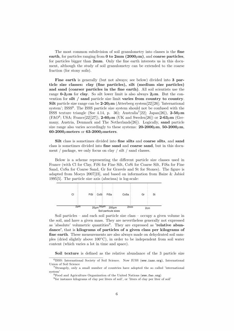

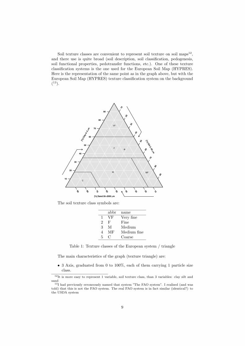


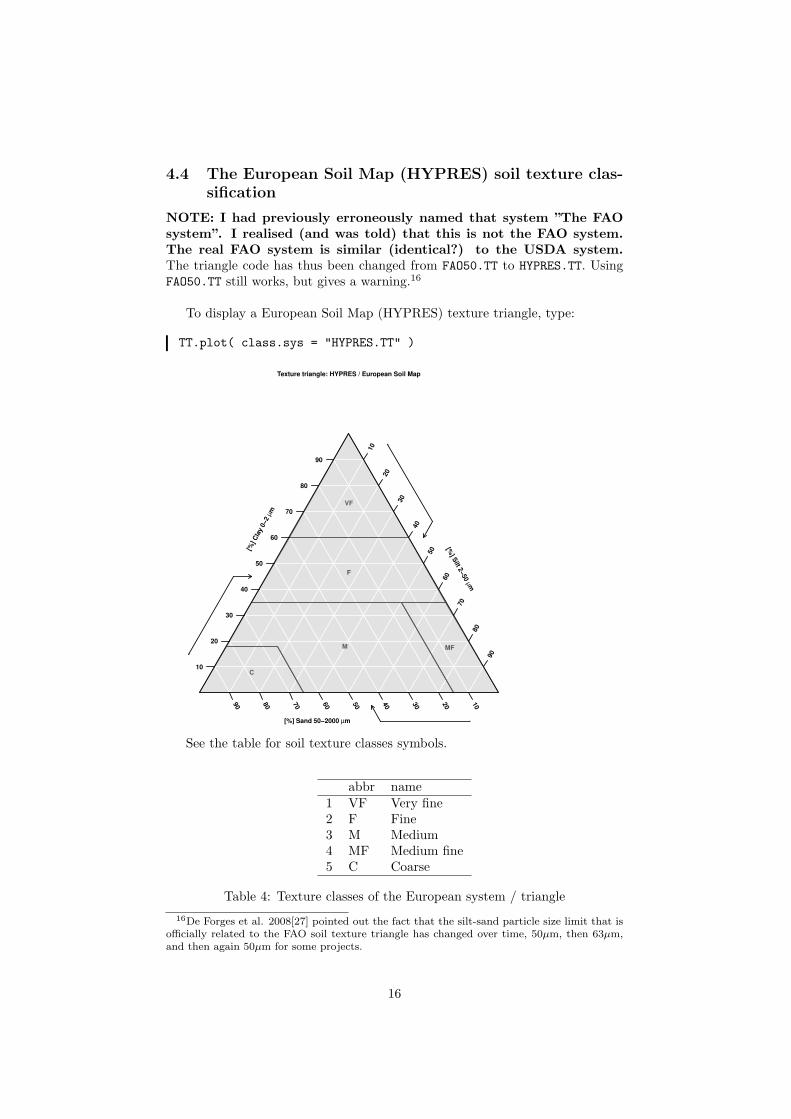


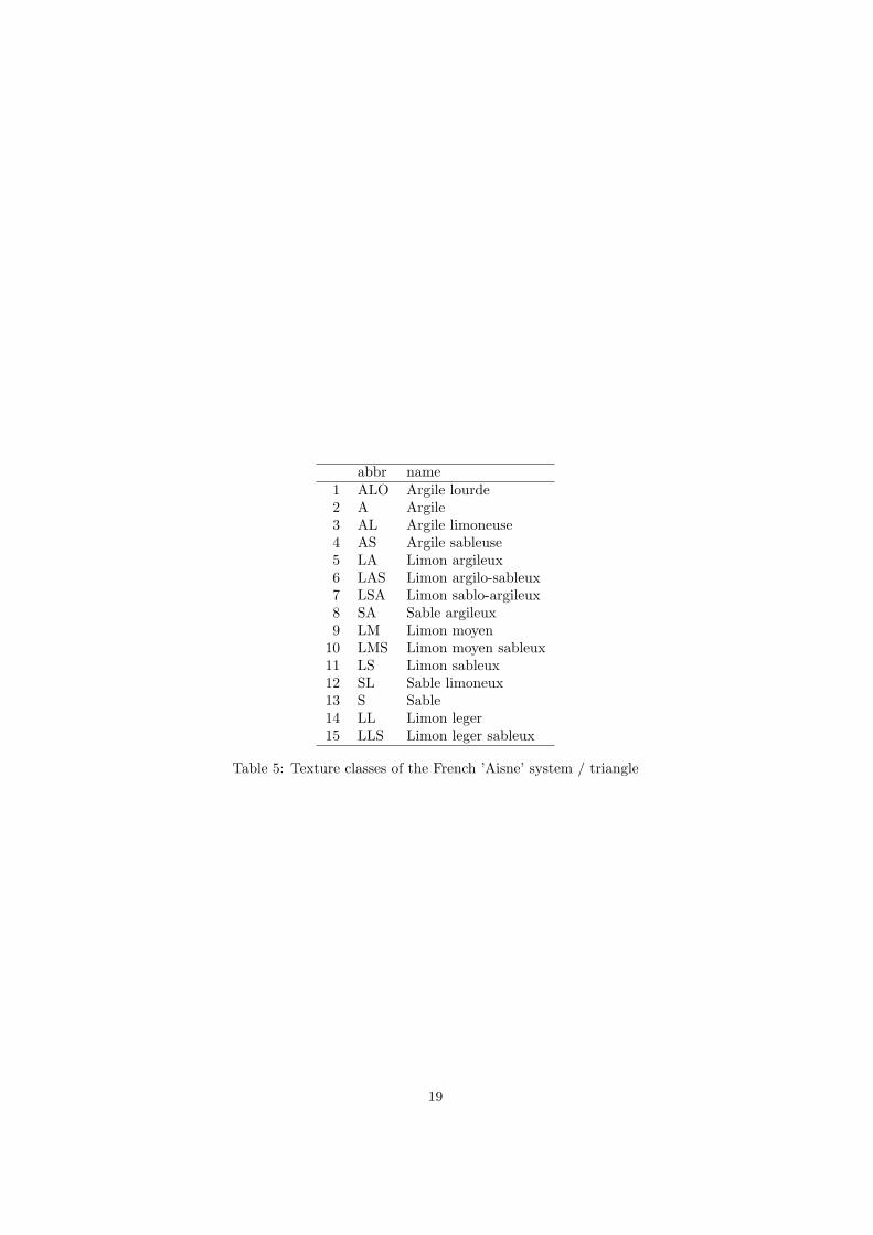

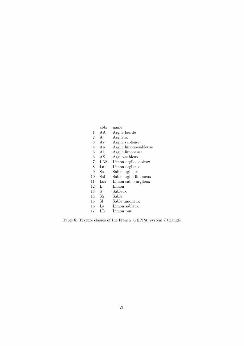
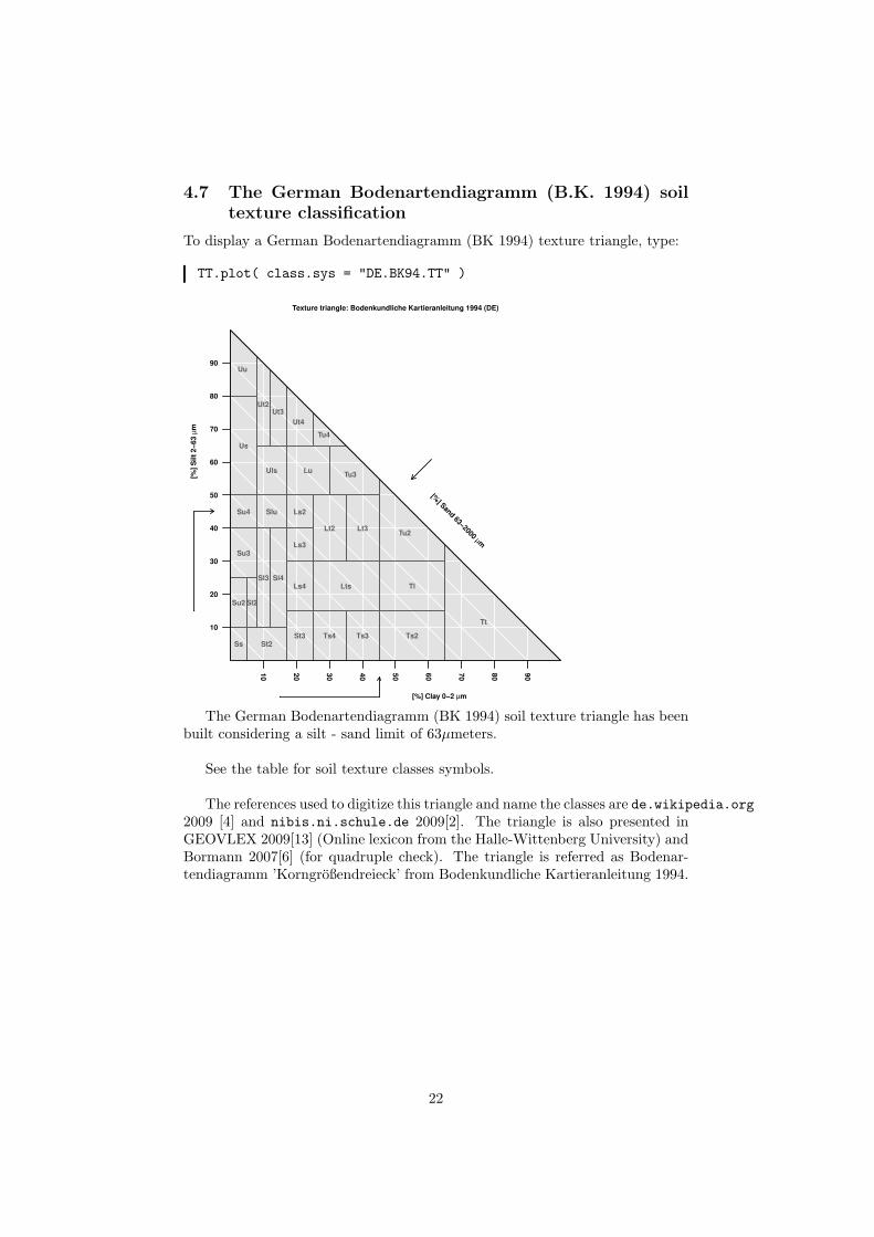


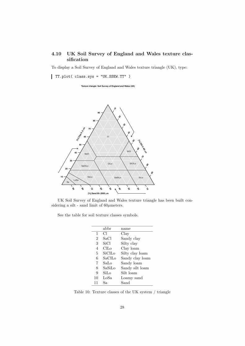
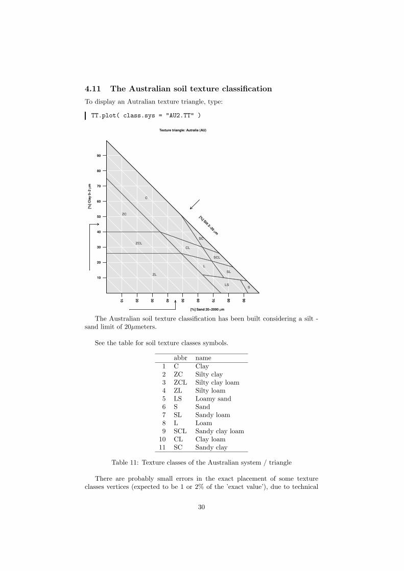


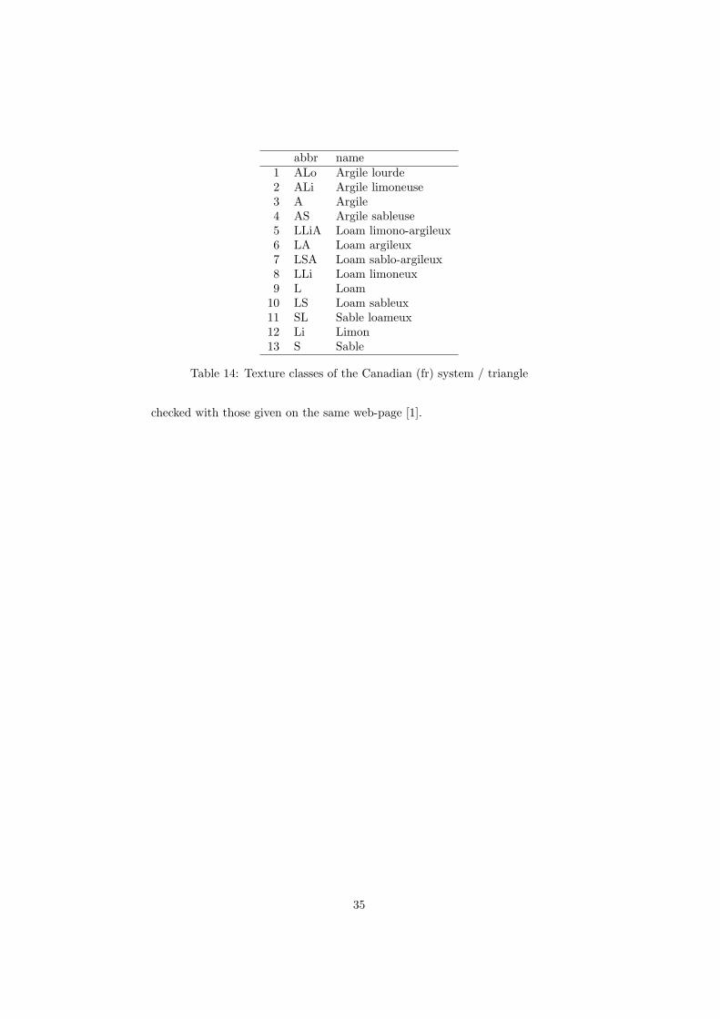


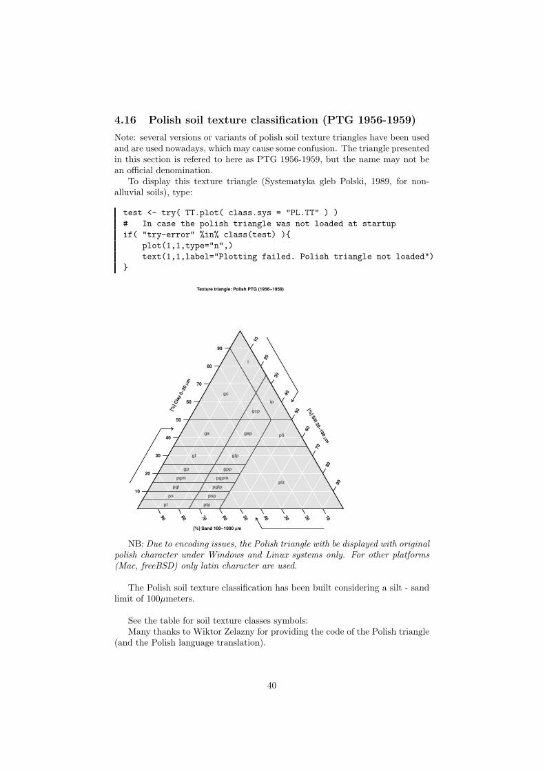

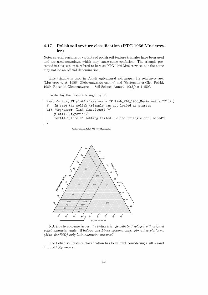


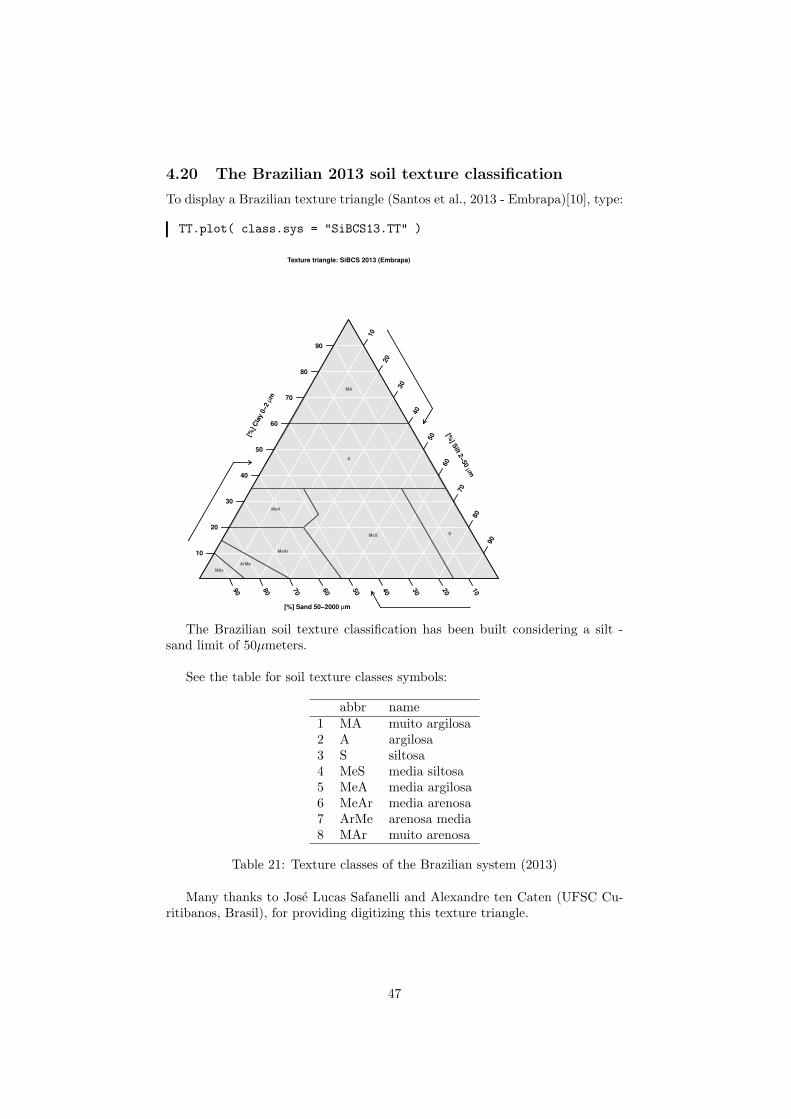

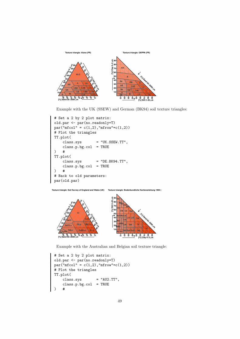


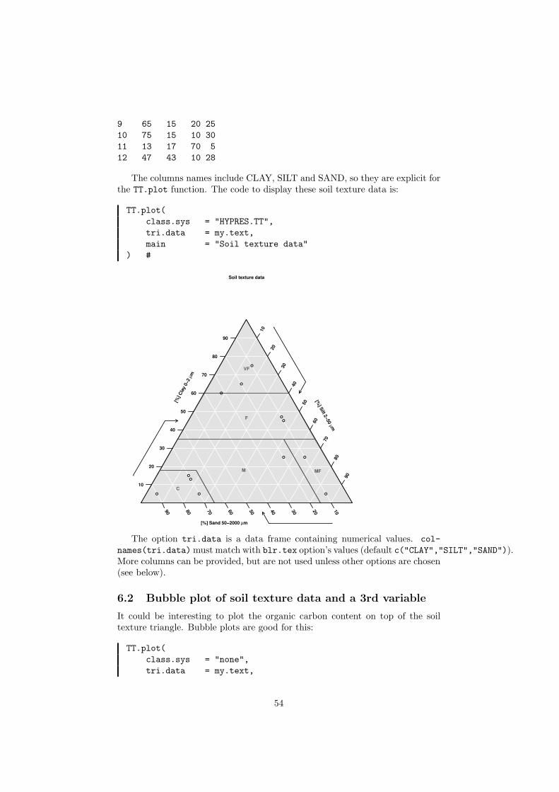


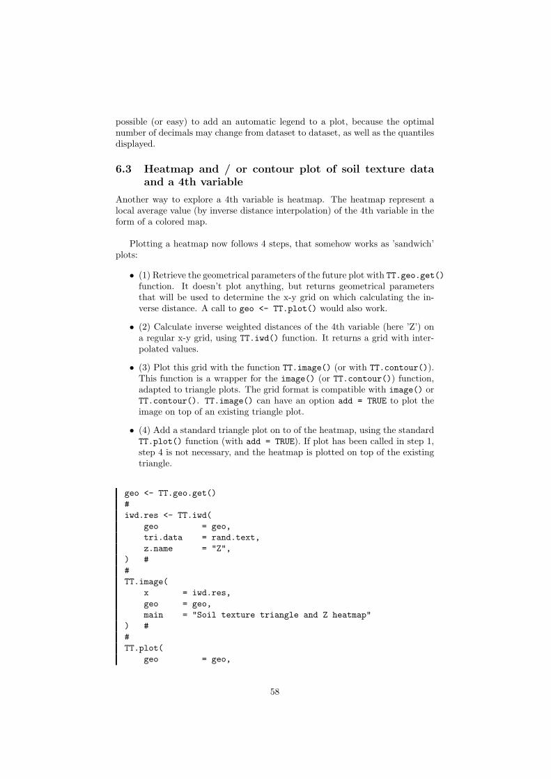


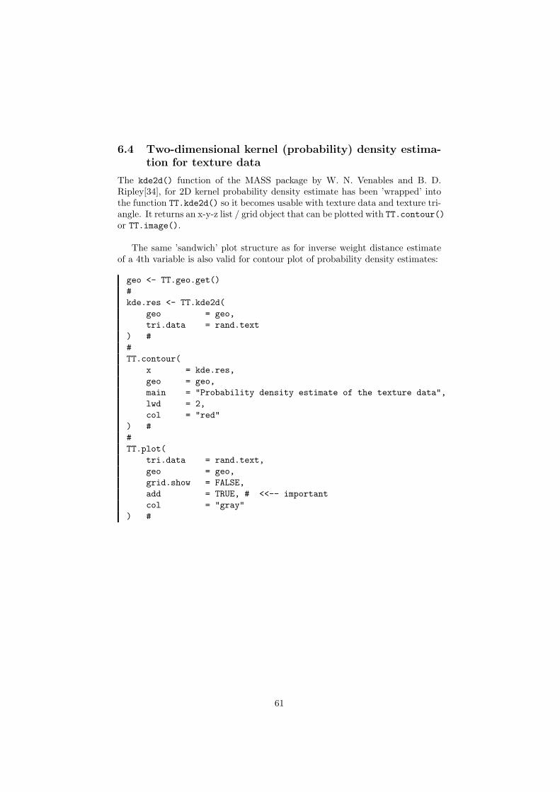


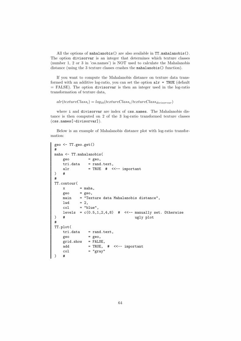


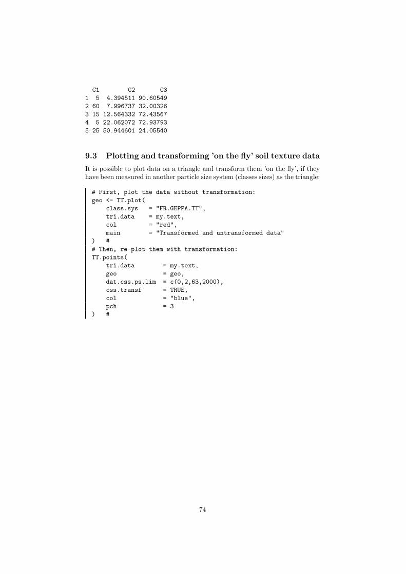


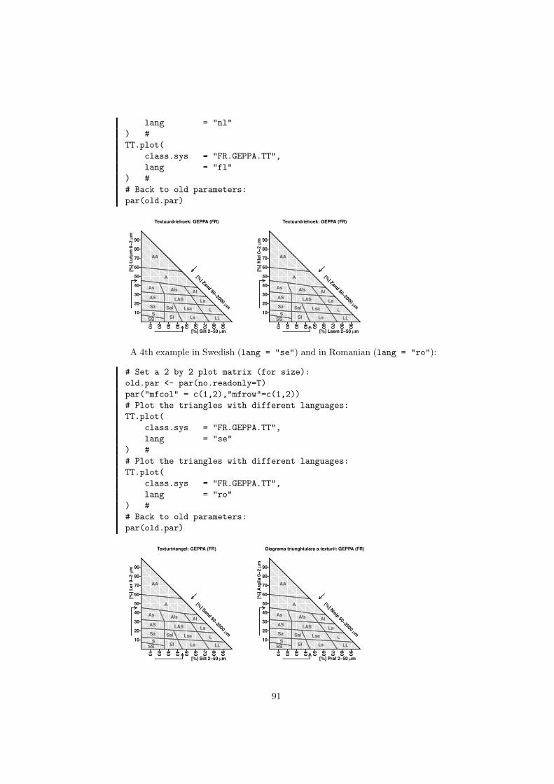

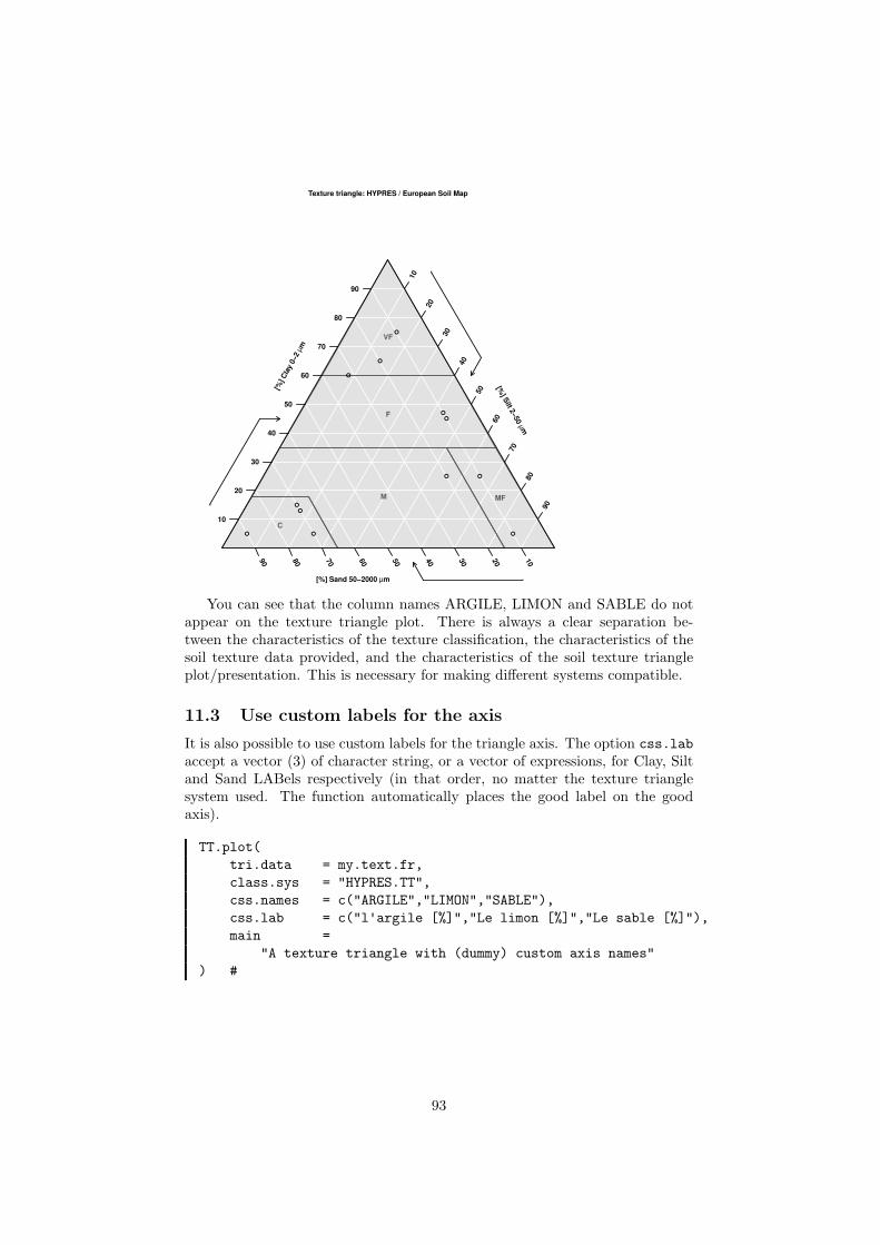

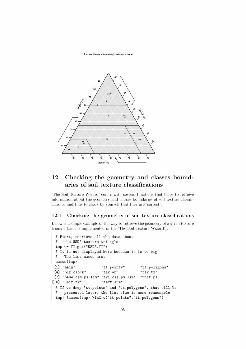


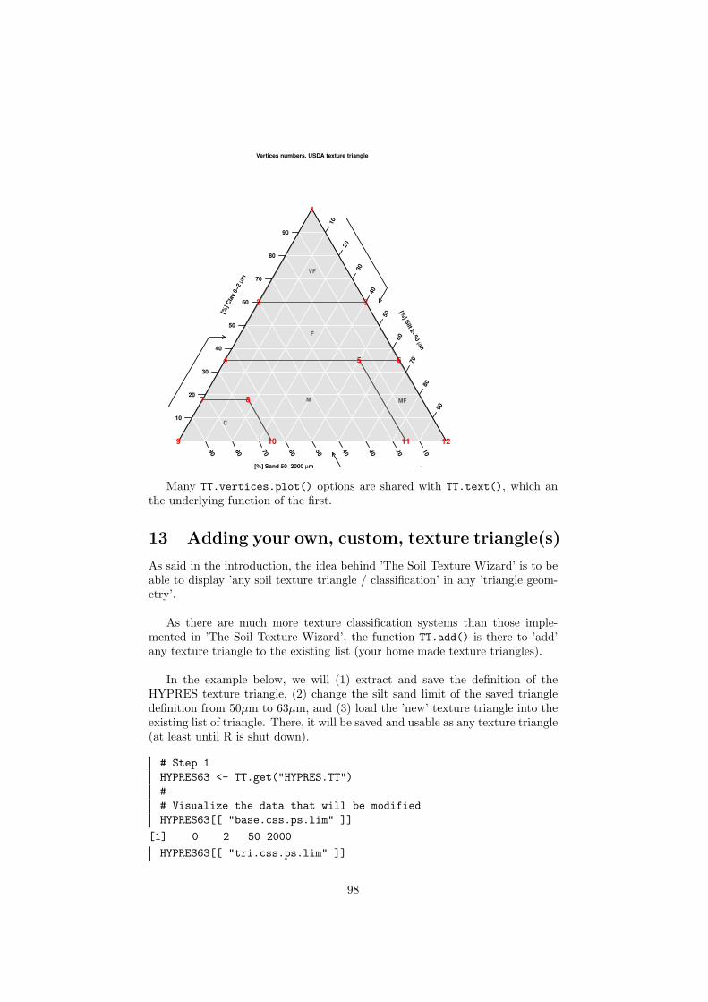


![Extended Gaussian-Filtered Local Binary Patterns for ......LBP[17] as a powerful texture descriptor has been widely applied to texture classification, face recognition [5], and medical](https://static.documents.pub/doc/80x56/6141d7882035ff3bc7624942/extended-gaussian-filtered-local-binary-patterns-for-lbp17-as-a-powerful.jpg)


![arXiv:1403.1687v1 [cs.CV] 7 Mar 2014Rigid-Motion Scattering for Texture Classification 3 periments are reproducible with the ScatNet (Scat-Net, 2013) MATLAB toolbox. 2 Invariance](https://static.documents.pub/doc/80x56/5f869dc4529519217c2216fd/arxiv14031687v1-cscv-7-mar-2014-rigid-motion-scattering-for-texture-classiication.jpg)


