Theta Functions, Old and New Arnaud Beauville * c Higher Education Press and International Press Beijing-Boston Open Problems and Surveys of Contemporary Mathematics SMM 6, pp. 99–131 Contents Introduction 100 1 The cohomology of a torus 101 1.1 Real tori ................................. 101 1.2 Complex tori .............................. 102 2 Line bundles on complex tori 103 2.1 The Picard group of a manifold .................... 103 2.2 Flat line bundles ............................ 104 2.3 Systems of multipliers ......................... 104 2.4 Interlude: hermitian forms ....................... 106 2.5 Systems of multipliers associated to hermitian forms ........ 106 2.6 The theorem of the square ....................... 108 3 Polarizations 109 3.1 Frobenius lemma ............................ 109 3.2 Polarizations and the period matrix ................. 110 3.3 The moduli space of p.p.a.v....................... 111 3.4 Theta functions ............................. 112 3.5 Comments ................................ 114 3.6 Reminder: line bundles and maps into projective space ....... 114 3.7 The Lefschetz theorem ......................... 115 3.8 The linear system |2Θ| ......................... 115 * Laboratoire J.-A. Dieudonn´ e , Universit´ e de Nice, Parc Valrose 06108, Nice cedex 2, France. Email: [email protected]
Theta functions are holomorphic functions on Cg , quasi-periodic with respect toa lattice. For g = 1 they have been introduced by Jacobi; in the general case theyhave been thoroughly studied by Riemann and his followers. From a modern pointof view they are sections of line bundles on certain complex tori; in particular, thetheta functions associated to an algebraic curve C are viewed as sections of anatural line bundle (and of its tensor powers) on a complex torus associated to C ,the Jacobian, which parametrizes topologically trivial line bundles on C .
Around 1980, under the impulsion of mathematical physics, the idea emergedgradually that one could replace in this definition line bundles by higher rankvector bundles. The resulting sections are called generalized (or non-abelian) thetafunctions ; they turn out to share some (but not all) of the beautiful properties ofclassical theta functions.
The goal of these lectures is to develop first the modern theory of classicaltheta functions (complex tori, line bundles, Jacobians), then to explain how it canbe generalized by considering higher rank vector bundles. We have tried to makethem accessible for students with a minimal background in complex geometry:Chapter 0 of [13] should be more than enough. At a few places, especially in thelast chapters, we had to use some more advanced results. Also we have not tried tobe exhaustive: sometimes we just give a sketch of proof, or we prove a particularcase, or we just admit the result.
These notes come from a series of lectures given at Tsinghua University inApril 2011. I am grateful to Tsinghua University and Professor S.-T. Yau for thegenerous invitation.
Theta Functions, Old and New 101
1 The cohomology of a torus
1.1 Real tori
Let V be a real vector space, of dimension n . A lattice in V is a Z-module Γ ⊂ Vsuch that the induced map Γ⊗ZR→ V is an isomorphism; equivalently, any basisof Γ over Z is a basis of V . In particular Γ ∼= Zn .
The quotient T := V/Γ is a smooth, compact Lie group, isomorphic to (S1)n .The quotient homomorphism π : V → V/Γ is the universal covering of T . ThusΓ is identified with the fundamental group π1(T ).
We want to consider the cohomology algebra H∗(T,C). We think of it asbeing de Rham cohomology: recall that a smooth p-form ω on T is closed ifdω = 0, exact if ω = dη for some (p − 1)-form η . Then
Hp(T,C) =closed p-forms
exact p-forms·
Let ℓ be a linear form on V . The 1-form dℓ on V is invariant by translation,hence is the pullback by π of a 1-form on T that we will still denote dℓ . Let(x1, . . . , xn) be a system of coordinates on V . The forms (dx1, . . . , dxn) form abasis of the cotangent space T ∗
a (T ) at each point a ∈ T ; thus a p-form ω on Tcan be written in a unique way
ω =∑
i1<···<ip
ωi1···ip(x) dxi1 ∧ · · · ∧ dxip
,
where the ωi1···ipare smooth functions on T (with complex values).
An important role in what follows will be played by the translations ta : x 7→x + a of T . We say that a p-form ω is constant if it is invariant by translation,that is, t∗aω = ω for all a ∈ T ; in terms of the above expression for ω , it meansthat the functions ωi1...ip
are constant. Such a form is determined by its valueat 0, which is a skew-symmetric p-linear form on V = T0(T ). We will denote byAltp(V,C) the space of such forms, and identify it to the space of constant p-forms.A constant form is closed, hence we have a linear map δp : Altp(V,C) → Hp(T,C).Note that Alt1(V,C) is simply HomR(V,C), and δ1 maps a linear form ℓ to theclass of dℓ .
Proposition 1.1. The map δp : Altp(V,C) → Hp(T,C) is an isomorphism.
Proof . There are various elementary proofs of this, see for instance [8], III.4. Tosave time we will use the Kunneth formula. We choose our coordinates (x1, . . . , xn)so that V = Rn , Γ = Zn . Then T = T1 × · · · × Tn , with Ti
∼= S1 for each i , anddxi is a 1-form on Ti , which generates H1(Ti,C). The Kunneth formula givesan isomorphism of graded algebras H∗(T,C) ∼−→
⊗
i H∗(Ti,C). This means thatH∗(T,C) is the exterior algebra on the vector space with basis (dx1, . . . , dxn),and this is equivalent to the assertion of the Proposition.
What about H∗(T,Z)? The Kunneth isomorphism shows that it is torsionfree, so it can be considered as a subgroup of H∗(T,C). By definition of the
102 Arnaud Beauville
de Rham isomorphism the image of Hp(T,Z) in Hp(T,C) is spanned by theclosed p-forms ω such that
∫
σ ω ∈ Z for each p-cycle σ in Hp(T,Z). Writeagain T = Rn/Zn ; the closed paths γi : t 7→ tei , for t ∈ [0, 1], form a basisof H1(T,Z), and we have
∫
γidℓ = ℓ(ei). Thus H1(T,Z) is identified with the
subgroup of H1(T,C) = HomR(V,C) consisting of linear forms V → C whichtake integral values on Γ; it is isomorphic to HomZ(Γ,Z). Applying again theKunneth formula gives:
Proposition 1.2. For each p , the image of Hp(T,Z) in Hp(T,C) ∼= Altp(V,C)is the subgroup of forms which take integral values on Γ ; it is isomorphic toAltp(Γ,Z) .
1.2 Complex tori
From now on we assume that V has a complex structure, that is, V is a complexvector space, of dimension g . Thus V ∼= Cg and Γ ∼= Z2g . Then T := V/Γ isa complex manifold, of dimension g , in fact a complex Lie group; the coveringmap π : V → V/Γ is holomorphic. We say that T is a complex torus. Beware:
while all real tori of dimension n are diffeomorphic to (S1)n , there are manynon-isomorphic complex tori of dimension g – more about that in Sect. 3.3 below.
The complex structure of V provides a natural decomposition
HomR(V,C) = V ∗ ⊕ V∗
,
where V ∗ := HomC(V,C) and V∗
= HomC(V ,C) are the subspaces of C-linearand C-antilinear forms respectively. We write the corresponding decompositionof H1(T,C)
H1(T,C) = H1,0(T ) ⊕ H0,1(T ) .
If (z1, . . . , zg) is a coordinate system on V , H1,0(T ) is the subspace spanned bythe classes of dz1, . . . , dzg , while H1,0(T ) is spanned by the classes of dz1, . . . , dzg .
The decomposition HomR(V,C) = V ∗ ⊕ V∗
gives rise to a decomposition
Altp(V,C) ∼= ∧pV ∗ ⊕ (∧p−1V ∗ ⊗ V∗) ⊕ · · · ⊕ ∧pV
∗
which we writeHp(T,C) = Hp,0(T ) ⊕ · · · ⊕ H0,p(T ) .
The forms in Altp(V,C) which belong to Hp,0(T ) (resp. H0,p(T )) are thosewhich are C-linear (resp. C-antilinear) in each variable. It is not immediate tocharacterize those which belong to Hq,r(T ) for q, r > 0; for p = 2 we have:
Proposition 1.3. Via the identification H2(T,C) = Alt2(V,C) , H2,0 is the spaceof C-bilinear forms, H0,2 the space of C-biantilinear forms, and H1,1 is the spaceof R-bilinear forms E such that E(ix, iy) = E(x, y) .
Proof . We have only to prove the last assertion. For ε ∈ ±1 , let Eε bethe space of forms E ∈ Alt2(V,C) satisfying E(ix, iy) = εE(x, y). We haveAlt2(V,C) = E1 ⊕ E−1 , and H2,0 and H0,2 are contained in E−1 .
hence H1,1 is contained in E1 ; it follows that H2,0 ⊕ H0,2 = E−1 and H1,1 =E1 .
2 Line bundles on complex tori
2.1 The Picard group of a manifold
Our next goal is to describe all holomorphic line bundles on our complex torus T .Recall that line bundles on a complex manifold M form a group, the Picard groupPic(M) (the group structure is given by the tensor product of line bundles). Itis canonically isomorphic to the first cohomology group H1(M, O∗
M ) of the sheafO∗
M of invertible holomorphic functions on M . To compute this group a standardtool is the exponential exact sequence of sheaves
0 → ZM → OMe
−→ O∗M → 1
where e(f) := exp(2πif), and ZM denotes the sheaf of locally constant functionson M with integral values. This gives a long exact sequence in cohomology
H1(M,Z) −→ H1(M, OM ) −→ Pic(M)c1−→ H2(M,Z) −→ H2(M, OM ) (2.1)
For L ∈ Pic(M), the class c1(L) ∈ H2(M,Z) is the first Chern class of L . Itis a topological invariant, which depends only on L as a topological complex linebundle (this is easily seen by replacing holomorphic functions by continuous onesin the exponential exact sequence).
When M is a projective (or compact Kahler) manifold, Hodge theory pro-vides more information on this exact sequence.1 The image of c1 is the kernelof the natural map H2(M,Z) → H2(M, OM ). This map is the composition ofthe maps H2(M,Z) → H2(M,C) → H2(M, OM ) deduced from the injections ofsheaves ZM → CM → OM . Now the map H2(M,C) → H2(M, OM ) ∼= H0,2 isthe projection onto the last summand of the Hodge decomposition
H2(M,C) = H2,0 ⊕ H1,1 ⊕ H0,2
(for the experts: this can be seen by comparing the de Rham complex with theDolbeault complex.)
Thus the image of c1 consists of classes α ∈ H2(M,Z) whose image αC =α0,2 + α1,1 + α0,2 in H2(M,C) satisfies α0,2 = 0. But since αC comes fromH2(M,R) we have α2,0 = α0,2 = 0: the image of c1 consists of the classes inH2(M,Z) whose image in H2(M,C) belongs to H1,1 (“Lefschetz theorem”).
1In this section and the following we use standard Hodge theory, as explained in [13], 0.6.Note that Hodge theory is much easier in the two cases of interest for us, namely complex toriand algebraic curves.
104 Arnaud Beauville
The kernel of c1 , denoted Pico(M), is the group of topologically trivialline bundles. The exact sequence (2.1) shows that it is isomorphic to the quo-tient of H1(M, OM ) by the image of H1(M,Z). We claim that this image isa lattice in H1(M, OM ) : this is equivalent to saying that the natural mapH1(M,R) → H1(M, OM ) is bijective. By Hodge theory, this map is identifiedwith the restriction to H1(M,R) of the projection of H1(M,C) = H1,0 ⊕ H0,1
onto H0,1 . Since H1(M,R) is the subspace of classes α+α in H1(M,C), the pro-jection H1(M,R) → H0,1 is indeed bijective. Thus Pico(M) is naturally identifiedwith the complex torus H1(M, OM )/H1(M,Z).
2.2 Flat line bundles
There is another description of Pico(M) which will be of interest for us. Insteadof holomorphic line bundles, defined by holomorphic transition functions, we canconsider flat line bundles, defined by locally constant transition functions; theyare parametrized by H1(M,C∗).
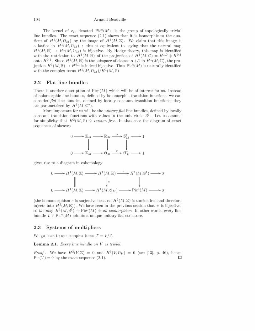
More important for us will be the unitary flat line bundles, defined by locallyconstant transition functions with values in the unit circle S1 . Let us assumefor simplicity that H2(M,Z) is torsion free. In that case the diagram of exactsequences of sheaves
0 // ZM//
RMe //
S1M
//
1
0 // ZM// OM
e // O∗M
// 1
gives rise to a diagram in cohomology
0 // H1(M,Z) // H1(M,R)ε //
π
H1(M, S1) //
0
0 // H1(M,Z) // H1(M, OM ) // Pico(M) // 0
(the homomorphism ε is surjective because H2(M,Z) is torsion free and thereforeinjects into H2(M,R)). We have seen in the previous section that π is bijective,so the map H1(M, S1) → Pico(M) is an isomorphism. In other words, every linebundle L ∈ Pico(M) admits a unique unitary flat structure.
2.3 Systems of multipliers
We go back to our complex torus T = V/Γ.
Lemma 2.1. Every line bundle on V is trivial.
Proof . We have H2(V,Z) = 0 and H1(V, OV ) = 0 (see [13], p. 46), hencePic(V ) = 0 by the exact sequence (2.1).
Theta Functions, Old and New 105
Let L be a line bundle on T . We consider the diagram
π∗L //
L
V
π // T
The action of Γ on V lifts to an action on π∗L = V ×T L . We know that π∗L istrivial; we choose a trivialization π∗L ∼−→ V × C . We obtain an action of Γ onV ×C , so that L is the quotient of V ×C by this action. An element γ of Γ actslinearly on the fibers, hence by
γ · (z, t) = (z + γ, eγ(z) t) for z ∈ V, t ∈ C
where eγ is a holomorphic invertible function on V . This formula defines a groupaction of Γ on V × C if and only if the functions eγ satisfy
eγ+δ(z) = eγ(z + δ) eδ(z) (“cocycle condition”).
A family (eγ)γ∈Γ of holomorphic invertible functions on V satisfying thiscondition is called a system of multipliers. Every line bundle on T is defined bysuch a system.
A theta function for the system (eγ)γ∈Γ is a holomorphic function V → C
satisfyingθ(z + γ) = eγ(z)θ(z) for all γ ∈ Γ, z ∈ V .
Proposition 2.2. Let (eγ)γ∈Γ be a system of multipliers, and L the associatedline bundle. The space H0(T, L) is canonically identified with the space of thetafunctions for (eγ)γ∈Γ .
Proof . Any global section s of L lifts to a section s = π∗s of π∗L = V ×T Lover V , defined by s(z) = (z, s(πz)); it is Γ-invariant in the sense that s(z +γ) =γ · s(z). Conversely, a Γ-invariant section of π∗L comes from a section of L .Now a section of π∗L ∼= V × C is of the form z 7→ (z, θ(z)), where θ : V → C isholomorphic. It is Γ-invariant if and only if θ is a theta function for (eγ)γ∈Γ .
Let (eγ)γ∈Γ and (e′γ)γ∈Γ be two systems of multipliers, defining line bundlesL and L′ . The line bundle L ⊗ L′ is the quotient of the trivial line bundleV × (C⊗C) by the tensor product action γ · (z, t⊗ t′) = (z + γ, eγ(z) t⊗ e′γ(z) t′);therefore it is defined by the system of multipliers (eγe′γ)γ∈Γ . In other words,multiplication defines a group structure on the set of systems of multipliers, andwe have a surjective group homomorphism
systems of multipliers −→ Pic(T ) .
A system of multipliers (eγ)γ∈Γ lies in the kernel if and only if the associatedline bundle admits a section which is everywhere 6= 0; in view of Proposition2.2, this means that there exists a holomorphic function h : V → C∗ such that
eγ(z) =h(z + γ)
h(z). We will call such systems of multipliers trivial. Thus we
can always multiply a given system (eγ) by a trivial one without changing theassociated line bundle.
106 Arnaud Beauville
Remark 2.3. (only for the readers who know group cohomology) Put H∗ :=H0(V, O∗
V ). The system of multipliers are exactly the 1-cocycles of Γ with valuesin H∗ , and the trivial systems are the coboundaries. Thus we get a group isomor-phism H1(Γ, H∗) ∼−→ Pic(T ) (see [20], §2 for a more conceptual explanation ofthis isomorphism).
Remark 2.4. The argument in this section apply equally well to flat line bundles,since obviously H1(V,C∗) = 0. The corresponding systems of multipliers are ofthe form a(γ)γ∈Γ , where a : Γ → C∗ is a homomorphism. Similarly, unitaryflat line bundles correspond to homomorphisms Γ → S1 . This is nothing but theclassical isomorphism H1(T, A) ∼−→ Hom(π1(T ), A) for A = C∗ or S1 .
2.4 Interlude: hermitian forms
There are many holomorphic invertible functions on V , hence many systems ofmultipliers giving rise to the same line bundle. Our next goal will be to finda subset of such systems such that each line bundle corresponds exactly to onesystem of multipliers in that subset. This will involve hermitian forms on V , solet us fix our conventions.
A hermitian form H on V will be C-linear in the second variable, C-antilinear in the first. We put S(x, y) = Re H(x, y) and E(x, y) = Im H(x, y). Sand E are R-bilinear forms on V , S is symmetric, E is skew-symmetric; theysatisfy:
Using these relations one checks easily that the following data are equivalent:
• The hermitian form H ;• The symmetric R-bilinear form S with S(x, y) = S(ix, iy);• The skew-symmetric R-bilinear form E with E(x, y) = E(ix, iy).
Moreover,H non-degenerate ⇐⇒ E non-degenerate ⇐⇒ S non-degenerate.
2.5 Systems of multipliers associated to hermitian forms
We denote by P the set of pairs (H, α), where H is a hermitian form on V , α amap from Γ to S1 , satisfying:
E := Im(H) takes integral values on Γ, and α satisfies
α(γ + δ) = α(γ)α(δ)(−1)E(γ,δ) .
The law (H, α) · (H ′, α′) = (H + H ′, α α′) defines a group structure on P .For (H, α) ∈ P , we put
eγ(z) = α(γ)eπ[H(γ,z)+ 12H(γ,γ)] .
Theta Functions, Old and New 107
We leave as an (easy) exercise to check that this defines a system of multipliers.The corresponding line bundle will be denoted L(H, α). The map (H, α) 7→L(H, α) from P onto Pic(T ) is a group homomorphism; we want to prove that itis an isomorphism.
Proposition 2.5. The first Chern class c1(L(H, α)) is equal to E ∈ Alt2(Γ,Z) ∼=H2(T,Z) .
Proof . We will use Chern’s original definition of the first Chern class of a linebundle L on a compact manifold M (see [13], p. 141). One chooses a C∞ metrich on L ; this is nothing but a C
∞ function L → R+ , which is positive outsidethe zero section and satisfies h(λx) = |λ|2h(x) for x ∈ L , λ ∈ C . If s is a localnon-vanishing holomorphic section of L , the 2-form ωL,h := 1
2πi∂∂ log h(s) doesnot depend on the choice of s ; thus ωL,h is a globally defined closed 2-form, whoseclass in H2(M,C) represents c1(L).
To apply this in our situation, we observe that the metric h on V ×C definedby h(z, t) = e−πH(z,z)|t|2 is invariant under Γ; hence it is the pullback of a metrich on L(H, α). The form π∗ωL,h is equal to ωV ×C,h ; to compute it we apply ourformula to the section s : z 7→ (z, 1) of V × C . We find
ωV ×C,h =1
2πi∂∂ log e−πH(z,z) =
i
2∂∂ H(z, z) .
It remains to prove that i2∂∂ H(z, z) is the constant 2-form defined by E .
It suffices to prove this when H(x, y) = xjyj ; then i2∂∂ H(z, z) = i
2dzj ∧dzj . Letv = (v1, . . . , vg), w = (w1, . . . , wg) two vectors of V ; we have
(See [20], §2 for a proof in terms of group cohomology.)
Theorem 2.6. The map (H, α) 7→ L(H, α) defines a group isomorphism P∼−→
Pic(T ) .
Proof . Let Q be the group of hermitian forms H on V such that Im(H) is integralon Γ. By Proposition 2.5 and Section 2.1 we have a commutative diagram
0 // Hom(Γ, S1) //
Lo
P //
L
Q //
ι
0
0 // Pico(T ) // Pic(T )c1 // H2(T,Z)
with ι(H) = Im(H) ∈ Alt2(Γ,Z) ∼= H2(T,Z).Let us first prove that ι is bijective onto Im(c1). Let E ∈ Alt2(Γ,Z) ∼=
H2(T,Z); we have seen in Section 2.1 that E belongs to Im(c1) if and only if itbelongs to H1,1 , that is satisfies E(ix, iy) = E(x, y) (Proposition 1.3). By Section
108 Arnaud Beauville
2.4 this is equivalent to E = Im(H) for a hermitian form H ∈ Q ; moreover H isuniquely determined by E , hence our assertion.
The map Lo associates to a unitary character α : Γ → S1 the unitary flatbundle L(0, α); we have already seen that it is bijective (Section 2.2 and Remark2.4). Thus the map (H, α) 7→ L(H, α) is bijective.
2.6 The theorem of the square
This section is devoted to an important result, Theorem 2.8 below, which is ac-tually an easy consequence of our description of line bundles on T (we encouragethe reader to have a look at the much more elaborate proof in [20], §6, valid overany algebraically closed field).
Lemma 2.7. Let a ∈ V . We have t∗π(a)L(H, α) = L(H, α′) with α′(γ) =
α(γ)e(E(γ, a) .
Proof . In general, let L be a line bundle on T defined by a system of multipliers(eγ)γ∈Γ . Then (eγ(z + a))γ∈Γ is a system of multipliers, defining a line bundleL′ ; the self-map (z, t) 7→ (z + a, t) of V ×C is equivariant w.r.t. the actions of Γdefined by (eγ(z + a)) on the source and (eγ(z)) on the target, so it induces anisomorphism L′ ∼−→ t∗π(a)L .
We apply this to the multiplier eγ(z) = a(γ)eπ[H(γ,z)+ 12H(γ,γ)] ; we find eγ(z+
a) = eγ(z) eπH(γ,a) . Recall that we are free to multiply eγ(z) by h(z+γ)h(z) for
some holomorphic invertible function h ; taking h(z) = e−πH(a,z) , our multiplierbecomes eγ eπ[H(γ,a)−H(a,γ)] = eγ e2πiE(γ,a) .
Theorem 2.8 (Theorem of the square). Let L be a line bundle on T .1) The map
λL : T → Pico(T ), λL(a) = t∗aL ⊗ L−1
is a group homomorphism.
2) Let E ∈ Alt2(Γ,Z) be the first Chern class of L . We have
KerλL = Γ⊥/Γ , with Γ⊥ := z ∈ V | E(z, γ) ∈ Z for all γ ∈ Γ .
3) If E is non-degenerate, λL is surjective and has finite kernel.
4) If E is unimodular, λL is a group isomorphism.
Proof . By the Lemma, λL is the composition
Tε
−→ Hom(Γ, S1)Lo
−→ Pico(T ) ,
where ε(a), for a = π(a) ∈ T , is the map γ 7→ e(E(γ, a), and Lo is the iso-morphism α 7→ L(0, α) (Theorem 2.6). Therefore we can replace λL by ε in theproof. Then 1) and 2) become obvious.
Theta Functions, Old and New 109
Assume that E is non-degenerate. Let χ ∈ Hom(Γ, S1). Since Γ is a freeZ-module, we can find a homomorphism u : Γ → R such that χ(γ) = e(u(γ)) foreach γ ∈ Γ. Extend u to a R-linear form V → R ; since E is non-degenerate,there exists a ∈ V such that u(z) = E(z, a), hence ε(π(a)) = χ . Thus ε issurjective.
Let us denote by e : V → HomR(V,R) the R-linear isomorphism associatedto E . The dual Γ∗ := HomZ(Γ,Z) embeds naturally in HomR(V,R), and Γ⊥ isby definition e−1(Γ∗); then e identifies Γ⊥ with Γ∗ , so that the inclusion Γ ⊂ Γ⊥
corresponds to the map Γ → Γ∗ associated to E|Γ . This map has finite cokernel,and it is bijective if E is unimodular; this achieves the proof.
Remark 2.9. We have seen in Section 2.1 that Pico(T ) has a natural structureof complex torus; it is not difficult to prove that the map λL is holomorphic. Inparticular, when E is unimodular, λL is an isomorphism of complex tori.
Corollary 2.10. Assume that c1(L) is non-degenerate. Any line bundle L′ withc1(L
′) = c1(L) is isomorphic to t∗aL for some a in T .
Proof . L′ ⊗ L−1 belongs to Pico(T ), hence is isomorphic to t∗aL ⊗ L−1 for somea in T by 3).
The following immediate consequence of 1) will be very useful:
Corollary 2.11. Let a1, . . . , ar in T with∑
ai = 0 . Then t∗a1L ⊗ · · · ⊗ t∗ar
L ∼=L⊗r .
3 Polarizations
In this section we will consider a line bundle L = L(H, α) on our complex torusT such that the hermitian form H is positive definite. We will first look for aconcrete expression of the situation using an appropriate basis.
3.1 Frobenius lemma
The following easy result goes back to Frobenius:
Proposition 3.1. Let Γ be a free finitely generated Z-module, and E : Γ ×Γ → Z a skew-symmetric, non-degenerate form. There exists positive integersd1, . . . , dg with d1 | d2 | · · · | dg and a basis (γ1, . . . , γg; δ1, . . . , δg) of Γ such that
the matrix of E in this basis is
(
0 d
−d 0
)
, where d is the diagonal matrix with
entries (d1, . . . , dg) .
As a consequence we see that the determinant of E is the square of the integerd1 · · · dg , called the Pfaffian of E and denoted Pf(E). The most important casefor us will be when d1 = · · · = dg = 1, or equivalently det(E) = 1; in that caseone says that E is unimodular, and that (γ1, . . . , γg; δ1, . . . , δg) is a symplecticbasis of Γ.
ab
Note
Marked définie par ab
110 Arnaud Beauville
Proof . Let d1 be the minimum of the numbers E(α, β) for α, β ∈ Γ, E(α, β) > 0;choose γ, δ such that E(γ, δ) = d1 . For any ε ∈ Γ, E(γ, ε) is divisible by d1
– otherwise using Euclidean division we would find ε with 0 < E(γ, ε) < d1 .Likewise E(δ, ε) is divisible by d1 . Put U = Zγ⊕Zδ ; we claim that Γ = U ⊕U⊥ .Indeed, for x ∈ Γ, we have
x =E(x, δ)
d1γ +
E(γ, x)
d1δ + (x −
E(x, δ)
d1γ −
E(γ, x)
d1δ) .
Reasoning by induction on the rank of Γ, we find integers d2 | d3 | · · · | dg and a
basis (γ, γ2, . . . , γg; δ, δ2, . . . , δg) of Γ, such that the matrix of E is
(
0 d
−d 0
)
. It
remains to prove that d1 divides d2 ; otherwise, using Euclidean division again,we can find k ∈ Z such that 0 < E(γ + γ2, kδ + δ2) < d1 , a contradiction.
3.2 Polarizations and the period matrix
Going back to our complex torus T = V/Γ, we assume given a positive definitehermitian form H on V , such that E := Im(H) takes integral values on Γ. Sucha form is called a polarization of T ; if E is unimodular, we say that H is aprincipal polarization. A complex torus which admits a polarization is classicallycalled a (polarized) abelian variety; we will see below that it is actually a projectivemanifold. It is common to use the abbreviation p.p.a.v. for “principally polarizedabelian variety”.
We choose a basis (γ1, . . . , γg; δ1, . . . , δg) as in Proposition 3.1 (note that Eis non-degenerate by Section 2.4); we put γ′
j :=γj
djfor j = 1, . . . , g .
Lemma 3.2. (γ′1, . . . , γ
′g) is a basis of V over C .
Proof . Let W = Rγ′1 ⊕ · · · ⊕ Rγ′
g . Our statement is equivalent to V = W ⊕ iW .But if x ∈ W ∩ iW , we have H(x, x) = E(x, ix) = 0 since E|W = 0, hencex = 0.
Expressing the δj ’s in this basis gives a matrix τ ∈ Mg(C) with δj =∑
i τijγ′i . In the corresponding coordinates, we have
Γ = dZg ⊕ τZg
in other words, the elements of Γ are the column vectors dp + τq with p, q ∈ Zg .The matrix τ is often called the period matrix.
Note that in case the polarization is principal we have γ′i = γi and Γ =
Zg ⊕ τZg .
Proposition 3.3. The matrix τ is symmetric, and Im(τ) is positive definite.
Proof . Put τ = A + iB , with A, B ∈ Mg(R). We will compare the bases(γ1, . . . , γg; δ1, . . . , δg) and (γ′
1, . . . , γ′g; iγ
′1, . . . , iγ
′g) of V over R . The change of
Theta Functions, Old and New 111
basis matrix (expressing the vectors of the first basis in the second one) is P =(
d A0 B
)
. Therefore the matrix of E in the second basis is
tP−1
(
0 d
−d 0
)
P−1 =
(
0 B−1
−tB−1 tB−1(A − tA)B−1
)
Now the condition E(ix, iy) = E(x, y), expressed in the basis (γ′1, . . . , γ
′g;
iγ′1, . . . , iγ
′g), is equivalent to A = tA and B = tB ; we have H(γ′
j , γ′k) = E(γ′
j , iγ′k),
so the matrix of H in the basis (γ′1, . . . , γ
′g) (over C) is B−1 , and the positivity
of H is equivalent to that of B .
3.3 The moduli space of p.p.a.v.
In this section we restrict for simplicity to the case the polarization is principal ; weencourage the reader to adapt the argument to the general case (see for instance[8], VII.1).
We have seen that the choice of a symplectic basis determines the matrixτ , which in turn completely determines T and H : we have V = Cg and Γ =Γτ := Zg ⊕ τZg ; the hermitian form H is given by the matrix Im(τ)−1 , and itsimaginary part E by E(p + τq, p′ + τq′) = tpq′ − tqp′ .
The space of symmetric matrices τ ∈ Mg(C) with Im(τ) positive definite isdenoted Hg , and called the Siegel upper half space. It is an open subset of thevector space of complex symmetric matrices. From what we have seen it followsthat Hg parametrizes p.p.a.v. (V/Γ, H) endowed with a symplectic basis of thelattice Γ.
Now we want to get rid of the choice of the symplectic basis. We haveassociated to a symplectic basis an isomorphism V ∼−→ Cg which maps Γ to thelattice Γτ . A change of the basis amounts to a linear automorphism M of Cg ,inducing a symplectic isomorphism Γτ
∼−→ Γτ ′ . Such an isomorphism is given
by
(
p′
q′
)
= P
(
pq
)
, where P belongs to the symplectic group Sp(2g,Z), that is,
Thus the group Sp(2g,Z) acts on Hg by (P, τ) 7→ (aτ − b)(−cτ + d)−1 , and twomatrices τ, τ ′ correspond to the same p.p.a.v. with different symplectic bases iff
112 Arnaud Beauville
they are conjugated under this action. To get a nicer formula, we observe that
(
a −b−c d
)
= tP t , with t =
(
1 00 −1
)
;
since tJt = −J , the map P 7→ tP t is an automorphism of Sp(2g,Z). Composingour action with this automorphism, we obtain:
Proposition 3.4. The group Sp(2g,Z) acts on Hg by
(
a bc d
)
· τ = (aτ + b)
(cτ + d)−1 . The quotient Ag := Hg/Sp(2g,Z) parametrizes isomorphism classesof g -dimensional p.p.a.v.
It is not difficult to show that the action of Sp(2g,Z) on Hg is nice (“properlydiscontinuous”), so that Ag is an analytic space ([8], VII.1). A much more subtleresult is that Ag is Zariski open in a projective variety, the Satake compactificationAg .
We have not made precise in which sense Ag parametrizes p.p.a.v. It isactually what is called a moduli space; we will give a precise definition in the caseof vector bundles (see Section 4.2 below), which can be adapted without difficultyto this case.
3.4 Theta functions
Let H be a polarization on T ; we keep the notation of the previous sections. Letα : Γ → S1 be any map satisfying α(γ + δ) = α(γ)α(δ)(−1)E(γ,δ) .
Proof . We first treat the case d1 = · · · = dg = 1. According to Prop. 2.2, we arelooking for theta functions satisfying
θ(z + γ) = α(γ)eπ[H(γ,z)+ 12 H(γ,γ)]θ(z) .
Recall that we are free to multiply eγ(z) by h(z+γ)h(z) for some h ∈ H0(V, O∗
V ) (this
amounts to multiply θ by h). We will use this to make θ periodic with respectto the basis elements γ1, . . . , γg of Γ.
As before we put W = Rγ1 ⊕ · · · ⊕ Rγg . Since E|W = 0, the form H|W is areal symmetric form; since V = W ⊕ iW (Lemma 3.2), it extends as a C-bilinearsymmetric form B on V . We put h(z) = e−
π2 B(z,z) : this amounts to replace H
in eγ(z) by H ′ := H − B . We have
Lemma 3.6. H ′(p + τq, z) = −2i tqz .
Proof . Let w ∈ W . We have H ′(w, y) = 0 for y ∈ W , hence also for anyy ∈ V because H ′ is C-linear in y . On the other hand for z ∈ V we haveH ′(z, w) = (H−B)(z, w) = (H−B)(w, z) = (H−H)(w, z) = 2iE(z, w). Thus forz =
∑
ziγi ∈ V we have H ′(γj , z) = 0 and H ′(δj , z) =∑
k zkH ′(δj , γk) = −2izj ,hence the lemma.
Theta Functions, Old and New 113
Put L = L(H, α). By Cor. 2.10, changing α amounts to replace L byt∗aL for some a ∈ T . Since the pullback map t∗a : H0(T, L) → H0(T, t∗aL) is anisomorphism, it suffices to prove the theorem for a particular value of α ; we chooseα(p + τq) = (−1)
Thus our theta functions must satisfy the quasi-periodicity condition
θ(z + p + τq) = θ(z) e(−tqz −1
2tqτq) for z ∈ Cg, p, q ∈ Zg .
In particular, they are periodic with respect to the subgroup Zg ⊂ Cg . This im-plies that they admit a Fourier expansion of the form θ(z) =
∑
m∈Zg c(m)e(tmz).Now let us express the quasi-periodicity condition; we have:
θ(z + p + τq) =∑
m∈Zg
c(m)e(tmτq)e(tmz)
and
θ(z)e(−tqz −1
2tqτq) =
∑
m∈Zg
c(m)e(t(m − q)z −1
2tqτq)
=∑
m∈Zg
c(m + q)e(−1
2tqτq)e(tmz) .
Comparing we find c(m + q) = c(m)e(t(m + q2 )τq). Taking m = 0 gives c(q) =
c(0) e(12
tqτq). Thus our theta functions, if they exist, are all proportional to
θ(z) =∑
m∈Zg
e(tmz +1
2tmτm) .
It remains to prove that this function indeed exists, that is that the series con-verges. But the coefficients c(m) of the Fourier series satisfy |c(m)| = e−q(m) ,where q is a positive definite quadratic form, and therefore they decrease very fastas m → ∞ .
Now we treat the case d1 = · · · = dg = d . In this case the form 1dH is
a principal polarization, so we can take L = L⊗d0 , where L0 is the line bundle
considered above. The corresponding theta functions satisfy
θ(z + p + τq) = θ(z)e(−dtqz −d
2tqτq)
for z ∈ Cg, p, q ∈ Zg (“theta functions of order d”).
We write again θ(z) =∑
m∈Zg c(m)e(tmz); the quasi-periodicity condition gives
c(m + dq) = c(m)e(t(m +d
2)τq) = c(m)e(−1
dtmτm)e( 1
2dt(m + dq)τ(m + dq))
114 Arnaud Beauville
This determines up to a constant all coefficients c(m) for m in a given cosetε of Zg modulo dZg ; the corresponding theta function is
θ[ε](z) =∑
m∈ε
e(tmz +1
2dtmτm) . (3.1)
By what we have seen the functions θ[ε] , where ε runs through Zg/dZg , form abasis of the space of theta functions of order d ; in particular, the dimension ofthis space is dg .
The proof of the general case is completely analogous but requires morecomplicated notations. We will not need it in these lectures, so we leave it as anexercise for the reader.
3.5 Comments
The proof of the theorem gives much more than the dimension of the space of thetafunctions, namely an explicit basis (θ[ε])ε∈Zg/dZg of this space given by formula(3.1). In particular, when the polarization H is principal, the line bundles L(H, α)have a unique non-zero section (up to a scalar); the divisor of this section is calleda theta divisor of the p.p.a.v. (T, H). By Corollary 2.10 it is well-defined upto translation, so one speaks sometimes of “the” theta divisor. The choice of asymplectic basis gives a particular theta divisor Θτ , defined by the celebratedRiemann theta function
θ(z) =∑
m∈Zg
e(tmz +1
2tmτm) .
It is quite remarkable that starting from a linear algebra data (a lattice Γ inV and a polarization), we get a hypersurface Θ ⊂ T = V/Γ. When the p.p.a.v.comes from a geometric construction (Jacobians, Prym varieties, intermediate Ja-cobians), this divisor has a rich geometry, which reflects the objects we startedwith. In particular it is often possible to recover these objects from the data (T, Θ)(“Torelli theorem”), or to characterize the p.p.a.v. obtained in this way (“Schottkyproblem”).
3.6 Reminder: line bundles and maps into projective space
Let M be a projective variety, and L a line bundle on M . The linear system |L|is by definition P(H0(M, L)). Sending a nonzero section to its divisors identifies|L| with the set of effective divisors E on M such that OM (E) ∼= L .
The base locus B(L) of L is the intersection of the divisors in |L| . Assumethat L has no base point, that is, B(L) = ∅ . Then the divisors of |L| passingthrough a point m ∈ M form a hyperplane in |L| , corresponding to a point ϕL(m)in the dual projective space |L|∗ . This defines a morphism ϕL : M → |L|∗ .Choosing a basis (s0, . . . , sn) of H0(M, L) identifies |L| , hence also its dual |L|∗ ,to Pn ; then ϕL(m) = (s0(m), . . . , sn(m)), where we have fixed an isomorphismLm
∼−→ C to evaluate the si at m .
Theta Functions, Old and New 115
If E ∈ |L| , we also denote the linear system |L| by |E| , and the map ϕL byϕE . Thus |E| is the set of effective divisors linearly equivalent to E .
3.7 The Lefschetz theorem
Theorem 3.7 (Lefschetz). Let L be a line bundle on T .1) Assume H0(T, L) 6= 0 . For k ≥ 2 , the linear system |L⊗k| has no base
points.2) Assume that the hermitian form associated to L is positive definite. For
k ≥ 3 , the map ϕL⊗k : T → |L⊗k|∗ is an embedding.
Proof . Let us prove 1) in the case k = 2 – the proof in the general case isidentical. Let D ∈ |L| . A simple but crucial observation is that
x ∈ t∗aD ⇐⇒ a ∈ t∗xD .
By Corollary 2.11 we have t∗aD + t∗−aD ∈ |L⊗2| for all a in T . Given x ∈ T , wechoose a outside the divisors t∗xD and t∗−xD− , where D− denotes the image ofD by the involution z 7→ −z ; then x /∈ t∗aD + t∗−aD , which proves 1).
We will prove only a part of 2), namely the injectivity of ϕL⊗k ; the proofthat its tangent map at each point is injective is analogous but requires some morepreparation. We will do it for k = 3 (the same proof works for all k ) and assumemoreover that the polarization is principal – again the general case requires morework, see [20], §17.
Let x, y in T such that ϕL⊗3(x) = ϕL⊗3(y). This means that any divisorE ∈ |L⊗3| passing through x passes through y . Let Θ be the unique elementof |L| . Let a ∈ t∗xΘ; we choose b ∈ T outside t∗yΘ and t∗a−yΘ− , and takeE = t∗aΘ + t∗bΘ + t∗−a−bΘ. We have x ∈ E , hence y ∈ E , but y /∈ t∗bΘ andy /∈ t∗−a−bΘ, so y ∈ t∗aΘ, that is, a ∈ t∗yΘ. We conclude that the divisors t∗xΘ andt∗yΘ have the same support. But Θ has no multiple component, since by 1) thiswould imply dimH0(T, L) > 1. Thus t∗xΘ = t∗yΘ, and by Theorem 2.8.4) thisimplies x = y .
Remark 3.8. A line bundle L such that ϕL⊗k is an embedding for k large enoughis said to be ample. The celebrated (and difficult) Kodaira embedding theoremstates that this is the case if and only if the class c1(L) can be represented by a(1, 1)-form which is everywhere positive definite (see [13], Section I.4, for a precisestatement and a proof). The Lefschetz theorem gives a much more elementaryversion for complex tori. It is also more precise, since it says that k ≥ 3 is enoughfor L⊗k to give an embedding. We are now going to discuss the map defined byL⊗2 in the case of a principal polarization.
3.8 The linear system |2Θ|
Let us again focus on the case of a principal polarization. The Riemann thetafunction is even, so its divisor Θτ is symmetric – that is, Θ−
τ = Θτ . From Theorem2.8.4) one deduces that the symmetric theta divisors are the translates t∗aΘτ where
116 Arnaud Beauville
a runs through the 22g points of order 2 of T . Note that by Theorem 2.8.1), alldivisors 2Θ, where Θ is a symmetric theta divisor, are linearly equivalent. Thusthe linear system |2Θ| is canonically associated to the principal polarization.
We will denote by iT the involution z 7→ −z . The quotient K := T/iT iscalled the Kummer variety of T ; it has 22g singular points, which are the imagesof the points of order 2 in T .
Proposition 3.9. Let Θ be an irreducible symmetric theta divisor on T . Themap ϕ2Θ : T → |2Θ|∗ factors through iT and embeds K = T/iT into |2Θ|∗ .
(See Remark 3.10 below for the irreducibility hypothesis.)
Proof . By Theorem 3.7 the map is everywhere defined. Recall that a basis ofH0(T, OT (2Θ)) is given by the theta functions
θ[ε](z) =∑
m∈ε
e(tmz +1
4tmτm) ,
where ε runs through the cosets of Zg/2Zg . Thus ϕ2Θ maps π(z) ∈ T to(
θ[ε](z))
ε∈Zg/2Zg in P2g−1 . Since each ε ∈ Zg/2Zg is stable under the involu-
tion m 7→ −m , the functions θ[ε] are even; therefore ϕ2Θ factors through iT , andinduces a map K → |2Θ|∗ .
Let us prove that this map is injective. Let x 6= y in T with ϕ2Θ(x) =ϕ2Θ(y). Let a be a general point of t∗xΘ. The divisor t∗aΘ+ t∗−aΘ belongs to |2Θ|and contains x , hence also y .
Since t∗xΘ 6= t∗yΘ, a does not belong to t∗yΘ; thus y /∈ t∗aΘ, and thereforey ∈ t∗−aΘ. This means y − a ∈ Θ, and since Θ is symmetric a ∈ t∗−yΘ. Weconclude that t∗xΘ = t∗−yΘ, hence x = −y , which proves our assertion.
The injectivity of the tangent map at the smooth points of K is proved inthe same way; the analysis at the singular points is more delicate, see [18].
Remark 3.10. What if Θ is reducible? It is not difficult to show that T mustbe a product of lower-dimensional p.p.a.v.; that is, T = T1 × · · · × Tp and Θ =Θ1×T2×· · ·×Tp + · · ·+T1×· · ·×Tp−1×Θp . In that case the geometry of (T, Θ)is determined by that of the (Ti, Θi).
Example 3.11. Suppose g = 2. Then ϕ2Θ embeds K = T/iT in P3 . It is easyto see that K has degree 4 (hint: use KT = OT = ϕ∗
2ΘOP3(deg(K) − 4)); ithas 16 double points corresponding to the 16 points of order 2 in T . This is thecelebrated Kummer quartic surface, found by Kummer in 1864.
The following remarkable formula explains (in part) the particular role of thelinear system |2Θ| . We use the notations of the proof of Theorem 3.5.
Proposition 3.12 (Addition formula).
θ(z + a) θ(z − a) =∑
ε∈Zg/2Zg
θ[ε](z) θ[ε](a) for z, a in Cg .
Theta Functions, Old and New 117
Proof . We have
θ(z + a) θ(z − a) =∑
p,q∈Zg
e(t(p + q)z + t(p − q)a +1
2(tpτp + tqτq)
)
.
Putting r = p + q , s = p − q defines a bijection of Zg × Zg onto the set of pairs(r, s) in Zg × Zg with r ≡ s (mod. 2Zg). This set is the union of the subsetsε × ε ⊂ Zg × Zg for ε ∈ Zg/2Zg ; thus
θ(z + a) θ(z − a) =∑
ε∈Zg/2Zg
∑
r,s∈ε
e(trz +1
4trτr) e(tsa +
1
4tsτs)
=∑
ε∈Zg/2Zg
θ[ε](z) θ[ε](a) .
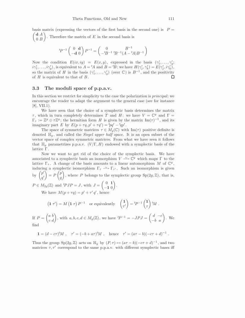
The addition formula has the following geometric interpretation:
Corollary 3.13. Let Θ be a symmetric theta divisor on T . For a ∈ T , putκ(a) := t∗aΘ + t∗−aΘ ∈ |2Θ| . There is a commutative diagram:
|2Θ|∗
≀
T
ϕ2Θ
==zzzzzzzz
κ!!DD
DDDD
DD
|2Θ|
Proof . After a translation by a point of order 2 we can assume Θ = Θτ for somesymplectic basis of Γ. We identify both |2Θτ | and its dual to P2g−1 using thebasis (θ[ε])ε∈Zg/2Zg . Then, by the addition formula,
κ(a) =(
θ[ε](a))
ε∈Zg/2Zg = ϕ2Θ(a) .
(For a more intrinsic description of the isomorphism |2Θ| ∼−→ |2Θ|∗ , see [21],p. 555.)
4 Curves and their Jacobians
In this section we denote by C a smooth projective curve (= compact Riemannsurface) of genus g .
4.1 Hodge theory for curves
We first recall briefly Hodge theory for curves, which is much easier than in thegeneral case. We start from the exact sequence of sheaves
0 → CC −→ OCd
−→ KC → 0 ,
118 Arnaud Beauville
where CC is the sheaf of locally constant complex functions, and KC (also denotedΩ1
C or ωC ) is the sheaf of holomorphic 1-forms. Taking into account H0(C, OC) =C and H1(C, KC) ∼= C (Serre duality), we obtain an exact sequence
0 → H0(C, KC)∂
−→ H1(C,C)p
−→ H1(C, OC) → 0 .
By definition g = dimH0(C, KC); by Serre duality we have also dimH1(C, OC) =g , hence dimH1(C,C) = 2g .
We put H1,0 := Im ∂ and H0,1 := H1,0 ; H1,0 is the subspace of classes inH1(C,C) which can be represented by holomorphic forms, and H0,1 by antiholo-morphic forms.
Lemma 4.1. Let α 6= 0 in H0(C, KC) ; then i∫
C α ∧ α > 0 .
Proof . Let z = x + iy be a local coordinate in an open subset U of C . We canwrite α = f(z)dz in U , so that
i
∫
U
α ∧ α =
∫
U
|f(z)|2 i dz ∧ dz =
∫
U
|f(z)|2 2 dx ∧ dy > 0 .
Proposition 4.2. H1(C,C) = H1,0 ⊕ H0,1 ; the map p induces an isomorphismH0,1 → H1(C, OC) .
Proof . The second assertion follows from the first and from the above exactsequence. For dimension reasons it suffices to prove that H1,0 ∩ H0,1 = (0). Letx ∈ H1,0 ∩ H0,1 . There exists α, β ∈ H0(C, KC) such that x = [α] = [β] , henceα − β = df for some C∞ function f on C . Then β ∧ β = df ∧ β = d(fβ),hence
∫
Cβ ∧ β = 0 by Stokes theorem. By the Lemma this implies β = 0 hence
x = 0.
Proposition 4.3. p(H1(C,Z)) is a lattice in H0,1 ; the hermitian form H onH0,1 defined by H(α, β) := 2i
∫
Cα ∧ β induces a principal polarization on the
complex torus H0,1/p(H1(C,Z)) .
Proof . The first assertion has already been proved (Section 2.1). Lemma 4.1shows that the form H is positive definite on H0,1 = H1,0 . Let a, b ∈ H1(C,Z);we have
a = α + α , b = β + β with α = p(a) , β = p(b) .
Their cup-product in H2(C,Z) = Z is given by
a · b =
∫
C
(α + α) ∧ (β + β) =1
2i
(
H(α, β) − H(β, α))
= Im(H)(α, β) ;
thus Im(H) induces on H1(C,Z) the cup-product, which is unimodular by Poincareduality.
The g -dimensional abelian variety JC := H0,1/p(H1(C,Z)) with the prin-cipal polarization H is called the Jacobian of C ; it plays an essential role in thestudy of the curve.
Theta Functions, Old and New 119
4.2 Line bundles on C
To study line bundles on C we use again the exact sequence (2.1):
0 → H1(C,Z)i
−→ H1(C, OC) −→ Pic(C)c1−→ H2(C,Z) ∼= Z→ 0 .
Here for a line bundle L on C , c1(L) is simply the degree deg(L) (through thecanonical isomorphism H2(C,Z) ∼= Z): deg(L) = deg(D) for any divisor D suchthat OC(D) ∼= L .
Note that i is the composition of the maps H1(C,Z) → H1(C,C)p
−→H1(C, OC) deduced from the inclusions of sheaves ZC ⊂ CC ⊂ OC . Hence:
Proposition 4.4. We have an exact sequence 0→JC−→Pic(C)deg−→Z→0 .
Thus JC is identified with Pico(C), the group of isomorphism classes ofdegree 0 line bundles on C – or the group of degree 0 divisors modulo linearequivalence. More precisely, one can show that JC is a moduli space for degree 0line bundles on C . This means the following. Let S be a complex manifold (oranalytic space), and let L be a line bundle on C×S . For s ∈ S , put Ls := LC×s .We say that (Ls)s∈S is a holomorphic family of line bundles on C parametrizedby S . If the line bundles Ls have degree 0, we get a map S → JC ; we want thismap to be holomorphic.
In fact we have even more: the line bundles L in JC form a holomorphicfamily. Namely, there exists a line bundle P on C × JC such that PL = L foreach L ∈ JC . Such a line bundle is called a Poincare line bundle. It is unique upto tensor product by the pullback of a line bundle on JC .
4.3 The Abel-Jacobi maps
As an illustration, choose a divisor D1 of degree 1 on C and define α : C → JCby α(p) = OC(p−D1). It is holomorphic (hence algebraic, since both C and JCare projective manifolds): indeed it is defined by the line bundle OC×C(∆−p∗D1)on C × C , where ∆ is the diagonal and p the first projection.
More generally, let C(d) denote the d-th symmetric power of the curve C ,that is, the quotient of Cd by the symmetric group Sd . This is a smooth variety:indeed since this a local question it suffices to prove it for the affine line C ; butthe map (z1, . . . , zd) 7→ (s1, . . . , sd), where si is the i -th elementary symmetricfunction of z1, . . . , zd , identifies C(d) to Cd . Using the map (p1, . . . , pd) 7→ p1 +· · · + pd we will view the elements of C(d) as effective divisors of degree d on C .
Now we choose a divisor Dd of degree d and define a map αd : C(d) →JC by αd(E) = OC(E − Dd). Again this is holomorphic, for instance becauseαd(p1 + · · ·+ pd) = α(p1) + · · ·+ α(pd) up to a constant. For E ∈ C(d) , the fiberα−1
d (αd(E)) is the linear system |E| (Sect. 3.6).
Proposition 4.5. For d ≤ g the map αd is generically injective.
Proof . By the observation preceding the Proposition we must prove2 h0(E) = 1for a general E ∈ C(d) . If D is an effective divisor, we have h0(D−p) = h0(D)−1
2We use the standard notations h0(F) := dimH0(C, F) for a sheaf F on C , and h0(D) :=h0(OC(D)) for a divisor D .
120 Arnaud Beauville
for p general in C , hence by induction h0(D − E) = h0(D) − d for E general inC(d) with d ≤ h0(D). Taking D = K gives h0(K − E) = g − d for d ≤ g , henceh0(E) = 1 by Riemann-Roch.
Corollary 4.6. αg : C(g) → JC is birational.
Another consequence is that the image of αg−1 : C(g−1) → JC is a divisorin JC . In fact:
Theorem 4.7 (Riemann). The image of αg−1 : C(g−1) → JC is a theta divisorof JC .
We have to refer to [1], p. 23 for the proof.
Remark 4.8. 1) Recall that the map αg−1 depends on the choice of a divisor D ,or equivalently of the line bundle L = OC(D), of degree g − 1. We will denote byΘL the corresponding theta divisor; explicitly:
ΘL = M ∈ JC | H0(M ⊗ L) 6= 0 .
2) There is a way to avoid the inelegant choice of a divisor Dd in the definitionof αd . Let Jd denote the set of isomorphism classes of line bundles of degree don C . Choosing a line bundle Ld of degree d defines a bijection JC → Jd (byM 7→ M ⊗ Ld ). This provides a structure of projective variety on Jd which doesnot depend on the choice of Ld . By construction Jd is isomorphic to JC , butthere is no canonical isomorphism.
Now we have a canonical map αd : C(d) → Jd defined simply by αd(E) =OC(E). In particular we have a canonical divisor Θ ⊂ Jg−1 , which is the locus ofthe line bundles L in Jg−1 with H0(L) 6= 0.
3) A consequence of the Riemann theorem is that the theta divisor is irre-ducible, so a Jacobian cannot be a product of non-trivial p.p.a.v. (Remark 3.10).
5 Vector bundles on curves
As explained in the introduction, generalized theta functions appear when wereplace JC , the moduli space of degree 0 line bundles on C , by the analogousmoduli spaces for higher rank vector bundles. We will now explain what thismeans.
5.1 Elementary properties
Let E be a vector bundle on C , of rank r . The maximum wedge power ∧rE isa line bundle on C , denoted det(E). Its degree is denoted by deg(E). It has thefollowing properties:
• In an exact sequence 0 → F → E → G → 0 we have det(E) ∼= det(F ) ⊗det(G);
Theta Functions, Old and New 121
• For any line bundle L on C , we have det(E ⊗ L) = det(E) ⊗ L⊗r .• (Riemann-Roch) h0(E) − h1(E) = deg(E) + r(1 − g).
It will be convenient to introduce the slope µ(E) :=deg(E)
r∈ Q . Thus
Riemann-Roch can be written h0(E) − h1(E) = r(µ(E) + 1 − g).
5.2 Moduli spaces
We have seen that the Jacobian of C parametrizes line bundles of degree 0, in thesense that for any holomorphic family (Ls)s∈S the corresponding map S → JCis holomorphic. Unfortunately such a nice moduli space does not exist in higherrank. Indeed we will show the following:
Lemma 5.1. Let L be a non-trivial line bundle on C with no base point (Sect.3.6) . There exists a holomorphic family of vector bundles (Et)t∈C on C such that:
Et∼= OC ⊕ OC for t 6= 0 E0
∼= L ⊕ L−1 .
Proof . We first take C = P1 and L = OP1(2). Put F := P1 × C , OF (k) :=pr∗1OP1(k). Consider the homomorphism
u : O⊕3F −→ OF (2) given by (X2, Y 2, tXY ) ,
where t is the coordinate on C and (X, Y ) the homogeneous coordinates on P1 .The map u is surjective, so its kernel is a rank 2 bundle F on P1 × C . We claimthat
Ft∼= OP1(−1)⊕2 for t 6= 0 F0
∼= OP1 ⊕ OP1(−2) .
There is a variety of ways to prove this. Perhaps the easiest is to observe thatany vector bundle on P1 is a direct sum of line bundles. Since Ft is a sub-bundleof O
⊕3P1 with determinant OP1(−2), it is either OP1(−1)⊕2 or OP1 ⊕ OP1(−2); the
first case occurs if and only if h0(Ft) = 0, that is, if and only if t 6= 0. Then thevector bundle F(1) on F has the required properties.
Now we consider the general case. Let s be a nonzero section of L ; we canfind a section t of L which does no vanish at the zeroes of s . Then (s, t) definesa map u : C → P1 such that u∗OP1(1) = L . The vector bundle E := (u, Id)∗F(1)on C × C has the required properties.
This implies that there is no reasonable moduli space M containing bothO
⊕2C and L ⊕ L−1 : the family constructed in the lemma would give rise to a
holomorphic map C→ M mapping Cr0 to a point, and 0 to a different point.There are two ways to deal with this problem. The sophisticated one, which wewill not discuss here, replaces moduli spaces by a more elaborate notion calledmoduli stacks. The reader interested by this point of view may look at [12].
Instead we will follow the classical (by now) approach, which eliminates cer-tain vector bundles, for instance those of the form L ⊕ L−1 which appear in thelemma; this is done as follows:
122 Arnaud Beauville
Definition 5.2. A vector bundle E on C is stable if µ(F ) < µ(E) for everysub-bundle 0 ( F E . It is polystable if it is a direct sum of stable sub-bundlesof slope µ(E) .
Theorem 5.3. There exists a moduli space Ms(r, d) for stable vector bundles ofrank r and degree d . It is a smooth connected quasi-projective manifold; it ad-mits a projective compactification M(r, d) whose points correspond to isomorphismclasses of polystable bundles.
Note that we do not claim that M(r, d) is a moduli space for polystablebundles; the situation is more complicated. We refer to [19] for a precise statementas well as the proof.
An important by-product of the proof is the fact that stability is an opencondition: if S is a variety and E a vector bundle on C ×S , the set of s ∈ S suchthat Es is stable is Zariski open in S ([19], Prop. 7.2.6).
5.3 The moduli space M(r)
We will in fact focus on a slightly different moduli space. The map det : M(r, d) →Jd which associates to a vector bundle its determinant is holomorphic. Let L be aline bundle of degree d ; the fiber det−1(L) is denoted M(r, L). We denote by Jr
the subgroup (isomorphic to (Z/rZ)2g ) of line bundles α ∈ JC with α⊗r ∼= OC .
Proposition 5.4. The map M(r, L) × JC → M(r, d) given by (E, λ) 7→ E ⊗ λidentifies M(r, d) with the quotient of M(r, L) × JC by Jr acting by α · (E, λ) =(E ⊗ α, λ ⊗ α−1) .
Proof . Let E in M(r, d). The pairs (F, λ) with F ∈ M(r, L), λ ∈ JC andE ∼= F ⊗ λ are obtained by taking λ ∈ JC with λ⊗r = det(E) ⊗ L−1 andF = E ⊗ λ−1 . We can always find such a λ , hence a pair (F, λ), and two suchpairs differ by the action of Jr .
Thus M(r, d) is determined by JC and M(r, L); from now on we will focuson the latter space. Note that for N ∈ Pic(C) the map E 7→ E ⊗ N inducesan isomorphism M(r, L) ∼−→ M(r, L ⊗ N⊗r); thus up to isomorphism, M(r, L)depends only of the degree d of L (mod. r ). When r and d are coprime M(r, L) =Ms(r, L) is smooth, and is a nice moduli space; however the most interesting casefor us will be d = 0, and the moduli space M(r, OC), which we will denote simplyM(r). This is also the moduli space of principal SL(r)-bundles, so its study fitsinto the more general theory of principal G-bundles for a semisimple group G .
Let us summarize in the next Proposition some elementary properties ofM(r), which follow from its construction (see [19]). From now on we will assumethat the genus g of C is ≥ 2 (for g ≤ 1 there are no stable bundles of degree 0and rank > 1).
Proposition 5.5. M(r) is a projective normal irreducible variety, of dimension(r2 − 1)(g − 1) , with mild singularities (so-called rational singularities) . Exceptwhen r = g = 2 , its singular locus is the locus of non-stable bundles.
Theta Functions, Old and New 123
As algebraic varieties, the moduli spaces M(r, L) are very different fromcomplex tori:
Proposition 5.6. The moduli space M(r, L) is unirational; that is, there existsa rational dominant map3 PN
99K M(r, L) .
Proof . Using the isomorphism M(r, L) ∼−→ M(r, L⊗N⊗r) we may assume deg(L) >r(2g − 1), so µ(E) > 2g − 1 for E ∈ M(r, L). Since E is polystable this impliesH0(E∗ ⊗ KC(p)) = 0 for any p ∈ C , hence by Serre duality H1(E(−p)) = 0.Then the exact sequence
0 → E(−p) → E → Ep → 0
gives for each p a surjection evp : H0(E) ։ Ep ; that is, the global sections of Egenerate E at p .
Now we claim that a general subspace of dimension r + 1 of H0(E) stillgenerates E at each point. For p ∈ C , let Zp be the subvariety of the Grassman-nian G(r + 1, H0(E)) consisting of subspaces V which do not span Ep . This isequivalent to dimV ∩ Ker(evp) ≥ 2, so Zp has codimension 2 (exercise!). ThusZ = ∪p∈CZp has codimension 1 in the Grassmannian; any V in the complementof Z generates E at each point. For such a V the evaluation map V ⊗ OC → Eis surjective. Its kernel is a line bundle; taking determinants we see that it is L−1 .Thus E∗ is the kernel of a surjective map V ∗ ⊗ OC → L .
Conversely, let G0 be the open subset of the Grassmannian G(r + 1, H0(L))parametrizing subspaces which span L at each point. For W ∈ G0 , we have anexact sequence
0 → FW −→ W ⊗C OCev−→ L → 0 ;
The dual EW := F ∗W is a rank r vector bundle with determinant L ; we obtain
in this way an algebraic family of such bundles, parametrized by G0 , such thatevery element of Ms(r, L) appears in the family. The subspaces W ∈ G0 suchthat EW is stable form a Zariski open subset G1 ⊂ G0 (Sect. 5.2), and we have asurjective map f : G1 → Ms(r, L) such that f(W ) = EW . Since Grassmanniansare rational varieties, composing f with a birational map PN
99K G1 gives therequired rational dominant map.
Corollary 5.7. Any rational map from M(r, L) to a complex torus is constant.
Proof . Let T = V/Γ be a complex torus. In view of the proposition, it sufficesto show that any rational map ϕ : PN
99K T is constant. Let p, q be two generalpoints of PN . The restriction of ϕ to the line 〈p, q〉 defines a map P1 → T ,which factors through V since P1 is simply connected, hence is constant. Thusϕ(p) = ϕ(q).
3In the rest of this section we assume some familiarity with the notion of rational maps – seee.g. [13], p. 490.
124 Arnaud Beauville
5.4 Rationality
The Luroth problem asks whether an unirational variety X is necessarily rational.The answer is positive when X is a curve (Luroth, 1876) or a surface (Castelnuovo,1895), but not in higher dimension (see for instance [9]).
While M(r, L) is known to be rational when deg(L) is prime to r [17], therationality of M(r) is an open problem, already for r = 2 and g = 3 – despitethe fact that in this case we have an explicit description of M(2) as a quartichypersurface in P7 (Sect. 6.5).
6 Generalized theta functions
6.1 The theta divisor
Since M(r) is simply connected, there is no hope to describe its line bundles bysystems of multipliers as for complex tori. However we may try to mimic thedefinition of the theta divisor: for L ∈ Jg−1 , we put
∆L := E ∈ M(r) | H0(E ⊗ L) 6= 0.
Theorem 6.1 ([10]). 1) ∆L is a Cartier divisor on M(r) .2) The line bundle L = O(∆L) is independent of L , and Pic(M(r)) = Z[L] .
Recall that an effective Cartier divisor is a subvariety locally defined by anequation – or, globally, as the zero locus of a section of a line bundle. On a singularvariety (as is M(r)) this is stronger than having codimension 1.
Proof . We will only show why ∆L is a divisor on the stable locus Ms(r), referring
to [10] for the rest of the proof. It is a consequence of the following lemma:
Lemma 6.2. Let S be a complex variety, (Es)s∈S a family of vector bundles onC , with µ(Es) = g − 1 for all s ∈ S . Then the locus
s ∈ S | H0(C, Es) 6= 0
is defined locally by one equation (possibly trivial).
Proof . We will use a general fact about cohomology of coherent sheaves (see [20],§5) : locally on S there exist vector bundles F, G and a homomorphism u : F → Gsuch that we have for each s in S an exact sequence
By Riemann-Roch we have h0(Es) = h1(Es), hence F and G have the same rank.We see that H0(C, Es) 6= 0 if and only if det(u(s)) = 0, that is, the section det(u)of det(G) ⊗ det(F )−1 vanishes at s , hence the lemma.
Coming back to M(r), the construction of the moduli space implies thatlocally for the complex topology, there is a “Poincare bundle”, that is a rank r
Theta Functions, Old and New 125
vector bundle E on C × V such that E|C×E∼= E for E in V . Applying the
lemma to E ⊗ L shows that ∆L is a divisor on Ms(r), unless ∆L = M(r). Butthis cannot hold: if α is a general element of JC , we have H0(L⊗α) = 0, henceα⊕r /∈ ∆L .
6.2 Generalized theta functions
By analogy with the case of Jacobians, the sections of H0(M(r), L⊗k) are calledgeneralized (or non-abelian) theta functions of order k . They are associated to thegroup SL(r) (there are more general theta functions associated to each complexreductive group, but we will not discuss them in these notes).
Like for complex tori, the first question we can ask about these theta functionsis the dimension of the space H0(M(r), L⊗k). The answer, much more intricatethan Theorem 3.5 for complex tori, is known as the Verlinde formula; it has beenfirst found by E. Verlinde using physics arguments, then proved mathematicallyin many different ways – see e.g. [29]. The formula is as follows:
dimH0(M(r), L⊗k) =( r
r + k
)g ∑
S∐T=[1,r+k]|S|=r
∏
s∈S
t∈T
∣
∣2 sinπs − t
r + k
∣
∣
g−1(6.1)
For r = 2 it reduces (after some trigonometric manipulations) to:
dimH0(M(2), L⊗k) = (k
2+ 1)g−1
k+1∑
i=1
1
(sin iπk+2 )2g−2
·
Even in rank 2, it is not at all obvious that the right hand side is an integer!
6.3 Linear systems and rational maps in Pn
This section is the logical continuation of Section 3.6; we again assume somefamiliarity with the notion of rational map ([13], p. 490). We keep our projectivevariety M and a line bundle L on M ; we do not assume B(L) = ∅ . We stillhave a map M rB(L) → |L|∗ , which we see as a rational map ϕL : M 99K |L|∗ .
Conversely, suppose given a rational map ϕ of M to a projective spaceP(V ). We assume that M is normal ; then the indeterminacy locus B of ϕhas codimension ≥ 2. We assume moreover that the line bundle ϕ∗OP(V )(1) onM r B extends to a line bundle L on M . By Hartogs theorem the restrictionmap H0(M, L) → H0(M rB, L) is bijective, so we get a pullback homomorphismϕ∗ : V ∗ → H0(M, L). We have a commutative diagram
|L|∗
P(tϕ∗)
M
ϕL
<<zz
zz
ϕ""E
EE
E
P(V )
126 Arnaud Beauville
Indeed for m general in M , ϕL(m) is the hyperplane of |L| formed by the divisorspassing through m ; its image under P(tϕ∗) is the hyperplane of P(V )∗ formed bythe hyperplanes of P(V ) passing through ϕ(m), and this corresponds by dualityto the point ϕ(m) ∈ P(V ).
6.4 The theta map
We go back to our moduli space M(r) and the generator L of its Picard group.The next step is to ask for the map defined by the linear systems |L⊗k| . In factwe will concentrate on the simplest one, namely ϕL . Our task will be to give ageometric description of this map. In order to do this we associate to each vectorbundle E ∈ M(r) the locus
θ(E) := L ∈ Jg−1 | H0(E ⊗ L) 6= 0
Proposition 6.3. θ(E) is either equal to Jg−1 , or is a divisor in Jg−1 , belongingto the linear system |rΘ| .
Proof . Consider the vector bundle E ⊗ P on C × Jg−1 , where P is a Poincareline bundle (Section 4.2). It defines the family of vector bundles (E ⊗ L)L∈Jg−1
on C . These bundles have slope g − 1, hence we can apply Lemma 6.2, whichshows that θ(E) is defined locally by one (possibly trivial) equation.
Let S be an irreducible variety, and E a vector bundle on C × S , withdeg(Es) = 0 for each s . Lemma 6.2, applied to the vector bundle E ⊗ P onC ×S × Jg−1 , gives a line bundle N on Jg−1 ×S and a section τ of N with zerolocus Z = ∪s θ(Es). Put
So := s ∈ S | θ(Es) 6= Jg−1 ;
So is the projection on S of the complement of Z in Jg−1 × S , so it is a Zariskiopen subset of S .
Applying this locally to our moduli space M(r), we see that the vector bun-dles E ∈ M(r) with θ(E) = Jg−1 form a closed analytic (and therefore alge-braic) subset of M(r). Let M(r)o be the complement of this subset. WhenE runs through M(r)o , the Chern class c1(θ(E)) is constant. So if we fixE0 ∈ M(r)o , we have a rational map M(r) 99K Pico(Jg−1) mapping E ∈ M(r)o
to OJ(θ(E) − θ(E0)). By Corollary 5.7 this map is constant, hence OJ(θ(E)) isindependent of E .
Let α1, . . . , αr be distinct elements of JC . We have
θ(α1 ⊕ · · · ⊕ αr) = t∗α1Θ + · · · + t∗αr
Θ ∈ |rΘ|
(see Corollary 2.11). Thus whenever θ(E) 6= Jg−1 we have θ(E) ∈ |rΘ| .
Thus we have a rational map θ : M(r) 99K |rΘ| .
Theorem 6.4 ([6]). There is a natural isomorphism
H0(M(r), L) ∼−→ H0(Jg−1, O(rΘ))∗
Theta Functions, Old and New 127
making the following diagram commutative:
|L|∗
≀
M(r)
ϕL
<<xx
xx
θ""F
FF
F
|rΘ|
Sketch of proof : For L ∈ Jg−1 , let HL be the hyperplane in |rΘ| consisting ofthe divisors passing through L . By definition the pullback of HL under θ is thedivisor ∆L . Thus, as explained in Section 6.3, we get a commutative diagram
|L|∗
λ
M(r)
ϕL
<<xx
xx
θ""F
FF
F
|rΘ|
with λ := P(tθ∗). It remains to prove that λ is bijective. Surjectivity is notdifficult, let us prove it in the case r = 2. If λ is not surjective, the image of θ iscontained in a hyperplane of |2Θ| . But this image contains all the divisors θ(α ⊕α−1) = t∗αΘ + t∗−αΘ for α ∈ JC ; and Corollary 3.13 implies that these divisorsspan |2Θ| (otherwise the image of ϕ2Θ would be contained in a hyperplane).
We have dim |rΘ| = rg − 1 by Theorem 3.5, so the crucial point is to provethe same equality for dim |L| . Of course this follows (in a non-trivial way) fromthe Verlinde formula (6.1); in [6], since the Verlinde formula was not yet available,we constructed a rational dominant map from a certain abelian variety to themoduli space, and applied Theorem 3.5 to get the result.
Corollary 6.5. The base locus of the linear system |L| on M(r) is the set ofvector bundles E ∈ M(r) such that θ(E) = Jg−1 .
Thus the rather mysterious map ϕL is identified with the more concrete mapθ ; one usually refers to θ , or ϕL , as the theta map. We will now see that thisexplicit description allows a good understanding of the theta map in the rank 2case.
6.5 Rank 2
In rank 2 the theta map is by now fairly well understood. We summarize what isknown in one theorem:
128 Arnaud Beauville
Theorem 6.6. 1) The theta map θ : M(2) → |2Θ| is a morphism.2) If C is not hyperelliptic or g = 2 , θ is an embedding.3) If C is hyperelliptic of genus ≥ 3 , θ is 2-to-1 onto its image in |2Θ| ,
and this image admits an explicit description.
This is the conjunction of various results. Part 1) is due to Raynaud [28],part 3) to Bhosle-Ramanan [11]. In case 2), the fact that θ is generically injectivewas proved in [2]; from this Brivio and Verra deduced that θ embeds Ms(2), andthis was extended to M(2) in [14].
Recall that M(2) has dimension 3g − 3. In particular:
Corollary 6.7 ([23]). For g = 2 , θ : M(2) → |2Θ| ∼= P3 is an isomorphism.
Consider the map k : JC → M(2) given by k(L) = L⊕L−1 . The compositionθ k is the map κ studied in Section 3.8; thus k embeds the Kummer variety K ofJC into M(2), and the restriction of θ to K is the natural embedding of K into|2Θ| . For g > 2 K is the singular locus of M(2) (Proposition 5.5); when C isnot hyperelliptic, we obtain a variety in |2Θ| which is singular along the Kummervariety.
For g = 3 and C not hyperelliptic, a very nice application appears in [24].In that case dimM(2) = 6, so θ embeds M(2) as a hypersurface in |2Θ| ∼= P7 .It is not difficult to prove that it has degree 4 (for instance by computing itscanonical bundle). Now Coble had found long ago that there is a unique quartichypersurface in |2Θ| which is singular along the Kummer variety, for which hehad written down an explicit equation (see [3] for a modern account). Thereforethis hypersurface is M(2).
We will illustrate the methods used to prove the above results by giving theproof of 1).
6.6 Raynaud’s theorem
We will prove part 1) of Theorem 6.6 in the following form:
Proposition 6.8. Let E ∈ M(2) . Then θ(E) 6= Jg−1 .
Proof . If E = L ⊕ L−1 , we have θ(E) = ΘL + ΘL−1 6= Jg−1 . Therefore we mayassume that E is stable.
Suppose θ(E) = Jg−1 . Put F = E ⊗L for some L in Jg−1 ; our hypothesisbecomes h0(F ⊗α) > 0 for all α ∈ JC . Put h := minα∈JC h0(F ⊗α). ReplacingF by F ⊗ α for an appropriate α we may assume h0(F ) = h . We will use thesemi-continuity theorem in cohomology, which implies that there is a Zariski opensubset U ⊂ JC (containing 0) such that h0(F ⊗ α) = h for α ∈ U ([20], §5).
Put F ′ := F ∗ ⊗ KC ; let p ∈ C . The Riemann-Roch theorem gives(
h0(F (p)) − h0(F ))
+(
h0(F ′) − h0(F ′(−p))
= 2 .
For p general we have h0(F ′) − h0(F ′(−p) ≥ 1, hence h0(F (p)) − h0(F ) ≤ 1.But h0(F (p)) = h would imply h0(F (p− q)) < h for q general, contradicting thedefinition of h . Thus h0(F (p)) = h + 1.
Theta Functions, Old and New 129
Put G := F (p). We have h0(G) = h+1, and h0(G(−q)) = h0(F (p− q)) = hfor q general in C . From the exact sequence
0 → G(−q) → G → Gq → 0
we see that the global sections of G generate a rank 1 subsheaf L0 of G . Thisis not necessarily a sub-line bundle because the quotient G/L0 may have torsion;but it is contained in a unique sub-line bundle L , the kernel of the projection fromG to the torsion-free quotient of G/L (sometimes called the saturation of L0 inG). This sub-line bundle L has the property that any rank 1 subsheaf M ⊂ Gwith h0(M) > 0 is contained in L . Indeed if s is a nonzero section of M , at ageneral point x of C s(x) generates Mx and Lx ; therefore the map M → G/Lis zero generically, hence everywhere.
Now take q, r general in C and consider G(q−r). As before its global sectionsgenerate a sub-line bundle L′ ⊂ G(q − r). But we have L(q − r) ⊂ G(q − r),and h0(L(q − r)) > 0 since h0(L) = h0(G) ≥ 2. Hence L(q − r) ⊂ L′ . Butsymmetrically we have L′(r − q) ⊂ L , hence L(q − r) = L′ . In particular we findh0(L(q−r)) = h = h0(L) for q, r general in C . This implies h0(L(q)) = h0(L)+1,hence by Riemann-Roch h0(K ⊗ L−1) = h0(K ⊗ L−1(−q)) for q general; this ispossible only if h0(K ⊗ L−1) = 0. Applying again Riemann-Roch and usingh0(L) ≥ 2, we get deg(L) ≥ g + 1 > µ(G), a contradiction.
6.7 Higher rank
In contrast with the rank 2 case, not much is known in higher rank. It is knownsince [28] that there exist stable bundles E with θ(E) = Jg−1 – that is, basepoints for the linear system |L| ; in fact, they exist as soon as r ≥ g + 2, and evenr ≥ 4 if C is hyperelliptic [26]. On the other hand, in rank 3 there are no basepoints for g = 2 [28], g = 3 [4], or if C is general enough [28].
The situation is somewhat particular when g = 2, since dimM(r) = dim |rΘ| =r2 − 1.
Proposition 6.9. Let g = 2 .
1) θ : M(r) 99K |rΘ| is generically finite.2) Its degree is 1 for r = 2 , 2 for r = 3 , 30 for r = 4 .
Part 1) is proved in [4]. The rank 2 case has been discussed in Corollary6.7. In rank three θ : M(3) → |3Θ| ∼= P8 is a double covering, branched along asextic hypersurface which can be explicitly described [25]. The case r = 4 is dueto Pauly [27].
Let us conclude with a
Conjecture 6.10. For g ≥ 3 , the theta map θ : M(r) 99K |rΘ| is generically2-to-1 onto its image if C is hyperelliptic, and generically injective otherwise.
This is unknown even for r = g = 3.
130 Arnaud Beauville
6.8 Further reading
There are a number of topics which I would have liked to cover in these lecturesbut could not by lack of time. Here are a few of them, with references to theliterature:
• The beautiful interplay between curves and their Jacobians: Torelli theorem,Schottky problem, etc. A nice overview can be found in [22]; some of thetopics are developed in [1].
• The heat equation and its extension to generalized theta functions. Theoriginal paper [16] of Hitchin is of course somewhat advanced, but still quitereadable.
• Higgs bundles. Though not directly related to generalized theta functions,this is an important subject with many applications. Here again one can lookat the original paper [15] of Hitchin; see also [7] for a short introduction.
• Principal bundles. This amounts to replace the group SL(r) by any semi-simple group. Essentially all we have said extends to this set-up. Thereare few results on the theta map, see [5] for the orthogonal and symplecticgroups.
References
[1] E. Arbarello, M. Cornalba, P. Griffiths, J. Harris: Geometry of algebraic
curves. Vol. I. Grund. Math. Wiss. 267. Springer-Verlag, New York, 1985.[2] A. Beauville: Fibres de rang 2 sur les courbes, fibre determinant et fonctions
theta. Bull. Soc. Math. France 116 (1988), 431–448.[3] A. Beauville: The Coble hypersurfaces. C. R. Math. Acad. Sci. Paris 337
(2003), no. 3, 189–194.[4] A. Beauville: Vector bundles and theta functions on curves of genus 2 and
3. Amer. J. of Math. 128 (2006), 607–618.[5] A. Beauville: Orthogonal bundles on curves and theta functions. Ann. Inst.
Fourier 56 (2006), 1405–1418.[6] A. Beauville, M.S. Narasimhan, S. Ramanan: Spectral curves and the gen-
eralised theta divisor. J. Reine Angew. Math. 398 (1989), 169–179.[7] S. Bradlow, O. Garcıa-Prada, and P. Gothen: What is ... a Higgs bundle?
Notices of the AMS 54, no. 8 (2007).[8] O. Debarre: Complex Tori and Abelian Varieties. SMF/AMS Texts and
Monographs 11. AMS, Providence, 2005.[9] P. Deligne: Varietes unirationnelles non rationnelles. Seminaire Bourbaki
(1971/1972), Exp. No. 402, pp. 45-57. Lecture Notes in Math. 317, Springer,Berlin, 1973.
[10] J.M. Drezet, M.S. Narasimhan: Groupe de Picard des varietes de modules
de fibres semi-stables sur les courbes algebriques. Invent. math. 97 (1989),53–94.
[11] U. Desale, S. Ramanan: Classification of vector bundles of rank 2 on hyper-
[12] T. Gomez: Algebraic stacks. Proc. Indian Acad. Sci. Math. Sci. 111 (2001),no. 1, 1–31.
[13] P. Griffiths, J. Harris: Principles of Algebraic Geometry. Wiley-Interscience,New York, 1978.
[14] B. Van Geemen, E. Izadi: The tangent space to the moduli space of vector
bundles on a curve and the singular locus of the theta divisor of the Jacobian.J. Algebraic Geom. 10 (2001), 133–177.
[15] N. Hitchin: The self-duality equations on a Riemann surface. Proc. LondonMath. Soc. (3) 55 (1987) 59–126.
[16] N. Hitchin: Flat connections and geometric quantization. Comm. Math.Phys. 131 (1990), 347–380.
[17] A. King, A. Schofield: Rationality of moduli of vector bundles on curves.Indag. Math. (N.S.) 10 (1999), no. 4, 519–535.
[18] H. Lange, M.S. Narasimhan: Squares of ample line bundles on abelian vari-
eties. Exposition. Math. 7 (1989), no. 3, 275–287.[19] J. Le Potier: Lectures on vector bundles. Cambridge Studies in Advanced
Mathematics, 54. Cambridge University Press, Cambridge, 1997.[20] D. Mumford: Abelian Varieties. Oxford University Press, London, 1970.[21] D. Mumford: Prym Varieties I. Contributions to analysis, 325–350. Aca-
demic Press, New York, 1974.[22] D. Mumford: Curves and Their Jacobians. Appendix to The Red Book of
Varieties and Schemes, LN 1358, Springer-Verlag, Berlin, 1999.[23] M.S. Narasimhan, S. Ramanan: Moduli of vector bundles on a compact
Riemann surface. Ann. of Math. 89 (1969), 19–51.[24] M.S. Narasimhan, S. Ramanan: 2θ -linear systems on Abelian varieties. Vec-
tor bundles on algebraic varieties, 415–427; Oxford University Press, London,1987.
[25] A. Ortega: On the moduli space of rank 3 vector bundles on a genus 2 curve
and the Coble cubic. J. Algebraic Geom. 14 (2005), no. 2, 327–356.[26] C. Pauly: On the base locus of the linear system of generalized theta func-
tions. Math. Res. Lett. 15 (2008), no. 4, 699–703.[27] C. Pauly: Rank four vector bundles without theta divisor over a curve of
genus two. Adv. Geom. 10 (2010), no. 4, 647–657.[28] M. Raynaud: Sections des fibres vectoriels sur une courbe. Bull. Soc. math.
France 110 (1982), 103–125.[29] C. Sorger: La formule de Verlinde. Seminaire Bourbaki, Exp. 794, 1994/95.


![THETA FUNCTIONS ON VARIETIES WITH EFFECTIVE ...THETA FUNCTIONS 3 degeneration. This point of view incorporates, for example, all Batyrev-Borisov mirrors [Gr1]. However, it is not clear](https://static.documents.pub/doc/80x56/6067e60b962dd12eb4717a4a/theta-functions-on-varieties-with-effective-theta-functions-3-degeneration.jpg)

![Computing Riemann Theta Functions - University of Washington · Riemann theta functions in their full generality, as de ned in (1), were considered rst by Wirtinger [21], whose convention](https://static.documents.pub/doc/80x56/5fbfd8ddb8304b37c23f5986/computing-riemann-theta-functions-university-of-washington-riemann-theta-functions.jpg)


![Computing Riemann theta functions in Sage with …depts.washington.edu/.../pdfs/Swierczewski_Deconinck1.pdfRiemann theta functions can be associated with Riemann surfaces [15] and](https://static.documents.pub/doc/80x56/5f0ccc2f7e708231d4372e2c/computing-riemann-theta-functions-in-sage-with-depts-riemann-theta-functions-can.jpg)


