TheThree-DimensionalNormal-Distributions Transform — an ...

Doctoral Dissertation

The Three-Dimensional Normal-Distributions Transform— an Efficient Representation for Registration,

Surface Analysis, and Loop Detection

Martin Magnusson

Technology

Örebro Studies in Technology 36

örebro 2013

The Three-Dimensional Normal-Distributions Transform

— an Efficient Representation for Registration,


Örebro Studies in Technology 36

Martin Magnusson

The Three-Dimensional Normal-Distributions Transform

— an Efficient Representation for Registration,


© Martin Magnusson, 2013

Title: The Three-Dimensional Normal-Distributions Transform— an Efficient Representation for Registration, Surface Analysis, and

Loop Detection

Publisher: Örebro University, 2013

www.publications.oru.se

Editor: Heinz [email protected]

Printer: intellecta infolog, Kållered 10/2009

ISSN 1650-8580

ISBN 978-91-7668-696-6

Abstract

This dissertation is concerned with three-dimensional (3D) sensing and 3D scanrepresentation. Three-dimensional records are important tools in several, quitediverse, disciplines; such as medical imaging, archaeology, and mobile robotics.In the case of mobile robotics (the discipline that is primarily targeted by thepresent work), 3D scanning of the environment is useful in several subtasks,such as mapping, localisation, and extraction of semantic information fromthe robot’s environment. This dissertation proposes the normal-distributionstransform, NDT, as a general 3D surface representation with applications inscan registration, localisation, loop detection, and surface-structure analysis.

Range scanners typically produce data in the form of point clouds. After ap-plying NDT to the original discrete point samples, the scanned surface is insteadrepresented by a piecewise smooth function with analytic first- and second-order derivatives. Such a representation has a number of attractive properties.

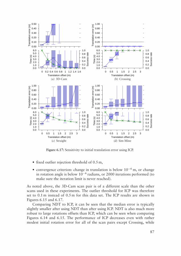
The smooth function representation makes it possible to use standard meth-ods from the numerical optimisation literature, such as Newton’s method, forscan registration. This dissertation extends the original two-dimensional (2D)NDT registration algorithm of Biber and Straßer to 3D and introduces a num-ber of improvements. By using a multiresolution discretisation technique andtrilinear interpolation, some of the discretisation issues present in the basic reg-istration algorithm can be overcome. With these extensions, the robustness ofthe registration algorithm is substantially increased. The 3D-NDT scan registra-tion algorithm is compared to current de facto standard registration algorithms.The algorithms are evaluated using exhaustive experiments with both simulatedand real-world scan data. 3D-NDT scan registration with the proposed exten-sions is shown to be faster and, in most cases, more accurate and more robustto poor initial pose estimates than the popular ICP scan registration algorithm.An additional benefit is that 3D-NDT registration provides a reliable confidencemeasure of the result with little additional effort.

Furthermore, a kernel-based extension to 3D-NDT for registering coloureddata is proposed. As opposed to the original algorithm, which uses one metricnormal distribution for each quantum of space, Colour-NDT uses three com-ponents, each associated with a colour. This representation allows colouredscans with little geometric features to be registered. When both 3D scan data

v

and visual-image data are available, it is also possible to do scan registrationusing local visual features of the image data. However, approaches based onlocal features typically use only a small fraction of the available 3D points forregistration. In contrast, Colour-NDT uses all of the available 3D data. Thisdissertation proposes to use a combination of local visual features and Colour-NDT for robust registration of coloured 3D point clouds in the presence ofstrong repetitive textures or dynamic changes between scans.

Also building on NDT, a new approach using 3D laser scans to performappearance-based loop detection for mobile robots is proposed. Loop detectionis an important problem in the SLAM (simultaneous localisation and mapping)domain. 2D laser-based approaches are bound to fail when there is no flat floor.Two of the problems with 3D approaches that are addressed in this dissertationare how to handle the greatly increased amount of data and how to efficientlyobtain invariance to 3D rotations. The proposed approach uses only the appear-ance of 3D point clouds to detect loops and requires no pose information. Itexploits the NDT surface representation to create feature histograms based onlocal surface orientation and smoothness. The surface-shape histograms com-press the input data by two to three orders of magnitude. Because of the highcompression rate, the histograms can be matched efficiently to compare the ap-pearance of two scans. Rotation invariance is achieved by aligning scans withrespect to dominant surface orientations. In order to automatically determinethe threshold that separates scans at loop closures from others, the proposedapproach uses expectation maximisation to fit a Gamma mixture model to theoutput similarity measures. Also included is a discussion of the problem of de-termining ground truth in the context of loop detection and the difficulties incomparing the results of the few available methods based on range information.

In order to enable more high-level tasks than scan registration, localisation,and mapping, it is desirable to also extract semantic information from 3D mod-els. The ability to automatically segment the map into meaningful componentsis necessary to further increase autonomy. Information that may be useful toextract in a mobile robot context includes walls, doors, and drivable surfaces.One important task where 3D surface analysis may be useful is boulder detec-tion for underground mining vehicles. This dissertation presents a method, alsoinspired by the NDT surface representation, that provides clues as to where thepile is, where the bucket should be placed for loading, and where there are ob-stacles. The points of 3D point clouds are classified based on the surroundingsurface roughness and orientation. Other potential applications of the proposedalgorithm include extraction of drivable paths over uneven surfaces.

In addition to the aforementioned contributions, the dissertation also in-cludes an overview of range sensors and their utility in mining applications.

Keywords: NDT, 3D sensing, surface representation, registration, loop detec-tion, surface analysis, mobile robotics, localisation, mapping.

vi

Sammanfattning på svenska

Tredimensionella (3D) modeller är viktiga verktyg inom många discipliner somsinsemellan är mycket olika. Ett exempel är medicinsk bildbehandling, där 3D-bilder används för att visa patienters organ utan att läkaren behöver operera.Ett annat exempel är arkeologi, där 3D-modeller av antika föremål kan sparasutan att skadas av en allt mer korrosiv miljö. Digitala 3D-modeller gör detockså möjligt att att analysera arkeologiska fynd på ett sätt som annars intevore praktiskt genomförbart. Ytterligare ett användningsområde är inom mobilrobotik, där 3D-modeller av omgivningen är användbara för flera deländamål,såsom kartläggning, lokalisering och utvinning av semantisk information frånrobotens omgivande miljö.

För att kunna använda de tredimensionella modellerna krävs en formellbeskrivning som kan användas för att matematiskt representera dem och lag-ra dem i en dator. Det centrala temat för den här avhandlingen är en sådanformell beskrivning, nämligen normalfördelningstransformen, eller NDT (”thenormal-distributions transform” på engelska). NDT tillhandahåller en fördel-aktig beskrivning av 3D-data. Normalt är sådana data tillgängliga i form avostrukturerade ”punktmoln”, det vill säga en samling mätpunkter, var och enmed en viss position. Punkterna, som har uppmätts från en yta, utgör en mo-dell av det objekt som avlästs. Efter det att NDT tillämpats på ett punktmolnbeskrivs i stället den avlästa ytan som en jämn och styckvis kontinuerlig funk-tion med analytiska derivator. Jämfört med punktmoln är en sådan beskrivningfördelaktig på flera sätt.

När man skapar en 3D-modell av ett fysiskt objekt är det ofta så att helaområdet man är intresserad av inte kan läsas av på en gång — antingen för attvissa delar är skymda, för att objektet är för stort eller för att objektet i sig ärfragmenterat. Därför måste man som regel använda sig av så kallad registrering— det vill säga sammanfogning av de olika delarna — för att skapa en komplettmodell. För att kunna passa ihop delarna av 3D-modellen måste man hitta denkorrekta positionen och orienteringen för alla delar, det vill säga deras poser.Att passa ihop en fragmenterad 3D-modell kan jämföras med att lägga pussel.Det gäller att hitta rätt ställe för att passa in varje bit. Att hitta rätt pose ären uppgift för registreringsalgoritmer. Parvis registrering är processen att hittaden pose där ett fragment bäst passar ihop med ett annat, under antagandet

vii

att de två delarna överlappar varandra till viss del. Utgående från en uppskatt-ning av posen för ett fragment i relation till ett överlappande fragment, får manmed hjälp av en lokal registreringsalgoritm fram en förbättrad uppskattningav posen. En bra registreringsalgoritm ska vara robust vad gäller stora fel iden ursprungliga uppskattningen av posen och snabbt producera en pose sommer exakt passar ihop de två delarna. Förutom för att skapa en sammanfogadmodell är registrering också användbart för pose-spårning för tillämpningar in-om mobil robotik, där en robot färdas genom ett område medan den läser avomgivningen och på så sätt skapar delmodeller av sin omgivning. Efter regi-strering vet man exakt vid vilken position och i vilken riktning varje delmodellgjorts, och därmed är det möjligt att återskapa robotens väg genom området.Genom att använda NDT är det möjligt att utföra registrering med hjälp avstandardmetoder från den digra litteratur som finns inom numerisk optimering,till exempel Newtons metod.

Den här avhandlingen fokuserar framför allt på 3D-avläsning för mobilarobotar, och i första hand riktar den in sig på tillämpningar för autonoma (detvill säga självgående) underjordiska gruvfordon. Gruvdrift har alltid varit, ochär fortfarande, mycket riskfyllt. Människor som arbetar under jord måste utståmånga faror. Följande citat från en kinesisk gruvarbetare speglar den farligaarbetsmiljön:

Om jag hade varit högsta chef i Kina skulle jag inte låta människorjobba i gruvor utan låta dem plantera träd i förorterna i stället. [84]

Många steg har tagits för att förbättra säkerheten, men ännu idag offras mångaliv i gruvolyckor. Bara i Kina dör tusentals människor varje år. Enligt officiellstatistik från Kinas statliga administration för arbetssäkerhet dog inte mindreän 8 726 människor i gruvolyckor år 2004 — det betyder i snitt 23 personerper dag! Olycksstatistiken är skrämmande, och 2004 var inte något ovanligtår. Siffrorna är visserligen betydligt lägre i resten av världen, men säkerhet förunderjordisk gruvpersonal är fortfarande en mycket viktig fråga. Autonomagruvfordon skulle vara till stor nytta för gruvindustrin, och mätningar i 3D ärett viktigt instrument för att kunna nå det målet. Med hjälp av registrering ärdet möjligt att konstruera tredimensionella kartor av gruvtunnlar med ett mini-mum av manuell inblandning. Sådana 3D-modeller kan användas av framtidaautonoma fordon för lokalisering och planering, och de är också användbaraför flera praktiska syften redan idag. Som exempel kan nämnas att säkerstäl-la att nya tunnlar verkligen har den form och sträckning de ska ha enligt deursprungliga planerna. På många platser finns krav på dokumentation av hurmycket material som har forslats bort i en gruva, och om det finns en detalje-rad 3D-modell av gruvan är det lätt att mäta den volymen. Registrering kanockså användas för noggrann positionering när man ska utföra semi-autonomborrning.

Att lokalisera sig i underjordiska gruvor är långt ifrån en enkel uppgift. Ettenkelt men otillräckligt sätt att uppskatta positionen är att använda så kallad

viii

död räkning och beräkna förflyttningen utifrån hjulens rotation. Noggrannhe-ten blir dock dålig, särskilt när hjulen slirar eller fordonet svänger, och fel ipositionen ackumuleras oacceptabelt snabbt. Död räkning kan förbättras medhjälp av tröghetsnavigering, där man använder en sensor som mäter förflytt-ning med accelerometrar och gyroskop. Men även då växer felet okontrolleratöver längre avstånd. Ett vanligt, och tillförlitligt, sätt att bestämma positioneni underjordiska miljöer är att utföra triangulering med en så kallad totalstation,monterad på stativ. Jämfört med de lasersensorer som är vanliga inom robobo-tikvärlden går det ohyggligt långsamt att mäta avstånd med totalstationer, ochdet krävs också manuellt arbete för att använda en totalstation. Ytterligare ettalternativ för att lokalisera sig är att skapa infrastruktur, till exempel magnetis-ka spår i golvet eller särskilda reflektorer med kända positioner. En autonommaskin ska dock inte behöva vara beroende av sådana modifikationer. När for-donet är ovan jord är det ibland möjligt att använda globala navigationssatellit-system, till exempel GPS. Under markytan är det naturligtvis inte möjligt attanvända navigationssatelliter. Även för tillämpningar ovan jord finns det pro-blem med sådana system. På många platser är det svårt att se tillräckligt mångasatelliter, och när mottagaren är nära större byggnader har satellitnavigeringofta dålig noggrannhet på grund av indirekta signalvägar — det vill säga, satel-litsignalerna studsar på väggarna. I stället för att förlita sig på någon av ovannämnda lokaliseringsmetoder kan ett fordon som är utrustat med en 3D-sensori stället använda registrering för att upprätthålla en tillförlitlig uppskattning avsin pose, på sätt som beskrivs i den här avhandlingen.

Även med noggranna registreringstekniker ackumuleras fel i robotens upp-fattning om sin pose över längre avstånd. När fordonet väl återvänder till entidigare besökt plats är det möjligt att korrigera poseinformationen. Det ac-kumulerade felet kan då också fördelas över hela robotens väg och på så sättkan kartan göras sammanhängande. Det största problemet är att på ett pålitligtsätt upptäcka att man har varit på en plats förut. När det ackumulerade feletär stort är det inte möjligt att använda robotens uppfattning om sin positionför att härleda att den återbesöker en viss plats. Det kan därför vara nödvän-digt att använda utseendet på avläsningar av omgivningen; med andra ord, attkänna igen en plats bara genom att jämföra dess utseende med tidigare avläs-ningar. Även om det är relativt lätt för en mänsklig observatör att känna igentvå 3D-modeller från samma plats så är det inte alls enkelt att göra det automa-tiskt med en dator. Problemet att inse att en plats har besökts förut genom attkänna igen en avbildning av den är ett exempel på det mer generella problemsom kallas data-association: att härleda vilka indata som svarar mot samma ex-terna förutsättningar. NDT tillhandahåller en kompakt men ändå särskiljandebeskrivning av 3D-modeller, som kan utnyttjas för att skapa en kraftigt kom-primerad utseendedeskriptor som utgör en formell beskrivning av en avläsningsutseende. Tack vare den höga kompressionsgraden är det möjligt att jämföra ettmycket stort antal avläsningar på kort tid. Den här avhandlingen presenteraren NDT-baserad metod som är tillräckligt särskiljande för att med mycket få

ix

falsklarm kunna detektera en stor del av de avläsningar som skapats på sammaplats.

För att kunna utföra uppgifter på en högre abstraktionsnivå än vad somkrävs för registrering, lokalisering och kartläggning är det önskvärt att kunnautläsa semantisk information från de tillgängliga 3D-modellerna. Att ha en san-ningsenlig 3D-karta är en sak, men att automatiskt kunna dela upp kartan imeningsfulla komponenter och att ”förstå” vad de representerar är nödvändigtför att ytterligare kunna utöka autonomiteten. När det gäller mobila robotarkan det bland annat vara användbart att kunna utskilja var väggar och dörrarfinns och vilka ytor som går att köra på. I en underjordisk gruvapplikationär blockdetektering en viktig uppgift där semantisk analys i 3D kan vara an-vändbar. De semi-autonoma gruvmaskiner som finns idag är kapabla att följatunnlar och dumpa sin last på särskilda platser. Autonom lastning av materialär å andra sidan till stor del fortfarande ett olöst problem. Givet en hög medmaterial som ska lastas i maskinens skopa är det i allmänhet inte att rekommen-dera att köra skopan in i högen i blindo. I gruvor finns det ofta hinder i högen iform av stora stenblock. För att fylla skopan är det nödvändigt att undvika förstora stenblock. Den här avhandlingen presenterar en metod, också den inspi-rerad av NDT, som kan ge ledtrådar om var högen är, var skopan bör placerasför lastning, och var det finns hinder.

x

Acknowledgements

I would like to begin by thanking Achim Lilienthal, who has been my super-visor for the larger part of my graduate studies, for his many insightful com-ments, friendly support, and persistent strong dedication to the task. I am alsovery thankful to Tom Duckett, my initial supervisor, for taking me in at AASS.Thanks for your support, supervision, and friendship.

I am deeply indebted to Peter Biber, with whom I shared the office duringthe fall of 2004, for his initial work on NDT, which is the foundation for thisthesis.

I also owe a great deal to Benjamin Huhle, with whom I collaborated on thework on Colour-NDT during the fall of 2007. Thanks for all your work and forvery valuable discussions on NDT. Thanks also for your company, both insideand out of the lab.

Naturally, I am also very thankful to Atlas Copco Rock Drills AB for em-ploying me during this time. Thank you, Johan Larsson, for your support andcompany, for driving to and from Västerås, and also for helping out with im-ages and data collection. Thanks to Rolf Elsrud, Kim Halonen, Michael Krasser,and Roland Pettersson for help with data collection, and to Richard Hendebergfor collecting video data from the Kvarntorp mine. Thanks to Ilka Ylitalo ofOutokumpu Oy for helping to evaluate the work on boulder detection.

Optab Optronikinnovation AB provided me with a very spacious officewhen I first started this work — thanks for that. I would especially like to thankHenrik Gustafsson for all the help setting up the Optab scanner prototype andLars-Erik Skagerlund for enthusiastic and helpful input.

I would also like to extend my gratitude to Joachim Hertzberg from theUniversity of Osnabrück for valuable comments on my licentiate thesis. Andmany thanks to Andreas Nüchter for providing ground-truth data and illus-trations for the work on loop detection, and for collaborating with me whencomparing ICP and NDT.

Thanks, also, to all the people at AASS. Thanks to Henrik Andreasson foryour ideas and comments, and all the work on Tjorven. Likewise, I am thankfulto Martin Persson and Christoffer Wahlgren for helping to maintain Tjorven,as well as Per Sporrong and Bo-Lennart Silfverdal for helping me not to fry theexpensive hardware and for always neatly and swiftly fixing up the robots to

xi

our needs. Thanks to Todor Stoyanov for help with setting up Alfred. Thanksto Dimitar Dimitrov for your enthusiasm and for fruitful discussions. Thanksto Marco Gritti for sharing the office with me, even though you could have hadone of your own. And thank you, all my other fellow graduate students, formaking AASS such a fun place.

My parents, Birgitta and Lennart, have given me boundless support through-out my life. Thank you so much! And thanks to my brother Lars and also tomy “extended family” Ingrid, Håkan, and Martin; especially for taking care ofLo as well as carrying firewood and helping with all the other necessary dutiesaround the house while I had my hands full with this text.

Finally, my most heartfelt thanks to Sonja for helping me to grow.

—Martin MagnussonSeptember 19, 2009

xii

Publications

Parts of this work have appeared previously in the following publications:

• Martin Magnusson, Henrik Andreasson, Andreas Nüchter, and Achim J.Lilienthal. Automatic appearance-based loop detection from 3D laser datausing the normal distributions transform. Journal of Field Robotics, 26(11–12):892–914, November 2009.

• Martin Magnusson, Henrik Andreasson, Andreas Nüchter, and Achim J.Lilienthal. Appearance-based loop detection from 3D laser data usingthe normal distributions transform. In Proceedings of the IEEE Inter-national Conference on Robotics and Automation (ICRA), pages 23–28,Kobe, Japan, May 2009.

• Martin Magnusson, Andreas Nüchter, Christopher Lörken, Achim J. Lilien-thal, and Joachim Hertzberg. Evaluation of 3D registration reliability andspeed — a comparison of ICP and NDT. In Proceedings of the IEEE In-ternational Conference on Robotics and Automation (ICRA), pages 3907–3912, Kobe, Japan, May 2009.

• Benjamin Huhle, Martin Magnusson, Achim J. Lilienthal, and WolfgangStraßer. Registration of colored 3D point clouds with a kernel-based exten-sion to the normal distributions transform. In Proceedings of the IEEE In-ternational Conference on Robotics and Automation (ICRA), pages 4025–4030, Pasadena, USA, May 2008.

(For this publication, Benjamin Huhle did most of the work on the kernel-based Colour-NDT, and I did the 6D-NDT version. Data collection andperformance evaluation were done cooperatively.)

• Martin Magnusson, Achim J. Lilienthal, and Tom Duckett. Scan regis-tration for autonomous mining vehicles using 3D-NDT. Journal of FieldRobotics, 24(10):803–827, October 2007.

xiii

• Martin Magnusson. 3D Scan Matching for Mobile Robots with Appli-cation to Mine Mapping. Number 17 in Studies from the Departmentof Technology at Örebro University. Licentiate thesis, Örebro University,September 2006.

• Martin Magnusson and Tom Duckett. A comparison of 3D registrationalgorithms for autonomous underground mining vehicles. In Proceedingsof the European Conference on Mobile Robots (ECMR), pages 86–91,Ancona, Italy, September 2005.

• Martin Magnusson, Tom Duckett, Rolf Elsrud, and Lars-Erik Skagerlund.3D modelling for underground mining vehicles. In Peter Fritzon, editor,Proceedings of the Conference on Modeling and Simulation for PublicSafety (SimSafe), pages 19–25. Department of Computer and InformationScience, Linköping University, May 2005.

xiv

To Lo.

Contents

I Preliminaries 1

1 Introduction 31.1 Contributions . . . . . . . . . . . . . . . . . . . . . . . . . . . . 61.2 Outline . . . . . . . . . . . . . . . . . . . . . . . . . . . . . . . 71.3 Good-use right . . . . . . . . . . . . . . . . . . . . . . . . . . . 7

2 Common concepts 92.1 Points, positions, and poses . . . . . . . . . . . . . . . . . . . . 92.2 Notes on rotations . . . . . . . . . . . . . . . . . . . . . . . . . 9

2.2.1 3D rotation representations . . . . . . . . . . . . . . . . 92.2.2 Summary . . . . . . . . . . . . . . . . . . . . . . . . . . 12

2.3 Registration . . . . . . . . . . . . . . . . . . . . . . . . . . . . . 122.4 Notes on sampling . . . . . . . . . . . . . . . . . . . . . . . . . 132.5 SLAM . . . . . . . . . . . . . . . . . . . . . . . . . . . . . . . . 13

3 Range sensing 153.1 Range sensors . . . . . . . . . . . . . . . . . . . . . . . . . . . . 15

3.1.1 Radar . . . . . . . . . . . . . . . . . . . . . . . . . . . . 173.1.2 Lidar . . . . . . . . . . . . . . . . . . . . . . . . . . . . . 173.1.3 Sonar . . . . . . . . . . . . . . . . . . . . . . . . . . . . 223.1.4 Stereo vision . . . . . . . . . . . . . . . . . . . . . . . . 223.1.5 Projected-light triangulation . . . . . . . . . . . . . . . . 233.1.6 Time-of-flight cameras . . . . . . . . . . . . . . . . . . . 243.1.7 Summary . . . . . . . . . . . . . . . . . . . . . . . . . . 25

3.2 Scanning while moving . . . . . . . . . . . . . . . . . . . . . . . 25

4 Platforms and environments 294.1 Tjorven . . . . . . . . . . . . . . . . . . . . . . . . . . . . . . . 294.2 Alfred . . . . . . . . . . . . . . . . . . . . . . . . . . . . . . . . 294.3 Kurt3D . . . . . . . . . . . . . . . . . . . . . . . . . . . . . . . 304.4 Underground mining vehicles . . . . . . . . . . . . . . . . . . . 324.5 Kvarntorp . . . . . . . . . . . . . . . . . . . . . . . . . . . . . . 33

xvii

II Scan registration 35

5 Related work on scan registration 375.1 ICP . . . . . . . . . . . . . . . . . . . . . . . . . . . . . . . . . . 375.2 IDC . . . . . . . . . . . . . . . . . . . . . . . . . . . . . . . . . 445.3 pIC . . . . . . . . . . . . . . . . . . . . . . . . . . . . . . . . . . 445.4 Point-based probabilistic registration . . . . . . . . . . . . . . . 455.5 NDT . . . . . . . . . . . . . . . . . . . . . . . . . . . . . . . . . 465.6 Gaussian fields . . . . . . . . . . . . . . . . . . . . . . . . . . . 465.7 Quadratic patches . . . . . . . . . . . . . . . . . . . . . . . . . 475.8 Likelihood-field matching . . . . . . . . . . . . . . . . . . . . . 485.9 CRF matching . . . . . . . . . . . . . . . . . . . . . . . . . . . . 495.10 Branch-and-bound registration . . . . . . . . . . . . . . . . . . 505.11 Registration using local geometric features . . . . . . . . . . . . 51

6 NDT 556.1 NDT for representing surfaces . . . . . . . . . . . . . . . . . . . 556.2 NDT scan registration . . . . . . . . . . . . . . . . . . . . . . . 58

6.2.1 2D-NDT . . . . . . . . . . . . . . . . . . . . . . . . . . 616.2.2 3D-NDT . . . . . . . . . . . . . . . . . . . . . . . . . . 63

6.3 3D-NDT extensions . . . . . . . . . . . . . . . . . . . . . . . . 656.3.1 Fixed discretisation . . . . . . . . . . . . . . . . . . . . . 666.3.2 Octree discretisation . . . . . . . . . . . . . . . . . . . . 666.3.3 Iterative discretisation . . . . . . . . . . . . . . . . . . . 676.3.4 Adaptive clustering . . . . . . . . . . . . . . . . . . . . . 676.3.5 Linked cells . . . . . . . . . . . . . . . . . . . . . . . . . 676.3.6 Trilinear interpolation . . . . . . . . . . . . . . . . . . . 68

6.4 Experimental evaluation . . . . . . . . . . . . . . . . . . . . . . 696.4.1 Influence of NDT parameters . . . . . . . . . . . . . . . 706.4.2 Registration robustness . . . . . . . . . . . . . . . . . . . 836.4.3 Registration with mobile robots . . . . . . . . . . . . . . 916.4.4 Summary of experiments . . . . . . . . . . . . . . . . . . 97

6.5 Other authors’ NDT variants . . . . . . . . . . . . . . . . . . . 986.6 Confidence measure . . . . . . . . . . . . . . . . . . . . . . . . 1006.7 Conclusions . . . . . . . . . . . . . . . . . . . . . . . . . . . . . 102

7 Registration of coloured scans 1057.1 Related work . . . . . . . . . . . . . . . . . . . . . . . . . . . . 106

7.1.1 Colour-ICP . . . . . . . . . . . . . . . . . . . . . . . . . 1067.1.2 Visual-feature-based registration . . . . . . . . . . . . . 106

7.2 Colour-NDT . . . . . . . . . . . . . . . . . . . . . . . . . . . . 1077.2.1 Colour-NDT using adaptive kernels . . . . . . . . . . . . 1087.2.2 6D-NDT using combined colour/geometry distributions . 110

7.3 Experiments . . . . . . . . . . . . . . . . . . . . . . . . . . . . . 1117.3.1 Sensor setup . . . . . . . . . . . . . . . . . . . . . . . . . 111

xviii

7.3.2 Results . . . . . . . . . . . . . . . . . . . . . . . . . . . . 1117.3.3 Summary and conclusions . . . . . . . . . . . . . . . . . 112

III Further applications of NDT 117

8 Loop detection 1198.1 Surface-shape histograms . . . . . . . . . . . . . . . . . . . . . . 121

8.1.1 Appearance descriptor . . . . . . . . . . . . . . . . . . . 1218.1.2 Rotation invariance . . . . . . . . . . . . . . . . . . . . . 1238.1.3 Difference measure . . . . . . . . . . . . . . . . . . . . . 1258.1.4 Parameters . . . . . . . . . . . . . . . . . . . . . . . . . 126

8.2 Experiments . . . . . . . . . . . . . . . . . . . . . . . . . . . . . 1278.2.1 Data sets . . . . . . . . . . . . . . . . . . . . . . . . . . 1288.2.2 Experimental method . . . . . . . . . . . . . . . . . . . . 1308.2.3 Results . . . . . . . . . . . . . . . . . . . . . . . . . . . . 1338.2.4 Automatic threshold selection . . . . . . . . . . . . . . . 1368.2.5 Execution time . . . . . . . . . . . . . . . . . . . . . . . 143

8.3 Related work . . . . . . . . . . . . . . . . . . . . . . . . . . . . 1448.3.1 Other loop-detection approaches . . . . . . . . . . . . . 1448.3.2 Comparing results . . . . . . . . . . . . . . . . . . . . . 147

8.4 Summary and conclusions . . . . . . . . . . . . . . . . . . . . . 1488.5 Future work . . . . . . . . . . . . . . . . . . . . . . . . . . . . . 148

9 Surface-shape analysis for boulder detection 1519.1 Related work . . . . . . . . . . . . . . . . . . . . . . . . . . . . 1529.2 Surface-shape analysis . . . . . . . . . . . . . . . . . . . . . . . 1529.3 Experiments . . . . . . . . . . . . . . . . . . . . . . . . . . . . . 154

9.3.1 Data . . . . . . . . . . . . . . . . . . . . . . . . . . . . . 1549.3.2 Experimental setup . . . . . . . . . . . . . . . . . . . . . 1549.3.3 Evaluation . . . . . . . . . . . . . . . . . . . . . . . . . . 155

9.4 Scope and limitations . . . . . . . . . . . . . . . . . . . . . . . . 1569.5 Further processing . . . . . . . . . . . . . . . . . . . . . . . . . 1579.6 Future work . . . . . . . . . . . . . . . . . . . . . . . . . . . . . 158

IV Conclusion 161

10 Conclusions 16310.1 Contributions . . . . . . . . . . . . . . . . . . . . . . . . . . . . 16310.2 Limitations and open problems . . . . . . . . . . . . . . . . . . 16510.3 Future work . . . . . . . . . . . . . . . . . . . . . . . . . . . . . 166

xix

V End matter 169

A Notation and symbols 171

B Alternative transformation functions 173B.1 Euler rotations with small-angle approximations . . . . . . . . . 173B.2 Axis/angle rotations . . . . . . . . . . . . . . . . . . . . . . . . 174

C Further results 177C.1 Performance vs. subsampling ratio . . . . . . . . . . . . . . . . 177C.2 Performance vs. NDT cell size . . . . . . . . . . . . . . . . . . . 179C.3 Robustness to initial translation error . . . . . . . . . . . . . . . 179C.4 Robustness to initial rotation error . . . . . . . . . . . . . . . . 181C.5 Relative performance of discretisation methods . . . . . . . . . 183C.6 Performance of adaptive clustering . . . . . . . . . . . . . . . . 183C.7 Further mobile robot experiments . . . . . . . . . . . . . . . . . 184C.8 Further evaluations of confidence measures . . . . . . . . . . . . 186

References 187

Symbol index 197

xx

Part I

Preliminaries

Chapter 1

Introduction

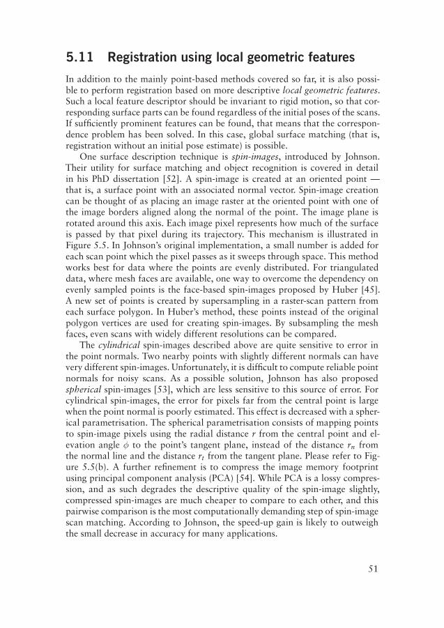
Three-dimensional records of objects and whole environments are an importanttool in several, and quite diverse, disciplines. One example is medical imaging,where three-dimensional (3D) images are used to show the inside of patients’bodies in a noninvasive way. Another one is archaeology, where 3D recordsof artifacts can be preserved without being damaged by an increasingly acidenvironment. 3D modelling also makes it possible to analyse objects in waysnot otherwise feasible. Yet another example is mobile robotics — the disciplinethat is primarily targeted by the work in this dissertation — where 3D scanningof the environment is useful for several subtasks, such as mapping, localisation,and extraction of semantic information from the robot’s environment.

3D scans can be represented in a number of ways. The central theme of thisdissertation is one such scan representation: the normal-distributions transform,or NDT. The normal-distributions transform transform provides an attractiverepresentation of range-scan data, which are normally available in the form ofunstructured point clouds. After applying NDT, the scanned surface is insteadrepresented as a piecewise smooth and continuous function with analytic first-and second-order derivatives. Such a representation of the data is advantageousin several ways.

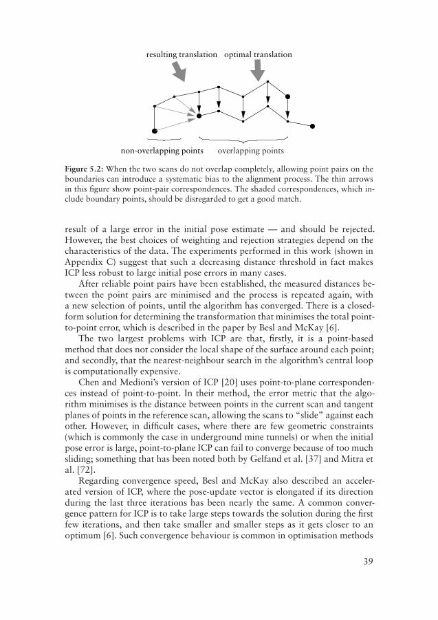
When performing 3D imaging, it is often the case that the whole area of in-terest cannot be captured in a single scan; be it because of occlusions, because itis too large, or because the object in question is fragmented in itself. Thereforeit is typically necessary to perform 3D scan registration — fitting the pieces to-gether — in order to produce a complete model. In order to align the piecewisescans (solving the jigsaw puzzle, so to speak) it is necessary to find the correctposition and orientation of each scan; that is, its pose. Finding the best pose isthe task of registration algorithms. Pairwise registration is the process of find-ing the pose that best aligns one scan with another, assuming that there is someoverlap between the surfaces of the two scans. Given an initial estimate of therelative pose difference between the two scans, local registration algorithms tryto improve that estimate. A good scan-registration algorithm should be robust

3

to large errors in the initial pose estimate and quickly produce a refined posethat precisely aligns the two scans. Scan registration is furthermore useful forpose tracking in mobile robotics. After registration, the precise position andorientation at which each scan was made are known, making it possible to re-cover the robot’s trajectory. Using the NDT representation of the scan data, itis possible to use standard methods from the numerical-optimisation literature,such as Newton’s method, to perform scan registration.

This dissertation mainly focuses on 3D scanning for mobile robots, and theprimary intended application is autonomous underground mining vehicles. Un-derground mining is, and always has been, a very dangerous enterprise. Peopleworking underground have had to endure many dangers. The risk of suffoca-tion, falling rocks, explosions, and gas poisoning are only a few examples. Min-ing is one of the jobs that are sometimes referred to as “triple-D tasks”: dull,dirty, and dangerous. The following quote from a Chinese miner is testamentto that:

If I’d been the boss in China, I wouldn’t allow people to work inmines. I would have them plant trees in the suburbs instead. [84]

Many steps have been taken to improve safety, but even today a large numberof lives are lost each year in mine accidents. In China alone, thousands of peo-ple are killed every year. According to official statistics from the Chinese stateadministration of work safety [21], no less than 8 726 people died in mine acci-dents in 2004 — that means an average of 23 persons per day! The death rateis horrifying, and the year 2004 was not unusual. The numbers are much lowerin the rest of the world, but safety for underground personnel in mines is stilla very important issue. Autonomous underground vehicles would be of greatbenefit to the mining industry, and 3D scanning is one important instrument inaccomplishing that goal. With 3D scan registration, it is possible to constructmetric 3D mine-tunnel maps with a minimum of human intervention. Such 3Dmodels can be used by future autonomous vehicles, and they are also useful forseveral practical purposes today, such as verifying that newly-built tunnels havethe desired shape compared to the original plans. In many countries the amountof material that has been removed from the ground must be documented andreported, and if a detailed 3D model of the mine exists, the volume is easyto measure. Scan registration may also be used for precise positioning whenperforming semi-automated rock-face drilling.

Localisation in underground mines is far from trivial. A naive way is touse dead reckoning from wheel odometry. However, the accuracy of odom-etry quickly deteriorates because of wheel slip and other inaccuracies. Deadreckoning can be improved by using an inertial measurement unit that mea-sures changes in pose with accelerometers and gyroscopes. But even then, theerror grows unboundedly over time. A common, and accurate, way of deter-mining positions in underground operations is to use triangulation with tripod-mounted total stations. Setting up and using a total station is excruciatingly

4

slow compared to the laser range finders commonly used in the robotics com-munity. It also requires someone to operate the device. Further options includeadding infrastructure to the environment; for example, in the form of magnetic“rails” or special beacons with known positions. A truly autonomous vehicleshould not be dependent on such modifications to the environment. When thevehicle is aboveground, it may be possible to use a global navigation satellitesystem, such as GPS. Underground, it is of course impossible to use navigationsatellites. Even for aboveground applications, such systems can be problematic.There are many places where it is hard to get a direct line of sight to a sufficientnumber of satellites, and when driving close to large buildings, satellite naviga-tion is often inaccurate because of indirect signal paths — the satellite signalsbounce off the walls. Instead of relying on any of these approaches, a vehiclethat is equipped with a 3D range scanner may instead use scan registration tomaintain an estimate of its pose, as described in this dissertation.

However, even with accurate scan registration techniques, pose errors willaccumulate over distance. Once the vehicle closes a loop and returns to a pre-viously visited location, it is possible to correct the pose estimate. The accu-mulated error may also be distributed over the covered trajectory, thus makingthe map consistent. The problem is how to reliably detect loop closure. Whenthe accumulated pose error is large, it is not possible to use the robot’s poseestimate to deduce that a loop has been closed. It may be necessary to detectloop closure from the appearance of scans, which means recognising a placejust by comparing its appearance to that of previous scans. While it is relativelyeasy for a human observer to recognise two scans acquired at the same place,it is not at all trivial to do so automatically with a computer. Detecting loopclosure by recognising a view is an example of the more general problem ofdata association: determining which inputs correspond to the same externalconditions. The normal-distributions transform provides a compact but still de-scriptive representation of 3D scans, which can be exploited to create a highlycompressed appearance descriptor that constitutes a formal representation ofthe appearance of a scan. Because of the high compression ratio, it is possible tocompare a vast number of scans in short time. Loop closure is detected when-ever two similar scans are found. This dissertation proposes an NDT-basedloop-detection method that is discriminative enough to successfully detect alarge part of scans that are acquired at the same place with a very low numberof false detections.

In order to enable more high-level tasks than scan registration, localisation,and mapping, it is desirable to extract semantic information from the available3D models. Having a truthful 3D map is one thing, but being able to automat-ically segment the map into meaningful components and “understand” whatthey represent will be necessary in order to further increase autonomy. Infor-mation that may be useful to extract in a mobile robot context includes walls,doors, and drivable surfaces. In an underground mining application, one impor-tant task where 3D surface analysis may be useful is boulder detection. Current

5

semi-autonomous mining vehicles are capable of following tunnels and dump-ing their load at specific sites. Autonomous loading of material, on the otherhand, largely remains an open problem. When confronted with a pile of ma-terial that is to be loaded into the bucket of the machine, it is in general notadvisable simply to dig into the pile blindly. In mines, there are commonly ob-stacles in the form of large boulders in the pile. In order to fill the bucket, it isnecessary to avoid any oversized boulders. This dissertation presents a method,also inspired by the NDT surface representation, that provides clues as to wherethe pile is, where the bucket should be placed for loading, and where there areobstacles.

1.1 Contributions

These are the main contributions of the present work:

3D-NDT surface representation. The 3D normal-distributions transform pro-vides a compact albeit expressive representation of surface shape withseveral attractive properties for use in registration, loop detection, andsurface shape analysis.

3D-NDT registration with extensions. Using the 3D-NDT surface representa-tion makes it possible to use standard numerical optimisation methodswith attractive convergence properties for scan registration. By using amultiresolution discretisation technique and trilinear interpolation, someof the discretisation issues present in the basic 3D-NDT registration algo-rithm can be overcome. With these extensions, the robustness of the reg-istration algorithm is substantially increased. 3D-NDT scan registrationwith the proposed extensions is shown to be more accurate and more ro-bust to poor initial pose estimates than current standard scan registrationmethods, and also to perform faster.

Colour-NDT registration. For registering scans based on surface shape, it isnecessary that their geometric structure provides sufficient constraints tofind an exact match. When the geometric features are insufficient, it is nec-essary to use other features of the scanned surface for registration. Colour-NDT is a kernel-based extension to 3D-NDT for exploiting colour infor-mation in order to accurately register coloured 3D scan data.

Appearance-based loop detection from 3D laser scans. The NDT surface rep-resentation can also be used to construct an appearance descriptor thatmakes it possible to perform fast loop detection by comparing histogramsof local surface orientation and shape.

Boulder detection from 3D laser scans. It is difficult in general to detect over-sized boulders in a pile of rock. A method inspired by NDT can be usedto analyse the surface structure of rock piles and guide an autonomous

6

loader so that it avoids such obstacles. The same method can potentiallyalso be used to extract drivable surfaces from 3D scans.

1.2 Outline

Following this introduction, Chapter 2 gives an overview of common conceptsthat are important to the rest of the text, including a more detailed descriptionof the registration problem, as well as notes on rotation representations andscan-subsampling strategies. Chapter 3 is a survey of range sensor hardware,discussing the advantages and disadvantages of different sensor modalities ina mine mapping application. Chapter 4 is a short reference of the platformsthat have been used to collect data for experimentally validating the proposedapproaches.

Part II is concerned with the problem of scan registration. Related workon registration is discussed in Chapter 5, after which the normal-distributionstransform (which is the main theme of this dissertation) and variants of it aredescribed in detail in Chapters 6 and 7.

Further applications of 3D-NDT for mobile robots are covered in Part III.Chapter 8 describes a novel approach to loop detection from 3D laser data,along with experiments to validate the effectiveness of the approach. Chapter 9shows a technique for surface-shape classification and how it can be used forboulder detection for an autonomous wheel loader.

The dissertation is summarised in Chapter 10, which also includes a discus-sion of current limitations and open problems as well as possible directions forfuture work.

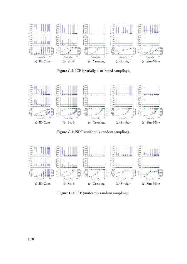
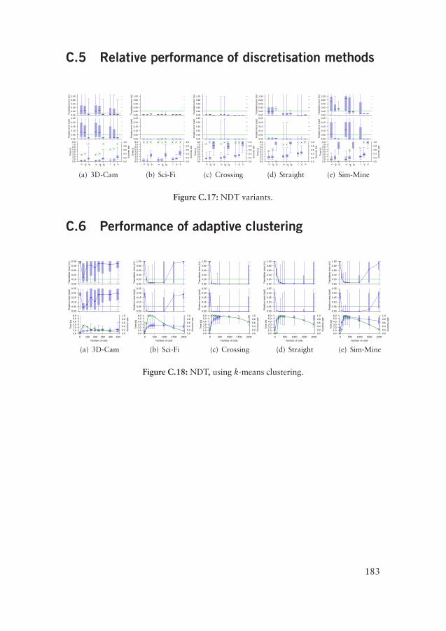
Finally, a brief reference of the notation used in this text is supplied in Ap-pendix A. Appendix B includes alternative 3D transformation functions for usewith 3D-NDT scan registration. Appendix C gives a more complete picture ofthe performed experiments by providing plots of the experimental results thathave been considered too bulky to include in the main text. A symbol index isincluded at the end.

1.3 Good-use right

Regarding the intended application that is targeted in this dissertation, it needsto be said (in accordance with the Uppsala Code of Ethics for Scientists [43])that there is a number of economical, social, and ecological concerns associatedwith the use of autonomous mining vehicles.

Clearly, there are many benefits of automating hazardous tasks, as statedwith emphasis in the previous text. Freeing humans from dangerous and dulltasks is, as phrased by Norbert Wiener [106], “the human use of human be-ings”. However — considering the current typical power balance between work-ers and employers, in the mining industry as elsewhere — the immediate effect

7

for miners when introducing autonomous vehicles will most likely not be im-proved work conditions and a healthier environment, but simply losing theirincome. Given that one of the main motivations behind this work is to improvethe quality of life for people in the mining industry, I believe that more researchon how to create a just and sustainable economic system is required for thesebenefits to be enjoyed by all involved parties.

The environmental effects (both in mining areas and on a global scale) ofincreasing the ore-extraction rate must also be considered before automatedmining systems are widely deployed.

It should also be noted that it is possible to use the results presented in thisdissertation for autonomous mobile robots in other, less beneficial, applications.I therefore include the following “good-use right” declaration:

It is strictly prohibited to use or to develop, in a direct or indirect way, anyof the scientific contributions of the author contained in this work by any armyor armed group in the world, for military purposes and for any other use whichis against human rights or the environment.

8

Chapter 2

Common concepts

2.1 Points, positions, and poses

In the following, scan points are often denoted by a vector ~x representing theirposition in space. A scan point may have many other properties as well, suchas colour and information about surface orientation, but the most interestingproperty in this context is usually its position, so ~x and the term “point” willoften be used interchangeably for a scan point and its position.

The concept of a pose is central to scan registration and localisation. Apose in this context is a combination of a position and an orientation. Morespecifically, a pose is represented by a rotation about the coordinate-systemorigin followed by a translation.

2.2 Notes on rotations

The representation of scan poses is central to scan registration. In two dimen-sions, translation can be straightforwardly represented as a 2D vector androtation as a scalar representing the counter-clockwise rotation angle. Three-dimensional translations can with the same ease be represented by 3D vectors.General rotations in 3D, however, are another matter. This section covers anumber of alternatives. Please refer to Altmann [1] for an exhaustive referenceon rotations or Diebel [27] for a more compact but thorough review.

2.2.1 3D rotation representations

Let’s consider the following 3D rotation representations:

Euler angles One of the most common 3D rotation representations is to usethree scalars, representing consecutive rotations around the three principal axes

9

x, y, and z. This is the so-called Euler-angle representation. For example, theEuler-angle vector

[φx, φy, φz] (2.1)

may represent a combined transformation where the scan is first rotated withangle φz around the z axis, then φy around the y axis, and finally φx around thex axis. The rotation sequence does not have to be z-y-x; arbitrary 3D rotationscan also be represented using the sequences x-y-x or x-z-x, for example.

Euler angles are relatively easy to understand and easy to implement. How-ever, using Euler angles as a representation of general rotation has some de-fects: mainly that Euler angles are not always unique, and that under certainconditions, they can lead to a situation called gimbal lock, where one degree offreedom is lost. Intuitively, gimbal lock can be understood by considering thatchanges in the first and third angles are indistinguishable when the second angleis at some critical value. For example, for a vehicle that is initially horizontal, ifthe rotation sequence is x-y-z and the second angle (pitch) is 90◦, the vehicle ispointing straight up. Then, the roll (rotation around the vehicle’s longitudinalaxis) and yaw (rotation around the vehicle’s vertical axis) are indistinguishable:gimbal lock has occured.

It is strategic to start with the largest rotation when using Euler angles.For mobile robot scan registration, the largest error is usually the yaw angle(around the vertical axis), which corresponds to the z rotation in this work.

Rotation matrices Arbitrary three-dimensional rotations can also be repre-sented as special orthogonal 3 × 3 matrices. Special orthogonal matrices havethe following properties: the transpose is equal to the inverse, and the determi-nant is equal to one. Multiplying two rotation matrices yields another rotationmatrix that represents the sequence of the original matrices applied in order. Infact, Euler angle rotations are commonly implemented as a product of threerotation matrices, one for each rotation axis. The Euler rotation example (2.1)can be expressed as the rotation matrix

RxRyRz =

cycz cysz −sy

sxsycz − cxsz sxsysz + cxcz sxcy

cxsycz + sxsz cxsysz − sxcz cxcy

, (2.2)

where ci = cosφi and si = sinφi.When using rotation matrices, it is important to make sure that they are

always orthogonal, an operation that can be relatively costly in terms of pro-cessing time. Due to numerical inaccuracies, the product of several rotationmatrices will inevitably drift from orthogonality. A nonorthogonal matrix nolonger represents rotation alone, but also a skew transformation that changesthe shape when applied to a point cloud.

Quaternions Quaternions provide a more compact representation than thenine numbers required for a rotation matrix. Quaternions are a 4D noncommu-

10

tative extension of the complex numbers, with one entry for the real part, andthree entries for the imaginary parts. To represent a rotation as a quaternion,the real part represents cos (φ/2) and the imaginary part represents~r · sin (φ/2),where φ is the angle of rotation and~r is a unit vector along the axis of rotation.

Quaternions are popular in the field of computer graphics, primarily be-cause they avoid the problem of gimbal lock and allow an easy way to expressinterpolations between rotations; for example, when distributing rotation erroramong a sequence of scans. A slight disadvantage of the quaternion representa-tion is that the values do not have any obvious meaning, like Euler angles do.A more severe problem is that quaternions used for rotation must be of unitlength. Normalising a quaternion is less expensive than making a 3× 3 matrixorthogonal. However, the unit-length constraint is problematic when quater-nions are included in the objective function of an optimisation problem. Theunit-length constraint is quadratic in form, and it is not always straightforwardto impose such a constraint when applying a numerical optimisation algorithm.

4D axis/angle Another representation is to use one scalar angle and a unit-length 3D vector describing the axis around which to rotate: (~r, φ). This repre-sentation is similar to quaternions, and it is straightforward to convert betweenthe axis/angle and quaternion representation:

(~r, φ)↔[

cos (φ/2)~r sin (φ/2)

]

. (2.3)

The axis/angle representation may be more intuitive than the quaternionbecause the axis and angle can be directly read from the values ~r and φ. Bothrepresentations are functionally equivalent. The problem with these two repre-sentations is that four variables are required, but 3D rotation only has threedegrees of freedom. The same rotation can be encoded using an infinite numberof rotation axes, as long as their directions are the same. Alternatively, the axismust be constrained to unit length.

“Rotation vectors” Recognising the extraneous parameter of the quaternionand axis/angle representation, 3D rotations can also be stored in a “rotationvector”, where the direction of the vector identifies the axis of rotation and thelength of the vector is proportional to the rotation angle. The rotation vectorrepresentation of rotating a vector around axis~r with angle φ is simply

φ~r, (2.4)

assuming that ‖~r‖ = 1.This representation, just like quaternions and the axis/angle representation,

avoids gimbal lock. Additionally, it requires no nonlinear constraint when usedin numerical optimisation. Even though this notation looks like a vector, ro-tations are not proper vectors: It is not possible to combine rotation vectors

11

using ordinary vector algebra. Instead, when combining two rotation vectors,one can convert both to quaternions, perform a quaternion multiplication, andconvert the result back to a rotation vector.

2.2.2 Summary

In the work on scan registration using 3D-NDT (in Chapter 6), Euler angleswith the sequence z-y-x will be used. The rationale for using Euler angles inthis case is to avoid incorporating a nonlinear constraint in the numerical opti-misation method. For the relatively small angles encountered when performingscan registration, gimbal lock is not likely to occur. Therefore the potentialdrawbacks of Euler angles are assessed to be outweighed by the easier problemformulation.

In the text, however, rotations will most commonly be described using theaxis/angle representation, because it is easier to understand and envision.

2.3 Registration

Pairwise registration is the problem of matching two scans when the relativepose difference between the scans is unknown. Given two scans with some de-gree of overlap, the output of a registration algorithm is an estimate of thetransformation that will bring one scan (which will be referred to as the cur-rent scan) into the correct pose in the coordinate system of the other scan (thereference scan), When the two scans match properly, they are said to be inregistration. (It is, however, not trivial to clearly define when two scans match“properly”. The problem of determining ground truth for registration will bediscussed in Chapter 6.)

In contrast to global surface-matching algorithms, the class of local regis-tration algorithms search locally in pose space, starting from an initial poseestimate given as input to the algorithm. Consequently, registration algorithmsmay find an incorrect transformation if the initial pose is far from the best one.The initial pose estimate can be selected manually or, in the case of a mobilerobot, can be determined from odometry data. If no prior information is avail-able, the initial pose estimate may simply be zero translation and rotation.

Scan registration can be used for pose tracking; that is, localisation by re-peatedly updating the robot’s pose estimate when the pose at a previous timestep is known. It can also be used for modelling. By registering a sequence ofscans, it is possible to construct a model of an object when it is not possible tocover the whole area of interest in one scan. If the “object” is large, such as anunderground mine, the “model” is a metric map of the environment.

Part II is devoted to scan registration.

12

2.4 Notes on sampling

When registering high-resolution scans, it is often practical to use only a subsetof the available scan points in order to improve execution speed.

Subsampling can be done in a number of ways. The simplest way is to useeither uniform subsampling, where every nth point from the scan is selected, orto pick a uniformly random selection of points. “Uniformly” in this case doesnot correspond to a uniform distribution of points, but to the probability ofselecting a certain point.

In many cases, not least when scanning in corridors and tunnels, the dis-tribution of points is very much denser near the scanner location than fartherout. If points are sampled in a uniformly random manner, the sampled subsetwill have a similarly uneven distribution. Few or no points may be sampledfrom important geometric structure at the far ends of the scan, resulting inpoor registration. To overcome this problem, it is common to use some form ofspatially distributed sampling in order to make sure that the sample density iseven across the whole scan volume. The way this has been done in the presentwork is by creating a grid structure with cells of equal size and placing thepoints of the scan in the corresponding cells. The cell size of this sampling gridis typically between 0.1 and 0.2 m. A random point is drawn from a randomcell until the required number of points is reached. If the distribution of cells isadequate, this strategy will give an even distribution of points.

Rusinkiewicz [89] has given an overview of different sampling strategies. Iftopology data in the form of mesh faces or surface normals at the points areavailable, it is possible to subsample in a more selective manner; for example,choosing points where the normal gradient is high or choosing points so thatthe distributions of normal directions is as wide as possible. The preferred strat-egy for choosing points varies with the general shape of the surfaces. Surfacesthat are generally flat and featureless, such as long corridors, are notoriouslydifficult to register accurately, but choosing samples so that the distributionof normals is as wide as possible forces the algorithm to pick more samplesfrom the features that do exist (bulges, crevices and the like), and may increasethe chance of finding a correct match. On the other hand, since many pointsare discarded in that kind of selective sampling, the registration becomes moresensitive to errors in the few remaining points.

Surface normals have not been computed for the point clouds used in thisdissertation, and therefore selective sampling based on curvature will not beused.

2.5 SLAM

Simultaneous localisation and mapping, or SLAM, is a central research topicin the mobile robotics community. It is an active research topic, and has beenfor many years now. Given a map, it is possible to perform localisation by

13

comparing observations from the world with the data in the map. Vice versa,if localisation can be provided (for example, from GPS), it is not difficult toconstruct a map by merging successive observations at their respective poses.However, performing localisation and mapping simultaneously is not at all triv-ial. It can be thought of as a “chicken or the egg” dilemma: which comes first,the map or the localisation capability?

One popular approach to the SLAM problem is to perform optimisation ona constraint network, or pose graph. A map can be represented as a pose graph,with local submaps at each node of the graph and edges connecting adjacentsubmaps. In graph-based SLAM solutions, the following steps are commonlyincluded:

1. registration,

2. pose-covariance estimation,

3. loop detection,

4. relaxation.

Successive views from the robot are registered in order to track the pose of therobot (localisation) and build a metric map (mapping). For each view (or forsubmaps generated from a set of views), a node is inserted into a scene graph,with an edge connecting the current submap to its neighbours. A covariance es-timate of the relative pose between neighbouring submaps is also required, andis attached to the edges of the graph. Once the robot detects that it has returnedto a previously visited place, the error that has accumulated over the traversedloop can be computed. The map is reformed to a consistent state by performingrelaxation of the graph, based on the covariance estimates associated with eachedge.

There are also other approaches to solving the SLAM problem; see, for ex-ample, the much-cited SLAM review of Thrun [102]. Frese et al. [34] have pub-lished a multilevel relaxation algorithm for graph-based SLAM. Their articlealso nicely describes the problem and related approaches. Much more informa-tion on SLAM and methods to solve it can be found in the Springer Handbookof Robotics [93].

The first two items in the list above will be addressed primarily in Chapter 6,and a method for 3D loop detection is proposed in Chapter 8. Pose-graph re-laxation is not directly addressed in this dissertation. Please refer, for example,to the 3D relaxation methods of Grisetti et al. [42] and Borrman et al. [10]instead.

14

Chapter 3

Range sensing

This chapter describes how to acquire the range data needed for metric 3Dmapping. There are several types of measuring devices that can be used forscanning and creating a 3D model of a scene. The following text is an overviewof some common range measurement principles and a discussion on their utilitywith the primary perspective of modelling an underground mine system.

For other in-depth references to sensors, please refer to the books by Ev-erett [30] or Webster [105].

3.1 Range sensors

Most of the sensor types discussed in this section are based on the same prin-ciple: sending out an energy beam of some sort and measuring the reflectedenergy when it comes back. They have several properties in common. They areall vulnerable to the effects of specular reflection to some degree.

Most surfaces are diffuse with respect to visible light; that is, they reflectincoming light in all directions. For a perfectly diffuse surface, the intensity ofthe reflected energy is the same from all viewing angles, and is proportional tothe cosine of the angle of incidence. The more specular, or shiny, a surface is,the more of incoming energy is reflected away in an angle equal to the angleof incidence. This effect can be seen when pointing the beam of a flashlighttowards a mirror, which is a highly specular surface for visible light. The litspot on the mirror itself is barely visible, because almost all light is deflected ina specular fashion, but when looking at a nearby wall, the spot of light showsup clearly because the wallpaper is diffuse. The proportions of specular anddiffuse reflection for a given surface depend on its microscopic structure, andare different for different wavelengths. The longer the waves of the incomingenergy, the rougher the surface has to be in order to be a diffuse reflector. Asan analogy, one can imagine throwing a ball at a structured surface, as in Fig-

15

φ φ φφ φ

SpecularDiffuse

φ

Figure 3.1: The same surface can be both a specular and diffuse reflector, dependingon the wavelengths of the incoming energy. The images on the bottom row illustrate aperfectly diffuse, a moderately specular, and a perfectly specular surface, respectively.

ure 3.1. A large ball will bounce away (specular reflection), while a smaller ballis more likely to bounce back, or in some other direction (diffuse reflection).1

Specular reflection can lead to serious misreadings. For example, if the beambounces off a wall at a shallow angle, the sensor’s maximum distance will bereported instead of the actual distance to the wall. Or, if the beam originatesfrom point A, bounces off object B and then is reflected diffusely from object Cback to the sensor, the measured distance will be (A→ B→ C→ A)/2 insteadof A→ B.

In general, a shorter wavelength leads to higher range resolution (more ac-curate range readings) and less specular reflection (less missing readings fromshiny surfaces) but a shorter maximum range due to absorption and scattering(attenuation). Gas and particles in the air absorb and scatter the energy, makingless of the beam return to the receiver, consequently decreasing the reliability ofthe measurement.

Instead of having a single sensor which is rotated to scan the full environ-ment, it may be tempting to use multiple sensors measuring simultaneously indifferent directions to increase the scanning rate. Doing so can result in prob-lems with crosstalk — bounced or direct impulses from nearby sensors — ifthe sensors are not properly shielded or the environment is highly specular.Crosstalk effects are especially pronounced in confined spaces.

1These examples are taken from Everett [30].

16

3.1.1 Radar

The term radar is an acronym for “radio detecting and ranging”, and has tradi-tionally been used for range-finding devices that use radio waves. However, in1977 the IEEE redefined it so as to include all electromagnetic means for targetlocation and tracking [30]. Nevertheless, this section only considers radio waverange finders.

Perhaps the most well-known application of radars is for military vessels atsea or in the air. When used on ships or airplanes, the goal is to detect the loca-tion and bearing of far away objects in a mostly empty space, which is an appli-cation where radar performs especially well. Because radar uses comparativelylong wavelengths, it can be used over very long ranges, although the resolutionis poor compared to sensors with shorter wavelengths. Furthermore, radar isnot vulnerable to dust, fog, rain, snow, vacuum, or changing light conditions.A unique feature of radar is that it can detect multiple objects downrange. Itdoes not penetrate steel or solid rock, however.

In a mine tunnel setting, there are several drawbacks of using radar for de-tailed model building. Radar wavelengths are very long in comparison to laserrange finders. This means that the maximum angle of incidence is rather lim-ited. In a tunnel environment, the long wavelength puts a limit on the distanceahead where the tunnel wall can be accurately measured.

Another possible limitation is the potentially large piece of hardware neededfor an accurate radar. For precise modelling, a narrow so-called pencil beam isrequired. The resolution depends on the wavelength of the emitted beam aswell as the aperture of the antenna. The beam width is inversely proportionalto the antenna aperture for a given frequency. Using millimetre-wave radar, itis possible to get high resolution with a relatively small aperture, at the expenseof range, but very narrow beams still require impractical antenna sizes for ourapplication. At 77 GHz, which is a common millimetre-wave radar frequency,a 1◦ beam requires an aperture of 224 mm [31]. Larger apertures would makeit difficult to mount the antenna on a mining vehicle.

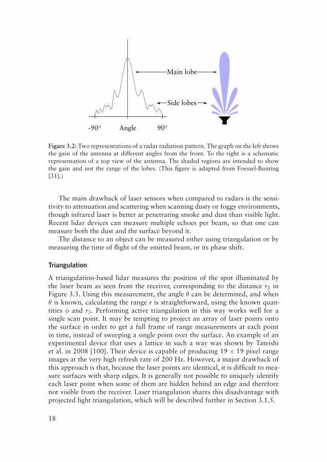
Unfortunately, a single narrow beam is impossible to achieve in practice.The radiation pattern always includes a number of side lobes — less intensebeams that spread out around the main beam (see Figure 3.2). The reflectionsof these lobes will interfere with the main signal and lead to noisier results, notleast in confined spaces, where all lobes will reflect off of nearby surfaces.

3.1.2 Lidar

Range-sensing devices using laser are commonly referred to as lidars: “lightdetecting and ranging”, or ladars: “laser detecting and ranging”. In this text,laser range finders will be called lidars, or simply laser scanners.

In contrast to the beams of radars and sonars, a laser beam can be madehighly focused, without side lobes. This is also an effect of the short wavelength.

17

��

Main lobe

Angle-90◦ 90◦

Side lobes

Figure 3.2: Two representations of a radar radiation pattern. The graph on the left showsthe gain of the antenna at different angles from the front. To the right is a schematicrepresentation of a top view of the antenna. The shaded regions are intended to showthe gain and not the range of the lobes. (This figure is adapted from Foessel-Bunting[31].)

The main drawback of laser sensors when compared to radars is the sensi-tivity to attenuation and scattering when scanning dusty or foggy environments,though infrared laser is better at penetrating smoke and dust than visible light.Recent lidar devices can measure multiple echoes per beam, so that one canmeasure both the dust and the surface beyond it.

The distance to an object can be measured either using triangulation or bymeasuring the time of flight of the emitted beam, or its phase shift.

Triangulation

A triangulation-based lidar measures the position of the spot illuminated bythe laser beam as seen from the receiver, corresponding to the distance r2 inFigure 3.3. Using this measurement, the angle θ can be determined, and whenθ is known, calculating the range r is straightforward, using the known quan-tities φ and r3. Performing active triangulation in this way works well for asingle scan point. It may be tempting to project an array of laser points ontothe surface in order to get a full frame of range measurements at each pointin time, instead of sweeping a single point over the surface. An example of anexperimental device that uses a lattice in such a way was shown by Tateishiet al. in 2008 [100]. Their device is capable of producing 19 × 19 pixel rangeimages at the very high refresh rate of 200 Hz. However, a major drawback ofthis approach is that, because the laser points are identical, it is difficult to mea-sure surfaces with sharp edges. It is generally not possible to uniquely identifyeach laser point when some of them are hidden behind an edge and thereforenot visible from the receiver. Laser triangulation shares this disadvantage withprojected light triangulation, which will be described further in Section 3.1.5.

18

r2

θ

r

Receiver

Transmitter

r3

φ

Figure 3.3: Active triangulation. The range r is measured by deducing the angle β fromr2 and the known quantities φ and r3.

Interest from the car industry is leading the pressure for cheaper laser rangefinders, and a recent example with very low production cost, aimed at the con-sumer market, has been presented by Konolige et al. [59]. Their lidar acquiresa 360◦ planar scan with 1◦ resolution at 10 Hz with 3 cm accuracy out to 6 mdistance. The hardware cost is listed at no more than 30 USD (2008). The sen-sor consists of a 10 cm wide housing that contains a rotating block on which alaser module (using visible red light) and a CMOS imaging sensor are mounted.Included is also a digital signal processing unit for subpixel interpolation. Usinga revolving block instead of a fixed laser diod shining at a rotating mirror (asis common for the time-of-flight lidars that will be mentioned shortly) makesit possible to miniaturise the sensor and therefore reduce the cost. However,because of the short maximum range, it is not useful in a mining application.

Time of flight

Another method for lidars is to emit rapid laser pulses and deduce the range bymeasuring the time needed for a pulse to return. Assuming that the laser travelsthrough a known medium (such as air), measuring the distance is possible usingtimers with very high resolution. This is a very accurate method, but also quiteexpensive due to the electronics required.

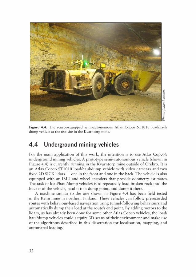
A prominent example of time-of-flight lidars are the SICK LMS laser scan-ners, commonly used in the mobile robotics community. The SICK scanners are2D sensors by design, sweeping a laser point to produce a 180◦ planar rangescan. Mounting a planar range scanner on a pan/tilt unit makes it possible toacquire 3D scans. Such 3D scanning devices have been used in many roboticresearch applications [4, 75, 77, 79, 98], as well as in this work. An exampleof this kind of setup can be seen in Figure 3.4. Depending on the configurationof the pan/tilt unit, the scan can be either pitching, rolling, or yawing; as de-scribed by Wulf and Wagner [107]. The different configurations are shown inFigure 3.5.

More recently, time-of-flight lidars that are designed to produce 3D scanshave become available, such as the Velodyne HDL-64E. This sensor uses a verti-

19

Figure 3.4: A SICK LMS 200 lidar, mounted on a pan/tilt unit to produce 3D scans.

(a) Pitching scan

(b) Yawing scan

(c) Rolling scan

Figure 3.5: 3D scanning methods for 2D lidars, showing how the lidar is actuated andthe density of the resulting point cloud. (This figure is reprinted from the original paperby Wulf and Wagner [107].)

20

wm

r

x

Transmitter

Receiver

Figure 3.6: Phase shift measurement: x is the distance corresponding to the differentialphase φ. This figure is adapted from Everett [30].

cal array of 64 lasers so that the sensor’s vertical field of view is approximately25◦. The whole unit revolves, producing a full 360◦ horizontal field of view.The accuracy and range resolution of the Velodyne scanner matches the SICKlidars, but because of the use of multiple lasers the data rate is vastly higher.The Velodyne HDL-64E produces over 1.3 million distance measurements persecond and omnidirectional 3D scans at up to 16 Hz. Getting 3D laser dataat such high rates is very attractive for mobile robot applications, and severalof the participants in the 2007 DARPA Urban Challenge used this device. Atpresent the cost of the Velodyne lidar (75 000 USD in 2006) prevents its usein many applications, but in the near future full-3D lidars are likely to becomemore common.

Phase shift

The phase shift of the incoming beam compared with the outgoing beam canalso be used to determine the distance to the closest surface, as illustrated inFigure 3.6. The phase shift of the actual light waves is typically not measured,but the light is modulated with a given frequency and the phase shift of themodulated signal is measured. Using a lower modulation frequency effectivelyincreases the maximum range without any negative effects from increased spec-ular reflection. If the measured shift in phase between the transmitted and thereceived signal is φ, the distance r to the target surface can be formulated as

r =φwm

4π=

φC

4πfm(3.1)

where wm is the modulation wavelength, C is the speed of light and fm is themodulation frequency [30]. The phase shift can be measured by processing thetwo signals and averaging the result over several modulation cycles.

One important negative aspect of using phase shift is that there is a maxi-mum range given by the modulation frequency after which the signal “wrapsaround”. For example, as long as a single beam is used, it is not possible to re-

21

��

��

measuredrange

desired range

Figure 3.7: Wrong range measured because of sonar-beam spread (the spread of thesonar beam is somewhat exaggerated in this figure).

liably tell the difference between an object located wm + 0.1 m from the sensorand one which is only 0.1 m or 2wm + 0.1 away.

3.1.3 Sonar

Sonar sensors are similar to radars and lidars, but measure the time of flight ofsound pulses instead of radio waves or light.

Traditionally, sonars have mostly been used for underwater applications,such as submarines or fishing equipment. Since the speed of sound is greaterin water the wavelength is longer, and thus the range resolution is not as goodas that of a wave with the same frequency in air. But the main advantage ofunderwater sonar is its range capacity. Water, being virtually incompressible,allows sound waves to travel hundreds or even thousands of kilometres.

Sonars are inexpensive, but it is often difficult to get accurate range readingsusing sonars. The nature of sound waves makes it difficult to focus a soundbeam. The resulting lack of angular resolution disqualifies sonar for detailed3D modelling, but can be an advantage when using sonar as a safety measure,to detect people in the vicinity of the vehicle. The large spread of the beamalso affects the range resolution: When the beam hits a surface at a shallowangle, the measured distance is shorter than the true distance, as illustrated inFigure 3.7.

Because of the low production cost, sonars are popular in robotic applica-tions with lower demands on accuracy, and for obstacle avoidance.

3.1.4 Stereo vision

In contrast to most of the previously discussed sensor types, with stereo visionit is possible to produce a full two-dimensional range image at once.

Stereo 3D sensing uses two parallel cameras, and exploits one of the effectsused by humans to recognise depth. Stereo vision uses passive triangulationto compute a range image. First, a point of interest is located in one image.A common method for picking interesting points is to use the scale-invariantfeature transform (SIFT, [61]) in order to locate pixels whose surrounding tex-ture makes it possible to reliably recognise them from multiple viewpoints. The

22

same point is recognised in the other image, based on the surrounding texture.Then, the distances of both points are measured with respect to some commonreference, and the range is calculated using the angles which can be derivedfrom these distances, just as for active triangulation (Figure 3.3).

Not all pixels in the camera image can be used for range measurements,only the ones that are recognisable as features, and therefore the attainableresolution for stereo vision is limited and context dependent. In a low-contrastenvironment, only a small number of points are possible to extract from eachimage.

Another problem is that the range accuracy decreases with the distance tothe measured surface and increases with the baseline length. The baseline is thedistance between the two cameras. Because the measured point must be seen byboth cameras, the sensor will be blind at the closest range, unless the camerascan verge (so that the sensor can “cross its eyes”), and this minimum distanceincreases with the baseline length. So a stereo-vision sensor that aims to beaccurate for long distances (several metres away) will not be able to measurethings that are close to the sensor.

Although the input rate of stereo vision is high and the hardware is both in-expensive and simple, the disadvantages mentioned above are problematic. Themain problems are that range accuracy is worse than that of electromagneticrange finders and that untextured surfaces are difficult or impossible to mea-sure, because there is no good way of recognising corresponding points fromthe two camera viewpoints [45].

3.1.5 Projected-light triangulation

Yet another method for 3D scanning is to project a light pattern onto the sceneand analyse the shape of the pattern as seen by a video camera. This is anotherexample of active triangulation. Several different patterns are mentioned in theliterature. Some examples include a bar code of sorts, with alternating blackand white parallel stripes of different widths, a wedge, or a continuous colourgradient [57, 90]. The projected pattern is observed by the camera, and thestripes are identified in the resulting image. For each pixel, the distance is deter-mined with triangulation between the pixel viewing ray and the correspondingplane of light emitted by the projector. The resolution depends on the patternand the resolution of the camera. If a stripe pattern is used, only points alongthe stripe borders can be measured. If a continuous gradient is used, the fullresolution of the camera can be used, but only if the surface is single-coloured.

One drawback when scanning scenes as large as mine tunnels is the diffi-culty of getting sufficient edge sharpness for the light pattern. To get a brightimage, the diameter of the projector lens must be large when using conven-tional projector methods. A large diameter leads to a shallow depth of fieldof the projected pattern: It will only be sharp at a specific distance from theprojector.

23

If a fixed stripe pattern is used, it is difficult to use projected-light triangula-tion for surfaces with discontinuities. The reason is that it is difficult to identifya certain stripe when it “jumps” between the two sides of an edge. This diffi-culty can be overcome by using a series of alternating patterns. Then, each pixelis identified by observing how it changes from light to dark over time, insteadof identifying it from the light pattern showing in the neighbouring pixels. Eachstripe has a unique on-off pattern, and the stripe can be identified by observingits history over the last few frames. This way, discontinuous and moderatelytextured surfaces can be measured, but the method is on the other hand likelyto fail if the object or sensor moves. This rules out using it for navigation or ona moving vehicle.

3.1.6 Time-of-flight cameras

A new type of range sensor that has only become available in recent years are so-called time-of-flight cameras. Even though the common term for these sensorsis time-of-flight cameras, they do in fact measure phase shift. The working prin-ciple of these cameras is to illuminate the scene with modulated near-infraredlight using an array of LEDs. The camera computes a range value for each pixelof the image based on the phase shift of the incoming modulated light and alsorecords the reflectance. The result is two images: one grey-scale image from thereflectance values and one depth map with a full frame of range values.

The key advantage of time-of-flight cameras compared to lidars is that theyproduce a full frame of range measurements (typically up to 160 × 120 pixelsfor current models) at almost normal video frame rates (around 15 Hz). Forthe PMD[vision] 19k sensor, which was used for some of the work in thisdissertation, the data rate is around 288 000 points per second, compared to13 000 for the SICK LMS 200 lidar, which must also be rotated to see morethan a single scan plane. In addition to the high data rate, another advantageof time-of-flight cameras is that the hardware is relatively inexpensive.

There are several drawbacks, however, that currently prevent the use oftime-of-flight cameras for underground localisation and mapping. One is thatthe noise level of the sensors is significant. Elaborate methods are required tofilter the output data as well as to calibrate the camera in order to avoid sys-tematic errors. Recently, several research groups have published methods forcalibration and noise filtering of time-of-flight cameras [49, 71]. The sensorsare also sensitive to the amount of background illumination compared to thestrength of the camera’s active illumination. There are presently no availablemodels designed for outdoor use, although such sensors can be anticipated. Yetanother problem is to find a proper exposure time. With a too short exposuretime, not enough light will be recorded from farther surfaces. With a too longexposure time, nearby or light-coloured surfaces will get over-saturated, result-ing in “holes” in the range data. Furthermore, the risk for motion blur increaseswith a longer exposure time. One way to deal with the exposure-time problemis to use multiple exposures. Perhaps the most severe drawbacks with respect to

24

mine mapping are the limited field of view and the short maximum range. Forthe PMD[vision] 19k, the maximum range is 7.5 m and the viewing angle is 40◦,compared to at least 30 m and 180◦ for common lidars. It would, of course, bepossible to fit the camera with a more wide-angle lens in order to cover a largerfield of view, but the problem is the infra-red illumination. It is difficult andexpensive to illuminate a larger part of the scene. A very high-powered LED ar-ray would be required. With a brighter LED array, the maximum range couldpotentially be higher and the sensitivity to background illumination lower. Still,as with phase-shift lidars, the maximum range is also governed by the phaseshift wrap-around effect. Using multiple light sources with different modula-tion wave lengths, it may be possible to overcome the wrap-around problem tosome extent.

As the technology matures, we can hope that future time-of-flight cameraswill overcome most of these limitations. As of today, these sensors are not usefulfor underground localisation and mapping.

3.1.7 Summary

It seems quite clear that only lidars will produce scans with enough accuracyand range to be used for mine-tunnel profiling; the main advantages being highaccuracy and resolution and also the relatively low sensitivity to specular re-flection. However, if the difficulties of time-of-flight cameras can be overcome,they pose a promising solution for the future.

However, none of the methods discussed in this dissertation are restrictedto any particular type of sensor. Any sensor that can produce an unstructured3D point cloud may be used. For using Colour-NDT (Chapter 7), a colourcamera that is calibrated for use in coordination with a 3D range sensor is alsorequired.

3.2 Scanning while moving

Lidars have very good accuracy and range characteristics, but making a full3D scan takes a few seconds, because the laser beam has to be swept overthe whole scene. Therefore a common mode of collecting scan data in mobilerobot applications is to stop the robot while the scan is being made. For anautonomous mine vehicle, it is not acceptable to stop every few metres to makea scan. It is necessary to be able to perform 3D scanning while moving, withouttoo much noise in the scan data.

If the vehicle moves slowly over a flat surface and the wheel odometry isreliable over the short distance covered while making the scan, the motion dur-ing scanning can easily be compensated for using only the odometry. However,wheel odometry is notoriously inexact, and especially so while the vehicle isturning. With the help of an inertial measurement unit (IMU) the odometry canbe made slightly more reliable. An IMU contains 3D accelerometers and gyros

25

to measure the translation and rotation in 3D-space. Using an IMU makes itpossible to compensate for vertical movement and pitch and roll rotations tosome extent, although IMUs also suffer from noise and sensor drift. It wouldbe interesting to investigate to what extent the motion of a mine vehicle in arealistic scenario can be filtered using an IMU and if such filtering is enough toget acceptable 3D scans while moving.

One approach for correcting laser scans under general vehicle motion with-out relying on expensive sensors has been presented by Harrison and New-man [44]. Their method assumes that vertical planes can be found in the scan.The exact trajectory of the robot while the scan was made is recovered by mak-ing near-vertical planes perfectly vertical. The method has been shown to workwell in an outdoor campus environment. Unfortunately, walls that are unevenand only nearly vertical are common in underground mines and other unstruc-tured environments, so the method of Harrison and Newman cannot be usedthere.

An interesting method for compensating for motion while scanning wasrecently published by Stoyanov and Lilienthal [97]. Using a SICK 2D lidar spin-ning around the vertical axis (thus performing yawing scans, as depicted in Fig-ure 3.5), their method exploits the fact that after each revolution of the scanner,it should re-observe a part of the scene. ICP scan registration (which will be de-scribed in Section 5.1) on the scan points that correspond to the same surfacecan be used to find the accumulated pose error between the start and end ofthe scan, after which the multilevel relaxation algorithm of Frese et al. [34] isused to distribute the error over the scan. Currently the method of Stoyanovand Lilienthal is limited to planar motion (assuming a flat floor). It would beinteresting to see how it can be extended to the fully three-dimensional casewith six degrees of freedom.

Bosse and Zlot [15] also recently presented a promising method for contin-uous 3D scan registration with a spinning 2D laser. A remarkable property ofthe method of Bosse and Zlot is that they use only laser data and require noodometry or IMU information. The experimental platform used in their workis equipped with a SICK lidar mounted on a spinning platform to producerolling 3D scans at a speed of 2 Hz. Their approach is based on an interestingscan-registration technique that shares some properties of the ICP and NDTalgorithms, which will be covered in Chapters 5 and 6. Instead of matchingpoints directly, Bosse and Zlot construct a 3D grid and estimate local surfacedescriptors from the surface within each grid cell in the form of ellipsoids. (Theellipsoids are essentially the same as the Gaussian functions used by NDT.)They further compute eccentricity parameters showing how planar, linear, orspherical the ellipsoids are in a fashion similar to the method for loop detec-tion that is described in Chapter 8. The timestamp of each scan point is alsorecorded in the data structure that is used for registration. Standard scan regis-tration tries to find the relative pose between two scans. The method of Bosseand Zlot instead tries to find the trajectory during one scan. The time spent

26

for making a scan is discretised into separate time steps. The ellipsoids in thecurrent scan are grouped based on their timestamp. The algorithm iterativelytries to find the best pose for the group of ellipsoids associated with each timestep. The ellipsoids that were measured close to a certain time step should, as agroup, match some of the ellipsoids of the reference scan. The estimated posesat each sampled time step are used to compute an interpolated cubic spline forthe continuous trajectory, which is then used to correct the scan.

With the advent of general-purpose methods that can correct 3D scans madeby tilting or rotating 2D lidars under general vehicle motion, it is likely that themain limitation of such range sensors — their low data acquisition speed — canbe overcome. It can therefore be expected that such relatively inexpensive sen-sor setups will continue to be common in the mobile robot research communityand also be useful in industrial production environments. Looking beyond thenearest time horizon, it seems likely that fully-3D lidars, such as the Velodyne,or new generations of time-of-flight cameras will be the 3D range sensors ofchoice.

The methods proposed in the later parts of this dissertation do not dependon the way in which the 3D point clouds are acquired, as long as there is asensor setup that produces scans without too much distortion.

27

Chapter 4

Platforms and environments

Before continuing to the main parts of the dissertation, let’s take a moment tohave a look at the experimental platforms used for data collection and experi-mental validation in the following chapters, as well as the vehicles and environ-ments of the intended mining application.

4.1 Tjorven

Tjorven is an ActivMedia Pioneer P3-AT equipped with an onboard computerand an array of sensors. This robot has been used for various mapping projectsat the AASS research institute. Tjorven is shown in Figure 4.1. The sensorsthat are relevant for this work are a SICK lidar mounted on a pan/tilt unit andwheel encoders that provide 2D odometry. The pan/tilt unit enables Tjorven tocreate pitching 3D scans with 180◦ horizontal and about 100◦ vertical field ofview. Other sensors include an omnidirectional camera and a differential GPSantenna. For the work on registration of coloured point clouds (Chapter 7), aPMD[vision] time-of-flight camera was mounted on top of the laser scanner.

The names of the robot platforms at AASS are all taken from the children’sstories of Astrid Lindgren. Tjorven is the name of a rather plucky girl in thestories about the people of Saltkråkan (“Seacrow Island” in English).

4.2 Alfred

Alfred (Figure 4.2) is a custom robot platform based on a Permobil electricwheelchair. The hardware was set up by a group of students from HalmstadUniversity (Högskolan i Halmstad). On top of the basic hardware platform is aSICK lidar, mounted on a continuously rotating motor with slip-ring contactsthat makes it possible to create omnidirectional (yawing) 3D scans. A Hokuyo2D lidar, used for providing 2D localisation, is also mounted on Alfred. The

29

(a) Standard setup. In addition to the laserscanner used for 3D mapping, Tjorven is alsoequipped with a digital camera, an array of

sonars, and a differential GPS system.

(b) The sensor setup used in thecolour-registration experiments. The

time-of-flight camera is mounted on top of theSICK laser scanner.

Figure 4.1: Tjorven.

body of the robot can be raised and lowered using a hydraulic lift mechanism.Alfred was used to collect some of the data used for loop detection in Chapter 8.

The name Alfred is taken from the farmhand in the Astrid Lindgren booksabout Emil. Alfred is big, strong, and kind; much like the electric wheelchairused in this platform.

4.3 Kurt3D

The robot Kurt3D of Osnabrück University (shown in Figure 4.3) was used forcollecting some of the data used for the work on place recognition in Chapter 8and the performance comparisons of ICP and NDT in Section 6.4.2.

Kurt3D is a relatively high-speed mobile robot platform, moving at a con-trolled pace of up to 4 m/s (14 km/h). The motors allow for speeds up to 5.4 m/s(19 km/h), but the current computer hardware and algorithms can not controlit reliably at such speeds. The robot is equipped with a SICK laser scanner aswell as two digital colour cameras.

The 3D range sensor on Kurt3D is, similarly to Tjorven, a tiltable 3D laserscanner. A small servo motor has been attached to the scanner to perform acontrolled pitch motion. The field of view and other scanner characteristics arevery similar to those of Tjorven.

30

Figure 4.2: Alfred.

Ph

oto

:C

hri

sto

ph

erL

örk

en.

Figure 4.3: Kurt3D in the Kvarntorp mine.

31

Ph

oto

:Jo

han

Lar

sso

n.

Figure 4.4: The sensor-equipped semi-autonomous Atlas Copco ST1010 load/haul/dump vehicle at the test site in the Kvarntorp mine.

4.4 Underground mining vehicles

For the main application of this work, the intention is to use Atlas Copco’sunderground mining vehicles. A prototype semi-autonomous vehicle (shown inFigure 4.4) is currently running in the Kvarntorp mine outside of Örebro. It isan Atlas Copco ST1010 load/haul/dump vehicle with video cameras and twofixed 2D SICK lidars — one in the front and one in the back. The vehicle is alsoequipped with an IMU and wheel encoders that provide odometry estimates.The task of load/haul/dump vehicles is to repeatedly load broken rock into thebucket of the vehicle, haul it to a dump point, and dump it there.

A machine similar to the one shown in Figure 4.4 has been field testedin the Kemi mine in northern Finland. These vehicles can follow prerecordedroutes with behaviour-based navigation using tunnel-following behaviours andautomatically dump their load at the route’s end point. By adding motors to thelidars, as has already been done for some other Atlas Copco vehicles, the load/haul/dump vehicles could acquire 3D scans of their environment and make useof the algorithms described in this dissertation for localisation, mapping, andautomated loading.

32

4.5 Kvarntorp

Several of the data sets used for evaluating the methods proposed in this dis-sertation were collected in the Kvarntorp mine. The Kvarntorp mine is locatedsouth of Örebro in Sweden. This mine is no longer in production, but was onceused to mine sandstone. The mine consists of slightly more than 40 km of tun-nels, all in one level. Parts of the mine are currently used as archives and storagefacilities, while others are used as a test bed for mining equipment.

Because of the excavation technique used in sandstone mines, the tunnelshave a rather characteristic shape with flat ceiling and straight walls, whereasother underground mine tunnels have more rounded and often much narrowertunnels. Parts of the mine that are used as a test site for mining vehicles haveartificial walls erected along some tunnels, used to simulated narrower tunnels.

Even though the floor and ceiling are relatively flat, the unevenness of thefloor makes a wheeled vehicle tilt considerably while driving over it. The rough-ness is comparable to that of a gravel road. Therefore, using 2D techniquesinstead of the 3D algorithms used in this work (thereby disregarding tilt anglesand changes in floor height) inevitably leads to errors.

33

Part II

Scan registration

Chapter 5

Related work on scanregistration

Scan registration is an important process in several areas. It is used for con-structing models from partial scans in disciplines as diverse as medical imag-ing, archaeology, and robotics. It is also useful for enabling mobile robot self-localisation. It is a subject that has received considerable attention in the past,and continues to do so. This chapter covers some relevant previous work onscan registration. The NDT scan-registration algorithm, which constitutes oneof the main topics of the thesis, will be described further in Chapter 6. Relatedvariants of the NDT algorithm will be addressed in Section 6.5. Chapter 7 isconcerned with registration of coloured 3D point clouds. Related work specificto coloured data will be covered in Section 7.1.

5.1 ICP

The iterative closest point (ICP) algorithm is widely used today for registrationof 3D point clouds. The two seminal papers on ICP were written by Besl andMcKay [6] and Chen and Medioni [20]. Since its conception, a large numberof variants have been developed. A good survey of different variations of ICPwas presented by Rusinkiewicz [89]. To summarize the algorithm concisely:ICP iteratively refines the relative pose of two overlapping scans by minimisingthe sum of squared distances between corresponding points in the two scans.Corresponding point pairs are identified by the point-to-point distance.

The first step is to find corresponding point pairs in the current scan andthe reference scan. For each point in the current scan, the chosen correspondingpoint is its closest neighbour (by Euclidean distance) in the reference scan. Abasic limitation of ICP is that the nearest neighbour point does not in generalcorrespond to the same point on the scanned surface, especially if the two scansare far apart. In successful applications of ICP, it nevertheless converges to a

37

Figure 5.1: Registering two scans from a mine tunnel using ICP. The yellow scan isbeing matched to the dark green scan. The point-to-point correspondences are shownwith bright green arrows.

useful solution, given its iterative nature. The search for nearest neighbours iswhere most of the execution time is spent. The pairing of closest points at oneICP iteration is illustrated in Figure 5.1.

It can be beneficial to weight the point pairs, assigning more weight to cou-ples that are more likely to correspond to the same surface points. A reason-able weighting criterion may be to set the weight inversely proportional to thepoint-to-point distance, so that points further apart have lower weights thanpoints with close neighbours. However, for tunnel or corridor data, such linearweighting can degrade performance. Because most points along the walls andceiling will generally be well-aligned, their influence will overwhelm point pairswith larger distances, which correspond to corners and other features that areimportant for acquiring a good match.

In addition to any weighting performed, some outlier pairs should also berejected entirely. Point-pair rejection can be seen as a special case of point-pairweighting. A common criterion is to reject all point pairs with a distance abovea certain threshold. Additionally, point pairs that include a boundary pointfrom the reference scan should always be rejected. Otherwise, points from non-overlapping sections of the data may cause a systematic “drag” bias — seeFigure 5.2. However, it is difficult to determine the boundary points for pointcloud data. In previously published work [66], we used a decreasing distancethreshold for outlier rejection: starting with a large distance threshold and de-creasing it towards zero for each iteration. The rationale for using this methodwas that point pairs that are separated by a large distance would be used in earlyiterations to bring the scans closer. In later iterations, pairs where the points arefar from each other are likely to be incorrect correspondences — not just the

38

non-overlapping points overlapping points

optimal translationresulting translation

Figure 5.2: When the two scans do not overlap completely, allowing point pairs on theboundaries can introduce a systematic bias to the alignment process. The thin arrowsin this figure show point-pair correspondences. The shaded correspondences, which in-clude boundary points, should be disregarded to get a good match.

result of a large error in the initial pose estimate — and should be rejected.However, the best choices of weighting and rejection strategies depend on thecharacteristics of the data. The experiments performed in this work (shown inAppendix C) suggest that such a decreasing distance threshold in fact makesICP less robust to large initial pose errors in many cases.

After reliable point pairs have been established, the measured distances be-tween the point pairs are minimised and the process is repeated again, witha new selection of points, until the algorithm has converged. There is a closed-form solution for determining the transformation that minimises the total point-to-point error, which is described in the paper by Besl and McKay [6].

The two largest problems with ICP are that, firstly, it is a point-basedmethod that does not consider the local shape of the surface around each point;and secondly, that the nearest-neighbour search in the algorithm’s central loopis computationally expensive.

Chen and Medioni’s version of ICP [20] uses point-to-plane corresponden-ces instead of point-to-point. In their method, the error metric that the algo-rithm minimises is the distance between points in the current scan and tangentplanes of points in the reference scan, allowing the scans to “slide” against eachother. However, in difficult cases, where there are few geometric constraints(which is commonly the case in underground mine tunnels) or when the initialpose error is large, point-to-plane ICP can fail to converge because of too muchsliding; something that has been noted both by Gelfand et al. [37] and Mitra etal. [72].

Regarding convergence speed, Besl and McKay also described an acceler-ated version of ICP, where the pose-update vector is elongated if its directionduring the last three iterations has been nearly the same. A common conver-gence pattern for ICP is to take large steps towards the solution during the firstfew iterations, and then take smaller and smaller steps as it gets closer to anoptimum [6]. Such convergence behaviour is common in optimisation methods

39

Potential linear update

Potential parabolic update

Linear approximation Parabolic interpolantsquared

~pi−2 ~pi−1 ~pi ~pi+1

error

Mean

Figure 5.3: Accelerated ICP. The plane represents pose space, and the vertical axisshows the mean squared distance between all point pairs. The pose space is in fact six-dimensional when performing 3D registration, but for a problem with two pose dimen-sions (for example, 2D translation and no rotation), the pose space can be representedby a plane. Determining the accelerated pose update is done analogously independentof the number of pose dimensions. Point ~pi is the pose at iteration i. The parabolic in-terpolant and linear approximation are drawn along the direction specified by ~pi+1 −~pi.Unaccelerated ICP chooses ~pi+1 as the next update, but accelerated ICP chooses eitherthe linear or parabolic update.

in general. Accelerated ICP generally increases the step size during the later iter-ations, reducing the number of required iterations. Each ICP iteration returnsa point in pose space. Accelerated ICP considers the angle between consecutiveposes, and if the vector between the poses at iterations i and i− 1 has a similardirection to that between i − 1 and i − 2, then two alternative candidates tothe pose at iteration i + 1 are computed; one based on a linear approximationof the error as a function of the pose at iterations i, i − 1, and i − 2, and onebased on a parabolic interpolant between the three points. The pose computedfrom the linear approximation is the zero crossing of the least-squares line,and the parabolic one is taken from the extreme point of the parabola. Thisis illustrated in Figure 5.3. Simon [95] improved this acceleration scheme bydecoupling the rotation and translation components of the transformation. Ifrotation and translation are handled independently of each other, both compo-nents can be accelerated as much as possible at each step. If only the translationcomponent has been consistent enough to be accelerated, the coupled accelera-tion scheme would not do anything, while the decoupled scheme can acceleratethe translation vector and leave the rotation. However, accelerated ICP was

40

found to “overshoot” in some cases when testing with the mine data describedin Section 6.4, and the accelerated version is therefore not covered in the results.

The speed bottleneck of ICP is the nearest-neighbour search at each itera-tion. If there are m points in the reference scan and n points in the current scan,a brute-force search requires O(mn) time. To speed up the nearest-neighboursearch, the points in the reference scan are commonly stored in a kD tree struc-ture [36]. A kD tree is a strictly binary tree where each internal node representsa partition of the k-dimensional input space. The root node represents the en-tire space. Each internal node has two child nodes, each of which representsa binary partition of the parent’s subspace. Each leaf node contains the pointsthat are located within a small subspace. A kD tree nearest-neighbour query isillustrated in Figure 5.4. The algorithm for a kD tree nearest-neighbour queryis shown in Algorithm 1.

Searching a kD tree for the closest point to a query point ~x means traversingthe tree to find the leaf node containing ~x. But in some cases there may be acloser neighbour in a leaf other than the one that is visited first. This is deter-mined with the so-called ball-within-bounds test (see line 30 of Algorithm 1). Inthose cases the search algorithm needs to backtrack and visit the other branchesof the tree whose nodes intersect with a sphere that is centred at the query pointand has the same radius as the distance between the query point and the closestmatch. The test to determine which other cells need to be examined is calledthe bounds-overlap-ball test (see lines 14 and 19 of Algorithm 1).

A kD tree with one point per leaf node is optimal in the sense that such astructure is guaranteed to require the least number of distance computationswhen performing the search. In practice, however, it is often more efficientto have larger bins in order to minimise the amount of back-tracking. Theoptimal bin size depends on the point distribution of the data. Greenspan andYurick [40] recommend somewhere between 10 and 20 points per bin as ageneral default setting for efficient queries.

Using a kD tree, the expected search time for one ICP iteration is O(n log m),with n points in the current scan and m points in the reference scan. Building thetree structure requires O(m log m) additional time. This is a great improvementcompared to brute-force search, but searching for corresponding points stilltakes up a large portion of ICP’s total running time. Typical point counts forthe scans used in this work are m ≈ 100 000 points in the reference scan, andn ≈ 20 000 points in the (subsampled) current scan.

It is possible to improve the running time by considering approximate near-est neighbours instead of searching for the actual closest neighbour, as proposedby Greenspan and Yurick [40]. Given the approximate and iterative nature ofICP, it is not necessary in practice to determine the actual nearest neighbourfor each point. In fact, given noisy input data with outliers, the true nearestneighbour may not even be the best choice. If the demands on the neighboursearch can be lowered, only requiring that the distance between the returned

41

Algorithm 1 Nearest-neighbour search in a kD tree, returning the closest pointto point ~x in the subtree rooted at node N.

kd-nn-search(~x, N)⇒ (~q, r, done)

Require: ~x is the query point and N is the root of the tree in which to search.Each internal node N stores two sub-nodes Nleft and Nright, as well as anindex kn that specifies the dimension along which N splits the space, anda scalar dn that determines the split point between the two sub-trees. Leafnodes also contain a set Q of data points, where |Q| > 0.

Ensure: ~q is the nearest neighbour of query point ~x, r is the distance between ~xand ~q, done is true if the closest neighbour point has been found.

1: if N is a leaf node then2: ~q← arg min~qi

‖~x− ~qi‖3: r← ‖~x− ~q‖4: else {N is an internal node}5: d← ~x[kn]− dn

6: if d < 0 then7: (~q, r, done)⇐ kd-nn-search(~x, Nleft)8: else9: (~q, r, done)⇐ kd-nn-search(~x, Nright)

10: end if11: if done 6= true then {Backtracking}12: if d < 0 then13: {Bounds-overlap-ball test:}14: if the sphere centred at ~x with radius r overlaps Nright then15: (~q′, r′, done)⇐ kd-nn-search(~x, Nright)16: end if17: else18: {Bounds-overlap-ball test:}19: if the sphere centred at ~x with radius r overlaps Nleft then20: (~q′, r′, done)⇐ kd-nn-search(~x, Nleft)21: end if22: end if23: if r′ < r then24: ~q← ~q′

25: r← r′

26: end if27: end if28: end if29: {Ball-within-bounds test:}30: if r > distance from ~x to closest boundary of N then31: return (~q, r, false)32: else33: return (~q, r, true)34: end if

42

aba

baa babaaa aab

abb bba bbb

0

aaa aab aba abb baa bab bbb

aa ab

a b

bbba

bba

~q

~x

~q′

Figure 5.4: Nearest-neighbour search in a kD tree with three points per bin. The treestructure is shown on the left, and the spatial subdivision on the right. The query pointis ~x, and it is contained by the leaf node aba. The closest point within this node is ~q,but because the minimum ball centred at ~x and containing ~q overlaps the bounds of thenode, the search algorithm needs to backtrack and traverse nodes aab and abb, too. Thetrue nearest neighbour of ~x is ~q′ in node aab.

point and the actual nearest neighbour is less than some distance ǫ, line 30 ofAlgorithm 1 can be changed to

if ‖~x− ~q‖ − ǫ > distance from ~x to closest boundary of N then

With this modification, the algorithm performs less backtracking than Algo-rithm 1, and therefore performs faster on most data. If the demands are re-laxed even further, the linear search through the points in leaf nodes can alsobe skipped. Instead, the mean or median value of the points within each bincan be computed when the tree is created, and used as approximations of thenearest neighbour, as done by Nüchter et al. [77].

Nüchter et al. [81] have also used cached kD trees for speedier point queries.In a cached kD tree, each node stores a pointer to its parent in addition to thechild-node pointers. At the first ICP iteration, a pointer to the queried leaf nodeis returned in addition to the closest point. During later iterations, the nearest-neighbour search starts with the previously found leaf node, and if that nodedoes not contain a nearest neighbour, the search algorithm can use the parentpointers to find neighbouring leaf nodes instead of having to traverse the wholetree from the root again.

Another class of search methods to be considered as an alternative to kDtrees is the so-called Elias methods. These are strictly grid-based methods, inwhich the space is subdivided into a lattice of congruent and non-overlappingcells, as opposed to the hierarchical and more adaptive structure of a kD tree.For each query point, looking up which grid cell it belongs to is fast (it can bedone in constant time if it is feasible to store the grid in an array). This cell and,if needed, non-empty cells around it are then searched in a concentric patternto find the closest neighbour. See for example Greenspan et al. [41] for moredetails on this. Elias methods are less attractive to use on data where most cellsare unoccupied. For such data, many query points will be in unoccupied cells,and the search algorithm will have to investigate many surrounding cells before

43

finding one with a potential nearest neighbour. With such data, the memory de-mands of Elias methods are also higher than for a tree structure. In the optimalcase, however, finding the right cell is a constant-time operation, whereas a kDtree query takes O( log m) time. Whether it is better to use an Elias structure ora tree depends on the shape of the data at hand.

5.2 IDC

The iterative dual correspondences (IDC) algorithm, proposed by Lu and Mil-ios [62], is an extension to ICP that primarily aims to speed up the convergenceof the rotational part of the pose estimation when matching 2D range scans.

IDC uses two rules for finding correspondences. In each iteration, the ro-tation/translation tuple τ1 = (R1,~t1) is determined using the closest points, asfor ICP. Without applying transformation τ1, a new set of corresponding pointsare selected using another criterion: “the matching range-point rule”. This cri-terion uses the polar coordinates [φ, r] of points (where φ is the angle and rthe range), and searches for corresponding points within an angular interval.In two dimensions the interval is formulated as [φ − tφ, φ + tφ], where tφ is abound for how far the algorithm should search. The matching range-point ruleis formulated as follows:

corresponding(~x) = arg min~x′

(|r− r′|), (5.1)

where ~x = [φ, r] and ~x′ = [φ′, r′], and φ − tφ ≤ φ′ ≤ φ + tφ. In other words,the corresponding point is the one within the specified angular interval that hasthe most similar range coordinate. A second transformation τ2 = (R2,~t2) iscomputed using the correspondences found with this method, and the transfor-mation that is applied before the next iteration is τ3 = (R2,~t1).

If this should be adapted to three dimensions, the interval [φ − tφ, φ + tφ]would instead be a rectangular “window”. For a 3D point ~x with polar coor-dinates [φ, θ, r], where φ and θ are the latitudinal and longitudinal angles, thewindow would extend from [φ− tφ, θ − tθ] to [φ+ tφ, θ + tθ].

In a comparison by Burguera et al. [18] including ICP and IDC, IDC wasfound to be more robust when the error of the initial pose estimate was largebut less accurate than ICP when the initial pose error was small.

5.3 pIC

Montesano, Minguez, and Montano [73] have presented a registration algo-rithm called the probabilistic iterative correspondence method, or pIC.

This method tries to incorporate information about the uncertainties fromboth scanning noise and the uncertainty of the initial pose estimate. The scanpoints as well as the initial pose estimate are considered random variables

44

with zero-mean Gaussian noise and covariance matrices determined from priorknowledge of the sensor configuration and robot odometry. When using pIC,the initial set of possible correspondences is first reduced to a subset that con-tains all the points in one scan that are statistically compatible with the ones inthe other. The criterion for pairing statistically compatible points is based onthe Mahalanobis distance dm(~x,~y) between point ~x and ~y,

d2m(~x,~y) = ‖~x− ~y‖Σ−1 ‖~x− ~y‖ , (5.2)

where Σ is a predefined covariance matrix describing the combined uncertaintyof the scanner and the pose estimate. Two points are considered compatibleif the Mahalanobis distance between them is less then a confidence threshold.The set of points passing this confidence test defines a setA, and the expectationthat point ~yi ∈ A is the best correspondence for point ~x is found by integratingover all possible locations of ~x and all possible locations of the sensor accordingto their Gaussian estimates.

In their paper, Montesano et al. compared pIC to IDC and ICP with respectto the robustness to initial pose estimates. The pIC algorithm converged to thecorrect solution in all of their trials, after about 25% as many iterations asICP needed. Their ICP implementation failed in 7% of the trials. The executiontimes of the algorithms were not compared in the paper.

5.4 Point-based probabilistic registration

Hähnel and Burgard [50] have presented another, probabilistic, registration al-gorithm. This algorithm treats the measurements from the reference scan asprobability functions instead of discrete points.

To compute the likelihood of a scan point from the current scan, a ray istraced from the current estimate of the scanner pose, along the direction asso-ciated with each measurement from the current scan, to the closest surface inthe reference scan. The reference scan is first triangulated, in order to createa surface. The length of the ray is taken as the estimated range of this mea-surement. The likelihood of the scan point is computed from a mixture of aGaussian that is centred at the estimated range, with a variance tuned to thecharacteristics of the scanner, and a uniform distribution, which is also tuned tothe accuracy of the scanner. The probability of the measured distance r (that is,the distance to scan point ~x) given the expected distance (the mean of the Gaus-sian) is computed by evaluating the mixture model computed for the distancebetween scan point ~x and the triangulated reference scan surface. The expecteddistance according to the ray direction of ~x, reference scan Y, and pose ~p, isdenoted de(~x,Y, ~p). The likelihood that the current scan is located at pose ~p isdescribed as the product

∏

~x∈X

p(~x | de(~x,Y, ~p)

). (5.3)

45

The algorithm tries to optimise the value of Equation 5.3. In their paper, Hähneland Burgard presented results from one pair of 3D scans of a large building, andshowed that their algorithm gave more accurate matches than ICP on this dataset. The paper does not specify the time required to triangulate the referencescan surface and to iteratively perform raytracing for all points in the currentscan.

5.5 NDT

The normal-distributions transform (NDT) method for registration of 2D datawas introduced by Biber and Straßer [7]. The key element in this algorithm is itsrepresentation of the reference scan. Instead of matching the current scan to thepoints of the reference scan directly, the likelihood of finding a surface point ata certain position is modelled by a linear combination of normal distributions.

The normal distributions give a piecewise smooth representation of the ref-erence scan, with continuous first- and second-order derivatives. Using this rep-resentation, it is possible to apply standard numerical optimisation methodsfor registration. General numerical optimisation is a very well-studied prob-lem, and many fast and reliable methods for optimising functions like a sumof normal distributions have been developed and tested over time; for example,Newton’s method.

Because the points in the reference scan are not used directly for matching,there is no need for the computationally expensive nearest-neighbour searchof ICP and the other related methods described in previous sections. Comput-ing the normal distributions is a one-off task that is done during a single passthrough the points of the reference scan.

NDT is the main focus of the work covered in this dissertation. The algo-rithm will be described in more detail in Chapter 6. Related work on NDT scanregistration by other authors is covered in Section 6.5 — the current chaptermainly covers alternatives to NDT. The NDT surface representation can alsobe useful for applications other than scan registration. Further applications willbe discussed in Part III.

5.6 Gaussian fields

Boughorbel et al. [16] have developed a registration criterion based on Gaus-sian fields, similar to the normal distributions of NDT. The basic idea of thisapproach is to use a Gaussian mixture model to measure both the spatial dis-tance between points from two scans and the similarity of the local surfacearound points.

Points are compared in a multi-dimensional space that consists of the spatialdimensions plus a number of attribute dimensions. The attributes used to mea-sure the visual similarity are 3D moments as described by Sharp et al. [92]. The

46

measure of proximity and similarity between two points ~x and ~y from differentscans is formulated as

F(~x,~y) = exp

(

−‖~x− ~y‖2d 2

g− (S(~x)− S(~y))

TD−1(S(~x)− S(~y))

)

, (5.4)

where S(~x) is the 3D-moments shape description of the surface around ~x. Equa-tion 5.4 describes a Gaussian function, centred at ~y and decaying radially inmetric and attribute space. The parameter dg specifies the decay rate with re-spect to the spatial distance, and the diagonal matrix D specifies the penaltyassociated with difference in attributes. The criterion for measuring the fitnessof a pose is defined as the sum

∑

i,j F(~xi,~yj) over all point pairs.

5.7 Quadratic patches

Another approach to 3D registration has been proposed by Mitra et al. [72].The idea behind their algorithm is to describe the reference scan surface implic-itly, using quadratic approximants to the squared distance function from thesurface, as compared to the normal distributions used by NDT or the originalpoint cloud data used by ICP. Registration then becomes the task of minimisingthe sum of the distance functions when evaluated at the points of the currentscan. The approximants used in this algorithm are second-order approxima-tions of the local surface shape with analytic derivatives, which makes it pos-sible to use Newton optimisation to solve the registration problem with thissurface representation, too.

For each point in the reference scan the normal vector ~n and the two direc-tions of principal curvature are first computed. The objective function used inregistration is is a weighted sum of the squared distance functions from eachpoint ~x in the current scan to three planes: the two principal planes and thetangent plane at the closest reference scan surface point ~y.

One way to use the approximants is to compute them on demand for eachpoint in the reference scan, using the normal vector and the two principal cur-vature directions at that point. The normal and principal-curvature vectors arecomputed in a preprocessing step, and the distance functions are computed ateach iteration of the registration process. The other method presented by theauthors is to subdivide the space occupied by the reference scan into a grid. Foreach grid cell (both cells that are occupied by the surface and empty cells), aquadratic patch is fitted to the squared distance to the scan surface. The secondmethod is rather similar to the NDT versions described in Section 6.3. For allpoints in the current scan, the algorithm queries the cell structure for the cor-responding approximant to the squared distance function to the surface, anduses these values as the score of the current pose estimate.

The squared distance function used by Mitra et al. is in fact a generalisationof the error metrics used by the most common versions of ICP: the point-to-point distance and the point-to-plane distance. In their paper, they showed that

47

the suggested functions lead to more reliable registration from a larger numberof initial pose estimates than point-to-plane ICP. The algorithm behaves likepoint-to-point ICP (stable with regard to the initial error, but slower) when thescans are far from each other, and like point-to-plane ICP (faster, but less stablewith regard to the initial error) when the scans are almost in registration.

Comparing the quadratic patches to NDT, the quadratic patches approx-imate both the position and the curvature of the surface, while the normaldistributions used in NDT only give an estimate of the position. As long as thesurface is smooth and the cells are small enough so that the surface is approx-imately unimodal within each cell, quadratic patches are a more descriptiverepresentation of the surface than the normal distribution of points within thecell. Mitra et al. use the fitting error of the quadratic patch to deal with theproblem of choosing a good cell size, by building an octree cell structure thathas small cells where required and large cells where that is sufficient. Neigh-bouring cells are merged if a patch fitted to the surface in the larger cell hasan acceptable fitting error. A similar adaptive gridding method has been imple-mented for NDT (see Section 6.3.2). For very noisy data, it can be expectedthat surface patches would be an inappropriate model of the scan data, com-pared to the normal-distribution representation. The quadratic patches assumethat the scan points are sampled from a piecewise smooth surface, which isnot always the case. In the mine-mapping application, the walls of the tunnelsare quite rough, and the the sample spacing is at a larger scale than the sur-face roughness for areas of the tunnel far away from the scanner. Using onlythe scan points or an approximated surface fitted to the scan points is likelyto lead to misalignment of scans proportional to the roughness of the walls,which will behave like noisy measurements. Smoothing the surface with NDTis reasonable in that case. Though the storage requirements for the quadraticfit representation are smaller than storing the point clouds themselves, they aresomewhat larger than for NDT, because distance approximants are stored forall cells (requiring nine parameters per cell), and not just the occupied ones. Tothe best of my knowledge, Mitra et al. have not reported the execution times oftheir algorithm, but it would be interesting to compare the speed and accuracyof their approach to that of NDT.

5.8 Likelihood-field matching

Recently, another registration method similar to NDT was presented by Bur-guera, González, and Oliver [18].

Burguera et al. are chiefly concerned with registration of 2D sonar scans.The low angular resolution of sonars compared to lidars is a problem when ob-taining point-to-point correspondences for scan registration. Therefore a num-ber of consecutive scans are aggregated using the robot’s odometry in orderto generate scans with more points. This addition can be applied to any scan

48

registration algorithm, and Burguera et al. have introduced a new family ofalgorithms with this addition: sNDT, sICP, and so forth [17].

Their algorithm, called LF/SoG (short for “likelihood field defined as a sumof Gaussians”), is quite similar to NDT in that points in one scan are matchedto normal distributions based on the points in the other scan. The main dif-ference is that the identity matrix is used as a covariance estimate instead ofthe actual covariance matrix of neighbouring points. Instead of an explicit griddiscretisation, Burguera et al. resample the reference scan by moving a circularwindow over the scan, substituting readings inside the window by their centreof gravity. A Gaussian is placed at each point of the resampled scan with themean vector at the points’s position and the identity matrix as the covarianceestimate. During registration, all Gaussians within a certain distance are usedwhen evaluating the fitness function at a point, and not just the closest one.

In their IROS 2008 contribution [18], LF/SoG with a 5 cm resampling win-dow was compared to sICP, spIC, and sIDC, as well as sNDT with 1 m cellsize. LF/SoG was shown to be the most robust method, followed by sNDT, andthe ICP-related algorithms sICP, spIC, and sIDC coming out last. It is unclearwhy it should be better to use the identity matrix instead of a covariance matrixcomputed from the distribution of neighbouring points. My hypothesis is thatthe result can be explained by the different discretisation scales of NDT andLF/SoG used in the paper, but that remains to be tested.

5.9 CRF matching

Conditional random fields (CRFs) are a general probabilistic framework, firstpresented by Lafferty et al. [60], for building probabilistic models of relationalinformation. In contrast to hidden Markov models or Markov random fields,which are generative models, CRFs do not require that observations are inde-pendent. CRFs originated in the field of computer linguistics, where they havebeen applied to tasks such as labelling sentences by their parts of speech.

Ramos et al. [85] have shown how conditional random fields can be used for2D scan matching. In their algorithm, a CRF is created that contains a hiddennode for each point in the current scan. The goal is to associate each hiddennode with its corresponding point in the reference scan. Each hidden node isalso connected to a data node that corresponds to certain features associatedwith the individual scan points. The model parameters are learnt from labelledtraining data.

The main benefits of CRF scan matching are, firstly, that it is part of a prob-abilistic framework that makes it easy to include various user-defined features;and secondly, that it is very robust to initial pose errors: The algorithm canuse local-shape features to associate scan points when necessary, or distance (asICP or NDT do) when this feature is more relevant.

The CRF approach to scan registration is certainly interesting, but so farthere are also considerable issues. Most importantly, the algorithm presented

49

by Ramos et al. will not scale well to the 3D case, with scans that have sev-eral thousand points. The computational complexity is linear in the number ofpoints in the current scan, but quadratic in the number of scan points in thereference scan. The reported execution times are 0.1 s for scans with 90 pointsand 1 s already for scans with 180 points. Furthermore, several of the featuresthat are employed for matching use the relations between neighbouring points,which are not as easily computed in unordered 3D point clouds as in 2D scans.

5.10 Branch-and-bound registration

Some researchers [32, 82] have used a branch-and-bound strategy for scan reg-istration. The translation part of the pose space is discretised at several resolu-tions, with levels ordered from the coarsest to the finest. A number of positionsare considered at some level of the hierarchy. The best matches, according tosome score function, are considered at the next lower level of the hierarchy(branching), and the others, along with all their subnodes in the hierarchy, arediscarded (bounding).

In a paper by Forsman and Halme [32], a branch-and-bound registrationstrategy is used for a forestry application, and it can be useful for highly un-structured environments. Even so, it is mainly attractive for 2D applications.The branch-and-bound step is only applied for the translation part of the trans-formation. In the applications covered by these papers, the orientation of therobot is deduced from other sensors, and rotation can be optimised simply bytrying the registration for a number of sampled candidate rotations around theinitial rotation estimate. In unrestricted 3D-space with six degrees of freedom,the number of candidate rotations that needs to be considered grows substan-tially, so this approach is not likely to scale very well to the 3D case.

Edwin B. Olson [83] recently presented a 2D scan-matching method in thesame vein. Initially, a Gaussian is placed on each point in the reference scan inorder to obtain a cost function that describes the log-probability of observinga new point at any point in space. This step is similar to the set of Gaussiansused in likelihood-field matching (Section 5.8) . In order to speed up the follow-ing computations, two grid structures — one with a higher resolution than theother — are generated to provide look-up tables of the cost function. The posespace in which to search for the correct solution is discretised in both transla-tion and rotation. Alternating between the coarse and fine discretisation levelfor the cost function, it is possible to search through the complete bounded posespace volume quickly, thereby finding the global optimum of the scan-matchingcost function. However, as with the previous methods of Clark F. Olson [82]and Forsman and Halme [32], performing the same kind of discretisation inthe 3D case vastly increases the search space. It remains unclear whether it isfeasible to perform scan matching in this way for 3D mapping and localisation.

50

5.11 Registration using local geometric features

In addition to the mainly point-based methods covered so far, it is also possi-ble to perform registration based on more descriptive local geometric features.Such a local feature descriptor should be invariant to rigid motion, so that cor-responding surface parts can be found regardless of the initial poses of the scans.If sufficiently prominent features can be found, that means that the correspon-dence problem has been solved. In this case, global surface matching (that is,registration without an initial pose estimate) is possible.

One surface description technique is spin-images, introduced by Johnson.Their utility for surface matching and object recognition is covered in detailin his PhD dissertation [52]. A spin-image is created at an oriented point —that is, a surface point with an associated normal vector. Spin-image creationcan be thought of as placing an image raster at the oriented point with one ofthe image borders aligned along the normal of the point. The image plane isrotated around this axis. Each image pixel represents how much of the surfaceis passed by that pixel during its trajectory. This mechanism is illustrated inFigure 5.5. In Johnson’s original implementation, a small number is added foreach scan point which the pixel passes as it sweeps through space. This methodworks best for data where the points are evenly distributed. For triangulateddata, where mesh faces are available, one way to overcome the dependency onevenly sampled points is the face-based spin-images proposed by Huber [45].A new set of points is created by supersampling in a raster-scan pattern fromeach surface polygon. In Huber’s method, these points instead of the originalpolygon vertices are used for creating spin-images. By subsampling the meshfaces, even scans with widely different resolutions can be compared.

The cylindrical spin-images described above are quite sensitive to error inthe point normals. Two nearby points with slightly different normals can havevery different spin-images. Unfortunately, it is difficult to compute reliable pointnormals for noisy scans. As a possible solution, Johnson has also proposedspherical spin-images [53], which are less sensitive to this source of error. Forcylindrical spin-images, the error for pixels far from the central point is largewhen the point normal is poorly estimated. This effect is decreased with a spher-ical parametrisation. The spherical parametrisation consists of mapping pointsto spin-image pixels using the radial distance r from the central point and el-evation angle φ to the point’s tangent plane, instead of the distance rn fromthe normal line and the distance rt from the tangent plane. Please refer to Fig-ure 5.5(b). A further refinement is to compress the image memory footprintusing principal component analysis (PCA) [54]. While PCA is a lossy compres-sion, and as such degrades the descriptive quality of the spin-image slightly,compressed spin-images are much cheaper to compare to each other, and thispairwise comparison is the most computationally demanding step of spin-imagescan matching. According to Johnson, the speed-up gain is likely to outweighthe small decrease in accuracy for many applications.

51

(a) A spin-image is a projection of a surfaceonto a bounded cylindrical coordinate system.

rn

r

φ

rt

~n

~x

(b) Cylindrical and spherical spin-imageparametrisations.

Figure 5.5: Spin-images.

An alternative surface description is the splash, presented by Stein and Medi-oni [96]. Splashes are also based around oriented points and require that thepoint cloud is triangulated. A circular path around the point is computed, sothat each point on the path has the same distance to the centre point when mea-suring the distance along the surface of the triangle mesh. The normal of thesurface along this circle is measured at equally-spaced radial intervals, startingat an arbitrary point (see Figure 5.6). This gives a one-dimensional record (ina circular coordinate system) of the local surface shape around a certain point.Several splashes with the same central point but different radii can also be com-bined in a so-called super splash. Splashes do not handle discontinuities well,and Stein and Medioni complete their surface description with 3D curves, basedon object edges. Edges are extracted from the range image and 3D polygonalline segments are fitted to each edge. Several lines, each with a different num-ber of line segments, are created for each edge in order to increase robustnessto noise. Stein and Medioni have used splashes for object recognition, but itwould be feasible to use this type of descriptor as an alternative to spin-imagesfor geometric feature-based scan registration.

Yamany and Farag have presented yet another alternative: surface signa-tures [109]. These are somewhat similar to spin-images, but use surface curva-ture instead of point density. A surface signature also constitutes a 2D repre-sentation of the surface as seen from a single point. In this case, however, thepoints of the point cloud itself are not used. Instead, surface signatures are cre-ated from triangulated point clouds, and a simplex mesh is created from thecentre point of each triangle. As it is created from a triangle mesh, each simplexpoint will have three neighbours, although the resulting simplex mesh will in

52

Figure 5.6: A splash is a collection of normals around a point.

general consist of many different types of polygons. A simplex point and itsthree neighbours can be circumscribed by a sphere, and this sphere is used todetermine the curvature in a point. The curvature is computed in this way forall points of the scans. The most interesting “landmark” points are assessed tobe ones where the curvature is high. Points with low curvature are eliminatedand surface-signature images are only generated for the remaining points. Addi-tionally, spike points with considerably higher curvature then their neighboursare eliminated, as they are likely to be outliers from scanner noise. For eachremaining interest point ~x with normal ~n, a two-dimensional signature image(akin to a spin-image) is created based on the curvature of all other points ~xi

of the scan. The pixel index for each point ~xi is determined by the Euclideandistance ‖~x− ~xi‖ on one axis and the angle

φi = arc cos

(~n · (~x− ~xi)

‖~x− ~xi‖

)

(5.5)

on the other. Each pixel stores the average of the local curvatures of the points~xi that are represented by that pixel. In the work of Yamani and Farag, eachsignature image uses all points in the scan. To make a local surface signature,one could put a limit on the maximum point-to-point distance.

All of these descriptors are based on oriented points, so it is important thatthe normals of all points are accurate. If not, it is not possible to generatecorrect surface descriptions. Because of this, only points where the normal canbe determined reliably should be selected.

Sharp et al. [92] have used other kinds of invariant surface features for ICPregistration. In their work, each point is represented with k + 3 parameters;three of which are the metric position coordinates, and the other k are the fea-ture coordinates. The features are based on surface curvature, moment invari-ants, and spherical harmonics. Corresponding points are then found in k + 3dimensional space, using separate weights for the metric and the feature partsof the point vector. This way, a point that is farther away in metric space buthas a more similar local surrounding may be considered as a better pairing then

53

the closest point in 3D-space. In their article, Sharp et al. use k = 8 feature pa-rameters; two for curvature, and three each for moments and harmonics. (Formore details, see their paper [92].) However, searching in 11-dimensional spaceis more problematic than searching in two or three dimensions. Use of kD treesdoes not scale very well to higher dimensions, and in spaces with more thaneight or so dimensions, using kD trees does not generally improve performanceover brute-force search [74].

54

Chapter 6

The normal-distributionstransform

This chapter details the normal-distributions transform and how it can be ap-plied for scan registration.

6.1 NDT for representing surfaces

The range sensors that are discussed in Chapter 3 all output point clouds: aset of spatial sample points from a surface. Furthermore, many of the relatedalgorithms covered in Chapter 5 work with point clouds. However, using pointclouds to represent surfaces has a number of limitations. For example, pointclouds contain no explicit information about surface characteristics such as ori-entation, smoothness, or holes. Depending on the sensor configuration, pointclouds may also be inefficient, requiring an unnecessarily large amount of stor-age. In order to get sufficient sample resolution far from the sensor location,it is typically necessary to configure the sensor in a way that produces a largeamount of redundant data from surfaces near to the sensor.

The normal-distributions transform can be described as a method for com-pactly representing a surface. It was first proposed by Biber and Straßer in2003 [7] as a method for 2D scan registration. Biber and Straßer later elabo-rated on the method in a joint paper with Sven Fleck [8], also in the context ofscan registration and mapping. The transform maps a point cloud to a smoothsurface representation, described as a set of local probability density functions(PDFs), each of which describes the shape of a section of the surface.

The first step of the algorithm is to subdivide the space occupied by the scaninto a grid of cells (squares in the 2D case, or cubes in 3D). A PDF is computedfor each cell, based on the point distribution within the cell. The PDF in eachcell can be interpreted as a generative process for surface points ~x within thecell. In other words, it is assumed that the location of ~x has been generated

55

Figure 6.1: A 2D laser scan from a mine tunnel (shown as points) and the PDFs describ-ing the surface shape. Each cell is a square with 2 m side length in this case. Brighterareas represent a higher probability. PDFs have been computed only for cells with morethan five points.

by drawing from this distribution. Assuming that the locations of the referencescan surface points were generated by a D-dimensional normal random process,the likelihood of having measured ~x is

p(~x) =1

(2π)D/2√

|Σ|exp

(

− (~x− ~µ)TΣ

−1(~x− ~µ)

2

)

, (6.1)

where ~µ and Σ denote the mean vector and covariance matrix of the referencescan surface points within the cell where ~x lies. The factor ((2π)D/2

√

|Σ|)−1

scales the function so that it integrates to one. For practical purposes, it may bereplaced by a constant c0. The mean and covariance are computed as

~µ =1

m

m∑

k=1

~yk, (6.2)

Σ =1

m− 1

m∑

k=1

(~yk − ~µ)(~yk − ~µ)T, (6.3)

where ~yk=1,...,m are the positions of the reference scan points contained in thecell.

The normal distributions give a piecewise smooth representation of thepoint cloud, with continuous derivatives. Each PDF can be seen as an approx-imation of the local surface, describing the position of the surface as well asits orientation and smoothness. A 2D laser scan and its corresponding normaldistributions are shown in Figure 6.1. Figure 6.2 illustrates the 3D normal dis-tributions for a mine tunnel scan.

Since the present work is so heavily focused on normal distributions, let’slook more closely at the characteristics of univariate and multivariate normal

56

(a) Original point cloud. (b) NDT representation.

Figure 6.2: 3D-NDT surface representation for a tunnel section, seen from above.Brighter, denser parts represent higher probabilities. The cells have a side length of 1 m.

distributions. In the one-dimensional case, a normally distributed random vari-able x has a certain expected value µ and the uncertainty regarding the value isexpressed with a variance σ.

p(x) =1

σ√

2πexp

(

− (x− µ)2

2σ2

)

(6.4)

The multivariate probability function p(~x) of Equation 6.1 reduces to the p(x)above in the one-dimensional case (D = 1). In the multi-dimensional case, themean and variance are instead described by the mean vector ~µ and covariancematrix Σ. The diagonal elements of the covariance matrix denote the varianceof each variable, and the off-diagonal elements denote the covariance of thevariables. Figure 6.3 illustrates normal distributions in one, two, and three di-mensions.

In the 2D and 3D cases, the surface orientation and smoothness can beassessed from the eigenvectors and eigenvalues of the covariance matrix. Theeigenvectors describe the principal components of the distribution; that is, aset of orthogonal vectors corresponding to the dominant directions of the co-variance of the variables. Depending on the proportions of the variances, a 2Dnormal distribution can be either point-shaped (if the variances are similar) orline-shaped (if one is much larger than the other), or anything in between. Inthe 3D case — illustrated in Figure 6.4 — a normal distribution can describe apoint or sphere (if the magnitudes of the variances are similar in all directions),a line (if the variance in one direction is much larger than the other two), or aplane (if the variance in one direction is much smaller than the other two).

57

(a) 1D (b) 2D (c) 3D

Figure 6.3: Normally-distributed PDFs in one, two, and three dimensions.

(a) Spherical: All eigenvaluesapproximately equal.

(b) Linear: One eigenvaluemuch larger than the other two.

(c) Planar: One eigenvaluemuch smaller than the others.

Figure 6.4: Different shapes of 3D normal distributions, depending on the relationshipsbetween the eigenvalues of Σ. The arrows show the eigenvectors of the distributions,scaled by the corresponding eigenvalues.

6.2 NDT scan registration

When using NDT for scan registration, the goal is to find the pose of the currentscan that maximises the likelihood that the points of the current scan lie on thereference scan surface. The parameters to be optimised; that is, the rotation andtranslation of the pose estimate of the current scan; can be encoded in a vector ~p.The current scan is represented as a point cloud X = {~x1, . . . , ~xn}. Assume thatthere is a spatial transformation function T(~p, ~x) that moves a point ~x in spaceby the pose ~p. Given some PDF p(~x) for scan points (for example, Equation 6.1),the best pose ~p should be the one that maximises the likelihood function

Ψ =

n∏

k=1

p(T(~p, ~xk)) (6.5)

58

0

0.05

0.1

0.15

0.2

0.25

0.3

0.35

0.4

-4 -2 0 2 4

x

p(x)p– (x)

(a) Likelihood

0

1

2

3

4

5

-4 -2 0 2 4

x

-log(p(x))-log(p– (x))

(b) Negative log-likelihood

Figure 6.5: Comparing a normal distribution p(x) and the mixture model p̄(x). Thenegative log-likelihood is the objective function when performing NDT scan registration.Its derivative characterises the bias that a particular measurement has on the solution.For p(x), the influence grows without bounds for large x, while it is bounded for p̄(x).

or, equivalently, minimises the negative log-likelihood of Ψ:

− logΨ = −n∑

k=1

log(p(T(~p, ~xk))

)(6.6)

The PDF is not necessarily restricted to be a normal distribution. Any PDFthat locally captures the structure of the surface points and is robust to outliersis suitable. The negative log-likelihood of a normal distribution grows withoutbound for points far from the mean. Consequently, outliers in the scan data mayhave a large influence on the result. In this work (as in the paper by Biber, Fleck,and Straßer [8]) a mixture of a normal distribution and a uniform distributionis used:

p̄(~x) = c1 exp

(

− (~x− ~µ)TΣ

−1(~x− ~µ)

2

)

+ c2po, (6.7)

where po is the expected ratio of outliers. Using this function, the influence ofoutliers is bounded. This is illustrated in Figure 6.5. The constants c1 and c2

can be determined by requiring that the probability mass of p̄(~x) equals onewithin the space spanned by a cell.

The summands of the log-likelihood energy function to be optimised consistof terms that have the form − log(c1 exp(−((~x−~µ)T

Σ−1(~x−~µ))/2)+c2). These

have no simple first- and second-order derivatives. However, Figure 6.5(b) sug-gests that the log-likelihood function can, in turn, be approximated by a Gaus-sian. A function on the form p̄(x) = − log(c1 exp(−x2/(2σ2)) + c2) may beapproximated by a Gaussian p̃(x) = d1 exp(−d2x2/(2σ2)) + d3, fitting the pa-

59

rameters di by requiring that p̃(x) should behave like p(x) for x = 0, x = σ, andx =∞:

d3 = − log(c2),

d1 = − log (c1 + c2)− d3,

d2 = −2 log ( (− log (c1 exp(−1/2) + c2)− d3) /d1).

(6.8)

Using such a Gaussian approximation, the influence of one point from the cur-rent scan on the NDT score function is

p̃(~xk) = −d1 exp

(

−d2

2(~xk − ~µk)T

Σ−1k (~xk − ~µk)

)

, (6.9)

where ~µk and Σk are the mean and covariance of the NDT cell in which ~xk lies.This NDT score function has simpler derivatives than the logarithm of Equa-tion 6.7 but still exhibits the same general properties when used in optimisation.Note that the d3 term has been omitted from Equation 6.9. It is not requiredwhen using NDT for scan registration, since it only adds a constant offset tothe score function, and does not change its shape or the parameters for whichit is optimised.

Given a set of points X = {~x1, . . . , ~xn}, a pose ~p, and a transformationfunction T(~p, ~x) to transform point ~x in space by ~p, the NDT score functions(~p) for the current parameter vector is

s(~p) = −n∑

k=1

p̃(T(~p, ~xk)

), (6.10)

which corresponds to the likelihood that the points ~xk lie on the surface of thereference scan, when transformed by ~p.

The likelihood function requires the inverse of the covariance matrix, Σ−1.In case the points in a cell are perfectly coplanar or collinear, the covariance ma-trix is singular and cannot be inverted. In the 3D case, a covariance matrix com-puted from three points or less will always be singular. For this reason, PDFsare only computed for cells containing more than five points. Furthermore, asa precaution against numerical problems, Σ is slightly inflated whenever it isfound to be nearly singular. If the largest eigenvalue λ3 of Σ is more than100 times larger than λ1 or λ2, then the smaller eigenvalue λj is replaced withλ′

j = λ3/100. The matrix Σ′ = VΛ

′V is used instead of Σ, with V containingthe eigenvectors of Σ and

Λ′ =

λ′1 0 0

0 λ′2 0

0 0 λ3

. (6.11)

Newton’s algorithm can be used to find the parameters ~p that optimise s(~p).Newton’s method iteratively solves the equation H∆~p = −~g, where H and ~g

60

are the Hessian matrix and gradient vector of s(~p). The increment ∆~p is addedto the current pose estimate in each iteration, so that ~p← ~p +∆~p.

For brevity, let ~x′k ≡ T(~p, ~xk)−~µk. In other words, ~x′

k is point ~xk transformedby the current pose parameters, relative to the centre of the PDF of the cell towhich it belongs. The entries gi of the gradient vector ~g can be written

gi =δs

δpi=

n∑

k=1

d1d2~x′k

TΣ

−1k

δ~x′k

δpiexp

(−d2

2~x′

kTΣ

−1k ~x′

k

)

. (6.12)

The entries Hij of the Hessian matrix H are

Hij =δ2s

δpiδpj=

n∑

k=1

d1d2 exp(−d2

2~x′

kTΣ

−1k ~x′

k

)(

−d2

(

~x′k

TΣ

−1k

δ~x′k

δpi

)(

~x′k

TΣ

−1k

δ~x′k

δpj

)

+

~x′k

TΣ

−1k

δ2~x′k

δpiδpj+

δ~x′k

δpj

TΣ

−1k

δ~x′k

δpi

)

. (6.13)

The gradient (6.12) and Hessian (6.13) of the NDT score function are expressedin the same way regardless of whether the registration is performed in 2D or 3D(or any other dimensionality, for that matter). They are similarly independentof the transformation representation being used. The first- and second-orderpartial derivatives of ~x′ in Equations 6.12 and 6.13, on the other hand, dodepend on the transformation function T. The differences between 2D and3D registration for different choices of T will be described in Sections 6.2.1and 6.2.2.

In several previous publications on NDT scan registration [7, 47, 56, 63, 66,88] the score function has been defined using the sum of Gaussians from thenormally-distributed PDFs directly. Though such a formulation is less pleasingfrom a probabilistic point of view, the end result is very similar to the resultusing the Gaussian approximation (6.9) of the log-likelihood of the mixturemodel (6.7).

Algorithm 2 describes how to register two point clouds X and Y using NDT.

6.2.1 2D-NDT

For 2D registration, there are three transformation parameters to optimise. Let~p = [tx, ty, φ]

T, where tx and ty are the translation parameters and φ is the ro-tation angle. Using counter-clockwise rotation, the 2D transformation functionis

T2(~p, ~x) =

[cosφ − sinφsinφ cosφ

]

~x +

[tx

ty

]

. (6.14)

61

Algorithm 2 Register scan X to reference scan Y using NDT.

ndt(X , Y, ~p)

1: {Initialisation:}2: allocate cell structure B3: for all points ~yk ∈ Y do4: find the cell bi ∈ B that contains ~yk5: store ~yk in bi

6: end for7: for all cells bi ∈ B do8: Y ′ = {~y′1, . . . ,~y′m} ← all points in bi

9: ~µi ← 1n

∑mk=1~y

′k

10: Σi ← 1m−1

∑mk=1 (~y′k − ~µ)(~y′k − ~µ)T

11: end for12: {Registration:}13: while not converged do14: score← 015: ~g← 016: H← 017: for all points ~xk ∈ X do18: find the cell bi that contains T(~p, ~xk)19: score← score + p̃

(T(~p, ~xk)

)(see Equation 6.9)

20: update ~g (see Equation 6.12)21: update H (see Equation 6.13)22: end for23: solve H∆~p = −~g24: ~p← ~p +∆~p25: end while

Using this 2D transformation function, the first-order derivative δ~x′/δpi

used to compute the gradient in Equation 6.12 is given by column i of theJacobian matrix

J2 =

[1 0 −x1 sin φ− x2 cosφ0 1 x1 cosφ− x2 sinφ

]

, (6.15)

and the second-order derivatives used in Equation 6.13 are

δ2~x′

δpiδpj=

[−x1 cosφ+ x2 sinφ−x1 sin φ− x2 cosφ

]

if i = j = 3[00

]

otherwise.(6.16)

62

6.2.2 3D-NDT

The main difference between 2D and 3D registration with NDT lies in thespatial transformation function T(~p, ~x) and its partial derivatives. In two di-mensions, rotation is represented with a single value for the angle of rotationaround the origin, and the most obvious transformation function is the onefrom Equation 6.14. In the three-dimensional case, there are several possibleways to represent rotation, as discussed in Section 2.2.

In our previous work on 3D-NDT [63, 66], an axis/angle rotation represen-tation was used. However, doing so adds an extra variable to the optimisationproblem, and requires additional constraints in order to keep the rotation axisat unit length. Newton’s optimisation method is an iterative one, and it is pos-sible to enforce the unit axis constraint simply by re-normalising the rotationrepresentation after each Newton iteration. However, this strategy can still leadto problems as the Newton update direction strays into infeasible regions ofthe pose parameter space, which may explain some of the inconsistencies in theearlier results. For completeness, the axis/angle transformation function and itsderivatives are supplied in Appendix B.2.

In the following, 3D Euler angles will be used, in spite of the potentialproblems associated with this rotation representation. The advantages — noconstraint required for the numerical optimisation procedure, and slightly lesscomplicated derivatives — are assessed to outweigh the risk of gimbal lock,which would only occur at such large angles that the local registration proce-dure would most likely fail anyway. Using Euler angles, there are six trans-formation parameters to optimise: three for translation, and three for rota-tion. The pose can be encoded using the six-dimensional parameter vector~p6 = [tx, ty, tz, φx, φy, φz]

T.Using the Euler sequence z-y-x, the 3D transformation function is

TE(~p6, ~x) = RxRyRz~x +~t

=

cycz −cysz sy

cxsz + sxsycz cxcz − sxsysz −sxcy

sxsz − cxsycz cxsysz + sxcz cxcy

~x +

tx

ty

tz

,(6.17)

where ci = cosφi and si = sin φi. The first-order derivative (δ/δpi)TE(~p6, ~x) ofEquation 6.17 corresponds to column i of the Jacobian matrix

JE =

1 0 0 0 c f0 1 0 a d g0 0 1 b e h

, (6.18)

63

where

a = x1(−sxsz + cxsycz) + x2(−sxcz − cxsysz) + x3(−cxcy),

b = x1(cxsz + sxsycz) + x2(−sxsysz + cxcz) + x3(−sxcy),

c = x1(−sycz) + x2(sysz) + x3(cy),

d = x1(sxcycz) + x2(−sxcysz) + x3(sxsy),

e = x1(−cxcycz) + x2(cxcysz) + x3(−cxsy),

f = x1(−cysz) + x2(−cycz),

g = x1(cxcz − sxsysz) + x2(−cxsz − sxsycz),

h = x1(sxcz + cxsysz) + x2(cxsycz − sxsz).

(6.19)

The second-order derivative(δ2/(δpiδpj)

)TE(~p6, ~x) corresponds to element ~Hij

of the symmetric block matrix

HE =

~H11 · · · ~H16...

. . ....

~H61 · · · ~H66

=

~0 ~0 ~0 ~0 ~0 ~0~0 ~0 ~0 ~0 ~0 ~0~0 ~0 ~0 ~0 ~0 ~0~0 ~0 ~0 ~a ~b ~c~0 ~0 ~0 ~b ~d ~e~0 ~0 ~0 ~c ~e ~f

, (6.20)

where

~a =

0x1(−cxsz − sxsycz) + x2(−cxcz + sxsysz) + x3(sxcy)

x1(−sxsz + cxsycz) + x2(−cxsysz − sxcz) + x3(−cxcy)

,

~b =

0x1(cxcycz) + x2(−cxcysz) + x3(cxsy)x1(sxcycz) + x2(−sxcysz) + x3(sxsy)

,

~c =

0x1(−sxcz − cxsysz) + x2(−sxsz − cxsycz)x1(cxcz − sxsysz) + x2(−sxsycz − cxsz)

,

~d =

x1(−cycz) + x2(cysz) + x3(−sy)x1(−sxsycz) + x2(sxsysz) + x3(sxcy)

x1(cxsycz) + x2(−cxsysz) + x3(−cxcy)

,

~e =

x1(sysz) + x2(sycz)x1(−sxcysz) + x2(−sxcycz)

x1(cxcysz) + x2(cxcycz)

,

~f =

x1(−cycz) + x2(cysz)x1(−cxsz − sxsycz) + x2(−cxcz + sxsysz)x1(−sxsz + cxsycz) + x2(−cxsysz − sxcz)

.

(6.21)

64

The computations can be significantly simplified by using the followingtrigonometric approximations for small angles:

sinφ ≈ φ,

cosφ ≈ 1,

φ2 ≈ 0.

(6.22)

These approximations can be considered exact for angles less than 10◦. Forthe sine function, the approximation error reaches 1% at an angle of 14◦. Forthe cosine, the same error occurs at an 8.2◦ angle. Computing the transforma-tion function and its derivatives is faster when using the small-angle approxi-mations, but registration with the approximations is less robust than if usingEquation 6.17 in some cases. The corresponding transformation function withsmall-angle approximations is provided in Appendix B.1. The approximatedformulation may be recommended in time-critical applications, although thedifferences are rather minor.

For many applications of nonlinear optimisation, it is common to use anumeric approximation of the Hessian instead of the analytic Hessian, eitherbecause the Hessian matrix is impossible to compute analytically, or just compu-tationally too expensive. However, since the Hessian matrix of the NDT scorefunction can be analytically computed and most of its elements are zero, it isadvantageous not to use an approximation. For completeness, a quasi-Newtonmethod using the BFGS approximation [91] of the Hessian has been comparedto Newton’s method with the Hessian from Equation 6.13. The robustness hasbeen found to be lower using the quasi-Newton method. Some of the quasi-Newton results can be found in Appendix C.

6.3 3D-NDT extensions

This section describes some extensions to 3D-NDT aimed at better represent-ing the underlying surface. The most important parameter of 3D-NDT is thecell size. Any feature that is much smaller than the size of a cell will be blurredby the function that describes the local surface shape around it, because nor-mal distributions are unimodal. Choosing a cell size that is too large thereforegenerally leads to less precise registration. On the other hand, the region of in-fluence of a cell only extends as far as its boundaries. That is, the cell will onlycontribute to the score function for scan points within its bounds. One conse-quence of this is that if the cells are too small, registration will only succeedif the two scans are initially close together. Another issue is that with smallercells, parts of the scan with low point density may not be used at all, since atleast five points per cell are needed to compute a reliable covariance matrix.Using smaller cells also requires more memory. The optimal size and distribu-tion of cells therefore depend on the shape and density of the input data. They

65

also depend on the requirements by the application on the fidelity of the scanrepresentation.

Using a fixed lattice of square or cubic cells burdens the user with the taskof choosing a good cell size. A more flexible cell structure would be prefer-able: using large cells where possible and finer subdivision in places where asingle normal distribution cannot describe the surface satisfyingly. This sectionpresents a number of alternative methods for creating the NDT cell structureand the associated likelihood functions.

6.3.1 Fixed discretisation

Disregarding the drawbacks just mentioned, the benefit of using a fixed latticeof cells is that the overhead for initialising and using the cell structure is verysmall. Only one set of parameters needs to be computed for each cell, andthe positioning of each cell is straightforward. Even more important for theperformance of the algorithm is that point-to-cell look-up can be done veryquickly in constant time, because the cells can be stored in a simple array.

6.3.2 Octree discretisation

An octree is a commonly used tree structure that can be used to store a hierar-chical discretisation of 3D space. In an octree, each node represents a boundedpartition of the space. Each internal node has eight children that represent con-gruent and nonoverlapping subdivisions of the space partition of their parentnode. When creating an octree, the root node is sized to encompass the wholereference scan. The tree is then built recursively, splitting all nodes containingmore than a certain number of points. All data points are contained in the leafnodes of the octree. Octrees are rather similar to kD trees, but each internalnode has eight instead of two child nodes.

The octree version of 3D-NDT starts with fixed regular cells, as describedbefore, with the difference that each cell is the root node of an octree. All cellsin which the variance of the distribution is larger than a certain threshold arerecursively split, making a forest of octrees.

It is important for the efficiency of NDT that the point-to-cell look-up isfast, and this is the main reason for using a forest of octrees, rather than asingle octree with a root node spanning all of the scan. For many types of scandata, a reasonable basic cell size can be specified, so that only a few cells inparts where the scan surface is particularly uneven need to be split. Thus, formost points, finding the correct cell only needs a single array access, whereastraversing an octree once for each point would take more time. A forest requiresmore memory than a single tree, especially if the cell size of the root nodesof each tree is small, but the effect of this was negligible for the experimentspresented in this dissertation.

66

6.3.3 Iterative discretisation

Another option is to perform a number of NDT runs with successively finer cellresolution, using the final pose of each run as the initial pose for the next run.The first runs are good for bringing badly aligned scans closer together, andlater runs improve the rough initial match.

6.3.4 Adaptive clustering

A more adaptive discretisation method is to use a clustering algorithm thatdivides the points of the scan into a number of clusters, based on their positions,and to use one NDT cell for each cluster.

A common clustering algorithm that is easy to implement is k-means cluster-ing [29], which works as follows. A set of k clusters is initialised, and the pointsof the scan are assigned at random to the clusters. The clustering algorithm pro-ceeds iteratively. In each step, the centre point of each cluster is computed fromthe centroid of the points it currently contains. Each point is moved to the clus-ter that has the closest centre. These two steps are iterated until no more pointshave changed clusters between two iterations, or until the number of changesfalls below some threshold value. In order to get a good distribution of clus-ters, without pathologically large or small ones, the initial distribution shouldbe even across the volume occupied by the scan. The clustering pass then triesto move the clusters to where they are needed. With this discretisation method,the number k of cells must be determined in advance while the size of each cellis determined automatically, contrary to the other discretisation methods wherethe cell size is determined manually. An example cell distribution using k-meansclustering is shown in Figure 6.6.

6.3.5 Linked cells

Using the NDT formulation described in Section 6.2, scan points lying in cellsthat are not occupied by the reference scan surface are discarded. Instead ofdoing so, the closest occupied cell can be used for those points. This increasesthe region of influence of cells. Typically the function value of the cell is almostzero outside its bounds, and in those cases it makes no substantial contribu-tion to the score anyway. But it is also often the case (for example, for cellswhere the point distribution has large variance) that the distribution functionis substantially non-zero outside the cell.

One way to implement this closest-occupied-cell strategy is “linked cells”:to have each cell in the NDT grid store a pointer to the nearest occupied celland use these pointers when querying the grid for the cell that corresponds toa certain point. This implementation has been used in earlier work on NDTregistration [63, 64, 66]. An alternative implementation with the same effect isto store only the occupied cells of the NDT grid in a kD tree search structure,querying the kD tree for the closest cell. The latter is preferable if there are many

67

Figure 6.6: 3D-NDT discretisation with k-means clustering, using 100 clusters. Thedistribution of cells follows the scanned surface.

unoccupied cells, and is the implementation used in this work. This method willstill be referred to as “linked cells” below.

6.3.6 Trilinear interpolation

Subdividing the space into discrete cells leads to discontinuities in the surfacerepresentation at cell edges, which can sometimes be problematic. In the orig-inal 2D NDT implementation [7], the discretisation effects were minimised byusing four overlapping 2D cell grids. A similar approach is to use the normaldistributions from the four (in 2D) or eight (in 3D) neighbouring cells, with theweight of the contribution from each cell determined by trilinear interpolation(bilinear in 2D). In other words, the per-point score function (6.9) is replacedwith

p̂(~x) =8∑

b=1

−d1(b)w(~x, ~µb) exp

(

−d2(b)

2(~x− ~µb)T

Σ−1b (~x− ~µb)

)

, (6.23)

where ~qb, Σb, and di(b) are the means, covariances, and scale parameters of theeight cells that are closest to ~x; and w(~x, ~µ) is a trilinear interpolation weightfunction. Equation 6.23 has a smoothing effect similar to the approach of Biberand Straßer without the need to compute more probability functions. The effectis illustrated in Figure 6.7.

Because up to eight functions have to be evaluated for each point, the algo-rithm takes up to eight times as long as NDT without trilinear interpolation inthe worst case. However, in the case that the reference scan only contains a pla-nar surface, 3D-NDT with interpolation requires four function evaluations per

68

Figure 6.7: Illustration of applying NDT to a mine tunnel scan, with (right) and with-out (left) trilinear interpolation. Denser regions represent larger score values. (The darkgrid patterns do not represent smaller score values, but only show the borders of theunderlying cells.)

point, because the surface does not occupy all of the surrounding cells. In mostcases with real-world scan data, the time taken by interpolated 3D-NDT is in-deed around four times longer than without interpolation, because scan pointsare typically taken from more or less flat surfaces rather than being denselydistributed in 3D space.

6.4 Experimental evaluation

The performance of NDT will now be evaluated in a variety of settings. InSection 6.4.1, the effects of parameter settings and the discretisation methodsdescribed above will be examined. NDT will also be compared to ICP (coveredin Section 5.1) for different kinds of scan data in Sections 6.4.2 and 6.4.3. Themain conclusions of the experiments are summarised in Section 6.4.4.

In order to avoid a combinatorial explosion in the number of parametercombinations, the following baseline combination of parameters will be usedin the NDT evaluations. These parameters have been found to be good for avariety of scan data, as will be shown later in this section.

• Euler-rotation transformation function TE without small-angle approxi-mations (Equation 6.17),

• iterative discretisation,

• linked cells,

• no interpolation,

69

• Newton’s method for optimisation, using Moré-Thuente line search [76]to control the step length,

• convergence criterion: step size∥∥∆~p

∥∥

2 < 10−6, or 100 iterations per-formed (though the iteration limit was never reached).

The baseline subsampling strategy for the point clouds is to employ spatiallydistributed sampling (as described in Section 2.4), selecting 20% of the pointsin the current scan, and all of the points in the reference scan.

6.4.1 Influence of NDT parameters

The baseline parameter selection above is generally a good compromise be-tween registration robustness and speed when using NDT scan registration fordifferent kinds of scan data. This section motivates the parameter selection bypresenting a number of experiments performed to evaluate the performance ofthe NDT variants from Section 6.3 and the effects of using different parametervalues.

In order to make a quantitative evaluation of the effects of different NDTparameter settings, a number of test sequences — each with different parametersettings — were run on data sets with different characteristics. For each setof parameter values, a batch of 100 runs was performed from a fixed set ofinitial pose estimates, each offset by some amount from a reference pose atwhich the scans are well aligned. The magnitudes of the translation and rotationcomponents of the initial pose error were the same for all runs of the batch, butthe directions were different. The problem of evenly distributing a number oftranslation and rotation vectors is analogous to distributing points evenly onthe surface of a sphere. This is an ill-posed problem because it is in general notpossible to find a solution where the distances between all neighbouring pointsare equal. However, a number of solutions giving approximately even pointdistributions exist. In this work, the distribution of start poses was determinedby a golden-section-spiral algorithm [104]. Figure 6.8 shows the distributionsof the 100 translation and rotation vectors.

Data sets

Five scan pairs were used for these evaluations. Some of them were acquiredby the mobile robot Tjorven (Section 4.1) in the Kvarntorp mine (Section 4.5),and some were simulated. One scan pair acquired by a time-of-flight camerawas also used. The scan pairs are displayed in Figure 6.9.

The scans pairs were selected to represent a variety of situations that can beanticipated by a mobile robot that performs scan registration. Two of the scanpairs are rather easy to register, with prominent features, while the other aremore difficult. Some of them have relatively large overlapping portions, whileone pair has much less, and one pair overlaps completely. The simulated scans

70

Figure 6.8: The 100 vectors used for offsets to the initial pose estimates.

are noise-free, the scans collected with lidars have relatively little noise, and thescan pair collected with a time-of-flight camera has a large amount of noise.

Straight These two scans were acquired by Tjorven in a straight mine-tunnelsection without many prominent features. Such scans are generally quitedifficult to register as there are few constraints to “hold on to” and theerror landscape is quite flat along the direction of the tunnel. The distancebetween the two scans is 5 m at the reference pose, and the angle is 4.7◦.The scans contain about 95 000 points.

Crossing Compared to the featureless Straight data set, an easier pair of minescans was also selected. The scans of the Crossing data set were acquiredby Tjorven at a tunnel junction. The robot did not move between the twoscans. The only difference between the scans of this pair is that a smallpart of one wall that is visible in the reference scan is slightly occluded inthe other, so the amount of overlap between the two scans is practically100%. Since the robot didn’t move between these two scans, the groundtruth is known with high accuracy. It should be very close to zero rotationand translation, which is the reference pose used for this data set. Thepoint cloud size is the roughly the same as for the Straight data.

Sci-Fi In addition to the real-world scans collected with a lidar, simulated datawere also used. The Sci-Fi data set was generated from a science-fictioncityscape model.1 Two point clouds were generated by ray-tracing fromtwo positions close to a wall of a large building. The simulated laserscanner has a maximum range of 25 m, a 180◦ horizontal field of viewand a 145◦ vertical field of view. The translation offset between the scansis 5 m and there is no rotation offset. In other words, the amount of

1The model was created by Gilles Tran and released under a Creative Commons license. Seehttp://www.oyonale.com/modeles.php?lang=en&page=37.

71

http://www.oyonale.com/modeles.php?lang=en&page=37

(a) Straight (top-down view) (b) Crossing (top-down view)

(c) Sim-Mine (view along the tunnel’sdirection)

(d) 3D-Cam (perspective view)

(e) Sci-Fi

Figure 6.9: The scan pairs used for evaluation, seen at the reference poses. The referencescan in each pair is the red one. The grid lines in 6.9(a), 6.9(b), and 6.9(e) are 10 m apart.

72

overlap between the two scans is approximately 80%. The scans containapproximately 46 000 points each.

This data set is rather easy to register. The scans are characterised bylarge and mainly flat surfaces with some large-scale (around 2 m tall) ex-trusions.

Sim-Mine A more challenging simulated scan pair was also created. A minetunnel was simulated by an isosurface generated from the sum of a cylin-drical function (the major shape of the tunnel), a sine wave (adding slightturns to the tunnel), and two noise functions at different scales (to sim-ulate rough walls). A flat floor plane was also added. Similarly to theStraight data set, this scan pair poses quite a challenge. The simulatedlaser scanner in this case has a 20 m maximum range and the translationdifference between the two locations is 5 m, so the overlap between thetwo scans is 75%. The field of view, again, is 180◦ horizontally and 145◦

vertically. Each scan contains approximately 75 000 points.

3D-Cam The above data sets were made with lidars — real or simulated. Time-of-flight cameras (Section 3.1.6) are interesting as an alternative sensortype that is likely to be used more in the future. Because time-of-flightcameras have quite different properties than lidars — primarily, a smallerfield-of-view and range, and more noise — it is also interesting to see howNDT performs on such data. The 3D-Cam data set was collected with aSwissRanger camera by the robotics group at Jacobs University Bremen.2

The amount of overlap between the scans is approximately 65%, andthey contain around 25 000 points each.

Both of the simulated lidar scan pairs use yawing scanners, where a 2D scanplane that coincides with the vertical axis is swept around the vertical axis toproduce a 3D scan. The real 3D scans used lidars configured for pitching scans,where a horizontal scan plane is tilted upwards and downwards to produce a3D scan.

The baseline offsets added to the initial pose estimates in the following ex-periments are 1 m translation and 0.2 rad rotation for the four lidar scan pairs.The cell sizes used in the iterative discretisation scheme are 2 m, 1 m, and 0.5 m.

The 3D-Cam scans have a smaller scale than the others, and less overlap.Therefore the magnitude of the initial translation error is smaller for this scanpair, 0.5 m instead of 1 m, and the initial rotation error is 0.1 rad. Also, smallerNDT cell sizes are used: 0.5 m, 0.25 m, and 0.125 m.

Ground truth

For the real-world scan data (Straight, Crossing, and 3D-Cam), the ground-truth reference pose is not known. The reference pose instead had to be deter-mined manually, by performing a number of registration attempts and picking

2See http://robotics.jacobs-university.de/.

73

http://robotics.jacobs-university.de/

the result with the visually most pleasing result, or an average of several resultsthat were judged to be close to the best pose. Because of the lack of accuracyof this method, and in order to avoid bias towards the result of any particularregistration method, all registration results with a final pose estimate withina threshold distance from the reference pose will be regarded as successful inthe following evaluations. The thresholds were chosen such that it is difficultfor a human observer to tell the difference between poses within the threshold.The rotation limit was set to 0.05 rad (3◦). The limit for the translation erroris larger for the large-scale scans (20 cm) than for the scans acquired with atime-of-flight camera (10 cm). A 20 cm translation offset would be clearly vis-ible in the 3D-Cam data set. Figure 6.10 shows a side-by-side comparison ofthe Straight scans, both at a pose that is close to the reference pose and a posethat is just below the translation-error limit. By examining the figures closely, itcan be seen that the reference pose indeed is preferable, but the pose with largertranslation error can still subjectively be considered to be a “rather good” align-ment.

The simulated scans (Sci-Fi and 3D-Cam) are, of course, less realistic. Thebenefit of using simulated data is that the ground-truth poses of the scans areknown exactly. For the simulated scan pairs, the reference poses are indeedground truth. Nevertheless, the limits for establishing successful registrationare the same (0.20 m and 0.05 rad) as for the real-world lidar scans of the samescale.

Results

The results of the experiments are presented with box plots and a line connect-ing the median values of each set of runs. The box in each box plot extendsto the 25%- and 75%-quartile of the results, and the “whiskers” extend tothe minimum and maximum values. The minimum and maximum values aremarked with short horizontal bars at the end of the whiskers, although in somecases they are outside the range of the plots. The limits for what is considereda good match are shown with dashed horizontal lines. The success rates areshown with crosses (connected by dashed lines) together with the box plotsof execution time. The success rate is the ratio of registration attempts witha final pose estimate below the error thresholds. The reported execution timesinclude all necessary preprocessing (including scan subsampling and creation ofthe NDT cell structure) and all three NDT iterations in the runs with iterativediscretisation.

Only plots of the most illustrative results are shown here. Please refer toAppendix C for the complete results.

Cell size Choosing a good cell size is important when using NDT. If the cellsare too large, the structure within each cell will not be described well by a singleGaussian. If the cells are too small, the Gaussians may be dominated by scanner

74

(a) 1 cm error, closeup fromabove showing longitudinal

translation offset.

(b) 1 cm error, longitudinal view showinginterpenetration.

(c) 19 cm error, closeup fromabove showing longitudinal

translation offset.

(d) 19 cm error, longitudinal view showinginterpenetration.

Figure 6.10: Comparison of 1 cm vs. 19 cm translation error in the Straight data set.Compare the circled areas. The amount of surface interpenetration has been proposed asa quantitative quality measure by Silva et al. [94]. When the surfaces match closely, theyshould interpenetrate each other frequently. Figure 6.10(b) shows more interpenetrationthan 6.10(d).

75

noise. For sparsely sampled point clouds, there may be too few points withineach cell to compute a reliable density function if the cells are small.

The best cell size depends most strongly on the scale of the input data. Forscans of the scale that is captured with a SICK lidar, cell sizes between 1 mand 3 m are most often good, as shown in Figures 6.11(b)–6.11(d). For the3D-Cam scans, captured with a sensor that has a much more narrow field ofview and shorter range, such large cells are not reasonable. With 2 m cells, thereference scan is represented by only four cells, which is not enough to capturethe structure of this scan. Smaller cells are required for this type of data. Judgingfrom the results shown in Figure 6.11(a), cells between 0.5 m 0.75 m work bestfor this type of scans.

For scan pairs with large-scale features, larger cells may be used withoutsacrificing accuracy. This can be seen from the results of the Sci-Fi and Crossingdata sets, shown in Figures 6.11(b) and Figures 6.11(c). The Sci-Fi data setworks best when using cells between 1 m and 3 m. There is, however, a markeddecrease in the translation accuracy when using 2.5 m cells for this data set.The reason for the poor performance with this particular cell size is that thereare bulges at an interval that coincides with the cells at this discretisation level.The cell boundaries happen to straddle these structures at the particular poseof the reference scan in this experiment. Using trilinear interpolation solves thisproblem (see Appendix C.2).

In the case where the scans completely overlap each other, as in Crossing,the tolerance to smoothing due to coarse discretisation is greater still. For theCrossing data set, all registration attempts using cells between 1.5 m and 4 mresulted in pose errors comfortably below the acceptable limits. However, thelack of accuracy resulting from oversized cells can be seen from the fact thatthe translation error slowly increases with larger cell sizes. In general, the trans-lation error of the final pose estimate was found to be affected more than therotation error by the imprecise surface description that is the effect of usingoversized cells.

Scans without prominent geometric features, such as the Straight and Sim-Mine data sets, are more sensitive to the cell size than the easier scans discussedabove. The Straight data set works best when using 1 m cells, as shown in Fig-ure 6.11(d). The Sim-Mine data set follows the same pattern, and is thereforenot included in the figure. Larger cells cannot capture the wall structure of thesedata sets with sufficient detail.

To summarise this discussion on cell size, the best size depends on the scaleof the scans, and also on the amount of structure in the scans. For scans of thescale acquired by lidars in mobile robot applications, cells between 1 m and 2 mare most often the best choice. For difficult scans, without prominent structure,it is advisable to use smaller cells rather than larger. The translation estimateis often more affected than the rotation by the effect of oversized cells; see, forexample Figure 6.11(d). The running times are generally slightly shorter whenthe cells are larger (and therefore fewer), but the difference is rather minor.

76

0.00

0.10

0.20

0.30

0.40

0.50

Tra

nsla

tion

erro

r (m

)

0.00

0.05

0.10

0.15

0.20

0.25

Rot

atio

n er

ror

(rad

)

0.01.02.03.04.05.06.0

0.1 0.2 0.3 0.4 0.5 0.6 0.7 0.8 0.9 1

0.0

0.2

0.4

0.6

0.8

1.0

Tim

e (s

)

Suc

cess

rat

e

Cell size (m)

(a) 3D-Cam

0.00

0.20

0.40

0.60

0.80

1.00

Tra

nsla

tion

erro

r (m

)

0.00

0.05

0.10

0.15

0.20

0.25

Rot

atio

n er

ror

(rad

)

0.01.02.03.04.05.06.0

0.5 1 1.5 2 2.5 3 3.5 4

0.0

0.2

0.4

0.6

0.8

1.0

Tim

e (s

)

Suc

cess

rat

e

Cell size (m)

(b) Sci-Fi

0.00

0.20

0.40

0.60

0.80

1.00

Tra

nsla

tion

erro

r (m

)

0.00

0.05

0.10

0.15

0.20

0.25

Rot

atio

n er

ror

(rad

)

0.01.02.03.04.05.06.0

0.5 1 1.5 2 2.5 3 3.5 4

0.0

0.2

0.4

0.6

0.8

1.0

Tim

e (s

)

Suc

cess

rat

e

Cell size (m)

(c) Crossing

0.00

0.20

0.40

0.60

0.80

1.00

Tra

nsla

tion

erro

r (m

)

0.00

0.05

0.10

0.15

0.20

0.25

Rot

atio

n er

ror

(rad

)

0.01.02.03.04.05.06.0

0.5 1 1.5 2 2.5 3 3.5 4

0.0

0.2

0.4

0.6

0.8

1.0

Tim

e (s

)

Suc

cess

rat

e

Cell size (m)

(d) Straight

Figure 6.11: Comparing the effect of different NDT cell sizes, using fixed cells.

77

Some additional time is spent on initialising the cell grid when the cells aresmaller, but the time per iteration while performing the actual optimisationdoes not depend on the cell size.

Discretisation methods A fixed cell grid may not be optimal, and, as notedabove, it is not always easy to find one cell size that satisfyingly captures theunderlying surface structure. It is therefore advisable to use one of the moreflexible discretisation methods described in Section 6.3. A side-by-side compar-ison of these methods is shown in Figure 6.12. Using the baseline setup for theother NDT parameters and the error offsets, all of the registration attemptswith the Sci-Fi data set succeeded. Therefore this data set is not included inFigure 6.12.

The performance of the fixed-cell setups is rather poor for the baseline con-figuration, as can be seen from the leftmost box-plot for each data set in Fig-ure 6.12 (labelled F). These fixed-cell setups use 2 m cells (0.5 m for 3D-Cam)without interpolation or linked cells. The median error in the final pose esti-mate is rather large in all cases except for the easiest scan pairs. Even for theCrossing scan pair, there are some outliers with gross pose errors.

With octree discretisation, splitting cells with large variance, the cell struc-ture follows the surface shape better than when using fixed cells. Whether ornot that leads to a better registration result depends on the scan data. For mostof the scan pairs investigated here, octree discretisation did not lead to a notice-able improvement over fixed cells (compare the plots labelled F and O). Theexception is the Straight data set, where the success rate increased from 54%to 87% when using octrees, compared to fixed cells. A probable reason for thelack of improvement with the other data sets is that the more detailed surfacerepresentation was not needed, as they have sufficiently prominent features andcan be registered even without considering the finer details. Even the difficultSim-Mine data did not benefit significantly from octree subdivision. Thoughsome small-scale structure is present in the form of uneven walls, the walls aresmoother than the real mine data, and the more detailed octree discretisationdid not help for the cell sizes evaluated here.

In contrast to the rather limited value of octree discretisation, Figure 6.12shows that iterative discretisation improves the robustness of 3D-NDT a greatdeal. Compare the plots labelled I to F and O. For the Straight data set, thenumber of successful registrations is almost twice as large using iterative dis-cretisation (without linked cells or interpolation) than with fixed 2 m cells and12% larger than when using octree discretisation with the same sizes. For theSim-Mine data set, the success rate is almost three times higher, compared tofixed cells. The same trend can be seen on the results with the 3D-Cam andCrossing data, although the difference is not as large for those scan pairs. Themedian error of 3D-NDT when using iterative discretisation is very small inall cases, and the amount of outliers (registration attempts with a very poorfinal pose estimate) is also smaller. One important thing to note about the itera-

78

0.01.02.03.04.05.06.07.08.0

F FL FI O OL

OI

I IL II0.0

0.2

0.4

0.6

0.8

1.0

Tim

e (s

)

Suc

cess

rat

e

0.00

0.05

0.10

0.15

0.20

0.25

Rot

atio

n er

ror

(rad

)

0.00

0.20

0.40

0.60

0.80

1.00T

rans

latio

n er

ror

(m)

(a) 3D-Cam

0.01.02.03.04.05.06.07.08.0

F FL FI O OL

OI

I IL II

0.0

0.2

0.4

0.6

0.8

1.0

Tim

e (s

)

Suc

cess

rat

e

0.00

0.05

0.10

0.15

0.20

0.25

Rot

atio

n er

ror

(rad

)

0.00

0.20

0.40

0.60

0.80

1.00

Tra

nsla

tion

erro

r (m

)

(b) Crossing

0.01.02.03.04.05.06.07.08.0

F FL FI O OL

OI

I IL II

0.0

0.2

0.4

0.6

0.8

1.0

Tim

e (s

)

Suc

cess

rat

e

0.00

0.05

0.10

0.15

0.20

0.25

Rot

atio

n er

ror

(rad

)

0.00

0.20

0.40

0.60

0.80

1.00

Tra

nsla

tion

erro

r (m

)

(c) Straight

0.01.02.03.04.05.06.07.08.0

F FL FI O OL

OI

I IL II

0.0

0.2

0.4

0.6

0.8

1.0

Tim

e (s

)

Suc

cess

rat

e

0.00

0.05

0.10

0.15

0.20

0.25

Rot

atio

n er

ror

(rad

)

0.00

0.20

0.40

0.60

0.80

1.00

Tra

nsla

tion

erro

r (m

)

(d) Sim-Mine

Figure 6.12: Comparing discretisation methods for 3D-NDT. The first three plots (F·)show results using fixed cells. The next three (O·) use octree discretisation. The thirdgroup (I·) uses iterative discretisation. The second plot in each group (·L) uses linkedcells. The third plot in each group (·I) uses trilinear interpolation. The success rates aremarked with crosses in the lowest plot for each data set.

79

tive discretisation scheme is that even though 3D-NDT is being run three timesfor each registration attempt when using iterative discretisation, the runningtime is not three times as long as when using fixed cells. The average execu-tion time is around twice as long as when using a single run with a fixed cellgrid. The reason for this effect is that the algorithm often performs just a fewNewton iterations with the finer cell grids, because the pose estimate after reg-istering at the coarsest level is already rather close to the final solution. Thedifference in running time could be lower still. The current implementation isnot optimal, in the sense that an entirely new NDT grid is created in each NDTiteration. A more efficient implementation would compute the high-resolutioncells first, and use them to quickly compute the distribution functions of thelower-resolution cells.

A k-means clustering approach has also been evaluated, although the resultsare not included in Figure 6.12. Because there is no regularity in the cell struc-ture, as there is for the other discretisation methods, storing the cells in a staticarray is not appropriate for this kind of discretisation. Instead, the cells — or,rather, clusters — were stored in a kD tree.3 Using a tree search structure hasthe same effect as enabling linked cells, since the closest cluster is always foundwhen searching the kD tree. This method takes much more time than standard3D-NDT, mainly because of the time needed for the the clustering step. As whenusing a fixed cell grid, there is an optimal range for the cluster size. Using toofew clusters (which means that they are too large) or too many clusters (andtherefore too small) makes the result worse. For the 3D-Cam data set, around50 clusters is best, resulting in a mean cluster size of 0.7 m. For the other datasets between 300 and 500 clusters is best, resulting in mean sizes around 1–2 m.Though this kind of adaptive clustering is better than the fixed or octree setups,using iterative discretisation generally produces at least as good results in muchshorter time. Please refer to Appendix C.6 for plots of the results with differentnumbers of clusters.

Linked cells In many cases, using linked cells improves the registration robust-ness over “isolated” cells, whether using fixed or flexible discretisation. Resultswith this extension in combination with the different discretisation methods arealso included in Figure 6.12; shown with the second box-plot in each group ofplots. The effect is greatest for the Sim-Mine data set. The median pose erroris drastically lower with linked cells in all cases (compare the plots labelled FL,OL, and IL to F, O, and I). For the other four data sets, linked cells give lessimprovement, but the extra time required is so small that linked cells still canbe generally recommended for most scan data.

Linked cells were implemented by storing the occupied NDT cells in a kDtree. Without linked cells, the corresponding cell for each point in the currentscan is found in constant time with a simple array lookup, with the imple-

3The k in k-means clustering and kD tree have no connection. The methods are named as theyare only because of convention.

80

mentation used here. With linked cells, a kD tree query is required. However,because the number of cells is so small compared to the number of points, theincreased computational cost is quite small: between 2% and 15% on average.The longer time is both due to the time needed to initially construct the kD treeand the nearest-cell queries performed during registration.

Trilinear interpolation Several of the failed registration attempts in the previ-ous experiments can be attributed to discretisation artifacts resulting from thediscontinuities of the NDT cell structure. Trilinear interpolation of the eightclosest cells makes the surface description much smoother, as illustrated in Fig-ure 6.7. Results using the previously examined discretisation methods in com-bination with trilinear interpolation are shown in Figure 6.12 (the rightmostbox-plot in each group of plots). Trilinear interpolation typically removes mostof the gross registration errors. However, the interpolation may introduce someblurring, which can lead to lower accuracy for some challenging scans, such asStraight [see the result for fixed interpolated cells, labelled FI, in Figure 6.12(c)].With fixed interpolated cells, the median translation error is slightly larger thanwithout interpolation in this case. The error distribution of the final transla-tion estimate is tightly distributed around 33 cm for the Straight data set. Thisamount of error is slightly above the acceptable threshold. Therefore the suc-cess rate is zero in this evaluation, but note that there are no outliers with grosserrors when using interpolation, as there are in the other cases.

Using trilinear interpolation in combination with iterative discretisation pro-duces the largest amount of successful registrations for all data sets. However,with the baseline error offsets (1 m and 0.2 rad), iterative discretisation withlinked cells instead of interpolation often gives the same amount of robustnessin much shorter time. The performance of interpolated NDT when faced withlarger error offsets will be demonstrated in Section 6.4.2.

Sample ratio As noted in Section 2.4, subsampling the point clouds beforeregistration can significantly improve execution speed, at the risk of less accu-rate registration. Figure 6.13 shows the performance of baseline 3D-NDT withsample ratios from 0.5% up to 100% from the “current scans”, using spatiallydistributed sampling (described in Section 2.4). The final error in the transla-tion and rotation estimates follow the same pattern. Therefore only the timeand success rates are included in Figure 6.13. Refer to Appendix C.1 for thecomplete results.

In all cases, all points of the reference scan were used. The execution timeof NDT (as well as ICP and related algorithms) depends primarily on the sizeof the current scan, and only to a small extent on the size of the reference scan.

Using 20% spatially distributed samples is a good compromise betweenaccuracy and registration speed for these types of scan data. Examining thesuccess-rate curves in Figure 6.13, it can be seen that they typically flatten outat around 10% samples. Although the registration time is much larger when

81

0.01.02.03.04.05.06.0

1 10 100

0.00.20.40.60.81.0

Tim

e (s

)

Suc

cess

rat

e

Sample ratio (%)

(a) 3D-Cam

0.01.02.03.04.05.06.0

1 10 100

0.00.20.40.60.81.0

Tim

e (s

)

Suc

cess

rat

e

Sample ratio (%)

(b) Crossing

0.01.02.03.04.05.06.0

1 10 100

0.00.20.40.60.81.0

Tim

e (s

)

Suc

cess

rat

eSample ratio (%)

(c) Straight

0.01.02.03.04.05.06.0

1 10 100

0.00.20.40.60.81.0

Tim

e (s

)

Suc

cess

rat

e

Sample ratio (%)

(d) Sim-Mine

Figure 6.13: Comparing the effect of different sample ratios. Note logarithmic scale onx axes.

using all scan points than when using 10%, the success rate is only marginallyhigher. It can also be seen that even a very low sample rate gives reasonableresults. Using only 0.5% of the scan points, more than 80% of the registrationattempts succeed for the Crossing data set, and the success rates for the otherdata sets are between 40% and 60%.

Sampling method The results discussed so far all use spatially distributed sam-pling. For many scans, uniformly random sampling actually produces good re-sults at even lower sample rates than the ones shown for spatially distributedsampling in Figure 6.13. With uniformly random sampling, more points fromthe areas close to the sensor are used. Those areas are scanned with high reso-lution and, consequently, are more detailed. Selecting more points from thoseareas can give more accurate registration at low sample rates for some scans.On the other hand, in some cases in difficult environments, such as featurelessmine-tunnel scans, the only usable geometric structure is within a local regionof the scans. With spatially distributed sampling, points from the whole scansare used, consequently using any available geometric structure, even when it isat the farther ends of the scans. This effect is not shown here, but it can be seenin Appendix C.7, in the result for ICP registration of the Kvarntorp-Loop dataset (which will be introduced in Section 6.4.3).

The conclusion is that spatially distributed sampling with a sufficiently highsample ratio, usually between 10% and 20%, is the preferable sampling strat-egy for scan data acquired by a mobile robot.

82

Conclusions regarding NDT parameters

Based on the results illustrated in Figure 6.12, it seems clear that the best wayto use 3D-NDT is to employ iterative discretisation with linked cells. Thereis rarely any reason to use the octree discretisation method. Iterative discreti-sation, on the other hand, gives a large improvement compared to the basicscheme at a reasonable execution-time cost. If fast execution speed is not impor-tant, 3D-NDT with trilinear interpolation provides the most robust registrationresults, although the execution time is typically around four times longer thanfor noninterpolated NDT.

Even with a flexible discretisation technique, the overall scale of the cellsmust be chosen according to the sensor, although the tolerance to poorly se-lected sizes is greater than when using fixed cells. For three-dimensional SICK-lidar scans with a large field of view and 20–40 m range, cell sizes between 2 mand 0.5 m are generally quite good. For data from a time-of-flight camera witha much smaller field of view and around 7 m range, cell sizes between 0.5 mand 0.1 m are more appropriate.

6.4.2 Registration robustness

Perhaps the most important characteristic of a scan registration algorithm is itsrobustness to the amount of error in the initial pose estimate. A good registra-tion algorithm should converge to a close alignment even when faced with aninitial pose estimate far from the solution. This section presents experimentsperformed to evaluate registration robustness to error both in the translationand the rotation components of the initial pose.

Robustness of 3D-NDT to initial error in comparison with ICP

Robustness with regard to the initial translation and rotation estimate has beenevaluated in separation. For the translation-error tests, the initial rotation errorwas set to zero. Vice versa, the translation error was zero when testing thesensitivity to the initial rotation error.

The results of the rotation-error tests for 3D-NDT with the baseline pa-rameter settings are displayed in Figure 6.14 and the translation-error tests areshown in Figure 6.16. (The final rotation error is not shown in Figure 6.16because it follows the same trend as the final translation error. Please refer toAppendix C.3 for the complete picture.)

General NDT performance With the baseline parameter settings, and usingerror offsets distributed in all directions as in these tests, NDT handles errorsin the initial pose estimate of up to 0.5 m translation or 0.2 rad rotation with nofailures for the lidar scans, even for the difficult Straight and Sim-Mine data sets.A pose error of up to 2 m translation or 0.5 rad rotation can be handled withonly few failed registration attempts, and the median pose error remains very

83

0.00

0.10

0.20

0.30

0.40

0.50

Tra

nsla

tion

erro

r (m

)

0.00

0.05

0.10

0.15

0.20

0.25

Rot

atio

n er

ror

(rad

)

0.01.02.03.04.05.06.0

0.1 0.2 0.3 0.4 0.5

0.0

0.2

0.4

0.6

0.8

1.0

Tim

e (s

)

Suc

cess

rat

e

Rotation offset (rad)

(a) 3D-Cam

0.00

0.20

0.40

0.60

0.80

1.00

Tra

nsla

tion

erro

r (m

)

0.00

0.05

0.10

0.15

0.20

0.25

Rot

atio

n er

ror

(rad

)

0.01.02.03.04.05.06.0

0.1 0.2 0.3 0.4 0.5 0.6 0.7

0.0

0.2

0.4

0.6

0.8

1.0

Tim

e (s

)

Suc

cess

rat

e


(b) Crossing

0.00

0.20

0.40

0.60

0.80

1.00

Tra

nsla

tion

erro

r (m

)

0.00

0.05

0.10

0.15

0.20

0.25

Rot

atio

n er

ror

(rad

)

0.01.02.03.04.05.06.0

0.1 0.2 0.3 0.4 0.5 0.6 0.7

0.0

0.2

0.4

0.6

0.8

1.0

Tim

e (s

)

Suc

cess

rat

e


(c) Straight

0.00

0.20

0.40

0.60

0.80

1.00

Tra

nsla

tion

erro

r (m

)

0.00

0.05

0.10

0.15

0.20

0.25

Rot

atio

n er

ror

(rad

)

0.01.02.03.04.05.06.0

0.1 0.2 0.3 0.4 0.5 0.6 0.7

0.0

0.2

0.4

0.6

0.8

1.0

Tim

e (s

)

Suc

cess

rat

e


(d) Sim-Mine

Figure 6.14: Sensitivity to initial rotation error using NDT.

84

0.00

0.10

0.20

0.30

0.40

0.50

Tra

nsla

tion

erro

r (m

)

0.00

0.05

0.10

0.15

0.20

0.25

Rot

atio

n er

ror

(rad

)

0.01.02.03.04.05.06.0

0.1 0.2 0.3 0.4 0.5

0.0

0.2

0.4

0.6

0.8

1.0

Tim

e (s

)

Suc

cess

rat

e


(a) 3D-Cam

0.00

0.20

0.40

0.60

0.80

1.00

Tra

nsla

tion

erro

r (m

)

0.00

0.05

0.10

0.15

0.20

0.25

Rot

atio

n er

ror

(rad

)

0.01.02.03.04.05.06.0

0.1 0.2 0.3 0.4 0.5 0.6 0.7

0.0

0.2

0.4

0.6

0.8

1.0

Tim

e (s

)

Suc

cess

rat

e


(b) Crossing

0.00

0.20

0.40

0.60

0.80

1.00

Tra

nsla

tion

erro

r (m

)

0.00

0.05

0.10

0.15

0.20

0.25

Rot

atio

n er

ror

(rad

)

0.01.02.03.04.05.06.0

0.1 0.2 0.3 0.4 0.5 0.6 0.7

0.0

0.2

0.4

0.6

0.8

1.0

Tim

e (s

)

Suc

cess

rat

e


(c) Straight

0.00

0.20

0.40

0.60

0.80

1.00

Tra

nsla

tion

erro

r (m

)

0.00

0.05

0.10

0.15

0.20

0.25

Rot

atio

n er

ror

(rad

)

0.01.02.03.04.05.06.0

0.1 0.2 0.3 0.4 0.5 0.6 0.7

0.0

0.2

0.4

0.6

0.8

1.0

Tim

e (s

)

Suc

cess

rat

e


(d) Sim-Mine

Figure 6.15: Sensitivity to initial rotation error using ICP.

85

0.00

0.10

0.20

0.30

0.40

0.50

Tra

nsla

tion

erro

r (m

)

0.01.02.03.04.05.06.0

0 0.2 0.4 0.6 0.8 1 1.2 1.4 1.6

0.00.20.40.60.81.0

Tim

e (s

)

Suc

cess

rat

e

Translation offset (m)

(a) 3D-Cam

0.00

0.20

0.40

0.60

0.80

1.00

Tra

nsla

tion

erro

r (m

)

0.01.02.03.04.05.06.0

0 0.5 1 1.5 2 2.5 3

0.00.20.40.60.81.0

Tim

e (s

)

Suc

cess

rat

e


(b) Crossing

0.00

0.20

0.40

0.60

0.80

1.00

Tra

nsla

tion

erro

r (m

)

0.01.02.03.04.05.06.0

0 0.5 1 1.5 2 2.5 3

0.00.20.40.60.81.0

Tim

e (s

)

Suc

cess

rat

e


(c) Straight

0.00

0.20

0.40

0.60

0.80

1.00

Tra

nsla

tion

erro

r (m

)

0.01.02.03.04.05.06.0

0 0.5 1 1.5 2 2.5 3

0.00.20.40.60.81.0

Tim

e (s

)

Suc

cess

rat

e


(d) Sim-Mine

Figure 6.16: Sensitivity to initial translation error using NDT.

small for the successful attempts. With trilinear interpolation, the robustness isgreater still (shown in Appendix C.3 and C.4). All attempts with up to 0.5 radinitial error succeed for the lidar scans.

The situation is different for the 3D-Cam scan pair, because a 2 m transla-tion error typically means that there is no overlap between the two scans. Forthis pair, a few failures occur already with a 0.25 m error offset, and the twoscans are practically impossible to register at initial offsets larger than 1 m.

ICP comparison For comparison, the performance of ICP (described in Sec-tion 5.1) has also been evaluated, using the same initial poses as for NDT. Thebaseline parameter settings for ICP are

• point-to-point distance metric,

• constant weighting of point pairs,

86

0.00

0.10

0.20

0.30

0.40

0.50

Tra

nsla

tion

erro

r (m

)

0.01.02.03.04.05.06.0

0 0.2 0.4 0.6 0.8 1 1.2 1.4 1.6

0.0

0.2

0.4

0.6

0.8

1.0

Tim

e (s

)

Suc

cess

rat

e


(a) 3D-Cam

0.00

0.20

0.40

0.60

0.80

1.00

Tra

nsla

tion

erro

r (m

)

0.01.02.03.04.05.06.0

0 0.5 1 1.5 2 2.5 3

0.0

0.2

0.4

0.6

0.8

1.0

Tim

e (s

)

Suc

cess

rat

e


(b) Crossing

0.00

0.20

0.40

0.60

0.80

1.00

Tra

nsla

tion

erro

r (m

)

0.01.02.03.04.05.06.0

0 0.5 1 1.5 2 2.5 3

0.0

0.2

0.4

0.6

0.8

1.0

Tim

e (s

)

Suc

cess

rat

e


(c) Straight

0.00

0.20

0.40

0.60

0.80

1.00

Tra

nsla

tion

erro

r (m

)

0.01.02.03.04.05.06.0

0 0.5 1 1.5 2 2.5 3

0.0

0.2

0.4

0.6

0.8

1.0

Tim

e (s

)

Suc

cess

rat

e


(d) Sim-Mine

Figure 6.17: Sensitivity to initial translation error using ICP.

• fixed outlier rejection threshold of 0.5 m,

• convergence criterion: change in translation is below 10−6 m, or changein rotation angle is below 10−6 radians, or 2000 iterations performed (tomake sure the iteration limit is never reached).

As noted above, the 3D-Cam scan pair is of a different scale than the otherscans used in these experiments. The outlier threshold for ICP was thereforeset to 0.1 m instead of 0.5 m for this data set. The ICP results are shown inFigures 6.15 and 6.17.

Comparing NDT to ICP, it can be seen that the median error is typicallyslightly smaller after using NDT than after using ICP. NDT is also much morerobust to large rotations offsets than ICP, which can be seen when comparingFigures 6.14 and 6.15. The performance of ICP decreases even with rathermodest initial rotation error for all of the scan pairs except Crossing, while

87

NDT handles rotation errors of up to 0.5 rad fairly well (except for the 3D-Cam scan pair).

The difference between NDT and ICP is not as large when considering onlytranslation offsets, but NDT still outperforms ICP in these tests (compare Fig-ures 6.16 and 6.17).

The only exception to the relative performance of ICP and NDT is the Cross-ing data set, where ICP shows slightly better robustness. For all the other scanpairs, NDT is more robust to the initial error, both in translation and rota-tion. The difference for Crossing, however, is very small. The success rate in thebatch with 0.7 rad initial error offset is 100% for ICP and 92% for NDT. Forthe trials with 2.5 m and 3.0 m translation offset, the success rate is 99% forNDT and 100% for ICP.

It is also interesting to note that the execution time of ICP grows fast withthe initial offset, both in the translation and rotation evaluations. The executiontime of NDT remains almost the same, regardless of the initial rotation error,and grows only slowly with larger translation errors.

Moderate effort was made to optimise the efficiency of the programs. Thealgorithms are implemented in C++. The ICP implementation uses the approxi-mate nearest neighbour library ANN. The numerical optimisation code used in3D-NDT makes use of the C++ optimisation library OPT++ and the C linearalgebra library “newmat”, which claims to be most efficient for large matri-ces. The matrices involved in the computations for 3D-NDT are no larger than6 × 6. It is therefore likely that the numerical optimisation can be performedfaster. The experiments were run on a computer with an Intel Core2 Duo CPUrunning at 2.80 GHz (using one core only) and with 2 GiB of RAM.

The presented ICP results use a fixed 0.5 m (or 0.1 m) outlier threshold.This setting gave the overall best results for ICP in these experiments. With alarger (fixed) outlier threshold, the accuracy decreases. With a decreasing out-lier threshold (as described in Section 5.1), the sensitivity to the initial poseestimate increases, and ICP fails for smaller initial error offsets. Some plotsof the experiments performed for other parameter settings are included in Ap-pendix C (C.3, C.4, and C.7).

Collaborative performance comparison

When evaluating a new method, one may be susceptible to “my baby” syn-drome. It is important to be watchful of any bias towards a new method whenperforming a comparative study. For the results presented so far, as well as inprevious publications on scan registration from our group [64–66], my ownICP implementation was used for comparing the performance of ICP and NDT.Even though we (of course) have tried to be fair and objective, some readersmay doubt the validity of the previously presented results. For example, it couldbe that the poor performance of ICP was only a result of a poor parameter se-lection. With ICP, as with NDT, there are several parameters to be chosen, andnumerous variants of and additions to ICP have been published over the years.

88

Figure 6.18: The scan data used in the collaborative comparison of ICP and NDT, at thereference pose. The reference scan is the red one. The x axis points to the right, the yaxis points to the top of the page, and the z axis points towards the viewer in this figure.

There are other groups who have worked more extensively with ICP andhave more hands-on experience of how it performs with different parameter val-ues and different kinds of data. As a check of the previous results, a collabora-tive comparison was made together with Andreas Nüchter, Christopher Lörken,and Joachim Hertzberg from the University of Osnabrück. We compared NDTto their implementation of ICP in a mine mapping scenario. The Osnabrückgroup has used ICP extensively for indoor and outdoor mobile robot mapping,and has also published some improvements to the basic algorithm [10, 77–81].

This work has previously been presented at the IEEE International Confer-ence on Robotics and Automation [69].

Experimental setup The data set used for this experiment consists of twoscans from a slightly curved tunnel section. They are rather similar in char-acter to the Straight and Sim-Mine data sets. Both scans were subsampled. Thesampled scans used for registration contained 8 000 points each (around 10%of the total number of points). They are displayed in Figure 6.18.

A reference pose was agreed upon and the registration algorithms were runat a number of poses with different translation and rotation offsets added tothe reference pose, similarly to the previous experiments. One difference in thesetup for this experiment is that the offsets of the initial pose estimates werelimited to rotations and translations in the horizontal plane. This constraintcan be motivated for three reasons: Firstly, in a typical mine mapping scenario,the largest part of the error will lie in the horizontal plane; secondly, it reducesthe number of trials that must be run (we evaluated 441 start poses, usingthe same offsets on all transformation parameters would make 250 047 poses);

89

thirdly, it makes the results easier to visualise. No constraints were added tothe registration algorithms; they still operate with six degrees of freedom.

Two translation thresholds were selected for determining whether the reg-istrations were successful: a stricter one of 0.20 m, and a weaker one of 1.0 m.The rotation threshold used was 5◦ (0.087 rad). Poses within the stricter transla-tion threshold are difficult to tell apart for a human observer. Poses with largertranslation errors are clearly less exact matches, but the ones within the weakertranslation threshold still indicate when the registration algorithms convergetowards a “reasonable” solution and when they fail with a gross error.

In our previous publication on this comparison [69], we also counted thenumber of failed registrations in a larger data set, with initial poses from odom-etry. However, in those results only “gross” failures were counted, which is arather subjective measure. The comparison between NDT and ICP presentedin Section 6.4.3 uses a more well-defined error threshold for determining theregistration accuracy and reliability.

The baseline NDT parameters were used. The ICP parameters used in thisexperiment were selected by the Osnabrück group. The ICP parameters alsocorrespond to the baseline setup used in the previous section.

Results The results of this comparison generally agree with the ones describedin the previous section. The results are graphically presented in Figures 6.20and 6.21. In these plots, the initial translation offsets are layed out along the xand y axes and the rotation offsets are shown as points around a circle. Eachgroup of points shows the results from nine start poses with the same trans-lation but different rotations. (See Figure 6.19 for clarification.) This type ofvisualisation makes it possible to see which poses are most problematic for theregistration algorithms.

As can be seen in Figure 6.20, ICP failed for most of the attempts where theinitial translation had a “backwards” offset (that is, an offset in the −x direc-tion). Although the rotation of the pose estimate after registration was generallycorrect (see Figure 6.21), the algorithm in these cases stopped prematurely ata pose with maximum overlap between the two scans. ICP came within 20 cmof the reference pose in only 13% of the registration attempts, but the finalrotation estimate was correct in 95% of the cases. NDT overcame this local op-timum in more cases, although the poses with −x translation offsets are moredifficult for NDT, too. Using NDT with trilinear interpolation dramatically in-creased the success rate of NDT, at the expense of longer execution times. NDTwith interpolation found the correct rotation in all cases, and converged to atranslation estimate within the strict threshold in all but one of the trials. Aswith most of the failures of the other algorithms, the failed registration attemptof trilinear NDT also ends up being translated too far back, thus exaggeratingthe overlap between the two scans.

The execution times are shown in Figure 6.22. As for the other timing resultsin this chapter, the reported times include all necessary preprocessing (including

90

0o

180o

90o

-90o

Figure 6.19: Legend to the plots in Figures 6.20–6.21. Each subplot represents a set ofinitial poses with the same translation offset and varying rotation offsets. Green circlesrepresent successful registrations using the strict translation threshold, solid yellow dotsrepresent successes using the loose threshold, and red crosses represent failures. For eachtranslation offset, poses with initial rotation error ranging from −80◦ to +80◦ in 20◦

increments were evaluated. The central grey dot marks the translation offset.

creation of the normal distributions for NDT and a kD tree for ICP) and allthree iterations for NDT, but exclude the time needed for loading the scan data.The median execution time of NDT is about one-half of ICP’s execution time.NDT with trilinear interpolation takes around four times longer than NDTwithout interpolation, as before, or twice as long as ICP. These tests were runon a laptop computer with a 1.6 GHz Intel Celeron CPU and 2 GiB of RAM.

Although the results of this comparison cannot be claimed to be statisticallysignificant, they give no reason to believe that the other comparisons betweenICP and NDT that are presented in this chapter are misleading.

6.4.3 Registration with mobile robots

The previous experiments all use a small selection of separate scan pairs in acontrolled environment. This section presents the results of using two largerdata sets to evaluate NDT in a more large-scale mapping scenario. These datasets were acquired by running mobile robots in the Kvarntorp mine, stopping tomake a 3D scan every few metres. For the experiments presented in this section,the initial pose estimates were taken from the robots’ odometry. This setup ismore like the situation that can be expected in a mobile-robot application thanthe experimental setup used for the pairwise experiments in the previous sec-tions, where a set of 100 predefined error offsets were used instead of odometry.However, the experiments in Sections 6.4.1 and 6.4.2 can be considered morecomplete, because for those experiments, the algorithms were tested from alarger set of possible starting poses, and the properties of the algorithms wereinvestigated more thoroughly. The data sets used in the following evaluationsare described below.

91

-2 m

-1 m

0 m

1 m

2 m

ICP. Success rate 29.9%/13.4%.

-2 m

-1 m

0 m

1 m

2 m

NDT. Success rate 72.1%/24.9%.

-2 m

-1 m

0 m

1 m

2 m

Trilinear NDT. Success rate 99.8%/99.8%.

Figure 6.20: Comparing ICP and NDT,strict/loose translation threshold.

-2 m

-1 m

0 m

1 m

2 m

ICP. Success rate 95.2%.

-2 m

-1 m

0 m

1 m

2 m

NDT. Success rate 97.7%.

-2 m

-1 m

0 m

1 m

2 m

Trilinear NDT. Success rate 100%.

Figure 6.21: Comparing ICP and NDT,judging rotation error only.

92

0

5

10

15

20

25

Tim

e (s

)

ICP 0

5

10

15

20

25

Tim

e (s

)

NDT 0

5

10

15

20

25

Tim

e (s

)

NDT trilinear

Figure 6.22: Execution times from the collaborative comparison experiment.

Kvarntorp-Loop This data set was collected using Tjorven. The robot wasdriven along two tunnels, with 3D scans being taken four to five me-tres apart. The 48 scans of this data set are shown, with each scan at itsreference pose, in Figure 6.23. The scans contain in the order of 90 000points each.

In the Kvarntorp-Loop data set, the initial pose error is up to around1.5 m and 0.2 rad (11◦) from one scan to the next. Given that the size ofeach scan is around 10 m by 30 m, a rotation error of 0.2 rad is significant,leading to a 6 m displacement of points at the farther parts of the scan.An example of the poor odometry is shown in Figure 6.24, which showsScans 48 and 49 from Kvarntorp-Loop, with the pose estimate of Scan 49derived from odometry.

Mission-4 The Kurt3D robot (Section 4.3) was used at a later date to collecta number of other data sets, also in the Kvarntorp mine. Four separatescan sequences (or “missions”) were collected in collaboration with An-dreas Nüchter and Christopher Lörken from the University of Osnabrück.The longest sequence, mission 4, was used here. This data set consists of55 scans from a closed loop, with the last few scans overlapping the first.The scans contain some 75 000 points each.

Measuring the turn angle from odometry is always problematic, and es-pecially so when driving a small skid-steered vehicle over a surface withloose rocks, as in this case. In the Mission-4 data set, the worst pose esti-mate from odometry is that of Scan 33, which has an initial rotation errorof no less than 1.4 rad (85◦). The other scans of the Mission-4 data sethave odometry error magnitudes similar to the ones of Kvarntorp-Loop.

The Mission-4 data set is displayed in Figure 6.25. The most problematicscans are shown in Figure 6.26.

93

Figure 6.23: The scans of the Kvarntorp-Loop data set shown at their reference poses,seen from above. The complete model measures approximately 55 by 155 m, and isaround 6 m high. In this visualisation the ceiling has been removed and the points arecoloured based on the distance from the viewpoint. The black stripe along the top tunnelis a ditch running along the wall. The grid lines are 10 m apart. (In the lower right corneris a clear offset in the tunnel. This is not a registration error, but shows the tunnel’s actualshape. That shape is probably due to a mistake on part of the excavation crew whenthey were trying to physically “close the loop”.)

Figure 6.24: Scans 48 (red) and 49 (blue) of the Kvarntorp-Loop data set, seen fromabove at the initial pose estimate from odometry.

94

Imag

e:A

nd

reas

Nü

chte

r.

Figure 6.25: Data set Mission-4, seen from above (with the ceiling removed) after loopclosure. Loop closure was performed using the relaxation method of Borrman et al. [10].

(a) Scans 32 and 33. (b) Scans 41 and 42.

Figure 6.26: The most difficult scan pairs of the Mission-4 data set. The initial rotationerror for Scan 33 is very large. Scan 42 is difficult to register to its previous scan becauseit is particularly featureless. (The reference scan is the red one.)

95

The reference poses were, again, determined by running and inspecting anumber of registration attempts, and an average of the visually best matcheswere used as the reference pose for each scan pair. The limit for successfulregistrations was set to 0.20 m and 0.05 radians, as in Section 6.4.1. (As a sidenote, the Crossing scan pair used in Section 6.4.1 is Scans 36 and 38 fromKvarntorp-Loop, and Straight is Scans 51 and 52.)

The registration results are presented as histograms of the running time andfinal pose error in Figures 6.27 and 6.28. The most important feature of thesefigures when judging the registration robustness is the height of the leftmosthistogram box in the “Translation error” and “Rotation error” plots, showingthe number of successful registrations. The boxes to the right of the leftmostones show failed registrations (and results with larger errors are further to theright in the plots). Histogram boxes that only have one entry are labelled withthe corresponding scan number, to make it clearer which scans failed to beregistered. Also included in the figures are box plots showing the execution-time distributions of the results.

Figure 6.27 shows the results using NDT and ICP on the Kvarntorp-Loopdata set. The performance of both algorithms is very similar, but NDT performsmuch faster than ICP. Using trilinear interpolation with NDT, all the scansof this data set are correctly registered. The relatively short outlier-rejectionthreshold distance for ICP (0.5 m) and the low convergence threshold (10−6 m)forced the algorithm to take a large number of small steps, which influencesthe running time. However, using larger thresholds makes the accuracy worsein many cases, and the decreasing-threshold strategy mentioned in Section 5.1makes the algorithm less robust to large errors in the initial pose estimate. Re-sults for other ICP parameter settings and interpolated NDT are included inAppendix C.7.

The results for the Mission-4 data set are shown in Figure 6.28. In thiscase, the performance difference is larger between NDT and ICP. Out of the 55scans, 53 were registered correctly with iterative NDT. All registration attemptscame within the rotation error threshold, but Scans 33 and 42 converged toposes with exaggerated overlap. When registering the data set with ICP, sevenscans had a final translation error above the threshold, and one scan had anerroneous final rotation. The execution time, again, is much longer for ICP thanfor NDT, using the baseline parameter settings. With trilinear interpolation forNDT, there is only one failure: Scan 42.

It can be concluded that for the magnitudes and directions of the initialpose error that is encountered in the mobile robot registration experiments,the difference in robustness between ICP and NDT is not as large as in thesynthetic tests in Section 6.4.2. Still, the evaluation demonstrates that NDT ismore robust for almost all data sets and also performs faster.

96

0 5

10 15 20 25 30 35 40 45

0 0.2 0.4 0.6 0.8 1 1.2 1.4 1.6

Num

ber

of s

cans

Translation error (m)

goodfail

49

0 5

10 15 20 25 30 35 40 45

0 0.05 0.1 0.15 0.2 0.25 0.3 0.35

Num

ber

of s

cans

Rotation error (rad)

goodfail

0 5

10 15 20 25 30 35 40 45

0 2 4 6 8 10 12 14

Num

ber

of s

cans

Time (s)(a) NDT. Success rate 98%.

0 5

10 15 20 25 30 35 40 45

0 0.2 0.4 0.6 0.8 1 1.2 1.4 1.6

Num

ber

of s

cans


goodfail

49

0 5

10 15 20 25 30 35 40 45

0 0.05 0.1 0.15 0.2 0.25 0.3 0.35

Num

ber

of s

cans


goodfail

0 5

10 15 20 25 30 35 40 45

0 2 4 6 8 10 12 14

Num

ber

of s

cans

Time (s)(b) ICP. Success rate 98%.

Figure 6.27: Registration results for the Kvarntorp-Loop data set.

6.4.4 Summary of experiments

The performance of both ICP and NDT depends heavily on the input data andthe chosen parameters. However, judging from the experiments presented inSections 6.4.2 and 6.4.3, comparing NDT with two different ICP implemen-tations, it seems quite clear that NDT is generally more robust to large erroroffsets in the initial pose estimate and gives more accurate registration results— most notably so when presented with featureless tunnel scans and noisy scandata with little overlap. NDT without interpolation is also faster than ICP. Bothalgorithms require certain threshold values to be chosen according to the scaleand shape of the input data. In the case of ICP, the most important parame-ter is the outlier-rejection distance threshold. When using ICP, it is not alwaysobvious how to handle outliers from non-overlapping parts of the scans. Onthe other hand, the likelihood functions of NDT provide a sound criterion foroutlier rejection that is based on the local surface shape. For NDT, the param-

97

0

10

20

30

40

50

0 0.2 0.4 0.6 0.8 1 1.2 1.4

Num

ber

of s

cans


goodfail

42 33

0

10

20

30

40

50

0 0.05 0.1 0.15 0.2 0.25 0.3 0.35

Num

ber

of s

cans


goodfail

0

10

20

30

40

50

0 5 10 15 20

Num

ber

of s

cans

Time (s)(a) NDT. Success rate 96%.

0

10

20

30

40

50

0 0.2 0.4 0.6 0.8 1 1.2 1.4

Num

ber

of s

cans


goodfail

41 42 33

0

10

20

30

40

50

0 0.05 0.1 0.15 0.2 0.25 0.3 0.35

Num

ber

of s

cans


goodfail

51

0

10

20

30

40

50

0 5 10 15 20

Num

ber

of s

cans

Time (s)(b) ICP. Success rate 87%.

Figure 6.28: Registration results for the Mission-4 data set.

eter that most closely corresponds to the outlier threshold is the cell size. Thecell size must also be set according to the scan data at hand, although the iter-ative discretisation strategy makes the algorithm much less sensitive to a poorparameter selection.

6.5 Other authors’ NDT variants

The first 3D-NDT publications were presented by Duckett and me in 2005 [64,65]. Later, other authors have also published registration methods indepen-dently derived from the work of Biber and Straßer [7].

Ripperda and Brenner [88] proposed a semi-3D version of NDT and demon-strated it by registering large high-resolution outdoor scans. In their work, each3D scan is divided into several horizontal slices and 2D-NDT is used on each

98

pair of slices. Using k slices, and denoting the score of pose ~p for slice i by si(~p),the score function used by Ripperda and Brenner is the sum over all slice pairs:

s(~p) =k∑

i=1

si(~p). (6.24)

The approach of Ripperda and Brenner can only perform registration in oneplane, and therefore only works under the assumption that the local coordinatesystems of all scans are aligned in the plane, meaning that the scanner must belevel at each scan pose. This assumption does not hold for the majority ofmobile robot applications.

NDT was independently extended to 3D in a 2006 paper by Takeuchi andTsubouchi [99]. Their implementation is rather similar to the 3D-NDT versiondescribed in Section 6.3 in that they also use an iterative subdivision scheme. Animportant difference is that Takeuchi and Tsubouchi use smaller cells near tothe sensor location and larger cells farther away in the early iterations, and useonly the smaller size in the later iterations, when the scans are almost aligned.The rationale is that error in the rotation estimate causes larger displacementsfurther from the sensor location, so larger cells are needed there to make surethat more points from the current scan are used. The linked-cells strategy de-scribed in Section 6.3.5 is another solution to the same problem. Takeuchi andTsubouchi have reported good results using their algorithm on data from a com-puter lab, although, to my knowledge, a comparison with other approaches isnot yet available.

Another NDT extension was presented by Kaminade et al. in 2008 [56],proposing a variant of 2D-NDT scan registration. The main contribution oftheir work is an iterative registration scheme where the covariance matrices ofthe NDT cells are blurred by different amounts in each iteration, without chang-ing the cell size. Kaminade et al. use a similarity transformation of the originalcovariance matrix of a cell, Σ = VΛVT, where V contains the eigenvectors ofΣ and

Λ =

[λ1 00 λ2

]

(6.25)

contains the eigenvalues λ1 and λ2. The covariance matrix used in the algorithmof Kaminade et al. is Σ′ = VΛ

′VT, where

Λ′ =

[Kλ1 0

0 Kλ2

]

(6.26)

and K is a “blurring factor”. Replacing Σ with Σ′ is akin to the inflation per-

formed to avoid nearly singular covariance matrices (Equation 6.11), althoughthe values of the blurring factor K typically has a stronger effect than the slightblurring introduced in Equation 6.11. In the experiments described by Kami-nade et al., K values from 1 to 100 were used. Instead of a array-based point-to-cell method, as in standard NDT, Kaminade et al. used kD tree search to

99

find the closest occupied NDT cell for points located in unoccupied cells. Theseadditions are also rather similar to the iterative discretisation and linked-cellsmethods shown in Section 6.3. With experiments using 2D range data collectedfrom a six-legged mobile robot, Kaminade et al. showed improved registrationaccuracy using their iterative 2D-NDT compared to standard 2D-NDT.

6.6 Confidence measure

After registering two scans, is it possible to determine the quality of the reg-istration withouth knowing ground truth? The output of the registration is anew pose estimate, but is it possible to measure how good that estimate is?One way to qualitatively determine whether the registration was successful ornot is to view the scans at the output pose and visually determine if the matchlooks good or not. However, it is highly desirable to have a quantifiable mea-sure of the registration quality of two scans X and Y at pose ~p, which maybe expressed Q(X ,Y, ~p). In general, this is, of course, a very difficult problembecause we want to distinguish local from global optima. If this would be pos-sible in general, the world would look different. What we can only hope foris that the distinction between successful and failed registrations can be madereasonably well using domain-specific knowledge about the problem.

Perhaps the most obvious choice for a quality measure would be the NDTscore function. After all, that is the function that is optimised when using NDTfor scan registration. Let’s define this measure as

Qs(X ,Y, ~p) =1

ns(~p), (6.27)

using s(~p) from Equation 6.10. A good match should give a large negative Qs

value. The scaling factor 1/n is used in order to get a score value that is inde-pendent of the number of points in the scans.

Another possibility is to investigate the Hessian of the NDT score functionat the final pose estimate. The inverse Hessian matrix can be used as an esti-mate of the covariance matrix of the pose parameters [39], and as such givesan indication of the certainty by which each pose parameter can be determined.Considering the eigenvalues of the inverse of the Hessian, the registration isprobably good if all eigenvalues are small, which means that the variance issmall for all parameter estimates. The standard deviation of a parameter esti-mate is a more convenient measure than the variance because it has the sameunit as the parameter itself, so

QH(X ,Y, ~p) =

√6

maxi=1

λi, (6.28)

where λi are the eigenvalues of the inverse Hessian matrix (6.13), is anotherpossible measure of success. A good match should give a small positive QH

value.

100

A common way of measuring the registration error is to compute the meansquared error of closest-point pairs in the two scans. If {(~x1,~y1), . . . , (~xn,~yn)} isthe set of closest-point pairs (where ~yi ∈ Y is the closest neighbour of ~xi ∈ X ),

Qe(X ,Y, ~p) =1

n

n∑

i=1

‖~xi − ~yi‖2 (6.29)

is the mean squared point-to-point distance between the two scan surfaces. Thisis the function that is minimised by ICP. A good match should give a smallpositive value for Qe.

Both the score and the Hessian measure depend on the NDT cell size. Smallercell sizes tend to give smaller (closer to zero) score values and less variance inthe parameter estimates. The distributions in large cells are often more spreadout, with larger variances. The mean-squared-error measure, on the other hand,is independent of the NDT cell size.

Figure 6.29 shows how these three quality measures correspond to the trans-lation error with respect to the reference pose for some of the data sets used inthe pairwise experiments in Section 6.4. The results shown are for the lidar scanpairs. In each case, the registration quality is evaluated at 0.5 m cell size. Theincluded plots only show the confidence measures compared to the translationerror. Inspecting the corresponding plots for the rotation error is not very en-lightening. In many cases, a failed registration still has only a small error in therotation component. On the other hand, it is very unusual that a registrationresult with the correct translation estimate errs only in rotation. For this reason,the translation error is a good indicator of registration success on its own. Itcan be seen that both the NDT score function and the maximum eigenvalueof the inverse Hessian correspond quite well to the error of the final pose es-timate. The difficulty of registering the Straight data set is visible in the plotsfor all of the quality measures. See, for example, Figure 6.29(b), which showsthe QH values. The values of QH are only weakly correlated to the final trans-lation error for Straight, which is related to the fact that the error landscapeis rather shallow along the direction of the tunnel for this scan pair. However,the poses that are close to the reference pose do have markedly lower valuesof QH, and the same QH threshold (QH ≤ 0.5) as for the other data sets canbe used to differentiate between failed and successful registrations. The meansquared point-to-point error, on the other hand, is not a good measure of suc-cess. Firstly, the output values of the function are different for the different scanpairs. For example, the values for the Straight data set are all between 0.002and 0.004, but the values for Sci-Fi are all above 0.008 — both failures andsuccesses. The Qe measure is especially a poor indicator of registration qualityfor the Straight and Sim-Mine data sets, as can be seen by the lack of corre-lation in Figure 6.29(c). In several cases for these two scan pairs, poses witha translation error over 1 m give a smaller value for Qe than poses close tothe reference. This result also explains ICP’s poor performance on these twoscan pairs. The plots in Figure 6.29(c) were made without an outlier threshold,

101

counting all closest-point pairs. Using a 0.5 m outlier threshold, as was donefor the tests with ICP presented in Sections 6.4.2 and 6.4.3, produces similarresults. Figures showing the values of the confidence measures for the scans ofthe Kvarntorp-Loop data set are included in Appendix C.8.

The values of the quality measures do not change significantly when not us-ing linked cells, but if the cell size is different another threshold must be chosenfor the Qs and QH measures. Figure 6.30 shows how Qs and QH vary withdifferent cell sizes for the Sci-Fi data set. This figure shows that the uncertaintyin the final pose estimates grows with larger cell sizes, and the reason is thepreviously described loss of detail. For cell sizes over 2 m the value of Qs isvirtually constant up to 0.5 m translation error. The same result is visible in theplots of QH in Figure 6.30(b) as well.

Comparing Qs and QH in Figure 6.30, it can also be seen that QH is abetter confidence measure than Qs. A lower value of QH clearly correspondsto a higher confidence in the registration result. Even though it is not alwayspossible to choose a threshold value that differentiates good registrations frombad ones when the cell size is large, that is just a consequence of the fact thatthe registration result is more uncertain in those cases. In contrast, a Qs scorevalue farther from zero does not necessarily correspond to a better result.

6.7 Conclusions

As shown in the experimental results in Section 6.4, NDT can be used for bothfast and accurate 3D scan registration. Using NDT, no explicit correspondenceshave to be established between points or features. This is the most error-pronepart of many other approaches. Compared to an ICP implementation made byexperienced researchers, NDT is both faster and more reliable. The advantageof NDT compared to ICP shows most clearly for “difficult” scans; that is, scanswith few prominent geometric features, little overlap, and high noise level.

In addition to speed and accuracy, NDT scan registration has some otheradvantages over purely point-cloud-based methods such as ICP. One is that anestimate of the variance and covariance of the output pose parameters is imme-diately available from the Hessian matrix used during registration, as shownin Section 6.6. The variance of the pose parameters after registration can beused to detect whether the algorithm succeeded or not — or, at least, to judge ifthe final pose estimate is a confident one or not. Also, when using graph-basedloop-closure algorithms in a SLAM setting, it is important to have pose vari-ance values associated with each node. Another advantage is that, compared tohigh-resolution point clouds, NDT requires little storage space, while maintain-ing a descriptive representation of the scanned 3D surfaces.

To summarise, the results presented in this chapter suggest that NDT is agood surface representation for use with general-purpose 3D scan registration.The NDT surface representation is also useful for other applications, as will bedescribed in detail in Part III.

102

-0.45-0.4

-0.35-0.3

-0.25-0.2

-0.15-0.1

-0.05 0

0 0.5 1 1.5 2 2.5 3 3.5


sci-ficrossingstraight

sim-minethreshold

(a) Qs (NDT score)

0.1

1

10

100

0 0.5 1 1.5 2 2.5 3 3.5

Translation error (m)(b) QH (largest eigenvalue of inverse Hessian)

0

0.002

0.004

0.006

0.008

0.01

0.012

0 0.5 1 1.5 2 2.5 3 3.5

Translation error (m)(c) Qe (mean squared point-to-point distance)

Figure 6.29: Measures of registration confidence. The translation-error threshold, max0.2 m, is marked by vertical lines. Threshold values for Qs and QH that separate success-ful registrations from failed ones are marked with horizontal lines where possible. Usingthese thresholds to classify successful registrations, points in the lower left quadrant cor-respond to true positives, the upper right quadrant corresponds to true negatives, theupper left to false negatives (registration attempts regarded as failed even though theywere successful), and the lower right to false positives (which are more severe misclassi-fications than false negatives).

103

-0.8

-0.7

-0.6

-0.5

-0.4

-0.3

-0.2

-0.1

0

0 0.2 0.4 0.6 0.8 1 1.2


0.5 m1.5 m2.5 m3.5 m

(a) Qs (NDT score)

0.1

1

10

100

1000

0 0.2 0.4 0.6 0.8 1 1.2


(b) QH (largest eigenvalue of inverse Hessian)

Figure 6.30: NDT measures of success for the Sci-Fi data set using cell sizes rangingfrom 0.5 m to 3.5 m.

104

Chapter 7

Registration of coloured scans

The registration algorithms described so far do not work when geometric fea-tures are lacking, like in the scans of a flat wall with a flat door shown inFigure 7.1. Since the geometric structure only constrains the scans to lie in thesame plane, many translations in this plane and rotations around the axis per-pendicular to the plane will give similar scores — not only for NDT and ICP,but for any geometric 3D registration algorithm. In cases such as the one de-picted in Figure 7.1, where the geometric structure is mainly flat but there areusable colour features, it would be beneficial to use both the positions of thescan points and their colours for registration.

This chapter discusses different ways to perform colour-aware scan regis-tration and shows how NDT can be augmented to use colour data. The workpresented here was done in collaboration with Benjamin Huhle of the Univer-sity of Tübingen, and has previously been published at the IEEE InternationalConference on Robotics and Autonomation [48].

Figure 7.1: Door data set (2 scans). Left: initial pose of both scans. Right: registeredwith Colour-NDT.

105

7.1 Related work

7.1.1 Colour-ICP

A “natural” extension of the ICP algorithm to handle coloured data is by mea-suring the distance between corresponding points in the six-dimensional colour/geometry space, instead of the 3D geometry space only. This approach was im-plemented by Johnson and Kang [55],

When using Johnson and Kang’s algorithm, it is important to pay attentionto the scaling of the feature elements, depending on the sampling distributionof scan points. For example, assuming that the RGB components of the featuresare in the range [0, 1] and that the spatial features are measured in centimetres,the colours will have little influence on the result in large-scale environments.With different scaling, or different sample distributions, points with similarcolours will be preferred over spatially proximate points. This problem is espe-cially pronounced for data where the scan points are unevenly distributed.

Another colour extension of ICP was presented by Douadi et al. [28]. Theyrecognise the difficulty of weighting the colour and the geometry values andtherefore use the colours of scan points only to reject false correspondences:Instead of the usual spatial Euclidean distance threshold to remove outliers ineach iteration, they use a threshold in RGB or YIQ colour space. Except forthat, the algorithm of Douadi et al. is a common ICP implementation. In theirpaper, they showed that spatial ICP with an outlier threshold in YIQ colourspace can improve registration accuracy compared to ICP in combined colour/geometry space.

7.1.2 Visual-feature-based registration

When camera images are available, it is possible to use more salient featuresof the scene for registration instead of ICP’s point-to-point correspondences orNDT’s point-to-cell correspondences. The current state of the art for visual fea-tures is to use the Scale-Invariant Feature Transform (SIFT [61]) or Speeded UpRobust Features (SURF [5]). Using such local visual features to correlate pointsthat are visually similar, point correspondences between the two scans can befound with much higher certainty, as compared to creating point pairs basedon geometric proximity. If sufficiently discriminative features can be found, theneed for a good initial pose estimate vanishes.

On the other hand, the number of corresponding point pairs is much smallerwhen using methods based on local features, because the number of correspond-ing features that can reliably be detected in an image pair is normally muchlower than the number of laser scan points. Since feature-based methods relyon a small number of 3D points instead of using all available geometric data,noisy range readings can cause significant errors. Similarly, a single false fea-ture correspondence can lead to severe misalignment even in the presence ofmany correct correspondences. Even though SIFT generally generates very ro-

106

bust features, false correspondences can occur, especially if part of the scan hasa repetitive texture. In a dynamic environment, a small modification can causethese methods to fail as well, even if the scene remains the same on a largerscale. An example of false feature correspondences in a dynamic environmentis shown in Figure 7.2.

To reduce the effect that noisy range data have on feature-based registration,another method has been proposed by Huhle et al. [47]. Their algorithm uses anenergy function that combines the NDT score function s(~p) from Equation 6.10and a function

sF(~p) = − 1

M

M∑

i

exp

(

−(T(~p, ~ηi)− ~κi

)2

σF

)

(7.1)

that penalises distances of corresponding features ~ηi and ~κi. The combined en-ergy function that determines the score of pose estimate ~p is

sH(~p) = α · s(~p) + (1− α) · sF(~p). (7.2)

The weight α is determined by the result of a preceding rough alignment usingonly the feature correspondences. It is chosen relative to the value of sF.

α = exp(cF sF) (7.3)

If sF exceeds a threshold, α is set to zero, since the initial feature-based reg-istration result is regarded as precise enough. The value of α may be tuneddepending on the scene and the sensor characteristics by adjusting the value ofcF, which should be between 0 and 1. Scans captured by sensors with a narrowfield of view often have limited geometric structure, in which case geometry-based registration techniques such as NDT can fail. Therefore, α should favourthe feature solution for such scenes.

A related registration method, also combining point clouds and visual fea-tures, has been published by Andreasson and Lilienthal [2]. In their method, aposition covariance is added to each visual feature based on the surroundinglaser-scan points. Registration is performed by matching corresponding SIFTfeatures of the current scan and the reference scan, and minimising the Maha-lanobis distance between corresponding features using the estimated positioncovariance.

7.2 Colour-NDT

Since NDT has been shown to perform very well in comparison to standardregistration methods, it seems reasonable to extend NDT into a colour-awareregistration method in order to use coloured point clouds without the potentialdrawbacks of using visual features. (Another approach for using NDT in thecolour domain has also been published by our lab [3]. That method is alsocalled Colour-NDT. However, it is meant for change detection and cannot beused for registration applications.)

107

7.2.1 Colour-NDT using adaptive kernels

Instead of having one Gaussian function that describes the overall point dis-tribution of surface points within the cell, Colour-NDT uses a combination ofseveral Gaussians, each built from points of a certain colour. If, for example,red points are mostly located within a specific region of the cell, there shouldbe a “red” Gaussian that represents the positions of those points only.

The point distribution in each cell of the NDT grid can be represented asa Gaussian mixture model in colour space. In the following text, the colourcoordinates of a scan point ~xi are denoted ~̇xi. A Gaussian with mean ~µ andcovariance Σ is denoted N (~µ,Σ). A mixture model

p(~̇x) =c∑

j=1

γjN (~̇µj, Σ̇j) (7.4)

is built for each cell, employing c colour components, with means ~̇µj, covari-

ances Σ̇j, and weights γj.

The components N (~̇µj, Σ̇j) of the mixture model can be considered to bekernel functions placed on certain points in colour space, and are used toweight the influence of the respective colour component of the geometric dis-tribution model. The mixture density (7.4) is estimated with the expectation-maximisation algorithm [26], using the colour coordinates ~̇yi of the points be-longing to the reference scan. Expectation maximisation (EM) for maximum-likelihood estimation of mixture densities is applied as described by Redner andWalker [87]. The initial guesses of the component distributions are determinedusing the k-means algorithm.

The next step is to build a Gaussian mixture model of the geometric pointdistributions in each cell. The components of the colour-space model (7.4) areused as kernel functions centred on their means ~̇µj in colour space. The kernelsweight the influence of the points when building the geometric model. For eachcolour kernel j, there is a corresponding component j of the geometric Gaussianmixture model. Thus, the according colour weights for point ~yi

ξij = exp

(

−1

2(~̇yi − ~̇µj)

TΣ̇

−1j (~̇yi − ~̇µj)

)

(7.5)

are determined by evaluating the colour kernels N (~̇µj, Σ̇j).Building a Colour-NDT cell of the reference scan is done by computing the

weighted spatial means

~µj =1

Ξj

m∑

i=1

ξij ~yi (7.6)

and weighted spatial covariances

Σj =Ξj

Ξj −∑

i ξ2ij

m∑

i=1

ξij(~yi − ~µj)(~yi − ~µj)T (7.7)

108

of all points ~y1,...,m in the cell. In Equations 7.6–7.7, the sum of all colourweights for a mixture component j,

Ξj =

m∑

i=1

ξij, (7.8)

is used for normalisation. A visualization of the spatial distributions computedby Colour-NDT can be seen in Figure 7.3. Note that there are three distribu-tions in each NDT cell, although they commonly overlap one another.

The proposed Colour-NDT scan-registration algorithm employing the nec-essary adaptations for performing colour-aware registration is described in thefollowing.

To register a scan to the Colour-NDT representation of the reference scan,a score function that depends on the current pose estimate is to be optimised,just as with 3D-NDT. The pose estimate is parametrised by the vector ~p andthe 3D transformation function is T(~p, ~x). Given a sample of n points from thecurrent scan, compute the score

sC(~p) =n∑

i=1

c∑

j=1

ξij exp

(

−1

2

(T(~p, ~xi)− ~µj

)TΣ

−1j

(T(~p, ~xi)− ~µj

))

, (7.9)

with ~µj and Σj being the means and covariances of the cell b in which the trans-formed point T(~p, ~xi) lies. The score sC(~p) measures the fitness of the pointsof the current scan compared to the surface functions computed from the ref-erence scan. Equation 7.9 is very similar to the score function of interpolated3D-NDT (6.23). In interpolated 3D-NDT, the Gaussians of the eight nearestNDT cells are evaluated for each point ~xi, weighted by the geometric distancebetween ~xi and each Gaussian. In Colour-NDT, the c Gaussians of the cell inwhich ~xi lies are evaluated and weighted by the parameters ξij, which are based

on the difference in colour between ~̇xi and each Gaussian’s colour mean ~̇µj.Optimising the score function with regard to the transformation parameters

can be done with an arbitrary numerical optimisation method. As for 3D-NDT,Newton’s method with line search has been found to give fast convergence.In the implementation of Colour-NDT and 3D-NDT used here, the small-angleapproximations (Equation 6.22) for the first-order partial derivatives of T wereused.The derivations are included in Appendix B.1.

Usually, a critical issue in mixture-density estimation is the choice of thenumber c of components that are used to represent the density. However, themain concern when using Colour-NDT is not to build a highly accurate modelin colour space. What is required here is a colour/geometry model that distin-guishes different colours and merely enables us, intuitively speaking, to dragthe points in the right direction depending on their colour. For 3D data it suf-fices to compute a mixture model with three components for each cell even ifthe actual density in colour space is more complex.

109

Based on these considerations, different approximations for representingthe colour space density that demand less computational effort have been ex-amined. For example, one could use kernels with fixed means and fixed vari-ances. However, as can be expected, such a method is less accurate then theproposed mixture model (Equation 7.4), since the resulting distributions arenot as expressive. Another approach is to estimate discrete kernels by apply-ing k-means clustering in colour space only. However, this approach suffersfrom discretisation effects. Computing an (isotropic) variance in colour spacefrom the clustering result and applying this solution as weighting kernels in thespatial domain is another option, but this approach has also shown decreasedperformance compared to the version with EM-estimated kernels.

7.2.2 6D-NDT using combined colour/geometry distributions

An alternative method for fusing colour and range data for NDT is to dis-cretise only along the spatial dimensions, as for standard 3D-NDT, and storesix-dimensional normal distributions over the combined 6D colour/geometryfeature vectors in each cell. This is the most straightforward analogue to theColour-ICP of Johnson and Kang [55]. Building such 6D structures is fasterthan finding the colour kernels described in the previous section. Optimisingthe score is also faster, because only one function needs to be evaluated insteadof three for each point in the data scan. However, there are problems with thisapproach.

To get a better understanding of this representation, and in order to com-pare the 6D NDT with the kernel-based Colour-NDT described above, let’sinvestigate the conditional spatial distributions of 6D-NDT; that is, the spatialdistribution given a certain colour. The 6D colour/geometry mean is

~µ6 =

[~µ

~̇µ

]

(7.10)

and the 6D combined covariance matrix is

Σ6 =

[

Σ Σ~x,~̇x

Σ~̇x,~x

Σ̇

]

. (7.11)

Σ is the covariance in the geometric subspace, and Σ̇ is the covariance in

the colour subspace of cell b. Analogously, Σ~x,~̇x and Σ

~̇x,~x denote the cross-covariances in the colour and geometric subspaces. The conditional means are

~̂µ(~x | ~̇x) = ~µ+Σ~x,~̇x

Σ̇−1

(~̇x− ~̇µ) (7.12)

and the conditional covariances are

Σ̂(~x | ~̇x) = Σ−Σ~x,~̇x

Σ̇−1

Σ~̇x,~x. (7.13)

110

A visualisation of the resulting distributions is given in Figure 7.4. Whereaspoints ~xi that meet the colour coordinates of the reference scan points exactlyare attracted to the correct spatial position, a blue point in the lower subplot ofFigure 7.4 is expected by 6D-NDT to lie even further to the left, compared tothe “almost blue” reference scan points. That kind of extrapolation generallydoes not correlate to the colour/geometry distribution of the underlying data.In other words, a single normal distribution is not a good model for the colour/geometry distribution of points. In contrast, the kernel-based Colour-NDT han-dles this case well, expecting a point with colour different from the referencescan’s colours to lie closer to the overall (standard 3D-NDT) mean.

7.3 Experiments

The kernel-based Colour-NDT algorithm has been experimentally evaluatedand compared with the methods based on local visual features that were de-scribed above. The experiments will be covered in this section.

7.3.1 Sensor setup

Data were collected using Tjorven (Section 4.1). Range and colour images wereacquired with a combination of a PMD[vision] 19k time-of-flight camera anda Matrix-Vision Blue Fox colour camera, mounted on top of the robot’s lidar,as shown in Figure 4.1(b). The lidar was not used for these experiments. Thedata from the two cameras were combined as described in previous work bythe GRIS group of the University of Tübingen [46]. Their methods were alsoused for pruning outliers in the coloured point clouds due to sensor error andsmoothing the depth data [47]. Still, even after noise filtering and smoothing,the noise level of the sensor was significant. The amount of noise can be esti-mated by inspecting Figure 7.6.

7.3.2 Results

Results are presented for two data sets, Sofa-1 and Sofa-2, both collected in thesame room. No reliable quantitative results are available for these experiments.The registration quality of the different methods can instead be assessed visuallyfrom Figures 7.5 and 7.6.

Both data sets were recorded while driving the robot platform past the scene,looking sideways. The initial pose estimates of the scans were acquired from therobot’s odometry.

The Sofa-1 data set is used here to demonstrate the performance of Colour-NDT compared to purely geometric 3D-NDT. Even though the data set as awhole contains some geometric features, registration using standard 3D-NDTmisaligned several of the partial scans, mainly for two reasons. Firstly, singlescans of the data set suffer from the aperture problem (not capturing enough

111

structure in one view) because of the time-of-flight camera’s limited field of view.Secondly, the NDT surface model also captures the high noise level of the depthsensor. The same problems also affect Colour-NDT to some extent. However,because of its more descriptive surface representation, Colour-NDT performedmuch better on the same test set. The difference was most obvious around themicrowave oven in the upper-right corner of the images, where strong colourcontrasts occur on mostly planar surfaces. Please refer to Figure 7.5.

The approach using an energy function that combines SIFT features and3D-NDT registration (Equation 7.2) was applied to another data set: Sofa-2.Figure 7.6 shows the additional gain of replacing 3D-NDT with Colour-NDTin this method. The initial alignments, based only on matching SIFT features,expose some of the problems of relying on a small set of corresponding pointswith noisy range data. Additionally, some false feature correspondences wereencountered, which were due to the repetitive patterns of the highly texturedcouch and wallpaper in the scene, examples of which are displayed in Fig-ure 7.7. For this comparison, the weight α from Equation 7.2 was increasedto better show the influence of NDT. Compared to using visual-feature-basedregistration only, the registration quality along the normal vectors of the planarstructures was improved when combining the feature registration with standard3D-NDT using Equation 7.2. There were, however, large offsets along the otherdirections. Replacing 3D-NDT with Colour-NDT in the mixed score functionenhanced the registration result, as can be seen in the bottom image in Fig-ure 7.6. This result, again, shows the improved robustness of Colour-NDT.

7.3.3 Summary and conclusions

In this chapter, a kernel-based extension to the NDT scan registration algorithmhas been presented. Colour-NDT is more robust than purely geometric NDTfor 3D scans with little geometric features. When used as a component of thealgorithm of Huhle et al. [47], which combines local visual feature registrationand 3D-NDT, the robustness is further increased.

Even though 3D registration using local visual features is often both accu-rate and robust, there are cases where it is prone to failure: when the 3D dataare noisy, and when there are repetitive textures. Colour-NDT can successfullybe applied in such cases. As a general recommendation for colour-aware 3Dregistration, the combined registration algorithm of Huhle et al. — but usingColour-NDT instead of 3D-NDT — should be used.

112

Figure 7.2: Feature-based registration in a dynamic environment. The smaller box hasbeen turned between the two scans, which are otherwise identical. Left: CorrespondingSIFT features. Right: Resulting model.

Figure 7.3: Visualisation of the Colour-NDT surface representation. Each 3D grid cellstores a number of local surface-distribution functions, each associated with a meancolour. This figure shows the 1σ isosurface of the covariance matrices. (Please note thatdifferences in colour that have no relation to the Colour-NDT model appear due to theartificial illumination of the rendering of the ellipsoids.)

113

−0.2 0 0.2 0.4 0.6 0.8 1 1.20.2

0.25

0.3

0.35

0.4

0.45

0.5

0.55

0.6

0.65

−0.2 0 0.2 0.4 0.6 0.8 1 1.20.2

0.25

0.3

0.35

0.4

0.45

0.5

0.55

0.6

0.65

Figure 7.4: This figure shows an NDT cell that contains a number of blue and red points.For visualisation, dimensionality has been reduced to 2D-space and colour consists ofonly the hue channel. Conditional distributions of 6D-NDT (thick blue/red), distribu-tion of 3D-NDT (black), and of Colour-NDT with adaptive kernels (thin blue/red). Top:conditional distribution for exactly matching colours. Bottom: colours are slightly dif-ferent.

114

Figure 7.5: The Sofa-1 data set (21 point clouds, sequentially registered). Top: Registeredwith Colour-NDT. Bottom: registered with standard 3D-NDT.

115

Figure 7.6: The Sofa-2 data set (11 point clouds, sequentially registered). The left columnshows overviews of the data set after registration. Detail views, seen from above, areshown in the right column. Top: Feature-based registration only. Middle: Combiningvisual features and 3D-NDT. Bottom: Combining visual features and Colour-NDT. Notethe registrations inaccuracies resulting in doubled surfaces in the top two figures.

Figure 7.7: False SIFT correspondences in two images of the Sofa-2 data set, showingseveral mismatches from parts of the wall and couch.

116

Part III

Further applications of NDT

Chapter 8

Loop detection

For autonomously navigating mobile robots, it is essential to be able to detectwhen a loop has been closed by recognising a previously visited place. One ex-ample application is when performing simultaneous localisation and mapping(SLAM). A common way to perform SLAM is to let a robot move around inthe environment, sensing its surroundings as it goes. Typically, discrete 2D or3D laser scans are registered using a local scan registration algorithm in orderto correct the robot’s odometry and improve the estimate of the robot’s pose ateach point in time. The scans can be stitched together at their estimated posesin order to build a map. However, even with good scan registration, pose er-rors will inevitably accumulate over longer distances, and after covering a longtrajectory the robot’s pose estimate may be far from the true pose.

When a loop has been closed and the robot is aware that it has returnedto a previously visited place, existing algorithms can be used to distribute theaccumulated pose error of the pairwise registered scans in order to render aconsistent map. Some examples are the tree-based relaxation methods of Freseet al. [33, 34] and the 3D relaxation methods of Grisetti et al. [42] and Borrmanet al. [10].

However, detecting loop closure when faced with large pose errors remainsa difficult problem. Indeed, as noted by Thrun in his survey on robotic map-ping [102], establishing the correspondence between past and present positionswhen closing a loop is one of the most challenging problems in robotic map-ping. As the uncertainty of the estimated pose of the robot grows, an indepen-dent means of detecting loop closure becomes increasingly important. Giventwo 3D scans, the question to be asked is: “Have I seen this before?” A goodloop-detection algorithm aims at maximising the recall rate — that is, the per-centage of true positives (scans acquired at the same place that are recognisedas such) — while minimising false positives (scans that are erroneously consid-ered to be acquired at the same place). False positives are much more costlythan false negatives in the context of SLAM. A single false positive can renderthe map unusable unless further measures are taken to recover from false scan

119

correspondences. On the other hand, a relatively low number of true positivesis often acceptable, given that several scans are acquired from each revisitedsection. As long as a few of these scans are detected, the loop can be closed.

This chapter proposes a loop-detection approach that is based on the ap-pearance of scans. Appearance-based approaches often use camera images [9,22, 103]. The approach presented here, however, only considers data from a 3Dlaser range scanner. Using the proposed approach, loop detection is achievedby comparing histograms computed from surface shape. The surface shape his-tograms can be used to recognise scans from the same location without poseinformation, thereby helping to solve the problem of global localisation. Scansat loop closure are separated from other scans using a difference threshold inappearance space to determine which scans are so similar that they can be as-sumed to have been acquired at the same place. Pose estimates from odometryor scan registration are not required. (However, if such information is avail-able, it could be used to further increase the performance of the loop detectionby restricting the search space.) Though the chosen term for the problem is“loop detection” in this text, the proposed method solves the same problemthat Cummins and Newman [25] refer to as “appearance-only SLAM”.

Existing 2D loop-detection algorithms could potentially be used for thesame purpose, after extracting a single scan plane from the available 3D scans.However, in many areas it may be advantageous to use all of the available infor-mation. One example is for vehicles driving over rough surfaces. Depending onthe local slope of the surface, 2D scans from nearby positions may look quitedifferent. Therefore the appearance of 2D scans cannot be used to detect loopclosure in such cases. In fact, this is a common problem for current 2D-scanningsemi-autonomous mining vehicles.1 Places where there are nearly horizontalsurfaces close to the height of the 2D laser scanner are especially problematic.Another example are places where there are deep wheel tracks, meaning thata small lateral offset can result in a large difference in the vehicle’s roll angle.Using 3D data instead of 2D is, of course, also important for airborne robotswhose orientation is not restricted to a mainly planar alignment.

Appearance-based loop detection can be thought of as place recognition.However, as the goal is to recognise scans acquired at the same place, it isnecessary to define what constitutes a place. It is not trivial to precisely definewhat a place is. In this chapter, the terms “place” and “location” will be usedto mean “a bounded region (both in metric and appearance space) in whichobservations share a substantial amount of common features”.

The proposed loop-detection approach has previously been presented at theIEEE International Conference on Robotics and Automation [68] and is cur-rently in press for publication in the Journal of Field Robotics [67].

1This information is from personal communication with Johan Larsson, Atlas Copco RockDrills.

120

8.1 Surface-shape histograms

The normal-distributions transform gives a compact representation of surfaceshape, and it therefore lends itself to describing the general appearance of ascan. The method presented in this chapter exploits the NDT representationfor creating appearance descriptors that are compact but still discriminative.In order to minimise the issues with spatial discretisation, overlapping NDTcells are used. In other words, if the side length of each cell is B, the distancebetween the cells’ centre points is B/2. (The parameter choices will be coveredin Section 8.1.4.)

8.1.1 Appearance descriptor

It is possible to use the shapes of the surface functions of NDT cells to describethe appearance of a 3D scan, classifying the Gaussians functions based on theirorientation and shape. The functions are defined by the means and covariancesof the point distributions within the cells. The covariance matrices describethe shapes of the distributions. For each cell, the eigenvalues λ1 ≤ λ2 ≤ λ3 andcorresponding eigenvectors~e1,~e2,~e3 of the covariance matrix are computed. Bylooking at the relative magnitudes of the eigenvalues three main cell classes canbe discerned: spherical, planar, and linear. Distributions are assigned to a classbased on the relations between their eigenvalues with respect to a thresholdte ∈ [0, 1] that quantises a “much smaller” relation:

• Distributions are linear if λ2/λ3 ≤ te.

• Distributions are planar if they are nonlinear and λ1/λ2 ≤ te.

• Distributions are spherical if they are nonlinear and nonplanar (in otherwords, if no eigenvalue is 1/te times larger than another one).

These three classes and the discrimination based on eigenvalue ratios were visu-alised in Figure 6.4.

It would be straightforward to use more classes such as different levels of“almost planar” distributions by using more than one eigenvalue-ratio thresh-old. However, for the data presented here, using more than one threshold te didnot improve the result.

Each of the main cell classes can be divided into subclasses, based on orien-tation for the planar and linear classes, and surface roughness for the sphericalclass. Using ns spherical subclasses, np planar subclasses, and nl linear sub-classes, the basic element of the proposed appearance descriptor is the featurevector

~f =

f1, . . . , fns︸︷︷︸

spherical classes

, fns+1, . . . , fns+np︸︷︷︸

planar classes

, fns+np+1, . . . , fns+np+nl︸︷︷︸

linear classes

T

=

~S~P~L

, (8.1)

121

where fi is the number of occupied NDT cells that belong to class i. (The “oc-cupied” cells are the ones with at least five surface points.)

Spherical subclasses may be defined by the “roundness” ratio λ2/λ3. Forspherical distributions, the class index is

i =

⌈

nsλ2/λ3 − te

1− te

⌉

. (8.2)

In this case, larger values of i correspond to distributions with more variance,and distributions that belong to f1 are almost planar. For spherical distributions,we have te > λ2/λ3 ≥ 1, so 1 ≤ i ≤ ns.

For planar distributions, the eigenvector~e1 (which corresponds to the small-est eigenvalue) coincides with the normal vector of the plane that is approxi-mated by the distribution. Let’s define planar subclasses as follows. Assumingthat there is a set P of np lines passing through the origin: P = {π1, . . . ,πnp},the index for planar subclasses is

i = ns + arg minj

d(~e1,πj), (8.3)

where d(~e,π) is the distance between a point~e and a line π. In other words, theplanar index i is the same as the index of the line πj that is closest to ~e1.

The problem of evenly distributing a number of lines intersecting the originis analogous to distributing points evenly on the surface of a sphere. As noted inSection 6.4.1, it is necessary to use some heuristic to generate an approximatelyeven point distribution. Using one such algorithm to distribute np points on ahalf-sphere, P is the set of lines connecting the origin and one of the points.The distribution of lines that was used here is visualised in Figure 8.1.

The same method that is used for planar distributions might also be used forlinear distributions, but with ~e3 (which corresponds to the linear axis) insteadof ~e1, and a second set of lines L = {λ1, . . . ,λnl

}.

i = ns + nl + arg minj

d(~e3,λj). (8.4)

If the number of planar and linear subclasses np and nl are the same, then L = Pand λj = πj for all j. However, for many kinds of data, planar distributions aremore descriptive than linear ones, so it may be better to use more planar thanlinear subclasses. For the experiments used here, it was sufficient to use onlyone linear class.

In addition to surface shape and orientation, the distance from the scannerlocation to a particular surface is also important information. For this reason,each scan is described by a matrix

F =[

~f1 · · · ~fnr

]

(8.5)

122

Figure 8.1: Visualisation of the planar part ~P of a histogram vector (Equation 8.1),created from the scan on the right. In this case, np = 9 planar directions are used. Thethin black lines correspond to the directions π1, . . . ,π9. The cones are scaled accordingto the values of the corresponding histogram bins. There are two cones for each directionin this illustration: one on each side of the origin. The dominant directions used tonormalise the scan’s orientation are shaded. (The following text will be explained furtherin Section 8.1.2.) Directions that are not in D1 or D2 are white. D1 (dark grey) containsone direction in this case: the vertical direction, corresponding to the ground plane. D2(light grey) includes two potential secondary peaks (whose magnitudes are more similarto the rest of the binned directions). In this example ta was set to 0.6. If ta were close to1, D2 would only include one direction.

and a corresponding set of range intervals R = {r1, . . . , rnr}. The matrix is acollection of such surface-shape histograms, where each column ~fk is the his-togram of all NDT cells within range interval rk (measured from the laser scan-ner position).

8.1.2 Rotation invariance

Because the appearance descriptor (8.5) explicitly uses the orientation of sur-faces, it is not rotation invariant. In order for the appearance descriptor to beinvariant to rotation, the orientation of the scan must first be normalised. Thissection presents the method for acquiring rotation invariance that has beenused in our implementation.

Starting from an initial histogram vector ~f ′, with a single range interval,R = {[0,∞)}, the idea is to find two peaks in plane orientations and orient thescan so that the most common plane normal (the primary peak) is aligned alongthe positive z axis, and the second most common (the secondary peak) is in theyz plane. The reason for using plane orientations instead of line orientations isthat planar cells are much more common than linear ones. For an environment

123

with more linear structures than planar ones, line orientations could be usedinstead, although such environments are unlikely to be encountered.

There is not always a single unambiguous maximum, but it is possible touse two sets of directions, D1 and D2. Given the planar part ~P′ = [P′

1, . . . ,P′np]T

of ~f ′ and an ambiguity threshold ta ∈ [0, 1] that determines which histogrampeaks are “similar enough”, the dominant directions can be selected as follows.(This selection is also illustrated in Figure 8.1.) First, pick the histogram binwith the maximum value

i′ = arg maxi

P′i. (8.6)

The potential primary peaks are i′ and any directions that are “almost” ascommon as i′ with respect to ta:

D1 = {i ∈ {1, . . . , np} | P′i ≥ taP′

i′}. (8.7)

The same procedure is repeated to find the second most common direction,choosing as a secondary peak the largest histogram bin that is not already in-cluded in the primary peak set:

i′′ = arg maxi

P′i | i /∈ D1. (8.8)

The potential secondary peaks are i′′ and any directions that are almost ascommon as i′′ (but not already included in the primary peak set):

D2 = {i ∈ {1, . . . , np} | i /∈ D1, P′i ≥ taP′

i′′}. (8.9)

This procedure gives two disjoint subsets D1 ⊂ P and D2 ⊂ P .Now, the plan is to align the scan so that the primary (most common) peak

lies along the positive z axis. In order to do so, the rotation

Rz =

~πi ×

001

,−arc cos

~πi ·

001

, (8.10)

where ~πi is a unit vector along the line πi, rotates the scan so that ~πi is alignedalong the positive z axis. The rotation axis ~πi× [0, 0, 1]T is perpendicular to thez axis. A separate rotation is created for each potential primary peak i ∈ D1.

Similarly, for each secondary peak i ∈ D2, it is possible to create a rotationRy that rotates the scan around the z axis so that ~πi lies in the yz plane. Todetermine the angle of Ry, use the normalised projection of Rz~πi onto the xyplane: ~π′

i. The angle of Ry is the angle between the projected vector ~π′i and the

yz plane:

Ry =

001

,−arc cos

~π′i ·

010

. (8.11)

124

Given a scan X , the appearance descriptor F is created from the rotated scanRyRzX . This alignment is always possible to make, unless all planes have thesame orientation. If it is not possible to find two main directions it is sufficientto use only Rz, because in that case no subsequent rotation around the z axischanges which histogram bins are affected by any planar distribution. If linearsubclasses of different orientations are used, it is possible to derive Ry fromlinear directions if only one planar direction can be found.

In the case of ambiguous peaks (that is, when D1 or D2 has more than onemember), multiple histograms are generated. For each combination {i, j | i ∈D1, j ∈ D1 ∪ D2, i 6= j} apply the rotation RyRz to the original scan and

generate a histogram. The outcome is a set of histograms

F = {F1, . . . , F|D1|(|D1∪D2|−1)}. (8.12)

The set F is the appearance descriptor of the scan.For highly symmetrical scans, the approach to rotation invariance presented

in this section could lead to a very large number of histograms. For example, inthe case of a scan generated at the centre of a sphere, where the histogram binsfor all directions have the same value, np

2 − np histograms would be created(although a postprocessing step to prune all equivalent histograms could reducethis to just one). In practise, this kind of symmetry effect was not found to bea problem. The average number of histograms per scan is around three for thedata sets used in this work.

8.1.3 Difference measure

To quantify the difference between two surface shape histograms F and G, thefollowing measure has been used:

The matrices F and G are normalised using their entrywise 1-norms (that is,the total number of occupied NDT cells in each scan). The sum of Euclideandistances between each of their columns (each column corresponds to one rangeinterval) is computed, and the ratio max ( ‖F‖1 , ‖G‖1 )/min ( ‖F‖1 , ‖G‖1 ) isused to weight the the sum of columnwise distances.

δ(F,G) =nr∑

i=1

(∥∥∥∥∥

~fi

‖F‖1− ~gi

‖G‖1

∥∥∥∥∥

2

)

max ( ‖F‖1 , ‖G‖1 )

min ( ‖F‖1 , ‖G‖1 )(8.13)

The normalisation makes it possible to use a single threshold for data setsthat both contain scans that cover a large area (with many occupied NDT cells)and scans of more confined spaces (with fewer cells). If the Euclidean distancewithout normalisation were used instead,

δ̂(F,G) =nr∑

i=1

∥∥∥~fi − ~gi

∥∥∥

2, (8.14)

125

scans with many cells would tend to have larger difference values than scanswith few cells. One consequence is that in environments with some narrowpassages and some open areas, the open spaces would be harder to recognise.In this case, the best threshold for the wide areas would tend to cause falsepositives in the narrow areas.

The scaling factor max ( ‖F‖1 , ‖G‖1 )/min ( ‖F‖1 , ‖G‖1 ) is used to differen-tiate large scans (with many cells) from small ones (with few cells).

Given two scans X1 and X2 with histogram sets F and G, all members of thescans’ sets of histograms are compared to each other using the δ difference mea-sure from Equation 8.13, and the minimum δ is used as the difference measurefor the scan pair:

∆(X1,X2) = mini, j

δ(Fi,Gj) Fi ∈ F , Gj ∈ G (8.15)

If ∆(X1,X2) is less than a certain difference-threshold value td the scans X1 andX2 are assumed to be from the same location. For evaluation purposes X1 andX2 are classified as positive.

8.1.4 Parameters

Summarising the previous text, these are the parameters of the proposed appear-ance descriptor along with the parameter values selected for the experiments:

• NDT cell size B = 0.5 m,

• range limits R = {[0, 3), [3, 6), [6, 9), [9, 15), [15,∞)} m,

• spherical class count ns = 1,

• planar class count np = 9,

• linear class count nl = 1,

• eigenvalue-ratio threshold te = 0.10,

• ambiguity-ratio threshold ta = 0.60.

The values of these parameters were chosen empirically. Some parameters de-pend on the sensor range (how much of the environment is seen at each point),but a single parameter set worked well for all investigated data sets.

The best cell size B and the range limits R depend mainly on the scan-ner configuration. If the cell size is too small, the PDFs are dominated byscanner noise. Additionally, planes at the farther parts of scans (where scanpoints are sparse) may show up in the histogram as lines with varying ori-entations. If the cell size is too large, details are lost because the PDFs don’taccurately represent the surfaces. As shown in Chapter 6, cell sizes between0.5 m and 2 m work well for registering scans of the scale encountered by a

126

mobile robot equipped with a rotating SICK LMS 200 laser scanner when us-ing NDT for scan registration. Similar experimental platforms were used forthe data examined in this work. For the present experiments, B = 0.5 m andR = {[0, 3), [3, 6), [6, 9), [9, 15), [15,∞)} were used. Using fewer range inter-vals decreased the loop-detection accuracy. If using a scanner with differentmax range, R and B should probably be adjusted. The same parameter set-tings worked well for all the data set used here even though the point cloudresolution varies with almost an order of magnitude among them.

Using nine planar classes, in addition to one spherical class and one linearclass, worked well for all of the data sets. The reason for using only one spher-ical and linear class is that these classes tend to be less stable than planar ones.Linear distributions with unpredictable directions tend to occur at the far endsof a scan, where the point density is too small. Spherical distributions often oc-cur at corners and edges, depending on where the boundaries of the NDT cellsend up, and may shift from scan to scan. However, using only the planar fea-tures (ns = nl = 0) decreased the obtainable recall rate without false positiveswith around one third for the data sets evaluated here. Using more subclassesmay introduce discretisation issues. The small number of classes means that thesurface shape histograms provide a very compact representation of the inputdata. Only 55 values are required (11 shape classes and 5 range intervals) foreach histogram. In order to achieve rotation invariance multiple histograms arecreated for each scan (as described in Section 8.1.2) but with an average ofthree histograms per scan, the appearance of a point cloud with several tens ofthousands of points can still be represented using only 165 values.

The eigenvalue-ratio threshold te and ambiguity-ratio threshold ta were alsochosen empirically. Both of these thresholds must be on the interval [0, 1]. In theexperiments, using te = 0.10 and ta = 0.60 produced good results independentof the data.

In addition to the parameters of the appearance descriptor, it is necessary toselect a difference threshold td that determines which scans are similar enoughto be assumed to be taken at the same location. The difference threshold td waschosen separately for each data set, as described in Section 8.2.3. A method forautomatically selecting a difference threshold is presented in Section 8.2.4.

8.2 Experiments

In order to evaluate the performance of the proposed loop-detection algorithm,three data sets were used: one outdoor set from a campus area, one from anunderground mine, and one from an indoor office environment. All of the datasets are available online from the Osnabrück Robotic 3D Scan Repository.2

2http://kos.informatik.uni-osnabrueck.de/3Dscans/

127

http://kos.informatik.uni-osnabrueck.de/3Dscans/

Ori

gin

alim

age:

An

dre

asN

üch

ter.

(Lab

elle

d.)

Figure 8.2: The Hannover-2 data set, seen from above with parallel projection.

8.2.1 Data sets

The Hannover-2 data set, shown in Figure 8.7, was recorded by Oliver Wulfat the campus of Leibniz Universität Hannover. It contains 922 3D omnidirec-tional scans (with 360◦ field of view) and covers a trajectory of about 1.24 km.Each 3D scan is a point cloud containing approximately 15 000 scan points.3

Ground truth pose measurements were acquired by registering every 3D scanagainst a point cloud made from a given 2D map and an aerial lidar scan madewhile flying over the campus area, as described in the SLAM-benchmarkingpaper by Wulf et al. [108]. The ground-truth poses were kindly provided byAndreas Nüchter.

The AASS-Loop data set was recorded around the robot lab and coffeeroom of the AASS research institute at Örebro University. An overhead viewof this data set is shown in Figure 8.3. This set is much smaller than theHannover-2 one. The total trajectory travelled is 111 m. The set contains 60 om-niscans with around 112 000 points per scan. For this data set, pairwise scanregistration using 3D-NDT (given the initial pose estimates from the robot’sodometry) was exact enough to be used for the ground-truth poses. (The ac-cumulated pose error between scan 1 and scan 60 was 0.67 m and 1.3◦ afterregistration.) However, using only the laser scans without odometry informa-tion, it is not possible to detect loop closure with scan registration.

3The original data set contains 923 scans, but scan number 601 was corrupt and therefore notused here.

128

Figure 8.3: The AASS-Loop data set, shown from above with the ceiling removed. Theinlay in the right-hand corner shows the accumulated pose error from pairwise scanregistration using 3D-NDT when returning to location B.

A third data set, Mission-4-1, was recorded in the Kvarntorp mine. (A partof this data set was also used for the registration experiments in Section 6.4.3.)The original data set is divided into four “missions”. The experiments presentedhere are made on “mission 4” followed by “mission 1”. The reason for choos-ing these two missions is that they overlap each other and that the startingpoint of mission 1 is close to the end point of mission 4, so that they can bethought of as forming a single sequential trajectory. This combined sequencehas 131 scans, each covering a 180◦ horizontal field of view and containingaround 70 000 data points. The total trajectory is approximately 370 m. SeeFigure 8.4 for an overview of this data set. The Mission-4-1 data set is ratherchallenging, for a number of reasons. Firstly, the mine environment is highlyself-similar. Without knowledge of the robot’s trajectory, it is very difficult totell different tunnels apart, both from 3D scans and from camera images, as il-lustrated in Figure 8.5. This kind of perceptual aliasing is an inherent problemof purely appearance-based methods. Perceptual aliasing is the problem thatoccurs when two similar inputs should lead to different outputs. The fact thatthe scans of this data set are not omnidirectional also makes loop detectionmore difficult, because the same location can look very different depending onwhich direction the scanner is pointing towards. Yet another challenge is thatthe distance travelled between the scans is longer for this data set. For this rea-son, scans taken when revisiting a location tend to be recorded further apart,making the scans look more different.

Scan registration alone was not enough to build a consistent 3D map of theMission-4-1 data set, and an aerial reference scan was not available for obvi-ous reasons. Instead, ground-truth poses were provided by Andreas Nüchter,using a network-based global relaxation method for 3D laser scans developedin collaboration with Borrmann et al. [10]. A network with loop closures was

129

Ori

gin

alim

ages

:A

nd

reas

Nü

chte

r.(C

om

po

site

dan

dla

bel

led

.)

Figure 8.4: The Mission-4-1 data set, seen from above with the ceiling removed.

manually created and given as input to the algorithm in order to generate areference map. The result was visually inspected for correctness.

8.2.2 Experimental method

Two methods were used in order to judge the discrimination ability of thesurface-shape histograms.

Full evaluation

For the first type of evaluation, all combinations (Xi,Xj | i 6= j) of scan pairsfrom each data set are considered, counting the number of true positives andfalse positives with regard to the ground truth. In related work on loop detec-tion [13, 38] the performance is reported as the recall rate with a manuallychosen threshold that gives a 1% false-positive rate. For these tests, the sameapproach to evaluate the result was taken.

However, it is not trivial to determine the ground truth: what should beconsidered a true or a false positive. The classification of true and false positivesrelates to the definition of a place, mentioned in the introduction of this chapter.In this performance evaluation the choice was made to use the matrix of thedistances between all scan pairs as the ground truth, after applying a distancethreshold tr (in metric space), so that all pairs of scans that are within, forexample, 3 m are considered to be sufficiently overlapping to be regarded aspositives. It is not always easy to select a distance threshold value that captures

130

(a) Location F (b) Location H

Figure 8.5: An example of perceptual aliasing in the Mission-4-1 data set. The imagesshow two different places (locations F and H in Figure 8.4). It is difficult to tell the twoplaces apart, both from the camera images and the scanned point clouds. (The pointclouds are viewed from above.)

the relationships between scans in a satisfactory manner. If the threshold tr islarge, some scans with very different appearances (for example, scans taken atdifferent sides of the corner of a building, or before and after passing througha door) might still be considered to overlap and would therefore be regardedas false negatives when their appearances don’t match. Another problem is thatsequential scans are often acquired in close proximity to one another. Therefore,when revisiting a location, there may be several overlapping scans within thedistance threshold, according to the “ground truth”. But with a discriminativedifference threshold td (in appearance space), only one or a few of them may bedetected as positives. Even if the closest scan pair is correctly matched, the restwould then be regarded as false negatives, which may not be the desired result.If, on the other hand, the distance threshold tr is too small, the ground-truthmatrix will miss some loop closures where the robot is not revisiting the exactsame position.

Another possibility would be to manually label all scan pairs. However,when evaluating multiple data sets containing several hundreds of scans, it is

131

not practical to do so; and even then, some arbitrary decision would have to bemade as to whether some scan pairs overlap or not.

Section 8.3.2 will discuss how this experimental method compares to theevaluations of other authors. The validity of the design decisions used hereand the results may be judged by inspecting the trajectories and ground truthmatrices in Figures 8.6–8.11.

SLAM scenario

As a second type of evaluation, let’s also consider how the method would farein a SLAM application. In this case, for each scan X only the most similarcorresponding scan X̂ is considered, instead of all other scans. The groundtruth in this case is a manual labelling of scans as either “revisited” (meaningthat the scans were acquired at a place that was visited more than once, andtherefore should be similar to at least one other scan) or “nonrevisited” (whichis to say that they were seen only once). Because the ground truth labelling isdone to the set of individual scans instead of all combinations of scan pairs, itis feasible to perform manually.

This second type of evaluation is more similar to how the FAB-MAP methodof Cummins and Newman [22–25] has been evaluated.

If X has been labelled as revisited, its most similar scan X̂ is within 10 m ofX and the difference measure of the two scans is below the threshold (that is,∆(X , X̂ ) < td), then X is considered a true positive. The 10 m distance thresh-old is the same that was used by Valgren and Lilienthal [103] for establishingsuccessful localisation in the visual domain. Cummins and Newman [25] haveused a 40 m threshold, but that was deemed too large for the data sets used here.Most of the detected scan pairs are comfortably below the 10 m threshold. Forthe AASS-Loop and Mission-4-1 data sets, the maximum inter-scan distance atdetected loop closure is 2.6 m. For Hannover-2, 98% of the detected scans arewithin 5 m of each other, and 83% are within 3 m.

For these experiments, the results are reported as precision-recall rates. Pre-cision is the ratio of true-positive loop detections to the sum of all loop detec-tions. Recall is the ratio of true positives to the number of ground-truth loopclosures. A nonrevisited scan cannot contribute to the true positive rate, butit can generate a false positive, thus affecting precision. Likewise true loop clo-sures that are incorrectly regarded as negative decrease the recall rate but do notimpact the precision rate. It is important to realize that a 1% false-positive rateis not the same as 99% precision. If the number of nonrevisited scans is muchlarger than the number of revisited ones, as is the case for our data sets, falselydetecting 1% of the nonrevisited ones as positive will decrease the precisionrate with much more than 1%.

In a SLAM application, even a single false positive or mismatch can makethe map unusable if no further measures are taken to recover from false scancorrespondences. Therefore the best difference threshold in this case is thelargest possible value with 100% precision.

132

For the SLAM-scenario tests, a minimum loop size was employed. Eventhough pose estimates from odometry were not used, it can be assumed thatthe scans are presented as an ordered sequence, successively acquired by therobot as it moves along its trajectory. When finding the most similar correspon-dence of X , it is compared only to scans that are more than 30 steps away inthe sequence. The motivation for this limit is that in the context of a SLAM ap-plication it is not interesting to find small “loops” with only consecutive scans.It is only interesting to detect loop closure when the robot has left a place andreturned to it later. A side effect of the minimum loop size is that some simi-lar scans that are from the same area but more than 10 m apart and thereforeotherwise would decrease the precision are removed. However, in a SLAM sce-nario it makes sense to add such a limit if it is known that the robot cannotpossibly close a “real” loop in only a few steps.

In our previous work on loop detection [68] we used this SLAM-type eval-uation but obtained the ground-truth labelling of revisited and nonrevisitedscans using a distance threshold. The manual labelling employed here is a bet-ter criterion for judging which scans are revisited and not. Again, please referto the figures visualising the results (Figures 8.7, 8.9, and 8.11) to judge thevalidity of these evaluations.

8.2.3 Results

This section details the results of applying the proposed loop-detection methodto the data sets described above. The results are summarised in Tables 8.1and 8.2.

Hannover-2

The Hannover-2 data set is the one that is most similar to the kind of outdoorsemi-structured data investigated in many other papers on robotic loop detec-tion [13, 24, 38, 103].

When evaluating the full similarity matrix, the maximum attainable re-call rate with at most 1% false positives is 80.6%, using td = 0.1494. Fig-ure 8.6(a) shows the ground truth distance matrix of the Hannover-2 scans andFigure 8.6(b) shows the similarity matrix obtained with the proposed appear-ance descriptor and difference measure. Please note that the two matrices arestrikingly similar. Most of the overlapping (dark) parts in the ground truth ma-trix are captured correctly in the similarity matrix. The distance threshold tr

was set to 3 m.For the SLAM-style experiment, the maximum recall rate at 100% precision

is 47.0% out of 428 revisited scans, using td = 0.0737. The result is visualisedin Figure 8.7, showing all detected true positives and the scans that they arematched to, as well as true and false negatives.

If no minimum loop size is used in the SLAM evaluation (thus requiringthat the robot should be able to relocalize itself from the previous scan at all

133

times), the maximum recall rate at 100% precision is 24.6% at td = 0.0579. Ifthe same difference threshold as above is used (td = 0.0737) the recall rate forthis case is 45.7% out of the 922 scans and the precision rate is 98.6%, withsix false correspondences (0.65% of the 922 scans). Out of the six errors, fourscans (two pairs) are from the parking lot between locations H and J, which isa place with repetitive geometric structure. The other two are from two cornersof the same building: locations A and B.

At this point it should be noted that even a recall rate of around 30% oftenis sufficient to close all loops in a SLAM scenario, as long as the detected loopclosures are uniformly distributed over the trajectory, because several scans areusually taken from each location. Even if one revisited scan is not detected(because of noisy scans, discretisation artifacts in the surface shape histograms,or dynamic changes) one of the next few scans is likely to be detected instead.(This fact has also been noted by Cummins and Newman [24] and Bosse andZlot [13].)

As a side note, it can also be mentioned that using scan registration aloneto detect loop closure is not sufficient for this data set, as has been described byWulf et al. [108]. Because Wulf et al. depend on an accurate initial pose estimate(which is necessary even for reliable and fast scan registration algorithms) it isnecessary to use the robot’s current pose estimate and consider only the closestfew scans to detect loop closure. Therefore the method of Wulf et al. [108],and indeed all methods using local pairwise registration methods such as ICPor 3D-NDT, cannot detect loops when the accumulated pose error is too large.In contrast, the method proposed in this text requires no pose information.

AASS-Loop

When evaluating the full similarity matrix for the AASS-Loop data set, thethreshold tr on the ground-truth distance matrix was set to 1 m instead of 3 m.The reason for the tighter distance threshold in this case is the many passagesand tight corners of this data set. The appearance of scans often changes dras-tically from one scan to the next when rounding a corner into another corridoror passing through a door, and an appearance-based loop-detection methodcannot be expected to handle such scene changes. The 1 m threshold filters outall such scan pairs while keeping the truly overlapping scan pairs that occurafter the robot has returned to location C, as can be seen in Figure 8.8(a).

For this data set, the maximum recall rate (for the complete similarity ma-trix) with less than 1% false positives is 62.5%, setting td = 0.0990.

In the SLAM scenario, the recall rate for this data set was 69.6% at 100%precision, using td = 0.099.

The part of this data set that contains a loop closure (between locations Aand C) is traversed in the opposite direction when the robot returns. The highrecall rate illustrates that the surface-shape histograms are robust to changes inrotation.

134

0

100

200

300

400

500

600

700

800

900

0 100 200 300 400 500 600 700 800 900

A

BCDAB

E

FAD

G

HIJH

KF

E

L

I

KA

A B C DA B E F A D G H IJ H KF E L I K A

(a) Thresholded ground-truth distance matrixof Hannover-2, showing all scan pairs taken

less than 3 m apart.

0

100

200

300

400

500

600

700

800

900

0 100 200 300 400 500 600 700 800 900

A

BCDAB

E

FAD

G

HIJH

KF

E

L

I

KA

A B C DA B E F A D G H IJ H KF E L I K A

(b) Similarity matrix of Hannover-2, showingall scan pairs whose difference value

∆ < 0.0737.

Figure 8.6: Comparing the ground-truth matrix and the output similarity matrix forHannover-2. Scan numbers are on the left and bottom axes, place labels are on the topand right axes. (Because of the large matrix and the small print size, Figure b has beenmorphologically dilated by a 3 × 3 element in order to better show the matrix values.)

False negativesTrue negativesTrue positives

Figure 8.7: SLAM result for the Hannover-2 data set. The robot travelled along thesequence A-B-C-D-A-B-E-F-A-D-G-H-I-J-H-K-F-E-L-I-K-A. Note that there are no falsepositives.

135

The ground truth and similarity matrices for the AASS-Loop data set areshown in Figure 8.8. The trajectory, labelled with true positives as well as trueand false negatives, is shown in Figure 8.9.

Mission-4-1

The Mission-4-1 data set had to be evaluated slightly differently than the othertwo, because an omnidirectional scanner was not used to record this data set.An appearance-based loop-detection algorithm cannot be rotation invariant ifthe input scans are not omnidirectional. When looking in opposite directionsfrom the same place, the view is generally very different. Therefore only scanstaken in similar directions (within 20◦) were counted as overlapping when eval-uating the algorithm for Mission-4-1. The scans that were taken at overlappingpositions but with different orientations were all (correctly) marked as nonover-lapping by the algorithm. With the exception of the way of labelling positiveand negative scans, the same evaluation and algorithm parameters were usedfor this data set as for Hannover-2.

Evaluating the full similarity matrix, the recall rate at 1% false positives is27.5% (td = 0.1134). For the SLAM experiment, td = 0.0870 gives the highestrecall rate at full precision: 28.6%.

The challenging properties of the underground mine environment show inthe substantially lower recall rates for this data set compared to Hannover-2.Still, a reasonable distribution of the revisited scans in the central tunnel aredetected in the SLAM scenario (shown in Figure 8.11), and there are no falsepositives. The ground-truth distance matrix is shown in Figure 8.10(a), and thesimilarity matrix is shown in Figure 8.10(b). Comparing the two figures, it canbe seen that some scans are recognised from all revisited segments: For all off-diagonal stripes in Figure 8.10(a), there is at least one corresponding scan pairbelow the difference threshold in Figure 8.10(b).

8.2.4 Automatic threshold selection

It is important to find a good value for the difference threshold td. Using atoo small value results in a small number of true positives (correctly detectedoverlapping scan pairs). Using a too-large value results in false positives (scanpairs considered overlapping even though they are not). Figures 8.12 and 8.13illustrate the discriminative ability of the surface-shape histograms for the twodifferent modes of evaluation, showing how the numbers of true positives anderrors change with increasing values of the difference threshold, as well as theROC (receiver operating characteristics) curve.

The results reported thus far used manually chosen difference thresholds,selected with the help of the available ground truth. In order to determine tdwhen ground-truth data are unavailable it is desirable to estimate the distribu-tions of difference values (Equation 8.15) for revisited scans versus the valuesfor nonrevisited scans. Given the set of numbers containing all scans’ smallest

136

0

10

20

30

40

50

60

0 10 20 30 40 50 60

A

B

C

D

E

F

G

C

B

A

A B C D E F G C B A

(a) Thresholded ground truth distance matrix,showing all scan pairs taken less than 1 m apart.

0

10

20

30

40

50

60

0 10 20 30 40 50 60

A

B

C

D

E

F

G

C

B

A

A B C D E F G C B A

(b) Thresholded similarity matrix, showing allscan pairs with a difference value ∆ < 0.099.

Figure 8.8: Comparing the ground truth matrix and output similarity matrix for AASS-Loop.


Figure 8.9: SLAM result for the AASS-Loop data set. The robot moved along the pathA-B-C-D-E-F-G-C-B-A.

137

0

20

40

60

80

100

120

0 20 40 60 80 100 120

A

B

C

D

E

A

B

FG

ABC

H

F

A B C D E A B F G A B C H F

(a) Ground truth distance matrix ofMission-4-1, showing all scan pairs taken less

than 3 m apart and with an orientationdifference of max 20◦.

0

20

40

60

80

100

120

0 20 40 60 80 100 120

A

B

C

D

E

A

B

FG

ABC

H

F

A B C D E A B F G A B C H F

(b) Thresholded similarity matrix ofMission-4-1, showing all scan pairs with a

difference value ∆ < 0.0870.

Figure 8.10: Comparing the distance matrix and the output similarity matrix forMission-4-1.


Figure 8.11: SLAM result for Mission-4-1. The robot travelled along the sequence A-B-C-D-E-A-B-F-G-A-B-C-H-F-H.

138

Table 8.1: Summary of loop-detection results for all scan pairs. This table shows the maximum achievable recall rate with less than 1% falsepositives, and the difference threshold (td) at which this is attained. The distance threshold applied to the ground-truth matrix is denoted tr,and the ground-truth numbers of overlapping (ol) and nonoverlapping (nol) scan pairs after applying tr are also shown.

Set tr ol nol td recall

Hannover-2 3 m 9 984 839 178 0.1494 80.6%AASS-Loop 1 m 32 3 508 0.0990 62.5%Mission-4-1 3 m 138 16 632 0.1125 27.5%

Table 8.2: Summary of loop-detection results for the SLAM scenario. Precision- and recall-rates are shown both for manually selected tdand for thresholds selected using a Gamma mixture model, as described in Section 8.2.4. The probability of false positives p(fp) accordingto the mixture model is shown for both thresholds. The numbers of (ground truth) revisited and nonrevisited scans for each set are denotedol and nol.

Manual threshold Automatic thresholdSet ol nol td recall precision P(fp) td recall precision P(fp)

Hannover2 428 494 0.0737 47.0% 100% 0.08% 0.0843 55.6% 94.8% 0.5%AASS-Loop 23 37 0.0990 69.6% 100% 1.17% 0.0906 60.9% 100% 0.5%Mission-4-1 35 95 0.0870 28.6% 100% 0.65% 0.0851 22.9% 100% 0.5%

139

0

20

40

60

80

100

0 0.1 0.2 0.3 0.4 0.5

% o

f sca

ns

Difference threshold td

True positivesFalse positives

(a) Difference threshold vs. true- and false-positive ratesfor Hannover-2.

0

20

40

60

80

100

0 20 40 60 80 100

% tr

ue p

ositi

ve

% false postive

KvarntorpAASS-loopHannover2

(b) ROC plots for all data sets.

Figure 8.12: Plots of the appearance descriptor’s discriminative ability, evaluating allpossible scan pairs.

0

20

40

60

80

100

0.074 0 0.1 0.2 0.3

% o

f sca

ns

Difference threshold td

RecallPrecision

(a) Difference threshold vs. recall and precision forHannover-2. The best threshold (giving the most true

positives at 100% precision) is marked with a bar.

0

20

40

60

80

100

0 20 40 60 80 100

% p

reci

sion

% recall

KvarntorpAASS-loopHannover2

(b) Precision-recall plots for all data sets.

Figure 8.13: Plots of the appearance descriptor’s discriminative ability for the SLAMscenario.

140

difference values, it can be assumed that the values are drawn from two distri-butions — one for the revisited scans and one for the nonrevisited ones. If itis possible to fit a probabilistic mixture model of the two components to theset of values, a good value for the difference threshold should be such that theestimated probability of false positives p(fp) is small, but the estimated proba-bility of true positives is as large as possible. Figure 8.14 shows a histogram ofthe difference values for the scans in the Hannover-2 data set. The histogramwas created using the difference value of most similar scan for each scan in thedata set. (In other words, this is the outcome of the algorithm in the SLAMscenario.) The figure also shows histograms for the revisited and nonrevisitedsubsets of the data (which are not known in advance).

A common way to estimate mixture-model parameters is to fit a Gaussianmixture model to the data with the expectation maximisation (EM) algorithm.However, inspecting the histograms of difference values (as in Figure 8.14), itseems that the underlying distributions are not normally distributed, but have asignificant skew with the right tail being longer than the left. As a matter of fact,trying to fit a two-component Gaussian mixture model with EM usually resultsin distribution estimates with too large means. It is sometimes feasible to usethree Gaussian components instead, where one component is used to model thelong tail of the skew data [68]. However, only a binary classification is desired,so there is no theoretical ground for such a model.

Gamma-distributed components fit the difference-value distributions betterthan Gaussians. Figure 8.15(a) shows two Gamma distributions fitted in isola-tion to each of the two underlying distributions. Since the goal is to choose tdsuch that the expected number of false positives is small, a reasonable criterionis that the cumulative distribution function of the mixture-model componentthat corresponds to nonrevisited scans should be small. This is equivalent tosaying that p(fp) should be small. Figure 8.15(b) shows the cumulative distribu-tion functions of the mixture model components in Figure 8.15(a).

For the Mission-4-1 data set, EM finds a rather well-fitting mixture model.With p(fp) = 0.005 the threshold value is 0.0851, resulting in a 22.9% recallrate with no false positives. This is a slightly conservative threshold, but it has100% precision.

The AASS-Loop data set is more challenging for EM. It only contains 60scans, which makes it difficult to fit a reliable probability distribution modelto the difference values. Instead, the following approach was used for evaluat-ing the automatic threshold selection. Two maximum-likelihood Gamma dis-tributions were fitted to the revisited and nonrevisited scans separately. Usingthese distributions and the relative numbers of revisited and nonrevisited scansof AASS-Loop, 600 Gamma distributed random numbers were generated, andEM was applied to find a maximum likelihood model of the simulated com-bined data. The simulated values represent the expected output of collectingscans at a much denser rate in the same environment. Using the resulting mix-ture model and p(fp) = 0.005 gave td = 0.091 and a recall rate of 60.9%.

141

0

5

10

15

20

25

30

0 0.05 0.1 0.15 0.2 0.25 0.3

Num

ber

of s

cans

Smallest difference value ∆

All scansOverlapping

Non-overlapping

Figure 8.14: Histograms of the smallest difference values for revisited and non-revisitedscans of the Hannover-2 data set. (In general, only the histogram for all scans is known.)

0

5

10

15

20

25

30

0 0.05 0.1 0.15 0.2 0.25 0.3

Num

ber

of s

cans



Non-overlappingPDF (true positives)

PDF (false positives)

(a) Two maximum-likelihood Gammadistributions fitted to the revisited and

nonrevisited scans in isolation.

0

0.1

0.2

0.3

0.4

0.5

0.6

0.7

0.8

0.9

1

0 0.1 0.2 0.3

P


P(fp) = 0.005CDF (true positives)

CDF (false positives)

(b) Cumulative distribution functions of themixture model components, showing the

threshold such that the estimated probability offalse positives is 0.5%.

Figure 8.15: Determining td for the Hannover-2 data set using a Gamma mixture model.

142

0

5

10

15

20

25

30

0 0.05 0.1 0.15 0.2 0.25 0.3

Num

ber

of s

cans





(a) One solution.

0

5

10

15

20

25

30

0 0.05 0.1 0.15 0.2 0.25 0.3

Num

ber

of s

cans





(b) Another solution.

Figure 8.16: Histograms of the difference values ∆ (considering each scan’s most sim-ilar correspondence) for revisited and non-revisited scans of the Hannover-2 data set.The components of a Gamma mixture model fitted with EM for two different initialparameter estimates are also shown. The log-likelihood ratio of 8.16(a)/8.16(b) is 1.01.

Since EM is a local optimisation algorithm, it can be sensitive to the initialestimates given. When applied to the output of the Hannover-2 data set, ittends to converge to one of two solutions, shown in Figure 8.16. From visualinspection, the solution of Figure 8.16(b) looks better than 8.16(a), but thelikelihood function of the solution in 8.16(a) is higher. Solution 8.16(a) uses awider than necessary model of the nonrevisited scans, resulting in a conservativethreshold value. With p(fp) = 0.005, solution 8.16(a) gives td = 0.0500 andonly a 20.8% recall rate, although at 100% precision. The numbers for 8.16(b)are td = 0.0843, 55.6% recall, and 94.8% precision. Table 8.2 includes theresults of solution 8.16(b).

This approach for determining td involves no training, and is a completelyunsupervised learning process. However, the difference threshold can only beestimated offline. Not because of the computational burden (which is very mod-est) but because a sufficiently large sample of scans must have been encounteredbefore EM can be used to estimate a reliable threshold. As long as there areenough samples, the method described in this section gives a useful estimatefor td. However, since it is not possible to guarantee that the output thresholdvalue produces no false positives, a reliable SLAM implementation should stillhave some way of handling spurious false positives.

8.2.5 Execution time

The experiments were run using a C++ implementation on a laptop computerwith a 1600 MHz Intel Celeron CPU and 2 GiB of RAM.

For the AASS-Loop data set, average times (measured with the gprof pro-filing utility) for computing the surface-shape histograms were 0.5 s per call

143

Table 8.3: Summary of resource requirements. In addition to the number of scans ineach data set and the average point count per scan, the table shows the average time tocreate a single histogram (on a 1.6 GHz CPU) and the average number of histogramsper scan.

Data set Scans Points/scan Time/histogram Histograms/scan

Hannover-2 922 15 000 0.18 s 3.2Mission-4-1 130 70 000 0.27 s 2.8AASS-Loop 60 112 000 0.50 s 2.4

to the histogram computation function, and in total 2.2 s per scan to gener-ate histograms (including transforming the point cloud, generating ~f ′ and thehistograms that make up F ). The average number of histograms required forrotation invariance (that is, the size of F ) is 2.4. In total, 0.14 s were spentcomputing similarity measures for scan pairs. There are 60 scans in the dataset, 144 histograms were created, 1442 = 20 736 similarity measures werecomputed, so the average time per similarity comparison (Equation 8.13) wasaround 7 µs, and it took 0.04 ms to compare two scans (Equation 8.15). (Nat-urally, it would have been sufficient to compute only one half of the similaritymatrix, since the matrix is symmetric.) In other words, once the histogramshave been created, if each scan requires the generation of 2.4 histograms onaverage a new scan can be compared to roughly 25 000 other scans in one sec-ond when testing for loop closure, using exhaustive search. The correspondingnumbers for all of the data sets are shown in Table 8.3.

The time for creating the histograms and the number of histograms requiredfor rotation invariance depend on the data, but the time required for similaritycomparisons is independent of the data.

The time spent on histogram creation can be significantly reduced if transfor-mations are applied to the first computed histogram when creatingF , instead ofcomputing new histograms from scratch after transforming the original pointcloud. With this optimisation, the total time spent while generating the appear-ance descriptor is 1.0 s per scan instead of 2.2 s per scan for the AASS-Loopdata set. However, the resulting histograms are not identical to the ones that areachieved by recomputing histograms from the transformed point clouds. For allthree data sets, the recognition results were marginally worse when using thisoptimisation.

8.3 Related work

8.3.1 Other loop-detection approaches

A large part of the related loop-detection literature is focused on data fromcamera images and 2D range data.

144

Ramos et al. [86] used a combination of visual cues and 2D laser readings toassociate features based on both position and appearance. They demonstratedthat their method works well in outdoor environments with isolated features.The experiments used for validation were performed on data collected in Vic-toria Park, Sydney, where the available features are sparsely planted trees. Alimitation of the method of Ramos et al. is that the laser features are foundby clustering isolated point segments, which are stored as curve segments. Inmany other settings (such as indoor or urban environments), the appearanceof scans is quite different from the ones in Victoria Park, in that features arenot generally surrounded by empty space. Compared to the laser features usedby Ramos et al., the proposed surface shape histograms have the advantagethat they require no clustering of the input data and therefore it is likely thatthey are more context independent. It is currently not clear how the method ofRamos et al. would perform in a more cluttered environment.

Cummins and Newman have published several articles on visual loop detec-tion using their FAB-MAP method [22–25]. They use a bag-of-words approachwhere scenes are represented as a collection of “visual words” (local visualfeatures) drawn from a “dictionary” of available features. Their appearancedescriptor is a binary vector indicating the presence or absence of all words inthe dictionary. The appearance descriptor is used within a probabilistic frame-work together with a generative model that describes how informative eachvisual word is by the common co-occurrences of words. In addition to simplematching of appearance descriptors, as has been done in the present work, theyalso use pairwise feature statistics and sequences of views to address the percep-tual aliasing problem. Cummins and Newman [24] have reported recall ratesof 37% to 48% at 100% precision, using camera images from urban outdoordata sets. Recently [25] they have reported on the experiences of applying FAB-MAP on a very large scale, showing that the computation time scales well totrajectories as long as 1000 km. The precision, however, is much lower on thelarge data set, as is to be expected.

Nüchter et al. have used 3D range scans for loop detection [81]. They relyon 3D scan registration for loop closing. Because of the comparatively highcomputational load and uncertain result, even of reliable and fast scan regis-tration algorithms, they consider only the closest few scans according to therobot’s current pose estimate for loop closure. Therefore their method cannotsolve the kidnapped-robot problem or close loops when the accumulated poseerror is too large. In contrast, the method described in this chapter requires nopose information.

A method that is more similar to the approach presented here is the 2Dhistogram matching of Bosse et al. [11–13]. While the loop-detection methoddescribed in this chapter may also be referred to as histogram matching, thereare several differences. For example, Bosse et al. use the normals of orientedpoints instead of the orientation/shape features of NDT. Another differencelies in the amount of discretisation. Bosse et al. create 2D histograms with one

145

dimension for the spatial distance to the scan points and one dimension for scanorientations. The angular histogram bins cover all possible rotations of a scanin order to achieve rotation invariance. Using 3◦ angular resolution and 1 mrange resolution, as in the papers by Bosse et al., results in 120×200 = 240 000histogram bins for the 2D case. For unconstrained 3D motion with angular binsfor the x, y, and z axes, a similar discretisation would lead to many millions ofbins. In contrast, the 3D histograms presented here require only a few dozenbins. At a false-positive rate of 1%, Bosse et al. [13] have achieved a recall rateof 51% for large urban data sets, using a manually chosen threshold.

Very recent work by Granström et al. [38] showed good performance of an-other 2D loop-detection algorithm. Their method uses AdaBoost [35] to createa strong classifier composed from 20 weak classifiers, each of which describes aglobal feature of a 2D laser scan. The two most important weak classifiers arereported to be the area enclosed by the complete 2D scan and the area whenthe scan points with maximum range have been removed. With 800 scan pairsmanually selected from larger urban data sets (400 overlapping pairs and 400nonoverlapping ones) Granström et al. report an 85% recall rate with 1% falsepositives. It would be interesting to see how their method could be extended tothe 3D case and how it would perform in other environments.

Perhaps the most relevant related method for loop detection from 3D rangedata is the work by Johnson [52] and Huber [45]. Johnson’s spin-images arelocal 3D feature descriptors that give detailed descriptions of the local surfaceshape around an oriented point (see also Section 5.11). Huber [45] has de-scribed a method based on spin-images for matching multiple 3D scans withoutinitial pose estimates. Such global registration is closely related to the loop-detection problem. The initial step of Huber’s multi-view surface matchingmethod is to compute a model graph by using pairwise global registration withspin-images for all scan pairs. The model graph contains potential matchesbetween pairs of scans, some of which may be incorrect. Surface-consistencyconstraints on sequences of matches are used to reliably distinguish correctmatches from incorrect ones because it is not possible to distinguish the cor-rect and incorrect matches at the pairwise level. Huber has used this methodto automatically build models of various types of scenes. However, I am notaware of a performance measurement that is comparable to the work coveredin this paper. The algorithm presented in this chapter can be seen as anotherway of generating the initial model graph and evaluating a local quality mea-sure. An important difference between spin-images and the surface-shape his-tograms proposed in this chapter is that spin-images are local feature descrip-tors, describing the surface shape around one point. In contrast, the surfaceshape histograms are global appearance descriptors, describing the appearanceof a whole 3D point cloud. Comparing spin-images to the local NDT featuresused in this work, spin-images are more descriptive and invariant to rotation.Normal distributions are unimodal functions, while spin-images can capture ar-bitrary surface shapes if the resolution is high enough. However, the processing

146

requirements are quite different for the two methods. Using data sets contain-ing 32 scans with 1000 mesh faces each, as done by Huber [45], the time tocompute the initial model graph using spin-image matching can be estimatedto 1.5 · 322 = 1536 s (the complete time is not explicitly stated, but pairwisespin-image matching is reported to require 1.5 s on average). With a data setof that size, a rough estimate of the execution time of the algorithm proposedin this paper is 32 · 0.8 + (32 · 3)2 · 7 · 10−6 = 26 s on similar hardware, basedon the execution times in Table 8.3. On a data set of a more realistic size, thedifference would be even greater.

8.3.2 Comparing results

As discussed in Section 8.2.2, it is not always obvious how to determine groundtruth in the context of loop detection. Granström et al. [38] solved this prob-lem by evaluating their algorithm on a selection of 400 scan pairs that weremanually determined to be overlapping and 400 nonoverlapping ones. How-ever, to avoid potential bias it would be preferable to evaluate the performanceon the complete data sets. Bosse et al. [11–13] use the connectivity graph be-tween submaps created by the Atlas SLAM framework [14] as the ground truth.In this case, each scan has a single correspondence in each local subsequenceof scans (although there may be other correspondences at subsequent revis-its to the same location). In the evaluations using the full similarity matrix inSection 8.2.3, no such preprocessing to generate a connectivity graph was per-formed. Instead, a narrow distance threshold tr was applied to the scan-to-scandistance matrix in order to generate a ground-truth labelling of true and falsepositives. The fact that the approaches used to determine the ground truth varyso much between different authors makes it difficult to compare the results.

Furthermore, since all of the methods discussed above were evaluated on dif-ferent data sets, it is not possible to make strong conclusive statements abouthow the quality of the results compare to one another. Both because the appear-ances of scans may vary greatly between different data sets, and also becausethe relative numbers of overlapping and nonoverlapping scans differ. A false-positive rate of 1% (of all nonoverlapping scans) for a data set that has a largeratio of nonoverlapping scans is not directly comparable to the same result fora set with more loop closures.

Having said that, let’s still compare the results from Section 8.2.3 to thosereported in the related literature, in order to give some indication of the relativeperformance of the proposed approach. On the Hannover-2 data set, which isthe only one with comparable characteristics to those used in the related work,the recall rate was 80.6% at 1% false positives when evaluating all scan pairs.This result compares well to the 51% recall rate of Bosse and Zlot [13] and the85% recall rate of Granström et al. [38].

The SLAM-style experiment on the same data set is more similar to those ofCummins and Newman [24]. With no false positives, a 47.0% recall rate wasachieved for the 3D point clouds of the Hannover-2 data set, which compares

147

well to the 37%–48% recall rates achieved by Cummins and Newman usingcamera images.

8.4 Summary and conclusions

In this chapter, a new approach to appearance-based loop detection from 3Drange data by comparing surface-shape histograms has been described. Com-pared to 2D laser-based approaches, using 3D data makes it possible to avoidthe dependence on a flat ground surface. However, 3D scans bring new prob-lems in the form of a massive increase in the amount of data and more compli-cated rotations, which means a much larger pose space in which to compare ap-pearances. This chapter has shown that the proposed surface shape histogramsovercome these problems by allowing for drastic compression of the input 3Dpoint clouds while being invariant to rotation. In Section 8.2.4, it was proposedto use EM to fit a Gamma mixture model to the output similarity measures inorder to automatically determine the threshold that separates scans at loop clo-sures from nonrevisited ones, and it was shown that doing so gives thresholdvalues that are in the vicinity of the best ones, which were manually selected,knowing ground truth. Experimental evidence has shown that the presentedapproach can achieve high recall rates at low false-positive rates in differentand challenging environments. Another contribution of this work is the dis-cussion of the problem of providing quantifiable performance evaluations inthe context of loop detection, focusing on the difficulties of determining un-ambiguous ground truth correspondences that can be compared for differentloop-detection approaches.

It can be concluded that the proposed NDT-based surface-shape histogramsperform well in comparison with related loop-detection methods based on 2Dand 3D range data as well as current methods using visual data. The highlycompact histogram representation (which uses 50–200 values on average torepresent a 3D point cloud with several tens of thousands of points) makesit possible to compare scans very quickly. Using surface shape histograms, itis possible to compare a 3D scan to around 25 000 others in one second, ascompared to 1.5 s per comparison using 3D spin-image descriptors. The highspeed makes it possible to detect loop closures by exhaustive search even invery large maps, which is an important contribution of the presented work.Even though the input data is highly compressed, the recall rate is still 80.6%at a 1% false-positive rate for the outdoor campus data set Hannover-2.

8.5 Future work

It would be very interesting in future work to compare the proposed approachto different methods while using the same data. The Mission-4-1 data set in-cludes 2D scans and camera images in addition to the 3D scans used here,

148

so that data set would lend itself especially well to comparing different ap-proaches.

It would be equally important to improve current experimental methodol-ogy to include a unified method for selecting true and false positives in thecontext of loop detection. A formal definition of what constitutes a “place” inthis context would be very welcome, for the same purpose.

To further improve the performance of the presented approach, future workcould include learning a generative model in order to learn how to disregardcommon nondiscriminative features (such as floor and ceiling orientations),based on the general appearance of the current surroundings (as done previ-ously in the visual domain [24]).

It would also be interesting to do a more elaborate analysis of the simi-larity matrix than applying a simple threshold, in order to better discriminatebetween revisited and non-revisited scans, and to evaluate the effects of otherdifference measures than the one used here. Another potential direction is toresearch if it is possible to learn more of the parameters from the data. Fur-ther future work should include investigating how the proposed loop-detectionmethod is affected by dynamic changes, such as moving furniture or people.

149

Chapter 9

Surface-shape analysis forboulder detection

The load/haul/dump cycle is central in many mining operations. Ore is loadedfrom a muck pile (muck is the miner’s term for broken rock) at a load point,hauled away, and dumped at another location for disposal or processing (seealso Section 4.4). Automating the load/haul/dump (LHD, for short) task is cur-rently a high-priority goal of the mining and construction industry. The haulingand dumping parts of the cycle can be partially automated today (using prere-corded routes and tunnel-following behaviours, as described by Marshall etal. [70]), but automated loading remains a difficult task.

One of the major obstacles of automated loading is that oversized bouldersneed to be detected. In order to get a full load, it is important to put the bucketof the mining vehicle where the rocks are small enough so that the bucket canpenetrate the pile. There may also be boulders in the muck pile that are toolarge to be hauled away, either because they are too large to fit in the bucket,or because their size will lead to problems at a further stage in the processingchain. It is essential for an automated loader to be able to cope with these kindsof situations.

The purpose of the work described in this chapter is to investigate how3D range data can be used to help with the problem of boulder detection inmuck piles. Other applications of the proposed algorithm include extraction ofdrivable paths over uneven surfaces. The basic premise is the same in both cases:the goal is to find a continuous area within a certain orientation interval (theexpected slope angles of muck piles, or the terrain steepness that can traversed)that is sufficiently smooth for the intended purpose (on the scale of normal-sized rocks, or smooth enough for traversing).

151

9.1 Related work

Detecting large boulders in a heap of rocks is a difficult task. Rock detectionfrom camera images has received attention in the field of extraterrestrial geol-ogy missions (see, for example, publications from NASA’s OASIS project [19,101]). Because of the very limited bandwidth available to, for example, an au-tonomous Mars rover, it is necessary to have the robot autonomously detectinteresting rocks among the many rocks on the surface and only send imagesof those back to the geologists on Earth. A recent survey by Thompson andCastaño [101], comparing seven visual rock-detection algorithms, came to theconclusion that no algorithm exists today that can reliably cope with the kindof challenging data presented in these scenarios.

Another extraterrestrial application that is quite similar to the boulder-detectionapplication considered here is to find and avoid large rocks on a surface whenplanning a landing site for a lunar lander. Jiang et al. [51] have published amethod for this purpose, also using camera images. However, their method de-tects rocks from shadows, requiring that the surface is lit from the side. Theonly illumination available to an LHD vehicle is typically from its own head-lights, limiting the amount of visible shadows from rock edges.

The main advantages of using 3D range data instead of image data are thatthe shapes and sizes of objects are directly accessible from the input data andthat range sensors such as lidars are insensitive to changing light conditions. Tomy knowledge, no previously published work uses 3D range finders for boulderdetection.

9.2 Surface-shape analysis

In order to detect boulders from a 3D point cloud of a muck pile, the pointsshould be labelled as either “loadable” or “nonloadable”. The classificationmethod used here is, again, inspired by NDT.

The input to the algorithm is a 3D point cloud X , and the output is a la-belled point cloud X ′, where each point is classified according to the surround-ing surface shape. The algorithm is outlined below.

1. For each point ~x ∈ X , find all neighbouring points within a certain radiusρ. (The points should be stored in an efficient data structure such as a kDtree to speed up the nearest-neighbour search.)

2. Compute the mean vector ~µ and covariance matrix Σ of the point posi-tions found in step 1 (in other words, the parameters of a normal distri-bution).

3. Compute the eigenvalues λ1 ≤ λ2 ≤ λ3 and corresponding eigenvec-tors ~e1, ~e2, ~e3 of Σ. Choose a class according to the following ruleswith respect to a variance threshold t that determines the required sur-face smoothness:

152

• If λ1 ≥ t, the surface is considered uneven.

• If λ1 < t, the surface is planar. The normal vector of the plane ap-proximating the local surface is ~e1. Depending on the orientationof ~e1, assign the class floor, wall, slope, or backslope. In order to dothis, first orient ~e1 so that it points towards the scan origin. In otherwords, if ~x ·~e1 > 0, assign~e1 ← −~e1. Now consider the polar coordi-nates [β1, β2, β3] = [latitude, longitude, range] of~e1, where β1 ∈ [0, π]and β2 ∈ [0, 2π]. Also select two angle thresholds Θ1 and Θ2 usedfor recognising walls and the floor.

– If sin (β1) < Θ1, the surface is considered horizontal and theclass is floor if ~µ is below the scanner location and ceiling oth-erwise (assuming that the vehicle always has its wheels on thefloor).

– If sin (β1) > Θ2, the surface is considered vertical, and the cho-sen class is wall.

– Otherwise, choose the class slope if cos (β1) > 0 or backslope ifcos (β1) < 0.

4. A weighted vote for the class selected in the previous step is assigned to~x and each of its neighbours. The weight is determined by a Gaussiankernel centred at ~x with variance σ = ρ/3, so that it is close to zero at theedges of the neighbourhood.

5. After all points in X have been evaluated, each point is assigned the classfor which it has the most votes.

To summarise, these are the parameters of the algorithm:

• Search radius ρ, depending on the approximate size of surface irregulari-ties that need to be detected,

• variance threshold t for planar surfaces,

• slope angle interval [Θ1,Θ2],

• variance σ of the weighting kernel, which can be set in relation to ρ (asabove, σ = ρ/3).

For the application of boulder detection, the classes can be interpreted asfollows. A pile without boulders should have most of its points in the class slope.Blocks whose size is close to 2ρ should be in the class uneven, and larger blocksshould be identifiable as patches of wall, floor, or backslope within the muck pile.

153

9.3 Experiments

9.3.1 Data

To validate the algorithm, it was applied to several muck-pile scans from theKemi mine in Finland. The Kemi mine is located at the northern end of the Gulfof Bothnia. It is Europe’s only chromium mine, and has been in production since1966. The scans were collected at the 500 m level below the surface. The dataset consists of scans from four locations:

A a smooth pile, with no boulders,

B a pile with two boulders,

C an area where small boulders from other load points have been offloaded,waiting for further processing,

D a larger pile, with a mix of larger rock sizes.

Photos of the locations are shown in Figure 9.1. Examples of classificationoutput are shown in Figure 9.2. Please refer to Table 9.1 for an explanation ofthe colours used in the classification images.

According to professional mine-truck operator Ilka Ylitalo of Outokumpuat Kemi, the only real obstacles at these sites are the two boulders at locationB and, of course, the large (almost 10 m wide) rock at the back of locationD. The boulders at location B can be loaded into the bucket with care by askilled operator, but for this application they should be regarded as nonload-able, because it is not possible to simply run the bucket into the pile as with theother locations. Location C is in fact not a load point, and the rocks there donot form a pile but are rather spread across the floor. This breaks some of theassumptions behind the classification algorithm.

9.3.2 Experimental setup

The data were collected using a SICK lidar mounted on a Schunk PowerCubevia a set of slip-ring contacts. This is the sensor that is usually mounted ontop on Alfred (Section 4.2) although in this case the sensor was used on itsown. On top of the lidar was a digital camera used to collect colour imageswhile scanning, in order to generate coloured point clouds. However, the colourinformation was not used for boulder detection here. A service van was used todrive to the different locations. The power to the sensor was provided throughthe van’s 12 V outlet. The scans were made with the scanner either on the minefloor or in the back of the van.

A high angular resolution was used when recording the 3D scans: between72 000 and 418 000 points per scan. For boulder detection, the scans were sub-sampled with a density of one point sample per dm3, which results in between10 000 and 22 000 points per scan in this case. The nearest-neighbour search

154

(a) Location A. (b) Location B.

(c) Location C. (d) Location D.

Figure 9.1: Photos of the piles used for evaluation of the boulder detection algorithm.

for all points (step 1 of the algorithm) can be quite time consuming for densepoint clouds. For these experiments, the time required for labelling the pointclouds was between 7.3 s and 25.9 s.

The algorithm was implemented in C++ and run on a laptop computer witha 1600 MHz CPU and 2 GiB of RAM.

9.3.3 Evaluation

A qualitative evaluation of the algorithm can be made by examining Figures 9.1and 9.2. The results look reasonable, though it is difficult to provide a specificquantitative performance measure. The boulders at locations B and D are cor-rectly labelled as nonloadable, and the floor, walls, and ceilings are also cor-rectly labelled in all cases. The loadable piles at locations A, B, and D show upas large purple patches like they should. The only problematic point cloud isthe one from location C. Most of the scan points from the rocks at location Care correctly labelled as loadable, but there is also an erroneous floor segment inthe left part of the scene [Figure 9.2(c)]. The reason, as stated above, is that therocks there are not in a pile. Similarly sized rocks in a pile, such as the ones atlocation D, can be properly classified. If the height of the sensor relative to thefloor were known, the erroneous floor segment at location C could be avoided.

155

For the classifications shown here, the following parameters were chosen:

• neighbourhood radius ρ = 1.0 m,

• planar variance threshold t = 0.11 (standard deviation is√

t = 0.35 m),

• planar angle thresholds [Θ1,Θ2] = [0.35, 0.75],

• weighting kernel variance σ = ρ/3.

9.4 Scope and limitations

The proposed algorithm hinges on the assumption that rocks of similar sizetend to form an even pile. “Even” in this context is defined as a surface whosestandard deviation along the direction perpendicular to its surface is less than√

t metres.The algorithm will not be able to detect oversized boulders in the following

cases:

1. When a boulder is covered under more fine-scale muck.

2. In the similar case when either side of a boulder is covered with fine muck,that side may be labelled as loadable. Still, other parts of the bouldershould be detected.

3. When a boulder has a large planar face that is oriented at an angle similarto the general slope angle of the surrounding pile.

4. When rocks are spread out across the mine floor and don’t form a largepile, they are likely to be classified as either floor or uneven, depending onthe scale parameter ρ.

It is probably impossible to detect buried boulders (items 1 and 2 in thelist) using only a 3D range scanner or a camera. Such boulders can most likelyonly be detected using ground-penetrating radar or, after attempting to insertthe bucket into the pile, using tactile sensors.

In the case where a boulder is visible but not detectable from surface shapealone (item 3), it is possible that analysis of camera images could help, although,according to Thompson and Castaño [19], no reliable algorithm for that pur-pose exists today.

Rocks that are small enough to fit in the bucket but not arranged in a pile(item 4) are not very interesting for the LHD application. The muck at a typicalload point does form a pile.

156

9.5 Further processing

The classification method described in Section 9.2 gives a semantically labelledpoint cloud, where each point is labelled with a description of the local surfaceorientation and roughness. In order to use this method for an automated loader,some further steps need to be taken.

Once the points of the scan have been classified, the point cloud needs tobe segmented in order to remove the parts of the scan that don’t belong to themuck pile and to isolate regions of loadable and nonloadable muck.

For this work, radially-bounded nearest-neighbour clustering [58] was usedfor segmenting the remaining points into contiguous regions. This clusteringmethod is easy to implement, and works well for our purpose. The radial boundof the clustering algorithm was set to the same distance ρ used for classification.

At this point the original point cloud has been divided into a number ofseparate point-cloud segments, each representing region with similar surfacestructure.

The next goal is to find a position and a direction where to put the bucket sothat it can be filled well. This “loading pose” should be returned to a navigationsystem that can place the vehicle in the right position. When an LHD operatorloads from a muck pile, the bucket is lowered and aligned with the floor. Thevehicle is driven into the pile, and after the bucket has penetrated the pile theoperator simultaneously lifts the bucket and releases the throttle. As hydrauliclift pressure is applied to the bucket, a reaction force is applied to the wheels,which keeps the machine from losing traction. It is practically impossible to fillthe bucket if it is initially lifted above the floor.

A simple method of finding a good loading pose is shown here for demon-stration. The floor segment that is closest to the scanner location is assumedto be the ground that the vehicle drives on. This segment is triangulated, andall its border points are regarded as potential loading positions. To determinewhether a point in the triangle mesh is on the boundary or not, count thenumber of edges ne and triangles nt connected to the point. If nt < ne, thepoint is on the boundary. In the following, the origin of the local coordinatesystem is assumed to be the location of the 3D scanner. The bucket is mod-elled as a cuboid, originally positioned at the origin. For each border point~b = [b1, b2, b3]

T, a transformation, or loading pose, is generated with transla-

tion vector ~b and rotation angle arc tan (b1/b2) around the vertical axis. Thistransformation is applied to the bucket model, and the number of loadable andnonloadable (disregarding the floor) points falling within the bucket volumecan be counted. Poses where no nonloadable points fall into the bucket volumeare feasible loading poses, and the one with the most loadable points is cho-sen as the suggested loading pose. This method evaluates only poses that arereachable by the vehicle if it turns on the spot from its current location andthen moves in a straight line. That is, of course, a major simplification of howthe vehicle might move. More elaborate algorithms could probably be used to

157

find better loading poses, but that is outside the scope of this work. Figure 9.3shows example output. The output from location C is not shown, because thescans from that location do not contain enough of the floor to generate goodloading poses with this method.

9.6 Future work

The results presented here are promising, but for an industrial-strength appli-cation it is probably not enough to use 3D range data alone. To further in-crease reliability, the system should work in conjunction with tactile sensorsand ground-penetrating radar in order to sense buried boulders, and perhapsalso a visual boulder-detection system.

The aim of the work presented here was to investigate how to detect boul-ders from 3D data. For a full-featured automated loading scenario, more workshould be done on the geometry processing for finding an optimal loading poseand, not least, the control dynamics of the actual bucket-filling motion. Futurework should also include testing the algorithm on more data. Unfortunately, itis not trivial to record relevant data from mines, because it needs to be done insynchronisation with the daily operations in the mine.

It would be interesting to investigate how a Markov network with a nodeat each point cloud segment could be used to reason about probable classeson a higher level. Such reasoning would be useful in the case where more ex-plicit classification is required, and not just a classification of loadable versusnonloadable points.

158

Table 9.1: Colour legend to the classified point clouds.

Colour Class

pink floor

red ceiling

green wall

purple slope (loadable)cyan backslope

yellow uneven


(c) Location C. (d) Location D.

Figure 9.2: Boulder-detection result after classification. (The green arrow at the bottomof 9.2(c) shows one of the coordinate axes, and is not part of the classified point cloud.)

159


(c) Location D.

Figure 9.3: Bucket positioning based on anticipated fill volume. The meshed scans areviewed at an angle from above. The white boxes show the bucket at potential loadingposes, avoiding boulders. Only poses with a fill volume better than the average of allpotential poses are shown.

160

Part IV

Conclusion

Chapter 10

Conclusions

Finally we arrive at the main conclusions of the work described in this disser-tation. The novel contributions are summarised in Section 10.1 along with themain conclusions to be drawn from the presented experiments. Current limita-tions to the approaches presented in the dissertation are listed in Section 10.2,and Section 10.3 outlines a number of possible improvements and directionsfor future research.

10.1 Contributions

Based on the work presented in this dissertation, it can be concluded that thenormal-distributions transform provides a very efficient and versatile generalsurface representation for 3D range scans. This claim will be further motivatedbelow.

3D-NDT surface representation The three-dimensional normal-distributionstransform provides a compact albeit expressive representation of surface shapewith several attractive properties when used for registration, loop detection,and surface-shape analysis. The NDT surface representation has a number of at-tractive properties. Scan surfaces are represented as piecewise-continuous func-tions. The NDT representation is compact, compared to point clouds, and stillmaintains more information about the scan surface than a point cloud sub-sampled at the same coarseness would do. Using adaptive discretisation, it ispossible to represent locally uneven surfaces while maintaining a compact de-scription in featureless areas.

3D-NDT registration The original 2D-NDT method for scan registration hasbeen extended to 3D, and a number of possible 3D transformation functions aswell as different numerical optimisation techniques have been evaluated. One ofthe main contributions presented here, in addition to extending 2D-NDT scan

163

registration to 3D, is the thorough evaluation of different parameter settingsas well as an exhaustive performance comparison with ICP (the current defacto standard 3D scan registration algorithm). Other novel contributions ofthe present work are the additions to the basic NDT registration algorithm formaking it less sensitive to error in the initial pose estimate: 3D-NDT with linkedcells, interpolation, and, most importantly, an iterative discretisation scheme.

Scan registration with NDT can with advantage be performed using New-ton’s optimisation method, because the NDT surface representation has ana-lytic first- and second-order derivatives. NDT scan registration exhibits goodrobustness to error in the initial pose estimate, especially regarding the rotationcomponent, compared to the ICP algorithm. NDT scan registration is also fast,and the execution speed remains almost constant regardless of the amount ofinitial error. Furthermore, the Hessian of the NDT score function provides anestimate of the covariance of the pose parameters. This estimate can be used asa good confidence measure of the output pose estimate after registration.

Registration of coloured 3D data An extension to 3D-NDT has been pre-sented, allowing it to be used for registration of coloured 3D scans with littlegeometrical surface features.

The proposed kernel-based Colour-NDT method has been shown to workwell. Compared to methods based on local visual-image features, Colour-NDTis more robust to dynamic scene changes and strong repetitive textures. On theother hand, the local Gaussian mixture models used by Colour-NDT are not asdescriptive as, for example, SIFT features. In conclusion, the proposed methodfor registering coloured point-cloud data is to use a combined energy function,using both visual-feature registration and the Colour-NDT representation.

Appearance-based loop detection from 3D laser scans Chapter 8 showedhow NDT can be used to create surface-shape histograms that, in turn, canbe used for fast and efficient loop detection.

The proposed approach has been shown to perform well in comparisonwith related loop-detection methods based on 2D and 3D range data, as wellas current methods using visual data. The highly compact histogram represen-tation (which uses 50–200 values on average to represent a 3D point cloudwith several tens of thousands of points) makes it possible to compare scansvery quickly. The proposed approach using surface-shape histograms is sev-eral orders of magnitude faster then related approaches in 3D. Using surface-shape histograms, it is possible to compare a 3D scan to around 25 000 othersin one second. This number can be compared to spin-image matching (oneof the most relevant related approaches to 3D scene recognition), which re-quires around 1.5 s per comparison on similar hardware. The high speed ofthe histogram-matching approach makes it possible to detect loop closure byexhaustive search even in very large maps.

164

Surface-structure analysis The scan representation provided by the normal-distributions transform can also be used to perform 3D surface-structure analy-sis, as shown in Chapter 9. A method inspired by NDT, classifying points basedon local surface orientation and roughness, has been presented and applied todetect boulders in 3D scans of rock piles.

Applicability to other domains The presented experiments have mainly beendesigned to judge the applicability of NDT in applications of mobile robotics,but the methods proposed in this dissertation can be used in other disciplinesas well. 3D-NDT and Colour-NDT registration has applications in practicallyall disciplines where 3D imaging is used. The loop-detection approach couldalso be applied to 3D object recognition. Surface-structure analysis based onnormal distributions also has applications beyond boulder detection; for exam-ple, extraction of piles in a variety of mining and construction applications, andextraction of drivable paths in unstructured terrain.

10.2 Limitations and open problems

The experimental evidence included in this dissertation shows promising resultsfor the proposed algorithms. However, there are also some limitations to themethods.

Scan registration In the present work, Newton’s optimisation method wasused with 3D-NDT and Colour-NDT for scan registration. Newton’s methodis a local optimisation method, and as such it requires an initial estimate thatis not too far from the optimal solution. This dependency on an initial poseestimate is common to all local registration methods. In some cases, if the initialpose estimate from odometry is very poor, this limitation can be a problem. Theproposed confidence measure based on the Hessian of the NDT score function(see Section 6.6) provides a possible solution, or workaround, to this problem.Because the variance estimates from the Hessian matrix in many cases give agood indication of whether a registration attempt succeeded or not, it shouldbe possible to detect the cases where NDT scan registration fails and try someother initial pose or employ a more time-consuming global surface-matchingmethod in those cases.

Loop detection The proposed loop-detection algorithm, like most classifica-tion algorithms, requires a threshold value that separates “revisited” and “non-revisited” scans. Using expectation maximisation on the output difference val-ues, a good threshold value can be found after a sufficient number of revisitedand nonrevisited scans have been seen. Expectation maximisation is unsuper-vised, which means that it needs no prior training and can use the availabledata directly. However, it is a limitation that it can only be used on relativelylarge data sets with at least 100 scans.

165

Boulder detection The method for surface structure-analysis shown in Chap-ter 9 is useful for boulder detection in the scans evaluated in this dissertation,but there are some limitations to the proposed method. Firstly, using 3D rangedata only, it is not possible to detect boulders in all cases; for example, whenthe face of a boulder coincides with the general shape of the pile, or when theboulder is hidden underneath other stones. The method used in Chapter 9 fur-ther assumes that the rocks are arranged in a convex pile. In case the materialin the pile is more sticky, as it can be with finer sand, the shape of the pile maybe concave, in which case the proposed algorithm is likely to be overly conser-vative. How to detect boulders from 3D range data without these assumptionsremains an open problem.

Application to mining The main intended application of the methods pro-posed in this dissertation is autonomous underground mining. The most im-portant practical problem that prohibits 3D mapping from being used in aproductive mine is that it is currently not feasible to collect reliable 3D scandata fast enough in a commercial application. Today’s available 3D sensors areeither too slow, too expensive, not robust enough to the harsh environment, ordon’t have the required precision. For the work presented in this dissertationto be of practical applicability to the mine industry, 3D range sensors that over-come these problems must first be made available. However, such sensors willmost likely be available in the near future.

10.3 Future work

There are still many directions for future research that could and should beexplored.

Scan registration The proposed 3D-NDT algorithm for scan registration op-timises the Mahalanobis distance between points in one scan and normal dis-tributions in the other. Applying NDT to both scans and optimising the Bhat-tacharyya distance between pairs of normal distributions would be much faster,although the result can be anticipated to be less accurate, because some detailwill be lost in the transform. Initial tests have indicated that 3D-NDT scanregistration using the Bhattacharyya distance is fast enough for use with asimplex-based algorithm for global numerical optimisation, which can find apose estimate close to the reference pose regardless of the initial pose estimate,requiring approximately the same amount of time as iterative 3D-NDT usingNewton’s method. It would be interesting to investigate this topic further.

Loop detection The presented work on loop detection by using NDT-basedsurface-shape histograms also leaves several directions for future research open.Remaining problems include automatic parameter selection for the appearance

166

descriptor and more work on automatic selection of the difference threshold.Another interesting research topic would be to investigate how the approachfares when subjected to dynamic changes in the environment. The presentedapproach utilises a grid-based cell structure. It is likely that the descriptivenessof the NDT-based surface-shape histogram could be increased by computing alocal Gaussian feature for each surface point instead.

In order to cater for meaningful comparisons between related algorithms,an important step would be to improve current experimental methodology toinclude a unified method for selecting true and false positives in the context ofloop detection. A formal definition of what constitutes a “place” in this contextwould be very welcome, for the same purpose.

Surface-structure analysis A potential improvement to the presented methodfor surface-structure analysis (Chapter 9) would be to analyse point-cloud seg-ments within a probabilistic framework, such as Markov networks, in order toreason about the semantic labelling of point-cloud segments on a higher level.Further potential improvements include sensor fusion; for example, combiningthe 3D range data with mono or stereo camera images. For the applicationof boulder detection, more muck-pile scans should be collected and examined,and a quantifiable performance measure should also be developed.

167

Part V

End matter

Appendix A

Notation and symbols

The following notational conventions are used throughout the text.

~v =

v1...

vn

column vector

vi a scalar element of vector ~v~vT transpose of ~v~0 the vector [0, 0, 0]T

~u~v or ~u ·~v scalar product~u× ~v cross product‖~v‖ Euclidean vector norm (2-norm)‖~v‖p entrywise p-norm for vectors and matrices

A =

a11 · · · a1m...

. . ....

an1 · · · anm

matrix

|A| determinant of AS = {s1, . . . , sn} set|S| cardinality of Sclass class name

171

Appendix B

Alternative transformationfunctions

This appendix shows the details of some alternative 3D transformation func-tions that may be used instead of the representation used in Equations 6.17,6.18, and 6.20.

B.1 Euler rotations with small-angle approximations

Using the Euler angle sequence z-y-x with the trigonometric approximations ofEquation 6.22, the 3D transformation TE(~p6, ~x) is approximated by

TE(~p6, ~x) =

cycz −cysz sy

cxsz + sxsycz cxcz − sxsysz −sxcy

sxsz − cxsycz cxsysz + sxcz cxcy

~x +

tx

ty

tz

≈ (B.1)

T̃E(~p6, ~x) =

1 −φz φy

φz 1 −φx

−φy φx 1

~x +

tx

ty

tz

. (B.2)

Using Equation B.2 instead of B.1, many terms of the derivatives reduce tozero. The first-order derivatives of T̃E(~p6, ~x) with respect to the transformationparameters in ~p6 can be found in the Jacobian matrix

J̃E =

1 0 0 0 x3 −x2

0 1 0 −x3 0 x1

0 0 1 x2 −x1 0

. (B.3)

The i-th column of J̃E is δ~x′/δpi. The second-order partial derivatives all reduceto zero:

δ2~x′

δpiδpj=

000

. (B.4)

173

B.2 Axis/angle rotations

Using the axis/angle representation leads to a seven-dimensional optimisationproblem: three parameters for the translation, three for the rotation axis, andone for the rotation angle. Using axis/angle rotations, a right-handed coordi-nate system and counter-clockwise rotations, a transformation function of a3D point ~x using a parameter vector ~p7 can be formulated as

TA(~p7, ~x) =

tr2x + c trxry − srz trxrz + sry

trxry + srz tr2y + c tryrz − srx

trxrz − sry tryrz + srx tr2z + c

~x +

tx

ty

tz

, (B.5)

where ~p7 = [~t | ~r | φ]T, ~t = [tx, ty, tz]T is the translation, ~r = [rx, ry, rz]

T is theaxis of rotation, s = sin φ, c = cosφ, t = 1− cosφ, and φ is the rotation angle.

The partial derivatives when using TA can be found in the Jacobian andHessian matrices below (B.6 and B.7).

JA =

1 0 00 1 00 0 1

t(2rxx1 + ryx2 + rzx3) tryx1 − sx3 trzx1 + sx2trxx2 + sx3 t(rxx1 + 2ryx2 + rzx3) trzx2 − sx1trxx3 − sx2 tryx3 + sx1 t(rxx1 + ryx2 + 2rzx3)

sA − cB sC − cD sE − cF

T

(B.6)

A = (r2x − 1)x1 + rxryx2 + rxrzx3, B = rzx2 − ryx3,

C = rxryx1 + (r2y − 1)x2 + ryrzx3, D = −rzx1 + rxx3,

E = rxrzx1 + ryrzx2 + (r2z − 1)x3, F = ryx1 − rxx2.

The Hessian matrix for Equation B.5 is

HA =

~0 ~0 ~0 ~0 ~0 ~0 ~0~0 ~0 ~0 ~0 ~0 ~0 ~0~0 ~0 ~0 ~0 ~0 ~0 ~0~0 ~0 ~0 ~a ~b ~c ~d~0 ~0 ~0 ~b ~e ~f ~g~0 ~0 ~0 ~c ~f ~h ~i~0 ~0 ~0 ~d ~g ~i ~j

(B.7)

174

~a =

2tx1

00

, ~b =

tx2

tx1

0

, ~c =

tx3

0tx1

, ~d =

s(2rxx1 + ryx2 + rzx3)sryx1 − cx3

srzx1 + cx2

,

~e =

02tx2

0

, ~f =

0tx3

tx2

, ~g =

srxx2 + cx3

s(rxx1 + 2ryx2 + rzx3)srzx2 − cx1

,

~h =

00

2tx3

, ~i =

srxx3 − cx2

sryx3 + cx1

s(rxx1 + ryx2 + 2rzx3)

, ~j =

cA + sBcC + sDcE + sF

.

175

Appendix C

Further experimental results

While evaluating the influence of parameter choices for 3D-NDT and how themethod compares to ICP, a large number of experiments were performed. Theresults have been considered too bulky to include completely in Section 6.4.Instead, a more complete set of graphs is shown in this appendix.

C.1 Performance vs. subsampling ratio

0.00

0.10

0.20

0.30

0.40

0.50

Tra

nsla

tion

erro

r (m

)

0.00

0.05

0.10

0.15

0.20

0.25

Rot

atio

n er

ror

(rad

)

0.01.02.03.04.05.06.0

1 10 100

0.0

0.2

0.4

0.6

0.8

1.0

Tim

e (s

)

Suc

cess

rat

e

Sample ratio (%)

(a) 3D-Cam

0.00

0.20

0.40

0.60

0.80

1.00

Tra

nsla

tion

erro

r (m

)

0.00

0.05

0.10

0.15

0.20

0.25

Rot

atio

n er

ror

(rad

)

0.01.02.03.04.05.06.0

1 10 100

0.0

0.2

0.4

0.6

0.8

1.0

Tim

e (s

)

Suc

cess

rat

e

Sample ratio (%)

(b) Sci-Fi

0.00

0.20

0.40

0.60

0.80

1.00

Tra

nsla

tion

erro

r (m

)

0.00

0.05

0.10

0.15

0.20

0.25

Rot

atio

n er

ror

(rad

)

0.01.02.03.04.05.06.0

1 10 100

0.0

0.2

0.4

0.6

0.8

1.0

Tim

e (s

)

Suc

cess

rat

e

Sample ratio (%)

(c) Crossing

0.00

0.20

0.40

0.60

0.80

1.00

Tra

nsla

tion

erro

r (m

)

0.00

0.05

0.10

0.15

0.20

0.25

Rot

atio

n er

ror

(rad

)

0.01.02.03.04.05.06.0

1 10 100

0.0

0.2

0.4

0.6

0.8

1.0

Tim

e (s

)

Suc

cess

rat

e

Sample ratio (%)

(d) Straight

0.00

0.20

0.40

0.60

0.80

1.00

Tra

nsla

tion

erro

r (m

)

0.00

0.05

0.10

0.15

0.20

0.25

Rot

atio

n er

ror

(rad

)

0.01.02.03.04.05.06.0

1 10 100

0.0

0.2

0.4

0.6

0.8

1.0

Tim

e (s

)

Suc

cess

rat

e

Sample ratio (%)

(e) Sim-Mine

Figure C.1: NDT (spatially distributed sampling).

177

0.00

0.10

0.20

0.30

0.40

0.50

Tra

nsla

tion

erro

r (m

)

0.00

0.05

0.10

0.15

0.20

0.25

Rot

atio

n er

ror

(rad

)

0.01.02.03.04.05.06.0

1 10 100

0.0

0.2

0.4

0.6

0.8

1.0

Tim

e (s

)

Suc

cess

rat

e

Sample ratio (%)

(a) 3D-Cam

0.00

0.20

0.40

0.60

0.80

1.00

Tra

nsla

tion

erro

r (m

)

0.00

0.05

0.10

0.15

0.20

0.25

Rot

atio

n er

ror

(rad

)0.01.02.03.04.05.06.0

1 10 100

0.0

0.2

0.4

0.6

0.8

1.0

Tim

e (s

)

Suc

cess

rat

e

Sample ratio (%)

(b) Sci-Fi

0.00

0.20

0.40

0.60

0.80

1.00

Tra

nsla

tion

erro

r (m

)

0.00

0.05

0.10

0.15

0.20

0.25

Rot

atio

n er

ror

(rad

)

0.01.02.03.04.05.06.0

1 10 100

0.0

0.2

0.4

0.6

0.8

1.0

Tim

e (s

)

Suc

cess

rat

e

Sample ratio (%)

(c) Crossing

0.00

0.20

0.40

0.60

0.80

1.00

Tra

nsla

tion

erro

r (m

)

0.00

0.05

0.10

0.15

0.20

0.25

Rot

atio

n er

ror

(rad

)

0.01.02.03.04.05.06.0

1 10 100

0.0

0.2

0.4

0.6

0.8

1.0

Tim

e (s

)

Suc

cess

rat

e

Sample ratio (%)

(d) Straight

0.00

0.20

0.40

0.60

0.80

1.00

Tra

nsla

tion

erro

r (m

)

0.00

0.05

0.10

0.15

0.20

0.25

Rot

atio

n er

ror

(rad

)

0.01.02.03.04.05.06.0

1 10 100

0.0

0.2

0.4

0.6

0.8

1.0

Tim

e (s

)

Suc

cess

rat

e

Sample ratio (%)

(e) Sim-Mine

Figure C.2: ICP (spatially distributed sampling).

0.00

0.10

0.20

0.30

0.40

0.50

Tra

nsla

tion

erro

r (m

)

0.00

0.05

0.10

0.15

0.20

0.25

Rot

atio

n er

ror

(rad

)

0.01.02.03.04.05.06.0

1 10 100

0.0

0.2

0.4

0.6

0.8

1.0

Tim

e (s

)

Suc

cess

rat

e

Sample ratio (%)

(a) 3D-Cam

0.00

0.20

0.40

0.60

0.80

1.00

Tra

nsla

tion

erro

r (m

)

0.00

0.05

0.10

0.15

0.20

0.25

Rot

atio

n er

ror

(rad

)

0.01.02.03.04.05.06.0

1 10 100

0.0

0.2

0.4

0.6

0.8

1.0

Tim

e (s

)

Suc

cess

rat

e

Sample ratio (%)

(b) Sci-Fi

0.00

0.20

0.40

0.60

0.80

1.00

Tra

nsla

tion

erro

r (m

)

0.00

0.05

0.10

0.15

0.20

0.25

Rot

atio

n er

ror

(rad

)

0.01.02.03.04.05.06.0

1 10 100

0.0

0.2

0.4

0.6

0.8

1.0

Tim

e (s

)

Suc

cess

rat

e

Sample ratio (%)

(c) Crossing

0.00

0.20

0.40

0.60

0.80

1.00

Tra

nsla

tion

erro

r (m

)

0.00

0.05

0.10

0.15

0.20

0.25

Rot

atio

n er

ror

(rad

)

0.01.02.03.04.05.06.0

1 10 100

0.0

0.2

0.4

0.6

0.8

1.0

Tim

e (s

)

Suc

cess

rat

e

Sample ratio (%)

(d) Straight

0.00

0.20

0.40

0.60

0.80

1.00

Tra

nsla

tion

erro

r (m

)

0.00

0.05

0.10

0.15

0.20

0.25

Rot

atio

n er

ror

(rad

)

0.01.02.03.04.05.06.0

1 10 100

0.0

0.2

0.4

0.6

0.8

1.0

Tim

e (s

)

Suc

cess

rat

e

Sample ratio (%)

(e) Sim-Mine

Figure C.3: NDT (uniformly random sampling).

0.00

0.10

0.20

0.30

0.40

0.50

Tra

nsla

tion

erro

r (m

)

0.00

0.05

0.10

0.15

0.20

0.25

Rot

atio

n er

ror

(rad

)

0.01.02.03.04.05.06.0

1 10 100

0.0

0.2

0.4

0.6

0.8

1.0

Tim

e (s

)

Suc

cess

rat

e

Sample ratio (%)

(a) 3D-Cam

0.00

0.20

0.40

0.60

0.80

1.00

Tra

nsla

tion

erro

r (m

)

0.00

0.05

0.10

0.15

0.20

0.25

Rot

atio

n er

ror

(rad

)

0.01.02.03.04.05.06.0

1 10 100

0.0

0.2

0.4

0.6

0.8

1.0

Tim

e (s

)

Suc

cess

rat

e

Sample ratio (%)

(b) Sci-Fi

0.00

0.20

0.40

0.60

0.80

1.00

Tra

nsla

tion

erro

r (m

)

0.00

0.05

0.10

0.15

0.20

0.25

Rot

atio

n er

ror

(rad

)

0.01.02.03.04.05.06.0

1 10 100

0.0

0.2

0.4

0.6

0.8

1.0

Tim

e (s

)

Suc

cess

rat

e

Sample ratio (%)

(c) Crossing

0.00

0.20

0.40

0.60

0.80

1.00

Tra

nsla

tion

erro

r (m

)

0.00

0.05

0.10

0.15

0.20

0.25

Rot

atio

n er

ror

(rad

)

0.01.02.03.04.05.06.0

1 10 100

0.0

0.2

0.4

0.6

0.8

1.0

Tim

e (s

)

Suc

cess

rat

e

Sample ratio (%)

(d) Straight

0.00

0.20

0.40

0.60

0.80

1.00

Tra

nsla

tion

erro

r (m

)

0.00

0.05

0.10

0.15

0.20

0.25

Rot

atio

n er

ror

(rad

)

0.01.02.03.04.05.06.0

1 10 100

0.0

0.2

0.4

0.6

0.8

1.0

Tim

e (s

)

Suc

cess

rat

e

Sample ratio (%)

(e) Sim-Mine

Figure C.4: ICP (uniformly random sampling).

178

C.2 Performance vs. NDT cell size

0.00

0.10

0.20

0.30

0.40

0.50

Tra

nsla

tion

erro

r (m

)

0.00

0.05

0.10

0.15

0.20

0.25

Rot

atio

n er

ror

(rad

)

0.01.02.03.04.05.06.0

0.1 0.2 0.3 0.4 0.5 0.6 0.7 0.8 0.9 1

0.0

0.2

0.4

0.6

0.8

1.0

Tim

e (s

)

Suc

cess

rat

e

Cell size (m)

(a) 3D-Cam

0.00

0.20

0.40

0.60

0.80

1.00

Tra

nsla

tion

erro

r (m

)

0.00

0.05

0.10

0.15

0.20

0.25

Rot

atio

n er

ror

(rad

)

0.01.02.03.04.05.06.0

0.5 1 1.5 2 2.5 3 3.5 4

0.0

0.2

0.4

0.6

0.8

1.0

Tim

e (s

)

Suc

cess

rat

e

Cell size (m)

(b) Sci-Fi

0.00

0.20

0.40

0.60

0.80

1.00

Tra

nsla

tion

erro

r (m

)

0.00

0.05

0.10

0.15

0.20

0.25

Rot

atio

n er

ror

(rad

)

0.01.02.03.04.05.06.0

0.5 1 1.5 2 2.5 3 3.5 4

0.0

0.2

0.4

0.6

0.8

1.0

Tim

e (s

)

Suc

cess

rat

e

Cell size (m)

(c) Crossing

0.00

0.20

0.40

0.60

0.80

1.00

Tra

nsla

tion

erro

r (m

)

0.00

0.05

0.10

0.15

0.20

0.25

Rot

atio

n er

ror

(rad

)

0.01.02.03.04.05.06.0

0.5 1 1.5 2 2.5 3 3.5 4

0.0

0.2

0.4

0.6

0.8

1.0

Tim

e (s

)

Suc

cess

rat

e

Cell size (m)

(d) Straight

0.00

0.20

0.40

0.60

0.80

1.00

Tra

nsla

tion

erro

r (m

)

0.00

0.05

0.10

0.15

0.20

0.25

Rot

atio

n er

ror

(rad

)

0.01.02.03.04.05.06.0

0.5 1 1.5 2 2.5 3 3.5 4

0.0

0.2

0.4

0.6

0.8

1.0

Tim

e (s

)

Suc

cess

rat

e

Cell size (m)

(e) Sim-Mine

Figure C.5: NDT, using fixed-cell setups with linked cells.

0.00

0.10

0.20

0.30

0.40

0.50

Tra

nsla

tion

erro

r (m

)

0.00

0.05

0.10

0.15

0.20

0.25

Rot

atio

n er

ror

(rad

)

0.01.02.03.04.05.06.0

0.1 0.2 0.3 0.4 0.5 0.6 0.7 0.8 0.9 1

0.0

0.2

0.4

0.6

0.8

1.0

Tim

e (s

)

Suc

cess

rat

e

Cell size (m)

(a) 3D-Cam

0.00

0.20

0.40

0.60

0.80

1.00

Tra

nsla

tion

erro

r (m

)

0.00

0.05

0.10

0.15

0.20

0.25

Rot

atio

n er

ror

(rad

)

0.01.02.03.04.05.06.0

0.5 1 1.5 2 2.5 3 3.5 4

0.0

0.2

0.4

0.6

0.8

1.0

Tim

e (s

)

Suc

cess

rat

e

Cell size (m)

(b) Sci-Fi

0.00

0.20

0.40

0.60

0.80

1.00

Tra

nsla

tion

erro

r (m

)

0.00

0.05

0.10

0.15

0.20

0.25

Rot

atio

n er

ror

(rad

)

0.01.02.03.04.05.06.0

0.5 1 1.5 2 2.5 3 3.5 4

0.0

0.2

0.4

0.6

0.8

1.0

Tim

e (s

)

Suc

cess

rat

e

Cell size (m)

(c) Crossing

0.00

0.20

0.40

0.60

0.80

1.00

Tra

nsla

tion

erro

r (m

)

0.00

0.05

0.10

0.15

0.20

0.25R

otat

ion

erro

r (r

ad)

0.01.02.03.04.05.06.0

0.5 1 1.5 2 2.5 3 3.5 4

0.0

0.2

0.4

0.6

0.8

1.0

Tim

e (s

)

Suc

cess

rat

e

Cell size (m)

(d) Straight

0.00

0.20

0.40

0.60

0.80

1.00

Tra

nsla

tion

erro

r (m

)

0.00

0.05

0.10

0.15

0.20

0.25

Rot

atio

n er

ror

(rad

)

0.01.02.03.04.05.06.0

0.5 1 1.5 2 2.5 3 3.5 4

0.0

0.2

0.4

0.6

0.8

1.0

Tim

e (s

)

Suc

cess

rat

e

Cell size (m)

(e) Sim-Mine

Figure C.6: NDT, using fixed-cell setups with trilinear interpolation.

C.3 Robustness to initial translation error

0.00

0.10

0.20

0.30

0.40

0.50

Tra

nsla

tion

erro

r (m

)

0.00

0.05

0.10

0.15

0.20

0.25

Rot

atio

n er

ror

(rad

)

0.01.02.03.04.05.06.0

0 0.2 0.4 0.6 0.8 1 1.2 1.4 1.6

0.00.20.40.60.81.0

Tim

e (s

)

Suc

cess

rat

e


(a) 3D-Cam

0.00

0.20

0.40

0.60

0.80

1.00

Tra

nsla

tion

erro

r (m

)

0.00

0.05

0.10

0.15

0.20

0.25

Rot

atio

n er

ror

(rad

)

0.01.02.03.04.05.06.0

0 0.5 1 1.5 2 2.5 3

0.00.20.40.60.81.0

Tim

e (s

)

Suc

cess

rat

e


(b) Sci-Fi

0.00

0.20

0.40

0.60

0.80

1.00

Tra

nsla

tion

erro

r (m

)

0.00

0.05

0.10

0.15

0.20

0.25

Rot

atio

n er

ror

(rad

)

0.01.02.03.04.05.06.0

0 0.5 1 1.5 2 2.5 3

0.00.20.40.60.81.0

Tim

e (s

)

Suc

cess

rat

e


(c) Crossing

0.00

0.20

0.40

0.60

0.80

1.00

Tra

nsla

tion

erro

r (m

)

0.00

0.05

0.10

0.15

0.20

0.25

Rot

atio

n er

ror

(rad

)

0.01.02.03.04.05.06.0

0 0.5 1 1.5 2 2.5 3

0.00.20.40.60.81.0

Tim

e (s

)

Suc

cess

rat

e


(d) Straight

0.00

0.20

0.40

0.60

0.80

1.00

Tra

nsla

tion

erro

r (m

)

0.00

0.05

0.10

0.15

0.20

0.25

Rot

atio

n er

ror

(rad

)

0.01.02.03.04.05.06.0

0 0.5 1 1.5 2 2.5 3

0.00.20.40.60.81.0

Tim

e (s

)

Suc

cess

rat

e


(e) Sim-Mine

Figure C.7: “Baseline” NDT.

179

0.00

0.10

0.20

0.30

0.40

0.50

Tra

nsla

tion

erro

r (m

)

0.00

0.05

0.10

0.15

0.20

0.25

Rot

atio

n er

ror

(rad

)

0.01.02.03.04.05.06.0

0 0.2 0.4 0.6 0.8 1 1.2 1.4 1.6

0.0

0.2

0.4

0.6

0.8

1.0

Tim

e (s

)

Suc

cess

rat

e


(a) 3D-Cam

0.00

0.20

0.40

0.60

0.80

1.00

Tra

nsla

tion

erro

r (m

)

0.00

0.05

0.10

0.15

0.20

0.25

Rot

atio

n er

ror

(rad

)0.01.02.03.04.05.06.0

0 0.5 1 1.5 2 2.5 3

0.0

0.2

0.4

0.6

0.8

1.0

Tim

e (s

)

Suc

cess

rat

e


(b) Sci-Fi

0.00

0.20

0.40

0.60

0.80

1.00

Tra

nsla

tion

erro

r (m

)

0.00

0.05

0.10

0.15

0.20

0.25

Rot

atio

n er

ror

(rad

)

0.01.02.03.04.05.06.0

0 0.5 1 1.5 2 2.5 3

0.0

0.2

0.4

0.6

0.8

1.0

Tim

e (s

)

Suc

cess

rat

e


(c) Crossing

0.00

0.20

0.40

0.60

0.80

1.00

Tra

nsla

tion

erro

r (m

)

0.00

0.05

0.10

0.15

0.20

0.25

Rot

atio

n er

ror

(rad

)

0.01.02.03.04.05.06.0

0 0.5 1 1.5 2 2.5 3

0.0

0.2

0.4

0.6

0.8

1.0

Tim

e (s

)

Suc

cess

rat

e


(d) Straight

0.00

0.20

0.40

0.60

0.80

1.00

Tra

nsla

tion

erro

r (m

)

0.00

0.05

0.10

0.15

0.20

0.25

Rot

atio

n er

ror

(rad

)

0.01.02.03.04.05.06.0

0 0.5 1 1.5 2 2.5 3

0.0

0.2

0.4

0.6

0.8

1.0

Tim

e (s

)

Suc

cess

rat

e


(e) Sim-Mine

Figure C.8: NDT using trilinear interpolation.

0.00

0.10

0.20

0.30

0.40

0.50

Tra

nsla

tion

erro

r (m

)

0.00

0.05

0.10

0.15

0.20

0.25

Rot

atio

n er

ror

(rad

)

0.01.02.03.04.05.06.0

0 0.2 0.4 0.6 0.8 1 1.2 1.4 1.6

0.00.20.40.60.81.0

Tim

e (s

)

Suc

cess

rat

e


(a) 3D-Cam

0.00

0.20

0.40

0.60

0.80

1.00

Tra

nsla

tion

erro

r (m

)

0.00

0.05

0.10

0.15

0.20

0.25

Rot

atio

n er

ror

(rad

)

0.01.02.03.04.05.06.0

0 0.5 1 1.5 2 2.5 3

0.00.20.40.60.81.0

Tim

e (s

)

Suc

cess

rat

e


(b) Sci-Fi

0.00

0.20

0.40

0.60

0.80

1.00

Tra

nsla

tion

erro

r (m

)

0.00

0.05

0.10

0.15

0.20

0.25

Rot

atio

n er

ror

(rad

)

0.01.02.03.04.05.06.0

0 0.5 1 1.5 2 2.5 3

0.00.20.40.60.81.0

Tim

e (s

)

Suc

cess

rat

e


(c) Crossing

0.00

0.20

0.40

0.60

0.80

1.00

Tra

nsla

tion

erro

r (m

)

0.00

0.05

0.10

0.15

0.20

0.25

Rot

atio

n er

ror

(rad

)

0.01.02.03.04.05.06.0

0 0.5 1 1.5 2 2.5 3

0.00.20.40.60.81.0

Tim

e (s

)

Suc

cess

rat

e


(d) Straight

0.00

0.20

0.40

0.60

0.80

1.00

Tra

nsla

tion

erro

r (m

)

0.00

0.05

0.10

0.15

0.20

0.25

Rot

atio

n er

ror

(rad

)

0.01.02.03.04.05.06.0

0 0.5 1 1.5 2 2.5 3

0.00.20.40.60.81.0

Tim

e (s

)

Suc

cess

rat

e


(e) Sim-Mine

Figure C.9: NDT, using quasi-Newton approximation instead of analytic Hessian.

0.00

0.10

0.20

0.30

0.40

0.50

Tra

nsla

tion

erro

r (m

)

0.00

0.05

0.10

0.15

0.20

0.25

Rot

atio

n er

ror

(rad

)

0.01.02.03.04.05.06.0

0 0.2 0.4 0.6 0.8 1 1.2 1.4 1.6

0.0

0.2

0.4

0.6

0.8

1.0

Tim

e (s

)

Suc

cess

rat

e


(a) 3D-Cam

0.00

0.20

0.40

0.60

0.80

1.00

Tra

nsla

tion

erro

r (m

)

0.00

0.05

0.10

0.15

0.20

0.25

Rot

atio

n er

ror

(rad

)

0.01.02.03.04.05.06.0

0 0.5 1 1.5 2 2.5 3

0.0

0.2

0.4

0.6

0.8

1.0

Tim

e (s

)

Suc

cess

rat

e


(b) Sci-Fi

0.00

0.20

0.40

0.60

0.80

1.00

Tra

nsla

tion

erro

r (m

)

0.00

0.05

0.10

0.15

0.20

0.25

Rot

atio

n er

ror

(rad

)

0.01.02.03.04.05.06.0

0 0.5 1 1.5 2 2.5 3

0.0

0.2

0.4

0.6

0.8

1.0

Tim

e (s

)

Suc

cess

rat

e


(c) Crossing

0.00

0.20

0.40

0.60

0.80

1.00

Tra

nsla

tion

erro

r (m

)

0.00

0.05

0.10

0.15

0.20

0.25

Rot

atio

n er

ror

(rad

)

0.01.02.03.04.05.06.0

0 0.5 1 1.5 2 2.5 3

0.0

0.2

0.4

0.6

0.8

1.0

Tim

e (s

)

Suc

cess

rat

e


(d) Straight

0.00

0.20

0.40

0.60

0.80

1.00

Tra

nsla

tion

erro

r (m

)

0.00

0.05

0.10

0.15

0.20

0.25

Rot

atio

n er

ror

(rad

)

0.01.02.03.04.05.06.0

0 0.5 1 1.5 2 2.5 3

0.0

0.2

0.4

0.6

0.8

1.0

Tim

e (s

)

Suc

cess

rat

e


(e) Sim-Mine

Figure C.10: “Baseline” ICP.

180

0.00

0.10

0.20

0.30

0.40

0.50

Tra

nsla

tion

erro

r (m

)

0.00

0.05

0.10

0.15

0.20

0.25

Rot

atio

n er

ror

(rad

)

0.01.02.03.04.05.06.0

0 0.2 0.4 0.6 0.8 1 1.2 1.4 1.6

0.0

0.2

0.4

0.6

0.8

1.0

Tim

e (s

)

Suc

cess

rat

e


(a) 3D-Cam

0.00

0.20

0.40

0.60

0.80

1.00

Tra

nsla

tion

erro

r (m

)

0.00

0.05

0.10

0.15

0.20

0.25

Rot

atio

n er

ror

(rad

)0.01.02.03.04.05.06.0

0 0.5 1 1.5 2 2.5 3

0.0

0.2

0.4

0.6

0.8

1.0

Tim

e (s

)

Suc

cess

rat

e


(b) Sci-Fi

0.00

0.20

0.40

0.60

0.80

1.00

Tra

nsla

tion

erro

r (m

)

0.00

0.05

0.10

0.15

0.20

0.25

Rot

atio

n er

ror

(rad

)

0.01.02.03.04.05.06.0

0 0.5 1 1.5 2 2.5 3

0.0

0.2

0.4

0.6

0.8

1.0

Tim

e (s

)

Suc

cess

rat

e


(c) Crossing

0.00

0.20

0.40

0.60

0.80

1.00

Tra

nsla

tion

erro

r (m

)

0.00

0.05

0.10

0.15

0.20

0.25

Rot

atio

n er

ror

(rad

)

0.01.02.03.04.05.06.0

0 0.5 1 1.5 2 2.5 3

0.0

0.2

0.4

0.6

0.8

1.0

Tim

e (s

)

Suc

cess

rat

e


(d) Straight

0.00

0.20

0.40

0.60

0.80

1.00

Tra

nsla

tion

erro

r (m

)

0.00

0.05

0.10

0.15

0.20

0.25

Rot

atio

n er

ror

(rad

)

0.01.02.03.04.05.06.0

0 0.5 1 1.5 2 2.5 3

0.0

0.2

0.4

0.6

0.8

1.0

Tim

e (s

)

Suc

cess

rat

e


(e) Sim-Mine

Figure C.11: ICP, 1 m threshold. (0.5 m for 3D-Cam.)

C.4 Robustness to initial rotation error

0.00

0.10

0.20

0.30

0.40

0.50

Tra

nsla

tion

erro

r (m

)

0.00

0.05

0.10

0.15

0.20

0.25

Rot

atio

n er

ror

(rad

)

0.01.02.03.04.05.06.0

0.1 0.2 0.3 0.4 0.5

0.0

0.2

0.4

0.6

0.8

1.0

Tim

e (s

)

Suc

cess

rat

e


(a) 3D-Cam

0.00

0.20

0.40

0.60

0.80

1.00

Tra

nsla

tion

erro

r (m

)

0.00

0.05

0.10

0.15

0.20

0.25

Rot

atio

n er

ror

(rad

)

0.01.02.03.04.05.06.0

0.1 0.2 0.3 0.4 0.5 0.6 0.7

0.0

0.2

0.4

0.6

0.8

1.0

Tim

e (s

)

Suc

cess

rat

e


(b) Sci-Fi

0.00

0.20

0.40

0.60

0.80

1.00

Tra

nsla

tion

erro

r (m

)

0.00

0.05

0.10

0.15

0.20

0.25

Rot

atio

n er

ror

(rad

)

0.01.02.03.04.05.06.0

0.1 0.2 0.3 0.4 0.5 0.6 0.7

0.0

0.2

0.4

0.6

0.8

1.0

Tim

e (s

)

Suc

cess

rat

e


(c) Crossing

0.00

0.20

0.40

0.60

0.80

1.00

Tra

nsla

tion

erro

r (m

)

0.00

0.05

0.10

0.15

0.20

0.25

Rot

atio

n er

ror

(rad

)

0.01.02.03.04.05.06.0

0.1 0.2 0.3 0.4 0.5 0.6 0.7

0.0

0.2

0.4

0.6

0.8

1.0

Tim

e (s

)

Suc

cess

rat

e


(d) Straight

0.00

0.20

0.40

0.60

0.80

1.00

Tra

nsla

tion

erro

r (m

)

0.00

0.05

0.10

0.15

0.20

0.25

Rot

atio

n er

ror

(rad

)

0.01.02.03.04.05.06.0

0.1 0.2 0.3 0.4 0.5 0.6 0.7

0.0

0.2

0.4

0.6

0.8

1.0

Tim

e (s

)

Suc

cess

rat

e


(e) Sim-Mine

Figure C.12: NDT.

0.00

0.10

0.20

0.30

0.40

0.50

Tra

nsla

tion

erro

r (m

)

0.00

0.05

0.10

0.15

0.20

0.25

Rot

atio

n er

ror

(rad

)

0.01.02.03.04.05.06.0

0.1 0.2 0.3 0.4 0.5

0.0

0.2

0.4

0.6

0.8

1.0

Tim

e (s

)

Suc

cess

rat

e


(a) 3D-Cam

0.00

0.20

0.40

0.60

0.80

1.00

Tra

nsla

tion

erro

r (m

)

0.00

0.05

0.10

0.15

0.20

0.25

Rot

atio

n er

ror

(rad

)

0.01.02.03.04.05.06.0

0.1 0.2 0.3 0.4 0.5 0.6 0.7

0.0

0.2

0.4

0.6

0.8

1.0

Tim

e (s

)

Suc

cess

rat

e


(b) Sci-Fi

0.00

0.20

0.40

0.60

0.80

1.00

Tra

nsla

tion

erro

r (m

)

0.00

0.05

0.10

0.15

0.20

0.25

Rot

atio

n er

ror

(rad

)

0.01.02.03.04.05.06.0

0.1 0.2 0.3 0.4 0.5 0.6 0.7

0.0

0.2

0.4

0.6

0.8

1.0

Tim

e (s

)

Suc

cess

rat

e


(c) Crossing

0.00

0.20

0.40

0.60

0.80

1.00

Tra

nsla

tion

erro

r (m

)

0.00

0.05

0.10

0.15

0.20

0.25

Rot

atio

n er

ror

(rad

)

0.01.02.03.04.05.06.0

0.1 0.2 0.3 0.4 0.5 0.6 0.7

0.0

0.2

0.4

0.6

0.8

1.0

Tim

e (s

)

Suc

cess

rat

e


(d) Straight

0.00

0.20

0.40

0.60

0.80

1.00

Tra

nsla

tion

erro

r (m

)

0.00

0.05

0.10

0.15

0.20

0.25

Rot

atio

n er

ror

(rad

)

0.01.02.03.04.05.06.0

0.1 0.2 0.3 0.4 0.5 0.6 0.7

0.0

0.2

0.4

0.6

0.8

1.0

Tim

e (s

)

Suc

cess

rat

e


(e) Sim-Mine

Figure C.13: NDT with trilinear interpolation.

181

0.00

0.10

0.20

0.30

0.40

0.50

Tra

nsla

tion

erro

r (m

)

0.00

0.05

0.10

0.15

0.20

0.25

Rot

atio

n er

ror

(rad

)

0.01.02.03.04.05.06.0

0.1 0.2 0.3 0.4 0.5

0.00.20.40.60.81.0

Tim

e (s

)

Suc

cess

rat

e


(a) 3D-Cam

0.00

0.20

0.40

0.60

0.80

1.00

Tra

nsla

tion

erro

r (m

)

0.00

0.05

0.10

0.15

0.20

0.25

Rot

atio

n er

ror

(rad

)0.01.02.03.04.05.06.0

0.1 0.2 0.3 0.4 0.5 0.6 0.7

0.00.20.40.60.81.0

Tim

e (s

)

Suc

cess

rat

e


(b) Sci-Fi

0.00

0.20

0.40

0.60

0.80

1.00

Tra

nsla

tion

erro

r (m

)

0.00

0.05

0.10

0.15

0.20

0.25

Rot

atio

n er

ror

(rad

)

0.01.02.03.04.05.06.0

0.1 0.2 0.3 0.4 0.5 0.6 0.7

0.00.20.40.60.81.0

Tim

e (s

)

Suc

cess

rat

e


(c) Crossing

0.00

0.20

0.40

0.60

0.80

1.00

Tra

nsla

tion

erro

r (m

)

0.00

0.05

0.10

0.15

0.20

0.25

Rot

atio

n er

ror

(rad

)

0.01.02.03.04.05.06.0

0.1 0.2 0.3 0.4 0.5 0.6 0.7

0.00.20.40.60.81.0

Tim

e (s

)

Suc

cess

rat

e


(d) Straight

0.00

0.20

0.40

0.60

0.80

1.00

Tra

nsla

tion

erro

r (m

)

0.00

0.05

0.10

0.15

0.20

0.25

Rot

atio

n er

ror

(rad

)

0.01.02.03.04.05.06.0

0.1 0.2 0.3 0.4 0.5 0.6 0.7

0.00.20.40.60.81.0

Tim

e (s

)

Suc

cess

rat

e


(e) Sim-Mine

Figure C.14: NDT with quasi-Newton approximation instead of analytic Hessian.

0.00

0.10

0.20

0.30

0.40

0.50

Tra

nsla

tion

erro

r (m

)

0.00

0.05

0.10

0.15

0.20

0.25

Rot

atio

n er

ror

(rad

)

0.01.02.03.04.05.06.0

0.1 0.2 0.3 0.4 0.5

0.0

0.2

0.4

0.6

0.8

1.0

Tim

e (s

)

Suc

cess

rat

e


(a) 3D-Cam

0.00

0.20

0.40

0.60

0.80

1.00

Tra

nsla

tion

erro

r (m

)

0.00

0.05

0.10

0.15

0.20

0.25

Rot

atio

n er

ror

(rad

)

0.01.02.03.04.05.06.0

0.1 0.2 0.3 0.4 0.5 0.6 0.7

0.0

0.2

0.4

0.6

0.8

1.0

Tim

e (s

)

Suc

cess

rat

e


(b) Sci-Fi

0.00

0.20

0.40

0.60

0.80

1.00

Tra

nsla

tion

erro

r (m

)

0.00

0.05

0.10

0.15

0.20

0.25

Rot

atio

n er

ror

(rad

)

0.01.02.03.04.05.06.0

0.1 0.2 0.3 0.4 0.5 0.6 0.7

0.0

0.2

0.4

0.6

0.8

1.0

Tim

e (s

)

Suc

cess

rat

e


(c) Crossing

0.00

0.20

0.40

0.60

0.80

1.00

Tra

nsla

tion

erro

r (m

)

0.00

0.05

0.10

0.15

0.20

0.25

Rot

atio

n er

ror

(rad

)

0.01.02.03.04.05.06.0

0.1 0.2 0.3 0.4 0.5 0.6 0.7

0.0

0.2

0.4

0.6

0.8

1.0

Tim

e (s

)

Suc

cess

rat

e


(d) Straight

0.00

0.20

0.40

0.60

0.80

1.00

Tra

nsla

tion

erro

r (m

)

0.00

0.05

0.10

0.15

0.20

0.25

Rot

atio

n er

ror

(rad

)

0.01.02.03.04.05.06.0

0.1 0.2 0.3 0.4 0.5 0.6 0.7

0.0

0.2

0.4

0.6

0.8

1.0

Tim

e (s

)

Suc

cess

rat

e


(e) Sim-Mine

Figure C.15: ICP.

0.00

0.10

0.20

0.30

0.40

0.50

Tra

nsla

tion

erro

r (m

)

0.00

0.05

0.10

0.15

0.20

0.25

Rot

atio

n er

ror

(rad

)

0.01.02.03.04.05.06.0

0.1 0.2 0.3 0.4 0.5

0.0

0.2

0.4

0.6

0.8

1.0

Tim

e (s

)

Suc

cess

rat

e


(a) 3D-Cam

0.00

0.20

0.40

0.60

0.80

1.00

Tra

nsla

tion

erro

r (m

)

0.00

0.05

0.10

0.15

0.20

0.25

Rot

atio

n er

ror

(rad

)

0.01.02.03.04.05.06.0

0.1 0.2 0.3 0.4 0.5 0.6 0.7

0.0

0.2

0.4

0.6

0.8

1.0

Tim

e (s

)

Suc

cess

rat

e


(b) Sci-Fi

0.00

0.20

0.40

0.60

0.80

1.00

Tra

nsla

tion

erro

r (m

)

0.00

0.05

0.10

0.15

0.20

0.25

Rot

atio

n er

ror

(rad

)

0.01.02.03.04.05.06.0

0.1 0.2 0.3 0.4 0.5 0.6 0.7

0.0

0.2

0.4

0.6

0.8

1.0

Tim

e (s

)

Suc

cess

rat

e


(c) Crossing

0.00

0.20

0.40

0.60

0.80

1.00

Tra

nsla

tion

erro

r (m

)

0.00

0.05

0.10

0.15

0.20

0.25

Rot

atio

n er

ror

(rad

)

0.01.02.03.04.05.06.0

0.1 0.2 0.3 0.4 0.5 0.6 0.7

0.0

0.2

0.4

0.6

0.8

1.0

Tim

e (s

)

Suc

cess

rat

e


(d) Straight

0.00

0.20

0.40

0.60

0.80

1.00

Tra

nsla

tion

erro

r (m

)

0.00

0.05

0.10

0.15

0.20

0.25

Rot

atio

n er

ror

(rad

)

0.01.02.03.04.05.06.0

0.1 0.2 0.3 0.4 0.5 0.6 0.7

0.0

0.2

0.4

0.6

0.8

1.0

Tim

e (s

)

Suc

cess

rat

e


(e) Sim-Mine

Figure C.16: ICP, 1 m threshold (0.5 m for 3D-Cam.)

182

C.5 Relative performance of discretisation methods

0.01.02.03.04.05.06.07.08.0

F FL FI O OL

OI

I IL II

0.0

0.2

0.4

0.6

0.8

1.0

Tim

e (s

)

Suc

cess

rat

e

0.00

0.05

0.10

0.15

0.20

0.25

Rot

atio

n er

ror

(rad

)

0.00

0.20

0.40

0.60

0.80

1.00

Tra

nsla

tion

erro

r (m

)

(a) 3D-Cam

0.01.02.03.04.05.06.07.08.0

F FL FI O OL

OI

I IL II

0.0

0.2

0.4

0.6

0.8

1.0

Tim

e (s

)

Suc

cess

rat

e

0.00

0.05

0.10

0.15

0.20

0.25

Rot

atio

n er

ror

(rad

)

0.00

0.20

0.40

0.60

0.80

1.00

Tra

nsla

tion

erro

r (m

)

(b) Sci-Fi

0.01.02.03.04.05.06.07.08.0

F FL FI O OL

OI

I IL II

0.0

0.2

0.4

0.6

0.8

1.0

Tim

e (s

)

Suc

cess

rat

e

0.00

0.05

0.10

0.15

0.20

0.25

Rot

atio

n er

ror

(rad

)

0.00

0.20

0.40

0.60

0.80

1.00

Tra

nsla

tion

erro

r (m

)

(c) Crossing

0.01.02.03.04.05.06.07.08.0

F FL FI O OL

OI

I IL II

0.0

0.2

0.4

0.6

0.8

1.0

Tim

e (s

)

Suc

cess

rat

e

0.00

0.05

0.10

0.15

0.20

0.25

Rot

atio

n er

ror

(rad

)

0.00

0.20

0.40

0.60

0.80

1.00

Tra

nsla

tion

erro

r (m

)

(d) Straight

0.01.02.03.04.05.06.07.08.0

F FL FI O OL

OI

I IL II

0.0

0.2

0.4

0.6

0.8

1.0

Tim

e (s

)

Suc

cess

rat

e

0.00

0.05

0.10

0.15

0.20

0.25

Rot

atio

n er

ror

(rad

)

0.00

0.20

0.40

0.60

0.80

1.00

Tra

nsla

tion

erro

r (m

)

(e) Sim-Mine

Figure C.17: NDT variants.

C.6 Performance of adaptive clustering

0.00

0.10

0.20

0.30

0.40

0.50

Tra

nsla

tion

erro

r (m

)

0.00

0.05

0.10

0.15

0.20

0.25

Rot

atio

n er

ror

(rad

)

0.01.02.03.04.05.06.0

0 100 200 300 400 500

0.0

0.2

0.4

0.6

0.8

1.0

Tim

e (s

)

Suc

cess

rat

e

Number of cells

(a) 3D-Cam

0.00

0.20

0.40

0.60

0.80

1.00

Tra

nsla

tion

erro

r (m

)

0.00

0.05

0.10

0.15

0.20

0.25

Rot

atio

n er

ror

(rad

)

0.01.02.03.04.05.06.0

0 500 1000 1500 2000

0.0

0.2

0.4

0.6

0.8

1.0

Tim

e (s

)

Suc

cess

rat

e

Number of cells

(b) Sci-Fi

0.00

0.20

0.40

0.60

0.80

1.00

Tra

nsla

tion

erro

r (m

)

0.00

0.05

0.10

0.15

0.20

0.25

Rot

atio

n er

ror

(rad

)

0.01.02.03.04.05.06.0

0 500 1000 1500 2000

0.0

0.2

0.4

0.6

0.8

1.0

Tim

e (s

)

Suc

cess

rat

e

Number of cells

(c) Crossing

0.00

0.20

0.40

0.60

0.80

1.00T

rans

latio

n er

ror

(m)

0.00

0.05

0.10

0.15

0.20

0.25

Rot

atio

n er

ror

(rad

)

0.01.02.03.04.05.06.0

0 500 1000 1500 2000

0.0

0.2

0.4

0.6

0.8

1.0

Tim

e (s

)

Suc

cess

rat

e

Number of cells

(d) Straight

0.00

0.20

0.40

0.60

0.80

1.00

Tra

nsla

tion

erro

r (m

)

0.00

0.05

0.10

0.15

0.20

0.25

Rot

atio

n er

ror

(rad

)

0.01.02.03.04.05.06.0

0 500 1000 1500 2000

0.0

0.2

0.4

0.6

0.8

1.0

Tim

e (s

)

Suc

cess

rat

e

Number of cells

(e) Sim-Mine

Figure C.18: NDT, using k-means clustering.

183

C.7 Further mobile robot experiments

0 5

10 15 20 25 30 35 40 45

0 1 2 3 4 5

Num

ber

of s

cans


goodfail

49

0 5

10 15 20 25 30 35 40 45

0 0.1 0.2 0.3 0.4 0.5 0.6 0.7

Num

ber

of s

cans


goodfail

0 5

10 15 20 25 30 35 40 45

0 5 10 15 20 25 30 35 40

Num

ber

of s

cans

Time (s)

(a) Baseline NDT

0 5

10 15 20 25 30 35 40 45

0 1 2 3 4 5

Num

ber

of s

cans


goodfail

0 5

10 15 20 25 30 35 40 45

0 0.1 0.2 0.3 0.4 0.5 0.6 0.7

Num

ber

of s

cans


goodfail

0 5

10 15 20 25 30 35 40 45

0 5 10 15 20 25 30 35 40

Num

ber

of s

cans

Time (s)

(b) NDT, randomsampling

0 5

10 15 20 25 30 35 40 45

0 1 2 3 4 5

Num

ber

of s

cans


goodfail

0 5

10 15 20 25 30 35 40 45

0 0.1 0.2 0.3 0.4 0.5 0.6 0.7

Num

ber

of s

cans


goodfail

0 5

10 15 20 25 30 35 40 45

0 5 10 15 20 25 30 35 40N

umbe

r of

sca

ns

Time (s)

(c) NDT withinterpolation

0 5

10 15 20 25 30 35 40 45

0 1 2 3 4 5

Num

ber

of s

cans


goodfail

49

0 5

10 15 20 25 30 35 40 45

0 0.1 0.2 0.3 0.4 0.5 0.6 0.7

Num

ber

of s

cans


goodfail

0 5

10 15 20 25 30 35 40 45

0 5 10 15 20 25 30 35 40

Num

ber

of s

cans

Time (s)

(d) Baseline ICP

0 5

10 15 20 25 30 35 40 45

0 1 2 3 4 5

Num

ber

of s

cans


goodfail

4027

0 5

10 15 20 25 30 35 40 45

0 0.1 0.2 0.3 0.4 0.5 0.6 0.7

Num

ber

of s

cans


goodfail

40 27

0 5

10 15 20 25 30 35 40 45

0 5 10 15 20 25 30 35 40

Num

ber

of s

cans

Time (s)

(e) ICP, randomsampling

0 5

10 15 20 25 30 35 40 45

0 1 2 3 4 5

Num

ber

of s

cans


goodfail

40 49

0 5

10 15 20 25 30 35 40 45

0 0.1 0.2 0.3 0.4 0.5 0.6 0.7

Num

ber

of s

cans


goodfail

0 5

10 15 20 25 30 35 40 45

0 5 10 15 20 25 30 35 40

Num

ber

of s

cans

Time (s)

(f) ICP, convergencethreshold 10−3

0 5

10 15 20 25 30 35 40 45

0 1 2 3 4 5

Num

ber

of s

cans


goodfail

545557

0 5

10 15 20 25 30 35 40 45

0 0.1 0.2 0.3 0.4 0.5 0.6 0.7

Num

ber

of s

cans


goodfail

0 5

10 15 20 25 30 35 40 45

0 5 10 15 20 25 30 35 40

Num

ber

of s

cans

Time (s)

(g) ICP, fixed 1 mthreshold

0 5

10 15 20 25 30 35 40 45

0 1 2 3 4 5

Num

ber

of s

cans


goodfail

59 57 49

0 5

10 15 20 25 30 35 40 45

0 0.1 0.2 0.3 0.4 0.5 0.6 0.7

Num

ber

of s

cans


goodfail

0 5

10 15 20 25 30 35 40 45

0 5 10 15 20 25 30 35 40

Num

ber

of s

cans

Time (s)

(h) ICP, decreasing 1 mthreshold

Figure C.19: Comparing alternative parameters on the Kvarntorp-Loop data set.

184

0

10

20

30

40

50

0 0.5 1 1.5 2 2.5 3 3.5 4

Num

ber

of s

cans


goodfail

42 33

0

10

20

30

40

50

0 0.05 0.1 0.15 0.2 0.25 0.3 0.35

Num

ber

of s

cans


goodfail

0

10

20

30

40

50

0 5 10 15 20 25 30 35 40

Num

ber

of s

cans

Time (s)

(a) Baseline NDT

0

10

20

30

40

50

0 0.5 1 1.5 2 2.5 3 3.5 4

Num

ber

of s

cans


goodfail

42

0

10

20

30

40

50

0 0.05 0.1 0.15 0.2 0.25 0.3 0.35

Num

ber

of s

cans


goodfail

0

10

20

30

40

50

0 5 10 15 20 25 30 35 40N

umbe

r of

sca

ns

Time (s)

(b) NDT withinterpolation

0

10

20

30

40

50

0 0.5 1 1.5 2 2.5 3 3.5 4

Num

ber

of s

cans


goodfail

41 42 33

0

10

20

30

40

50

0 0.05 0.1 0.15 0.2 0.25 0.3 0.35

Num

ber

of s

cans


goodfail

51

0

10

20

30

40

50

0 5 10 15 20 25 30 35 40

Num

ber

of s

cans

Time (s)

(c) Baseline ICP

0

10

20

30

40

50

0 0.5 1 1.5 2 2.5 3 3.5 4

Num

ber

of s

cans


goodfail

42 33

0

10

20

30

40

50

0 0.05 0.1 0.15 0.2 0.25 0.3 0.35

Num

ber

of s

cans


goodfail

23 55 51

0

10

20

30

40

50

0 5 10 15 20 25 30 35 40

Num

ber

of s

cans

Time (s)

(d) ICP, convergencethreshod 10−3

0

10

20

30

40

50

0 0.5 1 1.5 2 2.5 3 3.5 4

Num

ber

of s

cans


goodfail

38 41 43 4244 19

0

10

20

30

40

50

0 0.05 0.1 0.15 0.2 0.25 0.3 0.35

Num

ber

of s

cans


goodfail

0

10

20

30

40

50

0 5 10 15 20 25 30 35 40

Num

ber

of s

cans

Time (s)

(e) ICP, fixed 1 mthreshold

0

10

20

30

40

50

0 0.5 1 1.5 2 2.5 3 3.5 4N

umbe

r of

sca

ns


goodfail

32 34 2019 44

0

10

20

30

40

50

0 0.05 0.1 0.15 0.2 0.25 0.3 0.35

Num

ber

of s

cans


goodfail

31

0

10

20

30

40

50

0 5 10 15 20 25 30 35 40

Num

ber

of s

cans

Time (s)

(f) ICP, decreasing 1 mthreshold

Figure C.20: Comparing alternative parameters on the Mission-4 data set.

185

C.8 Further evaluations of confidence measures

-0.45

-0.4

-0.35

-0.3

-0.25

-0.2

-0.15

-0.1

-0.05

0

0 0.2 0.4 0.6 0.8 1 1.2 1.4 1.6 1.8 2

Pose error

1819

20

21

22

23

24

2526

27

28

29

30

31323334

35

3638

39

40

41

4243

44

4546

47

48

49

50515253

54

5556

57

5859

60

61

62

63

64

6566

(a) Qs (NDT score)

0.01

0.1

1

10

100

0 0.2 0.4 0.6 0.8 1 1.2 1.4 1.6 1.8 2

Pose error

181920

21

22

23

24

2526

27

28

29

3031323334

35

363839

40

41

4243

44

4546

4748

49

5051525354

5556

57

58596061

62

63

64

6566

(b) QH (largest eigenvalue ofinverse Hessian)

0

0.005

0.01

0.015

0.02

0.025

0 0.2 0.4 0.6 0.8 1 1.2 1.4 1.6 1.8 2

Pose error

1819

20 2122

23

24

25

26

27

28

2930

313233

34

35

36

38

39

40

4142

43 44 4546

47

48

49

50

5152

5354

5556

57

58

596061

62

63

64

6566

(c) Qe (mean squaredpoint-to-point distance)

Figure C.21: Confidence measures for the Kvarntorp-Loop data set. The data set wasregistered with a poor parameter selection in this case, in order to show more poses withlarge error. Figure C.21(c) shows that it is more difficult to separate successful and failedregistrations using the Qe measure.

186

References

[1] Simon L. Altmann. Rotations, Quaternions, and Double Groups. Ox-ford Science Publications, 1986.

[2] Henrik Andreasson and Achim J. Lilienthal. Vision aided 3D laser scan-ner based registration. In Proceedings of the European Conference onMobile Robots (ECMR), Freiburg, Germany, September 2007.

[3] Henrik Andreasson, Martin Magnusson, and Achim J. Lilienthal. Hassomething change here? Autonomous difference detection for securitypatrol robots. In Proceedings of the IEEE International Conference onIntelligent Robots and Systems (IROS), pages 3429–3435, San Diego,USA, 2007.

[4] Christopher Baker, Aaron Morris, David Ferguson, Scott Thayer,Christopher Whittaker, Zachary Omohundro, Carlos Reverte, WilliamWhittaker, Dirk Hähnel, and Sebastian Thrun. A campaign in au-tonomous mine mapping. In Proceedings of the IEEE International Con-ference on Robotics and Automation (ICRA), April 2004.

[5] Herbert Bay, Tinne Tuytelaars, and Luc Van Gool. SURF: Speeded up ro-bust features. In Proceedings of the European Conference on ComputerVision, May 2006.

[6] Paul J. Besl and Neil D. McKay. A method for registration of 3-D shapes.IEEE Transactions on Pattern Analysis and Machine Intelligence, 14(2):239 – 256, February 1992.

[7] Peter Biber and Wolfgang Straßer. The normal distributions transform:A new approach to laser scan matching. In Proceedings of the IEEE In-ternational Conference on Intelligent Robots and Systems (IROS), pages2743–2748, Las Vegas, USA, October 2003.

[8] Peter Biber, Sven Fleck, and Wolfgang Straßer. A probabilistic frame-work for robust and accurate matching of point clouds. In 26th PatternRecognition Symposium (DAGM 04), 2004.

187

[9] Olaf Booij, Bas Terwijn, Zoran Zivkovic, and Ben Kröse. Navigationusing an appearance based topological map. In Proceedings of the IEEEInternational Conference on Robotics and Automation (ICRA), pages3927–3932, Rome, Italy, April 2007. IEEE.

[10] Dorit Borrmann, Jan Elseberg, Kai Lingemann, Andreas Nüchter, andJoachim Hertzberg. Globally consistent 3D mapping with scan matching.Journal of Robotics and Autonomous Systems, 56(2):130–142, February2008.

[11] Michael Bosse and Jonathan Roberts. Histogram matching and globalinitialization for laser-only SLAM in large unstructured environments.In Proceedings of the IEEE International Conference on Robotics andAutomation (ICRA), pages 4820–4826, Rome, Italy, April 2007.

[12] Michael Bosse and Robert Zlot. Keypoint design and evaluation forglobal localization in 2D lidar maps. In Robotics: Science and Systems,Zürich, Switzerland, June 2008.

[13] Michael Bosse and Robert Zlot. Map matching and data association forlarge-scale two-dimensional laser scan-based SLAM. The InternationalJournal of Robotics Research, 27(6):667–691, 2008.

[14] Michael Bosse, Paul Newman, John Leonard, and Seth Teller. Simulta-neous localization and map building in large-scale cyclic environmentsusing the Atlas framework. The International Journal of Robotics Re-search, 23(12):1113–1139, December 2004.

[15] Michel Bosse and Robert Zlot. Continuous 3D scan-matching with aspinning 2D laser. In Proceedings of the IEEE International Conferenceon Robotics and Automation (ICRA), pages 4312–4319, Kobe, Japan,May 2009.

[16] Faysal Boughorbel, Andreas Koschan, Besma Abidi, and Mongi Abidi.Gaussian fields: a new criterion for 3D rigid registration. Pattern Recog-nition, 37(7):1567–1571, 2004.

[17] Antoni Burguera, Yolanda González, and Gabriel Oliver. A probabilisticframework for sonar scan matching localization. Advanced Robotics,(22):1223–1241, 2008.

[18] Antoni Burguera, Yolanda González, and Gabriel Oliver. The likelihoodfield approach to sonar scan matching. In Proceedings of the IEEE In-ternational Conference on Intelligent Robots and Systems (IROS), pages2977–2982, Nice, France, September 2008.

[19] Rebecca Castaño, Tara Estlin, Robert C. Anderson, Daniel M. Gaines,Andres Castano, Benjamin Bornstein, Caroline Chouinard, and Michele

188

Judd. OASIS: Onboard autonomous science investigation system foropportunistic rover science. Journal of Field Robotics, 24(5):379–397,2007. ISSN 1556-4959. DOI: http://dx.doi.org/10.1002/rob.v24:5.

[20] Yang Chen and Gérard Medioni. Object modelling by registration ofmultiple range images. Image and Vision Computing, 10(3):145–155,April 1992.

[21] Chinese State Administration of Work Safety, January 3 2006. URLhttp://www.chinasafety.gov.cn/anquanfenxi/anquanfenxi.htm.

[22] Mark Cummins and Paul Newman. Probabilistic appearance based nav-igation and loop closing. In Proceedings of the IEEE International Con-ference on Robotics and Automation (ICRA), pages 2042–2048, Rome,Italy, April 2007.

[23] Mark Cummins and Paul Newman. Accelerated appearance-only SLAM.In Proceedings of the IEEE International Conference on Robotics andAutomation (ICRA), pages 1828–1833, Pasadena, USA, May 2008.

[24] Mark Cummins and Paul Newman. FAB-MAP: Probabilistic localizationand mapping in the space of appearance. The International Journal ofRobotics Research, 27(6):647–665, 2008.

[25] Mark Cummins and Paul Newman. Highly scalable appearance-onlySLAM — FAB-MAP 2.0. In Robotics: Science and Systems, Seattle, USA,June 2009.

[26] A. P. Dempster, N. M. Laird, and D. B. Rubin. Maximum likelihoodfrom incomplete data via the EM algorithm. Journal of the Royal Statis-tical Society, 39:1–38, 1977.

[27] James Diebel. Representing attitude: Euler angles, quaternions, and rota-tion vectors. Technical report, Stanford University, Palo Alto, CA, 2006.

[28] Lounis Douadi, Marie-José Aldon, and André Crosnier. Pair-wise regis-tration of 3D/color data sets with ICP. In Proceedings of the IEEE Inter-national Conference on Intelligent Robots and Systems (IROS), Beijing,China, 2006.

[29] Richard O. Duda, Peter E. Hart, and David G. Stork. Pattern Clas-sification (2nd Edition). Wiley-Interscience, November 2000. ISBN0471056693.

[30] H. R. Everett. Sensors for Mobile Robots: Theory and Application. A KPeters, Ltd, 1995. ISBN 1-56881-048-2.

[31] Alex Foessel-Bunting. Radar sensor model for three dimensional mapbuilding. In Proceedings of SPIE, Mobile Robots XV and Telemanipula-tor and Telepresence Technologies VII, volume 4195, November 2000.

189

http://www.chinasafety.gov.cn/anquanfenxi/anquanfenxi.htm

[32] Pekka Forsman and Aarne Halme. Feature based registration of rangeimages for mapping of natural outdoor environments. In Proceedings ofthe International Symposium on 3D Data Processing, Visualization, andTransmission (3DPVT), 2004.

[33] Udo Frese and Lutz Schröder. Closing a million-landmarsk loop. InProceedings of the IEEE International Conference on Intelligent Robotsand Systems (IROS), pages 5032–5039, Beijing, China, 2006.

[34] Udo Frese, Per Larsson, and Tom Duckett. A multilevel relaxation algo-rithm for simultaneous localisation and mapping. IEEE Transactions onRobotics, 21(2):196–207, April 2005.

[35] Yoav Freund and Robert Schapire. A decision-theoretic generalizationof online learning and an application to boosting. In Proceedings of theEuropean Conference on Computational Learning Theory, 1995.

[36] Jerome H. Friedman, Jon Louis Bentley, and Raphael Ari Finkel. An algo-rithm for finding best matches in logarithmic expected time. ACM Trans-actions on Mathematical Software, 3(3):209–226, September 1977.

[37] Natasha Gelfand, Leslie Ikemoto, Szymon Rusinkiewicz, and MarcLevoy. Geometrically stable sampling for the icp algorithm. In Pro-ceedings of the International Conference on 3-D Digital Imaging andModeling, pages 260–267, October 2003.

[38] Karl Granström, Jonas Callmer, Fabio Ramos, and Juan Nieto. Learningto detect loop closure from range data. In Proceedings of the IEEEInternational Conference on Robotics and Automation (ICRA), pages15–22, Kobe, Japan, May 2009.

[39] William H. Greene. Econometric analysis. Prentice Hall, fifth edition,September 2002.

[40] Michael Greenspan and Mike Yurick. Approximate K-D tree search forefficient ICP. In Proceedings of the International Conference on 3-DDigital Imaging and Modeling, 2003.

[41] Michael Greenspan, Guy Godin, and Jimmy Talbot. Acceleration of bin-ning nearest neighbour methods. In Proceedings of the 13th CanadianConverence on Vision Interface, pages 337–344, May 2000.

[42] Giorgio Grisetti, Slawomir Grzonka, Cyrill Stachniss, Patrik Pfaff, andWolfram Burgard. Efficient estimation of accurate maximum likelihoodmaps in 3D. In Proceedings of the IEEE International Conference onIntelligent Robots and Systems (IROS), pages 3472–3478, 2007.

190

[43] Bengt Gustafsson, Lars Ryden, Gunnar Tibell, and Peter Wallensten. Fo-cus on: The Uppsala code of ethics for scientists. Journal of Peace Re-search, 21(4), 1984.

[44] Alastair Harrison and Paul Newman. High quality 3D laser rangingunder general vehicle motion. In Proceedings of the IEEE InternationalConference on Robotics and Automation (ICRA), pages 7–12, Pasadena,USA, May 2008.

[45] Daniel F. Huber. Automatic Three-Dimensional Modeling from Reality.PhD thesis, Carnegie Mellon University, 2002.

[46] Benjamin Huhle, Sven Fleck, and Andreas Schilling. Integrating 3D time-of-flight camera data and high resolution images for 3DTV applications.In Proceedings of 3DTV-CON ’07, 2007.

[47] Benjamin Huhle, Philipp Jenke, and Wolfgang Straßer. On-the-fly sceneacquisition with a handy multi-sensor system. International Journal ofIntelligent Systems Technologies and Applications, 2008.

[48] Benjamin Huhle, Martin Magnusson, Achim J. Lilienthal, and WolfgangStraßer. Registration of colored 3D point clouds with a kernel-basedextension to the normal distributions transform. In Proceedings of theIEEE International Conference on Robotics and Automation (ICRA),pages 4025–4030, Pasadena, USA, May 2008.

[49] Benjamin Huhle, Timo Shairer, Philipp Jenke, and Wolfgang Straßer. Ro-bust non-local denoising of colored depth data. In IEEE Computer So-ciety Conference on Computer Vision and Pattern Recognition (CVPR),2008. Workshop on Time of Flight Camera based Computer Vision.

[50] Dirk Hähnel and Wolfram Burgard. Probabilistic matching for 3Dscan registration. In Proceedings of the VDI-Conference Robotik 2002(Robotik), 2002.

[51] Xiaonan Jiang, Xianlin Huang, Ming Jie, and Hang Yin. Rock detectionbased on 2D maximum entropy thresholding segmentation and ellipsefitting. In Proceedings of the IEEE International Conference on Roboticsand Biomimetics, pages 1143–1147, 2007.

[52] Andrew E. Johnson. Spin Images: A Representation for 3-D SurfaceMatching. PhD thesis, Carnegie Mellon University, 1997.

[53] Andrew E. Johnson. Surface landmark selection and matching in naturalterrain. In IEEE Computer Vision and Pattern Recognition, 2000.

[54] Andrew E. Johnson and Martial Hebert. Using spin images for efficientobject recognition in cluttered 3D scenes. IEEE Transactions on PatternAnalysis and Machine Intelligence, 21(5):433–449, May 1999.

191

[55] Andrew E. Johnson and Sing Bing Kang. Registration and integrationof textured 3D data. In Proceedings of the International Conference on3-D Digital Imaging and Modeling, 1997.

[56] Takuya Kaminade, Tomohito Takubo, Yasushi Mae, and Tatsuo Arai.The generation of environmental map based on a NDT grid mapping— proposal of convergence calculation corresponding to high resolutiongrid. In Proceedings of the IEEE International Conference on Roboticsand Automation (ICRA), pages 1874–1879, Pasadena, USA, May 2008.

[57] Daesik Kim, Moonwook Ryu, and Sukhan Lee. Antipodal gray codes forstructured light. In Proceedings of the IEEE International Conference onRobotics and Automation (ICRA), pages 3016–3021, Pasadena, USA,May 2008.

[58] Klaas Klasing, Dirk Wollherr, and Martin Buss. A clustering methodfor efficient segmentation of 3D laser data. In Proceedings of the IEEEInternational Conference on Robotics and Automation (ICRA), pages4043–4048, Pasadena, USA, May 2008.

[59] Kurt Konolige, Joseph Augenbraun, Nick Donaldson, Charles Fiebig,and Pankaj Shah. A low-cost laser distance sensor. In Proceedings of theIEEE International Conference on Robotics and Automation (ICRA),pages 3002–3007, Pasadena, USA, May 2008.

[60] John Lafferty, Andrew McCallum, and Fernando Pereira. Conditionalrandom fields: Probabilistic models for segmenting and labeling sequencedata. In Proceedings of the Eighteenth International Conference on Ma-chine Learning (ICML), 2001.

[61] David G. Lowe. Distinctive image features from scale-invariant key-points. International Journal of Computer Vision, 60(2):91–110, 2004.

[62] Feng Lu and Evangelos Milios. Robot pose estimation in unknownenvorinments by matching 2D range scans. Journal of Intelligent andRobotic Systems, 18(3):249–275, March 1997.

[63] Martin Magnusson. 3D Scan Matching for Mobile Robots with Appli-cation to Mine Mapping. Number 17 in Studies from the Departmentof Technology at Örebro University. Licentiate thesis, Örebro University,September 2006.

[64] Martin Magnusson and Tom Duckett. A comparison of 3D registrationalgorithms for autonomous underground mining vehicles. In Proceed-ings of the European Conference on Mobile Robots (ECMR), pages 86–91, Ancona, Italy, September 2005.

192

[65] Martin Magnusson, Tom Duckett, Rolf Elsrud, and Lars-Erik Ska-gerlund. 3D modelling for underground mining vehicles. In Peter Frit-zon, editor, Proceedings of the Conference on Modeling and Simulationfor Public Safety (SimSafe), pages 19–25. Department of Computer andInformation Science, Linköping University, May 2005.

[66] Martin Magnusson, Achim J. Lilienthal, and Tom Duckett. Scan regis-tration for autonomous mining vehicles using 3D-NDT. Journal of FieldRobotics, 24(10):803–827, October 2007.

[67] Martin Magnusson, Henrik Andreasson, Andreas Nüchter, and Achim J.Lilienthal. Automatic appearance-based loop detection from 3D laserdata using the normal distributions transform. Journal of Field Robotics,26(11–12):892–914, November 2009.

[68] Martin Magnusson, Henrik Andreasson, Andreas Nüchter, and Achim J.Lilienthal. Appearance-based loop detection from 3D laser data usingthe normal distributions transform. In Proceedings of the IEEE Inter-national Conference on Robotics and Automation (ICRA), pages 23–28,Kobe, Japan, May 2009.

[69] Martin Magnusson, Andreas Nüchter, Christopher Lörken, Achim J.Lilienthal, and Joachim Hertzberg. Evaluation of 3D registration relia-bility and speed — a comparison of ICP and NDT. In Proceedings of theIEEE International Conference on Robotics and Automation (ICRA),pages 3907–3912, Kobe, Japan, May 2009.

[70] Joshua Marshall, Timothy Barfoot, and Johan Larsson. Autonomousunderground tramming for center-articulated vehicles. Journal of FieldRobotics, 25(6–7):400–421, 2008.

[71] Stefan May, David Droeschel, Dirk Holz, Christoph Wiesen, and StefanFuchs. 3D pose estimation and mapping with time-of-flight cameras. InProceedings of the IEEE International Conference on Intelligent Robotsand Systems (IROS), Nice, France, September 2008. Workshop on 3D-Mapping.

[72] Niloy J. Mitra, Natasha Gelfand, Helmut Pottmann, and LeonidasGuibas. Registration of point cloud data from a geometric optimizationperspective. In Proceedings of the Symposium on Geometry Processing,pages 22–31, 2004.

[73] Luis Montesano, Javier Minguez, and Luis Montano. Probabilistic scanmatching for motion estimation in unstructured environments. In Pro-ceedings of the IEEE International Conference on Intelligent Robots andSystems (IROS), 2005.

193

[74] Andrew Moore. Efficient Memory-based Learning for Robot Control.PhD thesis, University of Cambridge, 1991.

[75] Aaron Christopher Morris, David Silver, David Ferguson, and ScottThayer. Towards topological exploration of abandoned mines. In Pro-ceedings of the IEEE International Conference on Robotics and Automa-tion (ICRA), April 2005.

[76] Jorge J. Moré and David J. Thuente. Line search algorithms with guaran-teed sufficient decrease. ACM Transactions on Mathematical Software,20(3):286–307, 1994.

[77] Andreas Nüchter, Hartmut Surmann, Kai Lingemann, Joachim Hertz-berg, and Sebastian Thrun. 6D SLAM with an application in au-tonomous mine mapping. In Proceedings of the IEEE International Con-ference on Robotics and Automation (ICRA), April 2004.

[78] Andreas Nüchter, Kai Lingemann, Joachim Hertzberg, and Hartmut Sur-mann. 6D SLAM with approximate data association. In Proceedingsof the International Conference on Advanced Robotics, pages 242–249,July 2005.

[79] Andreas Nüchter, Kai Lingemann, Joachim Herzberg, and Hartmut Sur-mann. Heuristic-based laser scan matching for outdoor 6D SLAM. In KI2005: 28th Annual German Conference on AI, pages 304–319. Springer,September 2005.

[80] Andreas Nüchter, Oliver Wulf, Kai Lingemann, Joachim Hertzberg,Bernardo Wagner, and Hartmut Surmann. 3D mapping with semanticknowledge. In Proceedings of the RoboCup International Symposium,July 2005.

[81] Andreas Nüchter, Kai Lingemann, Joachim Hertzberg, and Hartmut Sur-mann. 6D SLAM — 3D mapping outdoor environments. Journal ofField Robotics, 24(8–9):699–722, 2007.

[82] Clark F. Olson. Probabilistic self-localization for mobile robots. InIEEE Transactions on Robotics and Automation, pages 55–66, Febru-ary 2000.

[83] Edwin B. Olson. Real-time correlative scan matching. In Proceed-ings of the IEEE International Conference on Robotics and Automation(ICRA), pages 4387–4393, Kobe, Japan, May 2009.

[84] Torbjörn Petersson. Gruvdöden tabu i Fuxin. Dagens Nyheter, pagesA18+, April 24 2005.

194

[85] Fabio Ramos, Dieter Fox, and Hugh Durrant-Whyte. CRF-matching:Conditional random fields for feature-based scan matching. In Robotics:Science and Systems, 2007.

[86] Fabio T. Ramos, Juan Nieto, and Hugh F. Durrant-Whyte. Recognisingand modelling landmarks to close loops in outdoor SLAM. In Proceed-ings of the IEEE International Conference on Robotics and Automation(ICRA), pages 2036–2041, Rome, Italy, April 2007.

[87] R. Redner and H. Walker. Mixture densities, maximum likelihood andthe EM algorithm. SIAM Review, 26(2):195–239, 1984.

[88] Nora Ripperda and Claus Brenner. Marker-free registration of terres-trial laser scans using the normal distribution transform. In Proceedingsof the ISPRS Working Group V/4 Workshop 3D-ARCH 2005, August2005.

[89] Szymon Marek Rusinkiewicz. Efficient variants of the ICP algorithm. InProceedings of the International Conference on 3-D Digital Imaging andModeling, pages 145–152, 2001.

[90] Szymon Marek Rusinkiewicz. Real-time acquisition and rendering oflarge 3D models. PhD thesis, Stanford University, 2001.

[91] G. A. F. Seber and C. J. Wild. Nonlinear Regression. John Wiley & Sons,1989. ISBN 0-471-61760-1.

[92] Gregory C. Sharp, Sang W. Lee, and David K. Wehe. ICP registrationusing invarant features. IEEE Transactions on Pattern Analysis and Ma-chine Intelligence, 24(1):90–102, January 2002.

[93] Bruno Siciliano and Oussama Khatib, editors. Springer Handbook ofRobotics. Springer, 2008. ISBN 978-3-540-23957-4.

[94] Luciano Silva, Olga R.P. Bellon, and Kim L. Boyer. Precision range im-age registration using a robust surface interpenetration measure and en-hanced genetic algorithms. IEEE Transactions on Robotics, 27(5):762–776, May 2005.

[95] David A. Simon. Fast and Accurate Shape-Based Registration. PhDthesis, Carnegie Mellon University, 1996.

[96] Fridtjof Stein and Gérard Medioni. Structural indexing: Efficient 3-Dobject recognition. IEEE Transactions on Pattern Analysis and MachineIntelligence, 14(2):125–145, February 1992.

[97] Todor Stoyanov and Achim J. Lilienthal. Maximum likelihood pointcloud acquisition from a rotating laser scanner on a moving platform.In Proceedings of the International Conference on Advanced Robotics,2009.

195

[98] Hartmut Surmann, Andreas Nüchter, and Joachim Hertzberg. An au-tonomous mobile robot with a 3D laser range finder for 3D explorationand digitalization of indoor environments. Robotics and AutonomousSystems, 45:181–198, 2003.

[99] Eijiro Takeuchi and Takashi Tsubouchi. A 3-D scan matching usingimproved 3-D normal distributions transform for mobile robotic map-ping. In Proceedings of the IEEE International Conference on IntelligentRobots and Systems (IROS), pages 3068–3073, Beijing, China, 2006.

[100] Masateru Tateishi, Hidetoshi Ishiyama, and Kazunori Umeda. A 200 Hzsmall range image sensor using a multi-spot laser projector. In Proceed-ings of the IEEE International Conference on Robotics and Automation(ICRA), pages 3022–3027, Pasadena, USA, May 2008.

[101] David R. Thompson and Rebecca Castaño. Performance comparison ofrock detection algorithms for autonomous planetary geology. In Pro-ceedings of the IEEE Aerospace Conference, March 2007.

[102] Sebastian Thrun. Robotic mapping: A survey. In G. Lakemeyer andB. Nebel, editors, Exploring Artificial Intelligence in the New Millenium.Morgan Kaufmann, 2002.

[103] Christoffer Valgren and Achim J. Lilienthal. SIFT, SURF and seasons:Long-term outdoor localization using local features. In Proceedings ofthe European Conference on Mobile Robots (ECMR), pages 253–258,September 2007.

[104] Web site for the comp.graphics.algorithms FAQ, August 3 2009. URLhttp://cgafaq.info/wiki/Evenly_distributed_points_on_sphere.

[105] John G. Webster, editor. The Measurement, Instrumentation, and Sen-sors Handbook. CRC Press LLC, 1999.

[106] Norbert Wiener. The human use of human beings. Da Capo Press,1988(1950).

[107] Oliver Wulf and Bernardo Wagner. Fast 3D-scanning methods for lasermeasurement systems. In International Conference on Control Systemsand Computer Science (CSCS14), 2003.

[108] Oliver Wulf, Andreas Nüchter, Joachim Hertzberg, and Bernardo Wag-ner. Ground truth evaluation of large urban 6D SLAM. In Proceedingsof the IEEE International Conference on Intelligent Robots and Systems(IROS), pages 650–657, San Diego, USA, 2007.

[109] Sameh M. Yamany and Aly A. Farag. Free-form surface registrationusing surface signatures. In IEEE International Conference on ComputerVision (ICCV’99), September 1999.

196

http://cgafaq.info/wiki/Evenly_distributed_points_on_sphere

Symbol index

α weighting parameter for NDT/feature registration, 107, 112

B NDT cell size, 121, 126, 127b NDT cell, 109, 110

c number of colour kernels (perNDT cell), 108, 109

c0 integration constant, 56c1 Gaussian scaling constant, 59,

60c2 uniform scaling constant, 59, 60cF local-visual-feature weight con-

stant, 107

D number of dimensions, 56, 57D1 set of most dominant directions,

123–125D2 set of second most dominant

directions, 123–125dm Mahalanobis distance, 45∆ setwise difference (in appearance

space), 126, 132, 135, 137,138, 143

δ pairwise difference (in appear-ance space), 125, 126

~e eigenvector, 121, 122, 152, 153ǫ approximate nearest-neighbour

threshold, 43

F appearance matrix, 122, 125,126

F appearance descriptor (rotationinvariant), 125, 126, 144

~f appearance vector (for single rangeinterval), 121–125, 144

fm modulation frequency, 21

~g gradient vector, 60–62γ colour-kernel weight, 108

H Hessian matrix, 60–62HA Hessian of TA, 174HE Hessian of TE, 64

J2 Jacobian of 2D transformation,62

JA Jacobian of TA, 174JE Jacobian of TE, 63J̃E Jacobian of T̃E, 173

K blur factor for covariance, 99

L set of directions (for linear PDFs),122

~L linear part of appearance vec-tor, 121

λ eigenvalue, 60, 100, 121, 122,152, 153

λ 3D line, corresponding to di-rection of linear subclass,122

µ mean value, 57~µ mean vector, 56, 57, 59–62, 68,

108–110, 152, 153, 199~̂µ conditional mean, 110~̇µ colour mean vector, 108–110

N node in tree structure, 42, 43

197

N normal distribution, 108~n normal vector, 52, 53n number of points in a scan, 41,

58–61, 100, 101, 109nl number of linear subclasses, 121,

122, 126, 127np number of planar subclasses, 121–

126nr number of range intervals, 122,

123, 125ns number of spherical subclasses,

121, 122, 126, 127

P planar subclass, 124P set of directions (for planar PDFs),

122, 124~P planar part of appearance vec-

tor, 121, 123, 124p probability function, 45, 56–60,

139, 141, 143~p pose, 40, 45, 58–61, 63, 99–

101, 107, 109, 173, 174p̄ NDT mixture model, 59p̂ interpolated NDT likelihood, 68po expected outlier ratio, 59p̃ Gaussian approximation of NDT

mixture model, 59, 60, 62φ angle, 16, 18, 19, 44, 51–53,

201φ phase shift, 21, 22π 3D line, corresponding to nor-

mal direction of planar sub-class, 122–124, 200

~π vector along a line π, 124

Q registration confidence measure,100

Qe confidence measure using meansquared point-to-point dis-tance, 101, 103, 186

QH confidence measure using Hes-sian of NDT score function,100–104, 186

Qs confidence measure using NDTscore function, 100, 102–104, 186

R rotation, 44, 124, 125R set of range intervals, 123, 126,

127r range measurement, 18, 19, 21,

22, 42, 44, 45, 51, 52r range interval, 123ρ radius, 152, 153, 156, 157

~S spherical part of appearance vec-tor, 121

s NDT score function, 60, 61, 100,107

sC Colour-NDT score function, 109sF local-visual-feature score func-

tion, 107sH NDT/feature score function, 107Σ covariance matrix, 45, 56–62,

68, 99, 108–110, 152, 200Σ̂ conditional covariance, 110Σ̇ colour covariance, 108, 110

τ rotation/translation transforma-tion tuple, 44

t planar threshold for boulder de-tection, 152, 153, 156

~t translation, 44, 63T transformation function, 58–63,

109T2 2D transformation, 61TA 3D transformation, using axis/

angle rotations, 174, 199TE 3D transformation, using Eu-

ler angles, 63, 64, 69, 173,199

T̃E 3D transformation, Euler angleswith small-angle approxi-mations, 173, 199

ta ambiguity threshold, 123, 124,126, 127

td difference threshold (in appear-ance space), 126, 127, 131–134, 136, 139, 141–143

198

te eigenvalue ratio threshold, 121,122, 126, 127

tφ angle bound for IDC, 44tθ angle bound for IDC, 44Θ angle threshold for boulder de-

tection, 153, 156θ angle, 18, 19, 44, 201tr distance threshold (in metric space),

130, 131, 133, 134, 139,147

w trilinear weighting function, 68wm modulation wavelength, 21, 22

X point cloud, 45, 58, 60–62, 100,101, 125, 126, 130, 132,133, 152, 153

~x scan point, 9, 41–45, 47, 52,53, 55–64, 68, 101, 108–111, 152, 153, 173, 174,201

X̂ most similar scan, 132~̇x colour coordinates for scan point,

108–110ξ colour weight, 108, 109

Y point cloud (reference scan), 45,61, 62, 100, 101

~y scan point (of reference scan),45, 47, 56, 62, 101, 108,109, 201

~̇y colour coordinates for scan point(of reference scan), 108

199

Date post:	17-Jan-2022
Category:	Documents
Upload:	others
View:	0 times
Download:	0 times

TheThree-DimensionalNormal-Distributions Transform — an ...

Documents