207
Thierry De Mees Gravito- magnetism including an introduction to the Coriolis Gravity Theory Gravity Beyond Einstein Second Edition - 2011

Thierry De Mees
Gravito-magnetism
including an introduction to the Coriolis Gravity Theory
Gravity Beyond EinsteinSecond Edition - 2011
Gravito-magnetism
including an introduction to the Coriolis Gravity Theory
Gravity Beyond Einstein
Second Edition - 2011

INDEX
Index i
Introduction 1
Chapter 1 Successes of a Novel Gravity Interpretation 7
The great Michelson & Morley, Lorentz and Einstein trap 9
1. The Michelson & Morley experiment, the Lorentz and the Einstein interpretation. 92. A null result means : a null result. 103. Conclusion. 114. References and interesting literature. 12
A coherent dual vector field theory for gravitation 13
1. Introduction : the Maxwell analogy for gravitation: a short history. 142. Law of gravitational motion transfer. 143. Gyrotation of a moving mass in an external gravitational field. 154. Gyrotation of rotating bodies in a gravitational field. 165. Angular collapse into prograde orbits. Precession of orbital spinning objects. 166. Structure and formation of prograde disc Galaxies. 187. Unlimited maximum spin velocity of compact stars. 208. Origin of the shape of mass losses in supernovae. 219. Dynamo motion of the sun. 2210. Binary stars with accretion disc. 2211. Repulsion by moving masses. 2412. Chaos explained by gyrotation. 2413. The link between Relativity Theory and Gyrotation Theory. 2514. Discussion : implications of the relationship between Relativity and Gyrotation 2615. Conclusion 2616. References 26
Lectures on “A coherent dual vector field theory for gravitation”. 27
Lecture A: a word on the Maxwell analogy 27Lecture B: a word on the flux theory approach 27Lecture C: a word on the application of the Stokes theorem and on loop integrals 28Lecture D: a word on the planetary systems 29Lecture E : a word on the formation of disk galaxies 31
Discussion: the Dual Gravitation Field versus the Relativity Theory 33
What is the extend of the Dual Gravitation Field Theory (Gravitomagnetism)? 33The centenary of the relativity theory. 33Lorentz’s transformation, Michelson-Morley’s experience, and Einstein’s relativity theory. 34Discussion of the experience of Michelson-Morley 34Galaxies with a spinning center. 35Worlds 35Experiment on ‘local absolute speed’ 35Is the relativity theory wrong? 36Is the relativity theory compatible with the gravitomagnetism theory? 36Inertial mass and gravitational mass 36Conclusions. 37References. 37
Chapter 2 Saturn and its Dynamic Rings 38
Why does Saturn have many tiny rings ? 39
1. Introduction / The Maxwell Analogy for gravitation / Law of gravitational motion transfer 40 – Equations / Gyrotation of rotating bodies in a gravitational field.
i

2. Saturn’s rings. / Basic data / Formation of rings / Formation of gaps between the rings / 41 Ring F : rotating gasses3. Conclusion 454. References 45
On the dynamics of Saturn's spirally wound F-ring edge. 46
1. The Maxwell Analogy for gravitation: equations and symbols. 462. The F-ring. 473. Discussion and conclusion. 524. References and interesting literature. 52
Chapter 3 The Ultimate Probation Tests for Gyrotation 53
Did Einstein cheat ? 54
1. Introduction: two competitive models. 552. The Maxwell Analogy for Gravitation: a short overview. 573. The Maxwell Analogy for Gravitation examined by Oleg Jefimenko. 574. The Maxwell analogy for gravitation examined by James A. Green. 595. General Relativity Theory: a dubious calibration? 606. Comparison with the Maxwell Analogy. 617. Has the Relativity Theory era been fertile so far? 648. Conclusion: Did Einstein cheat ? 659. References and interesting literature. 66
On the Origin of the Lifetime Dilatation of High Velocity Mesons 67
1. Pro memore : The Heaviside (Maxwell) Analogy for gravitation (or gravitomagnetism). 672. Gravitomagnetic induction. 683. Discussion and conclusion: does relativistic mass exist? 704. References and interesting literature. 71
Chapter 4 The Behavior of Rotating Stars and Black Holes 72
On the geometry of rotary stars and black holes 73
1. Introduction : the Maxwell analogy for gravitation, summarized. 742. Gyrotation of spherical rotating bodies in a gravitational field. 743. Explosion-free zones and general shape of fast spinning stars. 754. General remnants’ shape of exploded fast spinning stars. 795. Conclusions. 806. References. 81
On the orbital velocities nearby rotary stars and black holes 82
1. Introduction : the Maxwell analogy for gravitation. 832. Gyrotation of spherical rotating bodies in a gravitational field. 833. Orbital velocity nearby fast spinning stars. 834. Conclusion. 865. References. 86
Mass- and light-horizons, black holes' radii, the Schwartzschild metric 87and the Kerr metric
1. The orbital velocities nearby Rotary Stars and Black Holes. 882. The bending of light into a circular orbit. 913. Deriving the radius of Pure Black Holes. 934. Discussion: Three approaches, three important results. 955. Conclusion. 976. References. 98
How Really Massive are the Super-Massive Rotating Black Holes 99in the Milky Way's Bulge?
1. Basic gyro-gravitation physics for a rotating sphere. 99
ii
2. Gyrotational centripetal forces. 1013. Study of the case vk sΩ >> 1 . 1034. Discussion and conclusion. 1055. References. 106Appendix : Critical radius of a spinning star. 106
Chapter 5 How Stars in and outside Galaxies behave 108
Deduction of orbital velocities in disk galaxies, 109or: “Dark Matter”: a myth?
1. Pro Memore : Symbols, basic equations and philosophy. 1102. Why do some scientists claim the existence of “dark matter”? 1113. Pro Memore : Main dynamics of orbital systems. 1134. From a spheric galaxy to a disk galaxy with constant stars' velocity. 1145. Origin of the variations in the stars' velocities. 1166. Conclusion : are large amounts of “dark matter” necessary to describe disk galaxies ? 1227. References and interesting lecture. 122
Introduction to the Flyby Anomaly : the Gyrotational Acceleration of 123Orbiting Satellites
1. The Maxwell Analogy for gravitation: equations and symbols. 1232. Calculation of the gyrotation of a spinning sphere. 1243. The gyrotational accelerations of the satellite 1254. Axial transform: rotation about the Y-axis 1255. Conclusions. 1266. References and bibliography. 126
Swivelling time of spherical galaxies towards disk galaxies 127
1. From a spherical to a disk galaxy. 1272. The swivelling time from a spherical galaxy to a disk galaxy. 1283. Discussion. 1294. Conclusion. 1295. References and interesting lecture. 129
Gravitomagnetic Evolutionary Classification of Galaxies 130
1. The galaxy evolution from a spherical to a spirally disc galaxy. 1302. When the global spin of the bulge flips : from a spirally to a turbulent bar galaxy. 1334. Introduction of a new evolutionary classification scheme for galaxies. 1355. Conclusions. 1356. References. 136
Chapter 6 On Dancing and Beating Asteroids 137
The Gyro-Gravitational Spin Vector Torque Dynamics of Main Belt 138Asteroids in relationship with their Tilt and their Orbital Inclination.
1. Orbital data of the main belt asteroids, by E. Skoglöv and A. Erikson. 1382. The observed spin vector distribution, by A. Erikson. 1423. The Maxwell Analogy for gravitation: equations and symbols. 1434. Conditions for a maximal and minimal gyrotation on the asteroid's orbital inclination. 1475. Discussion and conclusions. 1496. References and bibliography. 150Appendix A : Stability study of the asteroids. 151Appendix B : Calculation of the precession and the nutation. 152Appendix C : Detailed calculation of the relevant torques. 153
Cyclic Tilt Spin Vector Variations of Main Belt Asteroids due to 155the Solar Gyro-Gravitation.
1. Introduction. 1552. The tilt change and its interpretation. 1563. Discussion and conclusions. 164
iii

4. References and bibliography. 164
Chapter 7 Interpreting the Cosmic Redshifts from Quasars 165
Quasar's Gyro-gravity Behavior, Luminosity and Redshift. 166
1. Pro Memore : Maxwell Analogy equations in short, symbols and basic equations. 1662. Rotation of galaxies and quasars. 1673. The gamma-ray production of quasars. 1694. Comparative gyro-gravitational redshift of the galaxy and the quasar. 1705. Discussion and conclusions. 1716. References
Towards an Absolute Cosmic Distance Gauge by using 173Redshift Spectra from Light Fatigue.
1. Pro Memore : The Maxwell Analogy for gravitation: equations and symbols. 1742. The mechanics and dynamics of light 1743. The dynamics of the dark energy in the presence of light 1754. Discussion and conclusion. 1785. References. 179
Chapter 8 Coriolis Gravity Theory 180
Is the Differential Rotation of the Sun Caused by a 181Coriolis Graviton Engine?
1. Introduction 1812. Gravity as a Coriolis effect 1813. Inertia as a Coriolis effect 1824. Derivation of the Sun’s Rotation Equation 1825. Derivation of the Sun’s Differential Rotation Equation 1836. Discussion 1837. Conclusion 1838. References 183
The Expanding Earth : Is the Inflation of Heavenly Bodies 184Caused by Reoriented Particles under Gyrotation Fields?
1. The expanding earth theory 1842. The internal gyrotation field of a rotating body 1843. The preferential orientation of particles under a gyrotation field 1854. Gravity between particles as a Coriolis effect 1855. Gravitational consequences of the preferentially like-oriented particles 1856. Discussion 1867. Conclusion 186References 186
On the Gravitational Constant of Our Inflating Sun and 187On the Origin of the Stars’ Lifecycle
1. Introduction: the expanding Sun and Earth 1872 The value of the gravitational constant is defined by the quantity of like spin orientations of particles 1883 The star’s lifecycle: a typical gravitomagnetic cycle 1884 Discussion and conclusion 189References
The Expanding Earth : The Inflation of Heavenly Bodies Issues 191Demands a Compression-Free Inner Core
1. The inflation of heavenly bodies is caused by reoriented particles under gyrotation fields 1912. The Earth structure with a compression-free core 1923. The mainstream Earth structure model 1924. Discussion and conclusion: is a compressed inner core inevitable? 194
iv
References 194
Fundamental Causes of an Attractive Gravitational Constant, 195Varying in Place and Time
1. The Coriolis Gravitation Theory 1952. Integration of Gravitomagnetism with the Coriolis Gravitation Theory 1953. The internal gyrotation field of a rotating body 1964. Conclusions 197References 197
v

Introduction
How little we know about our universe.
Everywhere in the universe there are events which have to do with the gravitation forces, described
by Isaac Newton. The planets rotate around the sun. The sun, as well as thousands of other stars are
making part of a galaxy, and they rotate around its centre, in balance with the gravitation forces.
Galaxies themselves are part of clusters. The bodies of the whole universe respond to the law of
gravitation.
But a number of cosmic phenomena are up to now left unexplained.
How does it happen that the solar system is almost flat? This is not really explained nor can be
calculated with the gravitation theory of Newton. Also other theories fail explaining it, and if they
would do so, they can not be added to any existent theory in order to form a coherent global system.
Why do all planets revolve in the same direction around the sun? Could it be possible that the
one or the other planet could revolve in the opposite direction in a any other planetary system? And
what happens to the trajectory of a meteorite when it arrives into our planetary system? Also that
has never been explained.
It is still accepted that the rotation of the sun is transferred "in the one or the other way" to the orbit
of the planets. However, never earlier the transfer of angular momentum of the sun to the planets
has been clearly and simply explained.
Still much more questions concerning the universe have remained unanswered.
Why are also some galaxies flat, with in the centre a more spherical bulge? This was always
considered as "normal", because of the same reason: the centre of the galaxy rotates, and that
rotation is also partly transferred on the galaxy’s disc. But are really all the stars of the disc moving
in the same direction? Isn’t there any odd one?
But is it really worth searching further ? Didn’t A lbert Einstein found the solution in the
Special and the General Relativity Theory ? Well, the truth is that still some mysteries remained
unknown and unsolved until now, in spite of years of research by thousands of scientists over the
world, observing the sky, and analysing or inventing several theories.
We have got now several years of observation with the Hubble telescope, and anyone has seen
magnificent photographs of supernova, galaxies, and several techniques made it possible observing
bursts of black holes. Albert Einstein however lived in a period where cosmic observations were
p1

still limited and he couldn’t be aware of pulsars’ or supernova’s dynamics. Even so, Albert
Einstein’s genius has invented quite similar equations to those we shall deduct very simply and
logically.
Einstein analysed the dynamics of light in his Special Relativity Theory, and extended it to the
dynamics of masses. For that, a complicated transformation of classic coordinates into curved space
coordinates has been used. In this book, we will see how we can avoid this complication and come
to excellent results.
The great advantages of this present theory are that our equations are made of simple Euclid
maths, that they exist already since more than one century and that they are applicable to the
events of electromagnetism and to all sorts of energy fluxes. Their efficiency is proven since
more than a century in other domains than in gravitation.
In fact, reality is much more simple than one could ever dream. And we are now starting
discovering it.
Here then the next question: How does come that all stars of flat galaxies rotate with
approximately the same speed about the central bulge of the galaxy? Thus, a star closer to the
centre revolve with speed v, and a star in the middle of the disc also revolve with a speed v !
This seems much more difficult to explain. According to the laws of gravitation, more precisely the
Kepler law, the more distant the star is away from the centre, the lower its speed v should be. The
solution which is presently offered by science for this problem is not persuading at all. The
hypothetical existence of "dark matter" which is supposed to contain 90% of the total mass of the
universe, and which would be able correcting the calculations in order to get flat galaxies explained,
just do not exist. We will not discuss "dark matter" itself because we will find a solution for flat
systems which immediately follows from our theory.
Still a question: Why is the flat galaxy spirally wound, the spirals becoming larger to the
outside? As well, its cause does not just follow from the Newton gravitation laws, and we shall see
why this is so.
A question which continues occupying science is the mutual influence of the planets when they
cross nearby in their respective orbits. It seems as if the planets move chaotically without entirely
satisfying to the laws of the gravitation. A Chaos Theory (also called Perturbation Theory) has been
developed especially in order to try explaining behaviour like this. Here, we will see that in spite of
its complexity, our theory delivers the solution for it.
Observation of the last decades has shown spinning stars rotating that fast that they should explode.
p2
Some of them are called pulsars because the observation is intermittent with pulses. Some pulsars
are called millisecond pulsars because they spin at rates of a thousand revolutions per second. A
pinching question is also why fast rotating stars can rotate that fast without exploding or falling
apart. With the centripetal force, the stars should explode. What keeps them together?
Observation shows that even when the fast rotating star explodes, as it happens with some
supernova, nebulae, or quasars, this explosion is limited at the equator and above a certain angle,
causing so two lobes, one in the northern hemisphere, one in the southern.
With this sole simple theory we will find an answer to all these questions.
How will we solve these questions ?
Objects move when we exert forces on them according to the laws of motion, and obtain velocities,
accelerations and moments. This is actually known since long, but it Isaac Newton recognised it as
a law, and wrote it down.
All these interactions happen by acting directly on the objects, by the means of a physical contact.
Newton found also the law of gravitation. But this time it concerned interactions between objects
which do not touch each other, and nevertheless get a motion, getting only a small fraction of the
forces which would be obtained by direct contact. Newton could effectively observe the flat solar
system, during many months, spoiling his health. However he could only see that plane, in which
only a part of the possible gravitational motions is clearly visible.
When we have to do with very large masses in the cosmos, the gravitation forces are clearly
measurable, and their importance become very large. The Hubble telescope and other
information which is now widely available to all of us, give us the chance to discover and
defend new insights.
This will able us to check our theory much better than Newton or Einstein ever could.
In 2004, even a scientist with high reputation, Stephen Hawking, has been greatly humble against
the entire world by revising his theory on black holes. Earlier, Hawking stated that black holes
couldn’t ever reveal information to the outside of it, making it impossible knowing its anterior or
future “life”. Stephen Hawking had the chance to be still alive during this fast technical progress,
allowing him to correct and improve his view. Newton and Einstein have never had this chance.
p3

In this book, we will study the motion laws of masses where no direct mutual contact occur,
but only the gravitation-related fields. We will discover a second field of gravitation, called co-
gravitation field, or gravitomagnetic field, or Heaviside field, or what I prefer to call
Gyrotation, which form a whole theory, completing the classic gravitation theory to what we
could call the Gyro-gravitation Theory.
A model is developed by the use of mass fluxes, in analogy with energy fluxes.
By this model the transfer of gravitational angular movement can be found, and by that, the
fundament for an analogy with the electromagnetic equations. These equations will allow us to
elucidate an important number of never earlier explained cosmic phenomena.
Within a few pages we will be aware of the reason why our solar system is nearly flat, and why
some galaxies are flat as well with in the centre a more spherical bulge. Furthermore we will know
why the galaxy becomes spiralled, and why some galaxies or clusters get strange matrix shapes.
And a simple calculation will make clear why the stars of flat galaxies have approximately a
constant speed around the centre, solving at the same time the “dark mass” problem of these
galaxies.
We will also get more insight why the spirals of galaxies have got so few windings around the
centre, in spite of the elevated age of the galaxy. Moreover we will discover the reason for the shape
of the remnants of some exploding supernovae. When they explode, the ejected masses called
remnants, get the shape of a twin wheel or a twin lobe with a central ring.
Next, some calculations concerning certain binary pulsars follow, these are sets of two stars twisting
around each other.
We get an explanation for the fact that some fast spinning stars cannot disintegrate totally, and also
a description of the cannibalization process of binary pulsars: the one compact star can indeed
absorb the other, gaseous star while emitting bursts of gasses at the poles.
An apparent improbable consequence of the Gyrotation theory is that mutual repulsion of masses is
possible. We predict the conditions for this, which will allow us understanding how the orbit
deflection of the planets goes in its work.
Furthermore we will bring the proof that Gyrotation is very similar to the special relativity principle
of Einstein, allowing a readier look on how the relativity theory looks like in reality. The
p4

conclusions from both, Gyrotation Theory and Relativity Theory are however totally different, even
somehow complementary, but not always recognised as such by the scientific world.
Also more detailed calculations for fast spinning stars, black holes, their orbits and their event
horizons are calculated.
Great physicists.
1. Isaac Newton, Gravitation , second half of 17th century : the well-known pure gravitational
attraction law between two masses.
F = G m1 m2 / r2
2. Michael Faraday, Electromagnetic Induction, first half of 19th century : voltage (a.k.a.
electromotive force) induction EEEE through a ring, by a changing magnetic flux ΦΦΦΦB.
E E E E = - δ ΦΦΦΦB / δ t
3. James Maxwell, Maxwell Equations, second half of 19th century : the equations describing
the electromagnetic mutual influences.
4. Hendrik Lorentz , Lorentz Force, end of 19th century : the transversal force obtained by a
charged particle moving in a magnetic field. This equation is the foundation for explaining
many cosmic events.
F = q (v × B).
5. Oliver Heaviside, Heaviside Field, end of 19th century : the Maxwell Equations Analogy,
which are the Maxwell Equations, but transposed into gravitation fields, extending so
Newton’s Gravitation Theory. These equations are taken in account for most of our
deductions in our Gyrotation Theory.
6. Albert Einstein, Special Relativity Theory, begin of 20th century : linear relativity theory
in only one dimension, valid for light phenomena between two systems with relative
velocity, without gravitation.
7. Albert Einstein, General Relativity Theory, begin of 20th century : gravitation theory in
curved space-time, requiring complicated maths. Valid for wave phenomena in dynamic
gravitational systems.
8. Jefimenko, Heaviside-Jefimenko Field, end of 20th century : the Heaviside Field, but
written out in full for linear and non-linear fields, taking in account the time-delay of
gravitation waves. This field lead to a coherent gravitation system generating five
simultaneous forces in the most general situation.
p5

We shall use a field that resembles the Heaviside field and the Jefimenko field, and after having
defined the correct physical meaning of absolute and relative velocity, we will be able to predict the
dynamics of gravitation in our extended Gravitation Theory, which adds a mass- and velocity-
dependent Gyrotation field to the original Gravitation field of Newton.
In due time, we will come back to the fundamental theories of the mentioned scientists. But let’s
start exploring Gyrotation first.
Goals of this book
If so many events in space can be explained by the flux theory, becoming so a simple extension
of the Newton gravitation, why should we preserve other theories which do not fulfil the aim
of science: offer the best comprehensible theory with the easiest possible mathematical model.
This exactly is our intention.
The second goal in our book is to show the historical ground of the Gyrotation Theory. Oliver
Heaviside suggested such a theory more than one hundred years ago, based on the electromagnetic
theory assembled by Maxwell. Some years later, Einstein suggested this analogy as well, but he
preferred nevertheless to create his own special theory of relativity, which appeared at that time
more defensible.
The real breakthrough came only recently. Oleg Jefimenko has understood that the Maxwell
equations have sometimes been misinterpreted and were not written in full until then. Jefimenko
wrote several books wherein he explains the completed equations, and the nefast consequences for
the validity of the Special and the General Relativity of Einstein. Oleg Jefimenko has the merit and
the courage to having objectively developed, in spite of a furious establishment, a totally consistent
and simple theory, which completes the Theory of Dynamics (momentum, forces and energies) and
which can successfully replace the General Relativity Theory and the Perturbation Theory as well.
Most of the cosmic evidence that we bring up here do not even consider time-dependent
equations. And we will develop many cosmic predictions based thereon.
At this stage of our introduction, we should not wait longer and let you see the (steady state) basics
which we shall use in this book. They are much simpler than the approach from Jefimenko,
although the idea is the same. Therefore, in our first paper, we make clear to the reader what are the
basic physics needed for understanding the Gyrotation Theory, and which options we will more
closely look at, regarding our explicative cosmic description.
p6

1Successes of a Novel GravityInterpretation
The four next papers were written in different periods, but I rearranged that for an easier lecture.Also, I changed minor parts of the text that were not clear enough when I reviewed them for thisbook.
In the first paper, I need to tell you that if the well-known Michelson and Morley experiment had anull result, their was a good reason for it. One should not invent a non-null result instead. Theconsequences are that the whole presetting for a novel gravity theory changes. Although the novelgravity theory doesn't need the aether in the mathematics of this book, we should come to it sooneror later, because space contains electromagnetic waves that should be carried by something, be itother electromagnetic waves.
I have used many names for the novel gravity theory : “Maxwell Analogy for Gravitation”, “Gyro-
p7

Gravitation”, “Heaviside-Maxwell Theory”, “Gravito-magnetism” and maybe one that I forgot tomention. All these names stand for exactly the same theory. The most honest name should be: the“Heaviside Gravity Theory”, because Heaviside wrote the set of ten equations that Maxwell had putdown, into the four that we know today. Moreover, Heaviside was the first to suggest the analogybetween Electromagnetism and Gravity. But unfortunately, “Gravitomagnetism” is the name that Ifound the most on the Internet. So, when I want to respect some marketing rules, I should take thelatter one.
The second paper, which I wrote in 2003, shows a whole set of solution that the brings : manycosmic phenomena can be solved by simple mathematics, that are a perfectly similar to the Maxwellformulations of Electromagnetism! I refer in the text to the two next papers (as “Lectures” and as“Relativity Theory analyzed”) that are explicative for more complex maths or concepts, and where Ishow the link with the former Special Relativity Theory of Einstein.
Who is interested to enter more in dept about some maths and some concepts, will enjoy the nextpaper: it is the paper in which I came to the insight of the possible validity of the novel gravitytheory (based on my first interest in the 1980s) , examined again and understood in 1992, when Idiscovered the meaning of “gyrotation” as the rotation of gravity, but with the particularity that“gyrotation” and (Newtonian) gravity are totally independent from each-other (there is a 90° anglebetween them). The last part of that paper also explains more on disc galaxies as well.
How are the novel gravity theory and the Special Relativity Theory related? This is the subject ofthe last paper of this chapter, where the related insights from the second paper is analyzed.Enjoy the reading!
p8

Thierry De Mees
The great Michelson & Morley, Lorentz and Einstein trap
T. De Mees - thierrydemees @ pandora.be
Abstract
Thinking in terms of the Michelson & Morley experiment, the Lorentz interpretation and the Einstein interpretation brings us inevitably to wrong results. To that conclusion I come in this paper by analyzing the null result of the experiment, which brings me to the inevitable assumption : the aether drag velocity to (measurement-) objects is always zero. First we analyze this assumption and its consequences to the velocity of light and to the aether dynamics. A direct consequence is : the velocity of light to (measurement-) objects is always c. Furthermore, aether drag is not universal as believed around 1900, but object-bound.We come to the conclusion that any theory based on a non-null result of the Michelson & Morley experiment, like the Lorentz contraction or the Special Relativity Theory (SRT) must be fully based on wrong ideas. The invariance of the Maxwell Equations to the Lorentz contraction term should not be seen as a confirmation of the validity of SRT but rather as a confirmation of the validity of gravitomagnetism.
Key words : gravitation, gravitomagnetism, gyrotation, Lorentz interpretation, Heaviside-Maxwell analogy, Michelson-Morley experiment, Trouton and Noble experiment.
Method : analytical.
1. The Michelson & Morley experiment, the Lorentz and the Einstein interpretation.
Never in the history of science, a null result in an experience was able to transform the outcome of science during a whole century. Michelson and Morley tried to measure the speed of aether of the Earth. Also Trouton and Noble tried to do so by using a parallel capacitor that was supposed to follow the aether's drag orientation. Also with a null result.
Fig. 1.1. Scheme of the Michelson & Morley experiment.
© 2010 release 18 March 20101 p9
Thierry De Mees
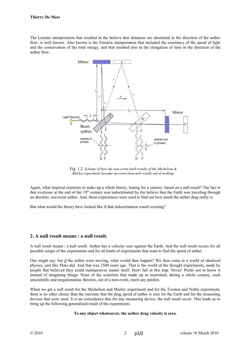
The Lorentz interpretation that resulted in the believe that distances are shortened in the direction of the aether flow, is well known. Also known is the Einstein interpretation that included the constancy of the speed of light and the conservation of the total energy, and that resulted also in the elongation of time in the direction of the aether flow.
Fig. 1.2. Scheme of how the non-event (null-result) of the Michelson & Morley experiment became an event (non-null result) out of nothing.
Again, what inspired scientists to make up a whole theory, lasting for a century, based on a null result? The fact is that everyone at the end of the 19th century was indoctrinated by the believe that the Earth was traveling through an absolute, universal aether. And, those experiences were used to find out how much the aether drag really is.
But what would the theory have looked like if that indoctrination wasn't existing?
2. A null result means : a null result.
A null result means : a null result. Aether has a velocity zero against the Earth. And the null result occurs for all possible setups of the experiments and for all kinds of experiments that want to find the speed of aether.
One might say: but if the aether were moving, what would then happen? We then come in a world of idealized physics, just like Plato did. And that was 2500 years ago. That is the world of the thought experiments, made by people that believed they could outmaneuver nature itself. Don't fall in this trap. Never! Prefer not to know it instead of imagining things. None of the scientists that made up or nourished, during a whole century, such unscientific and megalomaniac theories, out of a non-event, merit any pardon.
When we get a null result for the Michelson and Morley experiment and for the Trouton and Noble experiment, there is no other choice than the outcome that the drag speed of aether is zero for the Earth and for the measuring devices that were used. It is no coincidence that for any measuring device, the null result occur. This leads us to bring up the following generalized result of the experiments.
To any object whatsoever, the aether drag velocity is zero.
© 2010 release 18 March 20102
Mirror
Mirror
Beam splitter
p10

Thierry De Mees
Since the speed of light is always measured as being c , this makes sense. I mean that if the aether's drag velocity is always measured as being zero, the velocity of light should also be measured as being c .We can even say that the speed of light is always c if we compare it to 'its proper' aether. That is, whatever the speeds of several object are, the speed of light will always be c for each of the objects! Thus: consequence one:
The speed of light in its aether is always c.
Isn't this the same as what Einstein said? Not quite. We see that the consequence of the assumption is that aether is not an absolute, universal aether, as was believed at the end of the 19 th century, but a local, mass-bounded aether. Because for any body, the aether speed is zero and the speed of light is c .
The only possible outcome to make these issues fit, is to account for a fluid-like aether. The latter guarantees that light will always travel at the same speed c against 'its own' aether, and only be refracted when passing from one to another zone of the aether, where theoretically slightly different densities may occur. This refraction guarantees also that there will not be any loss of light. Reflection is not an option for light through aether with slightly changing densities. Only strongly differing media allow for reflection. Thus, consequence two:
Aether behaves like fluid dynamics.
How exactly does aether behave and what are the consequences for light? This has to be investigated by setting up experiments. But the main issue for such experiments is the presence of the aether of the Earth, which will overwhelm the other aethers. One of the most discussed items in the past was the description of the transformation between relative systems, the simultaneity of events and the twin paradox. These items again are false issues, because they are created from thought experiments, based on a null-result experiment.And if one says: “but if we want to know simultaneity, how to manage that?”, we have to get back to gravitomagnetism, that solved so many cosmic issues up to now.(see: http://wbabin.net/papers.htm#De%20Mees).
The first things to realize then is that (see my papers “Did Einstein cheat?” and “On the Origin of the Lifetime Dilation of High Velocity Mesons”):
1. there is no proven mass increase due to velocity. Instead, a gravitation field increase occurs.2. there is no proven time dilatation due to velocity. Instead, a cylindrical compression occurs; clock systems can be delayed differently, depending from their mechanism.3. there is no proven length contraction due to velocity. However, a certain length contraction is expected by gravitomagnetism.
One issue however cannot directly be solved by gravitomagnetism : the fluid dynamics of aether. It should be associated to cosmological reasoning and to experiments.
3. Conclusion.
When analyzing the non-event of the Michelson & Morley and the Trouton & Noble experiments, it is clear that 1°: to any object whatsoever, the aether drag velocity is zero, 2°: the speed of light in its aether is always c, and 3°: aether behaves like fluid dynamics. The astonishing change of these non-events (null-results) into events (non-null results) by scientists is unworthy and made themselves irresponsible. It also persevered the wrong idea of a universal global aether drag. The mislead became even more underhand in SRT by denying the need of an aether.
© 2010 release 18 March 20103 p11

Thierry De Mees
4. References and interesting literature.
1. De Mees, T., 2003, A coherent double vector field theory for Gravitation.
2. De Mees, T., 2004, Did Einstein cheat ?
3. Feynman, Leighton, Sands, 1963, Feynman Lectures on Physics Vol 2.
4. Heaviside, O., A gravitational and electromagnetic Analogy, Part I, The Electrician, 31, 281-282 (1893)
5. Jefimenko, O., 1991, Causality, Electromagnetic Induction, and Gravitation, (Electret Scientific, 2000).
6. De Mees, T., 2003-2010, list of papers : http://wbabin.net/papers.htm#De%20Mees
© 2010 release 18 March 20104 p12

© 2003 Thierry De Mees
A coherent dual vector field theory for gravitationAnalytical method – Applications on cosmic phenomena
T. De Mees - [email protected]
Abstract
This publication concerns the fundamentals of the dynamics of masses interacting by gravitation. We start with the Maxwell analogy for gravitation or the Heaviside field, and we develop a model. This model ofdynamics, which we know takes in account the retardation of light, allow us to quantify the transfer of angularmovement point by point by the means of vectors, and to bring a simple, precise and detailed explanation to a largenumber of cosmic phenomena. And to all appearances, the theory completes gravitation into a wave theory.
With this model the flatness of our solar system and our Milky way can be explained as being caused by an angularcollapse of the orbits, creating so a density increase of the disc. Also the halo is explained. The “missing mass” (darkmatter) problem is solved, and without harming the Keplerian motion law. The theory also explains the deviation of mass like in the Diabolo shape of rotary supernova having mass losses, and itdefines the angle of mass losses at 0° and at 35°16’.Some quantitative calculations describe in detail the relativistic attraction forces maintaining entire the fast rotatingstars, the tendency of distortion toward a toroid-like shape, and the description of the attraction fields outside of a rotaryblack hole. Qualitative considerations on the binary pulsars show the process of cannibalization, with the repulsion ofthe mass at the poles and to the equator, and this could also explain the origin of the spin-up and the spin-down process.The bursts of collapsing rotary stars are explained as well. The conditions for the repulsion of masses are alsoexplained, caused by important velocity differences between masses. Orbit chaos is better explained as well. Finally,the demonstration is made that gyrotation is related to the Relativity Theory.
Keywords. gravitation – star: rotary – disc galaxy – repulsion – relativity – gyrotation – gravitomagnetism – chaosMethods : analyticalPhotographs : ESA / NASA
Index
1. Introduction : the Maxwell analogy for gravitation: a short history. / Lecture A : a word on the Maxwell analogy.
2. Law of gravitational motion transfer. / Lecture B : a word on the flux theory approach.Lecture C : a word on the application of the Stokes theorem and on loop integrals.
3. Gyrotation of a moving mass in an external gravitational field.
4. Gyrotation of rotating bodies in a gravitational field.
5. Angular collapse into prograde orbits. Precession of orbital spinning objects. / The angular collapse of orbits intoprograde equatorial orbits / The precession of orbital spinning objects / Lecture D : a word on planetary systems.
6. Structure and formation of prograde disc Galaxies. / Objects with an orbit / Objects without an orbit / Stellarclusters’ trajectories / Calculation of the constant velocity of the stars around the bulge of plane galaxies /Example : calculation of the stars’ velocity of the Milky Way / Dark matter and missing mass are not viable /Lecture E : a word on the formation of disc galaxies.
7. Unlimited maximum spin velocity of compact stars.
8. Origin of the shape of mass losses in supernovae.
9. Dynamo motion of the sun.
10. Binary stars with accretion disc. / Fast rotating star analysis : creation of bursts, turbulent accretion disks / Burstsof collapsing stars / Calculation method for the accretion disc of a binary pulsar.
11. Repulsion by moving masses.
12. Chaos explained by gyrotation.
13. The link between Relativity Theory and Gyrotation Theory.
14. Discussion : implications of the relationship between Relativity and Gyrotation / Paper: Relativity theory analysed.
15. Conclusion
16. References
1 p13
© 2003 Thierry De Mees
1. Introduction : the Maxwell analogy for gravitation: a short history.
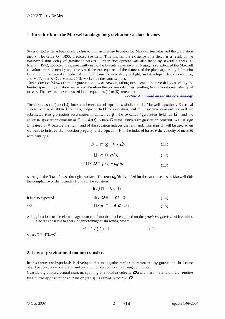
Several studies have been made earlier to find an analogy between the Maxwell formulas and the gravitationtheory. Heaviside O., 1893, predicted the field. This implies the existence of a field, as a result of thetransversal time delay of gravitation waves. Further development was also made by several authors. L.Nielsen, 1972, deducted it independently using the Lorentz invariance. E. Negut, 1990 extended the Maxwellequations more generally and discovered the consequence of the flatness of the planetary orbits, JefimenkoO., 2000, rediscovered it, deducted the field from the time delay of light, and developed thoughts about it,and M. Tajmar & C.de Matos, 2003, worked on the same subject. This deduction follows from the gravitation law of Newton, taking into account the time delay caused by thelimited speed of gravitation waves and therefore the transversal forces resulting from the relative velocity ofmasses. The laws can be expressed in the equations (1) to (5) hereunder.
Lecture A : a word on the Maxwell analogy
The formulas (1.1) to (1.5) form a coherent set of equations, similar to the Maxwell equations. Electricalcharge is then substituted by mass, magnetic field by gyrotation, and the respective constants as well are
substituted (the gravitation acceleration is written as g , the so-called “gyrotation field” as Ω Ω Ω Ω , and the
universal gravitation constant as G-1 = 4π ζ , where G is the “universal” gravitation constant. We use sign⇐ instead of = because the right hand of the equation induces the left hand. This sign ⇐ will be used whenwe want to insist on the induction property in the equation. F is the induced force, v the velocity of mass mwith density ρ.
F ⇐ m (g + v × ΩΩΩΩ) (1.1)
∇∇∇∇ . g ⇐ ρ / ζ (1.2)
(1.3)
where j is the flow of mass through a surface. The term ∂g/∂t is added for the same reasons as Maxwell did:the compliance of the formula (1.3) with the equation
It is also expected div ΩΩΩΩ ≡ ∇ ∇ ∇ ∇. ΩΩΩΩ = 0 (1.4)
and ∇∇∇∇× g ⇐ - ∂ ΩΩΩΩ / ∂ t (1.5)
All applications of the electromagnetism can from then on be applied on the gravitomagnetism with caution.Also it is possible to speak of gravitomagnetism waves, where
c2 = 1 / ( ζ τ ) (1.6)
where τ = 4πG/c2.
2. Law of gravitational motion transfer.
In this theory the hypothesis is developed that the angular motion is transmitted by gravitation. In fact noobject in space moves straight, and each motion can be seen as an angular motion.
Considering a rotary central mass m1 spinning at a rotation velocity ωωωω and a mass m2 in orbit, the rotation
transmitted by gravitation (dimension [rad/s]) is named gyrotation ΩΩΩΩ.
© Oct. 2003 update 1/09/2004
div j ⇐ - ∂ρ / ∂ t
c² ∇∇∇∇× ΩΩΩΩ ⇐ j / ζ + ∂g /∂ t
2 p14

© 2003 Thierry De Mees
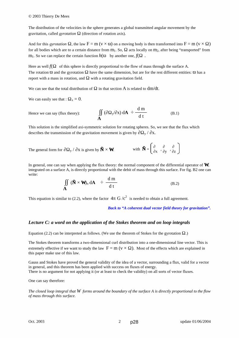
Equation (1.3) can also be written in the integral form as in (2.1), and interpreted as a flux theory. It
expresses that the normal component of the rotation of Ω Ω Ω Ω , integrated on a surface A, is directly proportionalwith the flow of mass through this surface.
For a spinning sphere, the vector ΩΩΩΩ is solely present in one direction, and ∇∇∇∇ × ΩΩΩΩ expresses the distribution
of ΩΩΩΩ on the surface A. Hence, one can write:
(2.1)
Lecture B : a word on the flux theory approach
In order to interpret this equation in a convenient way, the theorem of Stokes is used and applied to the
gyrotation ΩΩΩΩ . This theorem says that the loop integral of a vector equals the normal component of thedifferential operator of this vector.
Lecture C : a word on the application of the Stokes theorem and on loop integrals
(2.2)
Hence, the transfer law of gravitation rotation (gyrotation) results in:
(2.3)
This means that the movement of an object through another gravitation field causes a second field, calledgyrotation. In other words, the (large) symmetric gravitation field can be disturbed by a (small) movingsymmetric gravitation field, resulting in the polarisation of the symmetric transversal gravitation field into anasymmetric field, called gyrotation (analogy to magnetism). The gyrotation works perpendicularly onto othermoving masses. By this, the polarised (= gyrotation) field expresses that the gravitation field is partly madeof a force field, which is perpendicular to the gravitation force field, but which annihilate itself if nopolarisation has been induced.
3. Gyrotation of a moving mass in an external gravitational field.
It is known from the analogy with magnetism that a moving mass in a gravitation reference frame will causea circular gyrotation field (fig. 3.1). Another mass which moves in this gyrotation field will be deviated by aforce, and this force works also the other way around, as shown in fig. 3.2.
The gyrotation field, caused by the motion of m is given by (3.1) using (2.3). The equipotentials are circles:
(3.1)
Perhaps the direction of the gravitation field is important. With electromagnetism in a wire, the direction ofthe (large) electric field is automatically the drawn one in fig 3.1., perpendicularly to the velocity of theelectrons.
fig. 3.1 fig. 3.2
© Oct. 2003 update 1/09/2004
∫ ΩΩΩΩ . dl = ∫∫ (∇∇∇∇ × ΩΩΩΩ)n dA
A
∫∫ (∇∇∇∇ × ΩΩΩΩ)n dA ⇐ 4π G m /c2
A
.
∫ ΩΩΩΩ .dl ⇐ 4π G m / c2.
ΩΩΩΩ m
g
. ΩΩΩΩ ΩΩΩΩm m F F g
..
2π R.Ωp ⇐ 4π G m / c2.
3 p15

z fig. 4.1 p r
m α y
ax R
© 2003 Thierry De Mees
In this example, it is very clear how (absolute local) velocity has to be defined. It is compared with the steadygravitation field where the mass flow lays in.This application can also be extrapolated in the example below: the gyrotation of a rotating sphere.
4. Gyrotation of rotating bodies in a gravitational field.
Consider a rotating body like a sphere. We will calculate the gyrotation at acertain distance from it, and inside. We consider the sphere being envelopedby a gravitation field, generated by the sphere itself, and at this condition,we can apply the analogy with the electric current in closed loop.
The approach for this calculation is similar to the one of the magnetic fieldgenerated by a magnetic dipole.
Each magnetic dipole, created by a closed loop of an infinitesimal rotatingmass flow is integrated to the whole sphere. (Reference: Richard Feynmann: Lectures on Physics)
The results are given by equations inside the sphere and outside the sphere:
Fig. 4.2
(4.1)
(4.2)
(Reference: Eugen Negut, www.freephysics.org) The drawing shows equipotentials of – Ω .
For homogeny rigid masses we can write :
(4.3)
When we use this way of thinking, we should keep in mind that the sphere is supposed to be immersed in asteady reference gravitation field, namely the gravitation field of the sphere itself .
5. Angular collapse into prograde orbits. Precession of orbital spinning objects.
Concerning the orbits of masses, when the central mass (the sun) rotates, there are found two major effects.
The angular collapse of orbits into prograde equatorial orbits.In analogy with magnetism, it seems acceptable that the field lines of the gyrotation ΩΩΩΩ, for the space outsideof the mass itself, have equipotential lines as shown in fig. 5.1. For every point of the space, a localgyrotation can be found.
© Oct. 2003 update 1/09/2004
Y p
r X
R
Ωint ⇐ −FHG
IKJ −
•LNM
OQP
4 2
5
1
3 52 2π ρ ω
ωG
c2 r Rr rb g
Ωext 3 2
G
5 c⇐ −
•FHG
IKJ
4
3 5
5π ρ ω ωRr
r rb g
Ωext 3 2 2
G
5 c⇐ −
•FHG
IKJ
m Rr
r r
r
2 3ω
ωb g
4 p16
© 2003 Thierry De Mees
Fig. 5.1
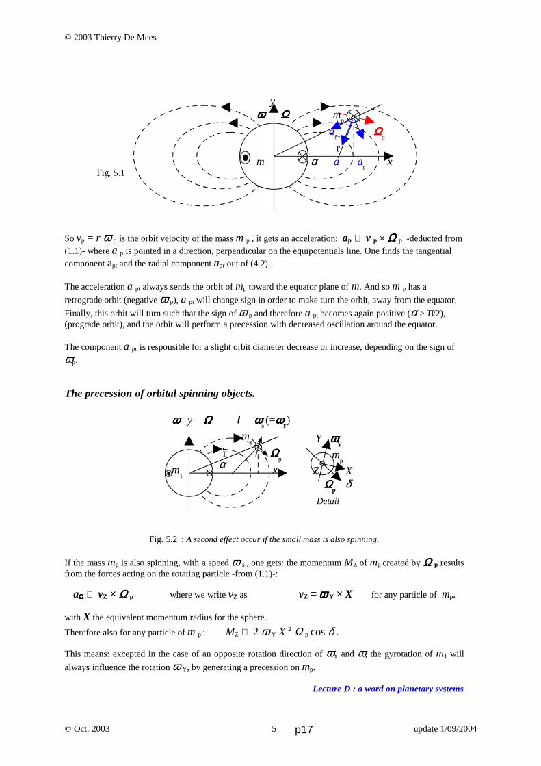
So vp = r ω p is the orbit velocity of the mass m p , it gets an acceleration: ap ⇐ v p × Ω Ω Ω Ω p -deducted from(1.1)- where a p is pointed in a direction, perpendicular on the equipotentials line. One finds the tangentialcomponent apt and the radial component apr out of (4.2).
The acceleration a pt always sends the orbit of mp toward the equator plane of m. And so m p has a
retrograde orbit (negative ω p), a pt will change sign in order to make turn the orbit, away from the equator.
Finally, this orbit will turn such that the sign of ω p and therefore a pt becomes again positive (α > π/2),(prograde orbit), and the orbit will perform a precession with decreased oscillation around the equator.
The component a pr is responsible for a slight orbit diameter decrease or increase, depending on the sign of
ωp.
The precession of orbital spinning objects.
Fig. 5.2 : A second effect occur if the small mass is also spinning.
If the mass mp is also spinning, with a speed ω s , one gets: the momentum MZ of mp created by Ω Ω Ω Ω p resultsfrom the forces acting on the rotating particle -from (1.1)-:
aΩΩΩΩ ⇐ vZ × Ω Ω Ω Ω p where we write vZ as vZ = ω ω ω ω Y × X for any particle of mp.
with X the equivalent momentum radius for the sphere.
Therefore also for any particle of m p : MZ ⇐ 2 ω Y X 2 Ω p cos δ .
This means: excepted in the case of an opposite rotation direction of ωY and ω, the gyrotation of m1 will
always influence the rotation ω Y, by generating a precession on mp.
Lecture D : a word on planetary systems
© Oct. 2003 update 1/09/2004
y ωωωω ΩΩΩΩ m
p
ar
ΩΩΩΩp
rm α a a
tx
Y ωωωωY
mp
Z X ΩΩΩΩ
p δ
ω ω ω ω y ΩΩΩΩ l ωωωωs (=ωωωω
Y)
mp
r ΩΩΩΩp
m1
x
α
Detail
5 p17
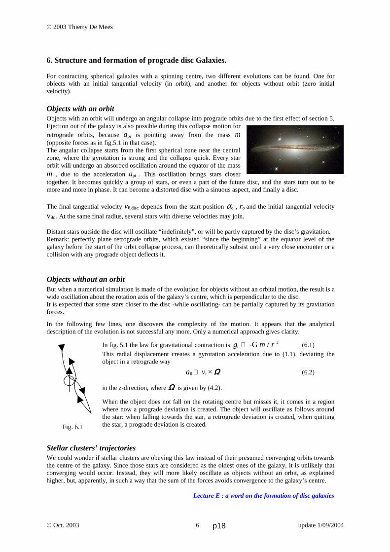
Fig. 6.1
© 2003 Thierry De Mees
6. Structure and formation of prograde disc Galaxies.
For contracting spherical galaxies with a spinning centre, two different evolutions can be found. One forobjects with an initial tangential velocity (in orbit), and another for objects without orbit (zero initialvelocity).
Objects with an orbitObjects with an orbit will undergo an angular collapse into prograde orbits due to the first effect of section 5.Ejection out of the galaxy is also possible during this collapse motion forretrograde orbits, because apr is pointing away from the mass m(opposite forces as in fig.5.1 in that case).The angular collapse starts from the first spherical zone near the centralzone, where the gyrotation is strong and the collapse quick. Every starorbit will undergo an absorbed oscillation around the equator of the massm , due to the acceleration apt . This oscillation brings stars closertogether. It becomes quickly a group of stars, or even a part of the future disc, and the stars turn out to bemore and more in phase. It can become a distorted disc with a sinuous aspect, and finally a disc.
The final tangential velocity vθ,disc depends from the start position αo , ro and the initial tangential velocity
vθο. At the same final radius, several stars with diverse velocities may join.
Distant stars outside the disc will oscillate “indefinitely”, or will be partly captured by the disc’s gravitation. Remark: perfectly plane retrograde orbits, which existed “since the beginning” at the equator level of thegalaxy before the start of the orbit collapse process, can theoretically subsist until a very close encounter or acollision with any prograde object deflects it.
Objects without an orbitBut when a numerical simulation is made of the evolution for objects without an orbital motion, the result is awide oscillation about the rotation axis of the galaxy’s centre, which is perpendicular to the disc. It is expected that some stars closer to the disc -while oscillating- can be partially captured by its gravitationforces.
In the following few lines, one discovers the complexity of the motion. It appears that the analyticaldescription of the evolution is not successful any more. Only a numerical approach gives clarity.
In fig. 5.1 the law for gravitational contraction is gr ⇐ -G m / r 2 (6.1)
This radial displacement creates a gyrotation acceleration due to (1.1), deviating theobject in a retrograde way
aθ ⇐ vr × ΩΩΩΩ (6.2)
in the z-direction, where ΩΩΩΩ is given by (4.2).
When the object does not fall on the rotating centre but misses it, it comes in a regionwhere now a prograde deviation is created. The object will oscillate as follows aroundthe star: when falling towards the star, a retrograde deviation is created, when quittingthe star, a prograde deviation is created.
Stellar clusters’ trajectoriesWe could wonder if stellar clusters are obeying this law instead of their presumed converging orbits towardsthe centre of the galaxy. Since those stars are considered as the oldest ones of the galaxy, it is unlikely thatconverging would occur. Instead, they will more likely oscillate as objects without an orbit, as explainedhigher, but, apparently, in such a way that the sum of the forces avoids convergence to the galaxy’s centre.
Lecture E : a word on the formation of disc galaxies
© Oct. 2003 update 1/09/20046 p18

© 2003 Thierry De Mees
Calculation of the constant velocity of the stars around the bulge of plane galaxiesLet's take the spherical galaxy again with a rotary centre (fig. 6.2). The distribution of the mass is such, that astar only feels the gravitation of the centre. We consider equal masses Mo (mass of the centre, named “the
bulge”) in various concentric hollow spheres according to some function of R(it must not be linear). We take the total bulge as the centre mass because thatpart does not collapse into a disk, and so, it has to be considered as part of therotary centre of the galaxy. Possibly, the orbit can be disturbed by thepassage of other stars, but in general one can say that only the centre Mo hasan influence according to:
and (6.3) (6.4)
fig. 6.2 So, (6.5)
When the angular collapse of the stars is done, creating a disc around the bulge, the following effect occurs:
the mass which before took the volume (4/3) π R³, will now be
compressed in a volume π R² h where h is the height of the disc,that is a fraction of the diameter of the initial sphere (fig. 6.3).
And at the distance R, a star feels more gravitation than the onegenerated by the mass Mo.
To a distance k.Ro the star will be submitted to the influence ofabout n.Mo , where k and n are supposed to be linear functions passing through zero in the centre of thebulge.
Strong simplified, this gives for the total mass according to the distance R:
(6.6)
Therefore, one can conclude that :
Concerning the centre, zone zero, one cannot say much. Let's not forget that a part of the angular momentumhas been transmitted to the disc, and that the centre is not a point but a zone. For zone one, we can say that the function of the forces of gravitomagnetism must be somewhere betweenthe one of the initial sphere and the zone 2.
Example : calculation of the stars’ velocity of the Milky WayThese findings are completely compatible with themeasured values. The diagram shows a typical example, which shows thevelocities of stars for our Milky Way.
Using equation (6.6) for our Milky Way, with thereasonable estimate of a bulge diameter of 10000 lightyears having a mass of 20 billion of solar masses (10%of the total galaxy), and admitting that k = n we get aquite correct orbital velocity of 240 km/s (fig. 6.4).
© Oct. 2003 update 1/09/2004
m
Mo
Mo
Mo
Mo
vr2 = constant
250 km/s
0 5 kpc Rfig. 6.4
MoM
oM
o
h 1 0 1 2
fig. 6.3
F GM mRR = 0
2F
mvRC
R=2
F F vG MRR C R= ⇒ =2 0
vG nMk Rr2
2 0=
7 p19

© 2003 Thierry De Mees
Dark matter and missing mass are not viableThe problem of the 'missing mass' or ‘dark matter’ that have never beenfound and that had to bring an explanation for the stars’ velocityconstancy is better solved with our theory: the velocity constancy isentirely due to the formation of the plane galaxy without a need ofinvisible masses.
7. Unlimited maximum spin velocity of compact stars.
When a supernova explodes, this happens partially and in specific zones. The purpose here is to find out whythis happens so. Let us consider the fast rotary star, on which the forces on p are calculated (fig. 7.1). We don’t want topolemic on the correct shape for the supernova, and suppose that it is still a homogeny sphere. If the massdistribution is different, we will approximate it by a sphere.For each point p, the gyrotation can be found by putting r = R in (4.2). And taken in account the velocity ofp in this field, the point p will undergo a gyrotation force which is pointing towards the centre of the sphere.
Replacing also the mass by m = πR3ρ 4/3 we get (4.2) transformed as follows:
(7.1)
The gyrotation accelerations are given by the following equations:
ax ⇐ x ω Ω Ω Ω Ω y = ω R cosα Ω Ω Ω Ωy and ay ⇐ x ω Ω Ω Ω Ω x = ω R cosα Ω Ω Ω Ω x
To calculate the gravitation at point p, the sphere can be seen as a point mass. Taking in account thecentrifugal force, the gyrotation and the gravitation, one can find the total acceleration :
(7.2)
(7.3)
The gyrotation term is therefore a supplementary compression force that will stop the neutron star from
exploding. For elevated values of ω 2, the last term of (7.2) is negligible, and will maintain below a critical
value of R a global compression, regardless of ω. This limit is given by the Critical Compression Radius:
or R = RCα < RC (1 – 3 sin2α ) (7.4)
where RC is the Equatorial Critical Compression Radius for Rotary Spheres :
RC = G m / 5 c2 (7.5)
RC is 1/10th of the Schwarzschild radius RS valid for non-rotary black holes ! This means that black holescan explode when they are fast spinning, and that every non-exploding spinning star must be a black hole.
© Oct. 2003 update 1/09/2004
Fig. 7.1
y ωωωω ΩΩΩΩ p
m α x
r R
ΩR 2 2
G
5 c⇐ −
•FHG
IKJ
mR
R R
Rω
ω3 b g
a RG m
RG m
Rx tot ⇐ −−F
HGIKJ
−ω αα α2
2
21
1 3cos
sin cosc h5 c2
− ⇐ + +aG m Gm
Ry tot 03 2 2
2
ω α α αcos sin sin
c2
0 11 3 2
= −−G m
R
sin αc h5 c2
8 p20

© 2003 Thierry De Mees
The fig. 7.2 shows the gyrotation and the centrifugal forces at the surface of a spherical star. The samededuction can be made for the lines of gyrotation inside the star. Fig. 7.3 shows the gyrotation lines andforces at the inner side of the star. We see immediately that (7.4) has to be corrected : at the equator, the
gyrotation forces of the inner and the outer material are opposite. So, (7.4) is valid for α ≠ 0.
From (7.4) also results that the shape of fast rotating stars stretches toward an Dyson ellipse and even atoroid:
if α ≥ 35°16’ the Critical Compression Radius becomes indeed zero. Contraction will indeed increase thespin and change the shape to a “tire” or toroid black hole, like some numeric calculations seem to indicate.(Ansorg et al., 2003, A&A, Astro-Ph.).
8. Origin of the shape of mass losses in supernovae.
When a rotary supernova ejects mass, the forces can bedescribed as in section 6 for objects without an orbit, butwith an high initial velocity from the surface of the star. Dueto (1.1) , at the equator the ejected mass is deviated in aprograde ring, which expansion slows down by gravitationand will in the end collapse when contraction starts again,but by maintaining the prograde rings as orbits.
When the mass leave under angle, a prograde ring isobtained, parallel to the equator, but outside of the equator’splane. This ring expands in a spiral, away from the star, because of its initial velocity. The expansion slowsdown, and will get an angular collapse by the gyrotation working on the prograde motion.
The probable origin of the anglehas been given in section 7: thezones of the sphere near thepoles (35°16’ to 144°44’ and-35°16’ to -144°44’) are the“weakest”. Indeed, these zoneshave a gyrotation pointingperpendicularly on the surface ofthe sphere, so that the gyrotationacceleration points tangentiallyat this surface, so that nocompensation with thecentripetal force is possible. Thezone near the equator (0°) has nogyrotation force which couldhold the mass together in compensation of the centripetal force.
The observation complies perfectly with this theoretical deduction. The supernovae explode into symmetriclobes, with a central disc. Observation will have to verify that these lobes start nearly at 35°, measured fromthe equator.
© Oct. 2003 update 1/09/2004
Fig. 7.2 Fig. 7.3
ΩΩΩΩ
ΩΩΩΩ y
x
Fig. 8.1
SN 1987A η Carinae
SN 1987A: a local mass loss took place on the equator and probably close to the 35° 16’ angle. The zone 35°16’ to 144°44’ exploded possibly much earlier, and became a toroid-like shaped rotary star.η Carinae : mass loss by complete shells, probably above the 35° 16’ angle, forming two lobes with a central ring.
9 p21
© 2003 Thierry De Mees
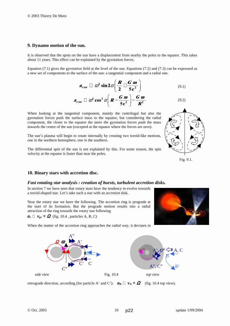
9. Dynamo motion of the sun.
It is observed that the spots on the sun have a displacement from nearby the poles to the equator. This takesabout 11 years. This effect can be explained by the gyrotation forces.
Equation (7.1) gives the gyrotation field at the level of the sun. Equations (7.2) and (7.3) can be expressed asa new set of components to the surface of the sun: a tangential component and a radial one.
(9.1)
(9.2)
When looking at the tangential component, mainly the centrifugal but also thegyrotation forces push the surface mass to the equator, but considering the radialcomponent, the closer to the equator the more the gyrotation forces push the massinwards the centre of the sun (excepted at the equator where the forces are zero).
The sun’s plasma will begin to rotate internally by creating two toroid-like motions,one in the northern hemisphere, one in the southern.
The differential spin of the sun is not explained by this. For some reason, the spinvelocity at the equator is faster than near the poles.
10. Binary stars with accretion disc.
Fast rotating star analysis : creation of bursts, turbulent accretion disks.In section 7 we have seen that rotary stars have the tendency to evolve towardsa toroid-shaped star. Let’s take such a star with an accretion disk.
Near the rotary star we have the following. The accretion ring is prograde atthe start of its formation. But the prograde motion results into a radialattraction of the ring towards the rotary star following
ar ⇐ vpr × ΩΩΩΩ (fig. 10.4 , particles A, B, C)
When the matter of the accretion ring approaches the radial way, it deviates in
retrograde direction, according (for particle A’ and C’): aR ⇐ vA × ΩΩΩΩ (fig. 10.4 top view).
© Oct. 2003 update 1/09/2004
Fig. 9.1.
A’” A’, C’ A, C B
A”, C” B’
side view Fig. 10.4 top view
A”ΩΩΩΩ ωωωω A’
A B
C’ C
C”
aR G m
t tot ⇐ +FHG
IKJω α2 2
2sin
5c2
a RG m G m
Rr tot ⇐ −FHG
IKJ −ω α2 2
2cos5c2
10 p22

© 2003 Thierry De Mees
With fast rotating heavy masses this acceleration is enormous. Then, when the particles go by retrograde way,
again an acceleration is exerted on the particles in another direction aP ⇐ vR × ΩΩΩΩ (particles A”, C”). As a consequence these particles are projected away from the poles. At the level of the equator, the mass is sent back towards the accretion disc (particles B, B’). We expect anaccretion ring whose closest fraction to the rotary star is almost standing still, with local prograde vortices.
If a particle, due to collisions, gets inside the toroid to the level of the equator, it can be trapped by the gyrotationin a retrograde orbit (particle A”’), or if prograde, absorbed. This effect can result in a temporary crowding, afterwhich the accumulation should disappear again due to the limited space and because of the local gyrotationforces. The observed spin-up and spin-down effects are possibly explained by these trapped particles.
When these phenomena are observed, high energy X-rays are related to it. It seems not likely that these X-rayswould be gravitational waves. But there is another possible origin for these X-rays. One should not forget thatthe velocity of the bursts is extremely high, and probably faster than light for some particles. Both the relativitytheory and the ether theories would say that high energies are involved. Considering that matter is “trappedlight”, and for ether theories, that the particles are forced through a slow ether, the stability of these particlescould be harmed seriously. If so, the light can escape from the trap, and scatter as X-rays.
Bursts of collapsing stars.When a rotating star collapses, this happens in a very short time,and it will result in a burst. What is its process ?
The conservation of momentum causes a quick increase of its spinwhen a collapse occurs. And an increase of spin velocity results inan fast increase of gyrotation forces :
The law (1.5) : ∇ ∇ ∇ ∇ × g ⇐ - ∂ ΩΩΩΩ / ∂ t
is responsible for a huge circular gravitation force in the accretion ring. The attraction occurs in a circular wayinstead of a radial one.The consequence is a strong contraction of the accretion ring, resulting in shrinking, and so a sudden repulsion ofaccretion matter, away from the star at the equator and at the poles, as described in the former section. A burst occurs both at the poles and at the level of the accretion ring (see fig. 10.4 and fig. 10.5).
Calculation method for the accretion disc of a binary pulsar.Consider fig. 10.4 in order to analyse the absorption process. Matter is absorbed according to equation (10.1),
and will be attracted by gravitation and gyrotation forces near the rotary star. This matter goes prograde, andsome of it will flow over the poles, which is then ejected as beams. Some prograde matter at the equator levelcan be absorbed by the rotary star. But some matter can stay near the rotary star as a cloud, which is subject tothe gyrotation pressure forces. A disc around the rotary star is being created according to this gyrotation pressure.The density of the ring will increase, and will approach the rotary star. But because of the limited thickness ofthe ring and it’s increasing pressure, it will also spill toward the outside. The masses that are pulled from thecompanion will then knock the widened ring (fig. 10.6).
© Oct. 2003 11 update 1/09/2004
ω ⊗ Ω g. .
Fig. 10.5
Fig. 10.6 Fig. 10.7
Fg F
Ω
v
p23

© 2003 Thierry De Mees
The equilibrium equations can be produced again, this time for a ring of gasses. However, the velocity vector ofthe inner part of the disc near the rotary star determines whether the disc material will be absorbed or ejected.Prograde matter can be attracted, but retrograde and in-falling matter is repulsed.
11. Repulsion by moving masses.
Repulsion of masses is deducted from drawing 10.4 (particle B), but also directly from the theory: when twoflows of masses dm/dt move in the same way in the same direction, the respective fields attract each other. For
flows of masses having an opposite velocity, their respective gyrotation fields will be repulsive. It is clear thatthe velocity of the two mass flows should be seen in relation to another mass, in (local) rest, and large enough toget gyrotation energy created, as explained in section 3.
Spinning masses do the same.
Fig. 11.2
Here however, the spinning masses themselves create the reference gravitation field needed to get the gyrotationeffects produced.
12. Chaos explained by gyrotation.
The theory can explain what happens when two planets cross eachother. Gravitation and gyrotation give an noticeable effect of achaotic interference. Let’s assume that the orbit’s radius of the smallplanet is larger than the one of the large planet. When passing by, ashort but considerable attraction moves the small planet into asmaller orbit.
At the same time, gyrotation works via aO ⇐ vR × ΩΩΩΩ on the planetin the following way (fig. 12.1): the sun’s and the large planet’sgyrotation act on this radial velocity of the planet by slowing downit’s orbital velocity. The result is a slower orbital velocity in asmaller orbit, which is in disagreement with the natural law of gravitation fashioned orbits :
v = (GM/r)-1/2 (12.1)
Thus, in order to solve the conflict, nature sends the small planet away to a larger orbit. Again, gyrotation workson the radial velocity, this time by increasing the orbital velocity, which contradicts again (12.1). We come so toan oscillation, which can persist if the following passages of the large planet come in phase with the oscillation.
One could say that only gravitation could already explain chaotic orbits too. No, it is not: if no gyrotation wouldexist, the law (12.1) would send the planet back in it’s original orbit with a fast decreasing oscillation. Gyrotationreinforces and maintains the oscillation much more efficiently, and allows even screwing oscillations.
© Oct. 2003 12 update 1/09/2004
m1
m2
Fig. 12.1(The orbits are represented as ellipses)
ΩΩΩΩ ΩΩΩΩm m F F
.. ΩΩΩΩ ΩΩΩΩ
F m m F..
Fig. 11.1
p24

© 2003 Thierry De Mees
13. The link between Relativity Theory and Gyrotation Theory.
Two flows of masses m moving in the same way in the same direction, attract. Whether one observer follows themovement or not, the effect must remain the same when we apply the relativity principle.
The two points of view are compared hereunder.
Gyrotation Gravitation
Fig. 12.1
The following notations are used:
and m = dm/dlFor the gyrotation part, the work can be found from the basic formulas in sections 1 until 3 :
where F = dF/dl and τ = 4π G/c2.
So,
Hence, the work is :
F.dr = 2 G m2 v2/(r c2) dr (13.1)
For the gravitation part, the gravitation of m acting on dl is integrated, which gives :
F = 2 G m2 / r
The work is : F.dr = 2 G m2/r dr (13.2)
Let’s assume two observers look at the system in movement: an observer at (local) rest and one in movementwith velocity v. An observer at rest will say: the system in movement will exercise a work equal to the gravitation of the systemat rest, increased by the work exerted by the gyrotation of the system in motion. A moving observer will say: the system will exert a work equal to the gravitation (of the moving system). Because of the principle of relativity, the two observers are right. One can write therefore:
(13.3)
where “(mv)st” e.g. represents the moving mass, seen by the steady observer.We can assume (due to the relativity principle) that:
. Hence,
An important consequence of this is: the “relativistic effect” of gravitation, or better, the time delay of light isexpressed by gyrotation. This could be expected from the analogy with the electromagnetism.
© Oct. 2003 13 update 1/09/2004
d F dl m D m
α dl r
Ω d F
r m m
. .
m = dm/dt
.
.F ⇐ Ω m and 2π r.Ω ⇐ τ m
.
. .F = 2 G m2 /(r c2) . Now m = m.v
.
2 2 20
2 2 2G m
r
G m v
r
G m
rst st vst v
2
2
st
c
b g b g b g+ = +
m mst v v stb g b g= m m v cst st v st
b g b g= −1 2 2
p25
© 2003 Thierry De Mees
In other words: when the gravitation and the gyrotation are taken into account, the frame can be chosen freely,while guaranteeing a “relativistic” result.
The fact that the neutron stars don't explode can find its explanation through the forces of gyrotation, but canalso be seen as a “mass increase” due to the relativistic effect. The mass increase of the relativity theory ishowever an equivalent pseudo mass due to the gyrotation forces which act locally on every point.
14. Discussion : implications of the relationship between Relativity and Gyrotation.
The discussion about the paragraph 11 relates to the consequences for the relativity theory. This paragraph istreated separately in “Relativity theory analysed”, in order to not harm the objective of this paper which is toshow how the gyrotation works and what it offers for the study of the dynamics of objects.
Relativity theory analysed
15. Conclusions.
Gyrotation, defined as the transmitted angular movement by gravitation in motion, is a plausible solution for awhole set of unexplained problems of the universe. It forms a whole with gravitation, in the shape of a vectorfield wave theory, that becomes extremely simple by its close similarity to the electromagnetism. And in thisgyrotation, the time retardation of light is locked in. An advantage of the theory is also that it is Euclidian, and that predictions are deductible of laws analogous tothose of Maxwell.
16. References.
Adams, F., Laughlin, F., 1996, Astr-Ph., 9701131v1
Ansorg, M., Kleinwächter, A., Meinel, R., 2003, A&A 405, 711-721
Ansorg, M., Kleinwächter, A., Meinel, R., 2003, Astro-Ph., 482, L87
Alonso, M., Finn, E. J., 1973, Fundamental University Physics.
Caroll B. W., Ostlie, D. A., 1996, An Introduction to Modern Astrophysics.
Einstein, A., 1916, Über die spezielle und die allgemeine Relativitätstheorie.
Feynman, Leighton, Sands, 1963, Feynman Lectures on Physics Vol 2.
Negut, E., 1990, On intrinsic properties of relativistic motions.
Nielsen, L., 1972, Gamma No. 9, Niels Bohr Institute, Copenhagen
Tajmar, M. & de Matos, C.J., arXiv, 2003gr.qc.....4104D
Van Boekel, R., Kervella, P., Schöller, et al., 2003, A&A, 410, L37-L
Thanks go to Eugen Negut and Thomas Smid for their constructive remarks about the content.
© Oct. 2003 14 update 1/09/2004
p26

© 2003 Thierry De Mees
Oct. 2003 update 01/06/2004 1
Lectures on “A coherent dual vector field theory for gravitation”. The purpose of these lectures is to get more familiarized with gyrotation concepts and with its applications. Lecture A: a word on the Maxwell analogy Concerning our starting point, the Maxwell theory, it is known that the (induced) magnetic field of the electromagnetism is created by moving charges. We can even say, the only reason for the existence of the (induced) magnetic field is the velocity of charges, which are moving in a reference frame which has to be a field. We shall see later that the definition of item “velocity” is very important, and this will be approached in a different way than in the relativity theory, without harming nor contradicting the relativity theory. We know also that the magnetic field has an action which is perpendicular on the velocity vector of the charged particle, and that the Maxwell laws are complying with the Lorentz invariance, so it is “relativistic” and takes care of the time delay of light. The magnetic field has to be seen as a transversal interference (or the transversal distortion) of a moving charge’s electric field in a reference electric field. For an electric wire, this has been experienced. When the interference has been generated, this magnetic field will only influence other moving charges. It is attractive to say that also the gravitation is also influenced by moving masses, giving also a second field, which is analogue to the magnetism. And then, the Maxwell equations become very simple, because the charge is then replaced by the mass (Coulomb law to Newton law) and the gravito-magnetic field becomes the transmitted movement by gravitation, having the dimension s-1.
Back to “A coherent dual vector field theory for gravitation”. Lecture B: a word on the flux theory approach The basic induction formula of gyrotation can also be understood the following way: Imagine a rotating sphere with spin ω. We know from several observations (disk galaxies, planetary system) that the angular movement of the rotating centre is transmitted to the surrounding objects. So, what else but rotating gravitation field would transmit it? If we analyze m1 in the system of fig. B1, and if one can say that a certain effect is produced by gravitation in
motion, a certain function h(ω) , generated by the rotation of this mass m1, must be directly proportional to the flow dm1/dt. But we don't want to define the kinetic rotation of the rotary mass indeed, but the gyrotation to a certain distance of this rotary mass, generated by its gravitation field. Let’s show how this works.
Fig. B1 Let's take a spherical mass (in fact, the shape doesn't have any importance) that of course creates a field of gravitation, and that
spins with rotation velocity ω (see fig. B2). The study of an entity according to a flow can be made like a flux (of energy). To apply this theory, one can therefore define a surface A of the spinning mass in a stationary reference frame that will form half section of the sphere. We isolate the half circle A through which the whole mass of the sphere go in one cycle ("day"). A mass flow dm1/dt will move through this section.
ω m1 m2
ω Ω Α m1 y
x Fig. B2
p27
© 2003 Thierry De Mees
Oct. 2003 update 01/06/2004 2
The distribution of the velocities in the sphere generates a global transmitted angular movement by the
gravitation, called gyrotation Ω (direction of rotation axis). And for this gyrotation Ω, the law F = m (v × ω) on a moving body is then transformed into F = m (v × Ω)
for all bodies which are to a certain distance from m1. So, Ω acts locally on m2, after being “transported” from
m1. So we can replace the certain function h(ω) by another one, f(Ω). Here as well f(Ω) of this sphere is directly proportional to the flow of mass through the surface A.
The rotation ω and the gyrotation Ω have the same dimension, but are for the rest different entities: ω has a
report with a mass in rotation, and Ω with a rotating gravitation field. We can see that the total distribution of Ω in that section A is related to dm/dt. We can easily see that : Ωx = 0. Hence we can say (flux theory): (B.1) This solution is the simplified axi-symmetric solution for rotating spheres. So, we see that the flux which describes the transmission of the gravitation movement is given by ∂Ωy / ∂x. The general form for ∂Ωy / ∂x is given by ∇∇ × ΩΩ . In general, one can say when applying the flux theory: the normal component of the differential operator of ΩΩ , integrated on a surface A, is directly proportional with the debit of mass through this surface. For fig. B2 one can write:
(B.2) This equation is similar to (2.2), where the factor 4π G /c2 is needed to obtain a full agreement.
Back to “A coherent dual vector field theory for gravitation”. Lecture C: a word on the application of the Stokes theorem and on loop integrals
Equation (2.2) can be interpreted as follows. (We use the theorem of Stokes for the gyrotation Ω.) The Stokes theorem transforms a two-dimensional curl distribution into a one-dimensional line vector. This is extremely effective if we want to study the law F = m (v × Ω). Most of the effects which are explained in this paper make use of this law. Gauss and Stokes have proved the general validity of the idea of a vector, surrounding a flux, valid for a vector in general, and this theorem has been applied with success on fluxes of energy. There is no argument for not applying it (or at least to check the validity) on all sorts of vector fluxes. One can say therefore:
The closed loop integral that Ω forms around the boundary of the surface A is directly proportional to the flow of mass through this surface.
∫∫ (∇∇ × ΩΩ)n dA ÷ A
d m
d t
∫∫ (∂Ωy/∂x) dA ÷ A
d m
d t
with ∇∇ = , ,
∂ ∂ ∂ ∂x ∂y ∂z
p28
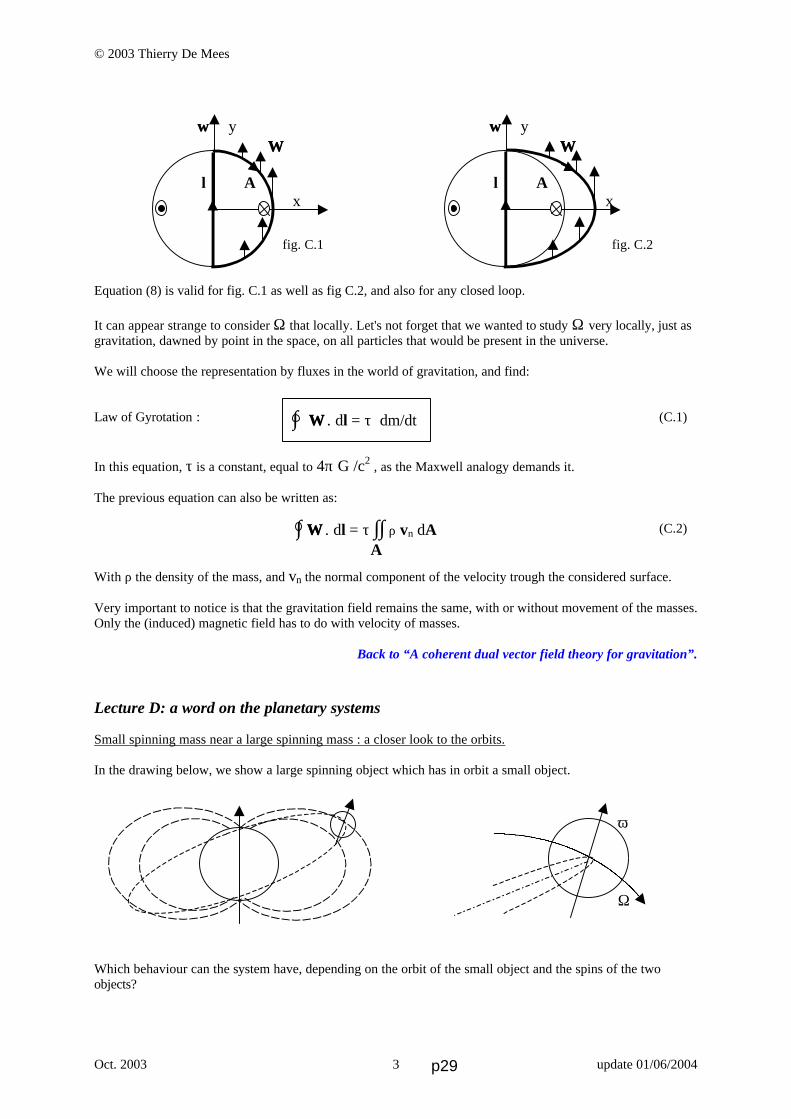
© 2003 Thierry De Mees
Oct. 2003 update 01/06/2004 3
fig. C.1 fig. C.2 Equation (8) is valid for fig. C.1 as well as fig C.2, and also for any closed loop.
It can appear strange to consider Ω that locally. Let's not forget that we wanted to study Ω very locally, just as gravitation, dawned by point in the space, on all particles that would be present in the universe. We will choose the representation by fluxes in the world of gravitation, and find: Law of Gyrotation : (C.1) In this equation, τ is a constant, equal to 4π G /c2 , as the Maxwell analogy demands it. The previous equation can also be written as:
(C.2) With ρ the density of the mass, and vn the normal component of the velocity trough the considered surface. Very important to notice is that the gravitation field remains the same, with or without movement of the masses. Only the (induced) magnetic field has to do with velocity of masses.
Back to “A coherent dual vector field theory for gravitation”. Lecture D: a word on the planetary systems Small spinning mass near a large spinning mass : a closer look to the orbits. In the drawing below, we show a large spinning object which has in orbit a small object. Which behaviour can the system have, depending on the orbit of the small object and the spins of the two objects?
ωω y ΩΩ l A x Α
ωω y ΩΩ l A x Α
∫ Ω Ω . dl = τ ∫∫ ρ vn dA A
∫ Ω Ω . dl = τ dm/dt
ω Ω
p29

© 2003 Thierry De Mees
Oct. 2003 update 01/06/2004 4
ω
Fc Ft Ω
F
The First Effect
The small mass, name it a planet, is rotating around a star. This is of course due to the gravitation force, in equilibrium with the centrifugal force. But in the gyrotation field of the star, the planet will feel another force, perpendicular to the gyrotation field. This force can be split in one force Fc pointing to the centre of the star, and one, Ft perpendicular to the first, tending to move the planet downwards. When the planet arrives after a half revolution at the other side, also the forces will be inverted:
Fc is still pointing to the centre of the star, and Ft tends this time to move the planet upwards. This will bring the planet away from the plane through the equator of the star. But when the orbit direction of the planet is retrograde (the orbit spin of the planet and the spin of star are opposite), the orbit derives away ! The star seems ejecting the planet ! What happens with this planet ? We check it out. The planet will move towards different oriented gyrotation fields of the star, but the orbit diameter will stay unchanged, as before. And after a while, it becomes a planet with an orbit in the other direction, in order to get forces which tend to the plane which is perpendicular to the spin of the star ! The first effect: In both cases, Fc will create a new equilibrium with the gravitation force, but Ft tend to move the planet in a plane, perpendicular to Ω. All the orbits of the planets tend to go in the same direction of the star’s spin, prograde. The Second Effect But what about the influence of the planet’s rotation? The planet can be seen as a multitude of rotating mass dipoles. Each dipole will feel the force F = m (v x Ω) and will create a momentum.
ω F
Ω
ω Ω
F
ω
Ω
F
Ω ω F
F
F Ω ω
F
F Ω ω
F F
ω Ω
ω F
Ω
ω F
Ω
ω
Ω
p30

© 2003 Thierry De Mees
Oct. 2003 update 01/06/2004 5
After a while, the planet arrives at the plane through the equator of the star. The direction of the forces change, but the momentum keeps the same direction. When the planet arrives at the other side of the orbit, the forces will turn differently again, as shown on the second drawing. Again, the same momentum as before is acting on the planet: it wants to put the rotation in the opposite direction than the direction of the spin of the star, as shown in the third drawing. We check this out with a few other situations: When the rotation axis is oriented in a different direction: And when the planet rotates in a plane perpendicular to the rotation axis of the star: We conclude that in this plane, the spin of the planet tends to put the its rotation parallel to the spin of the star, but in opposite direction. At the other hand, it is clear that in the two first examples, where the spin is almost parallel and in the same direction, the momentum tries to redress the rotation to an inversed spin, although it is a very small momentum compared with the momentum of the planet. The rotation becomes labile. Only the last drawing shown gives a stable situation.
Back to “A coherent dual vector field theory for gravitation”. Lecture E : a word on the formation of disk galaxies From a sphere to a disk. When we see at shapes of disk galaxies, how beautifully flat they are, it is strange that a rotating galaxy centre would be the reason of it. It is acceptable that the rotation of this centre is somehow transmitted to surrounding objects, but the flat shape is quite a surprise. However, the gyrotation forces explains perfectly this behaviour. The surrounding orbits obey to a downwards pressure if it is above the equator, and an upwards pressure if it is under the equator. Retrograde orbits are not allowed. Let’s follow the formation of such a galaxy. In order to fix ideas, we can imagine a small 'big bang' of a gigantic object permitting to give birth in a galaxy. We will follow the stars that remain in the action field of the system’s gravitation. The explosion is non symmetrical, causing the rotation of some parts. When the galaxy retract due to gravitation, the central zone can have a global angular momentum, whose spin velocity increases with its retraction. The phenomenon that we will describe starts at the centre of the galaxy: following the First Effect (see Lecture D), the orbit of every star orbit cannot be retrograde, but is prograde, and will move toward the equator plan the
ω F
F
Ω
ω
F F
Ω
F
F ω Ω
ω
F
F
Ω
p31
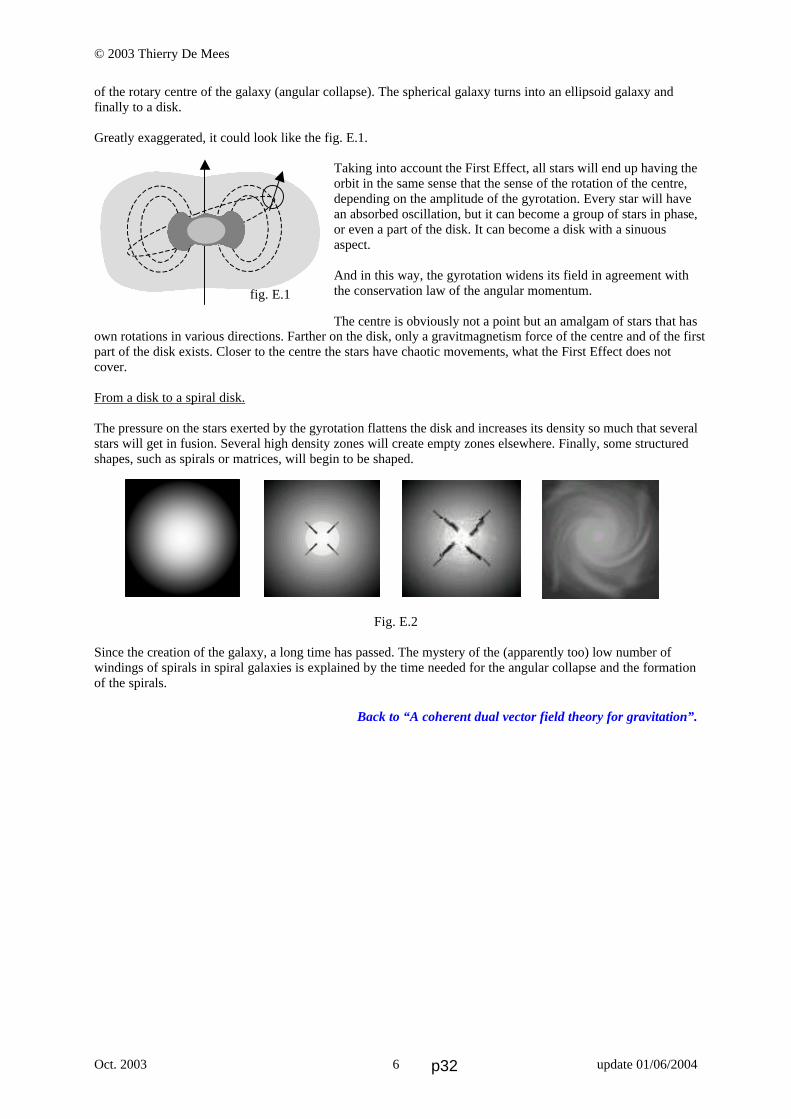
© 2003 Thierry De Mees
Oct. 2003 update 01/06/2004 6
of the rotary centre of the galaxy (angular collapse). The spherical galaxy turns into an ellipsoid galaxy and finally to a disk. Greatly exaggerated, it could look like the fig. E.1.
Taking into account the First Effect, all stars will end up having the orbit in the same sense that the sense of the rotation of the centre, depending on the amplitude of the gyrotation. Every star will have an absorbed oscillation, but it can become a group of stars in phase, or even a part of the disk. It can become a disk with a sinuous aspect. And in this way, the gyrotation widens its field in agreement with the conservation law of the angular momentum. The centre is obviously not a point but an amalgam of stars that has
own rotations in various directions. Farther on the disk, only a gravitmagnetism force of the centre and of the first part of the disk exists. Closer to the centre the stars have chaotic movements, what the First Effect does not cover. From a disk to a spiral disk. The pressure on the stars exerted by the gyrotation flattens the disk and increases its density so much that several stars will get in fusion. Several high density zones will create empty zones elsewhere. Finally, some structured shapes, such as spirals or matrices, will begin to be shaped.
Fig. E.2
Since the creation of the galaxy, a long time has passed. The mystery of the (apparently too) low number of windings of spirals in spiral galaxies is explained by the time needed for the angular collapse and the formation of the spirals.
Back to “A coherent dual vector field theory for gravitation”.
fig. E.1
p32
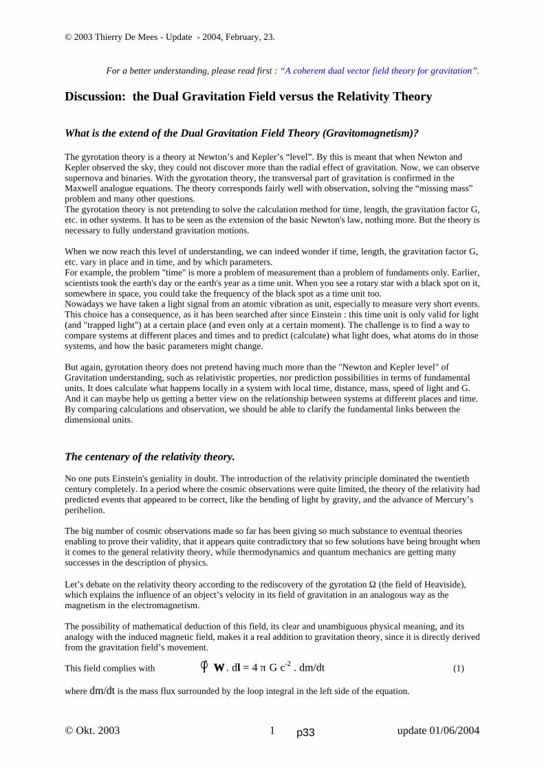
© 2003 Thierry De Mees - Update - 2004, February, 23.
© Okt. 2003 update 01/06/2004 1
For a better understanding, please read first : “A coherent dual vector field theory for gravitation”. Discussion: the Dual Gravitation Field versus the Relativity Theory What is the extend of the Dual Gravitation Field Theory (Gravitomagnetism)? The gyrotation theory is a theory at Newton’s and Kepler’s “level”. By this is meant that when Newton and Kepler observed the sky, they could not discover more than the radial effect of gravitation. Now, we can observe supernova and binaries. With the gyrotation theory, the transversal part of gravitation is confirmed in the Maxwell analogue equations. The theory corresponds fairly well with observation, solving the “missing mass” problem and many other questions. The gyrotation theory is not pretending to solve the calculation method for time, length, the gravitation factor G, etc. in other systems. It has to be seen as the extension of the basic Newton's law, nothing more. But the theory is necessary to fully understand gravitation motions. When we now reach this level of understanding, we can indeed wonder if time, length, the gravitation factor G, etc. vary in place and in time, and by which parameters. For example, the problem "time" is more a problem of measurement than a problem of fundaments only. Earlier, scientists took the earth's day or the earth's year as a time unit. When you see a rotary star with a black spot on it, somewhere in space, you could take the frequency of the black spot as a time unit too. Nowadays we have taken a light signal from an atomic vibration as unit, especially to measure very short events. This choice has a consequence, as it has been searched after since Einstein : this time unit is only valid for light (and "trapped light") at a certain place (and even only at a certain moment). The challenge is to find a way to compare systems at different places and times and to predict (calculate) what light does, what atoms do in those systems, and how the basic parameters might change. But again, gyrotation theory does not pretend having much more than the "Newton and Kepler level" of Gravitation understanding, such as relativistic properties, nor prediction possibilities in terms of fundamental units. It does calculate what happens locally in a system with local time, distance, mass, speed of light and G. And it can maybe help us getting a better view on the relationship between systems at different places and time. By comparing calculations and observation, we should be able to clarify the fundamental links between the dimensional units. The centenary of the relativity theory. No one puts Einstein's geniality in doubt. The introduction of the relativity principle dominated the twentieth century completely. In a period where the cosmic observations were quite limited, the theory of the relativity had predicted events that appeared to be correct, like the bending of light by gravity, and the advance of Mercury’s perihelion. The big number of cosmic observations made so far has been giving so much substance to eventual theories enabling to prove their validity, that it appears quite contradictory that so few solutions have being brought when it comes to the general relativity theory, while thermodynamics and quantum mechanics are getting many successes in the description of physics. Let’s debate on the relativity theory according to the rediscovery of the gyrotation Ω (the field of Heaviside), which explains the influence of an object’s velocity in its field of gravitation in an analogous way as the magnetism in the electromagnetism. The possibility of mathematical deduction of this field, its clear and unambiguous physical meaning, and its analogy with the induced magnetic field, makes it a real addition to gravitation theory, since it is directly derived from the gravitation field’s movement. This field complies with (1) where dm/dt is the mass flux surrounded by the loop integral in the left side of the equation.
∫ Ω Ω . dl = 4 π G c-2 . dm/dt
p33

© 2003 Thierry De Mees - Update - 2004, February, 23.
© Okt. 2003 update 01/06/2004 2
The Heaviside gyrotation field enables a precise description of many cosmic events, such as the formation of a plane galaxy, the shape of the supernova explosions, strengths keeping the fast rotating stars together, the torus shape of rotating black holes, etc. In the paper, “A coherent dual vector field theory for gravitation”, we examined two parallel mass fluxes with equal velocity in the same direction. One could conclude that the work of a moving system seen by an observer at rest equals W.(1+v²/c²), and the work of the moving system seen by a moving observer equals W. When we claimed the application of the equivalence principle we got the equation (2) The last term is zero because the velocity is zero in that case. Taking into account the relativity equivalence one could say that a mass at rest seen by a moving observer equals a moving mass seen by an observer at rest, (mst)v = (mv)st . This gives finally the requested equation (mst)st = (mv)st√(1-v2/c2). (3) When de gyrotation is taken into account, the factor √(1-v2/c2) is thus the difference between the gravitation of the moving system seen by a moving observer, and the gyrotation of the moving system seen by an observer at rest. To reduce the formula to one observer, one has only to apply the relativity principle (mst)v = (mv)st . But can one do such manoeuvres in physics with impunity? Lorentz’s transformation, Michelson-Morley’s experience, and Einstein’s relativity theory. Lorentz noticed an invariance on the Maxwell equations, by using the factor √(1-v2/c2). On the other hand, the experience of Michelson-Morley had to determine the speed of the ether, and theoretically foresaw the use of this same factor √(1-v2/c2) to this effect. It is therefore normal that this factor seemed essential to Einstein, which allowed him to prove the equation E = mc2 and on the other hand to postulate that the speed of light is constant in all directions (for the observer). The major advantage of the theory of relativity was that it did not necessitate to take into account the absolute speed of the ether. The experience of Michelson-Morley didn't succeed, which made of the invariance of Lorentz the ideal basis for a solution. This is what happened after the experience of Michelson-Morley : since it didn't result into anything, an inverse correction had to be made, resulting in the interference of the two light beams becoming zero after their separation and their re-grouping, as was required by the experience. It was in line with the assumption that the speed of light would be constant and identical in all directions. It legitimated the equation E = mc², which also necessitated the correction of the relativistic mass for all relative speeds (below c). The general relativity, which has as main actor the mass, forced Einstein to make a choice. Either to abandon the principle of relativity, because the masses fix the free movements in an absolute way (instead of a relative one), either to give to the invariance of Lorentz a “totalitarian” character: to consider the universe as deformed as gravitation "distorts" it, and to distort in precisely the same way the coordinates that describe this universe. Discussion of the experience of Michelson-Morley When at the test of Michelson-Morley the light is partially reflected and partially passed by the mirror, it is sent away by 90°. By the rotation of the earth a gyrotation force will work on the light, and bend it (depending from
2G(m2st)st 2G(m2
v)st v2 2G(m2
st)v r r c2 r + = + 0
p34
© 2003 Thierry De Mees - Update - 2004, February, 23.
© Okt. 2003 update 01/06/2004 3
the case, i.e. downwards). When the second mirror again reflects the light, the gyrotation works exactly in inverse direction (e.g. upwards). However, Michelson and Morley assumed that the light is sent in a certain direction, because of the moving ether, in order to get an interference (which corresponds to the contraction of Lorentz). If the ether of the earth has a speed zero, interference becomes indeed zero. Galaxies with a spinning centre. Earlier, we have studied disc galaxies. We have seen that the stars of galaxies balance either widely around the axis of rotation of the central black hole, either around its equator. It depends on the fact whether the star has an orbit or not. The orbit of the stars accelerates or slows down according to its change of slope, like a harmonic oscillator. A field that transmits the kinetic energy therefore exists: the gyrotation field. The speed must then be defined according to the strongest gravitation fields nearby, and in principle one gets for each object simultaneously a set of speeds, relative to each gravitomagnetism-field of the universe. If the strongest gravitomagnetism-fields nearby are taken away, the equation (2) seems to be correct, and to lead to Lorentz’ formula. Worlds In the special relativity theory, Einstein gave the example of two trains which move with a relative speed. Apart from those two trains nothing has been taken into account. Einstein created a "world". This means that the special relativity theory is only applicable for two trains with a relative movement, without any other object. When Einstein describes situations with a room falling freely in a gravitation field and with an accelerating room, Einstein again creates worlds. Nothing exists except this room and forces on that room. When one makes the equation (2), one has again created a world, because nothing existed outside the experience. But universe is not a lab. In reality we should always state that, i.e. for the left side or the right side of the equation (2) there exists a sufficiently large mass at finite distance, whose gravitation field reaches the test laboratory. Otherwise no “local absolute speed” can be defined. And only when no speed can be defined, we could make use of the relativity theory, and therefore get the equation (2) as a valid option. Experiment on ‘local absolute speed’ Consider the experience of parallel mass streams, but with opposite velocities (+v en –v). Depending on the immobile observer -compared to the mass streams-, or an observer moving with one of the streams, the results become totally different when using the gyrotation theory. But when one sees the observer as a large mass, the logic with the gyrotation theory comes back. But if we would do the experiment of chapter 12 in “A coherent dual vector field theory for gravitation” with mass streams at respective velocities –v and +v (placed at infinity from other masses), we may not replace those velocities by respectively 0 and 2v, because of the symmetry principle in nature. Theoretically, the results would be totally different when applying the theory blindly. Concerning the ether (the hypothetical carrier of light and gravitomagnetism waves), one has to acknowledge that it does not move in relation to the observer. Let’s leave unexplained if the ether is a separate entity, or if it is formed by a teamwork of the gravitomagnetism and the electromagnetism themselves. If one applies the gyrotation theory, one should state: the velocity of the ether (whatever it might be) is related to the sum of all the gravitomagnetism waves on the considered point. And its velocity is zero in relation to the object which measures its velocity. Only this way of seeing the ether is compatible with a constant speed of light. Thus, the velocity of an object must be seen in relation to all the existing gravitation and gyrotation fields on that object. Only then, a valid reference frame can be chosen, namely the strongest gravitation field(s) of the system.
p35

© 2003 Thierry De Mees - Update - 2004, February, 23.
© Okt. 2003 update 01/06/2004 4
Is the relativity theory wrong? When we limit its applications strictly to what is was meant originally, it is not wrong. The principles which are deducted from the retardation of light are of course valid. And when calculations are made for events that are related to light, this can lead to the Lorentz transformation as well. The relativity theory is applicable for light (electromagnetic waves) and gravitomagnetism waves. Perhaps even not for electromagnetic and gravitomagnetismfields. It describes accurately what a wave does according to the observer. It was seen earlier that the relativity theory applies the gyrotation, but that it is calculated backwards to the point of view of the observer. However there are many scientists who found imperfections to the theory of special relativity, or found improvements for three-dimensional applications. These researches will help astronomers interpreting observations. Indeed, the theory causes problems. When Einstein demonstrates the way how he calculates the relativity equation x2 - c2t2 = x’2- c2t’2 , he calculates the light motion in the +x direction and combines it with the light motion in the –x direction. He combines x – ct and x + ct into one equation, x2 - c2t2. How in physics can we combine two opposite motions at the same time? One plausible way is the following : a light beam which is subject to a transversal Doppler effect of its wave, whose wave-cycle goes first in the +x directions and than in the –x direction, resulting in x – ct and x + ct. But fundamental physics’ knowledge stops here. At the other hand, the relativity theory is not valid to explain how masses really behave. This explains the limited successes in this domain. All the successes of the relativity theory are exclusively related to how the observer sees the light, coming from an event somewhere in space. Is the relativity theory compatible with the gravitomagnetism theory? Yes, to a certain extend. Or better: they are both useful, but they describe different things. The relativity theory is only applicable in a restricted world, where the carrier of light is bounded with the observer, and without any fixed reference frame (such as it is valid for light). Moreover it only expresses how the data of light sources of a moving event can be mathematically transformed back for a stationary observer, but not what really happens with the objects. Indeed, if one assume that there is only gravitation (and not gyrotation) of a stationary observer towards the stationary frame, one must say (to apply the relativity theory): if one wants to have a moving frame examined by a stationary observer, one should do the following: look at the moving frame with a moving observer (thus simply the gravitation law) and adjust the point of view of the moving observer to the point of view of the stationary observer (deduction of the gyrotation law). Calculated the other way around (opposite to the gravitation + gyrotation laws) one can therefore express the moving frame (examined by a stationary observer) into a stationary frame which is corrected for its velocity. The application of the relativity theory did indeed arise the term of the gyrotation, but caught in an expression, just as if an observer would examine an egg and only see the shell, whereas in fact the yolk and the blank in the egg are present but hidden. And this happens really with light, because light adapts itself to each carrier of light, in other words, the ether of the masses where the light is coming through until the ether of the observer. This means that we have two valid approaches: one is the gravitomagnetism, valid for the description of dynamics, for any velocity, even faster than light, and another which is the relativity theory, only fully valid for the “perception” of electromagnetic and gravitomagnetism waves. Inertial mass and gravitational mass At the study of rapidly rotating stars we came at the conclusion that the gyrotation is responsible for the non-exploding of compact stars. The gyrotation on a moving mass gives as a result a force, which the relativity theory interprets wrongly as a mass. We should define gravitational mass and gyrotational “pseudo-mass” as totally different entities. Inertial mass should be defined as the mass which responds to forces such as gravitation, gyrotation and other forces acting on the mass. Gravitation mass is the mass which induces centrifugal forces on satellite masses in such way that it allows the formation of closed elliptic orbits.
p36

© 2003 Thierry De Mees - Update - 2004, February, 23.
© Okt. 2003 update 01/06/2004 5
When the relativity theory is applied on moving masses, the mass and the gyrotation forces are mixed into a whole. This allows only with difficulty to conclude something about the laws of our universe. Conclusions. Since several decades, one has tried to use the relativity theory as well for the mass dynamics as for the description of light and fields. Gravitomagnetism however is doing the job consistently and fully for the description of mass dynamics. It is not in contradiction with the general relativity theory for what it was meant for, but it completes the Newton gravitation theory and is utmost effective for the description of the dynamics of masses. References. Einstein, A., 1916, Über die spezielle und die allgemeine Relativitätstheorie. Feynman, Leighton, Sands, 1963, Feynman Lectures on Physics Vol 1, Vol 2. De Mees, T., 2003, A coherent dual field theory for gravitation. Back to the paper “A coherent dual vector field theory for gravitation”
p37

2Saturn and itsDynamic Rings
What is Gravitomagnetism all about? How does it work?A marvelous experimental object is formed by the rings of the planet Saturn. The rings are made oftiny rings, as the grooves of an old long playing vinyl. Some rings are made of solids, others of veryfine material, maybe gasses.
Both kinds of rings are analyzed with the novel gravity theory and the discovery how a large flatdisc became a large set of tiny rings, is amazing! Enter the wonderful world of the Saturn rings!
p38
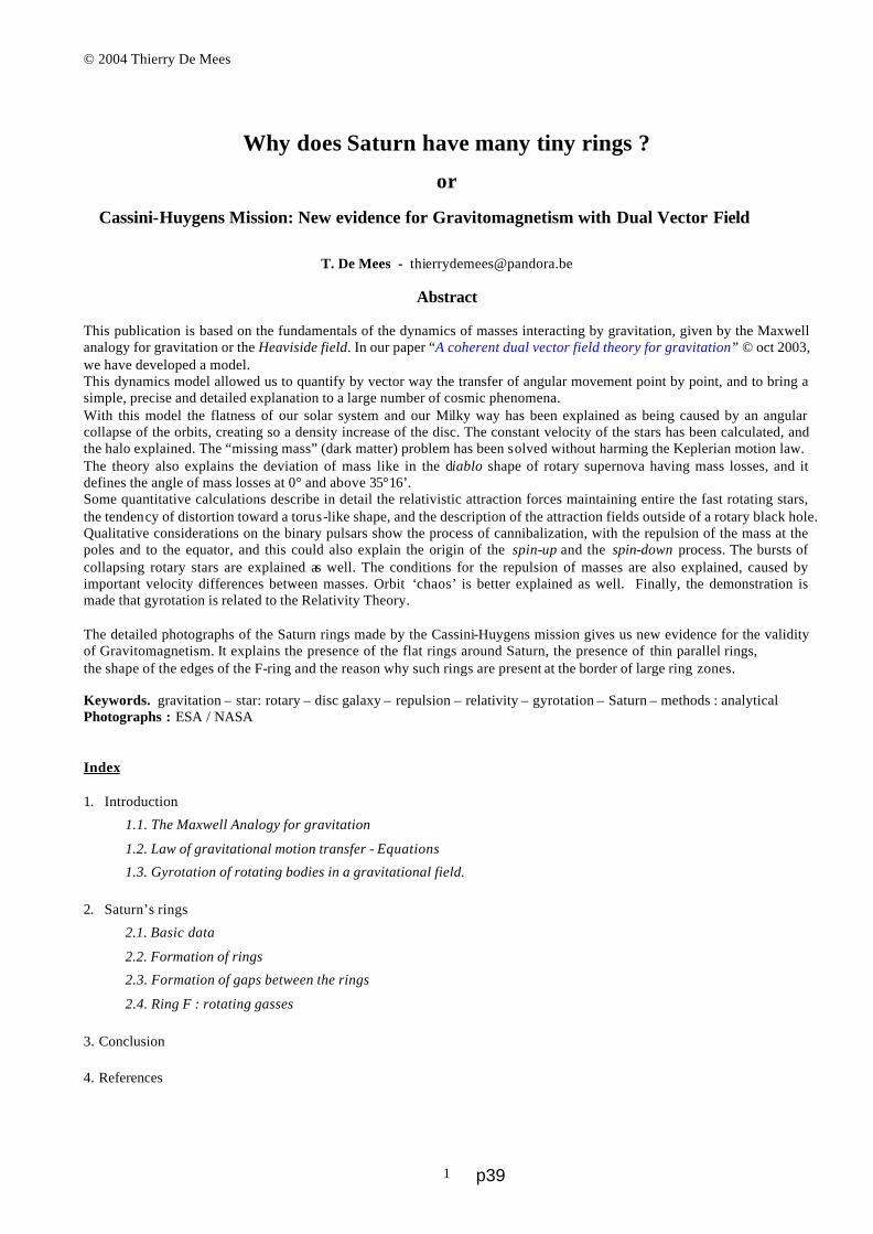
© 2004 Thierry De Mees
1
Why does Saturn have many tiny rings ?
or
Cassini-Huygens Mission: New evidence for Gravitomagnetism with Dual Vector Field
T. De Mees - [email protected]
Abstract This publication is based on the fundamentals of the dynamics of masses interacting by gravitation, given by the Maxwell analogy for gravitation or the Heaviside field. In our paper “A coherent dual vector field theory for gravitation” © oct 2003, we have developed a model. This dynamics model allowed us to quantify by vector way the transfer of angular movement point by point, and to bring a simple, precise and detailed explanation to a large number of cosmic phenomena. With this model the flatness of our solar system and our Milky way has been explained as being caused by an angular collapse of the orbits, creating so a density increase of the disc. The constant velocity of the stars has been calculated, and the halo explained. The “missing mass” (dark matter) problem has been solved without harming the Keplerian motion law. The theory also explains the deviation of mass like in the diablo shape of rotary supernova having mass losses, and it defines the angle of mass losses at 0° and above 35°16’. Some quantitative calculations describe in detail the relativistic attraction forces maintaining entire the fast rotating stars, the tendency of distortion toward a torus-like shape, and the description of the attraction fields outside of a rotary black hole. Qualitative considerations on the binary pulsars show the process of cannibalization, with the repulsion of the mass at the poles and to the equator, and this could also explain the origin of the spin-up and the spin-down process. The bursts of collapsing rotary stars are explained as well. The conditions for the repulsion of masses are also explained, caused by important velocity differences between masses. Orbit ‘chaos’ is better explained as well. Finally, the demonstration is made that gyrotation is related to the Relativity Theory. The detailed photographs of the Saturn rings made by the Cassini-Huygens mission gives us new evidence for the validity of Gravitomagnetism. It explains the presence of the flat rings around Saturn, the presence of thin parallel rings, the shape of the edges of the F-ring and the reason why such rings are present at the border of large ring zones. Keywords. gravitation – star: rotary – disc galaxy – repulsion – relativity – gyrotation – Saturn – methods : analytical Photographs : ESA / NASA Index 1. Introduction
1.1. The Maxwell Analogy for gravitation
1.2. Law of gravitational motion transfer - Equations
1.3. Gyrotation of rotating bodies in a gravitational field. 2. Saturn’s rings
2.1. Basic data
2.2. Formation of rings
2.3. Formation of gaps between the rings
2.4. Ring F : rotating gasses 3. Conclusion 4. References
p39
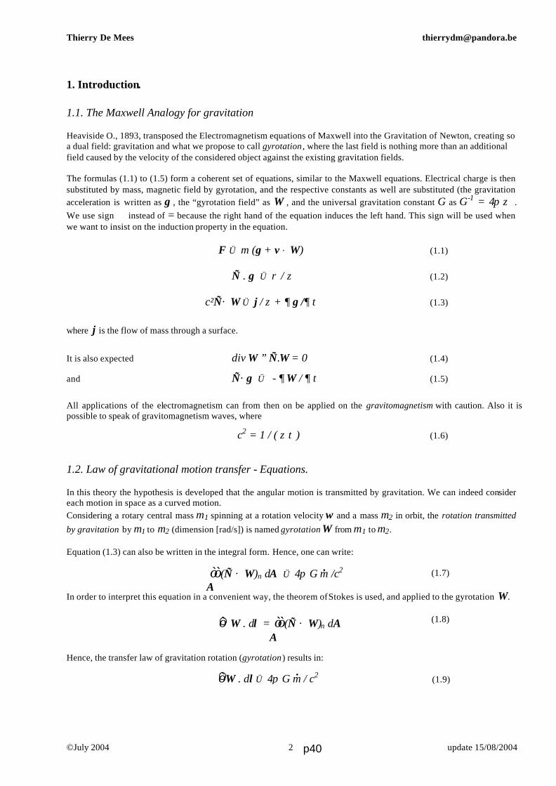
Thierry De Mees [email protected]
©July 2004 update 15/08/2004 2
1. Introduction.
1.1. The Maxwell Analogy for gravitation Heaviside O., 1893, transposed the Electromagnetism equations of Maxwell into the Gravitation of Newton, creating so a dual field: gravitation and what we propose to call gyrotation , where the last field is nothing more than an additional field caused by the velocity of the considered object against the existing gravitation fields. The formulas (1.1) to (1.5) form a coherent set of equations, similar to the Maxwell equations. Electrical charge is then substituted by mass, magnetic field by gyrotation, and the respective constants as well are substituted (the gravitation acceleration is written as g , the “gyrotation field” as Ω , and the universal gravitation constant G as G-1 = 4π ζ ). We use sign ⇐ instead of = because the right hand of the equation induces the left hand. This sign will be used when we want to insist on the induction property in the equation.
F ⇐ m (g + v × Ω ) (1.1)
∇ . g ⇐ ρ / ζ (1.2)
(1.3)
where j is the flow of mass through a surface. It is also expected div Ω ≡ ∇.Ω = 0 (1.4)
and ∇×g ⇐ - ∂ Ω / ∂ t (1.5)
All applications of the electromagnetism can from then on be applied on the gravitomagnetism with caution. Also it is possible to speak of gravitomagnetism waves, where
c2 = 1 / ( ζ τ ) (1.6) 1.2. Law of gravitational motion transfer - Equations. In this theory the hypothesis is developed that the angular motion is transmitted by gravitation. We can indeed consider each motion in space as a curved motion. Considering a rotary central mass m1 spinning at a rotation velocity ω and a mass m2 in orbit, the rotation transmitted
by gravitation by m1 to m2 (dimension [rad/s]) is named gyrotation Ω from m1 to m2. Equation (1.3) can also be written in the integral form. Hence, one can write:
(1.7) In order to interpret this equation in a convenient way, the theorem of Stokes is used, and applied to the gyrotation Ω .
(1.8)
Hence, the transfer law of gravitation rotation (gyrotation) results in:
(1.9)
∫ Ω . dl = ∫∫ (∇ × Ω )n dA A
∫∫ (∇ × Ω )n dA ⇐ 4π G m /c2 A
.
c²∇× Ω ⇐ j / ζ + ∂ g /∂ t
∫ Ω . dl ⇐ 4π G m / c2 .
p40

Thierry De Mees [email protected]
©July 2004 update 15/08/2004 3
1.3. Gyrotation of rotating bodies in a gravitational field. For a sphere, we found:
Fig. 1.1 (1.10) (1.11) For homogeny rigid masses we can write :
(Reference: Eugen Negut, www.freephysics.org) (1.12) The drawing shows equipo- tentials of – Ω .
2. Saturn’s rings. 2.1. Basic data Some basic data concerning Saturn will allo w us to calculate the gyrotation at any point of space.
• diameter at its equator : 120.536 kilometres • mass : 5,69 E+26 kg • rotation period : 10,233 hours
• Saturn’s rings :
Name Distance*
(km) Width (km)
Thickness (km)
Optical Depth
Mass (g)
Albedo
D 66,000 - 73,150 7,150 ? 0.01 ? ? C 74,500 - 92,000 17,500 ? 0.05 - 0.35 1.1 x 1024 0.12 - 0.30
Maxwell Gap 87,500 270 B 92,000 - 117,500 25,500 0.1 - 1 0.8 - 2.5 2.8 x 1025 0.5 - 0.6
Cassini Div 117,500 - 122,200 4,700 ? 0.05-0.15 5.7 x 10²³ 0.2 - 0.4 A 122,200 - 136,800 14,600 0.1 - 1 0.4-0.5 6.2 x 1024 0.4 - 0.6
Encke gap 133,570 325 Keeler gap 136,530 35
F 140,210 30 - 500 ? 0.01-1 ? 0.6 G 164,000 - 172,000 8,000 100 - 1000 10-6 1020 ? E 180,000 - 480,000 300,000 1,000 10-5 ? ?
* The distance is measured from the planet centre to the start and to the end of the ring. 2.2. Formation of rings. Every orbital mass will get a pressure towards Saturn’s equator plane. We consider a prograde orbit (fig.2.1).
4 π G ρ 2 1 r ⋅ (r • ω) c2 5 3 5
Ωint ⇐ ⋅ ω ( ⋅ r2 - ⋅ R2) - Y p r X R
Ωext ⇐ ⋅ - 4 π G ρ R5 ω r ⋅ (ω • r) 5 r3 c2 3 r2
Ωext ⇐ ⋅ ω - G m R2 3 r ⋅ (ω • r) 5 r3 c2 r2
p41

Thierry De Mees [email protected]
©July 2004 update 15/08/2004 4
If vp = r ωp is the orbit velocity of the mass mp , it gets an
acceleration: ap ⇐ vp × Ωp where ap is pointed in a direction, perpendicular on the equipotential path. One finds the tangential component apt and the radial component apr out of (1.11). The acceleration apt always sends the orbit of mp toward the plane of the equator of m in a prograde orbit. The component apr is responsible for an small orbit diameter decrease and a small increase of velocity, due to the law of conservation of energy :
v = (GM/r)-1/2 (2.1)
2.3. Formation of gaps between the rings The gyrotation pressure caused by apt will tend to flatten the rings until almost zero. This is more or less possible as far as the material is exclusively made of solids. With gasses, we will have a different situation, explained in next section. At the beginning, the gyrotation’s angular collapse is causing a high density at every place of the ring because Saturn’s gyrotation pressure pushes the ring to be as thin as possible. At first, the density is more or less uniform, slightly increasing or decreasing at larger or shorter distance from Saturn, depending from the original local density of the cloud around Saturn, before the collapse. After the collapse, the gyrotation forces will keep the ring very thin closer to Saturn, and less thin at larger distances. The following phenomena will occur now, caused by gravitation : the high local density of the ring will force a conglomeration of masses. We get a ring whose section is shown in fig. 2.3 having its own gyrotation fields. The gyrotation from Saturn is not taken in account here, because it gives a quasi uniform extra almost vertical field. In fig. 2.4, we show the gyrotation forces working on the ring, and a field which is perpendicular to it, representing gravitation. Fig. 2.3
Near the edges of the upper side of the ring, a gyrotation force is acting due to the velocity of the edge’s part and its mass, given by equation (1.1). The gyrotation force has got two components, and the vertical one, FΩ y (fig. 2.4) tries to reduce the thickness of the ring, and exactly the same is happening at the down side of the ring, at the same place x, where an upwards FΩ y acts. At the edge however, a greater compression is created by the component FΩ x , which increases the density of the edge. The mass flow density increases as well,
and gyrotation increases, helping the gravitation forces. Indeed, the ring is made of blocks, and gyrotation forces make these blocks really move. Every motion however will have consequences for the energy conservation law between gravitation and centrifugal forces, expressed by (2.1).
y ω Ω mp
apr Ωp
r m α ap apt x
Fig. 2.1
Fig. 2.2 Saturn's A ring
g Ω
Ω
FΩ x FΩ FΩ y
Fig 2.4
p42

Thierry De Mees [email protected]
©July 2004 update 15/08/2004 5
The blocks that move away from Saturn will get an orbit which slows down and the blocks at the other edge of the ring will get a faster orbit velocity. Very probably, the blocks at each edge will get a turbulent double circular motion and consequently endure many collisions (fig. 2.5.a), while the rest of the ring tries to remain in the correct orbit without turbulences. The edges become more compact but turbulent, and probably the blocks become smaller and more numerous because of the many collisions. In section 2.4 , it will become more obvious how we come to this turbulent double circular motion, when we will handle the process with gasses. Even a small change of the edge’s outline, or a small gap between the edge region and the rest of the ring will allow the
gyrotation forces to change it’s shape (fig. 2.5.b) and get opposite gyrotation forces FΩ x at the split point. Slowly but surely, the edge’s shape becomes circular due to the new orientation of the gyrotation forces. Turbulent motions decrease and a more stable tiny ring is created out from the edge, helped by both gravitation and the novel gyrotation forces. When this part has been separated (and the same happened at the other edge of the ring) we get a new shape of the gyrotation equipotentials ’ paths, as shown in fig. 2.6.
Fig. 2.6 The separations reduces the width of the remaining ring. But still, the same process is able to split off another mass of the new formed edges. In this example, the next separated mass will be all nearly as big as the first one. In reality, the size of the new ring is somewhat different : the influence of the first separated tiny ring reduce slightly the compression power of Ω at the new edges of the large ring. Every new separated mass is then successively slightly smaller than the previous one. The result is a succession of separations of ring-shaped masses, which become smaller and smaller the more we reach the centre of the original ring. The larger the separated mass, the larger the gap near it, what means that the average density remains uniform as it was before the separations. 2.4. Ring F : rotating gasses. The shape of a part of the ring F is strange: its looks like drops or clumps; it was thought that it was a succession of tiny moons (fig. 2.6). In fact, we will show below that it is a beautiful demonstration of the gyrotation forces. Let’s start from the assumption that this part of the ring is a gas cloud, or made out of fine particles. The gyrotation acceleration on a particle of the cloud is pointed perpendicularly on the gyrotation :
Ω
Ω
FΩx FΩ FΩ y
Fig 2.5.b
Ω
Fig 2.5.a
p43
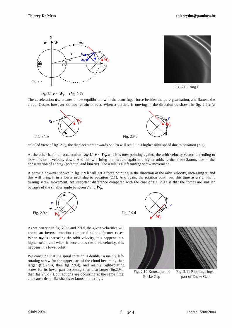
Thierry De Mees [email protected]
©July 2004 update 15/08/2004 6
aΩ ⇐ v × Ωp (fig. 2.7).
The acceleration aΩ creates a new equilibrium with the centrifugal force besides the pure gravitation, and flattens the cloud. Gasses however do not remain at rest. When a particle is moving in the direction as shown in fig. 2.9.a (a
detailed view of fig. 2.7), the displacement towards Saturn will result in a higher orbit speed due to equation (2.1). At the other hand, an acceleration aΩ ⇐ v × Ωp which is now pointing against the orbit velocity vector, is tending to slow this orbit velocity down. And this will bring the particle again in a higher orbit, farther from Saturn, due to the conservation of energy (potential and kinetic). The result is a left turning screw movement. A particle however shown in fig. 2.9.b will get a force pointing in the direction of the orbit velocity, increasing it, and this will bring it in a lower orbit due to equation (2.1). And again, the rotation continues, this time as a right-hand turning screw movement. An important difference compared with the case of fig. 2.9.a is that the forces are smaller because of the smaller angle between v and Ωp. As we can see in fig. 2.9.c and 2.9.d, the given velocities will create an inverse rotation compared to the former cases. When aΩ is increasing the orbit velocity, this happens in a higher orbit, and when it decelerates the orbit velocity, this happens in a lower orbit. We conclude that the spiral rotation is double : a mainly left-rotating screw for the upper part of the cloud becoming then larger (fig.2.9.a, then fig 2.9.d), and mainly right-rotating screw for its lower part becoming then also larger (fig.2.9.a, then fig 2.9.d). Both actions are occurring at the same time, and cause drop-like shapes or knots in the rings.
v Ωp
Fig. 2.9.a
v Ω p
Fig. 2.9.b
v Ωp
Fig. 2.9.c
v
Ωp Fig. 2.9.d
Fig. 2.11 Rippling rings, part of Encke Gap
Fig. 2.10 Knots, part of Encke Gap
Fig. 2.6 Ring F
y ω Ω mp
r ar
m α aΩ at Ωp x
Fig. 2.7
p44

Thierry De Mees [email protected]
©July 2004 update 15/08/2004 7
Concerning the gyrotation of the gas ring itself, it is only causing a radial or an increasing or decreasing orbital movement (fig. 2.9.e), and does not influence the described phenomena. Finally, we should insist on the reason why these ribbed rings are more evidently present at the edges of the rings. The reason has been explained in section 2.3 : the turbulence of the original edges is much higher than in the other parts of the ring, causing smaller particles by collisions and by the more adequate orientations of the gyrotation forces. 3. Conclusion The gyrotation, defined as the transmitted angular movement by gravitation in motion, is a plausible explanation for the formation of the Saturn thin disc, the tiny rings, and the drop-like or ribbed rings. It explains many cosmic phenomena described in : “A coherent dual vector field theory for gravitation” De Mees, T., 2003 as well. 4. References See reference list of : De Mees, T., 2003, A coherent dual vector field theory for gravitation.
Ωp
Fig. 2.9.e
p45
Thierry De Mees
On the dynamics of Saturn's spirally wound F-ring edge.
Described by usingthe Maxwell Analogy for gravitation.
T. De Mees - thierrydm @ pandora.be
Abstract
The F-ring of Saturn shows a spirally wound edge. I have deduced its qualitative behaviour in section 2.4 of “NewEvidence for the Dual Vector Field Theory for Gravitation (Cassini-Huygens Mission)” . These spirals formregular buds with an amplitude and a wavelength. The aim of this paper is to show the relationship between thephysical dimensions of the buds and the orbital velocity of the F-ring's edge.
Keywords: Saturn – gravitation – gyrotation – F-ring.Method: Analytical.
1. The Maxwell Analogy for gravitation: equations and symbols.
For the basics of the theory, I refer to : “A coherent double vector field theory for Gravitation”. The most relevantparts are summarized hereafter. The laws can be expressed in equations (1.1) up to (1.6) below. The electric charge is then substituted by mass, the magnetic field by gyrotation, and the respective constants are
also substituted. The gravitation acceleration is written as g , the so-called gyrotation field as Ω Ω Ω Ω , and the
universal gravitation constant out of G-1 = 4π ζ , where G is the universal gravitation constant. We use sign ⇐instead of = because the right-hand side of the equations causes the left-hand side. This sign ⇐ will be used whenwe want insist on the induction property in the equation. F is the resulting force, v the relative velocity of the
mass m with density ρ in the gravitational field. And j is the mass flow through a fictitious surface.
F ⇐ m ( g + v × Ω Ω Ω Ω ) (1.1)
∇∇∇∇ . g ⇐ ρ / ζ (1.2)
c² ∇∇∇∇× ΩΩΩΩ ⇐ j / ζ + ∂ g /∂ t (1.3)
div j ⇐ - ∂ρ / ∂ t (1.4)
div ΩΩΩΩ ≡ ∇∇∇∇. ΩΩΩΩ = 0 (1.5)
∇∇∇∇× g ⇐ - ∂ ΩΩΩΩ / ∂ t (1.6)
It is possible to speak of gyrogravitation waves with transmission speed c.
c2 = 1 / ( ζ τ ) (1.7) wherein τ = 4π G/c2.
© Nov. 2007 23/11/20071 p46

Thierry De Mees
2. The F-ring.
2.1 Visual properties of the F-ring.
The F-ring is much larger in shape then the many other thin rings. The inside structure is also finer and foggy. It ismade of gasses, which are shaped as spirally wound, regular buds.
A recent photograph by the Cassini-Huygens Mission shows them clearly.Let us call the wavelength L and the radius of the tiny ring rF (see fig. 2.1).
Fig. 2.1 a. F-ring : detail (ESA / NASA) Fig. 2.1 b. F-ring : detail (ESA / NASA)
2.2 Defining the gyrotation field of Saturn and the swiveling of the global ring.
Consider a rotating sphere, enveloped by its gravitation field, and at this condition, we can apply the analogy withthe electric current in closed loop, integrated over the sphere. (Reference: Richard Feynmann: Lecture on Physics)
The result for the equatorial gyrotation Ω at a distance r from the centre of the sphere with radius R is given by
the equation (see “A coherent dual vector field theory for gravitation” equation (4.3) where ω • r = 0 ) :
(2.1)
where ω is the angular rotation velocity of Saturn, R its radius and r the orbital radius of the F-ring. Thisgyrotation field points exacty opposite to the rotation vector of Saturn.
This gyrotation field generates a force on the moving particles in the F-ring.
In my paper “Cassini-Huygens Mission: New evidence for the Gravitational Theory with Dual Vector Field” ,section 2.4 , is explained how we come to small successive rings. In the beginning, there was a cloud aroundSaturn, which rotated around the planet. These individual orbits swivelled all to the equator, due to Saturn'sgyrotation field, and they formed a huge, flat disk.
Just for information, note that in “Swivelling Time of Spherical Galaxies Towards Disk Galaxies” I explained theproces of swiveling, and I calculated the swiveling time for a disk galaxy. Adapted for the Saturn's disk, this gives:
© Nov. 2007 23/11/20072
Ω = G m Rr c
2
3 25ω
L / 2
2 rF
p47
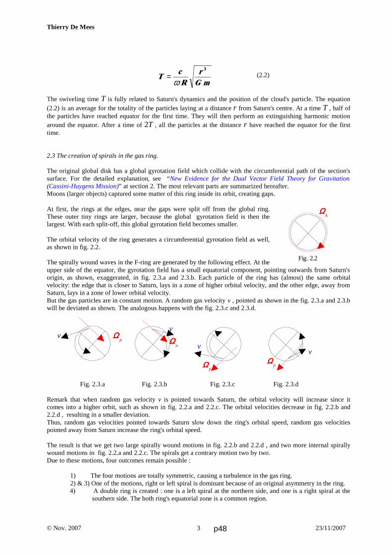
Thierry De Mees
(2.2)
The swiveling time T is fully related to Saturn's dynamics and the position of the cloud's particle. The equation(2.2) is an average for the totality of the particles laying at a distance r from Saturn's centre. At a time T , half ofthe particles have reached equator for the first time. They will then perform an extinguishing harmonic motionaround the equator. After a time of 2T , all the particles at the distance r have reached the equator for the firsttime.
2.3 The creation of spirals in the gas ring.
The original global disk has a global gyrotation field which collide with the circumferential path of the section'ssurface. For the detailed explanation, see “New Evidence for the Dual Vector Field Theory for Gravitation(Cassini-Huygens Mission)” at section 2. The most relevant parts are summarized hereafter.Moons (larger objects) captured some matter of this ring inside its orbit, creating gaps.
At first, the rings at the edges, near the gaps were split off from the global ring.These outer tiny rings are larger, because the global gyrotation field is then thelargest. With each split-off, this global gyrotation field becomes smaller.
The orbital velocity of the ring generates a circumferential gyrotation field as well,as shown in fig. 2.2.
The spirally wound waves in the F-ring are generated by the following effect. At theupper side of the equator, the gyrotation field has a small equatorial component, pointing outwards from Saturn'sorigin, as shown, exaggerated, in fig. 2.3.a and 2.3.b. Each particle of the ring has (almost) the same orbitalvelocity: the edge that is closer to Saturn, lays in a zone of higher orbital velocity, and the other edge, away fromSaturn, lays in a zone of lower orbital velocity.But the gas particles are in constant motion. A random gas velocity v , pointed as shown in the fig. 2.3.a and 2.3.bwill be deviated as shown. The analogous happens with the fig. 2.3.c and 2.3.d.
Fig. 2.3.a Fig. 2.3.b Fig. 2.3.c Fig. 2.3.d
Remark that when random gas velocity v is pointed towards Saturn, the orbital velocity will increase since itcomes into a higher orbit, such as shown in fig. 2.2.a and 2.2.c. The orbital velocities decrease in fig. 2.2.b and2.2.d , resulting in a smaller deviation.Thus, random gas velocities pointed towards Saturn slow down the ring's orbital speed, random gas velocitiespointed away from Saturn increase the ring's orbital speed.
The result is that we get two large spirally wound motions in fig. 2.2.b and 2.2.d , and two more internal spirallywound motions in fig. 2.2.a and 2.2.c. The spirals get a contrary motion two by two.Due to these motions, four outcomes remain possible :
1) The four motions are totally symmetric, causing a turbulence in the gas ring. 2) & 3) One of the motions, right or left spiral is dominant because of an original asymmetry in the ring.4) A double ring is created : one is a left spiral at the northern side, and one is a right spiral at the
southern side. The both ring's equatorial zone is a common region.
© Nov. 2007 23/11/20073
v ΩΩΩΩp
v
ΩΩΩΩp
v ΩΩΩΩ
p
v
Ω Ω Ω Ωp
Fig. 2.2
Ω Ω Ω ΩA
TcR
rG m
=ω
3
p48

Thierry De Mees
We expect that 1) is the starting situation, and that one of the other situations is following after that. For gas rings,the latter outcome should be more likely.
2.4 Further qualitative dynamics' study of the double twisted F-ring
Let us study the global motion of the gasses in the F-ring more in detail. In fig. 2.4 , the F-ring is shown as thesection of a tore, with different orbital radii r i.
Fig. 2.4 : section of the F-ring, schematic view. The orbital radii , orbitalvelocities' gradient, gyrotations, the pressure gradient and the global motion
inside the cloud are shown.
A section is shown with velocities vi , perpendicular to the paper and pointing away from the reader. Due to thefinite size of the section, the orbital velocities follow the rule:
(2.3) and because
Saturn's gyrotation ΩS will induce an acceleration to the left for the whole section, and tend to extend the left sideof the section to the left, where the velocities are higher. This will flatten the tore.
Due to the orbital velocity of the F-ring, a circular (rather elliptical) gyrotation ΩF is created as well. Using (1.1) ,where the gravitational term, which is pointing to the section's centre can be omitted, it is clear that for thecorresponding pressures, we get :
© Nov. 2007 23/11/20074
vG mrii
= v v v v v1 2 3 4 5> > > > r r r r r1 2 3 4 5< < < <
p p p p p1 2 3 4 5> > > >
ΩF
p1 p5
p2 p4
p3
p3
p2 p4
p1 p5
v3
v2 v4
v1 v5
v1 v5
v2 v4
v3
r1
r2
r3
r4
r5
r4
r5
r5
r4
r1
r2
r3
ΩS ΩS ΩS ΩS
ΩF
p49

Thierry De Mees
since ai are the corresponding accelerations according (1.1) : (2.4)
In superposition of the effect, shown in fig. 2.3 , we get another effect: the left pressures will induce a motion asshown in fig. 2.4 by the double arrows. This motion is an acceleration which can be deduced from (2.4). Therefore we need the value of the orbital
velocity which follows from (2.3), and the gyrotation ΩF . In “A coherent double vector field theory for Gravitation” , section 13, it follows that :
(2.5) or (2.6)
where vF can be v1 for example. The acceleration becomes: (2.7)
Indeed, the value of the gyrotation ΩF slightly varies from place to place, depending from the choice of vi . At theleft side of fig. 2.4 it is larger than at the right side.
In (2.7) , ρ is the density of the cloud, supposed to be homogene for simplicity, which depends also from itstemperature. This parameter is not within the scope of this paper.Although this acceleration might appear very small, the actual velocity of the double spiral became verysignificant after many years. It is acceptable to assume that at this moment, the maximum possible dynamics havebeen reached in order to maintain the spirally wound cloud together by their own gravitation forces.In the section hereafter, we try to find the relationship between the buds' shape and the velocities in the F-ring.
2.5 Relationship between the buds shape and the velocities in the F-ring.
The acceleration of (2.7) will result in a double spiral, one in the northern part, one in the southern, with mutuallyinversed rotations. At the surface of the cloud, a finite curved velocity will be reached, creating so a centripetalforce, which will be in balance with the gravitational force.Let us call vF,Ω the elliptical velocity of the spiral motion, in the plane of the section in fig. 2.4 , which has beencreated by (2.7). For a specific point P at the extremity of the cloud, this velocity must be in balance as follows:
(2.8)
The left hand is the integration of the gravitation field of a infinite plain cylinder for a point P at its surface. Sincethis integral is hard to find, I will use an artifact.
The infinite plain cylinder can be approached by a succession of spheres, while guarantying the same volume andthus masses. Since the gravitation field of a sphere is easy to find (point mass equivalence), the result is then easyto find and fairly correct.
Fig. 2.5 : approximation of a long cylinder by spheres.
© Nov. 2007 23/11/20075
a vi i F= × Ω
24
2π πr
Gc
m vF F F iΩ = Ω FF iG r v
c= 2
2
π ρ
a G rvcF F,Ω = 2 1
2
2π ρ
Gmr
v
rF
F
F
F
d ,
2
2
z = Ω
P rF
l
p50

Thierry De Mees
To guaranty a same volume, it is needed that : (2.9)
It can be found, that using the artifact of fig. 2.5 , the following integral is found for the left hand of (2.8).
(2.10)
The series converge very quickly, so that the equivalence of the tore and the infinite plain cylinder becomesacceptable.Solving the figures part, and using the right hand of (2.8) , this gives :
(2.11)
This is the maximum value of the elliptical velocity of the double spiral motion in the section of fig. 2.4.
There is also another phenomena to consider. The time t , needed for a particle to describe a full spiral cycle, mustbe equal to the time needed (by the same particle) to fulfill a complete orbital wavelength L (see fig 2.1).
Hence, or, with (2.11) : (2.12)
The parameter v t,Ω is the orbital velocity of the double spiral motion, with exception of the dragging orbitalvelocity. Indeed, it is possible that the whole spiral F-ring is not only screwing through the vacuum, but is also partiallydragged as a whole and that v t,Ω is only a part of the total average orbital velocity (v3 for example).
(2.13)
The dragging effect can be observed, and both (2.11) and (2.12) can be verified if the density of the F-ring isknown.
2.6 Creation of an elliptic halo's at the inner edge of the F-ring.
Although we came to the equations (2.11) , (2.12) and (2.13) as a steady state, indeed these velocities are stillunder the influence of equation (2.7). Some particles will be lifted farther away from the F-ring, and because of the
increase of rF and the decrease of ρ , the acceleration aF,Ω will decrease quickly as well. It is then probable that adouble halo would be created at the left side of the F-ring in fig. 2.4 (inner edge of the ring) which is a cloud thatcontinuously is pumping gasses from the right side to the left side, and filling the gap next to (left from) the F-ring.At the equator, the gasses have no specific rotation velocity and can thus be attracted again by the F-ring. There exists a phenomena that avoids the adoption of these gasses by the next tiny ring at the left of the F-ring,which will be explained in a later paper.
© Nov. 2007 23/11/20076
4
3rF = l
Gmr
G r
i
F
FF
i
d2 2 3 2
1
4
31 2
1
14
3
z ∑= +
+ FHGIKJ
FHG
IKJ
F
H
GGGGG
I
K
JJJJJ
=
∞
π ρ
v r GF F, ,Ω = 2 57 ρ
tr
vL
vF
F t
= =2π, ,Ω Ω
v v vdrag t= −3 ,Ω
v L Gt , ,Ω = 0 41 ρ
p51
Thierry De Mees
3. Discussion and conclusion.
Deduced from the qualitative gyrotation analysis, we come to a double spirally wound F-ring, one in the northernpart, one in the southern part, with mutually inversed rotations.The equations (2.11) , (2.12) and (2.13) describe the relationship between the double spiral dynamics and the buds'geometry of the F-ring. Some of these parameters are public yet, but some parameters should be knownsomewhere at NASA/ESA. Remark that these equations are independent from Saturn's parameters, because we calculated the equilibrium atthe edge of the F-ring's cloud itself, assuming a maximal possible elliptical velocity vF,Ω . Thus, these equationsare purely classical physics.When all the parameters of (2.11) , (2.12) and (2.13) are known, we have again an indirect proof (to myfrustration) of the Gyrogravitation Theory (= the Maxwell Analogy for Gravitation) which has been suggested byHeaviside at the end of the 19th century. Indeed, gravitation only cannot fully explain the double spirally woundparts of the F-ring. In this paper, the most important equation, which is fully related to the gyrotation fields, is given by (2.7).However, it will probably be hard to detect this property visually because the initial dynamics has evolved to theactual steady state dynamics, which doesn't show this acceleration any more.
4. References and interesting literature.
1. Einstein, A., 1916, Über die spezielle und die allgemeine Relativitätstheorie.
2. Feynman, Leighton, Sands, 1963, Feynman Lectures on Physics Vol 2.
3. Heaviside, O., A gravitational and electromagnetic Analogy, Part I, The Electrician, 31, 281-282 (1893)
4. Jefimenko, O., 1991, Causality, Electromagnetic Induction, and Gravitation, (Electret Scientific, 2000).
5. De Mees, T., General insights for the Maxwell Analogy for Gravitation.
Solar-, planetary- and ring-system's dynamics.
Fast spinnings stars' and black holes' dynamics.
Spherical and disk galaxy's dynamics.
© Nov. 2007 23/11/20077 p52
3The UltimateProbation Tests for Gyrotation
Replacing an old-fashion theory into a new one sometimes is like David fighting against Goliath. The two following papers go about the ultimate tests, upon which the old General Relativity Theorywas based : the unexplained remaining perihelion advance of Mercury, the bending of the lightgrazing the Sun, the changing clock rates, and later, the lifetime of very fast mesons.
Clocks are not always following the Special Relativity Theory, and the General Relativity Theory isfairly close, but does not totally comply with Gravitomagnetism.Surprisingly, Mercury's unexplained perihelion advance occurs as follows: our Milky Way exercisesa gravitomagnetic field upon our Sun and on its turn, the Sun's gyrotation works in upon Mercury.The bending of the light grazing the Sun complies with Gravitomagnetism when one realizes thatthe light beam's Gravitomagnetism will perceive all matter approaching at the speed of light.Also the lifetime of very fast mesons simply follows from a physical gyrotational compression.Discover now the obviously successful approach of Gravitomagnetism!
p53

Did Einstein cheat ?or
How Einstein solved the advance of Mercury’s perihelionand the gyrotational bending of light.
Described by :Gravitomagnetism.
T. De Mees - [email protected]
Abstract
Since one century, Gravitation has been in the spell of Einstein's Relativity Theory. Although during decades,dozens of scientists have provided evidences for the incorrectness of this theory. And often successfully, butwithout finding a sympathetic ear. Here we will discover what is wrong with the theory, and what brings a lot ofscientists -in spite of that- to not dump it. We will not only discover that the Relativity Theory of Einstein is atricked variant of the authentic Gravitation Theory, but we will also be able to form an idea about how and whyEinstein did this. Did Einstein cheat? is no attack on the person of Einstein, or on its working method. For that thereasons are too few. But it is a beautiful example, in these times, of a too long idolatry of a theory, just like it wasthe time before Galileo in astronomy and the time before Vesalius in medicine. Most remarkable is that the correctGravitation Theory is an older theory than the Relativity Theory itself. In Did Einstein cheat? both theories areexamined and compared, put in their historical and scientific context, and applied on some essential physicalphenomena: the progress of the perihelion of Mercury and the bending of the light close to the sun.
Key words : Mercury's perihelion advance, bending of light, gravitomagnetism, relativity theory.Method : analytical.
Index
1. Introduction: two competitive models. 1905: the birth of a new vision / 1893: the consolidation of an old
concept / Has the last word been said ?
2. The Maxwell Analogy for Gravitation: a short overview.
3. The Maxwell Analogy for Gravitation examined by Oleg Jefimenko. The generalisation of the Maxwell
Analogy / The Maxwell Analogy forms a coherent gravitation theory / Relativistic and non-relativistic clocks.
4. The Maxwell analogy for gravitation examined by James A. Green. The Relativity Theory for Gravitation and
the Maxwell Analogy are almost identical / The speed of light does not originate from c2 = 4 (ε µ )-1
5. General Relativity Theory: a dubious calibration? The Mercury’s perihelion advance/ The bending of star light
grazing the sun / Discussion
6. Comparison with the Maxwell Analogy. The advance of Mercury’s perihelion and the Milky Way / The bending
of star light grazing the sun
7. Has the Relativity Theory era been fertile so far?
8. Conclusion: Did Einstein cheat ?
9. References and interesting literature.
© 28 Dec. 2004 – 2010 Update 15 Oct. 20101 p54

1. Introduction: two competitive models.
1905: the birth of a new vision
Almost hundred years ago, a milestone was put in the history of science: the special Relativity Theory arose fromEinstein’s brain around 1905, as a result of a number of perceptions which could simply not be explained.
The first basic idea which has put the scientific world on its head was the concept “relativity of the speed”. Thisbasic idea was able to explain the Lorentz contraction that appeared to follow from the Michelson-Morleyexperience. Out of that the Special Relativity Theory arose. A number of scientists was soon won for the idea. Thenext logical step was of course acceleration. Immediately the next problem arose: are gravitation mass andgravitation acceleration different from inertial mass and inertial acceleration? If both could be equated, the waylay open for the development of the “relativity of the acceleration”. But by applying the concept “relativity of theacceleration” on gravitation, Einstein reached the finding that an object falling to a planet, remarkably enoughseems weightless. How could this be united with the fact that masses have a weight?
The philosophical solution came shortly with the “thought experiments” of Einstein: if one cannot discover thedifference between on the one hand someone who stands on the ground in the gravitation field and in this wayexperiences a weight, and on the other hand someone in the space in a lift going upwards, both situations must beidentical. The equivalence of acceleration and weight was shown that way. An elementary mass which is fallingunder the influence of gravitation (and in fact seems weightless) moves according to “weightlessness lines”,usually called “world lines”. Those “weightlessness lines” can describe curved coordinates, and perhaps one canstate that the universe is curved as well. With the aid of a maths expert, Marcel Grossman, Einstein has developeda mathematical model in which a gravitation universe was created, and in which coordinates became not fixed andstraight like in a traditional coordinate system, but could be chosen freely, according the curved “weightlessnesslines”. The logic of this mathematical model lies in the extension of the concept relativity of coordinate systems.
What is considered as brilliant to the theory is moreover that the starting point is generalised but very concise, inthe form of Einstein's field equations. These equations are appropriate on matter, provided that solutions of thefield equations are chosen with care, including the choice of the integration constants. It also seemed to concordwell with the earlier knowledge of the universe, which was rather limited compared to today.
However, we suspect Einstein to have developed a mathematical model that describes only a small part of theknown universe, particularly a part of our solar system that is extrapolated to the complete universe. Moreover, thefragment which in appearance is correct for our solar system is tricked. Soon we see why.
In the viewpoint of mathematicians there is no problem developing a magnificent mathematical theory, which isconcise, very general and beautiful, even if it is verified to be complex solving it in detail. If it can then be appliedon a physical concept, their satisfaction is infinitely large. One mathematical equation can then become thefundament of a universe of which only one fraction was physically observed. Though, that theory offers then thepossibility of setting up the most fabulous speculations, based on each possible solution of that single set ofmathematical equations.
1893: the consolidation of an old concept
Twelve years before the Special Relativity Theory saw the daylight, more than a century ago, knowledge ofelectromagnetism had reached a summit when Oliver Heaviside[5],[4], an autodidact, transformed the laws ofelectromagnetism in a few compact equations, the (wrongly) so-called laws of Maxwell.But as well as this less remarked contribution of Heaviside, also the work concerning the analogous MaxwellEquations for Gravitation became almost forgotten. Heaviside settled in 1893 that the Newton law of gravitationlooked remarkably much like the force law for electric charges. Would it be possible that the gravitation acts thesame way as electromagnetism does? Does there exist something like magnetic gravitation? Heaviside could notprove it, because around 1900 the knowledge of our universe was strongly limited. But he suggested that massworked similarly as charges do, and that two constants exist for Gravitation, analogously to electromagnetism, insuch way that the universal gravitation constant and the speed of light remain linked. The result was a set ofidentical equations -in shape- to these of Maxwell, such as we will discover in next chapter. The challenge whichEinstein had faced, namely to calculate the unexplained part of the Mercury’s perihelion advance of 43 arc
© 28 Dec. 2004 – 2010 Update 15 Oct. 20102 p55
seconds per century, did fade the proponents of the Heaviside theory. One could not get this deviation calculatedby means of the Maxwell Analogy, because with the knowledge of that time, only 1/12th of it could be found[5]!Einstein himself made an attempt using the Maxwell Analogy for gravitation by means of an unnoticedpublication[5], but discovered the problem probably later on. The Relativity Theory seemed to be the onlyexpedient to a solution.
Has the last word been said?
In the dispute which arose between the traditional scientists who consider Maxwell’s Equations as the ultimatetheory to explain gravitational phenomena, and the proponents of the universal Relativity Theory for Gravitationthere are two elements to look at. First, the perception of cosmic phenomena is achieved by mains of collectedelectromagnetic waves such as light and X-rays. These are nicely described by the Relativity Theory, whichgeneralises the bending of these rays to the bending of the space. This tends at the first sight to the benefit of theRelativity Theory. The second element is that the difference between both theories is so small, that the Maxwellequations are considered by the “Relativists” as a good approach of the “correct” Relativity Theory. Moreaccurately, the terms with factors c0 (called “Newtonian solution”) and c2 (called “Post- Newtonian solution of thesecond order”) are seen as a 2nd order approach of the relativistic series development.
For the engineer however, the Relativity Theory of Einstein is not practical this way: the theory tries explaininghow we see things after distortion by gravitation rather than what happens in reality. It is to a great extent alsophilosophical and very general. In the limit, we could state that the Relativity Theory is an Optics Theory whichtakes into account gravitation. And even if the Relativity Theory would come further that the description of lightbehaviour, it is at the cost of an enormous effort of calculations.
As last item we state that the Relativity Theory has proved remarkably little, and what is proved, remains the onlybasis which makes the theory stands or falls: the advance of Mercury’s perihelion which is not completelyexplained by the traditional laws of Newton. When applying the Relativity Theory, the observed deviation of 43arc seconds accords perfectly with the calculated value. And also the bending of the light of stars near the sun isperfectly explained by the Relativity Theory. What could then possibly be wrong with the Relativity Theory?
Oleg Jefimenko has another look on the problem. This scientist and professor at the University of West-Virginiahas developed the suggestion of Heaviside[4] in a coherent Gravitation Theory. Oliver Heaviside wrote downanalogous Maxwell Equations for Gravitation as those for electromagnetism, and examined these further. Indeed,the Maxwell Equations form a correct description of electromagnetic waves. Why wouldn't we test this concept asa model for gravitation?
Oleg Jefimenko’s[5] many years of specialisation in the field of electromagnetism did revive the old suggestion ofHeaviside, and in this way his vision was analysed in detail. He demonstrated that not only the Relativity Theorywas able to describe the consequences of the finite speed of light, and therefore the delay which appears. Thephenomena can be described likewise, if not better, by means of the Maxwell Equations. Jefimenko proves thatthe analogous laws of Maxwell, as an extension of Newton’s laws, provide a complete coherent theory ofgravitational dynamics. But his description of the theory is for the rest mainly restricted to a number of theoreticallaboratory applications. However, very interesting is the study concerning pretended relativistic clocks. Jefimenko shows here that therelativistic property of clocks depends on the composition and the mechanism of the clock, and that relativisticclocks such as (perhaps) the atom is rather incidental than a rule. This means therefore that clocks can berelativistic or not, by concept. In the third chapter we will have a word concerning these clocks.In my work “A coherent double vector field theory for Gravitation” [7] of 2003, I have demonstrated a long range ofapplications on the cosmos, based on the Maxwell Equations for Gravitation. We come back to it soon.
In the second chapter we will discover the Maxwell equations for Gravitation. This theory is then described in thethird chapter within the framework of Jefimenko’s findings. He was able to describe gravitation as a theory whichincorporates the laws of dynamics into a whole, what nobody had accomplished so far. The fourth chapter describes what by James A. Green has discovered. The unexpected observation which we willmake, discredits the exactness of the Relativity Theory significantly, and opens a number of question marks.Finally we will make an amazing observation by applying the Maxwell equations correctly on the progress ofMercurius’ perihelion and on the bending of the stars light grazing the sun.
© 28 Dec. 2004 – 2010 Update 15 Oct. 20103 p56
2. The Maxwell analogy for gravitation: a short overview.
Electromagnetism is very well known, and the many studies about it have excluded each misleading, especiallythanks to the large energies that accompany these fields. Oliver Heaviside suggested the Maxwell analogy forgravitation. Several scientists have examined this theory in depth, of whom the most important is Oleg Jefimenko,which has obtained breathtaking conclusions with regard to the gravitation theory.
The deduction follows from the gravitation law of Newton, taking into account the transversal forces which resultfrom the relative speed of masses. The laws can be expressed in equations (2.1) up to (2.6) below.
Equations (2.1) till (2.6) below form a coherent range of equations, similar to the Maxwell equations. The electriccharge is then substituted by mass, the magnetic field by gyrotation, and the respective constants are also
substituted (the gravitation acceleration is written as g , the so-called gyrotation field as Ω Ω Ω Ω , and the universal
gravitation constant out of G-1 = 4π ζ , where G is the "universal" gravitation constant. We use sign ⇐ insteadof = because the right-hand side of the equations causes the left-hand side. This sign ⇐ will be used when wewant insist on the induction property in the equation. F is the resulting force, v the speed of mass m with density
ρ .F ⇐ m ( g + v × Ω Ω Ω Ω ) (2.1)
∇∇∇∇ . g ⇐ ρ / ζ (2.2)
(2.3)
where j is the mass flow through a fictitious surface. The term ∂ g/∂ t is added for same the reasons such asMaxwell did: the compliance of formula (2.3) with the equation
(2.4)
It is also expected that: div ΩΩΩΩ ≡ ∇∇∇∇. ΩΩΩΩ = 0 (2.5)
and ∇∇∇∇× g ⇐ - ∂ ΩΩΩΩ / ∂ t (2.6)
All applications of electromagnetism can then be applied with prudence on the gyrogravitation. Also it is possibleto speak of gyrogravitation waves with transmission speed c.
c2 = 1 / ( ζ τ ) (2.7)
wherein τ = 4π G/c2.
The laws of Maxwell are not always interpreted correctly and entirely. In the following chapter we examine thelaws of Maxwell, developed by Oleg Jefimenko, with some surprising results.
3. The Maxwell analogy for gravitation examined by Oleg Jefimenko.
The generalisation of the Maxwell analogy
The Maxwell equations suggest that it is possible obtaining an induction between an electric field and a magneticfield and the other way round. Oleg Jefimenko correctly points out that always must be kept in mind that only amoving charged particle, such as the electron, can eventually be the cause of such an induction and not a field byitself. This allows to stay with our both feet on the ground, and not to formulate wild speculations withoutreflection, by manipulating the Maxwell equations: only charges can arouse these fields. Depending of the fact ifthe speed or rather the acceleration is constant, several magnetic or electric fields can be generated. The samehappens with masses. Gravitation fields act analogously to electric fields and gyrotation fields act analogously tomagnetic fields. Both fields are aroused by stationary, steadily moving, or accelerating masses.
© 28 Dec. 2004 – 2010 Update 15 Oct. 20104
c² ∇∇∇∇× ΩΩΩΩ ⇐ j / ζ + ∂ g /∂ t
div j ⇐ - ∂ρ / ∂ t
p57
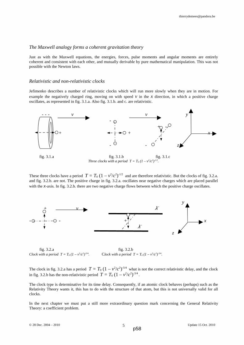
The Maxwell analogy forms a coherent gravitation theory
Just as with the Maxwell equations, the energies, forces, pulse moments and angular moments are entirelycoherent and consistent with each other, and mutually derivable by pure mathematical manipulation. This was notpossible with the Newton laws.
Relativistic and non-relativistic clocks
Jefimenko describes a number of relativistic clocks which will run more slowly when they are in motion. Forexample the negatively charged ring, moving on with speed v in the x direction, in which a positive chargeoscillates, as represented in fig. 3.1.a. Also fig. 3.1.b. and c. are relativistic.
fig. 3.1.a fig. 3.1.b fig. 3.1.cThree clocks with a period T = T0 (1 – v2/c2)-1/2.
These three clocks have a period T = T0 (1 – v2/c2)-1/2 and are therefore relativistic. But the clocks of fig. 3.2.a.and fig. 3.2.b. are not. The positive charge in fig. 3.2.a. oscillates near negative charges which are placed parallelwith the x-axis. In fig. 3.2.b. there are two negative charge flows between which the positive charge oscillates.
fig. 3.2.a fig. 3.2.bClock with a period T = T0 (1 – v2/c2)-5/4. Clock with a period T = T0 (1 – v2/c2)-3/4.
The clock in fig. 3.2.a has a period T = T0 (1 – v2/c2)-5/4 what is not the correct relativistic delay, and the clockin fig. 3.2.b has the non-relativistic period T = T0 (1 – v2/c2)-3/4 .
The clock type is determinative for its time delay. Consequently, if an atomic clock behaves (perhaps) such as theRelativity Theory wants it, this has to do with the structure of that atom, but this is not universally valid for allclocks.
In the next chapter we must put a still more extraordinary question mark concerning the General RelativityTheory: a coefficient problem.
© 28 Dec. 2004 – 2010 Update 15 Oct. 20105
- - - v v y -
+ - + + x
- - z
y+ v λ−
- - + x λ−
z
p58

4. The Maxwell analogy for gravitation examined by James A. Green.
The Relativity Theory for Gravitation and the Maxwell analogy are almost identical
Not only specialists in universities or docents are able fulfilling new contributions. This is illustrated in thischapter. James A. Green has made, with self study, a number of analyses concerning the Relativity Theory. As anengineer he has been interested in the viability of theories too, not only in the theoretical considerations of it. Whathe discovered is very astonishing. He started with the general mathematical expression of the Relativity Theory,and cut it off after the second order (Post-Newtonian approximation of 2nd order; the usual abbreviation is: PN2).Higher orders are not significant. By working out these expressions and fill in Einstein’s equations, he obtains:
c2 = 4 / ( ζ τ ) (4.1)
or, written in usual symbols from electromagnetism: c2 = 4 / (ε µ )
Green further shows that the 2nd order Post-Newtonian solution of the Relativity Theory (this is a time - and place-dependent differential equation) has in fact a well-known solution: the extended time-dependent Maxwellequations, expressed in potential fields:
2 φ = ρ / ζ (4.2)
2 A = τ j (4.3)
ΩΩΩΩ = ∇ = ∇ = ∇ = ∇× A (4.4)
g = - ∇∇∇∇φ - ∂ A /∂ t (4.5)
The coordinates of these potential fields are to be taken locally in time and place. The operator is a four-
coordinate vector made from the three-coordinate operator ∇∇∇∇ in a place x, y, z , and gets as fourth coordinate the
negative partial time derivative - ∂ /∂ t. For masses with low speeds and in the case of stationary situations theabove equations are valid, because the time delay of the field does not have be taken into account. Green actually found these equations out of the Einstein’s field equations, but in which c2 apparently should be
replaced by 4 (ζ τ )-1 at a certain step, in order to get an equivalence of both theories (written in usual symbols
from electromagnetism: c2 = 4 (ε µ )-1).
The speed of light does not originate from c2 = 4 (ε µ )-1
At further development of the equations (4.2) till (4.5) and when infilling in (4.1), Green finds an impossibility.The next expression is, as a matter of fact, found:
4 div j = - ∂ρ / ∂ t (4.6)
what is contradictory with the continuity equation (2.4).
Because of this, we can perfectly say that the General Relativity Theory is not consistent with itself. And theinconsistence is not just an insignificant approximation error, neither finds its cause in cutting-off higher orders ofa serial expansion. The difference is much more significant!
A second proof is also introduced by Green. The Lorentz gauge (that is believed to be at the basis of solutions, inaccordance with the cosmos) for the Relativity Theory is given by equation:
c2 div A = - ∂ φ / ∂ t (4.7)
© 28 Dec. 2004 – 2010 Update 15 Oct. 20106 p59

This equation also brings Green right to (4.6). Normally of course, we expect the expression (2.7) to define the speed of light in the Maxwell equations. TheRelativity Theory can possibly give a very general and interesting general picture of how light goes in its work inthe universe, but it is definitely not exact.
5. General Relativity Theory: a dubious calibration?
Earlier, we have forgotten to explain a step. The general Relativity Theory needs control points. A first controlarea is that at non-relativistic speeds, the theory reduces itself to the Newton theory, as far as we talk about ourplanetary system. A second control area would have been the Lorentz gauge. But above, we saw that the Lorentzgauge is no correct basis to build a theory upon that is entirely correct. However the correctness of the theory isexamined at two measurable phenomena in our solar system: the Mercury’s perihelion advance and the bending ofstar light grazing the sun. First, we describe these control points, and try in the next chapter to find an explanationand a solution to the problem.
The Mercury’s perihelion advance.
It is perhaps not occasional that Mercury’s perihelion advance is for Einstein the reference to justify the GeneralRelativity Theory. Indeed, the issue remains whether Einstein simply has compared the result of the theory to themeasured values, or inversely has harmonized the theory with these figures. In the last case we can speak of acalibration. The Newtonian control calculation of the astronomic values of the perihelion advance was performedby Leverrier in 1859, and was reassessed and improved by Newcomb in 1895. The interpretable advances ofMercury’s perihelion are due to:
1. the progress of the equinox, which explains 5025” per century;2. the perturbation by the planets for total of 526”,7 per century.
Unexplainably compared with the overall astronomic observation is a surplus of 43” per century.
Einstein[1] finds, using the Relativity Theory, a advance excess δ in the form:
(5.1)
with a the half large axis of the elliptic orbit of the planet, T the period, and e the eccentricity of the elliptic orbit.
These values can be found by astronomic observation, and Einstein obtains then δ = 43” . And with this result afirst proof is provided (bad tongs claim: the first calibration realised) for the General Relativity Theory.
But in order to define a curve accurately, one still needs at least a third calibration point. We find the thirdcalibration point in the bending of the star light grazing the sun.
The bending of star light grazing the sun.
When a light ray grazes the sun it is supposed to be bent because ofthe attraction between both masses. The deviation angle was given
by Einstein in 1911 being θN =0,875”Rz/r what was exactly thesame value as with the Newton calculation, and which was wrong.After a number of failed attempts between 1911 and 1914 formeasuring the bending (one pretends that there were no results
known) Einstein brought out the general Relativity Theory in 1915, which gave as a result for the angle the double
value of the Newton one: θE =1,75”Rz/r. Observation is difficult because of the strong sunrays, but at a total
sun eclipse one finds a value close to the relativistic value θE . With radio waves, measuring can be done during all
© 28 Dec. 2004 – 2010 Update 15 Oct. 20107
θ ∆ r
Rz fig.5.1
δ = 24 π 2 a 2 T 2 c 2 (1-e2)
p60

the year, and the value is confirmed near the sun’s poles[8]. However, it is observed that there is a slight deviation
from value θE the more the rays are closer to the equator, whereas the Relativity Theory does not explain this.Furthermore, no consistent results are found.
Discussion
We see therefore that the wrong Lorentz gauge nevertheless finds a correct solution for Mercury’s perihelion andfor the bending by the sun. It is as if twocurves, with the same calibration asymptote(the theory of Newton) and the same twocalibration points (Mercury’s perihelionadvance and the bending of light) have arisen.Although several theories can be quite similar,only one theory will deserve more credit thanthe others. The question is only: which one?Therefore we preferably must try to find whatis most logical one: the Maxwell Analogy or
the General Relativity Theory. But we can only reject a theory if indeed the other theory explains everything. Howfar do the explanations via the Maxwell Analogy bring us? Will we be able to check this theory with morereference areas and reference points?
6. Comparison with the Maxwell Analogy.
The advance of Mercury’s perihelion and the Milky Way.
In order to make a simple comparison concerning the advance of Mercury’s perihelion we can write (5.1)differently. In equation (5.1) the solution (or the calibration) of Einstein was written down. Now, to elliptic orbitsalways applies
(Kepler), (6.1)
so that (6.2)
The local revolution speed for elliptic orbits is found out of
v 2 = G M (2/a) – (1/r) (6.3)
where r is the distance from the focus (in which the sun lies) to the considered place on the ellipse.
Now, in order to simplify, let us assume that e2 is negligible. Then the revolution speed is almost constant and isfound from (6.3) by putting a = r .
Hence δ = 6 v 2 / c 2 (6.4)
This entity δ is an extra deviation on Newton’s gravitation. The total amount is therefore (1 + δ ). When we applythis on the gravitation force F we get :
(6.5)
This is therefore the result of the Relativity Theory in which v is the orbit revolution speed of Mercury.
© 28 Dec. 2004 – 2010 Update 15 Oct. 20108
T 2 = 4 π 2 a 3 G M
δ = 6 G M a c 2 (1-e2)
M M’ M M’ v 2
r 2 c 2 r 2-F = G + 6 G
calibration point (3) Theory 1
calibration point (2) Theory 2
calibration zone (1) fig.5.2
p61
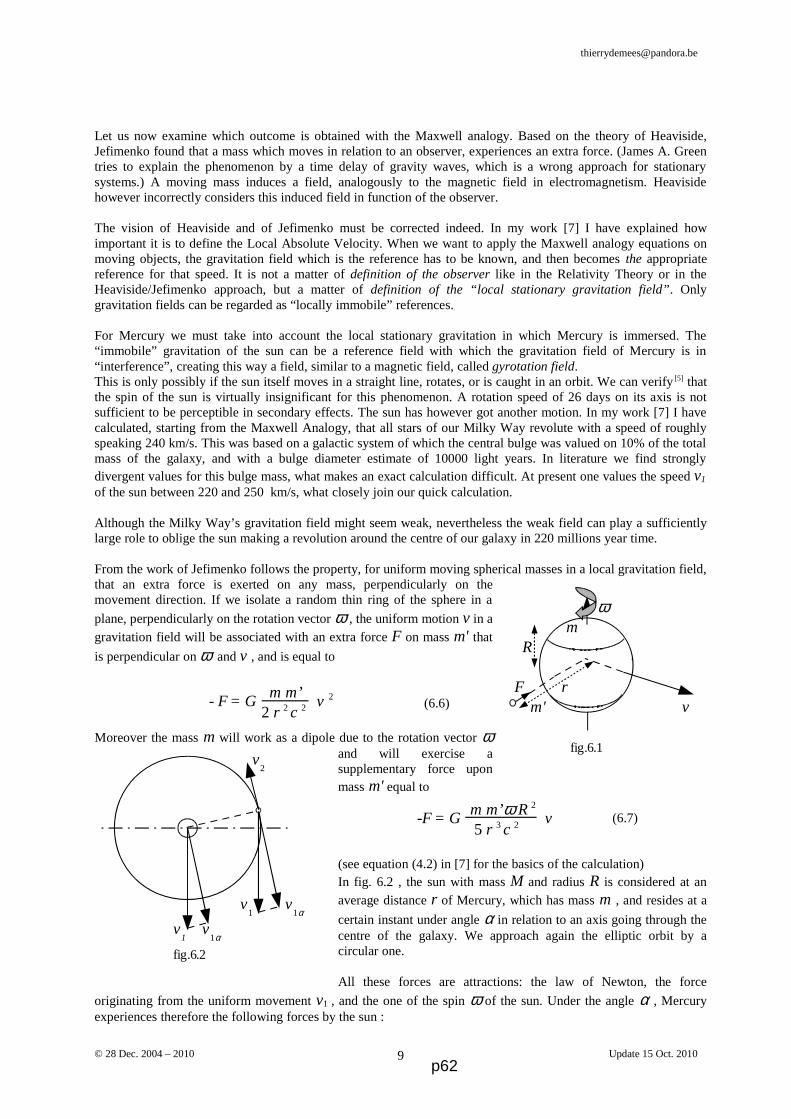
Let us now examine which outcome is obtained with the Maxwell analogy. Based on the theory of Heaviside,Jefimenko found that a mass which moves in relation to an observer, experiences an extra force. (James A. Greentries to explain the phenomenon by a time delay of gravity waves, which is a wrong approach for stationarysystems.) A moving mass induces a field, analogously to the magnetic field in electromagnetism. Heavisidehowever incorrectly considers this induced field in function of the observer.
The vision of Heaviside and of Jefimenko must be corrected indeed. In my work [7] I have explained howimportant it is to define the Local Absolute Velocity. When we want to apply the Maxwell analogy equations onmoving objects, the gravitation field which is the reference has to be known, and then becomes the appropriatereference for that speed. It is not a matter of definition of the observer like in the Relativity Theory or in theHeaviside/Jefimenko approach, but a matter of definition of the “local stationary gravitation field” . Onlygravitation fields can be regarded as “locally immobile” references.
For Mercury we must take into account the local stationary gravitation in which Mercury is immersed. The“immobile” gravitation of the sun can be a reference field with which the gravitation field of Mercury is in“interference”, creating this way a field, similar to a magnetic field, called gyrotation field. This is only possibly if the sun itself moves in a straight line, rotates, or is caught in an orbit. We can verify[5] thatthe spin of the sun is virtually insignificant for this phenomenon. A rotation speed of 26 days on its axis is notsufficient to be perceptible in secondary effects. The sun has however got another motion. In my work [7] I havecalculated, starting from the Maxwell Analogy, that all stars of our Milky Way revolute with a speed of roughlyspeaking 240 km/s. This was based on a galactic system of which the central bulge was valued on 10% of the totalmass of the galaxy, and with a bulge diameter estimate of 10000 light years. In literature we find stronglydivergent values for this bulge mass, what makes an exact calculation difficult. At present one values the speed v1
of the sun between 220 and 250 km/s, what closely join our quick calculation.
Although the Milky Way’s gravitation field might seem weak, nevertheless the weak field can play a sufficientlylarge role to oblige the sun making a revolution around the centre of our galaxy in 220 millions year time.
From the work of Jefimenko follows the property, for uniform moving spherical masses in a local gravitation field,that an extra force is exerted on any mass, perpendicularly on themovement direction. If we isolate a random thin ring of the sphere in a
plane, perpendicularly on the rotation vector ω , the uniform motion v in agravitation field will be associated with an extra force F on mass m' that
is perpendicular on ω and v , and is equal to
(6.6)
Moreover the mass m will work as a dipole due to the rotation vector ωand will exercise asupplementary force uponmass m' equal to
(6.7)
(see equation (4.2) in [7] for the basics of the calculation)In fig. 6.2 , the sun with mass M and radius R is considered at anaverage distance r of Mercury, which has mass m , and resides at a
certain instant under angle α in relation to an axis going through thecentre of the galaxy. We approach again the elliptic orbit by acircular one.
All these forces are attractions: the law of Newton, the force
originating from the uniform movement v1 , and the one of the spin ω of the sun. Under the angle α , Mercuryexperiences therefore the following forces by the sun :
© 28 Dec. 2004 – 2010 Update 15 Oct. 20109
ω m
R
F r m' v
fig.6.1
- F = G v 2 m m’
2 r 2 c 2
-F = G v m m’ω R 2
5 r 3 c 2
v2
M m αr
v1 v
1α
v1 v
1α
fig.6.2
p62
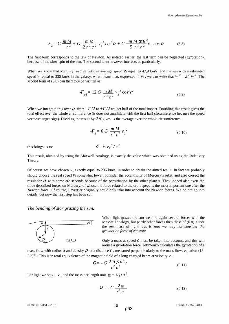
(6.8)
The first term corresponds to the law of Newton. As noticed earlier, the last term can be neglected (gyrotation),because of the slow spin of the sun. The second term however interests us particularly.
When we know that Mercury revolve with an average speed v2 equal to 47,9 km/s, and the sun with a estimatedspeed v1 equal to 235 km/s in the galaxy, what means that, expressed in v2 , we can write that v1
2 = 24 v2 2. The
second term of (6.8) can therefore be written as:
(6.9)
When we integrate this over α from –π /2 to +π /2 we get half of the total impact. Doubling this result gives thetotal effect over the whole circumference (it does not annihilate with the first half circumference because the speed
vector changes sign). Dividing the result by 2π gives us the average over the whole circumference :
(6.10)
this brings us to: δ = 6 v2 2 / c 2
This result, obtained by using the Maxwell Analogy, is exactly the value which was obtained using the RelativityTheory.
Of course we have chosen v1 exactly equal to 235 km/s, in order to obtain the aimed result. In fact we probablyshould choose the real speed v1 somewhat lower, consider the eccentricity of Mercury’s orbit, and also correct the
result for δ with some arc seconds because of the perturbation by the other planets. They indeed also exert thethree described forces on Mercury, of whose the force related to the orbit speed is the most important one after theNewton force. Of course, Leverrier originally could only take into account the Newton forces. We do not go intodetails, but now the first step has been set.
The bending of star grazing the sun.
When light grazes the sun we find again several forces with theMaxwell analogy, but partly other forces then these of (6.8). Sincethe rest mass of light rays is zero we may not consider thegravitation force of Newton!
Only a mass at speed c must be taken into account, and this willarouse a gyrotation force. Jefimenko calculates the gyrotation of a
mass flow with radius a and density ρ at a distance r , measured perpendicularly to the mass flow, equation (13-
2.2)[6] . This is in total equivalence of the magnetic field of a long charged beam at velocity v :
(6.11)
For light we set c=v , and the mass per length unit m = π ρ a 2.
(6.12)
© 28 Dec. 2004 – 2010 Update 15 Oct. 201010
m M m M m M ω R 2
r 2 2 r 2 c 2 5 r 3 c 2 -F
α = G + G v
1
2 cos2α + G v1 cos α
-Fα2
= 12 G v2
2 cos2αm M r 2 c 2
-F2 = 6 G v
2
2m M r 2 c 2
Ω = - G v2 π ρ a 2
r 2 c 2
Ω = - G 2 m
r 2 c
θ ∆ r
Rz fig.6.3
p63

Using (2.1) in which we set g=0 , we find the force per length unit :
(6.13)
Of course its validity remains for each length of the light ray.
The force caused by speed v1 , actually the orbit revolution speed of the sun in our galaxy, is given by the secondterm in (6.8). The angle φ is the angle between the light beam and the Milky Way's equator.
As last force we get the one of (6.7), whereof the size depends on the spin of the sun, and of course of the latitude
ϕ along which the light ray passes. The sun has actually a differential spin which varies according to the latitude:the poles rotate 30% more slowly than the equator. If we assume that, with respect to the sun, the speed of the
passing star light is the constant c, one may not take into account the speed v1 cos α of fig.6.2. in this term.
The last term of (6.14) comes from (6.7) where R = r and v = c . The angle θ is the angle between the lightbeam and the sun's equator.
The total force becomes this way:
(6.14)
The bending of light over the poles is therefore exactly the double of the calculation according to Newton, asexpected, but moreover there is an extra bending according to the position of the earth relative to the sun and to theMilky Way, and an extra bending which varies according to the latitude on the sun along which the light raypasses. The last term is positive (attraction bending) at the left side of the sun and negative (repulsion bending) atits right side, because of the spin direction of the sun.
7. Has the Relativity Theory era been fertile so far?
Nearly a century ago, one of two competitive theories has been put aside: the exact theory had to run off for theprofit of the wrong one! How could this come up to that point?Three elements to which the theory had to satisfy were known: the Newton limit, the bending of light and theprogress of Mercury’s perihelion. And moreover the theory had to offer a solution for the paradox of the Lorentzinvariance. To this invariance was even given a physical dimension (Lorentz contraction) subsequently to the testof Michelson-Morley.
The Relativity Theory was able to bring together all those elements to an apparently correct theory. Very certainlyalso Einstein must have known that with the Maxwell Analogy, the progress of Mercury’s perihelion could not beexplained. This for the simple reason that almost nothing was yet revealed of our galaxy. And on the other hand,the step to the Relativity Principle became still more easy because of the (wrong) principle of Heaviside that theobserver, and not the gravitation field, had to be seen as the reference for all calculations.
Thus, Einstein’s Relativity Theory arose, where all parameters were united, and which was moreover poured in aform that virtually deleted all tracks of the Maxwell Analogy: a curved space with an adapted kind of maths.
But something was nevertheless overlooked: the speed of light that is obtained by confronting in a certain way theAnalogue Maxwell Theory and the Relativity Theory is wrong. That ultimate discovery makes fail the RelativityTheory.
© 28 Dec. 2004 – 2010 Update 15 Oct. 201011
FΩ = - G 2 m Μ
r 2
-Fϕ,α,φ,θ
= G + G v1
2 cos2α cos2φ + G cosϕ cosθ2m M m M m M ωϕ r 2 2 r 2 c 2 5 r c
p64

However, it is astonishing that that discovery of James A. Green, as well as the many publications of other non-conventional scientists, seemingly are ignored by the proponents of the Relativity Theory, who constitute theestablishment. Why would this be this way? First, the theory has been expressed in a very concise way as adifferential equation. It is also very general, and after the appropriate calibration it allows each mathematicallycorrect solution as a possible real situation, even if it has not yet been discovered with our observation instruments.This frees the path in a fabulous way for predictions, what is of capital importance for science. The main reasonfor ignoring the Maxwell Analogy is probably also that on world scale, a complete army of scientists has beenproliferated out of the “Relativistic schools”, almost such as new religions ever arose and developed. Onceextended they are replaceable with difficulty.
Shortly after the First World War yet important solutions have been calculated with the theory.For instance, non-rotating black holes and wormholes were predicted long before there was any indication of theirexistence. Now one admits their existence, although non-rotating black holes have never been found yet, norwormholes. However, rotating black holes were observed meanwhile, which are not described by the theory,unless by introducing an extension of it.
In that sense the Relativity Theory has enormously contributed by being its time far ahead. It also showed theuniverse in an original and new manner: a curved universe, where nor the time, nor the distance, nor the mass haveabsolute values, but are different for each observer, and moreover it would be no illusion but be also like that inreality. Also cosmology progressed, by thoughts concerning the shape and the (in)finity of the universe.
But over the course of time this conduct is becoming a handicap for the Relativity Theory: calculations become thelonger the more complex. And it is uncertain that space is really curved, that mass and time really increase thatway with the speed, and that lengths really reduce that way. Oleg Jefimenko, James A. Green, and many othersdemonstrate adequately that also by means of the traditional physics all phenomena, and much more, can beexplained. How could it possible be else after what we discovered here!
We saw already some facts which Jefimenko and Green have demonstrated. Jefimenko also illustrated the affinitybetween both theories, and extended the Maxwell Analogy for not-static and non-linear cases. Green showed bymeans of the traditional working method, with the Maxwell equations, several phenomena at atomic scale. Idemonstrated in [7] that the speed of stars in disc galaxies satisfies the laws of Kepler, and that dark mass is amyth. Furthermore, why some rapidly rotating stars cannot burst entirely, why the mass expels of supernova andmust adopt stipulated profiles. The tore-like shape of rotating black holes was uncovered and was furtherdiscussed, and the reason for the many tiny Saturn rings proved in “Cassini-Huygens Mission”[8].
8. Conclusion: Did Einstein cheat?
We proved the validity of both the progress of the perihelion of Mercury and of the bending of light close the sunwith the Maxwell Analogy. Now the question remains open: did Einstein know that he made an error by definingits theory? Did Einstein cheat? A posteriori it seems indeed strange that Einstein succeeded, seemingly withoutmuch magic, to write down some simple looking equations, though by means of a strange and complicated type ofmaths for that time, and moreover little common.
On the other hand Einstein must have known that the Mercury problem was not soluble by means of the MaxwellAnalogy with the observations and the measuring known at that time. An appropriate calibration of the RelativityTheory therefore has been done (Einstein's field equations are indeed deducted from the equation -named Einstein-Hilbert action- for a "space", extended with the equation -named Lagrangian- for the definition of mass in that
space. Also Einstein defined a required factor k as k -1 = 16 π G c -4. Finally, Cartan extended the theory forrotating objects.) It is at last between 1911 and 1914 that Einstein must have known that the bending of lightgrazing the sun rather had the double value of the one according to Newton. Did Einstein intuitively fall on thegood looking equations at that period? Was the new type of maths necessary to increase the detachment to theMaxwell Analogy and to conceal the calibrations?
Probably we should not judge Einstein too quickly. Although it might be possible that, thanks to somecalculations, Einstein got on that “good” track in a converging manner, consciously cheating is still another thing.
© 28 Dec. 2004 – 2010 Update 15 Oct. 201012 p65

The main reasons for the new track which Einstein made was the need to incorporate the contraction of length(and thus of time) as a part of the theory, and the impossibility of building further on the Maxwell Analogybecause of the Mercury problem. The glory that the theory of Einstein obtained was, among others, thanks to thesudden revelation, after more than ten years of inventively and intuitively work, of a theory in a mathematicallynew appearance, original and general, and one which made extrapolations to cosmology possible.And we can expect that both competitive theories will still continue existing in parallel, possibly for decades.
9. References and interesting literature.
1. Einstein, A., 1916, Über die spezielle und die allgemeine Relativitätstheorie.
2. Feynman, Leighton, Sands, 1963, Feynman Lectures on Physics Vol 2.
3. Green, J. A., 2002, Gravitation & the Electroform Model: From General Relativity to Unified Field Theory.
4. Heaviside, O., A gravitational and electromagnetic Analogy, Part I, The Electrician, 31, 281-282 (1893)
5. Jefimenko, O., 1991, Causality, Electromagnetic Induction, and Gravitation, (Electret Scientific , 2000).
6. Jefimenko, O., 2006, Gravitation and Cogravitation, (Electret Scientific , 2006).
7. De Mees, T., 2003, A coherent double vector field theory for Gravitation.
8. De Mees, T., 2004, Cassini-Huygens Mission.
9. www.maths.com
© 28 Dec. 2004 – 2010 Update 15 Oct. 201013 p66
Thierry De Mees
On the Origin of the Lifetime Dilatation of High Velocity Mesons
Described by using Gravitomagnetism.
T. De Mees - thierrydemees @ pandora.be
Abstract
We analyze here the influence of gravitomagnetism upon fast moving particles and we find a physical mechanismfor the lifetime dilation of mesons at very high velocities. One of the later arguments in favor of the SpecialRelativity Theory (SRT) was the discovery of a lifetime dilation of high velocity mesons. However, it has alsobeen found that the observed lifetime dilation didn't correspond to SRT predictions. Moreover, SRT neitherGeneral Relativity Theory (GRT) ever explained any physical mechanism. When using gravitomagnetism, itbecomes clear that not a time delay, but an self-inductive gravitomagnetic compression component is responsiblefor a delayed decay of the meson. We also find that relativistic mass doesn't exist, but that only the gravitationalfield gets accumulated to high values when the object's speed is close to the speed of light.
Key words : gravitation, gravitomagnetism, gyrotation, meson lifetime, Heaviside, Maxwell analogy.Method : analytical.
1. Pro memore : The Heaviside (Maxwell) Analogy for gravitation (or gravitomagnetism).
Heaviside O., 1893, transposed the Electromagnetism equations of Maxwell into the Gravitation of Newton,creating so a dual field : gravitation and what we propose to call gyrotation (which is the gravitational equivalenceof magnetism), where the last field is nothing more than an additional field caused by the velocity of theconsidered object against the existing gravitation fields.
The formulas (1.1) to (1.5) form a coherent set of equations, similar to the Maxwell equations[1]. Electrical chargeis then substituted by mass, magnetic field by gyrotation, and the respective constants as well are substituted (the
gravitation acceleration is written as g , the “gyrotation field” as Ω Ω Ω Ω , and the universal gravitation constant G as
G-1 = 4π ζ ). We use sign ⇐ instead of = because the right hand of the equation induces the left hand. This signwill be used when we want to insist on the induction property in the equation.
F ⇐ m (g + v × Ω Ω Ω Ω ) (1.1)
∇∇∇∇ . g ⇐ ρ / ζ (1.2)
c²∇∇∇∇× ΩΩΩΩ ⇐ j / ζ + ∂ g /∂ t (1.3)
where j is the flow of mass through a surface.
It is also expected :
div ΩΩΩΩ ≡ ∇ ∇ ∇ ∇.ΩΩΩΩ = 0 (1.4)
∇∇∇∇×g ⇐ - ∂ ΩΩΩΩ / ∂ t (1.5)
and c2 = 1 / ( ζ τ ) (1.6)
wherein τ = 4π G/c2
All applications of the electromagnetism can from then on be applied on the gravitatiomagnetism with caution.
© 2010 release 26 February 20101 p67

Thierry De Mees
2. Gravitomagnetic induction.
2.1. Gyrotational induction and Lorentz-like force for gravitation.
A particle “A” travels at high velocity nearby the Earth. It lays in the Earth'sgravitational field and creates a gravitomagnetic field (the gyrotation field) thatis circular about its body.
Another mass “B” at high speed and with a path that is here parallel to “A” canbecome influenced by that gravitomagnetic field (the gyrotation).
It then undergoes a Lorentz-like force[1] that make the masses undergo anadditional attraction force given by
This Lorentz-like force works as follows: both masses feel the other magneticfield, that generates a force F upon the particle.
The gyrotational force is given by : F ⇐ mB (v × Ω Ω Ω Ω ) (2.1)
and the gyrotation field ΩΩΩΩ is found by[1]:
(2.2)
which is a transcription of (1.3) into integrals, valid for constant values of the gravitation field g.
The equation (2.1) can in this case simply be written as ΩΩΩΩ ⇐ 2 G v dmA/(dy r c2) because ΩΩΩΩ is constant
over each circular path 2π r . Herein r is the distance between the masses mA and mB , r = |A – B| . The
distance dy is the infinitesimal length of particle A along the y–axis for this process.
The combination of the equations (2.1) and (2.2) gives then for a local place y :
dF/dy ⇐ 2 G dmA/dy . dm
B/dy . v2/(r c2) (2.3)
This kind of gravitomagnetic induction happens between the Sun and the planets and is responsible for the flatnessof our solar system. It also explains the flatness of disc galaxies and the constancy of the star's velocity in discgalaxies without any need for “dark mass”. See also section 2.3 for further explanations.
2.2. Gyrotational self-induction of rectilinear fast particles and its global cylindrical pressure.
A mass that travel in a gravitation field creates a magnetic-like field, called gyrotation field, as shown in fig. 2.1.This field is circular and it is also present inside and at the surface of the object. The global gyrotation field is
produced by the sum of all the particles of the object, but that field also actson each single particle of that object. This really means that each of theparticles undergo a Lorentz-like force that is perpendicular on both the paththat the object follows and the gyrotation field (see fig. 2.2).In other words, there is a Lorentz-like force that compresses the objectcylindrically over the whole object and that helps the object not to disintegrateat high velocities.
The gyrotational acceleration is given by :
a = dF/dm ⇐ (v × Ω Ω Ω Ω ) (2.4)
© 2010 release 26 February 20102
z
Ω v y
x'
Ω
v y
x
A
B
FF
Fig. 2.1 : two particles attract due to their velocity.
∫ ΩΩΩΩ . dl ⇐ 4π G mA / c2.
Fig. 2.2 : a particle is compressed due to its velocity.
v y
F Ω
r
p68

Thierry De Mees
and the gyrotation field ΩΩΩΩ is found by:
(2.5)
which is a transcription of (1.3) into integrals, valid for constant values of the gravitation field g.
The equation (2.5) can in this case simply be written as ΩΩΩΩ ⇐ 2 G v dm/(dy r c2) because ΩΩΩΩ is constant
over each circular path 2π r . Herein r is the variable diameter of the cross section of mass m on the place y . Thedistance dy is the infinitesimal length of the mass along the y–axis for this process.
The combination of the equations (2.4) and (2.5) gives then at a place r of the mass the acceleration (compression)a(r) :
a(r) = dF/dm ⇐ 2 G dm/dy . v2/(r c2) (2.6)
The local pressure p(r) at the variable place r is then given by :
p(r) = dF/dA ⇐ G (dm/dy)2 . v2/(π r2 c2) (2.7)
For a sphere with density ρ : p(r) ⇐ π G r2ρ v2/c2 = 3 G m v2/(4 r c2
) (2.8)
The equation (2.8) is valid for not too fast particles because it didn't take in account the time delay of thegravitation field between the object's mass and its surface. Let us see below what this means.
2.3. How does a high speed gravitation field look like?
Oleg Jefimenko proved that the velocity increase of a particle results in the flattening of the gravitationalspectrum. This flattens the gravitational field, perpendicularly to the path of motion. The gravitational zones in thedirection of the motion of the particle, are decreasing with the velocity.
The original equation of Oliver Heaviside that he wrote down atthe end of the 19th century showed already the dependency of
the angle θ (see fig. 2.3) with the retarded value of thegravitation field for a fast moving mass.
(2.9)
Equation (2.9) gives the value of the local gravitation for a certain mass m at a velocity v. Thus, for very highspeeds, we have put equation (2.5) in a more general form, as follows :
(2.10)
In fact, (2.10) is physically speaking more correct than (2.5) because not the mass, but the interaction betweenmoving gravitation fields is responsible for the creation of the gyrotation field.By using (2.9) we can easily recalculate equation (2.8) in the case of a sphere:
(2.11)
© 2010 release 26 February 20103
∫ ΩΩΩΩ . dl ⇐ 4π G m / c2.
Fig. 2.3 : a particle's gravitation field is heterogeneous due to its velocity.
g r Gm v c
r v c,
sinθ
θb g c h
c he j=
−
−
1
1
2 2
2 2 2 23 2
gv
θr
∫ ΩΩΩΩ . dl ⇐ 4π G g r2 / c2.
p rg v rc
G m v v c
r c v c,
sinθ
θb g c h
c he j⇐ =
−
−
3
4
3 1
4 1
2
2
2 2 2
2 2 2 23 2
p69

Thierry De Mees
On top of that, we also should include a retardation of the field along the path of the object. The object will befurther than its gravitation or gyrotation field would suggest.
2.3. Gyrotational self-induction of rectilinear very fast particles and its delayed global cylindrical pressure.
For very high speeds, such as cosmic mesons, reaching nearly the speed of light, the compression at the place r ,assuming the meson as a homogeneous sphere, is given by (2.11) where the divider of the quotient becomes close
to zero, especially for angles nearby π/2. Due to the global exponent of -1/2 ,
the pressure becomes close to infinite. Away from π/2 , the pressure becomesrapidly very low.
This signifies that the gravitational field can end up to become infinite at π/2when the velocity of light is reached.The meson is compressed by a very high cylindrical pressure all around it, thathinders the meson from decaying, unless the velocity has been reduced tolower values.Besides, due to the position of the delayed fields, behind the meson'sprogression path, the compression will be somewhat conical instead ofcylindrical, making the decay more difficult at the back side of theprogression path. Due to the high speed, the decay can not occur ahead of the
progression path either, because that would require an even higher velocity of the decay residues.
This proves that the lifetime delay of the meson is physically made possible by a compression rather than a changeof the time dimension.
3. Discussion and conclusion: does relativistic mass exist?
When a particle in the CERN accelerator is accelerated, magnetic fields are used. These magnetic fields can only“push” the particles at not more than the speed of light. Moreover, the magnetic fields are put under an angle tothe particle's path. Thus, the particles never can reach the speed of light because the magnetic fields, under anangle to the particles' path, are always themselves below the speed of light. And just as in equation (2.9) for gravitomagnetism, charged particles in CERN never can be accelerated by
magnetic fields up to the speed of light because of the quasi fully π/2–orientation of the electrical field at thatspeed.
But does that mean that the particle's mass is increasing by velocity? No, it isn't. The consequence of a highvelocity is the self-inductive cylindrical compression upon the particles, as explained above. Relativistic massdoesn't exist.We can show this by the following. Equation (2.9) shows that not the mass but the gravitation field is locally
increasing, especially for the angle around π/2. But can the global value of g in equation (2.9) reach infinity at speeds that are close to the speed of light?
To know that, the easiest way is to argue as follows: if we consider the highest value for (2.9) by putting sinθ = 1,we get :
(3.4)
and this confirms that at the speed of light, the global gravitation field is theoretically able to reach infinity, due tothe accumulation of the gravitation waves at that speed, the same as what happens with the sound waves of aplane, just before it passes the sound barrier.
© 2010 release 26 February 20104
v y
F
Ω
r
Fig. 2.4 : a particle's gyrotation field and therefore its compression is heterogeneous due to its velocity.
g rG m
r v c, dθ θ ππ
b g0
2
2 2 22 1z ≤
−
p70

Thierry De Mees
Remember however that the direction of that infinite gravitational field is oriented at the angle of θ = π/2 andthat at other angles (thus all other directions), the gravitation field is decreasing quickly !
4. References and interesting literature.
1. De Mees, T., 2003, A coherent double vector field theory for Gravitation.
2. De Mees, T., 2004, Did Einstein cheat ?
3. Feynman, Leighton, Sands, 1963, Feynman Lectures on Physics Vol 2.
4. Heaviside, O., A gravitational and electromagnetic Analogy, Part I, The Electrician, 31, 281-282 (1893)
5. Jefimenko, O., 1991, Causality, Electromagnetic Induction, and Gravitation, (Electret Scientific, 2000).
© 2010 release 26 February 20105 p71
© 2005 Thierry De Mees
1
On the geometry of rotary stars and black holes
T. De Mees - [email protected]
Abstract
Encouraged by the great number of explained cosmic phenomena by using the Maxwell Analogy for Gravitation(7,8,9) (or the “Heaviside field”) instead of the General Relativity Theory, we study closer the fast rotary stars that we have studied earlier(7). We find the detailed reason for the double-lobes explosions of supernova, and for the equator explosions. A part of the star is insensible to fast rotation, and at the contrary is more attracting the faster it spins. We find for spherical stars important velocity-independent angles, defining partly their final torus-like shape. We found this by recognizing that moving masses generate a second field, analogue to magnetism, that we call gyrotation(7). Keywords. Maxwell analogy – gravitation – star: rotary – black hole – torus – gyrotation – methods : analytical Photographs : ESA / NASA Index 1. Introduction : the Maxwell analogy for gravitation, summarized.
2. Gyrotation of spherical rotating bodies in a gravitational field.
3. Explosion-free zones and general shape of fast spinning stars.
The Critical Compression Radius for Rotary Spheres
Surface compression of fast rotating stars.
The internal compression acceleration by gyrotation
The equatorial explosion area
The shape of fast rotating stars
Validation of the theory
4. General remnants’ shape of exploded fast spinning stars.
Spherical spinning stars
Spinning black hole torus
5. Conclusions.
6. References.
p72

Thierry De Mees - Leeuwerikenlei 23 - 2650 Edegem [email protected]
Jul. 2005 release 30/07/2005 2
The first and second chapter are summaries of chapters 1 to 4 of reference 7. 1. Introduction : the Maxwell analogy for gravitation, summarized.
The Maxwell Analogy for gravitation can be put in the compact equations, given by Heaviside(4). The formulas (1.1) to (1.5) form a coherent set of equations, similar to the Maxwell equations. Electrical charge is then substituted by mass, magnetic field by gyrotation, and the respective constants as well are substituted (the gravitation acceleration is written as g , the so-called “gyrotation field” as Ω Ω Ω Ω, and the universal gravitation constant as G = (4π ζ)-1. We use sign ⇐ instead of = because the right hand of the equation induces the left hand. This sign ⇐ will be used when we want to insist on the induction property in the equation. F is the induced force, v the velocity of mass m with density ρ. Operator × is used as a cross product of vectors. Vectors are written in bold.
F ⇐ m (g + v × ΩΩΩΩ) (1.1)
∇∇∇∇ g ⇐ ρ / ζ (1.2)
(1.3) where j is the flow of mass through a surface. The term ∂g/∂t is added for the same reasons as Maxwell did: the compliance of the formula (1.3) with the equation It is also expected div ΩΩΩΩ ≡ ∇ ∇ ∇ ∇ ΩΩΩΩ = 0 (1.4)
and ∇∇∇∇× g ⇐ – ∂ ΩΩΩΩ / ∂ t (1.5)
All applications of the electromagnetism can from then on be applied on gravitomagnetism with caution. Also it is possible to speak of gravitomagnetism waves. 2. Gyrotation of spherical rotating bodies in a gravitational field.
For a spinning sphere, the results for gyrotation are given by equations inside the sphere (2.1) and outside the sphere (2.2):
(2.1) (2.2) fig. 2.1
(Reference: adapted from Eugen Negut, www.freephysics.org) The drawing shows equipotentials of – Ω . wherein • means the scalar product of vectors. For homogeny rigid masses we can write :
(2.3)
div j ⇐ – ∂ρ / ∂ t
– 4 π G ρ 2 1 r (r • ωωωω) c2 5 3 5
ΩΩΩΩint ⇐ ωωωω ( r2 – R2) – ωωωω Y p r α X R
ΩΩΩΩext ⇐ ωωωω – – G m R2 3 r (ω ω ω ω • r) 5 r3 c2 r2
ΩΩΩΩext ⇐ – – 4 π G ρ R5 ω ω ω ω r (ω ω ω ω • r) 5 r3 c2 3 r2
c² ∇∇∇∇× ΩΩΩΩ ⇐ j / ζ + ∂g /∂ t
p73
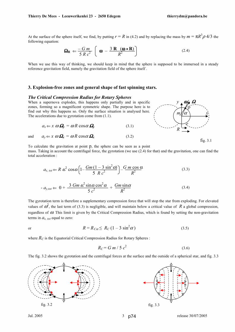
Thierry De Mees - Leeuwerikenlei 23 - 2650 Edegem [email protected]
Jul. 2005 release 30/07/2005 3
At the surface of the sphere itself, we find, by putting r = R in (4.2) and by replacing the mass by m = πR3ρ 4/3 the following equation:
(2.4) When we use this way of thinking, we should keep in mind that the sphere is supposed to be immersed in a steady reference gravitation field, namely the gravitation field of the sphere itself . 3. Explosion-free zones and general shape of fast spinning stars. The Critical Compression Radius for Rotary Spheres When a supernova explodes, this happens only partially and in specific zones, forming so a magnificent symmetric shape. The purpose here is to find out why this happens so. Only the surface situation is analysed here. The accelerations due to gyrotation come from (1.1).
ax ⇐ x ω ΩΩΩΩy = ω R cosα ΩΩΩΩy (3.1) and ay ⇐ x ω ΩΩΩΩx = ω R cosα Ω Ω Ω Ωx (3.2) To calculate the gravitation at point p, the sphere can be seen as a point mass. Taking in account the centrifugal force, the gyrotation (we use (2.4) for that) and the gravitation, one can find the total acceleration :
(3.3)
(3.4) The gyrotation term is therefore a supplementary compression force that will stop the star from exploding. For elevated values of ω2, the last term of (3.3) is negligible, and will maintain below a critical value of R a global compression, regardless of ω. This limit is given by the Critical Compression Radius, which is found by setting the non-gravitation terms in ax, tot equal to zero:
or R = RC α ≤ RC (1 – 3 sin2α ) (3.5)
where RC is the Equatorial Critical Compression Radius for Rotary Spheres :
RC = G m / 5 c2 (3.6)
The fig. 3.2 shows the gyrotation and the centrifugal forces at the surface and the outside of a spherical star, and fig. 3.3
y ω Ωω Ωω Ωω Ω p
m α x
r R
fig. 3.1
fig. 3.2 fig. 3.3
– G m 3 R (ω ω ω ω • R) 5 R c2 R2
Ω Ω Ω ΩR ⇐ ωωωω –
- ay,tot ⇐ 0 + + 3 Gm ω2 sin α cos2α Gm sinα 5 c2 R2
ax, tot ⇐ R ω2 cos α 1– – Gm (1 – 3 sin2 α) G m cos α
5 R c2 R2
p74

Thierry De Mees - Leeuwerikenlei 23 - 2650 Edegem [email protected]
Jul. 2005 release 30/07/2005 4
shows the gyrotation lines and forces at the inner side of the star. This can be found with (2.1) and (2.2). Surface compression of fast rotating stars. For spheres with R ≤ RC , a global surface compression takes place for each angle α wherefore –αC < α < αC , and wherefore
αC = arc sin (3-1/2 (1– R/RC)1/2) (3.7) Remark that always αC ≤ 35°16’, and it’s value depends from the sphere’s radius. Hence, explosions are exclusively expected under –αC and above αC .
In fig.3.4 , the graph shows the relationship (3.7) between R/RC and αC for ax, tot = 0 (we disregard the gravitation acceleration). When R/RC = 1, only the equator is potentially protected against explosion. The smaller R, the larger the protection area (–αC ≤ α ≤ αC) is where global compression occur.
Another view is given in fig.3.5.a , where the spin-dependent factor of ax, tot /(R ω2) in (3.3), by using (3.6) and by setting x =α° , has been calculated for several values of R/RC (respectively 1, ½ , ¼ ,…, 1/32). Compression occur when the values are negative. We conclude that the smaller R/RC , the wider the compression-area becomes.
fig.3.4.
fig. 3.5.a
p75
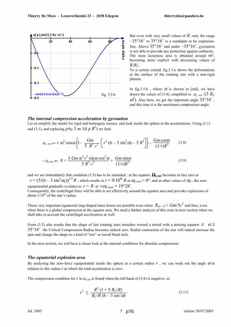
Thierry De Mees - Leeuwerikenlei 23 - 2650 Edegem [email protected]
Jul. 2005 release 30/07/2005 5
But even with very small values of R, only the range –35°16’ to 35°16’ is a candidate to be explosion-free. Above 35°16’ and under –35°16’, gyrotation is not able to provide any protection against outbursts. The most looseness area is obtained around 60°, becoming more explicit with decreasing values of R/RC . To a certain extend, fig.3.5.a shows the deformations at the surface of the rotating star with a non-rigid plasma. In fig.3.5.b , where α is shown in [rad], we have drawn the values of (3.4), simplified to ay, tot /(3 RC ω2). Also here, we get the important angle 35°16’ , and this time it is the maximum compression angle.
The internal compression acceleration by gyrotation Let us simplify the model for rigid and homogeny masses, and look inside the sphere at the accelerations. Using (2.1) and (3.1), and replacing ρ by 3 m /(4 p R3) we find:
(3.8)
(3.9) and we see immediately that condition (3.5) has to be amended : at the equator, ΩΩΩΩy,int becomes in fact zero at r = (5/(6 – 3 sin2αE))1/2 R , which results in r = 9/10th R at αE,min = 0°, and at other values of αE , the zero equipotential gradually evolutes to r = R at ±αE,max = 19°28’. Consequently, the centrifugal force will be able to act effectively around the equator area and provoke explosions of about 1/10th of the star’s radius. These very important equatorial ring-shaped mass losses are possible even when Rα = 0 < Gm/5c2 and thus, even when there is a global compression at the equator area. We need a further analysis of this zone in next section when we shall take in account the centrifugal acceleration as well. From (3.5) also results that the shape of fast rotating stars stretches toward a toroid with a missing equator: if α ≥ 35°16’ the Critical Compression Radius becomes indeed zero. Radial contraction of the star will indeed increase the spin and change the shape to a kind of “tire” or toroid black hole. In the next section, we will have a closer look at the internal conditions for absolute compression. The equatorial explosion area By analysing the zero-force equipotential inside the sphere at a certain radius r , we can work out the angle α in relation to this radius r at which the total acceleration is zero. The compression condition for r in ax,tot is found when the left hand of (3.8) is negative, or: (3.11)
R2 (1 + 5 RC/R) RC/R (6 – 3 sin2α)
r2 ≤
- ay,tot ⇐ 0 + + 3 Gm ω2 r3 sin α cos2α Gm sinα 5 R3 c2 (1/r)R3
Gm Gm cos α
5 R3 c2 (1/r)R3 ax, tot ⇐ r ω2 cosα 1– r2 (6 – 3 sin2α) – 5 R2 –
fig. 3.5.b
p76

Thierry De Mees - Leeuwerikenlei 23 - 2650 Edegem [email protected]
Jul. 2005 release 30/07/2005 6
In order to simplify, we have considered the gravitation force as being insignificant, which is true for fast rotating stars. In fig.3.6, we show the graph of (3.11) for R = ¾ RC , R = ½ RC , R = ¼ RC , and for very small R/RC. The boundary of the sphere is shown as well. The x-axis is α and the y-axis is r/R. In the case of R = ½ RC , only a very small region wherefore –17°43’ ≤ αN ≤17°43’ is affected by an explosion zone, based on the spherical intersection point with the explosion area. About 4% of the equator radius can be blown out. We call RN the remaining equatorial radius. And when we take the limit to very small values of R, the following graph is found: an explosion zone around the
equator of the sphere until about αN,max=25°27’ with a blow-out opportunity of 9% of the radius (fig.3.6). At this stage we are able to stress the global shape of fast rotating stars and to define the location of the possible outbursts. The shape of fast rotating stars Until now, we have found a number of criteria that are valid for fast rotating spheres:
1) When R ≤ RC , there exist a zone where no explosion can occur (considering gravitation as negligible). 2) The smaller R/RC , the bigger the zone between the equator and the maximal compression angle αC , where
no outbursts can occur. The maximal possible explosion-free zone is –35°16’ to 35°16’. 3) The equator is not explosion-free: when R ≤ RC , there exists a ring-shaped zone inside the sphere where an
explosion may occur, pushing an equator belt outwards. 4) The smaller R/RC , the larger the exploded zone around the equator, and the maximal explosion angle is about
±αN,max=25°27’, while about 9% of the equator can be blown out. 5) The area around 60° , having a top value (α , ax,tot) depending from R/RC , is the most looseness area.
The maximum compression area of ay,tot goes until ±α = 35°16’.
fig.3.6
12°25’
17°43’
21°56’
25°27’
αC ωωωω non-compression area αN,max
R
RN compression area
fig.3.7 : exploded rotary black hole
p77

Thierry De Mees - Leeuwerikenlei 23 - 2650 Edegem [email protected]
Jul. 2005 release 30/07/2005 7
Using these criteria, the general geometry of a fast rotating star can be drawn, and the exploded star can be defined in general lines. A torus, limited by the angle αC , beyond which no matter is present, and limited as well by the angle αN,max , which lays between αC and the equator. At the equator, the radius is restricted to RN ≤ R that can be found by setting α = 0 in (3.11) (see fig.3.7). The internal radius of the torus-like star is zero or almost zero after the explosion, according to the known criteria. Validation of the theory The theory can not yet be verified very precisely because the values of m, G, ω and R are not known for distant supernova and quasars. However, observation of exploding stars shows the presence of an explosion at the equator and one at a zone above a certain angle, measured from the equator. We claim the compliance between the theory and observation in its general aspect. In the next chapter however, we will see what happens with the remnants. When the matter explodes, the theory predicts that the star’s gyrotation obliges it to move in a prograde direction. The global
motion will be spirally outwards. Finding evidence by observation is difficult for this property as well, because a high astronomic precision is necessary. But in general lines, both observations agree perfectly with the theory with simple analytic calculus, which is a great improvement against the General Relativity Theory. 4. General remnants’ shape of exploded fast spinning stars. In the former chapter, we could see how the gravitation equations of spinning stars could explain their general geometry, and could define the explosion-free zones. In this chapter, we look more closely at the remnants. Spherical spinning stars. If a spinning sphere begins exploding, matter is leaving the surface tangentially. Gyrotation equipotentials are as shown in fig.4.1. The gyrotation acceleration will be oriented towards the equator and will generate a deviation of the matter in a widening prograde spiral. In the figure, fine dotted lines show the boundaries of the spirally escaping matter, which knock at the equator level. The plain line curved arrows are the paths of exploding matter.
ΩΩΩΩ
ΩΩΩΩ y x
fig. 3.9 SN 1987A η Carinae
SN 1987A: a local mass loss took place on the equator and at the angle αC . The zone near the poles exploded possibly much earlier, so it became a toroid-like shaped rotary star. η Carinae : mass loss by complete shells, above αC , forming two lobes with a central ring.
fig. 3.8
p78

Thierry De Mees - Leeuwerikenlei 23 - 2650 Edegem [email protected]
Jul. 2005 release 30/07/2005 8
The typical shape of such an explosion is shown in fig.4.2. The remnants are restricted to almost a cylinder. The equatorial region could possibly explode but not necessarily, depending on the rotation velocity. Besides, the star is not necessarily a black hole in order to get such a remnants shape. We clearly see two cylindrical lobes, with in the middle a huge spherical halo around the spherical star. At the equator level, a line is visible (here, under a slight angle with the equator), which splits the halo in two hemispheres. This is the contact plane of knocking remnants of the northern and the southern hemisphere.
Spinning black hole torus. The sphere explodes, and becomes hereafter a butterfly-shaped black hole torus.The gyrotation equipotentials of exploded black holes are expected to have a butterfly shape (fig.4.3, dotted lines). When new matter is blown out tangentially, and this happens above the limit αC (fig.4.3, curved plain line), the gyrotation acceleration will be oriented away from the equator, and deviate the matter in a widening prograde spiral, due to (1.1). In fig.4.3, we have represented a flattened sphere and two sections of the black hole torus.The black hole arose indeed after a strong reduction of the diameter of the original sphere and after a flattening of the poles in an ellipsoid shape, with a strong increase of the spinning velocity as a consequence. A typical example for these remnants is given by the supernova SN 1987A (fig.3.8), while η Carinae doesn’t show it as clearly, but has probably also gotten an identical process. 5. Conclusions. The Maxwell Analogy for Gravitation gives a clear picture of what we can expect as the conditions for a rotary black hole with non-exploding regions.
Fig. 4.2
ω Ωω Ωω Ωω Ω y
v m a ΩΩΩΩ x fig. 4.1
αC ω ω ω ω a vαN,max R
ΩΩΩΩ
RN
fig.4.3
p79

Thierry De Mees - Leeuwerikenlei 23 - 2650 Edegem [email protected]
Jul. 2005 release 30/07/2005 9
When R ≤ RC , there exist zones where no explosion can occur (if gravitation is negligible). The smaller R/RC , the larger the area between the equator and the maximal compression angle αC , where no outbursts can occur. The maximal possible explosion-free zone is –35°16’ to 35°16’. The equator is not explosion-free: when R ≤ RC , there exist a zone where an explosion may occur. The smaller R/RC , the larger the exploded zone around the equator, and the maximal explosion angle is about αN,max=20°, while about 9% of the equator can be blown out. The shape of fast spinning stars that did explode due to the spin velocity, ends-up to a torus-like black hole with a missing equator-zone. The remnants of spinning spheres will form two lobes of prograde spirally matter, but unlikely an equatorial explosion. At the other hand will the northern and the southern remnants knock at the equator level, and form a halo between the two lobes. For fast spinning black holes which exploded before, new burst-outs will form two lobes of prograde spirally matter, and will follow a path outwards, without passing over the equator. 6. References. 1. Einstein, A., 1916, Über die spezielle und die allgemeine Relativitätstheorie. 2. Feynman, Leighton, Sands, 1963, Feynman Lectures on Physics Vol 2. 3. Green, J. A., 2002, Gravitation & the Electroform Model: From General Relativity to Unified Field Theory.
4. Heaviside, O., A gravitational and electromagnetic Analogy, Part I, The Electrician, 31, 281-282 (1893)
5. Jefimenko, O., 1991, Causality, Electromagnetic Induction, and Gravitation, (Electret Scientific Cy, 2000).
6. Jefimenko, O., 1997, Electromagnetic Retardation and Theory of Relativity, (Electret Scientific Cy, 2004).
7. De Mees, T., 2003, A coherent double vector field theory for Gravitation.
8. De Mees, T., 2004, Cassini-Huygens Mission.
9. De Mees, T., 2004, Did Einstein cheat ?
10. Negut, E., On intrinsic properties of relativistic motions, 1990, Revue Roumaine des Sciences Techniques.
11. www.maths.com
p80
4The Behavior ofRotating Stars andBlack Holes
I wrote four papers up to now concerning fast spinning stars and black holes. WithGravitomagnetism, it appears that fast spinning stars are compressed at their surface in order to notexplode completely and to form hourglass supernovae (I called it “diabolo”, like the game with arope). This comes in the first paper.The Kepler-Newton orbital speeds about fast spinning stars are not respected but are faster, asexplained in the second paper. The reason therefore comes in the fourth paper : fast spinning starsand black holes have an apparent mass that is far above its real mass, due to their extra gyrotationforce.But another aspect about fast spinning stars and black holes is the event horizon issue. Thereappears to be two kind of event horizons, which act only on a part of the stars. Many black holes arenever totally black!Explore now the strange world of fast spinning stars!
p81
© 2006 Thierry De Mees
On the orbital velocities nearby rotary stars and black holes
T. De Mees - [email protected]
Abstract
Observation of some huge spinning black holes in the centre of galaxies, and surrounded by orbiting stars, shows that stars close-by the black hole orbit at much higher speeds than normally expected, whereas the velocity of stars at higher distances suddenly falls down to normal values.In a former paper “On the shape of rotary stars and black holes” I found the analytic expressions for the forces on rotary stars and black holes, due to the gyrotation forces. These forces are generated by the second field of gravitation, based on the Maxwell Analogy for Gravitation(5,6,7,8) (or historically more correctly: the Heaviside(2) Analogy for Gravitation). In earlier papers, I showed the great workability of this analytical method, at the condition that the “local absolute velocity” is defined in relation to a major gravitational field instead of the “observer system” as with GRT. I found so the detailed explanation for the double-lobes explosions of supernova, and for the equator explosions. Here, I deduct the velocity distribution of orbital objects nearby or farther away from rotary stars or black holes.
Keywords. Maxwell Analogy – gravitation – star: rotary – black hole – torus – gravitomagnetism – methods : analyticalPhotographs : ESA / NASA
Index
1. Introduction : the Maxwell analogy for gravitation.
2. Gyrotation of spherical rotating bodies in a gravitational field.
3. Orbital velocity nearby fast spinning stars.
Total orbital acceleration in the equatorial plane.
Total orbital velocity in the equatorial plane for spherical and toric fast spinning stars.
Discussion.
Validation of the calculus.
4. Conclusion.
5. References.
1 p82

© 2006 Thierry De Mees [email protected]
1. Introduction : the Maxwell analogy for gravitation (gravitomagnetism).
The Maxwell Analogy for gravitation can be put in compact equations, originally given by Heaviside(2, 3, 5). Electrical charge is then substituted by mass, magnetic field by gyrotation, and the respective constants as well are substituted (the gravitation acceleration is written as g , the so-called “gyrotation field” as Ω, and the universal gravitation constant as G = (4π ζ)-1. I use sign ⇐ instead of = because the right hand of the equation induces the left hand. This sign ⇐ will be used when we want to insist on the induction property in the equation. F is the induced force, v the velocity of mass m with density ρ. Operator × is used as a cross product of vectors. Vectors are written in bold.All applications of the electromagnetism can from then on be applied on gravitomagnetism with caution. Also it is possible to speak of gravitomagnetism waves. Please read my earlier papers for a better comprehension(5, 6, 7, 8).
2. Gyrotation of spherical rotating bodies in a gravitational field.
For a spinning sphere with rotation velocity ω , the results for gyrotation are given by equations inside the sphere (2.1) and outside the sphere (2.2) (5):
(2.1)
(2.2)
fig. 2.1
(Reference: adapted from Eugen Negut, www.freephysics.org) The drawing shows equipotentials of – Ω .
wherein • means the scalar product of vectors. For homogeny rigid masses the following equation can be written :
(2.3)
When this way of thinking is used, it should be kept in mind that the sphere is supposed to be immersed in a steady reference gravitation field, namely the gravitation field of the sphere itself.
3. Orbital velocity nearby fast spinning stars.
Total orbital acceleration in the equatorial plane.
Let us call the circular orbital velocity v. By the action of gyrotation, I proved(5) that the orbits must lay in the equator plane of the rotary star. The accelerations due to gyrotation are then given by the Analogue Lorentz Law(5). On top of this gyrotation term, the gravitation term (Newton) must be added.
(3.1)
Apr. 2006 release 01/04/20062
ω Y p r α X
R
a vG mrx y⇐ −Ω
2
Ω ext
G mRr c
r rr
⇐−
−•F
HGIKJ
2
3 2 25
3ω
ωb g
Ω ext
G Rr c
r rr
⇐−
−•F
HGIKJ
45 3
5
3 2 2
π ρ ω ωb g
Ω int ⇐−
−FHG
IKJ −
•LNM
OQP
4 25
13 52
2 2π ρω
ωGc
r Rr rb g
p83

© 2006 Thierry De Mees [email protected]
Using (2.3), I find at the level of the equatorial plane:
(3.2)
and combined with (3.1) this gives:
(3.3)
Now, using the geometrical law
(3.4)
(3.3) and (3.4) must be equal to in order to get an equilibrium.
Total orbital velocity in the equatorial plane for spherical and toric fast spinning stars.
The equations (3.3) and (3.4) bring me to the quadratic equation in v
(3.5)
which can be solved to v :
(3.6)
wherein I have named the Kepler velocity as
(3.7)
and wherein I have defined θ as the “specific angular density” of the spherical star (dimension of time [s]):
(3.8)
At last, I rewrite equation (3.6), just to get a more beautiful equation, by defining the “angular spread” sΩ (dimension of inverse velocity [s/m]) as :
(3.9)
So, (3.6) becomes:
Apr. 2006 release 01/04/20063
Ω y
G mRr c
⇐ − 2
3 25ω
− + + =vr
G mRr c
vG mr
2 2
3 2 250
ω
v v vr
vrk k k= + FHG
IKJ +12
2θ θ
aG mR v
r cG mrx ⇐ − −
2
3 2 25ω
avrx ⇐2
θ ωsphere
Rc
=2
210
vG mrk =
srΩ = θ
p84

© 2006 Thierry De Mees [email protected]
(3.10)
This general equation describes the orbit velocity for any small object orbiting about the equator of a large mass, whether that large mass is rotating or not. Remark that the generalized orbital velocity is only dependent from the Kepler velocity and the angular spread.
Discussion
There also exist a second solution of the quadratic equation (3.5). This solution however is physically not probable, because this would lead to a retrograde orbit. I have shown earlier(5) that only prograde orbits are stable.
From (3.6), (3.7) and (3.8), it follows that the orbit velocity is inversely proportional to the second power of the orbit radius r , but, for slow spinning stars and for large values of r , the orbit velocity becomes proportional to the inverse square root of r . Even so, the orbit velocity is directly proportional to the spinning star's mass m , but for slow spinning stars, it becomes proportional with the square root of m .
Remark that θ is independent from the star's mass. Equation (3.8) can also be expressed in relation to the inertial moment of the sphere, so that the name “specific angular density” becomes more obvious: θ is the angular momentum divided by four times the total energy of the rotary star.
(3.11)
Although (3.6) is only valid for spinning spheres, the inertial moment of a torus, with a small inner radius compared with the outer radius, is not more than 5 to 10% larger than the inertial moment of a sphere. So, (3.8), which only depends of the stars geometry is reasonably correct for any star in general.
Hence, equation (3.6) can be taken as a good first approach of the orbit velocity of objects near fast spinning stars in general. For a torus such as a spinning black hole, specific angular density θ becomes:
(3.12)
Due to the form of equation (3.6), it is clear that the orbital velocity nearby spinning stars is always larger than the Kepler velocity. Moreover, the decrease of this velocity is approximately directly proportional to 1/r3/2 for smaller r, and tends to a velocity which becomes Keplerian for larger r.
The equations (3.6) until (3.12) allow astronomers to deduct G m and R2 ω in relation to the orbit radius r by observing of the orbits nearby and farther away from the spinning star or black hole.
Validation of the calculus
Figure 3.1 shows the orbital velocities in relation to the orbit radius r, for a rotary star with a certain mass and shape and for increasing spin velocities ω . The lowest (blue) curve is Keplerian (ω = 0); the faster the large mass spins, the higher the curve.
Apr. 2006 release 01/04/20064
I m RI
m csphere spheresphere= ⇒ =2
5 42
2θω
θ ωtorus
torusImc
=4 2
v v v v s v sorbit k k k= = + +12 2
Ω Ωb g
p85

© 2006 Thierry De Mees [email protected]
Fig. 3.1
With increasing specific gyrotation period θ and thus spin velocity ω , for a same orbit radius r , the velocity rapidly becomes enormous. But at higher distances r , the curve follows quite well the Kepler velocity. Whereas for ω = 0 (Kepler), the orbiting objects at quite large distances r are situated in the smooth part of the curve, the same objects would instead obtain huge velocities when the spin velocity ω is significantly higher. And when looking at orbiting objects at larger distances, the velocity suddenly falls down to nearly the Kepler velocity.
Observation of some huge spinning black holes in the centre of galaxies and surrounded by orbiting stars shows such a behaviour. Stars close-by the black hole effectively do orbit at much higher speeds than expected (based on the Kepler law), whereas the velocity of stars at higher distances suddenly falls down to the expected Kepler values.
4. Conclusion.
The duality of the orbital velocities nearby fast spinning black holes, which is observed in the centre of galaxies, is perfectly described with the Maxwell Analogy for Gravitation. Nearby the spinning black holes, the orbital velocities are very high, but farther away, the orbital velocities suddenly fall to Keplerian values.
5. References.
1. Feynman, Leighton, Sands, 1963, Feynman Lectures on Physics Vol 2.
2. Heaviside, O., A gravitational and electromagnetic Analogy, Part I, The Electrician, 31, 281-282 (1893)
3. Jefimenko, O., 1991, Causality, Electromagnetic Induction, and Gravitation, (Electret Scientific Cy, 2000).
4. Jefimenko, O., 1997, Electromagnetic Retardation and Theory of Relativity, (Electret Scientific Cy, 2004).
5. De Mees, T., 2003, A coherent double vector field theory for Gravitation.
6. De Mees, T., 2004, Cassini-Huygens Mission.
7. De Mees, T., 2004, Did Einstein cheat ?
8. De Mees, T., 2005, On the shape of rotary stars and black holes.
9. Negut, E., On intrinsic properties of relativistic motions, 1990, Revue Roumaine des Sciences Techniques.
Apr. 2006 release 01/04/20065
θ , ω
ω = 0
p86

© 2006 - 2010 Thierry De Mees
Mass- and light-horizons, black holes' radii,
the Schwartzschild metric and the Kerr metricImproved calculus.
(using gravitomagnetism)
T. De Mees - [email protected]
Abstract
Black holes generally are defined as stellar objects which do not release any light. The Schwarzschild radius, derivedfrom GRT, defines the horizon radius for non-rotating black holes. The Kerr metric is supposed to define the “eventhorizon” of rotating black holes, and this metric is derived from generally “acceptable” principles. The limit for theKerr metric's horizon for non-rotating black holes is the Schwarzschild radius.By analysing the horizon outcome for rotating and non-rotating black holes, using the Maxwell Analogy for Gravitation(MAG) [5,6,7,8] (or historically more correctly: the Heaviside[2] Analogy for Gravitation, often called gravitomagnetism), Ifind that the Kerr metric must be incomplete in relation to the definition of “event” horizons of rotating black holes. Ifthe Maxwell Analogy for Gravitation (gravitomagnetism) is supposed to be “a good approach” of GRT, we may assumethat it is a valid analysis tool for the star horizon metrics.The Kerr metric only defines the horizons for light, but not the “mass-horizons”. I find both the “light-horizons” and thethe “mass-horizons” based on MAG. Moreover, I deduct the equatorial radii of rotating black holes. The probable originof the minutes-lasting gamma bursts near black holes is unveiled as well. Finally, I deduct the spin velocity of blackholes with a 'Critical Compression Radius'.The deductions are based on the findings of my papers “Did Einstein cheat?”, “On the geometry of rotary stars andblack holes” and “On the orbital velocities nearby rotary stars and black holes”.
Keywords. Maxwell Analogy – gravitation – rotary star – black hole – Kerr Metric – torus – gyrotation – horizon methods : analytical
Graphs. WZ-Grapher
Index
1. The orbital velocities nearby Rotary Stars and Black Holes.Introduction: the meaning of mass-horizons.At what conditions will matter orbit at the speed of light?The torus shape of fast spinning stars.
2. The bending of light into a circular orbit.Introduction: the meaning of light-horizons and the Kerr Metric.What specifies the light-horizon of black holes?
3. Deriving the radius of Pure Black Holes.Evolution of the Pure Black Hole's radii.Spin velocity of Black Holes at the Critical Compression Radius.The Pure Black Hole's radius and the Perfect Black Hole
4. Discussion: Three approaches, three important results.Orbiting masses at the speed of light.The bending of light and the Kerr metric.Comparing both types of horizons.The black hole's radius.
5. Conclusion.
6. References.
1 p87

1. The orbital velocities nearby Rotary Stars and Black Holes.
Introduction: the meaning of mass-horizons.
The horizon can -unhappily- be defined as the ultimate possible orbit of masses about the spinning star. In order to findthe horizon's radius in this chapter, I look after the orbit which has an orbital velocity of the speed of light. This horizonI call the “mass-orbit horizon” or simply the “mass-horizon”. If the horizon's radius is greater than the star radius, wecan speak of a black hole of the mass-horizon-type, or at least of a “equator black hole” (or “partial black-hole”) of themass-horizon-type. Indeed, the region of the poles of spinning stars do not respond to the same requirements than theequator, and thus is not emission-free.
Let us look at the bending of objects about stars into orbits. Firstly, we have the Newtonian gravitation force.Secondly, we have the attracting force due to the spin of the star. Therefore, we first need to find the second gravitationfield (“magnetic” part of gravitomagnetism, what I call “gyrotation”).From my paper “A coherent double vector field theory for Gravitation” , we have the basic equation of the gyrotation
part Ω (“magnetic” part) of gravitomagnetism for spheres :
(1.1)
or, in general:
(1.2)
wherein we have replaced the inertial moment of the sphere I m R= 2
52 by a general inertia momentum I.
This equation follows from the integration of equation (1.5) below, for constant gravity, over the whole sphere. The setof Maxwell equations for Gravitomagnetism is given by the equations (1.3) to (1.10) below.
F ⇐ m' ( g + v × Ω Ω Ω Ω ) (1.3) ∇ ∇ ∇ ∇ . g ⇐ ρ / ζ (1.4) c² ∇∇∇∇× ΩΩΩΩ ⇐ j / ζ + ∂ g /∂ t (1.5)
where j is the mass flow through a fictitious surface. The term ∂ g/∂ t is added for same the reasons such as Maxwelldid: the compliance of formula (2.3) with the equation :
div j ⇐ - ∂ρ / ∂ t (1.6) It is also expected that: div ΩΩΩΩ ≡ ∇∇∇∇. ΩΩΩΩ = 0 (1.7)
and ∇∇∇∇× g ⇐ - ∂ ΩΩΩΩ / ∂ t (1.8)
It is possible to speak of gyrogravitation waves with transmission speed c.
c2 = 1 / ( ζ τ ) (1.9) wherein τ = 4π G/c2 (1.10).
Equations (1.3) till (1.10) below form a coherent range of equations, similar to the Maxwell equations. The electriccharge is then substituted by mass, the magnetic field by gyrotation, and the respective constants are also substituted
(the gravitation acceleration is written as g , the so-called gyrotation field as ΩΩΩΩ , and the universal gravitation constant
out of G-1 = 4π ζ , where G is the "universal" gravitation constant. We use sign ⇐ instead of = because the right-hand side of the equations causes the left-hand side. This sign ⇐ will be used when we want insist on the induction
property in the equation. F is the resulting force, v the speed of mass m' with density ρ .
Combined with (1.3) F = m' (g + v × Ω ) , this becomes for the equator plane (α = 0) :
2006 - 2010 2 new edition 13 Apr 2010 – first release 10 Apr 2006
r rr r r
Ωext ⇐ − −⋅F
HGIKJ
G m Rr c
r r
r
2
3 2 25
3ω
ωb g
r rr r r
Ωext ⇐ − −⋅F
HGIKJ
G Ir c
r r
r2
33 2 2ω
ωb g
p88

(1.11)
wherein v is in this case the velocity of the light, v = c. The sign for F has been omitted because we consider quantitieshere, no vectors.
Instead of forces, I prefer to use accelerations by putting a = F/m' . Hence : (1.12)
This acceleration forms a circular orbit if a = v²/r , wherein v is the orbital velocity of the object : vorbit = v .
(1.13)
By putting vorbit = c , we can find the orbit radius where the orbit velocity should reach the speed of light. This deductionis purely theoretical, because very probably this case will lead to a disintegration of the orbiting matter into gammarays. For any orbit closer to the black hole, no matter orbits will still subsist.
By filling vorbit = c in (1.12), we get:(1.14)
The positive solution of (1.14)
This equation is quadratic in r if we multiply it by r². And of the two solutions, we only keep the positive one:
(1.15)
Thus, the faster the star spins, the larger the matter-horizon-radius r = r MH becomes. It is probable that (1.15) givesthe condition of disintegration of matter near a spinning star, due to the high energies involved for masses reaching thespeed of light, and it seems reasonable to take in account this possibility.
And for non-rotating black holes, the orbit radius (matter horizon) becomes:
if ω = 0 (1.16)
which is half the Schwarzschild radius Rs : (1.17)
Equation (1.16) means that if an object is orbiting at (almost) the speed of light about a star without a spin, that starmust not be larger than half the diameter of a Schwarzschild black hole.
In the following lines, I simplify (1.15) for fast spinning stars with masses of at least that of the sun. Equation (1.15)becomes after some manipulation:
(1.18) = (1.15)
The second term under the root sign is smaller than 1. Thus, knowing that:
2006 - 2010 3 new edition 13 Apr 2010 – first release 10 Apr 2006
cG mr
G Ic r
222
= + ω
rG mc
I cG mMH = + +
FHG
IKJ2
1 12
2 2
ω
rG mc
RMH
s= =2 2
RG mcs = 2
2
FG m m
rG m I v
c rG m m
rG m I
c r= + = +' ' ' '
2 2 3 2 32 2
ω ω
aG mr
G Ic r
= +2 32
ω
vr
G mr
G Ic r
2
2 32= + ω
rG mc
G mc
G IcMH = ±
FHGIKJ +
2 2 22 2
2
3
ω
p89

(1.19)
it follows that:
for (1.20.a) ≈ (1.15) (1.20.b)
The expression (1.20.b) is valid for all the known celestial objects.
Since the definition of the Schwarzschild radius is :
(1.17)
the equation (1.20.a) can be re-written as:
(1.21) ≈ (1.15)
The equation (1.21) shows that the evolution of the mass-horizon radius is nearly linear in ω . The faster the star spins,the wider away from its center the mass-horizon orbit becomes. This equation means that no mass can 'survive' for thatradius, nor smaller radii. Moreover, when mass orbits as close as the matter-horizon-radius r = r MH , the orbit speedmust reach c and matter must disintegrate.
The negative solution of (1.14)
Remark that the negative solution of the quadratic equation (1.14) does not have yet a clear physical meaning here. Itwould be quite speculative to associate this equation with the empty inner space of a torus black hole, but this optionmerits a closer study.
(1.22)
In my former paper “On the shape of black holes” I demonstrated, using MAG, the high probability of torus blackholes when they spin fast. These two mass-horizons could signify the confirmation of my earlier finding. Here, the equations describe the (quite unusual) conditions of an orbital velocity of matter at the speed of light. In thediscussion chapter, these issues will be further explained.
In the following lines, I simplify (1.22) for fast spinning stars with masses of at least that of the sun. Equation (1.22)becomes after some manipulation:
(1.23) = (1.22)
The second term under the root sign is expected to be far smaller than 1. Hence, knowing that:
(1.19)
it follows that for fast spinning stars, the second mass-horizon becomes:
2006 - 2010 4 new edition 13 Apr 2010 – first release 10 Apr 2006
rG mc
G mc
G Ic
= −FHGIKJ +
2 2 22 2
2
3
ω
x x x<< ⇒ + ≈ +1 1 11
2
rG mc
I cG m
= − +FHG
IKJ2
1 12
2 2
ω
x x x<< ⇒ + ≈ +1 1 11
2
rG mc
I cG mMH ≈ +
FHG
IKJ2 2
12
ω
RG mcs = 2
2
rR I
mcMHs≈ +2 2
ω
I cG m
ω2
12
<<
p90

(1.24)
It might be very possible that equation (1.24) has no physical meaning. Remark that it is mass-independent.
The torus shape of fast spinning stars
In the paper “On the shape of rotary stars and black holes” I deduct that fast spinning stars are torus-shaped. Can thisalso be deducted from the MAG mass-horizon?
Indeed, in the same paper, I come to the conclusion that when particles arrive in the torus' hole, the only stable motionis a circular equatorial orbit which is retrograde to the torus' spin. When looking at (1.24) , there is a surprising minussign. And this is perfectly complying with a retrograde orbit. When (1.21) and (1.24) are graphically represented(fig.1.1) , it becomes clear that the two mass-horizons (red boundaries) differ only with the width of half theSchwarzschild radius.
Fig.1.1. The spinning star mass-horizons (red lines)
Thus, according to an earlier paper [8] , the shape of the mass-horizon of fast spinning stars is torus-like, and it can beexpected that such spinning stars are torus-like as well with a thickness much below Rs /2.
This chapter gives the solution for the zone nearby the black hole where matter tends to orbit at the speed of light.Before discussing the findings of this chapter more in depth, I first study the general problem of the bending of lightnearby black holes.
2. The bending of light into a circular orbit.
Introduction: the meaning of a light-horizon and the Kerr Metric.
Another approach could be the study of the bending of light by the spinning star. Schwarzschild found one “event”horizon for non-rotation black holes by applying GRT. With the Kerr metric, which gives the conditions nearby blackholes, two horizons are found. Here, I look for horizons via the Maxwell Analogy.
Although this chapter seems to be quite identical to the former one, there is an important difference. Here, I speak of thebending of light in the gyrogravitation field, and not about matter in an orbit. And the result of circular light-bending iscalled the light-horizon.
2006 - 2010 5 new edition 13 Apr 2010 – first release 10 Apr 2006
rIm cMH − ≈ − ω
2
RS
/ 2
Rs /2 + I ω / (2 m c)
- I ω / (2 m c)
p91
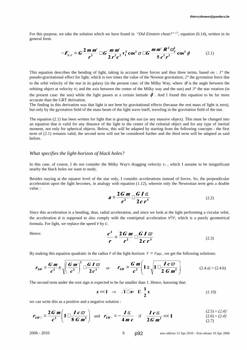
For this purpose, we take the solution which we have found in “Did Einstein cheat?” [7], equation (6.14), written in itsgeneral form.
(2.1)
This equation describes the bending of light, taking in account three forces and thus three terms, based on : 1° thepseudo-gravitational effect for light, which is two times the value of the Newton gravitation; 2° the gyrotation force due
to the orbit velocity of the star in its galaxy (in the present case: of the Milky Way, where α is the angle between theorbiting object at velocity v1 and the axis between the center of the Milky way and the sun) and 3° the star rotation (in
the present case: the sun) while the light passes at a certain latitude ϕ . And I found this equation to be far moreaccurate than the GRT derivation.The finding in this derivation was that light is not bent by gravitational effects (because the rest mass of light is zero),but only by the gyrotation field of the mass beam of the light wave itself, traveling in the gravitation field of the star.
The equation (2.1) has been written for light that is grazing the sun (or any massive object). This must be changed intoan equation that is valid for any distance of the light to the center of the celestial object and for any type of inertialmoment, not only for spherical objects. Below, this will be adapted by starting from the following concepts : the firstterm of (2.1) remains valid, the second term will not be considered further and the third term will be adapted as saidbefore.
What specifies the light-horizon of black holes?
In this case, of course, I do not consider the Milky Way's dragging velocity v1 , which I assume to be insignificantnearby the black holes we want to study.
Besides staying at the equator level of the star only, I consider accelerations instead of forces. So, the perpendicularacceleration upon the light becomes, in analogy with equation (1.12), wherein only the Newtonian term gets a doublevalue :
(2.2)
Since this acceleration is a bending, thus, radial acceleration, and since we look at the light performing a circular orbit,the acceleration a is supposed to also comply with the centripetal acceleration v²/r, which is a purely geometricalformula. For light, we replace the speed v by c.
Hence:(2.3)
By making this equation quadratic in the radius r of the light-horizon r = r MH , we get the following solutions:
or (2.4.a) = (2.4.b)
The second term under the root sign is expected to be far smaller than 1. Hence, knowing that:
(1.19)
we can write this as a positive and a negative solution :
(2.5) ≈ (2.4)+
and if (2.6) ≈ (2.4)- (2.7)
2006 - 2010 6 new edition 13 Apr 2010 – first release 10 Apr 2006
aG mr
G Ic r
= +2
22 3
ω
cr
G mr
G Ic r
2
2 3
2
2= + ω
− = ′ + ′ +′
F Gm mr
Gm mr c
v Gmm R
c rϕ αϕα
ωϕ, cos cos
2
2 52 2 2 12 2
2 2
2 22
rG mc
I cG mLH = ± +
FHG
IKJ2 2
1 12
ω
rG mc
I cG mLH + = +
FHG
IKJ
21
82 2
ωr
Im cLH − = − ω
4I cG m
ω2
12
<<
x x x<< ⇒ + ≈ +1 1 11
2
rG mc
G mc
G IcLH = ± FHG
IKJ +
2 2
2
32
ω
p92
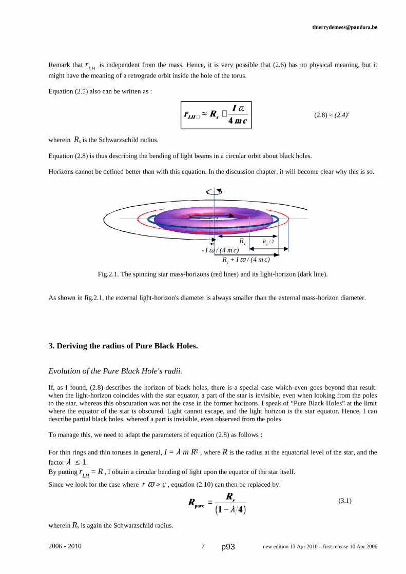
Remark that rLH-
is independent from the mass. Hence, it is very possible that (2.6) has no physical meaning, but it
might have the meaning of a retrograde orbit inside the hole of the torus.
Equation (2.5) also can be written as :
(2.8) ≈ (2.4)+
wherein Rs is the Schwarzschild radius.
Equation (2.8) is thus describing the bending of light beams in a circular orbit about black holes.
Horizons cannot be defined better than with this equation. In the discussion chapter, it will become clear why this is so.
Fig.2.1. The spinning star mass-horizons (red lines) and its light-horizon (dark line).
As shown in fig.2.1, the external light-horizon's diameter is always smaller than the external mass-horizon diameter.
3. Deriving the radius of Pure Black Holes.
Evolution of the Pure Black Hole's radii.
If, as I found, (2.8) describes the horizon of black holes, there is a special case which even goes beyond that result:when the light-horizon coincides with the star equator, a part of the star is invisible, even when looking from the polesto the star, whereas this obscuration was not the case in the former horizons. I speak of “Pure Black Holes” at the limitwhere the equator of the star is obscured. Light cannot escape, and the light horizon is the star equator. Hence, I candescribe partial black holes, whereof a part is invisible, even observed from the poles.
To manage this, we need to adapt the parameters of equation (2.8) as follows :
For thin rings and thin toruses in general, I = λ m R² , where R is the radius at the equatorial level of the star, and the
factor λ § 1. By putting r
LH = R , I obtain a circular bending of light upon the equator of the star itself.
Since we look for the case where r ω º c , equation (2.10) can then be replaced by:
(3.1)
wherein Rs is again the Schwarzschild radius.
2006 - 2010 7 new edition 13 Apr 2010 – first release 10 Apr 2006
r RImcLH s+ ≈ + ω
4
RS
/ 2
RRs
pure =−1 4λb g
Rs + I ω / (4 m c)- I ω / (4 m c)
Rs
p93

We see immediately that, for a ring black hole, when the light horizon reaches the ring's radius itself, this ring's radiusmust have reached about 4/3th of the Schwarzschild radius (the Schwarzschild radius stands for the theoretical sphericalnon-rotating black hole).
Note that the value for the spin rate of that Pure Black Hole equals to ω º c / r , as defined earlier.
Remark that the concept of Pure Black Hole is only theoretical. If the spin velocity becomes close to the speed of light,disintegration of the matter particles is extremely probable.
The graphic evolutes as expected: the higher the spin, the smaller the radius of the light circle becomes. Equation (3.1)is beautifully describing the required radius at the equator level of rotating Pure Black Holes.
Fig.3.1 The Pure Black Hole's light-horizon and mass-horizons
It is then clear that if I depict this graphically, I get fig.3.1. , wherein I show the light-horizon (large dark boundary) andthe mass-horizons (red boundaries) as well.
Spin velocity of Black Holes at the Critical Compression Radius.
In a former paper[8], I have deducted the radius of continuous mass compression at the equator level of spherical stars(with negligible Newtonian-gravitation influence). This deduction was based on the gyrotation field equations for asphere, and we use (1.2) in order to obtain a more general equation. The minus sign signifies “attraction”.
(1.2)
Herein r is the distance to the center of the sphere, R is the radius of the sphere and ω is the spin velocity.
The equatorial compressive gyrotation force is given by the analogue Lorenz force a Rx y= ω Ω (3.2)
and the last term of (1.2) is zero in the direction of the spin axis, so Ω y = 0 .
Hence, the acceleration due to gyrotation at the equator plane is:
(3.3)
At the other hand, we have the following forces: the centrifugal force and the gravitation force. For fast spinning stars,the gravitation force can be neglected, and we find that, in general:
(3.4)
2006 - 2010 8 new edition 13 Apr 2010 – first release 10 Apr 2006
aG mr
RG Ir ctot = + −
FHG
IKJ2
23 2
12
ω
RS
/ 2
< RS
a RG Ir cx = −ω 2
3 22
r rr r r
Ωext ⇐ − −⋅F
HGIKJ
G Ir c
r r
r2
33 2 2
ωωb g
p94

which becomes zero at an equilibrium at the Compression Radius r = R = RC .
The angular velocity at which this occurs is given by :
(3.5)
wherein I have put I = λ m R² as a simplification. The dimensionless parameter λ generally has a value between 0and 1. Remark that R must comply with 4R < Rs .When that angular velocity has been reached, and the black hole became explosion-free, we call the black hole“Perfect”.
Since in this case, the value of the angular velocity is high, the Newtonian gravitation is much smaller than thegyrotational one. By neglecting the Newtonian gravitation, we find that a
tot is zero, for thin ring-shaped pure black
holes, if:(3.6)
Fig.3.2. The Perfect MAG Black Hole with spin velocity ωC , when the Critical Compression has been reached.
The non-explosion condition (3.5), valid for all ring-shaped stars, defines the exterior radius of the ring-shaped spinningstar for a total continuous compression at the equatorial level. By comparing (3.6) with (3.1), there is no way by findinga spinning black hole that is simultaneously Pure and Perfect. Thus, black holes cannot be at the same time pure, andexplosion-free.Indeed, the minimum requirements for the perfect spinning black hole, which cannot explode and which candisintegrate orbiting matter, would then be given by the combination of the metrics, given by fig.3.2. Al these metricscan coexist mathematically.
4. Discussion: Three approaches, three important results.
Orbiting masses at the speed of light.
The first derivation (1.15) for finding horizons resulted in the search of the orbit of matter traveling at the speed of lightabout the spinning star. The meaning of this orbit is however not very clear. Could this be the horizon of the star? Notreally, because this equation goes about matter instead of light. On the other hand, is seems to be correct that no more light can overpass this boundary, as far as matter effectivelydisintegrate at that place.
2006 - 2010 9 new edition 13 Apr 2010 – first release 10 Apr 2006
R RC s= λ 4
RS
/ 2
RS
/ 4
ωC
ω λC
sRG mR R
=−
2
4
p95

(1.21)
But when the matter disintegrates, and when it transform to gamma rays, these rays obey to other rules. The gammarays will be emitted and will –in most of the cases– not be cached by the star. The disintegration of an orbiting objectnear such a star will indeed emit enormous gamma bursts during seconds or minutes. Such gamma bursts are observedand (1.21) is very probably the origin of these observations. Longer bursts are not likely, because partly disintegratedmasses become lighter, and will look up slower orbits, laying at higher distances from the black hole.
Resuming, when one is purely speaking of the concept “event horizon”, which is the circular bending of light, (1.15), or(1.21) , is not exactly the expected solution.
In the first place, the Kerr metric is in contradiction with (1.15) concerning its horizon concept, because of the doubtfulcompliance of horizons with orbiting masses at the speed of light. From (1.15) follows moreover that for non-rotatingstars the limit radius of the mass-horizon becomes:
(4.1) = (1.16)
Surprisingly, the Kerr metric is quasi identical to (1.15) , apart from a constant factor 2 , which allows the Kerr metricto obtain the Schwarzschild radius as a limit for ω = 0 . But this seems more to be an artifice.
The conclusion is that the Kerr metric simply has not to be considered as a matter horizon.
The bending of light and the Kerr metric.
More likely, the bending of light should be the correct approach for defining the concept of “event horizon”. Thishappens in (2.8):
(2.8)
Herein, the Schwarzschild radius is obtained for the limit where ω = 0 . As explained before, it seems much morelogical to consider the circular bending of light as the correct definition of the event horizon.
The concept of the Kerr metric is in disagreement with the solution (2.4) , or (2.8) , but in agreement with (1.15). The
mathematical expression (2.4) has a very simple set-up consisting of a non-rotating term, and a term, linear in ω , whenrotation occurs. Of course, the horizon exists only at the condition that its radius is larger than the star radius.
Comparing both types of horizons
Comparing graphically both equations (1.21) and (2.8) gives the picture (fig. 4.1).
The radius in the upper graphic (circular orbit at the speed of light) raises very quickly with increasing spin velocity.The lower graphic (circular bending of the light), which is barely increasing, starts at the Schwarzschild radius. So, forblack holes with a relatively slow rotation velocity, the “light-horizon” is nearly constant at that same radius. The“mass-horizon” graphic however moves immediately towards higher radii.
2006 - 2010 10 new edition 13 Apr 2010 – first release 10 Apr 2006
ω = ⇒ =02
rR s
r RIm cLH s+ = + ω
4
rR I
mcMHs≈ +2 2
ω
p96
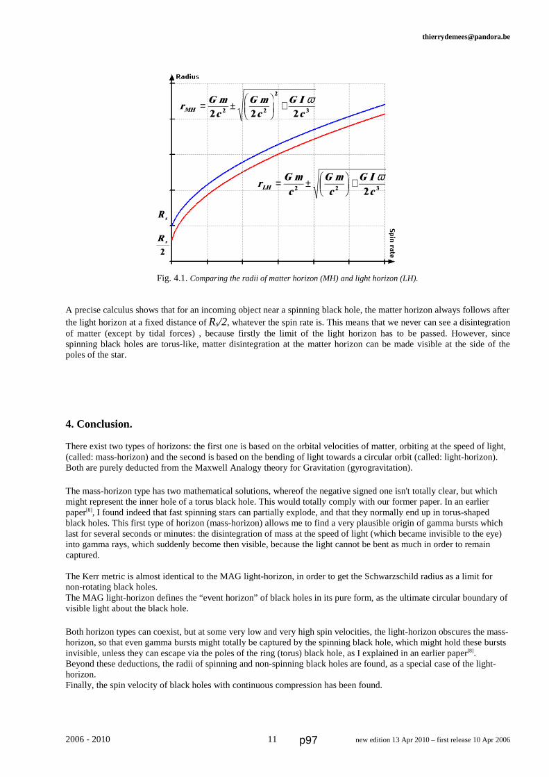
Fig. 4.1. Comparing the radii of matter horizon (MH) and light horizon (LH).
A precise calculus shows that for an incoming object near a spinning black hole, the matter horizon always follows afterthe light horizon at a fixed distance of Rs/2, whatever the spin rate is. This means that we never can see a disintegrationof matter (except by tidal forces) , because firstly the limit of the light horizon has to be passed. However, sincespinning black holes are torus-like, matter disintegration at the matter horizon can be made visible at the side of thepoles of the star.
4. Conclusion.
There exist two types of horizons: the first one is based on the orbital velocities of matter, orbiting at the speed of light,(called: mass-horizon) and the second is based on the bending of light towards a circular orbit (called: light-horizon).Both are purely deducted from the Maxwell Analogy theory for Gravitation (gyrogravitation).
The mass-horizon type has two mathematical solutions, whereof the negative signed one isn't totally clear, but whichmight represent the inner hole of a torus black hole. This would totally comply with our former paper. In an earlierpaper[8], I found indeed that fast spinning stars can partially explode, and that they normally end up in torus-shapedblack holes. This first type of horizon (mass-horizon) allows me to find a very plausible origin of gamma bursts whichlast for several seconds or minutes: the disintegration of mass at the speed of light (which became invisible to the eye)into gamma rays, which suddenly become then visible, because the light cannot be bent as much in order to remaincaptured.
The Kerr metric is almost identical to the MAG light-horizon, in order to get the Schwarzschild radius as a limit fornon-rotating black holes. The MAG light-horizon defines the “event horizon” of black holes in its pure form, as the ultimate circular boundary ofvisible light about the black hole.
Both horizon types can coexist, but at some very low and very high spin velocities, the light-horizon obscures the mass-horizon, so that even gamma bursts might totally be captured by the spinning black hole, which might hold these burstsinvisible, unless they can escape via the poles of the ring (torus) black hole, as I explained in an earlier paper[8].Beyond these deductions, the radii of spinning and non-spinning black holes are found, as a special case of the light-horizon. Finally, the spin velocity of black holes with continuous compression has been found.
2006 - 2010 11 new edition 13 Apr 2010 – first release 10 Apr 2006
R s
2
R s
rG mc
G mc
G IcMH = ±
FHGIKJ +
2 2 22 2
2
3
ω
rG mc
G mc
G IcLH = ± FHG
IKJ +2 2 32
ω
p97

5. References.
1. Feynman, Leighton, Sands, 1963, Feynman Lectures on Physics Vol 2.
2. Heaviside, O., A gravitational and electromagnetic Analogy, Part I, The Electrician, 31, 281-282 (1893)
3. Jefimenko, O., 1991, Causality, Electromagnetic Induction, and Gravitation, (Electret Scientific Cy, 2000).
4. Jefimenko, O., 1997, Electromagnetic Retardation and Theory of Relativity, (Electret Scientific Cy, 2004).
5. De Mees, T., 2003, A coherent double vector field theory for Gravitation.
6. De Mees, T., 2004, Cassini-Huygens Mission.
7. De Mees, T., 2004, Did Einstein cheat ?
8. De Mees, T., 2005, On the shape of rotary stars and black holes.
9. De Mees, T., 2006, On the orbital velocities nearby rotary stars and black holes
10. www.astro.ku.dk, Kerr Metric
2006 - 2010 12 new edition 13 Apr 2010 – first release 10 Apr 2006 p98

Thierry De Mees
How Really Massive are the Super-Massive
Rotating Black Holes in the Milky Way's Bulge?
based on the Maxwell Analogy for Gravitation.
T. De Mees - thierrydemees @ pandora.be
Abstract
The centre of the Milky Way is populated with so-called super-massive black holes. In most of the papers and
books about black holes at the centre of galaxies, the mass is said to be gigantic.
In this paper, we will see how to calculate the mass of these super-massive black holes out of observational data,
by using the Maxwell Analogy for Gravitation, and we see how to make the difference between real physical mass
and apparent (fictive) mass.
We discover that so-called 'super-massive black holes' do not have huge masses at all but that they have an
apparent mass that can be thousands times the real mass. This suggests that the energy of such black-holes could
decrease very fast in relative terms.
Keywords: black hole – horizon – spinning star – super-massive – Maxwell
Method: analytic Notations: metric with comma
1. Basic gyro-gravitation physics for a rotating sphere.
Rotating objects have a velocity-dependent property that is the following. Imagine a sphere that is rotating with an
angular velocity ω . The gravitational field of the sphere is the steady reference field with a velocity that is locally
zero. But the rotation of the particles at a certain velocity, depending from its orbit's radius, will undergo a second
field that is entirely comparable with the magnetic field in electromagnetism. I call this field gyrotation, but
several other names exist in literature, such as co-gravitation field, gravito-magnetic field, etc. This orbital
velocity is locally an absolute velocity. In “A Coherent Dual Vector Field Theory for Gravitation” , I explained
that this second field is generated by the motion of masses.
Fig. 1. If two particles inside a spherical object rotate at their corresponding circular
velocity, they will influence each-other by a gyrotational force.
© Feb. 2008 - March 2009 1
ωωωω
v1
ΩΩΩΩ
m1
g
v2
m2
F2
p99

Thierry De Mees
In fig 1, the mass m1 (a particle of the sphere) orbits at a velocity v1 in the gravitation field g of the sphere. This
motion generates a second field ΩΩΩΩ that is perpendicular on the velocity v1 . This second field will influence any
second mass m2 that travels with a velocity v2 by generating a force F2 that will cause a deviation of the mass m2 .
This force is perpendicular to both the velocity v2 and the gyrotation field ΩΩΩΩ . Mutatis mutandis, the mass m2 will
also deviate any mass m1 in a similar way.
The force F2 can be found by the vector expression :
F2 ⇐ m2 (v2 × ΩΩΩΩ) (1.1)
which can be completed by adding the gravitational force :
F2, tot ⇐ m2 (g + v2 × ΩΩΩΩ) (1.2)
When this scenario is repeated for all the particles of the sphere, the global gravitation is found and the global
second field (the gyrotational field) is found.
For a spinning sphere with rotation velocity ω , the results for the gyrotation at a point p outside the sphere with
mass m is given by the equation (1.3) (5):
(1.3)
wherein • means the scalar product of vectors.
(Reference: adapted from E. Negut). The drawing shows equipotentials of – Ω .
Fig. 1.2
For the level of the equatorial plane, the last term of (1.3) vanishes, and we get a simple expression that is
dependent of the inverse cube of the distance, and, compared with the pure gravitational field, dependent from the
square of the sphere's radius, from the inverse square of the light velocity, and from the sphere's angular velocity.
The result of the expression (1.3) can be put in (1.2) in order to find the total acceleration acting on a arbitrary
mass in motion.
For the equatorial plane, equation (1.2) can generally also be written as :
(1.4)
This equation shows that the second term can have some considerable relative importance, even if the mass is
small. Indeed, the second term can be much larger than 1, depending from the values of the variables. This means
that even if the mass is small, it is still possible to have the impression that we are coping with a massive object.
The equation (1.4) can be expressed more generally, when we consider I the inertial momentum of the central
object:
Since , we get, more generally : (1.5)
In the next chapter, we will analyse these parameters in detail.
© Feb. 2008 - March 2009 2
ωωωω Y p
r
α X
R
Ω ext
GmRr c
r r
r⇐
−−
•FHG
IKJ
2
3 2 25
3ω
ωb g
aG mr
v Rr c
= − +FHG
IKJ2
22
21
5
ω
I m Rsphere =2
52 a
G mr
v Im r c
= − +FHG
IKJ2
221
2
ω
p100
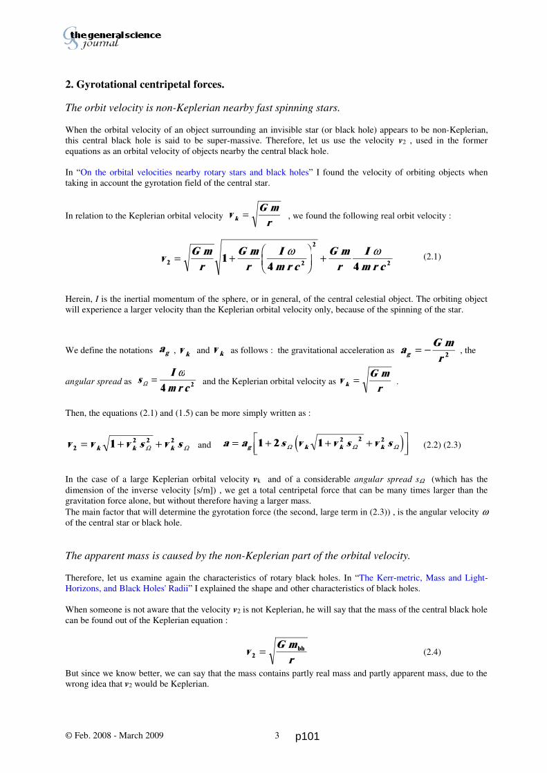
Thierry De Mees
2. Gyrotational centripetal forces.
The orbit velocity is non-Keplerian nearby fast spinning stars.
When the orbital velocity of an object surrounding an invisible star (or black hole) appears to be non-Keplerian,
this central black hole is said to be super-massive. Therefore, let us use the velocity v2 , used in the former
equations as an orbital velocity of objects nearby the central black hole.
In “On the orbital velocities nearby rotary stars and black holes” I found the velocity of orbiting objects when
taking in account the gyrotation field of the central star.
In relation to the Keplerian orbital velocity vG mrk = , we found the following real orbit velocity :
(2.1)
Herein, I is the inertial momentum of the sphere, or in general, of the central celestial object. The orbiting object
will experience a larger velocity than the Keplerian orbital velocity only, because of the spinning of the star.
We define the notations ag , v k and v k as follows : the gravitational acceleration as aG mrg = −
2 , the
angular spread as sIm r cΩ =
ω
4 2 and the Keplerian orbital velocity as vG mrk = .
Then, the equations (2.1) and (1.5) can be more simply written as :
and (2.2) (2.3)
In the case of a large Keplerian orbital velocity vk and of a considerable angular spread sΩ (which has the
dimension of the inverse velocity [s/m]) , we get a total centripetal force that can be many times larger than the
gravitation force alone, but without therefore having a larger mass.
The main factor that will determine the gyrotation force (the second, large term in (2.3)) , is the angular velocity ω
of the central star or black hole.
The apparent mass is caused by the non-Keplerian part of the orbital velocity.
Therefore, let us examine again the characteristics of rotary black holes. In “The Kerr-metric, Mass and Light-
Horizons, and Black Holes' Radii” I explained the shape and other characteristics of black holes.
When someone is not aware that the velocity v2 is not Keplerian, he will say that the mass of the central black hole
can be found out of the Keplerian equation :
(2.4)
But since we know better, we can say that the mass contains partly real mass and partly apparent mass, due to the
wrong idea that v2 would be Keplerian.
© Feb. 2008 - March 2009 3
vG mr
G mr
Im r c
G mr
Im r c2 2
2
21
4 4= +
FHG
IKJ +
ω ω
v v v s v sk k k22 2 21= + +Ω Ω
a a s v v s v sg k k k= + + +LNM
OQP1 2 1 2 2 2
Ω Ω Ωe j
vG m
r2 = bh
p101

Thierry De Mees
So, we get: (2.5)
The total mass (real and apparent) of the rotating star is given by the following expression :
(2.6)
where the first term is the gravitational real mass and the second term the apparent mass.
The equation (2.6) can be written as following, when using (2.2) :
(2.7.a)
Remember that the first part of the equation can be written as (2.7.b)
In the next section, we will analyse the equations (2.7) closer.
Analysis of equations (2.7) and simplification.
Three cases are considered.
Let us consider the case where vk sΩ ≈ 1 . Then the following approximations can be made :
(2.8.a) (2.8.b)
The apparent mass is already considerable here.
When we consider the case where vk sΩ >> 1 , the following approximations can be made, since
1 1 2+ ≈ +x x :
(2.9.a) (2.9.b)
The apparent mass is very important here. This is the case that will be studied further in this paper.
To a certain extend, for vk sΩ >>> 1 , it is even possible to reduce the equations to a more simplified version :
(2.10.a) (2.10.b)
And when vk sΩ << 1 , the following approximations can be made :
© Feb. 2008 - March 2009 4
v v k2 2 1≈ +d i
v v ssk2
221
2≈ +Ω
Ω
vG m m
r2 =+ appd i
m mv rG
+ =app22
m
mv rmG
v v s v s r
mGv s v s
k k k
k kapp
= − =+ +
= + +22
2 2 22
2 22
11
1Ω Ω
Ω Ω
e je j
m
mapp
≈ +1 22d i
m
mv s
v skk
app= +
FHG
IKJ
LNM
OQPΩ
Ω
21
2 2 2
2
m
mv sapp
k≈ 22
Ωb g
m
mvv
app
k
= −22
2 1
≈
vv
v sk
k2 2≈ Ω
p102

Thierry De Mees
(2.11.a) (2.11.b)
Even here, the apparent mass can be of a noticeable importance, if vk sΩ is not too small.
For vk sΩ <<< 1 , we can reduce the equations to a more simplified version :
(2.12.a) (2.12.b)
3. Study of the case vk sΩ >> 1 .
When the case vk sΩ >> 1 is considered, the first thing to do is to verify what the physical balance conditions are
that can comply with the several parameters of the expression vk sΩ . We have to check the physical equilibrium
between the so-called centripetal forces (gravitation and gyrotation) and the centrifugal forces (inertia of mass). In
this paper we will study stars that are stable while spinning.
To obtain the condition vk sΩ >> 1 , it is sufficient to choose the orbit radius r small enough, but still r > R.
The condition of non-explosion of the star.
In “On the geometry of rotary stars and black holes” I found the critical radius at which a fast rotating spheric
object will not fall apart at latitudes smaller than 35°16', even at very fast rotation speeds. The generalization for
some other shapes than the sphere are worked out in “The Kerr-metric, Mass and Light-Horizons, and Black
Holes' Radii”, chapter 3, section “Are Pure Black Holes explosion-free ?”. I found the equilibrium between the
corresponding accelerations, and the corresponding explosion-free Critical Radius RC
:
(3.1)
wherein the symbol Rs is the Schwarzschild radius RG mcs =
22
and the dimensionless factor λ is found out of
I = λ m R² . For a sphere, λ = 2/5 and for a thin ring with radius R we have λ = 1. The radius of the black
hole must be equal or less than RC .
Minimum spinning velocity for the validity of equation (3.1).
Remark that the condition for the non-explosion of fast spinning stars is independent from the spinning speed.
However, the expression (3.1) is not applicable for slowly rotating stars, because during the deduction of the
equation (3.1) in the latter mentioned paper, I have supposed that the gravitational part is negligible versus the
gyrotational part. When the gravitational part is not negligible, the star will even better be kept together, and the
critical radius can be considerably larger without any risk for falling apart.
The condition for which (3.1) is precise enough and applicable in this paper as explained in the Appendix at the
end of this paper, where a general study of the explosion-free equilibrium of stars is given.
Also in the mentioned papers, I find that the final shape of fast spinning stars and black holes must be tiny and
ring-shaped.
© Feb. 2008 - March 2009 5
RR
CS=
λ
4
v v v s v sk k k22 3 21
2≈ + +Ω Ω
m
mv s
v sk
kapp≈ + +FHG
IKJ1
2
2 2 2
ΩΩ
m
mv sapp
k≈ +12
Ωb g vv
v sk
k2 1≈ + Ω
p103

Thierry De Mees
Quotient of apparent mass and real mass.
Let us now compare the apparent mass with the real mass. The equation (2.6) , combined with the definition of
vk sΩ , and in which we replace R by the expression of RC that we found in (3.1) , gives us the quotient of the
apparent mass and the real mass :
(3.2.a)
This equation is only valid for fast rotating stars that do not explode, due to the gyrotation force that keeps the star
together, whatever the rotation speed might be.
One might be very surprised to see such huge powers in this equation. However, this is due because we have
assembled several conditions in the same equation. The first condition is that we have considered that the apparent
mass can only be observed by observing the orbit velocity of an orbiting mass about the star or black hole. Thus,
we consider the apparent mass at the level of that orbiting object. One power of the real mass is accounting for the
orbit velocity of the orbiting object, caused by gyrotation. The second condition is that the chosen type of star is
an explosion-free one. A fourth power of the real mass is accounting for this condition!
The case of vk sΩ >>> 1 allows us to maintain only the first term of the right hand of equation (3.2). The second
term becomes negligible.
The equation (3.2.a) can then be simplified as : (3.2.b)
We see that the speed of light is present to the power minus sixth, which induces that there are needed very high
values for the black hole's mass in order to get significant values for the apparent mass.
Observational limitations due to the Light Horizon.
The radius of the Light Horizon rLH of black holes has been calculated in “The Kerr-metric, Mass and Light-
Horizons, and Black Holes' Radii”, chapter 2, section “What specifies the light-horizon of black holes?” and is
given by :
(3.3)
This value is the minimum distance r from the black hole that has to be used in (3.2), because it is not possible to
observe phenomena that are closer to it, at the level of the equatorial plane, wherefore equation (3.3) is applicable.
The condition for non-explosion (3.1) should still be applicable, although it has not yet combined in the equation
(3.3).
Since I m R= λ 2 , and combined with the equation (3.1) , we get as a limit for the light horizon rLH (by
replacing R by RC ) :
(3.4)
wherein the effective radius of the black hole must be equal or less than RC . In (3.4) , we expressed the light
horizon in different ways.
© Feb. 2008 - March 2009 6
m
mG mr c
r cG m
app≈ +LNM
OQP
λ ω
λ ω
5 2 5 2
3 2 6
3 2 6
5 2 5 2
2
8
32
r RG I
cLH s= +ω 2
42
m
mG m
r capp
≈λ ω5 5 2
3 1264
r RG m R
cR
R Rc
RRc
G mc
G mcLH s
Cs
s Cs
s= + = + = + = +λ ω λ ω λ ω λ ω2 2
4
2 2
2
3 3 2
2 2
3 3 3 2
82 4 64
2
8
p104
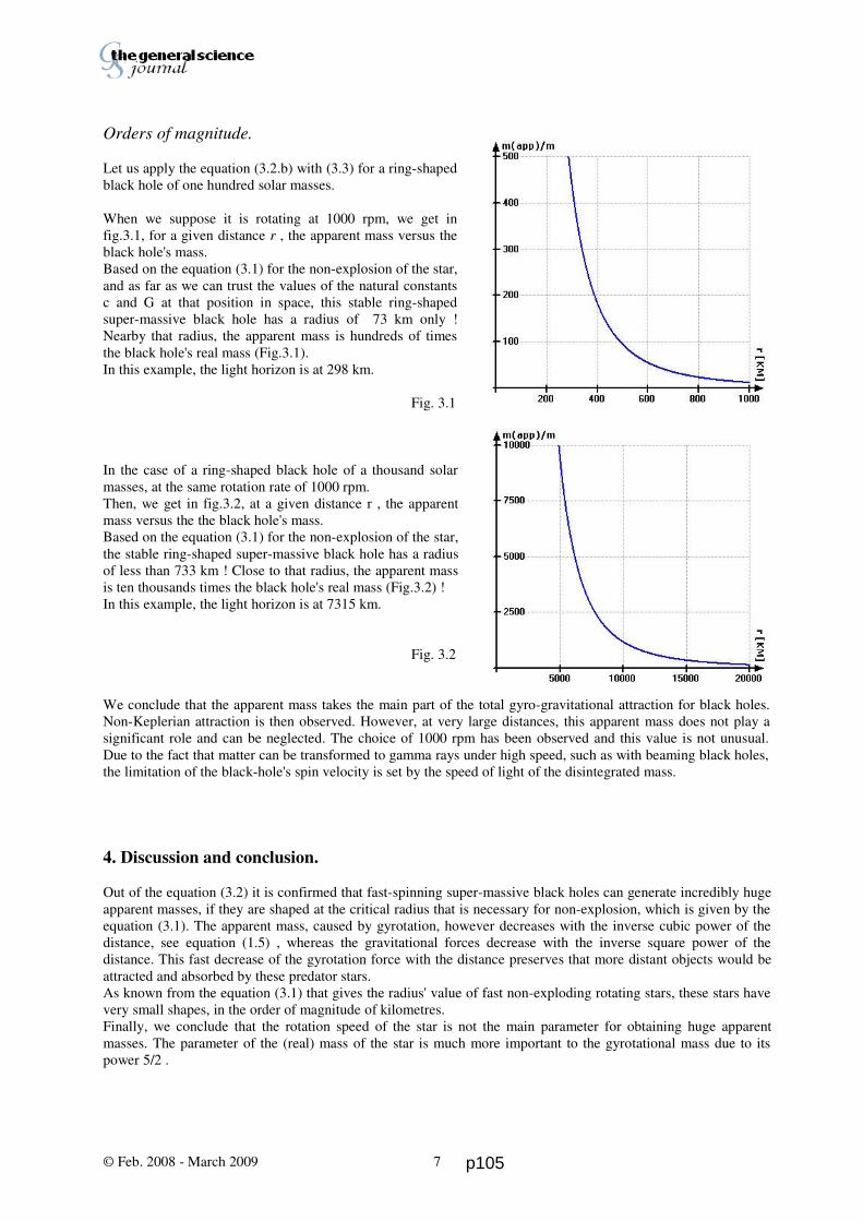
Thierry De Mees
Orders of magnitude.
Let us apply the equation (3.2.b) with (3.3) for a ring-shaped
black hole of one hundred solar masses.
When we suppose it is rotating at 1000 rpm, we get in
fig.3.1, for a given distance r , the apparent mass versus the
black hole's mass.
Based on the equation (3.1) for the non-explosion of the star,
and as far as we can trust the values of the natural constants
c and G at that position in space, this stable ring-shaped
super-massive black hole has a radius of 73 km only !
Nearby that radius, the apparent mass is hundreds of times
the black hole's real mass (Fig.3.1).
In this example, the light horizon is at 298 km.
Fig. 3.1
In the case of a ring-shaped black hole of a thousand solar
masses, at the same rotation rate of 1000 rpm.
Then, we get in fig.3.2, at a given distance r , the apparent
mass versus the the black hole's mass.
Based on the equation (3.1) for the non-explosion of the star,
the stable ring-shaped super-massive black hole has a radius
of less than 733 km ! Close to that radius, the apparent mass
is ten thousands times the black hole's real mass (Fig.3.2) !
In this example, the light horizon is at 7315 km.
Fig. 3.2
We conclude that the apparent mass takes the main part of the total gyro-gravitational attraction for black holes.
Non-Keplerian attraction is then observed. However, at very large distances, this apparent mass does not play a
significant role and can be neglected. The choice of 1000 rpm has been observed and this value is not unusual.
Due to the fact that matter can be transformed to gamma rays under high speed, such as with beaming black holes,
the limitation of the black-hole's spin velocity is set by the speed of light of the disintegrated mass.
4. Discussion and conclusion.
Out of the equation (3.2) it is confirmed that fast-spinning super-massive black holes can generate incredibly huge
apparent masses, if they are shaped at the critical radius that is necessary for non-explosion, which is given by the
equation (3.1). The apparent mass, caused by gyrotation, however decreases with the inverse cubic power of the
distance, see equation (1.5) , whereas the gravitational forces decrease with the inverse square power of the
distance. This fast decrease of the gyrotation force with the distance preserves that more distant objects would be
attracted and absorbed by these predator stars.
As known from the equation (3.1) that gives the radius' value of fast non-exploding rotating stars, these stars have
very small shapes, in the order of magnitude of kilometres.
Finally, we conclude that the rotation speed of the star is not the main parameter for obtaining huge apparent
masses. The parameter of the (real) mass of the star is much more important to the gyrotational mass due to its
power 5/2 .
© Feb. 2008 - March 2009 7 p105

Thierry De Mees
5. References.
1. De Mees, T., General insights for the Maxwell Analogy for Gravitation.
Mercury's perihelion shift and the bending of light grazing the sun.
Solar-, planetary- and ring-system's dynamics.
Fast spinnings stars' and black holes' dynamics.
Spherical and disk galaxy's dynamics.
2. Heaviside, O., A gravitational and electromagnetic Analogy, Part I, The Electrician, 31, 281-282 (1893)
3. Jefimenko, O., 1991, Causality, Electromagnetic Induction, and Gravitation, (Electret Scientific Cy, 2000).
4. Jefimenko, O., 1997, Electromagnetic Retardation and Theory of Relativity, (Electret Scientific Cy, 2004).
Appendix : Critical radius of a spinning star.
The critical radius at which a star will not fall apart even when spinning at a high rate, is deduced from the
equilibrium equation for accelerations, containing gravitation, gyrotation and centripetal accelerations. In this
Appendix, I analyze the outcome of equation (3.1) more generally.
In “On the geometry of rotary stars and black holes”, chapter 3, I wrote the equation (3.3), which can be simplified
for the equator by putting the latitude angle α to zero. The star does not fall apart if this radial acceleration is
negative.
(A.1)
I generalize the case for any angular inertia of the type I = λ m R² and get :
(A.2)
Let us consider four cases.
Case 1 : . (A.3)
Here, the explosion at the equatorial zone can be avoided if . (A.4)
This is the most general situation for fast spinning stars, as we saw in an earlier paper. The gravitational part is
negligible, and we get high spins and small star's shapes.
Case 2 : . (A.5)
Then the total acceleration is always negative and this confirms the case 1.
© Feb. 2008 - March 2009 8
0 12
23 2 2< −
FHG
IKJ −ω R
G IR c
G mR
G m R RG mc
<< −FHG
IKJω
λ2 222
R RG mcC< =
λ
2 2
RG mc
<<λ
2 2
02
2 22
< −FHG
IKJ −ω
λR R
G mc
G m
p106

Thierry De Mees
Case 3 : . (A.6)
Falling apart of the star can be avoided if . (A.7)
This case is applicable to the sun and to the classic stars with a rather slow spin.
Case 4 : . (A.8)
Also here, the total acceleration is then always negative and this confirms again the case 1.
In fine, we can maintain two cases with their corresponding critical radii : cases 1 and 3. The cases 2 and 4 are
only different aspects of the case 1.
© Feb. 2008 - March 2009 9
RG mc
>>λ
2 2
R RG m
C< =ω
23
RG mc
≈λ
2 2
p107

5How Stars in and
outsideGalaxies behave
The most incredible happened. The concept of “Dark Matter” has been grafted on the GeneralRelativity Theory. But was that necessary? Gravitomagnetism proves it wasn't necessary, asclarified in the first paper of this chapter. The constancy of the star's velocity in disc galaxies is justa successful application of Gravitomagnetism.In the second paper, the objects orbiting in flyby with a spinning object are studied more in detail.The results are applicable for satellites that orbit about the Earth, or for the stars outside the disc ofdisc galaxies.
Out of the knowledge of the second paper, the third paper of this chapter evaluates how much timeis needed to form disc galaxies out of spherical galaxies.A dangerous evolution with the Milky Way could happen when mega black holes are formed at itscenter. This is the subject of the fourth and last paper on Galaxies.Savor the most dramatic successes of Gravitomagnetism on the next pages!
p108
Thierry De Mees [email protected]
Deduction of orbital velocities in disk galaxies.or: “Dark Matter”: a myth?
by using Gravitomagnetism.
T. De Mees - [email protected]
Summary
In my paper “A coherent dual vector field theory for gravitation” is explained how simply the Gravitation Theoryof Newton can be extended by transposing the Maxwell Electromagnetism into Gravitation. There exists indeed asecond field, which can be called: co-gravitation-, Gyrotation- (which I prefer), gravito-magnetic field and so on.In this paper, I will call this global theory the Maxwell Analogy for Gravitation (MAG) “Gyro-Gravitation”.
One of the many consequences of this Gyro-Gravitation Theory that I have written down, is that Dark Matter doesnot exist. At least far not in the quantities that someones expect, but rather in marginalized quantities. Manyresearchers suppose that disk galaxies cannot subsist without missing mass that, apparently, is invisible, and whichhas to be taken into account in the classic Newton-Kepler model to better explain the disk galaxies' shapes. An remarkable point is that Gyro-gravitation Theory is not only very close to GRT, but more important, easy tocalculate with, and coherent with Electromagnetism. It is no coincidence that nobody found the same result withGRT, not because GRT would obtain some other result, but because it is almost impossible to calculate with it.A demonstration is again given in this paper, where I deduce the general equations for the orbital velocities ofstars in disk galaxies, based on the assumption of a simple mass distribution of the initial spherical galaxy.
Index
1. Pro Memore : Symbols, basic equations and philosophy. / Maxwell Analogy Equations in short / The definitionof absolute local velocity.
2. Why do some scientists claim the existence of “dark matter”? / The orbital velocity of stars in a disk galaxy /What did Kepler claim ? / Is there a way to get the Kepler law working? / The easy solution: Black Matter /The other reasoning.
3. Pro Memore : Main dynamics of orbital systems. / Why the planets' orbits are plane and prograde / Equationsfor the accelerations nearby spinning stars.
4. From a spheric galaxy to a disk galaxy with constant stars' velocity. / The global stars' velocity in disk galaxies.
5. Origin of the variations in the stars' velocities. / The galaxy's bulge area / The zone near the bulge / The star'svelocities, farther in the disk / The global orbital velocities' equation of disk galaxies.
6. Conclusion : are large amounts of “dark matter” necessary to describe disk galaxies ?
7. References and interesting lecture.
© Feb. 2007 update 16/07/20101 p109
Thierry De Mees [email protected]
1. Pro Memore : Symbols, basic equations and philosophy.
1.1 Maxwell Analogy Equations in short – The two fields.
The formulas (1.1) to (1.5) form a coherent set of equations, similar to the Maxwell equations. The electrical
charge q is substituted by the mass m, the magnetic field B by the Gyrotation ΩΩΩΩ , and the respective constants aswell are substituted (the gravitation acceleration is written as g and the universal gravitation constant as G =(4π ζ)-1. We use sign ⇐ instead of = because the right hand of the equation induces the left hand. This sign ⇐will be used when we want to insist on the induction property in the equation. F is the induced force, v the
velocity of mass m with density ρ. The operator × symbolizes the cross product of vectors. Vectors are written inbold.
F ⇐ m (g + v × Ω Ω Ω Ω ) (1.1)
∇∇∇∇ g ⇐ ρ / ζ (1.2)
(1.3)
where j is the flow of mass through a surface. The term ∂g/∂t is added for the same reasons as Maxwell did: thecompliance of the formula (1.3) with the equation :
It is also expected div ΩΩΩΩ ≡ ∇ ∇ ∇ ∇ ΩΩΩΩ = 0 (1.4)
and ∇∇∇∇× g ⇐ – ∂ ΩΩΩΩ / ∂ t (1.5)
All applications of the electromagnetism can from then on be applied on the gyrogravitation with caution. Also itis possible to speak of gyrogravitation waves.
1.2 The definition of absolute local velocity – The velocities are not relativistic.
When it comes to a competition between GRT and MAG, attention should be paid to two very importantdifferences.
The first one is that the actual MAG that I use is not really relativistic (although one could speak of semi-relativistic; I prefer to speak of Dopplerian). It works like the Newton and the Kepler theories, and like non-relativistic Electromagnetism. Newton and Kepler did not see that the second field existed, caused by the second term in G m m' (1+ v²/c²)/r².This expression is namely the simplest form for the Gyro-gravitation forces, and it is applicable between twoidentical moving masses in one dimension of place (see “A coherent dual vector field theory for gravitation”, lastchapter).This second term, which is very small and which is -by the way- often wrongly seen as an expression related torelativistic phenomena (I would rather say: transversal Doppler-effects), was not observed at that era. The relationto Doppler-effects will not further be discussed in this paper.
The extension of the theory for very fast velocities in non-steady systems has been settled by Oleg Jefimenko inseveral of his books, and is very analogical to what is called “relativistic electromagnetism”, where the fieldretardation -due to the finite velocity of gravitation- has been taken into account.
The consequence of this first difference is that in the framework of MAG, we should only study the kinds ofsteady systems, wherein the retardation of the fields, due to their finite velocity, is not of any crucial importance.
The second difference is that absolute velocity really exists. Not “absolute” with regard of the “centre” of ourUniverse, but “locally absolute” in the observed system wherein the forces interact within a given time-period.This means that the solar system can be studied as a closed system for “short” time periods of several years.However, I found that Mercury's perihelion advance is induced by the sun's motion in the Milky Way (see “Did
© Feb. 2007 update 16/07/20102
div j ⇐ – ∂ρ / ∂ t
c² ∇∇∇∇× ΩΩΩΩ ⇐ j / ζ + ∂g /∂ t
p110
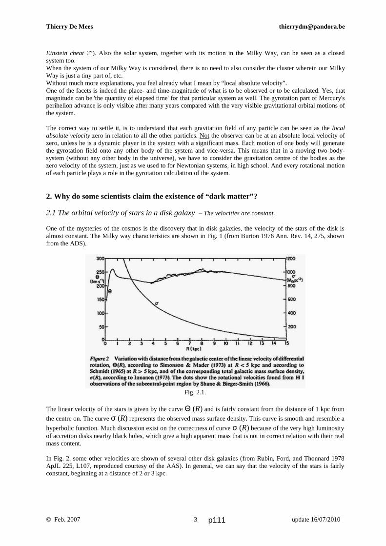
Thierry De Mees [email protected]
Einstein cheat ?”). Also the solar system, together with its motion in the Milky Way, can be seen as a closedsystem too. When the system of our Milky Way is considered, there is no need to also consider the cluster wherein our MilkyWay is just a tiny part of, etc.Without much more explanations, you feel already what I mean by “local absolute velocity”.One of the facets is indeed the place- and time-magnitude of what is to be observed or to be calculated. Yes, thatmagnitude can be 'the quantity of elapsed time' for that particular system as well. The gyrotation part of Mercury'sperihelion advance is only visible after many years compared with the very visible gravitational orbital motions ofthe system.
The correct way to settle it, is to understand that each gravitation field of any particle can be seen as the localabsolute velocity zero in relation to all the other particles. Not the observer can be at an absolute local velocity ofzero, unless he is a dynamic player in the system with a significant mass. Each motion of one body will generatethe gyrotation field onto any other body of the system and vice-versa. This means that in a moving two-body-system (without any other body in the universe), we have to consider the gravitation centre of the bodies as thezero velocity of the system, just as we used to for Newtonian systems, in high school. And every rotational motionof each particle plays a role in the gyrotation calculation of the system.
2. Why do some scientists claim the existence of “dark matter”?
2.1 The orbital velocity of stars in a disk galaxy – The velocities are constant.
One of the mysteries of the cosmos is the discovery that in disk galaxies, the velocity of the stars of the disk isalmost constant. The Milky way characteristics are shown in Fig. 1 (from Burton 1976 Ann. Rev. 14, 275, shownfrom the ADS).
Fig. 2.1.
The linear velocity of the stars is given by the curve Θ (R) and is fairly constant from the distance of 1 kpc from
the centre on. The curve σ (R) represents the observed mass surface density. This curve is smooth and resemble a
hyperbolic function. Much discussion exist on the correctness of curve σ (R) because of the very high luminosityof accretion disks nearby black holes, which give a high apparent mass that is not in correct relation with their realmass content.
In Fig. 2. some other velocities are shown of several other disk galaxies (from Rubin, Ford, and Thonnard 1978ApJL 225, L107, reproduced courtesy of the AAS). In general, we can say that the velocity of the stars is fairlyconstant, beginning at a distance of 2 or 3 kpc.
© Feb. 2007 update 16/07/20103 p111

Thierry De Mees [email protected]
Fig. 2.2.Rotational velocities of stars in several disk galaxies. Most of them have a similar graphic: afast, almost linear increase near the nucleus, a small collaps of the velocity before 5 kpc, and astabilization in the disk at (nearly) one single velocity.
The centre of the bulge has no specific (average) velocity, which result in a zero velocity on the figure. The firstpart of the disk outside the bulge, at nearly 2,5 kpc has often gotten a some higher velocity. And over 4 kpc, thevelocity is almost linear, sometimes sinusoidal. Often, this linearity is almost constant or stays in a short range ofvalues.
2.2 What did Kepler claim ? – The velocities decrease with the distance.
In a planetary system as the solar system, the planets follow a quite simple rule. The square of the orbit velocity ofthe planet is inversely proportional to its distance from the sun. This law has been written down by Kepler.
v ² = G M / r (2.1)
For low velocities, this law is correct and can be applied in this paper as such, even if the correct equation forhigher velocities is somewhat different, as I explained in “On the orbital velocities nearby rotary stars and blackholes” , in chapter 3, equation (3.10).
By increasing distances from the sun, planets will rapidly decrease its orbit velocity. And this law is nothing morethan a geometrical one.There is no a priori reason that the same law wouldn't be true for stars in a galaxy. But reality is different !Equation (2.1) is extremely different from what is observed in galaxies.The purpose of this paper is to find out why this is so.
2.3 Is there a way to get the Kepler law working? – The easy hypothesis: Missing Mass
There is a logical problem, and it should be solved logically. Thus, in order to get disk galaxies complying withKepler's Law, what could be different that we cannot see? Galaxies and stars in general are observed, andclassified by its distance to us, their weight, their motion in relation to us and so on. For long time, we only hadlight as sole measuring instrument to define all these properties. Since a few decades, this has been extended bywaves of other frequencies than just light: X-rays.But still, the method is very uncertain if masses are not bright, but cold.At the other hand, the Kepler Law and Newton's laws only got two variables: mass and distance. The universalgravitation constant could be variable too, but until now, no evidence has been found for this.
© Feb. 2007 update 16/07/20104 p112
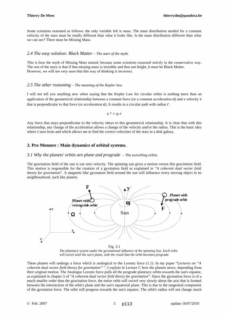
Thierry De Mees [email protected]
Some scientists reasoned as follows: the only variable left is mass. The mass distribution needed for a constantvelocity of the stars must be totally different than what it looks like. Is the mass distribution different than whatwe can see? There must be Missing Mass.
2.4 The easy solution: Black Matter – The start of the myth.
This is how the myth of Missing Mass started, because some scientists reasoned strictly in the conservative way.The rest of the story is that if that missing mass is invisible and thus not bright, it must be Black Matter.However, we will see very soon that this way of thinking is incorrect.
2.5 The other reasoning – The meaning of the Kepler law.
I will not tell you anything new when saying that the Kepler Law for circular orbits is nothing more than anapplication of the geometrical relationship between a constant force (or a constant acceleration a) and a velocity vthat is perpendicular to that force (or acceleration a). It results in a circular path with radius r.
v ² = a r
Any force that stays perpendicular to the velocity obeys to this geometrical relationship. It is clear that with thisrelationship, any change of the acceleration allows a change of the velocity and/or the radius. This is the basic ideawhere I start from and which allows me to find the correct velocities of the stars in a disk galaxy.
3. Pro Memore : Main dynamics of orbital systems.
3.1 Why the planets' orbits are plane and prograde – The swivelling orbits.
The gravitation field of the sun is our zero velocity. The spinning sun gives a motion versus this gravitation field.This motion is responsible for the creation of a gyrotation field as explained in “A coherent dual vector fieldtheory for gravitation”. A magnetic-like gyrotation field around the sun will influence every moving object in itsneighbourhood, such like planets.
Fig. 3.1The planetary system under the gyrotational influence of the spinning Sun. Each orbitwill swivel until the sun's plane, with the result that the orbit becomes prograde.
These planets will undergo a force which is analogical to the Lorentz force (1.1). In my paper “Lectures on “Acoherent dual vector field theory for gravitation” ”, I explain in Lecture C how the planets move, depending fromtheir original motion. The Analogue Lorentz force pulls all the prograde planetary orbits towards the sun's equator,as explained in chapter 5 of “A coherent dual vector field theory for gravitation”. Since the gyrotation force is of amuch smaller order than the gravitation force, the entire orbit will swivel very slowly about the axis that is formedbetween the intersection of the orbit's plane and the sun's equatorial plane. This is due to the tangential componentof the gyrotation force. The orbit will progress towards the sun's equator. The orbit's radius will not change much
© Feb. 2007 update 16/07/20105
SunΩΩΩΩ
ωωωω
X
Y
Z
F
Planet with prograde orbitPlanet with
retrograde orbit
F y
p113

aG m R
r ct = ′ω ω α2
2 252sin
aG m R
r cr = − ′2 2
2 25
ω ω αcos
R
aG m R
r cG m
r
aG m R
r cG m
r
x
y
,
,
sin cos
sin cos sin
tot
tot
= − ′ −
= − ′ −
3
5
3
5
2 2
2 2 2
2 2
2 2 2
ω ω α α
ω ω α α α
Thierry De Mees [email protected]
because the radial component of the gyrotation force is small as well. That component will only slightly changethe apparent mass of the planet, compared with its velocity and its orbit radius. The relationship between theseparameters is given in my paper “On the orbital velocities nearby rotary stars and black holes”, chapter 3,equation (3.10), admitting that the orbit radius remains quasi constant.
When the planet was originally orbiting in retrograde direction, the gyrotation force will push the planet awayfrom the sun's equator. Since the orbit's radius will only change very slightly during this orbital swivelling, theswivelling will continue until the entire orbit becomes prograde, and further converge to the sun's equator.
3.2 Equations for the accelerations nearby spinning stars.
In former papers, we found the equations for the accelerations upon an orbiting object about a spinning star, due tothe gravitation and gyrotation fields. The orbit here is not forming a plane that is going through the star's origin,but an orbit that is parallel to the star's equator. The reason for that choice will follow further on.
(3.1)
(3.2)
These can be written in the more adequate formulation in relation to the radial and the tangential components ofthe gyrotational part :
(3.3)
(3.4)
R is the star's radius, m the star's mass and ω the spinning velocity of the star; α is the angle between the star's
equator and the considered point p , ω' the orbit angular velocity of the point p (the parallel-orbiting object) and rthe distance from point p to the star's centre; c is the light's speed and G the universal gravitation constant.
4. From a spheric galaxy to a disk galaxy with constant stars' velocity.
4.1 The global stars' velocity in disk galaxies.
Relationship between the spherical and the disk galaxy.
We have to consider some other facts before we go for an analysis of the stars' velocities in the disk galaxy: weneed a reconstruction of the original spherical galaxy. And we analyse the disk part of the disk galaxy as well.
fig. 4.1The schematic view of a disk galaxy with radius RRRRe
. The bulge is nearly a sphere or an
ellipsoid. The bulge area, the disk and the fuzzy ends are studied separately. RRRR is the
considered place, r is the variable place (for integration).
© Feb. 2007 update 16/07/20106
- RRRRe
RRRRe
r RRRR
p114

d dV r h r2 2= π d dV r r124= π
ρ ρ1
2
2= h
r
d
d
M r
rMR
1 0
0
b g = =constant
ρπ2
0
02r
Mr R h r
b g b g=
M rMR
r20
0
b g =
v
r
GM r
rg2
2
2= b g
d
d
M r
rMR
2 0
0
b g =
Thierry De Mees [email protected]
In fig. 4.1, we show the schematics of a disk galaxy, with the fuzzy ends of the disk –RRRRe
and RRRRe
, and with the
fuzzy bulge. The considered place p is at a distance RRRR from the galaxy's centre. The variable r is used forintegration purposes.
When we call the spherical galaxy “1” and the disk galaxy “2” the following infinitesimal volumes are :
and
Since for every concentric location r with the respective volumes of cases “1” and “2” we can say thatd dM M1 2= (because only the densities and the volumes got changed) , it follows that ρ ρ1 1 2 2d dV V=
or : (4.1)
The spherical density distribution is given by ρπ1
13
3
4r
M r
rb g b g= by definition,
or : d dM r r r r12
14b g b g= π ρ .
While the expression for the disk galaxy's mass is : d dM r r h r r2 22= π ρ b g b g .
In order to fix the ideas, we go further and we simplify as follows.
Idealizing and simplifying the gravitational part.
The value of M r1b g can be found by assuming that the density distribution of the original spherical galaxy
responds to a simple formula. We could sensibly simplify our analysis by assuming that for every concentric partof the spherical galaxy is valid that :
(4.2)
wherein M0 and R
0 are the total mass and the radius of the bulge. This choice is only made in order to get
simpler results. Besides, such a relationship is not totally unexpected: when we look at a spherical galaxy as asuccession of spherical layers that have the same thickness, from the bulge to the “end” of the galaxy, we canexpect that the masses could possibly be equal for each layer. The volume of each layer increases dramaticallywhile the mass for each layer stays the same. At the “end” of the galaxy, the density decreases dramatically aswell.
Combining (4.1) and (4.2) , we get for the disk galaxy :
(4.3)
Now, we also know that for the disk galaxy: d dM r r h r r2 22= π ρ b g b g , so that when combining with
(4.3) :
or (4.4)
Filling in this equation in the Kepler equation gives :
This means that in this special, simplified case, we get for the overall stars' velocity the simple equation:
© Feb. 2007 update 16/07/20107 p115

vG MRg = 0
0
Thierry De Mees [email protected]
(4.5)
showing that the overall velocity of the stars in the disk of a disk galaxy is constant and equal to the Keplervelocity at the boundary of the bulge. Remark however that we just manipulated formula's mathematically without respecting the full physical meaningduring the deduction. Firstly, in (4.4) we considered only the mass from the galaxy's centre to the place r and notthe mass further away from the galaxy's centre. Secondly, we considered the mass to be concentrated into a pointmass at the galaxy's centre. Although the observed velocities stay in a restricted range, close to the velocity defined in (4.5), the reality showsslightly different local velocities. The origin of these differences interested me, and will be unveiled hereafter.
5. Origin of the variations in the stars' velocities.
5.1 The galaxy's bulge area.
5.1.1 Gyrotation acceleration of stars inside the bulge.
Let us start thinking of a spherical galaxy, whereof the centre is rotating, say, one or more massive black holes.These black holes are fast spinning, and many stars near the center of the spherical galaxy are spinning as well.
When we look at a disk galaxy, we observe that the central bulge is not a sphere like the sun, full of matter, butthat the bulge is a system by itself. The summation of the gyrotation field of all the fast spinning stars of the bulge creates a global, fuzzily spreadgyrotation field, which is difficult to analyze as long as the distribution of the spinning stars is unknown.
Since it is even more difficult to know the local gyrotation acceleration inside the bulge without knowing thelocations of the individual black holes, it seems that the spread of gyrotation would be rather -a priori- random-based. But even if there are several spinning black holes rotating in different directions through the bulge, the globalgyrotation field of the bulge apparently allowed the formation of the disk galaxy. The disk of the galaxy finds itsorigin in a global gyrotation field vector, which is perpendicular to the disk.
5.1.2 The fuzzy gyrotation field of the bulge.
Let us think of the fuzzy gyrotation field of the bulge again.
Theoretically, we get, based on (3.4) and with a good approximation, the tangential gyrotation acceleration :
(5.1)
where ω i symbolizes that the n fast spinning stars can be situated anywhere in the bulge. In fig 5.1 , the meaning
of the symbols is visually shown. The values Di and α
i are variables in time.
The locations and the parameters of the fast spinning stars and black holes are not known. Some statistics could beused here, but this is not the aim of the present paper.
© Feb. 2007 update 16/07/20108
aGc
m RDt
i i i
ii
i
n
= ′=∑
ω ω α5
22
2
21
sin
p116

vG MRg ,0
0
03R Rb g =
aG MRg ,R R R
0
0
03
b g = −
Thierry De Mees [email protected]
fig. 5.1The bulge of the disk galaxy. A mass m at a vertical height H and a horizontal distance R
from the centre is influenced by the gyrotation of black hole i. The surroundings of the bulgeare fuzzy, caused by a random distribution of n black holes which result in unwell definedvectors of the gyrotation fields.
The local thickness of the bulge and its surroundings is symmetric for the z-axis and is determined by (5.1). Thesummation-part in equation (5.1) indeed represents a spread of gyrotation sources that has a standard deviationand results in a Gaussian probability curve around the x-y-plane, but also an axi-symmetric one about the z-axis.Even if the individual black holes are distributed randomly and asymmetrically, we may assume that the x-y- andthe z-distribution are Gaussian. This means that also in the z-direction, a number of stars inside and outside thebulge could have been trapped by some black holes whose rotation axis lays parallel to the x-y-plane.
The radial component of the gyrotation acceleration, as given in (3.3), is valid here as well, but its influence withregard to the stars' velocities is not significant compared to the gravitation part.
Concerning the influence of gyrotation and gravitation for the stars' velocities in the bulge, I expect that theeffective gyrotation acceleration in the bulge is low, because in (5.1), the number of fast spinning black holes willprobably be several thousands of times less than the total number of stars in the bulge. Moreover, the orientationof the fields of each black hole's gyrotation field will be randomized, so that the sum of all such fields will be verylimited. It follows that the gravitational acceleration is dominant inside and nearby the bulge.
5.1.3 Gravitational acceleration in the bulge.
Let us do now the easiest part of the work: the gravitation acceleration of the bulge. When the motion of the starsis not taken into account, we speak of pure gravitation. The Newton's law for the gravitation acceleration inside
homogene full spheres gives, at a radius RRRR :
(5.2)
With the little information we have got about the bulge, this is the best possible equation. The minus sign showsan attraction.
5.1.4 Stars' velocities in the bulge.
If only the gravitational part of the accelerations is significant for the orbital velocities, the star's orbital velocity at
a radius RRRR is defined by :
(for 0 < RRRR < R0) (5.3)
© Feb. 2007 update 16/07/20109
R ms
H X
Z
ωi D
i
mi
αi
p117
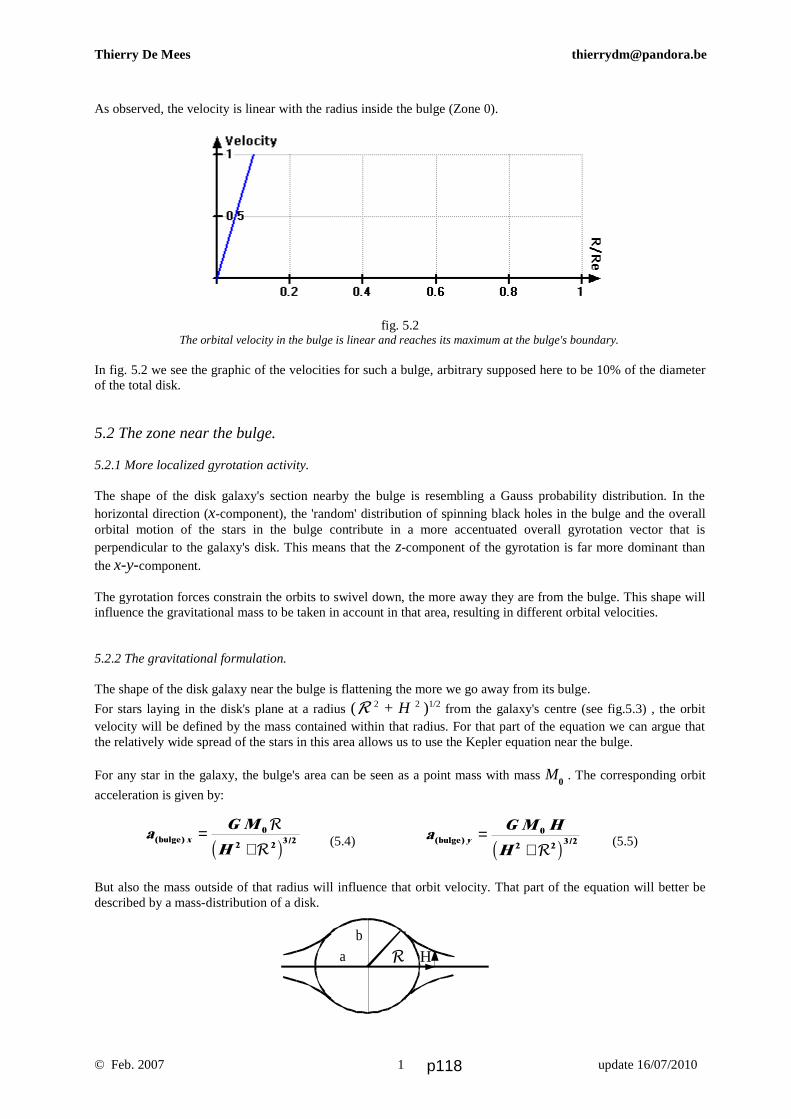
aG M H
Hy( ) /bulge =
+0
2 2 3 2Rc h
Thierry De Mees [email protected]
As observed, the velocity is linear with the radius inside the bulge (Zone 0).
fig. 5.2The orbital velocity in the bulge is linear and reaches its maximum at the bulge's boundary.
In fig. 5.2 we see the graphic of the velocities for such a bulge, arbitrary supposed here to be 10% of the diameterof the total disk.
5.2 The zone near the bulge.
5.2.1 More localized gyrotation activity.
The shape of the disk galaxy's section nearby the bulge is resembling a Gauss probability distribution. In thehorizontal direction (x-component), the 'random' distribution of spinning black holes in the bulge and the overallorbital motion of the stars in the bulge contribute in a more accentuated overall gyrotation vector that isperpendicular to the galaxy's disk. This means that the z-component of the gyrotation is far more dominant thanthe x-y-component.
The gyrotation forces constrain the orbits to swivel down, the more away they are from the bulge. This shape willinfluence the gravitational mass to be taken in account in that area, resulting in different orbital velocities.
5.2.2 The gravitational formulation.
The shape of the disk galaxy near the bulge is flattening the more we go away from its bulge.
For stars laying in the disk's plane at a radius (R 2 + H 2 )1/2 from the galaxy's centre (see fig.5.3) , the orbitvelocity will be defined by the mass contained within that radius. For that part of the equation we can argue thatthe relatively wide spread of the stars in this area allows us to use the Kepler equation near the bulge.
For any star in the galaxy, the bulge's area can be seen as a point mass with mass M0 . The corresponding orbit
acceleration is given by:
(5.4) (5.5)
But also the mass outside of that radius will influence that orbit velocity. That part of the equation will better bedescribed by a mass-distribution of a disk.
© Feb. 2007 update 16/07/20101
ab
R H
aG M
Hx( ) /bulge =
+0
2 2 3 2
R
Rc h
p118

D D* γ β
H
dcos d d
coscos
( , ) * /a
G r h r r H r r
Hr
r DR
R
Rα
ρ α α
αβ
=+ −
+ −FHG
IKJ
b g b g b ge j2 2
2
3 2
Thierry De Mees [email protected]
fig. 5.3The bulge area seen as a ellipsoid. A star, orbiting at a distance (R 2 + H 2)1/2 , will get agravitational influence which is equivalent to a point mass of the size of the bulge's mass.
For simplicity, we consider the bulge as a sphere with a radius R0 .
I will now find the gravity formulation for the disk outside the bulge. Then only, I will be able to deduct a globalformulation for the star's velocities nearby the bulge, and at any place in the disk as well.
5.3 The star's velocities, farther in the disk.
5.3.1 The basic gravitational equations.
Although (5.4) is an approximation for stars that are close to the bulge, it is quite close to reality. This will beclear when we analyse the disk's velocities. Hereafter, I deduct the detailed acceleration equations for any place inand close-by the disk.
fig. 5.4A star with mass m orbits about the bulge's nucleus. The infinitesimal ring of a certaindensity and height will be integrated in order to find the orbital velocity of the star.
In fig. 5.4 , r is the variable radius, R the horizontal distance and H the height of the star with mass m.
Following geometrical equations are valid : L² = H² + l² and D² = R² + H². (5.6.a) (5.6.b)
Remark that, for simplicity, we consider a disk with thickness zero. In reality, the disk's thickness is not zero,especially nearby the bulge. Therefore, the deduction hereafter is only valid at a certain distance of the bulge.
Now d d dM r h r r r= ρ αb g b g and dd
( , ) *
*
a GML
DLr DR α =
2(5.7.a) (5.7.b)
where d ( , ) *a r DR α is the infinitesimal centripetal acceleration in the direction of D * .
Also: lr
=−R cos
cos
αβ
and D r H* cos2 2 2= − +R αb g . (5.8.a) (5.8.b)
Thus, with (5.7.a) , (5.7.a) , (5.8.a) and (5.8.b) , equation (5.7.b) becomes :
(5.9)
.
Now : tansin
cosβ α
α=
−rrR
and cos tan/β β= +
−1 2 1 2c h . (5.10.a) (5.10.b)
© Feb. 2007 update 16/07/20101
d αd r
αrR
h/2ll
m
L
l
p119

dcos d d
cos( , ) /
aG M
Rr r
H r rr xR
R
R Rα π
α α
α=
−
+ + −0
02 2 2 3 22 2
b gc h
dd d
cos( , ) /
aG M
RH r
H r rr zR
R Rα π
αα
=+ + −
0
02 2 2
3 22 2c h
a a rr x
R
r x
e
R
R
R( , ) ( , )d d dα
π
α α= zz0
2
0
a a rr z
R
r z
e
R
R
R( , ) ( , )d d dα
π
α α= zz0
2
0
aG M
RH
H H
R H
H H R Rx
e
e e
R
RR
R R R RR
R
R R R( )
sin cos
sin cos
sin cos
sin cosdα
π
πα α
α αα α
α αα= +
+ + + −− +
+ + + −
L
NMM
O
QPPz0
0
2 2
2 2 2 2 2 2
02 2
2 2 2 2 202
00
2
2 2 2c h c h
Thierry De Mees [email protected]
Using (4.3) , we find : dcos d d
cos( , ) * /
aG M
R
H r r
H r rr DR
R
R Rα π
α α
α=
+ −
+ + −0
0
2 2
2 2 2 3 22 2
b ge jc h
(5.11)
In order to find the horizontal and the vertical component of the acceleration, a projection with angle γ is needed.
Due to symmetry, I disregard the y-component in the plane of the disk.
which result in a multiplication of d ( , ) *a r DR α with cosγ for d ( , )a r xR α and with sinγ for d ( , )a r zR α :
Therefore, notice that : tancos
γα
=−HrR
(5.12)
Using (5.10.b) for the angle γ , and (5.12) , the following components are found:
(5.13)
and
(5.14)
Equation (5.14) is different from zero if H ≠ 0 . From (5.13) and (5.14) follow that the orientation γ of the
infinitesimal vector d a is given by (5.12).
The integration of both (5.13) and (5.14) has to be taken between the following limits (the same limits are validfor the x- and the z-component).
and (5.15) (5.16)
Remember that for the bulge part, we have got another equation. Of course, the integrals (5.15) and (5.16) are
meant to be non-trivial. The integral from 0 to 2π corresponds to twice the integral from 0 to π .
5.3.2 Finding the gravitational equations in the disk.
In the first place, we will integrate the x-component. Remember that the parameters R and H must be taken
constant during the integration. H is not supposed to describe the profile of the galaxy.
Integrating first for r , we find :
(5.17)
This integral has been taken between R0 and R
e .
Also the z-component can easily be integrated for r , which gives the following result:
© Feb. 2007 update 16/07/20101 p120

aG M
R
H
H H
H R
H H R Rz
e
e e
R
R R
R R R RR
R
R R R( )
cos
sin cos
cos
sin cosdα
π
πα
α αα
α αα=
−
+ + + −−
−
+ + + −
L
NMM
O
QPPz0
02 2 2 2 2 2
0
2 2 2 2 202
00
2
2 2 2
b gc h
b gc h
aG M
RR
R Rx H
e
e e
R
R
R R R RR R R R( )
cos cosdα
π
π α αα= =
+ −−
+ −
LNMM
OQPPz0
0
02 2
0
202
00
2
2 2 2
aG MR
RR
R
RHe
e
e
eR
R
R R R
R R
R R R R
R
R,disk = =
−−
−
FHG
IKJ
LNMM
OQPP
−−
−−
FHG
IKJ
LNMM
OQPP
RS|T|
UV|W|
00
02
0
0
0
0
2
2 4
2
4
2ππ π
b g b g b g b gF F, ,
aG M G M
RRR
R
RHe
e
e
eR
R
R
R R R
R R
R R R R
R
R,tot = = +
−−
−
FHG
IKJ
LNMM
OQPP − −
−−
FHG
IKJ
LNMM
OQPP
RS|T|
UV|W|
00
20
02
0
0
0
0
2
2 4
2
4
2ππ π
b g b g b g b gF F, ,
vG M G M
RR
RR
RH
e
e
e
e
RR
R
R R
R R
R R R
R
R, tot = = +
−−
−
FHG
IKJ
LNMM
OQPP
−−
−−
FHG
IKJ
LNMM
OQPP
RS|T|
UV|W|
00 0
02
0
0
0
0
2
2 4
2
4
2ππ π
b g b g b g b gF F, ,
Thierry De Mees [email protected]
(5.18)
This integral has been taken between R0 and R
e as well.
Since the integration of (5.17) and (5.18) to α is complicated, I could integrate it numerically from 0 to 2π .However, I consider that stars at a certain distance H will orbit in a plane under a certain angle with the disk, but Idon't expect a significant difference of velocity compared with stars which lay in the disk's plan.Thus, H = 0 is a valid option in order to get a first idea of the orbital velocities of the stars. This makes (5.17)considerably simpler.
(5.19)
By putting aside the factor G M R0 02πb g , we look at the remaining part between the brackets and integrate it.
Therefore, remark that the integral from 0 to 2π corresponds to twice the integral from 0 to π .
(5.20)
wherein F(x, π/2) is the Complete Elliptic Integral of the First Kind.
The equation (5.20) combined with (5.4) wherein we set H = 0 form the overall equation for the orbitalacceleration of the stars of the disk galaxy, simplified for stars in the disk's plane, and according the massdistribution of equation (4.2).
(5.21)
In the next section, I will deduce the orbital velocities for stars in the disk galaxy and find the correspondinggraph.
5.4 The global orbital velocities' equation of disk galaxies.
The equation for the orbital velocities of the stars in the disk galaxy follows out of v ² = a R .
(5.22)
This equation (5.22) gives the orbital velocity equation in the disk's plane for R0 < R < R
e . Remark that these
velocities are only initial velocities, just after the orbit swivelling.
© Feb. 2007 update 16/07/20101 p121
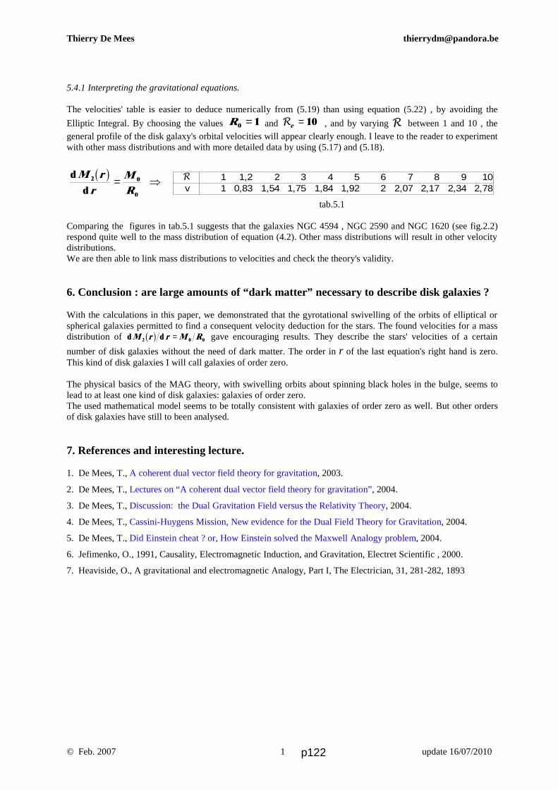
R 1 1,2 2 3 4 5 6 7 8 9 10v 1 0,83 1,54 1,75 1,84 1,92 2 2,07 2,17 2,34 2,78
d
d
M r
rMR
2 0
0
b g =
Thierry De Mees [email protected]
5.4.1 Interpreting the gravitational equations.
The velocities' table is easier to deduce numerically from (5.19) than using equation (5.22) , by avoiding the
Elliptic Integral. By choosing the values R0 1= and Re = 10 , and by varying R between 1 and 10 , thegeneral profile of the disk galaxy's orbital velocities will appear clearly enough. I leave to the reader to experimentwith other mass distributions and with more detailed data by using (5.17) and (5.18).
⇒
tab.5.1
Comparing the figures in tab.5.1 suggests that the galaxies NGC 4594 , NGC 2590 and NGC 1620 (see fig.2.2)respond quite well to the mass distribution of equation (4.2). Other mass distributions will result in other velocitydistributions.We are then able to link mass distributions to velocities and check the theory's validity.
6. Conclusion : are large amounts of “dark matter” necessary to describe disk galaxies ?
With the calculations in this paper, we demonstrated that the gyrotational swivelling of the orbits of elliptical orspherical galaxies permitted to find a consequent velocity deduction for the stars. The found velocities for a massdistribution of d dM r r M R2 0 0b g = gave encouraging results. They describe the stars' velocities of a certain
number of disk galaxies without the need of dark matter. The order in r of the last equation's right hand is zero.This kind of disk galaxies I will call galaxies of order zero.
The physical basics of the MAG theory, with swivelling orbits about spinning black holes in the bulge, seems tolead to at least one kind of disk galaxies: galaxies of order zero. The used mathematical model seems to be totally consistent with galaxies of order zero as well. But other ordersof disk galaxies have still to been analysed.
7. References and interesting lecture.
1. De Mees, T., A coherent dual vector field theory for gravitation, 2003.
2. De Mees, T., Lectures on “A coherent dual vector field theory for gravitation”, 2004.
3. De Mees, T., Discussion: the Dual Gravitation Field versus the Relativity Theory, 2004.
4. De Mees, T., Cassini-Huygens Mission, New evidence for the Dual Field Theory for Gravitation, 2004.
5. De Mees, T., Did Einstein cheat ? or, How Einstein solved the Maxwell Analogy problem, 2004.
6. Jefimenko, O., 1991, Causality, Electromagnetic Induction, and Gravitation, Electret Scientific , 2000.
7. Heaviside, O., A gravitational and electromagnetic Analogy, Part I, The Electrician, 31, 281-282, 1893
© Feb. 2007 update 16/07/20101 p122

aG I
r ct , sin cos sin sin cosΩ = − ′ − −F
HGIKJ
ωω α α α α α2
2 1 33
44
2 2
2c h
Thierry De Mees [email protected]
Swivelling time of spherical galaxiestowards disk galaxies
by using Gravitomagnetism.
T. De Mees - [email protected]
Abstract
This is the second paper dedicated to detailed calculations of disk galaxies. The first is “On orbital velocities in diskgalaxies : “Dark Matter”, a myth?” [2] wherein I explain how to calculate the mass distribution of a disk galaxy andthe orbital velocities of the stars, starting from a mass distribution of the originally spherical galaxy. This is based onthe extended gravitation theory, called “Gyro-Gravitation” or gravitomagnetism. No existence of Dark Matter norany other fancy supposition is needed at all in these calculations.The objective of this paper is to find the mathematical equations related to the time which is needed for the star'sorbit to swivel down to the equator. The total diameter-change of the disk galaxy in the time can be found as well.Yet, these deductions are simplified by keeping constant the bulge's gyrogravitational properties during the process.I leave to the reader to experiment with time-dependent models of gyrogravitational fields in the bulge.An explanation for the very limited windings of our Milky Way's spirals is a direct consequence of this paper.
1. From a spherical to a disk galaxy.
Let us consider a spherical galaxy with a diameter RRRRe .Because the centre contains massive spinning stars orspinning black holes, a gyrotation field will start tomake the stars' orbit swivel, as shown in [2] and [3].After a time t , the radius of the disk galaxy is RRRRe . The
stars beyond RRRRe did only swivel partly, and are not part
of the disk itself.Consider fig.1.1 wherein the spherical galaxy's bulge isshown. The bulge is the group of fast spinning stars thathas a global spin. However, the spin-vectors of theindividual fast spinning stars are oriented variously. Theconsidered star with mass m orbits at a distance r fromthe galaxy's centre.
Fig. 1.1 : Definition of the angle α and θ . The orbital planeis defined by the orbital inclination α in relation to the axis X .
The location of the orbiting star inside the orbit is defined bythe angle θ . The equipotential line of the gyrotation Ω through the orbiting star has been shown as well.
From a former paper[1] we know that the tangentialgyrotational acceleration of a star's orbit is given by:
(1.1)at the place θ = 0.Herein, I is the inertial moment of the bulge, ω itsangular velocity, α the orbit's inclination angle of theconsidered orbiting star, and ω' its orbital angularvelocity, which follows the Kepler law:
(1.2)
wherein M0 is the bulge's mass.
The swivelling equation (1.1) can be represented in agraph, as in fig.1.2.
This means that for prograde orbits, the states of rest aregiven for an orbital inclination of α = 0 and π/4. Forretrograde orbits, they are α = 0 and 3π/4.
© May. 2007 updated 19th July 20101
ωsun
αi
X
Z
Y
Ω
r
ω
α θ
′ = = =ω θb gspherestard
dt
v
r r
G M
r
1 0
p123

R
π r a t tt
tt
200
=FHG
IKJzz ,Ω d d
Thierry De Mees [email protected]
Fig. 1.2. Tangential gyrotational orbit acceleration for θ = 0.
For inclinations between α = 0 and π/4 (prograde), andfor α = 3π/4 and 2π (retrograde), the acceleration tendstowards positive values, resulting in a rotational drifttowards the rotational axis of the Earth. For inclinations between α = π/4 and π/2 (prograde),and for α = π/2 and 3π/4 (retrograde), the accelerationwill much more strongly tend towards negative values,resulting in a rotational drift towards the equatorial axisof the Earth, and retrograde orbits are strongly pushedback into prograde orbits.
We saw in [2] that the -simplified- value of the stars'velocity in disk galaxies has become :
(1.3)
wherein M0 is the mass and R0 the radius of the bulge
(fig.1.3) We have not taken into account thegyrotational forces of the bulge as a part of theattraction force, just for simplicity of the calculations.These forces are to be considered as of secondary order.
This means that (1.2) will become, after the swivelling:
(1.4)
When comparing both equations, the factor r -1/2
becomes R0-1/2 after time.
Fig. 1.3: The schematic view of a disk galaxy with aradius Re
. The bulge is nearly a sphere or an ellipsoid.
The bulge area, the disk and the fuzzy ends are studiedseparately. And r is the considered place.
Below, I now will study the swivelling time for thestars' orbits in a simplified form. Consequently, we willreplace some values by approximations or by theiraverage value.
2. The swivelling time from a sphericalgalaxy to a disk galaxy.
The transformation from a spherical galaxy to a diskgalaxy is quite clear. We have seen that randomlyinclined orbits of planets about the Sun have swivelleduntil they arrived to the Sun's equatorial plane. Alsomost of the stars outside the galaxy's bulge swivel to thebulge's equator plane. Out of fig.1.2. follows that at a certain distance r , thepath length between the random inclination angle α ofan orbit lays between zero and π r. The average pathlength is then π r/2 until the equator. And this is also theaverage path length until the swivelling star passes atthe disk's equator for the first time (remember that themotion is an exponential decreasing oscillation).Remark that the complete swivelling will not occurnearby the bulge, due to the fuzzy and strongly variablegyrotation fields in that region.
Integrating (1.2) twice over time gives the time whichthe average star need to reach the disk region.
Hence, (2.1)
To get rid of α in (1.1), let us replace the geometric
function in α of (1.1) by its average value between α =0 and α = π / 2 .
Thus,
(2.2)
Hence, (2.3)
Herein, (2.4)
is the total angular momentum for the n stars in thebulge and r is as defined in fig.1.3, as a simplification.
And when applying the equation (2.2) into (2.1) , byassuming that the average tangential gyrotationalswivelling acceleration is a constant for each orbit withradius r , it brings me, after integration to:
(2.5)
© May. 2007 updated 19th July 20102
- RRRRe RRRRer
′ = = =ω θb gdiskstard
dt
v
r r
G M
R
1 0
0
sin cos sin sin cosα α α α α2 1 33
442− −F
HGIKJ =c h
av
π α α α α α α ππ
2 2 1 33
44 32
0
2
b g c hsin cos sin sin cos− −FHG
IKJz d =
aG I
r ct,Ωc h
b gav
tot= −′π ω ω
6 2 2
ππ ω ω
r at G I
r ctt2
2 12
2
2 22= = −
′,Ωc h
b gav
tot
I I i ii
n
ω ωb g tot=
=∑
1
vG M
Rstar = 0
0
p124

Thierry De Mees [email protected]
and after rearranging, I get the following result for theswivelling time for a given orbit r :
(2.6)
For the choice of the value of ω' , I suggest to take theaverage of equations (1.2) and (1.4), because veryprobably, the change of angular velocity occurs duringthe swivelling, while the angular momentum of thebulge is transmitted to the disk.
(2.7)
The equation (2.6) can then be rewritten as:
(2.8)
The farther away from the bulge, the longer it takes(nearly quadratically) before the disk takes form. At theextremities RRRRe
of the disk, there is still a fuzzy zone of
stars because only a part of the stars did swivel entirely,namely those who whereof the orbit inclinationoriginally was beyond π/4. Closer to the bulge, the disk is quickly generated. Thegrowth velocity of the galaxy's disk decreases steadilyin time.
3. Discussion.
In the equation (2.8) it is the bulge's angular momentumthat is the most difficult to evaluate. Especially becauseit probably evolved from a low value to a higher valuewith time, and maybe there occurred a contraction ofthe central zone.
The time delay which is observed in spirally woundgalaxies such as the Milky Way does not correspond atall to the total lifetime of the galaxy. The reason is thatthere are several phases of time to consider. The starting point is the spherical galaxy with aspinning center, made of spinning stars and eventuallyblack holes. Then follows the swivelling of the orbits, by which thedisk diameter increases steadily, beginning from thecentre and becoming very thin -in cosmic terms- atsome places, causing a hyper-density of the diskcompared with the original density of the sphericalgalaxy.If the original orbit inclination was situated between 0and π/4, the swivelling was originally pointed towardsπ/4. Later, when the disk formed, even stars at an orbit
inclination till π/4 were attracted by the disk and gotswivelled towards the disk. Only at the extremities ofthe disk, the fuzzy part betrays that the inclination tillπ/4 is more difficult to swivel down.The third phase is the formation of the spirals by thecontraction of some hyper-dense zones, even yet after apartial formation of the disk. When observing the actualspiral-gradient, it appears as if the delay of timebetween the formation of the inner and the outer parts ofthe disk were very short, but in fact this delay is muchlonger because the stars that are farther away from thebulge can only form spirals at the time that the disk hasbecome hyper-dense enough at that place, while theinner disk zone has its spirals yet formed.The observed strange form of the spirals, I would rathersay: many parts of spirals, correlate quite well with thisexplanation.
4. Conclusion.
The time for an average orbit-swivelling is proportionalto an exponent 17/8 of the star's orbit radius. Althoughthe found time-equation is only a limited part of theformation time of our actual Milky Way, it allows usalready to have a clearer view on the formation of diskgalaxies.
5. References and interesting lecture.
1. De Mees, T., Introduction to the Flyby Anomaly: the
Gyrotational Acceleration of Orbiting Satellites,
General Science Journal, 2010.
2. De Mees, T., On orbital velocities in disk galaxies :
“Dark Matter”, a myth?, General Science Journal,
2007.
3. De Mees, T., A coherent dual vector field theory for
gravitation, General Science Journal, 2003.
4. Jefimenko, O., 1991, Causality, Electromagnetic
Induction, and Gravitation, Electret Scientific, 2000.
5. Heaviside, O., A gravitational and electromagnetic
Analogy, Part I, The Electrician, 31, 281-282, 1893.
© May. 2007 updated 19th July 20103
tr c
G Irb g b g=′
6 3 2
ω ωtot
′ =ωb gav
1 0
04r
G M
r R
tr c R
G M Irb g b g
= 61 2 17 801 8
3 401 4 1 2ω
tot
p125

Thierry De Mees
© 2010 March 14th , 2010 1
Gravitomagnetic Evolutionary Classification of Galaxies
explained by the Gravitomagnetic Field Theory
T. De Mees - thierrydemees @ pandora.be
Abstract The Milky Way might be a bar galaxy. In this paper, we show that bar galaxies are spiral galaxies with an orientation change of the bulge's gravitomagnetic field. The tilting of the gravitomagnetic field evolves from the bulge to the galaxy's extremities at wave speed and the physical acceleration of the stars away from the disc follow soon. Finally, this will result in a new, slightly elliptical galaxy that will again turn into a disc galaxy and then a spiral galaxy. If the Milky Way really is a bar galaxy, the solar system will some day get a novel acceleration (an apocalyptic sway) towards a new, widely oscillating position in the galaxy. Finally, we come to a Gravitomagnetic Evolutionary Classification of Galaxies that is different from the usual classifications. Key words : gravitation, gravitomagnetism, Milky Way, bar galaxy, evolutionary classification Method : analytical. 1. The galaxy evolution from a spherical to a spirally disc galaxy. Spherical galaxies mostly doesn't remain spherical for ever. They turn to spherical and even disc galaxies, that on their turn become spiral galaxies (fig. 1.1).
Fig.1.1 : The evolution of a spherical galaxy towards a spiral galaxy. Below, we will explain how this happens, due to a number of spinning stars in the center of the original galaxy.
p126
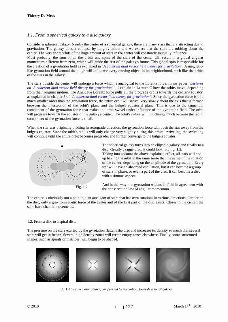
Thierry De Mees
© 2010 March 14th , 2010 2
1.1. From a spherical galaxy to a disc galaxy Consider a spherical galaxy. Nearby the center of a spherical galaxy, there are many stars that are attracting due to gravitation. The galaxy doesn't collapse by its gravitation, and we expect that the stars are orbiting about the center. The very short orbits of the huge amount of stars in the center will constantly mutually influence. Most probably, the sum of all the orbits and spins of the stars of the center will result in a global angular momentum different from zero, which will guide the rest of the galaxy's future. This global spin is responsible for the creation of a gyrotation field as explained in “A coherent dual vector field theory for gravitation”. A magnetic-like gyrotation field around the bulge will influence every moving object in its neighborhood, such like the orbits of the stars in the galaxy. The stars outside the center will undergo a force which is analogical to the Lorentz force. In my paper “Lectures on 'A coherent dual vector field theory for gravitation' ”, I explain in Lecture C how the orbits move, depending from their original motion. The Analogue Lorentz force pulls all the prograde orbits towards the center's equator, as explained in chapter 5 of “A coherent dual vector field theory for gravitation”. Since the gyrotation force is of a much smaller order than the gravitation force, the entire orbit will swivel very slowly about the axis that is formed between the intersection of the orbit's plane and the bulge's equatorial plane. This is due to the tangential component of the gyrotation force that makes the orbit swivel under influence of the gyrotation field. The orbit will progress towards the equator of the galaxy's center. The orbit's radius will not change much because the radial component of the gyrotation force is small. When the star was originally orbiting in retrograde direction, the gyrotation force will push the star away from the bulge's equator. Since the orbit's radius will only change very slightly during this orbital swiveling, the swiveling will continue until the entire orbit becomes prograde, and further converge to the bulge's equator.
The spherical galaxy turns into an ellipsoid galaxy and finally to a disc. Greatly exaggerated, it could look like fig. 1.2. Taking into account the above explained effect, all stars will end up having the orbit in the same sense that the sense of the rotation of the center, depending on the amplitude of the gyrotation. Every star will have an absorbed oscillation, but it can become a group of stars in phase, or even a part of the disc. It can become a disc with a sinuous aspect. And in this way, the gyrotation widens its field in agreement with the conservation law of angular momentum.
The center is obviously not a point but an amalgam of stars that has own rotations in various directions. Farther on the disc, only a gravitomagnetic force of the center and of the first part of the disc exists. Closer to the center, the stars have chaotic movements. 1.2. From a disc to a spiral disc. The pressure on the stars exerted by the gyrotation flattens the disc and increases its density so much that several stars will get in fusion. Several high density zones will create empty zones elsewhere. Finally, some structured shapes, such as spirals or matrices, will begin to be shaped.
Fig. 1.3 : From a disc galaxy, compressed by gyrotation, towards a spiral galaxy.
Fig. 1.2
p127
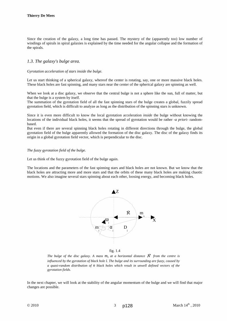
Thierry De Mees
© 2010 March 14th , 2010 3
Since the creation of the galaxy, a long time has passed. The mystery of the (apparently too) low number of windings of spirals in spiral galaxies is explained by the time needed for the angular collapse and the formation of the spirals. 1.3. The galaxy's bulge area. Gyrotation acceleration of stars inside the bulge. Let us start thinking of a spherical galaxy, whereof the center is rotating, say, one or more massive black holes. These black holes are fast spinning, and many stars near the center of the spherical galaxy are spinning as well. When we look at a disc galaxy, we observe that the central bulge is not a sphere like the sun, full of matter, but that the bulge is a system by itself. The summation of the gyrotation field of all the fast spinning stars of the bulge creates a global, fuzzily spread gyrotation field, which is difficult to analyze as long as the distribution of the spinning stars is unknown. Since it is even more difficult to know the local gyrotation acceleration inside the bulge without knowing the locations of the individual black holes, it seems that the spread of gyrotation would be rather -a priori- random-based. But even if there are several spinning black holes rotating in different directions through the bulge, the global gyrotation field of the bulge apparently allowed the formation of the disc galaxy. The disc of the galaxy finds its origin in a global gyrotation field vector, which is perpendicular to the disc. The fuzzy gyrotation field of the bulge. Let us think of the fuzzy gyrotation field of the bulge again. The locations and the parameters of the fast spinning stars and black holes are not known. But we know that the black holes are attracting more and more stars and that the orbits of these many black holes are making chaotic motions. We also imagine several stars spinning about each other, loosing energy, and becoming black holes.
fig. 1.4 The bulge of the disc galaxy. A mass ms at a horizontal distance R from the centre is
influenced by the gyrotation of black hole i. The bulge and its surrounding are fuzzy, caused by a quasi-random distribution of n black holes which result in unwell defined vectors of the gyrotation fields.
In the next chapter, we will look at the stability of the angular momentum of the bulge and we will find that major changes are possible.
R ms
X
Z
ωi
mi
αi D
i
p128

Thierry De Mees
© 2010 March 14th , 2010 4
2. When the global spin of the bulge flips : from a spirally to a turbulent bar galaxy. Before being able to explain the possible reasons of such a tilt change in the bulge, we first lookup the equations that govern the bulge and the disc. 2.1. The acceleration and the swiveling time of the bar galaxy to a newly formed disc galaxy. The value of the acceleration and of the swiveling time of the bar galaxy towards a newly formed disc galaxy is found in “Swivelling Time of Spherical Galaxies Towards disc Galaxies” . In that former paper, I assumed also that the average path length of an arbitrary chosen orbit of the spherical
galaxy was π R / 2 until the equator. The time had then to be found out of a double integration of aΩ to the
time.
In the present case, if the bulge of the bar galaxy tilted with an angle θ , the swiveling path length will now be
reduced to only θ R. The correct time for the swiveling of the bar galaxy into a newly formed disc galaxy will
last (for a place R) :
,
0 0
d d
t t
ta t tθ Ω
=
∫ ∫R
(2.1)
In (2.1) , R is the distance of a certain place on the bar galaxy from the bulge's center, aΩ is the acceleration due
to the gyrotational field of the bulge. After integration (is not time-dependent, only place-dependent in the disc) and rearranging, the result is given by :
2t
a
θΩ
=R
R
(2.2)
Also here, I have neglected the small time retardation due to the wave transmission. A real value for that time can be deduced when we find a way to find the gyrotational acceleration aΩ of the bulge. I will do that in one of the
coming papers. From my former paper, mentioned above, the gyrotational acceleration aΩ is given by (2.3) :
1
2 22
n
i i
s i
IG
ac
ωωπ =
Ω =∑
R (2.3)
wherein we have simplified several parts and where Ii and ωi are the rotation parameters (inertial momentum, the
angular velocity) of the n spinning black holes and stars, which can be moving anywhere in the bulge. The angular
rotation of the star s is ωs . 2.2. Catastrophes in the bulge of galaxies : when a new giant black hole is formed. The sum of all the angular moments L of the k stars and the (n-k) black holes in the bulge is given by :
p129

Thierry De Mees
© 2010 March 14th , 2010 5
(2.4)
wherein I is the inertial momentum and ωωωωi the spin for any of them. We consider here the stars to be spheres and the black holes to be rings, as explained in “On the Geometry of Rotary Stars and Black Holes ”. One would think that equation (2.4) regulates the bulge's gyrotation and the disc's orientation, but that's not true. Indeed, the conservation of angular momentum is important and has to be respected, but the real influence is given by (2.3). In the bulge, an amalgam of stars can clot into a set of mutually orbiting stars. Their global angular momentum will cause a global contraction (collapse) due to the gyrotation field that has a compression that is proportional to the global spin velocity. The quasi-chaotic motion of the black holes and large stars in the bulge can bring them close of stars from the bulge’s edge and attract them. The new upcoming stars and black holes can have totally different spin orientations than the global bulge's angular momentum. But a far more important evolution inside the bulge is that an amalgam of stars can collapse and become a huge black hole with a different spin rate and spin orientation. A single huge black hole can dramatically influence the global gyrotation axis of the bulge. 2.3. Description of the process. The consequence of this process is that the size and the orientation of the total angular momentum of the bulge can evolve dramatically. In cases when a large quantity of stars reduced into a huge black hole, it can get a totally different angular momentum. If the bulge would merge with a group of stars or a galaxy, even small, a strongly different orientation of the bulge's angular momentum is possible. And when such a change happens, the disc zones at the bulge's boundaries will become to get a modified orientation as well: that part will swivel and bit by bit, from the bulge's border to the outer side of the disc, the whole disc will swivel as well. But will this happen unscathed?
Fig.2.1: a bulge tilt occurred by the evolution of the number of newly arisen black holes' tilts, making the disc swivel from the center to the outer parts of the disc
and tare loose the stars by a gyrotation shock wave. We get a bar galaxy. Imagine a bulge that gets tilted compared to the disc. The transmitted gyrotation wave at the speed of light will make swivel the disc by a circular shock wave and the newly tilted part of the disc will gravitationally disturb the rest of the disc. It will attract the boundary and cause fatal issues for planets nearby stars.
L I i i
i
n
==∑ ω
1
p130

Thierry De Mees
© 2010 March 14th , 2010 6
The disc galaxy becomes a bar galaxy with a circular turbulent area at the border of the new forming part and the old disc. 4. Introduction of a new evolutionary classification scheme for galaxies. This leads us to a clear view on the evolutionary classification of galaxies. First we have the spherical galaxy. When the galaxy's center contracts and the orientation of the center becomes well defined, gyrotation flattens the galaxy in to an elliptic galaxy and then a disc galaxy, by making the orbits swivel slowly into prograde orbits. The gyrotation compression augments the disc density and allows stars to get grouped, forming new star activity, and cluttering. This makes it possible to get zones with an increased number of stars and more empty zones. By the constancy of the speed of the stars in the disc galaxy, the arms become spirals.
Fig.4.1: Evolutionary classification of galaxies. From spherical galaxy to an elliptic galaxy, then a disc galaxy and a spiral
galaxy. After a reorientation of the bulge's angular momentum, a bar galaxy with a circularly outside-spreading turbulent zone is created, which a apocalyptic disturbance of the stars and planetary systems of the whole galaxy.
It is possible that, sooner or later, the bulge gets another tilt due to one of the processes I mentioned before. Then the galaxy becomes a bar galaxy, from the bulge towards the rest of the disc. The galaxy swishes into a turbulent object with gravitationally interacting stars by apocalyptic sways. Later on, that slightly elliptical galaxy will again become a disc galaxy. 5. Conclusions. Gravitomagnetism allows a novel evolutionary classification wherein the bar galaxy has a more correct position. The formation of bar galaxies occurs when the bulge's angular momentum changes dramatically, due to the absorption of a small galaxy, a cluster of stars that reduced to a fast spinning huge black hole, or by the natural attraction of stars from the disc with totally different spin orientations. Out-phasing black holes and the ejection of matter from companion stars in dual star systems also change the bulge's angular momentum.
p131
Thierry De Mees
© 2010 March 14th , 2010 7
Most likely, bar galaxies will only form after the stage of disc galaxies and spiral galaxies, and generate a shock wave with a turbulent reorientation of the whole disc galaxy into a newly orientated flat elliptical galaxy and then again to a disc galaxy. 6. References. 1. De Mees, T., 2003, A coherent double vector field theory for Gravitation.
2. De Mees, T., 2004, Lectures on 'A coherent dual vector field theory for gravitation'
3. De Mees, T., 2005, On the Geometry of Rotary Stars and Black Holes.
4. De Mees, T., 2007, Deduction of orbital velocities in disc galaxies, or “Dark Matter” a myth?
5. Feynman, Leighton, Sands, 1963, Feynman Lectures on Physics Vol 2.
6. Heaviside, O., A gravitational and electromagnetic Analogy, Part I, The Electrician, 31, 281-282 (1893)
7. Jefimenko, O., 1991, Causality, Electromagnetic Induction, and Gravitation, (Electret Scientific, 2000).
8. De Mees, T., 2003-2010, list of papers : http://wbabin.net/papers.htm#De%20Mees
p132

6On Dancing and
Beating Asteroids and Satellites
It is if asteroids were alive! The Sun's gyrotation forces make them dance during their orbital motion. In these two papers, Gravitomagnetism proves to comply with all observations on asteroids that were made on hundreds of them during years.
Moreover, Gravitomagnetism discovers that the asteroids that orbit under an inclination angle with the Sun receive veritable beats when they pass the Sun's equator.
Also the fly-by of satellites is studied here because they answer to the same laws of motion.
It is an grateful confirmation of the theory, and it predicts the unobserved!Fly with the asteroids in this chapter!
p133
Thierry De Mees
© Dec. 2007 29/12/2007 - Updates 18/01/2008 and 29/09/2011 1
The Gyro-Gravitational Spin Vector Torque Dynamics of Main Belt Asteroids in relationship with their Tilt and their Orbital Inclination.
described by using
the Maxwell Analogy for gravitation.
T. De Mees - thierrydm @ pandora.be
Abstract Several observational studies of the main belt asteroids showed a direct link between the evolution of the spin vectors and the inclination of their orbit. A study wherein the evolution of 25 main belt asteroids and 125 synthetic objects was computed over 1Myr (E. Skoglöv, A. Erikson, 2002) clearly quantified this link. Verification of these results with the observation of 73 asteroids confirmed the results. Non-gravitational (YORP-/Yarkovsky-) torques are not considered here. Following observational conclusions have been made by E. Skoglöv and A. Erikson: the spin oscillations' amplitude increases with increasing orbital inclination of the asteroid. the largest spin oscillations' amplitudes are found if the initial spin vector lays in the orbital plane. the spin obliquity differences are generally insensitive to the shape, composition and spin rate of the asteroids. there is a significant majority of asteroids with a prograde spin vector compared to retrograde ones. the spin vectors of prograde asteroids are more chaotic than the spin vectors of retrograde asteroids. there are very few asteroids having a spin vector that lays in the vicinity of the orbital plane. the heliocentric distance is relevant for the spin vector behaviour. In this paper it was found that the gyro-gravitation theory, which is the closest Euclid theory to the General Relativity Theory of Einstein, complies very well with these observations. We find that the asteroid's tilt swings continuously during a full orbit. The theoretical values of the cyclic tilt variations are calculated. Keywords: Main Belt Asteroids – gravitation – gyrotation – prograde – retrograde – orbit – precession – nutation. Method: Analytical. 1. Orbital data of the main belt asteroids, by E. Skoglöv and A. Erikson. In our solar system, the orbital evolution of the main belt asteroids is primarily influenced by Saturn and Jupiter. The orbital perturbations are ordinarily periodic in the sense that they vary between certain limits. The spin vectors of asteroids can be influenced by nearby passing planets, by collisions, but there has also been observed a mechanism due to the asteroids' orbital evolution. When I discovered the papers of E. Skoglöv and A. Erikson, I became intrigued by their results. In these papers, the latter mechanism (the one related to the asteroids' orbital evolution) has been observed and reported. This means that the orbital perturbations by Saturn and Jupiter have not been studied here, but only the relationship between both the initial spin orientation and the orbital evolution, in relation with the spin vector evolution of the asteroid. 1.1. Basic data of 25 real objects. Table 1.1 shows which 25 large asteroids have been chosen (E. Skoglöv, A. Erikson, 2002) to perform the observations. The average semi-major axis of the orbit is given and the orbital inclinations: maximal, minimal and average. These orbital variations, caused by Jupiter and Saturn, generate spin vector changes. On these data, the study of E. Skoglöv and A. Erikson has been based on.
p134

Thierry De Mees
© Dec. 2007 29/12/2007 - Updates 18/01/2008 and 29/09/2011 2
Table 1.1 (source : E. Skoglöv, A. Erikson) 1.2. The results of the study for the 25 real objects. In fig.1.2 has been drawn the evolution of the spin vector X = cos , where is the obliquity of the spin vector, which means the tilt of the spin axis from the normal to the orbital plane, as shown in fig.1.1.
The ordinate of Fig. 1.2 shows the minimum and maximum values of this obliquity after a time period of 1 Myr (106 years). The figure also shows the precession frequency ( p = d / d t ) wherein is the precession angle of the spin vector.
(source : E. Skoglöv, A. Erikson)
Fig. 1.2.
Fig. 1.1 : definition of the obliquity of the asteroid's spin vector and the orbital inclination i.
i i
p135

Thierry De Mees
© Dec. 2007 29/12/2007 - Updates 18/01/2008 and 29/09/2011 3
The fig. 1.2 should be read as follows. The spin obliquity of three asteroids, Ceres with iave
= 9.7°, indicated with , Massalia ( iave = 2.0°, ) and Ekard (iave = 18.0°, + ) have been plotted. The initial value X = cos gives the spin obliquity at the time zero, and the maximal and minimal spin obliquities X are given for each of the asteroids, after the time span of 1 Myr. In this discussion we consider our planetary system such that the spin of the sun points upwards. The plotted results give quite a lot of information about the change of the spin vector obliquity over the given time span. The maximal and minimal values are symmetric for Ceres and Massalia. The larger the value of the orbital inclination is, the larger is the X between the maximal and minimal values of the computed spin obliquities X. The X between the maximal and minimal values lays in the region of an initial value X of zero, where the initial spin vector obliquity equals to 90°, and hence is laying in the orbital plane. According to the computation, the initial spin vectors which are perpendicular to the orbital plane of the asteroids, would almost remain unchanged. However, there is a less stable situation when the initial value X is directed upwards than when the vector is directed downwards. The results for the asteroid Ekard are significantly different for both the maximal and the minimal values of the computed spin obliquities X , i.e. a clear tendency towards lower values. This means that the spin vectors tend to point more downwards. 1.3. Basic data of 125 synthetic objects. Besides these 25 real objects, 125 synthetic objects have been created, based on the properties of the 25 real objects but with artificial orbital inclinations iave of 5°, 10°, 15°, 20° and 25°. An artificial precession parameter has been introduced as well, for the use of the numerical extrapolation. I assume that E. Skoglöv and A. Erikson used the best possible numerical integration and the best possible empirical adaptations to obtain the 1 Myr extrapolation for these synthetic objects. Indeed, the exact physical process is up to now unknown, and the results must be interpreted as being entirely empirical. 1.4. The results of the study for the 125 synthetic objects. In fig. 1.3. is computed how the behaviour of the synthetic asteroids changes with time, based on the real data of Ceres. In this case, only the delta is plotted and not the absolute values of computed spin obliquities X. The legend is : orbital inclinations of 5° (), 10° (+), 15° (), 20° () and 25° (*). The same conclusions can be taken as with the real objects.
(source : E. Skoglöv, A. Erikson)
Fig. 1.3
When the inclination of asteroid's orbital plane is very large, there remains a significant X , even for asteroids which are perpendicular to their orbital plane, especially for those perpendicular ones that are pointed downwards.
p136

Thierry De Mees
© Dec. 2007 29/12/2007 - Updates 18/01/2008 and 29/09/2011 4
The instability of the latter asteroids is greater than that of the former ones. Another graphic describes how the maximal values of X can be plotted in relation to the orbital inclinations of the synthetic asteroids. The results are shown in fig. 1.4. Again, we see that the larger the value of the orbital inclination, the larger the maximal X becomes. Both the 25 real objects ( , the least square method gives the lower line) and the 125 synthetic objects ( , the least square method gives the upper line) are shown.
(source : E. Skoglöv, A. Erikson)
Fig. 1.4 The two lines suggest a linear behaviour, but there are clear deviations. The lower end of the individual results of the 125 synthetic objects is showing a steadily slower increase of the maximal X with increasing orbital inclination. Since the number of such asteroids is high, this tendency is representative. 1.5. Observational conclusions. Out of this study, a number of quantitative and qualitative conclusions are made. It follows directly from the fig.1.2 , fig.1.3 and fig.1.4. that the spin oscillations' amplitude increases with an
increasing orbital inclination of the asteroid. Out of fig.1.2 and fig.1.3, the largest spin oscillations' amplitudes are found if the initial spin vector lays in the
orbital plane. It is found from the integration method[9] [10], that the spin obliquity differences are generally insensitive to the
shape, composition and spin rate of the asteroids. It appears[12] that the spin vectors of prograde asteroids are more chaotic than the spin vectors of retrograde
asteroids. Also it has been found[12] that the heliocentric distance is relevant for the spin vector behaviour. 2. The observed spin vector distribution, by A. Erikson. 2.1. The spin vector distribution of 73 asteroids of the Main Belt. Very important data of the asteroids exist because special efforts have been made during the last decade to observe this for long time neglected subject, while much more information was collected about the planets.
p137

Thierry De Mees
© Dec. 2007 29/12/2007 - Updates 18/01/2008 and 29/09/2011 5
(source : A. Erikson, 2000)
Fig. 2.1 In fig. 2.1 there have been several parameters of 73 real asteroids grouped upon one graphic. The total number of the asteroids' spin vectors has been split up in a retrograde and a prograde part, compared with the sun's spin. The left graphic shows the retrograde part and the right part the prograde. The ecliptic latitudes, which are the asteroids' individual spin latitudes above (positive) or below (negative) the individual asteroids' orbital plane, are given by Sin
In fig. 2.2 we find the definition of ecliptic latitude Sin of the asteroid's spin vector : is positive above the orbital plane. The definition of a prograde and a retrograde spin vector is given as well. The spin is prograde if its sense is directed above the orbital plane, and is retrograde if its spin sense is directed below its orbital plane. We have to pay attention with making conclusions from the fig. 2.1, because the orbital inclinations are divided in only two groups, and the spin vector obliquities are not precisely related to these orbital inclinations. Nevertheless, we can find several results. A first discovery is the presence of nearly 64% prograde asteroids versus 36% retrograde asteroids. The second is that in the prograde part, the majority of the asteroids (a quantity of 30) shows an average orbital inclination of less than 10% , against a quantity of 18 with an average orbital inclination of more than 10%. In the retrograde part, we find 11 asteroids with orbital inclination of less than 10%, against 14 asteroids that have an average orbital inclination of more than 10%. Thirdly, there are almost no spin vectors oriented in the vicinity of their own orbital plane (for Sin = 0), especially in the case of orbits with a higher inclination. 2.2. Observational conclusions. Out of this study, a number of qualitative conclusions is made. These conclusion are: Out of fig. 2.1 it appears that there is a significant majority of asteroids with a prograde spin vector compared to
retrograde ones. It has been found [1] [14] that there is an absence of asteroids with their spin vector pointing in the vicinity of their
orbital plane. Also the fig. 2.1 shows this.
Fig. 2.2 : definition of the ecliptic latitude Sin of the asteroid's spin vector : is positive above the orbital plane. Definition of prograde and retrograde spin vector. The spin is prograde if its sense is directed above the orbital plane, and is retrograde if its spin sense is directed below its orbital plane.
i i
p138

Thierry De Mees
© Dec. 2007 29/12/2007 - Updates 18/01/2008 and 29/09/2011 6
3. The Maxwell Analogy for gravitation: equations and symbols. The Maxwell Analogy for gravitation is the closest theory to the General Relativity of Einstein, while the universe remains Euclid and is not curved. The double aspect of the gravitational field is expressed by the Newtonian gravitation field, supplemented with the gravitomagnetic field that I call gyrotation. This latter field has been proposed by Oliver Heaviside at the end of the 19th century. The so-called Gyro-gravitation Theory, which is this very same theory, but including a new physical definition for 'the observer'[2], is suitable to explain celestial mechanics for steady and quasi-steady systems. The retardation of gravitation due to its finite velocity is not taken in account and this does not affect the results noticeably. For the basics of the theory, I refer the reader to my paper: “Analytic Description of Cosmic Phenomena Using the Heaviside Field”[2]. The most relevant parts are summarized in the next paragraphs. 3.1. The general equations of the Maxwell Analogy for gravitation. The gyro-gravitation laws can be expressed in equations (3.1) up to (3.6) below. The electric charge is then substituted by mass, the magnetic field by gyrotation, and the respective constants are also substituted. The gravitation acceleration is written as g , the so-called gyrotation field as , and the universal gravitation constant out of G-1 = 4, where G is the universal gravitation constant. We use the sign instead of = because the right-hand side of the equations causes the left-hand side. This sign will be used when we want insist on the induction property in the equation. F is the resulting force, v the relative velocity of the mass m with density in the gravitational field. And j is the mass flow through a fictitious surface. Bold fonts represent vectors. F m ( g + v ) (3.1)
. g (3.2)
c² j / + g / t (3.3)
div j - / t (3.4)
div . = 0 (3.5)
g - / t (3.6)
It is possible to speak of gyro-gravitation waves with transmission speed c. c2 = 1 / ( (3.7) wherein = 4G/c2. 3.2. Calculation of the gyrotation of a spinning sphere. For a spinning sphere with rotation velocity , the result for gyrotation outside the sphere is given by the vector equation (3.8) . In fig. 3.1, one equipotential line of the gyrotation vector has been traced for a spinning sphere with radius R , a moment of inertia I and a spinning velocity vector at a distance vector r from the sphere's centre. wherein for a sphere : (3.8.a) (3.8.b)
W
r
R
Fig. 3.1 : A spinning sphere with radius R and rotation velocity is generating a rotary gravitation field (or “gyrotation” field) at a distance r from the sphere's centre.
I m R25
2WextG Ir c
r rr
F
HGIKJ2
33 2 2
b g
p139

Thierry De Mees
© Dec. 2007 29/12/2007 - Updates 18/01/2008 and 29/09/2011 7
The value of the gyrotation can be found at each place in the universe, and is decreasing with the third power of the distance r . The factor r represents the scalar vector-product, and this value is zero at the equatorial level. In fig. 3.2 , the definition of the angles and i is shown. The orbital plane of the asteroid is defined by the orbital inclination i in relation to the axis X . The exact location of the asteroid inside the orbit is defined by the angle . The equipotential line of the gyrotation W through the asteroid has been shown as well. Is is clear that the gyrotation of the sun is axis-symmetric about the Z-axis.
Fig. 3.2 : Definition of the angles and i . The orbital plane is defined by the orbital inclination i in relation to the axis X . The location of the asteroid inside the orbit is defined by the angle . The equipotential line of the gyrotation through the asteroid has been shown as well.
Now, we need to write the equation (3.8) in full for each of the components, in the case of the solar sphere. Therefore, we need to know the angle in terms of the inclination i and the position angle , since the scalar vector-product of (3.8 a) is defined by cosr . Therefore we notice that (see fig.3.2): sin cos sinzr r r i (3.8.c) And since sin cos , we get : cos cos sin i (3.8.d) (3.8.e) Hence,
2
3 2 2
3, , 0,0, , , cos sin5x y z z x y z
G m R r r r r ir c r
(3.9)
wherein , , cos cos ,sin ,cos sinx y zr r r r i i (3.10)
The equations (3.9) and (3.10) constitute the detailed vector formula of the equation (3.8). Remark that z = sun . In the next chapters we will analyze the torque which is exerted by the gyrotational part of the gyro-gravitation. Firstly, we have to analyse the effects of gyrotation on the asteroid. Some of the components of the gyrotation will affect the spin or the motion of the asteroid, other components will not affect the asteroid's motion. For the calculation of the torque on the asteroid, we need a few mathematical steps. In the first place, we have to find the relationship between the sun's coordinate system and the most simple possible coordinate system of the asteroid. When we have this mathematical relationship, the torque can be analysed and the conditions for a maximum torque can be found in relation to the orbital inclination of the asteroid and to the obliquity of the spin vector. Let us first express the gyrotation field in the asteroid's local coordinates.
r YX
Z
i
g
a
d
wsun
p140

Thierry De Mees
© Dec. 2007 29/12/2007 - Updates 18/01/2008 and 29/09/2011 8
3.3. Coordinate system transformations. In this chapter, we will study the general implications of the gyrotational field on the asteroid. We define the axial tilt as : = + i (3.11) whereby the angle of axial tilt , the obliquity angle and the angle of orbital inclination i are chosen in the same plane. The axial tilt or spin vector tilt is the tilt of the asteroid compared with the Sun's reference spin vector. The asteroid spins with an angular velocity ast around the Z''-axis. The coordinate system X' Y' Z' is the translated solar coordinate system X Y Z over the distance of the asteroid's orbital radius r and an angle in the orbital plane that is inclined with angle i . We do not consider orbital eccentricity in this paper.
Fig. 3.3. : coordinate system transformation. The asteroid spins with an angular velocity ast . The coordinate system X' Y' Z' is the translated solar coordinate system X Y Z over the asteroid's orbital radius r and an angle in the orbital plane that is inclined with angle i . The spin axis of the asteroid is defined by the angle , which is the axial tilt of the spin vector. The X and Y axes of the solar coordinate system are chosen such that the coordinate system X'' Y'' Z'' is a rotated coordinate system X' Y' Z' over the angle while the axis X' remains identical to X'' . The orbital inclination i is shown here in the same plane as Z Z' .
The spin axis of the asteroid is defined by the angle , which is the axial tilt of the spin vector. The X and Y axes of the solar coordinate system are chosen such that the coordinate system X'' Y'' Z'' is a rotated coordinate system X' Y' Z' over the angle while the axis X' remains identical to X'' . The orbital inclination i is shown here in the same plane as Z Z' and as . We have represented the sun's gyrotation field, which has to be considered uniform in the case of asteroids because of their small sizes. It is clear that the asteroid's axial tilt is not totally defined in space here, because any tilt orientation upon the cone's surface with symmetry axis Z' and angle will comply with the description. However, the role that the exact tilt definition would play is very small, since each place upon the cone will be described once at each orbital revolution. The lack of exact tilt coordinates could play a role for large orbital inclinations, but not for smaller inclinations. Exact tilt coordinates could be preferred for a detailed study of individual asteroids, which is not the aim of this paper. Based on fig. 3.3 in the former chapter, we can write down the related equations between the coordinate system X'' Y'' Z'' and X' Y' Z' . The relationships between both coordinate systems are given by : (3.12.a) and inversely : (3.12.b) The study will be continued in the coordinate system X'' Y'' Z'' . When we want to calculate the torque of the sun's gyrotation onto the asteroid, we will have to rotate the initial gyrotation from the coordinate system X' Y' Z' to the coordinate system X'' Y'' Z'' .
X Y Z X Y Z Y Z" , " , " ' , ' cos ' sin , ' sin ' cosb g b g
X Y Z X Y Z Y Z' , ' , ' " , " cos " sin , " sin " cosb g b g
ast
X'
Z'
Y'
W
0' 0''
Z''
X''Y''
i
90°90°
90°
p141

Thierry De Mees
© Dec. 2007 29/12/2007 - Updates 18/01/2008 and 29/09/2011 9
Hence, (3.13) Now we know the values of the gyrotation on the asteroid in the coordinate system X'' Y'' Z'' and are now ready to calculate the angular acceleration due to this field onto the asteroid. 3.4. The angular acceleration and the torque of the solar gyrotation acting onto an asteroid. In fig. 3.4 we consider an asteroid under the influence of the solar gyrotation W" .
Fig. 3.4 : we consider the asteroid under the influence of the gyrotation W" . The asteroid is rigid, and the only motion-related acceleration is a”z.
Two cases are shown: a velocity that is perpendicular to the X'' axis and one that is perpendicular to the Y'' axis. The gyrotation W" has been split up in its components (W"x, W"y, W"z). When applying the equation (3.1) for each of the components, we get the forces that works onto the asteroid due to gyro-gravitation. Let us firstly write this result as an acceleration only, and omit the gravitational part, because it does not play any role for the torque of the asteroid. Hence, (3.14.a) But the asteroid is rigid, and some accelerations will have no other effect but internal compression of the matter, and the stability of the asteroid. When a”x
or a”y
, or both, are directed towards the asteroid's centre, we get an unstable
asteroid. If both a”x and a”y
are directed outwards, we get a stable asteroid. The study of the asteroid's stability is
made in Appendix A. The motion-related accelerations are : (3.14.b) Only the component which is perpendicular to the asteroid's equator is relevant for the torque. In other words, W”z is not relevant for it. This means that locally, the following gyrotational equations can be written down (see fig. 3.4). and (3.15.a) (3.15.b) However, if we want to describe the totality of the angular acceleration '' on the asteroid, we should re-write (3.1) for angular motions. The purely Newtonian gravitational part is omitted in (3.16) and (3.17). and (3.16) (3.17) For the torque T , we get : and (3.18) (3.19) Remark that T z = 0 . The equations (3.18) and (3.19) can be written in full by using the equation (3.9) , (3.10) and (3.13). So we get:
W W W W W W W Wx y z x y z y z" " ", , , cos sin , sin cosd i d i
a vz y x yb g'' ' ' ' ' W a vz x y xb g
'' '' ' ' W
x y' ' ' ' 1W y x
' ' '' 1 W
Tx yI 1 1 W ' ' Ty xI 1 1 W ''
a a a v v v vx y z y z x z x y y x' ' ' ' " ' ' '' ' ' '' ' ' ' ' ' ' '', , , ,d i d i W W W W
a a a v vx y z x y y x' ' ' ' " '' '' '' '', , , ,d i d i 0 0 W W
p142

Thierry De Mees
© Dec. 2007 29/12/2007 - Updates 18/01/2008 and 29/09/2011 1
221 1
3 2
3 31 sin 2 sin sin 2 sin cos5 4 2x
G m R I ir c
T (3.20)
2
21 13 2
3 cos sin 210y
G m R I ir c
T (3.21)
The equations (3.20) and (3.21) define the solar gyrotational torques on asteroids for each orbital inclination, but also on each location on the orbit. 4. Conditions for a maximal and minimal gyrotation on the asteroid's orbital inclination. 4.1. Forced gyroscopic motion.
Let us consider the forced gyroscopic motion upon the asteroid. The spin axis of the asteroid is the Z''' -axis. We define the following notations for the Euler angles : the precession angle , the nutation angle and the spin angle of the asteroid. In the coordinate system x y z , the angles and are needed to define a location. In the coordinate system x' y' z' , the angles , and are needed to define a location. In the respective coordinate systems, the following relationships are valid. The angular velocity in x' y' z' is given by : (4.1)
(4.2)
(4.3) The angular velocity in x y z is given by : The angular momenta are : (4.4) (4.7) (4.5) (4.8) (4.6) (4.9) wherein we define a cylinder-symmetric asteroid with the inertia momenta : 0 x yI I I and 1 zI I , and wherein
, and are time-derivatives of , and . The equations of motion are then : (4.10) (4.11) (4.12)
x
y
z
sin cos
x
y
z
sin cos
L L L
L L L
L L L
x y z z y x
y z x x z y
z x y y x z
TTT
L I IL I I
L I I
x x x
y y y
z z z
0
0
1
sin cos c h
Fig. 4.1 : Precession and nutation of an asteroid.
p143

Thierry De Mees
© Dec. 2007 29/12/2007 - Updates 18/01/2008 and 29/09/2011 1
wherein L is the angular momentum and T is the solar gyrotation torque that works upon the asteroid.
Notice that in this paper 1 , where 1 is the spinning velocity of the asteroid. Remark that the orientation of the coordinate system X''' Y''' Z''' is not defined yet. We chose it such that the Z'''-axis
corresponds with the Z'' axis, and the X'''-axis corresponds with the torque defined as 2 2xy x y T T T and its
orientation (angle in the coordinate system X''' Y''' Z''' ) given by tan y x T T . The equations of motion become, written in full : (4.13) (4.14) (4.15) Due to the high number of solutions, we should simplify these equations by setting a minimum of restrictions. Suppose that = 0 , or, in other words, the spinning velocity can be seen as a constant. Out of (4.15) and (4.14) we find for the precession velocity : (4.16) The calculation is summarized in Appendix B. Since is not known yet, we can get it from (4.13) by using (4.16). We know that by definition, the nutation and the change of tilt position are equal, thus : = . For the angle we find (see Appendix B) : (4.17) The value of the nutation is however not constant. The angular velocity of the nutation, , can be found by differentiating (4.17) to the time. Knowing that d /d t = d /d , wherein is the orbital velocity of the asteroid, we get (see Appendix B): (4.18) The vector Txy is rotating about the Sun, together with the asteroid's orbit. It fluctuates between a certain minimal value and its maximal value, due to the oscillations of . 4.2. Calculation of the spin vector tilt changes. The calculation of the spin vector tilt changes can be realized by using (4.17), worked out with the equations (C.2) to (C.6) of appendix C. The change of the tilt occurs continuously by the equation (C.6).
I I
I I
I
xy02
0 2 0
0
sin cos sin cos
sin cos cos
cos sin
d i c hd i c hd i
T
cos
I
I I1
02b g
F
HGIKJarctan Txy
I II I2 0
2
02
12
b g
dd
dd
0 00
2
02
12
2 I II I
xyb g T
p144

Thierry De Mees
© Dec. 2007 29/12/2007 - Updates 18/01/2008 and 29/09/2011 1
22 2
03 2 2
0 1
2 9 sin 22 sin5 8 sin
I IG m R ir c I I
(C.6)
After every orbital semicircle, the tilt change with a very tiny portion. It will swing back during the next orbital semicircle. 4.3. Calculation of the precession changes. The precession velocity of equation (4.16) can further be simplified to: (4.19) because of the very small values of . 5. Discussion and conclusions. Based on our theoretical results, we come to a certain number of confirmations of the observed data by E. Skoglöv and A. Erikson. Let us take the points one by one and comment it. The equations (3.20) and (3.21), (C.6), and fig.A.1 are the main theoretical data whereon the correlation can be tested. the heliocentric distance is relevant for the spin vector behaviour. This property follows directly from (3.20) and (3.21). The dependency from the distance to the sun is inverse, with an exponent 3. the spin tilt oscillations' amplitude increases with the increasing orbital inclination of the asteroid. The main theoretical data, see equation (C.6), confirm the increasing values of the oscillations with increasing orbital inclination i and, consequently, of its torque and its precession. the largest spin oscillations' amplitudes are found if the initial spin vector lays in the orbital plane. At an axial tilt of = /2 , the acceleration's values are the largest, according to the main theoretical data. Since the values and are relatively similar for values around = / 2 and for not too important orbital inclinations, there is a good correlation between the observed and the theoretical data. the spin obliquity differences are generally insensitive to the shape, composition and spin rate of the asteroids. This is not what we found theoretically. It is not clear why the observational data do not discover this, but probably the reason is that the high impact of the orbital inclination totally masks the observational data of the other influencing parameters. We found a flaw in the representativity of the graphical concepts of E. Skoglöv and A. Erikson, especially for the fig.1.2 and fig. 1.3. To show this, let us define = arctan(X0) - i , so that = + i = arctan(X0) , and the function X = cos (arctan(X0) – i ) , which is only a transcription of the definition X = cos , apart from the term -i . This function only depends from the orbital inclination i and from the initial, fixed cos . Now we found that the shape of curve that this function represents, is virtually the same as the one of fig.1.2. In other words, the only fact of the inclusion of the orbital inclination i already gives the curve shapes of fig.1.2, totally independently from any observations. The supposed (strong) dependence of the orbit inclination to the spin vector tilt is namely only fictive in that graphic. The same is valid for the function represented by function X = cos (arctan(X0) – i ) - X0 compared with fig.1.3, which supposes a strong dependency from the spin vector obliquity that however is almost only caused by the part of the orbital inclination i. The influence of other parameters appear to be severely masked as well in these graphics. In other words, the choice of associating the tilt with the obliquity angle is unfortunate for observational data, because the real tilt is totally masked by the influence of the inclination i. It would be likely to get the observational data in the form = f ( , i ) .
II I
1
02
p145

Thierry De Mees
© Dec. 2007 29/12/2007 - Updates 18/01/2008 and 29/09/2011 1
the spin vectors of prograde asteroids are more chaotic than the spin vectors of retrograde asteroids. From fig.A.1 it is clear that the stability of the asteroids theoretically comply with these findings. For prograde orbits and for large orbital inclinations, the graph shows a very strong tilt instability, while for retrograde orbits, the graph has a milder instability. However, for prograde orbits and for small orbital inclinations, the tilt instability is very low. Remark that the use of the terms 'prograde' and 'retrograde' in the theoretical part is to be related to the solar spin as a reference, while in the papers of E. Skoglöv and A. Erikson, this means : related to the reference of the ecliptic latitude. For small inclinations, the observational difference is barely noticeable. there is a significant majority of asteroids with a prograde spin tilt vector (0 < < /2) compared to retrograde
ones ( /2 < < ). This property can explained by the theory, since fig.A.1 is asymmetric to the prograde and the retrograde orbits. Indeed, the prograde tilts are fully stable for small prograde orbit inclinations. Since there are more prograde orbiting asteroids, the number of prograde tilts must be higher as well. there is an absence of asteroids with their spin vector pointing in the vicinity of their orbital plane. This follows from the equation (C.6) where the largest deviation of the tilt is obtained if = /2. It also follows from fig.A.1, where most of the orbit is unstable if = /2. 6. References and bibliography. 1. Barucci, M. A., D. Bockelee-Morvan, A. Brahic, S. Clairemidi, J. Lecacheux, and F. Roques 1986. Asteroid spin
axes: Two additional pole determinations and theoretical implications. Astron. Astrophys. 163,261–268.
2. De Mees, T., 2005, Analytic Description of Cosmic Phenomena Using the Heaviside Field, Physics Essays, Vol. 18,
Nr 3.
3. Einstein, A., 1916, Über die spezielle und die allgemeine Relativitätstheorie.
4. Erikson, A. 1999, The spin vector distribution of main belt asteroids. Bull. Am. Astron. Soc. 31,1112.
5. Erikson, A. 2000. The present distribution of asteroid spin vectors and its relevance to the origin and evolution of
main belt asteroids. DLR-Forschungsbericht 2000—37. DLR,Köln.
6. Feynman, Leighton, Sands, 1963, Feynman Lectures on Physics Vol 2.
7. Heaviside, O., A gravitational and electromagnetic Analogy, Part I, The Electrician, 31, 281-282 (1893)
8. Jefimenko, O., 1991, Causality, Electromagnetic Induction, and Gravitation, Electret Scientific, 2000.
9. Laskar, J., and P. Robutel, 1993, The chaotic obliquity of the planets, Nature 361, 608–612.
10. Skoglöv, E. 1999, Spin vector evolution for inner solar system asteroids. Planet. Space Sci. 47,11–22.
11. Skoglöv, E., P.Magnusson, and M. Dahlgren, 1996. Evolution of the obliquities for ten asteroids. Planet. Space Sci.
44,1177–1183.
12. Skoglöv, E., 2001, The Influence of the Orbital Evolution of Main Belt Asteroids, Icarus 160.
13. D. Vokrouhlický, D. Nesvorný, 2006, W.F. Bottke, Secular spin dynamics of inner main-belt asteroids, Icarus 184.
14. Zappalà, V., and Z. Knevžević 1984. Rotation axes of asteroids: Results for 14 objects, Icarus 59,435–455.
p146

Thierry De Mees
© Dec. 2007 29/12/2007 - Updates 18/01/2008 and 29/09/2011 1
Appendix A : Tilt stability study of the asteroids.
From (3.15) it follows that the larger a''z is, the more instable the asteroid's tilt. With (3.20) we see that the most
instable situation occurs if, roughly speaking, = / 2 . But a''z
is not the only factor for stability.
A stable asteroid's tilt is also given by the condition a''x > 0 or a''y > 0 . A labile asteroid is obtained if a''x
< 0 or
a''y < 0 . We have indifference if a''x = 0 or a''y
= 0 . With (3.14.a) and with the angular notation such as in (3.16) and
(3.17), we conclude that tilt stability indifference occurs if W''z = 0. When using (3.9), (3.10) and (3.13), we come to the following conditions for an indifference of the tilt stability :
2 23 cos sin 1tan
3 sin cos sini
i
(A.1)
Graphically, the equation (A.1) has been plotted in fig. A.1.
Fig. A.1.a and b.: Plot of the neutral tilt angle neutral in relation to the angular location and the orbital inclination i. Values of that are higher than neutral (northern semicircle) or lower (southern semicircle) will give a stable asteroid's tilt. Values of that are lower than neutral (northern semicircle) or higher (southern semicircle) will give a unstable asteroid's tilt. Prograde orbits with small inclinations provide very stable tilts, but above an orbit inclination of about /8, the tilts suddenly become very unstable until about 7/8, after which they become stable again for about 0 < < /8 and 7/8 < < Note that the orientation of the tilt in space has only been defined regarding the z-axis, not the x and y axes. The results for the x and y axes are averaged. However, during one orbital rotation, all the possible orientations to the x and y axes are reached. Tilt stability is obtained if W"z
> 0 or 2 2tan 3 cos sin 1 3 sin cos sini i and this occurs if
neutral (northern semicircle) or neutral (southern semicircle); unstable tilt is obtained if W"z < 0 or
2 2tan 3 cos sin 1 3 sin cos sini i and this occurs if neutral (southern semicircle) or
Fig.A.1.a Fig.A.1.b
p147
Thierry De Mees
© Dec. 2007 29/12/2007 - Updates 18/01/2008 and 29/09/2011 1
neutral (northern semicircle). For fig. A.1, this means that the zone between both neutral curves is unstable, but that the zone outside is stable. Roughly speaking, we conclude out of fig. A.1 , that when the orbit inclination is smaller than nearly /8, as well prograde as retrograde, the tilt is highly stable. However, once the orbit inclination is higher than /8, there is a sudden switch to an unstable tilt. Then, the tilt will swing northwards or southwards, depending from the position at that time in the northern or the southern orbit semicircle. Remark that the zone of tilt stability is much wider in for prograde orbits if 0 < i < /8 then for retrograde orbits when 7/8 < i < This the main reason why the planet's tilt in our solar system are stable. Venus' tilt, which is opposite, might have been originated because of an original orbit inclination wherefore i > /8, causing a tilt instability and even a tilt switch, without any collision with other bodies. As known by former papers, the inclined orbits tend to swivel into prograde orbits that are nearly in the Sun's equatorial plane. Note that the orientation of the tilt in space has only been defined regarding the z-axis, not against the x and y axes. The results for the x and y axes are averaged. However, during one orbital rotation, all the possible orientations to the x and y axes are reached. Appendix B : Calculation of the precession and the nutation. Since 0 , from (4.15) we get : tan . Using this in (4.14) gives : (B.1) Wherein tan2 << 2. We can use (B.1) in (4.13) and we obtain : (B.2) or for the nutation angle : (B.3) The nutation velocity is found as follows: since d /d t = d /d , wherein is the orbital velocity of the asteroid, we find : (B.4) which can be simplified to : (B.5) We know that Txy is very small in this application, and hence : (B.6)
tan cos
II I0
22c he j
tan 22
0
022
I II I xy
b g T
F
HGIKJarctan Txy
I II I2 0
2
02 2
b g
dd
dd
F
HGIKJ
FHGG
IKJJ
0 00
2
02
02
12
2
02
12
2
12
I I
I II I
I Ixy
xyb gb gT
T
dd
dd
0 0
02
12
02
02 4
14 2
04
2
2
I I I I
I I I Ixy
xyb gb ge jT
T
dd
dd
0 00
2
02
12
2I II I
xyb g T
p148
Thierry De Mees
© Dec. 2007 29/12/2007 - Updates 18/01/2008 and 29/09/2011 1
The same result as (B.6) can be found by using (B.1) in (4.13) while supposing small enough to be neglected and small enough to consider that tan = . This confirms a good credibility of the parametric choices. Let us work out (B.6). We defined (B.7) Working out (B.6) will need us to find the result of . (B.8) The derivatives are :
2
1 13 2
d 3 cos 2 sin 2 sin sin cosd 5
x G m R I ir c
T
(B.9)
and
2
1 13 2
d 3 sin 2 sin 2d 10
y G m R I ir c
T
(B.10)
We do not write (B.6) in full with the results that we find in (B.9) and (B.10), but it is clear that there is a solution. Appendix C : Detailed estimation of the relevant torques and tilt variations. Since (B.7) is relevant for any value of , we can choose to limit our analysis to the average values of each performed orbital revolution. We get for the values = 0 or = , and = /2 or = - /2 the following results :
2
2 2 1 13 2
2sin
5x yG m R I
r c
T T (C.1)
2 2
2 2 1 13 2 2
0
9 sin 21 sin5 4 sinx y
G m R I ir c
T T (C.2)
And this gives as an average for the total circle:
av
2 22 2 1 1
3 2 2
9 sin 21 1 sin5 4 sinx y
G m R I ir c
T T (C.3)
which can be simplified, when using 1 1 2x x into :
av
2 22 2 1 1
3 2 2
9 sin 22 sin5 8 sinx y
G m R I ir c
T T (C.4)
Equation (4.17) can then be written as follows :
22 20
3 2 20 1
2 9 sin 2arctan 2 sin5 8 sin
I IG m R ir c I I
(C.5)
Since the absolute value of is very small, we can omit the trigonometric function and set approximatively :
dd
dd
ddT T T TT
T Txy
xx
yy
x y
2 2
T T Txy x y 2 2
p149

Thierry De Mees
© Dec. 2007 29/12/2007 - Updates 18/01/2008 and 29/09/2011 1
22 2
03 2 2
0 1
2 9 sin 22 sin5 8 sin
I IG m R ir c I I
(C.6)
Hence, (C.6) is the nutation value after half an orbital revolution, and it will swing back during the second half an orbital revolution. For important inclinations, and especially if they are close to /2, the tilt variations can become up to 3,25 times that of the same asteroid if it would orbit in the sun's equator plane. The same effect occurs with satellites that orbit about the Earth (fly-by anomaly).
p150

Thierry De Mees
© Dec. 2007 29/12/2007 - Updates 18/01/2008 and 29/09/2011 1
Cyclic Tilt Spin Vector Variations of Main Belt
Asteroids due to the Solar Gyro-Gravitation.
described by using the Maxwell Analogy for gravitation.
T. De Mees - thierrydm @ pandora.be
Abstract In the paper “The Gyro-Gravitational Spin Vector Torque Dynamics of Main Belt Asteroids in relationship with their Tilt and their Orbital Inclination” I found the excellent compliance between the observations and the extrapolations of E. Skoglöv and A. Erikson, 2002, and the theoretical deductions according the Maxwell Analogy for Gravitation. This implies namely the existence of the second gravitational field : Gyrotation (Co-gravitation). Six of the seven observations are directly explained by the theory. The seventh observation : “there is a significant majority of asteroids with a prograde spin vector compared to retrograde ones” is explainable by supposing that the asteroids are created, like most of the planets are, prograde. The theory found that the asteroids' spins are expected to end-up as retrograde. Two factors play a role : the speed of change of tilt due to gyrotation, and the other influences like the perturbations by Jupiter and Saturn or the gravitational librations. Here, mainly the gyrotation part is studied analytically and graphically, and commented. Keywords: Main Belt Asteroids – gravitation – gyrotation – prograde – retrograde – orbit – precession – nutation. Method: Analytical. 1. Introduction. This paper is an extension of “The Gyro-Gravitational Spin Vector Torque Dynamics of Main Belt Asteroids in relationship with their Tilt and their Orbital Inclination” wherein the following observations could be confirmed theoretically. the spin oscillations' amplitude increases with increasing orbital inclination of the asteroid. the largest spin oscillations' amplitudes are found if the initial spin vector lays in the orbital plane. the spin obliquity differences are generally insensitive to the shape, composition and spin rate of the asteroids. the spin vectors of prograde asteroids are more chaotic than the spin vectors of retrograde asteroids. there are very few asteroids having a spin vector that lays in the vicinity of the orbital plane. the heliocentric distance is relevant for the spin vector behaviour. there is a significant majority of asteroids with a prograde spin vector compared to retrograde ones. The last observation however is only valid, according the theory, if at the origin, the asteroids were created with a prograde spin, like the majority of the planets. In “Are Venus’ and Uranus’ tilt of natural origin? ” and in “The Titius-Bode law shows a modified proto- gas-planets' sequence.” are explained how the planets are probably created from a solar eruption. If the asteroids' spins are really created prograde, and if a number of asteroids might have changed polarity of spin by collisions, there might also be some of them that just obey the theory, wherein is found that the tilt changes from prograde to retrograde continuously du to the gyrotation force that works on it. In this paper, we look for the interpretation of the quantitative results of the former paper: “The Gyro-Gravitational Spin Vector Torque Dynamics of Main Belt Asteroids in relationship with their Tilt and their Orbital Inclination”.
p151

Thierry De Mees
© Dec. 2007 29/12/2007 - Updates 18/01/2008 and 29/09/2011 2
Especially, we look for the net velocity of the asteroid's tilt change due to the solar gyrotation, for prograde and for retrograde orbits. 2. The tilt change and its interpretation. 2.1 The equations. In the former paper, I have found the velocity with which the tilt of the asteroid will change. This is given by the equation (B.6) of that paper. (2.1) wherein is the time-derivate of the angle , which is the deviation of the tilt spin vector; we define a cylinder-symmetric asteroid with the inertia moments : 0 x yI I I and I = 1 zI I ; whereby the
Z axis is the spin axis; the spinning velocity is and the orbital velocity
;
2 2xy x y T T T is the effective torque on the asteroid;
is the position angle of the asteroid in the orbital path (see fig. 2.1); Fig. 2.1 : Definition of the angles and i . The orbital plane is defined by the orbital inclination i in relation to the axis X . The location of the asteroid inside the orbit is defined by the angle . The equipotential line of the gyrotation through the asteroid has been shown as well.
The torque T is given by 2 2xy x y T T T the equation (B.7) in the former paper: (2.2)
“The Gyro-Gravitational Spin Vector Torque Dynamics of Main Belt Asteroids in relationship with their Tilt and their Orbital Inclination” wherein :
2
21 13 2
3 31 sin 2 sin sin 2 sin cos5 4 2x
G m R I ir c
T (2.3)
and : 2
21 13 2
3 cos sin 210y
G m R I ir c
T (2.4)
In these equations, we have called sun . The derivate to is given by the equations (B.8) , (B.9) and (B.10) of the former paper.
dd
dd
0 00
2
02
12
2I II I
xyb g T
r YX
Z
i
g
a
d
bW
wsun
p152

Thierry De Mees
© Dec. 2007 29/12/2007 - Updates 18/01/2008 and 29/09/2011 3
Working out (2.1) will need us to find the result of . (2.5) The derivatives are :
2
1 13 2
d 3 cos 2 sin 2 sin sin cosd 5
x G m R I ir c
T
(2.6)
And 2
1 13 2
d 3 sin 2 sin 2d 10
y G m R I ir c
T
(2.7)
Partially, the value of will vary cyclically with the orbital cycle, but it will also progress steadily until reaches , as found in the former paper “Analytic Description of Cosmic Phenomena Using the Heaviside Field”. 2.2 The special case of . But, what is much more interesting is that for = /2 the value of in (2.1) becomes strongly dependent from ( cos ).
2
1 13 2
2
d 3 sin cosd 5
xy G m R I ir c
T
(2.8)
22
0 1 03 22
0 1 1
23 sin cos5
I IG m R ir c I I
(2.9)
This equation suggest that there is a velocity shock at that place : the smaller , the larger when the asteroid crosses the sun's equator. When = /2 , falls to zero at the place where = /2 (orbit nodes). 2.3 The special case of . This case of course happen only once during each orbital cycle.
2
1 13 2
0
d 3 sin cosd 5
xy G m R I ir c
T
(2.10)
and
22
0 1 03 20
0 1 1
23 sin cos5
I IG m R ir c I I
(2.11)
Also here, the smaller , the larger . 2.4 The special cases of and . For analysing these cases, I prefer plotting the results for 0 < i < and for 0 < a < 2 . The result contains only the trigonometric factors, not the gravitational nor the shape-related nor the motion-related constants of the equations.
dd
dd
ddT T T TT
T Txy
xx
yy
x y
2 2
p153

Thierry De Mees
© Dec. 2007 29/12/2007 - Updates 18/01/2008 and 29/09/2011 4
Fig. 2.1: Indicative values of the tilt change at = 0 and = . The thick red line shows i = 0 and = 0. The graph is plotted for 0 < < 2 and 0 < i < .
A strong positive velocity shock occurs when is just over /2 and 3 /2. A weaker positive velocity shock occurs just over = 0 and = . A strong negative velocity shock occurs when is just before /2 and 3 /2. A weaker negative velocity shock occurs just before = 0 and = . The strongest velocity shocks occur at i = /2. This result is important to understand some chaotic motions of spin vectors in general, for planets as well. 2.5 The special cases for other values of . Below are plotted several cases of tilts. The thick red line shows i = 0 and = 0. The graphs are plotted for 0 < < 2 and 0 < i < .
Fig. 2.2: Indicative values of the tilt change at /9 .
p154

Thierry De Mees
© Dec. 2007 29/12/2007 - Updates 18/01/2008 and 29/09/2011 5
Fig. 2.3: Indicative values of the tilt change at /6 .
Fig. 2.4: Indicative values of the tilt change at /4 .
Fig. 2.5: Indicative values of the tilt change at /3 .
p155

Thierry De Mees
© Dec. 2007 29/12/2007 - Updates 18/01/2008 and 29/09/2011 6
Fig. 2.6: Indicative values of the tilt change at /2 .
Fig. 2.7: Indicative values of the tilt change at 2 /3 (- /3).
Fig. 2.8: Indicative values of the tilt change at 3 /4 (- /4).
p156
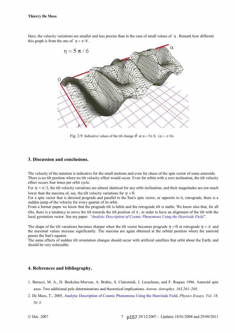
Thierry De Mees
© Dec. 2007 29/12/2007 - Updates 18/01/2008 and 29/09/2011 7
Here, the velocity variations are smaller and less precise than in the case of small values of . Remark how different this graph is from the one of /4 .
Fig. 2.9: Indicative values of the tilt change at 5 /6 (- /6). 3. Discussion and conclusions. The velocity of the nutation is indicative for the small motions and even for chaos of the spin vector of some asteroids. There is no tilt position where no tilt velocity effect would occur. Even for orbits with a zero inclination, the tilt velocity effect occurs four times per orbit cycle. For /2, the tilt velocity variations are almost identical for any orbit inclination, and their magnitudes are not much lower than the maxima of, say, the tilt velocity variations for . For a spin vector that is directed prograde and parallel to the Sun's spin vector, or opposite to it, retrograde, there is a sudden jump of the velocity for every quarter of its orbit. From a former paper we know that the prograde tilt is labile and the retrograde tilt is stable. We know also that, for all tilts, there is a tendency to move the tilt towards the tilt position of , in order to have an alignment of the tilt with the local gyrotation vector. See my paper: “Analytic Description of Cosmic Phenomena Using the Heaviside Field”. The shape of the tilt variations becomes sharper when the tilt vector becomes prograde or retrograde and the maximal values increase significantly. The maxima are again obtained at the orbital position where the asteroid passes the Sun's equator. The same effects of sudden tilt orientation changes should occur with artificial satellites that orbit about the Earth, and should be very noticeable. 4. References and bibliography. 1. Barucci, M. A., D. Bockelee-Morvan, A. Brahic, S. Clairemidi, J. Lecacheux, and F. Roques 1986. Asteroid spin
axes: Two additional pole determinations and theoretical implications. Astron. Astrophys. 163,261–268.
2. De Mees, T., 2005, Analytic Description of Cosmic Phenomena Using the Heaviside Field, Physics Essays, Vol. 18,
Nr 3.
p157

Thierry De Mees
© Dec. 2007 29/12/2007 - Updates 18/01/2008 and 29/09/2011 8
3. De Mees, T., 2005, Are Venus’ and Uranus’ tilt of natural origin?
4. De Mees, T., 2005, The Titius-Bode law shows a modified proto- gas-planets' sequence.
5. De Mees, T., 2007, The Gyro-Gravitational Spin Vector Torque Dynamics of Main Belt Asteroids in relationship
with their Tilt and their Orbital Inclination.
6. Einstein, A., 1916, Über die spezielle und die allgemeine Relativitätstheorie.
7. Erikson, A. 1999, The spin vector distribution of main belt asteroids. Bull. Am. Astron. Soc. 31,1112.
8. Erikson, A. 2000. The present distribution of asteroid spin vectors and its relevance to the origin and evolution of
main belt asteroids. DLR-Forschungsbericht 2000—37. DLR,Köln.
9. Feynman, Leighton, Sands, 1963, Feynman Lectures on Physics Vol 2.
10. Heaviside, O., A gravitational and electromagnetic Analogy, Part I, The Electrician, 31, 281-282 (1893)
11. Jefimenko, O., 1991, Causality, Electromagnetic Induction, and Gravitation, Electret Scientific, 2000.
12. Laskar, J., and P. Robutel, 1993, The chaotic obliquity of the planets, Nature 361, 608–612.
13. Skoglöv, E. 1999, Spin vector evolution for inner solar system asteroids. Planet. Space Sci. 47,11–22.
14. Skoglöv, E., P.Magnusson, and M. Dahlgren, 1996. Evolution of the obliquities for ten asteroids. Planet. Space Sci.
44,1177–1183.
15. Skoglöv, E., 2001, The Influence of the Orbital Evolution of Main Belt Asteroids, Icarus 160.
16. D. Vokrouhlický, D. Nesvorný, 2006, W.F. Bottke, Secular spin dynamics of inner main-belt asteroids, Icarus 184.
17. Zappalà, V., and Z. Knevžević 1984. Rotation axes of asteroids: Results for 14 objects, Icarus 59,435–455.
p158

Thierry De Mees
© Oct. 2011 13/10/2011 1
described by using the Maxwell Analogy for gravitation.
T. De Mees - thierrydm @ pandora.be
Abstract
Following to the two former papers “The Gyro-Gravitational Spin Vector Torque Dynamics of Main Belt Asteroids in relationship with their Tilt and their Orbital Inclination” and “Cyclic Tilt Spin Vector Variations of Main Belt Asteroids due to the Solar Gyro-Gravitation”, wherein we theoretically studied the tilt motions and variations of spinning asteroids, we continue the analysis with the study of the orbit anomalies of satellites. The equations for the fly-by of satellites near the Earth, or near planets in general are deduced. Keywords: Fly-by – satellite – planet – gravitation – gyrotation – prograde – retrograde – orbit. Method: Analytical. 1. Basic equations of the former papers.
In the former paper “The Gyro-Gravitational Spin Vector Torque Dynamics of Main Belt Asteroids in relationship with their Tilt and their Orbital Inclination”, a physical deduction is found for the motion and the variations of the tilt of asteroids. This deduction is based upon the Maxwell Analogy for Gravitation. As explained, the gravito-magnetic field of the Earth indeed influences the path of satellites because of their velocity, by the following equation, which is the analogue Lorentz force for gravity:
F ⇐ m ( g + v × Ω Ω Ω Ω ) (1.1)
Herein g is the gravity field vector of the Earth, ΩΩΩΩ its gravito-magnetic field vector (also called gyrotation), and m and v the mass and the velocity vector of the satellite. As explained the gravito-magnetic field vector is found out of the Earth’s data (see eq.(3.8.a) in that paper and eq.(1.2) below). The equations are totally valid for a spinning Earth that is surrounded by orbiting satellites. The Earth’s angular
velocity is ωωωω , its moment of inertia is I.
( )
3 2 2
3
2
r rG I
r c r
ωω
⋅ Ω = −
(1.2.a)
wherein for a sphere : (1.2.b) The value of the gyrotation can be found at each place in the universe, and is decreasing with the third power of the distance
r . The factor ω ω ω ω • r represents the scalar vector-product, and this value is zero at the equatorial level.
If we want to understand the accelerations of the satellites due to the second field, gyrotation, we need to know the vector
product v×Ω
in the vector equation (1.1) with the help of the vector equation (1.2). Therefore, we need some definitions of orbit angles, see fig.1.2.
Fig. 1.1 : A spinning sphere with radius R and rotation velocity ωωωω is generating a rotary gravitation field (or “gyrotation” field) ΩΩΩΩ at a distance r from the sphere's centre.
I m R= 2
52
Elliptical Fly-By and Expected Gyro-gravitational Orbit Accelerations
p159

Thierry De Mees
© Oct. 2011 13/10/2011 2
rY
X
Z
i
γ
α
βΩ
ω
In order to find the vector product v× Ω , we need to know the angle β in terms of the inclination i and the
position angle α , since the scalar vector-product of (1.2 a) is defined by cosrω β .
Therefore we notice that (see fig.1.2): sin cos sinzr r r iγ α= = (1.3.a)
And since sin cosγ β= , we get : cos cos siniβ α= (1.3.b) (1.3.c)
Hence, ( ) ( ) ( )( )2
3 2 2
3, , 0,0, , , cos sin
5x y z x y z
G m Rr r r r i
r c rω ω α Ω Ω Ω = −
(1.3.d)
wherein ( ) ( ), , cos cos ,sin ,cos sinx y zr r r r i iα α α= (1.3.e)
The equations (1.3) constitute the detailed vector formula of the equation (1.2). Remark that ω = ωearth .
2. Accelerations due to the Earth’s or planet’s spin.
In this paper, we will make abstraction of the satellite’s elliptic exact orbit shape, but the reader can implement that by defining an angle α0 that defines the location of the orbit’s pericenter. Then, by applying the angle α0 in the equation (1.3.e), the correct variability of the radius can be expressed. By using the classical velocity equations for elliptical orbits, defined by the angles α0 and α , the reader can find any primary velocity of the orbit. The analytical equations below are valid for α0 = 0. This means that the orbit’s pericenter coincides with the position of α = 0. They allow us to get graphical representations of the satellite accelerations due to the Earth’s gyrotation field. Rotation of coordinate system to the elliptical plane.
With (1.1), we find the accelerations v×Ω
due to gyrotation. In order to see more easily what really happens with a satellite, let us make a transform in the plane of the satellite’s orbit. More precisely a rotation of the system over the orbit inclination i. The coordinate system X’ Y’ Z’ is given by a clockwise rotation over the angle i :
( ) ( ), , cos sin , , sin cosX Y Z X i Z i Y X i Z i′ ′ ′ = + − + (2.1)
By doing this, we have put the satellite orbit in the X’ Y’ plane, and we can easily find the corresponding gyrotation
( ) ( ), , cos sin , , sin cosx y z x z y x zi i i i′ ′ ′Ω Ω Ω = Ω + Ω Ω − Ω + Ω (2.2)
Equation (2.2) is written in full in Appendix A.
Fig. 1.2 : Definition of the angles α and i . The orbital plane is defined by the orbital inclination i in relation to the X axis. The location of the asteroid inside the orbit is defined by the angle α . The equipotential line of the gyrotation ΩΩΩΩ through the asteroid has been shown as well.
p160
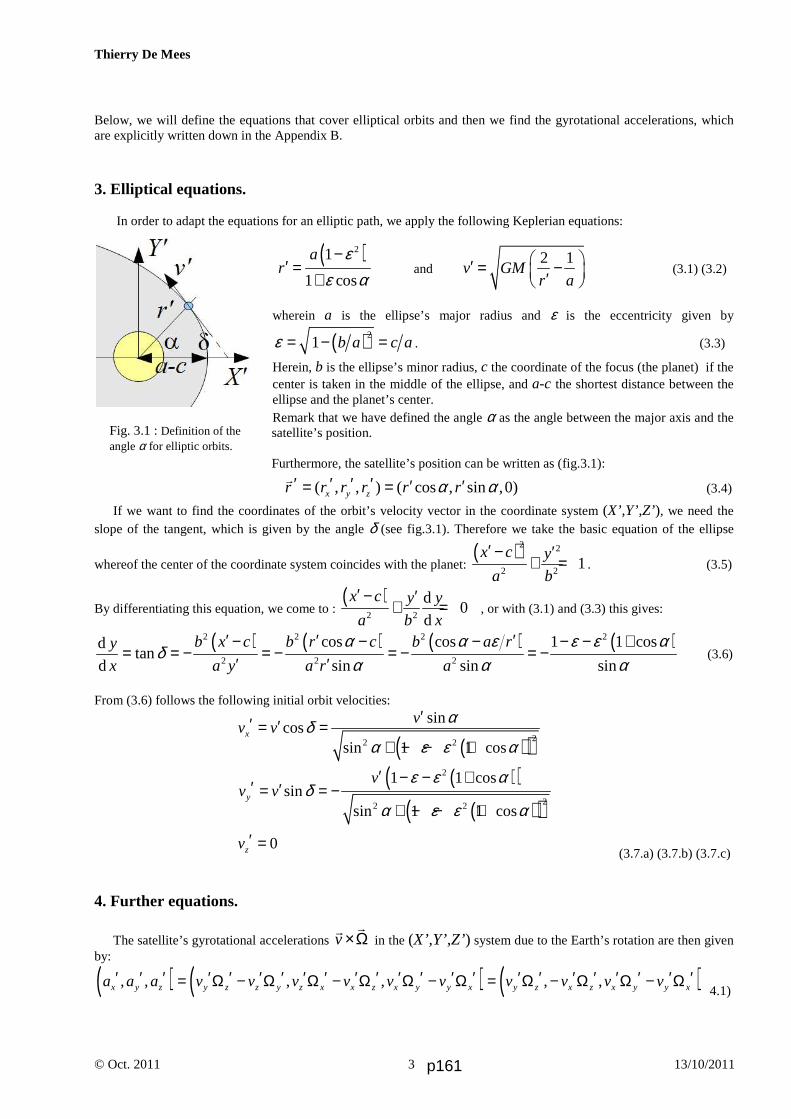
Thierry De Mees
© Oct. 2011 13/10/2011 3
Fig. 3.1 : Definition of the angle α for elliptic orbits.
Below, we will define the equations that cover elliptical orbits and then we find the gyrotational accelerations, which are explicitly written down in the Appendix B. 3. Elliptical equations.
In order to adapt the equations for an elliptic path, we apply the following Keplerian equations:
( )21
1 cos
ar
εε α
−′ =
+ and
2 1v GM
r a ′ = − ′
(3.1) (3.2)
wherein a is the ellipse’s major radius and ε is the eccentricity given by
( )21 b a c aε = − = . (3.3)
Herein, b is the ellipse’s minor radius, c the coordinate of the focus (the planet) if the center is taken in the middle of the ellipse, and a-c the shortest distance between the ellipse and the planet’s center. Remark that we have defined the angle α as the angle between the major axis and the satellite’s position. Furthermore, the satellite’s position can be written as (fig.3.1):
( , , ) ( cos , sin ,0)x y zr r r r r rα α′ ′ ′ ′ ′ ′= =
(3.4)
If we want to find the coordinates of the orbit’s velocity vector in the coordinate system (X’,Y’,Z’), we need the slope of the tangent, which is given by the angle δ (see fig.3.1). Therefore we take the basic equation of the ellipse
whereof the center of the coordinate system coincides with the planet: ( )2 2
2 21
x c y
a b
′ − ′+ = . (3.5)
By differentiating this equation, we come to : ( )
2 2
d0
d
x c y y
a b x
′ − ′+ = , or with (3.1) and (3.3) this gives:
( ) ( ) ( ) ( )2 2 2 2
2 2 2
cos cos 1 1 cosdtan
d sin sin sin
b x c b r c b a ry
x a y a r a
α α ε ε ε αδ
α α α′ ′ ′− − − − − +
= = − = − = − = −′ ′
(3.6)
From (3.6) follows the following initial orbit velocities:
( )( )22 2
sincos
sin 1 1 cosx
vv v
αδα ε ε α
′′ ′= =+ − − +
( )( )( )( )
2
22 2
1 1 cossin
sin 1 1 cosy
vv v
ε ε αδ
α ε ε α
′ − − +′ ′= = −+ − − +
0zv ′ =
(3.7.a) (3.7.b) (3.7.c)
4. Further equations.
The satellite’s gyrotational accelerations v×Ω
in the (X’,Y’,Z’) system due to the Earth’s rotation are then given by:
( ) ( ) ( ), , , , , ,x y z y z z y z x x z x y y x y z x z x y y xa a a v v v v v v v v v v′ ′ ′ ′ ′ ′ ′ ′ ′ ′ ′ ′ ′ ′ ′ ′ ′ ′ ′ ′ ′ ′ ′= Ω − Ω Ω − Ω Ω − Ω = Ω − Ω Ω − Ω 4.1)
p161

Thierry De Mees
© Oct. 2011 13/10/2011 4
Option 1 : Rotation of coordinate system to polar coordinates versus the planet.
What interests us are the values of the tangential and the radial accelerations versus the planet, and finally the accelerations that are perpendicular to the orbital plane. To see these accelerations, let us make a transform in the plane of the satellite’s orbit. More precisely a rotation of the system over the angle α. The coordinate system X” Y” Z” is given by a counter-clockwise rotation over the angle α :
( ) ( ), , cos sin , cos sin ,X Y Z X Y Y X Zα α α α′′ ′′ ′′ ′ ′ ′ ′ ′= + − (4.2)
Or, for the accelerations:
( ) ( ), , cos sin , cos sin ,x y z x y y x za a a a a a a aα α α α′′ ′′ ′′ ′ ′ ′ ′ ′= + −
Wherein we find the radial and the tangential accelerations (see fig.3.2):
( ) ( ), , , ,x y z r t za a a a a a′′ ′′ ′′ ′= (4.3)
Option 2 : Rotation of coordinate system to polar coordinates versus the orbital path.
Another interest thing are the values of the tangential and the radial accelerations to the orbital path, and finally the accelerations that are perpendicular to the orbital plane. To see these accelerations, let us make a transform in the plane of the satellite’s orbit. More precisely a rotation of the system over the angle π+δ (since δ is negative). The coordinate system X* Y* Z* is given by a counter-clockwise rotation over the angle α :
( ) ( )* * *, , sin cos , sin cos ,X Y Z X Y Y X Zδ δ δ δ′ ′ ′ ′ ′= − + − − (4.4)
Or, for the accelerations:
( ) ( )* * *, , sin cos , sin cos ,x y z x y y x za a a a a a a aδ δ δ δ′ ′ ′ ′ ′= − + − −
Wherein we find the radial and the tangential accelerations (see fig.3.2):
( ) ( )* * * * *, , , ,x y z r t za a a a a a′= (4.5)
When using the equations (3.7), the equation (4.5) can be found. 5. Graphical solutions.
The figures 5.1 and 5.2 show the values of the accelerations that satellites undergo by the equation (4.5), written in full by the equation (D.3.a). The tangential acceleration at
*, along the satellite’s path is zero, as confirmed by the equations in the Appendix D. In fig. 5.1 we show the radial gyrotational acceleration ar
* , which points to the Earth’s center, for the values of i and α
between -π and π.
Fig. 3.2. rotation of the coordinate system.
Fig. 3.3. rotation of the coordinate system.
p162

Thierry De Mees
© Oct. 2011 13/10/2011 5
The values of ar
* are zero for the orbital inclinations i that are multiples of π/4. The highest absolute values are found for inclinations i between-in these values, especially for α equal to 0. For α equal to π or -π, there is an attenuation due to the orbit’s eccentricity. For circular orbits, there is no attenuation.
In fig. 2.2 we show the gyrotational acceleration az*, scaled at 25%, which is perpendicular to the satellite’s orbital
plane, for the values of i and α between -π and π.
Fig.2.2: The gyrotational acceleration az* , perpendicular to the orbital plane, of satellites about the Earth, in relation to the
orbital inclination i and the orbital position α of the satellite. We took a/b = 2 and we had to scale az* to 25% compared
with ar*. The red line are the zero values for α and i. The values of i and α are between -π and π. A side view is also shown.
Fig.5.1: The radial gyrotational acceleration ar* of satellites about the Earth, in relation to the orbital
inclination i and the orbital position α of the satellite. We took a/b = 2. The red line are the zero values for α and i. The values of i and α are between -π and π.
p163

Thierry De Mees
© Oct. 2011 13/10/2011 6
The scales of the orbital inclination and the orbital position of the satellite are taken the same for both graphs. Here as well, there is an attenuation at α = π.
The highest values of az* are obtained when the orbital inclination is at π/2, when the orbit is perpendicular to the
Earth’s equator. The prograde value is double as large (in absolute value) as the retrograde one, and the width (action radius) is also larger. Prograde orbits always swivel towards equatorial orbits (i = 0) and retrograde orbits first swivel towards i = π/2 , then towards the planet’s equator (i = 0). The retrograde value is smaller due to the elliptic shape, which causes an attenuation. This is caused by the choice of an elliptic orbit whereof the pericenter is situated according to fig.1.2. 6. Discussion and conclusions : the swiveling process of inclined orbits.
We have calculated the satellite accelerations due to the Earth’s rotation. It is found that the values of ar*
(perpendicular to the orbital path) are zero for an orbital inclination i equal to π/2 and its multiples. The highest absolute values are found for an inclination i of π/4 and 3π/4, for α equal to 0. For α equal to π there is an attenuation due to the orbit’s eccentricity. For circular orbits, the value α at π equals that of α = 0 (in absolute values).
With the least satellite’s orbit inclination, away from the planet’s equator, an important radial acceleration occurs upon the satellites. At i = π/4 already, the acceleration ar
* comes to an absolute maximum around the pericenter. This explains why significant alterations of the satellites’ paths occurred near Saturn.
For specific fly-bys, the double integration of xa ′ and ya ′ over time gives the satellite’s extra displacement due to the
planet’s spin. The energy increase can be found from it as well. There is no gyrotational acceleration along the satellite’s path, since at
* is found to be zero. A vector product indeed cannot be oriented the same as one of the product’s components.
The strongest values for the acceleration az* (acceleration that is perpendicular to the orbital plane) are obtained for
the inclinations i that are perpendicular to the planet’s equatorial plane, at π/2. The orbital positions α where the highest absolute values are obtained, are zero. The maximal absolute values of az
* are significantly larger than those of ar
*. Prograde orbits always swivel towards equatorial orbits and retrograde orbits first swivel towards the poles first, then towards the planet’s equator. 7. References and bibliography. 1. Anderson, John D.; James K. Campbell, Michael Martin Nieto, 2007, The energy transfer process in planetary
flybys, New Astronomy 12 (5): 383–397, arXiv:astro-ph/0608087
2. Anderson, et. al. , 2008, Anomalous Orbital-Energy Changes Observed during Spacecraft Flybys of Earth, Phys.
Rev. Lett.
3. Barucci, M. A., D. Bockelee-Morvan, A. Brahic, S. Clairemidi, J. Lecacheux, and F. Roques, 1986. Asteroid spin
axes: Two additional pole determinations and theoretical implications. Astron. Astrophys. 163,261–268.
4. De Mees, T., 2005, Analytic Description of Cosmic Phenomena Using the Heaviside Field, Physics Essays, Vol.
18, Nr 3.
5. De Mees, T., 2007 – upd. 2011, Analytic The Gyro-Gravitational Spin Vector Torque Dynamics of Main Belt
Asteroids in relationship with their Tilt and their Orbital Inclination, General Science Journal.
6. De Mees, T., 2007 – upd. 2011, Cyclic Tilt Spin Vector Variations of Main Belt Asteroids due to the Solar Gyro-
Gravitation, General Science Journal.
7. Einstein, A., 1916, Über die spezielle und die allgemeine Relativitätstheorie.
8. Erikson, A. 1999, The spin vector distribution of main belt asteroids. Bull. Am. Astron. Soc. 31,1112.
p164
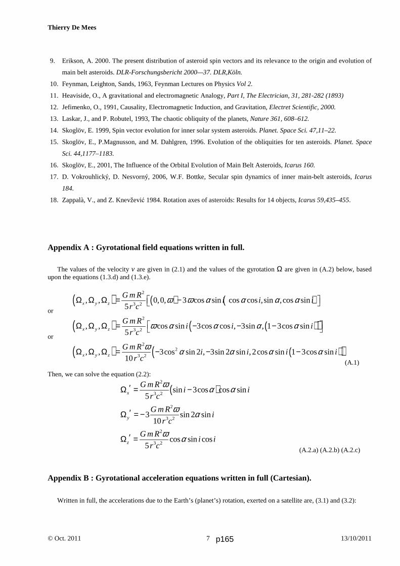
Thierry De Mees
© Oct. 2011 13/10/2011 7
9. Erikson, A. 2000. The present distribution of asteroid spin vectors and its relevance to the origin and evolution of
main belt asteroids. DLR-Forschungsbericht 2000—37. DLR,Köln.
10. Feynman, Leighton, Sands, 1963, Feynman Lectures on Physics Vol 2.
11. Heaviside, O., A gravitational and electromagnetic Analogy, Part I, The Electrician, 31, 281-282 (1893)
12. Jefimenko, O., 1991, Causality, Electromagnetic Induction, and Gravitation, Electret Scientific, 2000.
13. Laskar, J., and P. Robutel, 1993, The chaotic obliquity of the planets, Nature 361, 608–612.
14. Skoglöv, E. 1999, Spin vector evolution for inner solar system asteroids. Planet. Space Sci. 47,11–22.
15. Skoglöv, E., P.Magnusson, and M. Dahlgren, 1996. Evolution of the obliquities for ten asteroids. Planet. Space
Sci. 44,1177–1183.
16. Skoglöv, E., 2001, The Influence of the Orbital Evolution of Main Belt Asteroids, Icarus 160.
17. D. Vokrouhlický, D. Nesvorný, 2006, W.F. Bottke, Secular spin dynamics of inner main-belt asteroids, Icarus
184.
18. Zappalà, V., and Z. Knevžević 1984. Rotation axes of asteroids: Results for 14 objects, Icarus 59,435–455.
Appendix A : Gyrotational field equations written in full.
The values of the velocity v are given in (2.1) and the values of the gyrotation Ω are given in (A.2) below, based
upon the equations (1.3.d) and (1.3.e).
or ( ) ( ) ( )
2
3 2, , 0,0, 3 cos sin cos cos ,sin ,cos sin
5x y z
G m Ri i i
r cω ω α α α αΩ Ω Ω = −
or ( ) ( )( )
2
3 2, , cos sin 3cos cos , 3sin , 1 3cos sin
5x y z
G m Ri i i
r cω α α α α Ω Ω Ω = − − −
( ) ( )( )2
23 2
, , 3cos sin 2 , 3sin 2 sin ,2cos sin 1 3cos sin10x y z
G m Ri i i i
r c
ω α α α αΩ Ω Ω = − − −(A.1)
Then, we can solve the equation (2.2):
( )2
3 2sin 3cos cos sin
5x
G m Ri i
r c
ω α α′Ω = −
2
3 23 sin 2 sin
10y
G m Ri
r c
ω α′Ω = −
2
3 2cos sin cos
5z
G m Ri i
r c
ω α′Ω = (A.2.a) (A.2.b) (A.2.c)
Appendix B : Gyrotational acceleration equations written in full (Cartesian).
Written in full, the accelerations due to the Earth’s (planet’s) rotation, exerted on a satellite are, (3.1) and (3.2):
p165

Thierry De Mees
© Oct. 2011 13/10/2011 8
( )( )
( )( )( )( )
22
3 2 2 22 2
1 1 cos cos sin 22 1 cos1
10 1 sin 1 1 cosx
iG m R GMa
r c a
ε ε α αε αωε α ε ε α
− − ++′ = − − − + − − +
( )( ) ( )( )
2
3 2 2 22 2
2 1 cos sin 2 sin 21
20 1 sin 1 1 cosy
G m R GM ia
r c a
ε αω αε α ε ε α
+′ = − − − + − − +
( )( )
( )( )( )( )( )
2 22
3 2 2 22 2
1 1 cos sin 3cos 3sin2 1 cos1 cos sin
5 1 sin 1 1 cosz
iG m R GMa i
r c a
ε ε α α αε αω αε α ε ε α
− − + − −+′ = − − + − − +
(B.1.a) (B.1.b) (B.1.c) Appendix C : Gyrotational acceleration equations written in full (polar versus the planet).
Written in full, the accelerations due to the Earth’s (planet’s) rotation, exerted to a satellite are:
( )( )
( )( )( )( )
2 22
3 2 2 22 2
sin 1 1 cos cos2 1 cos1 sin 2 cos
10 1 sin 1 1 cosx r
G m R GMa a i
r c a
α ε ε α αε αω αε α ε ε α
− − − ++′′ = = − − + − − +
( )( )
( )( )( )( )
22
3 2 2 22 2
cos 1 1 cos2 1 cos1 sin 2 sin 2
20 1 sin 1 1 cosy t
G m R GMa a i
r c a
α ε ε αε αω αε α ε ε α
− − − ++′′ = = − − + − − +
( )( )
( )( )( )( )( )
2 22
3 2 2 22 2
1 1 cos sin 3cos 3sin2 1 cos1 cos sin
5 1 sin 1 1 cosz z
iG m R GMa a i
r c a
ε ε α α αε αω αε α ε ε α
− − + − −+′′ ′ = = − − + − − +
(C.1.a) (C.1.b) (C.1.c)
Appendix D : Gyrotational acceleration equations written in full (polar versus the orbit).
Written in full, the accelerations due to the Earth’s (planet’s) rotation, exerted to a satellite are:
( )( )
2* *
3 2 2
2 1 cos1 sin 2 cos
10 1x r
G m R GMa a i
r c a
ε αω αε
+ = = − − −
* 0y ta a= =
( )( )
( )( )( )( )( )
2 22*
3 2 2 22 2
1 1 cos sin 3cos 3sin2 1 cos1 cos sin
5 1 sin 1 1 cosz z
iG m R GMa a i
r c a
ε ε α α αε αω αε α ε ε α
− − + − −+′ = = − − + − − +
(D.1.a) (D.1.b) (D.1.c)
p166

7Interpreting the Cosmic Redshiftsfrom Quasars
The two next papers are related by the study of the redshift of light that comes from the limits of theuniverse.The observational data from astrophysicists is sometimes very unclear, and some interpretationssometimes are completely wrong because of a lack of available applicable physics. I start in the first paper to compare the angular momentum of a galaxy with its formed quasar. The quasars' redshifts and their matter-jets can be interpreted by basic physical assumptions and byGravitomagnetism, and compared with the related galaxy. This first paper should be seen as anattempt and as a draft for further studies.
If redshift is not workable to determine distance of light, maybe another way is useful: accordingGravitomagnetism, the distance should be dependent from the inverse square of the frequency.Let us discover the most secret parts of cosmology!
p167

Thierry De Mees
Quasar's Gyro-gravity Behavior, Luminosity and Redshift.
Described by using
the Maxwell Analogy theory.
T. De Mees - thierrydemees @ pandora.be
Abstract
The high redshift value of quasars is generally described by the Hubble constant, related to the Doppler-effect due
to the expansion of the universe. In this paper, we look closer to the part of the redshift that is caused by gyro-
gravitation, which is the analogue application of the electromagnetic Maxwell equations upon gravitation.
The result of our analysis explains the possibility of a high value difference between the quasar redshift and the
related galaxy redshift due to the quasar's rotation (spin). Moreover, we find results that are within the observed
redshifts, based only on the expected quasar-radius of a few light-weeks, without the artifact of an expanding
universe.
Key words : quasar, gravitation, luminosity, gyrotation, galaxy.
Method : analytic.
1. Pro Memore : Maxwell Analogy equations in short, symbols and basic equations.
The formulas (1.1) to (1.6) form a coherent set of equations, similar to the Maxwell equations. The electrical
charge q is substituted by the mass m, the magnetic field B by the Gyrotation ΩΩΩΩ , and the respective constants as
well are substituted (the gravitation acceleration is written as g and the universal gravitation constant as G =
(4π ζ)-1. We use sign ⇐ instead of = because the right hand of the equation induces the left hand. This sign ⇐
will be used when we want to insist on the induction property in the equation. F is the induced force, v the
velocity of a mass m with density ρ. The operator × symbolizes the cross product of vectors. Vectors are written
in bold.
F ⇐ m (g + v × ΩΩΩΩ ) (1.1)
∇∇∇∇ g ⇐ ρ / ζ (1.2)
c² ∇∇∇∇× ΩΩΩΩ ⇐ j / ζ + ∂g /∂ t (1.3)
div ΩΩΩΩ ≡ ∇ ∇ ∇ ∇ ΩΩΩΩ = 0 (1.4)
∇∇∇∇× g ⇐ – ∂ ΩΩΩΩ / ∂ t (1.5)
div j ⇐ – ∂ρ / ∂ t (1.6)
where j is the flow of mass through a surface.
All applications of the electromagnetism can from then on be applied on the gyrogravitation with caution. Also it
is possible to speak of gyrogravitation waves.
© June 2009 release June 20091 p168

Thierry De Mees
2. Rotation of galaxies and quasars.
Quasars are seen as the originator of galaxies. The jets of matter from surrounding nebulae or accretion discs are
projected at high speed from each side of the quasar rotation axis and form spinning nebulae. The projected matter
that is situated quite far from the quasar's both poles will hold up the new projected matter in order to form a kind
of spinning bar along the quasar's spinning axis, with at each end, a spinning knot, and in the middle the slowly
dying quasar.
2.1. Angular momentum of a galaxy.
When I have calculated the velocity of the stars in a galaxy, based on a certain simple mass distribution, I found a
simple relationship between the bulge's mass and radius, and the velocity of the stars.
In “A coherent dual vector field theory for gravitation”, I found the velocity of the stars in a disc galaxy as :
wherein Mo is 10 % of the total mass M and Ro is the radius of the bulge. (2.1)
The angular momentum of the galaxy can be found as follows: (2.2)
The velocity v is constant and corresponds to (2.1). The mass distribution
is supposed to be the quantity of the bulge's mass Mo every step of Ro .
This means that between every Ri and Ri+1 we find a mass Mo (see fig.
2.1). The inertial momentum of a ring shaped part of the disc is
(2.3)
at a position i in the bulge (see fig. 2.1). To fix the ideas, we take the galaxy's overall radius R = 10 Ro .
We find the angular momentum of the galaxy by making the sum of (2.2) by using (2.3).
Since R i Ri = + 1 0b g , we find L M R v i G M Ri
= + ==
∑0 00
9
03
01 55b g (2.4)
When we make the sum of (2.3) , we get I M R i M Ri
= + ==
∑0 02 2
0
9
0 021 385b g (2.5)
and since L I= ω , we find the average value for the galaxy's angular velocity ω g :
(2.6)
Or, in figures : ω g rad s= ⋅ −7 24 10 13. (2.7)
(Instead of the sums in (2.4) and (2.5) , we should have put integrations which would result in the quotient 50/333
instead of 55/385 . However, this doesn't make any difference in the general discussion).
For our Milky Way, we took the reasonable estimate of a bulge diameter of 10000 light years having a mass of 20
billion of solar masses.
© June 2009 release June 20092
vG MRR
2 0
0
=
∆ ∆ ∆L IvR
Ii
= =ω
Mo
Mo
Mo
0 1 2
h
Fig. 2.1. The disc galaxy after
collapsing of the orbits.
∆ ∆I R M R Mi i i= =2 20
ω g0
0
=55
385 3
G MR
p169

Thierry De Mees
2.2. Angular momentum and angular velocity of a quasar.
The mass and the angular momentum of both the galaxy and the corresponding quasar are of the same order
because there is a limited loss of mass in time.
We could consider a quasar as a sphere, but, due to my former work, I have found out that the shape should be a
torus. But since we speak of orders of magnitude, it doesn't change much anyway.
Thus, for the quasar, the same value of L is valid.
We can write, in general : L L M Rgalaxy quasar q q q= = 2ω (2.8)
Since the total mass remained the same : M Mq 0= 10 , (2.9)
we have to find out the other parameters.
The observation of quasars suggests that the radius of a quasar could be as small as a few light-weeks. Just to fix
an order of magnitude that is generally accepted (in fact even lower radii are supposed) we'll take a radius of 16
light-weeks, which is 1.45 ⋅ 1012 m.
We get now only two subordinated parameters left, the mass density and the mass velocity, which both are
interdependent.
A second important observation of stars resulted in the fact that the equatorial angular velocity is much slower
than the internal angular velocities. Since quasars have the shape of a torus (see my earlier paper “On the
geometry of rotary stars and black holes”) , we can in a first approximation also assume that the velocity of the
matter in the quasar is nearly constant.
Hence, assuming that the velocity is 10% of the speed of light : ω qq q
= =vR
cR10
(2.10)
We chose this velocity just as an example, because this is a free parameter in these calculations, and we will
calculate the corresponding density of the quasar. If the result is reasonable compared with the chosen mass'
velocity, we can form a basis for further research with the gyro-gravitation theory (or Maxwell Analogy for
Gravitation).
To the benefit of simple calculations that we do here to find out if the found density is of a credible order of
magnitude, we will assume that quasars are ideal fluids and that their density is equal over the whole object.
Let us write the moment of inertia of the quasar about its spin axis as : I M Rq q q= κ 2(2.11)
wherein κ is a figure of order zero (100) that depends on the exact shape of the torus.
Then I Rq q q= ′π κ κ ρ 5 wherein κ' also is a figure of order zero (100) that depends on the exact shape of the
torus and ρ is the constant density in the quasar.
And thus : d dI r rq q q q= ′π κ κ ρ 4(2.12.a.b)
For the angular momentum we find when using (2.10) and after integration to r , between zero and Rq :
L I c Rquasar q q q q= = ′ω π κ κ ρ1
84
(2.13)
So, when using (2.11) , knowing that the angular momenta of the quasar and the galaxy are equal, and when using
the integrated version of (2.4) -see the remark after equation (2.7)- :
© June 2009 release June 20093 p170

Thierry De Mees
ρπ κ κ π κ κ
qgalaxy
q
0 0
q
=′
=′
8 4004
3
4
L
c R
G M R
c R(2.14)
In figures, when assuming that κ = κ' = 1 , this gives : ρquasar3kg m= ⋅4 35 104. . (2.15)
3. The gamma-ray production of quasars.
It seems maybe strange that we have chosen a mass' velocity as large as 10% of the speed of light. However, the
observed large jets of quasars make us believe that the velocity should be high. Hereafter follows the relationship.
At the quasar's surface, the high speed of matter creates a huge inwards force due to the gyrotation force that is
given by the second part of the equation (here, it is written down for a ring-shaped object) :
(3.1)
The first part is the centrifugal force (inertia resistance), the third is the pure gravitation. The equation shows only
the force along the x-axis that is perpendicular to the spin axis. The angle α is the angle compared to the equator.
Equation (3.1) is taken from my paper “On the geometry of rotary stars and black holes”, equation (3.3) , wherein
the spherical inertial moment has been replaced by a ring-shaped inertial moment.
Below a certain value of α , the global acceleration ax will be directed inwards for an unlimited angular velocity,
provided that for the quasar's radius we have :
(3.2)
With the figures of chapter 2, we come indeed to the validity of (3.2) , what means that the quasar that would be
deducted from our galaxy would be compressed without exploding in a certain zone, which is defined by –35°16’
> α > 35°16’.
In the former chapter, we have chosen a quasar's radius that is of the order of magnitude of the generally observed
quasars, and which is small enough to maintain the quasar together spites the high rotation speed. Moreover we
have chosen a radius that -mechanically speaking- allowed matter to spin at very high speeds (instead of 10 % of
the speed of light, the actual speed might even be much higher) . So, we might wonder why the observed emission
of X-rays couldn't simply be due to matter that got disintegrated into gamma rays due to this high speed, on top of
the gamma rays from the jets. The large gyro-gravitational forces made that the redshifted gamma-rays became X-
rays to us.
Although there is no direct proof for this point of view, it is an interesting hypothesis because it makes fit together
quite a number of puzzle pieces.
The high luminosity of quasars can also be explained by this disintegration, provided that the light would be able
to escape. And we can check that. The quasar is indeed never a full black hole because we proved in “On the
geometry of rotary stars and black holes” that the maximal possible explosion-free zone is –35°16’ > α >35°16’. This means that light will escape outside this zone anyway.
Remark that the produced gamma-rays will not be mechanically bound with the quasar any more.
The non-explosion-free zone of the quasar is then the originator of mass losses that forms a nebula environment
around the quasar.
© June 2009 release June 20094
a RG m
RcG m
Rx = −−L
NMM
OQPP −ω α
α α2
2
2 21
1 3
2cos
sin cosc h
R G M cq q< 2 2c h
p171
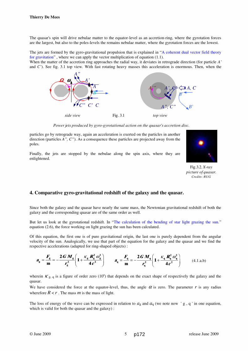
Thierry De Mees
The quasar's spin will drive nebulae matter to the equator-level as an accretion-ring, where the gyrotation forces
are the largest, but also to the poles-levels the remains nebulae matter, where the gyrotation forces are the lowest.
The jets are formed by the gyro-gravitational propulsion that is explained in “A coherent dual vector field theory
for gravitation” , where we can apply the vector multiplication of equation (1.1).
When the matter of the accretion ring approaches the radial way, it deviates in retrograde direction (for particle A’
and C’). See fig. 3.1 top view. With fast rotating heavy masses this acceleration is enormous. Then, when the
particles go by retrograde way, again an acceleration is exerted on the particles in another
direction (particles A”, C”). As a consequence these particles are projected away from the
poles.
Finally, the jets are stopped by the nebulae along the spin axis, where they are
enlightened.
4. Comparative gyro-gravitational redshift of the galaxy and the quasar.
Since both the galaxy and the quasar have nearly the same mass, the Newtonian gravitational redshift of both the
galaxy and the corresponding quasar are of the same order as well.
But let us look at the gyrotational redshift. In “The calculation of the bending of star light grazing the sun.”
equation (2.6), the force working on light grazing the sun has been calculated.
Of this equation, the first one is of pure gravitational origin, the last one is purely dependent from the angular
velocity of the sun. Analogically, we use that part of the equation for the galaxy and the quasar and we find the
respective accelerations (adapted for ring-shaped objects) :
(4.1.a.b)
wherein κ g, q is a figure of order zero (100) that depends on the exact shape of respectively the galaxy and the
quasar.
We have considered the force at the equator-level, thus, the angle α is zero. The parameter r is any radius
wherefore R < r . The mass m is the mass of light.
The loss of energy of the wave can be expressed in relation to ag and aq (we note now ' g , q ' in one equation,
which is valid for both the quasar and the galaxy) :
© June 2009 release June 20095
aF G M
r
R
cgg g
g
g g g
m= = − +
FHG
IKJ
21
42
2 2
2
κ ωa
F G M
r
R
cqq q
q
q q q
m= = − +
FHG
IKJ
21
42
2 2
2
κ ω
A’” A’, C’ A, C
B
A”, C” B’
side view Fig. 3.1 top view
Power jets produced by gyro-gyrotational action on the quasar's accretion disc.
A”
ΩΩΩΩ ω ω ω ω A’
A
B
C” C’ C
Fig.3.2. X-ray
picture of quasar.Credits :RUG
p172

Thierry De Mees
hh a
crd dυ
υ=
g,q
2 , thus :
dd
υ
υ=a
crg,q
2(4.2.a.b)
wherein υ is the frequency of the wave and h the Plank's constant.
Integrating this from Ro to infinity gives (υ 0 is the emitted frequency and υ the observed) :
d
dυ
υυ
υ
0
2z z=∞ a
cr
R
g,q
0
(4.3)
We can write (4.1.a.b) in terms of Mo and Ro , and knowing that Mg = Mq , Rg = 10 Ro , Rq = 3.1⋅10-5 Ro , we
see that all the right hand parameters of (4.1.a.b) are constants, except r . Let us call the group of constants 'A' ,
then we have after integration of (4.3) the equation for the redshift :
z eA c R
= − = −−υ
υ0 1 1
20e j
(4.4)
wherein A is the group of constants in (4.1.a.b) , respectively for the galaxy and the quasar:
A G MR
c= − +
FHG
IKJ2 1
4
2 2
2g,qg,q g,q g,qκ ω
(4.5)
For the galaxy, the gyro-gravitational redshift z is negligible, especially because the escaping light that has lost
energy by leaving the galaxy gains the energy back by entering the galaxy of the observer.
The final result for the galaxy's gyro-gravitational redshift is then by definition zero and that of the quasar (in this
example, for a quasar-radius of 16 weeks) is (with κ = κ' = 1 ) :
z = 0.06 (4.6)
This value is within the range of the observed redshifts for quasars. By taking the quasar's radius a little larger, the
redshift decreases.
5. Discussion and conclusions.
How foolish is the idea of matter that can have a velocity of 10 % of the speed of light? Is the plasma of super-
dense quasars behaving very differently to allow high densities? To what extend are the equatorial parts of the
quasar spinning slower than the inner part, as it is observed with the Sun and with stars, and what causes it? We
don't know the answer of these questions, but what we can assume is that the quasar's diameter is only a few light-
weeks, that the quasar's density and the spin velocity is very high, and that the origin of the strong jets is related to
the former parameters.
The excellent correlation between the quasar's diameter, the related galaxy's angular momentum and the gyro-
gravitational redshift is extraordinary, and allows to choose a reasonable set of remaining parameters of density
and spin velocity, which are interdependent.
The calculation didn't need any universe expansion theory, and here, the Ashmore redshift [4] has not been taken in
account.
© June 2009 release June 20096 p173
Thierry De Mees
6. References
1. De Mees : A coherent dual vector field theory for gravitation , General Science Journal, 2003.
2. De Mees : The calculation of the bending of star light grazing the sun , General Science Journal, 2004.
3. De Mees : On the geometry of rotary stars and black holes , General Science Journal, 2005.
4. Lyndon Ashmore : “Recoil Interaction Between Photons and The Electrons In The Plasma Of Intergalactic
Space Leading To The Hubble Constant And CMB”, March 2003.
http://www.lyndonashmore.com/
5. Gordon T. Richards et al. : “The SDSS Quasar Survey: Quasar Luminosity Function from Data Release Three.”,
2006, arXiv:astro-ph/0601434v2.
6. Hilton Ratcliffe : “A Review of Anomalous Redshift Data”, http://www.hiltonratcliffe.com, 2009.
7. H. Arp, C. Fulton : “A Cluster of High Redshift Quasars with Apparent Diameter 2.3 Degrees”,
arXiv:0802.1587v1, 2008.
8. H. Arp, C. Fulton : “The 2dF Redshift Survey II: UGC 8584 - Redshift Periodicity and Rings”,
arXiv:0803.2591v1, 2008.
© June 2009 release June 20097 p174
Thierry De Mees
Towards an Absolute Cosmic Distance Gauge by using Redshift Spectra from Light Fatigue.
Described by usingthe Maxwell Analogy for Gravitation.
T. De Mees - thierrydemees @ pandora.be
Abstract
Light is an electromagnetic wave with a dynamic mass, and with a zero rest mass. A fourth parameter isgyrotation, the second field of the Newtonian gravitation, discovered by using the Maxwell Analogy forGravitation. Here, we apply gyrotation for light. The dynamics analysis of the gyro-gravitation parameters forlight turns out in the possible existence of a very tiny light fatigue and a very tiny redshift as a direct consequence.This redshift however is frequency-dependent, unlike the other causes for redshift, as the Doppler effect, theAshmore effect, the gravitational redshift and the temperature redshift. The discovery of this quadraticallyfrequency-dependent redshift allows us to set up the basis for an universal cosmic distance measurement gauge.
Key words : gyrotation, gravitation, light fatigue.Method : analytic.
Index
1. Pro Memore : The Maxwell Analogy for gravitation: equations and symbols.
2. The mechanics and dynamics of light / The mechanics of light / The dynamics of light.
3. The dynamics of the dark energy in the presence of light / The gyro-gravitational description of a light wave /
Compression of a light wave / Depression of the light wave / Frequency-dependent redshift.
4. Discussion and conclusion.
5. References.
© Dec. 2009 release Dec. 20091
p175

c = E
ρ
E m c= 2
Thierry De Mees
1. Pro Memore : The Maxwell Analogy for gravitation: equations and symbols.
For the basics of the theory, I refer to : “A coherent double vector field theory for Gravitation”. The Maxwell Analogy laws for gravitation can be expressed in equations (1.1) up to (1.6) below.
In the 'gyro-gravitation theory' (or 'dual field gravitation theory' or 'Maxwell analogue gravitation theory', etc...),the electric charge is substituted by mass, the magnetic field by gyrotation, and the respective constants are also
substituted. The gravitation acceleration is written as g , the so-called second field or gyrotation field as Ω Ω Ω Ω (dimension [s-1]) and the universal gravitation constant is found as G-1 = 4π ζ , where G is the universal
gravitation constant and ζ the gravitation constant that is equivalent to the electrostatic constant ε . We use thesign ⇐ instead of = because the right-hand side of the equations causes the left-hand side. This sign ⇐ will beused when we want insist on the induction property in the equation. F is the resulting force, v the relative velocity
of the mass m with density ρ in the gravitational field. And j is the mass flow through a fictitious surface.
F ⇐ m ( g + v × Ω Ω Ω Ω ) (1.1)
∇∇∇∇ . g ⇐ ρ / ζ (1.2)
c² ∇∇∇∇× ΩΩΩΩ ⇐ j / ζ + ∂ g /∂ t (1.3)
div j ⇐ - ∂ρ / ∂ t (1.4)
div ΩΩΩΩ ≡ ∇∇∇∇. ΩΩΩΩ = 0 (1.5)
∇∇∇∇× g ⇐ - ∂ ΩΩΩΩ / ∂ t (1.6)
It is possible to speak of gyrogravitation waves with a transmission velocity c.
c2 = 1 / ( ζ τ ) (1.7) wherein τ = 4π G/c2. (1.8)
τ is the equivalent constant to the magnetic constant (permeability) µ .
2. The mechanics and dynamics of light.
2.1 The mechanics of light.
Light owns a dynamic mass, but not a rest mass. In that case, light must make use of a mass which isn't its own,but has to earn it from some medium. It borrows mass. The name we give that medium isn't important here, so letus call it dark energy. Light can then be seen as a compression of the medium itself, running at a velocity c, which is only dependentfrom the mass-density and the energy-density of the medium. The same equation for the wave velocity is thenfound, identical to the one of fluids:
(E is the energy-density, similar to an elasticity factor, ρ is the mass-density)
which is the same as saying that . The idea here is that the entity mass as well as the entity darkenergy are of the same kind. This gives a physical meaning to the famous equation, for light.
2.2 The dynamics of light.
Let us consider a light wave, traveling at a velocity c through the dark energy. A consequence of the propagatingmass wave in the weak gravitation field of the dark energy itself is that, when the wave propagates at a velocity c ,the compressed dark energy will almost instantly jump from a very low mass-density status to a very high mass-
density, and back again to the low density. This jump will result in the creation of a gyrotation field ΩΩΩΩ , that is
© Dec. 2009 release Dec. 20092 p176

Thierry De Mees
circular and perpendicular to the motion of the light, as explained in “A Coherent Dual Vector Field Theory forGravitation”.
In fig 2.1 is shown what happens in the weak gravitational field g , if a mass-flow (which here is directed towardsthe plane of the paper) travels in that field g .
A moving mass in a gravitation field will generate a second field (analogically toelectromagnetism) that is perpendicular to the gravitation field of the movingmass.
Fig. 2.1.
Since the sudden change of mass (pulse) occurs locally, the gyrotation field will be a local pulse as well. At acertain place, on the light's path the pulse first grows to a maximum, and decreases back to (almost) zero.
Fig. 2.2
A light wave, traveling in the positive x-axis' direction will generate locally anincreasing gyrotation field during thefirst half period of the wave. During thesecond half period, it will generate adecreasing gyrotation field.
For a certain location, this results in a increase of the gyrotation field during the first half period of the wave, and adecrease of the gyrotation field during the second half period of the wave.
3. The dynamics of the dark energy in the presence of light.
3.1 The gyro-gravitational description of a light wave.
Since the change of mass occurs locally as a pulse, the gyrotation field will be a local pulse as well. But if wefollow the wave, the value of the gyrotation pulse remains a constant, and in occurrence, it equals to the maximumvalue of the pulse.
While the gyrotation pulse travels with a velocity c , and the medium has a velocity zero (reference), the relativemedium velocity is indeed – c .Applying equation (1.1) results in the generation of a cylindrical gyrotation force which acts on the medium, asshown in fig.3.1.
© Dec. 2009 release Dec. 20093
ΩΩΩΩ m
g
.
y Ω
Ω Ω Ω Ω
c x
p177

Thierry De Mees
Fig.3.1.a. Fig.3.1.b.
A light wave travels with velocity c and creates an elementary cylindrical
gyrotation force FΩ on the medium's mass, towards the wave mass.
From equation (1.1) follows F mv= Ω with m V= ρ . Herein v is the velocity of the wave (in fact, the
speed of light: c) , m is its dynamical mass within the wave radius R , ρ is the density of the dark energy and Vis the volume of the uncompressed dark energy that is related to the electromagnetic wave.
3.2 Compression of a light wave.
The infinitesimal work to compress the light carrier, i.e. the dark energy is given by :
(3.1)
For a given cylinder with length λ and radius R , on which Ω acts , the total force is given by :
(3.2)
Here, R is the radius of the uncompressed dark energy volume that has to be taken in account for the light wave.The wave matter that flows through the dark energy at velocity c in a cylinder with radius R will be contracted bythe gyrotation that is created by this flux.
At the other hand, the infinitesimal radial displacement responds to d dr a t tg= , wherein ag is the
gravitational acceleration, wherefore we have the equation a cg = Ω . (3.3.a.b.)
This last equation follows from the physical origin of the speed of light in analogy with electromagnetism, wherewe use the electrical field E and the magnetic field B , wherefore E c B= .
The value of the time t is only half the period of the wave or t = 1
2υ . Hence, from (3.2.a) follows that :
(r ≥ R) (3.4)
© Dec. 2009 release Dec. 20094
yvrel = - c
Ω
FΩc x
d d dW E F r= = 2π
F c R R= π λ ρ 2 Ω
λ
r rcr
= =z d0 4
Ωυ
p178

Thierry De Mees
Since there is no gravitational source we can reduce equation (1.3) to c² ∇ ∇ ∇ ∇ × ΩΩΩΩ ⇐ j / ζ . The integratedequation, after application of the Stokes' theorem (see “A Coherent Dual Vector Field Theory for Gravitation”,equation (2.2)) , is :
(3.5)
For a circular path about the light packet, this gives : Ω = 2 2G m r c& c h (r ≥ R) (3.6)
wherein &m is the derivative of the mass to the time.
Now, we can say that for light waves, we have E mc= 2 and E h= υ .
At a certain place, the density of the dark energy changes to the compressed value of the light mass mhc
= υ2 .
Now, we know that the mass packet of a length λλλλ passes at a velocity of c. The variation of the mass packet over
time is then ∆ ∆m t . And the time ∆t correspondents to the period of the light packet which is the inverse of
the frequency : 1 υ .
Hence, it follows that the mass variation equals to : ∆∆mt
hc
= υ 2
2 (3.7)
Hence, we can rewrite (3.6) as : (r ≥ R) (3.8)
And the elimination of from (3.4) and (3.8) gives :
(r ≥ R) (3.9)
Since this elimination results in a right hand that is a constant for a given frequency υυυυ , we have to conclude that
r = R . Remark that the value of the radius R is only dependent from the frequency υυυυ .
Combining (3.8) and (3.9) gives also a frequency-dependent equation : (3.10)
Hence, (3.2) can be rewritten as follows, when filling in (3.9) and (3.10) :
(3.11)
and the integration of (3.1) becomes, for a work W over the wavelength λλλλ , since we know that R is a constant
for a given frequency υυυυ :
(3.12)
This is the work that is necessary for the compression of the light over a distance λλλλ .
3.3 Depression of the light wave.
The depression of the wave, when the light packet of length λλλλ passed by, should of course be the same value, butwith a minus sign, excepted a very tiny part, due to the fact that in the real world, we can expect that the elasticity
© Dec. 2009 release Dec. 20095
Ωz =d &l G m c4 2π
Ω = 2 2
4
G hr c
υ
rG h
c2
32= υ
Ω23
5
8= G hc
υ
F cG h
c= π λ ρ υ3 3 5
11
W G h cλ π λ ρ υ= −2 2 2 2 3 6
p179

Thierry De Mees
of the dark energy will show a very tiny energy loss. The value of this loss is unknown, and we represent it by the
loss factor (1- ε ε ε ε ) , wherein εεεε < 1 .
Hence, the energy gain by the depression is given by :
(3.13)
Unfortunately, we don't know how much will be lost. But anyway, the dark energy density isn't known either.
In order to do not confuse this with the tired light theories, which are cosmology theories, we call this effect “lightfatigue”. Light fatigue is a very small redshift effect that is only a fraction from the other causes of redshift.
3.4 Frequency-dependent redshift.
The equations (3.12) and (3.13) were found for a cylinder length of λλλλ , but for a distance dx between the emission
of the wave and its observation, we would get the following energy losses (we have put κκκκ in replacement of the
constants 2 1 2 2 2 6− −ε π ρb g G h c ) :
(3.14)
Hence, (3.15)
which, after integration gives the distance L between the emitter and the observer:
(3.16)
wherein the suffix o stands for observer and e for emitter.
Equation (3.16) shows that the redshift of the observed light will be non-linear, unlike the redshift that is causedby the recoil of hydrogen by the Mössbauer effect, unlike the gravitational redshift, unlike the redshift due to theDoppler effect and unlike the one due to temperature redshift.
An interesting consequence is that for a frequency spectrum of given isotopes, wherefore the values υυυυe are well
known, the distance L can be found by the spread of the observed frequency spectrum for these isotopes.When the linear redshifts have been subtracted, the remaining frequency-dependent spectrum will correspond toequation (3.15). It is true that the values of the dark energy's mass-density or its energy-density, as well as its inelastic part are notknown yet. An estimate can however been found by using the equation (3.15) for already known distances.
4. Discussion and conclusion.
If light fatigue, due to the slightly inelastic dark energy, can be observed, it has to be quadratically frequency-dependent. The possible presence of a quadratic colour shift for a very distant object could result in the finding ofthe real distance of that object to us. Other redshifts are frequency-invariant, such as the gravitational analogy forthe Compton effect (Zwicky) or Mössbauer redshift (L.Ashmore) , the gravitational redshift (Einstein) , Dopplerredshift (Doppler) and the temperature redshift (J.García). After subtraction of the frequency-invariant redshifts, asa whole, the remaining small redshift can appear to be quadratic. If so, no other know effect than the light fatigue
© Dec. 2009 release Dec. 20096
Lo e
= −FHG
IKJ
1
2
1 12 2κ υ υ
− = − −W G h cλ ε π λ ρ υ2 2 2 2 3 6
d d dW h x= =υ κ υ 3
dd
υυ
κυ
υ
30e
o
xL
z z=
p180

Thierry De Mees
will explain it. After a number of such observations, a relative distance scale can then be created in order to find
the loss factor (1- ε ε ε ε ) .
5. References.
1. Nobili S. , et al. (The Supernova Cosmology Project) : Constraining Dust and Color Variations of High-z SNe
Using NICMOS on the Hubble Space Telescope, 2009, ApJ, 700, 1415, arXiv:0906.4318.
2. Barbary K., et al., (Supernova Cosmology Project) : Discovery of an Unusual Optical Transient with the Hubble
Space Telescope 2009, ApJ, 690, 1358, arXiv:0809.1648
3. García J., Another Explanation of the Cosmological Redshift, 2009, General Science Journal.
4. Ashmore L., Recoil Interaction Between Photons and The Electrons In The Plasma Of Intergalactic Space
Leading To The Hubble Constant And CMB, March 2003, updated August 2004.
5. Zwicky, On the red shift of spectral lines through interstellar space, 1929, Proc. Nat. Acad. Sci., 15, 773-779.
6. De Mees, T., A coherent double vector field theory for Gravitation, 2003, General Science Journal.
7. Feynman, Leighton, Sands, 1963, Feynman Lectures on Physics Vol 2.
8. Heaviside, O., A gravitational and electromagnetic Analogy, Part I, The Electrician, 31, 281-282 (1893).
9. Jefimenko, O., 1991, Causality, Electromagnetic Induction, and Gravitation, (Electret Scientific, 2000).
© Dec. 2009 release Dec. 20097 p181

8The Coriolis Gravity Theory
When I tried to understand how Solar gravitons (that I expect be be a kind of electromagneticwaves) could transfer the forces of gravity, I discovered a physical law that relates the Sun's masswith its spin velocity. Only a few universal constants completed the relationship.This relationship allowed me to imagine how the escaped gravitons could interact with matter andobtain an attraction. It appeared to be nothing more but a Coriolis Effect! This simple CoriolisEffect explains attraction, repulsion and the inertia of matter! The first paper of this chapter relatesthis story.I explain in the second paper why the Earth expands under the influence of the Earth's spin, and inthe next paper I realize that the Gravitational Constant rather than the mass is changing when theearth expands. The stars' life cycle is an excellent evidence for example.In my fourth paper, I suggest that the mainstream concept of the Earth's inner core might be wrong.Two reasons are available to prefer a compression-free inner core.Finally, my fifth paper proves that although the Coriolis Gravity provides as many repel asattraction particles, nevertheless all heavenly bodies get a majority of attractive interactions.Discover now this theory that will open a totally new world in the next future!
p182
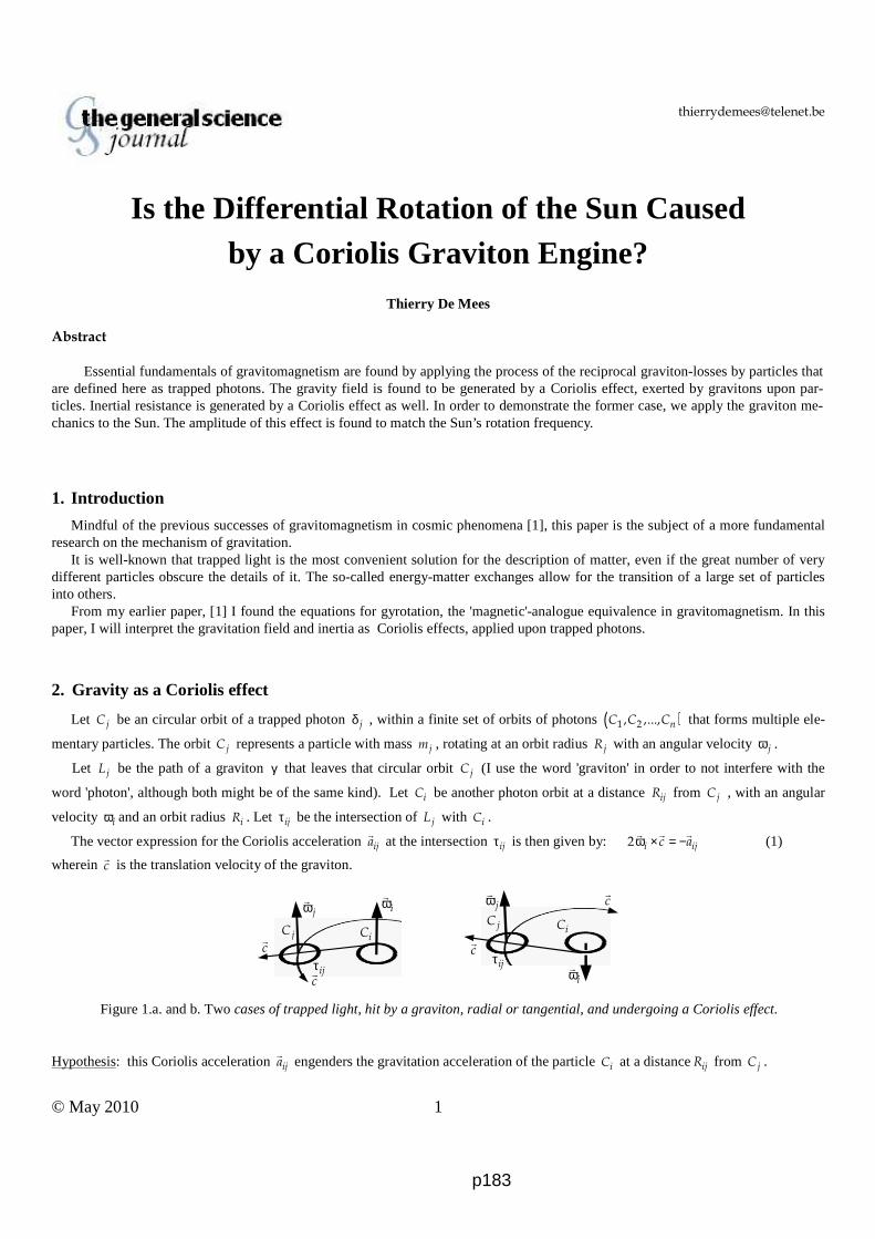
© May 2010 1
Is the Differential Rotation of the Sun Caused by a Coriolis Graviton Engine?
Thierry De Mees
Abstract
Essential fundamentals of gravitomagnetism are found by applying the process of the reciprocal graviton-losses by particles that are defined here as trapped photons. The gravity field is found to be generated by a Coriolis effect, exerted by gravitons upon par-ticles. Inertial resistance is generated by a Coriolis effect as well. In order to demonstrate the former case, we apply the graviton me-chanics to the Sun. The amplitude of this effect is found to match the Sun’s rotation frequency.
1. Introduction
Mindful of the previous successes of gravitomagnetism in cosmic phenomena [1], this paper is the subject of a more fundamental research on the mechanism of gravitation.
It is well-known that trapped light is the most convenient solution for the description of matter, even if the great number of very different particles obscure the details of it. The so-called energy-matter exchanges allow for the transition of a large set of particles into others.
From my earlier paper, [1] I found the equations for gyrotation, the 'magnetic'-analogue equivalence in gravitomagnetism. In this paper, I will interpret the gravitation field and inertia as Coriolis effects, applied upon trapped photons.
2. Gravity as a Coriolis effect
Let jC be an circular orbit of a trapped photon δ j , within a finite set of orbits of photons ( )1 2, ,..., nC C C that forms multiple ele-
mentary particles. The orbit jC represents a particle with mass jm , rotating at an orbit radius jR with an angular velocity jω .
Let jL be the path of a graviton γ that leaves that circular orbit jC (I use the word 'graviton' in order to not interfere with the
word 'photon', although both might be of the same kind). Let iC be another photon orbit at a distance ijR from jC , with an angular
velocity ωi and an orbit radius iR . Let τij be the intersection of jL with iC .
The vector expression for the Coriolis acceleration ija
at the intersection τij is then given by: 2 i ijc aω × = −
(1)
wherein c
is the translation velocity of the graviton.
Figure 1.a. and b. Two cases of trapped light, hit by a graviton, radial or tangential, and undergoing a Coriolis effect.
Hypothesis: this Coriolis acceleration ija
engenders the gravitation acceleration of the particle iC at a distanceijR from jC .
c
jω
iω
jC iC
ijτ
jω
iω
ijτ
jC iC
c
c
c
p183

© May 2010 2
The right hand of Eq. (1) is equal to the corresponding gravity acceleration, produced by the diluted fraction iGm of gravitons that
leave the circular photon orbit, in tangential or perpendicular directions. The gravitational acceleration flux in a point τij at a distance
ijR will be : 2i ijGm R− (2)
The total possible number of intersections τij is then given by ( )2 i iR Rπ . Hence, from Eq. (1) and (2) follows, in totality :
2
2
2
ii
ij
Gm
cR
πω = or
22
ii
ij
Gm
cRυ = (3)
wherein iυ is the according rotation frequency.
It was showed [1] that the mutual gyrotation orientations of nested particles in a rotating object, similar as jω
and iω
in figure
1.a., have like rotation orientations, due to the like-oriented gyrotation fields. However, particles that are apart from the object always get opposite spin orientations, like jω
and iω
in figure 1.b.
3. Inertia as a Coriolis effect
A direct consequence of regarding matter as trapped light is the interpretation of the mechanism of inertia. Also this mechanism is ruled by the Coriolis effect.
Let the trapped photon δ j be accelerated by a force in a certain direction, as shown in figure 2 and the photon paths will cross in
1jjτ and 2jjτ .
Figure 2. Trapped light under a force F
undergoes a Coriolis effect that is oriented in opposite direction.
There are six possible orientations of jω
(like the sides of a dice) whereof four result in the same orientation of the Coriolis accele-
ration 2jj ja c− = ω , and two of them that have a screwing shape (right of left screwing) don’t undergo any Coriolis effect at all.
4. Derivation of the Sun’s Rotation Equation
It will be shown below that Eq. (3), when applied to the Sun as a whole, gets a special meaning, due to the like orientation of par-ticles by the Sun’s rotation.
Since the gravitons are leaving the Sun in radial or tangential way, or any situation between-in, there is a net gravitational and rota-tional effect.
Hence, when applying Eq. (3) for gravitons that leave the Sun along the equator, we find:
Suneq 2
eq2
Gm
cRυ = (4)
Herein : G = 6.67x10⁻¹¹ m3 kg-1 s-2, c = 3.00x10⁸ m s-1 and for the Sun, Sunm = 1.98x1030 kg
eqR = 6.96x10⁸ m.
What I suggest here, is that the Sun’s angular velocity might be defined, due to a law of nature, by its gravitational properties. By
applying the figures above, this can immediately be checked. However, when it comes to the entrainment of matter by gravitons, a minimum of viscosity is required. The Dalsgaard model for
the solar density [3] shows a hyperbolic-like function, whereof the asymptotes intersect at about 0.98eqR : at first, there occurs a very
jC
jω
,F v
c
1jjτ
2jjτ
c
c
p184

© May 2010 3
quick density increase from 10-6 g/cm³ at eqR until 10-2 g/cm³ at nearly 0.95eqR and next a slow, almost linear density increase until
1.5x10² g/cm³ at the Sun’s center. On the other hand, S. Korzennik et al. [2] found that the highest value of the Sun’s rotation is lo-cated at about 0.94eqR , where the corresponding density is 10-2 g/cm³.
When applying Eq. (4) by using a corrected radius, somewhere between 0.98 and 0.94eqR , and when assuming that the total mass
may be kept alike, the result for the Sun’s rotation frequency eqυ is somewhere between 474 and 515 nHz, or a corresponding side-
real period between 24.44 and 22.49 days, which is very close to the measured Sun’s sidereal period of 24.47 days at the equatorial photosphere [2]. This result suggests that the equatorial disc of the Sun maintains and controls the rotation frequency of the Sun ever since the Sun started to rotate in some initial direction.
5. Derivation of the Sun’s Differential Rotation Equation
When a graviton quits the Sun at any latitude α , it will cause an acceleration as well, based on Eq. (4) , but whereby the spin ω will be inclined at an angle α (the equator is 0 rad) and whereby the radius eqR remains to same for all latitudes.
In a first approach, I reason as follows. The average direction between the Sun’s equatorial, graviton-induced spin, name it eqω ,
and the inclined spin, name it αω , is 2α . The value of αω should, in addition, be reduced by the cosine of 2α towards the rotation
axis because we only observe the component at the angle 2π .
Hence ( )eq cos 2αω = ω α (5)
This result is a raw equation for the differential rotation under the effect of gravitons but it doesn’t indeed take into account the centrifugal flow inside the Sun’s Convection Zone. This flow engenders a Coriolis effect up to the surface which attenuates the angu-lar velocity, especially in a range around the angle of 4π . It could be possible to extract a semi-empiric equation from Eq. (5) that
takes in account this motion, but this is not the prime purpose of this paper.
6. Discussion
The parity of the Coriolis acceleration with the Sun’s gravity acceleration, under the action of escaping gravitons, is remarkable. Gravitons at any latitude produce the same rotation value, which, combined with the global spin of the Sun, result in a differential ro-tation. The equator is the place where gravitons propel the Sun at the largest resulting velocity.
According to S. Korzennik et al. [2] , the measured differential rotation at the solar surface shows a wide range of rotation frequen-cies between nearly 337 nHz (rotation period of 34.3 days at the poles) and 473 nHz (rotation period of 24.47 days at the equator). With Eq. (5) we got a raw equation, without solar convection corrections, of the expected differential rotations at places, other than at the equator. For example, the calculated result –by using 0.98 eqR and without further corrections– for the poles is 34.56 days, which
comply very well with the measured rotation period of 34.3 days. The expression “Graviton Engine” follows from the mechanical Coriolis-process that is at the origin of Eq. (4).
7. Conclusion
Our Sun seems to behave like a giant particle whereof any place on the surface is propelled by gravitons that quit the Sun at a speed c . Its motion may confirm our gravitomagnetic interaction-model between particles, shaped as circular trapped light, wherein the Coriolis effect by gravitons generates gravitation. Other latitudes on the Sun’s surface, where the same process occur, directly con-tribute to the measured differential rotation.
8. References
[ 1 ] De Mees T., “Analytic Description of Cosmic Phenomena Using the Heaviside Field”, Physics Essays, Vol. 18, No. 3 (2005). [ 2 ] Korzennik, S. et al., ”Internal rotation and dynamics of the Sun from GONG data”, Kluwer, 1997IAUS..181..211K (1997). [ 3 ] NASA/Marshall Solar Physics". Solarscience.msfc.nasa.gov. 2007-01-18. http://solarscience.msfc.nasa.gov/interior.shtml.
p185
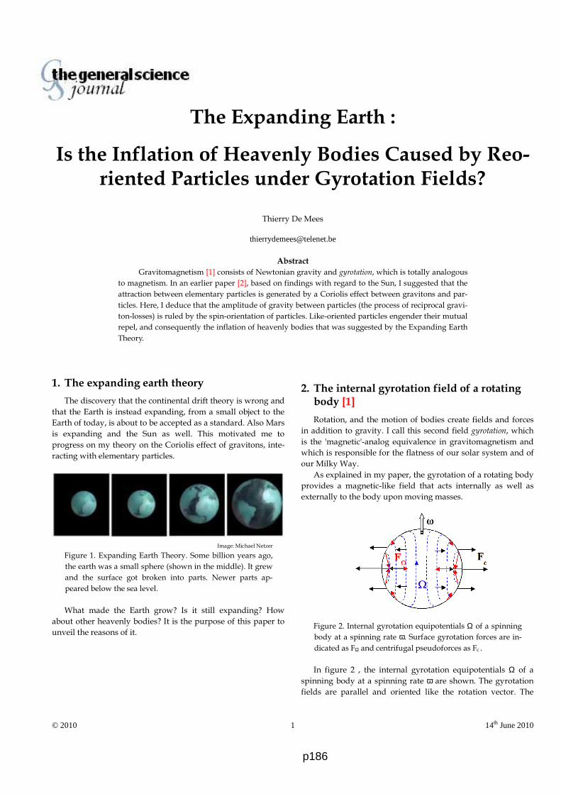
Thierry De Mees
© 2010 1 14th June 2010
The Expanding Earth :
Is the Inflation of Heavenly Bodies Caused by Reo-riented Particles under Gyrotation Fields?
Thierry De Mees
Abstract
Gravitomagnetism [1] consists of Newtonian gravity and gyrotation, which is totally analogous
to magnetism. In an earlier paper [2], based on findings with regard to the Sun, I suggested that the
attraction between elementary particles is generated by a Coriolis effect between gravitons and par-
ticles. Here, I deduce that the amplitude of gravity between particles (the process of reciprocal gravi-
ton-losses) is ruled by the spin-orientation of particles. Like-oriented particles engender their mutual
repel, and consequently the inflation of heavenly bodies that was suggested by the Expanding Earth
Theory.
1. The expanding earth theory
The discovery that the continental drift theory is wrong and
that the Earth is instead expanding, from a small object to the
Earth of today, is about to be accepted as a standard. Also Mars
is expanding and the Sun as well. This motivated me to
progress on my theory on the Coriolis effect of gravitons, inte-
racting with elementary particles.
Image: Michael Netzer
Figure 1. Expanding Earth Theory. Some billion years ago,
the earth was a small sphere (shown in the middle). It grew
and the surface got broken into parts. Newer parts ap-
peared below the sea level.
What made the Earth grow? Is it still expanding? How
about other heavenly bodies? It is the purpose of this paper to
unveil the reasons of it.
2. The internal gyrotation field of a rotating body [1]
Rotation, and the motion of bodies create fields and forces
in addition to gravity. I call this second field gyrotation, which
is the 'magnetic'-analog equivalence in gravitomagnetism and
which is responsible for the flatness of our solar system and of
our Milky Way.
As explained in my paper, the gyrotation of a rotating body
provides a magnetic-like field that acts internally as well as
externally to the body upon moving masses.
Figure 2. Internal gyrotation equipotentials Ω of a spinning body at a spinning rate ω. Surface gyrotation forces are in-dicated as FΩ and centrifugal pseudoforces as Fc .
In figure 2 , the internal gyrotation equipotentials Ω of a spinning body at a spinning rate ω are shown. The gyrotation fields are parallel and oriented like the rotation vector. The
p186
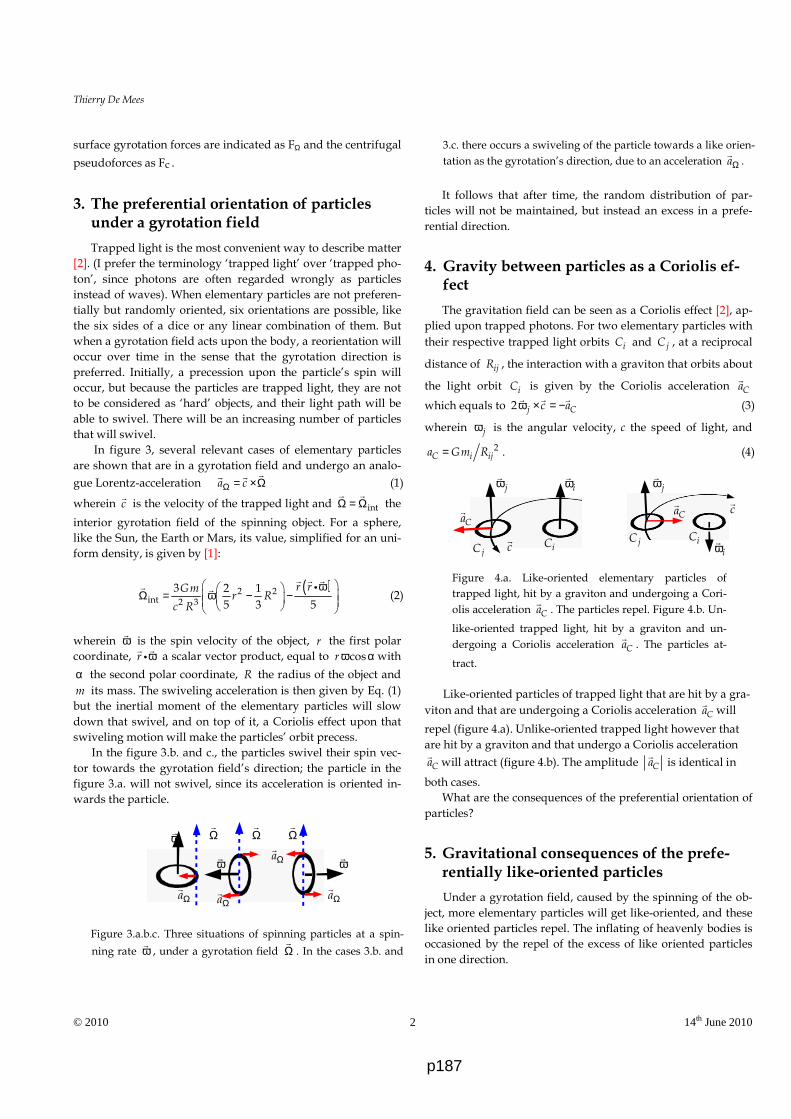
Thierry De Mees
© 2010 2 14th June 2010
surface gyrotation forces are indicated as FΩ and the centrifugal
pseudoforces as Fc .
3. The preferential orientation of particles under a gyrotation field
Trapped light is the most convenient way to describe matter
[2]. (I prefer the terminology ‘trapped light’ over ‘trapped pho-
ton’, since photons are often regarded wrongly as particles
instead of waves). When elementary particles are not preferen-
tially but randomly oriented, six orientations are possible, like
the six sides of a dice or any linear combination of them. But
when a gyrotation field acts upon the body, a reorientation will
occur over time in the sense that the gyrotation direction is
preferred. Initially, a precession upon the particle’s spin will
occur, but because the particles are trapped light, they are not
to be considered as ‘hard’ objects, and their light path will be
able to swivel. There will be an increasing number of particles
that will swivel.
In figure 3, several relevant cases of elementary particles
are shown that are in a gyrotation field and undergo an analo-
gue Lorentz-acceleration a cΩ = ×Ω
(1)
wherein c
is the velocity of the trapped light and intΩ = Ω
the
interior gyrotation field of the spinning object. For a sphere,
like the Sun, the Earth or Mars, its value, simplified for an uni-
form density, is given by [1]:
( )2 2
int 2 3
3 2 1
5 3 5
r rGmr R
c R
ω Ω = ω − −
i
(2)
wherein ω
is the spin velocity of the object, r the first polar
coordinate, r ω
i a scalar vector product, equal to cosrω α with
α the second polar coordinate, R the radius of the object and
m its mass. The swiveling acceleration is then given by Eq. (1)
but the inertial moment of the elementary particles will slow
down that swivel, and on top of it, a Coriolis effect upon that
swiveling motion will make the particles’ orbit precess.
In the figure 3.b. and c., the particles swivel their spin vec-
tor towards the gyrotation field’s direction; the particle in the
figure 3.a. will not swivel, since its acceleration is oriented in-
wards the particle.
Figure 3.a.b.c. Three situations of spinning particles at a spin-
ning rate ω
, under a gyrotation field Ω
. In the cases 3.b. and
3.c. there occurs a swiveling of the particle towards a like orien-
tation as the gyrotation’s direction, due to an acceleration aΩ
.
It follows that after time, the random distribution of par-
ticles will not be maintained, but instead an excess in a prefe-
rential direction.
4. Gravity between particles as a Coriolis ef-fect
The gravitation field can be seen as a Coriolis effect [2], ap-
plied upon trapped photons. For two elementary particles with
their respective trapped light orbits iC and jC , at a reciprocal
distance of ijR , the interaction with a graviton that orbits about
the light orbit iC is given by the Coriolis acceleration Ca
which equals to 2 j Cc aω × = −
(3)
wherein jω is the angular velocity, c the speed of light, and
2C i ija Gm R= . (4)
Figure 4.a. Like-oriented elementary particles of
trapped light, hit by a graviton and undergoing a Cori-
olis acceleration Ca
. The particles repel. Figure 4.b. Un-
like-oriented trapped light, hit by a graviton and un-
dergoing a Coriolis acceleration Ca
. The particles at-
tract.
Like-oriented particles of trapped light that are hit by a gra-
viton and that are undergoing a Coriolis acceleration Ca
will
repel (figure 4.a). Unlike-oriented trapped light however that
are hit by a graviton and that undergo a Coriolis acceleration
Ca
will attract (figure 4.b). The amplitude Ca
is identical in
both cases.
What are the consequences of the preferential orientation of
particles?
5. Gravitational consequences of the prefe-rentially like-oriented particles
Under a gyrotation field, caused by the spinning of the ob-
ject, more elementary particles will get like-oriented, and these
like oriented particles repel. The inflating of heavenly bodies is
occasioned by the repel of the excess of like oriented particles
in one direction.
c
jω
iω
jC iC
ω
ω
ω
Ω
Ω
Ω
aΩ
aΩ
aΩ
aΩ
Ca
jω
Ca
c
iωjC iC
p187

Thierry De Mees
© 2010 3 14th June 2010
Let's go over the main features of like and unlike spinning
elementary particles:
1° Gravity between elementary particles can be an attrac-
tion as well as a repel.
2° Consequently, the ‘universal’ gravitation constant isn’t
universal at all but ‘local’ and its value depends from the de-
gree of like or unlike orientations of particles in the bodies.
3° Rotating (spinning) bodies get steadily more like-
oriented particles and consequently, steadily higher values of
the ‘local’ gravitation constant.
4° The gravity of an object, containing ideally random-
oriented particles doesn’t have any global gravitational effect!
In other words, if there is no preferential orientation of the par-
ticles, no global gravitational attraction (or repel) will occur!
5° The parameters of the gravitational attraction and repel
of bodies are their masses (as far as they can be regarded as
absolute values), their distance and their excess quantity of like
oriented particles (also expressible by the ‘local’ gravitation
constant of each of the bodies, as vectors).
6° Rotating (spinning) bodies inflate.
6. Discussion
The Sun, the earth, Mars and all the planets that spin or that
are influenced by the spinning Sun, undergo a transformation
inside. The rotation of the bodies generate a gyrotation of the
same orientation inside the bodies. Due to the Coriolis affect,
like spinning elementary particles get repelled and unlike at-
tracted.
But, let us analyze the external gyrotation of spinning bo-
dies, as a bonus.
Figure 5. A rotating body also provides an external gyrota-
tion Ω that has an inverse orientation of the body’s rotation. Every orbiting body gets that gyrotation field working on it,
which orient the elementary particles to it, with time. At-
traction of the body occur. Surface gyrotation forces are in-
dicated as FΩ and centrifugal pseudoforces as Fc .
Spinning bodies indeed procure a gyrotation field that is
the inverse of the body’s rotation, and every orbiting object will
undergo that gyrotation field by orientating the particles prefe-
rentially in the inverse direction (see figure 5). Let the large
body be the Sun and the small one the Earth. Since the excess of
orientation of the Sun’s particles is opposite to the one of the
Earth, the gravitons will cause attraction. On the long term, the
Earth’s rotation will slow down, the more that the earth ex-
pands, but the number of like-oriented particles with the Sun
will increase at a slower rate as well, and cause a slower widen-
ing of the Earth’s orbit with time.
One could wonder if the objects on Earth wouldn’t be
changing their weight, depending from the orientation of the
object. Would an upside-down object be repelled by the Earth?
No, because the elementary particles conserve their orientation,
whatever the bodies orientation is. And the Earth’s gyrotation
field is more or less oriented likewise over the Earth, opposite
to the Earth’s rotation, which results in a comparably attraction
force all over the world.
7. Conclusion
The expanding Earth has an explanation that is consistent
with gravitomagnetism and with (what I would call) the Cori-
olis Gravity Theory [2]. The like spin of elementary particles
cause gravitational repel and the unlike spin, attraction. Gyro-
tation fields, induced from rotation, orient these spins preferen-
tially likewise with the body’s rotation, which results in the
repel inside the body, and so, its expansion. The consequence
of it is that gravity doesn’t always mean attraction, because it
depends from the excess of orientation of particles in specific
directions. Gravity can be repulsive and attractive. The gravita-
tion constant is not a constant at all but should rather be seen
as a fraction of a mass one (when masses are regarded as abso-
lute entities) that interferes with the fraction of a mass two. It is
then probable that the supposed ‘absolute’ mass of some pla-
nets is different of what has been supposed until now.
References
[ 1 ] De Mees, T., “Analytic Description of Cosmic Phenomena
Using the Heaviside Field”, Physics Essays, Vol. 18, No. 3
(2005).
[ 2 ] De Mees, T., “Is the Differential Rotation of the Sun Caused
by a Graviton Engine”, Proceedings of the NPA, (2010).
p188
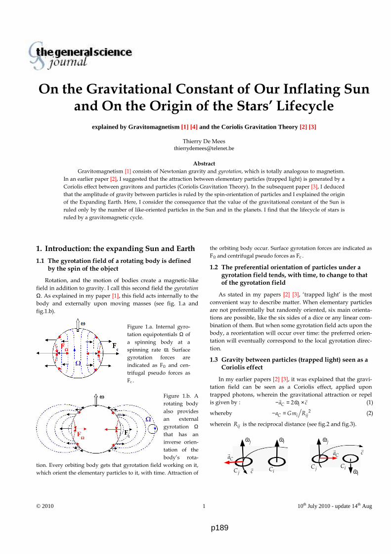
Thierry De Mees
© 2010 1 10th July 2010 - update 14th Aug
On the Gravitational Constant of Our Inflating Sun and On the Origin of the Stars’ Lifecycle
explained by Gravitomagnetism [1] [4] and the Coriolis Gravitation Theory [2] [3]
Thierry De Mees [email protected]
Abstract
Gravitomagnetism [1] consists of Newtonian gravity and gyrotation, which is totally analogous to magnetism.
In an earlier paper [2], I suggested that the attraction between elementary particles (trapped light) is generated by a
Coriolis effect between gravitons and particles (Coriolis Gravitation Theory). In the subsequent paper [3], I deduced
that the amplitude of gravity between particles is ruled by the spin-orientation of particles and I explained the origin
of the Expanding Earth. Here, I consider the consequence that the value of the gravitational constant of the Sun is
ruled only by the number of like-oriented particles in the Sun and in the planets. I find that the lifecycle of stars is
ruled by a gravitomagnetic cycle.
1. Introduction: the expanding Sun and Earth
1.1 The gyrotation field of a rotating body is defined by the spin of the object
Rotation, and the motion of bodies create a magnetic-like
field in addition to gravity. I call this second field the gyrotation
Ω. As explained in my paper [1], this field acts internally to the body and externally upon moving masses (see fig. 1.a and
fig.1.b).
Figure 1.a. Internal gyro-
tation equipotentials Ω of a spinning body at a
spinning rate ω. Surface gyrotation forces are
indicated as FΩ and cen-
trifugal pseudo forces as
Fc .
Figure 1.b. A
rotating body
also provides
an external
gyrotation Ω that has an
inverse orien-
tation of the
body’s rota-
tion. Every orbiting body gets that gyrotation field working on it,
which orient the elementary particles to it, with time. Attraction of
the orbiting body occur. Surface gyrotation forces are indicated as
FΩ and centrifugal pseudo forces as Fc .
1.2 The preferential orientation of particles under a gyrotation field tends, with time, to change to that of the gyrotation field
As stated in my papers [2] [3], ‘trapped light’ is the most
convenient way to describe matter. When elementary particles
are not preferentially but randomly oriented, six main orienta-
tions are possible, like the six sides of a dice or any linear com-
bination of them. But when some gyrotation field acts upon the
body, a reorientation will occur over time: the preferred orien-
tation will eventually correspond to the local gyrotation direc-
tion.
1.3 Gravity between particles (trapped light) seen as a Coriolis effect
In my earlier papers [2] [3], it was explained that the gravi-
tation field can be seen as a Coriolis effect, applied upon
trapped photons, wherein the gravitational attraction or repel
is given by : 2C ia c− = ω ×
(1)
whereby 2C i ija Gm R− = (2)
wherein ijR is the reciprocal distance (see fig.2 and fig.3).
c
jω
iω
jC iC
Ca
jω
Ca
c
iωjC iC
p189
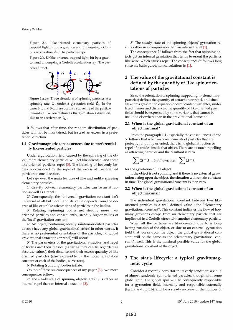
Thierry De Mees
© 2010 2 10th July 2010 - update 14th Aug
Figure 2.a. Like-oriented elementary particles of
trapped light, hit by a graviton and undergoing a Cori-
olis acceleration Ca
. The particles repel.
Figure 2.b. Unlike-oriented trapped light, hit by a gravi-
ton and undergoing a Coriolis acceleration Ca
. The par-
ticles attract.
Figure 3.a.b.c. Three situations of spinning particles at a
spinning rate ω
, under a gyrotation field Ω
. In the
cases 3.b. and 3.c. there occurs a swiveling of the particle
towards a like orientation as the gyrotation’s direction,
due to an acceleration aΩ
.
It follows that after time, the random distribution of par-
ticles will not be maintained, but instead an excess in a prefe-
rential direction.
1.4 Gravitomagnetic consequences due to preferential-ly like-oriented particles
Under a gyrotation field, caused by the spinning of the ob-
ject, more elementary particles will get like-oriented, and these
like oriented particles repel [3]. The inflating of heavenly bo-
dies is occasioned by the repel of the excess of like oriented
particles in one direction.
Let's go over the main features of like and unlike spinning
elementary particles:
1° Gravity between elementary particles can be an attrac-
tion as well as a repel.
2° Consequently, the ‘universal’ gravitation constant isn’t
universal at all but ‘local’ and its value depends from the de-
gree of like or unlike orientations of particles in the bodies.
3° Rotating (spinning) bodies get steadily more like-
oriented particles and consequently, steadily higher values of
the ‘local’ gravitation constant.
4° An object, containing ideally random-oriented particles
doesn’t have any global gravitational effect! In other words, if
there is no preferential orientation of the particles, no global
gravitational attraction (or repel) will occur!
5° The parameters of the gravitational attraction and repel
of bodies are: their masses (as far as they can be regarded as
absolute values), their distance and their excess-quantity of like
oriented particles (also expressible by the ‘local’ gravitation
constant of each of the bodies, as vectors).
6° Rotating (spinning) bodies inflate.
On top of these six consequences of my paper [3], two more
consequences follow.
7° The steady state of spinning objects’ gravity is rather an
internal repel than an internal attraction [3].
8° The steady state of the spinning objects’ gyrotation re-
sults rather in a compression than an internal repel [1].
The consequence 7° follows from the fact that spinning ob-
jects get an internal gyrotation that tends to orient the particles
like-wise, which causes repel. The consequence 8° follows long
since the basic gyrotation calculations in [1].
2 The value of the gravitational constant is defined by the quantity of like spin orien-tations of particles
Since the orientation of spinning trapped light (elementary particles) defines the quantity of attraction or repel, and since Newton’s gravitation equation doesn’t content variables, under fixed masses and distances, the quantity of like-oriented par-ticles should be expressed by some variable, that cannot be included elsewhere than in the gravitational ‘constant’.
2.1 When is the global gravitational constant of an object minimal?
From the paragraph 1.4 , especially the consequences 4° and 5° follows that when an object consists of particles that are perfectly randomly oriented, there is no global attraction or repel of particles inside that object. There are as much repelling as attracting particles and the resultant is zero.
. It follows that
for the gyrotation of the object. If the object is not spinning and if there is no external gyro-
tation acting upon the object, the situation will remain constant in time. The global gravitational constant is then zero
2.2 When is the global gravitational constant of an object maximal?
The individual gravitational constant between two like-
oriented particles is a well defined value : the “elementary
gravitational constant”. This constant indicates the flow of how
many gravitons escape from an elementary particle that are
implicated in a Coriolis effect with another elementary particle.
When all the particles are like-oriented, due to a long-
lasting rotation of the object, or due to an external gyrotation
field that works upon the object, the global gravitational con-
stant will be the same as the “elementary gravitational con-
stant” itself. This is the maximal possible value for the global
gravitational constant of the object.
3 The star’s lifecycle: a typical gravitomag-netic cycle
Consider a recently born star in its early condition: a cloud
of almost randomly spin-oriented particles, though with some
global spin. The global spin will be consequently responsible
for a gyrotation field, internally and responsible externally
(fig.1.a and fig.1.b), and for a steady increase of the number of
ω
ω
ω
Ω
Ω
Ω
aΩ
aΩ
aΩ
aΩ
0ω =∑
0Ω =∑
p190

Thierry De Mees
© 2010 3 10th July 2010 - update 14th Aug
particles with a spin orientation in the preferred direction, that
of the global star’s spin.
3.1 Towards a red giant
When an increase of like-oriented particles occurs as ex-
plained in [3], the star inflates, due to the repel of these par-
ticles. At the same time, the star’s spin velocity decreases, due
to the radius increase and to the conservation of global momen-
tum. Because the star’s density decreases, the nuclear activity
decreases at the same time. The star finally becomes a red
giant.
Now, the star’s rotation is very low and its size is maximal.
The star’s global gravitational constant became maximal as
well, because its value is directly linked to the number of like-
oriented particles [3]. But it doesn’t mean that all the particles
are like-oriented.
3.2 The spin inversion of the red giant
In my paper [2] I explained that trapped light works in two
different ways upon other trapped light: the first way is by an
orbital graviton, as explained in fig.2, the second way is the one
with a direct radial impact of ‘light’ upon other particles, as
shown in fig.4 below.
Figure 4.a. and b. Two cases of trapped light, hit by a gravi-
ton, radial or tangential, and undergoing a Coriolis effect.
From eq.(1) follows that in fig.4.a, the Coriolis effect by the
direct and radial impact of light gives an induced rotation (by a Coriolis effect), opposite of the global object’s spin. This is
particularly clear when one consider the spin iω
as one of a
more inner particle, and jω
as one of a particle that is more
situated near the star’s surface. The impact of this phenomenon, subsequently to the ex-
pansion of the star towards a red giant is that, the more the particles are like-oriented, the more the spin will tend to in-crease in the opposite direction of the star’s global spin. Indeed,
in fig.4.a, the global spin is oriented like the spins iω
and jω
.
The red giant’s spin will reach zero, then will start to in-crease in the opposite direction! Since the global gravitational constant was maximal at the end of the expansion period, this spin increase is fast, and causes the next phenomena.
3.3 Towards a white dwarf
The new spin will generate a gyrotation that is defined by
the spin of the star (fig.1.a), and that is differential, depending
from its latitude. The strongest differential spin at first will
generate a swiveling of the particles’ orientation in its neigh-
borhood, which results in an attraction with the rest of the
star’s particles, which are still oriented as before. The inner part
of the star will keep the ancient orientation the longest time
and the outer shells of the star will get inversed orientations
more quickly. This means that, still at a high value of the gravi-
tational constant, two zones are built up, which attract each-
other.
Also the global gyrotation, originated by the global spin of
the star, builds-up a compression zone between the equator
and about 35° of latitude, which compresses the star [1].
Both phenomena are responsible for a decreasing distance
between both zones, an increasing pressure and an increasing
spin of the star, strongly augmented by the law of conservation
of angular momentum when the star’s radius decreases, and
resulting all together in the collapse of the star into a white
dwarf, wherein the nuclear activity rises again strongly.
3.3 The star’s lifecycle: an harmonic?
It is quite complicated to analytically predict how the fol-
lowing stage of the white star would be, since the mixture of
‘up’ and ‘down’ oriented particles can become turbulent, and
therefore hard to evaluate. However, it is probable that due to
the global angular momentum, the dust of the dying star could
partly stay together and try another cycle, depending from
how much matter got lost into space.
4 Discussion and conclusion
A new positive test for the Coriolis Gravitation Theory: the lifecycle of a star
The expanding Sun and the lifecycles of stars have an ex-
planation that is consistent with gravitomagnetism and with
the ‘Coriolis Gravity Theory’ [2]. Rotation (spin) engenders
gyrotation, and gyrotation engenders internally more and more
like-oriented spins of elementary particles.
This results in the following lifecycle of a star: inflation of
the star occurs until it becomes a red giant at a low spin. At that
stage, its global gravitational constant is maximal. The high
number of like-oriented elementary particles also slows down
the star’s spin and inverses it, due to the Coriolis effect be-
tween like-oriented elementary particles and incoming radial
gravitons (fig.4.b).
The global gyrotation of the red giant increases together
with its inversed spin, and the places where the local gyrota-
tion is the largest will again inverse the spin of the elementary
particles. This outer shell of the star will attract the inner part
and result in a collapse to a white dwarf.
References
[ 1 ] De Mees, T., “Analytic Description of Cosmic Phenomena
Using the Heaviside Field”, Physics Essays, Vol. 18, No. 3
(2005).
[ 2 ] De Mees, T., “Is the Differential Rotation of the Sun Caused
by a Graviton Engine”, Proceedings of the NPA, (2010).
c
jω
iω
jC iC
iω
jC iC
c
c
c
jω
p191

Thierry De Mees
© 2010 4 10th July 2010 - update 14th Aug
[ 3 ] De Mees, T., “The Expanding Earth : Is the Inflation of Hea-
venly Bodies Caused by Reo-riented Particles under Gyrota-
tion Fields?”, General Science Journal, (2010).
[ 4 ] Heaviside, O., A gravitational and electromagnetic Analogy,
Part I, The Electrician, 31, 281-282 (1893)
[ 5 ] Jefimenko, O., 1991, Causality, Electromagnetic Induction,
and Gravitation, (Electret Scientific , 2000).
[ 6 ] Jefimenko, O., 2006, Gravitation and Cogravitation, (Electret
Scientific , 2006).
p192

The Expanding Earth : The Inflation of Heavenly Bo-dies Issues Demands a Compression-Free Inner Core
Explained by Gravitomagnetism
Thierry De Mees - [email protected]
Abstract
Gravitomagnetism [1] consist of Newtonian gravity and gyrotation, which is totally analogous to mag-
netism. I showed the effect of the attraction and the repulsion of spinning objects. Like-spinning objects en-
gender their mutual repel, and consequently the inflation of heavenly bodies that was suggested by the Ex-
panding Earth Theory. Here, I show that only the heavenly bodies that possess a compression-free inner core
can expand. Besides that, the Solar Protuberance Hypothesis for the formation of planets is herewith sus-
tained.
Keywords: gravitomagnetism, expanding Earth, solar protuberance hypothesis.
1. The inflation of heavenly bodies is causedby reoriented particles under gyrotationfields [2]
1.1. The expanding Earth theory
The discovery that the continental drift theory (PANGEA)
is wrong and that the Earth is instead expanding, from a small
object to the Earth of today, is about to be accepted as a stand-
ard. Also Mars is expanding and the Sun as well [2].
1.2. The internal gyrotation field of a rotating body
[1]Rotation, and the motion of bodies create fields and forces
in addition to gravity. I call this second field gyrotation, which
is the 'magnetic'-analog equivalence in gravitomagnetism and
which is responsible for the flatness of our solar system and of
our Milky Way. The gyrotation of a rotating body provides a
magnetic-like field that acts internally as well as externally to
the body upon moving masses.
Figure 1. Internal gyrotation equipotentials Ω of a spinning
body at a spinning rate ω. Surface gyrotation forces are in-
dicated as FΩ and centrifugal pseudoforces as Fc .
In figure 1 , the internal gyrotation equipotentials Ω of a
spinning body at a spinning rate ω are shown. The gyrotation
fields are parallel and oriented like the rotation vector. The sur-
face gyrotation forces are indicated as FΩ and the centrifugal
pseudoforces as FΩ . Herein Fc comes from the Lorentz force,
transposed for masses : ( )F m vΩ= ×Ω
[1].
1.3. The preferential orientation of particles under agyrotation field
In [1], it was explained that like-spinning bodies repel. This
is caused by the external gyrotation field of one spinning body
that works upon the other body. Inversely, unlike-spinning
particles attract.
Figure 2. An external gyrotation equipotential Ω of a spin-
ning body with angular velocity ω’ creates a repulsion force
upon the second spinning body.
Moreover, like spinning bodies standing above each other
have the tendency to attract and to stay
in line.
Figure 3. External gyrotation equipoten-
tials Ω of a spinning body with angular
velocity ω creates an attraction force
upon the like-spinning body that is loc-
ated beneath and above it.
© 2010 1 Thierry De Mees 17th Aug 2010 p193

Inversely, opposite spinning particles will be repulsive.
These proprieties are valid for large bodies as well as for smal-
ler particles, as shown in [2]. In order to meet this latter condi-
tion, we need to consider particles as being spinning, which is
met if we accept the concept of matter that consists of trapped
light.
2. The Earth structure with a compres-sion-free core
2.1. Two models for an Earth structure
Let us consider two possible main models of how the Earth
has been formed.
Consider in the next figure a mass (in
free space) that has been surrounded by a
thin shell of water at a certain distance. In-
deed, the water will fall upon the mass
(core). The more water falls upon the core,
the more that core will be compressed by
gravity and become very dense. The clas-
sical presentation of the Earth shows a
solid central core, an overlaying shell of
magma, and the final shell of the continents and ocean soils.
Consider now an alternative: a solid shell of mass where in
its centre, a quantity of water has been put.
The water will be attracted by the shell
and be spread over its total inside surface.
The more water is inside, the more the
shell will be compressed from the inside
by gravity. The very centre of the shell will
still preserve a net gravity of zero, and will
be attracted evenly by the shell in all direc-
tions. But the shell, supplemented with the
water, forms the gravity attraction core for
any object that is located on the outer surface of the shell. The
centre of the second model will be compression-free.
There exist evidence for none of both models. The second
model for the Earth will be studied more closely below.
2.2. Supporting considerations from the Solar Pro-
tuberance Hypothesis.The second model is not impossible at all. The Solar Pro-
tuberance Hypothesis for the formation of the planets must
provide hollow structures according the following process: a
huge electromagnetic solar protuberance (prominence) causes a
magnetic equipotential between two points A and B upon the
solar surface, in the solar corona. The hydrogen and most of the
atoms of the sun are ionized. As a result, the electrons twirl in a
very tight helix along the magnetic equipotential from point A
to point B, whereas the positive ions twirl from point B to A in
a much wider helix along that magnetic equipotential [2].
When the magnetic equipotential disappeared, the helix of pos-
itive ions attracted the electrons again and has then been pulled
apart by their mutual repulsion into large parts, that became
spinning hollow hot proto-planets. As long as the cylinder-like
proto-planets were formed of hot, spinning gasses and frag-
ments, the distribution of matter could change a bit, but as
shown in paragraph 2.1, there is no significant room for the
formation of a central solid core out of the initial hollow proto-
planet, due to the zero-gravity that is present in its centre.
When the surface of the planet’s shell of the cooled down,
as well the exterior as the interior edge of the hot gasses and
fragments, there came a moment that the outside shell got en-
tirely closed and could trap all the inside. The crust, together
with the internal magma, form the gravitation field that we
feel. The very centre of the planet has a net gravity of zero, but
all the sides of the shell (magma + crust) attract evenly any
mass in its centre. Hence, the planet’s centre is compres-
sion-free.
2.3. Supporting considerations from gravitomag-
netismIn the case of a shell-structure for the Earth, there will be a
majority of particles inside the Earth’s centre that will be ori-
ented like the Earth’s spin. This follows from the conclusions in
[5], where we discovered that the Sun’s rotation is related to
the spin orientation of its particles.
Indeed, figure 1 shows the internal gyrotation equipoten-
tials of a sphere, due to its rotation. Figure 2 shows that like-
spinning particles are repulsive and figure 3 explains the at-
traction of superimposed like-spinning particles. Consequently,
under the condition of a gravitational-free area in the centre of
the Earth, a dilatation occurs due to repulsion, perpendicularly
to the Earth spin vector. This results in a density decrease and
consequently a pressure increase in higher layers that makes
the Earth inflate.
If the Earth would have a core with a high compression, the
gyrotation dilatation forces would never overcome these com-
pression forces, and never be able to make the Earth inflate.
3. The mainstream Earth structure model
The mainstream model of the earth’s structure is ambiguousbecause it follows the first model of figure 4a, but there is onlya weak argument for the origin of the hot magma of its mantle,that is supposed to be created by the high inside compression.
3.1. The mainstream layers-model of the EarthIn figure 5 is shown where the mainstream Earth model
stands for.
Seismic waves have been send into the Earth and the reflec-
tions have been measured. Abrupt velocity changes and reflec-
tions of the waves indicate the existence of change of structure,
like solid to liquid, or soft to hard layers and vice-versa. The
Mohorovičić discontinuity (A) separates the crust and the
mantle. The Gutenberg discontinuity (B) separates the mantle
and the outer core. However, several discontinuities have been
found between the discontinuities marked as (A) and (B) in fig-
ure 5. Finally, the theoretical Lehmann discontinuity (C) separ-
ates the outer core and the inner core.
© 2010 2 Thierry De Mees 17th Aug 2010
Figure 4 a
Figure 4 b
p194

In fact, the model could only be verified for a depth of a
few thousands of kilometers, but not until the inner core,
where assumptions have been made based upon seismic meas-
urements of velocities between the transmitted and the re-
ceived waves (see next paragraph).
Figure 5. Schematic view of the interior of Earth. 1. contin-
ental crust - 2. oceanic crust - 3. upper mantle - 4. lower
mantle - 5. outer core - 6. inner core - A: Mohorovičić dis-
continuity - B: Gutenberg discontinuity - C: Lehmann dis-
continuity. The expected gravitation field strengths are
shown as well.
The mainstream gravitational field strength model inside
the Earth is based upon the densities. It increases from 9.8 m/s²
to 10.7 m/s² and then gradually decreases to zero in the Earth’s
centre.
The mainstream inside compression is as shown in the fig-
ure 6 below.
Figure 6. Mainstream compression and gravity graph [6].
These values are deduced theoretically from seismic meas-
urements (see next paragraph).
3.2. The mainstream seismic model for the Earth
Based upon the mainstream Earth model, the mainstream
interpretation of the found seismic values is given by figure 7.
Figure 7. Mainstream interpretation of the Earth’s structure
by the seismic measurements of compression waves (P-
waves) [7]. The shadow zone is occasioned by the refraction
index of the transition through the magma.
In reality, the inside Earth’s structure can only be deduced
by interpreting the transmission time of the wave between
sending and receiving (see figure 8).
Figure 8. Example of a compression velocity wave (solid
line) and a shear velocity wave (dashed line), where the
sudden velocity increase at a depth of 5155 km is inter-
preted as the evidence for a hard iron core [8].
The compression velocity wave is able to pass
through liquids (magma) but the shear velocity wave
isn’t. Remark that the velocity in the inner core is much
lower than in the mantle, which confirms a low density
of the material. A low density can be obtained by a low-
density material or by a low compression of it.
© 2010 3 Thierry De Mees 17th Aug 2010 p195

4. Discussion and conclusion: is a compressedinner core inevitable?
It is not likely that the Earth has been formed by the model
of figure 4a, due to the considerations of the chapter 2. Instead,
as well the expanding Earth as the Solar Protuberance Hypo-
thesis are favorable to a shell structure model.
On the other hand, the mainstream inner layer structure is
not harming the conditions for an expanding Earth, as far as
the inner core is compression-free. Indeed, the presence of a
hard inner core is not contradicting a compress-free zone,
while using the shell structure model for the Earth.
References
[ 1 ] De Mees, T., “Analytic Description of Cosmic Phenomena
Using the Heaviside Field”, Physics Essays, Vol. 18, No. 3
(2005).
[ 2 ] De Mees, T., “The Expanding Earth : “Is the Inflation of
Heavenly Bodies Caused by Reoriented Particles under
Gyrotation Fields?”, General Science Journal, (2010).
[ 3 ] De Mees, T., “Are Venus’ and Uranus’ tilt of natural origin?”,
General Science Journal, (2005, updated 2007).
[ 4 ] De Mees, T., “The Titius-Bode law shows a modified proto-
gas-planets' sequence”, General Science Journal, (2005, up-
dated 2006).
[ 5 ] De Mees, T., “Is the Differential Rotation of the Sun
Causedby a Coriolis Graviton Engine?”, Proceedings of the
NPA, (2010).
[ 6 ] Lawrie, W., “Fundamentals of geophysics”, (1997).
[ 7 ] http://earthquake.usgs.gov/
[ 8 ] http://knol.google.com/
© 2010 4 Thierry De Mees 17th Aug 2010 p196

© 2010 1 Thierry De Mees 7th Nov 2010
Fundamental Causes of an Attractive Gravita-tional Constant, Varying in Place and Time
Explained by Gravitomagnetism and the Coriolis Gravitation Theory
Thierry De Mees - [email protected]
Abstract
The gravitational constant G has been measured since more than 200 years [4]. It seems impossible to
find a precise value for G. In this paper, I will analyze the reasons for that issue, according Gravitomagnetism
and the Coriolis Gravitation Theory. In my paper “On the Gravitational Constant of Our Inflating Sun and
On the Origin of the Stars’ Lifecycle”, I explained that the Sun and the Earth is expanding due to Gravito-
magnetism [1] , which consist of the Newtonian gravity and gyrotation that is totally analogous to magnetism.
The Coriolis Gravitation Theory completes the picture which governs the gravitation laws. Here, the topolog-
ical values of G are found qualitatively, based on the local gyrotation field inside the Earth. I find that the dif-
ficulties for the measuring of the Gravitational Constant are caused by the location where the measurement is
done and from which location the test materials are originated. Furthermore, I come to the proof why, al-
though the Coriolis Gravity Theory allows gravitational attraction as well as repel, the heavenly bodies’ par-
ticles preferentially form distributions that are mainly attractive.
Keywords: gravitomagnetism, expanding Earth, gravitational constant, Coriolis Gravity Theory, gyrotation.
1. The Coriolis Gravitation Theory [2] [3]
1.1. Gravity between particles (trapped light) seen as a Coriolis effect
In my earlier papers [2] [3], it was explained that the gravi-
tation field can be seen as a Coriolis effect, applied upon
trapped ‘light’, where particles are made of. The relevant inte-
ractions are shown here :
Figure 1.a. Like-oriented elementary particles of trapped
‘light’, hit by an orbiting graviton and undergoing a Coriolis
acceleration Ca
. The particles repel.
Figure 1.b. Opposite-oriented trapped ‘light’, hit by an orbit-
ing graviton and undergoing a Coriolis acceleration Ca
.
The particles attract.
Attraction or repulsion are the processes that rule gravity,
caused by escaping ‘gravitons’ from opposite- or like-oriented
spins of particles. The interaction occurs, due to a Coriolis ef-
fect of the escaped graviton, interacting with the second par-
ticle’s spin. (If in the figure 1, the spin of particle ‘2’ is oriented
to the left or to the right, the acceleration will be up or down.)
1.2. The expanding Earth The repulsion variant of the Coriolis Gravitation Theory
explains the expanding of the Earth qualitatively [2]. However,
I didn’t yet treat the aspect of how the attraction and the repul-
sion can cohabit. A qualitative explanation will be given in this
paper.
2. Integration of Gravitomagnetism with the Coriolis Gravitation Theory
2.1. The early Earth and its particles’ orientation From the general point of view, one could say that the par-
ticles in the early Earth probably were oriented randomly. But the Earth was formed from a certain physical process. Al-though I am won for the idea of a solar protuberance that formed the Earth, any other process could result in some global orientation distribution of the particles.
It will be shown below that there always occurs attraction between particles, according to the figure 1.b.
2.2. Why the preferential orientation of the Earth’s par-ticles is attractive
Why is the preferential orientation of the Earth’s particles attractive? Imagine several particles side by side that are oriented upwards or downwards: ↑↓↓↑. The particles that are oriented differently, → or ← , do not affect this reasoning be-cause they don’t interact much with ↑ and ↓ (thus, the reason-ing for ↑↓↓↑ is similar to that of ↑←↓←↓→↑). As we saw earlier [2], opposite oriented particles attract and like oriented par-ticles repel. The final situation of the example is given by ↑↓ ↓↑.
2ω
1ω
1ω
2ω
p197

© 2010 2 Thierry De Mees 7th Nov 2010
Between the two downwards oriented particles of this exam-ple, the space between them increased and some room is created for another particle to fill it. We have a probability of at least 1/6 that this will be a ↑ , because ↑ is attracted by ↓ , re-sulting in a double attraction (left side and right side). In this example, we obtain a higher probability for ↑↓↑↓↑, which glo-bally is a group that is oriented upwards . The same reason-ing is possible for groups : will result in , and then in a higher distribution probability of ↓ or , which here gives a downwards super-group. These super-groups on their turn form hyper-groups the same way. However you look at it, one always gets a majority of attrac-tion-oriented compositions.
Now we know why the heavenly bodies are attractive, de-spite the fact that the Coriolis Gravity Theory allows both at-traction and repulsion of particles. We also found the first rea-son why the Gravitational Constant isn’t identical everywhere, because the super-groups’ orientations are random after all and don’t allow new settings if they became solid or crystallized.
Hereafter, we will see how the Earth’s rotation can also af-fect the Gravitational Constant value.
3. The internal gyrotation field of a rotating body [1]
3.1. Global Gyrotation fields of the Earth Rotation creates a field in addition to gravity. I called this
second field: gyrotation, which is the 'magnetic'-analog equiva-
lence in gravitomagnetism. The gyrotation of a rotating body
provides a magnetic-like field that acts internally on the indi-
vidual particles of the spinning body.
Figure 2. Internal gyrotation equipotentials Ω of a spinning
body at a spinning rate ω.
In the figure 4 , the internal gyrotation-equipotentials Ω of a
spinning body at a spinning rate ω are shown. The gyrotation
fields are parallel and oriented like the rotation vector [1].
3.2. Detailed Gyrotation fields of the Earth The actual Earth rotates at a certain rate, which creates a
gyrotation field. (This rotation probably comes from the expul-sion process out of the Sun, as I explained in my Solar Protu-berance Theory in earlier papers.)
Hereafter, I will analyze the possible outcome of the Gravi-tational Constant issue.
We found in [1] that the internal gyrotation Ω
of a sphere is given by:
( )22
int 2 3
3 2
5 3 5
r rGm Rr
c R
ωω
Ω = − − −
i
(1)
wherein R is the radius of the sphere, r the local radius of a
point inside the sphere and ω its angular velocity.
The ‘vertical’ (y-) and ‘horizontal’ (x-) components are giv-en by the following expressions, derived from (1).
( )2 2 22 3
32
5y
Gmx y R
c R
ωΩ = − + − (2)
and
2 3
3
5x
Gmxy
c R
ωΩ = (3)
These equations are visualized in the figure 3.
Figure 3.a. Vector topology of the gyrotation along the spin
axis of a spinning sphere. The spin axis contains the highest
amplitude of gyrotation. At the latitude of 35°16’, the gyro-
tation becomes zero. At the equator, gyrotation is inversed,
and one gets a local increase of the global attraction!
Figure 3.b. Rotating vector topology of the gyrotation along
the equatorial axis of a spinning sphere. At the longitude of
45°, the gyrotation is maximal. Near the center, the gyrota-
tion is zero. Since particles continuously rotate with the
Earth’s spin, their original spin orientation will not be af-
fected that easily.
p198

© 2010 3 Thierry De Mees 7th Nov 2010
The gyrotational vector topology along the spin axis shows a maximal gyrotation near the spin-axis and the center of the globe (figure 3.a). Near the latitude of 35°16’, the gyrotation becomes zero. In the equatorial direction, gyrotation is maxim-al at a latitude of 45° and zero near the center of the sphere (figure 3.b). However, since particles continuously rotate with the Earth’s spin, the gyrotational orientation is spinning as well in a plane that is parallel to the equator and their original spin orientation will not be affected that easily.
3.3. The preferential orientation of particles under a gyrotation field
The Earth’s spin is responsible of the formation of gyrota-
tion equipotential lines as shown in the figure 2. In analogy
with electromagnetism, particles will have the tendency to
orientate along the equipotentials of gyrotation. After time, the
particles will have the tendency to re-orientate along the spin
axis, parallel to it, at the amplitudes represented in figure 3.a.
The gyrotation field shown in figure 3.b will almost not affect
the particles, but a more detailed study should be done to con-
firm this.
Inversely, opposite spinning particles will be repulsive.
These proprieties are valid for large bodies as well as for small-
er particles, as shown in [2]. In order to meet this latter condi-
tion, we need to consider particles as being spinning, which is
met if we accept the concept of matter that consists of trapped
light.
4. Conclusions
In my former papers, I found that the gravitation funda-
ments are relational. That was expressed in the Coriolis Gravity
Theory.
The first important discovery in this paper is the fact that,
spites the alike occurrence of attracting and repelling particles
at the origin of the Earth, attraction became the main pattern
due to the creation of new space between the repelling par-
ticles, which is preferentially filled up by particles with an op-
posite spin. Groups of particles are randomly distributed,
which causes local changes of the Gravitational Constant. Crys-
tallized and solid matter will stop reorganize its attracting par-
ticles’ distribution. Only liquids and gasses can still continue
adapting its structure.
It follows that the values of the Gravitational Constant are
also determined by the location where the materials have been
mined from, and whereof the measuring equipment is built.
A second important discovery is that the Earth’s spin
changes bit by bit the particles’ orientation distribution in the
fluid parts of the Earth. About the Earth’s axis, the strongest
repel gyrotation field is generated, which has effects upon the
value of the internal Gravitational Constant, where the Gravita-
tional Constant increases or decreases with depth, especially in
the deeper liquid and gas zones near the poles. The increase or
decrease don’t only depend from the value of the local par-
ticles’ spin orientation, but also from the interacting orienta-
tions between large hyper-groups of different layers in the
Earth. Near the Earth’s surface, this latter interaction is pre-
ponderant.
The consequence is that the Earth expands with time in the
whole central region and along the whole spin axis. The poles
are an excellent probe region to evaluate the progress of the
value decrease of the Gravitational Constant.
At the equator, the global attraction effect between the sur-
face and the inner layers is slightly augmented, with can create
an slightly increased Gravitational Constant value between
hyper-groups over time.
Finally, I can state that it must be possible to find a way to
‘distillate’ particle spin-orientation groups that are oriented in a
particular way, in order to form an artificial attraction reduc-
tion, possibly a repel and consequently, weightlessness.
References
[ 1 ] De Mees, Thierry, “Analytic Description of Cosmic Pheno-
mena Using the Heaviside Field”, Physics Essays, Vol. 18,
No. 3 (2005).
[ 2 ] De Mees, Thierry, “The Expanding Earth : “Is the Inflation of
Heavenly Bodies Caused by Reoriented Particles under Gy-
rotation Fields?”, General Science Journal, (2010).
[ 3 ] De Mees, Thierry, “Is the Differential Rotation of the Sun
Caused by a Coriolis Graviton Engine?”, Proceedings of the
NPA, (2010).
[ 4 ] Gillies, George T., “The Newtonian gravitational constant:
recent measurements and related studies”, Rep. Prog. Phys.
60 (1997) 151–225.
p199

One day in 2002, I discovered in a newspaper that "dark matter" is supposed to be responsible for the constancy of the orbital velocity of the stars, and that velocity is supposed to be in contradiction with the Kepler laws. I was upset. We can travel to the moon and invent great medicines, we have the supposed miracle-theory of general relativity and nobody can explain it? Next hour, I was rumbling in a slide of my old desk, where I stored old papers from my university period, and I found back the analogy I made between electromagnetism and gravitation. I never trusted Einstein's relativity theory, because it only calculates what is observed by using light, but not what is really happening. Also the great Richard Feynman once confessed that he didn't understand why gravitation would be so different from other physical theories. A few days later, I found the gravitational consequences of the motion of masses. Month after month, I steadily discovered that all the cosmic issues that are not understood by mainstream, make sense through gravitomagnetism. The shape of supernovae, the disc and the spiral galaxies, the motion of asteroids, the flatness of planetary systems, the tiny rings of Saturn, black holes, the expanding Earth and Sun, etc. I can't find any cosmic issue that is in contradiction with gravitomagnetism.
Thierry De Mees
© Second edition 2011 € 32USD 39


