In proceedings of “International Conference on Computer Vision” (ICCV), Santiago, Chile, Dec. 2015 p.1

Thin Structure Estimation with Curvature Regularization

Dmitrii Marin∗, Yuchen Zhong∗, Maria Drangova∗†, Yuri Boykov∗

∗University of Western Ontario, Canada†Robarts Research Institute, Canada

dmitrii.a.marin@gmail.com yzhong.cs@gmail.com mdrangova@robarts.ca yuri@csd.uwo.ca

Abstract

Many applications in vision require estimation of thinstructures such as boundary edges, surfaces, roads, bloodvessels, neurons, etc. Unlike most previous approaches,we simultaneously detect and delineate thin structures withsub-pixel localization and real-valued orientation estima-tion. This is an ill-posed problem that requires regulariza-tion. We propose an objective function combining detectionlikelihoods with a prior minimizing curvature of the center-lines or surfaces. Unlike simple block-coordinate descent,we develop a novel algorithm that is able to perform jointoptimization of location and detection variables more ef-fectively. Our lower bound optimization algorithm appliesto quadratic or absolute curvature. The proposed early vi-sion framework is sufficiently general and it can be used inmany higher-level applications. We illustrate the advantageof our approach on a range of 2D and 3D examples.

1. IntroductionA large amount of work in computer vision is devoted to

estimation of structures like edges, center-lines, or surfacesfor fitting thin objects such as intensity boundaries, bloodvessels, neural axons, roads, or point clouds. This paperis focused on the general concept of a center-line, whichcould be defined in different ways. For example, Cannyapproach to edge detection implicitly defines a center-lineas a “ridge” of intensity gradients [6]. Standard methodsfor shape skeletons define medial axis as singularities of adistance map from a given object boundary [35, 34]. In thecontext of thin objects like edges, vessels, etc, we considera center-line to be a smooth curve minimizing orthogonalprojection errors for the points of the thin structure.

We study curvature of the center-line as a regularizationcriteria for its inference. In general, curvature is activelydiscussed in the context of thin structures. For example, itis well known that curvature of the object boundary has sig-nificant effect on the medial axis [17, 35]. In contrast, weare directly concerned with curvature of the center-line, not

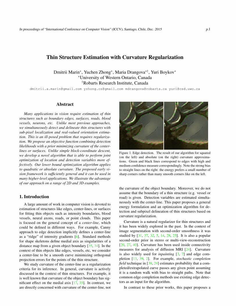
Figure 1. Edge detection. The result of our algorithm for squared(on the left) and absolute (on the right) curvature approxima-tions. Green and black lines correspond to edges with high andmedium confidence measure correspondingly. Note the strong biasto straight lines on the right: the energy prefers a small number ofsharp corners rather than many smooth corners like on the left.

the curvature of the object boundary. Moreover, we do notassume that the boundary of a thin structure (e.g. vessel orroad) is given. Detection variables are estimated simulta-neously with the center-line. This paper proposes a generalenergy formulation and an optimization algorithm for de-tection and subpixel delineation of thin structures based oncurvature regularization.

Curvature is a natural regularizer for thin structures andit has been widely explored in the past. In the context ofimage segmentation with second-order smoothness it wasstudied by [31, 37, 32, 5, 14, 28, 25]. It is also a popularsecond-order prior in stereo or multi-view-reconstruction[20, 27, 40]. Curvature has been used inside connectivitymeasures for analysis of diffusion MRI [24]. Curvatureis also widely used for inpainting [3, 7] and edge com-pletion [13, 39, 2]. For example, stochastic completionfield technique in [39, 24] estimates probability that a com-pleted/extrapolated curve passes any given point assumingit is a random walk with bias to straight paths. Note thatcommon edge completion methods use existing edge detec-tors as an input for the algorithm.

In contrast to these prior works, this paper proposes a

In proceedings of “International Conference on Computer Vision” (ICCV), Santiago, Chile, Dec. 2015 p.2

general low-level regularization framework for detectingthin structures with accurate estimation of location and ori-entation. In contrast to [39, 13, 24] we explicitly mini-mize the integral of curvature along the estimated thin struc-ture. Unlike [12] we do not use curvature for grouping pre-detected thin structures, we use curvature as a regularizerduring the detection stage.

Related work: Our regularization framework is basedon the curvature estimation formula proposed by Olsson etal. [26, 27] in the context of surface fitting to point cloudsfor multi-view reconstruction, see Fig.2(a). One assumptionin [26, 27] is that the data points are noisy readings of thesurface. While the method allows outliers, their formulationis focused on estimation of local surface patches. Our workcan be seen as a generalization to detection problems wheremajority of the data points, e.g. image pixels in Fig.2(c), arenot within a thin structure. In addition to local tangents, ourmethod estimates probability that the point is a part of thethin structure. Section 2 discusses in details this and othersignificant differences from the formulation in [26, 27].

Assuming pi and pj are neigh-boring points on a thin structure,e.g. a curve, Olsson et al. [26]evaluate local curvature as fol-lows. Let li and lj be the tangentsto the curve at points pi and pj .Then the authors propose the fol-lowing approximation for the ab-solute curvature

|κ(li, lj)| =||li − pj ||+ ||lj − pi||

||pi − pj ||

and for the squared curvature

κ2(li, lj) =||li − pj ||2 + ||lj − pi||2

||pi − pj ||2

where ||li−pj || is the distance between point pj and line li.Assume that the curve r = f(τ) is parameterized by arc-

length τ such that τ1 ≤ τ ≤ τM . If (τ1, τ2, . . . , τM ) is anincreasing parameter sequence then the curvature of f canbe approximated by∫

|κ|αdτ ≈∑

(i,j)∈N

|κ(li, lj)|α

where N = {(i, i+ 1) | i = 1, 2, . . .M − 1} is a neighbor-hood system for curve points pi = f(τi) and li = f(τi) aretheir tangent lines.

Olsson et al. [26] use regularization for fitting a surface(or curve) to a cloud of points in 3D (or 2D) space. Everyobserved point pi is treated as a noisy measurement of someunknown point pi that is the closest point on the estimatedsurface, see Fig.2(a). Each pi is associated with unknown

local surface patch li that is a tangent plane for the surface atpi. The proposed surface fitting energy combines curvature-based regularization with the first order data fidelity term

E(L) =∑

(i,j)∈N

|κ(li, lj)|αwij +∑i

1

σ2||li − pi||2 (1)

where L = {li} is the set of tangents, N is a neighbor-hood system, σ is non-negative constant, wij is a positiveconstant such that

∑j∈Ni

wij = 1. To minimize (1), thealgorithm in [26] iteratively optimizes the assignment vari-ables for a limited number of tangent proposals, and thenre-estimates tangent plane parameters, see Fig.2(a).

In contrast to [26], our method estimates thin structuresin the image grid where, a priori, it is unknown which pix-els belong to the thin structure, see Fig.2(c). We introduceset X = {xi} of indicator variables xi ∈ {0, 1} wherexi = 1 iff pixel pi belongs to the thin structure. Our ba-sic energy (2) and its extensions combine unary detectionpotentials with curvature regularization. Due to the regular-ity of our grid neighborhood, we use constant weights wij ,which are omitted from now on. We propose a different op-timization technique estimating a posteriori distribution ofxi and separate tangents li at each point. As illustrated inFig.2(b), our framework is also applicable to energy (1) andmulti-view reconstruction problem as in [26, 27].

Parent&Zucker [29] formulate a closely related trace in-ference problem for detecting curves in 2D grid. Simi-larly to us, they estimate indicator variables xi and tan-gents li. However, they estimate xi and li by enforcinga co-circularity constraint assuming given local curvatureinformation, which they estimate in advance. In contrast,we simultaneously estimate xi and li by optimizing objec-tive (2) that directly regularizes curvature of the underlyingthin structure. Moreover, [29] quantizes curvature informa-tion and tangents while our model uses real valued curvatureand tangents. The extension of [29] to 3D is not trivial.

Similarly to [26, 29] we estimate tangents only at a fi-nite set of points. Additional regularization is required ifcontinuous center-line between these points is needed [16].

Contributions: It is known that curvature of an objectboundary is an important shape descriptor [33] with a sig-nificant effect on medial axis [17, 35], which is not robusteven to minor perturbations of the boundary. In the con-text of thin objects (e.g. edges, vessels) we study a con-cept of a center-line (a smooth 1D curve minimizing thesum of projection errors), which is different from medialaxis. We regularize the curvature of the center-line. Un-like many standard methods for center-lines, we do not as-sume that the shape of the object is given and propose a gen-eral low-level vision framework for thin structure detectioncombined with sub-pixel localization and real-valued orien-tation of its center-line. Therefore, we propose an approach

In proceedings of “International Conference on Computer Vision” (ICCV), Santiago, Chile, Dec. 2015 p.3

(a) Olsson’s model [26] (b) Our model for cloud of points (c) Our model for grid pointsFigure 2. Comparison with [26]. An empty circle in (b) and (c) denotes low confidence and a dark blue circle means high confidence.

that takes into account all possible configurations of the in-dicator variables while estimating the tangents. This signif-icantly improves stability with respect to local minima. Ouroptimization method uses variational inference and trust re-gion frameworks adapted to absolute and quadratic curva-ture regularization.

Our proof-of-the-concept experiments demonstrate en-couraging results in the context of edge and vessel detectionin 2D and 3D images. In particular, we obtain promisingresults for estimating highly detailed vessels structure onhigh-resolution microscopy CT volumes. We also show ex-amples of sub-pixel edge detection regularizing curvature.While there are no databases for comparing edge detectorswith real-valued location and orientation estimation, we ob-tained competitive results on a pixel-level edge detectionbenchmark [11]. Our general early vision methodology canbe integrated into higher semantic level boundary detectiontechniques, e.g. [22], but this is outside the scope of thiswork. Our current sequential implementation is not tunedto optimize performance. Its running time for edges in 2Dimage of Fig.1 is 20 seconds and for vessels in 3D vol-ume of Fig.10 is one day. However, our method is highly-parallelizable on GPU and fast real-time performance on 2Dimages can be achieved.

In Section 2 we describe the proposed model and discussa simple block-coordinate descent optimization algorithmand its drawbacks. In Section 3 we propose a new optimiza-tion method for our energy based on variational inferenceframework. In Section 4 we describe the details of the pro-posed method and discuss the difference between squaredand absolute curvatures (Subsection 4.1). We describe sev-eral applications of the proposed framework in Section 5and conclude in Section 6.

2. Energy formulation

In the introduction we informally defined the center-lineof a thin structure as a smooth curve minimizing orthogonal

projection errors. Here we present the energy formalizingthis criterion. First we note that in our model the curve isnot defined explicitly but through points pi it passes andtangent lines li at these points. The energy is given by

E (L,X) =∑

(i,j)∈N

κ2(li, lj)xixj+

+∑i

1

σ2||li − pi||2+xi +

∑i

λixi (2)

where N is a neighborhood system, X = {xi} is a set ofindicator variables xi ∈ {0, 1} where xi = 1 iff pixel pi be-longs to the thin structure, λi define unary potentials penal-izing/rewarding presence of the structure at pi. In contrastto (1), potentials λi define the data term while 1

σ2 ||li− pi||2+is a soft constraint.

We explore two choices of the soft constraint||li − pi||+. The first one uses Euclidean distance. Inthat case it models normally distributed errors. Al-though it is appropriate for many applications, e.g.surface estimation in multi-view reconstruction [26,27], the normal errors assumption is no longer validfor the image grid because the discretization errorsare not Gaussian. In fact, using Euclidean distancemay make the soft constraint term proportional to thelength of the center-line, see illustration on the right.

d

max(0, |d| − 1)2Thus, we also propose a truncated

form of Euclidean distance:

||li− pi||+ = max(0, ||li− pi|| − 1).(3)

This does not penalize tangent lines li that are within onepixel from points pi. Different applications may require adifferent choice of no-penalty threshold.

Extensions. We can extend the energy (2) by adding otherterms that encourage various other useful properties. For

In proceedings of “International Conference on Computer Vision” (ICCV), Santiago, Chile, Dec. 2015 p.4

example, energy

E′(L,X) = E(L,X)− γ∑

(i,j)∈N

xixj (4)

for γ > 0 will reward well aligned tangents. The effect ofthis term is shown in Fig.6. This term is similar to edge “re-pulsion” in MRF-based segmentation. The overall pairwisepotential (κ(li, lj)− γ)xixj encourages edge continuity.

Another extension is to use prior knowledge about thecenter-line direction gi at pixel pi:

E′(L,X) = E(L,X) + β∑i

m(li, gi)2xi. (5)

The term m(li, gi) measures how well tangent line li isaligned with prior gi:

m(li, gi) = ||gi|| sin∠(li, gi).

The magnitude of gi constitutes the confidence measure.For example, vectors gi could be obtained from the imagegradients or the eigenvectors in the vesselness measure [9].

2.1. Block­coordinate descent optimization

To motivate our optimization approach for energy (2) de-scribed in Section 3, first we describe a simpler optimizationalgorithm and discuss its drawbacks.

The most obvious way to optimize energy (2) is a block-coordinate descent. The optimization alternates two stepsdescribed in Alg.1. The auxiliary energy optimized on line4 is a non-linear least square problem and can be optimizedby a trust-region approach, see Section 4. The auxiliaryfunction on line 5 is a non-submodular binary pairwise en-ergy that can be optimized with TRWS[18].Algorithm 1 Block-coordinate descent

1: Initialize L0 and X0

2: k ← 03: while not converged do4: Optimize Lk+1 ← argminLE(L,Xk)5: Optimize Xk+1 ← argminX E(Lk+1, X)6: k ← k + 17: end while

We found that Alg.1 is extremely sensitive to local min-ima, see Fig.3. The reason is that tangents li for points withindicator variables xki = 0 do not participate in optimiza-tion on line 4. To improve performance of block-coordinatedescent, we tried heuristics to extrapolate tangents into suchregions. We found that good heuristics should have the fol-lowing properties:

2π 2π + π

1. Since integral of curvature is sen-sitive to small local errors (see the fig-ure on the right), the extrapolating pro-cedure should yield close tangents for

Figure 3. An example of local minima for Alg.1. The more “blue”is a pixel, the more likely it is to lie on an edge. Green arrowscorrespond to pixels that were initialized as edges. Black arrowscorrespond to the edges detected by Alg.1. This local minimumconsists of two disconnected center-lines. The globally minimumsolution smoothly connects the two pieces into a single center-line.

neighbors. Otherwise step 5 of the algorithm is ineffective.This issue could be partially solved by using energy (4). Inthis case it can be beneficial to connect two tangents even ifthere is some misalignment error.

2. The heuristic should envision that some currently dis-connected curves may lie on the same center-line, see Fig.3.

The first property was easy to incorporate, while the sec-ond would require sophisticated edge continuation methods,e.g. a stochastic completion field [39, 24]. Instead we de-velop a new optimization procedure (Section 3) based onvariational inference. The advantage of our new procedureis that it is closer to joint optimization of L and X .

3. Variational InferenceIdeally, we wish to jointly optimize (2) with respect to all

variables. This is a mixed integer non-linear problem withan enormous number of variables. Thus, it is intractable.However, we can introduce elements of joint optimizationbased on stochastic variational inference framework. Theproposed approach takes into account all possible configu-rations of indicator variables xi while estimating tangentsli. This significantly improves stability w.r.t. local minima.

Energy (2) corresponds to a Gibbs distribution:

P (I,X,L′) =1

Zexp (−E(L′, X))

where Z is a normalization constant and the image is givenby data fidelity terms I = {λi}. Here I are visible vari-ables, indicator variables X and tangents L′ = {l′i} are hid-den ones. We add a prime sign for tangent notation to dis-tinguish values of random variables and parameters of thedistribution. Our goal is to approximate the posterior distri-bution P (X,L′|I) of unobserved (hidden) indicatorsX andtangents L′ given image I . The problem of approximatingthe posterior distribution has been extensively studied andis known as variational inference [4].

Variational inference is based on the decomposition

lnP (I) = L(q) + KL(q||p) (6)

where lnP (I) is the evidence, q(X,L′) is a distributionover the hidden variables, p(X,L′) = P (X,L′|I) is the

In proceedings of “International Conference on Computer Vision” (ICCV), Santiago, Chile, Dec. 2015 p.5

posterior distribution, and

L(q) =∑X

∫q(X,L′) ln

(P (I,X,L′)

q(X,L′)

)dL′, (7)

KL(q||p) = −∑X

∫q(X,L′) ln

(P (X,L′|I)q(X,L′)

)dL′.

(8)

Since KL (Kullback–Leibler divergence) is always non-negative, the functional L(q) is a lower bound for the ev-idence lnP (I). One of the nice properties of this decom-position is that the global maximum of lower bound L co-incides with the global minimum of KL(q||p) and optimalq∗(X,L′) = argmaxq L(q) is equal to the true posteriorP (X,L′|I) [4].

Unfortunately (7) cannot be optimized exactly. To makeoptimization tractable, in variational inference frameworkone assumes that q belongs to a family of suitable distri-butions. In this work we will assume that q is a factorizeddistribution (mean field theory [30]):

q(X,L′) =q(X)q(L′), (9)

q(X) =∏i

qi(xi) =∏i

qxii (1− qi)1−xi , (10)

q(L′) =∏i

δ(l′i − li) (11)

where δ(l′i − li) is a deterministic (degenerate) distributionwith parameter li. Under this assumption lower bound func-tional L becomes a function of parameters qi and li. We de-note this function L(Q,L) where Q = {qi} and L = {li}.

The proposed algorithm is defined by Alg.2. It optimizeslower bound L(Q,L) in block-coordinate fashion. The al-gorithm returns optimal tangents l∗i , see Fig.5(b), and opti-mal probabilities q∗i , see Fig.5(c).Algorithm 2 Block-Coordinate Descend for Variational In-ference

1: Initialize L0 and Q0

2: k ← 03: while not converged do4: Optimize Lk+1 ← argmaxL L(Qk, L)5: Optimize Qk+1 ← argmaxQ L(Q,Lk+1)6: k ← k + 17: end while8: return Lk, Qk

Now we consider optimization of L over L. Taking intoaccount (11), (2) and (7) we can derive

argmaxLL(Qk, L) = argmin

L

∑X

qk(X)E(X,L) =

=argminL

∑(i,j)∈N

ψijqki q

kj +

∑i

ψiqki . (12)

where

ψij ≡ κ2(li, lj),

ψi ≡1

σ2||li − pi||2+ + λi.

In case of (4) we redefine ψij ≡ κ2(li, lj) − γ, and in caseof (5) we redefine ψi ≡ 1

σ2 ||li − pi||2+ + λi + βm(li, gi).We see that optimization ofL(Qk, L) with respect toL is

a non-linear least square problem. For optimization detailsplease refer to Section 4.

The optimization w.r.t. Q can be done by coordinate de-scent. The update equation is [4]

ln q∗i (xi) = Ej =i[lnP (I,X|L)] + const =

= −xi

∑j:(i,j)∈N

ψijqj + ψi

+ const. (13)

The constant in expression (13) does not depend on xiand thus can be determined from the normalization equationqi(1)+qi(0) = 1.We initialize q0(xi) = exp(−xiψi)/(1+exp(−ψi)) on line 1 of Alg.2. We iterate over all pixels up-date step (13) on line 5 until convergence, which is guaran-teed by convexity of L with respect to each qi [4].

Note that if we further restrict q to be a degenerate dis-tribution (meaning q(xi) ∈ {0, 1}) we will get the block-coordinate descend Alg.1.

The initialization of L0 is application dependent. Inmany cases some information about direction of a thinstructure is available. Concrete initialization examples aredescribed in Section 5.

Alternative interpretations. The goal of Alg.1 is to findminL,X E(L,X), which is equivalent to

maxL

maxX

(−E(L,X)). (14)

As shown in Section 2 optimization of 14 in a block-coordinate fashion requires optimization of tangents L withfixed indicator variables X . This necessitates extrapolationof tangents. Instead we propose to optimize L taking intoaccount all possible configurations of X . That is we pro-pose to replace maximum with smooth maximum:

maxL

∑X

exp(−E(L,X)).

Then we can write down a decomposition similar to (6),which provides a lower bound yielding the same optimiza-tion procedure.

The proposed procedure is closely related to the EMalgorithm[8] where we treat tangents L as the parametersof the distribution. However, in this case the normalizationconstant of the distribution depends on L and optimizationproblem is intractable. One possible way to fix this issue isto use a pseudo likelihood [21].

In proceedings of “International Conference on Computer Vision” (ICCV), Santiago, Chile, Dec. 2015 p.6

4. Trust region for tangent estimation

Optimization of the auxiliary functions on line 4 of Al-gorithms 1 and 2 as well as energy (1) is a non-linear leastsquare problem. In [26, 27] energy (1) is optimized usingdiscrete multi-label approach in the context of surface ap-proximation. In our work we adopt the inexact Levenberg-Marquardt method in [41], which is a trust region secondorder continuous iterative optimization method.

Each iteration consists of several steps. First, the methodlinearizes:

L(qk, L+ δL) ≈ L(δL) ≡

≡∑

(i,j)∈N

(|κ(li, lj)|+

∂κ

∂liδli +

∂κ

∂ljδlj

)2

qki qkj+

+∑i

1

σ2

(||li − pi||+ +

∂d

∂liδli

)2

qki

where for compact notation we define κ ≡ |κ(li, li)| andd ≡ ||li − pi||+. We use [1] for automatic calculation ofderivatives.

Second, the algorithm solves the minimization problem

δL∗ = argminδLL(δL) + λ||δL||2

where λ is a positive damping factor, which determines thetrust region. The method uses an inexact iterative algorithmfor this task.

The last stage of iteration is to compare the predicted en-ergy change L(δL∗) − L(0) with the actual energy changeL(qk, L + δL∗) − L(0). Depending on the result of com-parison the method updates variables L and damping factorλ. For more details please refer to [41].

The most computationally expensive part of Alg.2 istrust region optimization described in this subsection. Fromthe technical point of view it consists of derivatives com-putation and basic linear algebra operations. Fortunately,these operations could be easily parallelized on GPU. Weleave the GPU implementation for a future work.

4.1. Quadratic vs Absolute Curvature

Previous sections assume squared curvature, but every-thing can be adapted to the absolute curvature too. We onlyneed to discuss how to optimize (12) for the absolute curva-ture. We use the following approximation:

||li − pj ||||pi − pj ||

≈ ||li − pj ||2

||pi − pj ||2· wij (15)

where

wij =||pi − pj ||+ ϵ

||li − pj ||+ ϵ

Figure 4. The difference between squared (left) and absolute(right) curvature approximations on an artificial example. Notethe ballooning bias of squared curvature.

and ϵ is some non-negative constant. If ϵ = 0 we have anapproximation of the absolute curvature, if ϵ→∞ we havean approximation of the squared curvature.

The trust region approach (see Section 4) works withapproximations of functions. It does not require anyparticular approximation like in the Levenberg-Marquardtmethod [19, 41]. Thus we can approximate the absolutecurvature by treating wij as constants in (15) and lineariz-ing κ(li, lj) analogously to the squared curvature case.

α

κ

sinα

α

The approximation of curvaturegiven by [26] is derived under theassumption that the angles betweenneighbor tangents are small. Under thisassumption the sine of an angle is ap-proximately equal to the angle. And theapproximation essentially computes the sines of the anglesrather than the angles themselves. As a result it significantlyunderestimates the curvature of sharp corners.

For example, let us consider the integral of absolute cur-vature over a circle and a square. The integral of the ap-proximation is 2π and 4 correspondingly, while the integralof the true absolute curvature is 2π in both cases. So the en-ergy using this approximation of absolute curvature tendsto distribute curvature into a small number of sharp cornersshowing strong bias to straight lines. Although approxima-tion of squared curvature also underestimates curvature ofsharp corners, it does not have a strong bias to straight lines.See figures 1 and 4 for comparison of the approximations.

5. Applications

5.1. Contrast edges

Here we consider an application of our method to edgedetection and real-valued edge localization.

Sobel gradient operator [36] returns the gradient magni-tude and direction for every image pixel. The high gradientmagnitude is an evidence of a contrast edge. The directionof the gradient is a probable direction of the edge. We usethe output of the gradient operator to define data fidelityterms of energy (4). For every pixel pi let gi be the gradientvector returned by the operator. We normalize vectors gi bythe sample variance of their magnitudes over the whole im-

In proceedings of “International Conference on Computer Vision” (ICCV), Santiago, Chile, Dec. 2015 p.7

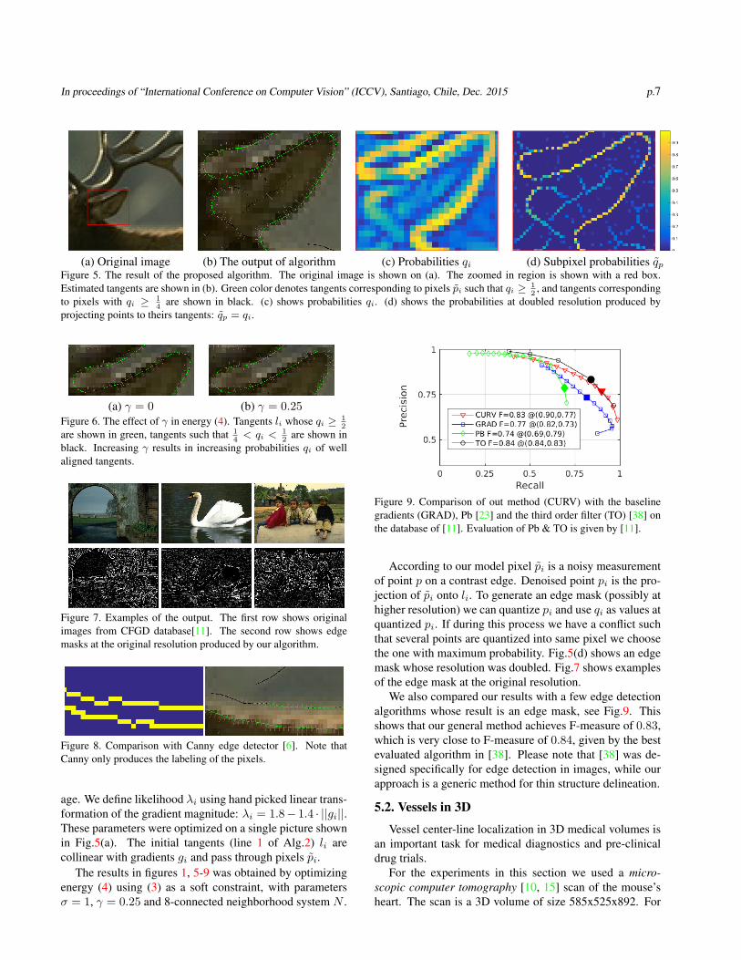
(a) Original image (b) The output of algorithm (c) Probabilities qi (d) Subpixel probabilities qpFigure 5. The result of the proposed algorithm. The original image is shown on (a). The zoomed in region is shown with a red box.Estimated tangents are shown in (b). Green color denotes tangents corresponding to pixels pi such that qi ≥ 1

2, and tangents corresponding

to pixels with qi ≥ 14

are shown in black. (c) shows probabilities qi. (d) shows the probabilities at doubled resolution produced byprojecting points to theirs tangents: qp = qi.

(a) γ = 0 (b) γ = 0.25Figure 6. The effect of γ in energy (4). Tangents li whose qi ≥ 1

2

are shown in green, tangents such that 14< qi <

12

are shown inblack. Increasing γ results in increasing probabilities qi of wellaligned tangents.

Figure 7. Examples of the output. The first row shows originalimages from CFGD database[11]. The second row shows edgemasks at the original resolution produced by our algorithm.

Figure 8. Comparison with Canny edge detector [6]. Note thatCanny only produces the labeling of the pixels.

age. We define likelihood λi using hand picked linear trans-formation of the gradient magnitude: λi = 1.8− 1.4 · ||gi||.These parameters were optimized on a single picture shownin Fig.5(a). The initial tangents (line 1 of Alg.2) li arecollinear with gradients gi and pass through pixels pi.

The results in figures 1, 5-9 was obtained by optimizingenergy (4) using (3) as a soft constraint, with parametersσ = 1, γ = 0.25 and 8-connected neighborhood system N .

Figure 9. Comparison of out method (CURV) with the baselinegradients (GRAD), Pb [23] and the third order filter (TO) [38] onthe database of [11]. Evaluation of Pb & TO is given by [11].

According to our model pixel pi is a noisy measurementof point p on a contrast edge. Denoised point pi is the pro-jection of pi onto li. To generate an edge mask (possibly athigher resolution) we can quantize pi and use qi as values atquantized pi. If during this process we have a conflict suchthat several points are quantized into same pixel we choosethe one with maximum probability. Fig.5(d) shows an edgemask whose resolution was doubled. Fig.7 shows examplesof the edge mask at the original resolution.

We also compared our results with a few edge detectionalgorithms whose result is an edge mask, see Fig.9. Thisshows that our general method achieves F-measure of 0.83,which is very close to F-measure of 0.84, given by the bestevaluated algorithm in [38]. Please note that [38] was de-signed specifically for edge detection in images, while ourapproach is a generic method for thin structure delineation.

5.2. Vessels in 3D

Vessel center-line localization in 3D medical volumes isan important task for medical diagnostics and pre-clinicaldrug trials.

For the experiments in this section we used a micro-scopic computer tomography [10, 15] scan of the mouse’sheart. The scan is a 3D volume of size 585x525x892. For

In proceedings of “International Conference on Computer Vision” (ICCV), Santiago, Chile, Dec. 2015 p.8

Figure 10. Example output of vessel center-line detection in 3D.Only tangents li with probabilities qi ≥ 1

2are shown (in purple).

Figure 11. Center-line fitting for mouse heart. Three mainbranches are show in color. Other tangents are shown in dark gray.

the both experiments the volume was preprocessed with apopular vessel detection filter of [9]. For every voxel pi thefilter returns vesselness measure vi such that higher valuesof vi indicate higher likelihood of vessel presence at pi. Thefilter also estimates direction gi and scale σi of a vessel.

For this application we use extension (5) of energy (2).

Coefficient 1σ in front of the soft constraint in the energy de-

termines how far tangents li can move from voxels p. Sincethis data has high variability in vessel thickness, we cannotuse the same σ for every voxel. We substitute σi producedby the vesselness filter for σ in energy (5):

E(L,X) =∑

(i,j)∈N

κ2(li, lj)xixj+

+∑i

(1

k2σ2i

||li − pi||2 + βm(gi, li) + λi

)xi

where k is a positive constant and λi is obtained from ves-selness measure vi by the same linear transformation thatwe use in Section 5.1. We set β = 0.5 and k = 20 and use26-connected neighborhood system N .

For the first experiment we cropped the volume forminga subvolume of size 81x187x173. We also removed 85% ofvoxels with the lowest values of vi. That yields about 3 ·106variables to be optimized. Fig.10 shows the result.

The goal of the second experiment is to extract a fewtrees describing the cardiovascular system of the wholeheart. To decrease the running time we perform Canny’s [6]hysteresis thresholding to detect one-dimensional ridges inthe volume. We substitute vesselness measure for inten-sity gradients in Canny’s procedure. Then we set qi = 1for voxels detected as ridges and qi = 0 for other voxels.This yields approximately the same number of optimizationvariables. Then we optimize tangents by the algorithm de-scribed in Section 4. Then the estimated center-line pointsare grouped based on the tangent and proximity informa-tion into a graph and a minimum spanning tree algorithmextracts the trees. The result is shown in Fig.11.

6. ConclusionWe present a novel general early-vision framework for

simultaneous detection and delineation of thin structureswith sub-pixel localization and real-valued orientation es-timation. The proposed energy combines likelihoods, indi-cator (detection) variables and squared or absolute curva-ture regularization. We present an algorithm that optimizeslocalization and orientation variables considering all pos-sible configuration of indicator variables. We discuss theproperties of the proposed energy and demonstrate a wideapplicability of the framework on 2D and 3D examples.

In the future, we plan to explore better curvature approxi-mations, extend our framework to image segmentation withcurvature regularization, and improve the running time bydeveloping parallel GPU implementation.

AcknowledgementsWe thank Olga Veksler (University of Western Ontario)

for insightful discussions.

In proceedings of “International Conference on Computer Vision” (ICCV), Santiago, Chile, Dec. 2015 p.9

References[1] S. Agarwal, K. Mierle, and Others. Ceres solver. http:

//ceres-solver.org. 6[2] T. D. Alter and R. Basri. Extracting salient curves from im-

ages: An analysis of the saliency network. IJCV, 27(1):51–69, 1998. 1

[3] L. Alvarez, P.-L. Lions, and J.-M. Morel. Image selec-tive smoothing and edge detection by nonlinear diffusion. ii.SIAM Journal on numerical analysis, 29(3):845–866, 1992.1

[4] C. M. Bishop et al. Pattern recognition and machine learn-ing, volume 4. springer New York, 2006. 4, 5

[5] K. Bredies, T. Pock, and B. Wirth. Convex relaxation of aclass of vertex penalizing functionals. Journal of Mathemat-ical Imaging and Vision, 47(3):278–302, 2013. 1

[6] J. Canny. A computational approach to edge detection.PAMI, (6):679–698, 1986. 1, 7, 8

[7] T. F. Chan and J. Shen. Nontexture inpainting by curvature-driven diffusions. Journal of Visual Communication and Im-age Representation, 12(4):436–449, 2001. 1

[8] A. P. Dempster, N. M. Laird, and D. B. Rubin. Maximumlikelihood from incomplete data via the em algorithm. Jour-nal of the royal statistical society., pages 1–38, 1977. 5

[9] A. F. Frangi, W. J. Niessen, K. L. Vincken, and M. A.Viergever. Multiscale vessel enhancement filtering. In MIC-CAI98, pages 130–137. Springer, 1998. 4, 8

[10] P. Granton, S. Pollmann, N. Ford, M. Drangova, andD. Holdsworth. Implementation of dual-and triple-energycone-beam micro-ct for postreconstruction material decom-position. Medical physics, 35(11):5030–5042, 2008. 7

[11] Y. Guo and B. Kimia. On evaluating methods for recoveringimage curve fragments. In CVPRW. 3, 7

[12] Y. Guo, N. Kumar, M. Narayanan, and B. Kimia. A multi-stage approach to curve extraction. In ECCV. 2014. 2

[13] G. Guy and G. Medioni. Inferring global perceptual contoursfrom local features. In CVPR, 1993. 1, 2

[14] S. Heber, R. Ranftl, and T. Pock. Approximate envelopeminimization for curvature regularity. In ECCV, 2012. 1

[15] D. W. Holdsworth and M. M. Thornton. Micro-ct in smallanimal and specimen imaging. Trends in Biotechnology,20(8):S34–S39, 2002. 7

[16] G. Kamberov and G. Kamberova. Ill-posed problems in sur-face and surface shape recovery. In CVPR, 2000. 2

[17] B. B. Kimia, A. R. Tannenbaum, and S. W. Zucker.Shapes, shocks, and deformations i: the components of two-dimensional shape and the reaction-diffusion space. IJCV,15(3):189–224, 1995. 1, 2

[18] V. Kolmogorov. Convergent tree-reweighted message pass-ing for energy minimization. PAMI, 28(10):1568–1583,2006. 4

[19] K. Levenberg. A method for the solution of certain non-linear problems in least squares. Quarterly of Applied Math-ematics 2, pages 164–168, 1944. 6

[20] G. Li and S. W. Zucker. Differential geometric inference insurface stereo. PAMI, 32(1):72–86, 2010. 1

[21] S. Z. Li. Markov random field modeling in image analysis.Springer Science & Business Media, 2009. 5

[22] D. Martin, C. Fowlkes, D. Tal, and J. Malik. A databaseof human segmented natural images and its application toevaluating segmentation algorithms and measuring ecologi-cal statistics. In ICCV, volume 2, pages 416–423, 2001. 3

[23] D. R. Martin, C. C. Fowlkes, and J. Malik. Learning to detectnatural image boundaries using local brightness, color, andtexture cues. PAMI, 26(5):530–549, 2004. 7

[24] P. MomayyezSiahkal and K. Siddiqi. 3d stochastic comple-tion fields for mapping connectivity in diffusion mri. PAMI,35(4):983–995, 2013. 1, 2, 4

[25] C. Nieuwenhuis, E. Toeppe, L. Gorelick, O. Veksler, andY. Boykov. Efficient squared curvature. In CVPR, Columbus,Ohio, 2014. 1

[26] C. Olsson and Y. Boykov. Curvature-based regularization forsurface approximation. In CVPR, pages 1576–1583. IEEE,2012. 2, 3, 6

[27] C. Olsson, J. Ulen, and Y. Boykov. In defense of 3d-labelstereo. In CVPR, pages 1730–1737. IEEE, 2013. 1, 2, 3, 6

[28] C. Olsson, J. Ulen, Y. Boykov, and V. Kolmogorov. Partialenumeration and curvature regularization. In ICCV, pages2936–2943. IEEE, 2013. 1

[29] P. Parent and S. W. Zucker. Trace inference, curvature con-sistency, and curve detection. PAMI, 11:823–839, 1989. 2

[30] G. Parisi. Statistical field theory, volume 4. Addison-WesleyNew York, 1988. 5

[31] T. Schoenemann, F. Kahl, and D. Cremers. Curvature reg-ularity for region-based image segmentation and inpainting:A linear programming relaxation. In ICCV, Kyoto, 2009. 1

[32] T. Schoenemann, F. Kahl, S. Masnou, and D. Cremers. Alinear framework for region-based image segmentation andinpainting involving curvature penalization. IJCV, 2012. 1

[33] T. B. Sebastian, P. N. Klein, and B. B. Kimia. Recognitionof shapes by editing their shock graphs. PAMI, 2004. 2

[34] K. Siddiqi, S. Bouix, A. Tannenbaum, and S. W. Zucker.Hamilton-jacobi skeletons. IJCV, 48(3):215–231, 2002. 1

[35] K. Siddiqi and S. Pizer. Medial representations: mathemat-ics, algorithms and applications, volume 37. Springer Sci-ence & Business Media, 2008. 1, 2

[36] I. Sobel and G. Feldman. A 3x3 isotropic gradient operatorfor image processing. 1968. 6

[37] P. Strandmark and F. Kahl. Curvature regularization forcurves and surfaces in a global optimization framework. InEMMCVPR, pages 205–218. Springer, 2011. 1

[38] A. Tamrakar and B. B. Kimia. No grouping left behind:From edges to curve fragments. In ICCV. IEEE, 2007. 7

[39] L. R. Williams and D. W. Jacobs. Stochastic completionfields: A neural model of illusory contour shape and salience.Neural Computation, 9(4):837–858, 1997. 1, 2, 4

[40] O. Woodford, P. Torr, I. Reid, and A. Fitzgibbon. Globalstereo reconstruction under second-order smoothness priors.PAMI, 31(12):2115–2128, 2009. 1

[41] S. Wright and J. N. Holt. An inexact levenberg-marquardtmethod for large sparse nonlinear least squres. The Jour-nal of the Australian Mathematical Society. Series B. AppliedMathematics, 26(04):387–403, 1985. 6