N O T I C E THIS DOCUMENT HAS BEEN REPRODUCED FROM MICROFICHE. ALTHOUGH IT IS RECOGNIZED THAT CERTAIN PORTIONS ARE ILLEGIBLE, IT IS BEING RELEASED IN THE INTEREST OF MAKING AVAILABLE AS MUCH INFORMATION AS POSSIBLE https://ntrs.nasa.gov/search.jsp?R=19810017982 2018-07-28T11:53:30+00:00Z
Transcript
N O T I C E
THIS DOCUMENT HAS BEEN REPRODUCED FROM MICROFICHE. ALTHOUGH IT IS RECOGNIZED THAT
CERTAIN PORTIONS ARE ILLEGIBLE, IT IS BEING RELEASED IN THE INTEREST OF MAKING AVAILABLE AS MUCH
OF THL EARTH'S I!cTER .IOR FROM ARTIFICIAL SATELLITES:
CONSTRAINTS ON THE REGIONAL I11PLACEMENT OF CRUSTAL RESOURCES
NAS 5-26138
John F. HermanceDepartment of Gcological Sciences
Brown UniversityProvidence, RI 02912
(881-10103) ELECTBOMM22IC DEEP- MBING(100-1000 kus) OF THE EAM I S INTERIC8 FDCBARTIFICIAL SATELLITES: CONSTRAINTS GN 282REGIONAL EBPLACEMENT GP C6USUL BESCUfiCESWuerterly Progress BeFort, 1 Oct. - 31 Dec. 63/43
N81-26519
ODclas00103
Report Due Date: December 31, 1980
t Date of Submission: January 9, 1981Period Reported October 1, 1980-December 31, 1980
RECEIVED
,.SAN 2 3 , t q?lSIS} 902.6114-001
7' Y10)5 :g:
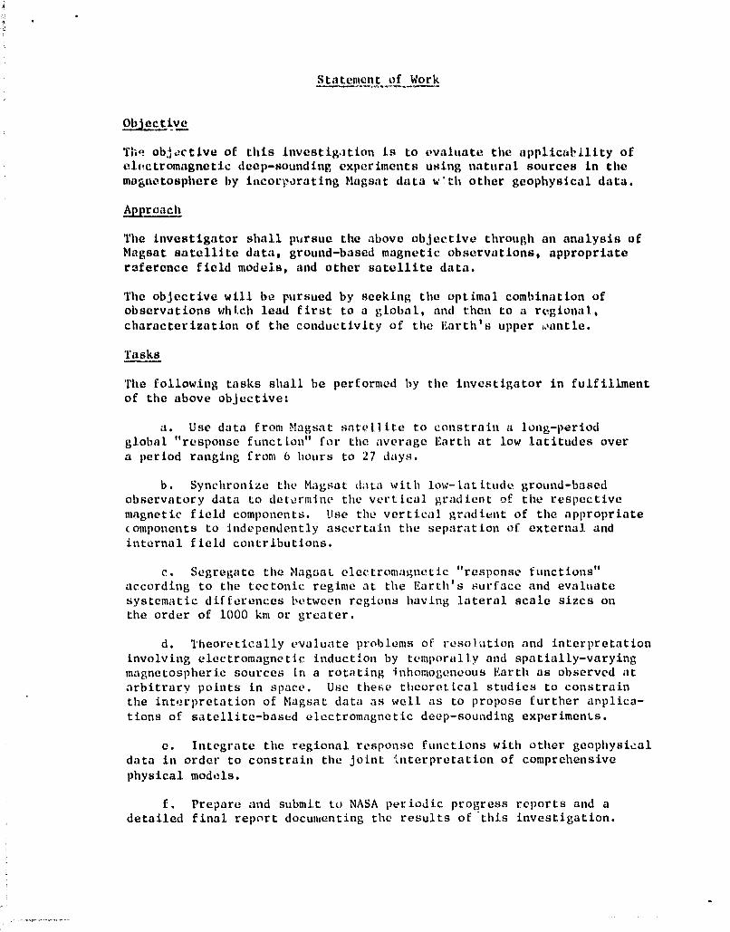
Objective
Thq objective of this investigation is to evaluate the applicability ofeleetromagnetic deep-sounding, experiments ur g ing natural sources in themagnetosphere by iacorparating Magsat data w'th other geophysical data.
Approach
The investigator shall pursue the above objective through an analysis ofMagsat satellite data, ground-based magnetic observations, appropriatereference field models, and other satellite data.
The objective will be pursued by seeking; the optimal combination ofobservations which lead first to a global, and then to a regional,characterization of the conductivity of the Earth's upper oantle.
Tasks
The following; tasks shall be performed by the investigator in fulfillmentof the above objective:
a. Use data from Magsat satellite to constrain a long-periodglobal "response function" for the average Earth at low latitudes overa period ranging from 6 hours to 27 days.
b. Synchronize the Magsat delta with low-latitude ground-basedobservatory data to determine the vertical. gradient of the respectivemagnetic field components. Use the vertical gradient of the appropriatecomponents to independently ascertain the separation of external andinternal field contributions.
c. Segregate the Maguat electromagnetic "response functions"according to the tectonic regime at the Earth's surface and evaluatesystematic differences between regions having lateral scale sizes onthe order of 1000 kin or greater.
d. 'theoretically evaluate problems of resolution and interpretationinvolving electromagnetic: induction by temporally and spatially-varyingmagnetospheric sources in a rotating; inhomog;eneous Earth as observed atarbitrary points in space. Use these theoretical studies to constrainthe interpretation of Magsat data as well as to propose further arplica-tions of satellite-based electromagnetic deep-sounding experiments.
C. Integrate the regional response functions with other geophysicaldata in order to constrain the joint interpretation of comprehensive
physical models.
f. Prepare and submit to NASA periodic progress reports and adetailed final report documenting the results of this investigation.
CONSIDERATIONS IN NOISE.-F^tEE ESTIMATES OF
GLOBAL ELECTROMAGNETIC; RESPONSE FUNCTIONS
USING SATELLITE DATA
Michael RosenGeophysical Data Analyst
John F. Hermance
Principal Investigator
Goophysical/EleeLromngnetic LaboratoryDepaAmunt of (Wologirral Sc•ivnees
Brown UnivvrsityProvidence, R. 1. 02912
December 15. 1980
1.
our preliminary goal in the MAGSAT project is to coordinate ground-based
and satellite data sets. Toward this end we have developed, and are in the final
stages of testing, a spherical harmonic analysis program which takes magnetic
data in universal time from a set of arbitrarily spaced observatories and cal-
culates a value for the instantaneous magnetic field at any point on the globe.
The calculation is done as a Last mean-squared value fit to a set of spherical
harmonics up to any desired order n.
The program is also designed to accept as a set of input parameLt.rs the
orbit position of a satellite and to coordinate it with ground-based magnetic
data for a given time. The Output is as time series for the magnetic
field on the earth's surface at the (r,O) position directly under the hypothet-,
ical orbiting satel ite foi the
duration of the LiI._3 period of the input dats
set.
Using this program to "track" the surface magnetic field beneath the sat-
ellite will allow one to compute narrow-band averaged crosspowers between the
spatially coordinated satellite and the ground-based data sets. These cross-
powers can then be used to calculate field transfer coefficients with minimum
noise distortion. As all example, we shall discuss the application of this
technique to calculating the vector response function, W.
The following variables represent a narrow-band filteted frequency
spectrum data set of the respective satellite magnetic component indicated
(we assume the NEV coordinate system):
H SAT : north component of satellite data
z SAT : vertical component of satellite data
Next, if we assume a P 0
external field, we can define:1
2.
It c - 11 SAT /Bill 0
Z c - Z SAT /Cos 0
to be the ' latitude-compensated" component.-4 of the Satellite data.
After Banks (1969), we define a vector response function W O where:
zc m wit c (2)
The usefulness of W centers oil its i tide 1jund ene e of source field details.
This result call
be cbtaimd from multi-layered spherical earth models, as
long
as the PO source field assumption is ma intal tied.
1
Noting the form (2), we introduce the term W, a
least-squares estimator
of W; if we let V stand for the statistical variance of any estimation of W,
the stintsay West frnm W, theii he fal lowing equation , J. &Iis our definition of W':
dV/dW' - did --1̂- - (<jZ c - W111 c 1 2 >)
= 0, (3)
where the angular brackets denote a frequency band average of tile form:
<(Z C_W 111 C ) (Z C_W 111 c f
(Z c (W) -10 11 C (W) ) ( ZC (W) -W 111 c M ) *d(ij
W 0 ±Awl 2
where
w0 :: center frequency of the respective filter band,
Aw: the band width of the filter,
z C (w), HC (w): elements of the respective spectra, Z c and 11 c
In general we shall term "<AB*> the "inner product" or "crossproduct"
of A and B.
3.
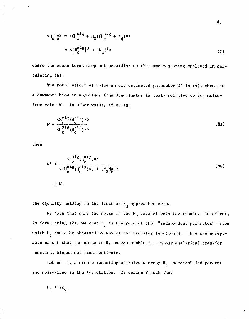
As a result of (3) we find that:
<Z 11"W
<HcH*> (4)
c c
In a noise-Free situation. W' would represent an exact calculation of W,
up to the resolution of our instruments. %s it is, however, our data will
contain noise, such that H e and Z may be expressed avi
?.c = ZS Sig + NZ
tic 11` ig + NN(5)
where NH and NZ ar4 the noise spectra associated with the ti and Z components,
respectively.
We may evaluat.: how (4) will be affected by the noise. First, we see that
the numerator, that .is, the inner product of Z and H, will be essentially unaffec-
ted. We compute:
<Z 11*> _ <(Zsif, + N. )((ii,ig)* + N*)>
Zc c c N
<Zsir,0
Sig) * i N. N* + ;igN* + N (iisif")*>Zc c it c It Z C
<Lcig(11sig)*> (6)
since <NZN*> approaches zero because of the random and uncorrelated nature of
noise sources. For the same reason, <Z Sig
N*>and <NZ (lis ig)*> approach zero asc if
well, so long, as the selectivity of the band-limiting filter applied to the
data is wide enough to allow tikes noise to average o,it.
Therefore, expression (6) supports our assertion that the numerator of
(4) is unaffected by noise. The denominator, on the other hand, is decidedly
affected:
J
,. x^i
(7)
F
<Itctl*> - < 0 cSig
+ ItN ) (11, ig + N C
<111 ,412c I+ IN II I
where the cross terms drop out according to Cie same reasoning employed in cal-
culating (6).
The total effect of noise, on
o..r estimated parameter W' in (4), then, is
a downward bias in magnitude (tile (IC110111inaLor is real) relative to its noise-
free value W. In other words, if we say
<Z *>W (8a)
<li Sig(
11c Ig) *>
c
then
W
C Cig)*} +
{N 11 N1-1)V}>(8b)
14 ,
the equality holding in
the limit as N11 approaches zero.
We note that only the noise in tile 11 C data affects the result. In effect,
in formulating (2), we cast Z C
in the role of the "independent parameter", from
which tic could be
obtained by way of the transfer function W. This Was accept-
able except that the noise in
li, unaccountable fL, in our analytical transfer
function, biased our final estimate.
Let us try a simple recasting of roles whereby 11 c "becomes" independent
and noise-free in the formulation. We define V such that
ti c M YZC 0
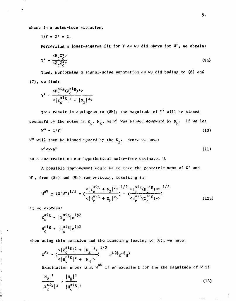
5.
where in a noise -free situation,
1/Y = Z' = Z.
Performing a least-squares fit for Y as we did above for W', we obtain:
<11 Z*:-Y1<ZGZ*>
(911)
Then, performing a signal-noise separation as we did boding to (6) and
(7), we find:
<11 Sig, zSig ) *>
<IzCig l2 + INZI2',
This result is analogous to (8b); the magnitude of Y' will be biased
downward by the noise in Z c , N Z , as W' was biased downward by N tl . If we let
W" - 1/Y' (10)
W" will then bo biaseda^.:eur b, tl:4 &: hence we have:
W' <W<w oo (11)
as a constraint on our hypothetical noise-free estimate, W.
A possible improvement would be to take the geometric mean of W' and
W", from (8b) and (9b) respectively, resulting in:
<Izsig + N I2y 1/2 "Zsig (Hsig )* , 1/2
- ( <Illc ig + NH I 2\)
( <Ns t ?, Sig )* , (12a)
If we express:
zSig Izsigl ei^
11 Sig = IH Sig leicH
then using this notation and the reasoning leading to (G), we have:
< l zsi9 I 2 + IN I2> 1/2
WAV = ( c z ) ei(^Z_^H)
< I HSig 1 2 + N t1 I >
Examination shows that W AV is an excellent for the the magnitude of W if
IN Z12 IN III,
_ - (13)1zsibl2 IHaigl2
C c
l
6.
In addition, phase information is carried noise-free in W AV , and is
shown to be, equivalent to, the difference in the phase angles of the
"hypothetienl" noise-free valt.as , "ZSigel and "Nsig". Cautioa must be
maintained, however, in using WAV for data gathered at high colatitudes,
where " Z O'4" is in general much smaller than "It ` ig". In this case the
approximate equality in (13) will break down. The necessary correction
would involve reformulating "WAV " in (l;ta) in Lite form of a weighted
geometric mean, where the weight is a function of the .appropriate coherencies.
The above discussion considered a method for extracting W from a data set
from one site (a satellite in our Instance). As we mentioned at the beginning
of this discussion, the addition or a data .set from another site, coordinated
with the primary data set, will afford us it fur more reliable method for extract-
ing noise-free parameters and, in particular, for formulra^ing W. Let us define
Mref H1e ref t)
Analogous to our definitions in (1), H ro f ropl ,e sellL:s the Latitude-corrected
narrow-band frequency spectrum for the horizontal, northern component of a
around-based data set, spatially and secularly coordinated with our satellite
components tic and lc.
Let us define a new field parameter as fellows:
<zc`iref><11 N0 >>
(lS)
c ref
where we have t:.ken (4) and replaced lid with W, We make the separation
tiref a (H Sig )sig
)* + NtiR'
and assume that there is no statistical correlation between ground-based noise
and satellite-based noise. It follows than from our arguments leading to (6)
that
F_w
<ZciA(Ii
ref )
*>
X s^H ►^ ig (Hs1g ) *^
L ref
Hence. (15) minimizeb the effects of noise in an estimate of X. However, we
must address the question of the physical interpretation of X; call be equated
with W? More specifically, what assumptions must we make about the relationship
between Ifand tic so that "X - W" maty be asserted? Another way of posing the
question would be: in a noise-free situation. what constraints must be placed
on H i*,ef so that its substitution for H* into (4) would not disturb the identity?
Mathematically, the anewcir is simple: the frequency spectrum represented
by lief
must be a scalar multiple of the frequency spectrum represented by He
for the substitution to be valid. In physical. terms, this lead: tit; to two basic
constraints; one relates to the properties of the space between the ground and
the satellite and the ether relates to the conditioning of the data ► set itself.
I For a spherically symmetric layere d eareh, assuming a pi source field,
it call shown that at or above the uppermost boundary,
BHe ' (1 + 2(r l /r) d 1U
where r is the radius of the uppermost boundary, r is the radius of the observer
(it is presumed that r > r 1 ), Ii0 is the magnitude of the external driving
field, and R is a complex response function:
(iw}jr l - 17' )
(Iwp r 1 + Z')
Z' is the surface impedance, calculated by iteration from the bottommost surface
of the model.
The space between ground and satellite must have no sharp media boundaries
and the conductivity throughout must be near-zero. Or else, reflection and/or
(l6)
(17)
attenuation of tlae field between ground sand s-satellite will occur in tin uneven
manner across the band o. the frequency spin vt.rsa of the magnetic components.
The data set conditioning must have a selectivity sufficiently narrow to
insure that the response of the earth its a whole is essentially constant over
the filter bandwidth. This last constraint r.aret,ents a tradelff with the
assumptions made to reach (6), (7), (12) and (16), our various noise-minimized
"W-estimators". We therefore must be aware of r::s spacial care necessitated in
the choice of a proper selectivity, especially with long,-period data.
We have presented these constraints under which "X W" is a good approx-
imation in a very qualitative Pannor. However, they are certainly basic problems
that must be taken into a., .:ount when applying an! , quantitative model to the data.
An attractive feraLure of the fUrmuiation proposed in (16) is the absence
of ra vertical ground-based component. This is an extremely useful property of
this analysis as it is well known that surficial lateral tnhotr.r)geneities will
introduce a distortion in the surface vertical component of far greater
magnitude than the distortion introduced in the horizontal components.
In conclusion, we make two observations. first, as W is independent of
source field details, its value as calculated from (16) should remain relatively
constant as different segment:; of the 7--odd months of MACSAT are processed via
this farmula. The size of the deviation of a set of "W's" thus calculated will
provide us with a quasi-quantitative measure of the validity of the P O source1
field assumption which underlies the vector response function's source-independent
character. This assumption can also be checked with ground-based data.
Finally, we note that although long-period data is of great use in our
analysis as it suffers least from attenuation in the atmosphere or distortion
by surficial inhomogeneities, it is also most difficult to extricate from the
9.
deta base. Satellite data close to the auroral zone must be discarded because
of the large affL-c of the field-aligned currents have on the data. Therefore,
we can have at most about 100 degrees of orbit time (about 23 minutes of data)
for a continuous data act. We ire at this time still looking for alternative
methods of chaining data sets together which minimize possible effects of