54
This presentation premiered at WaterSmart Innovations watersmartinnovations.com

This presentation premiered at WaterSmart Innovations
watersmartinnovations.com

Building Better Water Rates for an Uncertain World:Probability Management for Laypeople
Thomas W. Chesnutt, Ph.D., CAP®A & N Technical Services, Inc.http://www.antechserv.com839 Second Street, Suite 5Encinitas CA, [email protected]
David L. Mitchell M.Cubed
5358 Miles Avenue Oakland CA, 94618

The Heart of the Problem
Water rates have traditionally been focused solely on historical cost-recovery
When system costs change quickly, and perhaps unpredictably, historical rates do not reflect today’s cost consequences
Rates do not then give customers correct information to make consumptive decisions
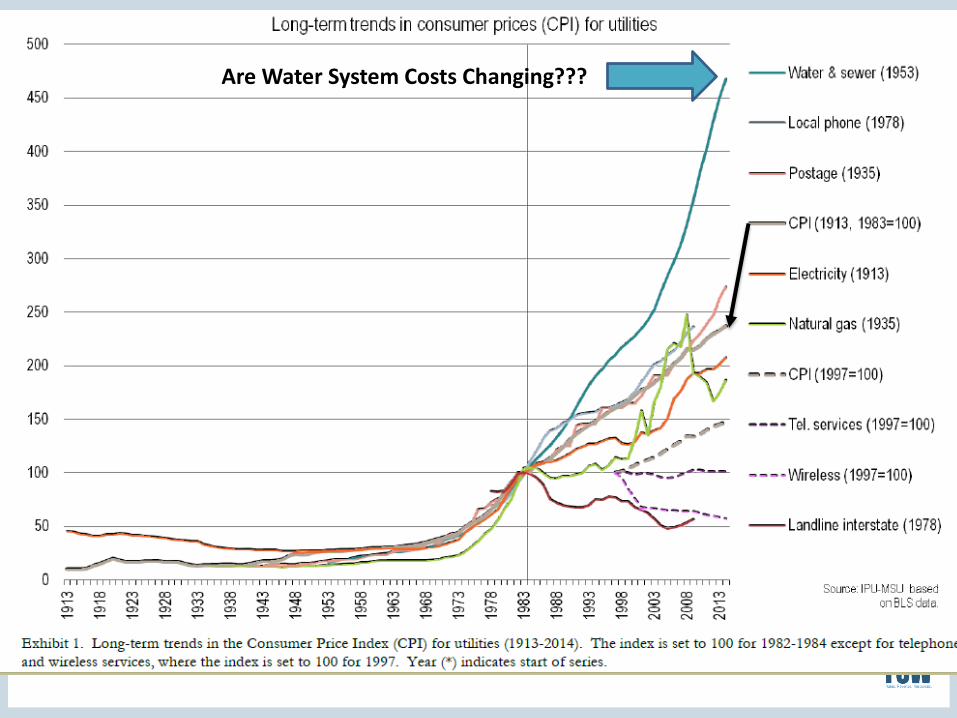
Are Water System Costs Changing???

Conservation is Part of the Solution
It is a long-term cost reducer to the utility Revenue loss is often due to other drivers Every gallon saved is water that does not have to be
pumped, treated and delivered Conservation is an investment and short-term effects
must be planned for Reduced utility costs generally mean reduced customer
rates in the long-term due to avoided infrastructure capacity increases

Financing Sustainable Water Building Better Rates in an
Uncertain World: A Handbook to explain key concepts, provide case studies and implementation advice
AWE Sales Forecasting and Rate Model: An innovative, user-friendly tool to model scenarios, solve for flaws, and incorporate uncertainty into rate making
FinancingSustainableWater.org: Web-based resources to convene the latest research and information in one location

SECTION I: IntroductionSECTION II: Today’s Imperative for Utility Financial ManagementSECTION III: The Role of RatemakingSECTION IV: Building a Better (Efficiency-Oriented) Rate StructureSECTION V: Financial Policies & Planning for Improved Fiscal HealthSECTION VI: Implementing an Efficiency-Oriented Rate Structure
Appendices Appendix A – Costing Methods Appendix B – Demand and Revenue Modeling Appendix C – AWE Sales Forecasting and Rate Model User Guide
BUILDING BETTER WATER RATESFOR AN UNCERTAIN WORLD
BALANCING REVENUE MANAGEMENT, RESOURCE EFFICIENCY, AND FISCAL SUSTAINABILITY
AWE Handbook

Flow of Economic Logic
SystemDesign
Costs
Water Rates
Demand

How Do Utilities Address This?
Ends of Water Utilities: Water Services Reliable Delivery of Quality Water Handling of Waste water, Storm water, Watershed
management By what financial means do utilities achieve
these ends? Cost Recovery (Short term) Resource Efficiency (Short and Long term) Fiscal Sustainability (Long term)

Why a New Rate Model?Typical water rate models assume that future sales are known with certainty, and do not respond to price, weather, the economy, or supply shortages—that is to say, not the world we live in.
The AWE Sales Forecasting and Rate Model addresses this deficiency: Customer Consumption Variability—weather,
drought/shortage, or external shock Demand Response—Predicting future block sales
(volume and revenue) with empirical price elasticity's
Drought Pricing—Contingency planning for revenue neutrality
Probability Management—Risk theoretic simulation of revenue risks using SIPmath®
Fiscal Sustainability—Sales forecasting over a 5 Year Time Horizon
Affordability—Can customers afford water service?
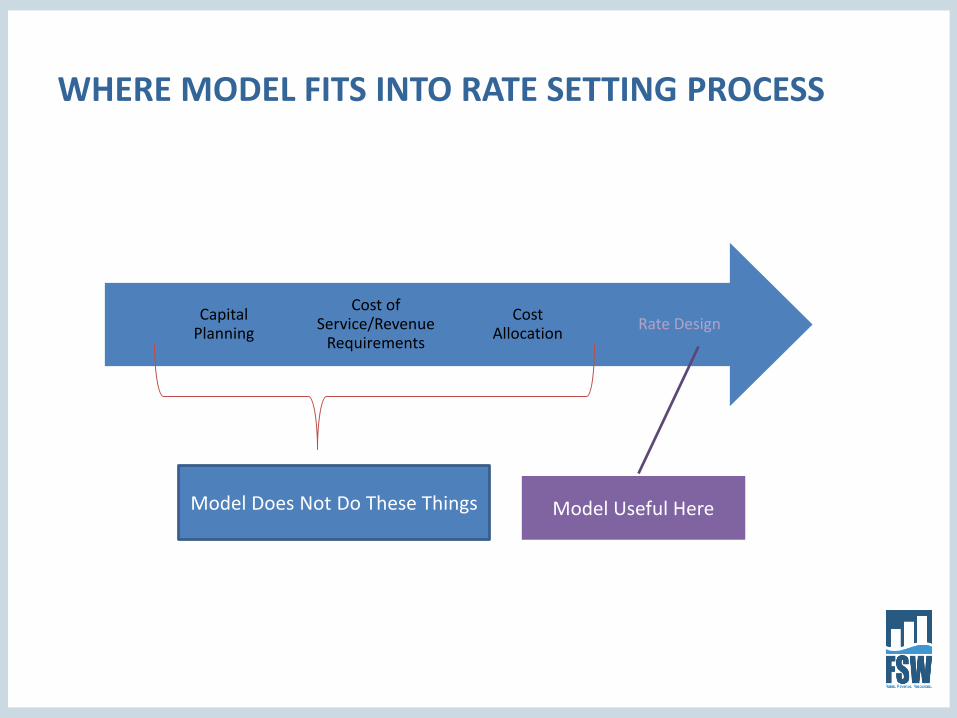
WHERE MODEL FITS INTO RATE SETTING PROCESS
Rate DesignCost Allocation
Cost of Service/Revenue
Requirements
Capital Planning
Model Useful HereModel Does Not Do These Things
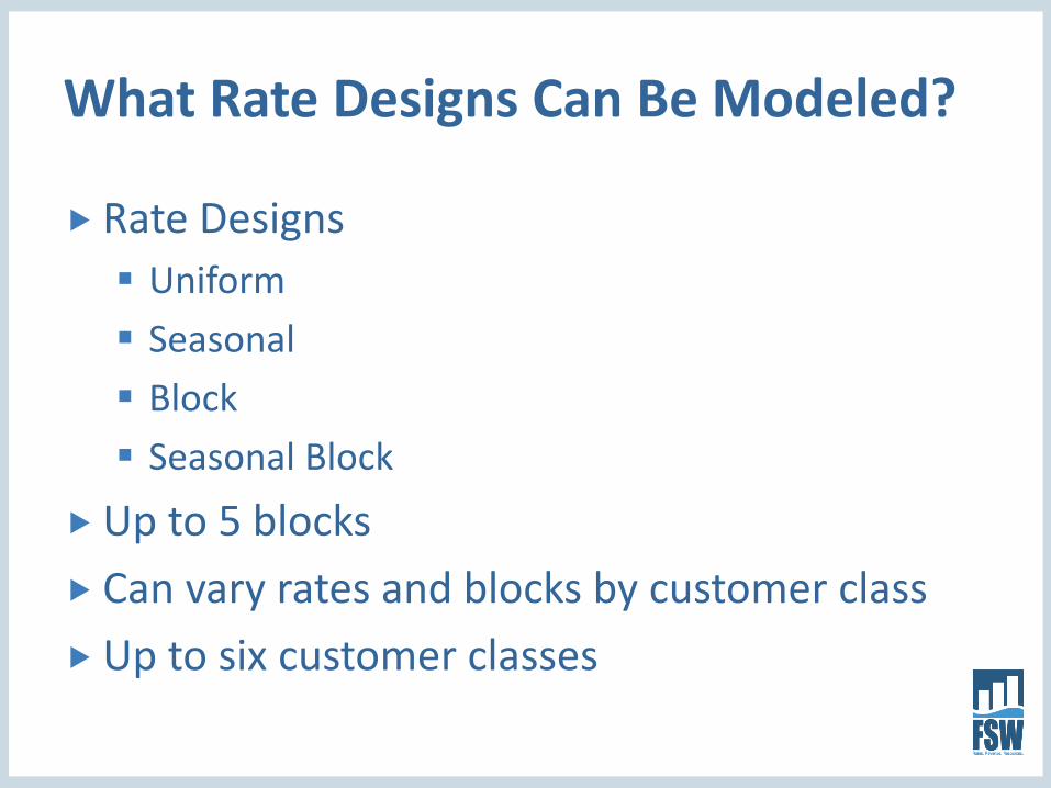
What Rate Designs Can Be Modeled?
Rate Designs Uniform Seasonal Block Seasonal Block
Up to 5 blocks Can vary rates and blocks by customer classUp to six customer classes

What Data is Needed to Use It?
Bill Tabulations from Billing System Data By Class By Season (Off-Peak, Peak)
Follows AWWA M1 Bill Tabulation Methodology
Allocating Bills to Seasons Easy when bills are rendered monthly Bit harder when bills are rendered bi-monthly or
quarterly

Bill Tabulation Screenshot

Rate Design Table
Block # Block Switch Point Rate for Block
Block 1 10 $2.50
Block 2 20 $3.00
Block 3 $3.75
Block 4 $3.75
Block 5 $3.75
Rate for first 10 units
Rate for next 10 units
Rate for units in excess of 20
Copy rate in last block to
unused blocks

Rate Design Screenshot
2. Specify rates for each Customer Class in the tables below. Save/Load Rates buttonUse the tables below to specify the Current and Proposed rates for each Customer Class. You can specify uniform, block, seasonal, and seasonal block rates.Uniform and Uniform Seasonal Designs: Enter the same rate for all five blocks. If you want the uniform rate to vary by season, set a different uniform rate for each season.Block and Seasonal Block Designs: Enter the blocks and rates for each block level. You can specify up to 5 blocks. If you want fewer blocks than 5 -- say 3 -- then enter the same rate andblock information for Block 4 and Block 5 that you did for Block 3. If you want seasonal block rates, you can specify different blocks and/or rates for each season.Mixed Designs: You can vary the rate design by Customer Class and season. For example, you can specify a block rate for the single family residential class and uniform rates for allother classes. Or you can specify a uniform rate for one season and a block rate for the other. Rate Performance by Customer Class
Single Family Off Peak Season Peak Season Annual Sales VolumeCurrent Rates Proposed Rates Current Rates Proposed Rates Current Proposed % Change
Block Rate Block Rate Block Rate Block Rate CCF 9,069,061 8,913,705 -1.7%(CCF) ($/CCF) (CCF) ($/CCF) (CCF) ($/CCF) (CCF) ($/CCF)
Block 1 5 $3.00 5 $2.50 5 $3.00 5 $3.75 Annual Revenue (Thou. $)Block 2 10 $3.00 10 $2.50 10 $3.00 10 $3.75 Current Proposed % ChangeBlock 3 15 $3.00 15 $2.50 15 $3.00 15 $3.75 Service $12,263 $12,263 0.0%Block 4 15 $3.00 15 $2.50 15 $3.00 15 $3.75 Volume $27,207 $27,744 2.0%Block 5 15 $3.00 15 $2.50 15 $3.00 15 $3.75 Total $39,470 $40,007 1.4%
AnnualSales Volume(% Change)
AnnualService & Volume Revenue
(% Change)
Impact of Proposed RatesRelative to Current Rates
0
0.2
0.4
0.6
0.8
1
1.2
-50%
-30%
-10%
10%
30%
50%
0
0.2
0.4
0.6
0.8
1
1.2
-50%
-30%
-10%
10%
30%
50%
Save/Load Rates
Rate Design Tables Rate Performance Indicators

Bill Impacts Screenshot3. Bill impacts of Proposed ratesUnder your Proposed rates, the volume charge may go up for some customers and down or stay the same for others. The Bill Impacts Table shows the percentage of bills that will godown, stay the same, or go up -- and by how much. Charts showing the distribution of bill impacts for each customer class are provided on the Bill Impacts worksheet.
Affordability Index% Change in Average and Median Annual Water Service Cost by Customer Class Current ProposedAverage Annual Water Service Cost Median Annual Water Service Cost Affordability index equals
Customer Class Current Proposed % Change Current Proposed % Change the median annual waterSingle Family $777 $804 3.4% $650 $672 3.3% cost for the primaryMulti Family $4,254 $4,294 0.9% $1,930 $1,942 0.6% residential customer classCII $3,323 $3,382 1.8% $1,481 $1,504 1.5% divided by medianLandscape $5,599 $6,007 7.3% $2,503 $2,720 8.7% household income.Not in useNot in use
Bill Impacts Table% of bills decreasing by No More Than % of bills increasing by
Customer Class more than 20% 15 to 20% 10 to 15% 5 to 10% +/- 5% 5 to 10% 10 to 15% 15 to 20% more than 20%Single Family 0% 0% 21% 38% 9% 4% 17% 11% 0%Multi Family 0% 1% 38% 25% 4% 4% 18% 12% 0%CII 0% 0% 25% 20% 28% 7% 9% 10% 0%Landscape 0% 0% 26% 12% 33% 2% 6% 20% 0%Not in useNot in use
0.0%
1.0%
2.0%
3.0%
4.0%
5.0%
0.0%
1.0%
2.0%
3.0%
4.0%
5.0%
0%
10%
20%
30%
40%
50%
more than 20% 15 to 20% 10 to 15% 5 to 10% 5 to 10% 10 to 15% 15 to 20% more than 20%
Per
cen
t o
f B
ills
Single Family Customer Class Bill Impact Histogram
% Decrease in Bill % Increase in Bill
No More Than+/- 5%
Avg and median bill
impacts
Bill Impact Histograms
Affordability Indicator
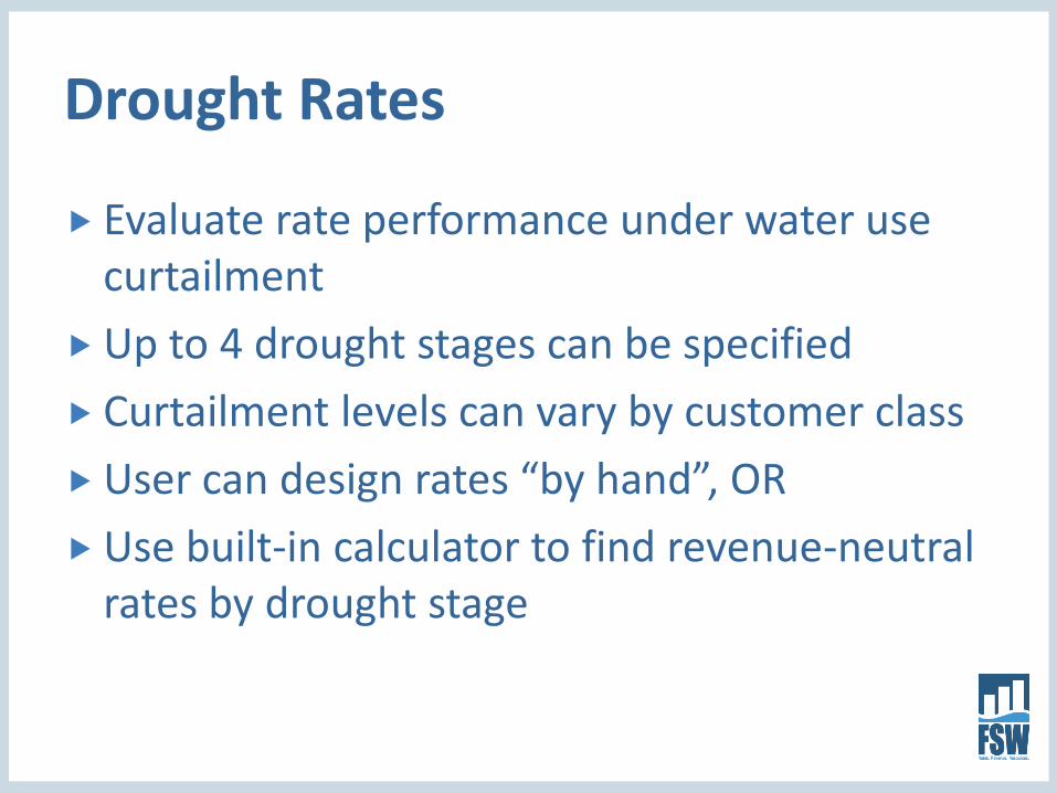
Drought Rates
Evaluate rate performance under water use curtailment
Up to 4 drought stages can be specified Curtailment levels can vary by customer classUser can design rates “by hand”, ORUse built-in calculator to find revenue-neutral
rates by drought stage
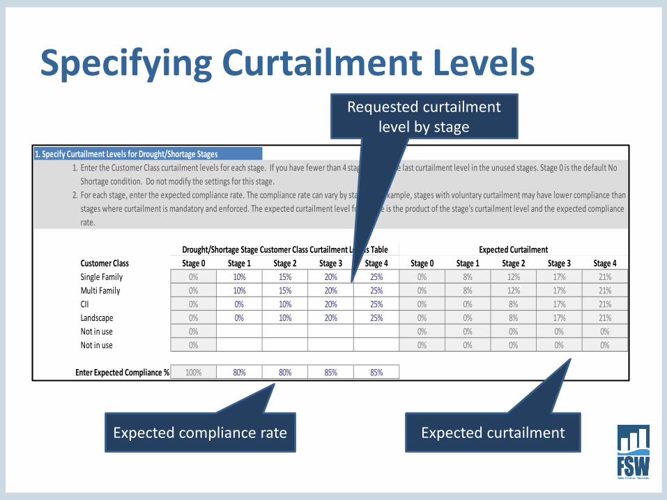
Specifying Curtailment Levels
1. Specify Curtailment Levels for Drought/Shortage Stages1. Enter the Customer Class curtailment levels for each stage. If you have fewer than 4 stages, enter the last curtailment level in the unused stages. Stage 0 is the default No
Shortage condition. Do not modify the settings for this stage.2. For each stage, enter the expected compliance rate. The compliance rate can vary by stage. For example, stages with voluntary curtailment may have lower compliance than
stages where curtailment is mandatory and enforced. The expected curtailment level for a stage is the product of the stage's curtailment level and the expected compliancerate.
Drought/Shortage Stage Customer Class Curtailment Levels Table Expected CurtailmentCustomer Class Stage 0 Stage 1 Stage 2 Stage 3 Stage 4 Stage 0 Stage 1 Stage 2 Stage 3 Stage 4Single Family 0% 10% 15% 20% 25% 0% 8% 12% 17% 21%Multi Family 0% 10% 15% 20% 25% 0% 8% 12% 17% 21%CII 0% 0% 10% 20% 25% 0% 0% 8% 17% 21%Landscape 0% 0% 10% 20% 25% 0% 0% 8% 17% 21%Not in use 0% 0% 0% 0% 0% 0%Not in use 0% 0% 0% 0% 0% 0%
Enter Expected Compliance % 100% 80% 80% 85% 85%
Requested curtailment level by stage
Expected compliance rate Expected curtailment

Designing Drought Rates
2. Rate Performance by Drought/Shortage StageThe tables in this section hold two sets of rates. Your proposed rates are carried over from Step 3. These cannot be modified on this worksheet. They provide the point of referencefor calculating the revenue impacts of drought stages. The Stage rates are the rates that would apply for a given drought/shortage stage. To see how your Proposed rates would perform ina drought stage, click the Reset Drought Stage Rates to Proposed Rates. This will copy your Proposed rates into the tables for the Stage Rates. You can then use the Select Drought Stagedrop-down list to cycle through the drought stages and see how your sales revenue would be impacted by each stage. Impacts to annual sales volume and revenue for each Customer Class Select Drought Stageare summarized to the right of the rate tables. You can adjust the Stage Rates to see how your annual sales volume and revenue would respond. You can adjust the size or number of blocksas well as the rates for each block. You can use trial and error to find rates appropriate to each drought/shortage stage, or you can use Excel's goal-seek or solver functionality to do this. Section 3 provides a calculator that can quickly identify rates for a given drought/shortage stage that are revenue neutral. Rate Performance by Customer Class
Single Family Off Peak Season Peak Season Annual Sales VolumeProposed Rates Stage 2 Rates Proposed Rates Stage 2 Rates Proposed Stage 2 % Change
Block Rate Block Rate Block Rate Block Rate CCF 8,913,705 7,844,060 -12.0%(CCF) ($/CCF) (CCF) ($/CCF) (CCF) ($/CCF) (CCF) ($/CCF)
Block 1 5 $2.50 5 $2.50 5 $3.75 5 $3.75 Annual Sales Revenue (Thou. $)Block 2 10 $2.50 10 $2.50 10 $3.75 10 $3.75 Proposed Stage 2 % ChangeBlock 3 15 $2.50 15 $2.50 15 $3.75 15 $3.75 Service $12,263 $12,263 0.0%Block 4 15 $2.50 15 $2.50 15 $3.75 15 $3.75 Volume $27,744 $24,415 -12.0%Block 5 15 $2.50 15 $2.50 15 $3.75 15 $3.75 Total $40,007 $36,678 -8.3%
AnnualSales Volume(% Change)
AnnualService & Volume Revenue
(% Change)
Impact of Drought Stage Rates Relative to Proposed Rates
0
0.2
0.4
0.6
0.8
1
1.2
-50%
-30%
-10%
10%
30%
50%
0
0.2
0.4
0.6
0.8
1
1.2
-50%
-30%
-10%
10%
30%
50%
Rate Design TablesRate Performance
Indicators
Drought Stage Selector

Drought Rate Calculator3. Calculate Revenue Neutral Rates by Drought StageThe revenue neutral rates calculator will quickly find a set of rates for a given drought/shortage stage that will generate the same revenue as your Proposed rates under a no shortagecondition. There are four steps to using the calculator:
1. Choose the drought/shortage stage you want to calculate rates for.2. Choose the method for calculating the rates. There are two choices. The first choice is to adjust your Proposed rates so that each customer class generates the same revenue
it would have generated under your Proposed rates assuming no use curtailment. This may result in significant differences across classes in the amount by which rates areadjusted. The second choice is to adjust your Proposed rates so that all classes when grouped together are revenue neutral. Rates across classes will be adjusted by the sameproportionate amount. Revenue neutrality may not hold for individual classes, but overall revenue will be neutral to the Proposed rates assuming no use curtailment.
3. Complete the Leave or Adjust Rate in Block table below. Choose Leave if you want the rate in the block to be the same as it is for your Proposed rates. Choose Adjust if youwant the calculator to adjust this rate. For example, if you only want to adjust the upper block rates, choose Leave for lower blocks and Adjust for upper blocks. If you havefewer than 5 blocks, set the unused blocks to the same setting used for your last block.
4. Make desired adjustments to the block widths for the Stage Rates in the Stage Rates tables above.5. Click the Find Revenue Neutral Rates button.
Note: The calculator will overwrite the rates that are in the Stage Rates tables above. If you want to preserve these rates, save them as a rate scenario by clicking the Save/Load Ratesbutton before using the calculator.
Choose Drought Stage to Evaluate:
Choose Method for Calculating Revenue Neutral Rates:
Leave or Adjust Rate in Block?
Class Block 1 Block 2 Block 3 Block 4 Block 5Single Family Leave Adjust Adjust Adjust AdjustMulti Family Leave Adjust Adjust Adjust AdjustCII Leave Adjust Adjust Adjust AdjustLandscape Leave Adjust Adjust Adjust AdjustNot in use Leave Leave Leave Leave LeaveNot in use Leave Leave Leave Leave Leave
Find Revenue Neutral Rates
Reset Drought Stage Rates to Proposed Rates
Save/Load Rates

Limitations of the Rate Design Module
Results only as good as the bill tabulationdata
Can only evaluate how rates will perform ON AVERAGE
Does not provide insight into VARIABILITY of performance
That’s where the Revenue Simulation Modulesteps in
Plans based on average assumptions are wrong on average --Sam Savage, The Flaw of Averages

Revenue Simulation Module

Questions the Simulation Module Can Address
What is the likelihood we will meet our one-year, three-year, five-year revenue targets under our current or proposed rates?
What is the chance our revenues will turn out more than 15% below our current projections?
What level of confidence can we have that our sales will exceed our minimum planning estimates?

What is Net Revenue Volatility? Empirical view of Volatility: Definition in Finance
One year change
Big Scary Question: How does sales variation affect Net Revenues(Revenues minus Costs)
Typically the more revenues collected on variable/commodity charges the more potential for revenue volatility (up and down) Exception: Seasonal Rates (Peak season demand can be less variable)

Annual Sales Volatility, standard deviation of ≈ 7 %
Net Revenue = Revenue – Costs±2.6%
Short Term Uncertainty looks
manageable;Don’t Celebrate Yet.
Monte Carlo Simulation
Results
-
=
Short Term: The Shape of Uncertainty and Revenue Risk

ProbabilityManagement.org
Sam Savage onCuring the Flaw of Averages

Average Outcome vs. Likely OutcomesFlaw of Averages Fact 1 – Planning for the future is rife with
uncertainties.Fact 2 - Most people are not happy with Fact 1 and
prefer to think of the future in terms of average outcomes.
Fact 3 - The “flaw of averages” states that plans based on average assumptions are, on average, wrong. -adapted from Savage (2012) Flaw of Averages
www.probabilitymanagment.org
The cyclist is safe on the average path On average, the
cyclist is dead.

Do Water Sales stay on the average path?Then why do water sales forecasts?
Answer: They don’t have to.AWE Sales Forecasting and Rate Model: Open Source Drought Rateshttp://www.financingsustainablewater.org/tools/awe-sales-forecasting-and-rate-model

Towards an Alternative Decision-Making Framework
Information can reduce uncertainty. Information that cannot effect a decision has no strategic value.
Interactive simulation is a strategy for explicitly displaying the effects of a decision on uncertain outcomes.
Diversification—spreading risk over a variety of outcomes—helps minimize the likelihood of extreme outcomes.
SIPs and SLURPs of Water Interactive simulation and visualization better
communicate decision uncertainties SIP – Stochastic Information Packets
• In the SIPmath™ 2.0 Standard, uncertainties are communicated as data arrays called SIPs (Stochastic Information Packets). Thus random draws from uncertain possibilities are stored as a column of realizations.
SLURP – Stochastic Library Unit Relations Preserved• A coherent set of SIPs that preserve statistical
relationships between uncertainties is known as a Stochastic Library Unit with Relationships Preserved (SLURP).

Stochastic Information Packets (SIPs)• SIPs advance the modeling of uncertainty.
• SIPs are:• Actionable• Additive• Auditable

SIPMath™ is ActionableSips can be used directly in calculations of uncertainty.Cells in Excel can refer to SIPs instead of a single number.No macros or add-ins need remain in the spreadsheet.
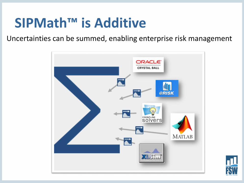
SIPMath™ is AdditiveUncertainties can be summed, enabling enterprise risk management

SIPMath™ is Auditable
The SIPMath™ standard requires provenance. Saved SIPs can be replicated using same seed=auditability.

How Does Probability Management Work in The AWE Rate Model? The model focuses on three variables that are key
to short-run revenue performance: Weather (historical or synthetic) Growth (projected) Supply disruption/use curtailment (correlated to
weather) Two rate designs are simultaneously evaluated: Current rate (reference condition) Proposed rate
Simulation enacted with SIPmath®

Simulation Process
2. Calculate model
3. Save result(trial)
1. Draw model variables from
their probability distributions
A cycle constitutes 1 trial. In the Revenue Simulation Module, User can simulate 10, 100, 500, or 1000 trials.

Why Simulate?
Alternatives to simulation are: Ignore uncertainty (a common strategy) Construct scenarios (also common) Both are problematic
Simulation offers: More complete enumeration of possible
outcomes Likelihood of particular outcomes

Simulation of Sales Revenue Distribution

Additional Data Needed for Module
Weather Monthly Precipitation and Temperature data for
Service Area• Historical (up to 90 years), OR• Synthetic (for example, to simulate impact of climate change)
Easy to get historical weather data for service areas –Guidebook recommends several sources for weather data
Customer Class Account Growth User specifies Low, Medium, High Account Growth
Rates, by Class

Weather Data Screenshot: Two SIPs make a SLURP
Step 6: Enter Weather Data to be Used by Revenue Simulation ModuleOn this worksheet you enter historical monthly precipitation and temperature data for your service area. The model will use this data to simulate how your demands may vary in response to deviations from normal weather patterns.You can enter up to a maximum of 90 years of historical data -- 1924-2013. Your historical data must be contiguous -- there cannot be gaps between years. It also must be complete across months. The model will ignore years where these conditions are not met.It is not required that you provide data for all 90 years. For example, if you only have data for the period 1982-2012 you can enter that in the approprate rows of the tables. To get reliable results, however, it is strongly recommended you enter at least 15 years of data.Consult the user guide for information on weather data sources.Go back to Revenue Simulation Module Worksheet Go forward to Step 7: Setup Simulation Worksheet
1. Set most recent year in your weather dataEnter the most recent year for which you are providing weather data.
Most recent year: 2012
2. Enter Monthly Precipitation Totals (in) 3. Enter Monthly Average Maximum Air Temperature (degrees F)Enter total monthly precipitation in inches for each year of weather data you have for your service area. Enter the monthly average daily maximum air temperature in degrees Fahrenheit for each year of weather data you have for your
service area. Be sure you are entering average daily maximum air temperature and not average daily air temperature.
Year Jan Feb Mar Apr May Jun Jul Aug Sep Oct Nov Dec Year Jan Feb Mar Apr May Jun Jul Aug Sep Oct Nov Dec2012 2.91 1.18 4.17 2.56 0.00 0.04 0.00 0.00 0.00 0.87 4.09 5.83 2012 61.0 63.0 63.0 70.6 78.6 82.9 85.9 87.3 83.4 75.7 65.8 56.92011 1.18 4.06 6.26 0.28 0.79 1.93 0.00 0.00 0.00 0.91 1.22 0.08 2011 56.2 60.5 62.7 69.0 72.4 79.2 84.3 84.5 86.4 76.5 62.8 60.02010 5.71 2.80 1.93 3.82 1.06 0.00 0.00 0.00 0.00 0.83 1.85 5.71 2010 55.1 60.8 65.3 66.1 72.5 82.6 84.1 83.3 85.2 74.9 64.7 57.22009 1.02 6.34 2.36 1.22 0.71 0.00 0.00 0.00 0.16 3.74 0.59 2.40 2009 60.4 59.1 65.4 70.6 78.6 80.4 86.6 87.1 88.0 73.3 65.7 54.62008 7.13 1.85 0.12 0.08 0.00 0.00 0.00 0.00 0.00 0.04 2.36 1.81 2008 53.7 60.8 66.5 71.6 77.7 85.3 86.7 88.5 85.1 78.1 66.9 54.72007 0.43 3.70 0.24 0.59 0.28 0.00 0.00 0.00 0.12 1.22 0.75 2.40 2007 58.2 60.8 70.5 72.2 77.7 83.9 86.1 87.0 80.8 72.9 67.4 55.92006 2.24 1.97 6.26 4.25 1.02 0.00 0.00 0.00 0.00 0.12 1.42 2.95 2006 58.5 63.2 59.3 66.0 77.8 84.9 91.8 83.9 83.0 74.0 64.2 57.92005 4.33 3.31 2.60 1.46 1.26 0.28 0.00 0.00 0.00 0.12 0.94 10.04 2005 52.7 61.3 67.0 68.8 74.9 78.7 89.7 87.2 80.1 75.6 67.8 58.82004 2.48 5.04 0.91 0.08 0.08 0.00 0.00 0.00 0.08 2.64 2.17 3.90 2004 55.1 59.7 74.0 75.0 77.9 83.2 85.9 87.0 86.7 73.1 62.2 56.82003 1.14 0.98 1.46 3.58 0.51 0.00 0.00 0.00 0.00 0.00 1.65 5.94 2003 59.2 61.5 67.6 64.9 76.6 83.3 91.1 86.3 86.6 81.5 61.7 56.62002 0.75 1.54 1.89 0.16 1.18 0.00 0.00 0.00 0.00 0.00 2.40 8.66 2002 55.0 63.0 64.6 69.5 76.1 84.0 87.5 86.1 86.1 76.2 66.9 58.12001 1.89 5.51 1.10 1.14 0.00 0.12 0.00 0.00 0.12 0.28 3.58 7.01 2001 57.0 59.2 69.1 67.9 85.9 87.2 84.0 86.4 82.1 78.7 65.9 55.72000 5.79 8.11 2.01 0.79 1.14 0.08 0.00 0.00 0.04 1.34 0.75 0.39 2000 58.8 60.0 66.5 72.9 76.9 84.5 82.5 86.1 84.3 73.1 61.0 59.31999 2.76 5.12 2.48 1.69 0.08 0.00 0.00 0.00 0.00 0.31 2.05 0.51 1999 55.3 58.5 60.8 69.1 73.0 80.7 83.2 83.3 82.8 79.3 66.4 61.21998 8.03 12.20 2.09 1.26 2.64 0.00 0.00 0.00 0.16 0.79 3.07 0.67 1998 56.3 57.6 64.9 67.5 67.3 76.5 85.4 88.9 82.6 73.8 62.3 55.31997 8.19 0.20 0.24 0.24 0.28 0.20 0.00 0.47 0.00 0.79 5.47 2.56 1997 56.0 63.4 69.9 73.1 82.6 83.0 86.5 84.6 86.1 75.2 65.5 56.51996 5.28 5.94 2.44 1.81 1.77 0.00 0.00 0.00 0.00 0.91 2.72 6.89 1996 57.9 62.1 67.1 72.9 77.5 84.3 89.5 88.9 82.1 75.5 65.1 59.01995 9.84 0.20 8.62 1.06 1.22 1.18 0.00 0.00 0.00 0.00 0.00 6.77 1995 57.1 61.3 62.2 68.3 71.7 79.9 86.2 87.7 83.8 79.2 71.2 59.91994 1.77 3.94 0.20 0.87 1.61 0.00 0.00 0.00 0.00 0.67 5.91 2.48 1994 58.2 58.4 68.4 70.9 74.1 83.4 84.4 87.0 82.4 75.3 58.0 53.01993 8.46 4.25 2.13 0.59 0.55 0.39 0.00 0.00 0.00 0.31 2.52 2.36 1993 54.8 58.7 67.2 69.9 75.8 84.6 85.7 86.6 84.1 76.8 65.3 55.01992 1.38 5.94 3.11 0.31 0.00 0.28 0.00 0.00 0.00 1.38 0.16 6.02 1992 52.8 63.7 65.7 74.8 81.9 80.8 85.7 88.8 84.9 79.1 66.6 54.2
Can enter up to 90 yrs. Need at least 15. More is better than less.
Can modify historical weather for future climate change if desired.

Calculation of Weather Effects Based on CUWCC GPCD Weather Normalization
Methodology and Empirical Model Accounts for Seasonal Shape of Demand Relative Importance of (weather sensitive) Outdoor Use
Monthly effects formed into weighted-average seasonal effect
Weighting accounts for: Monthly contribution to total seasonal use Strength of monthly weather effect on total seasonal use
Weather effect coefficients can be modified by user

Uncertain Account Growth
Can simulate with or without growth uncertainty No Growth Certain Growth Uncertain Growth
If Uncertain Growth, then Low, Medium, High Growth Rates transformed into probability distribution Normal Triangular Uniform
User specifies which distribution to use

Water Use Curtailments
Three Choices Exclude from simulation Associate with historical weather (preferred
method) Specify likelihood

Are Future Sales and Revenue Uncertain?

Drought Pricing Shortages are when, not if. Imposing curtailments on
customers affects revenues This can be planned for,
communicated, and effectively implemented.

Drought Let’s talk probability and evidence What is the probability of a more than one decade-long
drought? …Where? When? In the Southwest US Within a 50 year period,
• 1950 to 2000?• Or better 2050-2099?
Odds and “P” Value1 in 100 ≡ P011 in 10 ≡ 10 in 100 ≡ P101 in 5 ≡ 20 in 100 ≡ P20
50

Answer - P80 [I’m not making this up.]
advances.sciencemag.org/content/advances/1/1/e1400082.full.pdf
This will be on the test…new vocabulary
• Megadrought• Semi-permanent drought
51

Associate Drought Stage with Historical Weather
3. Enter Monthly Average Maximum Air Temperature (degrees F) 4. Enter Drought Shortage StageEnter the monthly average daily maximum air temperature in degrees Fahrenheit for each year of weather data you have for your (Optional) For each hydrologic year you can select what drought/shortage stage service area. Be sure you are entering average daily maximum air temperature and not average daily air temperature. would have applied given your current system supplies and customer demands.
You can then have the model use this information when it simulates water sales.This is explained further in Step 5 Setup Simulation.
Year Jan Feb Mar Apr May Jun Jul Aug Sep Oct Nov Dec Stage Index2012 61.0 63.0 63.0 70.6 78.6 82.9 85.9 87.3 83.4 75.7 65.8 56.9 Stage 0 02011 56.2 60.5 62.7 69.0 72.4 79.2 84.3 84.5 86.4 76.5 62.8 60.0 Stage 0 02010 55.1 60.8 65.3 66.1 72.5 82.6 84.1 83.3 85.2 74.9 64.7 57.2 Stage 0 02009 60.4 59.1 65.4 70.6 78.6 80.4 86.6 87.1 88.0 73.3 65.7 54.6 Stage 2 22008 53.7 60.8 66.5 71.6 77.7 85.3 86.7 88.5 85.1 78.1 66.9 54.7 Stage 0 02007 58.2 60.8 70.5 72.2 77.7 83.9 86.1 87.0 80.8 72.9 67.4 55.9 Stage 0 02006 58.5 63.2 59.3 66.0 77.8 84.9 91.8 83.9 83.0 74.0 64.2 57.9 Stage 0 02005 52.7 61.3 67.0 68.8 74.9 78.7 89.7 87.2 80.1 75.6 67.8 58.8 Stage 0 02004 55.1 59.7 74.0 75.0 77.9 83.2 85.9 87.0 86.7 73.1 62.2 56.8 Stage 0 02003 59.2 61.5 67.6 64.9 76.6 83.3 91.1 86.3 86.6 81.5 61.7 56.6 Stage 0 02002 55.0 63.0 64.6 69.5 76.1 84.0 87.5 86.1 86.1 76.2 66.9 58.1 Stage 0 02001 57.0 59.2 69.1 67.9 85.9 87.2 84.0 86.4 82.1 78.7 65.9 55.7 Stage 1 12000 58.8 60.0 66.5 72.9 76.9 84.5 82.5 86.1 84.3 73.1 61.0 59.3 Stage 0 01999 55.3 58.5 60.8 69.1 73.0 80.7 83.2 83.3 82.8 79.3 66.4 61.2 Stage 0 01998 56.3 57.6 64.9 67.5 67.3 76.5 85.4 88.9 82.6 73.8 62.3 55.3 Stage 0 01997 56.0 63.4 69.9 73.1 82.6 83.0 86.5 84.6 86.1 75.2 65.5 56.5 Stage 0 01996 57.9 62.1 67.1 72.9 77.5 84.3 89.5 88.9 82.1 75.5 65.1 59.0 Stage 0 01995 57.1 61.3 62.2 68.3 71.7 79.9 86.2 87.7 83.8 79.2 71.2 59.9 Stage 0 01994 58.2 58.4 68.4 70.9 74.1 83.4 84.4 87.0 82.4 75.3 58.0 53.0 Stage 0 01993 54.8 58.7 67.2 69.9 75.8 84.6 85.7 86.6 84.1 76.8 65.3 55.0 Stage 0 01992 52.8 63.7 65.7 74.8 81.9 80.8 85.7 88.8 84.9 79.1 66.6 54.2 Stage 0 01991 57.8 65.3 59.6 68.5 72.7 77.9 85.1 82.0 84.4 80.6 67.6 57.1 Stage 4 41990 57.0 57.8 65.4 73.3 74.6 81.8 85.8 84.7 83.3 79.2 65.9 53.9 Stage 3 31989 55.6 56.8 63.4 73.5 75.6 80.5 86.4 83.1 79.0 74.5 67.2 57.0 Stage 2 21988 56.2 66.0 70.1 70.9 74.6 81.3 89.2 84.5 83.1 75.7 62.6 57.1 Stage 1 11987 55.2 62.1 64.8 76.2 78.8 81.5 80.9 83.9 82.6 77.7 63.6 55.2 Stage 0 0
Drought Stage association table
Preferred Method

Additional Resources
www.waterrf.org WaterRF 4175 - A Balanced Approach to Water Conservation in Utility Planning, 2012. www.waterrf.org/ExecutiveSummaryLibrary/4175_ProjectSummary.pdf
WaterRF 2935 – Water Efficiency Programs for Integrated Water Management, 2007. http://www.waterrf.org/ExecutiveSummaryLibrary/91149_2935_profile.pdf
www.financingsustainablewater.org AWE Handbook-Building Better Water Rates for an Uncertain World http://www.financingsustainablewater.org/tools/building-better-water-rates-uncertain-world
AWE Sales Forecasting and Rate Model: Open Source Drought Rates http://www.financingsustainablewater.org/tools/awe-sales-forecasting-and-rate-model

Free tools and examples at….
http://probabilitymanagement.org/sip-math.htmland
http://probabilitymanagement.org/models.html
The Free SIPmath™ Tools to facilitate the creation of such models:
http://probabilitymanagement.org/tools.html
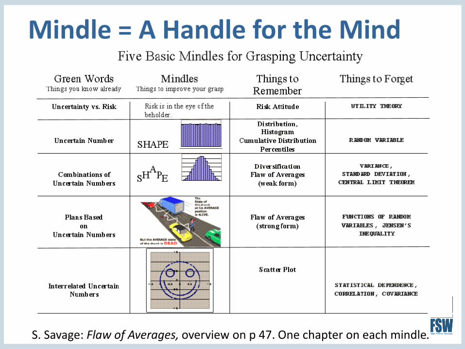
Mindle = A Handle for the Mind
S. Savage: Flaw of Averages, overview on p 47. One chapter on each mindle.

Save the date
Click on hyperlink below
http://events.r20.constantcontact.com/register/event?oeidk=a07eb2lk97u9fd05b26&llr=lr9yi7pab
Use the Super Super Secret code ANTE246 for a discount on your registration fee.
Building Better Water Rates for an Uncertain World
Thomas W. Chesnutt, Ph.D., CAP®A & N Technical Services, Inc.http://www.antechserv.com
839 Second Street, Suite 5Encinitas CA, 92024


