22
The Evolution of Industrial Clusters {
Simulating Spatial Dynamics
Thomas Brennery
Max-Planck-Institute for Research into Economic Systems
Evolutionary Economics Unit
Kahlaische Str. 10
07745 Jena, Germany
Niels Weigeltz
Max-Planck-Institute for Research into Economic Systems
Evolutionary Economics Unit
Kahlaische Str. 10
07745 Jena, Germany
ABSTRACT . Industrial clusters have received much attention in economic
research in the last decade. They are seen as one of the reasons for the eco-
nomic success of certain regions in comparison to others. This paper studies
the evolution of such industrial clusters. To this end, a spatial structure of re-
gions is set up and the entry, exit, and growth of �rms within these regions is
modelled and studied with the help of simulations. We are able to obtain some
knowledge about the basic characteristics of this dynamic process and about
the spatial relation between industries that results. It is shown that it matters
whether one or the other industry appears �rst and that location of clusters
of one industry in uence the location of other industries. Furthermore, some
necessary conditions for the evolution of industrial clusters are identi�ed.
KEYWORDS : evolution, industrial clusters, technological spillovers, simula-
tions, spatial agglomeration.
y Author to whom correspondence should be addressed.z We want to thank Ulrich Witt, Guido B�unstorf and the participants of the 'Industrial
District'-seminar and the workshop 'Economics Dynamics from a Physical View' for theirhelpful comments and discussions and the German federal ministry for education and researchfor �nancial support. The usual disclaimer applies.
2 Thomas Brenner and Niels Weigelt
1. Introduction
Previously regional phenomenon have gained much attention within economics.
Especially the question why certain regions are economically successful while oth-
ers are not has been increasingly frequently discussed. The theoretical discussion
of this phenomenon was triggered by various case studies of successful regions,
like Silicon Valley, the Third Italy and many more (such case studies can, for ex-
ample, be found in Rosegrant & Lampe 1992, Saxenian 1994, and Dalum 1995).
On the basis of these case studies several authors have attempted to explain the
speci�c reasons for the success of each of these regions. Furthermore, some gen-
eral concepts have been developed and various mechanisms have been identi�ed
that are seen as the causes for the success of those regions. The four main con-
cepts are those of industrial districts, industrial clusters, innovative milieux and
regional innovative systems (descriptions can be found in Becattini 1990, Maillat
& Lecoq 1992, Pyke & Sengenberger 1992, Scott 1992, Camagni 1995, van Dijk
1995, Markusen 1996, Lawson 1997, Rabellotti 1997; an attempt to structure
these approaches can be found in Brenner 2000).
Although the literature on industrial districts and the likes has increased and is
still increasing tremendously, most of the literature addresses the reasons for the
success of such regional systems and does not deal in general with the question,
how these spatial structures come into existence. In most of the case studies this
question is addressed for the speci�c situation of the region that is studied. In
the case of Third Italy historical aspects that led to an entrepreneurial spirit,
a trustful atmosphere and helpful politics are suggested to be the determinants
(cf. Dei Ottati 1994 and Rabellotti 1997). In the case of Route 128 research
funds from the Department of Defence are seen as the initial driving force (cf.
Rosegrant & Lampe 1992). While in the case of North Jutland a mixture of a wise
creation of new institutes at the Aalborg university, the existence of a �rm with
experience in the relevant �eld and the change of the market are regarded to be
the crucial factors for the evolution of this district (cf. Dalum 1995). Many other
examples could be listed here { all with very speci�c explanations for speci�c
developments.
The theoretical literature can be divided into two nearly separate strands. One
is based on the above cited case studies and tries to identify general mechanisms
that make local systems successful without considering the question of how these
mechanisms started. The other is based on the empirical �nding that economic
activity, on a general and an industrial level, is concentrated (see for example
the calculation of gini-coe�cients in Krugman 1991a and the calculation of an
index of geographic concentration in Ellison & Glaeser 1994). With respect to
the latter, several theoretical approaches have been able to rebuild concentration
in simulations (cf. for example Camagni & Diappi 1991 and Jonard & Yildizoglu
1998). However, the aim of these studies was to obtain a structure of spatial
distribution that is similar to the one observed in reality. They focus on the
�nal distribution of economic activity. Thus, a theoretical approach that deals
on a general level with the questions of how, where and when industrial clusters
evolve is missing. This paper makes a �rst step to �ll this gap. The major aim is
to model the dynamics that lead to the evolution of industrial clusters. Through
this, some �rst answers to the above questions are obtained.
The Evolution of Industrial Clusters 3
The approach proposed here is based on simulating the spatial dynamics of
two industries using �rst a number of unconnected region. After the analysis of
some basic aspects a cellular automaton is developed. This means that a two-
dimensional space is divided into small quadratic units. This allows to deal with
local interactions, both within a unit and between neighbouring units. Similar
approaches are used in the literature on economic agglomeration (cf. Camagni
& Diappi 1991, Krugman 1991b, Allen 1997a and 1997b, Schweitzer 1998, and
Cani�els & Verspagen 1999) and industrial concentration (cf. Jonard & Yildizoglu
1998). However, the present approach deviates from these approaches in its aims
and two structural aspects. The aim is to understand the evolution of industrially
specialised regions in the context of a changing global environment. Instead of
reproducing the distribution of economic agglomeration, this paper focuses on
the change of the distribution of industrial activity and its path-dependency. To
this end, two aspects have to be treated in more detail than it is done in the
literature on agglomerations. First, the interaction between industries has to be
explicitly modelled considering di�erent courses of exogenous changes. Second,
the processes within each geographical unit are modelled in detail, concerning
the entry of �rms, their growth and eventually their exit. The details of this are
outlined in the next section.
The structural analysis by T. Brenner (2000) has shown that di�erent mecha-
nisms play a role during the evolution of an industrial cluster or milieu. Modelling
all of them simultaneously would cause a simulation approach to be too complex
to interpret the di�erent results. Thus, it seem to be more adequate to restrict
the modelling in each approach to one class of industrial cluster or milieu, so that
the impact of each mechanism can be understood in detail. Finally the di�erent
mechanisms can be put together to get a comprehensive view of their complex
interaction. This paper is restricted to two mechanisms. The �rst mechanism
are knowledge spillovers between �rms of the same and of di�erent industries
and the local stickiness of these spillovers (for empirical aspects on this see Ja�e,
Trajtenberg & Henderson 1992 and Audretsch 1998). The second mechanism are
the local aspects of the founding of new enterprises. Both aspects have been iden-
ti�ed to be major aspects of the evolution of industrial clusters and innovative
milieux (cf. Brenner 2000).
The paper proceeds as follows. In Section two the basic model is developed.
Section three focuses on a case with �ve spatially independent regions. The dy-
namics found in simulations are analysed with respect to the concentration of
industries within one or several regions and with respect to the spatial relation
and spillovers between industries. In Section four the model is expanded to situa-
tion with 49 regions that are located on a 7�7 grid and where spillovers between
and spin-o�s in neighbouring regions occur. The impact of these two aspects on
the spatial distribution of two industries are studied and discussed. Section �ve
concludes.
4 Thomas Brenner and Niels Weigelt
2. Basic model
2.1. Dynamics of firms
The basic elements of the model are �rms. The number of �rms is endogenously
given since we allow for the entry and exit of �rms. The state of each �rm is
characterised by several variables which all change endogenously. Furthermore,
several parameters are de�ned that determine the behaviour of �rms and there
surrounding. These parameter are given exogenous and their in uence on the
spatial distribution of industrial activity is studied below.
The variables that de�ne the state of a �rm n (2 N (t)) at time t (t 2
f0; 1; 2; :::g) are its capital Kn(t), its labour force Ln(t), its technology Tn(t),
and its liquidity Bn(t). Furthermore, each �rm is assigned to a region qn (2 Q)
and an industry in (2 I) which cannot be changed during the life of a �rm.
The production function of a �rm is assumed to depend on its attributesKn(t),
Ln(t), and Tn(t). Besides these usual determinants technological spillovers from
other �rms are assumed to in uence the production capacity. These spillovers
are the only kind of positive local external economies that are considered here.
All other aspects of agglomeration economies that are discussed in the litera-
ture are excluded in this approach in order to restrict the model to a few local
mechanisms. Thus, the model developed here is adequate only for analysing the
evolution of technological clusters where �rms pro�t from technological spillovers
from other �rms located in the same or neighbouring regions. Industrial clusters
or districts which are based on vertical and horizontal contacts and co-operations
are not adequately represented by this approach. Furthermore, this approach
does not deal with the labour market in detail. It concentrates on the evolution
of a local system that has been called technological cluster elsewhere (cf. Brenner
2000).
Spillovers are bound with respect to location and industry. Therefore, we de�ne
a value Sq;i(t) which denotes the spillovers that a �rm belonging to industry i at
location q can pro�t from. The value of Sq;i(t) is discussed below in detail. The
spillovers and the technological state Tn(t) of a �rm determine the steepness of
the production function. With respect to the production factorsKn(t) and Ln(t)
a Cobb-Douglas production function is assumed here, so that the output Yn(t)
of �rm n of industry i in region q is given by
Yn(t) =hTn(t)
i � Sq;i(t)i�Kn(t)
�i � Ln(t)�i : (2.1)
The partial output elasticities �i and �i are parameters that are identical for all
�rms of the same industry. They may, however, di�er between industries. The
same holds for i.
It is assumed here that �rms are not able to in uence their technology Tn(t)
and the amount of spillovers Sq;i(t). This means that the possibility to vary the
amount of R&D-expenditures is neglected. All �rms of one industry are assumed
to spend the same amount on R&D and, therefore, have the same probability
to improve their technology. Whether a �rm n is able to improve its technology
at time t is a random event. With a probability pI;i a �rm of industry i is
assumed to innovate at time t, which improves its technology by 0:01. Thus,
each improvement is an incremental step. The impact of this incremental step,
The Evolution of Industrial Clusters 5
however, is assumed to decrease with the value of the technology Tn(t) that is
already reached. Therefore, the value Tn(t) i enters the production function with
0 < i < 1.
The amount of capital Kn(t) and labour Ln(t) that are used in the produc-
tion process are chosen by the �rm. To this end, the optimal factor inputs are
calculated at each time for a given demand. The �rms are assumed not to be
able to predict the demand they face in the next period. Therefore, they take the
average of the demands at the present and the previous time as an approxima-
tion for the demand they should expect in the next period, which is denoted by
D̂n(t). Similarly, they assume wages, spillovers and their technology to remain
constant. Thus, the optimal capital and labour inputs are
Kn;opt(t) =
D̂n(t) � wq(t� 1)�i � �
�i
i
��i
i� r�i � Tn(t� 1) i � Sq;i(t� 1)
! 1�i+�i
(2.2)
and
Ln;opt(t) =
D̂n(t) � r
�i � ��i
i
��i
i� wq(t� 1)�i � Tn(t� 1) i � Sq;i(t� 1)
! 1�i+�i
(2.3)
where wq(t) denotes the wage rate in region q at time t and r is the interest rate
on the capital market.
However, �rms do not always change their capital and labour input to the
optimal value within one period. The expansion of capital is costly and takes time
and capital investment is in general irreversible, while labour has to be hired and
in some cases trained. Thus, it is assumed that capital increases by maximally
5% and decreases by maximally 10% each period. Furthermore, investment also
depends on the liquidity Bn(t) of a �rm and is assumed to be determined in the
following way. First, set Kn;#(t) = 0:9 �Kn(t� 1) and Kn;"(t) = 1:05 �Kn(t� 1).
Then,
Kn(t)�Kn(t�1) =
8>>>>><>>>>>:
�0:1 �Kn(t� 1) if Kn;opt(t) < Kn;#(t)
Kn;opt(t)�Kn;#(t)
1+exp
hBn(t)
Kn;opt(t)�Kn;#(t)
i if Kn;#(t) < Kn;opt(t) < Kn;"(t)
Kn;"(t)�Kn;#(t)
1+exp
hBn(t)
Kn;"(t)�Kn;#(t)
i if Kn;opt(t) > Kn;"(t)
:
(2.4)
This equation is arbitrarily chosen to re ect the fact that the higher the liquidity
of a �rm, the more money it will invest up to the level which is optimal and
possible.
The amount of labour employed is assumed to be chosen such that the marginal
factor productivity is the same for capital and labour. Again changes are re-
stricted to a maximum of 50% of the previous labour input. However, since the
labour input is related to the capital input, the dynamics of capital and labour
inputs are in general limited by the restrictions on the changes of capital. Ln(t)
is always a natural number representing the number of employees.
The liquidity of �rms is updated each period by subtracting the money invested
(Kn(t)�Kn(t�1)), the costs of capital (r �Kn(t)), the labour costs (wq(t)�Ln(t)),
6 Thomas Brenner and Niels Weigelt
and the �xed costs Fi and adding the returns from selling the good on the market
(Pn(t) �Dn;s(t)). The �xed costs are an industry-speci�c parameter. Pn(t) and
Dn;s(t) are described in detail below.
Firms are assumed to be price setters. As outlined above �rms adapt their
production to the demands they face. The price is set according to a mixture
of markup-pricing and an orientation towards the market price. To use mark-up
pricing, the costs of production have to be calculated. The average costs are
cn(t) =Fi + r �Kn(t) + wq(t) � Ln(t)
Yn(t): (2.5)
The price Pn(t) charged by �rm n at time t is assumed to be given by
Pn(t) = �i � (1 +mi) � cn(t) + (1� �i) � �P (t� 1) (2.6)
where �i and mi are industry-speci�c parameters and �P (t) is the average price
for which the good is traded on the market, which is called the market price in
this approach. mi is the mark-up used in industry i, while �i determines how
much �rms stick to the price resulting from the mark-up rule instead of orienting
on the market price. The calculation of the market price is given in Equation
(2.10).
2.2. Entry and exit of firms
Firms are removed either if they employ only one worker (this threshold is
chosen for convenience) or if their liquidity falls below a certain trash-hold Bmin.
New �rms occur due to two processes: random entry and spin-o�s. First, with
a constant probability pF;q a �rm enters at any time t for any industry (this
probability may vary between regions). Such a �rm starts with an initial set of
variables given by Kinit, Linit, and Binit. The initial value of Tn is determined
by calculating the average value of T~n(t) for all �rms ~n that belong to the same
industry. To this average value an amount of either 0, 0:01 or 0:02 is added with
equal probability. This can be interpreted as follows. From time to time someone
has, starting from the average technological standard, an innovative idea and
founds a new �rm to exploit this idea.
Second, within a region with a probability, depending on the number of �rms
that belong to a certain industry and are located in this region, a spin-o� �rm
is founded. The probability for such a spin-o� is given by
Ni;q � pS;q
Ni;q � pS;q � pS;q + 1(2.7)
where Ni;q denotes the number of �rms in region q that belong to industry i and
pS;q is a parameter, dependent on the region. A spin-o� �rms starts with the
same initial variables as de�ned above, namely Kinit, Linit, and Binit, except for
the technology. To determine the technology of a spin-o� �rm, one of the �rms of
the same industry in the region is chosen randomly. The spin-o� �rm is assumed
to be a spin-o� of this �rm and, therefore, imitates the technology of this �rm.
Again either 0, 0:01, or 0:02 is added with equal probability, representing the
fact that the spin-o� �rm might innovate right at the beginning.
The Evolution of Industrial Clusters 7
2.3. Technological spillovers
In empirical studies it has been repeatedly shown that �rms pro�t a lot from
spillovers from other �rms. These spillovers have been shown to be to some extend
a localised phenomenon (cf. Ja�e, Trajtenberg & Henderson 1992 and Audretsch
1998). Therefore, we consider local spillovers between �rms in this approach. In
a �rst approach in Section 3 spillovers are assumed to occur only within regions.
In Section 4 we will also allow for spillovers between neighbouring regions. With
respect to industries, inter-industrial spillovers are explicitly considered. The
amount of spillovers within and between industries is denoted in the form of a
spillover matrix (sij)i;j2I . The total spillover that a �rm of industry i in region
q pro�ts from is de�ned by
Sq;i =h X
n2N(t)
qn=q
siin � Tn(t)i�i
: (2.8)
The in uence of this spillover on the production function of each �rm is given
above in Equation (2.1).
2.4. Labour market
Labour markets are assumed to be local in this approach. This means that we
exclude any kind of movement of the labour force. Thus, a �rm can only employ
people from the region where itself is located in. Wages result to be variables of
the regions. A di�erentiation of the labour market with respect to industries is
not considered. The wage rate wq(t) within a region is assumed to be given by
wq(t) = wq;0 �
264 X
n2N(t)qn=q
Ln(t) + Lq;other
375 (2.9)
where wq;0 is a parameter determining the basic wage level in region q and
Lq;other is a parameter denoting the labour demand of all other industries in
region q that are not explicitly considered in the model. The labour demand of
all other industries is assumed to remain constant. This parameter determines
whether wages react more or less strongly to changes in the labour demand of
the explicitly modelled �rms.
2.5. Market and firm-specific demand
All �rms of one industry are assumed to produce the same kind of good.
Thus, they supply the same market and compete on this market. However, it is
assumed that the goods are not identical, so that they are substitutable but not
all customers will choose automatically the most inexpensive good.
Hence, to calculate the demand for each �rm n, two steps are necessary. First,
the overall demand has to be determined. Then, this demand has to be dis-
tributed between the �rms of the respective industry. Demand is assumed to be
global, so that no distinction with respect to the locality of �rms is necessary.
The overall demand for one kind of good is assumed to depend on the average
8 Thomas Brenner and Niels Weigelt
price of the good, which was above called the market price. The average price
for the good of industry i is given by
�Pi(t) =X
n2N(t)
in=i
[Dn;s(t� 1) � Pn(t)] (2.10)
where for each �rm the number of sold goodsDn;s(t�1) in the last period is used
to avoid a circular de�nition of demands. The market demand �Di(t) is assumed
to be given by
�Di(t) =�Di;0
�Pi(t)(2.11)
where Di;0 is an industry-speci�c parameter.
The market demand �Di(t) is distributed between the �rms of industry i ac-
cording to their prices. The higher the price of a �rm the smaller the demand
for the good produced by this �rm will be. However, since we assume that goods
are not identical, �rms with higher prices will still sell some pieces of the good,
at least if their prices are not too high. To model these characteristics, a market
share factor Mn(t) is de�ned for each �rm n by
Mn(t) =
8<:
�in ��Pin (t)
Pn(t)� 1 if
Pn(t)�Pin (t)
< �in
0 ifPn(t)�Pin (t)
> �in
(2.12)
where �in is a industry-speci�c parameter, which determines how much �rms are
able to charge for the good without being neglected by the customers. All �rms
with a price above �i � �Pin(t) do not sell any piece of the good. Below this value
the demand for a �rm's good decreases with its price. The demand for the good
of �rm n is calculated according to
Dn(t) =Mn(t) � �Din
(t)P~n2N(t)
i~n=in
M~n(t): (2.13)
This Dn(t) equals the number of goods Dn;s(t) that are sold by the �rm if the
�rm is able to produce enough goods. If it is not able to do so, the number of
goods sold equals the possible output, meaning Dn;s(t) = Y (t).
3. Analysis of simulations with independent regions
Before we analyse a model with a spatial distribution of regions and spillovers
between neighbouring regions, the above model will be simulated and analysed
for �ve independent regions and two industries. Through this the in uence of all
parameters is studied in detail. The analysis of the more complex spatial setting
in the next section can then be restricted to those parameters that in uence the
spatial distribution of industrial activity.
The study of �ve independent regions proceeds in four steps. Firstly, the ini-
tial dynamics of the simulations are discussed. Secondly, a sensitivity analysis is
conducted for all parameters. Thirdly, the parameters that cause �rms to agglom-
erate in one or a few regions are analysed and discussed. Finally, the implications
of a successive introduction of industries are analysed.
The Evolution of Industrial Clusters 9
3.1. Initial dynamics
In the following sensitivity analysis we study the impact of all parameters on
the �nal distribution of �rms and employment. However, before such an analysis
is conducted we have to study what '�nal' means and how the dynamics in the
simulations look like. To this end the initial dynamics for all parameter sets that
have been used, are studied.
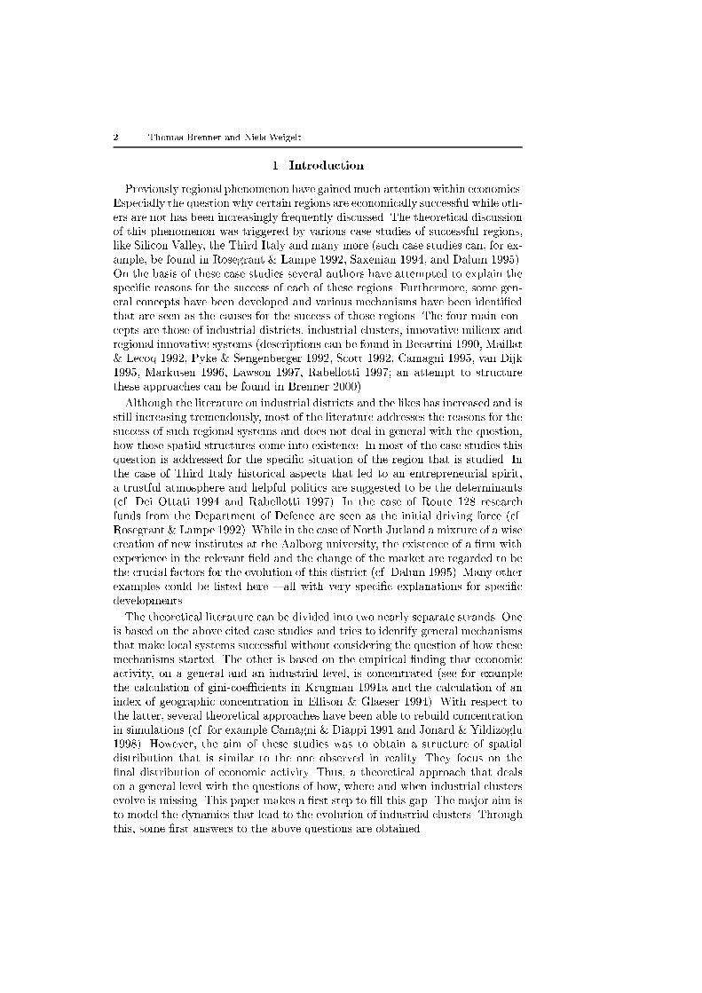
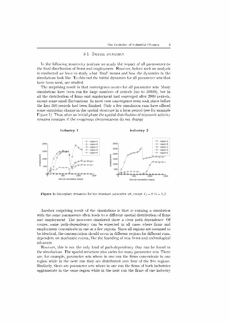
The surprising result is that convergence occurs for all parameter sets. Many
simulations have been run for large numbers of periods (up to 10000), but in
all the distribution of �rms and employment had converged after 2000 periods,
except some small uctuations. In most case convergence even took place before
the �rst 500 periods had been �nished. Only a few simulation runs have o�ered
some surprising change in the spatial structure in a later period (see for example
Figure 1). Thus, after an initial phase the spatial distribution of economic activity
remains constant if the exogenous circumstances do not change.
industry 1
0 500 1000 15000
500
1000
1500
2000 region A region B region C region D region E
empl
oym
ent
time [in simulation steps]
industry 2
0 500 1000 15000
500
1000
1500
2000
2500
3000 region A region B region C region D region E
emp
loym
ent
time [in simulation steps]
Figure 1: Exemplary dynamics for the standard parameter set, except Fi = 0 8i = 1; 2.
Another surprising result of the simulations is that re-running a simulation
with the same parameters often leads to a di�erent spatial distribution of �rms
and employment. The processes simulated show a clear path-dependence. Of
course, some path-dependency can be expected in all cases where �rms and
employment concentrate in one or a few regions. Since all regions are assumed to
be identical, the concentration should occur in di�erent regions for di�erent runs,
dependent on stochastic events, like the founding of new �rms and technological
advances.
However, this is not the only kind of path-dependency that can be found in
the simulations. The spatial structure also varies for many parameter sets. There
are, for example, parameter sets where in one run the �rms concentrate in one
region while in the next run they are distributed over four of the �ve regions.
Similarly, there are parameter sets where in one run the �rms of both industries
agglomerate in the same region while in the next run the �rms of one industry
10 Thomas Brenner and Niels Weigelt
are distributed over three regions and the �rms of the other industry agglomerate
in another region. There are plenty of such results. There seems to be no stable
distribution for many of the parameter sets. Thus, path-dependency does not
only occur with respect to the regions where �rms agglomerate, but also with
respect to the number of regions that contain an agglomeration and the spatial
relation between industries. This path-dependence has important implications
for the dynamics of local systems which will be discussed in more detail at the
end of this section.
3.2. Sensitivity analysis for all parameters
We will neglect the initial dynamics during the sensitivity analysis. Instead,
we study for each parameter whether the parameter has an in uence on the �-
nal distribution of �rms and employment. To this end, the �nal state has to be
characterised by some well-de�ned aspects. Four aspects are used here: 1) the
number of regions that contain a signi�cant number of employment of an indus-
try, denoted by Qs, 2) the share of those regions that contain also a signi�cant
number of employment of the other industry, denoted by Qd, 3) the total number
of employment, denoted by L and 4) the total number of �rms, denoted by N .
The aim of the sensitivity analysis is to identify for each parameter the aspects
that are in uenced by the parameter. Therefore, each parameter is varied in both
directions and a statistical analysis of the resulting changes of Qs, Qd, L, and
N is conducted. Before this can be done, a standard parameter set has to be de-
�ned. We have chosen this parameter set such that it leads to some intermediate
results according to the aspects above, meaning that there is neither a complete
concentration on one region nor an equal distribution of the employment over
all region and that there is neither a strict separation of the two industries nor
a strict coexistence. This standard parameter set is given by �i = 0:5, �i = 0:5,
i = 0:4, �i = 0:4, pI;i = 0:1, Fi = 1, r = 0:1, mi = 0:05, �i = 0:7, Bmin = �10,
pF;q = 0:1, pS;q = 0:02, Kinit = 5, Linit = 5, Binit = 10, sii =13 , sij =
19 8i 6= j,
wq;0 = 0:0001, Lq;other = 1000, �Di;0 = 2000, and �i = 1:5. Furthermore, the
simulations are started in the standard case with no �rms existing and an initial
value of technology of Tinit = 1. The spillovers for each region and industry are
set to Sq;i = 0:5 if no corresponding �rm exists. The results of the sensitivity
analysis are given in Table 1.
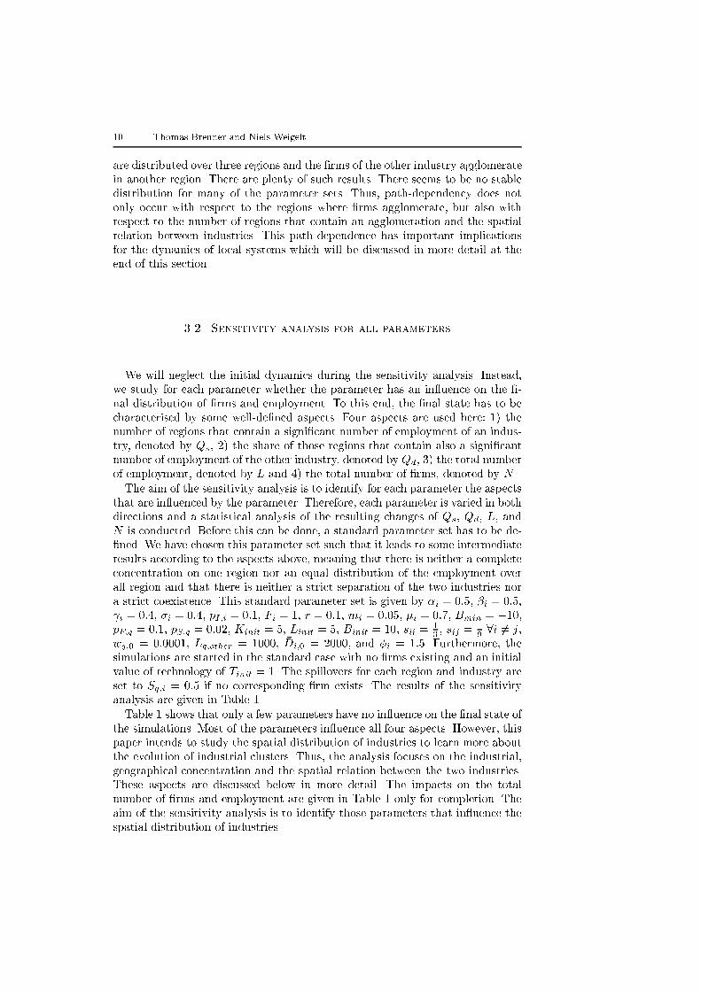
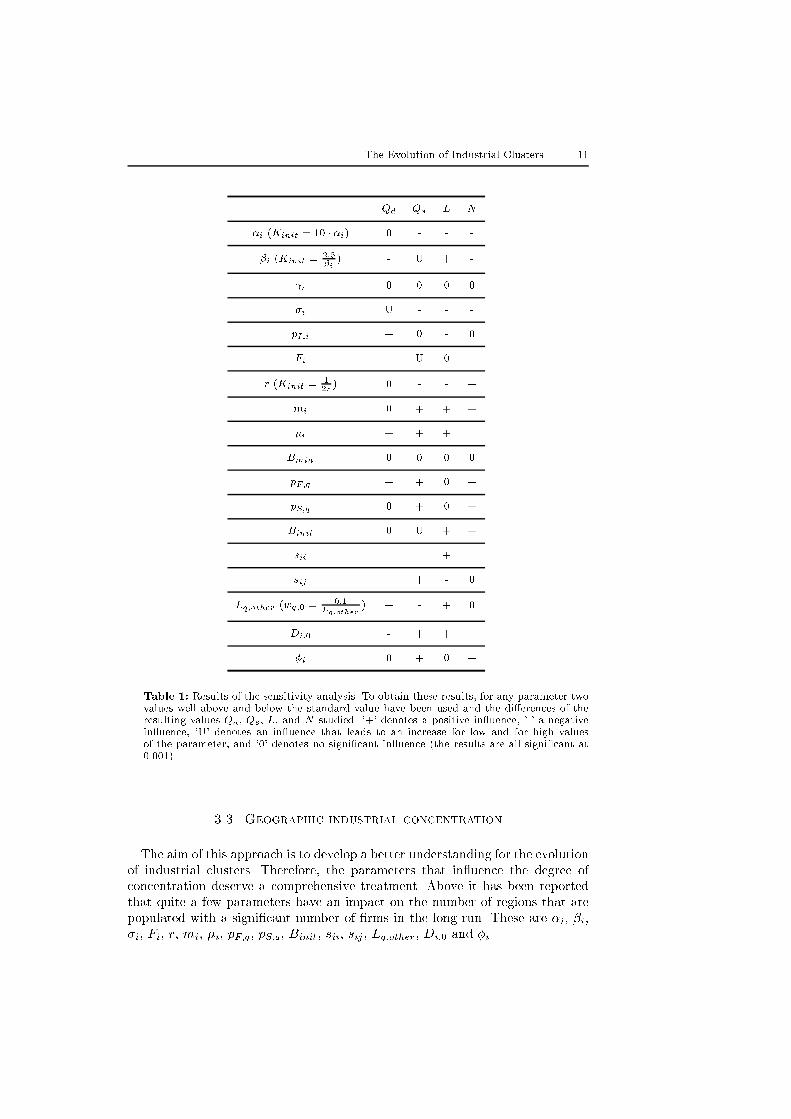
Table 1 shows that only a few parameters have no in uence on the �nal state of
the simulations. Most of the parameters in uence all four aspects. However, this
paper intends to study the spatial distribution of industries to learn more about
the evolution of industrial clusters. Thus, the analysis focuses on the industrial,
geographical concentration and the spatial relation between the two industries.
These aspects are discussed below in more detail. The impacts on the total
number of �rms and employment are given in Table 1 only for completion. The
aim of the sensitivity analysis is to identify those parameters that in uence the
spatial distribution of industries.
The Evolution of Industrial Clusters 11
Qd Qs L N
�i (Kinit = 10 � �i) 0 - - -
�i (Kinit =2:5�i
) - U + -
i 0 0 0 0
�i U - - -
pI;i + 0 - 0
Fi - U 0 -
r (Kinit =1
2r) 0 - - +
mi 0 + + +
�i + + + -
Bmin 0 0 0 0
pF;q + + 0 +
pS;q 0 + 0 +
Binit 0 U + +
sii - - + -
sij + + - 0
Lq;other (wq;0 =0:1
Lq;other) + - + 0
�Di;0 - + + +
�i 0 + 0 +
Table 1: Results of the sensitivity analysis. To obtain these results, for any parameter twovalues well above and below the standard value have been used and the di�erences of theresulting values Qd, Qs, L, and N studied. '+' denotes a positive in uence, '-' a negativein uence, 'U' denotes an in uence that leads to an increase for low and for high valuesof the parameter, and '0' denotes no signi�cant in uence (the results are all signi�cant at0.001).
3.3. Geographic industrial concentration
The aim of this approach is to develop a better understanding for the evolution
of industrial clusters. Therefore, the parameters that in uence the degree of
concentration deserve a comprehensive treatment. Above it has been reported
that quite a few parameters have an impact on the number of regions that are
populated with a signi�cant number of �rms in the long run. These are �i, �i,
�i, Fi, r, mi, �i, pF;q, pS;q, Binit, sii, sij , Lq;other, �Di;0 and �i.
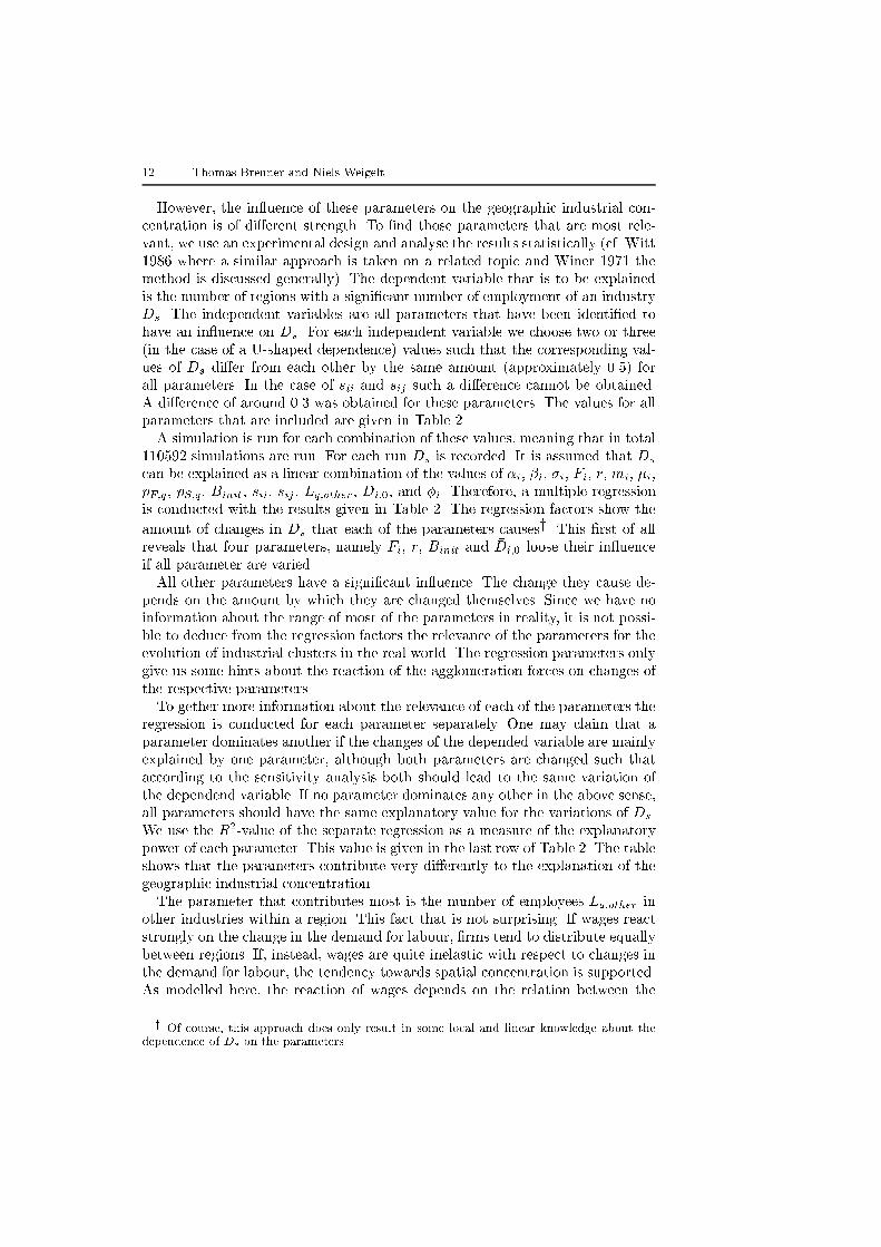
12 Thomas Brenner and Niels Weigelt
However, the in uence of these parameters on the geographic industrial con-
centration is of di�erent strength. To �nd those parameters that are most rele-
vant, we use an experimental design and analyse the results statistically (cf. Witt
1986 where a similar approach is taken on a related topic and Winer 1971 the
method is discussed generally). The dependent variable that is to be explained
is the number of regions with a signi�cant number of employment of an industry
Ds. The independent variables are all parameters that have been identi�ed to
have an in uence on Ds. For each independent variable we choose two or three
(in the case of a U-shaped dependence) values such that the corresponding val-
ues of Ds di�er from each other by the same amount (approximately 0.5) for
all parameters. In the case of sii and sij such a di�erence cannot be obtained.
A di�erence of around 0.3 was obtained for these parameters. The values for all
parameters that are included are given in Table 2.
A simulation is run for each combination of these values, meaning that in total
110592 simulations are run. For each run Ds is recorded. It is assumed that Ds
can be explained as a linear combination of the values of �i, �i, �i, Fi, r, mi, �i,
pF;q, pS;q, Binit, sii, sij , Lq;other, �Di;0, and �i. Therefore, a multiple regression
is conducted with the results given in Table 2. The regression factors show the
amount of changes in Ds that each of the parameters causesy. This �rst of all
reveals that four parameters, namely Fi, r, Binit and �Di;0 loose their in uence
if all parameter are varied.
All other parameters have a signi�cant in uence. The change they cause de-
pends on the amount by which they are changed themselves. Since we have no
information about the range of most of the parameters in reality, it is not possi-
ble to deduce from the regression factors the relevance of the parameters for the
evolution of industrial clusters in the real world. The regression parameters only
give us some hints about the reaction of the agglomeration forces on changes of
the respective parameters.
To gether more information about the relevance of each of the parameters the
regression is conducted for each parameter separately. One may claim that a
parameter dominates another if the changes of the depended variable are mainly
explained by one parameter, although both parameters are changed such that
according to the sensitivity analysis both should lead to the same variation of
the dependend variable. If no parameter dominates any other in the above sense,
all parameters should have the same explanatory value for the variations of Ds.
We use the R2-value of the separate regression as a measure of the explanatory
power of each parameter. This value is given in the last row of Table 2. The table
shows that the parameters contribute very di�erently to the explanation of the
geographic industrial concentration.
The parameter that contributes most is the number of employees Lq;other in
other industries within a region. This fact that is not surprising. If wages react
strongly on the change in the demand for labour, �rms tend to distribute equally
between regions. If, instead, wages are quite inelastic with respect to changes in
the demand for labour, the tendency towards spatial concentration is supported.
As modelled here, the reaction of wages depends on the relation between the
y Of course, this approach does only result in some local and linear knowledge about thedependence of Ds on the parameters.
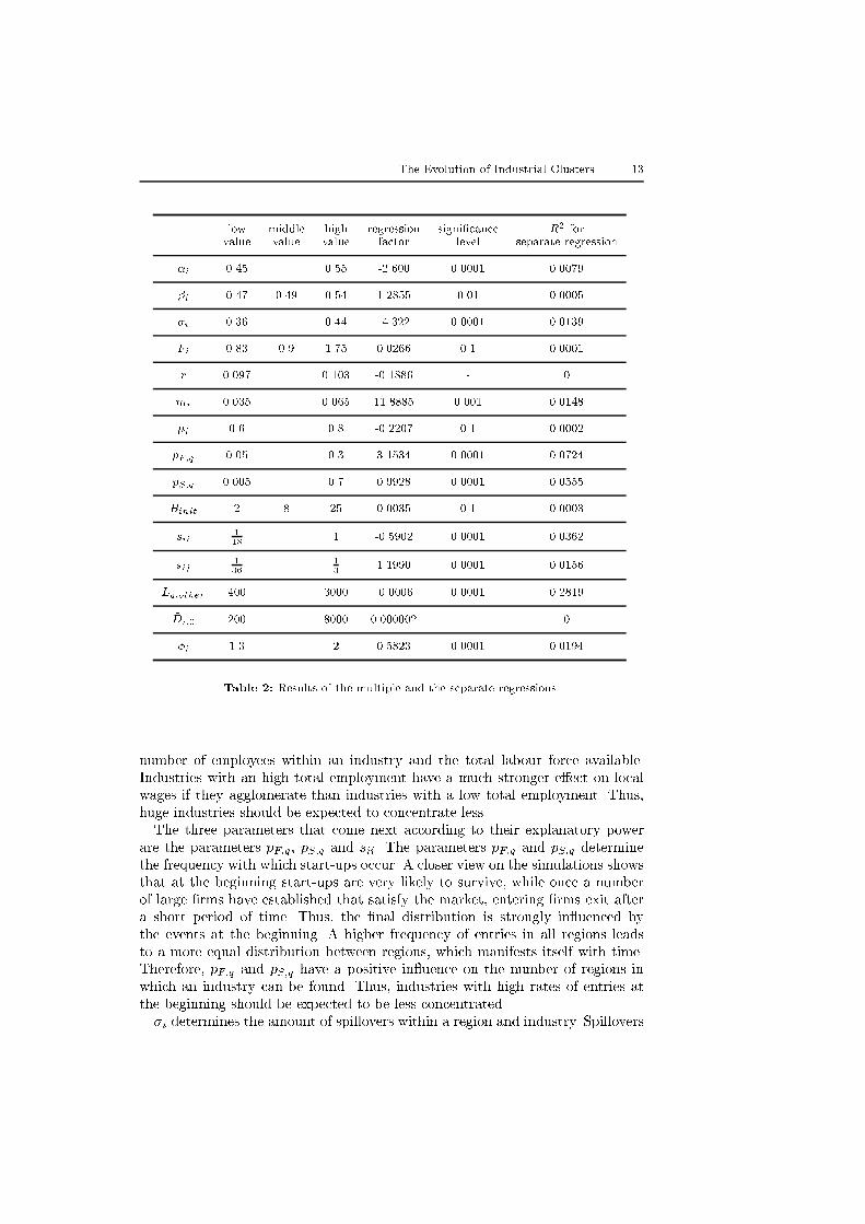
The Evolution of Industrial Clusters 13
low middle high regression signi�cance R2 forvalue value value factor level separate regression
�i 0.45 0.55 -2.600 0.0001 0.0079
�i 0.47 0.49 0.54 1.2855 0.01 0.0005
�i 0.36 0.44 -4.322 0.0001 0.0139
Fi 0.83 0.9 1.75 0.0266 0.1 0.0001
r 0.097 0.103 -0.1886 - 0
mi 0.035 0.065 11.8885 0.001 0.0148
�i 0.6 0.8 -0.2207 0.1 0.0002
pF;q 0.05 0.3 3.1534 0.0001 0.0724
pS;q 0.005 0.7 0.9928 0.0001 0.0555
Binit 2 8 25 0.0035 0.1 0.0003
sii1
181 -0.5902 0.0001 0.0362
sij1
36
1
31.1990 0.0001 0.0156
Lq;other 400 3000 -0.0006 0.0001 0.2819
�Di;0 200 8000 0.000002 - 0
�i 1.3 2 0.5823 0.0001 0.0194
Table 2: Results of the multiple and the separate regressions.
number of employees within an industry and the total labour force available.
Industries with an high total employment have a much stronger e�ect on local
wages if they agglomerate than industries with a low total employment. Thus,
huge industries should be expected to concentrate less.
The three parameters that come next according to their explanatory power
are the parameters pF;q, pS;q and sii. The parameters pF;q and pS;q determine
the frequency with which start-ups occur. A closer view on the simulations shows
that at the beginning start-ups are very likely to survive, while once a number
of large �rms have established that satisfy the market, entering �rms exit after
a short period of time. Thus, the �nal distribution is strongly in uenced by
the events at the beginning. A higher frequency of entries in all regions leads
to a more equal distribution between regions, which manifests itself with time.
Therefore, pF;q and pS;q have a positive in uence on the number of regions in
which an industry can be found. Thus, industries with high rates of entries at
the beginning should be expected to be less concentrated.
�i determines the amount of spillovers within a region and industry. Spillovers
14 Thomas Brenner and Niels Weigelt
are repeatedly supposed to be one of the most important reasons for economic ag-
glomerations in the literature. This study supports that view. The more spillovers
occur, the more economic activity will concentrate. Thus, industries where �rms
pro�t very much from spillovers should be spatially more concentrated than in-
dustries where �rms pro�t less from spillovers.
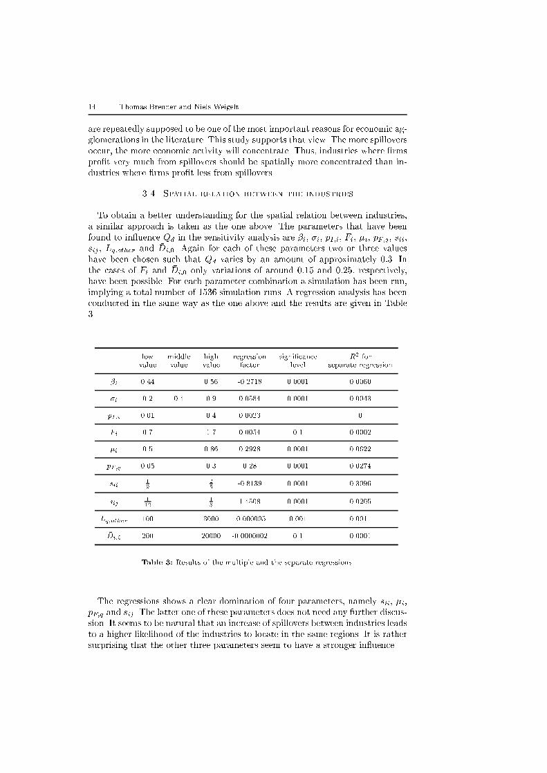
3.4. Spatial relation between the industries
To obtain a better understanding for the spatial relation between industries,
a similar approach is taken as the one above. The parameters that have been
found to in uence Qd in the sensitivity analysis are �i, �i, pI;i, Fi, �i, pF;q, sii,
sij , Lq;other and �Di;0. Again for each of these parameters two or three values
have been chosen such that Qd varies by an amount of approximately 0:3. In
the cases of Fi and �Di;0 only variations of around 0:15 and 0:25, respectively,
have been possible. For each parameter combination a simulation has been run,
implying a total number of 1536 simulation runs. A regression analysis has been
conducted in the same way as the one above and the results are given in Table
3.
low middle high regression signi�cance R2 forvalue value value factor level separate regression
�i 0.44 0.56 -0.2718 0.0001 0.0060
�i 0.2 0.4 0.9 0.0584 0.0001 0.0043
pI;i 0.01 0.4 0.0023 - 0
Fi 0.7 1.7 0.0054 0.1 0.0002
�i 0.5 0.86 0.2928 0.0001 0.0622
pF;q 0.05 0.3 0.28 0.0001 0.0274
sii1
9
2
5-0.8139 0.0001 0.3096
sij1
12
1
81.4508 0.0001 0.0205
Lq;other 100 3000 -0.000005 0.001 0.0011
�Di;0 200 20000 -0.0000002 0.1 0.0001
Table 3: Results of the multiple and the separate regressions.
The regressions shows a clear domination of four parameters, namely sii, �i,
pF;q and sij . The latter one of these parameters does not need any further discus-
sion. It seems to be natural that an increase of spillovers between industries leads
to a higher likelihood of the industries to locate in the same regions. It is rather
surprising that the other three parameters seem to have a stronger in uence.
The Evolution of Industrial Clusters 15
The domination of sii can be explained as follows. An increase of sii causes a
distribution of each industry over a large number of regions. Since the number
of regions has been restricted to �ve here, this means that the two industries
are not able any more to locate in di�erent regions. This aspect seems to be less
relevant in reality where much more than �ve locations exist.
The parameters �i and pF;q require are closer look at the dynamics of the sim-
ulations. pF;q, as has been discussed above, leads to a more equal distribution
of the industries between the regions, and therefore to a lower concentration of
the each industry and more local coincidences between the industries. A large
value of �i causes start-ups, which generally produce less e�cient than existing
�rms due the economies of scale, to charge prices much higher than the market
price. This decreases their likelihood to enter the market quickly after an ini-
tial phase. As a consequence, the situation becomes quite �xed after a shorter
period of time. This gives the concentration forces less time to operate and the
concentration of industries decreases. Hence, according to the argument above,
the probability of both industries to be located in the same region increases.
Again both mechanisms require a restricted number of regions to work properly.
Thus, the only parameter that can be expected to matter also in reality is sij .
3.5. Dynamics for the successive introduction of industries
Above it has been found that the spatial distribution of industries shows a
strong path-dependency. This implies that one should expect the resulting spa-
tial distribution to depend strongly on the temporal order of exogenous events.
Above all simulations have been run with both industries introduced right at
the beginning of the simulations. An alternative procedure would be to intro-
duce the industries one after the other. Due to the path-dependency it should be
expected that the results di�er signi�cantly between the situation where both
industries are introduced at the same time and the situation where one industry
is introduced later.
Therefore, we study such dynamics for �ve parameter sets. The �ve parameter
sets are chosen such that they represent di�erent types of spatial distributions,
in the case of a simultaneous introduction of the industries. This means that we
consider a parameter set where both industries always concentrate in one region
(standart parameter set except Lq;other = 10000), one where all regions contain
a signi�cant number of �rms of both industries (standard parameter set except
s12 = s21 = 13 and Lq;other = 100), one where both industries concentrate in
di�erent regions (standard parameter set except s12 = s21 =1100 and Lq;other =
10000), one where all regions are populated by only one industry (standard
parameter set except Lq;other = 100), and one where the results of the simulations
vary and are somewhere between the other four situations (standard parameter
set except s12 = s21 =29 ). With these parameter sets simulations were run where
the �rst industry is introduced right at the beginning of the simulation and the
second one is added after 1500 simulation step, after the spatial distribution for
the �rst industry has converged.
In the situations where both industries are concentrated in one region either
in the same or in two di�erent ones in the original setting, the successive intro-
duction of the industries does not change the results.
16 Thomas Brenner and Niels Weigelt
industry 1
0 500 1000 1500 2000 2500 30000
500
1000
1500
2000
2500
region A region B region C region D region E
empl
oym
ent
time [in simulation steps]
industry 2
0 500 1000 1500 2000 2500 30000
500
1000
1500
2000 region A region B region C region D region E
emp
loym
en
t
time [in simulation steps]
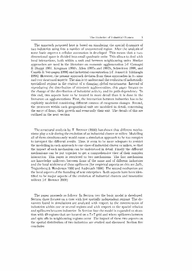
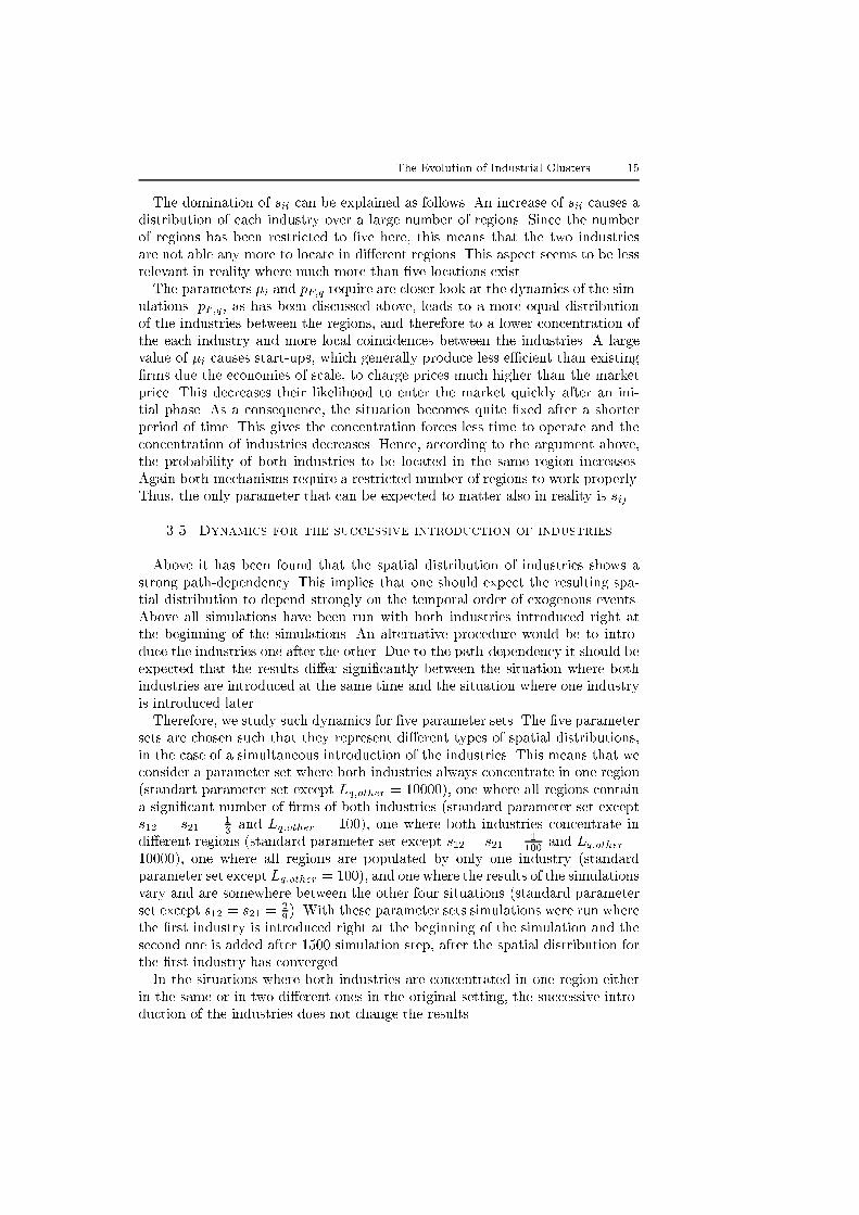
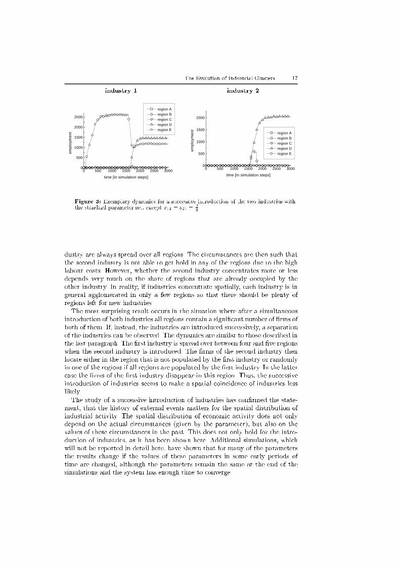
Figure 2: Exemplary dynamics for a successive introduction of the two industries withthe standard parameter set, except s12 = s21 =
2
9.
In the intermediate situation again the structure of the �nal distribution of
�rms varies a lot. However, it cannot be distinguished from the results of the
former simulations where both industries have been introduced at the same time.
Nevertheless, these simulations show how the introduction of the second industry
a�ects the spatial distribution of the �rst industry. If the second industry locates
in a region that contains already an agglomeration of the �rst industry it reduces
the labour demand of the �rst industry's �rms due to rising wages in the region
(see Figure 2). Thus, the location of a new industry in a region might have
a negative impact on the industry that is already located there. However, the
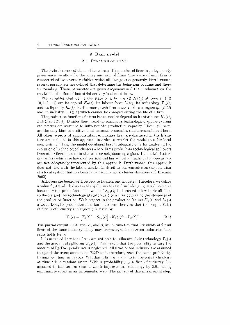
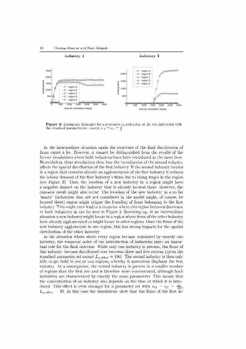
opposite result might also occur. The location of the new industry in a so far
'empty' (industries that are not considered in the model might, of course, be
located there) region might trigger the founding of �rms belonging to the �rst
industry. This might even lead to a situation where this region becomes dominant
in both industries as can be seen in Figure 3. Summing up, in an intermediate
situation a new industry might locate in a region where �rms of the other industry
have already agglomerated or might locate in other regions. Once the �rms of the
new industry agglomerate in one region, this has strong impacts for the spatial
distribution of the other industry.
In the situation where above every region became populated by exactly one
industry, the temporal order of the introduction of industries plays an impor-
tant role for the �nal outcome. While only one industry is present, the �rms of
this industry become distributed over between three and �ve regions (given the
standard parameter set except Lq;other = 100). The second industry is then only
able to get hold in one or two regions, whereby it sometimes displaces the �rst
industry. As a consequence, the second industry is present in a smaller number
of regions than the �rst one and is therefore more concentrated, although both
industries are characterised by exactly the same parameters. This means that
the concentration of an industry also depends on the time at which it is intro-
duced. This e�ect is even stronger for a parameter set with s12 = s21 = 1100 ,
Lq;other = 10. In this case the simulations show that the �rms of the �rst in-
The Evolution of Industrial Clusters 17
industry 1
0 500 1000 1500 2000 2500 30000
500
1000
1500
2000
2500
region A region B region C region D region E
empl
oym
ent
time [in simulation steps]
industry 2
0 500 1000 1500 2000 2500 30000
500
1000
1500
2000
region A region B region C region D region E
emp
loym
en
t
time [in simulation steps]
Figure 3: Exemplary dynamics for a successive introduction of the two industries withthe standard parameter set, except s12 = s21 =
2
9.
dustry are always spread over all regions. The circumstances are then such that
the second industry is not able to get hold in any of the regions due to the high
labour costs. However, whether the second industry concentrates more or less
depends very much on the share of regions that are already occupied by the
other industry. In reality, if industries concentrate spatially, each industry is in
general agglomerated in only a few regions so that there should be plenty of
regions left for new industries.
The most surprising result occurs in the situation where after a simultaneous
introduction of both industries all regions contain a signi�cant number of �rms of
both of them. If, instead, the industries are introduced successively, a separation
of the industries can be observed. The dynamics are similar to those described in
the last paragraph. The �rst industry is spread over between four and �ve regions
when the second industry is introduced. The �rms of the second industry then
locate either in the region that is not populated by the �rst industry or randomly
in one of the regions if all regions are populated by the �rst industry. In the latter
case the �rms of the �rst industry disappear in this region. Thus, the successive
introduction of industries seems to make a spatial coincidence of industries less
likely.
The study of a successive introduction of industries has con�rmed the state-
ment, that the history of external events matters for the spatial distribution of
industrial activity. The spatial distribution of economic activity does not only
depend on the actual circumstances (given by the parameter), but also on the
values of these circumstances in the past. This does not only hold for the intro-
duction of industries, as it has been shown here. Additional simulations, which
will not be reported in detail here, have shown that for many of the parameters
the results change if the values of these parameters in some early periods of
time are changed, although the parameters remain the same at the end of the
simulations and the system has enough time to converge.
18 Thomas Brenner and Niels Weigelt
4. Analysis of a spatial model
In the last section the regional agglomeration of industries has been intensively
studied under the assumption of technological spillovers that are restricted to
spillovers within regions. The aspect that technological spillovers have a spatial
dimension such that they also occur in a signi�cant amount between locations
that are near to each other (cf. Ja�e, Trajtenberg & Henderson 1992) has been
neglected. The impact of this aspect on the location of industries is studied in
this section. All other aspects of the spatial distribution of industries, like its
path-dependency, the determinants of industrial concentration and the dynam-
ics of the related processes, which have been discussed in the last section, are
neglected here. The analysis focuses on the impact of spillovers between neigh-
bouring regions on the spatial distribution of the industries.
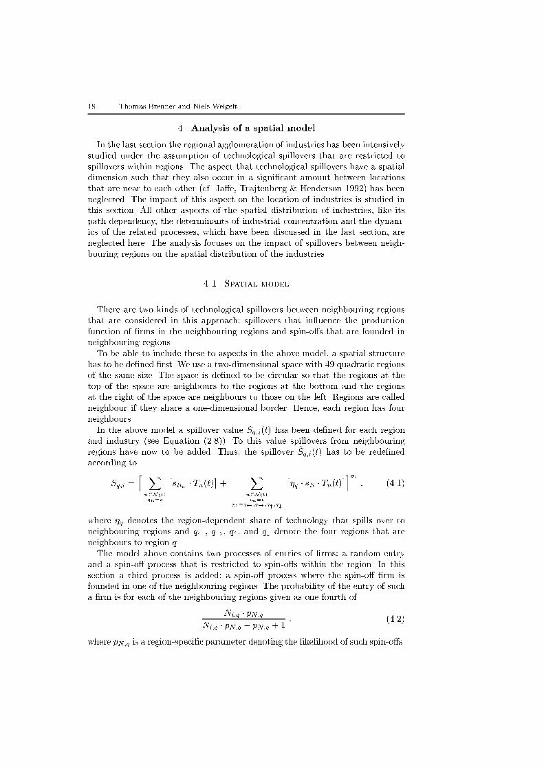
4.1. Spatial model
There are two kinds of technological spillovers between neighbouring regions
that are considered in this approach: spillovers that in uence the production
function of �rms in the neighbouring regions and spin-o�s that are founded in
neighbouring regions.
To be able to include these to aspects in the above model, a spatial structure
has to be de�ned �rst. We use a two-dimensional space with 49 quadratic regions
of the same size. The space is de�ned to be circular so that the regions at the
top of the space are neighbours to the regions at the bottom and the regions
at the right of the space are neighbours to those on the left. Regions are called
neighbour if they share a one-dimensional border. Hence, each region has four
neighbours.
In the above model a spillover value Sq;i(t) has been de�ned for each region
and industry (see Equation (2.8)). To this value spillovers from neighbouring
regions have now to be added. Thus, the spillover ~Sq;i(t) has to be rede�ned
according to
Sq;i =h X
n2N(t)qn=q
�siin � Tn(t)
�+
Xn2N(t)
in=iqn=q ;q!;q";q#
��q � sii � Tn(t)
�i�i: (4.1)
where �q denotes the region-dependent share of technology that spills over to
neighbouring regions and q , q!, q", and q# denote the four regions that are
neighbours to region q.
The model above contains two processes of entries of �rms: a random entry
and a spin-o� process that is restricted to spin-o�s within the region. In this
section a third process is added: a spin-o� process where the spin-o� �rm is
founded in one of the neighbouring regions. The probability of the entry of such
a �rm is for each of the neighbouring regions given as one fourth of
Ni;q � pN;q
Ni;q � pN;q � pN;q + 1: (4.2)
where pN;q is a region-speci�c parameter denoting the likelihood of such spin-o�s.
The Evolution of Industrial Clusters 19
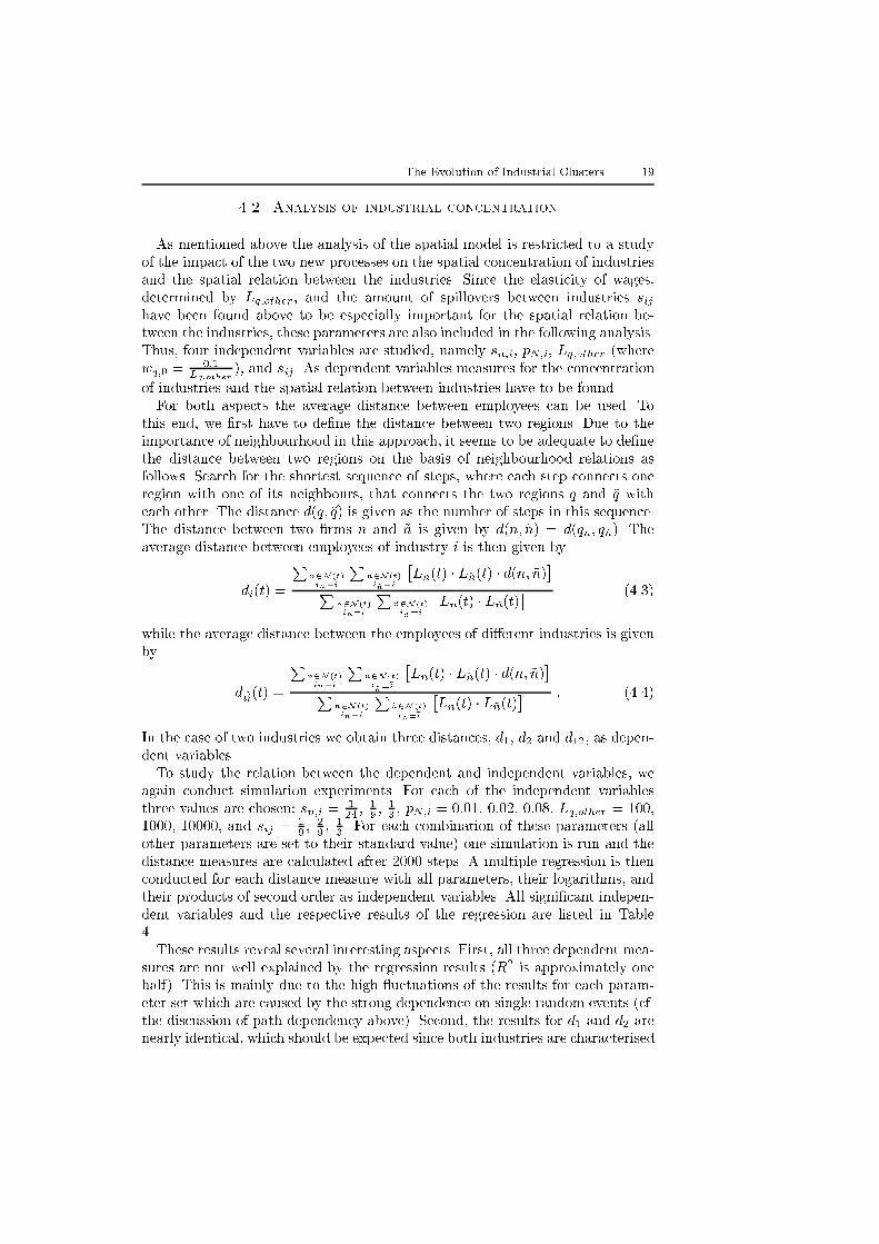
4.2. Analysis of industrial concentration
As mentioned above the analysis of the spatial model is restricted to a study
of the impact of the two new processes on the spatial concentration of industries
and the spatial relation between the industries. Since the elasticity of wages,
determined by Lq;other, and the amount of spillovers between industries sij
have been found above to be especially important for the spatial relation be-
tween the industries, these parameters are also included in the following analysis.
Thus, four independent variables are studied, namely sn;i, pN;i, Lq;other (where
wq;0 =0:1
Lq;other), and sij . As dependent variables measures for the concentration
of industries and the spatial relation between industries have to be found.
For both aspects the average distance between employees can be used. To
this end, we �rst have to de�ne the distance between two regions. Due to the
importance of neighbourhood in this approach, it seems to be adequate to de�ne
the distance between two regions on the basis of neighbourhood relations as
follows. Search for the shortest sequence of steps, where each step connects one
region with one of its neighbours, that connects the two regions q and ~q with
each other. The distance d(q; ~q) is given as the number of steps in this sequence.
The distance between two �rms n and ~n is given by d(n; ~n) = d(qn; q~n). The
average distance between employees of industry i is then given by
di(t) =
Pn2N(t)in=i
P~n2N(t)i~n=i
�Ln(t) � L~n(t) � d(n; ~n)
�P
n2N(t)
in=i
P~n2N(t)
i~n=i
�Ln(t) � L~n(t)
� (4.3)
while the average distance between the employees of di�erent industries is given
by
di~i(t) =
Pn2N(t)in=i
P~n2N(t)
i~n=~i
�Ln(t) � L~n(t) � d(n; ~n)
�P
n2N(t)
in=i
P~n2N(t)
i~n=~i
�Ln(t) � L~n(t)
� : (4.4)
In the case of two industries we obtain three distances, d1, d2 and d12, as depen-
dent variables.
To study the relation between the dependent and independent variables, we
again conduct simulation experiments. For each of the independent variables
three values are chosen: sn;i =124 ,
19 ,
13 , pN;i = 0:01, 0:02, 0:08, Lq;other = 100,
1000, 10000, and sij =19 ,
29 ,
13 . For each combination of these parameters (all
other parameters are set to their standard value) one simulation is run and the
distance measures are calculated after 2000 steps. A multiple regression is then
conducted for each distance measure with all parameters, their logarithms, and
their products of second order as independent variables. All signi�cant indepen-
dent variables and the respective results of the regression are listed in Table
4.
These results reveal several interesting aspects. First, all three dependent mea-
sures are not well explained by the regression results (R2 is approximately one
half). This is mainly due to the high uctuations of the results for each param-
eter set which are caused by the strong dependence on single random events (cf.
the discussion of path-dependency above). Second, the results for d1 and d2 are
nearly identical, which should be expected since both industries are characterised
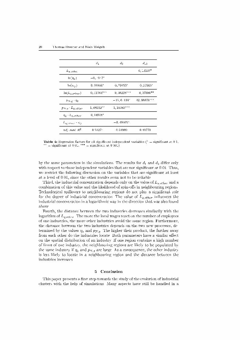
20 Thomas Brenner and Niels Weigelt
d1 d2 d12
Lq;other 0; 13135�
ln(�q) �0; 1947�
ln(sij) 0; 24406� 0; 29153� �0; 57965�
ln(Lq;other) �0; 41564��� �0; 36228��� �0; 37086��
pN;q � �q �15; 61138� 42; 98076���
pN;q � Lq;other 1; 08222�� 1; 10365���
�q � Lq;other 0; 18518�
Lq;other � sij �0; 49465�
adjusted R2 0.51274 0.54989 0.49773
Table 4: Regression factors for all signi�cant independent variables (� = signi�cant at 0.1,�� = signi�cant at 0.01, ��� = signi�cant at 0.001).
by the same parameters in the simulations. The results for d1 and d2 di�er only
with respect to those independent variables that are not signi�cant at 0.01. Thus,
we restrict the following discussion on the variables that are signi�cant at least
at a level of 0.01, since the other results seem not to be reliable.
Third, the industrial concentration depends only on the value of Lq;other and a
combination of this value and the likelihood of spin-o�s in neighbouring regions.
Technological spillovers to neighbouring regions do not play a signi�cant role
for the degree of industrial concentration. The value of Lq;other in uences the
industrial concentration in a logarithmic way in the direction that was also found
above.
Fourth, the distance between the two industries decreases similarily with the
logarithm of Lq;other. The more the local wages react on the number of employees
of one industries, the more other industries avoid the same region. Furthermore,
the distance between the two industries depends on the two new processes, de-
termined by the values �q and pN;q. The higher their product, the further away
from each other do the industries locate. Both parameters have a similar e�ect
on the spatial distribution of an industry. If one region contains a high number
of �rms of one industry, the neighbouring regions are likely to be populated by
the same industry if �q and pN;q are large. As a consequence, the other industry
is less likely to locate in a neighbouring region and the distance between the
industries increases.
5. Conclusion
This paper presents a �rst step towards the study of the evolution of industrial
clusters with the help of simulations. Many aspects have still be handled in a
The Evolution of Industrial Clusters 21
simplifying manner. Nevertheless, some insights have been obtained. First, it has
been found that the spatial structure locks in, independent of the parameters
chosen. Second, these lock-ins do in many cases not relate to the existence of
a stable spatial distribution of industrial activity. Instead, the dynamics show
a strong path-dependence which includes in many cases also the structure of
the spatial distribution. Third, the simulations reveal some circumstances that
should increase or decrease the degree of spatial concentration of an industry.
Nevertheless, this approach can and will be expanded with respect to several
aspects. First, in this approach no interactions between regions took place. A
more natural approach should be based on a two-dimensional cellular automa-
ton where neighbouring regions interact with each other. Second, the processes
within the regions should be modelled in more detail. Especially, the process of
innovation, the in uence of public research institutions, infrastructure, and pol-
itics, and the labour market are planned to be modelled in more detail. Finally,
the results of the simulations should be tested and compared with empirical data.
Some of this is planned to be done in further projects, some of it might be taken
up by other researchers.
References
Allen, P. M. (1997a). Cities and Regions as Evolutionary, Complex Systems. GeographicalSystems 4, 103{130.
Allen, P. M. (1997b). Cities and Regions as Self-Organizing Systems. Models of Complexity.Amsterdam: Gordon and Breach.
Audretsch, D. B. (1998). Agglomeration and the Location of Innovative Activity Oxford Reviewof Economic Policy 14, 18{29.
Becattini, G. (1990). The Marshallian Industrial District as a Socio-economic Notion. In: (Pyke,F., Becattini, G. and Sengenberger, W., Eds.) Industrial Districts and Inter-�rm Co-operation in Italy, pp. 37{51. Geneva: International Institute for Labour Studies.
Brenner, T. (2000). Industrial Clusters and Milieux: A Typology from an Evoluationary Per-spective. mimeo, Jena.
Camagni, R. P. (1995). The Concept of Innovative Milieu and Its Relevance for Public Policiesin European Lagging Regions. Papers in Regional Science 74, 317{340.
Camagni, R. P. & Diappi, L. (1991). A Supply-oriented Urban Dynamics Model with Innovationand Synergy E�ects. In: (Boyce, D. E., Nijkamp, P. and Shefer, D. ,Eds.) Regional Science,pp. 339{357. Berlin: Springer-Verlag.
Cani�els, M. C. J. and Verspagen, B. (1999). Spatial Distance in a Technology Gap Model .Working Paper 99.10, Eindhoven Centre for Innovation Studies.
Dalum, B. (1995). Local and Global Linkages: The Radiocommunications Cluster in NorthernDenmark . mimeo, Aalborg University.
Dei Ottati, G. (1994). Cooperation and Competition in the Industrial District as an Organi-sation Model European Planning Studies 2, 463{483.
Ellison, G. and Glaeser, E. L. (1994). Geographic Concentration in U.S. Manufacturing In-dusties: A Dartboard Approach. Working Paper No. 4840, National Bureau of EconomicResearch.
Ja�e, A.B., Trajtenberg, M. and Henderson, R. (1993). Geographic Localization of KnowledgeSpillovers as Evidenced by Patent Citations Quarterly Journal of Economics 79, 577{598.
Jonard, N. and Yildizoglu, M. (1998). Technological Diversity in an Evolutionary IndustryModel with Localized Learning and Network Externalities. Structural Change and Eco-nomic Dynamics 9, 35{53.
Krugman, P. (1991a). Geography and Trade. Cambridge: MIT Press.Krugman, P. (1991b). Increasing Returns and Economic Geography. Journal of Political Econ-
omy 99, 483{499.Lawson, C (1997). Territorial Clustering and High-Technology Innovation: From Industrial
Districts to Innovative Milieux . Working Paper No. 54, ESRC Centre for Business Re-search, University of Cambridge
Maillat, D. and Lecoq, B. (1992). New Technologies and Transformation of Regional Structuresin Europe: The Role of the Milieu. Entrepreneurship & Regional Development 4, 1{20.
22 Thomas Brenner and Niels Weigelt
Markusen, A. (1996). Sticky Places in Slippery Space: A Typology of Industrial Districts.Economic Geography 72, 293{313.
Matsuyama, K. and Takahashi, T. (1998). Self-Defeating Regional Concentration. Review ofEconomic Studies 65, 211{234.
Pyke, F. and Sengenberger, W., Eds (1992). Industrial Districts and Local Economic Regen-eration. Geneva: International Institute for Labour Studies.
Rabellotti, R. (1997). External Economies and Cooperation in Industrial Districts. Hound-mills: Macmillan Press Ltd.
Rosegrant, S. and Lampe, D. R. (1992). Route 128 . Basic Books.Saxenian, A.-L. (1994). Regional Advantage. Cambridge: Harvard University Press.Schweitzer, F. (1998). Modelling Migration and Economic Agglomeration with Active Brownian
Particles. adv. complex systems 1, 11{37.Scott, A. J. (1992). The Role of Large Producers in Industrial Districts: A Case Study of High
Technology Systems Houses in Southern California. Regional Studies 26, 265{275.van Dijk, M. P. (1995). Flexible Specialisation, The New Competition and Industrial Districts.
Small Business Economics 7, 15{27.Winer, B. J. (1971). Statistical Principles in Experimental Design. New York: McGraw-Hill.Witt, U. (1986). Firms' Market Behavior Under Imperfect Information and Economic Natural
Selection. Journal of Economic Behavior and Organization 7, 265-290.


