1 23 Natural Hazards Journal of the International Society for the Prevention and Mitigation of Natural Hazards ISSN 0921-030X Volume 58 Number 1 Nat Hazards (2011) 58:541-557 DOI 10.1007/ s11069-010-9685-4 Climate and solar signals in property damage losses from hurricanes affecting the United States Thomas H. Jagger, James B. Elsner & R. King Burch
Transcript
1 23
Natural HazardsJournal of the InternationalSociety for the Prevention andMitigation of Natural Hazards ISSN 0921-030XVolume 58Number 1 Nat Hazards (2011) 58:541-557DOI 10.1007/s11069-010-9685-4
Climate and solar signals in propertydamage losses from hurricanes affectingthe United States
Thomas H. Jagger, James B. Elsner &R. King Burch
1 23
Your article is protected by copyright and
all rights are held exclusively by Springer
Science+Business Media B.V.. This e-offprint
is for personal use only and shall not be self-
archived in electronic repositories. If you
wish to self-archive your work, please use the
accepted author’s version for posting to your
own website or your institution’s repository.
You may further deposit the accepted author’s
version on a funder’s repository at a funder’s
request, provided it is not made publicly
available until 12 months after publication.
ORI GIN AL PA PER
Climate and solar signals in property damage lossesfrom hurricanes affecting the United States
Thomas H. Jagger • James B. Elsner • R. King Burch
Received: 3 December 2008 / Accepted: 3 December 2010 / Published online: 30 December 2010� Springer Science+Business Media B.V. 2010
Abstract The authors show that historical property damage losses from US hurricanes
contain climate signals. The methodology is based on a statistical model that combines a
specification for the number of loss events with a specification for the amount of loss per
event. Separate models are developed for annual and extreme losses. A Markov chain
Monte Carlo procedure is used to generate posterior samples from the models. Results
indicate the chance of at least one loss event increases when the springtime north–south
surface pressure gradient over the North Atlantic is weaker than normal, the Atlantic ocean
is warmer than normal, El Nino is absent, and sunspots are few. However, given at least
one loss event, the magnitude of the loss per annum is related only to ocean temperature.
The 50-year return level for a loss event is largest under a scenario featuring a warm
Atlantic Ocean, a weak North Atlantic surface pressure gradient, El Nino, and few sun-
spots. The work provides a framework for anticipating hurricane losses on seasonal and
multi-year time scales.
Keywords Hurricanes � Property damage � Loss model � Environment � Risk compound
Poisson � MCMC
1 Introduction
Climatologists have constructed statistical models using climate variables to anticipate the
level of coastal hurricane activity (Elsner and Jagger 2006) and to account for changes in
hurricane intensity (Jagger and Elsner 2006; Elsner et al. 2008). Thus, we speculate that it
T. H. Jagger (&) � J. B. ElsnerDepartment of Geography, Florida State University, Tallahassee, FL 32306, USAe-mail: [email protected]
might be possible to detect climate signals in historical damage losses caused by hurri-
canes. The purpose of the present paper is to show evidence that specific climate and solar
signals are indeed detectable in records of damage losses from hurricanes along the US
coastline (Jagger et al. 2010).
Elucidating a connection between environmental conditions and economic threats from
natural hazards is an important new and interesting line of inquiry (Leckebusch et al.
2007). Although others have discovered climate signals in damage losses using bivariate
relationships including El Nino and wind shear (Katz 2002; Saunders and Lea 2005), this
paper is the first to look at the problem from a multivariate perspective. The work is based
on a recent study that uses pre-season environmental variables to anticipate insured losses
before the start of the hurricane season (Jagger et al. 2008). Here, we examine the mul-
tivariate relationship between a set of pre-determined environmental variables and damage
losses from hurricane winds.
Our loss modeling strategy is to combine separate models of event counts with event
losses. For modeling annual losses, we use a compound Poisson distribution with the
Poisson distribution on the annual number of loss events with a log-normal distribution for
each loss amount. The annual loss is therefore represented as a random sum of independent
losses, with variations in total loss decomposed into two sources, one attributable to
variations in the frequency of events and another to variations in loss from individual
events. For modeling extreme losses over longer time spans, we use an exceedance model
with a Poisson distribution for the annual number of losses exceeding a given threshold and
a generalized Pareto distribution (GPD) for the excess loss of each exceedance.
We begin in Sect. 2 by examining the normalized damage loss data. In Sect. 3 we
consider the environmental data associated with climate patterns and solar activity. In Sect.
4, we justify our decision to model small and large losses separately. In Sect. 5, we develop
a model for annual losses and in Sect. 6 we develop a model for extreme losses. Summary
and conclusions are provided in Sect. 7.
2 Damage losses from hurricanes
We obtain normalized damage loss data from the work of Pielke et al. (2008). The nor-
malization attempts to adjust loss amounts to what they would be if the hurricane struck in
the year 2005 by accounting for inflation and changes in wealth and population, plus an
additional factor to account for a change in the number of housing units that exceeds
population growth between the year of the loss and 2005. The methodology produces a
longitudinally consistent estimate of economic losses from past tropical cyclones affecting
the US Gulf and Atlantic coasts. A favorable assessment of the adjustment methodology
using two case studies is given in Changnon and Changnon (2009).
Economic damage loss is the direct loss associated with a hurricane’s impact. It does not
include losses due to business interruption or other macroeconomic effects including
demand surge and mitigation. Details and caveats for two slightly different normalization
procedures are provided in Pielke et al. (2008). Here we focus on the data set from the
Collins/Lowe methodology, but note that both data sets are quite similar. Results presented
in this study are not sensitive to the choice of data set as we demonstrate throughout.
We extend the data set in time by adding the estimated economic damage losses from
the three tropical cyclones during 2006 and 2007. The damage loss estimates are those
reported in the National Hurricane Center (NHC) storm summaries and derived by the
NHC by the American Insurance Services and the Property Claim Services. This is the
542 Nat Hazards (2011) 58:541–557
123
Author's personal copy
same primary data source used in the normalization methods described in Pielke et al.
(2008). There were six tropical cyclones that caused at least some damage in the United
States during this two-year period, but loss levels were quite small, especially when
compared with the losses experienced in 2004 and 2005. In fact loss levels for three of the
six tropical storms were below the $25 million reporting threshold (Alberto in 2006; Barry
and Gabrielle in 2007).
Tropical storm Ernesto in 2006 struck southern Florida and North Carolina. Total direct
damage losses are estimated at $500 mn (million). We estimate that 4/5ths of those losses
occurred in North Carolina where the storm was stronger at landfall. The total property
damage loss from tropical storm Erin is estimated at $35 mn and the total loss from
hurricane Humberto is estimated at $50 mn. Both Erin and Humberto hit the state of Texas.
The NHC suggests that Humberto’s damage total was low due to its small size and the fact
that it impacted a relatively unpopulated area. In addition, the large losses in the same area
from Hurricane Rita in 2005 may have moderated the amount of damage that could have
been done by Humberto. We make no attempt to normalize the losses from Ernesto, Erin,
and Humberto.
We keep separate the losses from a storm that makes multiple landfalls over different
regions. For example, in 1992 Hurricane Andrew produced a $52 bn (billion) loss in
southeast Florida and a separate $2 bn loss in Louisiana. When multiple landfall events are
included, the updated data set contains 221 loss events from 210 separate tropical cyclones
over the period 1900–2007. Figure 1 shows the distribution and time series of the damages
from all loss events. The histogram bars indicate the percentage of events with losses in
groups of $10 bn. The distribution is highly skewed with 88% of the events having losses
less than or equal to $10 bn and 95% of the events having losses less than $20 bn.
The greatest loss occurred with the 1926 hurricane that struck southeast Florida creating
an estimated damage loss adjusted to 2005 dollars of $129 bn. The Galveston hurricane of
1900 ranks second with an estimated loss of $99 bn, and hurricane Katrina of 2005 ranks
third with an estimated total loss of $81 bn. Years with more than one loss have more than
one point on the plot. There is large year-to-year variability but no obvious long-term
trend, although here the data are not disaggregated into loss amount and the number of loss
events.
1900 1920 1940 1960 1980 2000
0
20
40
60
80
100
120
140
Year
Loss
Dam
age
[200
5 $U
S b
n]
a
Loss Damage [2005 $US bn]
Fre
quen
cy
0 40 80 120
0
50
100
150
200b
Fig. 1 Hurricane damage losses. a Time series plot of per storm damage losses from hurricanes in theUnited States (excluding Hawaii). Some years have more than one loss event. The number of loss events isincreasing over time. b The distribution of per storm damage losses. The actual values are located as red ticmarks above the abscissa. The loss distribution is positively skewed with relatively few events generatingmost of the damage losses
Nat Hazards (2011) 58:541–557 543
123
Author's personal copy
The damage loss exceedances are shown in Table 1. Of the 221 loss events from 1900
to 2007, 169 exceeded $100 mn in losses and 28 of these exceeded $10 bn. The two events
producing losses less than $1 mn include Gustav in 2002 and Dean in 1995. The distri-
bution of losses is similar in the Collins/Lowe (CL) data and the Pielke/Landsea (PL) data,
although the Collins/Lowe data has somewhat larger losses. The CL method differs from
the PL method by including a normalization factor for changes in the number of housing
units exceeding population growth.
Another way to examine the data is to look at cumulative losses by hurricane intensity.
Table 2 shows losses in billions of US dollars from 1900–2007, inclusive by intensity
categories. Category 0 is the minimum tropical storm threshold of 17 m s-1, and category
1 is the minimum hurricane threshold of 33 m s-1. From this table, we can see that
cyclones of tropical storm intensity or higher accounted for of $1,103.9 bn 2005 adjusted
$US while cyclones of hurricane intensity or higher accounted for $1,063.1 bn. Here again
we see the similarity in the two data sets and that category 4 and 5’s, although rare, have
historically accounted for nearly 50% of all damage losses.
Figure 2 shows the annual number of loss events and their distribution. There are five
years with 6 loss events, with the most recent being 2005. The annual rate of loss events is
1.94 per year with a variance of 2.48 (events/year)2. There is a distinct upward trend in the
number of loss events attributable to some extent to an increase in coastal population. As
population increases so do the number of loss events from the weaker tropical cyclones.
Indeed, prior to 1950 the number of loss events from tropical storms was 6% of the total
number of events. This increases to nearly 38% from 1950 onward. It is noted that although
the per storm damage losses have been adjusted for increases in coastal population, the
number of loss events have not. An early tropical cyclone making landfall in an area void
of a built environment did not generate losses, so there is nothing to adjust. Additional
Table 1 Damage loss exceedances ($US adjusted to 2005)
Exceedance $US (2005) Number of events (CL) Number of events (PL)
1 Million 219 219
10 Million 207 207
100 Million 169 169
1 Billion 98 94
10 Billion 28 27
100 Billion 1 1
Values are the number of events exceeding various loss thresholds. Data from 1900–2007, inclusive
CL is for the Collins and Lowe data set and PL is for the Pielke and Landsea data set
Table 2 Cumulative losses bySaffir-Simpson hurricane inten-sity category in billions of $USadjusted to 2005
Data from 1900–2007, inclusive
CL is for the Collins and Lowedata set and PL is for the Pielkeand Landsea data set
Category(Saffir/Simpson)
Cumulativelosses (CL)
Cumulativelosses (PL)
0 1,103.9 1,125.1
1 1,063.1 1,084.5
2 1,022.7 1,045.6
3 941.4 964.4
4 533.1 557.3
5 79.4 79.3
544 Nat Hazards (2011) 58:541–557
123
Author's personal copy
descriptive characteristics of severe Atlantic hurricanes in the United States are provided in
Changnon (2009).
In this study, we primarily focus on the largest losses from the set of strongest tropical
cyclones. There is positive skewness in per storm loss amounts, so we transform them
using logarithms. We use base 10 logarithms, so a billion dollar loss has a value of 9
making it is easy to mentally convert back to actual losses.
3 Climate and solar variables
Statistical relationships between US hurricane activity and climate are well established
(Elsner et al. 2004; Murnane et al. 2000). More importantly for the present work, recent
studies have modeled the wind speeds of hurricanes at or near landfall (Jagger et al. 2001;
Jagger and Elsner 2006). Results show exceedance probabilities of strong hurricanes vary
appreciably with the El Nino cycle (ENSO), the North Atlantic Oscillation (NAO), and
sea-surface temperature (SST). Recent work also shows a linkage between US hurricane
activity and sunspot numbers (SSN) (Elsner and Jagger 2008; Elsner et al. 2010).
The ENSO is characterized by basin-scale fluctuations in sea-level pressure between
Tahiti and Darwin. Although noisier than equatorial Pacific ocean temperatures, pressure
values are available back to 1900. The Southern Oscillation Index (SOI) is defined as the
normalized sea-level pressure difference between Tahiti and Darwin (in units of standard
deviation). Negative values of the SOI indicate an El Nino event. The relationship between
ENSO and hurricane activity is strongest during the hurricane season, so we use a
1900 1920 1940 1960 1980 2000
0
1
2
3
4
5
6
Year
Num
ber
of L
oss
Eve
nts a
0 1 2 3 4 5 6
Number of Loss Events
Fre
quen
cy
0
5
10
15
20
25
30
35b
1900 1920 1940 1960 1980 2000
8
9
10
11
Year
Log
Loss
[200
5 $U
S] c
Log Loss [2005 $US]
Fre
quen
cy6 7 8 9 10 11 12
0
5
10
15
20d
Fig. 2 Number of loss events and the amount of loss per event (normalized to 2005 dollars). a Time seriesand b distribution of the number of loss events. The number of loss events is increasing over the time period.c Time series and d distribution of the amount of damage losses. The amount of losses is on a logarithmic(base 10) scale. There is no trend over time in the amount of normalized losses
Nat Hazards (2011) 58:541–557 545
123
Author's personal copy
August–October average of the SOI as a climate factor. The monthly SOI values (Rope-
lewski and Jones 1987) are obtained from the Climatic Research Unit (CRU).
The NAO is characterized by fluctuations in sea level pressure (SLP) differences. Index
values for the NAO (NAOI) are calculated as the difference in SLP between Gibraltar and
a station over southwest Iceland (in units of standard deviation), and are obtained from the
CRU (Jones et al. 1997). The values are averaged over the pre- and early-hurricane season
months of May and June (Elsner et al. 2001) as this is when the relationship with hurricane
activity is strongest (Elsner and Jagger 2006).
SST values are a blend of modeled and observed data. Raw (unsmoothed and not
detrended) monthly values dating back to 1871 (in units of �C) over the North Atlantic
basin (0 to 70�N) are obtained from the NOAA-CIRES Climate Diagnostics Center. For
this study, we average the SST values over the peak hurricane season months of August
through October.
For SSN, we use the monthly total sunspot number for September (the peak month of
the hurricane season). Sunspots are magnetic disturbances of the sun surface having both
dark and brighter regions. The brighter regions (plages and faculae) increase the intensity
of the ultraviolet emissions. Increased sunspot numbers correspond to more magnetic
disturbances. Sunspot numbers produced by the Solar Influences Data Analysis Center(SIDC), World Data Center for the Sunspot Index, at the Royal Observatory of Belgium are
obtained from the US National Oceanic and Atmospheric Administration.
In summary, normalized historical damage losses from hurricane events over the period
1900–2007 will be modeled using the above climate and solar data. These covariates are
chosen based on previous studies relating climate factors to the variability in US hurricane
activity. We make no attempt to search for new covariates.
Time series’ of the covariates are plotted in Fig. 3. The SOI and NAO variables have no
obvious long-term trend. The SST variable, on the other hand, indicates warming from
1900 to about 1940 followed by cooling until about 1980 then warming since. This pattern
has been called the Atlantic multidecadal oscillation. The SSN variable shows an obvious
11-year cycle and increasing amplitude of the cycle through 1960 with a declining
amplitude since.
Upper and lower quartile values of the SOI are 0.40 and -0.90 SD, respectively with a
median (mean) value of -0.18 (-0.16) SD. Years of above (below) normal SOI corre-
spond to La Nina (El Nino) events and thus a higher probability of at least one US
hurricane. The upper and lower quartile values of the NAO are 0.40 and -1.09 SD,
respectively with a median (mean) value of -0.39 (-0.33) SD. Years of below (above)
normal values of the NAO correspond to a weak (strong) NAO phase and thus to higher
(lower) probability of US hurricanes. The upper and lower quartile values of the Atlantic
SST anomalies are 0.22 and �0:16�C, respectively. Years of above (below) normal values
of SST correspond to higher (lower) probability of hurricane activity. The upper and lower
quartile values of the September SSN are 91.7 and 17.1, respectively with a median (mean)
value of 50.2 (62.0). Years of below (above) normal SSN correspond to a lower (higher)
probability of US hurricanes. The largest correlation among the covariates occurs between
SSN and SST at a value of ?0.18.
As an initial look at losses relative to variations in the covariates, here we compare
conditional distributions of per storm damage losses. Table 3 lists the damage amounts at
the median and upper 99th percentile value for the damage loss data sets and the damage
ratio as the amount of damage during above normal years to the amount during below
normal years. It can be seen that during seasons characterized by La Nina conditions
(above normal values of SOI), the median losses are greater by a factor of more than two
546 Nat Hazards (2011) 58:541–557
123
Author's personal copy
compared with years with El Nino conditions. However, extreme losses are higher during
years featuring El Nino conditions. During seasons with below normal springtime NAO
conditions, the damages tend to be greater at the median level and even more so at the
extremes.
1900 1920 1940 1960 1980 2000
−2
−1
0
1
2
Year
SO
I [s.
d.]
a
1900 1920 1940 1960 1980 2000
−2
−1
0
1
2
3
Year
NA
O [s
.d.]
b
1900 1920 1940 1960 1980 2000
−0.4
−0.2
0.0
0.2
0.4
0.6
Year
SS
T [°
C]
c
1900 1920 1940 1960 1980 2000
0
50
100
150
200
Year
SS
N [c
ount
]
d
Fig. 3 Time series of the four variables (covariates) used to model damage losses from hurricanes. Thevariables include the Southern Oscillation Index (SOI), an index of the North Atlantic Oscillation (NAO),North Atlantic sea-surface temperature (SST) and sunspot number (SSN). A description of the variables isgiven in the text
Table 3 Loss amounts from hurricanes in billions of $ US adjusted to 2005 along with conditional damageratios
Quantile CL PL
50% 99% 50% 99%
Damage 0.544 79.377 0.530 79.830
SOI 2.340 0.588 2.257 0.580
NAO 0.845 0.363 0.868 0.320
SST 0.437 1.271 0.477 1.211
SSN 0.282 0.437 0.309 0.430
The damage loss ratio is the respective quantile amount of loss per storm during above normal years to theamount during below normal years independently for each covariate
CL is for the Collins and Lowe data set and PL is for the Pielke and Landsea data set
Nat Hazards (2011) 58:541–557 547
123
Author's personal copy
Seasons characterized by higher than average SST show smaller loss amounts at the
median levels compared with seasons characterized by lower SST. There is, however, a
modest increase in loss amounts during warm years over loss amounts during the cold
years at the upper tails of the distribution. During seasons with below normal sunspots,
damage losses tend to be greater at the median level and similarly so at the extremes. These
results are expected from what we know about how these environmental factors influence
US hurricane activity (Elsner and Jagger 2006; Jagger and Elsner 2006). We note that the
CL and PL loss data sets give nearly the same results.
4 Large and small losses
Figure 4 shows distributions of losses by the Saffir-Simpson category of storm intensity.
The logarithm of the losses by category are plotted as red horizontal tick marks. The
median loss in each category is shown by a black horizontal line. The distribution is shown
by the gray area. Wider areas correspond to more frequent loss events at that amount of
loss. The distributions tend to be fairly symmetric on the log scale.
The range of damage losses tends to be greater for the lower category storms. For
instance, at the 80% interval of losses the range is from 6.8 to 9.0 for category 0 storms,
and from 7.2 to 9.1 for category 1 storms, this is about 2.2 and 1.9, respectively, or
approximately a factor of 100. In comparison, the category 2, 3, 4, and 5 ranges are 1.3,
1.5, 1.4, and 1.1, respectively. Thus it makes sense to model tropical storms (category 0)
and category 1 hurricanes separately from category 2 and higher storms. However, there is
a practical limitation in that we lose 109 of the 212 storms. Thus, for this paper, we restrict
our analysis to category 1 and higher tropical cyclones (hurricanes only) as a compromise
between removing too much data and keeping too many small loss events.
The total damage from the 221 events (1900–2007) calibrated to 2005 is estimated at
US $1.1 trillion. It is often noted that 80% of the total damage from tropical cyclones is
caused by 20% of the biggest loss events. Figure 5 shows that the distribution of damage
data is more skewed than that. In fact, the top 35 loss events (less than 16% of the total
number of loss events) account for more than 81% of the total loss amount.
The relative infrequency of the largest loss events argues for a split that favors more
data for modeling the largest losses. Here, we use a threshold of one billion $US and find
that 90 of the 160 hurricane events (56.3%) exceed this value. The remaining 70 events
4
6
8
10
12
0 1 2 3 4 5
Saffir−Simpson Category
Log
Loss
[200
5 $U
S]
61 48 38 56 15 3
Fig. 4 Damage losses by Saffir-Simpson hurricane category. Theactual losses are given ashorizontal red ticks. The medianloss in each category is shown bya black horizontal line. Thesmoothed distribution is shownwith a gray area. Wider regionscorrespond to more frequent lossevents at that amount of loss.Category 0 refers to tropicalcyclones of tropical stormintensity
548 Nat Hazards (2011) 58:541–557
123
Author's personal copy
(43.7%) account for only 15.4% of the total damages. Thus, it is reasonable to assume that
small loss events are below the ‘‘noise’’ level. In summary, our focus here is on the set of
large losses from the stronger tropical cyclones. Note also that here we do not examine the
geographic variation of losses as was done for the state of Florida in Malmstadt et al.
(2009).
5 Annual loss model
Given a loss event, the logarithm of the loss amount is modeled as a truncated normal
distribution. The only statistically significant climate signal in the loss amount is the SST.
We model this signal by regressing the location parameter of the truncated normal dis-
tribution onto SST for large losses. Thus given a loss event, the magnitude of the loss
increases with increasing ocean warmth. This is consistent with SST acting as a proxy for
upper-ocean heat, a source of energy for hurricanes (Emanuel 1991).
To arrive at an estimate of the annual loss, we need to combine this loss amount
estimate given an event with the frequency of loss events. Since we divide loss events into
large and small events, we use two models. Thus, given a mean annual rate of large (small)
loss events, the annual number of large (small) loss events follows a Poisson distribution
with the natural logarithm of the loss event rate given as a linear function of the climate
variables. We find that SST, NAO, SOI, and SSN are all statistically significant indicators
of the frequency of large losses, but none of the climate variables are important for the
frequency of small losses.
Mathematically we write the model for large losses as:
A ¼ 10L
L�Normalðl; r2ÞT½9;1�l ¼ a0 þ a1SST
N �PoissonðkÞk ¼ expðb0 þ b1SSTþ b2NAOþ b3SOIþ b4SSNÞ
ð1Þ
where A is the loss amount for an event, N is the yearly event count and k is the yearly loss
frequency. The symbol * refers to a stochastic relationship and indicates that the variable
on the left-hand side is a random draw (sample) from a distribution specified on the
5 6 7 8 9 10 11
0.0
0.2
0.4
0.6
0.8
1.0
Log Loss [2005 $US]
Cum
ulat
ive
Dis
trib
utio
n
Fig. 5 Cumulative distributionof per storm damage loss. Thevalues on the ordinate are thefraction of damage losses lessthan or equal to the damagelosses on the abscissa. Losses areconverted to a logarithmic (base10) scale. The horizontal dottedline is the 80th percentile and thevertical dotted line is the lossamount of the 20th largest lossevent. The actual values arelocated as red tic marks above theabscissa
Nat Hazards (2011) 58:541–557 549
123
Author's personal copy
right-hand side. The equal sign indicates a logical relationship with the variable on the left-
hand side algebraically related to variables on the right-hand side. As mentioned, the size
of the loss is modeled as a truncated normal distribution with parameters l and r2 indi-
cating the location and scale for the distribution and T[9,?] indicating the truncation
limits. Unlike the normal distribution, the location and scale parameters of the truncated
normal distribution are not the same as its mean and variance. In short, the model describes
a compound Poisson process with rate k and logarithm of the loss amount distributed as a
truncated normal distribution with parameters l and r.
The chi-square goodness-of-fit statistic indicates the rate model is adequate. Further-
more, there is no trend in the deviance residuals implying the rate model for large losses
conditioned on the environmental variables chosen is statistically stationary and the
addition of a trend term does not improve the model. This suggests to us that there is no
significant historical under reporting of the number of loss events from hurricanes in the
United States over the period considered here. Note this is not likely the case for losses
from weaker tropical storms.
The final model that combines the frequency of loss events with the magnitude of the
loss given an event uses a hierarchical Bayesian specification. Bayesian models provide
posterior distributions of model parameters, as opposed to a frequentist model using
maximum likelihood estimation (MLE) which only provides the parameter estimate and
prediction error. For non-normal distributions, these MLEs lead to biased predictions. Here
we chose flat (non-informative) priors for the location and precision (1/r2) parameters to
minimize their influence on the posterior distributions.
The final model is selected from a set of possible models by comparing the Deviance
Information Criterion (DIC) for each model and then choosing the model with the smallest
DIC. The DIC is used for selecting among candidate models within a Bayesian framework
in the same way that AIC is used for selecting among candidate models within a maximum
likelihood framework (Spiegelhalter et al. 2002). DIC is particularly useful when the
posterior distributions of the models are obtained by Markov Chain Monte Carlo (MCMC)
simulation. The model with the smallest DIC is taken as the one that would best predict a
replicate data set having the same statistics as the observed data set.
Given the hierarchical form of the model, samples of the annual losses are generated
using WinBUGS (Windows version of Bayesian inference Using Gibbs Sampling)
developed at the Medical Research Council in the UK (Gilks et al. 1998; Spiegelhalter
et al. 1996). WinBUGS chooses an appropriate MCMC sampling algorithm based on the
model structure. In this way, annual losses are sampled conditional on the model coeffi-
cients and the observed values of the covariates. The cost associated with a Bayesian
approach is the requirement to formally specify prior beliefs. As mentioned, here we take
the standard route and assume non-informative priors.
MCMC, in particular Gibbs sampling, is used to sample the parameters given the data
since no closed form solution exists for the posterior distribution of the model parameters
in the truncated normal (or for the generalized Pareto distribution (GPD) used in the next
section). Indeed, WinBUGS is useful in that it allows us to sample the parameters from the
posteriors created from arbitrary likelihood functions. As far as we are aware, there is no
software for finding the maximum likelihood estimates of the regression parameters for a
truncated normal distribution.
We check for mixing and convergence by examining successive samples of the
parameters. Samples from the posterior distributions of the parameters indicate relatively
good mixing and quick settling, as two different sets of initial conditions produce sample
values that fluctuate around a fixed mean. Based on these diagnostics, we discard the first
550 Nat Hazards (2011) 58:541–557
123
Author's personal copy
10,000 samples and analyze the output from the next 10,000 samples. The utility of the
Bayesian approach for modeling the mean number of coastal hurricanes is described in
Elsner and Jagger (2004) and for predicting damage losses is described in Jagger et al.
(2008).
Figure 6 shows the posterior predictive distributions of annually aggregated losses for
six different climate scenarios. The set of scenarios is ordered by increasingly favorable
conditions for hurricanes in the United States from upper left to lower right. Each panel
shows the probability of no losses during the year (red bar) and the probability of losses
given at least one loss event (black histogram). The upper-left panel shows the posterior
probabilities for a year during which the SST is much below normal, the NAO is much
above normal, there is a strong El Nino in the Pacific, and the sun is active (many spots).
The specific covariate values are listed in the figure caption.
The results show a relatively large probability of no loss events (37%) under this
scenario. The estimated annual loss taking into account the non-zero probability of no loss
events is centered in the range between $0.1 and $1 bn. As the climate factors change to
indicate more favorable conditions for hurricanes, the posterior predictive distribution of
annual losses become more ominous. The probability of no losses decreases to less than
Log Loss [2005 $US]
Pro
babi
lity
10 150.00.10.20.30.40.50.6
a
Log Loss [2005 $US]
Pro
babi
lity
10 150.00.10.20.30.40.50.6
b
Log Loss [2005 $US]
Pro
babi
lity
10 150.00.10.20.30.40.50.6
c
Log Loss [2005 $US]P
roba
bilit
y10 15
0.00.10.20.30.40.50.6
d
Log Loss [2005 $US]
Pro
babi
lity
10 150.00.10.20.30.40.50.6
e
Log Loss [2005 $US]
Pro
babi
lity
0 5 0 5
0 5 0 5
0 5 0 5 10 150.00.10.20.30.40.50.6
f
Fig. 6 Modeled annual losses for six different climate scenarios. Each panel is a different scenario with thered bar indicating the probability of no loss event for that year and the black histogram bars indicating theposterior predictive distribution of the amount of losses. The panels are ordered from upper left to lowerright by conditions increasingly favorable for US hurricanes. a SST ¼ �0:52�C; NAO ¼ þ2:9 SD, SOI ¼�2:3 SD, and SSN = 236, b SST ¼ �0:24�C; NAO ¼ þ0:7 SD, SOI ¼ �1:1 SD, and SSN = 115,c SST ¼ þ0:01�C; NAO ¼ �0:3 SD, SOI ¼ �0:2 SD, and SSN = 62, d SST ¼ þ0:27�C; NAO ¼ �1:4SD, SOI ¼ þ0:8 SD, and SSN = 9, e SST ¼ þ0:43�C; NAO ¼ �1:3 SD, SOI ¼ �0:1 SD, and SSN = 5,and f SST ¼ þ0:61�C; NAO ¼ �2:7 SD, SOI ¼ þ2:6 SD, and SSN = 1
Nat Hazards (2011) 58:541–557 551
123
Author's personal copy
1% and the expected annual total loss amount exceeding $100 billion in the most favorable
scenario considered (lower-right panel). Keep in mind that all damage loss amounts are
converted to 2005 US dollars. Results from the model are remarkable in showing distinct
climate signals in property damage losses in the United States from hurricanes. In general,
the annual expected loss increases with warmer Atlantic SSTs, La Nina conditions, a
negative phase of the NAO, and fewer sunspots.
6 Extreme loss model
While the above model estimates the distribution of annual losses associated with varia-
tions in environmental conditions, for financial planning it might be more important to
estimate the distribution of extreme losses and the probable maximum loss. In this case, the
normal distribution is replaced by the Generalized Pareto Distribution (GPD) for the
common logarithm of the loss amount, L = log10(A). In what follows the term loss refers
to the transformed loss amounts on the common logarithmic scale.
Consider observations from a collection of random variables in which only those
observations that exceed a fixed value are kept. As the magnitude of this value increases,
the GPD family represents the limiting behavior of each new collection of random vari-
ables if the limit exists. This property makes the family of GPD a good choice for modeling
extreme events including large losses from hurricanes. The choice of threshold, above
which we treat the values as extreme, is a compromise between retaining enough obser-
vations to properly estimate the distributional parameters (scale and shape), but few
enough that the observations follow a GPD.
The GPD describes the distribution of losses that exceed a threshold l but not the
frequency of losses exceeding that threshold. As we did with the annual loss model, we
specify that, given a rate of loss events above the threshold, the number of loss events
follows a Poisson distribution. Here there is no need to separate out small loss events as we
are only interested in the large ones. Combining the GPD for large losses with the Poisson
distribution for the frequency of loss events above the threshold allows us to obtain return
periods for given levels (amounts) of loss.
We model the exceedances, L - l, as samples from a family of GPDs so that for any
threshold l, and any event with the loss L, the probability that L exceeds some arbitrary
level x above l is
PrðL [ xþ ljL [ lÞ ¼expð� x
rÞ n ¼ 0
1þ nrl
x� ��1
nn 6¼ 0
8<: ð2Þ
¼ GPDðxjrl; nÞ ð3Þ
where rl [ 0; x� 0, and rl þ nx� 0. If the exceedances above l0 follow a GPD then the
exceedances above l [ l0 follow a GPD with the same shape, n and scale that shifts linearly
with the threshold:
rl ¼ r0 þ nl
The parameters rl and n are the scale and shape parameters respectively. If n� 0 the
maximum loss using the GPD model is unbounded but for n\ 0 the GPD has an upper
limit of Lmax ¼ lþ rl=jnj so the maximum probable loss amount is bounded by $ 10Lmax .
The equation for rl specifies that if the values follow a GPD, then for any threshold the
552 Nat Hazards (2011) 58:541–557
123
Author's personal copy
distribution of exceedances is GPD with the same value of the shape parameter (n) from
the original distribution and a scale parameter that changes linearly with the threshold at a
rate equal to the shape parameter.
We determine the threshold value for the set of losses at 9 i.e. a loss amount of $1 bn US
by examining the mean residual life plot (not shown). This is a plot of the mean value of
the exceedances as a function of the threshold. If the data follow a GPD, this plot is linear.
The threshold is chosen as the smallest value where the function is linear for all larger
thresholds (see Coles 2001, Chap. 4).
The GPD describes the distribution losses for each hurricane whose losses exceed l, but
not the number of loss events exceeding l. Instead we assume that the number of loss
events in year y that exceed l has a Poisson distribution with mean (or exceedance) rate is
kl. Thus, by combining the exceedance probability and the exceedance rate with our
assumption that they are independent, we get a Poisson distribution for the number of loss
events per year with losses exceeding m (Nm) with a rate given by
km ¼ kl PrðL [ mjL [ lÞ: ð4Þ
This specification is physically realistic, since it allows us to model loss occurrence sep-
arately from loss amount. Moreover from a practical perspective, rather than a return rate
per loss occurrence, the above specification allows us to obtain an annual return rate on the
extreme losses, which is more meaningful for the business of risk and insurance.
Now, the probability that the yearly maximum loss will be less than m is the probability
that Nm = 0. Since Nm has a Poisson distribution
PrðLmax�mÞ ¼ PrðNm ¼ 0Þ ð5Þ
¼ expð�kmÞ ð6Þ
¼ exp �klGPDðm� ljrl; nÞf g ð7ÞIf we make the substitution for n = 0:
r ¼ knl rl ð8Þ
l ¼ lþ r� rl
nð9Þ
then
PrðLmax�mÞ ¼ exp � 1þ nm� l
r
� �h i�1n
� �ð10Þ
has a Generalized Extreme Value (GEV) distribution, which is in canonical form. If n = 0
then we make the substitutions
r ¼ rl
l ¼ lþ r logðklÞ
then
PrðLmax�mÞ ¼ exp � exp � m� lr
� �h in o: ð11Þ
We convert the peaks-over-threshold parameters kl; rl; n to the canonical GEV
parameters l, r, n, to compare results obtained with different thresholds and calculate
return levels. Using the canonical GEV parameters, the yearly (seasonal) return level, rl(r),
Nat Hazards (2011) 58:541–557 553
123
Author's personal copy
corresponding to a given return period, r is calculated by solving for m in PrðLmax�mÞ ¼ 1r
giving
rlðrÞ ¼ lþ rn log r
r�1
� ��n�1h in o
n 6¼ 0
l� r � log log rr�1
� �� n ¼ 0:
ð12Þ
Additional details are given in Coles (2001, Chap. 4).
This model of extreme losses also uses a Bayesian specification, and a MCMC method
is used to sample from the posterior predictive distributions. Here, we are interested in the
return level as a function of return period. The return level is determined by the magnitude
of individual extreme loss events and the frequency of such events above a threshold rate.
The number of extreme loss events over a specified period is modeled using a Poisson
distribution with the natural logarithm of the rate specified as a linear function of the four
covariates. The losses minus the threshold L - l is modeled using a GPD where the
logarithm of the scale parameter and the shape parameter are both linear functions of the
four covariates.
As before, samples of the return levels are generated using WinBUGS with non-
informative prior distributions. Samples from the posterior distribution of the model
parameters indicate good mixing and good convergence properties. We discard the first
10,000 samples and analyze the output from the next 10,000 samples. Applications of
Bayesian extremal analysis are found in Coles and Tawn (1996), Walshaw (2000), Katz
et al. (2002), Coles et al. (2003), Hsieh (2004), and Jagger and Elsner (2006).
For a given sample of the GEV parameters Eq. 12 is used to calculate a posterior sample
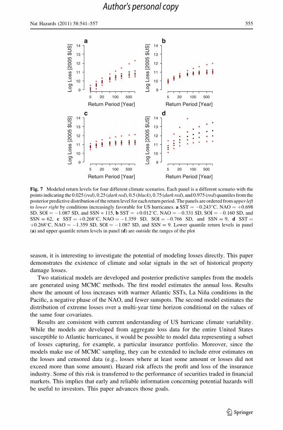
of the return levels associated with each return period of interest. Figure 7 shows the
posterior predictive distributions of return levels of individual loss events for four different
climate scenarios using quantile values. For each return period, the 0.025, 0.25, 0.5, 0.75,
and 0.975 quantile values of the return levels are plotted. The first scenario is characterized
by covariates in favor of fewer hurricanes, the second scenario represents long-term cli-
matological conditions, the third scenario is characterized by covariates favoring more
hurricanes, and the fourth scenario is characterized by covariates favoring stronger hur-
ricanes. The loss distribution changes substantially depending on the climate scenario and
the directions of change are consistent with our understanding about the relationship
between climate variability and hurricane activity.
Under the first scenario, we find the median return level of a 50-year extreme event at
approximately $18 bn; this compares with a median return level of the same 50-year
extreme event loss of approximately $793 bn under the fourth scenario. Thus, the model
can be useful for projecting extreme losses over time horizons longer than a year given
values of the covariates. Note that the results are interpreted as the posterior distributions
of the return level for a return period of 50 years with the covariate values as extreme or
more extreme than 1 standard deviation. With 4 independent covariates and an annual
probability of about 16% that a particular covariate is more than 1 SD. from its mean, the
chance that all covariates will be this extreme or more in a given year is less than 0.1%.
7 Summary and conclusions
Hurricanes are capable of generating large financial losses. Annual loss totals are directly
related to the intensity and frequency of hurricanes affecting the coast. Since a detectable
amount of skill exists in forecasting coastal hurricane activity months in advance of the
554 Nat Hazards (2011) 58:541–557
123
Author's personal copy
season, it is interesting to investigate the potential of modeling losses directly. This paper
demonstrates the existence of climate and solar signals in the set of historical property
damage losses.
Two statistical models are developed and posterior predictive samples from the models
are generated using MCMC methods. The first model estimates the annual loss. Results
show the amount of loss increases with warmer Atlantic SSTs, La Nina conditions in the
Pacific, a negative phase of the NAO, and fewer sunspots. The second model estimates the
distribution of extreme losses over a multi-year time horizon conditional on the values of
the same four covariates.
Results are consistent with current understanding of US hurricane climate variability.
While the models are developed from aggregate loss data for the entire United States
susceptible to Atlantic hurricanes, it would be possible to model data representing a subset
of losses capturing, for example, a particular insurance portfolio. Moreover, since the
models make use of MCMC sampling, they can be extended to include error estimates on
the losses and censored data (e.g., losses where at least some amount or losses did not
exceed more than some amount). Hazard risk affects the profit and loss of the insurance
industry. Some of this risk is transferred to the performance of securities traded in financial
markets. This implies that early and reliable information concerning potential hazards will
be useful to investors. This paper advances those goals.
100 500
9
10
11
12
13
14
Return Period [Year]
Log
Loss
[200
5 $U
S] a
100 500
9
10
11
12
13
14
Return Period [Year]
Log
Loss
[200
5 $U
S] b
100 500
9
10
11
12
13
14
Return Period [Year]
Log
Loss
[200
5 $U
S] c
5 20 5 20
5 20 5 20 100 500
9
10
11
12
13
14
Return Period [Year]
Log
Loss
[200
5 $U
S] d
Fig. 7 Modeled return levels for four different climate scenarios. Each panel is a different scenario with thepoints indicating the 0.025 (red), 0.25 (dark red), 0.5 (black), 0.75 (dark red), and 0.975 (red) quantiles from theposterior predictive distribution of the return level for each return period. The panels are ordered from upper leftto lower right by conditions increasingly favorable for US hurricanes. a SST ¼ �0:243�C; NAO ¼ þ0:698SD, SOI ¼ �1:087 SD, and SSN = 115, b SST ¼ þ0:012�C; NAO ¼ �0:331 SD, SOI ¼ �0:160 SD, andSSN = 62, c SST ¼ þ0:268�C; NAO ¼ �1:359 SD, SOI ¼ �0:766 SD, and SSN = 9, d SST ¼þ0:268�C; NAO ¼ �1:359 SD, SOI ¼ �1:087 SD, and SSN = 9. Lower quantile return levels in panel(a) and upper quantile return levels in panel (d) are outside the ranges of the plot
Nat Hazards (2011) 58:541–557 555
123
Author's personal copy
The study is limited by the historical loss data. As noted above, although the per storm
damage losses have been adjusted for increases in coastal population, the number of loss
events have not. An early tropical cyclone making landfall in an area void of a built
environment did not generate losses, so there is nothing to adjust. This can be rectified
using a model (e.g., HAZUS) that can estimate losses from historical hurricanes using
constant building exposure data.
Traditional hurricane risk models used by the insurance industry rely on a catalog of
storms that represent the historical data in some way or another. While useful for esti-
mating expected annual loss and loss exceedance levels for portfolio losses, these catalogs
are not easily suited for anticipating losses based on a variable climate. Specifically, at the
core of the catalog is a very large set of synthetic storms (more than 50,000) and a way to
assign a probability to each. To condition the synthetic storms on several climate variables
would require a catalog size that is at least an order of magnitude larger. The approach
demonstrated here provides an alternative way to anticipate losses on the seasonal and
multi-year time scales that avoids the problem of excessively large catalogs.
Concerning the future, increases in ocean temperature will raise a hurricane’s potential
intensity, all else being equal. However, corresponding increases in atmospheric wind
shear—in which winds at different altitudes blow in different directions—could tear apart
developing hurricanes and could counter this tendency by dispersing the hurricane’s heat.
However, a recent study based on a set of homogenized satellite-derived wind speeds
indicates the strongest hurricanes are getting stronger worldwide (Elsner et al. 2008). This
new information could be incorporated in models of the type demonstrated here by placing
a discount factor on the older losses relative to the more recent loss events.
Acknowledgments We thank Gary Kerney of the Property Claims Service for providing the damage lossdata. This research is supported by Florida State University’s Catastrophic Storm Risk Management Center,the Risk Prediction Initiative of the Bermuda Institute for Ocean Studies (RPI-08-02-002), and by the USNational Science Foundation (ATM-0738172). The views expressed within are those of the authors and donot reflect those of the funding agency.
References
Changnon SA (2009) Characteristics of severe Atlantic hurricanes in the United States: 1949–2006. NatHazards 48(3):329–337. doi:10.1007/s11069-008-9265-z
Changnon SA, Changnon D (2009) Assessment of a method used to time adjust past storm losses. NatHazards 50(1):5–12. doi:10.1007/s11069-008-9307-6
Coles S (2001) An introduction to statistical modeling of extreme values. Springer, LondonColes S, Pericchi L, Sisson S (2003) A fully probabilistic approach to extreme rainfall modeling. J Hydrol
273(1–4):35–50Coles SG, Tawn JA (1996) A Bayesian analysis of extreme rainfall data. J Royal Stat Soc Ser C (Appl Stat)
45(4):463–478, http://www.jstor.org/stable/2986068Elsner JB, Jagger TH (2004) A hierarchical Bayesian approach to seasonalhurricane modeling. J Clim
17(14):2813–2827Elsner JB, Jagger TH (2006) Prediction models for annual US hurricane counts. J Clim 19(12):2935–2952Elsner JB, Jagger TH (2008) United States and Caribbean tropical cyclone activity related to the solar cycle.
Geophys Res Lett 35(18). doi:10.1029/2008GL034431Elsner JB, Bossak BH, Niu XF (2001) Secular changes to the ENSO-US hurricane relationship. Geophys
Res Lett 28(21):4123–4126Elsner JB, Niu XF, Jagger TH (2004) Detecting shifts in hurricane rates using a Markov chain Monte Carlo
approach. J Clim 17(13):2652–2666Elsner JB, Kossin JP, Jagger TH (2008) The increasing intensity of the strongest tropical cyclones. Nat
Elsner JB, Jagger TH, Hodges RE (2010) Daily tropical cyclone intensity response to solar ultravioletradiation. Geophys Res Lett 37. doi:10.1029/2010GL043091
Emanuel KA (1991) The theory of hurricanes. Annu Rev Fluid Mech 23:179–196Gilks WR, Richardson S, Spiegelhalter DJ (1998) Markov chain Monte Carlo in practice. Chapman & Hall,
Boca Raton, Fla., 98033429 edited by W.R. Gilks, S. Richardson, and D.J. Spiegelhalter. ill. ; 25 cm.Previously published: London : Chapman & Hall, 1996. Includes bibliographical references and index
Hsieh P (2004) A data-analytic method for forecasting next record catastrophe loss. J Risk Insur71(2):309–322
Jagger TH, Elsner JB (2006) Climatology models for extreme hurricane winds near the United States. J Clim19(13):3220–3236
Jagger TH, Elsner JB, Niu XF (2001) A dynamic probability model of hurricane winds in coastal counties ofthe United States. J Appl Meteorol 40:853–863
Jagger TH, Elsner JB, Saunders MA (2008) Forecasting US insured hurricane losses. In: Murnane RJ, DiazHF (eds) Climate extremes and society, chap 10. Cambridge University Press, Cambridge
Jagger TH, Elsner JB, Burch KR (2010) Environmental signals in property damage losses from hurricanes.In: Elsner JB, Hodges RE, Malmstadt JC, Scheitlin KN (eds) Hurricanes and climate change, vol. 2,chap 6. Springer, New York
Jones PD, Jonsson T, Wheeler D (1997) Extension to the North Atlantic oscillation using early instrumentalpressure observations from Gibraltar and south-west Iceland. Int J Climatol 17(13):1433–1450
Katz RW (2002) Stochastic modeling of hurricane damage. J Appl Meteorol 41(7):754–762Katz RW, Parlange MB, Naveau P (2002) Statistics of extremes in hydrology. Adv Water Resour
25(8–12):1287–1304Leckebusch GC, Ulbrich U, Froehlich L, Pinto JG (2007) Property loss potentials for European midlatitude
storms in a changing climate. Geophys Res Lett 34(5). doi:10.1029/2006GL027663Malmstadt JC, Scheitlin KN, Elsner JB (2009) Florida hurricanes and damage costs. Southeastern Geog-
rapher 49:108–131Murnane RJ, Barton C, Collins E, Donnelly J, Elsner J, Emanuel K, Ginis I, Howard S, Landsea C, Liu K,
Malmquist D, McKay M, Michaels A, Nelson N, O’Brien J, Scott D, Webb T III (2000) Modelestimates hurricane wind speed probabilities. EOS Trans 81:433–433. doi:10.1029/00EO00319
Pielke RA, Gratz J, Landsea CW, Collins D, Saunders MA, Musulin R (2008) Normalized hurricane damagein the united states: 1900–2005. Nat Hazards Rev 9(1):29–42 doi:10.1061/(ASCE1527-6988(2008)9:1(29)) http://link.aip.org/link/?QNH/9/29/1
Ropelewski CF, Jones PD (1987) An extension of the Tahiti-Darwin Southern oscillation index. MonWeather Rev 115(9):2161–2165
Saunders MA, Lea AS (2005) Seasonal prediction of hurricane activity reaching the coast of the UnitedStates. Nat Biotechnol 434(7036):1005–1008. doi:10.1038/nature03454
Spiegelhalter DJ, Best NG, Gilks WR, Inskip H (1996) Hepatitis B: a case study in MCMC methods. In:Gilks WR, Richardson S, Spiegelhalter DJ (eds) Markov Chain Monte Carlo in practice, chap 2..Chapman & Hall/CRC, London, pp 21–43
Spiegelhalter DJ, Best NG, Carlin BP, van der Linde A (2002) Bayesian measures of model complexity andfit. J Royal Stat Soc Ser B (Stat Methodol) 64(Part 4):583–616
Walshaw D (2000) Modelling extreme wind speeds in regions prone to hurricanes. J Royal Stat Soc Ser C(Appl Stat) 49(Part 1):51–62