Three-dimensional CFD simulations of natural and forced ...

UNLV Retrospective Theses & Dissertations

1-1-2004

Three-dimensional CFD simulations of natural and forced Three-dimensional CFD simulations of natural and forced

convection solar domestic water heating systems convection solar domestic water heating systems

Sachin Sudhakar Deshmukh University of Nevada, Las Vegas

Follow this and additional works at: https://digitalscholarship.unlv.edu/rtds

Repository Citation Repository Citation Deshmukh, Sachin Sudhakar, "Three-dimensional CFD simulations of natural and forced convection solar domestic water heating systems" (2004). UNLV Retrospective Theses & Dissertations. 1715. http://dx.doi.org/10.25669/97bv-12bq

This Thesis is protected by copyright and/or related rights. It has been brought to you by Digital Scholarship@UNLV with permission from the rights-holder(s). You are free to use this Thesis in any way that is permitted by the copyright and related rights legislation that applies to your use. For other uses you need to obtain permission from the rights-holder(s) directly, unless additional rights are indicated by a Creative Commons license in the record and/or on the work itself. This Thesis has been accepted for inclusion in UNLV Retrospective Theses & Dissertations by an authorized administrator of Digital Scholarship@UNLV. For more information, please contact [email protected].

http://library.unlv.edu/

http://library.unlv.edu/

https://digitalscholarship.unlv.edu/rtds

https://digitalscholarship.unlv.edu/rtds?utm_source=digitalscholarship.unlv.edu%2Frtds%2F1715&utm_medium=PDF&utm_campaign=PDFCoverPages

http://dx.doi.org/10.25669/97bv-12bq

mailto:[email protected]

NOTE TO USERS

This reproduction is the best copy available.

UMI

Reproduced with permission of the copyright owner. Further reproduction prohibited without permission.


3 D CFD SIMULATIONS OF NATURAL AND FORCED CONVECTION SOLAR

DOMESTIC WATER HEATING SYSTEMS

by

Sachin Sudhakar Deshmukh

Bachelor of Engineering Amravati University, India

1999

A thesis submitted in partial fulfillment of the requirements for the

Master of Science Degree in Mechanical Engineering Department of Mechanical Engineering

Howard R. Hughes College of Engineering

Graduate College University of Nevada, Las Vegas

December 2004


UMI Number: 1427398

INFORMATION TO USERS

The quality of this reproduction is dependent upon the quality of the copy

submitted. Broken or indistinct print, colored or poor quality illustrations and

photographs, print bleed-through, substandard margins, and improper

alignment can adversely affect reproduction.

In the unlikely event that the author did not send a complete manuscript

and there are missing pages, these will be noted. Also, if unauthorized

copyright material had to be removed, a note will indicate the deletion.

UMIUMI Microform 1427398

Copyright 2005 by ProQuest Information and Learning Company.

All rights reserved. This microform edition is protected against

unauthorized copying under Title 17, United States Code.

ProQuest Information and Learning Company 300 North Zeeb Road

P.O. Box 1346 Ann Arbor, Ml 48106-1346


UNO/ Thesis ApprovalThe Graduate College University of Nevada, Las Vegas

Decem ber 15 ■ 2004

The Thesis prepared by

S a ch in S . Deshmukh

Entitled

3 D CFD S im u la t io n s o f N a tu r a l and F o rced C o n v e c tio n S o la r D o m estic

W ater H e a tin g S ystem s

is approved in partial fulfillment of the requirements for the degree of

M aster o f S c ie n c e in M ech a n ica l E n g in e e r in g

Examination Committee Chair

Dean o f the Graduate College

Examination C om m ittee M em ber

Examination C om m ittee Memlfer

Graduate College Faculty Representmive

I m 7 -53


ABSTRACT

3 D CFD Simulations of natural and forced convection solar domestic water heating systems

by


Dr. Samir Moujaes, Examination Committee Chair Professor, Mechanical Engineering University of Nevada, Las Vegas

The objective of the thesis is to study the thermal performance of the open loop

natural convection and closed loop forced convection solar water heating system. The 3

dimensional (3D) numerical models were made in the Computer aided design (CAD)

package and were simulated for the 12 hours of day time. Analysis was performed using

the Computational fluid dynamics (CED) software package Star-CD. The physical system

of natural convection can he used for the purpose of heating domestic hot water without

the use of a circulating pump. The closed loop forced circulation system is simulated to

study the numerical behavior of the system with respect to time which can further predict

the performance of the system when it is connected to the water mains for actual

residential applications.

The solar water heater that is being simulated is a truly flat surface collector

where the water is allowed to flow in a thin rectangular channel cross-section. The CFD

simulations are performed to predict the velocity and temperature of the water in these

111


systems. An accurate relationship between density and temperature of water is

implemented for the purpose of predicting the buoyancy effects in the natural convection

case. It is felt that the continuous rectangular cross-section chosen will tend to reduce the

overall heat losses from the collector hence increasing the thermal performance as the

average collector surface temperature will he reduced compared to a typical plate and

tube solar collector.

The open loop system is defined as the system in which the solar water heater is

connected to the water mains. The cold water from the tap can be fed to the system and

the hot water can he extracted from the system for utilization. The closed loop system is

defined as the system in which water is circulated inside the system itself and there is no

feeding or extraction of water from the system.

I V


TABLE OF CONTENTS

ABSTRACT.................................................................................................................................. iii

LIST OE FIGU RES....................................................................................................................vii

ACKNOWLEDGEMENTS ........................................................................................................ x

CHAPTER 1 INTRODUCTION AND BACKGROUND.................................................. 11.0. Solar Domestic Water Heating Systems.......................................................................11.1. Classification of solar water heating system ...............................................................1

1.1.1. Natural circulation solar water heaters...............................................................11.1.2. Forced circulation solar water heater..................................................................2

1.2. Significance of work....................................................................................................... 8

CHAPTER 2 MODEL DESCRIPTION AND NUMERICAL M ETH O D .....................102.0. Model Description.........................................................................................................10

2.0.1. Natural convection open loop solar water heating system simulation 112.0.2. Forced convection closed loop solar water-heating system simulation 13

2.1. Introduction to Computational Fluid Dynamics (CED) Simulations System 152.2. Numerical Model ..........................................................................................................19

2.2.1. Natural convection open loop solar water-heating system simulation ....... 192.2.2. Forced convection closed loop solar water-heating system sim ulation 22

CHAPTER 3 RESULTS AND DISCUSSIONS................................................................243.0. Natural convection open loop solar water heating system.................................... 25

3.0.1. 2 hour real-time simulation data (0900AM)............................................... 253.0.2. 4 hour real-time simulation data (01100AM) .................................................353.0.3. 6 hour real-time simulation data (0100PM )....................................................383.0.4. 7.23 hour real-time simulation data (0213PM) ............................................. 413.0.5. 10.5375 hour real-time simulation data (0532PM )........................................443.0.6. 12 hour real-time simulation data (0700PM )..................................................47

3.1. Forced convection closed loop system solar water heating system ...................... 533.1.1. Simulation data at 1500 Reynolds Number.....................................................543.1.2. Simulation data at 1000 Reynolds Number ....................................................653.1.3. Simulation data at 500 Reynolds Number ......................................................69

CHAPTER 4 CONCLUSIONS AND FUTURE DIRECTION FOR RESEARCH .... 75

4.0. Conclusions ................................................................................................................. 754.1. Future Work ............................................................................................................... 76


REFERENCES........................................................................................................................ 77

VITA ............................................................................................................................................ 80

VI


LIST OF FIGURES

Figure I: Direct type Natural circulation solar water heater................................................. 2Figure 2: Direct type Forced circulation solar water heater................................................. 3Figure 3: Indirect type solar water heating system.................................................................4Figure 4: Conical Section that connects the solar collector and p ipe ................................11Figure 5: Natural convection open loop solar water heater used for CFD simulations.. 13Figure 6: Front view of closed loop solar water heating system with dimensions 14Figure 7: Top view of closed loop solar water heating system with dimensions 14Figure 8: Mesh for pipe, conical section and solar collector used for CFD simulations 20Figure 9: Mesh for reservoir, inlet pipe and outlet pipe used for CFD simulations 20Figure 10; Solar insolation used for CFD simulation from 0700 to 1900...........................21Figure 11 : Profile of the inlet water velocity vs. time for hot water usage from 0700 to

1900............................................................................................................................22Figure 12: Velocity profile of complete system at 2 hours in real tim e ..............................26Figure 13: Temperature profile of complete system at 2 hours in real tim e....................... 26Figure 14: Velocity and temperature profiles of solar collector at 2 hours in real tim e... 27 Figure 15: Velocity and temperature profiles of water reservoir at 2 hours in real time.. 28 Figure 16: Velocity profile at the section normal to water reservoir and connecting pipe

from collector at 2 hours in real time.................................................................... 29Figure 17: Temperature profile at the section normal to water reservoir and connecting

pipe from collector at 2 hours in real tim e............................................................29Figure 18: Temperature profile at the section normal to middle of water reservoir at 2

hours in real tim e ..................................................................................................... 30Figure 19: Temperature profile at the section normal to bottom of water reservoir at 2

hours in real tim e ................. 31Figure 20: Velocity profile of the conical section at the bottom of collector at 2 hours in

real tim e .................................................................................................................... 32Figure 21: Temperature profile of the conical section at the bottom of collector at 2 hours

in real tim e ................................................................................................................ 32Figure 22: Velocity profile of the conical section at the top of collector at 2 hours in real

tim e ............................................................................................................................ 33Figure 23: Temperature profile of the conical section at the bottom of collector at 2 hours

in real tim e ................................................................................................................ 34Figure 24: Temperature profile of the collector at various sections (a- bottom, b-middle

and c-top section) at 2 hours in real tim e..............................................................35Figure 25: Velocity profile of complete system at 4 hours in real tim e .............................. 36Figure 26: Temperature profile of complete system at 4 hours in real tim e....................... 36Figure 27: Velocity and temperature profiles of solar collector at 4 hours in real tim e... 37 Figure 28: Velocity and temperature profiles of water reservoir at 4 hours in real time.. 38 Figure 29: Velocity profile of complete system at 6 hours in real tim e .............................. 39

V ll


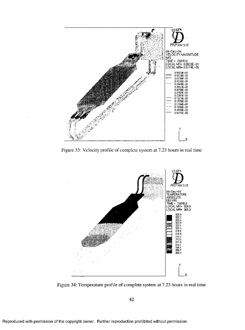
Figure 30: Temperature profile of complete system at 6 hours in real tim e....................... 39Figure 31: Velocity and temperature profiles of solar collector at 6 hours in real tim e... 40 Figure 32: Velocity and temperature profiles of water reservoir at 6 hours in real time.. 41Figure 33: Velocity profile of complete system at 7.23 hours in real tim e ........................ 42Figure 34: Temperature profile of complete system at 7.23 hours in real tim e..................42Figure 35: Velocity and temperature profiles of solar collector at 7.23 hours in real time

.................................................................................................................................... 43Figure 36: Velocity and temperature profiles of water reservoir at 7.23 hours in real time

.....................................................................................................................................44Figure 37: Velocity profile of complete system at 10.5375 hours in real tim e ..................45Figure 38: Temperature profile of complete system at 10.5375 hours in real tim e 45Figure 39: Velocity and temperature profiles of solar collector at 10.5375 hours in real

tim e ............................................................................................................................46Figure 40: Velocity and temperature profiles of water reservoir at 2 hours in real time.. 47Figure 41: Velocity profile of complete system at 12 hours in real tim e ........................... 48Figure 42: Temperature profile of complete system at 12 hours in real tim e.....................48Figure 43: Velocity and temperature profiles of solar collector at 12 hours in real time. 49 Figure 44: Velocity and temperature profiles of water reservoir at 12 hours in real time 50 Figure 45: Collector outlet behavior for the natural convection open loop solar water

heating system...........................................................................................................52Figure 46: Reservoir mean temperature for the natural convection open loop solar water

heating system...........................................................................................................53Figure 47: Velocity profile of closed loop solar water heater after 1.5 hours in real tim e54 Figure 48: Temperature profile of closed loop solar water heater after 1.5 hours in real

tim e ............................................................................................................................ 55Figure 49: Velocity and temperature profile in solar collector after 1.5 hours in real time

.....................................................................................................................................56Figure 50: Velocity and temperature profile of water reservoir after 1.5 hours in real time

.....................................................................................................................................57Figure 51: Velocity profile of closed loop solar water heater approximately after 12.22

hours in real tim e ..................................................................................................... 58Figure 52: Temperature profile of closed loop solar water heater approximately after

12.22 hours in real tim e .......................................................................................... 58Figure 53: Velocity profile of closed loop solar water heater after 3.5 hours in real time

without heat lo ss ...................................................................................................... 60Figure 54: Temperature profile of closed loop solar water heater after 3.5 hours in real

time without heat lo ss ............................................................................................. 60Figure 55: Velocity profile of closed loop solar water heater after 3.5 hours in real time

with heat loss.............................................................................................................61Figure 56: Temperature profile of closed loop solar water heater after 3.5 hours in real

time with heat lo ss ...................................................................................................61Figure 57: Velocity and temperature profile of solar collector after 3.5 hours in real time

without heat lo ss ...................................................................................................... 62Figure 58: Velocity and temperature profile of solar collector after 3.5 hours in real time

with heat loss.............................................................................................................63

V lll


Figure 59: Velocity and temperature profile of water reservoir after 3.5 hours in real timewithout heat lo ss ...................................................................................................... 64

Figure 60: Velocity and temperature profile of water reservoir after 3.5 hours in real timewith heat loss.............................................................................................................64

Figure 61: Velocity profile of closed loop solar water heater after 1.5 hours in real tim e65 Figure 62: Temperature profile of closed loop solar water heater after 1.5 hours in real

tim e ............................................................................................................................66Figure 63: Velocity and temperature profile for solar collector after 1.5 hours in real time

.....................................................................................................................................67Figure 64: Velocity and temperature profile for water reservoir after 1.5 hours in real

tim e ............................................................................................................................ 68Figure 65: Velocity and temperature profile for water reservoir after 12.22 hours in real

tim e ............................................................................................................................ 69Figure 66: Velocity profile of closed loop solar water heater after 1.5 hours in real time70 Figure 67: Temperature profile of closed loop solar water heater after 1.5 hours in real

tim e ............................................................................................................................ 70Figure 68: Velocity and temperature profile for solar collector after 1.5 hours in real time

.....................................................................................................................................71Figure 69: Velocity and temperature profile for water reservoir after 1.5 hours in real

tim e ............................................................................................................................71Figure 70: Velocity and temperature profile for solar collector after 12.22 hours in real

tim e ............................................................................................................................ 72Figure 71: Mass flow rate at the collector top section for different cases...........................73

I X


ACKNOWLEDGEMENTS

I would like to acknowledge the help and esteemed guidance of the Project

Investigator and my academic advisor Dr. Samir Moujaes for providing supervision and

assistance with every step of the work.

I would like to thank Dr. William Culhreth, Dr. Mohamed Trahi a and Dr. Samaan

Ladkany for there support.

I would like to thank the Department of Mechanical Engineering for funding the

project for purchase of extra licenses of Star CD.

Support from the Voss Lytle and Jaime E. Comhariza from NSCEE is greatly

appreciated.


CHAPTER 1

INTRODUCTION AND BACKGROUND

1.0. Solar Domestic Water Heating Systems

Solar domestic hot water systems are widely used in countries like Australia,

Israel and Jordan, and have tremendous potential in other developing countries [I]. These

systems operating costs is negligible as compared to conventional hot water systems [2].

The initial cost of these systems heing too high is one of the main stumbling blocks in the

more common usage of these systems.

1.1. Classification of solar water heating systems

1.1.1. Natural circulation solar water heaters

In natural circulation solar water heaters the fluid is circulated by natural

convection. The sketch of conventional natural circulation solar water heater is shown in

figure 1. The collector absorbs the heat from the sun. The thermal energy absorbed in the

collector fluid is then transferred to the circulating fluid, which creates the fluid density

difference between the collector fluid and fluid inside the storage tank. This density

difference results in a buoyancy effect and hence circulation of fluid inside the solar

water heater. During the night there is a possibility of flow reversal in solar collector i.e.

water enters through the top of the collector and leaves from the bottom of collector,

hence losing the heat to the atmosphere. Thus a check valve is provided in order to

I


prevent this effect of nocturnal radiation on the solar water heating systems. The most

important parameters that controls the flow rate in a natural circulation solar water heater

is the location of storage tank above the collector and pipe sizing and the amount of

radiation absorbed by the collector, which varies throughout the day and year.

ToLoad

StorageTank

Frommains

SolarCollector

Figure 1: Direct type Natural circulation solar water heater

1.1.2. Forced circulation solar water heater

The forced circulation solar water heater uses a pump for the circulation of fluid

in the solar water heater. A pump is normally controlled by a differential temperature-

sensing controller that turns on the pump on when the collector outlet temperature is

greater than the temperature in the bottom of the tank [2]. Thus the flow inside the forced

circulation can be either mixed convection or forced convection depending on the

Reynolds number at which the system is operating. Thus the pump increases the initial


cost as well as the operating cost of the system. The sketch of forced circulation solar

water heater is shown in figure 2.

To Load

SolarCollector Storage

Tank

To MainsPump

Figure 2: Direct type Forced circulation solar water heater

Solar domestic water heating systems can also be classified as direct or indirect

type. In direct type systems the heat is transferred from the collector to domestic water

directly. The system in figures 1 and 2 are examples of direct type solar water heaters. In

the indirect type the heat is transferred from the collector to the water using an

intermediate fluid and an indirect heat exchanger. The indirect type systems are used

generally in geographical regions with cold weather conditions. One such intermediate

fluid is a mixture of water and ethylene glycol, which can operate in cold temperature

without freezing depending on the concentration of ethylene glycol. The indirect type

solar water heating systems is shown in figure 3.


ToLoadSolar

CoLLectorStorageTank

From.

Pump

Figure 3: Indirect type solar water heating system

Several numerical and experimental studies have been performed on both natural

(thermosyphon) and forced circulation type of solar water heating systems which are

briefly discussed below.

The numerical studies consist of developing a model of solar water heating

system and conducting the simulations. It was observed that major work has been done

using TRNSYS simulation program in the past, some of which are given in brief as

follows:

A study was conducted using TRNSYS simulation program for Los Angeles for

comprehensive assessment of the impact of most of the design parameters on efficiency

and solar fraction to provide guidance on the “optimum” value for each with an objective

to maximize annual performance of a domestic thermosyphon solar water system. [4].

A study was conducted using TRNSYS simulation program in which a model of

thermosyphon solar water heater was developed to determine the instantaneous collector

efficiency as a function of the time of day and correlated with the thermosyphonic-flow


rate of water and the temperature difference between the water at the collector’s inlet and

outlet. The model was also used to predict the monthly and yearly solar contribution of

the system for two different load profiles. [5].

A study was conducted using TRNSYS program in which model of forced

circulation solar hot water system was used to correlate the performance and cost

effectiveness of the system with a number of key design criteria (e.g. the collector to

consumer factor (FCC) and the collector to load factor (FCL)) with an objective to

optimize the design criteria of solar hot water (SHW) systems intended for residential

hotel applications. [3].

A study of thermosyphon systems was done to determine collector flow rates and

thermal stratification in storage tanks, to assess how these flow rates relate to those used

in pumped systems with various control strategies, and develop a design method for

thermosyphon system based on the equivalent flow rates for pumped system. Thermal

stratification in the storage tank was accounted for through use of a modified collector

heat loss coefficient. Comparison was made between the annual solar fraction predicted

by design method and TRNSYS simulations for a wide range of thermosyphon solar

DHW systems. [1].

The authors developed a computationally efficient high-level model for

simulating indirect thermosyphon solar energy water heaters to study the characteristics

of hot water stored under steady state and real operating conditions. The results indicated

that the degree of stratification in a hot water store was correlated with the ratio of

colleetor to load volume flow [6].


The authors derived a more general and realistic model in which the loss of heat

through the storage tank is considered and the variation of solar radiation, ambient air

temperature and temperature of the cold feed water was taken into account. A transient

analysis of forced circulation solar water heating system with and without heat

exchangers in the collector loop and storage tank was presented. Exact solutions of

different cases were presented and analyzed [7]

Authors presented details of experimental observations of temperature and flow

distribution in a natural circulation solar water heating system and its comparison with

the theoretical models and showed the measured profile of the absorber temperature near

the riser tubes conforms well to the theoretical models. The mean absorber plate

temperature and mean fluid temperature during a day has been estimated and compared

with theoretical models. Measurements of glass temperature were also carried out [8].

An experimental study was conducted by authors to compare the performance of

natural and forced circulation domestic solar water heaters. The main parameters

calculated are top, back, and overall coefficients, the heat removal factor, the efficiency

factor the useful energy gain and instantaneous efficiency. [9]

A test conducted on built-in solar water heater which was tested both

experimentally and theoretically under three different operation modes namely; no flow,

continuous flow and intermittent flow. It was found that the average efficiency (t)) of the

system is of maximum value under the continuous flow condition, while it has a

maximum hourly efficiency under the intermittent flow condition [10].

Authors conducted an analytical experimental investigation into the temperature

field inside the hot water storage tank of a solar collector on a transient two-dimensional


semi-infinite cylindrical length model with time-and-space boundary conditions

dependency was selected. Conduction and convection heat transfer modes in the axial

direction together in conduction in radial direction were neglected. Temperature profiles

in the axial direction of a cylindrical storage tank were assumed to be linear [11].

Author presented mathematical model for the transient conjugated behavior of hot

water storage tank having finite wall thickness and obtained closed form solution for the

temperature field within the tank while considering the axial conduction of heat in both

fluid and solid wall and the heat capacity of the solid wall. Results showed that finite wall

thickness tends to decrease the thermal stratification within the tank and this effect

becomes less apparent at high Peclet numbers [12].

Besides this several other experimental and numerical research work on solar

water heating systems were done by Adnan M Shariah and A. Ecevit [13], Eng. Malek

Kabariti and Eng. Yaser Mowafi [14], l.M. Michaelides and D R. Wilson [15], Soteries

A. Kalogirou, Sofia Panteliou and Argiris Dentsoras [16], B. Norton, P.C. Eames and

S.N.G. Lo [17], M. Altamush Siddiqui [18]. Also from literature only one research paper

was found in which the CFD program (FLUENT) and a solar simulator, for designing a

solar water heater [19]. CFD transient simulations were carried out by him using small

time step of 10 seconds and a set of body fitted computational grids (1770*4740 nodes).

FLUENT results were the verified against indoor testing employing a solar simulator. He

mentioned it that it took a long time for him to get the results.


1.2. Significance of work

Residential hot water use represents a large proportion of residential energy use.

Thus the residential energy usage can be reduced significantly if solar water heating

systems could be effectively used for water heating. Till now, the initial cost of the solar

water heating systems has been the major stumbling block for the usage of solar water

heater [2], Most of the studies carried out in past on solar water heating systems are either

experimental or numerical which involves significantly high costs. Also the majority of

past studies were condueted on plate and tube type of collector where the major heat will

transfers from the part of the flat plate between the tubes to the water. The water flow

through a flat eross sectional channel instead of flat plate and tube type of arrangement

can reduce the heat losses from the solar collector. In two decades CFD has emerged as a

powerful simulation technique for the cost effective study of various heat transfer and

fluid flow problems with reasonable accuracy as compared to other approaches, but the

study of solar water heating systems using this technique was very rare.

Hence the present study using CFD of three dimensional model of natural

convection open loop and forced convection closed loop solar water heating system will

add to the literature and potential physieal insight in this area. This study will concentrate

on a natural eonvection open loop and foreed convection closed loop system simulation.

The solar eollector studied is of truly flat shape, which would increase the amount of heat

transfer from collector to the water as compared to flat plate and tube type design. This

study can be extended further to optimize different parameters and materials for the

optimum design and eost reduetion of both natural and forced conveetion solar water


heaters and thereby would further help to inereasing the usage of solar water heaters

which are still not that popular due to high initial costs.


CHAPTER 2

MODEL DESCRIPTION AND NUMERICAL METHOD

This chapter provides information on the working theory behind the simulation

package used to model the solar water heating systems considered for simulations. The

chapter is split into two subchapters. The first part provides a detailed deseription of the

physical model of the solar water heating systems used for the present study. The second

subchapter presents the details of numerical model that were used for the present study.

2.0. Model Deseription

The physical model of the solar water heater used for the CFD simulation consists

of flat surface solar collector and water reservoir connected by a piping system. The solar

collector considered here is of truly flat shape rather than a conventional fin and tube type

colleetor. The fin and tube type collector usually exhibit larger heat loss along the upper

faee of the eolleetor than flat ones beeause the average temperature on the flat surfaces is

lower. Also as the pipes are connected to the flat plate through brazing the amount of heat

transferred to water depends on the conductivity and quality of the brazing. Hence in

order to maximize heat transfer from collector to water an alternative design of truly flat

shaped eolleetor shown in figure 4 (dimensions shown in figures 6 and 7) is used for CFD

simulation where all the heat eollected by eollector will be directly conducted to water

flowing below it.

10


The solar collector was considered to be south facing with an inclination of solar

collector (34.759 Deg) from the horizontal was considered for the Las Vegas, NV for the

month of June [2], The flat plate collector is connected to pipes with a conical section

shown in figure 4 (dimensions shown in figures 6 and 7). The conical section is designed

to ensure that the water flows evenly through the cross section area of solar collector and

back into the pipes from top of the collector. The pipes are further connected to the water

reservoir from where water can be tapped for usage depending on load.

Solar Collector

ConicalSection

Figure 4: Conical Section that connects the solar collector and pipe

2.0.1. Natural convection open loop solar water heating system simulation

The open loop system was used to perform simulations for natural convection

solar water heating system (figure 5) to make it realistic for residential applications. The

top surface of the solar collector receives the heat from the sun. No glass cover or metal

11


surface is simulated in this effort. A certain amount of solar heat flux is imposed as input

on the upper most surface of the collector. This heat is then convected to the water

flowing in the rectangular channel. The sides of the collector, which exhibit a relatively

small area, are assumed to be adiabatic as is the backside of the collector.

The heat gained by water as it flows results in the change of density of water. It is

this density difference due to which the water flows from collector to the reservoir and

back. As the time increases the closed loop of water flow is set up between the collector

and reservoir which results in rise of temperature of water inside the reservoir. In the

effort to make this system realistic for residential application the simulation was

programmed so that water was tapped at different times a day namely interval I and 2.

The schedule for interval for tapping hot water from reservoir is: Interval 1-20 min from

13:00 pm to 13:20 pm. Interval 2- 20 min from 17:00 pm to 17:20 pm. The inlet is

introduced from the bottom and outlet from the top to tap into the hottest water layers of

the reservoir. The dimensions for this system is same as shown in figures 6 and 7 except

that the inlet and outlet pipes are introduced at the top and bottom of the water reservoir.

12


Sdar Coüector

WaterReservoir

A= Outlet Pipe (Dia. = 12.5mm) B=InletPipe (Dia. =12.5mm)

Figure 5: Natural convection open loop solar water heater used for CFD simulations

2.0.2 Forced convection closed loop solar water heating system simulation

A closed loop system simulations for the forced convection solar water heating

system was performed. This meant that no make up water was used in the simulation and

no hot water was tapped from the system. This is not how the forced circulation solar

system is run on a daily average, but the simulation results are useful to shed some light

on the general performance of the system. It also gives some preliminary numerical

values of what to expect when a more realistic system is studied.

13


The figures 6 and 7 show the diagram and dimensions of the closed loop system.

This study can help further to simulate the forced convection solar water heater for

different Reynolds number and there performance comparison.

F r o n t V ie w

A l l d im e n s io n s i n m m

Figure 6: Front view of closed loop solar water heating system with dimensions

T o p V i e w

NO-C)

CDCDND

1200 CDCDCO

CDr o

:

A l l d im e n s io n s in tn m

Figure 7: Top view of closed loop solar water heating system with dimensions

14


2.1. Introduction to Computational Fluid Dynamics (CFD) Simulations System

A STAR-CD program is used for this study. The code comprises of the main

analysis code STAR (Simulation of Turbulence in Attributed Regions), and the

preprocessor and post-processor code, PROSTAR. STAR-CD is a powerful CFD tool for

thermo-fluids analysis and has been designed for use in a Computer Aided Engineering

environment. It is a finite volume code, developed for the calculation of fluid flow, heat

and mass transfer and chemical reaction in industrial and environmental applications. Its

main attributes include:

• A self-contained, fully-integrated and user-friendly program suite comprising pre

processing, analysis and post-processing facilities

• A general geometry-modeling capability that renders the code applicable to the

complex shapes often encountered in industrial applications

• Extensive facilities for automatic meshing of complex geometries, either through

built-in tools or through interfaces to external mesh generators such as SAMMTM

and ICEM CFD TetraTM.

• Built-in models of an extensive and continually expanding range of flow

phenomena, including transients, compressibility, turbulence, heat transfer, mass

transfer, chemical reaction and multi-phase flow

• Fast and robust computer solution techniques that enhance reliability and reduce

computing overheads

• Easy-to-use facilities for setting up and running very large CFD models using

state-of-the-art parallel computing techniques

15


• Built-in links with popular proprietary CAD/CAE systems, including

PATRANTM, IDEASTM and ANSYSTM

STAR, written in FORTRAN 77 and C, operates by solving the governing

differential equations of flow physics by numerical means on a computational mesh.

PROSTAR is an interactive, command-driven, combined pre-processor and postprocessor

whose main functions include geometry modeling and mesh generation, problem

specification, results manipulation and display, file control, and links to external

CAD/CAE systems. The governing equations used by STAR-CD [20] are given below:

The mass and momentum conservation equations solved by STAR-CD for general

incompressible fluid flows and a moving coordinate frame ( ‘Navier-Stokes’ equations)

are, in Cartesian tensor notation:

Mass conservation

1 ( 1) g cV CT

Momentum conservation

+ ; = + (2)

Where t. time

X i : Cartesian coordinate (i=l, 2, 3)

ui: absolute fluid velocity component in direction x i

u- : uj-ucj, relative velocity between fluid and local (moving)coordinate frame

that moves with velocity ucj

16


p: peizometric pressure= ps -pogmxm , where ps is static pressure, po is

reference density, the gm are gravitational field components and the xm are

coordinates from a datum, where po is defined

p : density

T ij : stress tensor components

sm: mass source

si: momentum source components

yfg : determinant of metric tensor and repeated subscripts denote summation.

The specialization of the above equations to a particular class of flow involves:

• Application of ensemble or time averaging if the flow is turbulent

• Specification of a constitutive relation connecting the components of the stress

tensor Xy to the velocity gradients

• Specifications of the ‘source’, si, which represents the sum of the body and other

external forces, if present.

In case of laminar flows, STAR-CD is applicable to Newtonian fluids that obey the

following constitutive relation:

where p. is the molecular dynamic fluid viscosity and bij, ‘Kronecker delta’, is unity

when i= j and zero otherwise, s ÿj, the rate of strain tensor, is given by:

i+ (4 )

17


For turbulent flows, w„ p and other dependent variables, including Xÿ, assume their

ensemble averaged values (equivalent to time averages for steady-state situations) giving,

or equation 28:

where the u' are fluctuations about the ensemble average velocity and the over bar

denotes the ensemble averaging process. The rightmost term in the above equation

represents the additional Reynolds stresses due to turbulent motion. These are linked to

the mean velocity field via the turbulence models.

Heat transfer in STAR-CD is implemented through the following general form of the

enthalpy conservation equation for a fluid mixture:

Here, h is the static enthalpy, defined by:

( 7 )

and T: absolute temperature

Cp : Mean constant pressure specific heat at temperature T

Cp : reference specific heat at temperature To

Sh: energy source

h(: thermal enthalpy

It should be noted that the static enthalpy h is defined as the sum of the thermal

and chemical components, the latter being excluded as it is not pertinent to the analysis

here.

IS


The governing equation for thermal enthalpy is given by:

!& Of m , cY ' ovy

Here, h, is the thermal enthalpy, defined by

A, (9)

and Fhtj : diffusional thermal energy flux in direction xj

A governing equation for total thermal enthalpy (H) may be formed by summing an

equation for mechanical energy conservation and static enthalpy equation:

where, H - ( l /2 ) u i + h (11)

2.2. Numerical Model

2.2.1. Natural convection open loop solar water-heating system simulation

The numerical model for the solar water heater is 3-D with total number of

nodes as 323407 for open loop system. The type of cell used was tetrahedral with a cell

size of approximately 2.5 mm for inlet and outlet pipe, 5 mm for the solar collector and

the piping system and 16 mm for reservoir. The 3-D model was made in a CAD program

and was meshed in the Star CD. Figure 8 and 9 shows the mesh generated by Star CD for

the CFD simulations. The time step used for simulations was 15 seconds and the

simulations were run for real-time from 0700am to 1900pm.

19


Figure 8: Mesh for pipe, conical section and solar collector used for CFD simulations

Figure 9: Mesh for reservoir, inlet pipe and outlet pipe used for CFD simulations

20


The boundary condition for different sections of system is as follows:

1. Solar collector: The top surface of the solar collector was supplied with a boundary

condition of heat flux with respect to time (figure 10) that will be acting as solar

insolation [21].

2. Pipes, conical section, water reservoir and for bottom and side parts of the collector are

supplied with adiabatic boundary condition.

3. The inlet pipe is forced with the flow rate of 3 GPM, which simulates the hot water

usage twice a day as shown in figure 11 schedule.

4. Outlet pipe is supplied with boundary condition to satisfy continuity equation.

The thermal performance of the solar water heater was obtained by simulation from

0700am to 0700pm.

Solar Insolation vs Time

à- 1 M 1 2 0 0 -

^ 1000 -

200 -

8 8G)

8CO

8 8CD

8 8G)

8O

Oc\i

o00

Time

Figure 10: Solar insolation used for CFD simulation from 0700 to 1900

21


Inlet Water Velocity vs. Time

« 0.8

> 0.4

Figure 11 : Profile of the inlet water velocity vs. time for hot water usage from 0700 to

1900

2.2.2. Forced convection closed loop solar water-heating system simulation

The numerical model for the forced convection solar water heater is a 3-D

transient with total number of nodes as 205,000. The type of cell used was tetrahedral

with a cell size approximately 5 mm for the collector and 20 for the reservoir. The 3-D

model was made in a CAD program Solid Works and was meshed in the Star CD. The

time step used for simulations was 15 seconds for all the cases and the simulations were

performed for three different Reynolds numbers 500, 1000, and 1500.

The boundary condition for different sections of system is as follows:

1. Solar collector: The top surface of the solar collector was supplied with a boundary

condition of heat flux with respect to time (figure 10) that will be acting as solar

insolation [21].

2. Pipes, conical section, water reservoir and for bottom and side parts of the collector are

supplied with adiabatic boundary condition.

22


3. Source momentum was supplied to simulate the effect of pump in the pipe section just

below the water reservoir.

The numerical scheme used for both solar water heating systems are discussed briefly as

follows:

1. A Boussinesq approximation was used to define density as a function of

temperature. It was used to take into account the potential buoyancy effects in the

reservoir that occurs due to mixing of hot water from collector and the cold water

inside the tank. For natural convection case this is the main condition for setting

up the flow inside the loop. Whereas in forced convection case its supplied to

study the effect of mixed convection which may occur at low Reynolds number

2. PISO Algorithm was used for solving the transient problem.

3. AMG (Algebraic Multigrid) approach was used for solving matrix equations.

4. The numerical simulations were run in a transient mode for 12 hours of daytime

i.e. from morning 0700am to evening 0700pm.

For more details about the numerical scheme please look in [20].

23


CHAPTER 3

RESULTS AND DISCUSSIONS

This chapter provides a detailed overview of the results of runs from simulations

for natural convection open loop solar water heater model and forced convection closed

loop solar water heater model. The numerical accuracy for the natural convection system

was checked by satisfying the continuity equation at the top and bottom section of

collector and reservoir respectively. The accuracy was found to be within 2.59 % for the

collector and 0.32% for the water reservoir for the 4 hour of real time simulation data

wherein the flow has been developed between the solar collector and water reservoir. The

discussion shows the effect of the solar radiation on the temperature, velocity and mass

flow rate of water in natural convection solar water heater as a function of time.

The discussion also shows velocity and temperature profiles and the effect of

variation of Reynolds number on each of the above parameters for the forced circulation

closed loop system. The parametric study was performed on this model for three different

Reynolds number i.e. 1500, 1000 and 500 in the laminar flow regime. The separate

simulation run was performed on closed loop system for 1500 Reynolds number in which

the solar flux falling on the solar collector was considered to include the heat losses from

the solar collector from top and sides. And the results of this run were compared with the

runs with model that doesn’t include any heat losses from the collector. The closed loop

24


system was also checked for numerical accuracy by checking the whether the system

satisfies the continuity equation. The accuracy for closed loop system was found to be

within 0.34 % for the collector. Finally the discussion explains the comparison between

current study and the relevant literature.

3.0. Natural convection open loop solar water heating system

This section shows the results of the simulations at 2, 4, 6, 7.23, 10.5375 and 12

hour data in real time starting at 0700AM.

3.0.1. 2 hour real-time simulation data (0900AM)

Figures 12 and 13 show the velocity and temperature profile of the natural

convection solar water heater. It can be observed that as the temperature of the water has

rise from 305 K to 318.7 K in two hours of real time. As there is no momentum source in

natural convection case, the water velocity slowly rises as the water gains heat from the

solar collector. The gain in heat results in the density difference between the water at the

top of the collector and the bottom of the reservoir because of which the water flows from

the reservoir to the collector and vice versa which results in flow of water from the

collector to the water reservoir.

25


y

: \ i W # "

'V

gar*

PRO'AM 3.10

M-Oec-O-iVELOC<TY WA<aiTlJDEM 'STIM E . 7200C0 LOCAL MX- 0O Z 8E -01 LOCAL Q4Z83E-06

04KK-0I 0 4 0 ÎS L -0 1 0 J 7 ! C { - 0 1

0 J 4 û 1 t - 0 ) 030KE-OI 0?WE-(ll0M7*OtIMEOIKSE IWW 0O7E OTZMf OtIWE-OZ OXME'OZ OiSME-OI,

I---%

Figure 12; Velocity profile of complete system at 2 hours in real time

V f "

PRO*AM 3,10

0 9 -0 6 0 - 0 4TEMPERATUREABSOLUTEKELVINTIME - 7200,00 LOCAL M X- 318,7 LOCAL M N- 30S.0

31 ! 8

3 10 9

Figure 13: Temperature profile of complete system at 2 hours in real time

26


Figure 14 and 15 shows the temperature and velocity profile of the solar collector

and the water reservoir. It can be clearly observed that as the water gains heat as it flows

over the solar collector and flows towards the reservoir. As the water from the collector is

at the higher temperature than the water reservoir, it moves upwards after entering the

reservoir. Then after reaching the opposite end it starts moving down and mixes with the

cold water in the reservoir resulting in the rise if water temperature inside the reservoir.

This relatively hot water rises inside the reservoir and moves upwards and gets

accumulated in the top layer of the reservoir as can be observed in the figure 15. And thus

the water according to the temperature is stratified inside the reservoir with high

temperature in the top and lower temperature at the bottom. Figure 15 also indicates the

section of collector for figures 17, 18 and 19.

0

j Vi'-S' li'-“ , Î .

O-OgC-04vEiocrrv MAONrnjOE W5TIME" 7200m lO C A l MX" 0 3 3 7 ^ -0 1 lO CA lkM "0.7207E-(l4

OKME-OI83WTE-01OZTMt-OI

OIMIE-OIOtKiE-OI

Q55S9E-K8 « 3 5 E -K07ai7E-W

H >

-o

P R O * A M 3 . IQ

og-Oec-04.7URE

- 7 2 0 0 . 0 0 lOCAlMX. 318 7 lOCAlf/N" 3108

311.7316 2 317,6 3 1 7 6 3 1 6 5 315 3 3 1 5 3 314 9 314 2 313 6 3131 312 5 311 3 311 4 3 1 0 8

Figure 14: Velocity and temperature profiles of solar collector at 2 hours in real time

27


AM 3.10

OamfAGNiTllCÆ _ |^m'Ti I'lOCAl».$(

. 7ZOOOO - M%.0.X4?E."01 , 0 154)E-Q403W.:t.0l03WE-01OAAE-mD2X$f-0i0%9W"0i

" V r 01

DfC-04 /PER A TIPE

/T t.

7ZU0.00 ..O CA l M X . 3165 LOCAL 3119

C.e' — Oiw

L : .

AM 3.JO

Figure 15: Velocity and temperature profiles of water reservoir at 2 hours in real time

Figure 16 and 17 shows the section of reservoir at which water enters the

reservoir. It can be clearly seen that the water moves upwards and then to the opposite

end inside the reservoir, it is then diverted in the different directions along the surface of

the reservoir.

28


I'.k - : ' ' '

A M 3 10

m O C i ’Æ'* M A G N ITU D E

TIM E - 7ZOOOO LOCAL M X . 0 3 4 8 Z E - 0 I LOCAL 0 4 e 4 2 { -0 4

0>1S?E-01 Q3Z33E-01 0Z3ME-01CZ737E-050Z4WE-0102240E-0101932E-Q1017436-01Ç >495E-0'l

0 1247E -01- 0Wa2E-03074986-02

0X1156-0? 0A 32E -0T 0 4 t* 1 E 'W

Figure 16: Velocity profile at the section normal to water reservoir and connecting pipe

from collector at 2 hours in real time

.G'AMSTO

! C - 3 - 0 e c - G 4 ; T E M P E R A T U R E

n W E . 7200jQ0 lOCAlM X" 3168 LOCAL k?*- 3142

Figure 17: Temperature profile at the section normal to water reservoir and connecting

pipe from collector at 2 hours in real time

29


Figure 18 shows the temperature profile at the middle of water reservoir. It can be

observed that there are some localized hot zones that depict the zone from which the hot

water rises towards the top of the reservoir. It also shows the mixing and heat convection

from hot water to the relatively cold water at this section.

©PRO*AM 3.10

<3@-Dec-04T E M P E R A T U R EABSOLUTEKELVINTîME - 7200.00 LOCAL KW. 3 M a LOCAL Xiff. 312 7

314 0 314 03131 3138 313 7 3138 3135313 431333132 313 1 313 0 3129 312 9 3IZ7

Figure 18: Temperature profile at the section normal to middle of water reservoir at 2

hours in real time

Figure 19 shows the temperature at section located at the bottom of the water

reservoir. It can be observed that there are some localized hot zones here from which the

heat is convected from the hot water to the cold water at this section. As the section is at

the bottom the temperature difference at this section is relatively smaller to the other two

sections which are at the middle and top of the reservoir.

30


P F 5 0 * A M 3 -1 0

O9-Dec-04 TE7/PERATUPE ABSOLUTE KELVIN TIME - 720080 LOCAL XK» 3123 LOCAL k « . 3128

312 8

312 J

Figure 19: Temperature profile at the section normal to bottom of water reservoir at 2

hours in real time

Figure 20 and 21 shows the velocity and temperature profile of the conical section

at the intersection between pipe and solar collector where the cold water enters the solar

collector. It can be observed that as the water enters the conical section it spreads and

moves towards the collector. There are some localized flow zones where there is some

eddy formation. The temperature of the water rises as it leaves the conical section and

comes in contact with the solar collector.

31


l î M P

PRO'AMSIO

09-Dec-MVELOCITY MAGNITUOE NVSTIW E" 7200:00 lO C A l 0.3939E-01 lO C A l W f-0.»2$8C-(W

OKME-OI 0W73E-0I03037E -01

02*1«E-OI0 2 W E - 8 I022M E -O I0I97AE-O1C l t 3 ) E '0 l01412E-81

O I13IE -O IÛ $% 6E -02 OXME.O:

— oerwE-M

Figure 20; Velocity profile of the conical section at the bottom of collector at 2 hours in

real time

STA^

'éSSSSi

PRO’ AM 3.10

09- D e c - G 4TEMPERATUREABSOLUTEKELVINTIM E" TZCmClOLOCAL MX" 318.7 LOCAL M N- 310.8

3153

311 431BS

Figure 21: Temperature profile of the conical section at the bottom of collector at 2 hours

in real time

32


Figures 22 and 23 shows the velocity and temperature profile of the conical

section at the intersection between pipe and solar collector where the hot water leaves the

solar collector. It can be observed that there is a single localized flow zone. There is

stagnation of water inside this zone and water flows around it to enter the pipes

connected to the conical section.

ST A p t

/ \

Mr

39E-0I -04

PRO"AM3.10

0 9 - D e c - 0 4V E L O C IT Y M A G N IT U D E M/5T I N Æ . Z20Q.O0 LOCAL MX- 0.39: LOCAL W'l" 0.821

0 3933E-0Î---- 0 3J7BE-01

0.309’ E-I)1 02S1SE-01 DJS35E-B1 0e?55E -01 01974E-01 0.1693E -ei

01412E-01 0.n31E-O l 0 85W E -02 0 5639E-0i

0 2891E-S2 0 .8 2 M E -0 4

Figure 22; Velocity profile of the conical section at the top of collector at 2 hours in real

time

33


PRO* AM 3,10

0 9 -D e c -0 4 TEMPERATURE ABSOLUTE KELVIN Tlk€. 72oaoo LOCAL MX- 318.7 LOCAL MM- 310.8

3 !S S

Figure 23: Temperature profile of the conical section at the bottom of collector at 2 hours

in real time

Figure 24 shows the temperature profile inside the solar collector at the sections a,

b and c shown in figure 14. All of these sections are located at the section where there is

no change in cross section area across the collector. It can be observed that as the water

gains heat as it moves along the length of the collector.

34


PM)'*M3.I0

K-Dci-'WIt'/cicaTlREfPXAlTE1IM. %0XMI !OC6| rA (' 3143 iO C tlf /N - 311.8

114)114))I4«)|j*)D*11)4M):

PRO*AM 3.10

O -D e c -0 4T E M P E R A T U R EAGsoimtKELVINT « Æ - 720000 LOCAL ;.M« 316.0LOCAL M .S'. 311,8

)D1>12)ill!

)U«.117 1

A V .3 10

Dec-o; -:V:'cR4TL<?E

- vE. ?roci!0] ID C A IM X - 3 1 8 0 L O C A L 3 1 1 0

5160 5l7t 5172 51C7 316) 3 15 » 3154 fisc 514 5 3M1 3 1 )4 31)2

3111

Figure 24: Temperature profile of the collector at various sections (a- bottom, b-middle

and c-top section) at 2 hours in real time

3.0.2. 4 hour real-time simulation data (01100AM)

Figures 25 and 26 show the velocity and temperature profile after 4 hour of real

time simulation. It can be observed that as the daytime increases there is increase in

velocity as well as in the temperature of the solar collector.

35


1 PRO* AM 3.10

0 9 -D e c -0 4VELOCITY MAGNITUDE M /ST IM E - M 400.0 LOCAL M X - 0 .6029E -01LOCAL M N - 0 .1540E -04

0.6023E-01 0SS98E -01 0.5168E-01

0.4737E-01 04307É-G1 0.3876E-01 0.344 6E-01 0.301 5É-01 0 25S5E-01

0.21$4E-01- ..... 0.1724E-01^ 01293E-01 0.$62SE-02' ' 0.4321E-02 01541E -04

Figure 25: Velocity profile of complete system at 4 hours in real time

P R O 'A M 3.10

0 9 - D e c - 0 4TEM PERA TU REABSO LU TEKELVINTIM E - 14400.0 LOCAL M X - 3 4 6 .7 LO CA L M N - 30 5 .0

3 4 5 7342-8339 9

334.1

3 2 8 .33 2 5 43 22 53 1 9 53 16 63 13 73 1 0 8307 .93 0 5 0


From figure 27 it can be observed that there is not only increase in temperature of

water inside the collector but also in the temperature difference across the collector which

36


shows the increase in the heat gained by water due to increase in the solar heat flux acting

on the collector. There is also increase in the flow velocity inside the collector.

I 1I P PO 'A M S .IO

|e9-c-5c-04 VELOCITY MAGNrrUDETIME - 14400.0 LOCAL WX- 0.5S47E-01 LOCAL 051686-04

Q5^151E-01 047S5E-01 04353E:-01 Q39ME-01 0 J5WE-CI 0372E-01 0 2776F-01 0 23M E-01 01M 4E -01 Û15ME-Û1 01%936-01

0401ÙS-0&OSTëBE-iM

l»â

©P R O ‘ A M 3 .1 0

m-Dcc-04T E M P E R A T U R EABSOLUTEKELVINTIME - Î440&0 LOCAL 345.7 LOCAL KiN- 336.4

345.7mm 3451 3*3 734:4■Ul 7341 n340 4 339 7 3)9 0 3104 337 7 33/ 0 3364

\ /

z__%


From figures 28 it can be observed that there is significant rise in temperature of

water inside the reservoir. The flow velocity inside the reservoir has also increased

resulting in proper mixing and stratification inside the reservoir.

37


0PRcxAMaioC3-0*C-<MVElOOrfMÀQNlTlJDELV5TiME - 1lOCA. * II 1 l f - 0 4

I— 04 * n 1

©PRO*AM310

æ -D sc -0 4TEMP£RAUiF€ABSOlUrEKELvm;T ;M E • ! 4 4 0 0 0LOCAL }.<» 342, LOCAL W f. 337.

14: «542 5 3421 341 ?341 3 WÎ 0 3406 34GZ 333 0 333 5 339 1 338 7 330 3 333 C 337 6


3.0.3. 6 hour real-time simulation data (0100PM)

Figures 29 and 30 show the velocity and temperature profile at 1:00 pm real-time.

It can be observed that there is hot water coming out of the solar water heater from the

outlet due to the imposed inlet condition at the inlet. The mass flow rate of the water from

outlet is relatively higher than the operating flow rate inside the solar water heater. In the

temperature profile it can be clearly observed that the temperature of cold water entering

the water reservoir results in localized stratification at the bottom of the tank from the

water at higher temperature inside the reservoir and the incoming water at relatively

lower temperature. It can also be observed that the temperature of water is highest on the

top of the water reservoir from where the hot water flows out for domestic usage.

38


PRO’ AM 3.10

07 -D ec -0 4VELOCIP/MAGNITUDE M !STIME - 21600.0 LOCAL MX- 7.058 LOCAL MN= 0.8984E-04

7 058 8 .554

6 .0505.546

5 0424 ,5 3 6 4 .0 3 3 3 5 2 9 3 025

- 2.5212 017 1 5 13 1 .008

■ 0 .5 0 4 3" 0 8 9 6 5 E - 0 4


P R O 'A M 3.10

0 7 - D e c - 0 4TEM PERA TU REABSOLUTEKELVINTIM E « 2 1 600 .0 LOCAL M X - 390 ,5 LOCAL MN= 304 .9

3 9 0 .53 8 4 .33 7 8 .2372.13 6 6 .0 3 5 9 ,9 3 5 3 .83 4 7 .73 4 1 .83 3 5 .43 2 9 .33 2 3 .2317.1 3 1 1 .0 3 0 4 9


39


Figure 31 shows the velocity and temperature profiles of the solar collector at 6

hours in real time. It can be observed that the collector reaches the maximum temperature

at the 6 hours as there is maximum solar heat flux acting on the collector surface.

■1

t oPKy'Ai'viî.io

VELOCITY' M A G N llU D : IW32 «00.0 ,lOCAl kK- 0.27)0 ,LCKiAL MM»

—— )Z535---->2115' ).i 56# : . .

>1 305 J.1 1 fU

— ) .9 ? { .5 Ï -8 1---3 .353’C-i3l 13Vl!IF-ni

),1 M -0

mao AM 3.10I07-C*C»04 1 TEkfSRATT.'RE IAB^CLVTE I KLELVlN I TIME - Z I WOO ) LOCAL MX- 333.5 ( L O C A L 3 4 5 5

%jw a i#cn aI ’i -*i •14a. ri t* l «3

I './ .I a 2"j"'- 3 r 3

âL J -


Figure 32 shows the velocity and temperature profile in the section of inlet and

outlet pipe of the water reservoir. From the velocity profile it can be observed that as the

capacity of tank is large, the effect of the inlet flow rate is very small on the flow inside

the tank which results in mixing and stratification inside the tank. From temperature

profile it can be observed that though at the bottom of the reservoir there is some

stratification of temperature, top of the reservoir still contains the water at higher

temperature. The top left part of the temperature profile (section ‘a’ in figure 32) shows

the higher temperature as compared to the top right part because of the effect of entering

40


hot water from collector on the top left part and outgoing hot water from top of the

reservoir.

j C ,

07-DfC-04wsri\(. 2:ew(iLOCAL 3 1 3 5 LOCAL

fNCrow1 'Ai

v S ',,"C&\.r )t»' IciîoU*f-î

î>P P O 'A M IIO

o; -D € c- o4TEMPERATUREABSOLUnKELVINTIME - Z16000LOCAL MK- 377.3LOCAL KT4- 3 0 4 3

37? 5

3B?5W2 33M 9 34(5 6 041 4 Jik :331 U320 5310 1 3WS

L


3.0.4. 7.23 hour real-time simulation data (0213PM)

Figures 33 and 34 show the velocity and temperature profile at 7.23 hour real time

data. It can be observed that after the water has been tapped at the interval 1 there is

reduction in the temperature in the whole system. Due to which the velocity and

eventually the flow rate has been reduced. But the as there is some density difference still

there between the top of collector and bottom of the reservoir to enable the flow between

the collector and reservoir.

41


PRO’ AM 3.10

0 9 -D e c ~ 0 4VELOCITY MAGNITUDE MfSTIM E - 26040.0 LOCAL M X - Q.5523Ë-01 LOCAL MN= 0 .5714E -05

0S5Z.3E-01 0,5123E-01 04734E-01 04339E-01 0 334.5E-01 0.3551 E -01 0.3156E-01 0,27526-01 02367E-01 0.1973E-01 0 1578E-01 0.1184E-01 0.7394E-02 0 3050E-02 0.5715E-05

Figure 33: Velocity profile of complete system at 7.23 hours in real time

©PRO* AM 3.10

0 9 -D e c -0 4TEMPERATUREABSOLUTEKELVINTIME - 26040.0 LOCAL M X- 328.9 LOCAL MN- 305.0

3 0 8 4

Figure 34: Temperature profile of complete system at 7.23 hours in real time

42


Figure 35 shows the temperature and velocity profile of collector at 7.23 hrs real

time. It can be observed that the there is reduction in entry and exit temperature as

compared to the 6 hours real time simulation data which clearly shows the effect of the

water usage on the solar water heater. Fig 36 shows the velocity and temperature profile

inside the reservoir for the same time. From velocity profile, it can be observed that there

is a closed loop of flow inside the reservoir, which results in proper mixing and

stratification of hot and relatively cold water inside the reservoir.

STAir*

VEIOCITV MAGNITUDE MSnkF-'uwmlOCA '".U.MZOE-Ol1 0 h ' n .5366E-04

PRO'AMS.IO

S.» F -01

[ -01Lt^E-CncDlOi-OE-Ol

/ \

\ 'J' / ‘v

A M 3 1 0

TE74PERATLIPES ' 'TIME - Z60400 LOCAL W - 328.9 LOCAL W - 318 9

326 9 3ZBZ327 4 3Z6 7 ];G0 375 3 324 Ç 3Z39 3Z32 3224 321? 321 q 3203 3196 31#9

Figure 35: Velocity and temperature profiles of solar collector at 7.23 hours in real time

43


pmyÀkOioK-0*C-(I4 TEWPERATUPE ABXtlfTE KELVIN TIME - awo LOCAL MX- 325A LOCAL wi. æc i

JTV,'

■ ■ Î ' ’# * iÿ 'î i ' ''

gAT'

©PP©*AM3.1Q

{>5- D e c - 0 4VELOCITY MAGNmjOEmT lk ( . 2 6 0 4 - 1 0 LOCAL k tf. O.'^rSE-Ol LOCAL 0 2914E4W

046756-01 C4M1E-01 04037E-01

0T674E-O1 O lM K -01

C20WE-01 02673E-0: 0 2 )3 K -0 i 02W5E-01

■— 0W1E-Ù1 0 1 3 3 * .0 1

OlCiME-01 0&70X-C2 033&&E-OZ

— CZ914E.M

Figure 36: Velocity and temperature profiles of water reservoir at 7.23 hours in real time

3.0.5. 10.5375 hour real-time simulation data (0532PM)

Figures 37 and 38 show the velocity and temperature profile after the 10.5375

hours in real time that is after the second interval of water usage. It can be observed that

velocity and hence the flow rate inside the system has reduced and also the maximum

temperature of the system. It is due to water usage at the second interval and also as the

heat flux at the solar collector is reducing gradually according to the real time.

44


PRO* AM 3.10

0 9 -D e c -0 4VELOCITY MAGNITUDE WSTIME - 37935.0 LOCAL MX- 0.3461E-01 LOCAL MN= 0 .2678E -06

8 3481E-01 0 3233E-Û1 0.7984E-01 0.3735E-01 0 3467E-01 0,3233E-01 0.1389E-01 0.1741E-01 0.1492E-01 0.1243E-01 0.3347E-02 0.7460E-02 0.4974E-02 0.2487E-02 0.2682E-06

Figure 37: Velocity profile of complete system at 10.5375 hours in real time

PRO*AM 3.10

0 9 -D e c -0 4TEMPERATUREABSOLUTEKELVINTIME - 37935.0 LOCAL M X- 312.0 LOCAL MN- 305.0

Figure 38: Temperature profile of complete system at 10.5375 hours in real time

45


Figure 39 shows the velocity and temperature profile inside the collector. It can be

clearly observed that as the temperature rise in the collector has reduced with the reduced

heat flux on the solar collector. From figure 40 it can be observed that with the reduction

in velocity and hence flow rate the bottom part of the reservoir is at the constant

temperature. It is because with the reduction in flow rate affects the mixing and

stratification inside the tank.

0 3 -l)ec -0 EMPERATUFxBsoont

KELVINT)ME - 3'93S(J

vtlOC

II.3236E-01 Q.IOZOE-O'ILOCAL

t E 0 1

30F. 3

Figure 39: Velocity and temperature profiles of solar collector at 10.5375 hours in real

time

46


wPRO'AKOlO

De-DK-<XTEkfERATi.ftASSOLirTEra v iNTifÆ- 37935 LOCAL k % . 31D.T LOCAL N4N- 30Ë.5

310:■ %!

'-m » ' 'a r

mPRO-AM 3 10

QS-D«-04vaCClTV kUGfuTlJXTIME . 37335 0 LOCAL K W .0 2 0 K E -0 (L O C A L M N , 0 .7 fe i :E -< } 4

0 3:i3E'0t— 5z;rA-Gi— 5:i5,:i-uT

jTSiig.oiei?;oE-oi

: 01' t 01c *i V Atl n.aw# Û

u.CM12E-M

Figure 40; Velocity and temperature profiles of water reservoir at 2 hours in real time

3.0.6. 12 hour real-time simulation data (0700PM)

Figures 41 and 42 show the velocity and temperature profile in the solar water

heater at the end of 12 hour real time simulation. It can be observed that there is increase

in flow rate and maximum temperature in the system as compared to the 10.5375 hours

real time simulation data. This is due to the fact that water was gaining heat from the

solar collector for rest of the day. It can be observed that at the end of the day there is

increase in 8.6 Deg C in temperature rise from the base temperature.

47


PRO* AM 3-10

09~D ec-04VELOCITY MAGNITUDE M/STIME» 43200.0 LOCAL MX- 0.7693E-02 LOCAL MN- 0.6459E-07

0 7 6 3 3 E -0 2 0 .7 1 4 3 E -0 2 0 6 5 3 4 E -0 2 0.6CW 4E-02 0 ,5 4 9 5 E -0 2 0 .4 9 4 5 E -0 2 0 ,4 3 9 6 E -0 2 0 384& E -02 0 .3 2 9 7 E -0 2 0 .2 7 4 7 E -0 2 0 2 1 9 8 E -0 2 0 1 6 4 8 E -0 2 0 1 0 9 9 E -0 2 0 .5 4 9 5 E -0 3 0 & 4 7 3 E -0 7


PRO* AM 3.10

0 9 -0 8 C -0 4TEkfERATUREABSOLUTEKELVINTIME - 43200.0LOCAL MX- 313.6 LOCAL MM- 30S.Û

31 OS


48


From figure 43 it can be observed that the temperature rise across the collector is

reduced significantly. The flow rate is also reducing across the collector. But as the water

is still flowing from the collector to the reservoir in the normal direction it can be

observed that till the 12 hour real time there is no effect of hydrodynamic instability

inside the system. This hydrodynamic instability occurs during the night when the

nocturnal radiation is falling on the collector which results in the reverse flow of water

from the reservoir to the collector. But as for our case, we are running during the day

time from 0700am to 1900 am the possibilities of the hydrodynamic instability is

eliminated.

DPRO" AM 33 10

04 /

" 432W0 LOCAL MX- o.eoaxE-oz LOCAL

e w o T t-o z---- 0 515OE-O2 64293E-02

0 3007E-02 0257ÛE-02

ÛZ150E-02 Ù1721E-W------- 04353E-Ù3

TIME - 4 3 2 C O O LOCAL MX- 313.3 LOCAL 31L9

AM 3.10

lATIJRE


From figure 44 it can be observed that as the temperature of incoming water from

the collector is low as compared to the water inside the reservoir, the water moves in

49


downward direction after entering the reservoir. And then after interacting with the hot

water inside the reservoir it rises further and mixes with it. It can be also observed from

temperature of water inside the reservoir is high as compared to the water entering from

the collector.

PRO-AM 310V ElO O TY WAQWTVDE

43ZW 0 LOCAL M X-0.7W 3E-OL

I LOCAL 0 .S 4 3 7 E 4 a

)I — eT u*E -%*-- «Z

" M s i t 'O :

r275*-0211076%

i--

i r

SCTAr<

p ro -a m 3,10

o ë '- D e c -M1EMPERA7LAEA BSO liJTEKELVINTIME - 4 # m oLOCAL M X . 313.6LOCAL MN* 312.Z

TUB

J U J 313: 31} !

31: 'i:-i : f) 3% i\2i 3?: jy-2:

Figure 44; Velocity and temperature profiles of water reservoir at 12 hours in real time

Figure 45 shows the mass flow rate, maximum water temperature and there

variation with respect to time at the section ‘c ’ (figure 14) of collector. It also shows the

effect of the water usage schedule on the flow rate and water temperature on the top of

the solar collector. It can be observed from the figure that as the day time progresses

there is increase in flow rate as well as the water temperature in collector which reaches

to the maximum when there is maximum solar flux acting on the collector. From

literature its been found that though the trend in which the water temperature and flow

rate behaves during the day time and also during the water usage time are similar to the

experimental results [22] but as the heat losses from the system are not taken into

50


account, our system reaches the peak temperature and maximum flow rate at the time of

maximum solar heat flux acting on the solar collector. After the water usage in first

interval, it can be observed that there is reduction in water temperature and flow rate. In

fact the water temperature and flow rate rises between the first and second interval

similar to the time from start time and first interval but as we didn’t had any intermediate

data from 0213 PM till 0534 PM due to the programming problem on the software; the

behavior seems to be different from the behavior shown in figure 45. Finally after the

second interval of water usage the system again gains the heat from the collector and at

the end of the day temperature of water is higher that the initial temperature by 9 deg C.

From figure 45 it can be observed that the maximum temperature obtained for our

case is over predicted due to the fact that in order to simplify the calculations the heat

losses from the solar water heating systems were not taken into consideration which

would have added an addition effort to simulate the model. But if the heat losses would

have been accounted then the system may have predicted a realistic picture of

performance of the model.

It was found [22] by applying and then modifying the heat loss coefficients as

function of ambient and collector temperature [17] to the model can significantly improve

the solution to the more realistic one i.e. the one which can be expected to validated with

the experimental results. It’s been found that [5] the heat loss coefficients are very

sensitive to the location and time which makes the simulations difficult and also to

validate with the experimental results. As there is no experimental data available for the

system we have proposed, there is a very less room for validating the results of the

simulations. If we assume the heat losses to be 20 % then the maximum water outlet

51


temperature from collectors validate with the experimental work presented in the

literature [8], but this results were for the flat plate and tube type of collectors whose

thermal performance would be different from collector what has been proposed.

Mass flow rate, Temperature vs Time at collector outlet

7:00 AM 9:00 AM 11:00 AM 1:00 PM 3:00 PM 5:00 PM 7:00 PM

2

? 1-6 j i k 2

I 0.8

I 0.4

/ I

;;it

/ ,.1»

/A---- A---- *---- ^---- 1. --A---- ^---- A---- ♦ -__ _

380360340 2320 1300 g280

Dïiytîiie

H*— M ass flow rate - à - W ater u sa g e sch ed u le — Col lector out tem p

Figure 45: Collector outlet behavior for the natural convection open loop solar water

heating system

Figure 46 shows the thermal behavior of the reservoir with respect to time. The

behavior of mean reservoir temperature is similar to the collector outlet temperature

except at 0100 PM when the temperature in the lower part of the reservoir is reduced due

to the lower temperature of inlet water. At this time i.e. 0100 PM though the temperature

in top portion of reservoir is high but due to reduction in the temperature in lower

portions the mean reservoir temperature reduces.

52


Reservoir behavior with time

380

^ 36032 340 o>I 320u>

300 it-----é----- f -----A-----1u — f— é— ,►H (--♦----- 1

2

1.5

1

0.5

0

7:00 9:00 11:00 13:00 15:00 17:00 19:00

Day Time-Tfc— Mean reservoir temperature —♦— W ater Usage Schedule

Figure 46: Reservoir mean temperature for the natural conveetion open loop solar water

heating system

3.1. Forced convection closed loop system solar water heating system

This section shows the results of the simulations at 1.5 and 12.22 hours in real

time starting at 0700AM. Due to the programming problem the simulations were run for

12.22 hours instead of the 12 hours in real time. The closed loop system as explained in

previous chapter has two main components namely solar collector and the reservoir

connected with the piping system. The real time simulation was performed for 12.22

hours of the daytime from 0700AM to 19:13PM. But for the time from 12 hours to 12.22

hours in real time the heat flux acting on the collector was zero watts/sq. m.

53


3.1.1. Simulation data at 1500 Reynolds Number

^ I .'

lX

if"

PRO* AM 3.10

Z 1 -O c t-0 4VELOCITY MAGNITUDE IvVSTIME - 5400.00 LOCAL M X- 0.4817E-01 LOCAL M N- 0.S844E-05

0-4317E -01 0 .4473E -01 0 .41Z 3E -01

0 .3 785E -01 O .M 41E -01

0 ,3 097E -010.2753Ê -010.2409E -01O .2065E -0I

0 .1721E -01 0 .1 377E -01

0 1033E -01 0 .6 8 9 0 E -0 2 0 .3 4 5 0 E -0 2 0 .9 5 4 6 E -0 5

L _ Z _ X

Figure 47; Velocity profile of closed loop solar water heater after 1.5 hours in real time

From figure 47 it is observed that when the water enters from the conieal section

to the solar collector there is a reduction in velocity due to the fact of change in the cross-

sectional area of the solar collector. And the water gains the heat from the solar collector

and thereby rises in the collector due to the momentum as well as due to the density

difference between collector and reservoir. While the water enters the reservoir after

getting heated in collector there is mixing between the hot water that is entering and the

relatively cold water that is already present in the reservoir. This mixing eventually

results in the stratification inside the reservoir that can be clearly observed in figure 48.

54


PRO*AM3.10

Z I-O c t-0 4TEMPERATUREABSOLUTEKELVINTIME - 5400.00 LOCAL MX- 312.1 LOCAL MN- 307 .4

311 7

308 0

Figure 48: Temperature profile of closed loop solar water heater after 1.5 hours in real

time

Figure 49 shows the velocity and temperature profile in the solar collector. It can

be observed that as the water flows across the solar collector there is continuous rise in

the temperature of water. The highest temperature in the system as well as solar collector

is observed to be at the top portion of the solar collector.

55


S T ^/

PAO"AM3.10-O ct-04 VBlOCrr/ MAGNITWE WS

TiWF " S4or cn 10CAL\4A-U-%9:E-0T LOCAL 0 ;:b7E -02

0409ZE-01 r " ,"E 1S c T 1 4cEz-m'',r r [H e 1Z[ n 13E r *%-i6EI 'W 3 E - 0 1 u'_60E-O1 f qi63E-(M C tz M E 'O f C 4C )*'0Z r% 67E-02

/

PRO* AM aio? 1 - 0 c t - 0 4T E M P E R A T U R EABSOLUTEKELVINTIME - S40ÜJOOLOCAL ) . « - 312.1LOCAL k f j . 307.»

_ _ 3 121■ 311 «311 5 311 2 3 1 0 S 310 5 3 1 0 2m)309 6 303 3 309 0 )W?308 4 3081 W7.«

Figure 49: Velocity and temperature profile in solar collector after 1.5 hours in real time

Figures 50 show the velocity and temperature profile of the water reservoir and

the partial sections of pipe that connects it to the solar collector. The pattern in which the

hot water coming from the collector mixes and flows inside the water reservoir can be

clearly observed. The hot water from solar collector enters the water reservoir and rises to

the top of it and then moves to the opposite end of the reservoir from where it starts

moving down and mixing with the relatively cold water inside the reservoir. Due to the

density difference again the hot water rises inside the reservoir finally accumulating on

the top portion of the reservoir and similarly cold water at the bottom. Thus stratification

of the water depending on the temperature and density difference occurs inside the

reservoir.

56


3.10

LOCALLOCAL

P R û ’ AM 3.IO

2 i-O cr-c4TEMPERATUREABSOLUTEKELVINTIME - S400.00 LOCAL Kf>:- 3 1 0 6 LOCAL k f 4- 307.9

31063 1 0 4iloe 1 1 0 0 103 c103.6 3M4 103 Z JM1300 5 ■Hoe 23QT)

Y

Figure 50: Velocity and temperature profile of water reservoir after 1.5 hours in real time

Figure 51 and 52 shows the velocity and temperature profiles inside the water

reservoir after 12.22 hours of real-time simulations. It can be observed that there is

rigorous mixing of water coming from the solar collector and the water inside the

reservoir. The temperature inside the tank is observed to be constant which may be due to

the fact that the temperature difference inside the water reservoir is extremely small to

differentiate the exact values. Due to the fact that we simplified the problem so that all

the boundary conditions are adiabatic except the solar collector surface, the values of

temperature are extremely high as compared to a realistic solar water heater.

It can be observed that though there is some local high and low temperature zones inside

the tank that is because the nature of flow inside the water reservoir. But besides this it

can be seen that the hot water is located in the top layer of the reservoir.

57


PAO*AM 3 1 0

21-Oc%-04VELOCITY MAGNITUDE M/STIME - 43860,0 LOCAL M X- 0 4 2 4 4 E -0 I LOCAL M N - 0 .1 7 7 7 E -0 3

0 4 2 4 4 E -Ô 1 0 3 S 4 2 É -0 1 0 3MOE~01 0 33396-01 0 3 0 3 e € -0 l 0 .2 7 3 5 6 -0 1 0 24 3 3 6 -0 1 0 2 1 3 1 6 -0 1 018235-01 O 1 S 2 7 6 -0 1 0 1 2 2 5 6 - 0 1 0 9 2 3 3 6 - 0 2 0 .6 2 1 5 6 - 0 2 0 3 1 9 6 6 -0 2 0 1 7 7 7 6 - 0 3

Figure 51: Velocity profile of closed loop solar water heater approximately after 12.22

hours in real time

i :

x _ r

PRO'AkI 3.1021 “Oc?”04TEK RATUREABSO.UTEKELVINTIME " 43860T)L O C A L M X - 4 3 0 , 3

L O C A L M N - 4 3 0 . 3

430.34 3 0 .34 3 0 .3

4 3 0 .3430 3

Figure 52: Temperature profile of closed loop solar water heater approximately after

12.22 hours in real time

58


Closed loop solar water heater performance was compared at 10:30 am

with/without considering heat loss from solar collector. Figures 53, 54, 55 and 56 show

the velocity and temperature profiles of the closed loop solar water heater for without and

with considering the heat loss respectively. It can be observed that there is small

difference in maximum velocity for the two cases which is due to fact of intruding the

source momentum in the flow loop that simulates as pump. The maximum velocity in

system is in the case where we do not consider the effect of heat losses. It is due to the

fact that higher the temperature difference inside the bottom of the water reservoir and

the top of the solar collector the effect of Boussinesq approximation is greater for this

case as compared to the other case where we do consider the effect of heat loss. But as

we are running the forced convection the effect of Boussinesq approximation will be very

small or negligible, for the case of higher Reynolds number, on the performance of the

forced convection solar water heater.

59


PRO*AM 3-10

2 S - O c ( - 0 4VHLOCJT'i' MAGNITUDE M /STIME - 12600-0 LOCAL M X- 0 484SE -01 LOCAL M N- 0 .169S E -04

0 4 8 4 S E - 0 r 0 4 4 @ 9 E .0 I 0 4 1 S 3 E - 0 1

o j a o / E - o t 0 3 4 6 1 E -0 1 0 3 1 1 S E -0 1 0 2 7 6 9 E -0 1 0 2 4 2 3 E -0 1 O 2 0 7 ? E -O I

- ,----- o 5 731 E - 01~ 0 1 3 6 5 E -0 1

0 1 0 3 S E -0 1 O 6 S 3 5 E -0 2 0 3 4 7 6 E - 0 Î 0 1 6 3 6 E - 0 4

_z_x

Figure 53: Velocity profile of closed loop solar water heater after 3.5 hours in real time

without heat loss

PRO*AM 3.10

2 5 -O c t“ 04TEM PERATUREABSOLUTEKELVINT I M E - 12600.0 LOCAL M X - 337.2 LOCAL M N - 327.9

3372336533593352334.5333.9333.2332.6 331 9331.2330.6329.9 3292328.8327.9

_z.x


time without heat loss

60


r ^

FfiO *A M aiO

Oi-r*lV-D4V tL 'J C I IY M A G N I IU J tNIST IM E - 126D(iO LOCAL M X- C.430IE-01 LOCAL Mr*- L2LUÜE-LM

0-13015 01 033315-010 .3 Î 0 7 5 - 0 1 0 3 3 0 3 5 - 0 1 0 3 3 7 3 5 - 0 1 o . i r c 3 : - o t 0Z1535-U1 0 21 M i - U I 01Î445-01 0 1 5 3 7 5 - 0 1 0 1 2 3 3 5 - 0 1 0 9234 :-œ 0 61 ( 4 ? . 0 7 0 3393=.07 0 7 3 0 5 5 . m


with heat loss

PR O 'A M 3.13

0 4 -N o v -0 4“ e m p e r a t l r eABSOLUTEKELVIN^ IM C - 12COO.C LOCAL MX- 326,0 LOCAL MN- 319.fi

3 2 5 .


time with heat loss

61


From Figures 57 and 58 it can be observed that the shape of the velocity and

temperature profiles for the two cases is same. From the temperature profiles it can be

seen that the temperatures at the bottom and top of the collector as well as temperature

difference between the top and bottom of the collector is greater for the case where no

heat losses are considered.

.L

PRO* AM 3.10

2 S - 0 c ( -0 4V El C>C ITY MAGNITUDE M/5TIME - 1ZG00 D LOCAL M X- 0.4$31E-01 LOCAL M N- 0.4@$2E-04

0 44D1fc • 04DD7E' 01 0 3 7 7 3 E - 0 10 .3 4 5 S e -01 a 3MBE-D1I)il 4 II f -01 n iMP'.f - t 1 211S/.M - n i n u i . u . 11 V Wi tTL u .

c.:0 3'CCE

P R O * A M 3 1 0

2S-Ocî-0'5TEMPÉRATUREABSOLUTEKELVINTIME - 12-400.0 L O C A L M X - 3 3 7 2 L O C A L M N - 3 2 0 1

33S 9

W 3

3 -2 0 0

3 Z Ù 7

rFigure 57: Velocity and temperature profile of solar collector after 3.5 hours in real time

without heat loss

62


y ! . ; , ' . u a

1 .

PBD'AM3J00 4 - N c v - 0 4VtLOtlTY h*<GNlTUDE

r A 'wr . ( 1% C '3fî7E-Ût

01fb tl-0101

010 WOE-O#p -m C # _ 3 C E 0 *1 ‘«--tit.-u,' 0617ÏE-02Ü K W IE .Ù *

g:

ri.îf.“ s•îJî fN

_r

STA?'*®

mo-ANi »-to

r i v E • 1 zeoD .olOC4L MX- 3E:(.0 LOCAL MN-

333%2Z25Sa:i c13 : 0 7-tio ?

IFigure 58; Velocity and temperature profile of solar collector after 3.5 hours in real time

with heat loss

From Figures 59 and 60 it can be observed that there is a temperature of water at

entrance and exit of the reservoir is greater for case in which we do not consider the heat

loss.

63


2S-Ck?“d4V E L O C m r M ACk)TUC€h&STikiE * ;?w)a lO C A l MX.04M@E-01 L O CA l ' 1 f { - w

r A Ip t w r Ü— o-w E 0 D ‘ U B" - • O’- f'E ( r f ( i r C u

saC * E C

- f T t C4

ST/SR»

©P R O *A M 310

25-OC1-04IgMPERATijREABSOLUTEKELVINTIME - 1ZW03 LOCAL M X - 334.4 LOCAL 3Z9 t

)33 7


without heat loss

S T A T "

VELOCITY M A @ 1IT J0 :

iB&iLOCAL 0 5 1 5 7 E - M

04XtÆ'0l

on7%-o:

oiwe.M0.153T-61tn.-.5;^-iit

O.é-iÔÉÉ-Ot O 92

IIp-r

\ c . :«-"I

, p C : v \1C

... V -• . A. V .\ .


with heat loss

64



Figure 61 and 62 shows the velocity and temperature profiles of the solar water

heater. From the temperature profile it can be observed that the maximum temperature for

the overall system at 1000 Reynolds number and minimum temperature for overall

system is greater and lower as compared to the overall system at 1500 Reynolds number.

This is due to the fact that the maximum velocity of water flowing inside the collector as

well as overall system is lower for system in this case. Due to which the time for which

water is in contact with collector is greater for case 2 as compared to case 1. Hence the

heat gained by water is greater in case 2 as compared to easel.

PRO*AM 3.10

2 1 - O C I - 0 4VELOCITY MAGNITUDE

TIME - 5400.00 LOCAL MX- 0.3995E-Q1 LOCAL MN- 0.1630E-04

0 .2 9 3 5 E -0 I 0 .3 7 8 1 E -0 1 0 .2 S 6 7 E -0 1

0 .7 3 5 4 E -0 1- " 0 .2 1 4 0 E -0 1

0 .1 9 2 6 E -0 1 O I 7 1 2 E -0 1 0 I4 9 6 E -0 1 0 .I2 8 4 E -0 1

0 .10 7 1 E - 01■------- 0 ,8 S 6 9 E -IK -...... 0 .6431 E - 02 ------- 0 4 2 9 2 E - 0 2 0 2 1 S 4 E - 0 2 0 1 6 3 0 E - 0 4


65


sjA:R

PRO-AM 3.10

2 j - O c t - 0 4TCwrcnA-uncABSOLUTEKELVINT M E » 5400,00 LOCAL M X» 313 .0 LOCAL M N- 307.0

3 1 3 .0

311.73 1 1 .3310.9

3 1 0 .03 0 9 6309.13 0 8 .73 0 8 3

3 0 7 4


time

Figure 63 shows the velocity and temperature profile for the solar collector. It can

be observed that the temperature difference across the solar collector for this case is

greater than the case of 1500 Reynolds number. Which depicts that heat gain is greater

for this case as compared to the case of 1500 Reynolds number.

66


¥

vob

P%XAM&103("Oa-WVELOaTyWGWN*M3TME.' wowmL0CW.MK.Ù3IWE4D% lOCAlNM-0101( -04

Q)1#*.QL 4MWE.Q* 0273X-0;

9R0X-Q1— @an%-o; aawKwai5$*€-4?

— cnmt'Oi— gpiM'OzatstM-w

3105-04 I •w-î % 7 '

#PR0*AM3.10

21-Oct-64 TkkeERATUfE ABSOiUTE KELVINT iM £ - 54)0.00 LOCkL W:'> 013dLOCAL MN- 3Û7J

■ I 3lf6.11:2 \ ail.6 I -j?i Î f 010S«. aios1 JIO li m i I >:« t

it>y »%?»I W i

Figure 63: Velocity and temperature profile for solar collector after 1.5 hours in real time

Figure 64 shows the velocity and temperature profiles of the water reservoir. It

can be observed that the water entering at higher temperature inside the reservoir starts

moving upwards after entering and then moves down after reaching the opposite end.

And hence mixes with the relatively cold water inside the reservoir and then rises inside

the tank resulting in stratification of water according to the temperature.

67


•*

©PRyAMÙ.IÙ

E l-O tî-O *vaCOTî MASiaUXhV3TiLÆ. - &4C0.M lOCAl M4- 3.3CÛC€-0S lOCAl */i- 3AT*«E-04— qWf-01 82PJE-01

oiwe-01a JT1SE-Û1 0 IS ô lE -Q I Q U -e?E -C 1 0 ÎC -0 10 8vâ3E-Û £-" awsx-oz:Ù 4 C E -Ù Z 0 1 2 E - 0 2

0 1 1 i€ E - ( U

*•*. 4 & ,

©PR-:>*AM3 ?0Zt-Od-WTîMPSRATîjPtABSOLUTEKËIVINTIME * 5A%CÜLOCAL M X - 3 n 4:LOCAL W - 3 02 7

jit 7

lû ' 3i'i% J03*

ÙM2XV 9 XV ;

Figure 64: Velocity and temperature profile for water reservoir after 1.5 hours in real

time

Figure 65 shows the velocity and temperature profile of the water reservoir after

the 12.22 hours real-time simulation. The mixing can be clearly observed in the velocity

profile. Even though there is not significant difference in temperature inside the water

reservoir. It can be observed that there are some local zones inside the reservoir where the

temperature is higher and lower with respect to rest of the reservoir temperature.

68


y±.%_'/in'WAaf7U0Ew sTlkg - 4 m>JLCCAi MK« û .M m -0 1 lOCAl kW. os;M-m4

ùMiag-M— B f m t . M ÙM3K-M

£i.Li73iÉ-t>; qjÙMC.M

O l* % 6 d 01*TE.Ù1 & i«s* m ( u a i e M

— **)**.%

DiW-M - C.'tJCC-tC B *rw -M

F A O * A v 3 .10

21-'%% 04k W c P A tU t%A%sa.Lnf6UVIKH>/£ - 4413Qn LC*r:A LM X - 4 3 1 2 L C C A IM N - 4 3 1 2

_ _ 431.2I3V2 431 2 411 I431.2 431 ?4)1,2 431 2 4.31 2431.2 431 2 4)1 2 431 2 4)1.2431.2


time


Figure 66 and 67 shows the velocity and temperature profiles. It can be observed

that maximum temperature for the over all system is greater for this case as compared to

case 1 and case 2. The temperature difference is also high as compared to other two

cases. Again the reasoning is same that as the system operates at lower Reynolds number

than other two cases, the heat gain from the collector is greater as the water is in contact

with the solar collector for maximum time.

69


PRO*AM 3.10

21- O c t- 0 4VELOCITY MAGNITUDE M/STIM E» 5400.00 LOCAL MX- 0.393DE-01 LOCAL MN- 0.1109E-04

0 3 9 3 0 6 -0 1 0 3 6 4 3 6 - 01 0 3 3 6 9 6 - 0 1 0 .3 0 8 8 6 -0 1 0 .280 7 E -0 1 0 2 5 2 7 6 - 0 1 0 2 2 4 6 6 -0 1 0 .1 9 6 5 6 -0 1 0 1 6 8 5 6 -0 1 0 1 4 0 4 6 -0 1 0 1 1 2 4 6 -0 1 0 .8 4 2 3 6 - 02 0 5 6 2 3 6 - 0 2 0 2 8 1 7 6 - 0 2 0 1 1 0 9 6 - 0 4


PR O "A M 3.10

e i - O c t - 0 4TEMPERATUREABSOLUTEKELVINTIME - 5400.00 LOCAL M X- 315.6 LOCAL M N- 306.6

315.6315.0314.3313.7313.0313.43 1 1 .7311.1310.5303.8309.23 0 8 .5307.9307.2 30E.6


time

70


Figures 68 and 69 show the velocity and temperature profile inside the solar

collector and reservoir. It can be observed that the temperature difference across the solar

collector is greater than other two cases which results in higher heat gain as compared to

other two systems.

©P R O ’ A M .3.10

A — J

T U-C WOO.flU LOCAL MX- 0.Z10AE-O1 LOCAL r/Mf- 0 .I8 9 8 E -O 4

c i«rM r-ot C.tb'Mt-O? C IMX c i.ir.-'tF-O} & i.'rc.r-C i?

4 9028E 02C4Sr4C-€Cc a iK /t-ce

PRO" AM i) to2 t - O c t - 04) TEMPCP-ATLIRC ABSOLUTE t C-V)N-î-lMP - 5400 OGl o : ;a l M X- s i ^ gLLZ-UAL M hi- 30G.G

3U»

Figure 68: Velocity and temperature profile for solar collector after 1.5 hours in real time

FÇîD’AWa.lG21-Oa-MYM «X.ÎTY MAfiNfPcCE kVSm€- MQOM LOCAL MX- 02-933Ê-0I i'CtCAL MN# 0 OE-04

Q smtK -a t

Q0 Î4TIS-0Î 01lfô8-ûï 00*ÙM-Û2o B jy a -u zQ *znT -a;oftM-o;d Mtrç-CW

AT*

PRO’AM 3,rO

T E M P £R aTU F£ ABSOLUTE KELVIN T IM E - LOCAL MX- LOCAL V M - 3C7.4


time

71


Figure 70 shows the velocity and temperature profiles of the water reservoir after

12.22 hours of real-time simulations. After 12.22 hours of real-time simulations from all

the three cases of Reynolds number namely 1500, 1000 and 500 it can be observed that

the maximum heat gain was obtained in case 3. Even though maximum velocity after two

hours of real-time simulation for case 3 showed the higher value as compared to case 2,

after 12.22 hours of real-time simulation the maximum velocity for case 3 was observed

to be less than case 2. It can be also observed that this value of maximum velocity is

observed neither inside the collector or the water reservoir. So this may happen due to the

fact that after two hours of real-time simulation the mixed effect of natural and forced

convection has resulted in greater maximum velocity as compared to the case 2 in which

forced convection was still dominating after two hours of real-time simulation. This

result can lead us to critical Reynolds number below which if the solar water heater

system if operated may show a behavior of mixed convection.

PRCXAW 3.ÜÛ2 1 - C c t - D 4m c c r r v M A G N m Æ E ws

- 4393G.CILOCAL MX# ÜJ531S-G I LOCAL MN-

— ai3i;«-a!--

08?Att-02 OZ-*—

0 3i2ri.-U2 OKXT-OZ--

PRO* A V 3.10

21-OCI-04ABSOLUTEKELVINTiV e- 4%950 LOCAL M X - 4GF9 L O C A L Y /ti- 431 .7

451.3 4ât 3 431 t «31 1 431 .a « 3 : 4431.4 4 3 1 4 4 ?) «A J t i 43».!431.4 43» «4317 431.7

Figure 70: Velocity and temperature profile for solar collector after 12.22 hours in real

time

72


Table 1. Comparison of results from Natural and forced convection cases at 1.5 hours

ForcedConvection Overall System Collector Reservoir Mass Flow

RateReynoldsNumber

MaxTemp

MinTemp

MaxTemp

MinTemp

MeanTemp* kg/sec

deg K deg K deg K deg K deg K1500 312.1 307.4 312.1 307.8 309.25 0.24841000 313 307 313 307.1 309.55 0.1696500 315.6 306.6 315.6 306.6 310.6 0.1121

NaturalConvection** 313.3 305 313.3 307.1 309.8 0.2076

* Arithmetic mean was calculated

** Re for Natural case was found to be 557.63

Collector outlet data for natural and forced convection after 1.5 ______________________ hours in real time

I Natural Convection (Re=557.63)*

500 Reynolds number

I 1000 Reynolds number

I 1500 Reynolds number

0 0.05 0.1 0.15 0.2

Calculated from the results " a s s flow rate(k g /sec)

0.25 0.3

Figure 71: Mass flow rate at the collector top section for different cases

From the nature of model it can be observed that the natural convection system

will act as a closed loop system till interval I of water usage. Table 1 shows the

comparison of maximum and minimum temperatures obtained from the simulations after

1.5 hours in real time. It can be observed that as the Reynolds number decreases the

temperature increases in the forced convection system. It can be observed that the forced

convection case with 500 Reynolds number shows higher temperature behavior as

73


compared to the natural convection case which is due to the fact that the Reynolds

number in the natural convection case was calculated from the simulation results and was

found to be 557.63 at the same section where we force the momentum source inside the

forced convection closed loop system. From figure 71 it can be observed that the mass

flow rate for the natural convection case is greater than that of forced convection cases of

1000 and 500 Reynolds number.

74


CHAPTER 4

CONCLUSIONS AND FUTURE DIRECTION FOR RESEARCH

4.0. Conclusions

Literature review showed that there was numerous experimental and analytical

works in this area of research but the work with CED approach was very rare. For the

proposed design for solar collector there is no experimental data for comparison of the

simulated models. Numerical simulations were performed on Natural convection open

loop system and forced convection closed loop system. The forced convection closed

loop system was studied for three different Reynolds number. These simulations give

valuable insight in the thermal behavior of the solar water heating systems. It was found

from results that the heat gain increases with the reduction in Reynolds number. This

behavior was similar to the one in literature [9]. It was also found from the results that the

performance of forced convection case at 500 Re was found to be better than natural

convection case after 1.5 hours in real time which was due to the fact that the Reynolds

number in the natural convection case at that time was found from calculations to be

557.63.

The Numerical results for the behavior of temperature and mass flow rate inside

the open loop natural convection system are compared with the reported experimental

results and seems to have similar trend of behavior as the experimental results [22]. The

75


behavior inside the water reservoir also shows the mixing and stratification which is

expected as mentioned in literature [2].

By and large, this study helped provide more insight into the thermal behavior of

the solar water heating system. This could lead the way to simulating the next step where

the realistic boundary conditions like heat losses can be coupled with the one used in

present case. Eventually the insight gained from that simulation can pave the way to

provide real design guidelines for improving the design and cost optimization of solar

water heating systems to make it more efficient and economically feasible.

4.1. Future Work

• Study the numerical performance of closed loop forced convection case.

• Perform experiments to validate the numerical results for both natural and force

convection case.

• Study the natural convection case to optimize the design for improving the

performance of the system.

• Improve the numerical scheme for reducing the time involved in running the

simulations.

76


REFERENCES

1. Mark P Malkin. Design of thermosyphon solar domestic hot water heater systems.

1985.

2. Myma Dayan. High performance in low-flow solar domestic hot water systems.

1997

3. l.M. Michaelides and D R. Wilson. Optimum design criteria for solar hot water

systems. WREC 1996.

4. Adnan M. Shariah, Douglas C. Hittle and George O.G. Lof. Computer simulation

and optimization of design parameters for thermosyphon solar water heater.

ASME 1994.

5. l.M. Michaelides, W.C. Lee, D R. Wilson and P.P. Votsis. Computer simulation

of the performance of a thermosyphon solar water-heater. Applied Energy 1992.

6. B. Norton, J E J Edmonds and E. Kovolos. Dynamic simulation of indirect

thermosyphon solar energy water heaters. Renewable Energy 1992.

7. M.F.M. Fahmy and Abd-El Sadek. Transient analysis of closed loop solar water

heating system (effect of heat exchangers). Energy Conversion and Management

1990.

77


8. K. Chuawittayawuth, S. Kumar. Experimental investigation of temperature and

flow distribution in a thermosyphon solar water heating system. Renewable

Energy 2002.

9. Abdul -Jabbar N. Khalifa. Forced versus natural circulation solar water heaters: A

comparative performance study. Renewable energy 1998.

10. M Hamdan. Simulation and experimental analysis of built in solar water heater.

International Journal of Solar Energy 1995.

11. M. Issa, M. Al-Nimr. Temperature distribution inside hot water storage tanks of

solar collectors. Journal of Solar Energy Engineering 1989.

12. M.Al-Nimr. Temperature distribution inside a solar collector storage tank of finite

wall thickness. Transactions of ASME 1993.

13. Adnan M. Shariah and A Ecevit. Effect of hot water load temperature on the

performance of a thermosyphon solar water heater with auxiliary electric heater.

Energy conversion management 1995.

14. Eng. Malek Kabariti and Eng. Yaser Mowafi. Testing and evaluation of

thermosyphon solar water heating system by means of components testing and

whole system testing and simulation in Jordan.

15. l.M. Michaelides, D R. Wilson. Simulation studies of the position of the auxiliary

heater in thermosyphon solar water heating systems. Renewable energy 1997.

16. Soteries A. Kalogirou, Sofia Panteliou and Argiris Dentsoras. Artificial neural

networks used for the performance prediction of a thermosyphon solar water

heater. Renewable Energy 1999.

78


17. B. Norton, P.C. James, S.N.G. Lo. Alternative approaches to thermosyphon solar

energy water heater performance analysis and characterization. Renewable and

sustainable energy reviews 2001.

18. M. Altamush Siddiqui. Heat and fluid flow studies in the absorber tubes of a

thermosyphonic solar water heater. AIAA-94-4098-CP.

19. Mohamed B. Gadi. Design and simulation of new energy-conscious system(CFD

and solar simulation). Applied energy 2000.

20. STAR CD Methodology Manual.

21. National Renewable Energy Laboratory website

http://rredc.nrel.gOv/solar/old_data/nsrdb/hourly/1990/23169_90.txt

22. Todd N. Swift, Jeffery A Miller and Douglas C. Hittle. A systematic approach to

improving thermosyphon SDHW model performance. Solar Engineering 1996,

ASME 1996.

79


http://rredc.nrel.gOv/solar/old_data/nsrdb/hourly/1990/23169_90.txt

VITA

Graduate College University of Nevada, Las Vegas


Home Address:4217 Cottage Circle, Apt#3 Las Vegas, NV 89119

Degrees:Bachelor of Engineering, Mechanical Engineering, 1999 Anuradha Engineering College, Amravati University, India

Thesis Title:3 D CED Simulations of natural and forced convection solar domestic water heating systems

Thesis Examination Committee:Chairperson, Dr. Samir Moujaes., Ph. D., PE Committee Member, Dr. William Culbreth, Ph. D.Committee Member, Dr. Mohamed Trabia, Ph. D.Graduate Faculty Representative, Dr. Samaan Ladkany, Ph. D., PE

80


Date post:	05-Dec-2021
Category:	Documents
Upload:	others
View:	3 times
Download:	0 times

Three-dimensional CFD simulations of natural and forced ...

Documents