143
Three-Dimensional Computer Graphics A Coordinate-Free Approach Tony D. DeRose University of Washington Last Revised: October 2, 1992
Three-DimensionalComputer Graphics
A Coordinate-Free Approach
Tony D. DeRoseUniversity of Washington
Last Revised: October 2, 1992

Copyright c©1991, 1992
Tony D. DeRose
Contents
CHAPTER 1. Introduction 1
CHAPTER 2. Two-Dimensional Raster Algorithms 72.1 Scan-converting Line Segments . . . . . . . . . . . . . 8
2.1.1 The Line Equation Algorithm . . . . . . . . . . 92.1.2 The Digital Differential Analyzer . . . . . . . . 9
2.2 Bresenham’s Algorithm . . . . . . . . . . . . . . . . . 112.3 The Device Abstract Data Type . . . . . . . . . . . . 142.4 The Simple Graphics Package . . . . . . . . . . . . . . 19
2.4.1 Two-Dimensional Windowing and Viewporting 192.5 Two-Dimensional Line Clipping . . . . . . . . . . . . . 23
2.5.1 Cohen-Sutherland Line Clipping . . . . . . . . 252.5.2 The Clipping Divider . . . . . . . . . . . . . . 27
2.6 Windowing and Viewporting Revisited . . . . . . . . . 28
CHAPTER 3. Coordinate-free Geometric ProgrammingI 313.1 Problems with the Coordinate-based Approach . . . . 313.2 Affine Spaces . . . . . . . . . . . . . . . . . . . . . . . 333.3 Euclidean Geometry . . . . . . . . . . . . . . . . . . . 42
3.3.1 The Inner Product . . . . . . . . . . . . . . . . 433.4 Frames . . . . . . . . . . . . . . . . . . . . . . . . . . . 443.5 *Matrix Representations of Points and Vectors . . . . 493.6 Affine Transformations . . . . . . . . . . . . . . . . . . 513.7 *Matrix Representations of Affine Transformations . . 583.8 Ambiguity Revisited . . . . . . . . . . . . . . . . . . . 603.9 Coordinate-Free Line Clipping . . . . . . . . . . . . . 62
1
2
3.10 A Brief Review of Linear Algebra . . . . . . . . . . . . 67
CHAPTER 4. Three-Dimensional Wireframe Viewing 69
4.1 Introduction . . . . . . . . . . . . . . . . . . . . . . . . 69
4.2 Point Creation . . . . . . . . . . . . . . . . . . . . . . 72
4.3 Clipping . . . . . . . . . . . . . . . . . . . . . . . . . . 73
4.4 Transformation to Screen Space . . . . . . . . . . . . . 77
4.5 Scan Conversion . . . . . . . . . . . . . . . . . . . . . 78
CHAPTER 5. Hierarchical Modeling 83
5.1 Simple Polygons . . . . . . . . . . . . . . . . . . . . . 83
5.1.1 Clipping . . . . . . . . . . . . . . . . . . . . . . 84
5.1.2 Transforming Through Affine Maps . . . . . . 86
5.1.3 Scan-Conversion . . . . . . . . . . . . . . . . . 86
5.2 Object Hierarchies . . . . . . . . . . . . . . . . . . . . 91
5.2.1 Transformation Stacks . . . . . . . . . . . . . . 91
CHAPTER 6. Hidden Surface Algorithms 93
6.1 Back Face Culling . . . . . . . . . . . . . . . . . . . . 93
6.2 Three-Dimensional Screen Space . . . . . . . . . . . . 95
6.3 The Depth Buffer Algorithm . . . . . . . . . . . . . . 96
6.4 Warnock’s Algorithm . . . . . . . . . . . . . . . . . . . 97
6.5 A Sweep Line Algorithm . . . . . . . . . . . . . . . . . 98
CHAPTER 7. Coordinate-Free Geometric Program-ming II 101
7.1 Projective Transformations . . . . . . . . . . . . . . . 101
7.1.1 The ProjectiveMap Data Type . . . . . . . . . 108
7.1.2 *Matrix Representations of Projective Maps . . 108
7.2 Projective Maps and Perspective Viewing . . . . . . . 110
7.3 Normal Vectors and the Dual Space . . . . . . . . . . 111
7.3.1 The Normal Data Type . . . . . . . . . . . . . 115
7.3.2 *Matrix Representations of Dual Vectors . . . 116
CHAPTER 8. Color and Shading 121
8.1 Tri-Stimulus Color Theory . . . . . . . . . . . . . . . . 121
8.1.1 Reproducing Spectral Responses with FrameBuffers . . . . . . . . . . . . . . . . . . . . . . . 123
8.1.2 The CIE Color System . . . . . . . . . . . . . . 125
8.2 Lighting Models . . . . . . . . . . . . . . . . . . . . . 125

3
8.2.1 Lambertian Shading . . . . . . . . . . . . . . . 1278.2.2 Ambient Lighting . . . . . . . . . . . . . . . . . 1318.2.3 Specular Reflection . . . . . . . . . . . . . . . . 132

i
Preface
This manuscript is intended as a rigorous introduction to thefield of computer graphics at a level appropriate for advanced un-dergraduates and beginning graduate students in computer science.My intent is not to present a completely comprehensive survey ofthe field. Rather, my goal is to provide a firm, modern account ofthose topics within the subfield of three-dimensional raster graph-ics that can be given adequate treatment in a ten week session. Ihave therefore, unfortunately, been forced to eliminate discussionsof many interesting topics. The text by Foley, van Dam, Feiner,and Hughes should be considered a primary reference for topics notcovered here.
The manuscript is based on two courses (CSE 457 and 557) thatI have taught over the past several years. The most distinguishingfeature is the treatment of the geometric component of the material.Rather than using coordinate calculations, matrices, and matrixmanipulations to accomplish geometric computations, a so-calledcoordinate-free approach is used. It is my feeling that a great deal ofconceptual clarity and programming power is achieved by moving tothe slightly higher level of abstraction provided by the coordinate-free framework.

ii
Chapter 1
Introduction
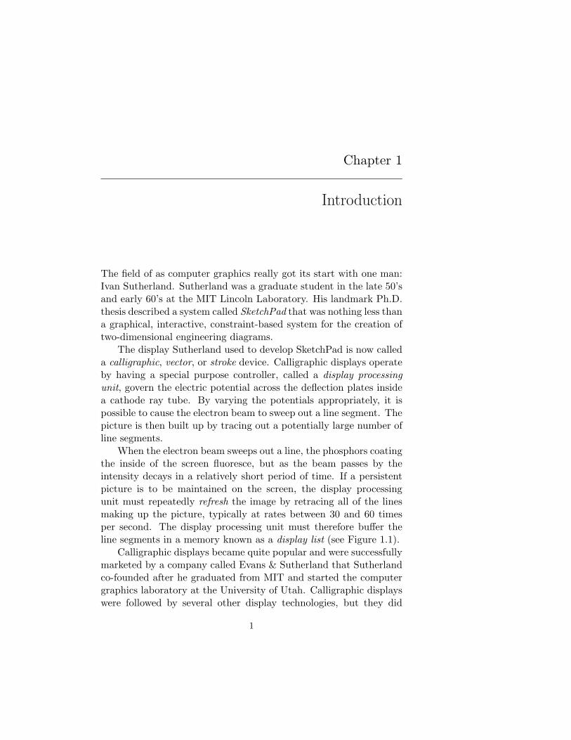
The field of as computer graphics really got its start with one man:Ivan Sutherland. Sutherland was a graduate student in the late 50’sand early 60’s at the MIT Lincoln Laboratory. His landmark Ph.D.thesis described a system called SketchPad that was nothing less thana graphical, interactive, constraint-based system for the creation oftwo-dimensional engineering diagrams.
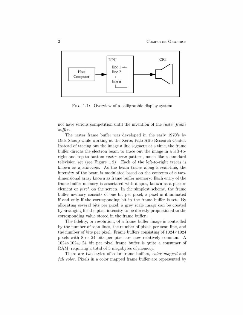
The display Sutherland used to develop SketchPad is now calleda calligraphic, vector, or stroke device. Calligraphic displays operateby having a special purpose controller, called a display processingunit, govern the electric potential across the deflection plates insidea cathode ray tube. By varying the potentials appropriately, it ispossible to cause the electron beam to sweep out a line segment. Thepicture is then built up by tracing out a potentially large number ofline segments.
When the electron beam sweeps out a line, the phosphors coatingthe inside of the screen fluoresce, but as the beam passes by theintensity decays in a relatively short period of time. If a persistentpicture is to be maintained on the screen, the display processingunit must repeatedly refresh the image by retracing all of the linesmaking up the picture, typically at rates between 30 and 60 timesper second. The display processing unit must therefore buffer theline segments in a memory known as a display list (see Figure 1.1).
Calligraphic displays became quite popular and were successfullymarketed by a company called Evans & Sutherland that Sutherlandco-founded after he graduated from MIT and started the computergraphics laboratory at the University of Utah. Calligraphic displayswere followed by several other display technologies, but they did
1
Host Computer
DPU
line 1line 2
:line n
CRT
2 Computer Graphics
Fig. 1.1: Overview of a calligraphic display system
not have serious competition until the invention of the raster framebuffer.
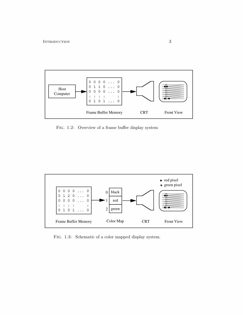
The raster frame buffer was developed in the early 1970’s byDick Shoup while working at the Xerox Palo Alto Research Center.Instead of tracing out the image a line segment at a time, the framebuffer directs the electron beam to trace out the image in a left-to-right and top-to-bottom raster scan pattern, much like a standardtelevision set (see Figure 1.2). Each of the left-to-right traces isknown as a scan-line. As the beam traces along a scan-line, theintensity of the beam is modulated based on the contents of a two-dimensional array known as frame buffer memory. Each entry of theframe buffer memory is associated with a spot, known as a pictureelement or pixel, on the screen. In the simplest scheme, the framebuffer memory consists of one bit per pixel; a pixel is illuminatedif and only if the corresponding bit in the frame buffer is set. Byallocating several bits per pixel, a grey scale image can be createdby arranging for the pixel intensity to be directly proportional to thecorresponding value stored in the frame buffer.
The fidelity, or resolution, of a frame buffer image is controlledby the number of scan-lines, the number of pixels per scan-line, andthe number of bits per pixel. Frame buffers consisting of 1024×1024pixels with 8 or 24 bits per pixel are now relatively common. A1024×1024, 24 bit per pixel frame buffer is quite a consumer ofRAM, requiring a total of 3 megabytes of memory.
There are two styles of color frame buffers, color mapped andfull color. Pixels in a color mapped frame buffer are represented by
Host Computer
CRT
0 0 0 0 ... 00 1 1 0 ... 00 0 0 0 ... 0: : : : :0 1 0 1 ... 0
Frame Buffer Memory Front View
CRT
0 0 0 0 ... 00 1 2 0 ... 00 0 0 0 ... 0: : : : :0 1 0 1 ... 0
Frame Buffer Memory Front View
black
red
green
0
1
2
Color Map
red pixelgreen pixel
Introduction 3
Fig. 1.2: Overview of a frame buffer display system
Fig. 1.3: Schematic of a color mapped display system.

4 Computer Graphics
an 8 to 12 bit color index. The color indices are turned into colorsusing a lookup table called a color map, as indicated in Figure 1.3.Referring to Figure 1.3, color index number 2, for example, is mappedinto the color green. To understand exactly what is stored in eachof the entries of the color map, we must look more closely at howcolor video monitors operate. Whereas monochrome monitors accepta single intensity signal or channel, a color video monitor requiresthree channels: one for red, one for green, and one for blue. Eachcolor map entry i therefore stores three values to indicate the red,green, and blue intensities to associate with color index i. Eachof the channel intensities is typically designated with 8 to 16 bitintegers. A color map for turning 8 bits per pixel values into three8 bit intensity channels would require 28 ∗ 3 ∗ 1 = 768 bytes, andwould allow color images consisting of up to 256 colors chosen froma pallete of 224 possible colors.
The creation of high-quality smooth shaded color images requiresmany more than 256 colors. These images can only be accuratelydisplayed on a full color frame buffer where at least 24 bits perpixel are available. Notice that color maps as described above wouldbe prohibitively expensive in that the color map would be muchlarger than the frame buffer memory itself. Full color frame bufferstherefore essentially do away with the color map, treating the 24bits stored at each pixel as being composed of three 8 bit quantitiesindicating the intensities of each of the three color channels.
Higher quality full color frame buffers typically provide threelookup tables, one for each of the three color channels, that can beused to achieve certain special effects or to correct for non-linearitiesin the display. A non-linearity that is always present in displaysystems is caused by the behavior of the phosphors. The intensityI of a phosphor is proportional to δγ , where δ is the number ofelectrons striking the phosphor per unit time and γ is a constantthat depends on a number of factors including the type of phosphorand the way it was deposited on the surface of the CRT. In a framebuffer display system, δ is in turn proportional to the value associatedwith a pixel, implying that the value of a pixel is non-linearly relatedto the intensity of the spot. The non-linearities can be compensatedfor by the lookup tables by storing at index i a value proportional
to i1γ . Working through the chain of proportionalities it is easy
to show that this ensures that the pixel value i is linearly related

Introduction 5
to the intensity. This process has come to be known as gammacorrection [5]. Since the value of γ must be known to initialize thelookup tables, true gamma correction requires that the value of γ bemeasured experimentally for each monitor.
Exercises
1. A spectraphotometer is a device that can accurately measurethe intensity of a source of illumination. Describe a procedurefor using a spectraphotometer to determine what values tostore in a full color frame buffer’s lookup tables to achievegamma corrected images.

6 Computer Graphics
Chapter 2
Two-Dimensional Raster Algorithms
In this and subsequent chapters we will build up techniques forcreating color images of complex three-dimensional environmentsusing full color frame buffers. The basic problem to be addressedmay roughly be stated as:
Given: A mathematical description of a two or three-dimensional “scene” and a viewing position.
Find: A value for each pixel in the frame buffer suchthat the image on the screen is a reasonably accuratepicture of what an imaginary viewer would see.
There are, admittedly, a number of ill-defined terms in the abovestatement, but each of these ideas will be made much more preciseas we go along.
The first step in our study of raster graphics is to developa variety of basic raster algorithms. The most primitive rasteroperation is the drawing of a dot, i.e., setting a pixel to someparticular value. For the next several chapters we will consider onlythe construction of monochrome images. We assume that pixels canbe set using a primitive operation:
fb writePixel( x, y : integer; c : Color)
where, for now, the legal values for c are assumed to be WHITEor BLACK. The x and y parameters to fb writePixel() indicate (ie,address) which pixel is to be modified. Unfortunately, addressingconventions differ from frame buffer to frame buffer. For instance,
7

(x1,y1)
(x2,y2)
8 Computer Graphics
Fig. 2.1: To scan-convert the line segment connecting (x1, y1) to(x2, y2), the intermediate pixels must be identified and illuminated.Grid lines denote pixel centers.
pixels on an X window display are addressed so that the upper leftcorner of the screen corresponds to (x, y) = (0, 0), with x increasingto the right and y increasing downward. Other devices adopt theconvention that (0, 0) is the lower left corner, with x increasing tothe right and y increasing upward. In this way each frame bufferdefines its own device coordinate system that associates (x, y) to pixellocations. We say that x and y as above are device coordinates.
2.1. Scan-converting Line Segments
The process of painting or rendering a geometric entity such as apoint, line, or circle into a frame buffer is called scan-conversion.Above we assumed that the scan-conversion of points was imple-mented by the primitive operation fb writePixel(). In this sectionwe examine the scan-conversion of the simplest non-trivial geomet-ric entity, the line segment. Specifically, we consider the followingproblem:
Given: Two pixel locations (x1, y1) and (x2, y2) in devicecoordinates.
Find: The intermediate pixels to illuminate to representthe line segment connecting (x1, y1) to (x2, y2) as indi-cated in Figure 2.1.
We will solve this problem by beginning with a more or lessobvious method, then refine the method until we derive an algorithm
Raster Algorithms 9
that strikes a sensible balance between speed, accuracy, and easeof implementation. In the remainder of this section, we assumethat device coordinates are such that x increases to the right andy increases upward.
We should first lay down a set of properties we would like oursolutions to possess. Although some of the following propertiesseem obvious enough to ignore, we shall see apparently acceptablealgorithms that fail to possess them.
Properties:1. Lines should appear as straight as possible.
2. Lines should terminate exactly at (x1, y1) and (x2, y2).
3. Lines should have relatively constant intensities.
4. The intensity of a line should be independent of slope.
5. The algorithm should be relatively efficient since line drawingis in the inner loop of many applications.
2.1.1. The Line Equation Algorithm The first algorithm forscan-converting the line segment (x1, y1), (x2, y2) might be called the“Line Equation Algorithm” since it is based on the familiar equationy = mx + b for lines, where m is the slope and b is the y intercept.Figure 2.2 presents a pseudo-code statement of the algorithm.
Although this algorithm is intuitive, it fails to possess several ofthe properties listed above. Notice that only one pixel is illuminatedin each pixel column. This means that if L1 and L2 are two linesegments of equal length emanating from (x1, y1), with the slope ofL1 greater than the slope of L2, then fewer pixels will be illuminatedfor L1 than for L2. This violates property 4 since it implies that theperceived intensity of the scan-converted line depends on the slope.Passing to the limit of infinite slope (i.e., a vertical line) we discovera more serious problem with the algorithm: it causes an arithmeticexception (a stoic term for “crashes”) when it attempts to divide by(x2 − x1), which is, of course, zero for vertical lines.
2.1.2. The Digital Differential Analyzer The problems en-countered with the Line Equation Algorithm can be partially reme-died by noting that there is a symmetry in the problem that is not

10 Computer Graphics
LineEquationAlgorithm( x1, y1, x2, y2 : integer; c : Color)begin
m,b: real;x,dx: integer;
m := (y2-y1)/(x2-x1);b := y1-m*x1;if (x2 - x1) > 0 then
dx := 1.0;else
dx := -1.0;endif;
for x := x1 to x2 step dx doy := m*x + b;fb writePixel( x, Round(y), c);
endfor;end
Fig. 2.2: A straightforward line drawing algorithm based on theline equation y = mx + b.
Raster Algorithms 11
reflected in the algorithm. In the original problem statement forscan-converting lines, the x and y coordinates play completely sym-metric roles, whereas the Line Equation Algorithm breaks this sym-metry by always computing y as a function of x. The algorithm cantherefore be improved by modifying it to interchange the roles of xand y if |y2−y1| > |x2−x1|. The algorithm can be further improvedto reduce the number of floating point computations required in theinner loop. The key is to exploit the fact that the y value yi+1 neededfor the i+1st iteration can be computed incrementally from yi. Therelation
xi+1 = xi + 1,
implies that
yi+1 = m(xi + 1) + b = yi + m,
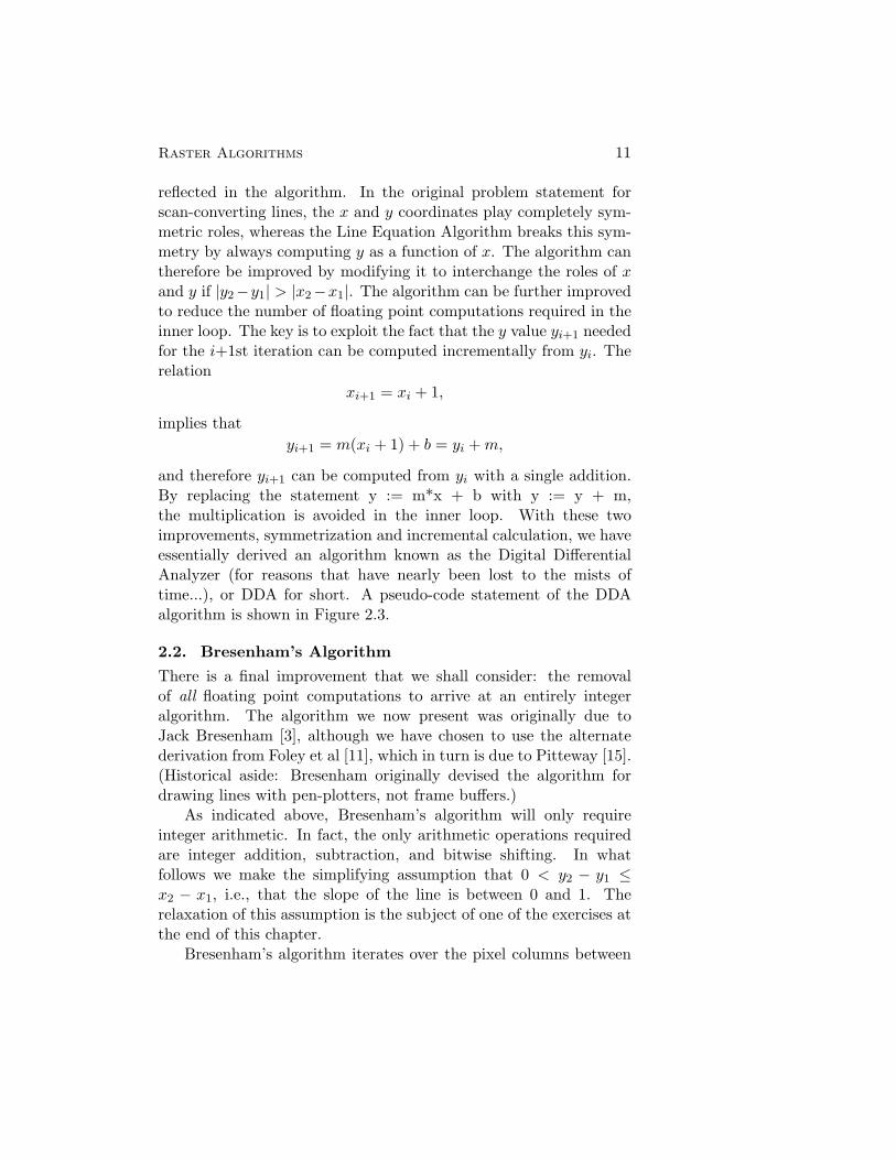
and therefore yi+1 can be computed from yi with a single addition.By replacing the statement y := m*x + b with y := y + m,the multiplication is avoided in the inner loop. With these twoimprovements, symmetrization and incremental calculation, we haveessentially derived an algorithm known as the Digital DifferentialAnalyzer (for reasons that have nearly been lost to the mists oftime...), or DDA for short. A pseudo-code statement of the DDAalgorithm is shown in Figure 2.3.
2.2. Bresenham’s Algorithm
There is a final improvement that we shall consider: the removalof all floating point computations to arrive at an entirely integeralgorithm. The algorithm we now present was originally due toJack Bresenham [3], although we have chosen to use the alternatederivation from Foley et al [11], which in turn is due to Pitteway [15].(Historical aside: Bresenham originally devised the algorithm fordrawing lines with pen-plotters, not frame buffers.)
As indicated above, Bresenham’s algorithm will only requireinteger arithmetic. In fact, the only arithmetic operations requiredare integer addition, subtraction, and bitwise shifting. In whatfollows we make the simplifying assumption that 0 < y2 − y1 ≤x2 − x1, i.e., that the slope of the line is between 0 and 1. Therelaxation of this assumption is the subject of one of the exercises atthe end of this chapter.
Bresenham’s algorithm iterates over the pixel columns between
12 Computer Graphics
DDA( x1, y1, x2, y2: integer; c: Color)begin
length, dx, dy, i: integer;x, y, xincr, yincr: real;
dx := x2 - x1;dy := y2 - y1;length := max( |dx|, |dy|);
{ Either xincr or yincr has magnitude 1. }xincr := dx/length;yincr := dy/length;
x := x1; y := y1;for i := 1 to length+1 do
fb writePixel( Round(x), Round(y), c);x:= x + xincr;y:= y + yincr;
endfor;end
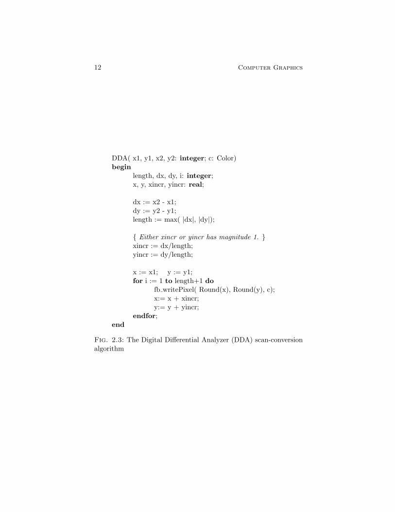
Fig. 2.3: The Digital Differential Analyzer (DDA) scan-conversionalgorithm
Pi-1 Ei
NEi
Mi
Raster Algorithms 13
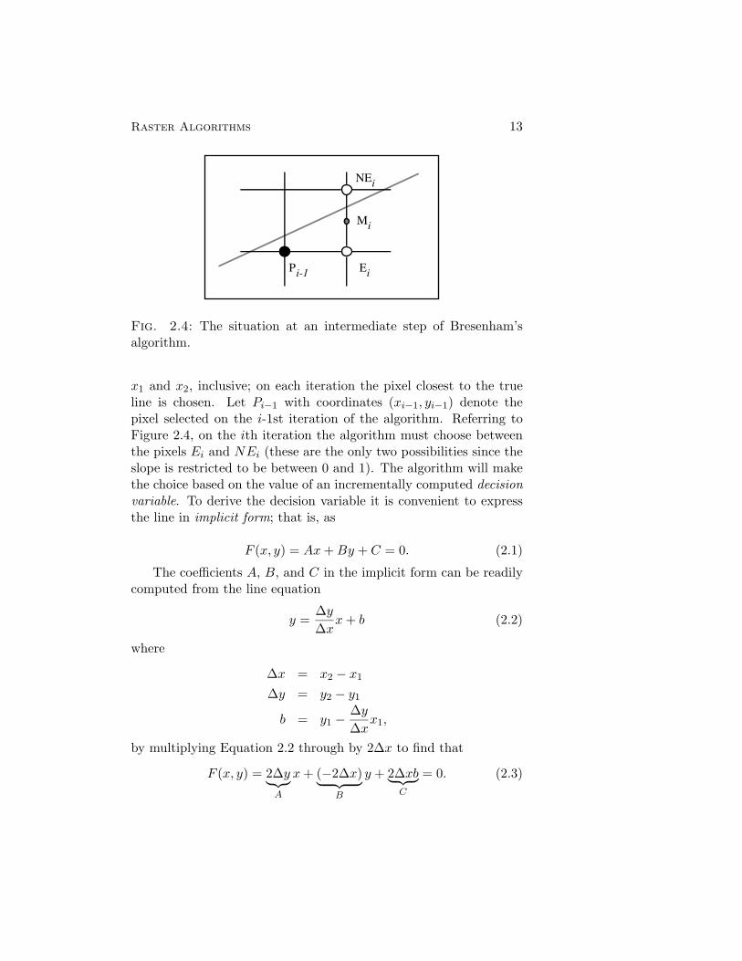
Fig. 2.4: The situation at an intermediate step of Bresenham’salgorithm.
x1 and x2, inclusive; on each iteration the pixel closest to the trueline is chosen. Let Pi−1 with coordinates (xi−1, yi−1) denote thepixel selected on the i-1st iteration of the algorithm. Referring toFigure 2.4, on the ith iteration the algorithm must choose betweenthe pixels Ei and NEi (these are the only two possibilities since theslope is restricted to be between 0 and 1). The algorithm will makethe choice based on the value of an incrementally computed decisionvariable. To derive the decision variable it is convenient to expressthe line in implicit form; that is, as
F (x, y) = Ax + By + C = 0. (2.1)
The coefficients A, B, and C in the implicit form can be readilycomputed from the line equation
y =∆y
∆xx + b (2.2)
where
∆x = x2 − x1
∆y = y2 − y1
b = y1 −∆y
∆xx1,
by multiplying Equation 2.2 through by 2∆x to find that
F (x, y) = 2∆y︸︷︷︸A
x + (−2∆x)︸ ︷︷ ︸B
y + 2∆xb︸ ︷︷ ︸C
= 0. (2.3)
14 Computer Graphics
The justification for multiplying by 2∆x instead of ∆x will becomeapparent shortly. From Equation 2.3 we observe that
1. If F (x, y) < 0, the point (x, y) is above the line.
2. If F (x, y) > 0, the point (x, y) is below the line.
3. A, B, and C are integers.
Observations 1 and 2 imply that if Mi denotes the midpointbetween Ei and NEi, and if F (Mi) < 0, then Pi := Ei (that is, Ei
should be chosen on the ith iteration); otherwise, Pi := NEi. (Thinkabout what should be done if F (Mi) = 0.)
The number di = F (Mi) is the decision variable we were seeking.The convenient aspect of this particular choice of the decisionvariable is that it can be computed incrementally using only integerarithmetic. If Ei is chosen on the ith iteration, then
di+1 = F (xi−1 + 2, yi−1 +1
2)
= di + A,
and if NEi is chosen on the ith iteration, a similar analysis showsthat
di+1 = di + A + B.
About the only remaining detail is to discover how to initialize thedecision variable. It is not difficult to show that
d1 = A +B
2.
The seemingly extraneous factor of two that was introduced into thedefinitions of A, B, and C was chosen precisely so that d1 would bean integer. A pseudo-code statement of the complete algorithm isgiven in Figure 2.5.
2.3. The Device Abstract Data Type
We will eventually be developing relatively sophisticated applicationprograms that read in geometric data, process them in various ways,and finally scan-convert them to create an image. As our formalismcurrently stands, application programs must know the specifics of thedevice coordinate systems for each of the devices they are to output

Raster Algorithms 15
Bresenham( x1, y1, x2, y2 : integer; c : Color){ Draw the line segment from (x1,y1) to (x2,y2) assuming that the }{ slope of the line is between 0 and 1 }begin
d, dx, dy, x, y : integer;incrE : integer; { Amount to add when E chosen }incrNE : integer; { Amount to add when NE chosen }
{ Compute loop invariant quantities }dx := x2 - x1;dy := y2 - y1;incrE := dy << 1; { << 1 means left shift by 1 bit }
{ Initialize incremental quantities }d := incrE - dx;incrNE := d - dx;x := x1; y := y1;fb writePixel( x, y, c);
{ Scan-convert the line segment }while (x < x2) do
x := x + 1;if (d < 0) then
{ Choose E }d := d + incrE;
else{ Choose NE }d := d + incrNE;y := y + 1;
endiffb writePixel( x, y, c);
endwhile;end;
Fig. 2.5: Bresenham’s algorithm for scan-converting lines whoseslope is between 0 and 1.
16 Computer Graphics
to. Software engineering practices suggest that this informationshould be encapsulated to define an abstract data type (ADT) thatmodels an idealized display device. The definition of the deviceADT should abstract out as many of the details of specific devicesas possible. Abstraction of detail is, however, in tension with thedesire to take advantage of special hardware features of many modernframe buffers. For example, some graphics display systems currentlyprovide hardware support for bit blit, the rapid copying of blocks ofpixel values to and from the frame buffer memory. The designer ofa portable device ADT may therefore be faced with difficult choiceswhen deciding which high level operations to include and which toexclude.
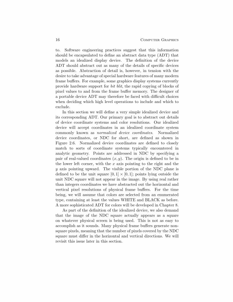
In this section we will define a very simple idealized device andits corresponding ADT. Our primary goal is to abstract out detailsof device coordinate systems and color resolutions. Our idealizeddevice will accept coordinates in an idealized coordinate systemcommonly known as normalized device coordinates. Normalizeddevice coordinates, or NDC for short, are defined as shown inFigure 2.6. Normalized device coordinates are defined to closelymatch to sorts of coordinate systems typically encountered inanalytic geometry. Points are addressed in NDC by specifying apair of real-valued coordinates (x, y). The origin is defined to be inthe lower left corner, with the x axis pointing to the right and they axis pointing upward. The visible portion of the NDC plane isdefined to be the unit square [0, 1] × [0, 1]; points lying outside theunit NDC square will not appear in the image. By using real ratherthan integers coordinates we have abstracted out the horizontal andvertical pixel resolutions of physical frame buffers. For the timebeing, we will assume that colors are selected from an enumeratedtype, containing at least the values WHITE and BLACK as before.A more sophisticated ADT for colors will be developed in Chapter 8.
As part of the definition of the idealized device, we also demandthat the image of the NDC square actually appears as a squareon whatever physical screen is being used. This is not as easy toaccomplish as it sounds. Many physical frame buffers generate non-square pixels, meaning that the number of pixels covered by the NDCsquare must differ in the horizontal and vertical directions. We willrevisit this issue later in this section.
1
1
x
y
Visible Portion of
NDC
Raster Algorithms 17
Fig. 2.6: Normalized device coordinates
Operations on the idealized device include:1
• DeviceDrawDot( x, y : real; c : Color)Draw a dot at the point (x, y) in the color specific by c.
• DeviceDrawLine( x1, y1, x2, y2: real; c : Color)Draw a line from (x1, y2) to (x2, y2) in the color specified by c.
• DeviceDrawText( x, y : real; str : string; c : Color)Draw the string str starting at the point (x, y). (A moresophisticated device ADT would include control over the sizeand perhaps the font the string is to be drawn in.)
An implementation of device ADT is a body of software, gener-ally called a device driver, that maps the abstractions of the idealizeddevice onto a concrete frame buffer. The device driver therefore en-capsulates all device dependent information, making it easy to portapplications from one device to another.
One of the principal responsibilities of a device driver is to trans-form normalized device coordinates (nx, ny) into device coordinates(dx, dy) appropriate for the frame buffer at hand. A pair of transfor-mations ToDevx : nx �→ dx and ToDevy : ny �→ dy that operate onx and y coordinates, respectively, can be used for this purpose. Asa specific example of the development of such coordinate transfor-mations, suppose the device coordinates are as shown in Figure 2.7,
1All coordinates are specified in NDC.

(0,0) (XRES,0)
(0,YRES)
18 Computer Graphics
Fig. 2.7: A typical physical device coordinate system.
where the lower left corner of the screen corresponds to (0, 0), thelower right corner to (XRES , 0), the upper left corner to (0, YRES),and the upper right corner to (XRES , YRES). The integers XRES
and YRES refer to number of pixels on the screen in the horizontaland vertical directions. Suppose further that the physical screen iswider than it is tall (a ratio of 4 to 3 is common, but by no meansuniversal).
We shall construct the transformations ToDevx() and ToDevy()so that the image of the NDC unit square will overlay the largestcentral square portion of the screen, as indicated in Figure 2.8.Denote by x0 and x1 the x device coordinates of the left and rightedges of the image of the NDC unit square. In practice these numbersmust be determined by physically measuring the screen (who sayscomputer science isn’t a physical science?). The function ToDevx()is therefore subject to two constraints:
1. ToDevx(0) = x0.
2. ToDevx(1) = x1.
If ToDevx() is chosen to be a linear function, it is completelydetermined by these two conditions:
ToDevx(nx) = (1 − nx) x0 + nx x1. (2.4)
A similar process for ToDevy() shows that
ToDevy(ny) = ny YRES . (2.5)

0 XRESx0 x1
Image of NDC square centered on the frame buffer
Raster Algorithms 19
Fig. 2.8: The NDC square is mapped to the largest central squareon the physical screen.
Given procedures to compute ToDevx() and ToDevy(), an imple-mentation of DeviceDrawLine() could simply transform x1, y1, x2, y2
to device coordinates, then use Bresenham’s algorithm to scan-convert the line.
2.4. The Simple Graphics Package
In this section we begin the development of a layer of graphicssoftware designed to provide convenient, general facilities to higherlevel application programs. We shall refer to this set of routines asthe Simple Graphics Package, or SGP. SGP will serve as a mediatorbetween the device ADT on the low-level side, and the applicationprogram on the high-level side. To motivate the initial developmentof SGP, in the next several sections we consider the constructionof a simple two-dimensional data plotting program. A good dealof the rest of the text is devoted to extending SGP to handle thespecification and viewing of three-dimensional smooth shaded colorimages.
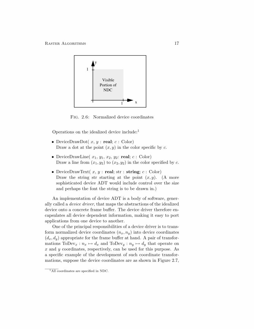
2.4.1. Two-Dimensional Windowing and ViewportingConsider a program that reads in two dimensional data points andcreates images such as the one shown in Figure 2.9 that plots yearlyrainfall (in feet for Seattle, in inches for California). In this examplethe independent variable is the year and the dependent variable isthe rainfall. Since the data points lie outside the unit square, we
88
2.0
3.0
4.0
89 90 91
Year
Rain fall
20 Computer Graphics
Fig. 2.9: A sample plot.
must first transform them to points in the unit square before usingroutines such as DeviceDrawLine().
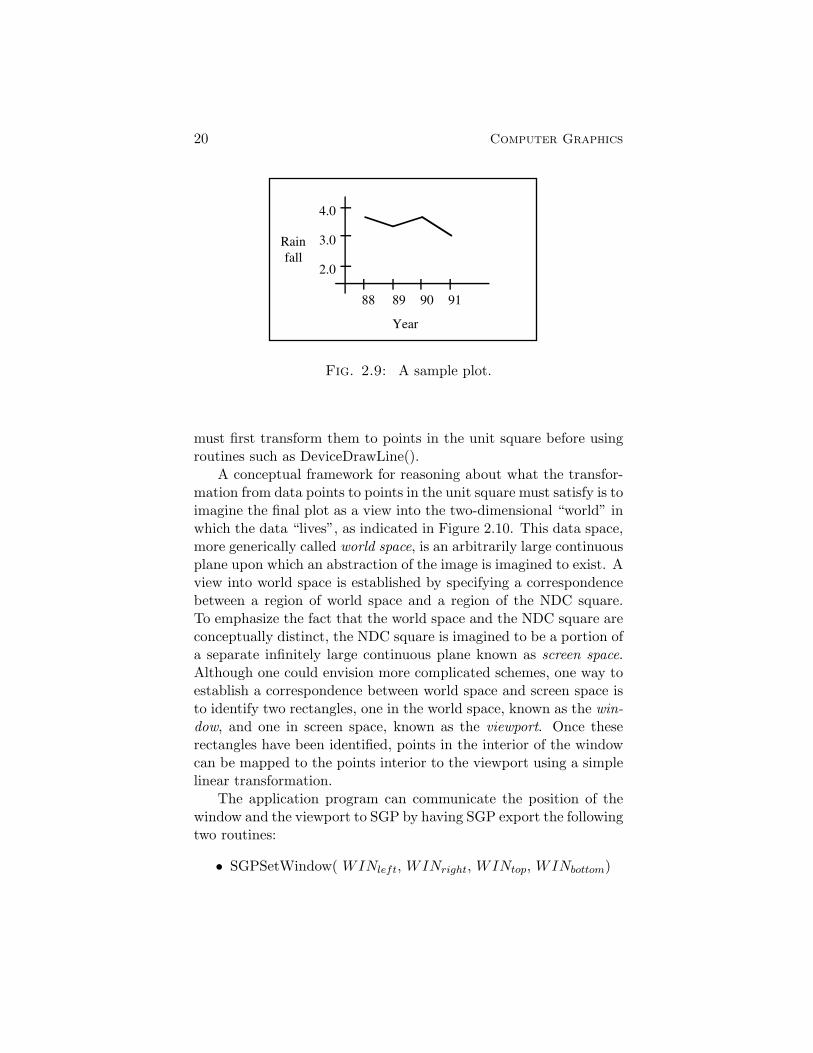
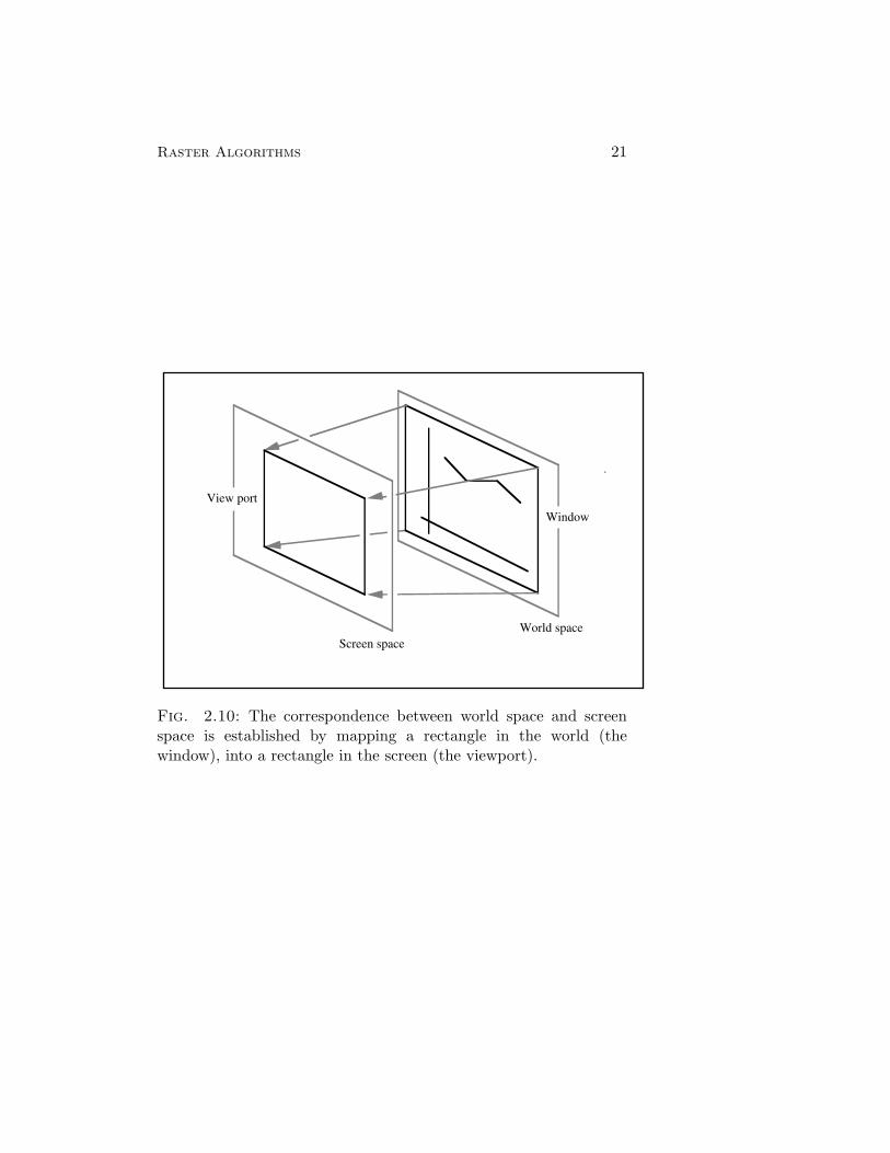
A conceptual framework for reasoning about what the transfor-mation from data points to points in the unit square must satisfy is toimagine the final plot as a view into the two-dimensional “world” inwhich the data “lives”, as indicated in Figure 2.10. This data space,more generically called world space, is an arbitrarily large continuousplane upon which an abstraction of the image is imagined to exist. Aview into world space is established by specifying a correspondencebetween a region of world space and a region of the NDC square.To emphasize the fact that the world space and the NDC square areconceptually distinct, the NDC square is imagined to be a portion ofa separate infinitely large continuous plane known as screen space.Although one could envision more complicated schemes, one way toestablish a correspondence between world space and screen space isto identify two rectangles, one in the world space, known as the win-dow, and one in screen space, known as the viewport. Once theserectangles have been identified, points in the interior of the windowcan be mapped to the points interior to the viewport using a simplelinear transformation.
The application program can communicate the position of thewindow and the viewport to SGP by having SGP export the followingtwo routines:
• SGPSetWindow( WINleft, WINright, WINtop, WINbottom)
Screen spaceWorld space
View port
Window
Raster Algorithms 21
Fig. 2.10: The correspondence between world space and screenspace is established by mapping a rectangle in the world (thewindow), into a rectangle in the screen (the viewport).

22 Computer Graphics
• SGPSetViewPort( V Pleft, V Pright, V Ptop, V Pbottom)
The arguments to these routines specify the left, right, top and bot-tom extents of the window and viewport, respectively. The param-eters to SGPSetWindow() correspond to coordinates in the worldspace, whereas the parameters to SGPSetViewPort() correspond tocoordinates in screen space. The calls necessary for establishing theconnection indicated in Figure 2.10 might be something like:
SGPSetWindow( 85, 93, 4.5, -4.0)SGPSetViewPort( 0.25, 0.75, 0.75, 0.25)
A point (wx, wy) in world space can be transformed into thecorresponding point (nx, ny) in screen space using a pair of linearfunctions similar to ToDevx() and ToDevy(). Denoting thesefunctions by ToNDCx() and ToNDCy(), it is not difficult to showthat (nx, ny) = (ToNDCx(wx),ToNDCy(wy)) where
ToNDCx(wx) =V Pright − V Pleft
WINright −WINleft(wx −WINleft) + V Pleft
ToNDCy(wy) =V Ptop − V Pbottom
WINtop −WINbottom(wy −WINbottom) + V Pbottom
Having established the correspondence between the world andscreen spaces, SGP can take on the responsibility for automaticallytransforming drawing requests to screen space, allowing the applica-tion program to work more naturally in world coordinates. Specifi-cally, SGP can export the routines
• SGPDrawDot( x, y : real; c : Color)Draw a dot at the world space point (x, y).
• SGPDrawLine( x1, y1, x2, y2 : real; c : Color)Draw the world space line segment from (x1, y1) to (x2, y2).
• SGPDrawText( x, y : real; str : string; c : Color)Draw the string str starting at the world space point (x, y).
These routines are most simply implemented by transforming theworld space points into points in screen space by using ToNDCx()and ToNDCy(), followed by calling the corresponding routine ex-ported by the device ADT.
Raster Algorithms 23
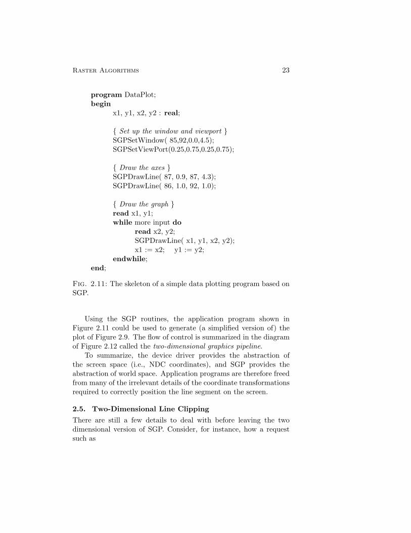
program DataPlot;begin
x1, y1, x2, y2 : real;
{ Set up the window and viewport }SGPSetWindow( 85,92,0.0,4.5);SGPSetViewPort(0.25,0.75,0.25,0.75);
{ Draw the axes }SGPDrawLine( 87, 0.9, 87, 4.3);SGPDrawLine( 86, 1.0, 92, 1.0);
{ Draw the graph }read x1, y1;while more input do
read x2, y2;SGPDrawLine( x1, y1, x2, y2);x1 := x2; y1 := y2;
endwhile;end;
Fig. 2.11: The skeleton of a simple data plotting program based onSGP.
Using the SGP routines, the application program shown inFigure 2.11 could be used to generate (a simplified version of) theplot of Figure 2.9. The flow of control is summarized in the diagramof Figure 2.12 called the two-dimensional graphics pipeline.
To summarize, the device driver provides the abstraction ofthe screen space (i.e., NDC coordinates), and SGP provides theabstraction of world space. Application programs are therefore freedfrom many of the irrelevant details of the coordinate transformationsrequired to correctly position the line segment on the screen.
2.5. Two-Dimensional Line Clipping
There are still a few details to deal with before leaving the twodimensional version of SGP. Consider, for instance, how a requestsuch as

Clip
Windowto
Viewport
Scan-convert
NDC to DC
Application Program
Device
SGP
Device Driver
World Coordinates
Normalized Device Coordinates
Device Coordinates
24 Computer Graphics
Fig. 2.12: The two-dimensional graphics pipeline as typicallyimplemented in software.

Raster Algorithms 25
SGPDrawLine( 91, 3.0, 92, 10.0)2
should be dealt with. The usual action in such a case is to clipthe line segment to the interior of the window. That is, we wishto trim away that part of the line segment that lies outside thewindow, and process the remainder as before. We will examinetwo line clipping algorithms in this section. The first is intendedas a software solution whereas the second is particularly suited toa hardware implementation. A third line clipping algorithm, onethat is easily extended to the clipping of polygons in two and threedimensions, is presented in Section 3.9.
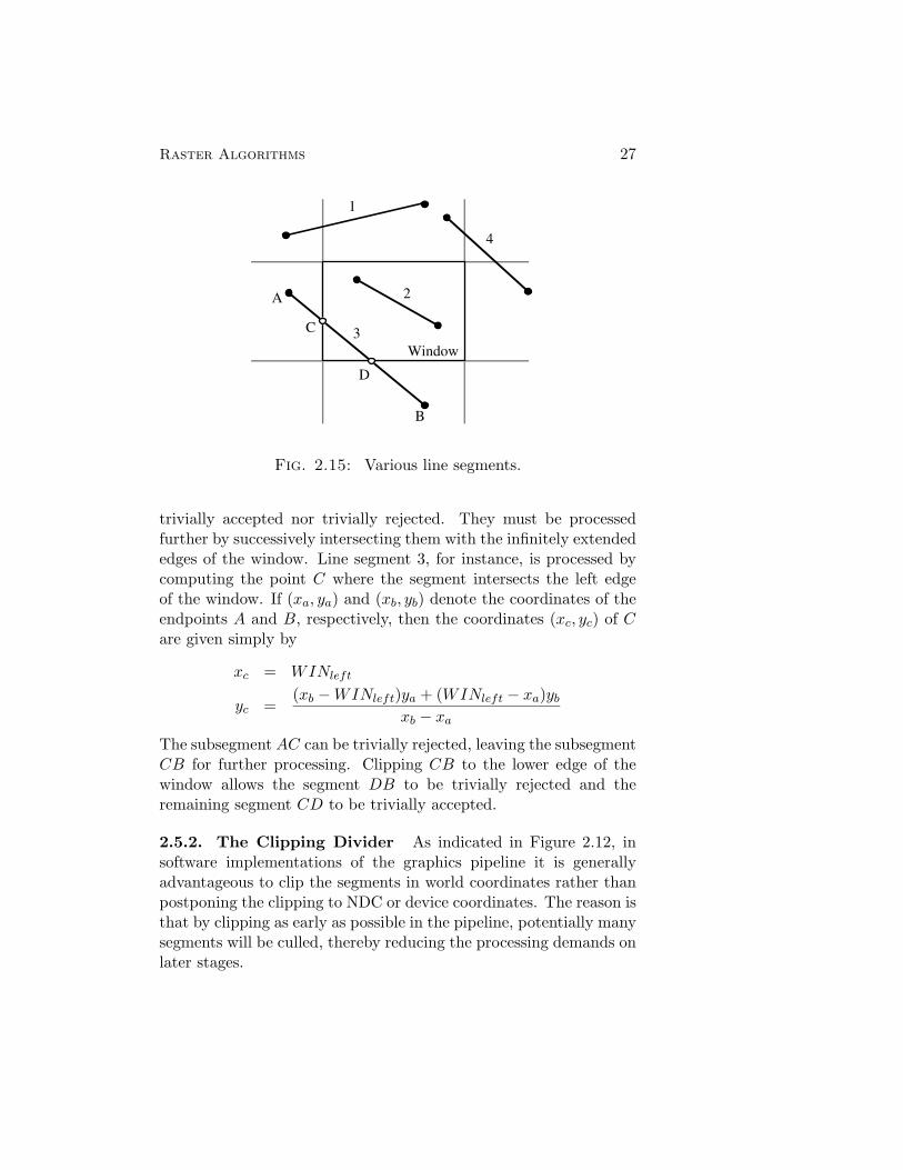
2.5.1. Cohen-Sutherland Line Clipping Cohen and Suther-land developed a particularly efficient method for clipping line seg-ments that is based on a clever classification of the endpoints of thesegment. The Cohen-Sutherland algorithm is constructed to opti-mize the common cases, occurring when the line segment is eitherentirely within the window, or is entirely outside the window. Theclassification is based on the observation that if both endpoints are,say, above the window, then the entire line segment must be abovethe window, and can therefore be trivially rejected. The same sit-uation holds when the endpoints are both left, right, or below thewindow. Each endpoint is therefore characterized by a four-bit vec-tor, called an outcode, that indicates where the endpoint lies relativeto the infinitely extended edges of the window. The meaning of eachof the bits of an outcode is given in Figure 2.13. The outcodes effec-tively divide the world space into nine regions arranged around thewindow as shown in Figure 2.14
If P1 and P2 denote the endpoints of the line to be clipped, thenif the bitwise “anding” of the outcodes of P1 and P2 yields a non-zeroresult, then either both points were left, right, above, or below thewindow. In such a case the entire line segment must be outside thewindow, meaning that the segment can be trivially rejected. Thisis the situation for line segment 1 in Figure 2.15. Line segment 2of Figure 2.15 is entirely within the window. This can be detectedby noting that both endpoints have the outcodes 0000 – such a linesegment is said to be trivially accepted.
The remaining line segments in Figure 2.15 can neither be
2Don’t laugh – in Seattle it could happen.

1001
Window
1000 1010
0001 0000 0010
0101 0100 0110
26 Computer Graphics
Bit Number Meaning if Set
1 Point above window
2 Point below window
3 Point right of window
4 Point left of window
Fig. 2.13: Outcodes assigned to endpoints by the Cohen-Sutherlandalgorithm.
Fig. 2.14: The outcodes partition the world space into nine regionsarranged around the window as shown above.
Window
1
3
2A
B
4
C
D
Raster Algorithms 27
Fig. 2.15: Various line segments.
trivially accepted nor trivially rejected. They must be processedfurther by successively intersecting them with the infinitely extendededges of the window. Line segment 3, for instance, is processed bycomputing the point C where the segment intersects the left edgeof the window. If (xa, ya) and (xb, yb) denote the coordinates of theendpoints A and B, respectively, then the coordinates (xc, yc) of Care given simply by
xc = WINleft
yc =(xb −WINleft)ya + (WINleft − xa)yb
xb − xa
The subsegment AC can be trivially rejected, leaving the subsegmentCB for further processing. Clipping CB to the lower edge of thewindow allows the segment DB to be trivially rejected and theremaining segment CD to be trivially accepted.
2.5.2. The Clipping Divider As indicated in Figure 2.12, insoftware implementations of the graphics pipeline it is generallyadvantageous to clip the segments in world coordinates rather thanpostponing the clipping to NDC or device coordinates. The reason isthat by clipping as early as possible in the pipeline, potentially manysegments will be culled, thereby reducing the processing demands onlater stages.
28 Computer Graphics
The situation is quite different when considering the mapping ofthe graphics pipeline into hardware. In this case it is more convenientto postpone the clipping phase so that it is done in device coordinatesso that integer rather than floating point arithmetic can be used. Theclipping divider [16] is an integer based divide and conquer methodfor clipping line segments in device coordinates. The algorithm teststhe segment being processed for trivial accept and reject conditions.If neither of these cases holds, the midpoint of the segment iscomputed (requiring only shifts and adds), thereby breaking thesegment into two subsegments. Each subsegment is processedrecursively. The clipping divider can easily be implemented usingcurrent VLSI technology, requiring only an integer ALU, a stack,and some simple control logic.
2.6. Windowing and Viewporting Revisited
In preparation for the geometric discussions of the next chapter, letus reexamine the transformation between normalized device coor-dinates and Device Coordinates that was developed in Section 2.3.This transformation, by Equations 2.4 and 2.5, can be written inmatrix form as
(dx dy) = (nx ny)
(x1 − x0 0
0 YRES
)+ (x0 y0).
A trickier form can be used to replace the addition with multiplica-tion of slightly larger matrices:
(dx dy 1) = (nx ny 1)
⎛⎜⎝ x1 − x0 0 0
0 y1 − y0 0x0 y0 1
⎞⎟⎠
︸ ︷︷ ︸N
(2.6)
The transformation between world space and screen space cansimilarly be characterized by the matrix equation
(nx ny 1) = (wx wy 1)
⎛⎜⎝ fx 0 0
0 fy 0tx ty 1
⎞⎟⎠
︸ ︷︷ ︸S
(2.7)

Raster Algorithms 29
where
fx =V Pright − V Pleft
WINright −WINleft
fy =V Ptop − V Pbottom
WINtop −WINbottom
tx = V Pleft − fxWINleft
ty = V Pbottom − fyWINbottom
Combining Equation 2.6 with Equation 2.7 we find that
(dx dy 1) = (wx wy 1)W (2.8)
where the matrix W is the product of S and N.The somewhat mysterious appearance of the third component
of 1 in tuples such as (dx dy 1) and (nx ny 1), and the use of3×3 matrices for two-dimensional transformations will be thoroughlyexplained in the next chapter where we begin in earnest themathematical study of geometry and geometric calculations.
The symbol juggling above shows that the calculations requiredto transform a point from world space into the correspondingpoint in screen space represented in device coordinates can beaccomplished by building and multiplying a carefully chosen set ofmatrices. For this reason computer graphics texts develop geometrictransformations from the point of view of matrix manipulations.We call this a coordinate-based approach since the matrices describeexactly how to combine the coordinates to achieve the (hopefully)desired geometric effect.
While a coordinate-based approach has its merits, not the leastof which is a certain amount of familiarity, it also has some seriousdrawbacks that will be identified in the next chapter. We shalltherefore pursue a coordinate-free treatment that emphasizes thegeometric meaning of an operation instead of the low-level coordinatemanipulations necessary to carry out its computation.
Exercises
1. Generalize Bresenham’s algorithm to accept as input an arbi-trary line segment.

30 Computer Graphics
2. Explain how to speed up Bresenham’s algorithm by roughlya factor of two by exploiting a certain symmetry propertypossessed by the algorithm.
3. Do the DDA algorithm and Bresenham’s algorithm producethe same results? If so, prove it. If not, provide a counterex-ample and characterize the ways in which the pixel patternsdiffer.
4. The line segments created by Bresenham’s algorithm canappear to be rather “jagged”. The jagged appearance of thesegment can be reduced if the frame buffer has more than onebit per pixel used to create grey scale images. The idea is topartially illuminate all the pixels “near” the line so that pixelscloser to the line are brighter. Develop and experiment withsuch a variant of Bresenham’s algorithm, assuming a grey scaleframe buffer that allocates 2b bits per pixel.
5. There is a subtlety in the clipping divider method concerningarithmetic precision. Exactly what precision arithmetic isrequired by the algorithm? Why?
Chapter 3
Coordinate-free Geometric Programming I
3.1. Problems with the Coordinate-based Approach
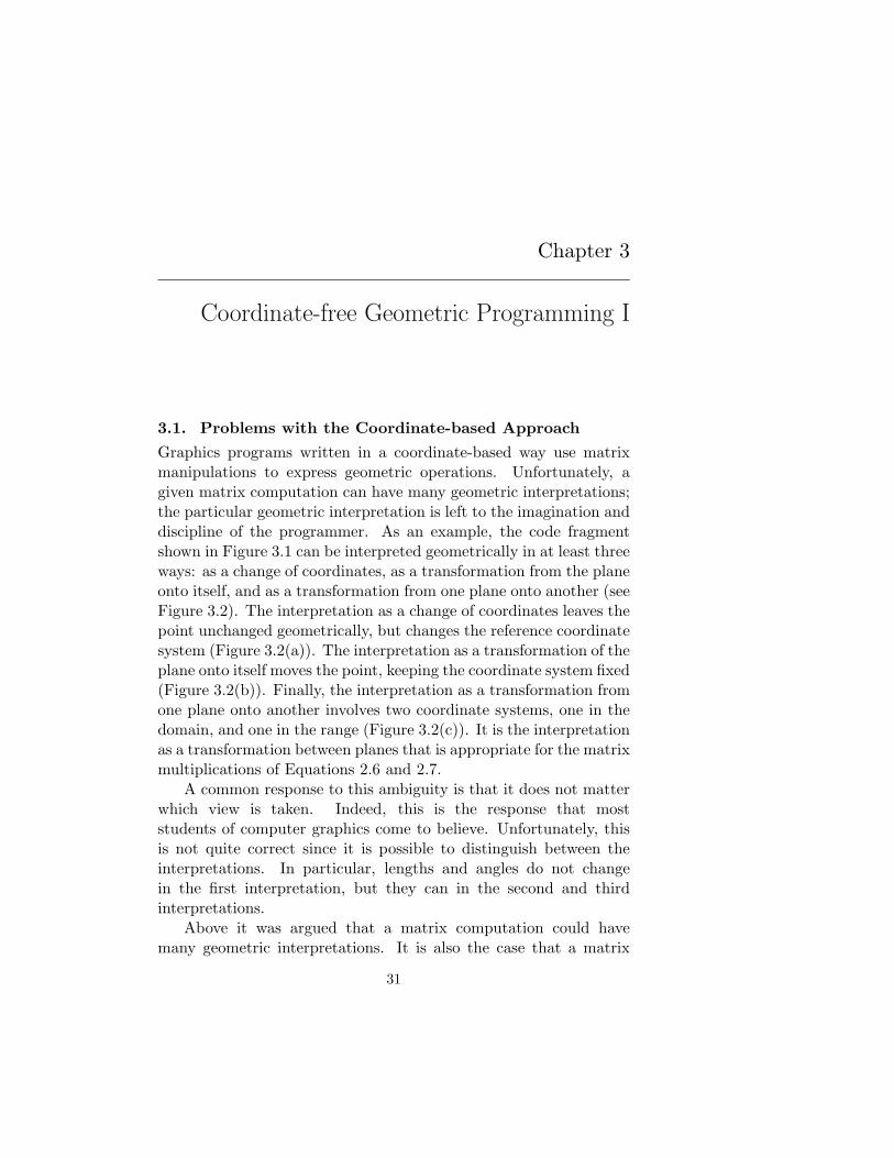
Graphics programs written in a coordinate-based way use matrixmanipulations to express geometric operations. Unfortunately, agiven matrix computation can have many geometric interpretations;the particular geometric interpretation is left to the imagination anddiscipline of the programmer. As an example, the code fragmentshown in Figure 3.1 can be interpreted geometrically in at least threeways: as a change of coordinates, as a transformation from the planeonto itself, and as a transformation from one plane onto another (seeFigure 3.2). The interpretation as a change of coordinates leaves thepoint unchanged geometrically, but changes the reference coordinatesystem (Figure 3.2(a)). The interpretation as a transformation of theplane onto itself moves the point, keeping the coordinate system fixed(Figure 3.2(b)). Finally, the interpretation as a transformation fromone plane onto another involves two coordinate systems, one in thedomain, and one in the range (Figure 3.2(c)). It is the interpretationas a transformation between planes that is appropriate for the matrixmultiplications of Equations 2.6 and 2.7.
A common response to this ambiguity is that it does not matterwhich view is taken. Indeed, this is the response that moststudents of computer graphics come to believe. Unfortunately, thisis not quite correct since it is possible to distinguish between theinterpretations. In particular, lengths and angles do not changein the first interpretation, but they can in the second and thirdinterpretations.
Above it was argued that a matrix computation could havemany geometric interpretations. It is also the case that a matrix
31

P P'P
X
Y = Y'
X'
P
Domain Space Range Space
P'
(a) (b)
(c)
32 Computer Graphics
P ← ( p1 p2 ) ;
T ←(
2 00 1
);
P′ ← P T;
Fig. 3.1: A typical matrix computation.
Fig. 3.2: Three interpretations of the code fragment of Figure 3.1.
Coordinate-free Geometric Programming I 33
computation can have no geometric interpretation. Some errorsare allowed to creep in because there is no explicit representationof coordinate systems or spaces. The programmer is expected tomaintain a clear idea of which coordinate system in which logicalspace (e.g., world coordinates, normalized device coordinates inscreen space, etc.) each point is represented. As a consequence,the burden of coordinate transformations must be borne directly bythe programmer. If extreme care is not taken, it is possible (andin fact common) to perform geometrically meaningless operationssuch as combining two points that reside in different spaces or arerepresented relative to different coordinate systems.
We will address the problems of ambiguity and validity bydeveloping a coordinate-free geometric algebra (i.e., a collection ofgeometric objects together with operations for combining them) thatpromotes geometric reasoning rather than coordinate manipulations.Associated with the algebra will be an ADT that implements theabstractions provided by the algebra. The algebra and ADT areconstructed so that only geometrically meaningful operations arepossible. Moreover, all operations are geometrically unambiguousand their interpretation is clearly reflected by the code.
Although the development of the algebra is done in a coordinate-free way, the ADT must ultimately be implemented using coordi-nates. It is therefore important for the implementor of the ADTto understand how to translate geometric operations into coordi-nate calculations. In an effort to clearly separate the coordinate-freematerial from the coordinate-based material, the coordinate-basedsections have been marked with an asterisk.
3.2. Affine Spaces
Although the geometric ADT will present abstractions based onEuclidean geometry, many of the geometric objects and operationsthat find use in computer graphics and related fields such ascomputer aided geometric design (CAGD) are founded in the moregeneral branch of mathematics known as affine geometry. We havetherefore chosen to develop the affine theory here, then specialize toEuclidean geometry in Section 3.3.
There are many different approaches to affine geometry [8, 10,23]. One approach, first put forth by Weyl [23] (a modern account ofwhich can be found in Dodson and Poston [8] and Flohr and Raith
P
Q
wv
v
34 Computer Graphics
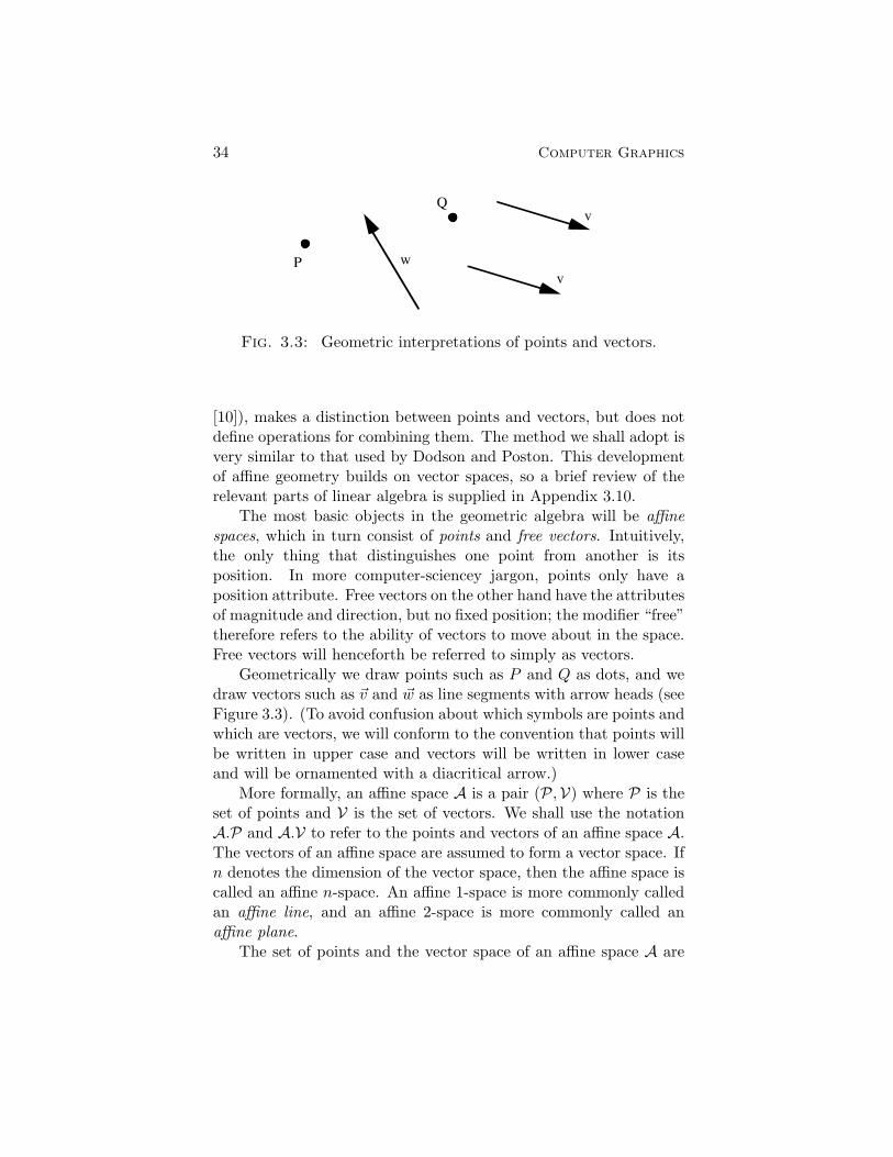
Fig. 3.3: Geometric interpretations of points and vectors.
[10]), makes a distinction between points and vectors, but does notdefine operations for combining them. The method we shall adopt isvery similar to that used by Dodson and Poston. This developmentof affine geometry builds on vector spaces, so a brief review of therelevant parts of linear algebra is supplied in Appendix 3.10.
The most basic objects in the geometric algebra will be affinespaces, which in turn consist of points and free vectors. Intuitively,the only thing that distinguishes one point from another is itsposition. In more computer-sciencey jargon, points only have aposition attribute. Free vectors on the other hand have the attributesof magnitude and direction, but no fixed position; the modifier “free”therefore refers to the ability of vectors to move about in the space.Free vectors will henceforth be referred to simply as vectors.
Geometrically we draw points such as P and Q as dots, and wedraw vectors such as �v and �w as line segments with arrow heads (seeFigure 3.3). (To avoid confusion about which symbols are points andwhich are vectors, we will conform to the convention that points willbe written in upper case and vectors will be written in lower caseand will be ornamented with a diacritical arrow.)
More formally, an affine space A is a pair (P,V) where P is theset of points and V is the set of vectors. We shall use the notationA.P and A.V to refer to the points and vectors of an affine space A.The vectors of an affine space are assumed to form a vector space. Ifn denotes the dimension of the vector space, then the affine space iscalled an affine n-space. An affine 1-space is more commonly calledan affine line, and an affine 2-space is more commonly called anaffine plane.
The set of points and the vector space of an affine space A are

Q
v
Q + v
Coordinate-free Geometric Programming I 35
Fig. 3.4: Addition of points and vectors.
related through the following axioms:(i) Subtraction: There exists an operation of subtraction that
satisfies:
a. For every pair of points P,Q, there is a unique vector �v suchthat �v = P −Q.
b. For every point Q and every vector �v, there is a uniquepoint P such that P −Q = �v.
(ii) The Head-to-Tail Axiom: Every triple of points P,Q and R,satisfies
(P −Q) + (Q−R) = P −R.
Before describing in more detail what the axioms mean geomet-rically, it is convenient to use the them to define the operation ofaddition between points and vectors. Specifically, we define Q + �vto be the unique point P such that P − Q = �v. The geometricinterpretation of addition is shown in Figure 3.4.In terms of the addition operation, axiom (ia) essentially states thatthere are no “points at infinity”, and axiom (ib) guarantees thatthere are no “holes” in the space; together these ensure that if pointQ is fixed, then there is a one-to-one correspondence between vectors(�v) and points (Q + �v). The vector connecting the points Q and Pcan therefore be labeled as P −Q, as shown in Figure 3.5.
The geometric interpretation of axiom (ii), shown in Figure 3.6,indicates that the axiom is actually a statement of the familiar “head-to-tail rule” for vector addition, stated in terms of points ratherthan vectors. (Recall from elementary vector analysis that the vectoraddition �v+ �w can be constructed geometrically by aligning the head

Q
P-Q
P
Q
P-Q
P
R
Q-R
P-R
36 Computer Graphics
Fig. 3.5: Subtraction of points.
Fig. 3.6: The head-to-tail axiom.
of �v with the tail of �w. The sum is then the vector from the tail of�v to the head of �w.)
Example 1. Examples of affine spaces abound. For instance, ifyou believe that time is infinite, then the time line is an exampleof a (one-dimensional) affine space. The points of the affine spacecorrespond to dates, and the vectors of the affine space correspond tonumbers of days. A date (a point) minus another date is a number ofdays (a vector). Thus, subtraction of points makes sense as a vector.The other axioms can also be shown to hold.
The theory of polynomials can be used as the source of anotherexample of an affine space. Let the set of vectors be the setof homogeneous cubic polynomials (a polynomial is said to behomogeneous if its constant coefficient is zero). The set of pointscan then be taken to be the set of cubic polynomials whose constantterm is 1. It is a simple matter to show that the axioms hold when

Coordinate-free Geometric Programming I 37
standard polynomial addition and subtraction are used to add pointsto vectors and to subtract points. The dimension of this affine spaceis 3 since that is the dimension of the space of homogeneous cubicpolynomials.
Several simple deductions can be made from the head-to-tailaxiom. By setting Q = R, we find that (P −Q) + (Q−Q) = P −Q,which implies that Q − Q must be the zero vector �0 since addingit to P − Q results in P − Q. By setting P = R, we see that(R − Q) + (Q − R) = �0, implying that R − Q = −(Q − R). Thesefacts, along with several others, are summarized in the followingclaim.
Claim 1. The following identities hold for all points P , Q andR, and all vectors �v and �w.(a) Q−Q = �0.
(b) R−Q = −(Q−R).
(c) �v + (Q−R) = (Q + �v) −R.
(d) Q− (R + �v) = (Q−R) − �v.
(e) P = Q + (P −Q).
(f) (Q + �v) − (R + �w) = (Q−R) + (�v − �w).
Proof: Parts (a) and (b) were proved above. To prove (c), let pointP be defined by �v = P −Q. The head-to-tail axiom then says that�v + (Q−R) = P −R. The proof is completed by substituting Q+�vfor P . Part (d) follows immediately from (c) by multiplying throughby −1. To prove (e), use the definition of addition together with thehead-to-tail axiom to write P in the form P = R+(P−Q)+(Q−R).Now, taking Q = R we find that P = Q+(P−Q)+�0, which completesthe proof since adding the zero vector to the right side has no affect.
The proof of (f) is somewhat more difficult as it requires the twoinvocations of the head-to-tail axiom together with the use of parts

38 Computer Graphics
(a), (c) and (d):
(Q + �v) − (R +�w)= [(Q + �v) −R] + [R− (R + �w)] by head-to-tail axiom= [(Q + �v) −R] + [(R−R) − �w] by part (d)= [(Q + �v) −R] − �w by part (a)= [(Q + �v) −Q] + [Q−R] − �w by head-to-tail axiom= [�v + (Q−Q)] + [Q−R] − �w by part (c)= (Q−R) + (�v − �w) by part (a)
�
Thus far, the objects in the algebra are space, point, vector, andscalar, and the operations are
vector + vector �→ vector
scalar ∗ vector �→ vector
point − point �→ vector
point + vector �→ point.
For each object in the algebra there should be a correspondingdata type in the ADT, and for each operation in the algebra thereshould be a corresponding procedure. We shall refer to the datatypes as Space, Point, Vector, and Scalar. The Vector and Pointtypes can be tagged with the space in which they reside, makingpossible a wide range of geometric type checking. The procedures ofthe ADT thus far can be summarized as:
• Space ← SCreate( name:string, dim:integer)Return an affine space of dimension dim. The name of thespace is used for debugging purposes. Any number of spacescan be dynamically created.
• Vector ← VVAdd( v, w : Vector)Return the vector sum of v and w. An error is signaled if vand w reside in different spaces.
• Vector ← SVMult( s : Scalar; v : Vector)Return the vector v scaled by s.
• Vector ← PPDiff( p1, p2 : Point)Return the vector p1-p2. An error is signaled if p1 and p2reside in different spaces.
Q1
Q2
Q
α:
1-α
Coordinate-free Geometric Programming I 39
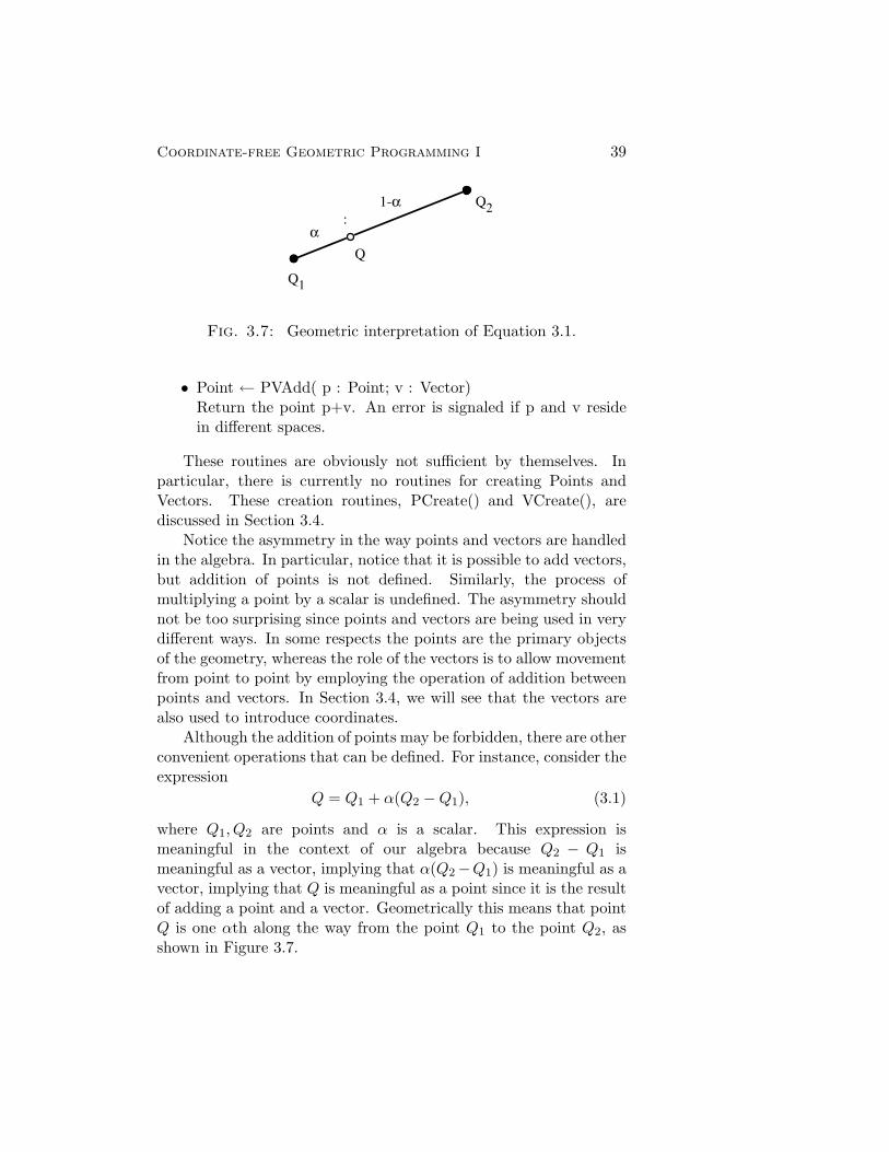
Fig. 3.7: Geometric interpretation of Equation 3.1.
• Point ← PVAdd( p : Point; v : Vector)Return the point p+v. An error is signaled if p and v residein different spaces.
These routines are obviously not sufficient by themselves. Inparticular, there is currently no routines for creating Points andVectors. These creation routines, PCreate() and VCreate(), arediscussed in Section 3.4.
Notice the asymmetry in the way points and vectors are handledin the algebra. In particular, notice that it is possible to add vectors,but addition of points is not defined. Similarly, the process ofmultiplying a point by a scalar is undefined. The asymmetry shouldnot be too surprising since points and vectors are being used in verydifferent ways. In some respects the points are the primary objectsof the geometry, whereas the role of the vectors is to allow movementfrom point to point by employing the operation of addition betweenpoints and vectors. In Section 3.4, we will see that the vectors arealso used to introduce coordinates.
Although the addition of points may be forbidden, there are otherconvenient operations that can be defined. For instance, consider theexpression
Q = Q1 + α(Q2 −Q1), (3.1)
where Q1, Q2 are points and α is a scalar. This expression ismeaningful in the context of our algebra because Q2 − Q1 ismeaningful as a vector, implying that α(Q2 −Q1) is meaningful as avector, implying that Q is meaningful as a point since it is the resultof adding a point and a vector. Geometrically this means that pointQ is one αth along the way from the point Q1 to the point Q2, asshown in Figure 3.7.

40 Computer Graphics
If we forget for a moment that we are dealing with points,vectors, and scalars, we might be tempted to algebraically rearrangeEquation 3.1 into the form
Q = (1 − α)Q1 + αQ2,
or perhaps in the more symmetric form
Q = α1Q1 + α2Q2, α1 + α2 = 1. (3.2)
This equation looks a bit odd since it appears that we are multiplyingpoints by scalars (an undefined operation), then adding the resulttogether (also undefined). We can formally get out of this bind bymaking a new definition.
Definition 3.2.1. The expression
α1Q1 + α2Q2, (3.3)
where α1 + α2 = 1 is defined to be the point
Q1 + α2(Q2 −Q1).
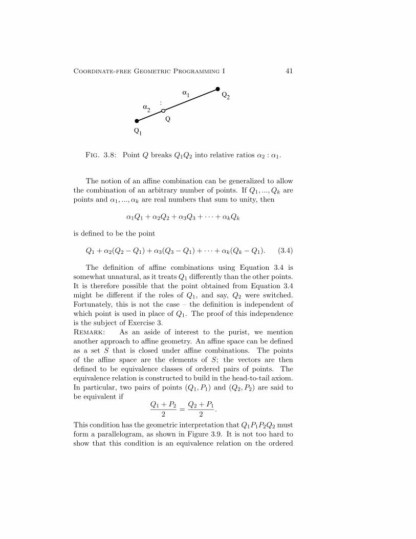
An expression such as Equation 3.3 is called an affine combina-tion. Affine combinations possess simple geometric interpretations.In particular, Equation 3.3 states that the point Q lies on the linesegment Q1, Q2 so as to break the segment into relative distancesα2 : α1, as shown in Figure 3.8. Conversely, if a point Q is knownto break a line segment Q1, Q2 into relative ratios a : b, then Q canbe expressed as
Q =bQ1 + aQ2
a + b,
where for the sake of generality we have not assumed that a and bsum to one.
Affine combinations are supported in the ADT by the routine:
• Point ← PPac( P, Q : Point; a, b : Scalar)The Point
a P + b Q.
is returned.
Q1
Q2
Q
α2:
α1
Coordinate-free Geometric Programming I 41
Fig. 3.8: Point Q breaks Q1Q2 into relative ratios α2 : α1.
The notion of an affine combination can be generalized to allowthe combination of an arbitrary number of points. If Q1, ..., Qk arepoints and α1, ..., αk are real numbers that sum to unity, then
α1Q1 + α2Q2 + α3Q3 + · · · + αkQk
is defined to be the point
Q1 + α2(Q2 −Q1) + α3(Q3 −Q1) + · · · + αk(Qk −Q1). (3.4)
The definition of affine combinations using Equation 3.4 issomewhat unnatural, as it treats Q1 differently than the other points.It is therefore possible that the point obtained from Equation 3.4might be different if the roles of Q1, and say, Q2 were switched.Fortunately, this is not the case – the definition is independent ofwhich point is used in place of Q1. The proof of this independenceis the subject of Exercise 3.Remark: As an aside of interest to the purist, we mentionanother approach to affine geometry. An affine space can be definedas a set S that is closed under affine combinations. The pointsof the affine space are the elements of S; the vectors are thendefined to be equivalence classes of ordered pairs of points. Theequivalence relation is constructed to build in the head-to-tail axiom.In particular, two pairs of points (Q1, P1) and (Q2, P2) are said tobe equivalent if
Q1 + P2
2=
Q2 + P1
2.
This condition has the geometric interpretation that Q1P1P2Q2 mustform a parallelogram, as shown in Figure 3.9. It is not too hard toshow that this condition is an equivalence relation on the ordered

Q1
Q2
P1
P2
42 Computer Graphics
Fig. 3.9: Points Q1P1P2Q2 forming a parallelogram.
pairs of points, implying that the set of all ordered pairs of points arepartitioned into equivalence classes. If [Q,P ] denotes the equivalenceclass containing the pair (Q,P ), then the set of all equivalence classesform a vector space, with scalar multiplication and addition definedas:
α[Q,P ] = [Q, (1 − α)Q + αP ], α ∈ � (3.5)
[Q1, P1] + [Q2, P2] = [Q1, P1 + P2 −Q2]. (3.6)
The elements of the vector space thus formed are the vectors of theaffine space. �
3.3. Euclidean Geometry
In affine geometry metric concepts such as absolute length, distance,and angles are not defined. This is demonstrated by the fact that upto this point we have not used these concepts in the development ofaffine geometry. However, in graphics and computer aided design, itis often necessary to represent metric information, for without thisinformation it is not possible to define right angles or to distinguishcircles from ellipses.
When metric information is added to an affine space, the resultis the familiar concept of a Euclidean space. In other words,a Euclidean space is a special case of an affine space in which

Coordinate-free Geometric Programming I 43
it is possible to measure absolute distances, lengths, and angles.Consequently, all results obtained for affine spaces also hold inEuclidean spaces. As simple examples, every triple of points in aEuclidean space obey the head-to-tail axiom, and the points of aEuclidean space are closed under affine combinations
3.3.1. The Inner Product In keeping with our algebraic ap-proach to geometry, we shall incorporate metric knowledge by in-troducing a new algebraic entity called an inner product. An innerproduct for an affine space A is a function that maps a pair of vectorsin A.V into the reals. Rather than using a notation such as f(�u,�v)to denote an inner product, we use the more familiar form 〈�u,�v〉.Such a bi-variate function must possess the following properties toachieve the status of an inner product:(i) Symmetry: For every pair of vectors �u,�v, 〈�u,�v〉 = 〈�v, �u〉.
(ii) Bi-linearity: For every α, β ∈ � and for every �u,�v, �w ∈ A.V,
• 〈α�u + β�v, �w〉 = α〈�u, �w〉 + β〈�v, �w〉.• 〈�u, α�v + β �w〉 = α〈�u,�v〉 + β〈�u, �w〉.
(iii) Positive Definiteness: For every �v ∈ A.V, 〈�v,�v〉 > 0 if �v is notthe zero vector, and 〈�0, �0〉 = 0.
A Euclidean space E can now be defined as an affine spacetogether with a distinguished inner product; that is, E = (A, 〈,〉).To comform more closely with standard practice, the inner productassociated with a particular Euclidean space will generally bedenoted by ·, and will generally be referred to as the dot product.Thus, we write u · v to stand for 〈u, v〉.
The dot product is used to define length, distance, and angles asfollows:
• The length of a vector:
|�v| :=√�v · �v.
• The distance between two points:
Dist(P,Q) := |P −Q| .
• The angle between two vectors:
Angle(�v, �w) := cos−1(
�v · �w|�v| |�w|
).

44 Computer Graphics
Associated with every non-zero vector �v is a unique vector vhaving unit length that points in the same direction as �v. The vectors�v and v are, of course, related by
v :=�v
|�v| .
The definition of angles allows us to define the notion ofperpendicularity or orthogonality. In particular, two vectors �v and�w are said to be perpendicular (or orthogonal) if �v · �w = 0. We canalso define the vectors to be parallel if v · w = 1, and anti-parallel ifv · w = −1.
In the important special case of Euclidean 3-spaces, it is con-venient to define another operation on vectors, namely the crossproduct. Given a pair of vectors �v and �w from a Euclidean 3-space,we define × by the equation
�v × �w = |�v| |�w| sin θn,
where θ is the angle between the vectors and n is the unique unitvector that is perpendicular to �v and �w such that �v, �w and n satisfythe “right hand rule.”
Since Euclidean spaces are so useful in practical applications,we have found it convenient to make the convention that the Spacedatatype actually represents a Euclidean space. That is, in the codefragment
Space Screen;World := SCreate( “World”, 3);
the variable World is a Euclidean space, meaning that it comes pre-equipped with an inner product. Thus, if v and w are Vectors inWorld, then VVDot(v,w) returns v·w. Also defined is a routineVVCross(v,w) that returns v×w.
3.4. Frames
To perform numerical computations and to facilitate the creationof geometric entities, we must understand how affine spaces arecoordinatized. In this section, we give two methods for imposingcoordinates on affine spaces: frames and simplexes. Each methodhas its advantages, but we have chosen to use frames in the ADT
Coordinate-free Geometric Programming I 45
since they are more familiar to those used to traditional approachesto geometric programming.
Let A = (P,V) be an affine n-space, let O be any point, and let�v1, · · · , �vn be any basis for A.V. We call the column tuple
(�v1, · · · , �vn,O)T =
⎛⎜⎜⎜⎜⎝
�v1...�vnO
⎞⎟⎟⎟⎟⎠
a frame for A. Frames play the same role in affine geometry thatbases play in vector spaces. The role of frames is more preciselyindicated by the next claim.
Claim 2. If F = (�v1, ..., �vn,O)T is a frame for some affine n-space, then every vector �u can be written uniquely as
�u = u1�v1 + u2�v2 + · · · + un�vn, (3.7)
and every point P can be written uniquely as
P = p1�v1 + p2�v2 + · · · + pn�vn + O. (3.8)
The sets of scalars (u1, u2, ..., un) and (p1, p2, ..., pn) are called theaffine coordinates of �u and P relative to F .
Proof: The unique representation of �u follows from the fact that(�v1, ..., �vn) forms a basis for A.V. From the definition of additionbetween points and vectors, there is a unique vector �w such that
P = �w + O.
Since (�v1, ..., �vn) is a basis for A.V, �w has a unique representation
�w = p1�v1 + p2�v2 + · · · + pn�vn.
Thus, P can be expressed uniquely as
P = p1�v1 + p2�v2 + · · · + pn�vn + O. �
The notions of unit vectors and orthogonality allow the identifi-cation of an important kind of frame for Euclidean spaces. A frame

46 Computer Graphics
(�e1, ...�en,O)T is said to be a Cartesian frame if the basis vectors areortho-normal; that is, if the basis vectors satisfy
�ei · �ej =
{1 if i = j;0 otherwise
Support for frames can be added to the ADT by introducing anew Frame data type, together with the routines:
• Frame ← FCreate( name : string; O : Point; v1,...,vk : Vector)Returned is a new frame whose origin is O and whose basisvectors are v1,...,vk. An error is signaled if (a) the points andvectors do not reside in a common space, or (b) if the vectorsdo not form a basis. The name field is intended to be used fordebugging purposes.
• Point ← PCreate( f : Frame; c1,...,ck : Scalar)Denoting the origin of f as f.org and the basis vectors asf.v1,...,f.vk, the Point
f.org + c1 * f.v1 + · · · + ck * f.vk
is returned.
• Vector ← VCreate( f : Frame; c1,...,ck : Scalar)The Vector
c1 * f.v1 + · · · + ck * f.vk
is returned.
• (c1,...,ck : Scalar) ← PCoords( p : Point; f : Frame)Return the coordinates of p relative to f. An error is signaledif p and f do not reside in a common Space.
• (c1,...,ck : Scalar) ← VCoords( v : Vector; f : Frame)Return the coordinates of v relative to f. An error is signaledif v and f do not reside in a common Space.
• Point ← FOrg( f : Frame)Return the origin of the frame f.
• Vector ← Fv( f : Frame; i : integer)Return the i-th basis vector of f (numbered starting at one).

Coordinate-free Geometric Programming I 47
There is still a sort of chicken and egg problem with the creationof Points and Vectors in the ADT. Points and Vectors can be createdif one has access to a Frame, but to create Frames one must haveaccess to a Point and a collection of Vectors forming a basis. Thisapparent circularity can be broken by making the convention thatwhen a Space is created with SCreate(), it comes pre-equipped witha Frame known as the “standard frame.” If S is a Space, its standardframe can be accessed as StdFrame(S).
Example 2. Consider the code fragment shown in Figure 3.10(a),the geometric interpretation of which is shown in Figure 3.10(b).Although the example is somewhat contrived, it does serve toillustrate a number of important points:
1. The Frame f2 is not Cartesian.
2. Although P and Q are created with respect to different Frames,the system is able to determine that f1 and f2 span the samespace, and hence P and Q reside in the same space. It thereforemakes geometric sense to construct the midpoint M of the linesegment PQ. The system is responsible for the bookkeepingrequired to construct a valid representation for M.
3. Since M is known to reside in S, its coordinates relative to anyFrame for S can be extracted. The first print statement willproduce (1.25, 1.0), and the second print statment will produce(−1.5, 1).
Equation 3.8 can be written in a more symmetric form as anaffine combination of n+1 points. Let Qi = O+�vi for i = 1, ..., n, setQ0 equal to O, and let p0 = 1−(p1+· · ·+pn). With these definitions,simple rearrangement allows Equation 3.8 to be rewritten as
P = p0Q0 + p1Q1 + · · · + pnQn, (3.9)
where, by construction, p0 + p1 + · · · + pn = 1. Since every pointcan be written uniquely in the form of Equation 3.8, every point canalso be written uniquely in the form of 3.9. In this form, the scalars(p0, ..., pn) are called the barycentric coordinates of P relative to then-simplex Q0, ..., Qn. An n-simplex is a collection of n+1 points suchthat none of the points can be expressed as an affine combination

f1
f2
P M Q
48 Computer Graphics
S : Space;f1, f2 : Frame;P, Q, M : Point;
S := SCreate( ”Screen”, 2);f1 := StdFrame(S);f2 := FCreate( PCreate(f1,1.5,0.5), VCreate(f1,0.5,0), VCreate(f1,0.5,0.5));
{ Create P relative to f1 }P := PCreate( f1, 0.5, 1.0);
{ Create Q relative to f2 }Q := PCreate( f2, 0, 1.0);
{ Compute the midpoint M }M := PPac( P, Q, 0.5, 0.5);
{ Extract coordinates of M relative to f1 and f2 }print( PCoords( M, f1)); print( PCoords( M, f2));
(a)
(b)Fig. 3.10: A code fragment and its geometric interpretation.
Coordinate-free Geometric Programming I 49
of the others. Thus, a 1-simplex is a line segment, a 2-simplex is atriangle, a 3-simplex is a tetrahedron, and so forth.
Vectors can also be represented in barycentric form as follows.By letting u0 = −(u1 + · · · + un), Equation 3.7 can be rewritten as
�u = u0Q0 + u1Q1 + · · · + unQn,
where, by construction, u0 + u1 + · · · + un = 0.Simplexes and barycentric coordinates therefore offer an alter-
nate method of introducing coordinates into an affine space. If thecoordinates sum to one, they represent a point; if the coordinatessum to zero, they represent a vector. The notion of barycentriccoordinates may at first seem somewhat obscure, but it is actuallyused in several situations in graphics and CAGD. We will find themuseful, for instance, when we consider projective transformations inSection 7.1. Simplexes and barycentric coordinates also have impor-tant uses in the theory of Bezier curves and surfaces (cf. [6, 9]).
3.5. *Matrix Representations of Points and Vectors
In the previous section it was shown that points and vectors canbe uniquely identified by their coordinates relative to a given frame.The most straightforward way to represent points and vectors in acomputer is then to simply store their coordinates as a 1 × n rowmatrix. However, for reasons that will only become fully apparentlater, it is more convenient to augment the row matrix with anadditional value that distinguishes between points and vectors [12].To allow this augmentation to proceed in a rigorous fashion, weextend the original set of axioms for an affine space A to include:
(iii) Coordinate Axiom: For every point P ∈ A.P, 0 · P = �0, thezero vector of A.V, and 1 · P = P .
Armed with this axiom, we can rewrite Equation 3.8 in matrixnotation as
P = p1�v1 + p2�v2 + · · · + pn�vn + 1 · O= (p1 p2 · · · pn 1)(�v1 �v2 · · · �vn O)T .
Notice that the last component in the row matrix essentially saysthat P is a point, which explains the mystery of the additional
50 Computer Graphics
coordinate that was encountered in Section 2.6. Vectors can berepresented in a similar fashion by rewriting Equation 3.7 as:
�u = u1�v1 + u2�v2 · · ·un�vn + 0 · O= (u1 u2 · · · un 0)(�v1 �v2 · · · �vn O)T .
Thus, vectors are represented as row matrices whose last componentis zero.1
Suppose that a point P has coordinates (p1, ..., pn, 1) relativeto a frame F = (�v1, ..., �vn,O)T . It is natural to ask: what are thecoordinates of P relative to a frame F ′ = (�v′1, ..., �v
′n,O′)T ? To answer
this question, we must find scalars p′1, ..., p′n such that
p′1�v′1 + · · · + p′n�v
′n + O′ = p1�v1 + · · · + pn�vn + O.
It is more convenient to write this equation in matrix notation as
(p′1 · · · p′n 1)
⎛⎜⎜⎜⎜⎝
�v′1...�v′nO′
⎞⎟⎟⎟⎟⎠ = (p1 · · · pn 1)
⎛⎜⎜⎜⎜⎝
�v1...�vnO
⎞⎟⎟⎟⎟⎠ . (3.10)
Each of the elements of F can be written in coordinates relative toF ′. In particular, let these coordinates be such that:
�vi = fi,1�v′1 + · · · + fi,n�v
′n
O = fn+1,1�v′1 + · · · + fn+1,n�v
′n + O′
for i = 1, ..., n. Substituting these equations into Equation 3.10 gives
( p′1 · · · p′n 1 )
⎛⎜⎜⎜⎜⎝
�v′1...�v′nO′
⎞⎟⎟⎟⎟⎠ =
1Those familiar with homogeneous coordinates are accustomed to adding an ad-ditional component when representing points. Note however that the addition of acomponent has been done here without having to mention homogeneous coordinates orprojective spaces. This is not simply a trick, for we are representing affine entities, notprojective ones. For instance, in the current context, a row matrix with a final compo-nent of zero represents a vector, whereas in projective geometry, a row matrix with afinal component of zero represents an ideal point (more commonly known as a point atinfinity).
Coordinate-free Geometric Programming I 51
( p1 · · · pn 1 )
⎛⎜⎜⎜⎜⎝
f1,1�v′1 + · · · + f1,n�v
′n
...fn,1�v
′1 + · · · + fn,n�v
′n
fn+1,1�v′1 + · · · + fn+1,n�v
′n + O′
⎞⎟⎟⎟⎟⎠ ,
which can be rewritten as
( p′1 · · · p′n 1 )
⎛⎜⎜⎜⎜⎝
�v′1...�v′nO′
⎞⎟⎟⎟⎟⎠ =
( p1 · · · pn 1 )
⎛⎜⎜⎜⎜⎝
f1,1 · · · f1,n 0...
. . ....
...fn,1 · · · fn,n 0fn+1,1 · · · fn+1,n 1
⎞⎟⎟⎟⎟⎠
⎛⎜⎜⎜⎜⎝
�v′1...�v′nO′
⎞⎟⎟⎟⎟⎠ .
Linear independence of the vectors �v′1, ..., �v′n can be used to deduce
that
( p′1 · · · p′n 1 ) = ( p1 · · · pn 1 )
⎛⎜⎜⎜⎜⎝
f1,1 · · · f1,n 0...
. . ....
...fn,1 · · · fn,n 0fn+1,1 · · · fn+1,n 1
⎞⎟⎟⎟⎟⎠ .
Thus, a change of coordinate systems can be accomplished via matrixmultiplication. Notice that the matrix used to affect the change ofcoordinates has rows consisting of the coordinates of the elements ofthe “old frame” (frame F) relative to the “new frame” (frame F ′).
3.6. Affine Transformations
The next geometric object to be added to our collection is the affinetransformation. Affine transformations are mappings between affinespaces that preserve the algebraic structure of the spaces. That is,affine transformations map points to points, vectors to vectors, andunder certain conditions, frames to frames.
To begin, let A and B be two affine spaces (it is sometimes thecase that A and B are the same space). A map F : A.P → B.Pis said to be an affine transformation (also called an affine map) ifit preserves affine combinations. That is, F is an affine map if the
52 Computer Graphics
condition
F (α1Q1 + · · · + αkQk) = α1F (Q1) + · · · + αkF (Qk) (3.11)
holds for all points Q1, ..., Qk and for all sets of α’s that sum to unity.(Notice the similarity between this definition and the definition oflinear transformation given in Appendix 1.) Examples of affine trans-formations include: reflections, shear transformations, translations,rotations, scalings, and orthogonal projections. Perspective projec-tions are not affine transformations, but they are projective transfor-mations (see Section 7.1).
Example 3. As a specific example of an affine transformation, con-sider the transformation T : A.P → A.P that performs translationalong a fixed vector �t. This transformation can be defined by
T (P ) = P + �t.
To show that T is an affine transformation, it suffices to show that
T (α1P1 + α2P2) = α1T (P1) + α2T (P2)
for every pair of points P1, P2, and for every α1, α2 such thatα1 + α2 = 1. This is not difficult to do, as the following derivationshows:
T (α1P1 +α2P2)
= (α1P1 + α2P2) + �t
= P1 + α2(P2 − P1) + �t def of affine comb
= (P1 + �t) + α2[(P2 − P1) + (�t− �t)]
= (P1 + �t) + α2[(P2 + �t) − (P1 + �t)] Claim 1(f)= T (P1) + α2(T (P2) − T (P1))= α1T (P1) + α2T (P2) def of affine comb
Induction on the number of terms in the affine combination can beused to show that T preserves arbitrary affine combinations.
An immediate consequence of their definition is that affinetransformations carry line segments to line segments, and hence,planes to planes and hyperplanes to hyperplanes. This can be seen
Coordinate-free Geometric Programming I 53
by noting that the line segment connecting the points Q1 and Q2
can be written in parametric form as the affine combination
Q(t) = (1 − t)Q1 + tQ2, t ∈ [0, 1]. (3.12)
The image of the segment under an affine map F is therefore
F (Q(t)) = (1 − t)F (Q1) + tF (Q2), t ∈ [0, 1], (3.13)
which is a parametric description of the line segment connectingthe images of Q1 and Q2. Equations 3.12 and 3.13 actually showsomething substantially stronger. In particular, they show that thepoint breaking the line segment Q1, Q2 into relative ratio t : (1−t) ismapped to the point that breaks F (Q1), F (Q2) into the same relativeratio, as shown in Figure 3.11. We therefore arrive at the importantfact that affine maps preserve relative ratios.
Another important fact about affine maps is that they arecompletely determined if the image of an n-simplex is known. Tosee this, let F : A.P → B.P be an affine map, let A be anaffine n-space, and let Q0, ..., Qn be an n-simplex in A. In theprevious section it was shown that every point in A can be writtenuniquely as P = p0Q0 + · · · + pnQn. The fact that F is affineimplies that F (P ) = p0F (Q0) + · · · + pnF (Qn), which is completelydetermined if the points F (Q0), ..., F (Qn), i.e., the image of thesimplex (Q0, ..., Qn), are known.
We can push the above argument further to yield anotherinteresting result. Suppose that S = (Q0, ..., Qn) is an arbitrarysimplex in A and that S′ = (Q′
0, ..., Q′n) is an arbitrary collection of
points in B, not necessarily forming a simplex. We claim that thereis a unique affine map from A to B that carries S into S′. The proofis immediate: existence follows by letting the map F in the previousparagraph be such that F (Qi) = Q′
i, for i = 0, ..., n; uniquenessfollows from the fact that every point has a unique barycentricrepresentation. In the case of affine planes (occurring when bothA and B are affine two-spaces), this result says that every pair oftriangles are related by a unique affine map. Similarly, every pair oftetrahedrons in an affine 3-space are related by a unique affine map.
In the introduction to this section it was claimed that affinetransformations carry points to points and vectors to vectors.However, affine transformations are currently defined only on points.

Q1
Q2
F(Q1)
Q
F(Q)
F(Q2)F
t
:
1-tt
:
1-t
54 Computer Graphics
Fig. 3.11: The action of an affine map on a line segment.
Fortunately, we can extend their domains to include the vectors aswell. Let F : A.P → B.P be an affine map, let �v be any vector inA.V, and let P and Q be any two points in A.P such that �v = P−Q.We define F (�v) to be the vector in B.V given by F (P ) − F (Q). Inequation form,
F (�v) ≡ F (P −Q) := F (P ) − F (Q).
Notice that the points P and Q used in the definition are not uniquein that there are many pairs of points whose difference is �v. To verifythat the definition of F (�v) is well-formed, it must be shown that ifP ,Q and P ′,Q′ are two pairs of points whose difference is �v, thenF (P ) − F (Q) = F (P ′) − F (Q′). We leave the proof as an excerise.
Since the domain of an affine map such as F : A.P → A.P canbe extended to include A.V, we consider F being defined on all ofA, and hence we write simply F : A → B.
Using the definition of the action of an affine map on vectors, itis also not difficult to show that F is a linear transformation on theset of vectors. That is, F satisfies
F (u1�v1 + · · · + un�vn) = u1F (�v1) + · · · + unF (�vn), (3.14)
for all u1, ..., un and for all �v1, ..., �vn. The proof of this fact is ratherinstructive in that it demonstrates a use of the head-to-tail axiom.We will show that F satisfies the following two conditions:
1. F (�v + �w) = F (�v) + F (�w).
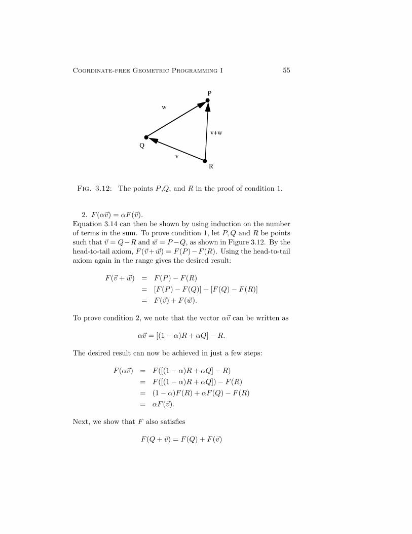
Q
w
P
R
v
v+w
Coordinate-free Geometric Programming I 55
Fig. 3.12: The points P ,Q, and R in the proof of condition 1.
2. F (α�v) = αF (�v).Equation 3.14 can then be shown by using induction on the numberof terms in the sum. To prove condition 1, let P,Q and R be pointssuch that �v = Q−R and �w = P−Q, as shown in Figure 3.12. By thehead-to-tail axiom, F (�v+ �w) = F (P )−F (R). Using the head-to-tailaxiom again in the range gives the desired result:
F (�v + �w) = F (P ) − F (R)
= [F (P ) − F (Q)] + [F (Q) − F (R)]
= F (�v) + F (�w).
To prove condition 2, we note that the vector α�v can be written as
α�v = [(1 − α)R + αQ] −R.
The desired result can now be achieved in just a few steps:
F (α�v) = F ([(1 − α)R + αQ] −R)
= F ([(1 − α)R + αQ]) − F (R)
= (1 − α)F (R) + αF (Q) − F (R)
= αF (�v).
Next, we show that F also satisfies
F (Q + �v) = F (Q) + F (�v)
56 Computer Graphics
for every point Q and every vector �v. To do this, let P be such that�v = P −Q. Thus, F (Q + �v) = F (Q + P −Q). Since the expressionQ + P −Q is an affine combination,
F (Q + P −Q) = F (Q) + F (P ) − F (Q)
= F (Q) + [F (P ) − F (Q)]
= F (Q) + F (�v).
Putting these facts together reveals that F preserves affine coordi-nates:
F (p1�v1 + · · ·+pn�vn +O) = p1F (�v1)+ · · ·+pnF (�vn)+F (O), (3.15)
showing that affine maps are completely determined once the imageof a frame is known.
Affine transformations can be manipulated in the geometric ADTby adding an AffineMap data type. The fact found above thatan affine map is completely determined once its action on a frameis known can be used as the basis of a coordinate-free method ofspecifying affine transformations. Specifically, we add to the ADTthe routines:
• AffineMap ← ACreate( f : Frame; O : Point, v1...vk :Vector)This is the most general affine map creation routine. Let Sdenote the space for which f is a frame, and let k denote S’sdimension. The point O and the vectors v1,...,vk must residein a common space S’; if they do not, an error is signaled.Returned is the (unique) affine map that carries f.org to O,f.v1 to v1, etc.
• Point ← PAxform( P : Point; T : AffineMap)If P resides in the domain space of T, then the image pointT(P) is returned; otherwise an error is signaled.
• Vector ← VAxform( v : Vector; T : AffineMap)If V resides in the domain space of T, then the image vectorT(v) is returned; otherwise an error is signaled.
Example 4.To demonstrate the use of the low-level affine map creation
routine ACreate() we use it to construct a higher-level routine that
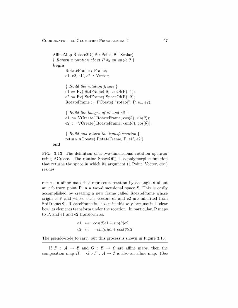
Coordinate-free Geometric Programming I 57
AffineMap Rotate2D( P : Point, θ : Scalar){ Return a rotation about P by an angle θ }begin
RotateFrame : Frame;e1, e2, e1’, e2’ : Vector;
{ Build the rotation frame }e1 := Fv( StdFrame( SpaceOf(P), 1);e2 := Fv( StdFrame( SpaceOf(P), 2);RotateFrame := FCreate( ”rotate”, P, e1, e2);
{ Build the images of e1 and e2 }e1’ := VCreate( RotateFrame, cos(θ), sin(θ));e2’ := VCreate( RotateFrame, -sin(θ), cos(θ));
{ Build and return the transformation }return ACreate( RotateFrame, P, e1’, e2’);
end
Fig. 3.13: The definition of a two-dimensional rotation operatorusing ACreate. The routine SpaceOf() is a polymorphic functionthat returns the space in which its argument (a Point, Vector, etc.)resides.
returns a affine map that represents rotation by an angle θ aboutan arbitrary point P in a two-dimensional space S. This is easilyaccomplished by creating a new frame called RotateFrame whoseorigin is P and whose basis vectors e1 and e2 are inherited fromStdFrame(S). RotateFrame is chosen in this way because it is clearhow its elements transform under the rotation. In particular, P mapsto P, and e1 and e2 transform as:
e1 �→ cos(θ)e1 + sin(θ)e2
e2 �→ − sin(θ)e1 + cos(θ)e2
The pseudo-code to carry out this process is shown in Figure 3.13.
If F : A → B and G : B → C are affine maps, then thecomposition map H = G ◦ F : A → C is also an affine map. (See
58 Computer Graphics
Exercise 7 on page 65.) We therefore add the following routine tothe ADT:
• AffineMap ← AACompose( F, G : AffineMap)Returned is the affine map G ◦ F. An error is signaled if thedomain of G does not match the range of F.
3.7. *Matrix Representations of Affine Transformations
Just as points and vectors can be represented as matrices, so toocan affine transformations. For notational simplicity, the followingdiscussion will be restricted to maps between affine planes. Thisrestriction is not limiting since all arguments carry through to affinespaces of arbitrary dimension.
Let A and B be two affine planes, let F : A �→ B be an affinetransformation, let (�v1, �v2,OA) be a frame for A, let (�w1, �w2,OB) bea frame for B, and let P be an arbitrary point whose coordinatesrelative to (�v1, �v2,OA) are (p1, p2, 1). We ask: what are thecoordinates of F (P ) relative to (�w1, �w2,OB)? The solution requireslittle more than simple manipulation. We begin by expanding P incoordinates and use the fact that F preserves affine coordinates:
F (P ) = F (p1�v1 + p2�v2 + OA) (3.16)
= p1F (�v1) + p2F (�v2) + F (OA). (3.17)
Since F carries vectors (points) in A into vectors (points) in B, thequantities F (�v1) and F (�v2) are vectors in B and the quantity F (OA)is a point in B, and as such they each have affine coordinates relativeto the frame (�w1, �w2,OB). Suppose that
F (�v1) = f1,1 �w1 + f1,2 �w2
F (�v2) = f2,1 �w1 + f2,2 �w2
F (OA) = f3,1 �w1 + f3,2 �w2 + OB
Using these coordinates, Equation 3.17 can be manipulated asfollows:
F (P ) = ( p1 p2 1 )
⎛⎜⎝ F (�v1)
F (�v2)F (OA)
⎞⎟⎠
Coordinate-free Geometric Programming I 59
= ( p1 p2 1 )
⎛⎜⎝ f1,1 �w1 + f1,2 �w2
f2,1 �w1 + f2,2 �w2
f3,1 �w1 + f3,2 �w2 + OB
⎞⎟⎠
= ( p1 p2 1 )
⎛⎜⎝ f1,1 f1,2 0
f2,1 f2,2 0f3,1 f3,2 1
⎞⎟⎠
⎛⎜⎝ �w1
�w2
OB
⎞⎟⎠
= ( p1 p2 1 )F
⎛⎜⎝ �w1
�w2
OB
⎞⎟⎠
= ( p′1 p′2 1 )
⎛⎜⎝ �w1
�w2
OB
⎞⎟⎠
Thus, the point P with coordinates (p1, p2, 1) gets transformed tothe point F (P ) with coordinates (p′1 p′2 1), where ( p′1 p′2 1 ) =( p1 p2 1 )F. For this reason, the matrix F is called the matrix rep-resentation of F relative to the frames (�v1, �v2,OA) and (�w1, �w2,OB).Notice that
• The first row of F is the representation of F (�v1).
• The second row of F is the representation of F (�v2).
• The third row of F is the representation of F (OA).As a consequence, affine maps are represented as matrices whose lastcolumn is (0 0 1)T . Conversely, every matrix whose last column is(0 0 1)T represents some affine transformation.
Example 5. As a specific example of the construction of a matrixrepresentation of an affine transformation, consider the constructionof a matrix representation of the translation T of Example 3. To dothis, we must pick frames in both the domain and the range. SinceT maps A onto itself, the domain and range are the same space, sowe may as well pick a single frame (�v1, �v2,O) to serve double duty.Suppose that in this frame the vector �t has the coordinates (a, b, 0).All we have to do to determine the matrix T is to determine whatT does to �v1, �v2, and O.
We’ll do the easy part first. The third row of T consists of thecoordinates of T (O), which are (a, b, 1) since
T (O) = O + �t

60 Computer Graphics
= a�v1 + b�v2 + O.
The first row of T consists of the coordinates of T (�v1). To seewhat these are, let R and S be two points such that �v1 = R − S.Then, by definition of how affine maps behave on vectors,
T (�v1) = T (R− S) by def of R,S= T (R) − T (S) by def T on vectors
= (R + �t) − (S + �t) by def of T= R− S by Claim 1(f)= �v1 by def of R,S.
In other words, T does not affect �v1. In fact, the derivation aboveworks for all vectors, not just �v1, so T does not affect any vector.This means that the first row of T is (1 0 0), and the second row is(0 1 0). Putting this all together, relative to the frame (�v1, �v2,O), Tis represented by the matrix
T =
⎛⎜⎝ 1 0 0
0 1 0a b 1
⎞⎟⎠ .
3.8. Ambiguity Revisited
In Section 3.1 it was claimed that the ADT solves the ambiguityproblem in that a given code fragment can have one and onlyone geometric interpretation. As a demonstration of how this isaccomplished, we refer again to the code fragment of Figure 3.1, thegeometric interpretations of which are shown in Figure 3.2.
Using the geometric ADT, each geometric interpretation isunambiguously reflected in the code. For instance, if the programmerintended a change of coordinates as indicated by Figure 3.2(a), theappropriate code fragment would be something like:
frame1, frame2 : Frame;P : Point;px, py : Scalar;
P := PCreate( frame1, p1, p2);(px,py) := PCoords( P, frame2);
Coordinate-free Geometric Programming I 61
where frame1 and frame2 are two frames having the geometricrelationship indicated in Figure 3.2(a). If the programmer wasinstead intending to effect a transformation on the space as indicatedby Figure 3.2(b), the appropriate code would be something like:
T : AffineMap;S : Space;P’, P : Point;sf : Frame;
...sf := StdFrame(S);T := ACreate( sf, FOrg(sf), SVMult(2,Fv(sf,1)), Fv(sf,2));
...P’ := PAxform( P, T);
...
Finally, if a transformation between separate spaces is to beapplied as indicated by Figure 3.2(c), the code would be somethinglike:
T : AffineMap;S1, S2 : Space;P’, P, O’ : Point;x’, y’ : Vector;
...{ Compute O’, x’, and y’ in S2 }
...T := ACreate( StdFrame(S1), O’, x’, y’);
...{ Not that P and P’ live in different spaces. }P’ := PAxform( P,T);
...
To reiterate, each of the code fragments above has an unam-biguous geometric interpretation that is undeniably apparent from
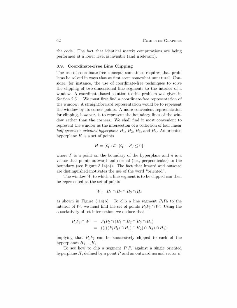
62 Computer Graphics
the code. The fact that identical matrix computations are beingperformed at a lower level is invisible (and irrelevant).
3.9. Coordinate-Free Line Clipping
The use of coordinate-free concepts sometimes requires that prob-lems be solved in ways that at first seem somewhat unnatural. Con-sider, for instance, the use of coordinate-free techniques to solvethe clipping of two-dimensional line segments to the interior of awindow. A coordinate-based solution to this problem was given inSection 2.5.1. We must first find a coordinate-free representation ofthe window. A straightforward representation would be to representthe window by its corner points. A more convenient representationfor clipping, however, is to represent the boundary lines of the win-dow rather than the corners. We shall find it most convenient torepresent the window as the intersection of a collection of four linearhalf-spaces or oriented hyperplane H1, H2, H3, and H4. An orientedhyperplane H is a set of points
H = {Q : �n · (Q− P ) ≤ 0}
where P is a point on the boundary of the hyperplane and �n is avector that points outward and normal (i.e., perpendicular) to theboundary (see Figure 3.14(a)). The fact that inward and outwardare distinguished motivates the use of the word “oriented”.
The window W to which a line segment is to be clipped can thenbe represented as the set of points
W = H1 ∩H2 ∩H3 ∩H4
as shown in Figure 3.14(b). To clip a line segment P1P2 to theinterior of W , we must find the set of points P1P2 ∩W . Using theassociativity of set intersection, we deduce that
P1P2 ∩W = P1P2 ∩ (H1 ∩H2 ∩H3 ∩H4)
= (((((P1P2) ∩H1) ∩H2) ∩H3) ∩H4)
implying that P1P2 can be successively clipped to each of thehyperplanes H1,...,H4.
To see how to clip a segment P1P2 against a single orientedhyperplane H, defined by a point P and an outward normal vector �n,

P
Q
(a)
H 1
W
(b)
n
Coordinate-free Geometric Programming I 63
Fig. 3.14: (a) The representation of a half-space as a point P andan outward pointing normal vector �n; (b) The representation of thewindow as the intersection of half-spaces.
it is convenient to think of the hyperplane as a function H : Points →� defined as
H(Q) = �n · (Q− P ). (3.18)
The convenient thing about this definition is that the value H(Q) isproportional to the signed distance of the point Q from the half-spaceboundary, with the constant of proportionality being the length of �n.That is, if dQ is the signed distance of Q to the half-space boundary,then H(Q) = |�n|dQ.
There are four cases of interest, depending on the signs ofH(P1) and H(P2). If both are positive, then both endpoints areoutside the half-space, meaning that the line segment can be triviallyrejected. If both are negative, then both endpoints are inside thehalf-space, meaning that the line segment can be trivially accepted.The interesting cases occur when the signs of H(P1) and H(P2)differ, implying that one endpoint is inside and the other is outside.Suppose that H(P1) > 0 and that H(P2) < 0 (the other case issymmetric and will not be discussed). We must therefore computethe intersection point I between the line segment and half-spaceboundary (see Figure 3.15). The intersection I can be computedeasily using an affine combination. Using similar triangles we findthat P1I : IP2 = H(P1) : −H(P2), meaning that
I =H(P1)P2 −H(P2)P1
H(P1) −H(P2).
P1
P2
IH(P1)
-H(P2)
H
64 Computer Graphics
Fig. 3.15: If one endpoint is inside the half-space, and one is outside,the point of intersection I must be computed.
Once I is computed, the subsegment P1I is discarded, and thesubsegment P2I is output as the result.
The above algorithm is the coordinate-free version of theSutherland-Hodgman line clipping algorithm [17].
Exercises
1. Show that the definition of the action of F on vectors is well-defined in the sense that if P,Q and P ′, Q′ are two pairs ofpoints such that P − Q = P ′ − Q′, then F (P ) − F (Q) =F (P ′) − F (Q′).
2. Let L1 and L2 be two lines that pass through the points Q1, P1
and Q2, P2 respectively. These lines are said to be parallel ifP1−Q1 is a scalar multiple of P2−Q2. Show that parallel linesare mapped to parallel lines under affine maps. (A degeneratecase can occur when both L1 and L2 are mapped to singlepoints.)
3. Show that the definition of affine combinations as given inEquation 3.4 is independent of which point is used in placeof Q1.
4. Show that scalar multiplication and addition of equivalenceclasses of points as in Equations 3.5 and 3.6 forms a vectorspace, then show that the axioms of affine spaces are satisfied.

0M
P
x
Coordinate-free Geometric Programming I 65
Fig. 3.16: The points P of an affine space as a translated vectorsubspace M
5. Let L be an �-dimensional vector space, let M be an m < n-dimensional vector subspace of L, let �x �∈ M be a vector in L,and let
P = {�x + �v : �v ∈ M}.
Figure 3.16 depicts the situation for n = 3 and m = 2. Definesubtraction on elements of P and a set V such that (P,V)form an affine space. Prove that the axioms of affine spacesare satisfied by your definition.
This exercise shows that affine spaces can be constructed bytranslating a vector subspace (M) away from the origin.
6. Write a pseudo-code statement of a procedure ARotate3D()that takes as input a point P, a vector v (both assumed toreside in an affine three space), and an angle θ. The procuedureshould return an AffineMap that represents rotation by θ aboutan axis through P in the direction of v. By convention, positiveangles correspond to clockwise rotation when viewed along v.
7. Show that if F : A → B and G : B → C are affine maps, thenthe composed map H = G ◦ F : A → C is also an affine map.
8. Let F : A → B be the unique affine map that carries theframe FA in A into the frame FB in B. Show that thematrix representation of F relative to FA and FB is the
66 Computer Graphics
identity matrix. (This implies that the identity matrix doesnot necessarily represent the identity transformation.)
9. Let F : A → B and G : B → C be affine maps, and let FA,FB,and FC be frames in A, B, and C, respectively. Show that if Fis the matrix representation of F relative to FA and FB, and Gis the matrix representation of G relative to FB and FC , thenFG is the matrix representation of G ◦ F .
10. Suppose that an affine map T : A → B has a matrixrepresentation T relative to frames FA and FB, and supposethat F ′
A is a frame in A such that coordinates relative to FAare changed into coordinates relative to F ′
A by multiplying bya matrix F. Show that the matrix representation of T relativeto F ′
A and FB is F−1 T .
11. Show that the function H(Q) defined in Equation 3.18 is anaffine map from points into real numbers. An affine map thatmaps into the reals is called an affine functional
12. (Due to Ron Goldman.) Show that every non-singular affinetransformation of the affine plane is the composite of onescale, one translation, one rotation, and one shear. A scaletransformation is one where O → O, �v1 → a�v1, and �v2 → b�v2,where (�v1, �v2,O) is a frame, and where a and b are non-zeroscalars. A shear is a transformation such that O → O, �v1 → �v1,�v2 → a�v1 + b�v2.
Linear Algebra 67
3.10. A Brief Review of Linear Algebra
A vector space over the reals is a set V, each element of which iscalled a vector, that satisfies the following properties:(i) Addition of vectors and multiplication by real numbers (scalars)
is defined.
(ii) The set is closed under linear combinations. That is, if �v, �w ∈ V ,and α, β ∈ �, then α�v + β �w ∈ V.
(iii) There is a unique zero vector �0 ∈ V, such that
• For every vector �v ∈ V, �0 + �v = �v.
• For every vector �v ∈ V, 0 · �v = �0.Some examples of vector spaces are listed below. For each
example, think about how multiplication and addition of vectorsis defined.
1. �2 = {(x, y)|x, y ∈ �}.
2. P 3 = the set of all polynomials of degree ≤ 3.
3. C([0, 1]) = the set of all continuous functions defined on theunit interval.
The vectors �v1, ..., �vk are said to be linearly independent if
c1�v1 + c2�v2 + · · · + ck�vk = �0 ⇔ ci = 0, i = 1, ..., k
where c1, ..., ck are scalars. Otherwise, the vectors are said to belinearly dependent.
The dimension of a vector space is defined to be the largestnumber of linearly independent vectors. For example, the dimensionof �2, written dim �2 can be shown to be 2, and dim P 3 can beshown to be 4.
A sequence (�v1, ..., �vn) of linearly independent vectors in a vectorspace of dimension n is called a basis. As a simple example, a basis for�2 is ((1, 0), (0, 1)). Another basis for �2 is ((1, 1), (0, 1)), and a basisfor P 3 is the familiar power basis (1, x, x2, x3). Another familiar basisfor P 3 are the cubic Bernstein polynomials (x3, 3x2(1 − x), 3x(1 −x)2, (1 − x)3).
Bases are essential for imposing coordinates on vector spaces.Their importance is underscored by the following theorem.
68 Computer Graphics
Theorem 3.10.1. Let (�v1, ..., �vn) be a basis for a vector spaceV. For every �w ∈ V , there exists a unique set of scalars c1, ..., cnsuch that
�w = c1�v1 + c2�v2 + · · · + cn�vn. (3.19)
The numbers (c1, ..., cn) are called coordinates of �w relative to thebasis (�v1, ..., �vn).
Proof. For a rigorous proof, see any standard text in linearalgebra such as O’Nan [14].
The two important points about this theorem are: (1) coordi-nates are always relative to some basis, and (2) relative to a partic-ular basis, the coordinates are unique. It is therefore meaninglessto talk about the coordinates of a vector without talking about thebasis relative to which the coordinates are taken.
Let V,W be vector spaces (in many graphics and CAGD appli-cations V and W are the same space). A map T : V �→ W is a lineartransformation if for every α1, ..., αk ∈ �, and for every �v1, ..., �vk ∈ V,
T (α1�v1 + α2�v2 + · · ·αk�vk) = α1T (�v1) + α2T (�v2) + · · · + αkT (�vk).
Exercises
1. For the vector space �2, what are the coordinates of (4, 3)relative to the basis ((1, 1), (0, 1))?
2. For the vector space P 3, what are the coordinates of 2x relativeto the basis (1, x, x2, x3)? What are the coordinates of 2xrelative to the basis (x3, 3x2(1 − x), 3x(1 − x)2, (1 − x)3)?
3. Show that a linear transformation T : V �→ W carries the zerovector in V into the zero vector in W.
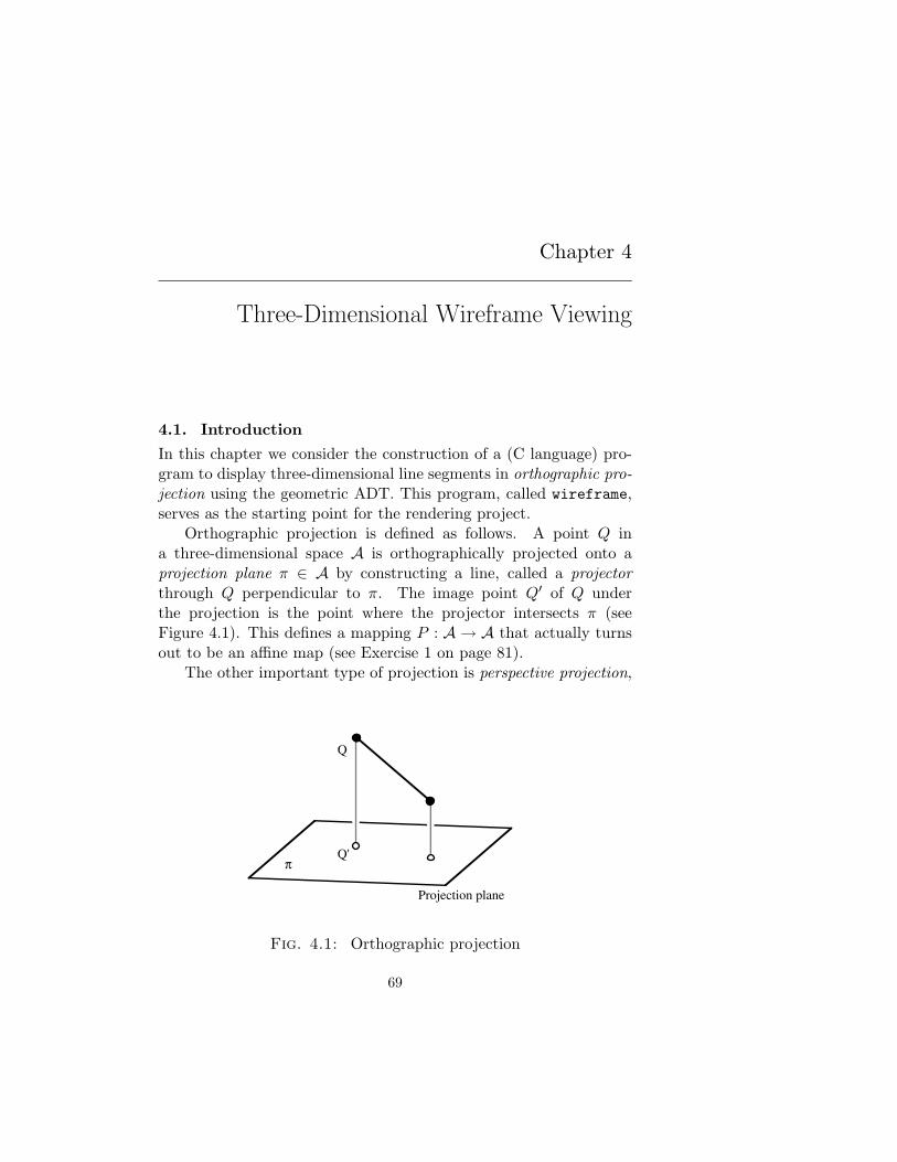
Q
Q'π
Projection plane
Chapter 4
Three-Dimensional Wireframe Viewing
4.1. Introduction
In this chapter we consider the construction of a (C language) pro-gram to display three-dimensional line segments in orthographic pro-jection using the geometric ADT. This program, called wireframe,serves as the starting point for the rendering project.
Orthographic projection is defined as follows. A point Q ina three-dimensional space A is orthographically projected onto aprojection plane π ∈ A by constructing a line, called a projectorthrough Q perpendicular to π. The image point Q′ of Q underthe projection is the point where the projector intersects π (seeFigure 4.1). This defines a mapping P : A → A that actually turnsout to be an affine map (see Exercise 1 on page 81).
The other important type of projection is perspective projection,
Fig. 4.1: Orthographic projection
69
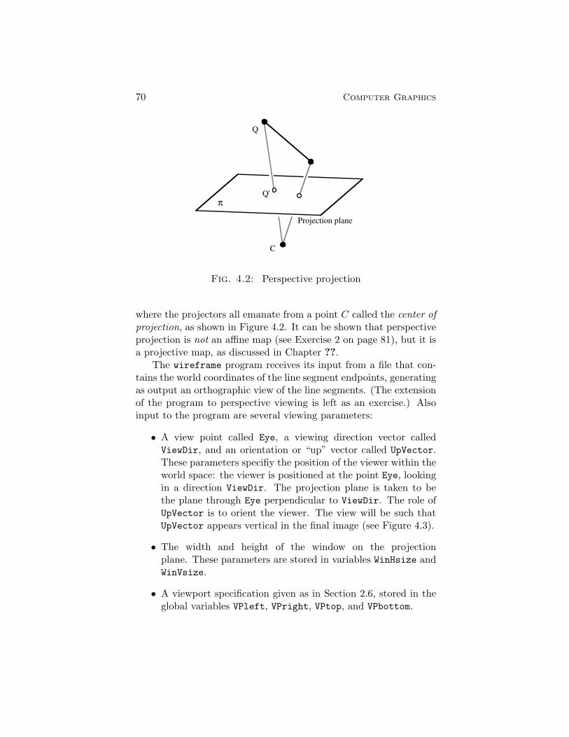
Q
Q'π
Projection plane
C
70 Computer Graphics
Fig. 4.2: Perspective projection
where the projectors all emanate from a point C called the center ofprojection, as shown in Figure 4.2. It can be shown that perspectiveprojection is not an affine map (see Exercise 2 on page 81), but it isa projective map, as discussed in Chapter ??.
The wireframe program receives its input from a file that con-tains the world coordinates of the line segment endpoints, generatingas output an orthographic view of the line segments. (The extensionof the program to perspective viewing is left as an exercise.) Alsoinput to the program are several viewing parameters:
• A view point called Eye, a viewing direction vector calledViewDir, and an orientation or “up” vector called UpVector.These parameters specifiy the position of the viewer within theworld space: the viewer is positioned at the point Eye, lookingin a direction ViewDir. The projection plane is taken to bethe plane through Eye perpendicular to ViewDir. The role ofUpVector is to orient the viewer. The view will be such thatUpVector appears vertical in the final image (see Figure 4.3).
• The width and height of the window on the projectionplane. These parameters are stored in variables WinHsize andWinVsize.
• A viewport specification given as in Section 2.6, stored in theglobal variables VPleft, VPright, VPtop, and VPbottom.

Eye
UpVector
ViewDir
StdFrame(Screen)
Viewport
World Screen
ViewTransformWindow
Three-Dimensional Wireframe Viewing 71
Fig. 4.3: Window and viewport specification.
The general strategy is to create two spaces, World and Screen.The World space is a Euclidean three-space in which the objectsto be viewed are placed. The Screen space is a two-dimensionalspace that corresponds to the physical frame buffer, with the visibleportion of the Screen space defined to be the unit square subtendedby the standard frame in Screen space (see Figure 4.3). A viewingframe (called ViewFrame) is constructed from the viewing parametersand a clipping volume is constructed about the viewing frame. Theclipping volume is a rectangular parallelpiped as shown in Figure 4.4.
Line segments are then processed in four steps:
1. Point Creation: When a pair of endpoint coordinates are readfrom the data file, they are immediately converted to Points inthe World space.
2. Clipping: The line segment between the newly created end-points is clipped to the clipping volume.
3. Transformation to Screen Space: The clipped line is (affinely)mapped into the Screen space.
4. Scan Conversion: The device coordinates of the clipped,projected line segment are extracted and scan converted usinga line drawing algorithm such as Bresenham’s algorithm.
We shall now examine each of these steps in more detail todemonstrate their implementation using the geometric ADT.
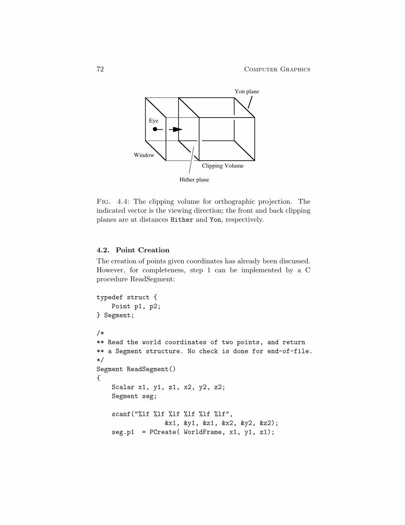
Window
Clipping Volume
Eye
Hither plane
Yon plane
72 Computer Graphics
Fig. 4.4: The clipping volume for orthographic projection. Theindicated vector is the viewing direction; the front and back clippingplanes are at distances Hither and Yon, respectively.
4.2. Point Creation
The creation of points given coordinates has already been discussed.However, for completeness, step 1 can be implemented by a Cprocedure ReadSegment:
typedef struct {
Point p1, p2;
} Segment;
/*
** Read the world coordinates of two points, and return
** a Segment structure. No check is done for end-of-file.
*/
Segment ReadSegment()
{
Scalar x1, y1, z1, x2, y2, z2;
Segment seg;
scanf("%lf %lf %lf %lf %lf %lf",
&x1, &y1, &z1, &x2, &y2, &z2);
seg.p1 = PCreate( WorldFrame, x1, y1, z1);
Three-Dimensional Wireframe Viewing 73
seg.p2 = PCreate( WorldFrame, x2, y2, z2);
return seg;
}
where WorldFrame is a synonym for StdFrame(World).
4.3. Clipping
In analolgy with Section 3.9, the clipping volume is represented as theintersection of a collection of (six) oriented hyperplanes as shown inFigure 4.4. Each hyperplane is represented as a point and an outwardpointing vector (or as described in Section 3.9 and Exercise 11 onpage 66, as affine functionals). In our implementation, hyperplanesare represented using the C structure
typedef struct {
Point b;
Normal n;
} Hyperplane;
For now it is sufficient to think about the datatype Normal as beinga Vector used specially to represent perpendicularity (we’ll comeback to this issue in the next chapter). Since we are thinking ofhyperplanes as affine functionals, we define a procedure to applythem to points:
/*
** Evaluate the affine functional associated with the
** Hyperplane Pi at the point q.
*/
Scalar EvalHyperplane(Pi, q)
Hyperplane Pi;
Point q;
{
return NVApply( Pi.n, PPDiff(q,Pi.b));
}
Don’t worry at this point about the meaning of NVApply; it issimply a pedantic way of writing VVDot.
The clipping volume is then defined to be the intersection ofthe negative half-spaces defined by the oriented hyperplanes. As inSection 3.9, line segments can be clipped to volumes defined in this

74 Computer Graphics
way by successively clipping them against each of the planes.The clipping of line segments to planes in three dimensions is
identical to the process described in Section 3.9. A C implementationof the algorithm to clip a line segment to a single hyperplane isshown below. Much of the code is devoted to correctly treatingthe boundary cases where one or both endpoints are sufficientlyclose to the boundary of the hyperplane that numerical error couldcause problems. The constant EPSILON is a predefined value that isintended to be an upper bound on numerical error.
/*
** Clip a line segment against the given Hyperplane.
** Return TRUE if a portion of the segment survives
** the clipping; return FALSE otherwise.
*/
static int ClipLineAgainstHyperplane( P, p1, p2)
Hyperplane P;
Point *p1, *p2;
{
Point lp1, lp2; /* Local copies of endpoints. */
Scalar pp1, pp2;/* H(p1) and H(p2) */
Point intersect;/* Point of intersection. */
lp1 = *p1;
lp2 = *p2;
pp1 = EvalHyperplane( P, lp1);
pp2 = EvalHyperplane( P, lp2);
/* If the endpoints are within EPSILON of */
/* the boundary treat them as if they are */
/* exactly on the boundary. */
if (fabs(pp1) < EPSILON) {
pp1 = 0.0;
}
if (fabs(pp2) < EPSILON) {
pp2 = 0.0;
}

Three-Dimensional Wireframe Viewing 75
/* At this point |pp1| and |pp2| are at */
/* least as big as EPSILON or exactly 0.0 */
/* so it is safe to test for equality */
/* with zero. */
if ((pp1 > 0.0) && (pp2 > 0.0)) {
/* Both points are outside --- trivial reject */
return FALSE;
}
if ((pp1 <= 0.0) && (pp2 <= 0.0)) {
/* Both points are inside --- trivial accept */
return TRUE;
}
/* Check to see if one of the endpoints is */
/* on the boundary. If so, then the line */
/* should either be trivially rejected or */
/* trivially accepted. */
if (pp1 == 0.0) {
if (pp2 > 0.0) {
/* lp1 is on the boundary, lp2 is */
/* outside: trivial reject */
return FALSE;
} else {
/* lp1 is on the boundary, lp2 is */
/* inside: trivial accept. This case */
/* should have been caught above, but*/
/* I’m paranoid. */
return TRUE;
}
}
if (pp2 == 0.0) {
if (pp1 > 0.0) {
/* lp2 is on the boundary, lp1 is */
/* outside: trivial reject */
return FALSE;
} else {
/* lp2 is on the boundary, lp1 is */
/* inside: trivial accept. This case */

76 Computer Graphics
/* should have been caught above, but */
/* I’m still paranoid. */
return TRUE;
}
}
/*-----------------------------------------------*/
/* The line segment definitely crosses the plane.*/
/* In fact, the Hyperplane cuts the line into */
/* ratios |pp1| to |pp2|. This is used */
/* to compute the point of intersection. */
/*-----------------------------------------------*/
intersect = PPrr( lp1, lp2, pp1, -1.0*pp2);
/* Figure out which endpoint to throw out */
if (pp1 < 0.0) {
/* Throw out lp2 */
*p1 = lp1;
*p2 = intersect;
} else {
/* Throw out lp1 */
*p1 = intersect;
*p2 = lp2;
}
return TRUE;
}
This routine points out that the coordinate-free implementationof clipping has the added benefit that the code has no notion ofthe dimension of the space in which the line segments live. Thismeans that the procedure above can be used for two-dimensional,three-dimensional, or even n-dimensional line clipping. In two-dimensional clipping, for instance, the oriented hyperplanes are theoriented lines that bound the visible window. Notice too that thehyperplanes are not required to be in any special orientation (as longas the clipping volume is convex). This allows irregular windows andclipping volumes to be used without increasing the complexity of thecode.
Three-Dimensional Wireframe Viewing 77
4.4. Transformation to Screen Space
The transformation that carries points in the World space intopoints in the Screen space should be such that the window onthe projection plane is carried into the viewport, as indicated byFigure 4.3. This transformation, called ViewTransform, is an affinemap since orthographic projection is assumed.
As described in Section 3.6, an affine transformation such asViewTranform is completely characterized once its action on a frameis known. The ViewFrame is set up for this purpose. The originof the ViewFrame is taken to be the point Eye, the x directionvector is taken to be the vector from Eye to the right edge ofthe window, the y direction vector is the vector from Eye to thetop of the window, and the z direction vector is the unit vector inthe direction of ViewDir. The convenience of this definition of theViewFrame is that we have a simple characterization for its imageunder ViewTransform. Specifically, let VPCenter denote the centerpoint of the viewport, and let VPx and VPy denote the vectors fromVPCenter to the right and top edges, respectively, of the viewport.The origin of ViewFrame (the Eye point) therefore maps to VPCenter,its x direction vector maps to VPx, its y direction vector maps toVPy, and its z direction vector maps to the zero vector in Screen.The global variable ViewTransform therefore be constructed fairlysimply:
BuildViewTransform()
{
Point VPCenter;
Vector VFx, VFy, VFz, VPx, VPy;
VFz = VNormalize( ViewDir);
VFx = SVMult(
VNormalize(VVCross(VFz,UpVector)),
WinHsize/2.0);
VFy = SVMult(
VNormalize(VVCross( VFx, VFz)),
WinVsize/2.0);
ViewFrame = FCreate("View",Eye,VFx,VFy,VFz);
VPCenter = PCreate( StdFrame(Screen),

78 Computer Graphics
(VPleft+VPright)/2.0,
(VPtop+VPbottom)/2.0);
VPx = VCreate( StdFrame(Screen),
(VPright-VPleft)/2.0, 0.0);
VPy = VCreate( StdFrame(Screen),
0.0, (VPtop-VPbottom)/2.0);
ViewTransform = ACreate( ViewFrame,
VPCenter, VPx, VPy,
VZero(Screen));
}
where VZero(S) returns the zero vector in the space S. Linesegments can then be mapped from the World space into the Screenspace by:
/*
** Send the segment "seg" through the viewing
** transformation.
*/
Segment TransformSegment( seg)
Segment seg;
{
Segment ScreenSegment;
ScreenSegment.p1 = PAxform( seg.p1, ViewTransform);
ScreenSegment.p2 = PAxform( seg.p2, ViewTransform);
return ScreenSegment;
}
4.5. Scan Conversion
Once the segment has been mapped to Screen space, scan conversioncan occur after the device coordinates for the endpoints havebeen determined. Using the geometric ADT, this is most easilyaccomplished by defining a “device frame” called DeviceFrame inthe Screen space. This frame is defined such that coordinatesrelative to the device frame represent device coordinates. As anexample, consider a device that has the origin in the upper left hand

Pixel grid
Od
sx
sy
dx
dy
Os
Three-Dimensional Wireframe Viewing 79
Fig. 4.5: The definition of the device frame (Od, �dx, �dy)T assuming
a device whose origin is in the upper left corner, with x increasingto the right and y downward. The vectors �dx and �dy are defined tobe the length and width of a pixel.
corner, with x coordinates increasing to the right and y increasingdownward. Suppose too that pixels are addressed from 0 to XRES inthe x direction and from 0 to YRES in the y direction.
Referring to Figure 4.3, the wireframe example establishes theconvention that the visible portion of the Screen space is theunit square subtended by StdFrame(Screen). Let the origin ofStdFrame(Screen) be denoted by Os, the x-direction vector by �sx,and the y-direction vector by �sy. If the device frame has origin Od,
x-direction vector �dx, and y-direction vector �dy, then (see Figure 4.5):
• Od = Os + �sy. This sets the origin of the device frame to theupper left hand corner of the visible region of Screen space.
• �dx = 1XRES
�sx. This says that device x-coordinates increase tothe right and range from 0 to XRES. In other words, the vector�dx is one pixel in length, as shown in Figure 4.5.
• �dy = − 1Ymax
�sy. This says that device y-coordinates increase todownward and range from 0 to YRES.
Having established DeviceFrame as an initialization step, a

80 Computer Graphics
segment in Screen space can be scan converted by extractingcoordinates relative to DeviceFrame, then invoking a standard scan-converter such as Bresenham’s algorithm:
DeviceInitialize()
{
Point Os,Od;
Vector Xs, Ys, dx, dy;
Os = FOrg(StdFrame(Screen));
Xs = Fv(StdFrame(Screen), 1);
Ys = Fv(StdFrame(Screen), 2);
Od = PVAdd( Os, Xs);
dx = SVMult( 1/XRES, Xs);
dy = SVMult( -1/YRES, Ys);
DeviceFrame = FCreate( "Device", Od, dx, dy);
}
/*
** Draw a segment on the device by extracting
** device coordinates then calling Bresenham’s
** algorithm.
*/
DeviceDrawLine(seg)
Segment seg;
{
Scalar x1, y1, x2, y2;
/* Extract coords relative to DeviceFrame */
PCoords( DeviceFrame, seg.p1, &x1, &y1);
PCoords( DeviceFrame, seg.p2, &x2, &y2);
/* ... and draw the line. */
Bresenham((int)x1,(int)y1,(int)x2,(int)y2,BLACK);
}

Three-Dimensional Wireframe Viewing 81
Exercises
1. Show that orthographic projection preserves affine combina-tions, and is therefore an affine map.
2. Show that perspective projection is not an affine map.

82 Computer Graphics

Chapter 5
Hierarchical Modeling
In this chapter we take a first look at methods for representingstructured (i.e., hierarchical) collections of geometric models thatcontain sufficient information to allow the creation of smooth shadedcolor images with hidden surfaces removed.
5.1. Simple Polygons
Line segments are insufficient as modeling primitives for creatingrealistic images since they do not contain enough information toremove hidden surfaces. A two-dimensional modeling primitive musttherefore be introduced. The simplest such primitive is a triangle.More generally, one could use quadrilaterals or polygons with anarbitrary number of vertices. More complex objects such cubes,chairs, telephones, etc., can be tiled using polygonal facets. Webegin with the definition of the notion of a “simple” polygon.
A curve is said to be simple if it does not intersect itself. TheJordan curve theorem says that a closed simple planar curve dividesthe plane into two sets, a finite “inside” and an infinite “outside”[7]. A simple polygon P can be defined as the finite set bounded bya closed, simple, planar, piecewise linear curve.
A simple polygon P is typically represented by a sequence ofco-planar vertices V1, ..., Vn. The bounding edges of the polygon aretherefore the line segments ViVi+1, i = 1, ..., n, where indices areto be taken modulo n. Simple polygons can be either convex orconcave. A convex polygon is one where the points of the polygonform a convex set (a set S is convex if its elements are closed underconvex combinations).
Since we are interested in using simple polygons as modeling
83

Window
Polygon
A
B
C
D
84 Computer Graphics
Fig. 5.1: There is more to polygon clipping than repeated lineclipping. Repeated line clipping would result in the vertices A, B,and C. However, the vertices of the clipped polygon are A, B, C andD. Thus, further processing would be required to determine that Dis the vertex that needs to be added to complete the description ofthe clipped polygon.
primitives, we must develop algorithms for processing them throughthe graphics viewing pipeline. That is, we must develop algorithmsfor clipping, transforming, and scan-converting simple polygons. Theremainder of this section is devoted to these tasks.
5.1.1. Clipping The problem we consider first may be stated as:
Given: A convex simple polygon P with verticesV1, ..., Vn contained in a two-dimensional space A, anda convex window W (the clipping region) represented asthe intersection of oriented hyperplanes H1, ..., Hk.
Find: The vertices V ′1 , ..., V
′n′ of the polygon P ′ = P∩W .
One might be tempted to solve this problem by using theSutherland-Hodgman line clipping algorithm to clip the edge V1V2
to W , then V2V3 to W , and so on, to produce a sequence ofvertices V ′
1 , ..., V′n′ that would be conjectured to form the vertices of
P ′ = P ∩W . The failure of this approach is indicated in Figure 5.1.The algorithm we present here is due to Sutherland and Hodg-
man [17]. It proceeds as in the Sutherland-Hodgman line clipping

I
I
p
Hp
s
Output(p)1) p ∈H, s ∈H
Case Geometry Action
H p None
Hp Output(I)
Output(p)
Output(I)
3) p ∈H, s ∉H
4) p ∉H, s ∈H
2) p ∉H, s ∉H
s
s
Hs
Hierarchical Modeling 85
Fig. 5.2: A summary of the Sutherland-Hodgman polygon clippingalgorithm.
algorithm in that it successively clips the entire polygon to each ofthe oriented hyperplanes defining the clipping region. The problemof clipping a polygon to a convex clipping region is thereby reducedto the following problem:
Given: A polygon P with vertices V1, ..., Vn to anoriented hyperplane H.
Find: The vertices of Q1, ..., Qm of P ∩H.
The method is to march around the vertices of P keeping track ofa previous vertex s and a current vertex p. One each iteration of thealgorithm, there are four cases to consider based on the containmentof s and p in H. The action to take in each of the cases is summarizedin Figure 5.2. The action Output(Q) adds point Q to the end of thesequence of vertices Q1, ..., Qm being built up for P ∩H.
86 Computer Graphics
This same algorithm extends readily for clipping polygons in anaffine space A of arbitrary dimension to a clipping region representedas the intersection of oriented hyperplanes.
The proper clipping of concave polygons is somewhat moredifficult. Such an algorithm has been developed by Weiler andAtherton [22].
5.1.2. Transforming Through Affine Maps The image of asimple polygon P with vertices V1, ..., Vn under an affine transforma-tion T is again a simple polygon P ′ with vertices T (V1), ..., T (Vn). Apolygon can therefore be mapped through an affine transformationsimply by mapping each of its vertices.
5.1.3. Scan-Conversion In this section we examine two algo-rithms for scan-converting polygons. The first is a general algorithmappropriate for scan-converting a simple polygon with an arbitrarynumber of edges. The second algorithm is a simplified version op-timized for scan-converting triangles. In the following sections weassume that the vertices are given in device coordinates.
A Sweep Line Algorithm The basic idea in this algorithm is toprocess the polygon a scan-line at a time, considering the scan-linesin, say, bottom to top order. For each scan-line, all intersectionsI0, ..., Ik−1 between the scan-line and the edges of the polygon arefound. The intersections are maintained in a list sorted by increasingx coordinate. For each pair of intersection points I2i, I2i+1, all pixelsbetween these points (called a span) are illuminated as indicated inFigure 5.3.
One subtlety with the algorithm is that intersections between thepolygon and the scan-line must be counted carefully since there isan implicit assumption that the number of intersections I0, ..., Ik−1
is even. Consider for instance scan-lines S2 and S3 in Figure 5.3.Vertex V3 is counted twice on scan-line S2 whereas the vertex V1
is counted only once in scan-line S3. The general rule is to counta vertex twice if it is a local min or a local max; it is counted onceotherwise. A vertex Vi is considered a local min if both Vi−1 and Vi+1
lie on scan-lines above Vi; local max vertices are defined similarly.1
The real cleverness in the algorithm comes from the way the
1You should think about how to handle horizontal edges.
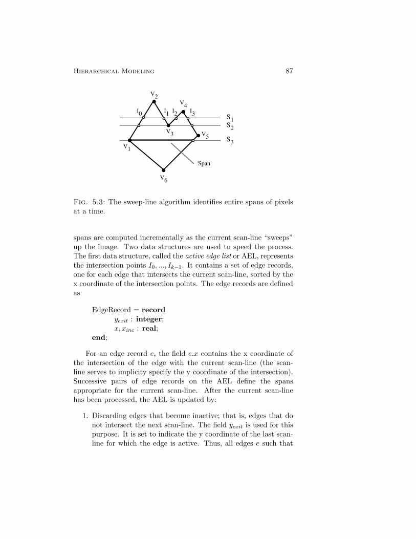
V5
V1
I1 I2 S1S2
S3
I0 I3
V6
V2
V3
V4
Span
Hierarchical Modeling 87
Fig. 5.3: The sweep-line algorithm identifies entire spans of pixelsat a time.
spans are computed incrementally as the current scan-line “sweeps”up the image. Two data structures are used to speed the process.The first data structure, called the active edge list or AEL, representsthe intersection points I0, ..., Ik−1. It contains a set of edge records,one for each edge that intersects the current scan-line, sorted by thex coordinate of the intersection points. The edge records are definedas
EdgeRecord = recordyexit : integer;x, xinc : real;
end;
For an edge record e, the field e.x contains the x coordinate ofthe intersection of the edge with the current scan-line (the scan-line serves to implicity specify the y coordinate of the intersection).Successive pairs of edge records on the AEL define the spansappropriate for the current scan-line. After the current scan-linehas been processed, the AEL is updated by:
1. Discarding edges that become inactive; that is, edges that donot intersect the next scan-line. The field yexit is used for thispurpose. It is set to indicate the y coordinate of the last scan-line for which the edge is active. Thus, all edges e such that

88 Computer Graphics
BuildBucketTable(P )begin
foreach edge (xi, yi)(xi+1, yi+1) ∈ P doe := new EdgeRecord;if (yi > yi+1) then
{ Make sure (xi, yi) is lowest endpoint. }Swap (xi, yi) and (xi+1, yi+1)
endif;e.x := x1;e.xinc := (xi+1 − xi)/(yi+1 − yi);Insert e into Byi in sorted order.
endforeach;end;
Fig. 5.4: Creation of the y-bucket table.
e.yexit is less than the y coordinate of the next scan-line areremoved from the AEL.
2. Updating the x coordinates of the intersections by adding xincto x. The values e.x and e.xinc for an edge e are initialized asshown in Figure 5.4.
3. Adding newly active edges. A second data structure, calledthe y-bucket table, is used to quickly identify the edges thatbecome active on a given scan-line. The y-bucket table is anopen hash table containing one bucket Bi per scan-line. It isinitialized by building an edge record per edge of the polygonas shown in Figure 5.4. An edge e is placed in bucket Bi if iis the y coordinate of the lowest endpoint of e. Edges withineach bucket are sorted by increasing x field as a primary sortkey and by increasing xinc value as a secondary sort key. Anexample of the y-bucket table is shown in Figure 5.5.
Scan-conversion of Triangles The scan-conversion of trianglesis much simpler than the scan-conversion of an arbitrary simplepolygon. Consider the scanning of a triangle with vertices V1 =(x1, y1), V2 = (x2, y2), V3 = (x3, y3). Without loss of generality we

e3e4
e3
0
1
2
3
4
5
6
7
e4
e5
e1
e2
e5
e2
e1
xi1
V1 = (x1,y1)
V3 = (x3,y3)
V2 = (x2,y2)
T1
T2
xi2
xi3
Hierarchical Modeling 89
Fig. 5.5: An example of the y-bucket table
Fig. 5.6: Triangle scan-conversion

90 Computer Graphics
can assume that y1 ≤ y2 ≤ y3. We divide the triangle along thescan-line through V2 into two subtriangles T1 and T2 as shown inFigure 5.6. The original triangle can be scanned by first scanningout T1 starting at V1 and moving upward, followed by scanning ofT2. The two intersections between the current scan-line and thetriangle are maintained and incrementally updated. This process issummarized by the following pseudo-code:
ScanTriangle(x1,y1,x2,y2,x3,y3 : integer){ Scan the triangle assuming y1 ≤ y2 ≤ y3 }begin
y, i : integer;inc1, inc2, inc3, xi1, xi2, xi3 : real;
if (y3 = y1) then{ The triangle is degenerate; scan the edges. }ScanSpan( min(x1,x2,x3), max(x1,x2,x3), y1);return;
endif;
xi2 := x1;inc2 := (x3 - x1)/(y3 - y1);
if (y1 �= y2) then{ Scan T1 }xi1 := x1;inc1 := (x2 - x1)/(y2 - y1);
{ Scan up to, but not including, scan-line y2. }{ Scan-line y2 will be scanned in the conversion }{ of subtriangle T2 }for y := y1 to y2-1 do
ScanSpan( xi1, xi2, y);xi1 := xi1 + inc1;xi2 := xi2 + inc2;
endfor;endif;
if (y2 �= y3) then
Hierarchical Modeling 91
{ Scan T2 }inc3 := (x3 - x2)/(y3 - y2);xi3 := x2;for y := y2 to y3 do
ScanSpan( xi2, xi3, y);xi2 := xi2 + inc2;xi3 := xi3 + inc3;
endfor;else
{ T2 was empty; scan out scan-line y2 }ScanSpan( xi1, xi2, y2);
endif;end;
The routine ScanSpan() referred to above is responsible forscanning the pixels on scan-line y. A strategy for avoiding gapsbetween triangles that are supposed to abut is to have ScanSpan()scan the pixels whose x coordinates are from the floor of the leftendpoint of the span to the ceiling of the right endpoint. This tendsto enlarge the triangle slightly , but it helps to fill gaps that canopen between triangles if both left and right endpoint coordinatesare rounded.
5.2. Object Hierarchies See transparencies5.2.1. Transformation Stacks
Exercises
1. Show that the Sutherland-Hodgman polygon clipping algo-rithm can fail if the polygon P to be clipped is concave.
2. Modify the triangle scan-conversion algorithm so that pixelscovered by abutting triangles are painted once and only once.

92 Computer Graphics

Chapter 6
Hidden Surface Algorithms
In this chapter we consider the problem of accounting for total orpartial occlusion of one object by another. That is, we consider thehidden surface problem. Hidden surface algorithms can be classifiedinto two broad categories: image space or object space algorithms.Image space algorithms resolve the hidden surface problem at theresolution of the final image; that is, only at displayable pixels.Object space algorithms, on the other hand, produce a resolutionindependent solution.
6.1. Back Face Culling
Before discussing general hidden surface algorithms that determinecomplete visibility information, there is a test that can often be usedto quickly identify invisible polygons. The test, known as back faceculling, is based on the assumptions that polygons are used to tileclosed opaque objects, and that none of the polygons of an objectare clipped by the clipping volume. In other words, the polygonspresent after clipping are assumed to enclose well-defined volumes.Back frace culling is therefore inappropriate for an object such asthe one shown in Figure 6.2 where polygons cover only five of thesix sides of a cube.
The test also requires that polygons have associated outward nor-mals that point outward from the enclosed volume (see Figure 6.1).It is common to infer the outward normal by imposing an orderingon polygon vertices. A common convention (for convex polygons) isthe “right hand rule”: if the polygon is defined by vertices V1, ..., Vn,then for any i = 1, ..., n the outward normal is defined to point along(Vi+1 − Vi) × (Vi+2 − Vi+1).
93

Eye ViewDir
Outwardnormals
94 Computer Graphics
Fig. 6.1: Back face culling.
Fig. 6.2: An object for which back face culling is inappropriatesince the polygons do not enclose a volume.

Hidden Surface Algorithms 95
With these conventions, the outward normal of a polygon canbe used to quickly determine a sufficient condition for invisibilityof the polygon. Intuitively, if the outward normal points awayfrom the viewer, then the polygon will be totally occluded by oneor more other polygons, and hence it can be culled from furtherprocessing. More specifically, a polygon can be culled in this way if(P −Eye) · �n > 0, where P is any point in the plane of the polygon,Eye is the viewpoint, and �n is the outward normal. This test is onlya sufficient condition for invisibility. The full necessary and sufficientconditions require a general purpose hidden surface algorithm.
6.2. Three-Dimensional Screen Space
Most hidden surface algorithms in use today are of the image spacevariety, resolving the hidden surface problem during scan-conversion.To use such an algorithm, we must extend the graphics pipelinesince the current pipeline projects from the three-dimensional worldspace down to the two-dimensional screen space, thus loosing criticalinformation about relative depth. If an image space algorithm is tobe used, the screen space must be generalized from two dimensions tothree dimensions, and the viewing transformation from world spaceto screen space must be set up so the depth ordering of objects (asseen from the viewpoint) is preserved.
To simplify the following discussion, we assume for the time beingthat the scene is to be viewed in orthographic rather than perspectiveprojection. The extension to perspective viewing will be covered inSection 7.2.
The geometric situation is indicated in Figure 6.3. By setting upthe viewing transformation so that it maps the clipping volume tothe indicated parallelpiped in the screen space (called the view box),when objects are transformed through the map their depth orderingsare preserved. Since the screen space is now three-dimensionalinstead of two-dimensional, the definition of the device frame mustbe extended to include a third vector. It is convenient to introducethe third device frame vector �dz as shown in Figure 6.3. In Figure 6.3,the standard frame for the screen space is (�sx, �sy, �sz,Os)
T , and the
device frame is denoted by (�dx, �dy, �dz,Od)T . Assuming the same type
of device as in Section 4.5, we have the relations
Od = Os + �sy

Clipping Volume
View box
World
ViewTransform
Screen
sx
sy
sz
dz
ViewFrame
96 Computer Graphics
Fig. 6.3: The viewing transformation is such that the clippingvolume is mapped to the view box so as to preserve the depthordering of points along projectors.
�dx =1
XRES�sx
�dy = − 1
YRES�sy
�dz = −�sz.
These frames have been set up so that if we transform a pointinto the screen space and extract coordinates (x, y, z) relative to thedevice frame, then (x, y) determines the pixel to illuminate, and zreflects the relative depth of the point within the scene such thatincreasing z corresponds to increasing depth. Thus, if two pointsP1 and P2 have device frame coordinates (x, y, z1) and (x, y, z2),respectively, then P1 occludes P2 if and only if z1 < z2.
6.3. The Depth Buffer Algorithm
The first hidden surface algorithm we shall consider is a very simpleone called the depth buffer algorithm. The algorithm, originated byEd Catmull in 1974 [4], is also called the z-buffer algorithm.
The basic idea behind the algorithm is to maintain an arrayof depth values during the scan-conversion of the primitives in thescene. The depth buffer allocates one entry for each pixel (x, y),denoted depth[x, y], that contains the depth (i.e., the “z-value”) of
Hidden Surface Algorithms 97
the nearest object covering pixel (x, y) that has been processed thusfar. The depth buffer is initialized by setting each entry to a valuelarger than any realizable depth. (The arrangement described inSection 6.2 guarantees that the largest possible depth is 1.) Duringthe scan-conversion of a primitive object O, if O is determined tocover pixel (x, y), then O is visible at (x, y) if and only if the depth ofO at (x, y) is less than the current value of depth[x, y]. If O is visibleat (x, y), then the pixel is shaded and the depth buffer is updatedto record the fact that O is now the closest object visible at (x, y).This process is summarized by the code fragment:
if depth of O at (x, y) < depth[x, y] thenfb writePixel(x, y, Shade( O, x, y));depth[x, y] := depth of O at (x, y);
endif
The Shade() routine implements one of the shading algorithmsdescribed in Chapter 8.
The depth buffer algorithm is very easy to implement, especiallyif the scene is tessellated into triangles prior to scan-conversion. Tothis end, the triangle scan-conversion algorithm of Section 5.1.3 canbe extended to incrementally compute the depth of the triangleduring scan-conversion (see Exercises 4 and 5 on page 100). Infact, the depth buffered scan-conversion of triangles is simple enoughthat a number of graphics workstations currently implement itin hardware. Another advantage of the depth buffer algorithmis that it is an on line algorithm, meaning that it can fullyprocess display primitives one at a time. Most other hiddensurface algorithms require that all primitives be available before anyocclusion determinations can be made.
A major disadvantage of the depth buffer algorithm, at least asdescribed above, is that the images it creates suffer from discretiza-tion effects. For instance, if two triangle interpenetrate, the line ofintersection will appear as a fairly ragged edge.
6.4. Warnock’s Algorithm
Warnock’s algorithm [20] is an early example of a divide and conquermethod that resolves hidden surfaces for the entire viewport bydetermining if the image to be rendered is “sufficiently simple” to
98 Computer Graphics
allow hidden surfaces to be determined with simple tests. If theimage within the viewport is too complex, the viewport is splithorizontally and vertically into four subviewports, the polygons aresplit and distributed amongst the subviewports, and the algorithmis called recursively.
Recursion stops when either a subviewport is the size of a pixelor the image within the subviewport is “simple”. An image withina subviewport is considered to be simple if at most one polygonis visible within the subviewport. This can occur either if thesubviewport contains at most one polygon or if the subviewport iscovered by a single polygon. If the subviewport is the size of a pixeland the image is not simple, the pixel is painted based on the colorof the nearest polygon covering the center of the pixel.
6.5. A Sweep Line Algorithm
In the late 60’s and early 70’s a number of algorithms were developedthat build up an image a scan-line at a time [1, 2, 21, 24]. The basicidea behind these algorithms is to use the sweep line algorithm forpolygon scan-conversion discussed in Section 5.1.3. In the followingit is assumed that the polygons do not interpenetrate. (If polygonsP1 and P2 do interpenetrate, P1 can be split along the plane ofP2 into two subpolygons using the Sutherland-Hodgman polygonclipping algorithm.)
The y-bucket table and active edges lists will again be used asin Section 5.1.3, with the exception that all edges of all polygonsare dealt with simultaneously. Thus, the y-bucket table is initializedby inserting an edge record for each edge in the scene. The edgerecords are essentially as before, with an added field that pointsback to a polygon record indicating which polygon the edge belongsto. Polygon records store data such as the plane equation for thepolygon, color attributes, and so forth.
The active edge list (AEL) is again used to maintain the setof edges intersected by the current scan-line, sorted in left to rightorder. The critical observation in the algorithm is that visibilitychanges can occur only at points of intersection between the scan-lineand elements of the AEL (this is only true because of the assumptionof non-interpenetrating polygons). This observation means that thehidden surface problem can be resolved for entire spans at a time.Referring to Figure 6.4, span s1 will be painted the color of polygon
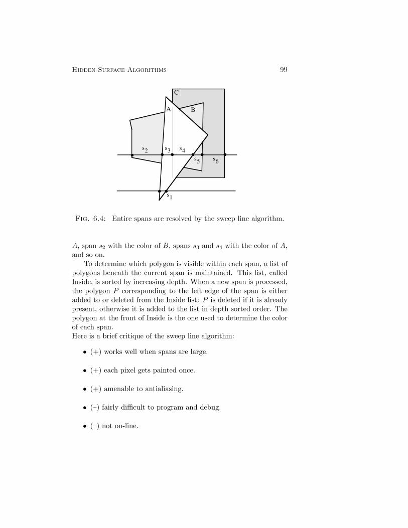
B
C
A
s2
s1
s3 s4s5 s6
Hidden Surface Algorithms 99
Fig. 6.4: Entire spans are resolved by the sweep line algorithm.
A, span s2 with the color of B, spans s3 and s4 with the color of A,and so on.
To determine which polygon is visible within each span, a list ofpolygons beneath the current span is maintained. This list, calledInside, is sorted by increasing depth. When a new span is processed,the polygon P corresponding to the left edge of the span is eitheradded to or deleted from the Inside list: P is deleted if it is alreadypresent, otherwise it is added to the list in depth sorted order. Thepolygon at the front of Inside is the one used to determine the colorof each span.Here is a brief critique of the sweep line algorithm:
• (+) works well when spans are large.
• (+) each pixel gets painted once.
• (+) amenable to antialiasing.
• (–) fairly difficult to program and debug.
• (–) not on-line.
100 Computer Graphics
Exercises
1. Show that if after clipping polygons tile closed opaque objects,then a polygon is occluded if (P − Eye) · �n > 0, where P is apoint on the polygon, �n is the outward pointing normal, andEye is the view point.
2. The right hand rule given in Section 6.1 is appropriate forconvex polygons only. Give a more general rule that can beapplied to concave as well as convex polygons.
3. For what class of scenes is back face culling both necessary andsufficient for polygon invisibility?
4. In the depth buffered scan conversion of triangles a “z incre-ment” must be computed such that if the triangle has depth zat pixel (x, y), then it has depth z + zinc at pixel (x + 1, y).(x, y and z denote three-dimensional device coordinates.) Ifthe triangle has vertices V1, V2, and V3 in screen space, showthat
zinc = −�dx · �n�dz · �n
where �dx and �dz denote device frame basis vectors as inFigure 6.3, and where �n is a vector perpendicular to the planeof the triangle.
5. Extend the triangle scan-conversion algorithm of Section 5.1.3to perform depth buffered scan conversion.
Chapter 7
Coordinate-Free Geometric Programming II
In Chapter 3 a collection of basic geometric entities were introduced(points, vectors, etc.). While these objects are sufficient for manyapplications, two new objects must be added to fully support thegeneration of smooth shaded images of scenes viewed in perspective.These objects are projective transformations and normal vectors.
7.1. Projective Transformations
In Section 4.1 it was mentioned that perspective projections are notaffine transformations. To model perspective, we must generalize tothe projective transformations. Affine transformations were shownto carry lines to lines and to preserve ratios of distances along lines.These two properties can in fact be used as the definition of affinetransformations. That is, if we define Ratio() by
Ratio(P,Q,R) := QR : PQ =QR
PQ
for collinear points PQR, where AB denotes the length of a linesegment AB, then a map T is affine if for all collinear triples ofpoints Q0, Q,Q1, their images Q′
0, Q′, Q′
1 are collinear and
Ratio(Q0, Q,Q1) = Ratio(Q′0, Q
′, Q′1). (7.1)
Projective maps do not preserve ratios, but they do preserve crossratios. The cross ratio of four collinear points Q0RQQ1 can be
101
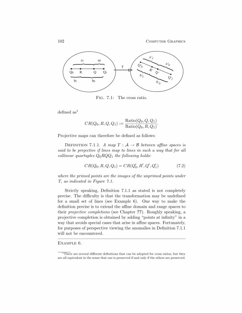
Q0 QR Q1
} }
} }a1
b1 b0
a0 } }} }Q’0
Q’R’
Q’1
a’1
b’0
a’0
b’1
T
102 Computer Graphics
Fig. 7.1: The cross ratio.
defined as1
CR(Q0, R,Q,Q1) :=Ratio(Q0, Q,Q1)
Ratio(Q0, R,Q1).
Projective maps can therefore be defined as follows:
Definition 7.1.1. A map T : A → B between affine spaces issaid to be projective if lines map to lines in such a way that for allcollinear quartuples Q0RQQ1 the following holds:
CR(Q0, R,Q,Q1) = CR(Q′0, R
′, Q′, Q′1) (7.2)
where the primed points are the images of the unprimed points underT, as indicated in Figure 7.1.
Strictly speaking, Definition 7.1.1 as stated is not completelyprecise. The difficulty is that the transformation may be undefinedfor a small set of lines (see Example 6). One way to make thedefinition precise is to extend the affine domain and range spaces totheir projective completions (see Chapter ??). Roughly speaking, aprojective completion is obtained by adding “points at infinity” in away that avoids special cases that arise in affine spaces. Fortunately,for purposes of perspective viewing the anomalies in Definition 7.1.1will not be encountered.
Example 6.
1There are several different definitions that can be adopted for cross ratios, but theyare all equivalent in the sense that one is preserved if and only if the others are preserved.

Q'0C
Q1
R
Q0
Q
Q'1
Q'
R'
α
β
γ
Coordinate-free Geometric Programming II 103
Fig. 7.2: Central projection maps lines to lines and preserves crossratios, hence it is a projective map.
In Section 4.1 it was claimed that perspective projection, alsoknown as central projection, was a projective map. To verifythe claim, we must demonstrate that lines map to lines and thatcross ratios are preserved under central projection. The followingdevelopment is due to Farin [9].
Referring to Figure 7.2, it is clear that lines not containing Cmap to lines under perspective projection. In particular, a line Q0Q1
maps to the line of intersection between the projection plane and theplane containing C, Q0, and Q1. A line through C maps to the pointof intersection between the line and the projection plane. The oneexception to this is for lines through C and parallel to the projectionplane; in fact, the map is not defined for these lines since the lineand the projection plane do not intersect. As mentioned above, fornow we shall simply ignore this small set of anomalous lines.
For those lines that are mapped to lines under central projection,we must show that cross ratios are preserved. We first notice that
Ratio(Q′0, Q
′, Q′1) =
Area(Q′0, Q
′, C)
Area(Q′, Q′1, C)
where Area(A,B,C) denotes the area of the triangle whose verticesare A,B,C. If α = � Q0CR, β = � RCQ, and γ = � QCQ1, then thelaw of sines can be used to show that
Area(Q0, Q,C) =Q0C QC sin(α + β)
2
104 Computer Graphics
implying that CR(Q0, R,Q,Q1) can be written as
CR(Q0, R,Q,Q1) =
¯Q0C QC sin(α + β)QC ¯Q1C sin(γ)
¯Q0C RC sin(α)RC ¯Q1C sin(β + γ)
=sin(α + β) sin(β + γ)
sin(γ) sin(α)(7.3)
Equation 7.3 shows that CR(Q0, R,Q,Q1) depends only on anglesbetween projectors, and not on distances from the points to thecenter of projection. Since the projectors for Q0, R,Q,Q1 are sharedby Q′
0, R′, Q′, Q′
1, we conclude that
CR(Q0, R,Q,Q1) = CR(Q′0, R
′, Q′, Q′1),
thus completing the proof that central projection is a projective map.
Since the cross ratio is a generalization of the simple ratio,every affine transformation is also a projective transformation. It ispossible to show that the composition of two projective maps yields aprojective map (see Exercise 1 on page 118); hence, the compositionof an affine map with a projective map also yields a projective map.
Referring again to Figure 7.1, imagine that the points Q0,R, and Q1 are fixed and that Q is variable. We would like toobtain an expression for Q′ = T (Q) in terms of the fixed pointsand their images Q′
0, R′, and Q′1. To do this, let a0 : a1 =
Ratio(Q0, Q,Q1) and let b0 : b1 = Ratio(Q0, R,Q1); similarly leta′0 : a′1 = Ratio(Q′
0, Q′, Q′
1) and let b′0 : b′1 = Ratio(Q′0, R
′, Q′1),
as shown in Figure 7.1. Since T is projective, Equation 7.2 holds,implying that
a0 : a1
b0 : b1=
a′0 : a′1b′0 : b′1
,
or, equivalently, that
a′0 : a′1 = a0λ0 : a1λ1
where λ0 = b′0/b0, and λ1 = b′1/b1. Thus, Q′ can be expressed as
Q′ =a′0Q
′0 + a′1Q
′1
a′0 + a′1

Coordinate-free Geometric Programming II 105
=(a′0 : a′1)Q
′0 + Q′
1
(a′0 : a′1) + 1
=(a0λ0 : a1λ1)Q
′0 + Q′
1
(a0λ0 : a1λ1) + 1
=a0λ0Q
′0 + a1λ1Q
′1
a0λ0 + a1λ1. (7.4)
Before going further, it is convenient to introduce some simplifyingnotation. Let c0, ..., cn be arbitrary scalars and let Q0, ..., Qn bearbitrary points. We define the bracket notation [·] by
[c0Q0 + · · · + cnQn] :=c0Q0 + · · · + cnQn
c0 + · · · cn.
Using this definition of [·], expressions such as [a�v+ b�w+ cO], whereO is a point can be shown to be
[a�v + b�w + cO] =a
c�v +
a
c�w + O.
Equation 7.4 can now be written more simply as
Q′ = [a0λ0Q′0 + a1λ1Q
′1]. (7.5)
Equation 7.5 states that if Q′0, R
′, and Q′1 are known, then T (Q)
can be computed for any other point Q on the line Q0Q1. In otherwords, T as a map on the line Q0Q1 is completely determined oncethe image of three distinct points is known. Contrast this to thesituation for affine maps: An affine map on a line is completelydetermined once the image of two points is known.
Figure 7.3 illustrates the case of a projective map on a plane. Let(a0, a1, a2) and (b0, b1, b2) be the barycentric coordinates of Q and Rrespectively relative to the triangle Q0Q1Q2, and let (b′0, b
′1, b
′2) be
any numbers such that R′ = [b′0Q′0 + b′1Q
′1 + b′2Q
′2]. In the case that
Q′0, Q
′1, and Q′
2 are affinely independent, these numbers are uniqueup to a scale factor. Using a process similar to the one leading toEquation 7.5, the image of Q under T is given by
T (Q) = T ([a0Q0 + a1Q1 + a2Q2])
= [a0λ0T (Q0) + a1λ1T (Q1) + a2λ2T (Q2)]
= [a0λ0Q′0 + a1λ1Q
′1 + a2λ2Q
′2] (7.6)
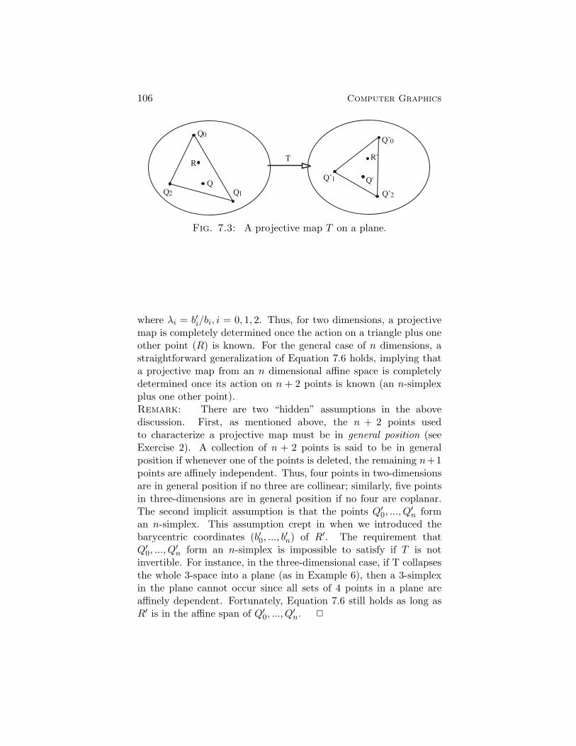
Q1
Q0
Q2
R
Q
Q’0
Q’2
Q’1
R'
Q'
T
106 Computer Graphics
Fig. 7.3: A projective map T on a plane.
where λi = b′i/bi, i = 0, 1, 2. Thus, for two dimensions, a projectivemap is completely determined once the action on a triangle plus oneother point (R) is known. For the general case of n dimensions, astraightforward generalization of Equation 7.6 holds, implying thata projective map from an n dimensional affine space is completelydetermined once its action on n + 2 points is known (an n-simplexplus one other point).Remark: There are two “hidden” assumptions in the abovediscussion. First, as mentioned above, the n + 2 points usedto characterize a projective map must be in general position (seeExercise 2). A collection of n + 2 points is said to be in generalposition if whenever one of the points is deleted, the remaining n+1points are affinely independent. Thus, four points in two-dimensionsare in general position if no three are collinear; similarly, five pointsin three-dimensions are in general position if no four are coplanar.The second implicit assumption is that the points Q′
0, ..., Q′n form
an n-simplex. This assumption crept in when we introduced thebarycentric coordinates (b′0, ..., b
′n) of R′. The requirement that
Q′0, ..., Q
′n form an n-simplex is impossible to satisfy if T is not
invertible. For instance, in the three-dimensional case, if T collapsesthe whole 3-space into a plane (as in Example 6), then a 3-simplexin the plane cannot occur since all sets of 4 points in a plane areaffinely dependent. Fortunately, Equation 7.6 still holds as long asR′ is in the affine span of Q′
0, ..., Q′n. �

Q
P
RT(P)
T(Q)
T(R)
T
Coordinate-free Geometric Programming II 107
Fig. 7.4: The action of a projective map on a line segment.
Even though projective transformations carry points to points, 2
lines to lines, and more generally, hyperplanes to hyperplanes, theydo not preserve the structure of affine spaces (they do, however,preserve the structure of projective spaces). In particular, they donot map vectors to vectors. In fact, it is not possible to extendthe domain of a projective transformation to include vectors. Inan attempt to do so, we might be tempted to offer a definitionsimilar to the one used for affine spaces. That is, suppose Tis a projective transformation and suppose P and Q are pointssuch that �v = P − Q. If we define the action of T on �v byT (�v) = T (P−Q) = T (P )−T (Q) we run into a fundamental difficulty.To be well-formed, the definition of T (�v) should be such that it doesnot matter which pair of points are used as long as their differenceis �v. Unfortunately, the value of T (�v) does depend on the choice ofpoints. An explicit example of this difficulty is shown in Figure 7.4.The point Q is the midpoint of P,R, implying that Q−P = R−Q.However, since T does not map Q to the midpoint of T (P ), T (R),we find that T (Q) − T (P ) �= T (R) − T (Q). Thus, if we used Q andP to compute T (�v), we would arrive at a different result than if wehad used Q and R.
2Actually, as mentioned earlier, some points in the domain can be mapped to pointsat infinity in the range. These points therefore do not have images in the affine rangespace.
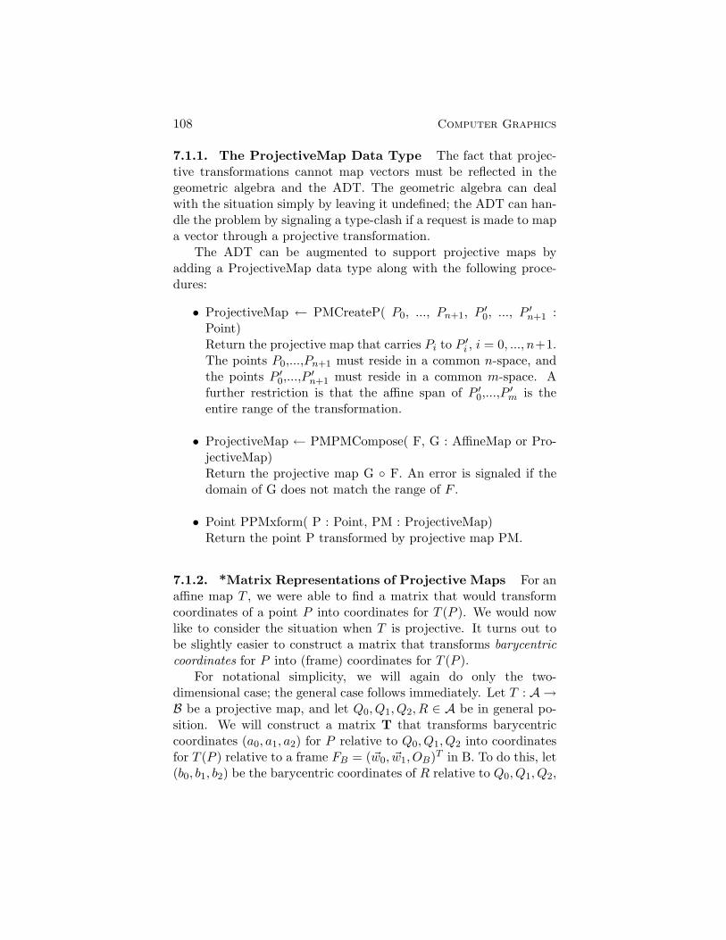
108 Computer Graphics
7.1.1. The ProjectiveMap Data Type The fact that projec-tive transformations cannot map vectors must be reflected in thegeometric algebra and the ADT. The geometric algebra can dealwith the situation simply by leaving it undefined; the ADT can han-dle the problem by signaling a type-clash if a request is made to mapa vector through a projective transformation.
The ADT can be augmented to support projective maps byadding a ProjectiveMap data type along with the following proce-dures:
• ProjectiveMap ← PMCreateP( P0, ..., Pn+1, P ′0, ..., P ′
n+1 :Point)Return the projective map that carries Pi to P ′
i , i = 0, ..., n+1.The points P0,...,Pn+1 must reside in a common n-space, andthe points P ′
0,...,P′n+1 must reside in a common m-space. A
further restriction is that the affine span of P ′0,...,P
′m is the
entire range of the transformation.
• ProjectiveMap ← PMPMCompose( F, G : AffineMap or Pro-jectiveMap)Return the projective map G ◦ F. An error is signaled if thedomain of G does not match the range of F .
• Point PPMxform( P : Point, PM : ProjectiveMap)Return the point P transformed by projective map PM.
7.1.2. *Matrix Representations of Projective Maps For anaffine map T , we were able to find a matrix that would transformcoordinates of a point P into coordinates for T (P ). We would nowlike to consider the situation when T is projective. It turns out tobe slightly easier to construct a matrix that transforms barycentriccoordinates for P into (frame) coordinates for T (P ).
For notational simplicity, we will again do only the two-dimensional case; the general case follows immediately. Let T : A →B be a projective map, and let Q0, Q1, Q2, R ∈ A be in general po-sition. We will construct a matrix T that transforms barycentriccoordinates (a0, a1, a2) for P relative to Q0, Q1, Q2 into coordinatesfor T (P ) relative to a frame FB = (�w0, �w1, OB)T in B. To do this, let(b0, b1, b2) be the barycentric coordinates of R relative to Q0, Q1, Q2,

Coordinate-free Geometric Programming II 109
and let (b′0, b′1, b
′2) be the barycentric coordinates for T (R). Since T
is projective,
T (P ) = T ([a0Q0 + a1Q1 + a2Q2])
= [a0λ0T (Q0) + a1λ1T (Q1) + a2λ2T (Q2)],
where λi = b′i/bi. Thus,
T (P ) =
⎡⎢⎣( a0 a1 a2
)⎛⎜⎝ λ0 0 0
0 λ1 00 0 λ2
⎞⎟⎠
⎛⎜⎝ T (Q0)
T (Q1)T (Q2)
⎞⎟⎠⎤⎥⎦ .
The points T (Q0), T (Q1), T (Q2) possess coordinates qij relativeto FB, so we can write
T (p) =
⎡⎢⎢⎢⎢⎢⎢⎣(
a0 a1 a2
)⎛⎜⎝ λ0 0 0
0 λ1 00 0 λ2
⎞⎟⎠
⎛⎜⎝ q00 q01 1
q10 q11 1q20 q21 1
⎞⎟⎠
︸ ︷︷ ︸T
FB
⎤⎥⎥⎥⎥⎥⎥⎦
(7.7)The matrix T is a representation of T in the following sense.
Given (a0, a1, a2), (p′0, p′1, 1) can be computed from T as follows.
First compute (x0, x1, x2) by matrix multiplication:
(x0 x1 x2 ) = ( a0 a1 a2 )T.
Thus,
T (P ) = [(x0 x1 x2 )FB]
= [x0 �w0 + x1 �w1 + x2OB]
= p′0 �w0 + p′1 �w1 + OB
where p′0 = x0/x2, p′1 = x1/x2. To reiterate, given (a0, a1, a2),(p′0, p
′1, 1) can be computed using a two-step procedure:
(x0 x1 x2 ) := ( a0 a1 a2 )T( p′0 p′1 1 ) := 1
x2(x0 x1 x2 ) .
It is only slightly more difficult to find a matrix T′ thatcarries frame coordinates for p into frame coordinates for T (p) (seeExercise 4 on page 118). Once found, P is transformed through Tby applying the two-step procedure above using T′ in place of T.
Clipping Volume
View box
World
ViewTransform
Screen
sx
sy
sz
dz
ViewFrame
110 Computer Graphics
Fig. 7.5: For perspective viewing the viewing transformation is suchthat the truncated pyramid is mapped to the view box.
7.2. Projective Maps and Perspective Viewing
The idea underlying the creation of hidden surface renderings ofscenes viewed in perspective is essentially the same as was usedin Section 6.2 where a transformation was constructed to map theclipping volume to the view box (see Figure 6.3). The only differencein perspective viewing is that the clipping volume forms a truncatedpyramid instead of a parallelpiped. In other words, to supportperspective viewing, we construct a transformation as indicated inFigure 7.5 that carries the truncated pyramid into the view box. Thistransformation is clearly not affine since parallelism is not preserved.It is, however, projective, meaning that we can fully specify thetransformation by specifying the images of five points in generalposition. Using the five points indicated in Figure 7.6, the desiredtransformation can be constructed as
ViewTransformPM : ProjectiveMap;ViewTransformPM := PMCreateP( P0,P1,P2,P3,C,
P ′0,P
′1,P
′2, P
′3, C
′ : Point)
Once the primitives have been mapped to the view box, thehidden surface algorithms of Chapter 6 can be used without modifi-cation.

World
ViewTransform
Screen
ViewBox
Clipping Volume
P1
P2
P3
P0
C
P'0
P'1
P'2
P'3
C'
Coordinate-free Geometric Programming II 111
Fig. 7.6: The perspective viewing transformation can be specifiedas the one carrying P0,P1,P2,P3,C to P ′
0,P′1,P
′2, P
′3, C
′.
7.3. Normal Vectors and the Dual Space
In many graphics and modeling applications it is convenient tointroduce the idea of a normal vector. For instance, in polygonalmodeling it is common to represent objects by polyhedra where eachvertex is tagged with a normal vector that is used in computingshading information (see Chapter 8). Normal vectors are alsoimportant for ray tracing applications since the surface normaldetermines the direction of a reflected ray, and is one of thedetermining factors in the direction of a refracted ray.
Unfortunately, the term “normal vector” implies that these ob-jects behave just like other vectors. While this is nearly correct, thereare important situations where subtleties can occur. A simplifiedsituation is shown in Figure 7.7 for a hypothetical two-dimensionalpolygonal modeling application. The left portion of Figure 7.7 rep-resents the definition space of a polygonal approximation to a circle.The right portion of the figure is the image of the polygon under theindicated embedding, in this case a non-uniform scaling. Notice thatif the normal vectors are transformed as vectors, then their imagesdo not end up perpendicular to the image of the circle (an ellipse).In fact, they have become more horizontal when they should havebecome more vertical. Such incorrectly transformed normals cancause visual errors in shading and reflection.

FF(v)
v
112 Computer Graphics
Fig. 7.7: Normals transforming as vectors. The gray circle on theleft is being approximated by a set of chords. The vector �v is normalto the circle at the indicated vertex. If �v is mapped through thenon-uniform scaling F , then F (�v) is not perpendicular to the imageof the circle.
One way to understand the problem encountered above isthat vectors were being used to represent two different kinds ofinformation. The first (and fundamental) use of vectors is torepresent parallelism. (Recall that two lines PQ and P ′Q′ areparallel if P−Q is a multiple of P ′−Q′.) The transformation rule forapplying affine maps to vectors was constructed precisely to preserveparallelism. The use of vectors to represent outward pointingnormals is attempting additionally to use vectors to representperpendicularity: an outward pointing normal is perpendicular tothe tangent line (or tangent plane) of the object being modeled.Since perpendicularity is not preserved under affine maps, vectorsfail to be good representatives of tangent lines and tangent planes.
A remedy that is firmly rooted in the fundamentals of geometryis to introduce a new class of objects, classically known as the dualvectors, into the algebra. Intuitively, a dual vector will be usedto directly represent oriented tangent hyperplanes. It will then bepossible to construct a transformation rule for dual vectors thatpreserves tangency. To make these ideas more precise, we must takea short excursion into the concepts of linear functionals and dualspaces.
Warning: The discussion to follow is intended for the purist whois interested in the algebraic details of dual spaces and how theyrelate to normal vectors; for those interested primarily in results,the remainder of this section should probably be skipped, at least

Coordinate-free Geometric Programming II 113
on first reading. The results of this section can be summarized asfollows:
• Dual vectors should be used when representing perpendicular-ity to tangent lines and tangent planes.
• Dual vectors are linear functionals, meaning that a dual vectorφ can be applied to a vector �u to produce a scalar.
• There is a one-to-one association between vectors and dualvectors in a Euclidean space. A vector �v is in association witha dual vector λ if for every vector �w, λ(�w) = �v · �w. If �v andλ are paired in this association, they are called duals of oneanother.
• Dual vectors are represented by the Normal data type in theADT. It is only really necessary to distinguish between a Vectorand a Normal when mapping through affine maps that do notpreserve angles, such as shears and non-uniform scaling.
For the moment, let us leave the realm of affine and Euclideangeometry and work instead in the context of vector spaces. A linearfunctional λ on a vector space V is a map from V into the reals thatsatisfies the linearity condition
λ(α�v + β �w) = αλ(�v) + βλ(�w),
for all �v, �w ∈ V and for all α, β ∈ �. It turns out that the setof all linear functionals on a vector space V itself forms a vectorspace, generally denoted by V∗ (cf. Lang [13]). The vector spaceV∗ of linear functionals is called the dual space of V. To reinforcethe dual nature of the spaces V and V∗, the elements of V are moreaccurately known as primal vectors and the elements of V∗ are calleddual vectors.
An inner product on the vector space can be used to establish anassociation between primal vectors and dual vectors. In particular,using the bracket notation for the inner product, if �v is held fixed, theexpression 〈�v, �u〉 is a linear functional whose argument is �u; that is,λ(�u) := 〈�v, �u〉 is a linear functional on V and is therefore a dual vector(associated with the vector �v). To avoid having to invent a symbolto act as the argument �u, it is more common to write λ := 〈�v, 〉.

114 Computer Graphics
Using this association, we can define the functional 〈�v, 〉 to be thedual of �v. In equation form,
D�v := 〈�v, 〉.
In this form we recognize that D is actually a linear mapping fromV to V∗ since
Dα�v+β �w = αD�v + βD�w.
In fact, D is one-to-one and onto, implying that it is also invertible.The definition of D provides another interpretation of the quantity〈�v, �w〉. By construction, 〈�v, �w〉 = D�v(�w), implying that 〈�v, �w〉 canbe obtained by first dualizing �v, then applying the resulting linearfunctional to �w.
It was mentioned in the introduction to this section that dual vec-tors represent oriented hyperplanes. To see this, notice that D�v(�w)vanishes whenever �w is perpendicular to �v since perpendicularity im-plies that 〈�v, �w〉 = 0. Recall that in a vector space the set of vectorsperpendicular to a fixed vector forms a hyperplane that contains thezero vector. Thus, the linear functional D�v represents an orientedhyperplane through the origin perpendicular to �v. The hyperplaneis oriented because we can distinguish a positive and negative side.The vector �w is on the positive side of the hyperplane if D�v(�w) > 0;it is on the negative side if D�v(�w) < 0.
To translate the above results from vectors in a vector space intoa Euclidean setting, we observe that the freedom of vectors to moveabout in Euclidean space means that a dual vector defines only theorientation of the hyperplane, but does not fix it absolutely in space.The hyperplane can be fixed by specifying a point through whichthe hyperplane must pass. Thus, in a Euclidean space an orientedhyperplane is represented as a point B together with a dual vectorD�n. A point Q is in the positive half-space, negative half-space, oron the boundary if the number D�n(Q − B) is positive, negative, orzero, respectively. This representation for hyperplanes has in factalready been used in Sections 3.9 and 4.3 in conjunction with theSutherland-Hodgman clipping algorithm.
At this point it is not clear that we have gained any new insightfrom the introduction of dual spaces and dual vectors. After all, onecould interpret the above discussion as saying nothing more than aplane is defined by a point P and a vector �v. The advantage of the

Coordinate-free Geometric Programming II 115
dual vector approach is in the determination of how dual vectors,and hence planes and hyperplanes, transform under affine maps.
Let F : A �→ B be an invertible affine map and let �v be a vectorin A.V. We would like to extend the domain of F to include the dualvectors in such a way that perpendicularity is preserved. This goalcan be achieved if we define the action of F on a dual vector D�v as
F (D�v) := D�v ◦ F−1.
To see that perpendicularity is preserved with this definition, let �wbe any non-zero vector in A.V, let �w′ be its image under F ; similarly,let D′
�v be the image of D�v under F . A consequence of the definitionis that D�v(�w) = D′
�v(�w′), since
D�v(�w) = 〈�v, �w〉= 〈�v, F−1 ◦ F �w〉= 〈�v, F−1 �w′〉= D′
�v(�w′).
Thus, if �w lies in the hyperplane defined by D�v (ie, D�v(�w) = 0), then�w′ will lie in the hyperplane defined by D′
�v (ie, D′�v(�w
′) = 0).
Remark: As another remark for the purist, we note that dualvectors, i.e., linear functionals, are an instance of the notion of acovariant tensor. More specifically, dual vectors are covariant tensorsof order one. In general, a covariant tensor of order k is a k-linearmap from a vector space into the reals (cf. [Spivak ’79]); that is,a map T (�v1, ..., �vk) is a covariant tensor of order k if it is linear ineach of its arguments. Tensors are useful objects in fields such asdifferential geometry, continuum mechanics, and relativity theory.Programs designed to solve problems in these areas might thereforebenefit from having tensors included in the algebra and the ADT.�
7.3.1. The Normal Data Type Dual vectors are representedin the geometric ADT by the Normal data type. The routines formanipulation of Normals are:
• Normal ← NCreate( f : Frame; c1, ... , ck : Scalar)Return the Normal whose coordinates in frame f are c1, ... , ck.
116 Computer Graphics
The coordinates of a Normal are defined to be the coordinatesof the vector dual to the normal. Thus, NCreate is equivalentto VDual( VCreate( f , c1, ... , ck)).
• (c1,...,ck : Scalar) ← NCoords( φ : Normal; f : Frame)Return the coordinates of φ relative to f.
• Normal ← VDual( V : Vector)Return the dual to vector V.
• Vector ← NDual( φ : Normal)Return the vector dual to φ.
• Scalar ← NVApply( φ : Normal, V : Vector)Apply φ to V, that is, return φ(V).
• Normal ← NAxform( φ : Normal, T : AffineMap)Return the image of φ under the affine map T ; T is assumedto be invertible.
7.3.2. *Matrix Representations of Dual Vectors Ratherthan representing dual vectors as row matrices as was done for pointsand vectors, dual vectors are most naturally represented as columnmatrices. This is most easily seen by considering the coordinatecomputation of the quantity D�v(�w) = 〈�v, �w〉. If we expand �v and �winto their coordinates relative to a Cartesian frame (�e1, ..., �en,O)T ,we find that
D�v(�w) = 〈v1�e1 + · · · + vn�en, w1�e1 + · · · + wn�en〉.
Bi-linearity is used to rewrite this as
D�v(�w) =∑i,j
viwj〈�ei, �ej〉 (7.8)
Since the basis vectors are ortho-normal, all cross terms (those withi �= j) vanish leaving
D�v(�w) = v1w1 + · · · + vnwn.
Notice that this computation can be written in matrix form as theproduct of a row vector and a column vector:
D�v(�w) = (w1 · · · wn 0 ) ( v1 · · · vn 0 )T
Coordinate-free Geometric Programming II 117
. The row vector is the matrix representation of �w relative to(�e1, ..., �en,O)T , so we can interpret the column vector as the matrixrepresentation of D�v relative to the same frame. Multiplication ofthese matrices corresponds to the application of D�v on �w, and henceresults in the value D�v(�w).
Recall that D was defined as a linear mapping between a vectorspace and its dual space. The fact that a vector �v having coordinates(v1, ..., vn, 0) is represented by the row matrix ( v1 · · · vn 0 ) andhas a dual D�v represented by the column matrix ( v1 · · · vn 0 )T
implies that the mapping D is realized by the matrix transposeoperator. Since the transpose operator is its own inverse, the inverseof D is also realized by the matrix transpose operator.
Given that dual vectors can be represented as column matrices,we now consider the question of how these matrices transform underthe action of affine maps. More precisely, let F : A �→ B be anaffine map whose matrix representation relative to Cartesian framesin A and B is F, and let w and v be the row and column matrices,respectively, that represent �w and D�v relative to the chosen basis.Similarly, let w′ and v′ be the matrix representations of the imagesof �w and D�v under F. With these definitions, it is v′ that we seek.This column vector can be obtained by expanding D�v(�w) in matrixnotation:
D�v(�w) = w v
= w F F−1 v
= w′ F−1 v (7.9)
It was shown earlier that D�v(�w) was invariant under affine maps,implying that D�v(�w) = D′
�v(�w′) = w′ v′. Comparing this with
Equation 7.9 reveals that
w′ F−1 v = w′ v′,
which can be rewritten as
w′(F−1 v − v′
)= 0.
If w′ were a totally arbitrary row vector we could use the non-singularity of F to deduce that
v′ = F−1 v. (7.10)
118 Computer Graphics
There is, however, a problem with taking Equation 7.10 to be thematrix expression for the transformation of dual vectors.3 Considerthe case when F is a translation, meaning that F is of the form givenin Example 5. The inverse matrix is therefore
F−1 =
⎛⎜⎝ 1 0 0
0 1 0−a −b 1
⎞⎟⎠ .
Using this matrix in Equation 7.10 can result in v′ having a non-zerolast component, meaning that it cannot be used as the representationof a dual vector. The solution to this dilemma is hidden in the factthat w′ is not totally arbitrary because its last component must bezero. This means that all but the last component of v′ must agreewith F−1 v, but the last component can, without loss of generality,be chosen to be zero. This choice can be forced by introducing a(n+ 1)× (n+ 1) matrix Z that contains all zero elements except forones on the first n diagonals. We therefore take as our transformationrule for dual vectors the matrix expression
v′ = Z F−1 v. (7.11)
One further caveat is in order: Equation 7.11 is only valid whencoordinates are expressed relative to Cartesian frames. If coordinatesare expressed in a non-Cartesian frame, the transformation rulebecomes slightly more complicated. The simplification occurs forCartesian frames because the cross terms in Equation 7.8 areguaranteed to vanish. We leave the generalization to arbitrary framesas an exercise.
Exercises
1. Show that the composition of two projective maps is projective.
2. What goes wrong if the pre-image points used to define aprojective map are not in general position?
3. Show that planes map to planes under projective maps.
4. Extend the results of Section 7.1.2 to determine a matrixT′ that carries frame coordinates for a point P into framecoordinates for the point T (P ), where T is a projective map.
3Thanks to Richard Bartels for pointing this out.

Coordinate-free Geometric Programming II 119
5. Derive the matrix transformation rule for dual vectors whenarbitrary (i.e., non Cartesian) frames in A and B are chosen.

120 Computer Graphics
Chapter 8
Color and Shading
To create images with smoothly varying, physically plausible, colorvariations, we must develop models that approximate the interactionof light with surfaces. Before developing these lighting models, weshall look more closely at what is meant by “color” by taking a shortdetour through the basics of tri-stimulus color theory.
8.1. Tri-Stimulus Color Theory
Consider the artificially simple situation of a human observer lookingat a single colored light source. We know from elementary physicsthat the light source can be physically characterized by an emis-sion spectrum I(λ) that assigns an intensity of emission to eachwavelength λ of the electromagnetic spectrum. A device such as aspectrophotometer could be used to physically measure the emissionspectrum from the light source. The human observer on the otherhand would describe the perceived color of the light, perhaps usingwords such as “bluish yellow” or “light green”. The key word here isperceives: whereas nature generates spectra, humans perceive color.
The distinction between spectra and color has been made strik-ingly clear through experiments in color theory. It is possible forinstance to present two very different spectra to an observer withoutthe observer being able to tell them apart. (Two distinct spectrathat are perceived as being identical are called metamers.) Theimplication of such experiments is that the number of perceivablecolors is much smaller than the number of spectra. This implicationis corroborated by biological evidence. A (normal) human retinapossesses three different types of color receptors. Roughly speaking,these receptors respond most strongly to long wavelengths, medium
121

122 Computer Graphics
Fig. 8.1: Response curves for the short (S), medium (M), and long(L) wavelength human color receptors.
wavelengths, and short wavelengths, of light respectively. The ac-tivity levels for each of the receptors for a variety of wavelengthshave been measured, resulting in the response curves shown in Fig-ure 8.1. Since the long wavelength receptor peaks in the red portionof the spectrum, it is commonly referred to as the red receptor. Themedium and short wavelength receptors are commonly known as thegreen and blue receptors, respectively.
Tri-stimulus color theory attempts to explain the associationbetween spectra and color by modeling the low-level or “early”human vision system as a linear mapping V : Λ → C, where Λis the (infinite dimensional) vector space of continuous functions ofwavelength, and C is a three-dimensional vector space called colorspace. Specifically, tri-stimulus theory states that V is given by givenby
V (I(λ)) = �c = ��� + m�m + s�s. (8.1)
where the vectors ��, �m,�s form a basis for C. The scalars �, m, and sindicate the level of activity of each of the the three color receptorsin response to stimulation by the spectrum I(λ); they are computed

Lighting Models and Color 123
according to
� =
∫ ∞
−∞L(λ)I(λ)dλ
m =
∫ ∞
−∞M(λ)I(λ)dλ
s =
∫ ∞
−∞S(λ)I(λ)dλ
where L, M , and S are the receptor response functions of Figure 8.1.Since the range of V has a smaller dimension than its domain, it is
necessarily a many-to-one mapping, thereby offering an explanationfor the existence of metamers.
Although tri-stimulus theory is adequate for many computergraphics tasks, it is not adequate for all purposes since there aremany phenomena that the theory fails to predict. For instance, wehave all noticed that the color of a piece of fabric or a paint chip seemsto change depending on what other colors are nearby. Theories thatadequately explain such effects are still an active area of research.
8.1.1. Reproducing Spectral Responses with Frame BuffersA natural problem to consider in the context of computer graphicsis:
Given: A spectrum I(λ).
Find: r, g, b values to store in a frame buffer so that thecolor viewed on the screen evokes the same perceptualresponse as I(λ).
To examine this question more closely, we first note that thespecific r, g, b values will clearly depend on the specifics of themonitor. In particular, it will be critical to know the emission spectraR(λ), G(λ) and B(λ) of each of the red, green, and blue phosphors,respectively. Assuming the monitor has been gamma corrected, thesynthesized spectrum I ′(λ) appearing on the monitor correspondingto a pixel value (r, g, b) is
I ′(λ) = rR(λ) + gG(λ) + bB(λ). (8.2)
Given I(λ) we wish to compute (r, g, b) such that I(λ) and I ′(λ)are metamers; that is, we require
V (I(λ)) = �c = V (I ′(λ)). (8.3)
124 Computer Graphics
To solve the problem, we first note that as a consequence of thelinearity of integration, the mapping V is a linear transformation,meaning that for any two spectra X(λ) and Y (λ), and for any scalarsa and b,
V (aX(λ) + bY (λ)) = aV (X(λ)) + aV (Y (λ)).
Linearity of V implies that
V (I ′(λ)) = rV (R(λ)) + gV (G(λ)) + bV (B(λ))
= r�r + g�g + b�b,
where the vectors �r, �g, and �b are V (R(λ)), V (G(λ)) and V (B(λ)),respectively. Substituting Equations 8.4 and 8.1 into Equation 8.3,we find that
�c = r�r + g�g + b�b = ��� + m�m + s�m. (8.4)
In vector space terms, Equation 8.4 states that (r, g, b) are thecoordinates of �c in the basis (�r,�g,�b), and (�,m, s) are the coordinatesfor �c in the basis (��, �m,�s). We therefore recognize the calculation of(r, g, b) from (�,m, s) as a simple change of coordinates; hence theremust exist a 3 × 3 matrix A such that(
r g b)
=(
� m s)A.
In fact, it can be shown that (see Exercise 1 on page 134)
A =
⎛⎜⎝ αRL αRM αRS
αGL αGM αGS
αBL αBM αBS
⎞⎟⎠
−1
(8.5)
where
αXY =
∫ ∞
−∞X(λ)Y (λ)dλ
X ∈ {R,G,B}, Y ∈ {L,M,S}.The change of basis matrix A can be computed once the emission
spectra are known for the monitor on which the input spectra are tobe reproduced. Once A is computed, the (r, g, b) triple correspondingto a spectrum I(λ) can be found by first computing (�,m, s), thenmultiplying by A to obtain (r, g, b).
Lighting Models and Color 125
Our coordinate-free machinery can be used to explain the aboveprocess as follows. The human visual system corresponds to thebasis (��, �m,�s) for the color space C since coordinates relative tothis basis indicate the level of activity in human color receptors.Each monitor corresponds to a different basis (�r,�g,�b), where therelationship between the “monitor basis” and the “human basis”depends on the phosphor emission spectra of the monitor. Themonitor basis is therefore the color equivalent of the (spatial) deviceframe imposed on screen space.
8.1.2. The CIE Color System An organization called theCommision Internationale de l’Eclairage (CIE) has devised a colorreproduction process that is somewhat more accurate than the pro-cess above (inaccuracies in the above process are due to deficienciesin the tri-stimulus theory). Rather than computing (r, g, b) by firstcomputing (�,m, s) from the spectrum, the CIE developed a twostep process wherein the coordinates (x, y, z) of V (I(λ)) relative toan agreed upon standard basis (�x, �y, �z) for color space are first com-puted. The (r, g, b) coordinates appropriate for a particular monitorare computed from (x, y, z) using a change of basis matrix.
Increased accuracy was achieved by the CIE by experimentallydetermining lookup tables that represent the mapping from spectrato (x, y, z). This was done by presenting human observers withcolored lights corresponding to large number of different wavelengths.For each wavelength, the subjects were asked to adjust the red, green,and blue values on a high quality color monitor until the color onthe monitor matched the color of the spectrum. This resulted in atable that mapped directly from spectra to (r, g, b) for that particularmonitor. The effects of the monitor were then factored out byperforming a change of coordinates from (�r,�g,�b) to (�x, �y, �z). Thefamous CIE chromaticity diagram corresponds to the colors lying onthe plane
x�x + y�y + z�z, x + y + z = 1.
8.2. Lighting Models
The problem to be addressed in this section can be stated roughlyas follows:
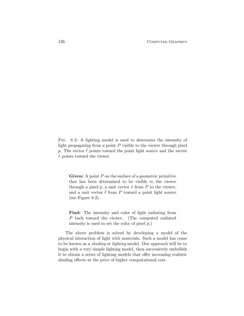
126 Computer Graphics
Fig. 8.2: A lighting model is used to determine the intensity oflight propagating from a point P visible to the viewer through pixelp. The vector � points toward the point light source and the vectorv points toward the viewer.
Given: A point P on the surface of a geometric primitivethat has been determined to be visible to the viewerthrough a pixel p, a unit vector v from P to the viewer,and a unit vector � from P toward a point light source(see Figure 8.2).
Find: The intensity and color of light radiating fromP back toward the viewer. (The computed radiatedintensity is used to set the color of pixel p.)
The above problem is solved by developing a model of thephysical interaction of light with materials. Such a model has cometo be known as a shading or lighting model. Our approach will be tobegin with a very simple lighting model, then successively embellishit to obtain a series of lighting models that offer increasing realisticshading effects at the price of higher computational cost.
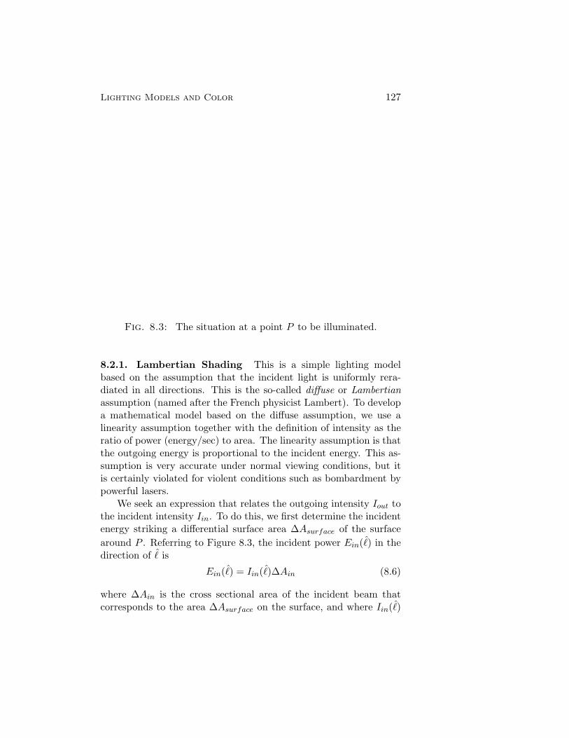
Lighting Models and Color 127
Fig. 8.3: The situation at a point P to be illuminated.
8.2.1. Lambertian Shading This is a simple lighting modelbased on the assumption that the incident light is uniformly rera-diated in all directions. This is the so-called diffuse or Lambertianassumption (named after the French physicist Lambert). To developa mathematical model based on the diffuse assumption, we use alinearity assumption together with the definition of intensity as theratio of power (energy/sec) to area. The linearity assumption is thatthe outgoing energy is proportional to the incident energy. This as-sumption is very accurate under normal viewing conditions, but itis certainly violated for violent conditions such as bombardment bypowerful lasers.
We seek an expression that relates the outgoing intensity Iout tothe incident intensity Iin. To do this, we first determine the incidentenergy striking a differential surface area ∆Asurface of the surface
around P . Referring to Figure 8.3, the incident power Ein(�) in thedirection of � is
Ein(�) = Iin(�)∆Ain (8.6)
where ∆Ain is the cross sectional area of the incident beam thatcorresponds to the area ∆Asurface on the surface, and where Iin(�)
128 Computer Graphics
denotes the incident intensity arriving from direction �. Using thelinearity assumption, we write
Eout(v) = φ(v, �)Ein(�) (8.7)
where φ(v, �) is the constant of proportionality that relates theincoming power from the direction � to the outgoing power in thedirection of v; it is a property of the material, characterizing howenergy is reflected off the surface. Combining Equations 8.6 and 8.7and using the relation
Iout(v) =Eout(v)
∆Aout,
we find that
Iout(v) = φ(v, �)Iin(�)∆Ain
∆Aout(8.8)
= φ(v, �)Iin(�)∆Ain
∆Asurface
∆Asurface
∆Aout. (8.9)
Referring to Figure 8.3, the ratio of ∆Ain to ∆Asurface is cos θin;similarly, the ratio of ∆Aout to ∆Asurface is cos θout, implying that
Iout(v) = φ(v, �)Iin(�)cos θincos θout
0 ≤ θin, θout ≤ π/2. (8.10)
The diffuse reflection assumption states that Iout(v) is independentof v, meaning that
φ(v, �) = ρ(v, �) cos θout. (8.11)
The function ρ(v, �) is called the bidirectional reflectance. Thebidirectional reflectance for a diffusely reflecting surface is assumedto be a constant kd. Using Equation 8.11, Equation 8.10 can berewritten as
Iout(v) = kdIin(�)(� · n)+ (8.12)
where (x)+ is defined to be x if x ≥ 0, and zero otherwise.Equation 8.12 is the diffuse lighting model. As a consequence
of the linearity assumption, multiple light sources can be modeledsimply by summing the contributions from each light source. Noticehowever that Iin(�) as used in Equation 8.12 is the intensity of the
Lighting Models and Color 129
light source as measured at P . The conservation of energy principlefrom physics predicts that the intensity of a point light source obeysthe inverse square law – the intensity falls off as one over the distancefrom the source squared. Thus,
Iin(�) =I0r2
where r is the distance from the light source to P , and I0 is theintensity of the source as measured at unit distance. Althoughthe inverse square law is physically accurate for a point source, thelighting effects produced using it are extremely harsh. One reason forthe harshness is that true point light sources are never encounteredin everyday experience. The lighting effects can be improved in anumber of ways. The most physically justified method is to modellight sources with finite extent by integrating Equation 8.12 overthe area of the light source. This is in fact the approach taken bya number of global illumination methods that will be discussed inChapter ??. A much less expensive (empirical) approximation is tomodel the intensity fall off as
Iin(�) =I0
γ + r
where γ is a constant associated with the light source.It should also be noted that Iout(v) is the intensity leaving P
toward the viewer. The pixel p through which P is visible shouldbe set to the intensity as measured at p. Thus, strictly speaking, pshould be set to an intensity Iout(v)/d
2, where d is the distance fromP to p. Once again, this fast decay in intensity produces illuminationeffects that are too harsh. It is therefore very common in graphicsto simply ignore the intensity fall off between P and p.
Colored light sources reflecting off colored surfaces are mostaccurately modeled by treating Iin, Iout, and kd in Equation 8.12 asfunctions of wavelength. Once the final spectrum I(λ) is determined,it can be mapped to a color by applying the mapping V given inEquation 8.1. The physically correct method is therefore to performall calculations in Λ, then map to C to obtain a color.
In computer graphics, however, it is traditional to handle colorby maintaining red, green, and blue color components separately.For example, color light sources are typically characterized by their

130 Computer Graphics
red, green, and blue intensities; that is, a light source with spectrumI(λ) is most often represented by the (r, g, b) coordinates of V (I(λ)).The diffuse reflectances of colored materials are similarly character-ized by three coefficients (kd,red, kd,green, kd,blue). For instance, a pre-dominantly red material would be characterized by a value of kd,rednear one, and values of kd,green and kd,blue near zero.
The approach traditionally taken in computer graphics is essen-tially to perform all calculations in C rather than in Λ. There area number of difficulties with this (virtually universal) approach. Forinstance, the physically correct color corresponding to the calcula-tion I1(λ) + k(λ) ∗ I2(λ) in Λ is
V (I1(λ) + k(λ) ∗ I2(λ)) = V (I1(λ)) + V (k(λ) ∗ I2(λ)). (8.13)
The component-wise color computed by the usual computer graphicsapproach can be formally described by
V (I1(λ)) + V (k(λ)) ⊗ V (I2(λ)), (8.14)
where ⊗ is defined follows: if �x = rx�r + gx�g + bx�b and �y =ry�r + gy�g + by�b, then
�x⊗ �y = rxry�r + gxgy�g + bxby�b.
The two results given in Equations 8.13 and 8.14 will, in general,not be equal since V does not preserve multiplication of functions.More precisely, if X(λ), Y (λ) ∈ Λ, V (X(λ)∗Y (λ)) is not, in general,equal to V (X(λ)) ⊗ V (Y (λ)).
A number of groups, led primarily by Cornell University, havebeen advocating the physically correct approach of performing light-ing calculations in Λ, using for instance, piecewise linear approx-imations of functions. Unfortunately, the approach is still notwidespread. In the remainder of this chapter, we succumb to thesin of performing calculations in C using component-wise computa-tions for the red, green, and blue color coordinates.
Putting all the pieces together, we set the color components ofpixel p to
Iout,c(v) =∑
light source i
ρc(v, �i)Ii0,c
γi + ri(�i · n)+ (8.15)
Lighting Models and Color 131
c ∈ {red, green,blue}
where ρc(v, �) = kd,c.Finally, we mention another simple type of light source called
a directional light source. A directional source models a distanntpoint light source such as the sun. Unlike a point light source wherethe vector � depends on the point P being illuminated, directionallight sources are modeled using a vector � that does not depend onP , thus capturing the fact that incoming rays from the light areparallel. Another difference is that since the light rays are parallel,there is no intensity fall off with distance.
8.2.2. Ambient Lighting The images produced by the lightingmodel of Equation 8.15 are still rather harsh. One reason for theharshness is that only direct illumination is modeled – there is noaccount taken of indirect illumination that is so often present innatural environments. In an office, for instance, the floor underneatha desk receives some light even though the area is not directlyilluminated by a light source. The global illumination algorithms inChapter ?? are specifically designed to accurately model indirectillumination. A reasonably effective but very simple empiricalmethod is to model only ambient illumination. Ambient illuminationrefers to a completely uniform level of light that is visible to allsurfaces. The light model can be augmented to including ambientillumination by replacing Equation 8.15 with
Iout,c(v) = ρa,cIa,c +∑
light source i
ρc(v, �i)Ii0,c
γi + ri(�i · n)+ (8.16)
c ∈ {red, green,blue}
where• ρc(v, �) = kd,c is the diffuse bidirectional reflectance.
• ρa,c is the ambient bidirectional reflectance. It is commonto assume that the material diffusely reflects the ambientillumination, meaning that ρa,c = kd,c.
• Ia,c is the intensity of the ambient illumination.
132 Computer Graphics
8.2.3. Specular Reflection Specular (shiny) surfaces are notmodeled well by diffuse reflection since they exhibit preferentialreradiation. The observed intensity of a point P on a near-perfectmirror surface, for instance, depends on the position of the viewerrelative to the light source. If the viewer is positioned so that thereflection of the light source is visible at P , the intensity at P appearsto be very bright. The variation of the intensity of a point with theposition of a viewer is not an effect captured by the diffuse model.
Torrance and Sparrow developed a model of specularly reflectingsurfaces by treating the surface as being composed of microscopicperfectly reflecting flat facets called microfacets [18, 19]. Themicrofacets are assumed to have normal vectors oriented in adistribution about the macro surface normal n, thereby modeling themicroscopic flaws that prevent real materials from being perfectlymirror-like. Torrance and Sparrow show that the bidirectionalreflectance function for this model of specular reflection is of theform
ρs(v, �) = σDG
(n · v)(n · �)where
• σ is a constant.
• D is a function describing the distribution of microfacetnormals.
• G is a self-shadowing factor, accounting for the shadowing ofsome microfacets by other microfacets.
Although the Torrance-Sparrow model was known in the physicsliterature in the late 60’s, Phong Bui-Tuong, working at the Univer-sity of Utah in the computer graphics laboratory in the mid ’70s,independently developed an empirical model of specular reflectionthat is qualitatively very similar to the Torrance-Sparrow model. Inparticular, Bui-Tuong used a model of specularity that is equivalentto the bidirectional reflectance
ρs,c(v, �) = ks,c(r · v)p+(n · �)+
, c ∈ {red, green,blue}
where r is a unit vector pointing in the mirror direction as shown inFigure 8.4. This model of specular reflection has come to be known

Lighting Models and Color 133
Fig. 8.4: The quantities necessary for the Phong lighting model.
as the Phong lighting model. The maximum intensity occurs whenthe viewing direction v aligns with the mirror direction r, since theterm (r ·v)p+ reaches its maximum value of one. The number p, calledthe Phong exponent, controls the rate at which a specular reflectionfalls off as v moves away from r, thereby controlling the width ofspecular highlights as seen on the surface. Small values of p causebroad highlights whereas large values of p create narrow, sharplyfocused highlights. The Phong exponent then roughly correspondsto the “shinyness” of the surface, with large values of p correspondingto very shiny materials. In terms of the Torrance-Sparrow microfacetmodel, p corresponds to the width of the distribution of microfacetnormals about the macro surface normal n.
The values ks,red, ks,green, ks,blue characterize the degree to whichthe surface specularly reflects in each of the color channels. Thesevalues effectively control the color of specular highlights.
A lighting model incorporating the effects of ambient, diffuse,and the Phong model of specularity is given by
Iout,c(v) = ρa,cIa,c +∑
light source i
ρc(v, �i)Ii0,c
γi + ri(�i · n)+ (8.17)
134 Computer Graphics
where
ρc(v, �i) = kd,c + ks,c(ri · v)p+(n · �i)+
.
Exercises
1. Prove that the matrix A that changes coordinates relative to(��, �m,�s) to coordinates relative to (�r,�g,�b) has the form givenin Equation 8.5.
2. Develop a formula for computing the mirror direction vector rfrom n, and �.

Lighting Models and Color 135
References
[1] W. Bouknight. A procedure for generation of three-dimensional half-toned computer graphics representations. Communications of theACM, 13(9):527–536, September 1970.
[2] W. Bouknight and K. Kelly. An algorithm for producing half-tonecomputer graphics presentations with shadows and movable lightsources. SJCC, pages 1–10, 1970.
[3] J. E. Bresenham. Algorithm for computer control of a digital plotter.IBM Systems Journal, 4(1):25–30, 1965.
[4] E. Catmull. A Subdivision Algorithm for Computer Display of CurvedSurfaces. PhD thesis, Computer Science Department, University ofUtah, December 1974.
[5] E. Catmull. A tutorial on compensation tables. In Proceedings ofSIGGRAPH, pages 279–285, 1979.
[6] C. de Boor. B-form basics. In G. Farin, editor, Geometric Modeling:Algorithms and New Trends, pages 131–148. 1987.
[7] Manfred P. do Carmo. Differential Geometry of Curves and Surfaces.Prentice-Hall, Inc., Englewood Cliffs, New Jersey, 1976.
[8] C. Dodson and T. Poston. Tensor Geometry: The GeometricViewpoint and its Uses. Pitman, London, 1979.
[9] G. Farin. Curves and Surfaces for Computer Aided Geometric Design.Addison-Wesley, New York, second edition edition, 1990.
[10] F. Flohr and F. Raith. Affine and Euclidean geometry. In H. Behnke,F. Bachmann, K. Fladt, and H. Kunle, editors, Fundamentals ofMathematics, Volume II, pages 293–383. MIT Press, 1974.
[11] J. Foley, A. van Dam, S. Feiner, and J. Hughes. Computer Graphics,Princples and Practice. Addison-Wesley, New York, 1990.
[12] R. Goldman. Vector geometry: A coordinate-free approach. SiggraphCourse Notes, Course No. 19, 1987.
[13] Serge Lang. Algebra. Addison-Wesley, Redwood City, California,second edition, 1984.
[14] M. O’Nan. Linear Algebra. Harcourt Brace Jovanovich, Inc., NewYork, second edition edition, 1976.
[15] M. L. V. Pitteway. Algorithm for drawing ellipses or hyperbolae witha digital plotter. Computer Journal, 10(3):282–289, 1967.
[16] R. Sproull and I. Sutherland. A clipping divider. In FJCC, pages765–775. Thompson Books, Washington, D.C., 1968.
[17] I. E. Sutherland and G. W. Hodgman. Reentrant polygon clipping.Communications of the ACM, 17(1):32–42, 1974.
[18] K. Torrance and E. Sparrow. Theory of off-specular reflection fromroughened surfaces. Journal of the Optical Society of America,57(9):1105–1114, 1967.
136 Computer Graphics
[19] K. Torrance, E. Sparrow, and R. Birkebak. Polarization, directionaldistributional, and off-specular peak phenomena in light reflectedfrom roughened surfaces. Journal of the Optical Society of America,56(7):916–925, 1966.
[20] J. Warnock. A hidden-surface algorithm for computer generated half-tone pictures. Computer Science Department TR 4-15, NTIS AD-753671, University of Utah, 1969.
[21] G. Watkins. A real-time visible surface algorithm. Computer ScienceDepartment UTEC-CSc-70-101, NTIS AD-762 004, University ofUtah, June 1970.
[22] K. Weiler and P. Atherton. Hidden surface removal using polygonarea sorting. In Proceedings of SIGGRAPH, pages 214–??, 1977.
[23] H. Weyl. Space, Time, and Matter. Methuen & Co., London, 1922.Translated from German by H. Brose.
[24] C. Wylie, G. Romney, D. Evans, and A. Erdahl. Halftone perspectivedrawings by computer. FJCC 1967, pages 49–58, 1967.


