Ocean Engineering 64 (2013) 161–173

Contents lists available at SciVerse ScienceDirect

Ocean Engineering

0029-80

http://d

n Corr

E-m

journal homepage: www.elsevier.com/locate/oceaneng

Three-dimensional dynamics of long pipes towed underwater.Part 2 Linear dynamics

M. Kheiri a, M.P. Paıdoussis a,n, M. Amabili a, B.I. Epureanu b

a Department of Mechanical Engineering, McGill University, 817 Sherbrooke Street West, Montreal, QC, Canada H3A 0C3b Department of Mechanical Engineering, University of Michigan, Ann Arbor, MI, USA

a r t i c l e i n f o

Available online 13 March 2013

Keywords:

Finite difference method

Pinned–pinned pipes

Towed pipes

Divergence

Flutter

18/$ - see front matter & 2013 Elsevier Ltd. A

x.doi.org/10.1016/j.oceaneng.2013.01.007

esponding author. Tel.: þ1 514 398 6294; fax

ail address: michael.paidoussis@mcgill.ca (M.

a b s t r a c t

In this paper, a method of solution based on a finite difference scheme is developed, via which the

partial differential equations of motion and boundary conditions, presented in Part 1, are converted into

a set of first-order ODEs which are then solved numerically. The mathematical model is validated by

considering some simplifications which enable us to compare the numerical results with the results of

short pipes simply supported at both ends (pinned–pinned) and subjected to axial flow. A typical

Argand diagram is then presented for a long pipe (L ¼ 2000 m) which shows the evolution of lowest

three eigenfrequencies of the system as a function of nondimensional flow velocity (towing speed).

For the same pipe, the deformation and time-trace diagrams at different values of flow velocity are also

given. The results show clearly that a long pipe towed underwater may lose stability by divergence and

at higher flow velocities by flutter; the deformation is confined to a small segment of the pipe, close to

the downstream end. Some numerical comparisons are also presented in which the effects of cable

stiffness and the skin friction coefficient on the onset of instabilities are studied.

& 2013 Elsevier Ltd. All rights reserved.

1. Introduction

In Part 1 of this two-part study, the equations of motion for thedynamics of long pipes (cylinders) towed underwater have beenderived. In fact, these equations can be used to study thedynamics of both long and short pipes subjected to axial flow,since no limiting simplification has been made on the flexuralrigidity of the pipe, contrary to some other studies in which, forlong pipes, the flexural rigidity of the body has been neglected(e.g., Triantafyllou and Chryssostomidis, 1985) or only partly beentaken into account (e.g., Dowling, 1988).

Interest in the dynamics of very slender cylinders, where thelength-to-diameter ratio, L=D, is of order 102 or even 105,subjected to axial flow may also be found in some of the earliestwork carried out for possible application to submarine antennasand hydrophone arrays (e.g., Ortloff and Ives, 1969; Pao, 1970;Lee, 1981). In these analyses, which unfortunately were madebased on the erroneous version of equations of motion proposedby Paıdoussis (1966), and not the corrected ones (Paıdoussis,1973), they found a different stability behaviour for long cylindersfrom that of short ones.

ll rights reserved.

: þ1 514 398 7365.

P. Paıdoussis).

Recently, in a paper by de Langre et al. (2007), the stability of athin flexible cylinder subjected to axial flow and fixed at theupstream end has been considered. Contrary to previous predic-tions made via simplified models (Dowling, 1988; Triantafyllouand Chryssostomidis, 1985), they found that flutter may arise forvery long cylinders if the free downstream end of the cylinder iswell-streamlined. They also found a limit regime in which theinstability characteristics of the system are not affected by thelength of the cylinder, and the cylinder deformation is confined toa finite region close to the downstream end.

A number of experiments were conducted (Paıdoussis, 1968)with relatively short (L=DC20) flexible cylinders held in flow bya length of string attached to their upstream end. Later, Ni andHansen (1978) studied experimentally the flow-induced lateralmotions of a flexible tube in axial flow; the flexible tube was veryslender (L=DC500) and approximately neutrally buoyant, and itwas fixed at the upstream end and free at the downstream end.A set of experiments were also carried out by Sudarsan et al.(1997) to study the hydroelastic instability of flexible slendercylinders towed underwater. These experiments were conductedin a towing tank, and the models were with length-to-diameterratios of 50 and 150. Generally, in the above-mentioned experi-ments divergence and flutter have been observed; moreover, inthe case of very slender cylinders, the deformation seems to becentered particularly in the region close to the downstream end ofthe cylinders.

0.001

0.002

M. Kheiri et al. / Ocean Engineering 64 (2013) 161–173162

In this paper, a finite difference scheme is used to spatiallydiscretize the linearized unsteady equations of motion. Theresultant set of time-domain ODEs are solved by using DIVPAGroutine of Fortran IMSL library. Then, a simplified version of theequations which mimics the dynamical behaviour of short simplysupported (pinned–pinned) pipes in axial flow is used to validatethe present model. Finally, in the last part of this paper, thenumerical results for the dynamics of long pipes flexibly con-nected to a towing vessel at the upstream end and to a trailingvessel at the downstream end are presented.

It is emphasized that the model considered here, involvinglong pipes towed underwater and subject to realistic nonclassicalboundary conditions, is presented for the first time. In thenumerical solutions presented, the effect of various systemparameters is examined for the first time. Moreover, this paperpresents numerical solutions for both short and long pipes,allowing the reader to understand the dynamical features of bothsystems, side by side.

0 0.2 0.4 0.6 0.8 1

-0.003

-0.002

-0.001

0

2. The method of solution

In this section, the method of solution for the unsteadyequations of motion for cases with only axial flow (no cross-current) is discussed. Although equations for both the steady state(related to the effect of a cross-current) and for unsteady self-excited motions have been derived in Part 1, we are not going topresent any numerical solutions here for the steady current-induced deformation, since this is not the aim of this study. Thedynamics in the presence of a cross-flow is the subject of anotherpaper, currently under preparation.

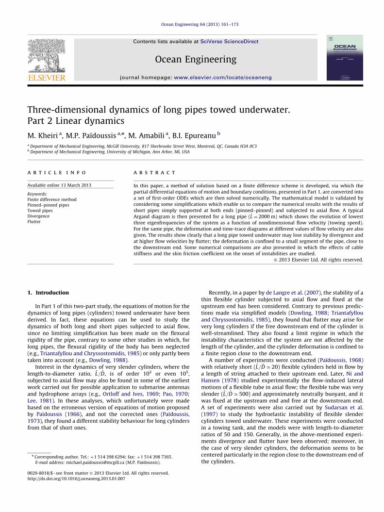
Fig. 2. Typical results showing (a) the shape of a ‘‘short pipe’’ with very stiff end-

springs at different time instants and (b) the time trace of the pipe mid-point;

Ux ¼ 0:70.

2.1. The unsteady equations of motion

With no cross-current (Uz ¼ 0), there is no steady-state defor-mation in the z-direction. In this case the y- and z-directionequations, as given in Part 1, become identical, and the dynamicsof the system can be studied by solving one of them. The equationof motion in the z-direction can be written as

a4 @4w

@x4þa2ðU2

x�T Þ@2w

@x2þ2ab1=2Ux

@2w

@x@tþ

1

2aU2

xecf@w

@x

þ1

2Uxecfb

1=2þ

1

2ecdb

1=2� �

@w

@tþ@2w

@t2¼ 0, ð1Þ

in which all quantities are nondimensional. Here w is the dis-placement in the z-direction, x the longitudinal coordinate, and ea measure of the slenderness ratio defined as e¼ ‘=D where‘ ¼ ½ðpDÞ2L�1=3; t represents time, and L and D are the length andthe diameter of the pipe, respectively; Ux the axial flow velocity(tow speed), b the ratio of the fluid mass to the total mass (fluidand structure), cf the frictional drag coefficient, cd the zero-flownormal coefficient, and a a coefficient used for normalizing thelongitudinal coordinate; T the steady tension in the pipe, whichcan be found in the dimensional form in Eq. (17) of Part 1.

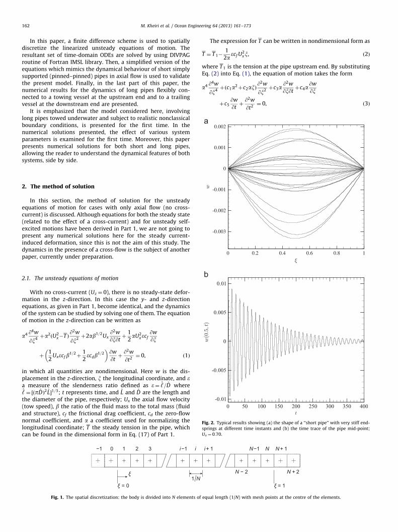
−1 0 1 2 3 i−1 i

ξ = 0

ξ1 N

Fig. 1. The spatial discretization: the body is divided into N elements of

The expression for T can be written in nondimensional form as

T ¼ T 1�1

2a ecf U2xx, ð2Þ

where T 1 is the tension at the pipe upstream end. By substitutingEq. (2) into Eq. (1), the equation of motion takes the form

a4 @4w

@x4þðc1a2þc2axÞ

@2w

@x2þc3a

@2w

@x@tþc4a

@w

@x

þc5@w

@tþ@2w

@t2¼ 0, ð3Þ

i + 1

N − 2

N−1 N N + 1

N + 2

ξ = 1

equal length (1/N) with mesh points at the centre of the elements.

M. Kheiri et al. / Ocean Engineering 64 (2013) 161–173 163

where c1 ¼U2x�T 1, c2 ¼

12ecf U2

x , c3 ¼ 2b1=2Ux, c4 ¼ c2 and c5 ¼12 Uxecfb

1=2þ1

2ecdb1=2.

The boundary conditions can be simplified to

@2w

@x2

�����x ¼ 0

¼@2w

@x2

�����x ¼ 1

¼ 0 ð4Þ

and

a3 @3w

@x3þaað1Þ1,z

@w

@xþað1Þ3,zw�að1Þ4,z

!�����x ¼ 0

¼ 0,

a3 @3w

@x3þaað2Þ1,z

@w

@xþað2Þ3,zw�að2Þ4,z

!�����x ¼ 1

¼ 0: ð5Þ

Following Iwatsubo et al. (1973), Sugiyama and Kawagoe(1975) and Sugiyama et al. (1976), we use the central finitedifference method to spatially discretize the equation of motionand the boundary conditions. In order to apply the method, thebody is assumed to be divided into N elements. As seen in Fig. 1,

0 0.2 0.4 0.6 0.8 1

0.05

0.1

0.15

0.2

0 10 20 30 40 50

0.05

0.1

0.15

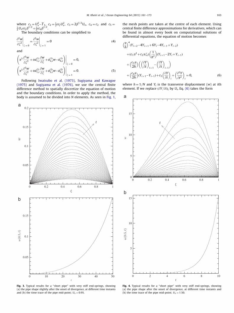
Fig. 3. Typical results for a ‘‘short pipe’’ with very stiff end-springs, showing

(a) the pipe shape slightly after the onset of divergence, at different time instants

and (b) the time trace of the pipe mid-point; Ux ¼ 0:95.

the mesh points are taken at the centre of each element. Usingcentral finite difference approximations for derivatives, which canbe found in almost every book on computational solutions ofdifferential equations, the equation of motion becomes

ah

� �4

ðYiþ2�4Yiþ1þ6Yi�4Yi�1þYi�2Þ

þðc1a2þc2axiÞ1

h2

� �ðYiþ1�2YiþYi�1Þ

þc3a2h

� � @Y

@t

� �iþ1

�@Y

@t

� �i�1

� �

þc4a2h

� �ðYiþ1�Yi�1Þþc5

@Y

@t

� �i

þ@2Y

@t2

� �i

¼ 0, ð6Þ

where h¼ 1=N and Yi is the transverse displacement (w) at ithelement. If we replace ð@Y=@tÞi by Ui, Eq. (6) takes the form

0 0.2 0.4 0.6 0.8 10

5

10

15

0 2 4 6 8 10

5

10

15

Fig. 4. Typical results for a ‘‘short pipe’’ with very stiff end-springs, showing

(a) the pipe shape after the onset of divergence, at different time instants and

(b) the time trace of the pipe mid-point; Ux ¼ 1:50.

M. Kheiri et al. / Ocean Engineering 64 (2013) 161–173164

@U

@t

� �i

¼�c5Ui�c3a2h

� �Uiþ1þ

c3a2h

� �Ui�1�

ah

� �4

Yiþ2

þ�c4a

2h�ðc1a2þc2axiÞ

h2þ4

ah

� �4� �

Yiþ1

þ2ðc1a2þc2axiÞ

h2�6

ah

� �4� �

Yi

þc4a2h

� ��ðc1a2þc2axiÞ

h2þ4

ah

� �4� �

Yi�1

�ah

� �4

Yi�2,@Y

@t

� �i

¼Ui: ð7Þ

0 0.2 0.4 0.6 0.8 1

0

5

10

15

0 2 4 6 8 10

2

4

6

8

10

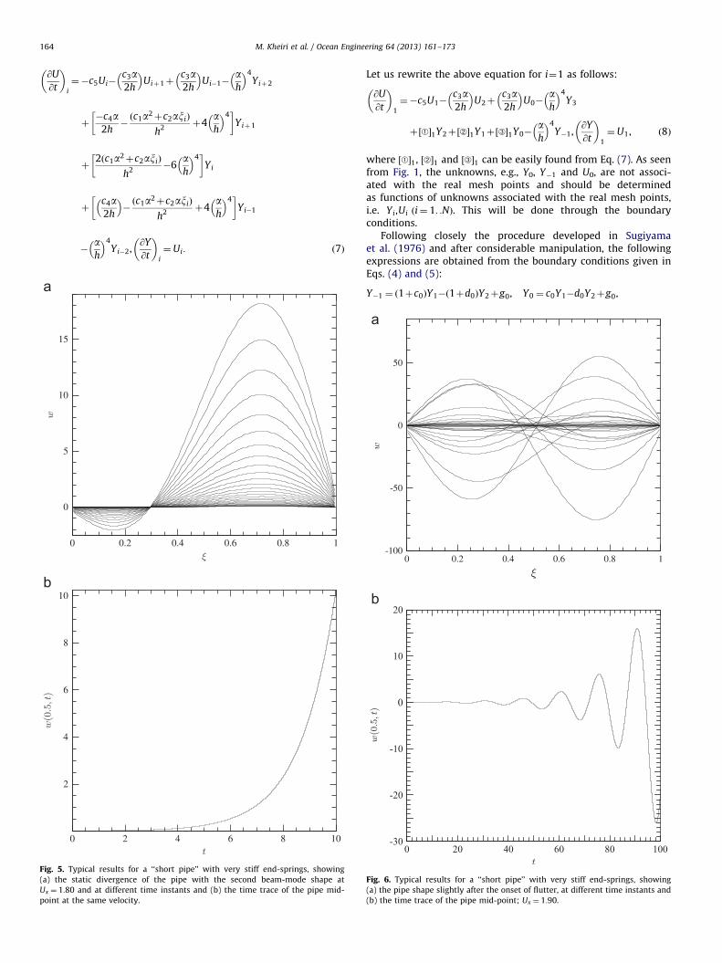
Fig. 5. Typical results for a ‘‘short pipe’’ with very stiff end-springs, showing

(a) the static divergence of the pipe with the second beam-mode shape at

Ux ¼ 1:80 and at different time instants and (b) the time trace of the pipe mid-

point at the same velocity.

Let us rewrite the above equation for i¼1 as follows:

@U

@t

� �1

¼�c5U1�c3a2h

� �U2þ

c3a2h

� �U0�

ah

� �4

Y3

þ½A�1Y2þ½B�1Y1þ½C�1Y0�ah

� �4

Y�1,@Y

@t

� �1

¼U1, ð8Þ

where ½A�1, ½B�1 and ½C�1 can be easily found from Eq. (7). As seenfrom Fig. 1, the unknowns, e.g., Y0, Y�1 and U0, are not associ-ated with the real mesh points and should be determinedas functions of unknowns associated with the real mesh points,i.e. Yi,Ui ði¼ 1: :NÞ. This will be done through the boundaryconditions.

Following closely the procedure developed in Sugiyamaet al. (1976) and after considerable manipulation, the followingexpressions are obtained from the boundary conditions given inEqs. (4) and (5):

Y�1 ¼ ð1þc0ÞY1�ð1þd0ÞY2þg0, Y0 ¼ c0Y1�d0Y2þg0,

0 0.2 0.4 0.6 0.8 1-100

-50

0

50

Fig. 6. Typical results for a ‘‘short pipe’’ with very stiff end-springs, showing

(a) the pipe shape slightly after the onset of flutter, at different time instants and

(b) the time trace of the pipe mid-point; Ux ¼ 1:90.

4E+07

M. Kheiri et al. / Ocean Engineering 64 (2013) 161–173 165

U0 ¼ c0U1�d0U2, ð9Þ

YNþ1 ¼ c1YN�d1YN�1þg1,

YNþ2 ¼ ð1þc1ÞYN�ð1þd1ÞYN�1þg1,

UNþ1 ¼ c1UN�d1UN�1, ð10Þ

where c0 ¼ b0=a0, d0 ¼ 1=a0, g0 ¼ ðd7=2a0N3Þ and a0 ¼ 1�ðd5=4N3

Þ

þðd6=2N2Þ, b0 ¼ 2þðd5=4N3

Þþðd6=2N2Þ in which d5 ¼�ða

ð1Þ3,z=a

3Þ,

0 0.2 0.4 0.6 0.8 1

-4000

-3000

-2000

-1000

0

1000

2000

0 0.2 0.4 0.6 0.8 1-20

-10

0

10

20

30

40

50

60

70

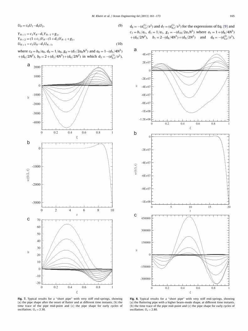
Fig. 7. Typical results for a ‘‘short pipe’’ with very stiff end-springs, showing

(a) the pipe shape after the onset of flutter and at different time instants, (b) the

time trace of the pipe mid-point and (c) the pipe shape for early cycles of

oscillation; Ux ¼ 2:30.

d6 ¼�ðað1Þ1,z=a

2Þ and d7 ¼ ðað1Þ4,z=a

3Þ for the expressions of Eq. (9) and

c1 ¼ b1=a1, d1 ¼ 1=a1, g1 ¼�ðd10=2a1N3Þ where a1 ¼ 1þðd8=4N3

Þ

þðd9=2N2Þ, b1 ¼ 2�ðd8=4N3

Þþðd9=2N2Þ and d8 ¼�ða

ð2Þ3,z=a

3Þ,

0 0.2 0.4 0.6 0.8 1

-1.2E+08

-1E+08

-8E+07

-6E+07

-4E+07

-2E+07

0

2E+07

0 5 10 15 20

-1E+08

-8E+07

-6E+07

-4E+07

-2E+07

0

0 0.2 0.4 0.6 0.8 1

-300000

-150000

0

150000

300000

450000

Fig. 8. Typical results for a ‘‘short pipe’’ with very stiff end-springs, showing

(a) the fluttering pipe with a higher beam-mode shape, at different time instants,

(b) the time trace of the pipe mid-point and (c) the pipe shape for early cycles of

oscillation; Ux ¼ 2:80.

M. Kheiri et al. / Ocean Engineering 64 (2013) 161–173166

d9 ¼�ðað2Þ1,z=a

2Þ and d10 ¼ ðað2Þ4,z=a

3Þ for the expressions of Eq. (10).

The details of how Eqs. (9) and (10) are obtained are given inAppendix A.

After applying the expressions given in Eqs. (9) and (10),Eq. (7) can be completely cast in first-order form,

_X ¼ AXþB, ð11Þ

where X ¼ ½U1 U2 . . .UN Y1 Y2 . . .YN�T and ð_Þ ¼ @ð Þ=@t. Eq. (11) can

be solved numerically via several available mathematicalpackages, such as DIVPAG of IMSL Library and ODE functions ofMATLAB.

2.1.1. Numerical results for short pipes

For validation purposes, several calculations have been per-formed for relatively small values of e, with very large end-springstiffnesses at both upstream and downstream ends and with zerocross-flow, so as to come close to the pinned–pinned systemsstudied before by Paıdoussis (1966, 1973) and others.

0 5 10 15 20-1E+08

-8E+07

-6E+07

-4E+07

-2E+07

0

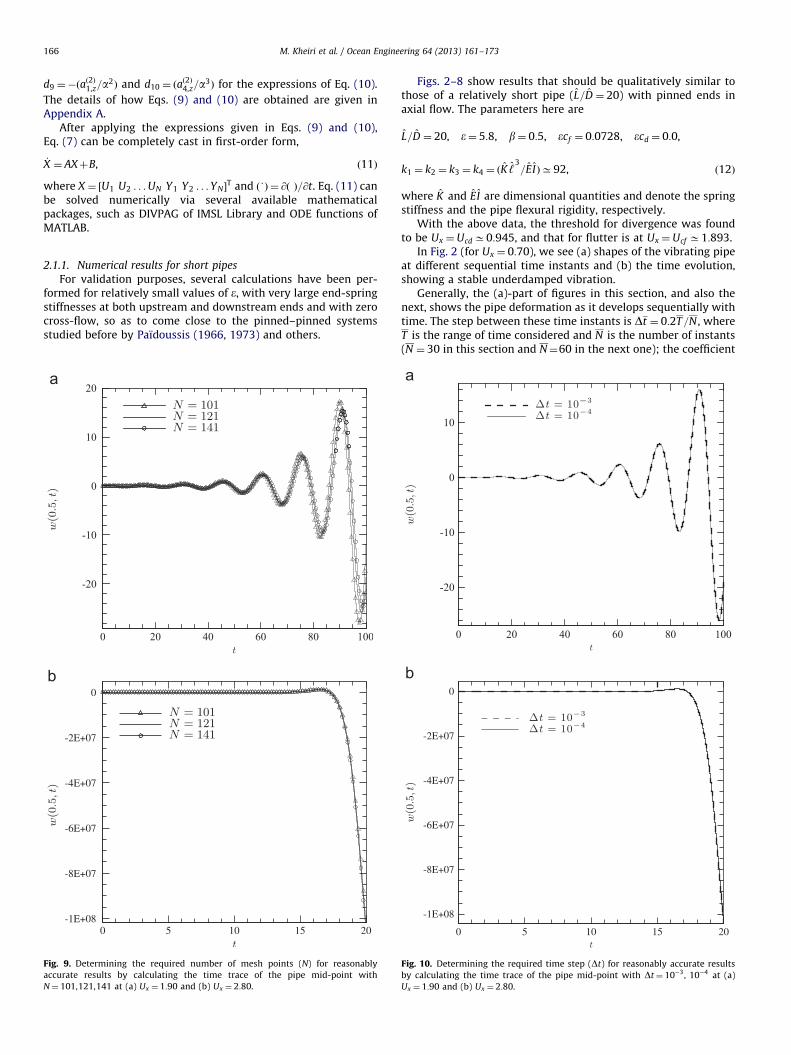
Fig. 9. Determining the required number of mesh points (N) for reasonably

accurate results by calculating the time trace of the pipe mid-point with

N¼ 101,121,141 at (a) Ux ¼ 1:90 and (b) Ux ¼ 2:80.

Figs. 2–8 show results that should be qualitatively similar tothose of a relatively short pipe (L=D ¼ 20) with pinned ends inaxial flow. The parameters here are

L=D ¼ 20, e¼ 5:8, b¼ 0:5, ecf ¼ 0:0728, ecd ¼ 0:0,

k1 ¼ k2 ¼ k3 ¼ k4 ¼ ðK ‘3=EIÞC92, ð12Þ

where K and EI are dimensional quantities and denote the springstiffness and the pipe flexural rigidity, respectively.

With the above data, the threshold for divergence was foundto be Ux ¼UcdC0:945, and that for flutter is at Ux ¼Ucf C1:893.

In Fig. 2 (for Ux ¼ 0:70), we see (a) shapes of the vibrating pipeat different sequential time instants and (b) the time evolution,showing a stable underdamped vibration.

Generally, the (a)-part of figures in this section, and also thenext, shows the pipe deformation as it develops sequentially withtime. The step between these time instants is Dt ¼ 0:2T=N , whereT is the range of time considered and N is the number of instants(N ¼ 30 in this section and N¼60 in the next one); the coefficient

0 5 10 15 20

-1E+08

-8E+07

-6E+07

-4E+07

-2E+07

0

Fig. 10. Determining the required time step (Dt) for reasonably accurate results

by calculating the time trace of the pipe mid-point with Dt¼ 10�3 , 10�4 at (a)

Ux ¼ 1:90 and (b) Ux ¼ 2:80.

M. Kheiri et al. / Ocean Engineering 64 (2013) 161–173 167

0.2 means that the deformed shapes belong to the last 20% of thetime-domain solution.

In Fig. 3, we see the dynamics at Ux ¼ 0:95. In Fig. 3(a), thedeformation is plotted as time is increased, showing clearlythe occurrence of divergence. It is seen that the divergence is inthe form of the first beam-mode shape. The growth of divergenceis also seen clearly in Fig. 3(b), where the mid-point deformationis plotted versus t.

Fig. 4 presents similar results, at Ux ¼ 1:50, showing that thestatic divergence continues to higher flow velocities, with largeramplitudes and asymmetric deformed shape.

In Fig. 5(a) (for Ux ¼ 1:80), we see the transformation of thestatic divergence from one of basically first beam-mode shape (asin Figs. 3(a) and 4(a)) to one of second beam-mode shape. Thistransformation does not occur suddenly at Ux ¼ 1:80; in fact, itstarts at about Ux ¼ 1:50 and develops gradually with increasingflow velocity.

At Ux ¼ 1:90, the pipe becomes dynamically unstable, devel-oping a second beam-mode oscillation, as shown in Fig. 6(a).

0.010.11

0.21

0.31

0.41

0.31

0.41

0.51

0.61

0 0.002 0.004 0.006 0.008 0.01

-0.04

-0.02

0

0.02

0.04

.0.01

0.110.21

0.31 0.410.510.61

0.710.81

0.911.01

1.11

1.11

1.21

1.31

0 0.01 0.02 0.03 0.04 0.05-0.06

-0.04

-0.02

0

0.02

0.04

0.06

0.08

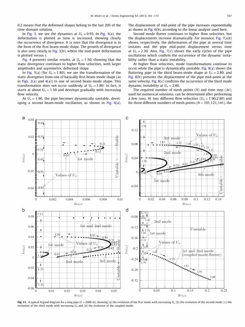
Fig. 11. A typical Argand diagram for a long pipe (L ¼ 2000 m), showing (a) the evolutio

evolution of the third mode with increasing Ux and (d) the evolution of the coupled-m

The displacement of mid-point of the pipe increases exponentiallyas shown in Fig. 6(b), according to the linear analysis used here.

Second mode flutter continues to higher flow velocities, butthe displacements increase dramatically. For instance, Fig. 7(a,b)shows, respectively, the deformation of the pipe at several timeinstants and the pipe mid-point displacement versus timeat Ux ¼ 2:30. Also, Fig. 7(c) shows the early cycles of the pipeoscillations which confirm the occurrence of the dynamic insta-bility rather than a static instability.

At higher flow velocities, mode transformations continue tooccur while the pipe is dynamically unstable. Fig. 8(a) shows thefluttering pipe in the third beam-mode shape at Ux ¼ 2:80, andFig. 8(b) presents the displacement of the pipe mid-point at thesame velocity. Fig. 8(c) confirms the occurrence of the third modedynamic instability at Ux ¼ 2:80.

The required number of mesh points (N) and time step (Dt),used for numerical solutions, can be determined after performinga few runs. At two different flow velocities (Ux ¼ 1:90,2:80) andfor three different numbers of mesh points (N¼ 101,121,141), the

n of the first mode with increasing Ux, (b) the evolution of the second mode, (c) the

ode.

0 0.2 0.4 0.6 0.8 1

0.005

0.01

0.015

M. Kheiri et al. / Ocean Engineering 64 (2013) 161–173168

time trace of the pipe mid-point has been calculated (see Fig. 9).Moreover, at the same flow velocities, the displacement of thepipe mid-point has been obtained versus time with two differenttime steps (Dt¼ 10�3, 10�4) and is plotted in Fig. 10. Thesemainly qualitative comparisons show that the dynamic responsescan be predicted reasonably accurately if N¼121 and Dt¼ 10�3

are used. Some numerical experiments have also been performedto quantitatively study mesh independence. Thus, for the para-meters given in (12) and for several numbers of mesh points(N¼ 101,121,141,161), the onset of instability has been obtainedfor divergence and flutter. It is found that using N¼121 results invalues with less than 1% error.

The results presented above for the short pipe, with para-meters as in Eq. (12), subjected to axial flow can be comparedwith the previous results obtained by Paıdoussis (1973, 1966).It was found previously (Paıdoussis, 1973) that a simply supported(pinned–pinned) pipe, subjected to axial flow, with similar para-meters (b¼ 0:48 rather than 0.50) first loses stability by diver-gence at uC3:14. This is then followed by another divergence atuC6:28, which sensibly coincides with the onset of flutter. Sincedifferent nondimensionalization schemes have been used in this

0 0.2 0.4 0.6 0.8 1

-1.5E-05

-1E-05

-5E-06

0

Fig. 12. Typical results for a ‘‘long pipe’’, showing (a) the shape of the pipe at

different time instants and (b) the time trace of the pipe at x¼ 0:8; Ux ¼ 0:25.

Fig. 13. Typical results for a ‘‘long pipe’’, showing (a) the shape of the pipe slightly

after the onset of divergence and at different time instants and (b) the time trace

of the pipe at x¼ 0:8; Ux ¼ 0:35.

study and in Paıdoussis (1973),1 the critical values found hereneed to be converted; they become ucdC3:25 and ucf C6:50,accordingly, and they are about 3.5% higher than the valuesobtained in Paıdoussis (1973). This difference may be linked tothe fact that, although the end-springs are set to be very stiff inthe present model, they may not perfectly result in ideal pinned–pinned boundary conditions; the difference between the massratios (b¼ 0:5 here and b¼ 0:48 in Paıdoussis, 1973) may alsocause some deviation in the critical value for flutter. [InPaıdoussis (1966), where the viscous forces had been resolvederroneously, a system with b¼ 0:50 loses stability in its firstmode in essentially the same manner as in Paıdoussis (1973) andat the same value of u (ucdC3:14). However, the post-divergencecharacteristics are different, mostly qualitatively (the critical flowvelocity for flutter, ucf, is lower in Paıdoussis (1966) by about 2%)].

1 The nondimensional flow velocity is defined as u¼ ðrA=E IÞ1=2U L in

Paıdoussis (1973), while here it is U ¼ ðrA=E IÞ1=2U ‘ .

M. Kheiri et al. / Ocean Engineering 64 (2013) 161–173 169

2.1.2. Numerical results for long pipes

The numerical results for the dynamics of very long pipesfound in real applications are discussed next. The pipes areconsidered to be 500–3000 m long, and they are made of stainlesssteel. The diameter and thickness of the pipes are chosen based onstandard handbook values found for real applications.

It can easily be shown that, if K 1 ¼ K 2 and K 3 ¼ K 4, B inEq. (11) becomes null, and therefore _X ¼ AX, which is a standardeigenvalue problem. By solving this problem the system beha-viour can be determined accurately.

A standard way of presenting the solution is to plot theevolution of the system eigenfrequencies (o), which are generallycomplex, as an Argand diagram, i.e. in a plane where the abscissaand the ordinate correspond to the real and imaginary part of theeigenfrequencies (ReðoÞ and ImðoÞ), respectively, as a systemparameter varies.

A typical Argand diagram, which displays the evolution of systemnondimensional eigenfrequencies (o) as the nondimensional flow

0 0.2 0.4 0.6 0.8 10

1

2

3

4

5

6

7

0 50 100 150 2000

0.2

0.4

0.6

0.8

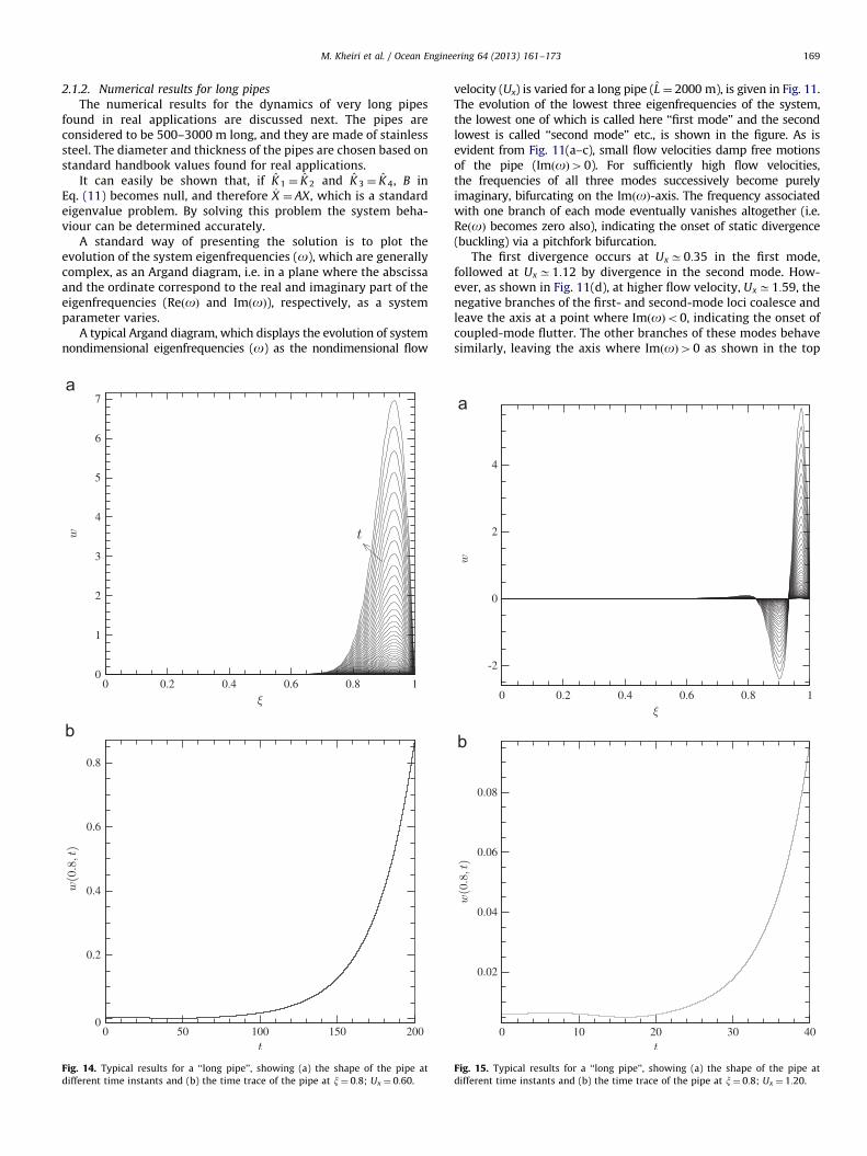
Fig. 14. Typical results for a ‘‘long pipe’’, showing (a) the shape of the pipe at

different time instants and (b) the time trace of the pipe at x¼ 0:8; Ux ¼ 0:60.

velocity (Ux) is varied for a long pipe (L ¼ 2000 m), is given in Fig. 11.The evolution of the lowest three eigenfrequencies of the system,the lowest one of which is called here ‘‘first mode’’ and the secondlowest is called ‘‘second mode’’ etc., is shown in the figure. As isevident from Fig. 11(a–c), small flow velocities damp free motionsof the pipe (ImðoÞ40). For sufficiently high flow velocities,the frequencies of all three modes successively become purelyimaginary, bifurcating on the ImðoÞ-axis. The frequency associatedwith one branch of each mode eventually vanishes altogether (i.e.ReðoÞ becomes zero also), indicating the onset of static divergence(buckling) via a pitchfork bifurcation.

The first divergence occurs at UxC0:35 in the first mode,followed at UxC1:12 by divergence in the second mode. How-ever, as shown in Fig. 11(d), at higher flow velocity, UxC1:59, thenegative branches of the first- and second-mode loci coalesce andleave the axis at a point where ImðoÞo0, indicating the onset ofcoupled-mode flutter. The other branches of these modes behavesimilarly, leaving the axis where ImðoÞ40 as shown in the top

0 0.2 0.4 0.6 0.8 1

-2

0

2

4

0 10 20 30 40

0.02

0.04

0.06

0.08

Fig. 15. Typical results for a ‘‘long pipe’’, showing (a) the shape of the pipe at

different time instants and (b) the time trace of the pipe at x¼ 0:8; Ux ¼ 1:20.

M. Kheiri et al. / Ocean Engineering 64 (2013) 161–173170

part of Fig. 11(b). Finally, at UxC1:99 there is divergence in thethird mode (see Fig. 11(c)).

In order to display the dynamical behaviour of a long pipevisually, the shape of the pipe (with the same parameters as givenabove) is plotted versus time at certain flow velocities(Ux ¼ 0:25,0:35,0:60,1:20 and 1.65) in the (a) part of Figs. 12–16.Also, the time trace of a specific point of the pipe is given for eachof the flow velocities in the (b) part of the figures. This specificpoint is usually x¼ 0:5 for short simply supported pipes, asplotted in Figs. 2(b)– 8(b). However, for long pipes the deflectionsof the mid-pipe (x¼ 0:5) may not be a good choice for properlyillustrating the dynamical behaviour of the system. In fact,a previous study on long cantilevered cylinders subjected to axial

0 0.2 0.4 0.6 0.8 1

-20000

-15000

-10000

-5000

0

5000

10000

0 0.2 0.4 0.6 0.8 1

-5E+17

0

5E+17

1E+18

0 50 100 150 200

-8E+16

-6E+16

-4E+16

-2E+16

0

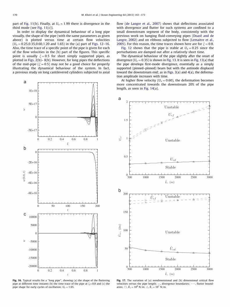
Fig. 16. Typical results for a ‘‘long pipe’’, showing (a) the shape of the fluttering

pipe at different time instants (b) the time trace of the pipe at x¼0.8 and (c) the

pipe shape for early cycles of oscillation; Ux ¼ 1:65.

flow (de Langre et al., 2007) shows that deflections associatedwith divergence and flutter for such systems are confined to asmall downstream segment of the body, consistently with theprevious work on hanging fluid-conveying pipes (Doare and deLangre, 2002) and on ribbons subjected to flow (Lemaitre et al.,2005). For this reason, the time traces shown here are for x¼ 0:8.

Fig. 12 shows that the pipe is stable at Ux ¼ 0:25 since theperturbations are damped out after a relatively short time.

The dynamical behaviour of the pipe slightly after the onset ofdivergence (Ux ¼ 0:35) is shown in Fig. 13. It is seen in Fig. 13(a) thatthe pipe develops first-mode divergence, essentially as a simplysupported (pinned–pinned) beam but with the antinode displacedtoward the downstream end; as in Figs. 3(a) and 4(a), the deforma-tion amplitude increases with time.

At higher flow velocity (Ux ¼ 0:60), the deformation becomesmore concentrated towards the downstream 20% of the pipelength, as seen in Fig. 14(a).

500 1000 1500 2000 2500 30000

0.5

1

1.5

2

500 1000 1500 2000 2500 30000

50

100

150

200

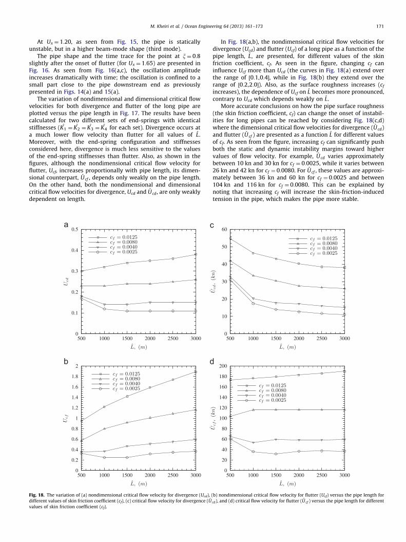
Fig. 17. The variation of (a) nondimensional and (b) dimensional critical flow

velocities versus the pipe length; —, divergence boundaries; - - -, flutter bound-

aries; &, K i ¼ 108 N=m; n, K i ¼ 107 N=m.

M. Kheiri et al. / Ocean Engineering 64 (2013) 161–173 171

At Ux ¼ 1:20, as seen from Fig. 15, the pipe is staticallyunstable, but in a higher beam-mode shape (third mode).

The pipe shape and the time trace for the point at x¼ 0:8slightly after the onset of flutter (for Ux ¼ 1:65) are presented inFig. 16. As seen from Fig. 16(a,c), the oscillation amplitudeincreases dramatically with time; the oscillation is confined to asmall part close to the pipe downstream end as previouslypresented in Figs. 14(a) and 15(a).

The variation of nondimensional and dimensional critical flowvelocities for both divergence and flutter of the long pipe areplotted versus the pipe length in Fig. 17. The results have beencalculated for two different sets of end-springs with identicalstiffnesses (K1 ¼ K2 ¼ K3 ¼ K4 for each set). Divergence occurs ata much lower flow velocity than flutter for all values of L.Moreover, with the end-spring configuration and stiffnessesconsidered here, divergence is much less sensitive to the valuesof the end-spring stiffnesses than flutter. Also, as shown in thefigures, although the nondimensional critical flow velocity forflutter, Ucf, increases proportionally with pipe length, its dimen-sional counterpart, U cf , depends only weakly on the pipe length.On the other hand, both the nondimensional and dimensionalcritical flow velocities for divergence, Ucd and U cd, are only weaklydependent on length.

500 1000 1500 2000 2500 30000

0.1

0.2

0.3

0.4

0.5

500 1000 1500 2000 2500 30000

0.2

0.4

0.6

0.8

1

1.2

1.4

1.6

1.8

2

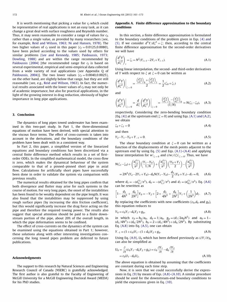
Fig. 18. The variation of (a) nondimensional critical flow velocity for divergence (Ucd),

different values of skin friction coefficient (cf), (c) critical flow velocity for divergence (U

values of skin friction coefficient (cf).

In Fig. 18(a,b), the nondimensional critical flow velocities fordivergence (Ucd) and flutter (Ucf) of a long pipe as a function of thepipe length, L, are presented, for different values of the skinfriction coefficient, cf. As seen in the figure, changing cf caninfluence Ucf more than Ucd (the curves in Fig. 18(a) extend overthe range of ½0:1,0:4�, while in Fig. 18(b) they extend over therange of ½0:2,2:0�). Also, as the surface roughness increases (cf

increases), the dependence of Ucf on L becomes more pronounced,contrary to Ucd which depends weakly on L.

More accurate conclusions on how the pipe surface roughness(the skin friction coefficient, cf) can change the onset of instabil-ities for long pipes can be reached by considering Fig. 18(c,d)where the dimensional critical flow velocities for divergence (U cd)and flutter (U cf ) are presented as a function L for different valuesof cf. As seen from the figure, increasing cf can significantly pushboth the static and dynamic instability margins toward highervalues of flow velocity. For example, U cd varies approximatelybetween 10 kn and 30 kn for cf ¼ 0:0025, while it varies between26 kn and 42 kn for cf ¼ 0:0080. For U cf , these values are approxi-mately between 36 kn and 60 kn for cf ¼ 0:0025 and between104 kn and 116 kn for cf ¼ 0:0080. This can be explained bynoting that increasing cf will increase the skin-friction-inducedtension in the pipe, which makes the pipe more stable.

500 1000 1500 2000 2500 30000

10

20

30

40

50

60

500 1000 1500 2000 2500 30000

20

40

60

80

100

120

140

160

180

200

(b) nondimensional critical flow velocity for flutter (Ucf) versus the pipe length for

cd), and (d) critical flow velocity for flutter (U cf ) versus the pipe length for different

M. Kheiri et al. / Ocean Engineering 64 (2013) 161–173172

It is worth mentioning that picking a value for cf which couldbe representative of real applications is not an easy task, as it canchange a great deal with surface roughness and Reynolds number.Thus, it may seem reasonable to consider a range of values for cf,rather than a single value, as provided by many researchers (see,for example, Reid and Wilson, 1963; Ni and Hansen, 1978). Thetwo higher values of cf used in this paper (cf ¼ 0:0125,0:0080),have been picked according to the values used by others forsimilar problems (Lee and Kennedy, 1985; Paıdoussis, 1973;Dowling, 1988) and are within the range recommended byPaıdoussis (2004) [the recommended range for cf is based onseveral experimental, empirical and semi-empirical data collectedfrom a wide variety of real applications (see Appendix Q ofPaıdoussis, 2004)]. The two lower values (cf ¼ 0:0040,0:0025),on the other hand, are slightly below that range, but they are stillreasonable (see, e.g., Reid and Wilson, 1963). In fact, the numer-ical results associated with the lower values of cf may not only beof academic importance, but also for practical applications, in thelight of the growing interest in drag reduction, obviously of higherimportance in long pipe applications.

3. Conclusion

The dynamics of long pipes towed underwater has been exam-ined in this two-part study. In Part 1, the three-dimensionalequations of motion have been derived, with special attention tothe viscous force terms. The effect of cross-currents is taken intoaccount in the derivations, and the boundary conditions of theproblem have been dealt with in a consistent way.

In Part 2, this paper, a simplified version of the linearizedequations and boundary conditions has been discretized via acentral finite difference method which results in a set of first-order ODEs. In the simplified mathematical model, the cross-flowis zero, which makes the dynamical behaviour of the systemcomparable to that of a pinned–pinned short pipe in axialflow. Calculations for artificially short pipes have successfullybeen done in order to validate the system via comparison withprevious results.

The numerical results obtained for the long pipes confirm thatboth divergence and flutter may arise for such systems in thecourse of motion. For very long pipes, the onset of the instabilitieshas been found to be weakly dependent on the pipe length. It wasalso found that the instabilities may be suppressed by usingrough surface pipes (by increasing the skin friction coefficient),but this would significantly increase the drag force acting on thepipe and therefore the required towing power. The results alsosuggest that special attention should be paid to a finite down-stream portion of the pipe, about 20% of the overall length, inwhich the pipe deformation seems to be confined.

The effect of cross-currents on the dynamics of the system canbe examined using the equations obtained in Part 1; however,these solutions along with other interesting investigations con-cerning the long towed pipes problem are deferred to futurepublications.

Acknowledgments

The support to this research by Natural Sciences and EngineeringResearch Council of Canada (NSERC) is gratefully acknowledged.The first author is also grateful to the Faculty of Engineering ofMcGill University for a McGill Engineering Doctoral Award (MEDA)for his PhD studies.

Appendix A. Finite difference approximation to the boundaryconditions

In this section, a finite difference approximation is formulatedto the boundary conditions of the problem given in Eqs. (4) and(5). If we consider d2Y=dx2

¼ z; then, according to the centralfinite difference approximation for the second-order derivativeswe will have

d2Y

dx2

!i

¼ zi ¼N2ðYiþ1�2YiþYi�1Þ: ðA:1Þ

Using linear interpolation, the second- and third-order derivativesof Y with respect to x at x¼ 0 can be written as

d2Y

dx2

!�����x ¼ 0

¼

d2Ydx2

� �0þ d2Y

dx2

� �1

2¼

1

2ðz0þz1Þ ðA:2Þ

and

d3Y

dx3

!�����x ¼ 0

¼d

dxd2Y

dx2

!�����x ¼ 0

¼

d2Ydx2

� �1� d2Y

dx2

� �0

ð1=NÞ¼Nðz1�z0Þ, ðA:3Þ

respectively. Considering the zero-bending boundary condition(Eq. (4)) at the upstream end (x¼ 0) and using Eqs. (A.1) and (A.2),we obtain

z0þz1 ¼ 0 ðA:4Þ

and then

Y2�Y1�Y0þY�1 ¼ 0: ðA:5Þ

The shear boundary condition at x¼ 0 can be written as afunction of the displacements of the mesh points adjacent to theupstream end by using Eq. (5) and Eqs. (A.1)–(A.4) and applyinglinear interpolation for w9x ¼ 0 and ð@w=@xÞ9x ¼ 0. Thus, we have

Nðz1�z0Þþað1Þ1,z

a2

!Y1�Y0

1=N

� �þ

að1Þ3,z

a3

!Y0þY1

2

� ��

að1Þ4,z

a3

!

¼ 2N3ðY2�2Y1þY0Þ�d6NðY1�Y0Þ�

d5

2ðY0þY1Þ�d7 ¼ 0, ðA:6Þ

where d5 ¼�ðað1Þ3,z=a

3Þ, d6 ¼�ðað1Þ1,z=a

2Þ and d7 ¼ ðað1Þ4,z=a

3Þ. Eq. (A.6)can be rewritten as

1�d5

4N3þ

d6

2N2

� �Y0 ¼�Y2þ 2þ

d5

4N3þ

d6

2N2

� �Y1þ

1

2N3

� �d7: ðA:7Þ

By replacing the coefficients with new coefficients (c0,d0 and g0),this equation reduces to

Y0 ¼ c0Y1�d0Y2þg0, ðA:8Þ

in which c0 ¼ b0=a0, d0 ¼ 1=a0, g0 ¼ ðd7=2a0N3Þ and a0 ¼ 1�

ðd5=4N3Þþðd6=2N2

Þ, b0 ¼ 2þðd5=4N3Þþðd6=2N2

Þ. By substitutingEq. (A.8) into Eq. (A.5), one can obtain

Y�1 ¼ ð1þc0ÞY1�ð1þd0ÞY2þg0: ðA:9Þ

Using Eq. (A.9), U0 which has been defined previously as ð@Y=@tÞ0can also be simplified as

U0 ¼@

@tðc0Y1�d0Y2þg0Þ ¼ c0

@Y1

@t�d0

@Y2

@t

¼ c0U1�d0U2: ðA:10Þ

The above equation is obtained by assuming that the coefficientsare constant during each time step.

Now, it is seen that we could successfully derive the expres-sions in Eq. (9) by means of Eqs. (A.8)–(A.10). A similar procedureshould be used for the downstream-end boundary conditions toyield the expressions given in Eq. (10).

M. Kheiri et al. / Ocean Engineering 64 (2013) 161–173 173

References

de Langre, E., Paıdoussis, M.P., Doare, O., Modarres-Sadeghi, Y., 2007. Flutter oflong flexible cylinders in axial flow. J. Fluid Mech. 571, 371–389.

Doare, O., de Langre, E., 2002. The flow-induced instability of long hanging pipes.Eur. J. Mech. A—Solid 21, 857–867.

Dowling, A.P., 1988. The dynamics of towed flexible cylinders. Part 1: neutrallybuoyant elements. J. Fluid Mech. 187, 507–532.

Iwatsubo, T., Saigo, M., Sugiyama, Y., 1973. Parametric instability of clamped–clamped and clamped–simply supported columns under periodic axial load.J. Sound Vib. 30, 65–77.

Lee, D., Kennedy, R.M., 1985. A numerical treatment of a mixed type dynamicmotion equation arising from a towed acoustic antenna in the ocean. Comput.Math. Appl. 11, 807–816.

Lee, T.S., 1981. Stability analysis of the ortloff-ives equation. J. Fluid Mech. 110,293–295.

Lemaitre, C., Hemon, P., de Langre, E., 2005. Instability of a long ribbon hanging inaxial air flow. J. Fluid Struct. 20, 913–925.

Ni, C.C., Hansen, R.J., 1978. An experimental study of the flow-induced motions ofa flexible cylinder in axial flow. ASME J. Fluid. Eng. 100, 389–394.

Ortloff, C.R., Ives, J., 1969. On the dynamic motion of a thin flexible cylinder in aviscous stream. J. Fluid Mech. 38, 713–720.

Paıdoussis, M.P., 1966. Dynamics of flexible slender cylinders in axial flow. Part 1.Theory. J. Fluid Mech. 26, 717–736.

Paıdoussis, M.P., 1968. Stability of towed, totally submerged flexible cylinders. J.Fluid Mech. 34, 273–297.

Paıdoussis, M.P., 1973. Dynamics of cylindrical structures subjected to axial flow. J.Sound Vib. 29, 365–385.

Paıdoussis, M.P., 2004. Fluid–Structure Interactions: Slender Structures and AxialFlow, vol. 2. Elsevier Academic Press, Oxford.

Pao, H.P., 1970. Dynamical stability of a towed thin flexible cylinder. J. Hydronaut.4, 144–150.

Reid, R., Wilson, B., 1963. Boundary flow along a circular cylinder. ASCE J. Hydraul.Div. 89 (HY3), 21–40.

Sudarsan, K., Bhattacharyya, S.K., Vendhan, C.P., 1997. An experimental study ofhydroelastic instability of flexible towed underwater cylindrical structures.In: Proceedings 16th OMAE Conference, Yokohama, Japan, pp. 73–80.

Sugiyama, Y., Kashima, K., Kawagoe, H., 1976. On an unduly simplified model inthe non-conservative problems of elastic stability. J. Sound Vib. 45, 237–247.

Sugiyama, Y., Kawagoe, H., 1975. Vibration and stability of elastic columns underthe combined action of uniformly distributed vertical and tangential forces.J. Sound Vib. 38, 341–355.

Triantafyllou, G.S., Chryssostomidis, C., 1985. Stability of a string in axial flow.ASME J. Energy Resour. Technol. 107, 421–425.