1

1

2

3

4

5

6

7

8

9

Three-Dimensional Flow Visualization and Vorticity Dynamics in 10

Revolving Wings 11

12

13

Authors: Bo Cheng1, Sanjay P. Sane

2, Giovanni Barbera

1, Daniel R. Troolin

3, Tyson Strand

3 14

and Xinyan Deng1* 15

1School of Mechanical Engineering, Purdue University, West Lafayette, IN 47907, USA 16

2National Centre for Biological Sciences, Tata Institute of Fundamental Research, GKVK 17

Campus, Bellary Road, Bangalore 560 065, India 18

3Fluid Mechanics Division, TSI Incorporated, Saint Paul, MN 55126, USA 19

*Author for correspondence (xdeng@purdue.edu; phone# 765-494-1513; fax# 765-494-0539) 20

21

22

23

2

Abstract 24

We investigated the three-dimensional vorticity dynamics of the flows generated by revolving 25

wings using a volumetric 3-component velocimetry (V3V) system. The three-dimensional 26

velocity and vorticity fields were represented with respect to the base axes of rotating 27

Cartesian reference frames, and the second invariant of the velocity gradient was evaluated 28

and used as a criterion to identify two core vortex structures. The first structure was a 29

composite of leading, trailing and tip-edge vortices attached to the wing edges, whereas the 30

second structure was a strong tip vortex tilted from leading-edge vortices and shed into the 31

wake together with the vorticity generated at the tip edge. Using the fundamental vorticity 32

equation, we evaluated the convection, stretching and tilting of vorticity in the rotating wing 33

frame to understand the generation and evolution of vorticity. Based on these data, we 34

propose that the vorticity generated at the leading edge is carried away by strong tangential 35

flow into the wake and travels downwards with the induced downwash. The convection by 36

spanwise flow is comparatively negligible. The three-dimensional flow in the wake also 37

exhibits considerable vortex tilting and stretching. Together these data underscore the 38

complex and interconnected vortical structures and dynamics generated by revolving wings. 39

40

1 Introduction 41

The flapping wings of insects operate at high angles of attack and generate strong 42

unsteady aerodynamic and three-dimensional phenomena (Maxworthy 1981; Willmott et al. 43

1997; Sane 2003; Kim and Gharib 2010). Unlike conventional fixed wings which stall at high 44

angles of attack due to instability of the vortex structures on the wing, insect wings in 45

flapping or revolving motions are able to generate high forces and stable flows in a sustained 46

manner throughout the duration of their motion. Recently, several studies have focused on the 47

mechanisms that underlie the high force generation and stable vortices on flapping/revolving 48

wings (Willmott et al. 1997; Birch and Dickinson 2001; Lentink and Dickinson 2009b). 49

3

Together these studies show that the stable attachment of a prominent leading-edge 50

vortex (LEV) significantly enhances the lift production as compared to conventional 51

translating wings (Ellington et al. 1996; VandenBerg and Ellington 1997; Usherwood and 52

Ellington 2002; Birch et al. 2004). However, the mechanisms underlying the stability of the 53

LEV have been the subject of some debate prompting researchers to use diverse experimental 54

and theoretical approaches to address this question (e.g., Ellington et al. 1996, Birch and 55

Dickinson 2001, Minotti, 2005, Shyy and Liu 2007). Using smoke flow visualization, 56

Ellington and coworkers (Ellington et al. 1996) demonstrated the presence of spanwise flow 57

within the core of a spiral LEV generated by a flapping wing at Re ~ 3000, similar to that 58

proposed by Maxworthy (1981). They proposed that, similar to the axial flow in the vortex 59

core of Delta wings, the spanwise transport of momentum out of the LEV was critical in 60

keeping the LEV small but stable in flapping wings. Numerical investigations of this flow by 61

Liu and Kawachi (1998) and Lan and Sun (2001) further detailed these phenomena. On the 62

analytical front, Minotti (2005) used inviscid potential theory to derive a theoretical 63

framework that demonstrated a balance between the vorticity generated by the leading edge 64

and that transported by spanwise flow. To test the hypothesis that spanwise transport of 65

vorticity mediated by an axial flow keeps it small and stable, Birch and coworkers (Birch and 66

Dickinson 2001; Birch et al. 2004) placed orthogonal plates along the wing span to limit the 67

span wise flow at Re ~ 200. They found that even under these conditions, the wing continued 68

to generate a stable LEV. To explain this discrepancy, Birch and Dickinson proposed that 69

strong downward flow induced by the flapping wings limits the growth of the LEV (Birch 70

and Dickinson 2001). These results were in agreement with computational fluid dynamics-71

based simulations of flows under similar conditions (Shyy and Liu 2007). 72

To experimentally test the hypothesis that spanwise flow contributes to stabilization 73

of the leading edge vortex, Beem et.al. (2012) used swept and translating, rather than 74

revolving, wings to generate spanwise flows but did not observe significant differences in the 75

time required for break-off and downstream convection of the vortex as compared to wings of 76

lower sweep angles which generate less spanwise flow. Specifically, for cases of low sweep 77

4

angles, they observed the tip vortex and the LEV as being unconnected structures with a 78

pronounced gap region. Reminiscent of the Birch and Dickinson (2001) study, the flow 79

induced by the tip vortex caused a pronounced downwash that prevented flow separation near 80

the tip. For large sweep angles however, the LEV and tip vortices were more connected and 81

inter-dependent. However, they did notice significant differences in the flow topologies of the 82

LEV and tip vortices. These results indicated that in the swept wing case, spanwise flow may 83

not have much influence on the LEV stabilization and attachment. To what extent do these 84

observations apply to flapping wings? Recently, using dynamically-scaled robotic wings, 85

Lentink and Dickinson (2009 a,b) showed that LEV stability is determined by their Rossby 86

numbers (a ratio of inertial force to rotational accelerations, Lentink and Dickinson, 2009b), 87

rather than Reynolds numbers (a ratio of inertial to viscous forces) which only affect the LEV 88

integrity (Fig. 5 in Lentink and Dickinson 2009b). Using 3D flow visualization, Kim and 89

Gharib (2010) showed that spanwise flow is widely distributed in the wake, and suggested 90

that its generation may be attributed to the vorticity tilted from the LEV. 91

It is evident from the above-described research that force and flow generation by 92

flapping wings is distinctly three-dimensional in nature, and thus traditional DPIV which can 93

only image a plane at a time is limited in its ability to rigorously quantify such flows. 94

Developments in the area of three-dimensional particle tracking (e.g. Troolin and Longmire 95

2009; Pereira et al. 2000; Kim and Gharib 2010; Flammang et al. 2011) provide the means to 96

address the above questions relating to flows around flapping wings. Here, we used a 97

technique called volumetric 3-component velocimetry (V3V) to quantify the three-98

dimensional flows around wings revolving at high angles of attack. From the velocity and 99

vorticity fields, we identified the vortex structure from the second invariant of the velocity 100

gradient. By calculating different terms of the vorticity equation, we also quantified the 101

components due to vortex tilting/stretching and convection and thus account for the various 102

terms underlying the balance of leading-edge vorticity. 103

104

5

2 Material and methods 105

2.1 Experimental setup and procedure 106

All experiments reported here were conducted with a dynamically scaled mechanical 107

wing, which was inspired by nature to reproduce the flow and study the aerodynamics in 108

natural fliers (similar setups are described in Sane, 2001, DiLeo 2007). The wing, which was 109

capable of two-degrees-of-freedom rotations about vertical and wing longitudinal axes, was 110

used to produce the revolving motion at a constant angular speed (Ω = 55 degs s-1

). The angle 111

of attack (AOA) was fixed at 45°. Both degrees of freedom were driven by DC motors 112

(Maxon Motor AG, Sachseln, Switzerland). The motion control system used here has been 113

previously detailed in Zhao et al. (2009). The constant angular velocity with fixed angle of 114

attack (AOA) meant that time-dependent effects due to wing acceleration such as added mass 115

could be ignored as they were negligible (Dickinson et al. 1999; Sane and Dickinson 2002). 116

The wing and the gearbox were immersed in the center of a tank (61 × 61 × 305 cm 117

width × height × length) filled with mineral oil (kinematic viscosity 8 cSt at 20ºC, density 118

850 kg m3). A rectangular wing platform was used with a length of 8cm (from wing tip to 119

center of rotation) and aspect ratio of 7 (two times wing length/mean chord length). The wing 120

was made from a transparent polymer sheet with uniform thickness of 0.53 mm, which 121

remained rigid during the experiments. The wing was located approximately 3 wing lengths 122

away from the wall of the tank and therefore any wall effects were negligible according to 123

Sane (2011). 124

The Reynolds number in this study (rectangular wing) was 220 using: 125

126

𝑅𝑒 = 4π𝑅2

𝜐(𝐴𝑅)𝑇 (1) 127

128

where the characteristic velocity is the wing tip velocity (2π

𝑇𝑅) and the characteristic length is 129

the wing mean chord length (𝑐 =2𝑅

𝐴𝑅), 𝑅 is the wing length, 𝐴𝑅 is wing aspect ratio, 𝑇 is 130

6

period of one full revolution (6.5 s), and 𝜐 is the kinematic viscosity of the fluid. 131

2.2 Volumetric 3-component velocimetry process 132

We used a flow measurement technique, known as volumetric 3-component 133

velocimetry (V3V; TSI Inc., Shoreview, MN, USA), first described by Periera et al. (2000), 134

to investigate the three-dimensional flow structure around revolving wings. A similar system 135

has been used in other studies (e.g., Flammang et al. 2011). A schematic of the experimental 136

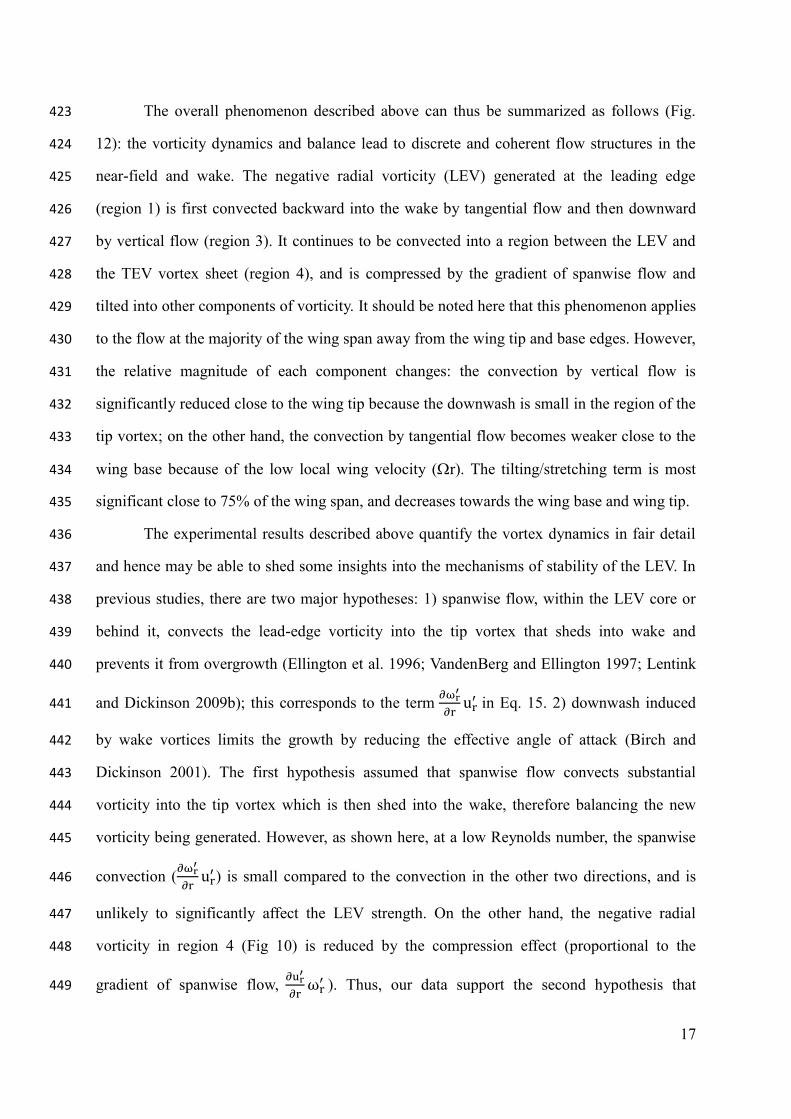
setup can be seen in Fig. 1. We used air bubbles pumped out of a porous ceramic filter as 137

seeding particles (Similar methods were used Birch and Dickinson 2001, and Zhao et al., 138

2011). Experiments were conducted after large bubbles rose to the surface leaving behind 139

only small bubbles with an average size of 20-50 microns. Using Stokes law, this corresponds 140

to a rise velocity of air bubbles in mineral oil of less than 0.17 mm/s (for more description, 141

refer to Zhao et al., 2011). Pairs of sequential images were taken simultaneously by three 4 142

megapixel digital cameras synchronized with an Nd:YAG pulse laser illuminating the air 143

bubbles inside the measurement volume. 144

The fixed coordinate frame (, , ) is attached to the measurement volume defined 145

by the V3V system (Fig. 2a, b). The measurement volume, formed by the intersection of the 146

field of view of the three cameras, was 14 × 14 × 10 cm3 along the , and directions. 147

This volume was sufficient to allow the entire wing to remain within the camera view over a 148

100° rotation. The axis of rotation was positioned at 2cm distance from the back plane of the 149

measurement volume (Fig. 2b) to ensure that there were no laser reflections from the shaft 150

and gearbox. A total of 10 frames, phase-locked to the wing angular position (θ), were 151

captured, allowing consistent captures of a sequence of 10 frames equally spaced at constant 152

Δθ=10°, for a total span of 100°. In this study, we focus only on the steady flow structures of 153

the revolving wing. Hence, in each experiment the image capturing was triggered after one 154

full revolution of the wing to reduce the transient phenomena due to the wing accelerating 155

from rest (Fig. 3). The influence of the vorticity wake from the 1st revolution is considered 156

negligible on the flow in the 2nd

revolution. The 10 frames showed identical flow structure 157

7

with minimal variations, by which we could conservatively assume the flow to have settled 158

into a stable mode. However, the wake generated by the wing was not fully within the 159

volume for some early frames; therefore, to better demonstrate the wake in the center of the 160

volume, results from the 8th

frame are shown. 161

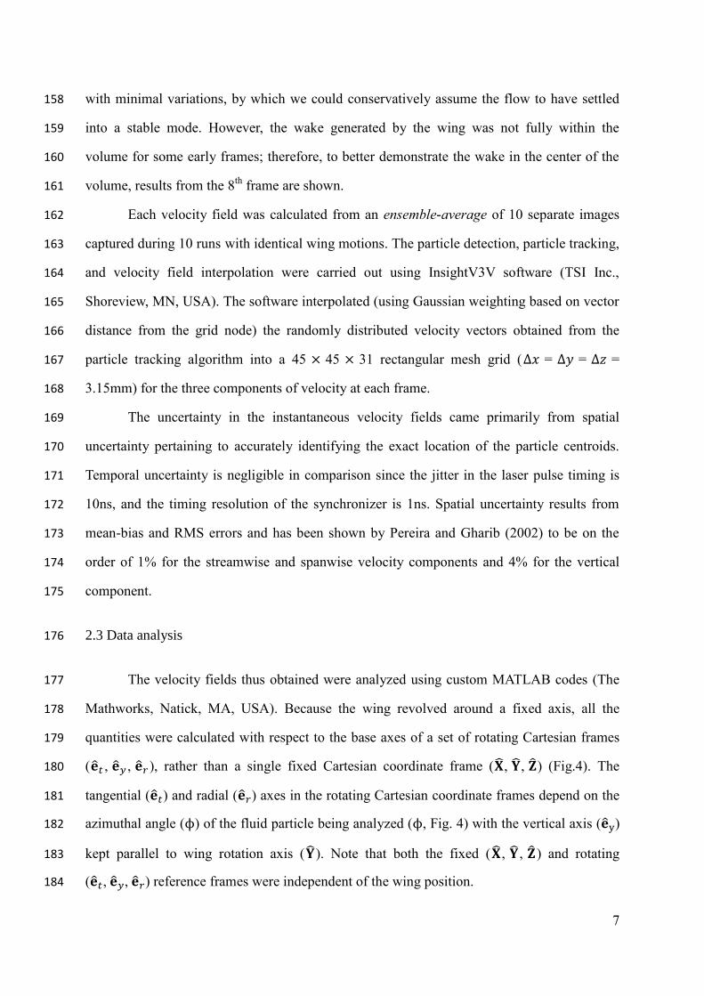
Each velocity field was calculated from an ensemble-average of 10 separate images 162

captured during 10 runs with identical wing motions. The particle detection, particle tracking, 163

and velocity field interpolation were carried out using InsightV3V software (TSI Inc., 164

Shoreview, MN, USA). The software interpolated (using Gaussian weighting based on vector 165

distance from the grid node) the randomly distributed velocity vectors obtained from the 166

particle tracking algorithm into a 45 × 45 × 31 rectangular mesh grid (Δ𝑥 = Δ𝑦 = Δ𝑧 = 167

3.15mm) for the three components of velocity at each frame. 168

The uncertainty in the instantaneous velocity fields came primarily from spatial 169

uncertainty pertaining to accurately identifying the exact location of the particle centroids. 170

Temporal uncertainty is negligible in comparison since the jitter in the laser pulse timing is 171

10ns, and the timing resolution of the synchronizer is 1ns. Spatial uncertainty results from 172

mean-bias and RMS errors and has been shown by Pereira and Gharib (2002) to be on the 173

order of 1% for the streamwise and spanwise velocity components and 4% for the vertical 174

component. 175

2.3 Data analysis 176

The velocity fields thus obtained were analyzed using custom MATLAB codes (The 177

Mathworks, Natick, MA, USA). Because the wing revolved around a fixed axis, all the 178

quantities were calculated with respect to the base axes of a set of rotating Cartesian frames 179

(𝑡 , 𝑦 , 𝑟 ), rather than a single fixed Cartesian coordinate frame (, , ) (Fig.4). The 180

tangential (𝑡) and radial (𝑟) axes in the rotating Cartesian coordinate frames depend on the 181

azimuthal angle (ϕ) of the fluid particle being analyzed (ϕ, Fig. 4) with the vertical axis (y) 182

kept parallel to wing rotation axis (). Note that both the fixed ( , , ) and rotating 183

(𝑡, 𝑦, 𝑟) reference frames were independent of the wing position. 184

8

In the fixed Cartesian reference system, the radial vorticity generated by the wing at a 185

given wing position may get confounded with the tangential vorticity at another wing 186

position. This can be avoided by converting the coordinate system to a rotating Cartesian 187

coordinate frame. The original Cartesian mesh grid and velocity field output from V3V 188

Insight software were converted into base vectors in the rotating Cartesian coordinate frames 189

using the rotation matrix, J(ϕ), such that the velocity components in rotating Cartesian l (ut, 190

uy, ur) and fixed Cartesian frame (ux, uy, uz) are related by: 191

192

𝐮(t, y, r) = (

utuyur) = J𝐮(x, y, z) = J (

uxuyuz) = (

sin(ϕ)ux − cos (ϕ)uzuy

cos (ϕ)ux + sin (ϕ)uz

). (2) 193

194

The same relation also applies to other quantities (e.g., vorticity, vortex tilting and stretching). 195

We calculated the velocity/vorticity gradient tensor with respect to the base vectors in 196

the rotating Cartesian frame. Using chain rule, the gradient tensor in rotating and fixed 197

Cartesian frames are related by 198

199

∇(t,y,r)𝐮(t, y, r) = J∇(t,y,r)𝐮(x, y, z) = J∇(x,y,z)𝐮(x, y, z)JT (3) 200

201

where∇(t,y,r) and ∇(x,y,z) represent the gradient operation in rotating and fixed Cartesian 202

frames, respectively. ∇(t,y,r)𝐮(t, y, r) is the velocity gradient tensor in rotating Cartesian 203

frame, which is (we neglect the subscript in the rest of paper for convenience): 204

205

∇𝐮(t, y, r) =

(

∂ut

∂t

∂ut

∂y

∂ut

∂r

∂uy

∂t

∂uy

∂y

∂uy

∂r

∂ur

∂t

∂ur

∂y

∂ur

∂r )

(4) 206

207

The above relation also applies to the vorticity gradient ∇𝛚 . The wing orientation was 208

determined by tracking four vertices of the wing platform and estimating their spatial 209

9

locations using the calibration process developed for the particle identification. 210

The velocity field, vorticity distribution and vortex structure of the flow were 211

presented by plotting the isosurface for each component of the corresponding quantity 212

separately. Vorticity magnitude isosurfaces were plotted with three different colors (RGB: 213

red, green and blue) indicating the magnitude of positive (red) and negative (blue) 214

components of radial vorticity and negative (green) component of tangential vorticity. Thus, 215

this technique offers clear visualization of both vorticity magnitude and direction within a 216

single isosurface plot. All of the other components (e.g., vertical vorticity) were represented 217

by black coloring. 218

The vortex core structure was evaluated by calculating the second invariant of the 219

velocity gradient, or Q value, calculated using (Jeong and Hussain 1995): 220

221

𝑄 = −1

2(𝜆1 + 𝜆2 + 𝜆3) (5) 222

223

where 𝜆1 , 𝜆2 and 𝜆3 are the eigenvalues of 𝑆2 and Ω2 , where 𝑆 and Ω are the symmetric 224

(1

2(∇𝐮 + ∇𝐮𝑇)) and antisymmetric (

1

2(∇𝐮 − ∇𝐮𝑇)) part of velocity gradient tensor ∇𝐮. 225

Results were non-dimensionalized using the following characteristic values: velocity 226

by wing tip velocity (𝛀R), vorticity by wing rotation vorticity (2𝛀) and time by half period of 227

one wing revolution (π/ 𝛀). All dimensionless quantities are denoted by superscript +. 228

229

2.4 Vorticity equation in rotating frame 230

The standard Navier-Stokes equation for an incompressible fluid may be given by the 231

following pair of equations: 232

233

D𝐮

D𝜏= −∇𝑝 + υ∇2𝐮 (6) 234

∇ ∙ 𝐮 = 0, (7) 235

10

236

where 𝐮 velocity vector, 𝜏 is time, 𝑝 is pressure, υ is kinematic viscosity. The vorticity 237

equation can be derived by taking a curl of (6), which eliminates the pressure term to give, 238

239

∂𝛚

∂𝜏= ∇ × (𝐮 × 𝛚) + υ∇2𝛚, (8) 240

241

which upon expansion gives, 242

243

∂𝛚

∂𝜏= (𝛚 ∙ ∇)𝐮 − (𝐮 ∙ ∇)𝛚 + (∇ ∙ 𝛚)𝐮 − (∇ ∙ 𝐮)𝛚 + υ∇2𝛚 (9) 244

245

In this equation, ∇ ∙ 𝐮 = 𝟎 due to the incompressibility condition and ∇ ∙ 𝛚 = 0 because it is 246

a divergence of a curl of velocity. Rearranging the remaining terms, we get 247

248

D𝛚

D𝜏=∂𝛚

∂𝜏+ (𝐮 ∙ ∇)𝛚 = (𝛚 ∙ ∇)𝐮 + υ∇2𝛚 (10) 249

250

In a rotational Cartesian frame, 251

252

𝛚 = 𝛚′ + 2𝛀 253

𝐮 = 𝐮′ + 𝛀 × 𝐫 254

D𝛚

D𝜏=D𝛚′

D𝜏+ 𝛀 ×𝛚 (11) 255

∇2𝛚 = ∇2𝛚′ 256

∇= ∇′ 257

258

where the superscript ' denotes the relative quantities observed in the rotating frame, 𝐫, is the 259

radial vector with the length from the fluid element to the axis of rotation. Note that D𝛚

D𝜏 and 260

D𝛚′

D𝜏 are the absolute and relative rate of change of vorticity (𝛚) observed in fixed and rotating 261

11

frames, respectively. Also, it can be shown that 𝛀 ×𝛚 is equal to (𝛚 ∙ ∇)(𝛀 × 𝐫). Thus, the 262

vorticity equation in the rotating frame may be written as 263

264

D𝛚′

D𝜏=∂𝛚′

∂𝜏+ (𝐮′ ∙ ∇)𝛚′ = [(𝛚′ + 2𝛀) ∙ ∇]𝐮′ + υ∇2𝛚′, (12) 265

266

where the rate of vorticity change in the rotational frame ( ′ =∂𝛚′

∂𝜏) is equal to the 267

summation of vorticity convection (−(𝐮′ ∙ ∇)𝛚′), vortex tilting and stretching ((𝛚 ∙ ∇)𝐮′) and 268

vorticity diffusion (υ∇2𝛚′). We then separated tilting and stretching components by 269

270

(𝛚 ∙ ∇)𝐮′ = [(𝛚 ∙ ∇)𝐮′]⊥ + [(𝛚 ∙ ∇)𝐮′]∥, (13) 271

272

where [(𝛚 ∙ ∇)𝐮]⊥ is the tilting component and [(𝛚 ∙ ∇)𝐮]∥ is the stretching component, and 273

subscript ⊥ and ∥ denote the projections perpendicular and parallel to the direction of 274

vorticity. Note that, (𝛚 ∙ ∇)𝐮′ includes the vortex tilting and stretching due to wing rotation 275

2𝛀 and relative vorticity 𝛚′. 276

Next, we looked specifically at the radial component, which describes the leading-277

edge (and trailing-edge) vortices generated by the revolving motion. 278

279

ωr′ = (𝛚 ∙ ∇)ur

′ − (𝐮′ ∙ ∇)ωr′ + υ∇2ωr

′ , (14) 280

281

where ur′ = ur and ωr

′ = ωr. The convection term can be expanded as 282

283

(𝐮′ ∙ ∇)ωr′ =

∂ωr′

∂tut′ +

∂ωr′

∂yuy′ +

∂ωr′

∂rur′ , (15) 284

285

where ut′ = ut − 2Ωr and uy

′ = uy. Note that ∂ωr

′

∂tut′ and

∂ωr′

∂yuy′ describe the vorticity transport 286

by tangential and vertical flow; ∂ωr

′

∂rur′ describes the transport by spanwise flow, which was 287

acknowledged in the previous studies as the key mechanism to keep the leading-edge vortex 288

12

stable (e.g., Ellington et al. 1996). Lastly, the tilting and stretching term can be expanded as 289

290

(𝛚 ∙ ∇)ur′ =

∂ur′

∂tωt′ +

∂ur′

∂yωy′ +

∂ur′

∂rωr′ (16) 291

292

where ωt′ = ωt and ωy

′ = ωy − 2Ω. Note that ∂ur′

∂tωt′ and

∂ur′

∂yωy′ describe the vortex tilting 293

from tangential and vertical components; and ∂ur′

∂rωr′ describes the radial vortex stretching. 294

Based on the measured velocity field, all the terms in the vorticity equation described 295

above could be evaluated. We used MATLAB for all the analysis. Derivatives of the velocity 296

and vorticity were calculated using central differencing. No smooth rendering was applied to 297

calculate velocity, vorticity and vortex tilting and stretching terms during post-processing. 298

However, we did smooth the convection terms, which was subject to greater noise due to the 299

vorticity gradient, which was magnified by ambient velocity (2Ωr) factor in the tangential 300

direction (Eq. 15). Specifically, the convection terms at a meshgrid were smoothed out by 301

(weighted) averaging it with the six nearest neighboring points, and the process was iterated 302

five times. 303

304

3 Results and Discussions 305

3.1 Velocity and vorticity fields 306

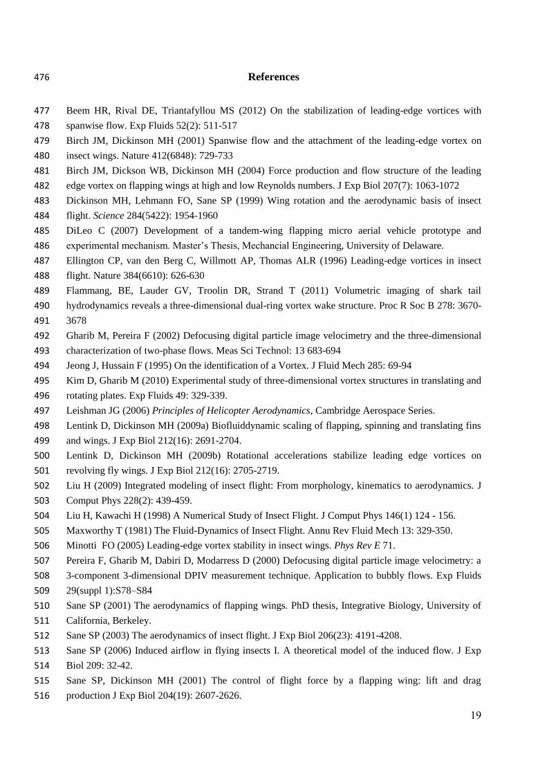
The three-dimensional velocity and vorticity data is shown in Figs. 5 through 7. 307

Figure 5 shows the spatial locations of the 2D slices represented in Figs. 6 and 7, in the 308

context of the measurement volume. In the velocity isosurface plots (Fig. 6a-c), we represent 309

radial components (Fig. 6a) with red (base to tip) and blue (tip to base), the tangential 310

components (Fig. 6b) with green (direction of wing motion) and orange (opposite direction of 311

wing motion), and vertical components (Fig. 6c) with purple (upward) and yellow 312

(downward) colors. 313

13

Several interesting features are identified. First, the spanwise components of the flow 314

are distributed both along the wing tip and downstream to the wake (Fig. 6a, d). The 315

tangential flow in the direction of wing motion (Fig. 6b) is greater than other two components 316

of the flow, and reaches maximum at approximately 80% of the wing span (Fig. 7g). A small 317

upwash (purple) is also found along the leading edge and tip corner (Fig. 6c). Second, there is 318

negligible spanwise flow at the leading edge towards the middle of span (Fig. 6e) or near the 319

wing base (Fig. 6f), although it does gain some strength towards the tip and further into the 320

wake (Fig. 6a, d, e). Third, a reverse spanwise flow is observed layered above this flow (Fig. 321

6a, d). The downwash, on the other hand, is distributed both below the wing surface and in 322

the wake behind the wing. 323

The isosurfaces associated with individual vorticity components in the axes of the 324

rotating Cartesian frame are shown in Fig. 7a-c. The radial vorticity (ω𝑟, corresponding to 325

LEV and TEV) is generated at the wing edges and surface and extends into the wake 326

downstream (Fig. 7a) to form two parallel vortex sheets of opposite sign. The spanwise and 327

reverse spanwise flows are separated by a strong shear layer (negative tangential vorticity, 328

green (Fig 7b). In comparison, positive tangential vorticity is distributed along the trailing-329

edge (Fig. 7d-f) and also extends somewhat into the wake, together with the negative 330

components, forming two counter-rotating vortex sheets with a more dominant negative 331

component. Together, the picture that emerges from these observations is similar to results 332

obtained at Re ~3000 (modeled after the hawk moth Manduca sexta, Ellington et al, 1996) as 333

well as Re ~200 (modeled after the fruit fly Drosophila melanogaster, Birch and Dickinson 334

2001). Although we saw a LEV localized at the leading edge similar to Ellington et al (1996), 335

we did not measure significant flow through the core (Birch and Dickinson 2001). We found 336

upward vorticity components (+ω𝑦) near the wing tip (Fig. 7c, g), as they shed into the wake, 337

and merged with the tangential vorticity in the tip vortex. There are also downward vorticity 338

components (−ω𝑦) close to the wing surface, perhaps due to the no-slip condition on the 339

wing span. 340

To identify specific vortex structures, we plotted the total vorticity magnitude 341

14

isosurfaces with RGB colors indicating the vorticity direction (Fig. 8). Based on the Q-value 342

criteria for these flows, we identified the two major vortex structures on the wing (Fig 8b) 343

which include the leading edge and trailing edge vortices and the tip vortex. The top structure 344

consists of a combination of negative radial (LEV, blue) and negative tangential (TV, green) 345

vorticity and extends into the wake (Fig. 8a). The bottom structure consists of positive radial 346

(TEV, red) and positive tangential vorticity (representative color not shown in Fig. 8a). The 347

top and bottom vortex structures connect at wing tip and form a horseshoe-like structure that 348

is attached to the wing (represented by the dashed line in Fig. 8b, see also Liu, 2009). From 349

the top portion of this structure, a long tube-like tip vortex structure extends tangentially into 350

the wake. At the relatively low Reynolds number of 220, these vortex structures are coherent 351

and stable, and do not disintegrate, unlike similar structures at higher Reynolds numbers 352

(Lentink and Dickinson 2009). The horseshoe vortex structure (Fig. 8b) likely influences the 353

observed tangential flow (Fig. 6b) in the wing wake; while the arc formed by LEV and TV 354

core (Fig. 8b) likely influences the downwash (Fig. 6c). 355

Spanwise flow within the vortex core is thought to be critical for maintaining a stable 356

LEV in flapping/revolving wings (e.g. Ellington et al. 1996; Lentink and Dickinson 2009). 357

Because our experiments were conducted at a Reynolds numbers of 220, the magnitude of 358

spanwise flow within the LEV core was small, however its magnitude was greater behind the 359

wing, consistent with the observations of Birch et al. (2004). Thus, at these Reynolds 360

numbers, the stability of LEV appears to not be guided by the spanwise flow within the core. 361

Our results show both the co-occurrence and inter-dependence of the spanwise flow 362

and tangential vorticity in the wake, which supports the possibility that the spanwise flow is 363

induced by the vortices. However, Lentink and Dickinson (2009b) raised another possibility 364

that the spanwise flow behind the LEV is mediated by the centripetal acceleration through a 365

process called centrifugal pumping. It explains the well-sustained spanwise (or radial) flow 366

observed in rotating discs by conservation of mass. In this process, a fluid particle traveling 367

with the spanwise flow undergoes Coriolis force supported by the viscous frictional force 368

resulted from the tangential flow gradient (Lentink and Dickinson 2009b). Therefore, this 369

15

mechanism requires a viscous region with considerable tangential velocity gradients. 370

However, this region is not quite prominent in the current study and it may require further 371

experiments to validate the possibility of centrifugal pumping. On the other hand, the 372

observation of reverse spanwise flow (along negative radial axes, Fig. 6a, d) in the wake 373

downstream clearly indicates the shed tangential vorticity should dominate other mechanisms 374

on the cause of spanwise flow within that region. 375

376

3.2 Vortex tilting and stretching 377

We calculated vortex tilting and stretching using the measured flow dynamics (Eq. 13). 378

Because the results were consistent between different frames; only 8th

frame is shown here. In 379

Fig. 9ai, bi, red regions represent a positive tilting/stretching in the radial component of 380

vorticity, which reduces the strength of the LEV with negative radial components. As will be 381

shown in section 3.3, the attenuation of the LEV by vortex tilting and stretching is important 382

to the vortex dynamics. 383

In the tangential and vertical components, the tilting effects have a wider influence than 384

stretching (Fig. 9aii-iii, bii-iii). In the region corresponding to LEV and TEV vortex sheet 385

(Fig. 7a), a strong and consistent tangential tilting is observed. Leading (−ω𝑟) and trailing 386

edge (+ω𝑟) vortices are tilted into negative and positive tangential vorticity (ω𝑡), across the 387

two vortex sheets extended into the wake, consistent with the observation that negative 388

tangential and negative radial vorticity combine at the LEV vortex sheet (top portion of the 389

shell-like isosurface, Fig. 8a). In addition to the contribution of the vortex tilting to tangential 390

vorticity components, there is also direct generation of tangential vorticity at the wing tip 391

edge. These combine to give the net observed tangential vorticity in the shed tip vortex. 392

Another possible source of the tangential vorticity is the spanwise flow creating positive ω𝑡 393

due to the no-slip condition, as suggested by Kim and Gharib (2010). 394

395

16

3.3 Vorticity dynamics 396

To investigate the radial vorticity dynamics (LEV and TEV) in the wing rotating 397

frame, and its effect on the stability of the vortex structures, we calculated and compared the 398

individual terms of convection, stretching/tilting and diffusion in Eq. 14, 15 and 16. First, we 399

found that the contribution of the convection along tangential and vertical direction to the 400

vorticity change (Fig. 10a, b) is significant. In comparison, the contribution due to convection 401

by spanwise flow is quite low and may be neglected as it is even smaller than the diffusion 402

term (Fig. 11). 403

Together, these observations suggest that the convection by tangential flow carries away 404

the negative radial vorticity generated at the leading edge (increase of positive radial 405

vorticity, region 1 in Fig. 10a) and convects it into a region behind the wing (increase of 406

negative radial vorticity, region 3 in Fig. 10a). In contrast, the downwash convects the 407

vorticity out from this region, but brings it into a region between the LEV and the TEV vortex 408

sheets (increase of negative radial vorticity, region 4, Fig. 10bi, ii). Because the positive 409

radial vorticity (TEV) is convected into region 2 by the downwash and away from the wing 410

by tangential flow, the net vorticity in this region remains mostly unaltered. 411

The vortex tilting and stretching terms ((𝛚 ∙ ∇)ur′ ) have a smaller magnitude than the 412

convection term (Fig. 10c) with an isosurface value lower than the one used for the 413

convection term. In both regions 3 and 4, tilting/stretching create positive radial vorticity. In 414

Eq. 16, the term ∂ur′

∂rωr′ , which compresses the leading edge vorticity, contributes most to the 415

total tilting/stretching ((𝛚 ∙ ∇)ur′). This compression (along r) by the spanwise flow gradient 416

creates positive radial vorticity and hence reduces the strength of the LEV, with a smaller 417

contribution from the vorticity tilted from tangential vorticity (∂ur

′

∂tωt′). 418

In comparison to convection and tilting/stretching, the vorticity diffusion (or dissipation) 419

is generally negligible except at regions with very dense vorticity (Fig. 11). Even at these 420

regions, contribution from diffusion is lower than other terms, and its effect on the overall 421

vorticity dynamics may be ignored. 422

17

The overall phenomenon described above can thus be summarized as follows (Fig. 423

12): the vorticity dynamics and balance lead to discrete and coherent flow structures in the 424

near-field and wake. The negative radial vorticity (LEV) generated at the leading edge 425

(region 1) is first convected backward into the wake by tangential flow and then downward 426

by vertical flow (region 3). It continues to be convected into a region between the LEV and 427

the TEV vortex sheet (region 4), and is compressed by the gradient of spanwise flow and 428

tilted into other components of vorticity. It should be noted here that this phenomenon applies 429

to the flow at the majority of the wing span away from the wing tip and base edges. However, 430

the relative magnitude of each component changes: the convection by vertical flow is 431

significantly reduced close to the wing tip because the downwash is small in the region of the 432

tip vortex; on the other hand, the convection by tangential flow becomes weaker close to the 433

wing base because of the low local wing velocity (r). The tilting/stretching term is most 434

significant close to 75% of the wing span, and decreases towards the wing base and wing tip. 435

The experimental results described above quantify the vortex dynamics in fair detail 436

and hence may be able to shed some insights into the mechanisms of stability of the LEV. In 437

previous studies, there are two major hypotheses: 1) spanwise flow, within the LEV core or 438

behind it, convects the lead-edge vorticity into the tip vortex that sheds into wake and 439

prevents it from overgrowth (Ellington et al. 1996; VandenBerg and Ellington 1997; Lentink 440

and Dickinson 2009b); this corresponds to the term ∂ωr

′

∂rur′ in Eq. 15. 2) downwash induced 441

by wake vortices limits the growth by reducing the effective angle of attack (Birch and 442

Dickinson 2001). The first hypothesis assumed that spanwise flow convects substantial 443

vorticity into the tip vortex which is then shed into the wake, therefore balancing the new 444

vorticity being generated. However, as shown here, at a low Reynolds number, the spanwise 445

convection (∂ωr

′

∂rur′ ) is small compared to the convection in the other two directions, and is 446

unlikely to significantly affect the LEV strength. On the other hand, the negative radial 447

vorticity in region 4 (Fig 10) is reduced by the compression effect (proportional to the 448

gradient of spanwise flow, ∂ur′

∂rωr′ ). Thus, our data support the second hypothesis that 449

18

downwash limits the strength of the LEV by convecting it downward from the LEV vortex 450

sheet to a region between the LEV and TEV vortex sheets, where it is compressed and tilted 451

to other components of vorticity (e.g., tip vorticity). 452

453

4 Conclusions 454

Using a V3V system, we studied the velocity and vorticity fields generated by a 455

revolving wing and evaluated the vorticity equation to interpret the vorticity dynamics. The 456

results show a strong correlation between the velocity and the vorticity fields, implying the 457

velocity is mostly induced by vorticity. The results also suggest strong three-dimensional 458

phenomena of the flow, as there exists substantial vortex tilting and stretching. As one of the 459

results, part of the radial vorticity is tilted into tangential vorticity, and shed into the wake. By 460

comparing different terms in the vorticity equation, we found convection in tangential and 461

vertical directions are responsible for a majority of the vorticity change, where those in the 462

spanwise direction are negligible. In comparison, vortex tilting and stretching have a smaller 463

effect than convection, but reduce the radial vorticity accumulated by vertical convection in a 464

particular region. 465

In sum, the results in this paper advance the understandings on flapping/revolving wing 466

aerodynamics, and are fundamental to future studies including more complex parameters 467

(e.g., varying wing geometry, aspect ratio and angle of attack). The results and methods may 468

also be extended from revolving to flapping wings to study and quantify the time-dependent 469

unsteady phenomenon (e.g., interaction with the wake, effect of wing rotation and added 470

mass effect introduced in Dickinson et al., 1999). 471

472

Acknowledgement 473

We thank former graduate student Zheng Hu for assistance with the V3V experiments, and 474

Spencer Frank for the discussion on the experimental results. 475

19

References 476

Beem HR, Rival DE, Triantafyllou MS (2012) On the stabilization of leading-edge vortices with 477

spanwise flow. Exp Fluids 52(2): 511-517 478

Birch JM, Dickinson MH (2001) Spanwise flow and the attachment of the leading-edge vortex on 479

insect wings. Nature 412(6848): 729-733 480

Birch JM, Dickson WB, Dickinson MH (2004) Force production and flow structure of the leading 481

edge vortex on flapping wings at high and low Reynolds numbers. J Exp Biol 207(7): 1063-1072 482

Dickinson MH, Lehmann FO, Sane SP (1999) Wing rotation and the aerodynamic basis of insect 483

flight. Science 284(5422): 1954-1960 484

DiLeo C (2007) Development of a tandem-wing flapping micro aerial vehicle prototype and 485

experimental mechanism. Master’s Thesis, Mechancial Engineering, University of Delaware. 486

Ellington CP, van den Berg C, Willmott AP, Thomas ALR (1996) Leading-edge vortices in insect 487

flight. Nature 384(6610): 626-630 488

Flammang, BE, Lauder GV, Troolin DR, Strand T (2011) Volumetric imaging of shark tail 489

hydrodynamics reveals a three-dimensional dual-ring vortex wake structure. Proc R Soc B 278: 3670-490

3678 491

Gharib M, Pereira F (2002) Defocusing digital particle image velocimetry and the three-dimensional 492

characterization of two-phase flows. Meas Sci Technol: 13 683-694 493

Jeong J, Hussain F (1995) On the identification of a Vortex. J Fluid Mech 285: 69-94 494

Kim D, Gharib M (2010) Experimental study of three-dimensional vortex structures in translating and 495

rotating plates. Exp Fluids 49: 329-339. 496

Leishman JG (2006) Principles of Helicopter Aerodynamics, Cambridge Aerospace Series. 497

Lentink D, Dickinson MH (2009a) Biofluiddynamic scaling of flapping, spinning and translating fins 498

and wings. J Exp Biol 212(16): 2691-2704. 499

Lentink D, Dickinson MH (2009b) Rotational accelerations stabilize leading edge vortices on 500

revolving fly wings. J Exp Biol 212(16): 2705-2719. 501

Liu H (2009) Integrated modeling of insect flight: From morphology, kinematics to aerodynamics. J 502

Comput Phys 228(2): 439-459. 503

Liu H, Kawachi H (1998) A Numerical Study of Insect Flight. J Comput Phys 146(1) 124 - 156. 504

Maxworthy T (1981) The Fluid-Dynamics of Insect Flight. Annu Rev Fluid Mech 13: 329-350. 505

Minotti FO (2005) Leading-edge vortex stability in insect wings. Phys Rev E 71. 506

Pereira F, Gharib M, Dabiri D, Modarress D (2000) Defocusing digital particle image velocimetry: a 507

3-component 3-dimensional DPIV measurement technique. Application to bubbly flows. Exp Fluids 508

29(suppl 1):S78–S84 509

Sane SP (2001) The aerodynamics of flapping wings. PhD thesis, Integrative Biology, University of 510

California, Berkeley. 511

Sane SP (2003) The aerodynamics of insect flight. J Exp Biol 206(23): 4191-4208. 512

Sane SP (2006) Induced airflow in flying insects I. A theoretical model of the induced flow. J Exp 513

Biol 209: 32-42. 514

Sane SP, Dickinson MH (2001) The control of flight force by a flapping wing: lift and drag 515

production J Exp Biol 204(19): 2607-2626. 516

20

Sane SP, Dickinson MH (2002) The aerodynamic effects of wing rotation and a revised quasi-steady 517

model of flapping flight. J Exp Biol 205(8): 1087-1096. 518

Shyy W, Liu H (2007) Flapping wings and aerodynamic lift: the role of leading-edge vortices. AIAA J 519

45(12) 520

Lan SL and Sun M (2001) Aerodynamic properties of a wing performing unsteady rotational motions 521

at low Reynolds number. Acta Mech. 149: 135–147. 522

Troolin D, Longmire E (2009) Volumetric Velocity Measurements of Vortex Rings from Inclined 523

Exits. Exp Fluids, 48(3): 409-420 524

Usherwood JR, Ellington CP (2002) The aerodynamics of revolving wings - I. Model hawkmoth 525

wings. J Exp Biol 205(11): 1547-1564. 526

van den Berg C, Ellington CP (1997) The three-dimensional leading-edge vortex of a 'hovering' 527

model hawkmoth. Phil. Trans. R. Soc. Lond. B 352(1351): 329-340. 528

Willmott AP, Ellington CP, Thomas ALR (1997) Flow visualization and unsteady aerodynamics in 529

the flight of the hawkmoth, Manduca sexta. Phil. Trans. R. Soc. Lond. B 352(1351): 303-316. 530

Zhao L, Huang Q, Deng X, Sane SP (2009) Aerodynamic effects of flexibility in flapping wings. J R 531

Soc Interface 7: 485-497. 532

Zhao L, Deng X and Sane SP (2011) Modulation of leading edge vorticity and aerodynamic forces in 533

flexible flapping wings. Bioinspir. Biomim. 6(3): 036007. 534

535

536

537

538

21

Figure captions 539

540

Fig. 1. Schematic of the experimental setup showing the locations of the V3V camera, laser, 541

robotic flapper, and the measurement volume. 542

543

Fig. 2. Schematics showing the measurement volume and the fixed coordinate frame (, , ) 544

(a), and schematics showing the top view of the experimental setup, measurement volume 545

and the wing motion. The wing starts at axis and rotates clockwise (b). 546

547

Fig. 3. Wing angular velocity profile indicating the image capture window. 548

549

Fig. 4. Rotating Cartesian coordinate system. Vectors are written in the base axes of a rotating 550

Cartesian coordinate frame (𝐭, 𝐲, 𝐫). The tangential (𝐭) and radial (𝐭) axes vary with the 551

azimuth angles (𝛟) of the particles (blue dot). 552

553

Fig. 5. Schematic showing the locations of slices exhibited in Figs. 6 and 7. 554

555

Fig. 6. Velocity components in the rotating Cartesian frame. Isosurfaces of (a) radial 556

component (spanwise flow), with dimensionless isosurface value ur+ = ±0.13; (b) tangential 557

component (transverse flow) with dimensionless isosurface value ut+ = ±0.39, (c) vertical 558

component (up/down wash), with dimensionless isosurface value uy+ = 0.08 and -0.20. 559

Chordwise slices located at (d) 80%, (e) 55%, and (f) 30% of the wing span as shown in Fig. 560

5. Color represents (reverse) spanwise flow and arrows represent tangential and vertical flow. 561

562

Fig. 7. Vorticity components in the rotating Cartesian frame. Isosurfaces of (a) radial 563

component (lead-edge and trailing-edge vorticity). (b) tangential component (tip vorticity). 564

(c) vertical component. ωr+ = ωt

+ = ωy+ = ± 0.8. Spanwise slices located at (d) trailing edge, 565

22

(e) 20 after the trailing edge, and (f) 40 after the trailing edge as shown in Fig. 5. Colors 566

represent tangential vorticity and arrows represent spanwise and vertical flow. Horizontal 567

slice (g) located as shown in Fig. 5. Color represents vertical vorticity and arrows represent 568

tangential and spanwise flow. 569

570

Fig. 8. Isosurfaces of color-coded vorticity magnitude and vortex structure. Vorticity 571

magnitude (ω+ = 1.5) viewed at two different angles, (ai) is looking down on the wing, while 572

(aii) is looking up on the wing. Isosurfaces are color-coded to reflect the direction of 573

vorticity. RGB values of the isosurface color correspond to the magnitudes of the vorticity 574

components: trailing-edge vorticity (+ω𝑟), red; leading-edge vorticity, (−ω𝑟), blue and tip 575

vorticity, (−ω𝑡), green. (b) Vortex structure evaluated by the isosurface of Q value. Q+ = 576

0.25. Isosurfaces are color-coded following the same rule in (a). 577

578

Fig. 9. Isosurfaces of vortex tilting and stretching in rotating Cartesian frame. (a) Vortex 579

tilting: (ω ∙ ∇u′)⊥r+ = (ω ∙ ∇u′)⊥t

+ = (ω ∙ ∇u′)⊥y+ = ±3. (ai) radial component, (aii) tangential 580

component, (aiii) vertical component. (b) Vorticity stretching: (ω ∙ ∇u′)∥r+ = (ω ∙ ∇u′)∥t

+ = 581

(ω ∙ ∇u′)∥y+ = ±3, (bi) radial component, (bii) tangential component, (biii) vertical component. 582

583

Fig. 10. Isosurfaces of individual terms in vorticity equation (ai, bi and ci) and corresponding 584

cylindrical slices at 75% of wing span (aii, bii and cii). (ai) and (aii): vorticity convection by 585

tangential flow ∂ωr

′

∂tut′ . (bi) and (bii): vorticity convection by vertical flow

∂ωr′

∂yuy′ . (ci) and 586

(cii) total vortex tilting and stretching ω ∙ ∇ur′ The isosurfaces in (a) and (b) are shown at 587

dimensionless value 8, and that in (c) is shown at dimensionless value 3. Regions 1, 2, 3 and 588

4 are indicated in both isosurfaces and cylindrical slices. In (cii), the locations for LEV and 589

TEV are also plotted. 590

591

Fig. 11. Isosurface of diffusion term ∇2ωr and corresponding cylindrical slice. (a) isosurface 592

shown at dimensionless value ±3. (b) Cylindrical slice at 75% of the wing span. 593

23

594

Fig. 12. Schematic demonstrating the vorticity dynamics. Region 1-4 are corresponding to 595

those in Fig. 10. Blue and red arrows represent convection of negative and positive radial 596

vorticities. A background contour of radial vorticity is also plotted to illustrate the 597

distribution of the LEV and the TEV. 598

599

Robotic

flapper

V3V

camera

Nd:YAG laser

Measurement

volume

Tank

Mineral

oil

Figure1

Measurement

volume

X

Y

Z∧

∧

∧

10cm

a

V3V

camera

Nd:YAG laser

b

14cm

X∧

Z∧

Measurement

volume

start

14cm

Figure2

Image Caputure window (10 frames)

Frame 8 0.04

0.08

0.12

Win

g t

ip v

elo

cit

y

(

m s

-1)

1 2Wing revolving period (T)

Figure3

Ω

φ

er

ey

et

∧

∧

∧

Rotating Cartesian frame

Fixed frame

X∧

Z∧

Y∧

Figure4

Fig. 6d 6e 6f

Fig. 7g

Fig. 7d7e 7f

Figure5

a b cur

ur

ut

ut

uy

uy

= 0.13

= -0.13

= 0.39+

+

+

+

+

+= -0.39

= 0.08

= -0.20

Tangential velocityRadial (spanwise) velocity Vertical velocity

Ch

ord

wis

e s

lice

ur

0.2

0.1

0

-0.1

-0.2

d e fSpanwise velocity

+

dimensionless velocity (0.1)

Figure6

a b cωr

ωr

ωt

ωt

ωy

ωy

+

+

+

+

+

+

= 0.80

= -0.80

= 0.80

= -0.80

= 0.80

= -0.80

Radial vorticity Tangential vorticity Vertical vorticity

Ho

rizo

nta

l slic

e

1

0.5

-0.5

-1

0

Vertical vorticity

ωy+

1

0.5

-0.5

-1

0

Sp

anw

ise s

lice

Tangential vorticity

ωt+

dimensionless velocity (0.1)

d e f

g

Figure7

ai

+

-

TV

TEV LEV

et

er er -

∧

∧

aii

∧b

Figure8

ai aii aiii

bi biiibii

(ω⋅∇u ) ⊥r

-

(ω⋅∇u ) ⊥r

+

(ω⋅∇u ) ⊥t

-

(ω⋅∇u ) ⊥t

+

(ω⋅∇u ) ⊥y

-

(ω⋅∇u ) ⊥y

+

(ω⋅∇u ) r

-

(ω⋅∇u ) r

+

(ω⋅∇u ) t

-

(ω⋅∇u ) t

+

(ω⋅∇u ) y

-

(ω⋅∇u ) y

+

’

’

’

’

’

’

’

’

’

’

’

’

Figure9

total stretch and tiltcovection by tangential flow covection by vertical flow

(ω⋅∇ur

-(ut∂ωr

∂t)+

>0

-(ut

∂ωr

∂t)+

<0

-(uy

∂ωr

∂r)+

>0

-(uy

∂ωr

∂r)+

<0

∂ωr

∂r)+

>0

-(ut∂ωr

∂t)+

<0

ai

ciibiiaii20

0

-20

10

-10

1

2

3

2

3

44

3

1

3

2

3

4

2

-(ut∂ωr

∂t)+

= ± 8-(uy

∂ωr

∂r)+

= ± 8 (ω⋅∇ur)+

= ± 3bi ci

44

3

TEV

LEV

)+

>0

′′ ′

′′

′′

′′

′′

′′

′′

′′

′

-(uy

Figure10

10

0

-10

5

-5

∆ω+

= ± 3⋅

ba

Figure11

Compressing

and tilting

ωr < 0

ωr > 0

3

4

1

2

Figure12