Author's Accepted Manuscript Three-dimensional nonlinear standing wave groups: Formal derivation and experimental verification Alessandra Romolo, Felice Arena PII: S0020-7462(13)00159-5 DOI: http://dx.doi.org/10.1016/j.ijnonlinmec.2013.08.005 Reference: NLM2205 To appear in: International Journal of Non-Linear Mechanics Received date: 9 January 2013 Revised date: 8 August 2013 Accepted date: 21 August 2013 Cite this article as: Alessandra Romolo, Felice Arena, Three-dimensional nonlinear standing wave groups: Formal derivation and experimental verification, International Journal of Non-Linear Mechanics, http://dx.doi.org/ 10.1016/j.ijnonlinmec.2013.08.005 This is a PDF file of an unedited manuscript that has been accepted for publication. As a service to our customers we are providing this early version of the manuscript. The manuscript will undergo copyediting, typesetting, and review of the resulting galley proof before it is published in its final citable form. Please note that during the production process errors may be discovered which could affect the content, and all legal disclaimers that apply to the journal pertain. www.elsevier.com/locate/nlm
Transcript
Author's Accepted Manuscript
Three-dimensional nonlinear standing wavegroups: Formal derivation and experimentalverification
To appear in: International Journal of Non-Linear Mechanics
Received date: 9 January 2013Revised date: 8 August 2013Accepted date: 21 August 2013
Cite this article as: Alessandra Romolo, Felice Arena, Three-dimensionalnonlinear standing wave groups: Formal derivation and experimentalverification, International Journal of Non-Linear Mechanics, http://dx.doi.org/10.1016/j.ijnonlinmec.2013.08.005
This is a PDF file of an unedited manuscript that has been accepted forpublication. As a service to our customers we are providing this early version ofthe manuscript. The manuscript will undergo copyediting, typesetting, andreview of the resulting galley proof before it is published in its final citable form.Please note that during the production process errors may be discovered whichcould affect the content, and all legal disclaimers that apply to the journalpertain.
Three-dimensional nonlinear standing wave groups: formal derivation and experimental verification
A L E S S A N D R A R O M O L O ( 1 ) , F E L I C E A R E N A ( 2 )
Mediterranea University of Reggio Calabria, Natural Ocean Engineering Laboratory (NOEL) Loc. Feo di Vito, 89122 Reggio Calabria, ITALY – E-mail: (1) [email protected]; (2) [email protected]
Abstract
An analytical nonlinear theory is presented for the interaction between three-dimensional sea wave groups and a seawall during an exceptionally high crest or deep trough in the water elevation. The solution to the second-order of the free-surface displacement and the velocity potential is derived by considering an irrotational, inviscid, incompressible flow bounded by a horizontal seabed and a vertical impermeable seawall. From this, an analytical expression for the nonlinear wave pressure is obtained. The resulting theory can fully describe the mechanics at the seawall and in front of it, which are represented by a strongly inhomogeneous wave field, and demonstrate that it is influenced by characteristic parameters and wave conditions. The theoretical results are in good agreement with measurements conducted during a small-scale field experiment at the Natural Ocean Engineering Laboratory in Reggio Calabria (Italy). Comparisons of the theoretical and experimental results show that some distinctive phenomena involving the wave pressures of very high standing wave groups at a seawall, in the absence of either overturning or breaking waves, may be associated with nonlinear effects.
1. Introduction
Early studies on nonlinear standing sea waves in irrotational flow focused on periodic gravity waves. Rayleigh [1] calculated a numerical solution up to the third order for the two-dimensional case in infinite depth through a perturbation series, using the wave amplitude as a small parameter. This perturbation series was solved up to the fifth order by Penney and Price [2], providing important information about the shape of the highest crests on the water surface that was in agreement with later experiments [3,4,5]. By considering standing waves on a finite depth fluid, Tadjbakhsh and Keller [6] developed a third-order perturbation series, and Goda [7] later extended the series to the fourth order.
In subsequent research that considered sea waves of finite amplitude, several solutions were found using different approaches. A complete review of the literature dealing with nonlinear water waves, including standing waves, is given in Schwartz
and Fenton [8]. By considering a conformal mapping method, Schwartz and Whitney [9] corrected and improved the expansion of Penney and Price up to the 25th order for the infinite depth case, obtaining good results for the case of relatively large amplitude. For a finite depth, by employing a truncated Fourier series, Vanden-Broeck and Schwartz [10] and Vanden-Broeck [11] developed a numerical method that proved to be inadequate for extreme waves with very high steepness, but that provides good results for waves of moderate steepness. Marchant and Roberts [12] calculated a perturbation series to the 35th order for standing waves in a finite depth as a limited case of short-crested waves. Even this method, however, has proved to be inadequate for extreme waves. For the calculation of very steep standing waves, Mercer and Roberts [13,14] formulated an accurate, stable method for two-dimensional standing waves that considers the interfacial tension between two fluids. Tsai and Jeng [15] defined a Fourier series for a finite water depth. Schultz et al. [16] considered a time-marching spectral boundary integral method for potential flow to obtain a highly accurate solution that takes into account both gravity and surface tension. Using this method, it is possible to obtain standing gravity waves that are more sharply crested than those calculated using the solution of Mercer and Roberts [13,14]. Important results have been obtained regarding the profile of the crest in the limiting form. The method gives results that agree with those of Taylor’s [3] experiment by taking into account the effect of surface tension. In the absence of surface tension, the shape of the crest in the limiting form is significantly different. Finally, Zhu et al. [17] explored the three-dimensional instability of finite-amplitude standing waves by applying a transition matrix approach combined with a new higher-order spectral method for computing the nonlinearity of wave dynamics.
The literature has largely discussed the forms of irregularities due to nonlinear effects when very high sea waves impact a vertical seawall in terms of the behavior of the surface waves, even though standing wave solutions for finite amplitudes and intermediate depths involve significant uncertainties. For example, the limiting form of the highest crests at a seawall is already a challenging issue, and the most accurate method of describing this extreme form has yet to be identified.
The basic studies that consider the behavior of the wave pressure acting on a seawall when extreme waves appear at the structure have addressed the formation of falling vertical jets at the seawall that are caused by either overturning or breaking waves. This problem was investigated by Jiang et al. [18,19], who found numerically and experimentally that for an increasing crest amplitude, the breaking wave manifests three recurrent features in a Faraday wave system, which describes standing waves well.
Longuet-Higgins [20,21] and Longuet-Higgins and Dommermuth [22,23] performed numerical studies of standing waves. Longuet-Higgins and Drazen [24] conducted laboratory work that experimentally confirmed that steep waves develop
sharp crests or vertical jets. Longuet-Higgins and Cokelet [25] developed a semi-Lagrangian approach to the periodic overturning waves produced by their impact on a vertical seawall. Further and more accurate numerical modeling by Cooker and Peregrine [26] then took into account the effects of air and surface tension, and also characterized the behavior of the wave forces and impulse wave pressures produced by the impact of breaking waves on a seawall.
On the whole, it has been proved that the mechanics of sea waves impacting a seawall can be described well by a wave model of irrotational, inviscid, incompressible flow, as Peregrine [27] explained in a complete review of the phenomenon. However, few contributions in the literature consider the mechanics of nonlinear irregular sea waves in the absence of overturning or breaking waves.
Boccotti [28,29,30] proposed the linear quasi-determinism (QD) theory for the highest sea waves in a Gaussian sea (see also Phillips et al. [31,32]). The QD theory can describe the mechanics of three-dimensional wave groups when a very high sea wave occurs, and it can be applied to both homogeneous and inhomogeneous wave fields. In addition, Lindgren [33,34] rigorously analyzed the statistical properties of a Gaussian field near a local maximum in the early seventies.
For random sea waves in an undisturbed field, a number of models that are exact to the second-order in a Stokes expansion are given by Sharma and Dean [35] and Dalzell [36].
For wave groups propagating in an undisturbed wave field, the QD theory was extended to the second-order by Arena [37], Fedele and Arena [38], Arena et al. [39], and, using a different approach, by Jensen [40].
Boccotti [41,30] applied his linear theory to the mechanics of sea wave groups interacting with a reflective seawall. Later, Romolo and Arena [42] derived a correction of this theory up to the second-order for long-crested (two-dimensional) sea wave groups.
This paper presents a closed-form solution to this theory up to the second-order for three-dimensional (short-crested) sea wave groups interacting with a seawall during an exceptionally high crest or deep trough in water elevation, that is, for an inhomogeneous and strongly nonlinear wave field. One of the most important results of the second-order theory discussed in this paper concerns the behavior of the wave pressure when either the highest crest or the deepest trough of the water surface impacts the structure. A comparison to the linear predictions reveals that the second-order contributions produce a reduction in the positive peaks of the wave pressure and an important enhancement of the negative ones. Moreover, under specific conditions, the occurrence of a particular wave pressure behavior is associated with nonlinearities in which the positive peak of the wave pressure process is out of phase with the highest crest of the free-surface displacement process impacting the structure. The theory reveals that different parameters affect the mechanics of sea waves at a seawall,
and that they are responsible for important variations in the predicted results, and thus in the resulting wave forces acting on the structure.
To validate the proposed theory up to the second-order for wave groups in reflection, a small-scale field experiment on an upright seawall was conducted at the Natural Ocean Engineering Laboratory (NOEL) in Reggio Calabria (Italy). The results of the experiment yielded a good confirmation of the analytical predictions.
This paper is organized as follows. The detailed formal derivation of the second-order theory is presented in §2. In §3, the computational results are shown for different wave conditions that affect the mechanics at a seawall. The results of a small-scale field experiment that validate the theoretical results are presented in §4. In §5, some conclusions are drawn.
2. Problem formulation for nonlinear three-dimensional sea wave groups interacting with a reflective seawall when a very large wave occurs
When an exceptionally high individual crest of given height CH occurs at a fixed point ),( 000 yxx � at time instant 0t in a random wind-generated sea state, which is assumed to be a stationary as well as a Gaussian process of time, the first formulation of the QD theory (Boccotti [28,29,30]; Lindgren [33,34]) allows us to predict, with very high probability, the expected configuration of the wave field in the time domain before and after 0t , and in the space domain in the area surrounding 0x .
The basic assumption of this theory is that the wave crest CH of the surface elevation has to be exceptionally high with respect to the root mean square surface displacement � of the random wave field in which it appears (that is, ���/CH ). On the basis of this hypothesis, the theory proves that the configuration of the water surface tends, with a probability approaching 1, to assume a well-defined average feature in space and time,
)0,0(),(),( 00 �
����
TXHTtXx C , (2.1)
which is associated with the following velocity potential:
)0,0(),,(),,( 00 �
���
TzXHTtzXx C� . (2.2)
In Equations (2.1) and (2.2), � is the autocovariance of the surface displacement of the random wave field in which the exceptionally high crest elevation occurs and is defined as
���� � ),(),(),( 00 TtXxtxTX , (2.3)
and is the cross-covariance of the surface displacement and the velocity potential � :
���� ),,(),(),,( 00 TtzXxtxTzX � . (2.4)
The main properties of the theory are that it can be applied to a nearly arbitrary spectral bandwidth, and to sea waves propagating in either an undisturbed wave field or a diffracted wave field (Boccotti [43,28,29,30]; Arena [44]).
In this paper, we consider three-dimensional (short-crested) standing sea waves resulting from the full reflection of progressive three-dimensional waves impacting a seawall at an arbitrary angle. Under these conditions, the QD theory (Boccotti [41,30]) is applied assuming the occurrence of the exceptionally high wave crest CH of the
surface elevation at time 0t at 0x , which can be either at or in front of the reflective
seawall. The linear deterministic solution for the surface displacement at location ),( 0 zXx � at time instant Tt �0 yields
,d d]cos)(cos[)cos cos()sincos(),(
4),(
000
2
0
2001
��������
�
�
YykykTkXS
HTtXx
R
CR
��
���
� �� (2.5)
with the associated velocity potential at level z given by
.d d]cos)(cos[)coscos()sinsin()cosh( )](cosh[),(
4),,(
000
2
0
2001
�������
��
��
�
YykkyTkXkd
zdkS
HgTtzXx
R
CR
���
���
� ��
(2.6)
Here, g is the acceleration due to gravity, ),( ��S is the directional wave spectrum of
the incident waves, and 2R� is the variance of the surface displacement of the wind-
generated wave field in the reflection (which as a whole is assumed to be random, stationary, and Gaussian). It is given by
,d d)cos(cos),( 4)( 02
0
2
00
22 ��������
kySyRR � ��
�� (2.7)
where the wave frequency � and wavenumber k both satisfy the linear dispersion rule
)tanh(2 kdgk�� . (2.8)
Solutions (2.5) and (2.6) refer to a frame of reference that assumes an absolute Cartesian coordinate system ),,(),( zyxzx � that is fixed in space, with its origin at the undisturbed water level, where x and y represent the two horizontal directions, and z represents the vertical direction, positive and upward. The seawall is placed in the plane 0�y , and � is the angle between the Y-axis and the propagation direction of the incident wave groups approaching the seawall. In addition, to consider the occurrence of an exceptionally high crest CH of the water elevation at
),,()( 000 yxx � an auxiliary Cartesian coordinate system, ),,(),( zYXzX � , is
introduced such that Xxx �� 0 (a diagram of this configuration is presented in
Figure 1). From a linear Bernoulli equation, )( 11 RR Twp �� ��� , the first-order wave pressure
acting on the seawall through the QD theory is calculated from Equation (2.6) as
Let us adopt the framework of a potential flow in which the fluid is incompressible and inviscid and the flow is irrotational. Let us further assume that the fluid has a constant depth d bounded by an impermeable seabed and a rigid vertical seawall.
The governing equations, which are exact to the second-order in the Stokes expansion for the examined wave field, are
1) the continuity equation (Laplace’s equation):
02
2 �� R� 21
for RRRz-d ���� , (2.10)
2) the kinematics surface boundary condition (KSBC):
)( ,,,22
TzYXHRzRT ���� � 0at �z , (2.11)
3) the dynamic surface boundary condition (DSBC):
)( ,,,22 TzYXKgRR T ��� � 0at �z . (2.12)
In Eqs. (2.11) and (2.12), )( ,,, TzYXH and )( ,,, TzYXK are defined as
111111
)())(())((0
|)( ,,, RRzzRYRYRXRXzTzYXH ��� ���������
� (2.13)
and
]2)(2)(2)[(2
1,,,
11111 )(
0|)( RzRYRXRRzTz
TzYXK ���� ����� �����
(2.14)
and they define the quadratic transfer functions to the second-order given by the linear deterministic surface displacement
1R [Eq. (2.5)], the velocity
potential 1R� [Eq. (2.6)], and their partial derivatives.
The problem of the reflection of three-dimensional wave groups is solved by imposing the appropriate conditions at the solid boundaries, which are
4) the bottom boundary condition:
02 ��Rz� dz ��at , (2.15)
5) the seawall boundary condition:
02 ��RY � 0 with at 00 ��� yyY . (2.16)
The partial differential system of equations [Eqs. (2.10), (2.11), (2.12), (2.15), (2.16)] has to be solved to arrive at the second-order corrections
2R and
2R� to the
linear deterministic functions 1R and
1R� , respectively. The solutions obtained using
the QD theory, which are exact to the second-order for the surface displacement and the associated velocity potential, will be given as
As a first step toward solving the partial differential system governing the problem under consideration, we combine the kinematic and dynamic free-surface boundary
conditions [Eqs. (2.11) and (2.12), respectively] to obtain a second-order partial differential equation in terms of the unknown
It is worth mentioning that the solution of the quadratic transfer function (2.18) is characteristic of the considered wave field of three-dimensional sea wave groups interacting with a seawall. This is because the resulting standing wave field in reflection is inhomogeneous in space. Therefore, the solution of the quadratic transfer function )( ,,, TzYXJ differs from that for progressive wave groups (Whitham [45], Sharma & Dean [35], Dalzell [36], Jensen [40]) owing to the dependency laws of space and time and their related coefficients.
The second-order differential equation (2.17) is solved by substituting the linear deterministic functions
1R (Eq. 2.5) and 1R� (Eq. 2.6) into relation (2.18). After
some algebra, the following coefficients for the space-time sinusoidal functions are obtained:
],)1(cos[)(2)1(
)(2)(sinh)(sinh
),,,(
21 ])1(cos[)(2)1(
)(2)(sinh)(sinh
),,,(
21211
21
12
21212
2
32
12
31
2121
21211
21
12
21212
2
32
12
31
2121
����
������
����
����
������
����
nn
n
nn
n
kkg
dkdk
,nkkg
dkdk
�����
������
������
������
��
�
��
�
(2.19)
which yields the complete solution of the quadratic transfer function (2.18) of the second-order velocity potential in reflection:
.d d d )}d]sin()cos(
)cos([)-]sin()cos()cos(
{[)cos()cos(),( ),(
2
12122121
21212121
21220 0
2
0
2
0114
2
2
12
1,,,
0|)(
��������
��������
�������
� �
����
��������
��
�
��
�� �
� � � ��SS
H
R
Cz
TzYXJ
(2.20)
In Eq. (2.20), the sine–cosine functions depend on space and time, and are defined by
TXkTXk
nYykYykykyk
nnnnnn
nnnnn
nnnnn
sin ),,,(2,1 )(cos ),,,(
cos ),,(
00
00
����������
�����
�, (2.21)
where 0y is the y-coordinate of the point at which an exceptionally high crest CH of the surface elevation occurs in the examined wave field.
From the solution of the unknown )( ,,, TzYXJ function, the partial differential system [Eqs. (2.10), (2.11), (2.12), (2.15), (2.16)] can be completely solved. The expression for
2R� is directly obtained by stipulating that it has to fulfill Eq. (2.17) as
well as relations (2.11) and (2.12) individually. Moreover, if Laplace’s equation (2.10) and conditions (2.15) and (2.16) at the solid boundaries are satisfied, the solution for
2R� is found to be
T
SSHgTtzxR
CR X
������
��������
�
��
����
��� �
� � � ���
1212211
2121
21211
212121
211
21
1220 0
2
0
2
0114
22
00
d d d d )}sin()(])cos(C
)cos([C)sin())](cos(C)cos({[C
)cos()cos( ),(),(
2),,(
2
121
2
����������
����������
���������
�� �
(2.22)
where ),( nnS �� )2,1( �n is the directional wave spectrum of the incident waves, and
n� , n� , and n� )2,1( �n are defined by the relations (2.21). �n
C )2,1( �n are the
so-called interaction kernels of the nonlinear velocity potential related to the problem at hand in the quadratic transfer function (2.18) and are given as
.)|| cosh(
)](|| cosh[B),,,(C
)|| cosh(
)](|| cosh[B),,,(C
2121
2121
d
zd
d
zd
n
nnn
n
nnn
�
���
�
���
��
��
k
k
k
k
����
����
2,1�n , (2.23)
where parameters �n
B )2,1( �n are functions of the coefficients �n
� )2,1( �n
expressed by Eq. (2.19):
)|| ( tanh||)(
)/g( ),,,(B
2,1 )|| ( tanh||)(
)/g( ),,,(B
221
22121
2121
221
22121
2121
dg
ndg
nn
nn
nn
nn
��
��
��
��
��
����
���
����
kk
kk
��
��������
��
��������
, (2.24)
where
)cos)1(cos ;sinsin( ),,,(
2,1 )cos)1(cos ;sinsin( ),,,(
221122112121
221122112121
�k�k�k�k
n�k�k�k�kn
n
n
n
����
������
�
����
����
k
k (2.25)
are the vectors of the wave numbers. In solution (2.22), the � parameter is determined (as shown in Appendix A) by
deriving the second-order deterministic component of the surface displacement 2R .
C )2,1( �n parameters are the interaction kernels of the
second-order velocity potential [Eq. (2.23)], ),( nnS �� )2,1( �n is the directional wave spectrum of the incident wave field, and n� , n� , and n� )2,1( �n are expressed by Eq. (2.20).
3. Theoretical results
The theory proposed in this paper can fully describe the mechanics of nonlinear sea waves interacting with a vertical seawall assuming that an exceptionally large wave amplitude (a high crest or a deep trough) of either the surface displacement or the wave pressure occurs at a fixed point and time instant.
Specifically, assuming the occurrence of a very high amplitude CH at the structure )0( 0 �y or in front of it )0( 0 y , the deterministic closed-form solutions
up to the second-order of R [Eqs. (2.5), (A.1)] and Rwp [Eqs. (2.9), (2.26)] can be
applied to determine the behavior of the nonlinear wave groups (both surface waves and wave pressure) in space and in time.
In this section, the theoretical nonlinear results for both the free-surface displacement and the wave pressure are investigated by assuming that a very high crest CH of the surface displacement occurs at time instant T = 0 at the structure,
)0,0(),( �YX . Moreover, in the analytical solutions, the directional wave spectrum of the
incident waves such that
);()(),( ����� DES � (3.1)
is considered. For the applications, the JONSWAP frequency spectrum (Hasselmann et al. [46]) is considered in Eq. (3.1) for )(�E along with the directional spreading function );( ��D of Mitsuyasu et al. [47].
By defining the dimensionless frequency pw �� /� , where p� is the peak
frequency of the spectrum, the JONSWAP spectrum may be expressed as
*�
*��
*&
*'(
!
"#$
% ���� ���
2
24552
2)1(explnexp)25.1exp()(
�+��� wwwgE pPH . (3.2)
Here PH� is Phillip’s parameter (ranging between 0.008 and 0.02 for wind waves), and + and �
are the shape parameters. � can be assumed to be equal to 0.08, and
+
can be assumed to be equal to 3.3 for the mean JONSWAP spectrum and 1 for the Pierson–Moskowitz spectrum (Pierson and Moskowitz [48]).
The mathematical form of the directional spreading function );( ��D of Mitsuyasu et al. is
n
domnKD2
)(21cos )();( !
"#$% �� ���� , (3.3)
where dom� is the angle between the Y-axis and the dominant direction of the spectrum, and K(n) is the normalizing factor,
12
0
2
21cos)(
�
!
"
##$
%,-.
/01� �
�
�� dnK n . (3.4)
Further, n depends on the dimensionless wave frequency,
1 wif
1 if 5.2
5
��
���wnn
wwnn
p
p , (3.5)
and on the fetch eF and wind speed u through the shape parameter 825.023 )/(105.7 ugFn ep
��� .
In the analytical applications, we assume a Phillip’s parameter PH� equal to 0.012 and a parameter of the directional spreading function, pn , equal to 25.
3.1.�Effects�of�Ursell�parameter�
The effects of the frequency wave spectrum, water depth, and wave steepness on the nonlinear solution will be evaluated next, considering the Ursell number rU , which is defined as
321
r dkH
U s� . (3.6)
For the considered feature of wave groups at a seawall, in Eq. (3.6) sH is the significant wave height of the incident waves, d is the water depth at the seawall, and
1k is the wave number in deep water in an undisturbed wave field. This is given as
2
2
101
)2(
mgTk �
� , (3.7)
where
1
0 201 m
mTm �� (3.8)
is the mean wave period related to the zeroth-order and first-order moments of the frequency spectrum. The related wavelength on deep water is )2/(2
0101�mm gTL � .
Following Arena and Pavone [49], for the JONSWAP spectrum the Ursell number can be stated as follows (for the derivation, see Appendix B):
343
5.45.0
)/(1
201
0
pw
wr Ldm
mU PH
�
�� . (3.9)
Here, 0
/ pLd is the relative water depth, 0pL is the wavelength on deep water related
to the peak period ))2/(( 20
�pp gTL � , jwm
are the dimensionless moments [Eq.
(B.3)], and the ratio 45.410
/ ww mm is equal to 0.16 for the Pierson–Moskowitz spectrum
)1( �+ and to 0.27 for the mean JONSWAP spectrum ).3.3( �+ The influence of the Ursell number on the time series for both the surface waves
and the wave pressure is investigated in Figures 2 and 3. In Figure 2, the free-surface displacement and wave pressure at some depth along
the cross-section of the seawall are represented in the time domain for three values of the Ursell number: 0.08, 0.01, and 0.004. Then, in Figure 3, some characteristic parameters describing the effects of nonlinearity on the wave pressure at the seawall are shown versus the relative water depth
0/ pLd .
The analytical results are evaluated at point 00 �� Xx , where the occurrence of
an exceptionally high crest CH of 1R with a given elevation equal to R�4 is
assumed at time instant 0�T . In Figure 2, a Pierson–Moskowitz spectrum is considered, and the dominant direction of the spectrum with respect to the Y-axis is
0�dom� , which implies that the wave groups approach the seawall orthogonally. In Figure 3, two different dominant wave directions,2 dom� equal to 0 and 303, are evaluated.
From Figure 2, the distinctive second-order effects on the water surface profiles are identified. The nonlinear component
2R �causes the increment in the elevation of
the highest crests and the reduction in depth of the greatest troughs. The greatest nonlinear results are found for higher Ursell numbers. At 15.0/ 0 �pLd , the highest
crest is increased by a nonlinear contribution of about 36% and the deepest trough is reduced by about 24% with respect to the linear prediction. Moreover, the nonlinear water surface shows a significant asymmetry, with the heights of the highest crests exceeding the depths of the deepest troughs, which is more important than in an undisturbed wave field (Arena [37], Arena et al. [39]). According to the proposed nonlinear theory, in reflection the highest crest is equal to 2.63 times the deepest
trough at 15.0/ 0 �pLd , and to 2.05 times at 40.0/ 0 �pLd . In contrast, considering
the linear terms, the ratio between the maximum crest and greatest trough remains constant and equal to 1.46.
As regards the wave pressure in the time domain, the linear theory (lower panels of Figure 2, dotted lines) shows that the maxima exceed the minima at every water depth, and the positive peak of the process (absolute maximum) is always in phase with the maximum elevation at the surface. In other words, positive peaks of the wave pressure to the first order occur when the highest crest HC of the surface displacement occurs at time instant 0�T at the structure.
The nonlinear theory strongly affects the behavior of the wave pressure profiles in the time domain (solid line in Figure 2). Compared to the linear predictions, the absolute maxima of the nonlinear process (positive peaks) are reduced in elevation, whereas the absolute minima (negative peaks) are significantly increased in depth. Therefore, the nonlinear profiles show a significant asymmetry between the positive and negative peaks, with the negative ones greatly exceeding the positive ones. Finally, moving from the surface to the bottom, another important feature is found: at time instant 0�T , when the exceptionally high crest of R �impacts the structure, the pressure drops, and characteristic double-humped profiles appear. Two maxima (positive peaks) of the nonlinear wave pressure are produced that are equal in value and out of phase with the maximum elevation at the surface; they occur before and after the appearance of the highest wave crests of the surface waves.
These results are strictly dependent on the Ursell number and the depth along the cross section of the seawall. To analyze these effects, the parameters of Figure 3 are considered for two water depths, dz / equal to -0.3 and -1, and for both the Pierson–Moskowitz and mean JONSWAP spectra.
First, we focus on the dominant wave direction when it is equal to zero. Figure 3(a) shows the maximum nonlinear wave pressure related to the linear
pressure at time instant 0�T , that is, the greatest wave pressure to the first order, versus 0/ pLd . The ratio between the nonlinear and linear wave pressures at 0�T at
the highest elevation of the surface waves at the seawall is shown in Figure 3(b). In considering the results in Figure 3(a.1), we observe that at 3.0/ ��dz , the
nonlinear theory produces positive peaks that are about 30% to 40% smaller than those of the linear solution. This trend is not constant but depends on the level z. At the bottom, the nonlinear extreme maximum of the wave pressure increases at greater depths, becoming of the same order of magnitude as the linear one.
On the other hand, at T = 0, when the highest crest of the surface waves impacts the seawall and the positive peak in the linear wave pressure occurs [panel (b.1)], a drop in the nonlinear pressure is observed, which is estimated to be about 0.30
1Rwp at
15.0/ 0 �pLd and 0.501Rwp at 40.0/ 0 �pLd . More important results are given at the
bottom, where the nonlinear pressure at 0�T is up to 0.751Rwp for 40.0/ 0 �pLd .
Finally, the deepest nonlinear wave trough related to the greatest linear one is given in panel (c) versus 0/ pLd , and the quotient of the positive and negative peaks
of the nonlinear pressure is presented in panel (d). The trends in panel (c.1) underscore the fact that the deepest troughs in the wave pressure up to second-order are much greater than those of the linear solution (by about 30%) for the Pierson–Moskowitz spectrum. This result is attributed mainly to the important asymmetry of the nonlinear wave pressure profiles, where the depth of the deepest troughs equals about 1.35 times the amplitudes of the highest crests [panel (d.1)].
Comparing the results on the left- and right-hand sides of Figure 3, we observe that the dominant wave direction dom� affects mainly the positive maxima of the wave pressure. From panels (a.2) and (b.2) it is clear that, for increasing values of
|| dom� , the greatest maximum of the nonlinear wave pressure occurs at the instant 0�T , in phase with the highest crests of the surface waves, and at the same instant
as the greatest linear wave pressure at the seawall. When the dominant direction of the spectrum is not zero, the absolute maxima of the nonlinear wave pressure, which are about 0.70 times those predicted by the linear equations for every water depth, are more stable.
In this section, we analyze the effects on the overall solution of nonlinear energy transfer between single harmonics. To do so, we consider the influence of the elementary harmonics having a wave frequency equal to or greater than the peak frequency p� , which can also be defined as the superharmonics characterizing the
right-hand band of the frequency spectrum, and the elementary harmonics having a wave frequency smaller than the peak frequency p� , which can also be classified as
the subharmonics that define the left-hand band of the spectrum. Moreover, with respect to the dimensionless wave frequency pw �� /� , the superharmonics are those
such that 14w ; otherwise, we have the subharmonics )1( w .
Figure 4 shows the first-order component 1Rwp
and second-order component
2Rwp of the wave pressure, the resultant nonlinear pressure Rwp , and the terms of the
interaction of the single harmonics in the time domain. The latter are the terms of self-interaction of the elementary harmonics with 1 w (panel a) and with 14w (panel b),
and of those due to the interaction between harmonics such that 1 w and 14w (panel c).
The plots refer to wave conditions with 08.0�rU (with 15.0/ 0 �pLd ) and
004.0�rU (with 40.0/ 0 �pLd ). For each case, a comparison of the time series at the
bottom depth ( 1/ ��dz , solid lines) and at 3.0/ ��dz (dotted lines) is highlighted. The two cases refer to the wave conditions in Figure 2, which consider the occurrence of an exceptionally high crest )4( RCH �� on the water surface at time instant 0�T at point )0,0(),( �YX . The Pierson–Moskowitz frequency spectrum with a dominant wave direction dom� equal to zero is assumed.
Figure 4 highlights an important result of the nonlinear theory for reflection. The second-order component of the wave pressure exhibits slower attenuation with increasing water depth, whereas the first-order component is significantly reduced in amplitude from intermediate depth to deep water. At the bottom, for 40.0/ 0 �pLd ,
the absolute maxima (positive and negative) of the linear wave pressure are about 0.30 times those obtained for 15.0/ 0 �pLd . Under the same conditions, the positive
absolute maxima up to the second-order are reduced by only about 15% from an intermediate to a deeper water depth. This implies that as the water depth increases, we can observe an important increment in the effect of the second-order term on the wave pressure, which turns out to be comparable to that of the linear term and becomes predominant at the greatest depth [see Figure 3(a.1)].
From Figure 4, it is also evident that this phenomenon is strictly related to the influence on the nonlinear wave pressure of elementary harmonics with 14w , considering the terms given by both their self-interaction [Figure 4(b)] and their interaction with harmonics with 1 w [Figure 4(c)]. If we examine the absolute positive maxima of both contributions, we find that they are roughly constant in value for every water depth, and are thus responsible, at the greatest depth, for the increment in the effect of the second-order component on the wave pressure.
On the other hand, if we consider the absolute negative minima of both the self-interaction term due to superharmonics and the interaction between the sub- and superharmonics, we find a further distinct effect of nonlinearity on the wave pressure. From 15.0/ 0 �pLd to 40.0/ 0 �pLd at the bottom depth, the greatest minima are
characterized by a larger attenuation than the higher maxima. They are reduced by about half with decreasing depth, and at the surface this difference is strongly diminished. This condition determines a distinctive effect of nonlinearity at a seawall. It is found that, when the highest crest of the surface waves appears at the seawall
)0( �T , the wave pressure varies significantly from the surface to the bottom. On the other hand, focusing on the positive peak of the nonlinear wave pressure, which can appear out of phase with the highest surface elevation, this varies gradually with the
level z. Table 1 lists the results for different water depths. For example, at 40.0/ 0 �pLd , the nonlinear theory predicts that the wave pressure at 0�T and
3.0/ ��dz can be up to seven times that at the bottom; this attenuation is considerably reduced by considering the absolute positive maxima along the cross section of the seawall.
This is a distinct effect of nonlinearity on the wave pressure of wave groups that orthogonally approach a structure. In fact, as a consequence of the directionality, for increasing values of || dom� , this result vanishes.
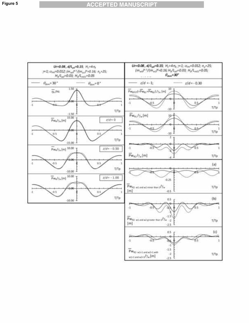
3.2.�Effects�of�wave�direction��
On the left side of Figure 5, the nonlinear water surface and wave pressure in the time domain are compared; it considers wave groups that are approaching the structure orthogonally ( 0�dom� , dotted lines) and those that advance at an angle of 303 with respect to the Y-axis ( 3� 30dom� , solid lines). The theoretical time series are relative to a water depth 0/ pLd of 0.15 with an Ursell number of 0.08. They were computed
assuming that the exceptionally high crest CH of R occurs at time instant 0�T at
the point 00 �� Xx .
The comparison reveals that the directionality does not influence the behavior of the surface displacement. With the nonlinear wave pressure, the directionality is mainly responsible for the disappearance of the humped profiles, with the occurrence of the local minimum at 0�T . When the dominant wave direction has an absolute value greater than zero, the highest maximum of the nonlinear pressure appears at
0�T , in phase with the occurrence of the highest crest of the surface waves at the seawall.
Comparing the right-hand side of Figure 5 with the left-hand side of Figure 4, we can observe that the main contribution to the overall solution is also given in this case by the terms due to the elementary harmonics with 14w . With respect to 0�dom� , for increasing values of |�dom|, the two positive maxima before and after T = 0 in the terms for both the self-interaction of the superharmonics and the interaction between the sub- and superharmonics tend to vanish, thus causing the disappearance of the humped trends in the nonlinear wave pressure. In contrast, the maximum of the nonlinear wave pressure, even if it is in phase with the largest linear pressure and with the highest crest of the surface waves, does not vary in value.
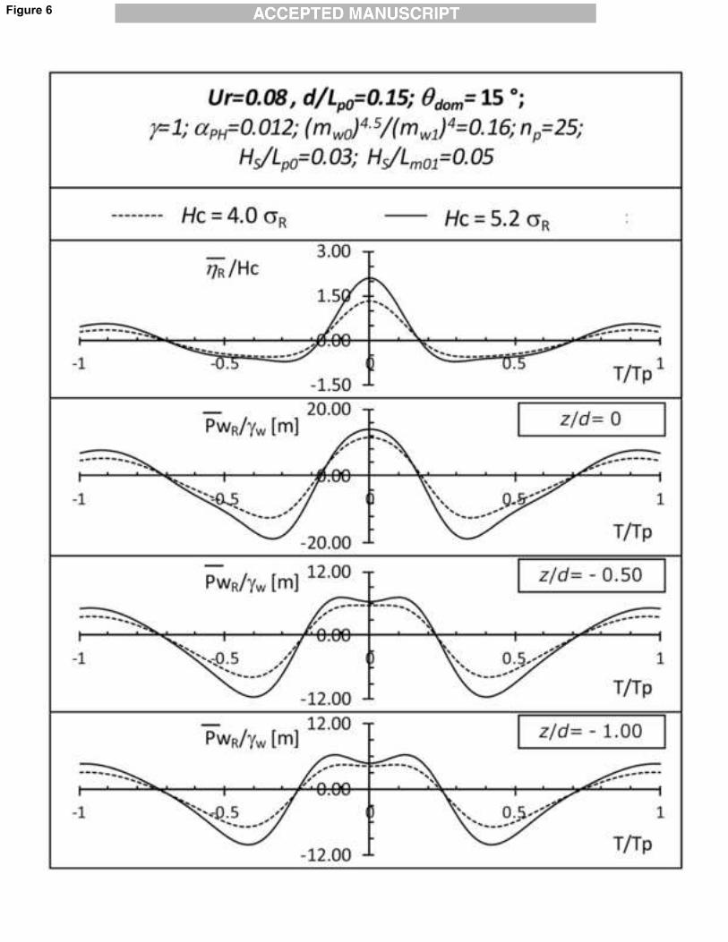
Finally, it is well known that nonlinear effects are amplified for larger wave steepnesses. It is interesting to observe that for a nonzero dominant wave direction and fixed wave conditions, when the high crest CH of the surface waves at the seawall
increases, the nonlinear effects on both the surface displacement and the wave pressure are more remarkable. At 15.0/ 0 �pLd with 3� 15dom� , when CH goes
from R�0.4 to R�2.5 (Figure 6), the steepness of the highest waves in the time domain is increased by 50%. Furthermore, the positive and negative peaks of the nonlinear wave pressure at the bottom depth are enlarged by about 40%. Moreover, with fixed wave conditions, the occurrence at the seawall of a sea wave with greater steepness also deforms the nonlinear pressure profiles, and humped trends appear, even though the dominant wave direction is not zero. For example, when CH is
R�2.5 , the maximum wave pressure at the bottom appears at pT12.0 , after the
occurrence at 0�T of the highest crest of the surface waves, and the pressure at 0�T is 0.75 times the largest pressure value.
4. Validation of nonlinear theory with a small-scale field experiment
4.1. Description of experiment
The nonlinear theory proposed here for sea wave groups interacting with a vertical seawall was validated in a small-scale field experiment conducted at the NOEL in Reggio Calabria (Italy). In this laboratory, located on the waterfront of Reggio Calabria on the east coast of the Strait of Messina, experiments can be performed directly in the sea using techniques associated with the laboratory tanks (Boccotti et al. [50,51,52], Boccotti [30]).
The experimental configuration is presented in Figure 7. A small fully reflective upright seawall with a frame set in reinforced concrete was built. The structure, which consisted of nine caissons, had a total length of 16.2 m and a height of 3.0 m, and was placed at a depth of 1.9 m with respect to the mean water level (MWL). Sixteen pressure transducers were placed on the sea-beaten side along the vertical cross section of the central caisson forming the seawall to measure the fluctuation in the wave pressure acting on it. The incident waves (in the undisturbed field) were evaluated using two ultrasonic probes and two pressure transducers. One of each instrument was assembled on a thin pile with a diameter of 0.05 m and was positioned 13 m from the seawall.
Each gauge recorded continuously for 5 min at a sampling rate of 10 Hz. Among the records, only those of pure wind waves without overturning or breaking waves were considered in the present analyses. In all, there were 94 records, which were characterized by the following wave conditions: significant wave height sH in the
undisturbed field between 0.21 m and 0.41 m, and peak period pT between 1.9 s and
2.7 s. Thus, the relative water depth was
32.0/16.0 0 �� pLd . (4.1)
The considered records represent, in a hydraulic Froude similitude, a small-scale model of sea states during severe storms. Because of the change in the MWL caused by the tide, the water depth d ranged from 1.76 m to 1.95 m. The dominant wave direction dom� had a range of [-93, 153] and was positive when clockwise with respect to the normal outward from the structure.
In the analyzed records, the spectral shape in the frequency domain was evaluated
using Boccotti’s *5 parameter (Boccotti [28,30]), defined as
)0()( *
*
555 T
� , (4.2)
which is the quotient of the absolute value of the first minimum, which occurs at *TT � , and the maximum of the autocovariance function
��� )()()( TttT 5 , (4.3)
where � )(tf defines the mean value of )(tf .
The values of *5 range from 0 to 1: it is 1 for an infinitely narrow spectrum, 0.73 for a mean JONSWAP spectrum, and 0.65 for a Pierson–Moskowitz spectrum.
In the 94 records that were considered, *5 was within )0.76 ,65.0( at the surface, and the Ursell number varied from 0.08 to 0.01.
For obtaining the directional spectrum from sea states recorded at sea near the coast, the method proposed by Boccotti et al. [53] was considered.
4.2. Comparison of theoretical and experimental results
The 94 records considered for validation of the theory are identified by a full sea wave reflection by the seawall, and by the resulting pattern of standing wave groups close to the structure.
In this section, the nonlinear theory is tested by considering as input in the theoretical computations the values of the wave parameters, such as the significant wave height sH , peak period pT , tide level, dominant wave direction dom� , and
relative water depth 0/ pLd , for the record being compared. Regarding the theoretical
directional spectrum, the JONSWAP–Mitsuyasu spectrum is assumed, with spectral
shape parameters + [Eq. (3.2)] such that the parameter *5 related to the theoretical spectrum is equal to that of the considered records.
The theory can be applied when either an exceptionally high crest CH or trough
TH amplitude of the surface displacement occurs. Assuming an exceptionally high crest elevation CH occurs, the nonlinear surface displacement is evaluated as
Similar laws regulate the nonlinear velocity potential and nonlinear wave pressure. It is noteworthy that a positive (absolute maximum) or negative (absolute
minimum) peak of the wave pressure at the bottom of the seawall may be produced by the occurrence on the surface of either an exceptionally high crest amplitude CH or trough amplitude TH of the surface displacement.
Figures 9–13 present a number of comparisons between the analytical and experimental results. In each figure, the lower panels represent the wave pressure in the time domain at the depth of the pressure transducers assembled along the cross section of the tested seawall (Figure 7); the dots are the measurements given by the gauges, and the solid lines are the theoretical profiles, which are exact to the second-order. The second-order analytical profiles were computed by assuming the occurrence of either an extreme wave crest CH or wave trough TH of the surface displacement [Eq. (4.4) or (4.5)], such that the absolute maximum (or minimum) of the analytical wave pressure at the bottom depth is equal in value to that recorded by gauge n.6. The instants of the wave crests of the surface waves at the structure were identified by the signals transmitted by the upper pressure transducers. Therefore, in Figures 9–13, only the theoretically computed nonlinear water elevation is shown. Moreover, the recorded wave force per unit length at the midsection of the structure, which is computed by integrating the measured wave pressures at different water depths, is represented in the upper panels by dots. The theoretical wave force (upper panels, solid line) is computed by considering the following. i) During the crest elevation phase of the water surface, a linear trend was assumed between the total wave pressure up to the second-order at the MWL and the nonlinear wave elevation of the free-surface displacement. ii) During the trough amplitude phase of the water surface, the pressure was assumed to be equal to the hydrostatic pressure if it was greater than the nonlinear wave pressure.
Figure 8 shows the ratios of the absolute maximum and minimum values of both the wave force acting on the seawall and the wave pressure at the bottom depth for each of the 94 analyzed records. The experimental results confirm that the wave pressure at the seawall is a strongly asymmetric process, with the greatest minima significantly exceeding the highest maxima. For all the records, which were characterized by different water conditions, the positive peaks of the wave pressure are 20%–50% smaller than the negative ones, in full agreement with the predictions of
the nonlinear theory. On the other hand, the ratio between the positive and negative peaks of the wave force process ranged from 1.36 to 0.64.
Figures 9, 10, and 11 show the experimental records in which the three highest positive peaks of the wave pressure process
at the bottom depth,
66/
wpwp � , appear,
where 6wp� is the standard deviation of the wave pressure 6wp recorded at the
bottom depth by gauge n.6. Figures 12 and 13 refer to the first two negative peaks of the
66/
wpwp � process.
For the comparisons shown in Figures 9, 10, and 11, the theory was applied by assuming that an exceptionally high crest CH of R [Eq. (4.4)] occurs at time instant
t = 0 at the structure. Records 1, 2 and 3, which are analyzed in Figures 9–11, respectively, are almost homogeneous in terms of the wave characteristics except for the dominant wave direction, which is null for records 1 and 3, and greater than zero for record 2 (see Table 2). The recorded time series in Figures 9–11 are centered
)0( �t at the time instant of the maximum elevation measured at the seawall on the surface. To compare the analytical and experimental results, we supposed at the same time instant that an exceptionally high crest CH in the theoretical nonlinear surface displacement occurred (that is, CH equal to 4.54 R� , 3.84 R� , and 5.12 R� for records 1, 2, and 3, respectively, where R� is the standard deviation of the measured surface waves at the seawall).
As predicted by the nonlinear theory (see Figures 2 and 5), when the wave groups approach the structure orthogonally (the dominant wave direction dom� is null), the greatest maximum of the wave pressure beneath the MWL is out of phase with respect to the highest elevation on the surface, at which a local minimum of the wave pressure occurs. This phenomenon can be clearly seen in records 1 and 3 (the dots in Figures 9 and 11). If we focus on the recorded wave pressure at the bottom depth (gauge n.6), we find that the process is very asymmetric, with the highest maximum being about 0.82 times the greatest minimum in record 1 and about 0.73 times the greatest minimum in number 3. The difference between the positive peak of the wave pressure and the wave pressure at the time instant of the highest elevation at the surface is quite important; in records 1 and 3, the positive peak exceeds the pressure at time instant
0�t by about 56% and 87%, respectively. The theory up to the second-order (the solid lines in Figures 9 and 11) shows very good agreement with the experimental data in terms of both trends and values near the occurrence of the exceptionally high crest of water displacement. The theory can fully describe the main phenomena under the MWL, namely, the drop in pressure at 0�t and the highest maximum being out of phase with the maximum elevation at the surface. Above the MWL, a number of differences appear between the predictions of the highest elevation and the
experimental data; in this case, the theoretical results are more conservative with regard to positive extreme values.
In record 2, even though it is characterized by an Ursell number smaller than those in records 1 and 3, the wave groups show a direction of advance equal to 83 with respect to normal to the seawall. According to the nonlinear theory, the recorded wave pressure profiles under the MWL are smooth, without the formation of two humps (the dots in Figure 10). The absolute maximum of the recorded wave pressure is in phase with the maximum water elevation along the cross section of the seawall. The wave pressure describes a peculiar asymmetry with greater minima in this case as well; at the bottom (gauge n.6), the ratio between the positive and negative peaks of the measured wave pressure is equal to 0.73. The nonlinear theory (the solid lines in Figure 10) fully agrees with the experimental data, as it can describe all the results highlighted here.
Figures 12 and 13 present analyses of the records in which the greatest negative peaks of the wave pressure at the bottom (gauge n.6) appeared during the experiment. The records are centered (t = 0) at the time instant at which the greatest minimum of the wave pressure at the seawall at the bottom depth occurred. In our application of the nonlinear theory, we have supposed at the same time instant that an exceptionally high trough HT of the theoretical nonlinear surface displacement occurred (that is, TH equal to 3.74 R� and 4.0 R� for records 4 and 5, respectively, where R� is the standard deviation of the measured surface waves at the seawall). In records 1, 2, and 3, the asymmetry of the wave pressure profiles is enhanced. The depths of the deepest troughs are about twice as large as the heights of the highest crests of the wave pressure in records 4 and 5.
Figure 12 considers record 4 of Table 2, which was identified as having one of the lowest Ursell numbers recorded during the experiment and a dom� close to zero. From the signals of the highest gauges (dots in Figure 12), we recognize the appearance of two crests of surface waves at the seawall at time instants pTt 43.0��
and pTt 48.0� , respectively, for gauge n.17. These times are before and after the
occurrence of the deepest trough of the surface waves, which is fixed at time instant 0�t . For each of these wave crests on the surface, the formation of humped wave
pressure profiles is observed at the lower gauges, with the positive peaks being out of phase with the highest elevation of the upper gauges. For gauge n.6, these peaks occur at pT61.06 , and the drop in the positive pressure is quite important: the ratio between
the greatest positive pressure (at pTt 61.06� ) and the positive pressure at the time of
the highest crest of the surface waves is about 2.6 in both cases. The theory up to the second-order (the solid lines in Figure 12) describes the characteristics of the record
well in terms of both the positive and negative peaks of the wave pressure in a process characterized by asymmetry.
The last record is characterized by a narrower frequency spectrum compared to
the other considered records ( 71.0* �5 for the incident surface waves) and by the greatest �dom recorded during the experiment, which is equal to 15°. By considering two crests of surface waves (see gauge n.17) that appeared before and after the occurrence of the deepest trough of the wave pressure at the bottom (gauge n.6), we observe that the highest maxima above the MWL are approximately in phase with the greatest maxima beneath the MWL (dots in Figure 13), displaying roughly round wave pressure profiles. The theoretical nonlinear results (solid lines in Figure 13) captured all of these main features, although they sometimes underestimated the positive peaks above the MWL.
Finally, the upper panel of Figure 14 shows, for every record in the experiment, the ratio between the wave pressures recorded by gauges n.12 and n.6 at time instant t, when the highest maximum of the wave pressure at gauge n.12 (located above the MWL) occurs. The lower panel shows the ratio between the maximum positive wave pressures recorded by gauges n.12 and n.6 (the two maxima may occur at different time instants, depending upon the wave conditions). These behaviors confirm the distinct phenomenon predicted by nonlinear theory in Table 1, namely, that the strong reduction in wave pressure at the bottom depth corresponds to the appearance of the greatest positive peak on the surface when the dominant direction of advance of the wave groups is zero, whereas under the same conditions, the absolute positive maxima varies gradually along the cross section of the seawall. This effect is enhanced as the relative water depth increases. For example, at 3.0/ 0 �pLd , the highest maximum
recorded at gauge n.12 was 6.2 times the positive pressure recorded at the same time instant at the bottom and 2.5 times the highest maximum recorded at gauge n.6. This trend is distinct for 0�dom� . For increasing values of || dom� , the quotient of the highest positive maximum on the surface remains steady at about twice the quotient recorded at the bottom. This parameter is roughly equal in value if we consider the variation in the absolute maxima along the cross section of the seawall (see both panels in Figure 14). This confirms that, for all the data collected during the experiment when dom� differs from zero, the greatest positive maximum at the bottom is in phase with the highest positive maximum on the surface.
5. Conclusions
In this paper, an analytical closed-form solution was derived up to the second-order for three-dimensional wave groups that are fully reflected by an upright seawall.
The theory reveals that the second-order contributions strongly affect the mechanics of wave groups for both surface waves and pressure head waves when an exceptionally high crest or deep trough of the free-surface displacement process impacts the structure.
Classical second-order effects on the free-surface elevation were found, with an increase in the heights of the highest crests and a reduction in the depth of the deepest troughs with respect to those predicted by linear theories and a significant asymmetry in which the crests exceed the troughs. These effects are more important for the reflection of wave groups than for those observed in an undisturbed field because the free-surface displacement is amplified at a seawall.
In particular, this paper focuses on the wave pressures at which the nonlinearity produces more distinctive results. The second-order theory shows that the deepest troughs are much deeper than those obtained in the linear results, exhibiting an important asymmetry between the extreme maxima and minima, with the minima markedly exceeding the maxima. Moreover, a distinctive behavior of nonlinearity in the time series of the wave pressure occurs when the extreme crests of the water surface impact the seawall. The theory reveals the occurrence of two positive peaks of the wave pressure or wave force out of phase with the maximum elevation at the surface, at which a drop in the pressure appears with the local minimum. The theory proves that the three-dimensionality of wave groups, both the directional spreading function and the dominant direction of the incident wave spectrum, is mainly responsible for the described characteristic second-order trends in the wave pressure.
The nonlinear theory was finally tested through a small-scale field experiment conducted at a vertical seawall at the NOEL in Reggio Calabria (Italy). The experimental records cover a wide range of wave conditions, with different values of water depth, Ursell number, wave steepness, and directional spreading function. A number of widely varying wave conditions were analyzed, demonstrating the occurrence at sea of the time series of the wave pressure corresponding to the main distinctive phenomena described by the theory. Comparisons of the theoretical and experimental data showed good agreement. Therefore, it has been proved that most of the different behaviors that characterize the inhomogeneous wave field of very high wave groups in reflection can be associated with the effects of nonlinearity, and that they can be described well by the proposed nonlinear theory.
The closed-form solution of the velocity potential up to the second-order allows us to obtain the second-order component of the deterministic surface displacement
2R ,
which may also be obtained using either the KSBC [Eq. (2.11)] or DSBC [Eq. (2.12)]. The closed solution for
2R is given by
)/(d d d d )}]cos()cos(A
)cos([A)-]cos()cos(A)cos({[A
)cos()cos(),(),(
2),(
12122121
21212121
21220 0
2
0
2
0114
2
00
2
121
2
g
SSH
TtxR
CR X
�����
������
�
�
���
� �
� � � ���
��������
��������
�������
� �
(A.1)
as a function of the interaction kernels of the nonlinear surface displacement, which are defined as
������
������
��
�
��
nnn
nnn
gg
n
gg
BD),,,(A
2,1
BD),,,(A
12
11
12121
12
11
12121
������
������
(A.2)
with coefficients �nD (n = 1,2) expressed by
2,1
)(])1(cos[
)1( ),,,(D
3)(])1(cos[
)1( ),,,(D
212
212121
212
2121
212
212121
212
2121
�
�������
�������
�
�
n
kkg
kkg
nn
nn
n
n
��������
����
��������
����
(A.3)
and coefficients �n
B (n = 1,2) [Eqs. (2.24)] introduced for the definition of R2� .
A.2.�Solution�for�the�� parameter���
Assuming that the deterministic surface elevation is a zero mean process of time (according to Whitham [45] and Longuet-Higgins [20]), the corresponding deterministic velocity potential cannot at the same time be a zero mean process in time. For a wave field in reflection, it has to have at least one term that is proportional to T because the boundary condition at the seawall (Eq. 2.16) cannot allow for the definition of a term proportional to Y. The parameter � is derived by imposing the principle of mass conservation for a fixed volume piercing the water surface that extends infinitely into deep water and is bounded by the seabed, the rigid seawall in
finite water, and two vertical planes orthogonal to the seawall. This leads to the following relation:
,d d d d),,,(),(),(
21212212122
0 0
2
0
2
0114
2
�������������
� �
FSSHgR
C � � � �� �
��� (A.4)
where
*&
*'
(
77
���
. and if 0
and if )(cos )2sinh(
2),,,(
2121
212112
1
1
2121
����
��������� dk
kF (A.5)
With the derivation of � , the solutions given by Eq. (A.1) for 2R and by Eq.
(2.22) for 2R��completely satisfy the partial differential system of equations [Eqs.
(2.10), (2.11), (2.12), (2.15), (2.16)] that govern the problem being examined.
APPENDIX B
The j-th moment jm is
��
�0
d )( ��� Em jj , (B.1)
which, assuming the JONSWAP frequency spectrum in the dimensionless form (3.2), can be expressed as
jPH w
jpj mgm ��� 42�� , (B.2)
where jwm is the dimensionless moment:
��
���
*�
*��
*&
*'(
!
"#$
% ����
02
245 d
2)1(explnexp)25.1exp( wwwwm j
w j �+ . (B.3)
Thus, through Eqs. (B.2) and (B.3), the mean wave period 01mT (3.8) is made explicit
as
1
001
w
wpm m
mTT � , (B.4)
and the following general relation between the significant wave height sH and the peak period )/2( ppT ��� is introduced:
5.022 )(0wps mTgH PH�� �� , (B.5)
by means of which the Ursell number can be stated as given by Eq. (3.9).
R E F E R E N C E S
[1] W.S. RAYLEIGH, Deep water waves, progressive or stationary, to the third order of approximation, Proc. R. Soc. London, Ser. A 91 (1915), pp. 345.
[2] W.G. PENNEY, A.T. PRICE, Finite periodic stationary gravity waves in a perfect fluid Part II, Philos. Trans. R. Soc. London, Ser. A 244 (882) (1952), pp. 254–284.
[3] G.I. TAYLOR, An experimental study of standing waves, Proc. R. Soc. London, Ser. A 218 (1953), pp. 44–59.
[4] D. FULTZ, An experimental note on finite-amplitude standing gravity waves, J. Fluid Mech. (13) (1962), PP. 193–212.
[5] R.D. EDGE, G. WAITERS, The period of standing gravity waves of largest amplitude on water, J. Geophys. Res. 69 (1964), pp. 1674–1675.
[6] I. TADJBAKHSH, J.B. KELLER, Standing surface waves of finite amplitude, J. Fluid Mech. 8 (1960), pp. 442–451.
[7] Y. GODA, The fourth order approximation to the pressure of standing waves, Coast. Eng. Jpn. 10 (1967), pp. 1–11.
[8] L.W. SCHWARTZ, J.D. FENTON, Strongly nonlinear waves, Ann. Rev. Fluid Mech., 14 (1982), pp. 39–60.
[9] L.W. SCHWARTZ, A.K. WHITNEY, A semi-analytic solution for nonlinear standing waves in deep water, J. Fluid Mech., 107 (1981), pp. 147–171.
[10] J.-M. VANDEN-BROECK, L.W. SCHWARTZ, Numerical calculation of standing waves in water of arbitrary uniform depth, Phys. Fluids, 24 (1981) , pp.812–815.
[11] J.-M. VANDEN-BROECK, Nonlinear gravity-capillary standing waves in water of arbitrary uniform depth, J. Fluid Mech., 139 (1984),,pp. 97–104.
[12] R. MARCHANT, A.J. ROBERts, Properties of short-crested waves in water of finite depth, J. Aust. Math. Soc. B, 29 (1987), pp. 103.
[13] G.N. MERCER, A.J. ROBERTS, Standing waves in deep water: their stability and extreme form, Phys. Fluids A, 4 (1992), pp. 259–269.
[14] G.N. MERCER, A.J. ROBERTS, The form of standing waves on finite depth water, Wave Motion, 19 (1994), pp. 233–244.
[15] C.-P. TSAI, D.-S. JENG, Numerical Fourier solutions of standing waves in finite water depth, Appl. Ocean Res., 16 (1994), pp. 185–193.
[16] W.W. SCHULTZ, J.-M. VANDEN-BROECK, L. JIANG, M. PERLIN, Highly nonlinear standing water waves with small capillary effect, J. Fluid Mech., 369 (1998), pp. 253–272.
[17] Q. ZHU, Y. LIU, K.P. DICK, D.K.P. YUE, Three-dimensional instability of standing waves, J. Fluid Mech., 496 (2003), pp. 213–242.
[18] L. JIANG, C.-L. TING, M. PERLIN, W.W. SCHULTZ, Moderate and steep Faraday waves: instabilities, modulation and temporal asymmetries, J. Fluid Mech., 329 (1996), pp. 275–307.
[19] L. JIANG, M. PERLIN, W.W. SCHULTZ, Period tripling and energy dissipation of breaking standing waves, J. Fluid Mech., 369 (1998), pp. 273–299.
[20] M.S. LONGUET-HIGGINS, On the form of the highest progressive and standing waves in deep water, Proc. R. Soc. London, Ser. A, 331 (1973), pp. 445–456.
[21] M.S. LONGUET-HIGGINS, Vertical jets from standing waves, Proc. R. Soc. London, Ser. A, 457 (2001), pp. 495–510.
[22] M.S. LONGUET-HIGGINS, D.G. DOMMERMUTH, On the breaking of standing waves by falling jets, Phys. Fluids, 13 (2001), pp. 1652–1659.
[23] M.S. LONGUET-HIGGINS, D.G. DOMMERMUTH, Vertical jets from standing waves. II, Proc. R. Soc. London, Ser. A, 457 (2001), pp. 2137–2149.
[24] M.S. LONGUET-HIGGINS, D.A. DRAZEN, On steep gravity waves meeting a vertical wall: A triple instability, J. Fluid Mech., 466 (2002), pp. 305–318.
[25] M.S. LONGUET-HIGGINS, E.D. COKELET, The deformation of steep surface waves on water. I. A numerical method of computation, Proc. R. Soc. London, Ser. A, 358 (1976), pp. 1–26.
[26] M.J. COOKER, D.H. PEREGRINE, Pressure impulse theory for liquid impact problems, J. Fluid Mech., 297 (1995), pp. 193–214.
[27] D.H. PEREGRINE, Water-wave impact on walls, Ann. Rev. Fluid Mech., 35 (2003), pp. 23–43.
[28] P. BOCCOTTI, On ocean waves with high crests, Meccanica, 17 (1982), pp. 16–19.
[29] P. BOCCOTTI, Quasi-determinism of sea wave groups, Meccanica, 24 (1989), pp. 3–14.
[30] P. BOCCOTTI, Wave Mechanics for Ocean Engineering. Elsevier Science, New York (2000).
[31] O.M. PHILLIPS, D. GU, M. DONELAN, On the expected structure of extreme waves in a Gaussian sea, I. Theory and SWADE buoy measurements, J. Phys. Oceanogr. 23 (1993), pp. 992–1000.,
[32] O.M. PHILLIPS, D. GU, E.J. WALSCH, On the expected structure of extreme waves in a Gaussian sea, II. SWADE scanning radar altimeter measurements, J. Phys. Oceanogr., 23
(1993), pp. 2297–2309.
[33] G. LINDGREN, Some properties of a normal process near a local maximum, Ann. Math. Stat., 41 (1970), pp. 1870–1883.
[34] G. LINDGREN, Local maxima of Gaussian fields, Ark. Mat., 10 (1972), pp. 195–218.
[35] J.N. SHARMA, R.G. DEAN, Second-order directional seas and associated wave forces, Soc. Pet. Eng. J., 4 (1981), pp. 129.
[36] J.F. DALZELL, A note on finite depth second-order wave-wave interactions, Appl. Ocean Res., 21 (1999), pp. 105.
[37] F. ARENA, On non-linear very large sea wave groups, Ocean Eng., 32 (2005), pp. 1311–1331. DOI:10.1016/J.OCEANENG.2004.12.002
[38] F. FEDELE, F. ARENA, Weakly nonlinear statistics of high random waves, Phys. Fluids, 17
(2005), pp. 026601-1, 026601-10 .
[39] F. ARENA, A. ASCANELLI, V. NAVA, D. PAVONE, A. ROMOLO, Non-linear three-dimensional wave groups in finite water depth, Coastal Eng., 55 (2008), pp.1052–1061. doi:10.1016/j.coastaleng.2008.04.002
[40] J.J. JENSEN, Conditional second-order short-crested water waves applied to extreme wave episodes, J. Fluid Mech., 545 (2005), pp. 29–40.
[41] P. BOCCOTTI, A general theory of three-dimensional wave groups. Part I: the formal derivation. Part II: interaction with a breakwater, Ocean Eng., 24 (1997), pp. 265–300.
[42] A. ROMOLO, F. ARENA, Mechanics of nonlinear random wave groups interacting with a vertical wall, Phys. Fluids, 20 (2008), pp.036604-1, 036604-16, DOI: 10.1063/1.2890474.
[43] P. BOCCOTTI, On the highest waves in a stationary Gaussian process, Atti Accad. Ligure Sci. Lett., Genoa, 38 (1981), pp. 271.
[44] F. Arena, Interaction between long-crested random waves and a submerged horizontal cylinder, Phys. Fluids, 18 (2006), pp. 076602.
[45] G.B. WHITHAM, Linear and Nonlinear Waves. Wiley, New York (1974).
[46] K. HASSELMANN, T.P. BARNETT, E. BOUWS, H. CARLSON, D.E. CARTWRIGHT, E. ENKE, J.A. EWING, H. GIENAPP, D.E. HASSELMANN, P. KRUSEMANN, A. MEERBURG, P. MÜLLER, D.J. OLBERS, K. RICHTER, W. SELL, H. WALDEN, Measurements of wind-wave growth and swell decay during the Joint North Sea Wave Project (JONSWAP), Dtsch. Hydrogr. Z. A, 12 (1973), pp. 1–95.
[47] H. MITSUYASU, F. TASAI, T. SUARA, Observation of directional spectrum of ocean waves using a clover-leaf buoy, J. Phys. Oceanogr., 5 (1975), pp. 750–760.
[48] W.J. PIERSON, L.A. MOSKOWITZ, A proposed spectral form for fully developed waves based on the similarity theory of S. A. Kitaigorodskii, J. Geophys. Res., 69 (1964), pp. 5181–5190.
[49] F. ARENA, D. PAVONE, The return period of non-linear high wave crests, J. Geophys. Res. , 111 (2006) C8, paper C08004, doi: 10.1029/2005JC003407.
[50] P. BOCCOTTI, G. BARBARO, L. MANNINO, A field experiment on the mechanics of irregular gravity waves, J. Fluid Mech., 252 (1993), pp. 173–186.
[51] P. BOCCOTTI, G. BARBARO, V. FIAMMA, L. MANNINO, A. ROTTA, An experiment at sea on the reflection of the wind waves, Ocean Eng., 20 (1993), pp. 493–507.
[52] P. BOCCOTTI, F. ARENA, V. FIAMMA, A. ROMOLO, G. BARBARO, Small�scale field experiment on wave forces on upright breakwaters, J. Waterway Port Coastal Ocean Eng., 138 (2) (2012), pp. 97-114, doi: 10.1061/(ASCE)WW.1943-5460.0000111.
[53] P. BOCCOTTI, F. ARENA, V. FIAMMA, A. ROMOLO, G. BARBARO, Estimation of mean spectral directions in random seas, Ocean Engineering, 38 (2011), pp. 509–518, doi:10.1016/j.oceaneng.2010.11.018.
TABLES
TABLE 1. Ratio between nonlinear wave pressure at 3.0/ ��dz and that at 1/ ��dz at
time instant 0�T when the greatest elevation on the surface occurs at the seawall, and at the
time instant of the absolute maximum of the pressure (for the quantities, also see the uppermost
panels in Figure 3).
TABLE 2. Wave field conditions of the five experimental records during which the greatest
representing nonlinear energy transfer between elementary harmonics for 1/ ��dz and
3.0/ ��dz . The theoretical time series assume that an exceptionally high crest HC of the
surface displacement R occurs at time instant 0�T at 00 �� Xx .
FIGURE 6. Effects associated with an increase in wave steepness for fixed wave conditions:
16.0/ 0 �pLd , 08.0�rU , 3� 15dom� , with a Pierson–Moskowitz–Mitsuyasu directional
wave spectrum. The height of the exceptionally high crest HC of the surface displacement R
occurring at time instant 0�T at 00 �� Xx is R�0.4 or R�2.5 .
FIGURE 7. Schematic of field experiment conducted at sea at Reggio Calabria in the NOEL
laboratory. Three-dimensional plan (a) and section (b) of the reflective seawall employed for the
experiment. Maps of the gauges located at the structure (b) and on the piles in an undisturbed
field (c) are also shown.
�
FIGURE 8. Ratio between absolute maximum and minimum of measured wave force wF
(upper panel) and measured wave pressure at the bottom depth 6wp (lower panel) for each of
the 94 experimental records.
�
FIGURE 9. Record 1 in Table 2. The recorded time series (dots) are centered at the time instant of
the highest elevation on the surface at the seawall. The theoretical second-order wave pressure
(solid lines) is computed at every depth assuming that, at the previous time instant, an
exceptionally high crest )54.4( RCH �� of the surface displacement occurred at the structure.
�
FIGURE 10. Record 2 in Table 2. The recorded time series (dots) are centered at the time instant
when the absolute maximum of the measured wave pressure occurs at the bottom. The
theoretical second-order wave pressure (solid lines) is computed at every depth assuming that, at
the same time instant, an exceptionally high crest )84.3( RCH �� of the surface displacement
occurs at the structure.
�
FIGURE 11. Record 3 in Table 2. The recorded time series (dots) are centered at the time instant
of the highest elevation on the surface at the seawall. The theoretical second-order wave
pressure (solid lines) is computed at every depth assuming that, at the previous time instant, an
exceptionally high crest )12.5( RCH �� of the surface displacement occurs at the structure.
�
FIGURE 12. Record 4 in Table 2. The recorded time series (dots) are centered at the time instant
when the absolute minimum of the measured wave pressure occurs at the bottom. The
theoretical second-order wave pressure (solid lines) is computed at every depth assuming that, at
the same time instant, an exceptionally deep trough )74.3( RTH �� of the surface
displacement occurs at the structure.
�
FIGURE 13. Record 5 in Table 2. The recorded time series (dots) are centered at the time instant
when the absolute minimum of the measured wave pressure occurs at the bottom. The
theoretical second-order wave pressure (solid lines) is computed at every depth assuming that, at
the same time instant, an exceptionally deep trough )4( RTH �� of the surface displacement
occurs at the structure.
�
FIGURE 14. Upper panel: ratio between maximum positive wave pressure recorded by gauge
n.12, which occurs at time instant t , and wave pressure recorded by gauge n.6 at time instant t
. Lower panel: ratio between maximum positive wave pressures recorded by gauges n.12 and
n.6 (the two maxima may occur at different time instants, depending on the wave conditions).
�
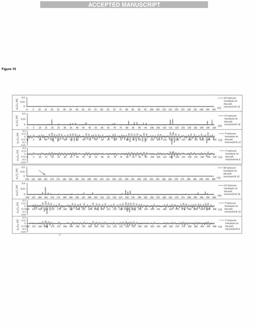
FIGURE 15. Time series of wave pressure at the seawall recorded in the sea during the small-
scale experiment: the entire record with the deepest trough is from Figure 12.
�
A nonlinear theory is given for the 3D sea wave groups interacting with a seawall The solution gives free surface displacement and velocity potential to the 2nd order The theoretical results are validated with a small-scale field experiment The experiment was carried out in the Natural Ocean Engineering Laboratory (Italy) �