Three Dimensional Plots of Smoothed Bivariate Distributions

• Smoothing using Rectangular Kernel

• Preparing Data for Import to Mathematica

• Starting and Using Mathematica

• Importing Data

• Three-D Surface Plots

• Animations

Smoothed Bivariate Distribution

• First we'll simulate some data.

tX <- c(rnorm(150, mean=10, sd=5), rnorm(50, mean=0, sd=2))

tY <- 5 + .5 * tX + rnorm(200,mean=0,sd=2)

smoothX <- seq(-5, 25, by=2)

smoothY <- seq(-5, 25, by=2)

smoothF <- matrix(NA, length(smoothX), length(smoothY))

h <- 5

for (i in 1:length(smoothX)) {

x <- smoothX[i]

t1x <- abs(x - tX)/h

for (j in 1:length(smoothY)) {

y <- smoothY[j]

t1y <- abs(y - tY)/h

t2 <- rep(0, length(t1x))

t2[t1x < 1 & t1y < 1] <- 1/2

smoothF[i,j] <- sum(t2)/(length(tX)*h)

}

}

smoothF <- smoothF/sum(smoothF)

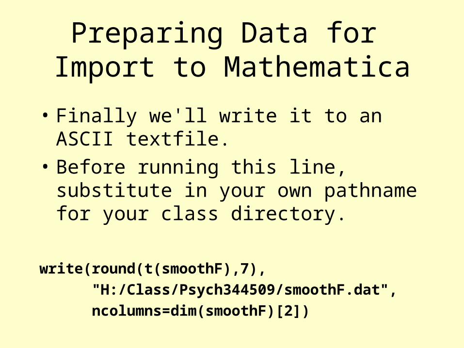
Preparing Data for Import to Mathematica

• Finally we'll write it to an ASCII textfile.

• Before running this line, substitute in your own pathname for your class directory.

write(round(t(smoothF),7),

"H:/Class/Psych344509/smoothF.dat",

ncolumns=dim(smoothF)[2])

Preparing Data for Import to Mathematica

• Now let's look at the data file in PFE

• Open smoothF.dat in PFE

0 0.0006098 0.001626 0.004065 0.0058943 0.0060976 0.0054878 0.0044715 0.0020325 0.0002033 0 0 0 0 0 0

0 0.0006098 0.002439 0.0069106 0.0097561 0.0101626 0.0095528 0.0077236 0.003252 0.0004065 0 0 0 0 0 0

0 0.0006098 0.002439 0.0077236 0.0113821 0.0119919 0.0115854 0.0097561 0.0044715 0.000813 0.0002033 0 0 0 0 0

Starting and Using Mathematica

• Locate and start Mathematica 4.1 in the Program Menu.

• There will be an new “notebook” waiting.

• Type 2+2; and press the Enter key on the keypad.

• The number 4 will appear as output.

• Note that the input and output from the first calculation is delimited by a square bracket on the right.

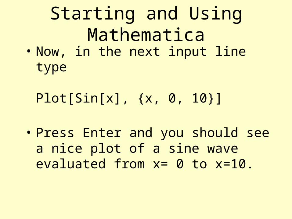
Starting and Using Mathematica

• Now, in the next input line type

Plot[Sin[x], {x, 0, 10}]

• Press Enter and you should see a nice plot of a sine wave evaluated from x= 0 to x=10.

Getting Help in Mathematica• In the next input cell type

?Plot

• Now press Enter and see what happens.

• You can also use the Help Browser.

• Help is arranged by "Packages".

• Some Packages are optional.

Getting Help in Mathematica

• Scroll down the page of help on Plot after clicking on “further examples”.

• You will see example code that you can copy and paste into your notebook.

Saving Your Work in Mathematica

• Choose the menu item File->SaveAs and save your work into your class folder as the filename "Example1".

• Save your work often when using Mathematica as it has a tendency to crash under Windows.

More Help in Mathematica

• In the Help Browser, the left-most column should have Graphics selected.

• In the second column from the left, select 3D Plots.

• In the last column select ListPlot3D.

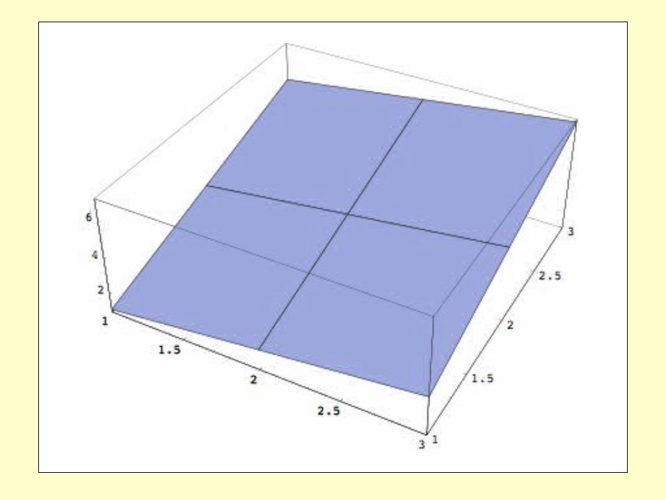
More Help in Mathematica

• Evaluate the example to see a 3D plot.

• Now let’s try a 3D Plot

tMatrix = {{1,2,3}, {3,4,5}, {5,6,7}}

ListPlot3D[tMatrix]

• Type them in and press enter.

Importing Data into Mathematica• Open the file you downloaded at the

beginning of class: ThreeD3.nb• Notice that this file opens in a second

notebook.

• The first input cell of this file should read:<<Graphics`Animation`

• Put your cursor in that cell by clicking anywhere in it and then press Enter.

• This loads the Add-On animation package.

Viewing an Animation• Press enter in the second and third cells.

• You’ll see a lot of graphics being generated.

• These are the cels in an animation.

• Double-Click on one of the cels so that it is selected with a box around it.

• The graphic should start spinning.

• The controls for slowing or speeding the animation are at the bottom of the notebook window.

Importing Data into Mathematica• That was fun, but now let’s get down to

business.

• Click in the next input area after the animated graphics.

• Change the directory to be your class directory.

• Press Enter.

Three-D Surface Plots

• The next cell has a line that reads

ListPlot3D[theData1]

• Put your cursor in that line and press Enter.

• A 3-D projection of the surface we created in Splus will be plotted.

Three-D Surface Plots

• Let’s animate the plot with SpinShow.

• If you change the size of the first graph, it will change the size of the whole animation the next time you press Enter.

Three-D Surface Plots

• There are many options to 3D plotting for changing the perspective view, the hues, etc.

Saving Graphs and Animations

• Click on a graph to select it.

• Select Edit -> Save Selection As

• Notice the options for saving the graphic or animation.

For Tuesday

• Next we'll talk about longitudinal data: time series, recursion visualization and state space plotting.