Three-Dimensional Simulations of Seismic-Wave Propagation in the Taipei Basin with Realistic Topography Based upon the Spectral-Element Method by Shiann-Jong Lee, How-Wei Chen, Qinya Liu * , Dimitri Komatitsch † , Bor-Shouh Huang, and Jeroen Tromp Abstract We use the spectral-element method to simulate strong ground motion throughout the Taipei metropolitan area. Mesh generation for the Taipei basin poses two main challenges: (1) the basin is surrounded by steep mountains, and (2) the city is located on top of a shallow, low-wave-speed sedimentary basin. To accommodate the steep and rapidly varying topography, we introduce a thin high-resolution mesh layer near the surface. The mesh for the shallow sedimentary basin is adjusted to honor its complex geometry and sharp lateral wave-speed contrasts. Variations in Moho thickness beneath Northern Taiwan are also incorporated in the mesh. Spectral- element simulations show that ground motion in the Taipei metropolitan region is strongly affected by the geometry of the basin and the surrounding mountains. The amplification of ground motion is mainly controlled by basin depth and shallow shear-wave speeds, although surface topography also serves to amplify and prolong seismic shaking. Introduction Taipei City in Taiwan is one of the most densely popu- lated metropolitan areas situated on top of a shallow sedi- mentary basin. Over the past 20 yr, seismic disasters in the Taipei metropolitan area, particularly the 21 September 1999 Chi-Chi (M w 7:6) and 31 March 2002 east coast (M L 6:8) earthquakes, have caused significant damage with considerable casualties (e.g., Wen et al., 1995; Wen and Peng, 1998; Chen, 2003). Furthermore, recent studies sug- gest that moderate earthquakes near the basin also have the potential to cause strong ground shaking throughout the city (Lin, 2005). Compared to the Los Angeles basin, the Taipei basin is small, about 20 × 20 km at the surface, and relatively shal- low, with a maximum depth of less than 1000 m. It is surrounded by varied topography, including mountains, tableland, and a volcano group (Fig. 1a), collectively pro- ducing changes in elevation varying between sea level and about 1120 m. There are two major discontinuities in the basin: the SongShan formation and the basin basement (Fig. 1b). The SongShan formation is a shallow, low-shear- wave-speed sedimentary layer. The basin is surrounded by Tertiary basement with a deepest extent of about 700– 1000 m (Wang et al., 2004). Taipei city’ s high-rise buildings, including the world’ s current tallest building Taipei 101 in the eastern part of the basin, make the heavily populated re- gion particularly vulnerable to earthquakes. In recent years, numerical simulations have been suc- cessfully used to study the complex nature of strong ground motion due to earthquakes (see, e.g., Olsen et al., 1995, 1996; Wald and Graves 1998; Komatitsch et al., 2004) and the related seismic hazard (e.g., Olsen, 2000). However, for the Taipei basin, slow, laterally variable sedimentary layers and sharp transitions between shallow sediments and the underlying basement pose a considerable numerical chal- lenge. Furthermore, the notable topography around Taipei city makes the issue even more daunting. Lee, Huang, et al. (2006) used a finite-difference method to assess strong ground motions in the Taipei area for a variety of basin mod- els. However, due to the difficulty of incorporating the free surface condition in the finite-difference method (see for in- stance Robertsson, 1996), surface topography was not con- sidered in their analysis. To accommodate the considerable surface topography as well as the highly variable low-wave-speed sedimentary ba- sin, we will use the spectral-element method (SEM) to simu- late siesmic-wave propagation in the Taipei metropolitan area. The SEM is a numerical technique developed more than * Present address: Institute of Geophysics and Planetary Physics, Scripps Institution of Oceanography, University of California, San Diego, California 92093-0225 † Also at: Institut Universitaire de France, 103 Boulevard Saint-Michel, 75005 Paris, France. 253 Bulletin of the Seismological Society of America, Vol. 98, No. 1, pp. 253–264, February 2008, doi: 10.1785/0120070033
Transcript
Three-Dimensional Simulations of Seismic-Wave Propagation in the
Taipei Basin with Realistic Topography Based upon the
Abstract We use the spectral-element method to simulate strong ground motionthroughout the Taipei metropolitan area. Mesh generation for the Taipei basin posestwo main challenges: (1) the basin is surrounded by steep mountains, and (2) the cityis located on top of a shallow, low-wave-speed sedimentary basin. To accommodatethe steep and rapidly varying topography, we introduce a thin high-resolution meshlayer near the surface. The mesh for the shallow sedimentary basin is adjusted to honorits complex geometry and sharp lateral wave-speed contrasts. Variations in Mohothickness beneath Northern Taiwan are also incorporated in the mesh. Spectral-element simulations show that ground motion in the Taipei metropolitan region isstrongly affected by the geometry of the basin and the surrounding mountains.The amplification of ground motion is mainly controlled by basin depth and shallowshear-wave speeds, although surface topography also serves to amplify and prolongseismic shaking.
Introduction
Taipei City in Taiwan is one of the most densely popu-lated metropolitan areas situated on top of a shallow sedi-mentary basin. Over the past 20 yr, seismic disasters inthe Taipei metropolitan area, particularly the 21 September1999 Chi-Chi (Mw 7:6) and 31 March 2002 east coast(ML 6:8) earthquakes, have caused significant damage withconsiderable casualties (e.g., Wen et al., 1995; Wen andPeng, 1998; Chen, 2003). Furthermore, recent studies sug-gest that moderate earthquakes near the basin also havethe potential to cause strong ground shaking throughoutthe city (Lin, 2005).
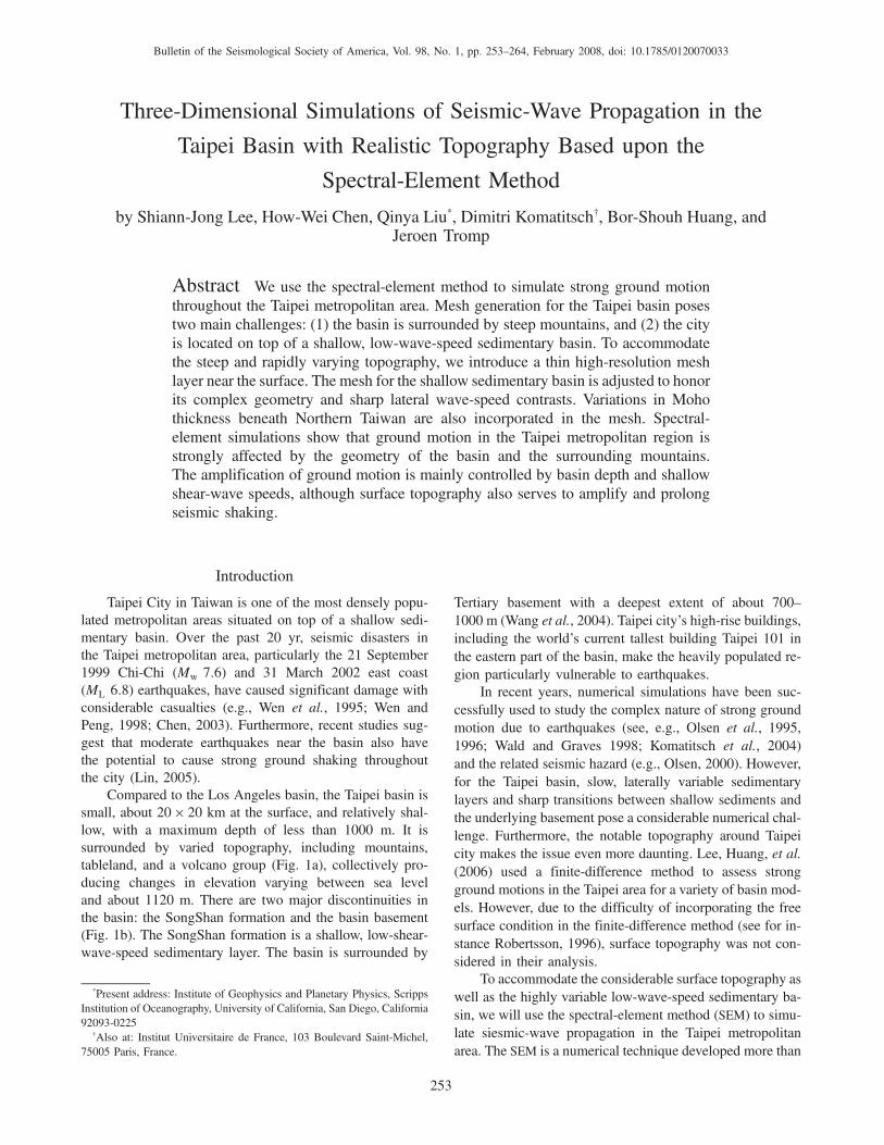
Compared to the Los Angeles basin, the Taipei basin issmall, about 20 × 20 km at the surface, and relatively shal-low, with a maximum depth of less than 1000 m. It issurrounded by varied topography, including mountains,tableland, and a volcano group (Fig. 1a), collectively pro-ducing changes in elevation varying between sea leveland about 1120 m. There are two major discontinuities inthe basin: the SongShan formation and the basin basement(Fig. 1b). The SongShan formation is a shallow, low-shear-wave-speed sedimentary layer. The basin is surrounded by
Tertiary basement with a deepest extent of about 700–1000 m (Wang et al., 2004). Taipei city’s high-rise buildings,including the world’s current tallest building Taipei 101 inthe eastern part of the basin, make the heavily populated re-gion particularly vulnerable to earthquakes.
In recent years, numerical simulations have been suc-cessfully used to study the complex nature of strong groundmotion due to earthquakes (see, e.g., Olsen et al., 1995,1996; Wald and Graves 1998; Komatitsch et al., 2004)and the related seismic hazard (e.g., Olsen, 2000). However,for the Taipei basin, slow, laterally variable sedimentarylayers and sharp transitions between shallow sediments andthe underlying basement pose a considerable numerical chal-lenge. Furthermore, the notable topography around Taipeicity makes the issue even more daunting. Lee, Huang, et al.(2006) used a finite-difference method to assess strongground motions in the Taipei area for a variety of basin mod-els. However, due to the difficulty of incorporating the freesurface condition in the finite-difference method (see for in-stance Robertsson, 1996), surface topography was not con-sidered in their analysis.
To accommodate the considerable surface topography aswell as the highly variable low-wave-speed sedimentary ba-sin, we will use the spectral-element method (SEM) to simu-late siesmic-wave propagation in the Taipei metropolitanarea. The SEM is a numerical technique developed more than
*Present address: Institute of Geophysics and Planetary Physics, ScrippsInstitution of Oceanography, University of California, San Diego, California92093-0225
†Also at: Institut Universitaire de France, 103 Boulevard Saint-Michel,75005 Paris, France.
253
Bulletin of the Seismological Society of America, Vol. 98, No. 1, pp. 253–264, February 2008, doi: 10.1785/0120070033
20 yr ago to address problems in computational fluid dy-namics (Patera, 1984). It is based upon a weak formulationof the equations of motion and naturally incorporates topo-graphy. Komatitsch and Vilotte (1998) and Komatitsch andTromp (1999) provide a detailed introduction to the SEM for3D siesmic-wave propagation. The method has been sub-sequently applied in many areas of seismology (e.g., Koma-titsch et al., 2002; Chaljub et al., 2003; Kromatitsch et al.,2004). The biggest challenge for the successful applicationof the SEM lies in the design of the mesh (e.g., Komatitschet al., 2005). In this study, we present a new mesh implemen-tation to improve mesh quality and related numerical sta-bility. Based upon this implementation, realistic topographyand complex subsurface structures can be efficiently incor-porated within the SEM mesh. We assess the quality of ourTaipei basin model and the related mesh by simulating amoderate earthquake, which occurred near the basin on23 October 2004. The effects of basin structure, the influenceof realistic surface topography, and their combined interac-tion are investigated in this article.
Taipei Basin Model and Mesh Implementation
Model Setting
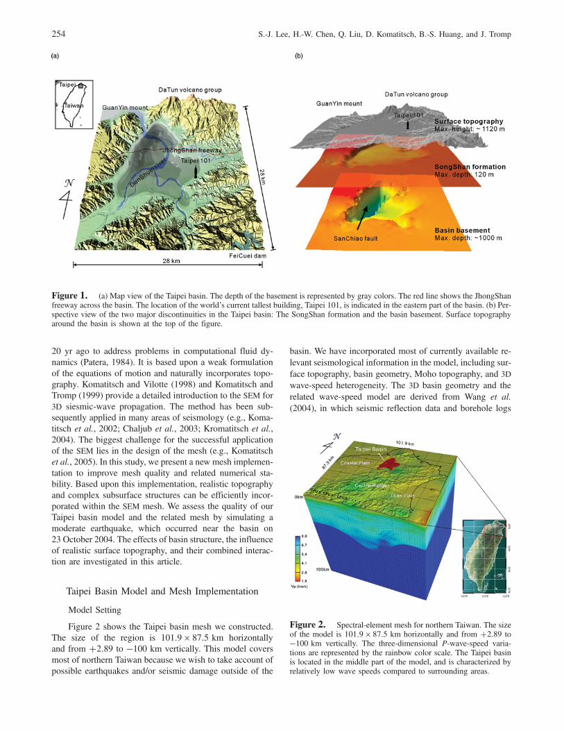
Figure 2 shows the Taipei basin mesh we constructed.The size of the region is 101:9 × 87:5 km horizontallyand from �2:89 to �100 km vertically. This model coversmost of northern Taiwan because we wish to take account ofpossible earthquakes and/or seismic damage outside of the
basin. We have incorporated most of currently available re-levant seismological information in the model, including sur-face topography, basin geometry, Moho topography, and 3Dwave-speed heterogeneity. The 3D basin geometry and therelated wave-speed model are derived from Wang et al.(2004), in which seismic reflection data and borehole logs
Figure 1. (a) Map view of the Taipei basin. The depth of the basement is represented by gray colors. The red line shows the JhongShanfreeway across the basin. The location of the world’s current tallest building, Taipei 101, is indicated in the eastern part of the basin. (b) Per-spective view of the two major discontinuities in the Taipei basin: The SongShan formation and the basin basement. Surface topographyaround the basin is shown at the top of the figure.
Figure 2. Spectral-element mesh for northern Taiwan. The sizeof the model is 101:9 × 87:5 km horizontally and from �2:89 to�100 km vertically. The three-dimensional P-wave-speed varia-tions are represented by the rainbow color scale. The Taipei basinis located in the middle part of the model, and is characterized byrelatively low wave speeds compared to surrounding areas.
254 S.-J. Lee, H.-W. Chen, Q. Liu, D. Komatitsch, B.-S. Huang, and J. Tromp
are combined to characterize the Tertiary basement, the Qua-ternary layers above the basement, and their compressional-and shear-wave speeds. The slowest compressional- andshear-wave speeds in the basin model are 1:5 and0:2 km=sec, respectively. We embed the basin model in aregional tomographic model derived by Kim et al. (2005).The nominal resolution of this background tomographicmodel is 8 km horizontally and 2 km vertically. Theshear-wave-speed outside the basin is computed from thecompressional wave-speed model based upon the assump-tion of a value of 0.25 for Poisson’s ratio. The location ofthe Moho is determined by the 7:8 km=sec isovelocity sur-face in the regional tomographic model. We assign constantwave speeds beneath the Moho (VP � 8:0 km=sec andVS � 4:6 km=sec) to represent the upper mantle. Through-out the entire model, density is defined based upon the em-pirical rule ρ � VP=3� 1280 (McCulloh, 1960; Stidhamet al., 2001) and is constrained to lie between 2000 and3000 kgm�3. Hauksson et al. (1987) determined a shearquality factor of 90 for the Los Angeles basin. Because ofa lack of better attenuation information, we adopt the sameshear quality factor for the Taipei basin and a Q of 500 else-where (i.e., relatively strong attenuation in the sediments andweak attenuation in the bedrock).
Realistic Topography
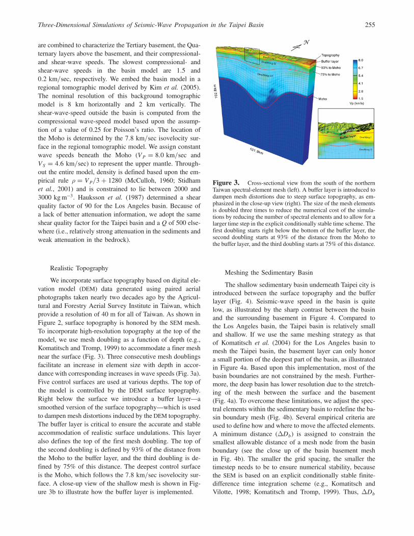
We incorporate surface topography based on digital ele-vation model (DEM) data generated using paired aerialphotographs taken nearly two decades ago by the Agricul-tural and Forestry Aerial Survey Institute in Taiwan, whichprovide a resolution of 40 m for all of Taiwan. As shown inFigure 2, surface topography is honored by the SEM mesh.To incorporate high-resolution topography at the top of themodel, we use mesh doubling as a function of depth (e.g.,Komatitsch and Tromp, 1999) to accommodate a finer meshnear the surface (Fig. 3). Three consecutive mesh doublingsfacilitate an increase in element size with depth in accor-dance with corresponding increases in wave speeds (Fig. 3a).Five control surfaces are used at various depths. The top ofthe model is controlled by the DEM surface topography.Right below the surface we introduce a buffer layer—asmoothed version of the surface topography—which is usedto dampen mesh distortions induced by the DEM topography.The buffer layer is critical to ensure the accurate and stableaccommodation of realistic surface undulations. This layeralso defines the top of the first mesh doubling. The top ofthe second doubling is defined by 93% of the distance fromthe Moho to the buffer layer, and the third doubling is de-fined by 75% of this distance. The deepest control surfaceis the Moho, which follows the 7:8 km=sec isovelocity sur-face. A close-up view of the shallow mesh is shown in Fig-ure 3b to illustrate how the buffer layer is implemented.
Meshing the Sedimentary Basin
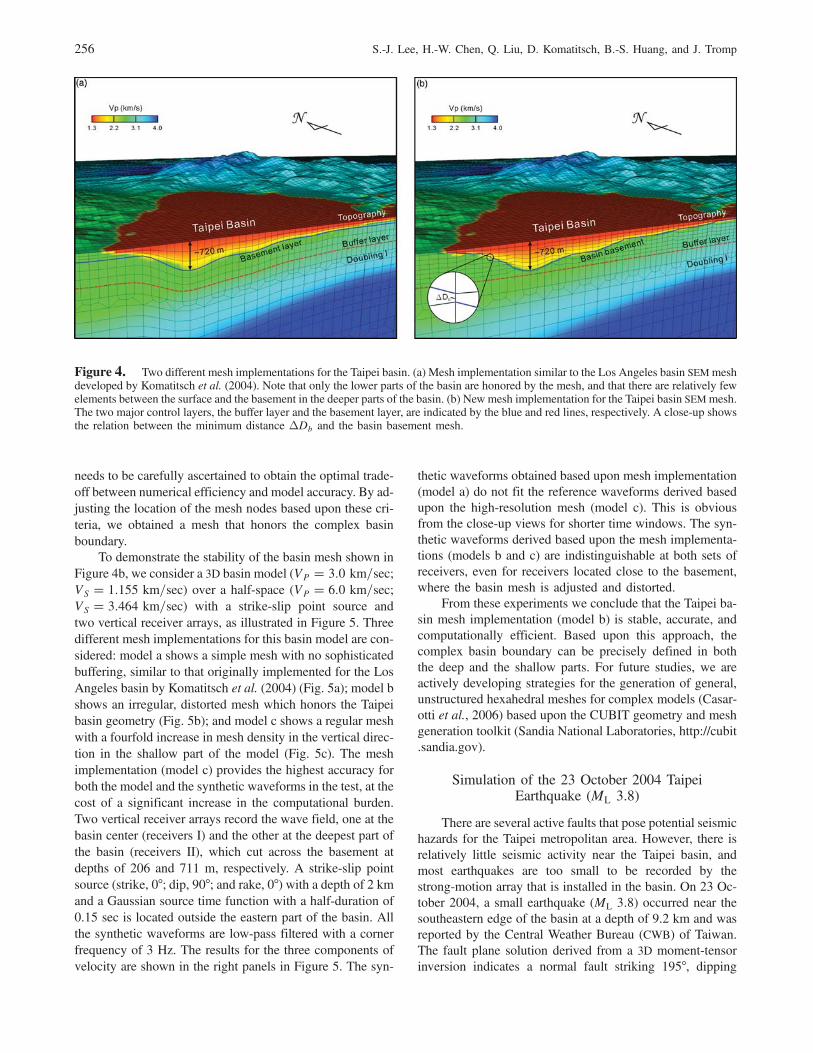
The shallow sedimentary basin underneath Taipei city isintroduced between the surface topography and the bufferlayer (Fig. 4). Seismic-wave speed in the basin is quitelow, as illustrated by the sharp contrast between the basinand the surrounding basement in Figure 4. Compared tothe Los Angeles basin, the Taipei basin is relatively smalland shallow. If we use the same meshing strategy as thatof Komatitsch et al. (2004) for the Los Angeles basin tomesh the Taipei basin, the basement layer can only honora small portion of the deepest part of the basin, as illustratedin Figure 4a. Based upon this implementation, most of thebasin boundaries are not constrained by the mesh. Further-more, the deep basin has lower resolution due to the stretch-ing of the mesh between the surface and the basement(Fig. 4a). To overcome these limitations, we adjust the spec-tral elements within the sedimentary basin to redefine the ba-sin boundary mesh (Fig. 4b). Several empirical criteria areused to define how and where to move the affected elements.A minimum distance (ΔDb) is assigned to constrain thesmallest allowable distance of a mesh node from the basinboundary (see the close up of the basin basement meshin Fig. 4b). The smaller the grid spacing, the smaller thetimestep needs to be to ensure numerical stability, becausethe SEM is based on an explicit conditionally stable finite-difference time integration scheme (e.g., Komatitsch andVilotte, 1998; Komatitsch and Tromp, 1999). Thus, ΔDb
Figure 3. Cross-sectional view from the south of the northernTaiwan spectral-element mesh (left). A buffer layer is introduced todampen mesh distortions due to steep surface topography, as em-phasized in the close-up view (right). The size of the mesh elementsis doubled three times to reduce the numerical cost of the simula-tions by reducing the number of spectral elements and to allow for alarger time step in the explicit conditionally stable time scheme. Thefirst doubling starts right below the bottom of the buffer layer, thesecond doubling starts at 93% of the distance from the Moho tothe buffer layer, and the third doubling starts at 75% of this distance.
Three-Dimensional Simulations of Seismic-Wave Propagation in the Taipei Basin 255
needs to be carefully ascertained to obtain the optimal trade-off between numerical efficiency and model accuracy. By ad-justing the location of the mesh nodes based upon these cri-teria, we obtained a mesh that honors the complex basinboundary.
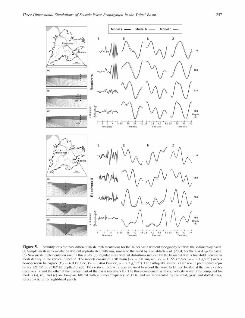
To demonstrate the stability of the basin mesh shown inFigure 4b, we consider a 3D basin model (VP � 3:0 km=sec;VS � 1:155 km=sec) over a half-space (VP � 6:0 km=sec;VS � 3:464 km=sec) with a strike-slip point source andtwo vertical receiver arrays, as illustrated in Figure 5. Threedifferent mesh implementations for this basin model are con-sidered: model a shows a simple mesh with no sophisticatedbuffering, similar to that originally implemented for the LosAngeles basin by Komatitsch et al. (2004) (Fig. 5a); model bshows an irregular, distorted mesh which honors the Taipeibasin geometry (Fig. 5b); and model c shows a regular meshwith a fourfold increase in mesh density in the vertical direc-tion in the shallow part of the model (Fig. 5c). The meshimplementation (model c) provides the highest accuracy forboth the model and the synthetic waveforms in the test, at thecost of a significant increase in the computational burden.Two vertical receiver arrays record the wave field, one at thebasin center (receivers I) and the other at the deepest part ofthe basin (receivers II), which cut across the basement atdepths of 206 and 711 m, respectively. A strike-slip pointsource (strike, 0°; dip, 90°; and rake, 0°) with a depth of 2 kmand a Gaussian source time function with a half-duration of0.15 sec is located outside the eastern part of the basin. Allthe synthetic waveforms are low-pass filtered with a cornerfrequency of 3 Hz. The results for the three components ofvelocity are shown in the right panels in Figure 5. The syn-
thetic waveforms obtained based upon mesh implementation(model a) do not fit the reference waveforms derived basedupon the high-resolution mesh (model c). This is obviousfrom the close-up views for shorter time windows. The syn-thetic waveforms derived based upon the mesh implementa-tions (models b and c) are indistinguishable at both sets ofreceivers, even for receivers located close to the basement,where the basin mesh is adjusted and distorted.
From these experiments we conclude that the Taipei ba-sin mesh implementation (model b) is stable, accurate, andcomputationally efficient. Based upon this approach, thecomplex basin boundary can be precisely defined in boththe deep and the shallow parts. For future studies, we areactively developing strategies for the generation of general,unstructured hexahedral meshes for complex models (Casar-otti et al., 2006) based upon the CUBIT geometry and meshgeneration toolkit (Sandia National Laboratories, http://cubit.sandia.gov).
Simulation of the 23 October 2004 TaipeiEarthquake (ML 3.8)
There are several active faults that pose potential seismichazards for the Taipei metropolitan area. However, there isrelatively little seismic activity near the Taipei basin, andmost earthquakes are too small to be recorded by thestrong-motion array that is installed in the basin. On 23 Oc-tober 2004, a small earthquake (ML 3:8) occurred near thesoutheastern edge of the basin at a depth of 9.2 km and wasreported by the Central Weather Bureau (CWB) of Taiwan.The fault plane solution derived from a 3D moment-tensorinversion indicates a normal fault striking 195°, dipping
Figure 4. Two different mesh implementations for the Taipei basin. (a) Mesh implementation similar to the Los Angeles basin SEMmeshdeveloped by Komatitsch et al. (2004). Note that only the lower parts of the basin are honored by the mesh, and that there are relatively fewelements between the surface and the basement in the deeper parts of the basin. (b) New mesh implementation for the Taipei basin SEMmesh.The two major control layers, the buffer layer and the basement layer, are indicated by the blue and red lines, respectively. A close-up showsthe relation between the minimum distance ΔDb and the basin basement mesh.
256 S.-J. Lee, H.-W. Chen, Q. Liu, D. Komatitsch, B.-S. Huang, and J. Tromp
Figure 5. Stability tests for three different mesh implementations for the Taipei basin without topography but with the sedimentary basin.(a) Simple mesh implementation without sophisticated buffering similar to that used by Komatitsch et al. (2004) for the Los Angeles basin.(b) New mesh implementation used in this study. (c) Regular mesh without distortions induced by the basin but with a four-fold increase inmesh density in the vertical direction. The models consist of a 3D basin (VP � 3:0 km=sec, VS � 1:155 km=sec, ρ � 2:3 g=cm3) over ahomogeneous half-space (VP � 6:0 km=sec, VS � 3:464 km=sec, ρ � 2:7 g=cm3). The earthquake source is a strike-slip point source (epi-center 121.58° E, 25.02° N, depth 2.0 km). Two vertical receiver arrays are used to record the wave field, one located at the basin center(receivers I), and the other at the deepest part of the basin (receivers II). The three-component synthetic velocity waveforms computed formodels (a), (b), and (c) are low-pass filtered with a corner frequency of 3 Hz, and are represented by the solid, gray, and dotted lines,respectively, in the right-hand panels.
Three-Dimensional Simulations of Seismic-Wave Propagation in the Taipei Basin 257
49°, and raking 140° (Lee, Huang, et al., 2006). Because theearthquake is small, the details of the source process can beignored, and we can use a simple point source instead. Thisevent gives us an excellent opportunity to assess our currentvelocity model and the Taipei basin SEM mesh.Because the epicenter of the earthquake is close to the basin,we focus on the Taipei metropolitan area, where most strong-motion instruments were triggered.
We use the SPECFEM3D software package developedby Komatitsch et al. (2004) and decompose the study areainto 324 mesh slices (i.e., 324 processors) for parallel com-puting based upon the message-passing interface (MPI)(Gropp et al., 1996). In each spectral element we use a poly-nomial degree of N � 4, and thus each element con-tains �N � 1�3 � 125 Gauss–Lobatto–Legendre integrationpoints. The average distance between Gauss–Lobatto–Legendre integration points at the surface is 28 m, that is,sufficiently small to resolve the DEM data, and the slowestshear waves within the basin for simulations are accurateup to 1.0 Hz. The simulations are carried out on Caltech’sCITerra Dell cluster (512 dual-processor quad-core nodes).The total number of spectral elements and Gauss–Lobatto–Legendre points in the model is 4,500,000 and 297,000,000,respectively. These simulations require 116 gigabytes ofmemory and the average wall-clock time is 9.5 hr.
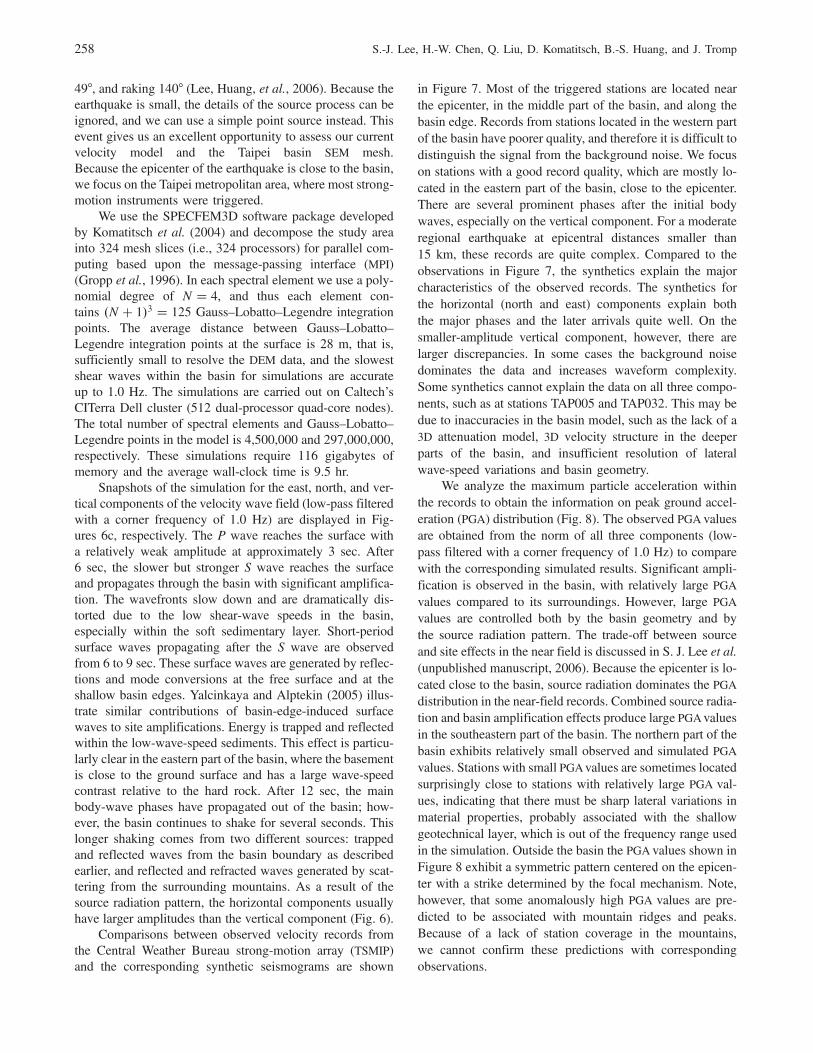
Snapshots of the simulation for the east, north, and ver-tical components of the velocity wave field (low-pass filteredwith a corner frequency of 1.0 Hz) are displayed in Fig-ures 6c, respectively. The P wave reaches the surface witha relatively weak amplitude at approximately 3 sec. After6 sec, the slower but stronger S wave reaches the surfaceand propagates through the basin with significant amplifica-tion. The wavefronts slow down and are dramatically dis-torted due to the low shear-wave speeds in the basin,especially within the soft sedimentary layer. Short-periodsurface waves propagating after the S wave are observedfrom 6 to 9 sec. These surface waves are generated by reflec-tions and mode conversions at the free surface and at theshallow basin edges. Yalcinkaya and Alptekin (2005) illus-trate similar contributions of basin-edge-induced surfacewaves to site amplifications. Energy is trapped and reflectedwithin the low-wave-speed sediments. This effect is particu-larly clear in the eastern part of the basin, where the basementis close to the ground surface and has a large wave-speedcontrast relative to the hard rock. After 12 sec, the mainbody-wave phases have propagated out of the basin; how-ever, the basin continues to shake for several seconds. Thislonger shaking comes from two different sources: trappedand reflected waves from the basin boundary as describedearlier, and reflected and refracted waves generated by scat-tering from the surrounding mountains. As a result of thesource radiation pattern, the horizontal components usuallyhave larger amplitudes than the vertical component (Fig. 6).
Comparisons between observed velocity records fromthe Central Weather Bureau strong-motion array (TSMIP)and the corresponding synthetic seismograms are shown
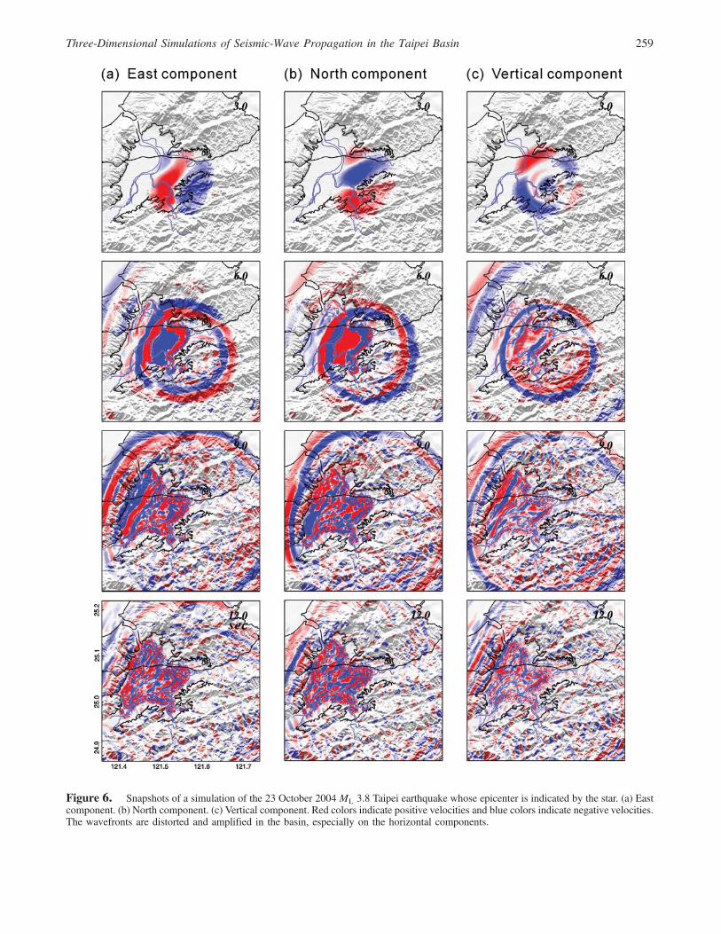
in Figure 7. Most of the triggered stations are located nearthe epicenter, in the middle part of the basin, and along thebasin edge. Records from stations located in the western partof the basin have poorer quality, and therefore it is difficult todistinguish the signal from the background noise. We focuson stations with a good record quality, which are mostly lo-cated in the eastern part of the basin, close to the epicenter.There are several prominent phases after the initial bodywaves, especially on the vertical component. For a moderateregional earthquake at epicentral distances smaller than15 km, these records are quite complex. Compared to theobservations in Figure 7, the synthetics explain the majorcharacteristics of the observed records. The synthetics forthe horizontal (north and east) components explain boththe major phases and the later arrivals quite well. On thesmaller-amplitude vertical component, however, there arelarger discrepancies. In some cases the background noisedominates the data and increases waveform complexity.Some synthetics cannot explain the data on all three compo-nents, such as at stations TAP005 and TAP032. This may bedue to inaccuracies in the basin model, such as the lack of a3D attenuation model, 3D velocity structure in the deeperparts of the basin, and insufficient resolution of lateralwave-speed variations and basin geometry.
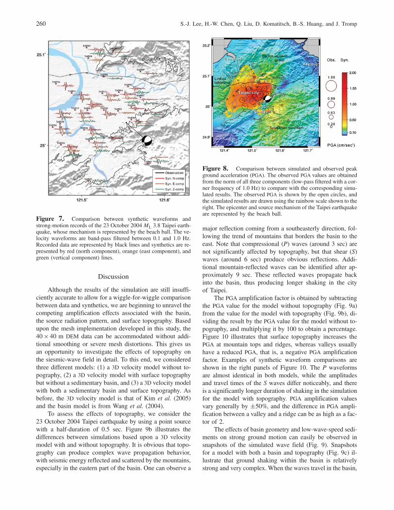
We analyze the maximum particle acceleration withinthe records to obtain the information on peak ground accel-eration (PGA) distribution (Fig. 8). The observed PGA valuesare obtained from the norm of all three components (low-pass filtered with a corner frequency of 1.0 Hz) to comparewith the corresponding simulated results. Significant ampli-fication is observed in the basin, with relatively large PGAvalues compared to its surroundings. However, large PGAvalues are controlled both by the basin geometry and bythe source radiation pattern. The trade-off between sourceand site effects in the near field is discussed in S. J. Lee et al.(unpublished manuscript, 2006). Because the epicenter is lo-cated close to the basin, source radiation dominates the PGAdistribution in the near-field records. Combined source radia-tion and basin amplification effects produce large PGAvaluesin the southeastern part of the basin. The northern part of thebasin exhibits relatively small observed and simulated PGAvalues. Stations with small PGAvalues are sometimes locatedsurprisingly close to stations with relatively large PGA val-ues, indicating that there must be sharp lateral variations inmaterial properties, probably associated with the shallowgeotechnical layer, which is out of the frequency range usedin the simulation. Outside the basin the PGA values shown inFigure 8 exhibit a symmetric pattern centered on the epicen-ter with a strike determined by the focal mechanism. Note,however, that some anomalously high PGA values are pre-dicted to be associated with mountain ridges and peaks.Because of a lack of station coverage in the mountains,we cannot confirm these predictions with correspondingobservations.
258 S.-J. Lee, H.-W. Chen, Q. Liu, D. Komatitsch, B.-S. Huang, and J. Tromp
Figure 6. Snapshots of a simulation of the 23 October 2004 ML 3.8 Taipei earthquake whose epicenter is indicated by the star. (a) Eastcomponent. (b) North component. (c) Vertical component. Red colors indicate positive velocities and blue colors indicate negative velocities.The wavefronts are distorted and amplified in the basin, especially on the horizontal components.
Three-Dimensional Simulations of Seismic-Wave Propagation in the Taipei Basin 259
Discussion
Although the results of the simulation are still insuffi-ciently accurate to allow for a wiggle-for-wiggle comparisonbetween data and synthetics, we are beginning to unravel thecompeting amplification effects associated with the basin,the source radiation pattern, and surface topography. Basedupon the mesh implementation developed in this study, the40 × 40 m DEM data can be accommodated without addi-tional smoothing or severe mesh distortions. This gives usan opportunity to investigate the effects of topography onthe siesmic-wave field in detail. To this end, we consideredthree different models: (1) a 3D velocity model without to-pography, (2) a 3D velocity model with surface topographybut without a sedimentary basin, and (3) a 3D velocity modelwith both a sedimentary basin and surface topography. Asbefore, the 3D velocity model is that of Kim et al. (2005)and the basin model is from Wang et al. (2004).
To assess the effects of topography, we consider the23 October 2004 Taipei earthquake by using a point sourcewith a half-duration of 0.5 sec. Figure 9b illustrates thedifferences between simulations based upon a 3D velocitymodel with and without topography. It is obvious that topo-graphy can produce complex wave propagation behavior,with seismic energy reflected and scattered by the mountains,especially in the eastern part of the basin. One can observe a
major reflection coming from a southeasterly direction, fol-lowing the trend of mountains that borders the basin to theeast. Note that compressional (P) waves (around 3 sec) arenot significantly affected by topography, but that shear (S)waves (around 6 sec) produce obvious reflections. Addi-tional mountain-reflected waves can be identified after ap-proximately 9 sec. These reflected waves propagate backinto the basin, thus producing longer shaking in the cityof Taipei.
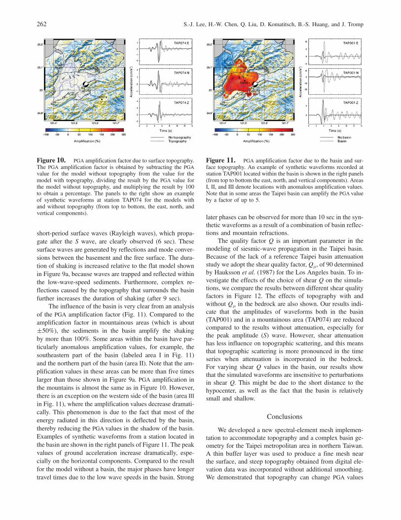
The PGA amplification factor is obtained by subtractingthe PGA value for the model without topography (Fig. 9a)from the value for the model with topography (Fig. 9b), di-viding the result by the PGA value for the model without to-pography, and multiplying it by 100 to obtain a percentage.Figure 10 illustrates that surface topography increases thePGA at mountain tops and ridges, whereas valleys usuallyhave a reduced PGA, that is, a negative PGA amplificationfactor. Examples of synthetic waveform comparisons areshown in the right panels of Figure 10. The P waveformsare almost identical in both models, while the amplitudesand travel times of the S waves differ noticeably, and thereis a significantly longer duration of shaking in the simulationfor the model with topography. PGA amplification valuesvary generally by �50%, and the difference in PGA ampli-fication between a valley and a ridge can be as high as a fac-tor of 2.
The effects of basin geometry and low-wave-speed sedi-ments on strong ground motion can easily be observed insnapshots of the simulated wave field (Fig. 9). Snapshotsfor a model with both a basin and topography (Fig. 9c) il-lustrate that ground shaking within the basin is relativelystrong and very complex. When the waves travel in the basin,
Figure 7. Comparison between synthetic waveforms andstrong-motion records of the 23 October 2004 ML 3.8 Taipei earth-quake, whose mechanism is represented by the beach ball. The ve-locity waveforms are band-pass filtered between 0.1 and 1.0 Hz.Recorded data are represented by black lines and synthetics are re-presented by red (north component), orange (east component), andgreen (vertical component) lines.
Figure 8. Comparison between simulated and observed peakground acceleration (PGA). The observed PGA values are obtainedfrom the norm of all three components (low-pass filtered with a cor-ner frequency of 1.0 Hz) to compare with the corresponding simu-lated results. The observed PGA is shown by the open circles, andthe simulated results are drawn using the rainbow scale shown to theright. The epicenter and source mechanism of the Taipei earthquakeare represented by the beach ball.
260 S.-J. Lee, H.-W. Chen, Q. Liu, D. Komatitsch, B.-S. Huang, and J. Tromp
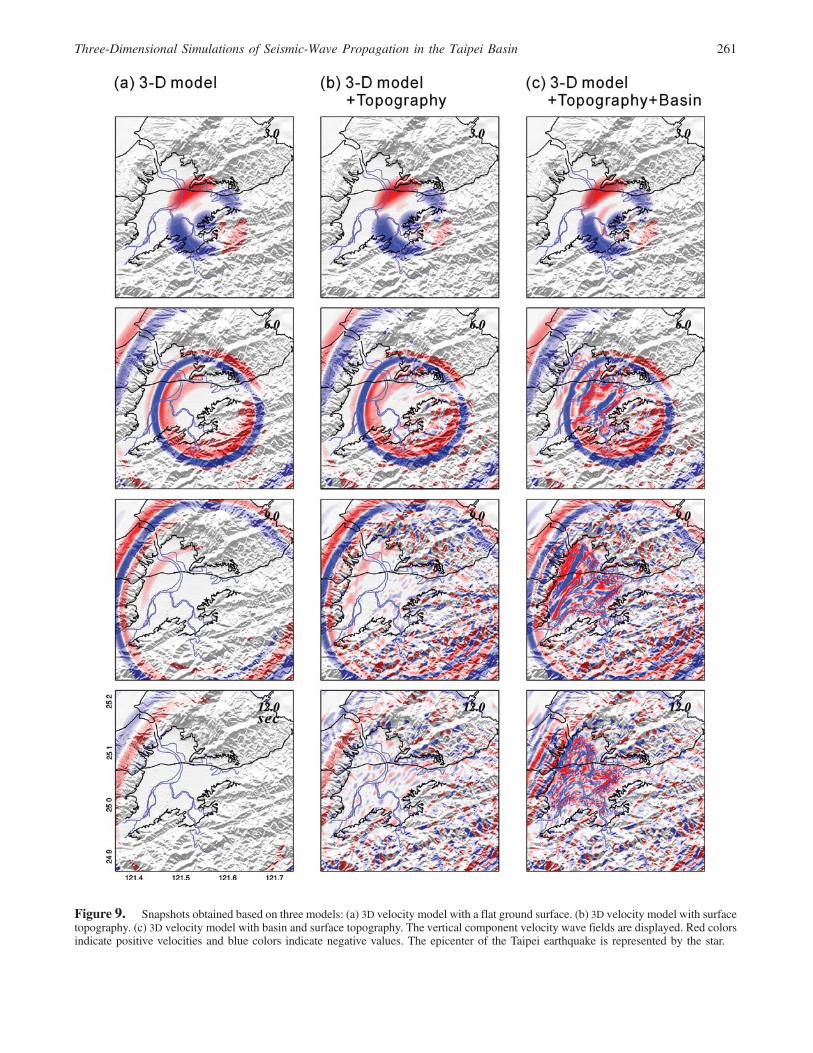
Figure 9. Snapshots obtained based on three models: (a) 3D velocity model with a flat ground surface. (b) 3D velocity model with surfacetopography. (c) 3D velocity model with basin and surface topography. The vertical component velocity wave fields are displayed. Red colorsindicate positive velocities and blue colors indicate negative values. The epicenter of the Taipei earthquake is represented by the star.
Three-Dimensional Simulations of Seismic-Wave Propagation in the Taipei Basin 261
short-period surface waves (Rayleigh waves), which propa-gate after the S wave, are clearly observed (6 sec). Thesesurface waves are generated by reflections and mode conver-sions between the basement and the free surface. The dura-tion of shaking is increased relative to the flat model shownin Figure 9a, because waves are trapped and reflected withinthe low-wave-speed sediments. Furthermore, complex re-flections caused by the topography that surrounds the basinfurther increases the duration of shaking (after 9 sec).
The influence of the basin is very clear from an analysisof the PGA amplification factor (Fig. 11). Compared to theamplification factor in mountainous areas (which is about�50%), the sediments in the basin amplify the shakingby more than 100%. Some areas within the basin have par-ticularly anomalous amplification values, for example, thesoutheastern part of the basin (labeled area I in Fig. 11)and the northern part of the basin (area II). Note that the am-plification values in these areas can be more than five timeslarger than those shown in Figure 9a. PGA amplification inthe mountains is almost the same as in Figure 10. However,there is an exception on the western side of the basin (area IIIin Fig. 11), where the amplification values decrease dramati-cally. This phenomenon is due to the fact that most of theenergy radiated in this direction is deflected by the basin,thereby reducing the PGA values in the shadow of the basin.Examples of synthetic waveforms from a station located inthe basin are shown in the right panels of Figure 11. The peakvalues of ground acceleration increase dramatically, espe-cially on the horizontal components. Compared to the resultfor the model without a basin, the major phases have longertravel times due to the low wave speeds in the basin. Strong
later phases can be observed for more than 10 sec in the syn-thetic waveforms as a result of a combination of basin reflec-tions and mountain refractions.
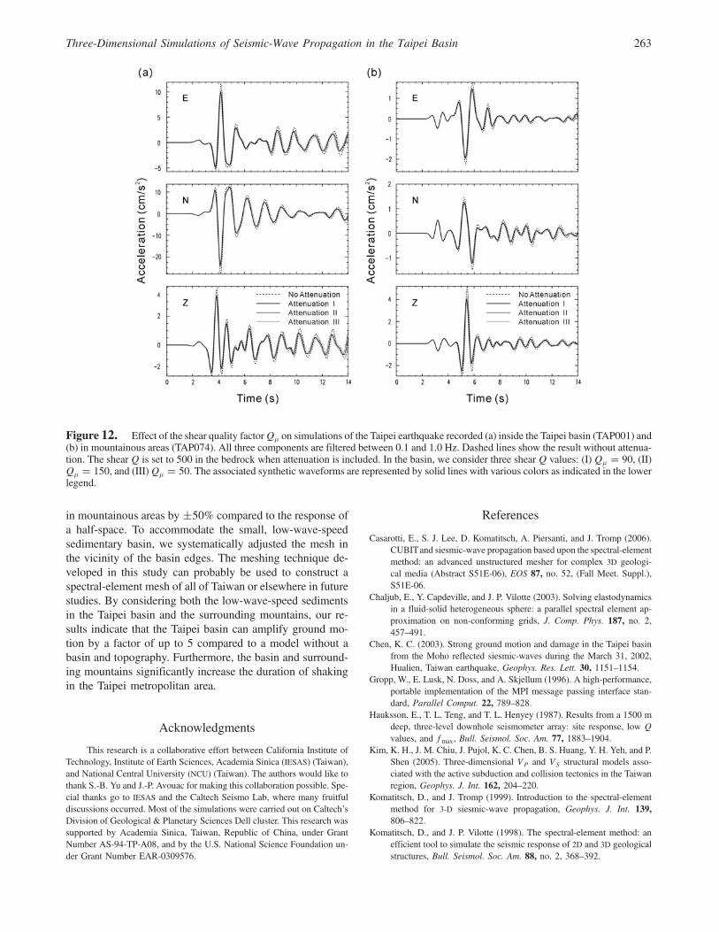
The quality factor Q is an important parameter in themodeling of siesmic-wave propagation in the Taipei basin.Because of the lack of a reference Taipei basin attenuationstudy we adopt the shear quality factor,Qμ, of 90 determinedby Hauksson et al. (1987) for the Los Angeles basin. To in-vestigate the effects of the choice of shear Q on the simula-tions, we compare the results between different shear qualityfactors in Figure 12. The effects of topography with andwithout Qμ in the bedrock are also shown. Our results indi-cate that the amplitudes of waveforms both in the basin(TAP001) and in a mountainous area (TAP074) are reducedcompared to the results without attenuation, especially forthe peak amplitude (S) wave. However, shear attenuationhas less influence on topographic scattering, and this meansthat topographic scattering is more pronounced in the timeseries when attenuation is incorporated in the bedrock.For varying shear Q values in the basin, our results showthat the simulated waveforms are insensitive to perturbationsin shear Q. This might be due to the short distance to thehypocenter, as well as the fact that the basin is relativelysmall and shallow.
Conclusions
We developed a new spectral-element mesh implemen-tation to accommodate topography and a complex basin ge-ometry for the Taipei metropolitan area in northern Taiwan.A thin buffer layer was used to produce a fine mesh nearthe surface, and steep topography obtained from digital ele-vation data was incorporated without additional smoothing.We demonstrated that topography can change PGA values
Figure 10. PGA amplification factor due to surface topography.The PGA amplification factor is obtained by subtracting the PGAvalue for the model without topography from the value for themodel with topography, dividing the result by the PGA value forthe model without topography, and multiplying the result by 100to obtain a percentage. The panels to the right show an exampleof synthetic waveforms at station TAP074 for the models withand without topography (from top to bottom, the east, north, andvertical components).
Figure 11. PGA amplification factor due to the basin and sur-face topography. An example of synthetic waveforms recorded atstation TAP001 located within the basin is shown in the right panels(from top to bottom the east, north, and vertical components). AreasI, II, and III denote locations with anomalous amplification values.Note that in some areas the Taipei basin can amplify the PGA valueby a factor of up to 5.
262 S.-J. Lee, H.-W. Chen, Q. Liu, D. Komatitsch, B.-S. Huang, and J. Tromp
in mountainous areas by�50% compared to the response ofa half-space. To accommodate the small, low-wave-speedsedimentary basin, we systematically adjusted the mesh inthe vicinity of the basin edges. The meshing technique de-veloped in this study can probably be used to construct aspectral-element mesh of all of Taiwan or elsewhere in futurestudies. By considering both the low-wave-speed sedimentsin the Taipei basin and the surrounding mountains, our re-sults indicate that the Taipei basin can amplify ground mo-tion by a factor of up to 5 compared to a model without abasin and topography. Furthermore, the basin and surround-ing mountains significantly increase the duration of shakingin the Taipei metropolitan area.
Acknowledgments
This research is a collaborative effort between California Institute ofTechnology, Institute of Earth Sciences, Academia Sinica (IESAS) (Taiwan),and National Central University (NCU) (Taiwan). The authors would like tothank S.-B. Yu and J.-P. Avouac for making this collaboration possible. Spe-cial thanks go to IESAS and the Caltech Seismo Lab, where many fruitfuldiscussions occurred. Most of the simulations were carried out on Caltech’sDivision of Geological & Planetary Sciences Dell cluster. This research wassupported by Academia Sinica, Taiwan, Republic of China, under GrantNumber AS-94-TP-A08, and by the U.S. National Science Foundation un-der Grant Number EAR-0309576.
References
Casarotti, E., S. J. Lee, D. Komatitsch, A. Piersanti, and J. Tromp (2006).CUBITand siesmic-wave propagation based upon the spectral-elementmethod: an advanced unstructured mesher for complex 3D geologi-cal media (Abstract S51E-06), EOS 87, no. 52, (Fall Meet. Suppl.),S51E-06.
Chaljub, E., Y. Capdeville, and J. P. Vilotte (2003). Solving elastodynamicsin a fluid-solid heterogeneous sphere: a parallel spectral element ap-proximation on non-conforming grids, J. Comp. Phys. 187, no. 2,457–491.
Chen, K. C. (2003). Strong ground motion and damage in the Taipei basinfrom the Moho reflected siesmic-waves during the March 31, 2002,Hualien, Taiwan earthquake, Geophys. Res. Lett. 30, 1151–1154.
Gropp, W., E. Lusk, N. Doss, and A. Skjellum (1996). A high-performance,portable implementation of the MPI message passing interface stan-dard, Parallel Comput. 22, 789–828.
Hauksson, E., T. L. Teng, and T. L. Henyey (1987). Results from a 1500 mdeep, three-level downhole seismometer array: site response, low Q
values, and fmax, Bull. Seismol. Soc. Am. 77, 1883–1904.Kim, K. H., J. M. Chiu, J. Pujol, K. C. Chen, B. S. Huang, Y. H. Yeh, and P.
Shen (2005). Three-dimensional VP and VS structural models asso-ciated with the active subduction and collision tectonics in the Taiwanregion, Geophys. J. Int. 162, 204–220.
Komatitsch, D., and J. Tromp (1999). Introduction to the spectral-elementmethod for 3-D siesmic-wave propagation, Geophys. J. Int. 139,806–822.
Komatitsch, D., and J. P. Vilotte (1998). The spectral-element method: anefficient tool to simulate the seismic response of 2D and 3D geologicalstructures, Bull. Seismol. Soc. Am. 88, no. 2, 368–392.
Figure 12. Effect of the shear quality factorQμ on simulations of the Taipei earthquake recorded (a) inside the Taipei basin (TAP001) and(b) in mountainous areas (TAP074). All three components are filtered between 0.1 and 1.0 Hz. Dashed lines show the result without attenua-tion. The shear Q is set to 500 in the bedrock when attenuation is included. In the basin, we consider three shear Q values: (I) Qμ � 90, (II)Qμ � 150, and (III)Qμ � 50. The associated synthetic waveforms are represented by solid lines with various colors as indicated in the lowerlegend.
Three-Dimensional Simulations of Seismic-Wave Propagation in the Taipei Basin 263
Komatitsch, D., Q. Liu, J. Tromp, P. Süss, C. Stidham, and J. H. Shaw(2004). Simulations of ground motion in the Los Angeles basin basedupon the spectral-element method, Bull. Seismol. Soc. Am. 94,187–206.
Komatitsch, D., J. Ritsema, and J. Tromp (2002). The spectral-elementmethod, Beowulf computing and global seismology, Science 298,1737–1742.
Komatitsch, D., S. Tsuboi, and J. Tromp (2005). The spectral-elementmethod in seismology, in Seismic Earth: Array Analysis of BroadbandSeismograms, Geophysical Monograph Series, A. Levander and G.Nolet (Editors), Vol. 157, American Geophysical Union, Washington,D.C., 205–227.
Lee, S. J., B. S. Huang, and W. T. Liang (2006). Grid-based moment tensorinversion by using spectral-element method 3D Green’s functions(Abstract S11C-0137), EOS 87, no. 36, (West. Pac. Geophys. Meet.Suppl.), S11C-0137.
Lin, C. H. (2005). Seismicity increase after the construction of the world’stallest building: an active blind fault beneath the Taipei 101, Geophys.Res. Lett. 32, no. 22, L22313, doi 10.1029/2005GL024223.
McCulloh, T. H. (1960). Gravity variations and the geology of the LosAngeles basin of California, U.S. Geol. Surv. Profess. Pap. 400-B,320–325.
Olsen, K. B. (2000). Site amplification in the Los Angeles basin from three-dimensional modeling of ground motion, Bull. Seismol. Soc. Am. 90,S77–S94.
Olsen, K. B., R. J. Archuleta, and J. R. Matarese (1995). Three-dimensionalsimulation of a magnitude 7.75 earthquake on the San Andreas fault,Science 270, 1628–1632.
Olsen, K. B., J. C. Pechmann, and G. T. Schuster (1996). An analysis ofsimulated and observed blast records in the Salt Lake basin, Bull.Seismol. Soc. Am. 86, 1061–1076.
Patera, A. T. (1984). A spectral element method for fluid dynamics: laminarflow in a channel expansion, J. Comp. Phys. 54, 468–488.
Robertsson, J. O. A. (1996). A numerical free-surface condition for elastic/viscoelastic finite-difference modeling in the presence of topography,Geophysics 61, 1921–1934.
Stidham, C., M. P. Süss, and J. H. Shaw (2001). 3D density and velocitymodel of the Los Angeles basin, in Geological Society of America2001 Annual Meeting Abstracts, Vol. 33, Geological Society of Amer-ica, Denver, Colorado, 299.
Wald, D. J., and R. W. Graves (1998). The seismic response of the Los An-geles basin, California, Bull. Seismol. Soc. Am. 88, 337–356.
Wang, C. Y., Y. H. Lee, M. L. Ger, and Y. L. Chen (2004). Investigatingsubsurface structures and P- and S-wave velocities in the Taipei basin,TAO 15, 222–250.
Wen, K. L., and H. Y. Peng (1998). Site effect analysis in the Taipei basin:results from TSMIP network data, TAO 9, 691–704.
Wen, K. L., L. Y. Fei, H. Y. Peng, and C. C. Liu (1995). Site effect analysisfrom the records of the Wuku downhole array, TAO 6, 285–29.
Yalcinkaya, E., and O. Alptekin (2005). Contributions of basin-edge-induced surface waves to site effect in the Dinar basin, southwesternTurkey, Pure Appl. Geophys. 162, 931–950.
Institute of Earth SciencesAcademia SinicaNankang, Taipei 115, Taiwan, Republic of [email protected]@earth.sinica.edu.tw
(S.-J.L., B.-S.H.)
Institute of GeophysicsNational Central UniversityJung-Li 320, Taiwan, Republic of [email protected]
(H.-W.C.)
Seismological LaboratoryCalifornia Institute of TechnologyPasadena, [email protected]@gps.caltech.edu
(Q.L., J.T.)
Department of Geophysical Modeling and Imaging in GeosciencesCNRS UMR 5212 and INRIA Magique 3DUniversity of PauFrance
(D.K.)
Manuscript received 23 February 2007
264 S.-J. Lee, H.-W. Chen, Q. Liu, D. Komatitsch, B.-S. Huang, and J. Tromp