Draft THREE-DIMENSIONAL TRAJECTORY TRACKING CONTROL OF AN UNDERACTUATED AUV BASED ON ROBUST ADAPTIVE ALGORITHM Journal: Transactions of the Canadian Society for Mechanical Engineering Manuscript ID TCSME-2018-0123.R1 Manuscript Type: Article Date Submitted by the Author: 29-Jul-2018 Complete List of Authors: Jiang, Yunbiao; Dalian Maritime University, School of marine Electrical Engineering Guo, Chen; Dalian Maritime University Yu, Haomiao ; Dalian Maritime University, School of Marine Electrical Engineering Keywords: AUV, Three-dimensional trajectory tracking, Virtual velocity control, Non- singular terminal sliding mode control (NTSMC) Is the invited manuscript for consideration in a Special Issue? : Not applicable (regular submission) https://mc06.manuscriptcentral.com/tcsme-pubs Transactions of the Canadian Society for Mechanical Engineering
Transcript
Draft
THREE-DIMENSIONAL TRAJECTORY TRACKING CONTROL OF AN UNDERACTUATED AUV BASED ON ROBUST ADAPTIVE
ALGORITHM
Journal: Transactions of the Canadian Society for Mechanical Engineering
Manuscript ID TCSME-2018-0123.R1
Manuscript Type: Article
Date Submitted by the Author: 29-Jul-2018
Complete List of Authors: Jiang, Yunbiao; Dalian Maritime University, School of marine Electrical Engineering Guo, Chen; Dalian Maritime UniversityYu, Haomiao ; Dalian Maritime University, School of Marine Electrical Engineering
2. Ghen Guo*: Corresponding author, Professor, School of Marine Electrical Engineering, Dalian Maritime University. Email: [email protected].
3. Hoamiao Yu: Doctor, School of Marine Electrical Engineering, Dalian Maritime University. Email: [email protected].
.
Page 1 of 26
https://mc06.manuscriptcentral.com/tcsme-pubs
Transactions of the Canadian Society for Mechanical Engineering
Draft
ABSTRACT: This paper investigates the problem of three-dimensional trajectory tracking control for an underactuated autonomous underwater vehicle (AUV) in the presence of uncertain disturbances. The concept of virtual velocity control is adopted and the desired velocities are designed by using the backstepping method. Then, the trajectory tracking problem is transformed into the stabilization problem of the virtual velocity errors. The dynamic control laws are developed based on the non-singular terminal sliding mode control (NTSMC) to stabilize the virtual velocity errors, and adaptive laws are introduced to deal with the parameters perturbation and current disturbances. The stability of the closed-loop control system is analyzed based on the Lyapunov stability theory, and two sets of typical simulations are carried out to verify that the effectiveness and robustness of the trajectory tracking control algorithm designed in this paper under uncertain disturbances. Keywords: underactuated AUV; three-dimensional trajectory tracking; virtual velocity control; NTSMC; robustness.
Page 2 of 26
https://mc06.manuscriptcentral.com/tcsme-pubs
Transactions of the Canadian Society for Mechanical Engineering
Draft
1. INTRODUCTION
1
The motion control of underactuated autonomous underwater vehicles (AUVs) has always been a great concern, and a lot of outstanding achievements have been witnessed over past decades. Precise trajectory tracking control of AUVs is an important technical prerequisite for some specific tasks, such as oceanographic mapping, marine hydrographic survey and military applications (Yan et al., 2015). Since most AUVs are underactuated configuration and belong to the second order nonholonomic system, so it does not satisfy the necessary condition of the Brockett theorem (Fakhreddin et al., 2014). Taking into account the variability of the marine environment, the parameters perturbation and ocean current disturbances should be considered in the controller design. Compared with path following, the trajectory tracking also has time constraint. Considering the strong nonlinearity of AUV’s mathematical model and uncertain disturbance, it is necessary to develop a robust controller for the trajectory tracking control for underactuated AUVs.
With the development of nonlinear control theory, many intelligent control algorithms have been adopted for the trajectory tracking control of underactuated AUVs, such as sliding mode control, neural network control, fuzzy control, internal model control, robust adaptive control and various combined control of these algorithms (Luis et al., 2016; Karkoub et al., 2017; Shojaei, 2017; Cui et al., 2017; Yu et al., 2012; Cui et al., 2016; Zakeri et al., 2016; Liu et al., 2016; Bouzid et al., 2016; Zhu et al., 2018). In practice, most AUVs are underactuated configuration with asymmetric saturation actuators. The sway and heave motion of an underactuated AUV can only be controlled by the coupling torque, while the control inputs are also limited. For this issue, many specific control strategies are derived (Do, 2015; Zheng et al., 2015; Casau et al., 2015; Park, 2017; Huang et al., 2015). Taking into account the internal parameters perturbation and ocean current disturbances, the adaptive strategy is widely used to combine with other intelligent control algorithms. An adaptive trajectory tracking controller based on the desired state-dependent regressor matrix is proposed in Sahu and Subudhi (2014), which can effectively handle the problem of hydrodynamic parametric uncertainties. The following year, a kind of adaptive tracking control strategy that can track both straight line trajectory and curve trajectory with high accuracy is proposed in Dong et al. (2015), and the well-known Persistent Exciting (PE) condition of yaw velocity is completely liberalized in that study. In Chen et al.(2016) and Qiao et al. (2017), two kinds of adaptive controllers are designed which both have excellent trajectory tracking performance in the presence of model parameter uncertainties. A time-varying trajectory tracking control law based on the direct estimation of dynamic variables is proposed in Rezazadegan et al. (2015), which can effectively overcome the unknown internal and external disturbances.
The sliding mode control (SMC) is a special discontinuous control method, which can dynamically switch its “control structure” according to the current states of the system. It is due to the robustness of sliding mode control that it has been widely used in the control of uncertain systems. An adaptive second-order fast nonsingular terminal sliding mode control scheme for the trajectory tracking of AUVs is proposed in Qiao et al. (2018), which has a faster exponential convergence rate and does not need to know the upper bound of the system uncertainty. In Liang et al. (2016), the tracking controller was designed by combining sliding mode control with fuzzy logic theory and simulations and outfield tests show that the controller has excellent adaptability and robustness in the presence of parameter uncertainties and external disturbances. In Elmokadem et al. (2016), three trajectory tracking controllers are designed based on the terminal sliding mode for an underactuated AUV. They not only have excellent tracking performance, but also have advantages in convergence rate, stability and anti-interference ability respectively.
There are still many achievements on trajectory tracking control for AUVs, but some of them have their own drawbacks and limitations. For example, some control algorithms can only realize two-dimensional trajectory tracking, while some can only achieve linear trajectory tracking (Bouzid et al., 2016; Huang et al., 2015; Repoulias and Papadopoulos, 2007; Aguiar and Hespanha, 2007; Xu et al.,
Page 3 of 26
https://mc06.manuscriptcentral.com/tcsme-pubs
Transactions of the Canadian Society for Mechanical Engineering
Draft
2015; Dong et al., 2015). Every coin has two sides, quite a lot advanced control algorithms are very complex and have higher demands on actuators.
In this paper, an adaptive tracking control algorithm based on the backstepping method and NTSMC is proposed which can realize the three-dimensional trajectory tracking of an underactuated AUV under uncertain disturbances. This control strategy avoids the chattering problem and reduces the requirements for AUV actuators and increases the practical feasibility. The rest of this paper is organized as follows. Section 2 presents a generic model of underactuated AUVs and formulates the transformation of trajectory tracking problem. Section 3 describes the design process of proposed control algorithm in detail and stability analysis was performed based on Lyapunov theorem. The performance of the control algorithm is verified by numerical simulation, and the results are given in Section 4. In addition, a brief summary of this work is made in Section 5.
2. PROBLEM FORMATION
2.1. AUV Modeling Taking a standard approach, modeling an AUV can be divided into two parts which are kinematics and
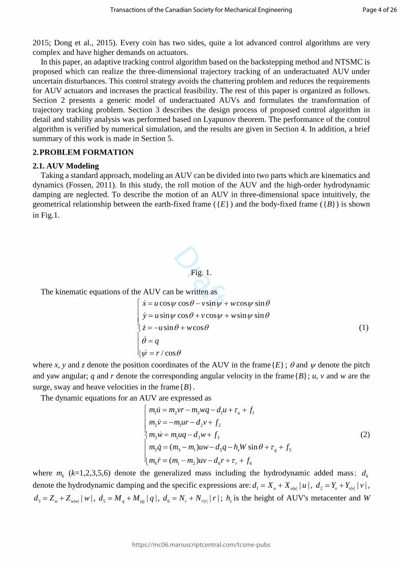
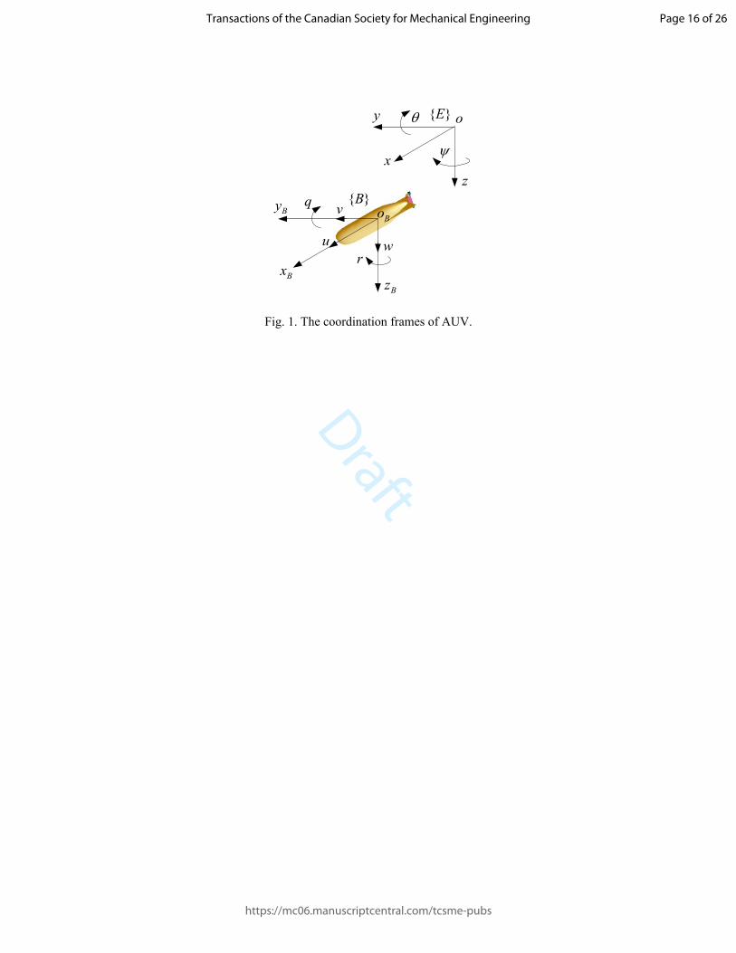
dynamics (Fossen, 2011). In this study, the roll motion of the AUV and the high-order hydrodynamic damping are neglected. To describe the motion of an AUV in three-dimensional space intuitively, the geometrical relationship between the earth-fixed frame ({ }E ) and the body-fixed frame ({ }B ) is shown in Fig.1.
Fig. 1.
The kinematic equations of the AUV can be written as
cos cos sin cos sinsin cos cos sin sinsin cos
/ cos
x u v wy u v wz u w
qr
y q y y qy q y y qq q
qy q
= − + = + + = − + = =
(1)
where x, y and z denote the position coordinates of the AUV in the frame{ }E ; q and y denote the pitch and yaw angular; q and r denote the corresponding angular velocity in the frame{ }B ; u, v and w are the surge, sway and heave velocities in the frame{ }B .
The dynamic equations for an AUV are expressed as
1 2 3 1 1
2 1 2 2
3 1 3 3
5 3 1 5 5
6 1 2 6 6
( ) sin
( )
u
z q
r
m u m vr m wq d u fm v m ur d v fm w m uq d w fm q m m uw d q h W fm r m m uv d r f
τ
q τ
τ
= − − + +
= − − + = − + = − − − + + = − − + +
(2)
where km (k=1,2,3,5,6) denote the generalized mass including the hydrodynamic added mass; kd denote the hydrodynamic damping and the specific expressions are: 1 | | | |u u ud X X u= + , 2 | | | |v v vd Y Y v= + ,
3 | | | |w w wd Z Z w= + , 5 | | | |q qd M M q= + , 6 | | | |r r rd N N r= + ; zh is the height of AUV's metacenter and W
Page 4 of 26
https://mc06.manuscriptcentral.com/tcsme-pubs
Transactions of the Canadian Society for Mechanical Engineering
Draft
is the buoyancy suffered by the AUV; The available control inputs are the surge force uτ , the pitch torque
qτ and the yaw torque rτ . kf denote the ocean current disturbing torque. Obviously, the AUV described by Eq. (1) and Eq. (2) is underactuated and the underactuated AUV
have unintegrable acceleration constraints and belongs to the nonholonomic system, but still controllable in finite-time (Yan et al., 2015; Zhang and Wu, 2015).
lemma1. There is no direct control force for the sway and heave motion of an underactuated AUV, but the velocities v and w are still bounded.
Proof. Choose the Lyapunov function candidate as follows: 21
2vV v= (3)
By using Eq. (3), the derivative of vV with respect to time can express as
1 2 2 22
2 1 2
2
( ) /
( )vV vv v m ur d v f m
d v m ur f vm
= = − − +
− − +=
(4)
Since 2 0d > and 2 0m > , 0vV < when 1 2 2( ) /v m ur f d> + . In addition, 0vV < indicates v is decreasing. Therefore, the proof of v is bounded is complete.
In the same way, w is bounded can also be proved and not tired in words here.
2.1 Transformation of Tracking Problem In this section, the trajectory tracking error equations are established and the tracking problem is
transformed into the error stabilization problem. Considering the motion of the underactuated AUV in three-dimensional space, we can define the
position tracking errors as follows: [ , , ] [ , , ]T T
e e e d d dx y z x x y y z z= − − − (5)
where ( , , )d d dx y z is the position coordinates of the desired time-varying trajectory in the earth-fixed frame.
Combined with Eq. (2), and the time derivatives of the tracking errors in Eq. (4) are as follows: e d
e p d
e d
x xuy v y
wz z
= −
J (6)
where cos cos sin cos sinsin cos cos sin sin
sin 0 cosp
y q y y qy q y y q
y q
− = −
J .
At the same time, the velocity errors are defined as [ ] [ ], , , ,T T
e e e d d du v w u u v v w w= − − − (7)
where du , dv and dw are the desired surge, sway and heave velocities respectively, which are designed latter. Taking the time derivatives of Eq. (7) and considering Eq. (2), yield
2 3 1 1
1 2 2
1 3 3
( ) /( ) /( ) /
e u d
e d
e d
u m vr m wq d u m uv m ur d v m vw m uq d w m w
τ= − − + − = − − − = − −
(8)
Therefore, the trajectory tracking problem has been transformed into the velocity errors stabilization.
Page 5 of 26
https://mc06.manuscriptcentral.com/tcsme-pubs
Transactions of the Canadian Society for Mechanical Engineering
Draft
3. CONTROL LAW DESIGN
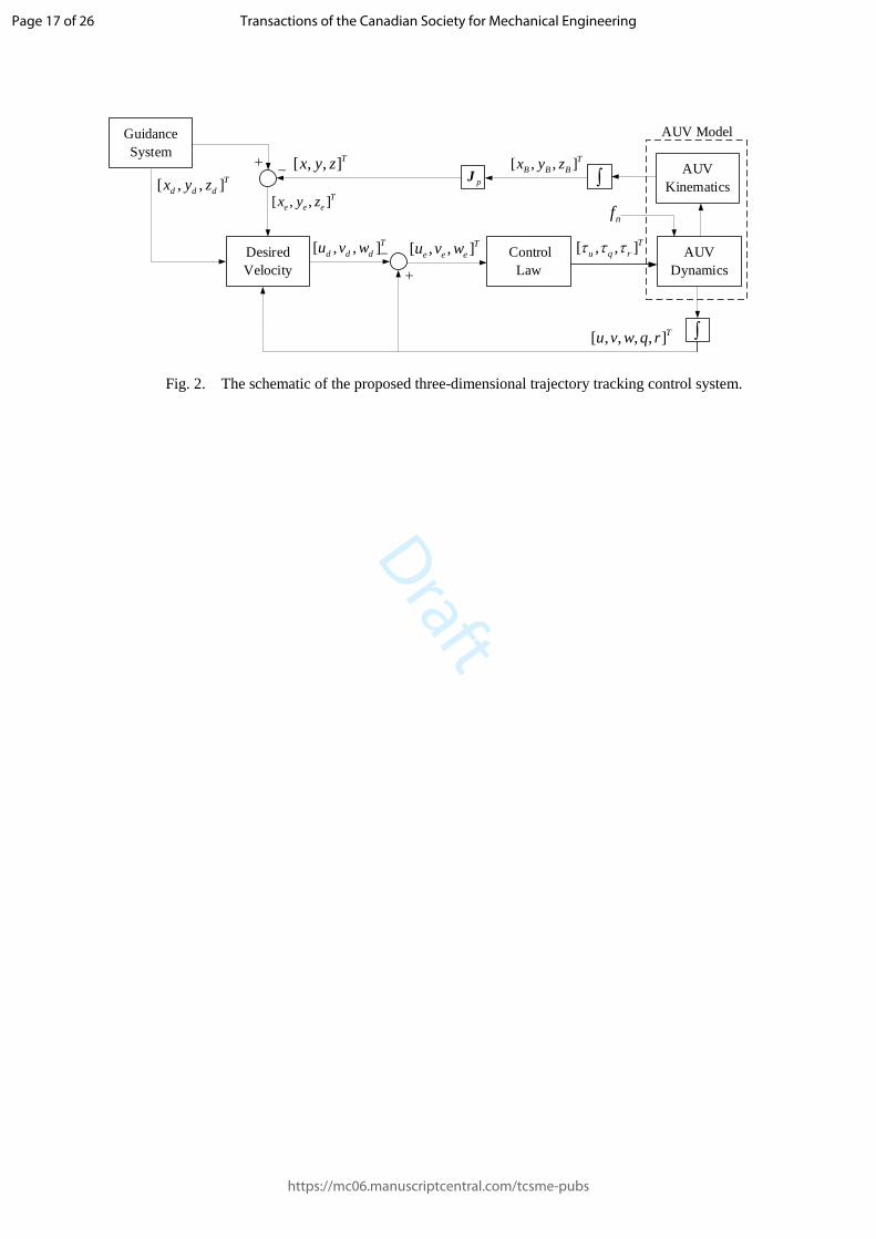
The procedure of designing the trajectory tracking control law is divided into two parts: the design of desired velocity variables and the derivation of the dynamics control law. The control law is developed by using the non-singular terminal sliding mode control and backstepping method. Meanwhile, the stabili ty is guaranteed by Lyapunov theorem.
Fig. 2.
3.1 Desired Velocities Design In this part, the desired surge, sway and heave velocities are designed to ensure the AUV’s position
tracking errors convergent to zero. The equation derived from Eq. (1) is as follows:
= Tp
u xv yw z
J (9)
The desired velocities are designed as follows: tanh( / )
= tanh( / )
tanh( / )
d d x x x eT
d p d y y y e
d d z z z e
u x xv y yw z z
a β aa β a
a β a
−
−
−
+ + +
J
(10)
where | | 1 sin sinTp y q= +J and ( / 2, / 2)q π π∈ − , so T
pJ is non-singular; xa , ya and za are non-zero; xβ , yβ and zβ are positive constants.
By substituting Eq. (9) and Eq. (10) into Eq. (7) leads to the follows: tanh( / )tanh( / )
tanh( / )
e e x x x eT
e p e y y y e
e e z z z e
u x xv y yw z z
a β aa β a
a β a
−
−
−
− = − −
J
(11)
According to Eq. (10), it is clear that the convergence of the velocity errors eu , ev and ew can guarantee the following equations,
tanh( / )tanh( / )
tanh( / )
e x x x e
e y y y e
e z z z e
x xy yz z
a β aa β a
a β a
−
−
−
= = =
. (12)
Consider the Lyapunov function candidate as 2 2 21 1 1=
2 2 2k e e eV x y z+ + (13)
and taking the time derivative of kV along Eq. (13) yields
tanh( / ) tanh( / ) tanh( / )k e e e e e e
x e x x e y e y y e z e z z e
V x x y y z zx x y y z za β a a β a a β a
= + += − − −
(14)
Since xa , ya , za , xβ , yβ and zβ are positive and considering the nature of the odd function tanh( )⋅ , it
can be ensured that 0kV < when ( , , ) (0,0,0)e e ex y z ≠ . At the same time, 0kV < also means that ( , , )e e ex y z will asymptotically convergent to zero in finite time.
Page 6 of 26
https://mc06.manuscriptcentral.com/tcsme-pubs
Transactions of the Canadian Society for Mechanical Engineering
Draft
Thus, it has been proved that the convergence of the velocity errors can guaranteed the position tracking errors are asymptotically convergent to zero.
3.2 Control Law Design Based on NTSMC In this part, the dynamic control laws are developed by adopting the non-singular terminal sliding
mode control (NTSMC), which can forces the velocity errors to converge to zero.
Remark1. All the states of the AUV are measurable and the delay of the feedback system can be ignored.
3.2.1 The control law for surge force uτ
The global non-singular sliding surface in term of the surge velocity error is chosen as 1
1 10( ) + (0)
t be e eS u d u uτ τ λ= −∫ (15)
where 1 0λ > , 1b is odd integer and satisfies 1 1b > . By taking the time derivative of 1S along the error dynamic in Eq.(11), we can obtain
( )
1
1
11 1 1
11 1 2 3 1 1 1( ) /
be e e
be u d e
S u b u u
u b m vr m wq d u f m u u
λ
λ τ
−
−
= +
= + − − + + −
(16)
Then, the Lyapunov function candidate is chosen as 2 2
1 1 1 11 12 2
V S fξ= + (17)
where 1 1 1̂f f f= − , 1̂f is the adaptive estimated value of 1f which will be designed later. In order to ensure the derivative 1V to be negative, the control law for surge force uτ is design as
follows: 121
2 3 1 1 1 1 1 11 1
ˆ sgn( )bu d e
mm vr m wq d u f m u u m Sb
τ eλ
−= − + + − + − − (18)
where 1e is positive constant. According to relevant literatures and preliminary simulations, we can know that the sign function
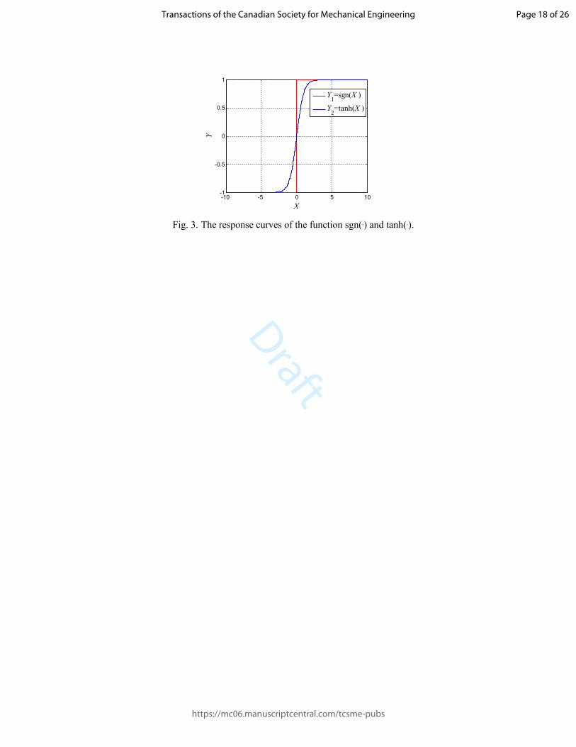
sgn( )⋅ could cause the chattering problem which is common in the traditional sliding mode control. Therefore, this paper uses the hyperbolic tangent function tanh( )⋅ to replace sgn( )⋅ and their response curves are shown in Fig. 3.
Fig. 3.
Obviously, the function tanh( )⋅ is relatively smooth, which is conducive to the stability of the control system. Then, the control law uτ can be rewritten as
1212 3 1 1 1 1 1 1
1 1
ˆ tanh( )bu d e
mm vr m wq d u f m u u m Sb
τ eλ
−= − + + − + − − (19)
Taking the time derivative of 1V and substituting Eq. (19) into it, then
(( ) )1
1 1 1 1 1 1
11 1 1 2 3 1 1 1
1 1 1 1 1 1 1 1 1 1 1 1
11 1 1 1 1 1 1 1 1 1 1 1 1
( ) /
ˆsgn( ) / ( )
ˆ| | ( / )
be u d e
V S S f f
S u b m vr m wq d u f m u u
S S b f S m f f f
S f f f f b S m
ξ
λ τ
e λ ξ
e ξ ξ λ ξ
−
−
= +
= + − − + + −
= − + + −
≤ − + − −
(20)
Page 7 of 26
https://mc06.manuscriptcentral.com/tcsme-pubs
Transactions of the Canadian Society for Mechanical Engineering
Draft
The design of the adaptive law and the specific stability analysis of the control system are performed later.
3.2.2 The control laws for pitch torque qτ and yaw torque rτ
Similar to the procedure progress,the non-singular sliding surfaces in terms of the heave and sway velocity errors are chosen as:
22 2 (0)b
e e eS w w wλ= + − (21) 3
3 3 (0)be e eS v v vλ= + − (22)
where 0( 2,3)i iλ > = , ib is odd integers and satisfies 1ib > . The time derivatives of 2S and 3S along the error dynamic can be calculated as follows:
( ( )
( ) )
2
2
12 2 2
1 22 2 1 3 3
1 3 3 1 5 5 5
( ) / sec
( / ) ( ) sin /
be e e
b ze e z e
z
d z q
e
S w b w w
w b w m uq d w m z h z
m u m w m m uw d q h W f m
βa
λ
λ β
q τ
−
−
= +
= + − −
− + − − − + +
−
(23)
( ( )
( ) )
3
3
13 3 3
1 23 3 1 2 2
1 2 1 2 6 6 6
( ) / sec
( / ) ( ) /
be e e
ybe e y e
y
d r
e
S v b v v
v b v m ur d v m y h y
m u m u m m uv d r f m
β
a
λ
λ β
τ
−
−
= +
= + − − −
− + − − + +
−
(24)
Hence, let the Lyapunov function candidate be chosen as
2 2 2 22 2 3 2 5 3 6
1 1 1 12 2 2 2
V S S f fξ ξ= + + + (25)
where 5 5 5̂f f f= − and 6 6 6̂.f f f= − 5̂f and 6̂f are the adaptive estimated value of 5f and 6f which will be designed later.
Taking the derivative of 2V with respect to time and to ensure the derivative 2V to be negative, the sway and heave motion control law qτ and rτ is chosen as follows:
(
)2
51 3 5 5 1 3 3
1 32
22 2
2 2
ˆ( ) sin + ( ) /( / )
sec tanh( )( )
q zd
bez
z e ez
mm m uw d q h W f m uq d w mm u m w
wz h z Sb
βa
τ q
β eλ
−
= − + + − − ++
+ − − −
(26)
(
)3
62 1 6 6 1 2 2
1 22
2e 3 3
3 3
ˆ( ) + ( ) /( / )
sec tanh( )( )
rd
by e
y ey
mm m uv d r f m ur d v mm u m u
vy h y Sb
β
a
τ
β eλ
−
= − + − ++
+ − − −
(27)
Taking the time derivative of V2 and substituting Eq. (25) and Eq. (26) into it, we can obtain
2 2 2 3 3 2 5 5 2 6 6
2 2 3 3 2 5 5 3 6 6
1 12 5 5 2 2 2 2 5 3 6 6 3 3 3 3 6
| | | |
ˆ ˆ( / ) ( / )
V S S S S f f f f
S S f f f f
f f b S m f f b S m
ξ ξ
e e ξ ξ
ξ λ ξ ξ λ ξ− −
= + + +
≤ − − + +
− − − −
(28)
Page 8 of 26
https://mc06.manuscriptcentral.com/tcsme-pubs
Transactions of the Canadian Society for Mechanical Engineering
Draft
Then the adaptive estimated value of 1f , 5f and 6f will be introduced to ensure that 1V and 2V are negative.
3.3 Adaptive Law In order to stabilize the velocity errors and ensure the stability of the dynamic control system under
bounded disturbance, the adaptive laws are designed as follows: 1
1 1 1 1 1 1
15 2 2 2 2 5
16 3 3 3 3 6
ˆ = /
ˆ = /
ˆ = /
f b S m
f b S m
f b S m
λ ξ
λ ξ
λ ξ
−
−
−
(29)
Lemma2. With the adaptive tracking control law, the surge, sway and heave velocities will converge to their desired value in finite time.
Proof. For the dynamic control system, we choose the Lyapunov function candidate as 2 2 2 2 2 2
1 2 1 2 3 1 1 2 5 3 61 1 1 1 1 12 2 2 2 2 2dV V V S S S f f fξ ξ ξ= + = + + + + + (30)
Taking the time derivative of dV , and substituting Eq. (19), Eq. (26) and Eq. (27) into it, we can have
1 1 2 2 3 3 1 1 1 2 5 5 3 6 6| | | | | |dV S S S f f f f f fe e e ξ ξ ξ≤ − − − + + + (31)
Remark2. The underwater vehicles operate in the deep-sea environment, and the current disturbances are generally assumed to be constant or slow time-varying.
The two cases of disturbance are respectively discussed as follows: 1) The disturbances 1f , 5f and 6f are constant and 1 5 6 0f f f= = = , then the Eq. (31) can be rewritten
as
1 1 2 2 3 3 1 1 1 2 5 5 3 6 6
1 1 2 2 3 3
| | | | | || | | | | | 0
dV S S S f f f f f fS S S
e e e ξ ξ ξe e e
≤ − − − + + +≤ − − − ≤
(32)
2) The disturbance 1f , 5f and 6f are slow time-varying, so 1 0f ≈ , 5 0f ≈ , 6 0f ≈ . It can be seen from Eq. (31) that dV can be guaranteed negative by adjusting the value of 1e , 2e , 3e , 1ξ , 2ξ , 3ξ , i.e. we can guarantee that
1 1 2 2 3 3 1 1 1 2 5 5 3 6 6| | | | | | 0dV S S S f f f f f fe e e ξ ξ ξ≤ − − − + + + ≤ (33)
Thus, it has been proved that the adaptive control laws can drive the velocities to converge to their desired value. Furthermore, combined with the conclusion of the section 3.1, we can conclude that the position tracking errors ex , ey and ez can convergent to zero under the control algorithm and the whole system is globally asymptotically stable. That is the control law proposed in this paper can realize the three dimensional trajectory tracking of underactuated AUVs.
4. NUMERICAL SIMULATIONS
In this section, a series of numerical simulations are carried out to demonstrate the effectiveness and robustness of the trajectory tracking control algorithm proposed in this paper. The physical parameters of the AUV in the simulation come from Zhou et al. (2017), and the simulation results are also compared with Zhou et al. (2017) correspondingly. The relevant specific parameters are as follows:
| | =100kg mr rN ⋅ , 0.2mzh = , 1814NW = . Considering the actual situation, the above
Page 9 of 26
https://mc06.manuscriptcentral.com/tcsme-pubs
Transactions of the Canadian Society for Mechanical Engineering
Draft
parameters have 10%± perturbation set in the simulation. At the same time, the slow time-varying ocean current disturbance is set as:
1 2 3 5 6[ , , , , ] [20 10sin(0.02 ),0,0,5sin(0.01 ),5sin(0.05 ) 5cos(0.02 )] NT Tf f f f f t t t t= = + +f . To illustrate the trajectory tracking performance of the proposed control algorithm well, two sets of
simulation case were set up. The two simulation cases use the same control parameters which are selected as:
Case 1: Spiral trajectory tracking The desired spiral trajectory is described as:
100sin(0.01 ) m100cos(0.01 ) m0.1 m
R
R
R
x ty tz t
= = =
(34)
The initial states of the AUV are set as [ (0), (0), (0), (0), (0)] [0(m), 95(m),10(m), 0(rad), 0(rad)]T Tx y z q y = ;
[ (0), (0), (0)] [0(m / s), 0(m / s), 0(m / s)]T Tu v w = ; [ (0), (0)] [0(rad / s), 0(rad / s)]T Tq r = , and the simulation results and analysis are as blew.
Fig. 4.
(a). (b). Fig. 5.
(a). (b). Fig. 6.
(a). (b). Fig. 7.
Page 10 of 26
https://mc06.manuscriptcentral.com/tcsme-pubs
Transactions of the Canadian Society for Mechanical Engineering
Draft
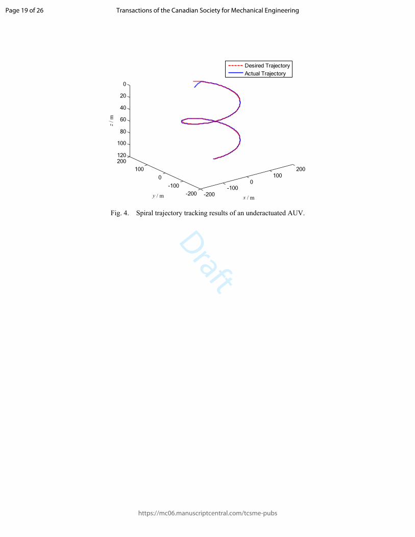
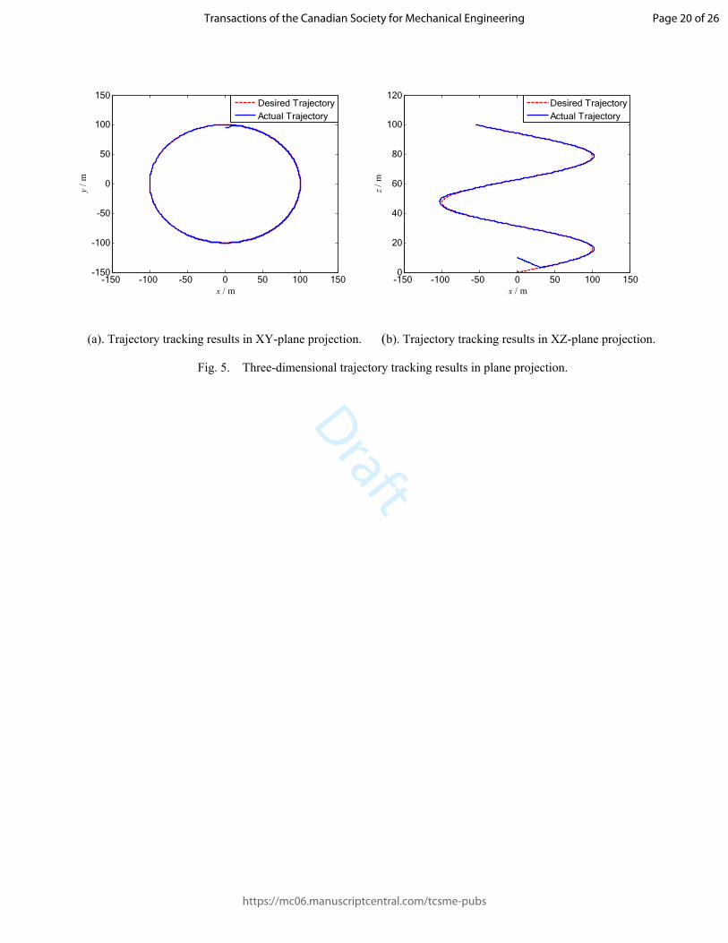
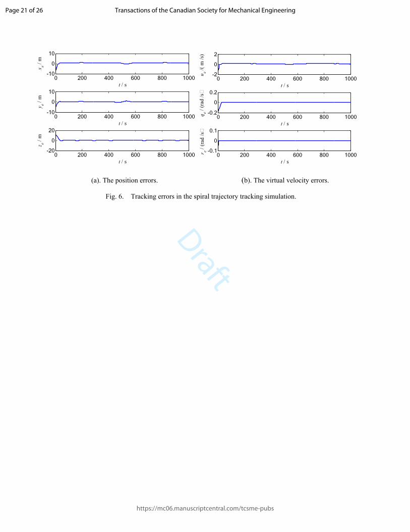
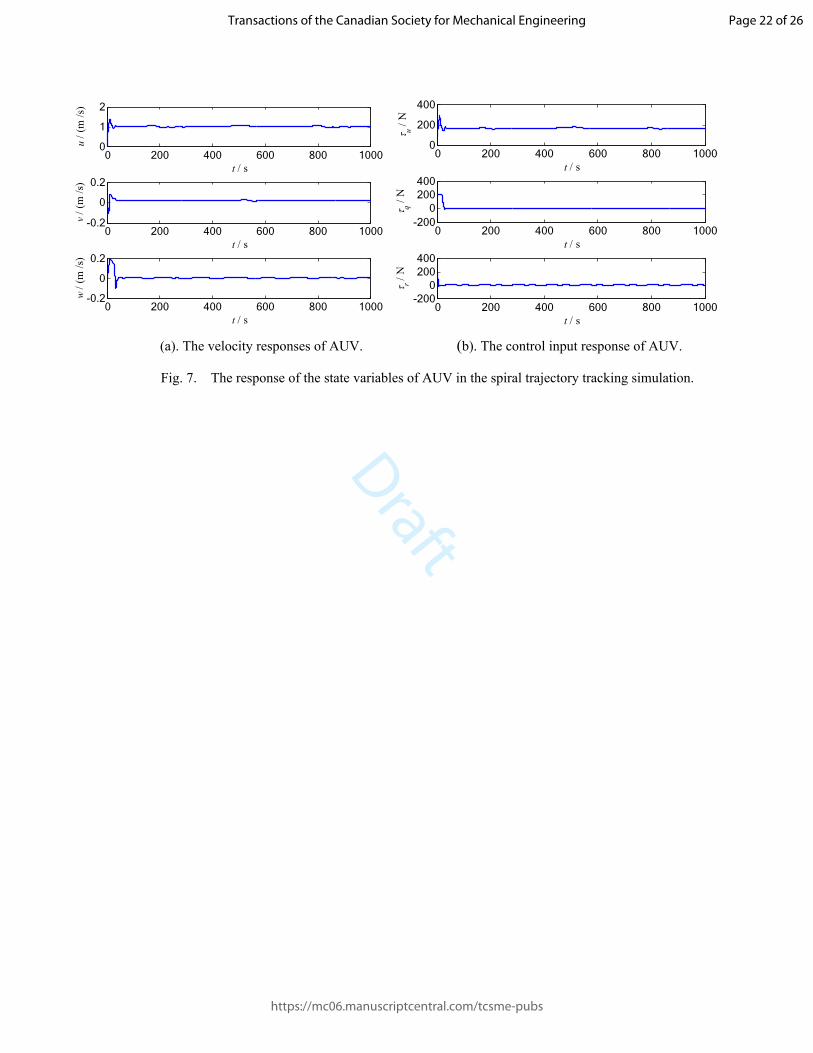
Fig. 4 and Fig. 5 are the simulation results of trajectory tracking and their planar projections. As vividly shown in Fig. 4- 5, the AUV realizes the tracking of the given spiral trajectory in the presence of a large initial position error. Fig. 6 shows the tracking errors in the spiral trajectory tracking simulation. It can be seen from Fig. 6(a) that the position errors of the AUV gradually converges to zero around 35s and there is no obvious overshoot and oscillation, which indicates the designed control law is not only has good tracking performance but also have robustness against parameters perturbation and ocean current disturbances. Fig. 6(b) shows the virtual velocity errors, and it can be seen that the dynamic control law can quickly stabilize the virtual velocity errors eu , eq and er , that is, the AUV is driven to have the desired velocities required to track the given trajectories. Fig. 7(a) shows the velocity responses of the AUV. We can know that the sway velocity 0.1m/sv ≈ and the heave velocity 0m/sw ≈ , and it is clear that both v and w are bounded which verifies the correctness of the lemma1. Fig. 7(b) is the responses of the control inputs uτ , qτ and rτ of the AUV, i.e. the output response of the dynamic control law. In order to overcome the disturbances, the control inputs have slight oscillation, but overall it is relatively smooth and stable and no chattering phenomenon occurs.
Case 2: Cosine trajectory tracking The desired trajectory in Zhou et al. (2017) is a combination of a straight line and a spiral curve, and the
desired velocities of the AUV are constant. That is, it is actually a relatively simple constant velocity control, which blurs the boundary between the trajectory tracking control and the path following control. To further verify the adaptability of the control algorithm, the desired cosine trajectory is given as:
m100cos(0.01 ) m100 100cos(0.01 ) m
d
d
d
x ty tz t
= = = −
(35)
The initial states of the AUV are set as [ (0), (0), (0), (0), (0)] [0(m),100(m), 30(m), 0(rad), 0(rad)]T Tx y z q y = ;
[ (0), (0), (0)] [0(m / s), 0(m / s), 0(m / s)]T Tu v w = ; [ (0), (0)] [0(rad / s), 0(rad / s)]T Tq r = .
Fig. 8.
(a). (b).
Fig. 9.
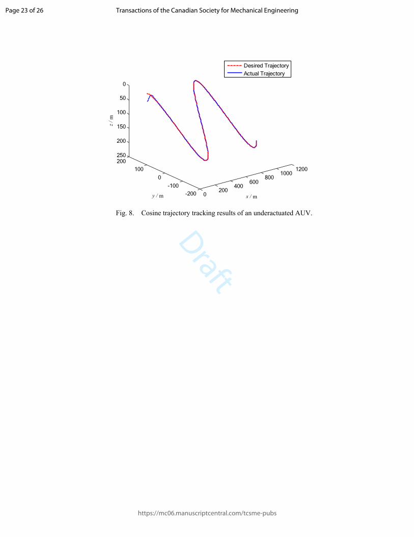
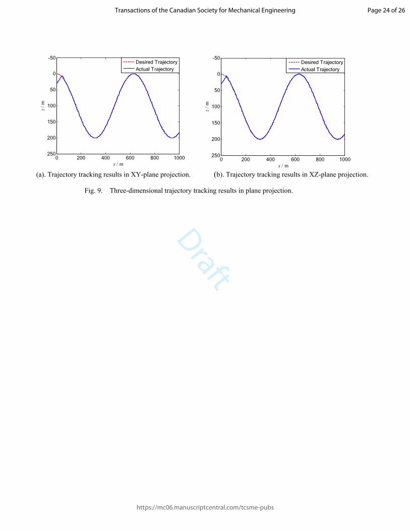
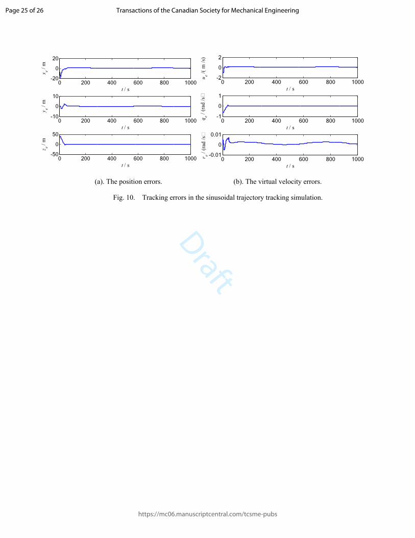
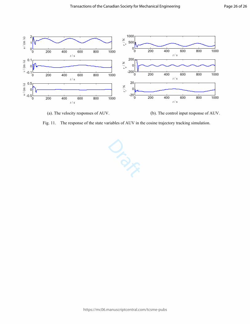
Compared with the spiral trajectory tracking, the desired velocity of the cosine trajectory is time-varying which requires the control algorithm to have stronger robustness. As shown in Fig. 8-9, the AUV accurately tracks the given cosine trajectory in the presence of a large initial position error. It can be seen from Fig.10 that the position errors and the virtual velocity errors are gradually converges to zero in finite time. Figure 11 shows the velocity response and the control inputs response of the AUV, as can be seen that the control inputs are reasonable and there is no obvious chattering phenomenon. This control algorithm has a low requirement for the AUV's actuators, which explains the practical feasibility of the control algorithm to some extent.
(a). (b).
Fig. 10.
Page 11 of 26
https://mc06.manuscriptcentral.com/tcsme-pubs
Transactions of the Canadian Society for Mechanical Engineering
Draft
(a). (b). Fig. 11.
Based on the above simulation results and analysis, the trajectory tracking control algorithm for an underactuated AUV designed in this paper has good comprehensive tracking performance and robustness. Compared with the control algorithm proposed in Zhou et al. (2017), the algorithm designed in this paper has better adaptability and practical feasibility.
5. Conclusions
Considering the three-dimensional trajectory tracking problem of underactuated AUV, a trajectory tracking control algorithm was designed based on the backstepping and sliding mode control methods. The effectiveness and robustness of the control algorithm were verified by the two typical simulations, which are spiral trajectory tracking and cosine trajectory tracking. The control algorithm combines the backstepping and the sliding mode control effectively to compensate for the lack of robustness of the backstepping method. At the same time, it overcomes the chattering problem which is common in the traditional sliding mode control. The control algorithm has lower requirements for the actuators of the underactuated AUV, which has good practical feasibility.
Acknowledgments
This work was supported by the National Nature Science Foundation of China (Nos. 51579024, 51879027, 51809028, 61374114) and the Fundamental Research Funds for the Central Universities (Nos. 3132016311, 3132018128).
References
Aguiar A.P., and Hespanha J.P. 2007. Trajectory-Tracking and Path-Following of Underactuated Autonomous Vehicles With Parametric Modeling Uncertainty. IEEE Transactions on Automatic Control, 52(8):1362-1379. https://doi.org/10.1109/TAC.2007.902731.
Bouzid Y., Siguerdidjane H., and Bestaoui Y. 2016. Improved 3D trajectory tracking by Nonlinear Internal Model-Feedback linearization control strategy for autonomous systems. IFAC-Papers- OnLine, 49(9):13-18. https://doi.org/10.1016/j.ifacol.2016.07.480.
Cui R., Chen L., Yang C., and Chen M. 2017. Extended State Observer-Based Integral Sliding Mode Control for an Underwater Robot with Unknown Disturbances and Uncertain Nonlinearities. IEEE Transactions on Industrial Electronics, 64(8):6785-6795. https://doi.org/10.1109/TIE.2017.2694410.
Cui R., Zhang X., and Cui D. 2016. Adaptive sliding-mode attitude control for autonomous underwater vehicles with input nonlinearities. Ocean Engineering, 123:45-54. https://doi.org/10.1016/j.oceaneng.2016.06.041.
Casau P., Sanfelice R.G., Cunha R., Cabecinhas, D., and Silvestre C. 2015. Robust global trajectory tracking for a class of underactuated vehicles. Automatica, 58:90-98. https://doi.org/10.1016/j.automatica.2015.05.011.
Chen Y., Zhang R., Zhao X., and Gao Z. 2016. Adaptive fuzzy inverse trajectory tracking control of underactuated underwater vehicle with uncertainties. Ocean Engineering, 121:123-133. https://doi.org/10.1016/j.oceaneng.2016.05.034.
Page 12 of 26
https://mc06.manuscriptcentral.com/tcsme-pubs
Transactions of the Canadian Society for Mechanical Engineering
Do K.D. 2015. Global robust adaptive path-tracking control of underactuated ships under stochastic disturbances. Ocean Engineering, 111:267-278. https://doi.org/10.1016/j.oceaneng.2015.10.038.
Dong Z., Wan L., Li Y., Liu T, and Zhang G. 2015. Trajectory tracking control of underactuated USV based on modified backstepping approach. International Journal of Naval Architecture & Ocean Engineering, 7(5):817-832. https://doi.org/10.1515/ijnaoe-2015-0058.
Elmokadem T., Zribi M., and Youcef-Toumi K. 2016. Terminal sliding mode control for the trajectory tracking of underactuated Autonomous Underwater Vehicles. Ocean Engineering, 129:613-625. https://doi.org/10.1016/j.oceaneng.2016.10.032.
Fakhreddin A., Malik A.H, and Norihan M.A. Lyapunov function for nonuniform in time global asymptotic stability in probability with application to feedback stabilization. Acta Applicandae Mathematicae, 106(1):1107-117. https://doi.org/10.1007/s10440-011-9632-8.
Fossen T.I. 2011. Handbook of marine craft hydrodynamics and motion control. New York, USA: John Wiley and Sons Ltd.
Huang J., Wen C., Wang W., and Song Y.D. 2015. Global stable tracking control of underactuated ships with input saturation. Systems & Control Letters, 85:1-7. https://doi.org/10.1016/j.sysconle.2015.07.002.
Karkoub M., Wu H.M., and Hwang C.L. 2017. Nonlinear trajectory-tracking control of an autonomous underwater vehicle. Ocean Engineering, 145:188-198. https://doi.org/10.1016/j.oceaneng.2017.08.025.
Luis J., Clement B., and Garelli F. 2016. Sliding mode reference conditioning for path following applied to an AUV. IFAC-Papersonline, 49(23):8-13. https://doi.org/10.1016/j.ifacol.2016.10.314.
Liu Y.C., Liu S.Y. and Wang N. 2016. Fully-tuned fuzzy neural network based robust adaptive tracking control of unmanned underwater vehicle with thruster dynamics. Neurocomputing, 196:1-13. https://doi.org/10.1016/j.neucom.2016.02.042.
Liang X., Wan L., Blake J.I.R., Shenoi R.A., and Towmsend N. 2016. Path Following of an Underactuated AUV Based on Fuzzy Backstepping Sliding Mode Control. International Journal of Advanced Robotic Systems, 13(3):1-11. https://doi.org/10.5772/64065.
Park B.S. 2017. A simple output-feedback control for trajectory tracking of underactuated surface vessels. Ocean Engineering, 143:133-139. https://doi.org/10.1016/j.oceaneng.2017.07.058.
Qiao L., Yi B., Wu D., and Zhang W. 2017. Design of three exponentially convergent robust controllers for the trajectory tracking of autonomous underwater vehicles. Ocean Engineering, 134:157-172. https://doi.org/10.1016/j.oceaneng.2017.02.006.
Qiao L., and Zhang W.D. 2018. Adaptive second-order fast nonsingular terminal sliding mode tracking control for fully actuated autonomous underwater vehicles. IEEE Journal of Oceanic Engineering, pp.1-23. https://doi.org/10.1109/JOE.2018.2809018.
Rezazadegan F., Shojaei K., Sheikholeslam F., and Chatraei A. 2015. A novel approach to 6-DOF adaptive trajectory tracking control of an AUV in the presence of parameter uncertainties. Ocean Engineering, 107(1):246-258. https://doi.org/10.1016/j.oceaneng.2015.07.040.
Repoulias F., and Papadopoulos E. 2007. Planar trajectory planning and tracking control design for underactuated AUVs. Ocean Engineering, 34(11):1650-1667. https://doi.org/10.1016/j.oceaneng.2006.11.007.
Shojaei K. 2017. Three-dimensional neural network tracking control of a moving target by underactuated autonomous underwater vehicles. Neural Computing & Applications, 1:1-13. https://doi.org/10.1007/s00521-017-3085-6.
Page 13 of 26
https://mc06.manuscriptcentral.com/tcsme-pubs
Transactions of the Canadian Society for Mechanical Engineering
Sahu B.K., and Subudhi B. 2014. Adaptive tracking control of an autonomous underwater vehicle. International Journal of Automation and Computing, 11(3):299-307. https://doi.org/10.1007/s11633-014-0792-7.
Xu J., Wang M., and Qiao L.2015. Dynamical sliding mode control for the trajectory tracking of underactuated unmanned underwater vehicles. Ocean Engineering, 105:54-63. https://doi.org/10.1016/j.oceaneng.2015.06.022.
Yan Z., Yu H., Zhang W., Li B., and Zhou J. 2015. Globally finite-time stable tracking control of underactuated UUVs. Ocean Engineering, 107:132-146. https://doi.org/10.1016/j.oceaneng.2015.07.039.
Yu R., Zhu Q., Xia G., and Liu Z. 2012. Sliding mode tracking control of an underactuated surface vessel. Iet Control Theory & Applications, 6(3):461-466. https://doi.org/10.1049/iet-cta.2011.0176.
Zakeri E., Farahat S., Moezi S.A., and Zare A. 2016. Robust sliding mode control of a mini unmanned underwater vehicle equipped with a new arrangement of water jet propulsions: Simulation and experimental study. Applied Ocean Research, 59:521-542. https://doi.org/10.1016/j.apor.2016.07.006.
Zhu G., Du J., and Kao Y. 2018. Command filtered robust adaptive NN control for a class of uncertain strict-feedback nonlinear systems under input saturation. Journal of the Franklin Institute, 2018, 355(15):7548-7569. https://doi.org/10.1016/j.jfranklin.2018.07.033.
Zheng Z., Jin C., Zhu M., and Sun K. 2015. Trajectory tracking control for a marine surface vessel with asymmetric saturation actuators. Robotics & Autonomous Systems, 97:83-91. https://doi.org/10.1016/j.robot.2017.08.005.
Zhang Z., and Wu Y. 2015. Further results on global stabilization and tracking control for underactuated surface vessels with non-diagonal inertia and damping matrices. International Journal of Control, 88(9):1679-1692. https://doi.org/10.1080/00207179.2015.1013061.
Zhou J., Ye D., Zhao J., and He D. 2017. Three-dimensional trajectory tracking for underactuated AUVs with bio-inspired velocity regulation. International Journal of Naval Architecture & Ocean Engineering, pp.1-12. https://doi.org/10.1016/j.ijnaoe.2017.08.006. Caption list of figures: Fig. 1. The coordination frames of AUV.
Fig. 2. The schematic of the proposed three-dimensional trajectory tracking control system.
Fig. 3. The response curves of the function sgn(.) and tanh(.).
Fig. 4. Spiral trajectory tracking results of an underactuated AUV.
Fig. 5. Three-dimensional trajectory tracking results in plane projection.
(a). Trajectory tracking results in XY-plane projection. (b). Trajectory tracking results in XZ-plane projection.
Fig. 6. Tracking errors in the spiral trajectory tracking simulation.
(a). The position errors. (b). The virtual velocity errors.
Fig. 7. The response of the state variables of AUV in the spiral trajectory tracking simulation.
(a). The velocity responses of AUV. (b). The control input response of AUV.
Page 14 of 26
https://mc06.manuscriptcentral.com/tcsme-pubs
Transactions of the Canadian Society for Mechanical Engineering