Purdue UniversityPurdue e-Pubs

Open Access Dissertations Theses and Dissertations

January 2016

Three Dimensional Unsteady Flow and ActiveMorphing Effect in Flapping WingsYun LiuPurdue University

Follow this and additional works at: https://docs.lib.purdue.edu/open_access_dissertations

This document has been made available through Purdue e-Pubs, a service of the Purdue University Libraries. Please contact epubs@purdue.edu foradditional information.

Recommended CitationLiu, Yun, "Three Dimensional Unsteady Flow and Active Morphing Effect in Flapping Wings" (2016). Open Access Dissertations. 1391.https://docs.lib.purdue.edu/open_access_dissertations/1391

THREE DIMENSIONAL UNSTEADY FLOW

AND

ACTIVE MORPHING EFFECT

IN

FLAPPING WINGS

A Dissertation

Submitted to the Faculty

of

Purdue University

by

Yun Liu

In Partial Fulfillment of the

Requirements for the Degree

of

Doctor of Philosophy

August 2016

Purdue University

West Lafayette, Indiana

ii

ACKNOWLEDGMENTS

First, I want to express my deep gratitude to Dr. Xinyan Deng for her constant

and encouraging support and guidance which were essential to my research through

all these five years.

Especially, I want to thank Dr. Bo Cheng, a close colleague and friend, for his

critical input and comments on Chapters 2, 3, and 4. During the writing of Chapter

5, I was very much benefited from the comments and discussions with Mr Jesse Roll

who was also very kind in helping me on experimental setups in different projects. I

further want to thank Dr Haibo Dong from University of Virginia and Dr Sanjay.P

Sane from National Center for Biological Sciences of India for their kind input and

comments.

Lastly, I would like to thank my grandfather Shuren Liu for his inspiring words and

spirits that motivated me to accomplish every goal during this journey of searching

and exploring.

iii

TABLE OF CONTENTS

Page

LIST OF TABLES . . . . . . . . . . . . . . . . . . . . . . . . . . . . . . . . iv

LIST OF FIGURES . . . . . . . . . . . . . . . . . . . . . . . . . . . . . . . v

ABBREVIATIONS . . . . . . . . . . . . . . . . . . . . . . . . . . . . . . . . vi

ABSTRACT . . . . . . . . . . . . . . . . . . . . . . . . . . . . . . . . . . . vii

LIST OF PUBLICATIONS . . . . . . . . . . . . . . . . . . . . . . . . . . . ix

1. INTRODUCTION . . . . . . . . . . . . . . . . . . . . . . . . . . . . . . 11.1 Background Overview . . . . . . . . . . . . . . . . . . . . . . . . . 11.2 Three fundamental features on the aerodynamics of insect flight . . 51.3 Outline of the thesis . . . . . . . . . . . . . . . . . . . . . . . . . . 10

2. VOLUMETRIC VISUALIZATION OF THE NEAR- AND FAR-FIELD WAKEIN FLAPPING WINGS . . . . . . . . . . . . . . . . . . . . . . . . . . . 132.1 Chapter Abstract . . . . . . . . . . . . . . . . . . . . . . . . . . . . 132.2 Introduction . . . . . . . . . . . . . . . . . . . . . . . . . . . . . . . 132.3 Materials and Methods . . . . . . . . . . . . . . . . . . . . . . . . . 152.4 Results . . . . . . . . . . . . . . . . . . . . . . . . . . . . . . . . . . 182.5 Conclusion and Discussion . . . . . . . . . . . . . . . . . . . . . . . 23

3. AERODYNAMICS OF DYNAMIC WING FLEXION IN TRANSLATINGWINGS . . . . . . . . . . . . . . . . . . . . . . . . . . . . . . . . . . . . 253.1 Chapter Abstract . . . . . . . . . . . . . . . . . . . . . . . . . . . . 253.2 Introduction . . . . . . . . . . . . . . . . . . . . . . . . . . . . . . . 263.3 Experimental setup and Procedure . . . . . . . . . . . . . . . . . . 283.4 Results and Discussion . . . . . . . . . . . . . . . . . . . . . . . . . 32

3.4.1 Instantaneous Force . . . . . . . . . . . . . . . . . . . . . . . 343.4.2 Average Force . . . . . . . . . . . . . . . . . . . . . . . . . . 363.4.3 Flow patterns and Circulation . . . . . . . . . . . . . . . . . 393.4.4 Vortex strength and lift peak . . . . . . . . . . . . . . . . . 45

3.5 Concluding remarks . . . . . . . . . . . . . . . . . . . . . . . . . . . 47

4. CONVENTIONAL FLOW VISUALIZATIONS ON MECHANICAL FLAP-PERS . . . . . . . . . . . . . . . . . . . . . . . . . . . . . . . . . . . . . 504.1 An Application of Smoke Wire Visualization on a Hovering Insect Wing 50

4.1.1 Introduction . . . . . . . . . . . . . . . . . . . . . . . . . . . 504.1.2 Experimental Method . . . . . . . . . . . . . . . . . . . . . 50

iv

Page4.1.3 Results and Discussion . . . . . . . . . . . . . . . . . . . . . 51

4.2 Dye Visualization on a Mechanical Flapping Wing . . . . . . . . . . 544.2.1 Introduction . . . . . . . . . . . . . . . . . . . . . . . . . . . 544.2.2 Experimental Method . . . . . . . . . . . . . . . . . . . . . 544.2.3 Results and Discussion . . . . . . . . . . . . . . . . . . . . . 55

5. INSECTS FLY ON LADDERS OF VORTICES . . . . . . . . . . . . . . 575.1 Chapter Abstract . . . . . . . . . . . . . . . . . . . . . . . . . . . . 575.2 Results and Discussion . . . . . . . . . . . . . . . . . . . . . . . . . 585.3 Method . . . . . . . . . . . . . . . . . . . . . . . . . . . . . . . . . 66

6. SUMMARY . . . . . . . . . . . . . . . . . . . . . . . . . . . . . . . . . . 69

A. APPENDIX . . . . . . . . . . . . . . . . . . . . . . . . . . . . . . . . . . 76A.1 Flow Uncertainty . . . . . . . . . . . . . . . . . . . . . . . . . . . . 76A.2 Force Uncertainty . . . . . . . . . . . . . . . . . . . . . . . . . . . . 77

LIST OF REFERENCES . . . . . . . . . . . . . . . . . . . . . . . . . . . . 80

VITA . . . . . . . . . . . . . . . . . . . . . . . . . . . . . . . . . . . . . . . 87

v

LIST OF TABLES

Table Page

3.1 Flexion duration versus trailing-edge velocity magnitude due to flexion 29

vi

LIST OF FIGURES

Figure Page

1.1 Smoke Visualization on tethered Hawkmoth(Ellington et al 1996) . . . 2

1.2 Top and side views of CFD-visualized flows with instantaneous streamlinesand surface pressure contours during supination(Liu et al 1998) . . . . 4

1.3 2D flow visualization on translating plate(Dickinson and Gotz 1993) . . 6

1.4 Instantaneous flow measurement on a tethered locust,using tomographicPIV(Henningsson et al 2015) . . . . . . . . . . . . . . . . . . . . . . . . 8

1.5 Left wing of Eristalis tenax, showing the attachment of the alula (Walkeret al 2012) . . . . . . . . . . . . . . . . . . . . . . . . . . . . . . . . . . 9

1.6 Three basic features in aerodynamics of insect flight . . . . . . . . . . . 11

2.1 Experimental Setup (a) Schematics of the servo driven mechanical flapperand the measurement volume of the V3V system. (b) Wing profile. (c)Measured stroke and rotation angle (b) Wing stroke positions where thevelocity field was measured. . . . . . . . . . . . . . . . . . . . . . . . . 17

2.2 Isosurfaces of vorticity magnitude |ω| at wing stroke position #0. (a) Twoisosurfaces with |ω|= 4/s (yellow) and |ω|= 10/s (green). (b) The RGBcolor-coded (red, ωx; green, ωy; blue ωz) isosurface (|ω|= 10/s) showingtwo linked vortex rings. (c) The RGB color-coded isosurface (|ω|= 4/s)showing two parallel shear layers. Left and right columns show the sameisosurfaces at two different views . . . . . . . . . . . . . . . . . . . . . 20

2.3 Vorticity and velocity distribution at wing stroke position 0. (a) 2D slicesshowing Z vorticity contour and streamlines at Z = -720 and -750 mm,and isosurface of vorticity magnitude at with |ω|= 4/s. (b) Isosurface ofvelocity magnitude (red) at 8.5 cm/s, which is enclosed by the isosurfacesof vorticity magnitudes at |ω|= 4/s (yellow) and |ω|= 10/s (green). (c)Velocity vector field on the two perpendicular slices Z = -740mm and Y=45mm . . . . . . . . . . . . . . . . . . . . . . . . . . . . . . . . . . . . 21

vii

Figure Page

2.4 Isosurfaces of vorticity magnitude (|ω|= 10/s) and vorticity contour plotsat 8 different stroke positions, which demonstrate the evolution of thevortex wake structure. The contour plot of Z vorticity at X-Y plane (Z =-730 mm) shows the tip vortex (TV) and root vortex (RV) as well as twoshear layers in the far field. The contour plot of Y vorticity at X-Z plane(Y= 45mm) shows the leading edge vortex (LEV) and other vortices shedat stroke reversals. . . . . . . . . . . . . . . . . . . . . . . . . . . . . . 22

3.1 Schematics of the experimental setup and wing kinematics. (a) Experi-mental setup.(b) Wing model. Two wing sections of same chord lengthwere connected by two hinges. (c) Wing cross section with bluntly roundedleading edge and sharply taped trailing edge. A red rectangular region wasused to calculate the circulation around the wing. (d) Wing starts to trans-late at t = 0 s and accelerates to the final velocity of 0.1m/s within 0.4 s.Wing starts the flap deflection at t = tdelay s and deflect to a fixed angleof 40o within tspan s; tdelay controls the deflection timing and tspan controlsthe deflection speed. . . . . . . . . . . . . . . . . . . . . . . . . . . . . 30

3.2 Circulation magnitude of leading edge vortex and its corresponding freevortex as well as the trailing edge vortex and its corresponding statingvortex during the onset of wing translation. Trailing edge vortex stopsgrowing and begins to shed at t= 0.5 s (red curve); Leading edge vortexstops growing and starts to shed at t 1.1 s (green curve). . . . . . . . . 33

3.3 Instantaneous lift coefficient versus normalized time; Lift coefficient curvesunder the same deflection timing are plotted together in the same group(a-o). Black arrows indicate the instant when the wing starts to deflect.Black curves are the lift coefficient on the non-deflected flat wing whilethe other color coded curves present the lift coefficient on the wing withdifferent deflection speeds. . . . . . . . . . . . . . . . . . . . . . . . . . 35

3.4 Instantaneous drag coefficient versus normalized time. . . . . . . . . . . 36

3.5 Contour plots of average force as functions of tdelay∗ and tspan

∗. Greensquares present the sampling points for force measurement. (a) Increaseon average lift coefficient over tdelay

∗ < t∗ < tdelay∗ + 3.0. (b) Increase

on average drag coefficient tdelay∗ < t∗ < tdelay

∗ + 3.0. (c) Average liftcoefficient over −0.8 < t∗ < 8. Black circles present the sampling pointsfor flow measurement. (d) Average drag coefficient over −0.8 < t∗ < 8.(e) Average lift-drag ratio over −0.8 < t∗ < 8. (f) Geometry effect of flapdeflection on the lift-drag ratio. . . . . . . . . . . . . . . . . . . . . . . 38

viii

Figure Page

3.6 A typical flow in region I at tdelay∗ = −0.8 and tspan

∗ = 0.4 where the wingdeflects before the wing starts with a high deflection speed. (a-l) Contourplots of vorticity. Black parts present wings cross section; Red arrows givethe instantaneous net forces; Blue arrows show the translational velocityon the wing. (g) Negative vorticity was induced closed to hinge. (i) In-duced negative vorticity feeds into LEV. (j-l) LEV is promoted by feedingthe induced negative vorticity into LEV. (m) Region I highlighted by yel-low loop. Red circle and arrow indicate where current contour plots ofvorticity were measured. . . . . . . . . . . . . . . . . . . . . . . . . . 39

3.7 A typical flow in region II at tdelay∗ = 0.4 and tspan

∗ = 0.4 (b) SV wasenhanced by flap deflection and the net force had a significant increase.(h) Induced negative vorticity was feed into the LEV. (m) Region II withhigh average lift, highlighted by red loop. . . . . . . . . . . . . . . . . 41

3.8 A typical flow in region III at tdelay∗ = 1.4and tdelay

∗ = 0.8 (d) AnotherTEV was created by deflection beside SV. (j) Induced negative vorticityfeeds into LEV. . . . . . . . . . . . . . . . . . . . . . . . . . . . . . . . 42

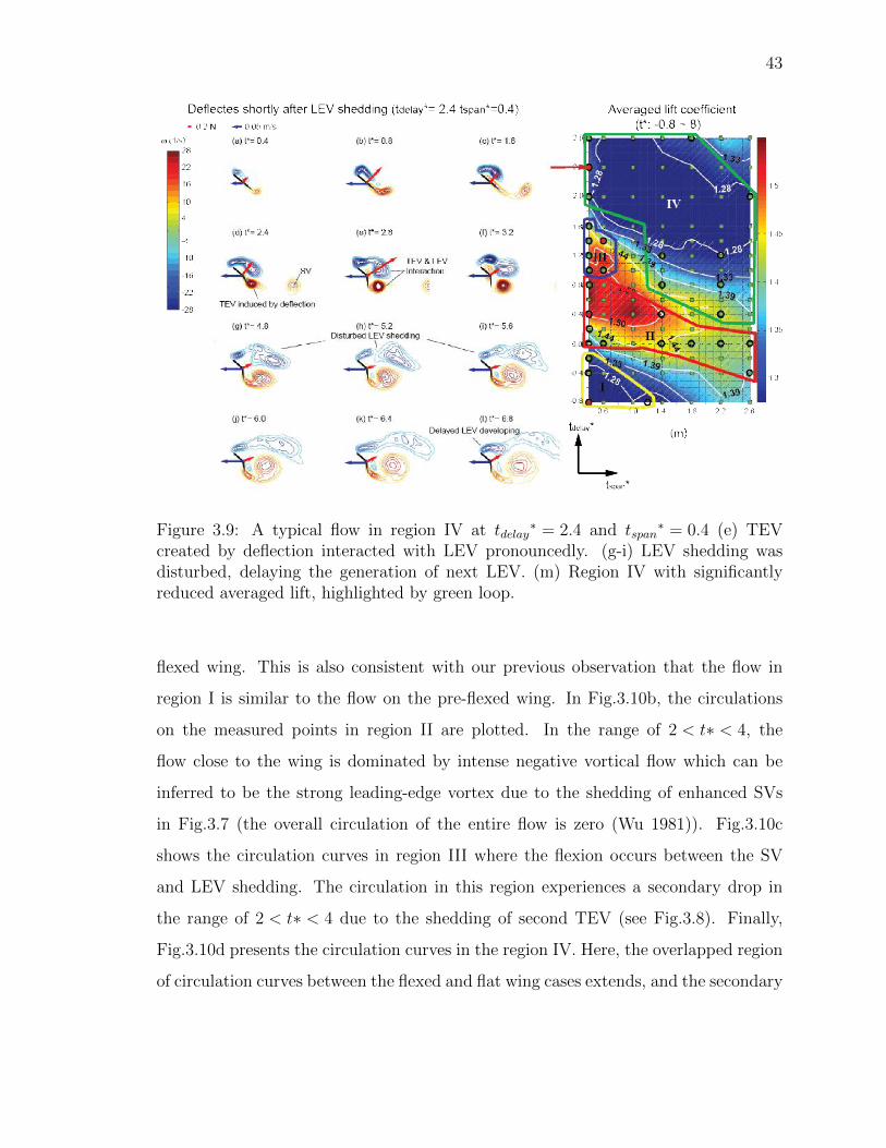
3.9 A typical flow in region IV at tdelay∗ = 2.4 and tspan

∗ = 0.4 (e) TEV cre-ated by deflection interacted with LEV pronouncedly. (g-i) LEV sheddingwas disturbed, delaying the generation of next LEV. (m) Region IV withsignificantly reduced averaged lift, highlighted by green loop. . . . . . . 43

3.10 Circulation versus normalized time. Circulation curves in the same regionhave similar behavior. (a) Circulation curves in region I overlap with eachother and are closed to the circulation on the pre-deflected wing (blackdash curve). (b) Circulation curves in region II have pronounced negativecirculation in the range of 2 < t∗ < 4. (c) Circulation curves in region IIIhave abrupt drops in the range of 2 < t∗ < 4. (d) Circulation curves inregion IV experience mild increase over 4 < t∗ < 6 and limited decreaseover 6 < t∗ < 7. . . . . . . . . . . . . . . . . . . . . . . . . . . . . . . . 44

3.11 Circulation magnitude of vortices on the deflected wings with the highestflexion speed (tspan

∗ = 0.4) but different flexion timings (−1 < tdelay∗ < 2.8))

versus normalized time. (a), (c) Circulation magnitude of LEVs/its corre-sponding free vortices and TEVs/SVs when wing flexion happens beforeSV shedding (b), (d) Circulation magnitude of vortices when wing flexionhappens after SV shedding . . . . . . . . . . . . . . . . . . . . . . . . . 47

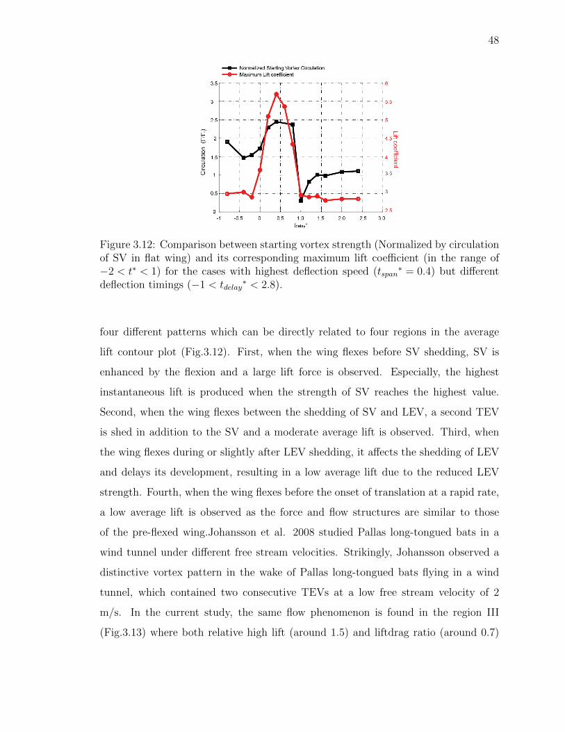
3.12 Comparison between starting vortex strength (Normalized by circulationof SV in flat wing) and its corresponding maximum lift coefficient (inthe range of −2 < t∗ < 1) for the cases with highest deflection speed(tspan

∗ = 0.4) but different deflection timings (−1 < tdelay∗ < 2.8). . . . 48

ix

Figure Page

3.13 A summary of active flexion effects on the flow and lift force. (a) Flowon non-deflected flat wing is simply dominated by a starting vortex in thebeginning and alternative vortices shedding afterward. (b) By adjust theactive flexion timing respected to the timings of vortices shedding (withmoderate flexion speed) four types of flow pattern can be produced (c)Four average lift regions can be closely related to the four different flowpatterns. . . . . . . . . . . . . . . . . . . . . . . . . . . . . . . . . . . . 49

4.1 Flapper with cicada wings . . . . . . . . . . . . . . . . . . . . . . . . . 51

4.2 The experimental setup . . . . . . . . . . . . . . . . . . . . . . . . . . 51

4.3 Smoke patterns showing the evolution of the flow structure in an upstroke(5 Hz), for more details refer to the video in the supplementary material. 52

4.4 Dye visualizaiton results on a mechanical flapper. . . . . . . . . . . . . 55

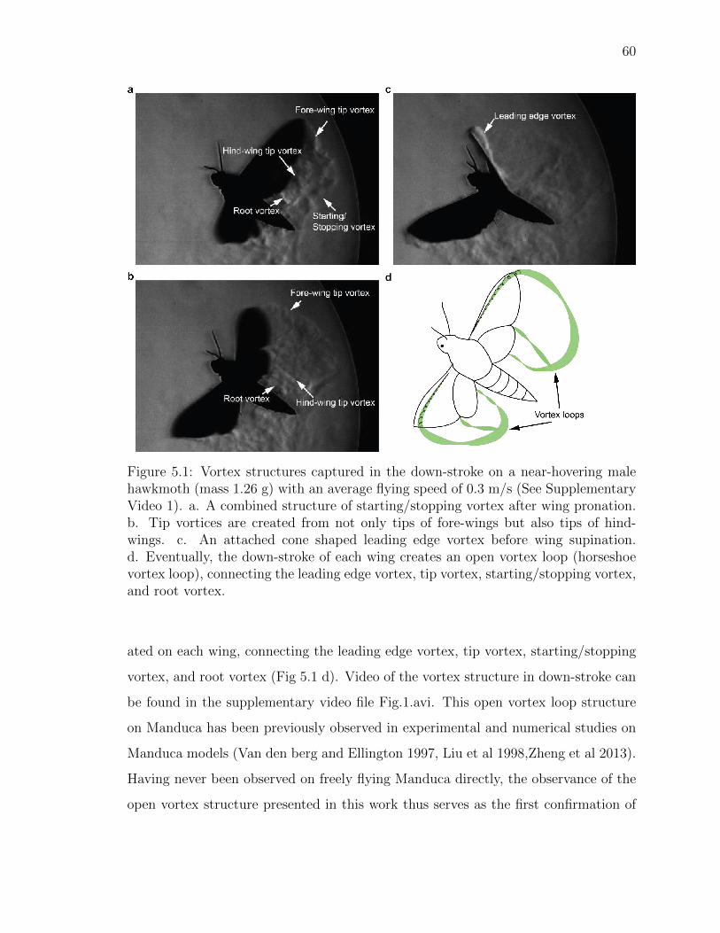
5.1 Vortex structures captured in the down-stroke on a near-hovering malehawkmoth (mass 1.26 g) with an average flying speed of 0.3 m/s (SeeSupplementary Video 1). a. A combined structure of starting/stoppingvortex after wing pronation. b. Tip vortices are created from not onlytips of fore-wings but also tips of hind-wings. c. An attached cone shapedleading edge vortex before wing supination. d. Eventually, the down-stroke of each wing creates an open vortex loop (horseshoe vortex loop),connecting the leading edge vortex, tip vortex, starting/stopping vortex,and root vortex. . . . . . . . . . . . . . . . . . . . . . . . . . . . . . . . 60

5.2 Vortex structures captured in the up-stroke on the near hovering hawk-moth (See Supplementary Video 2). a. The vortex loop created in down-stroke sheds into the wake. b-c Long, stretched tip vortices from the tipsof fore-wings and hind-wings are created and connected to the just shedvortex loops. d. Finally, the up-stroke of each wing creates long, stretchedtip and root vortices, connecting the shed vortex loop to the wing. . . . 62

x

Figure Page

5.3 Vortex structures from consecutive wing beat cycles are well linked. a-b.The vortex structure capured on an ascending male hawkmoth(mass 0.93g) with an average flying speed of 0.7m/s (left and right columns showthe flow structure filmed from front and side views). a. On the ascend-ing hawkmoth, a vortex loop is created on each wing in the down-strokeand the vortex loop is connected to the vortex structure creaed from thelast up-stroke.b.In the up-stroke, stretched hind-and fore-wing tip vor-tices as well as root vortex are created on each wing,connecting to thevortex loop from the down-stroke.c.Between consecutive wing beat cycles,a linked structure is also observed on the near hovering hawkmoth. Tipvortices from the up-stroke shed from the wings and connect to the start-ing/stopping vortices, thereby connecitng the vortex structures betweeneach wing beat cycle. Left image shows the original image of the strucutreand right image shows notated vortex structure. . . . . . . . . . . . . . 63

5.4 Vortex ladder under an ascending hawkmoth. a. In the down-stroke, avortex loop is created and linked to the other vortex loops through tip androot vortices formed from up-strokes, forming a ladder of vortices undereach wing. b. In the up-stroke, stretched tip and root vortices are createdon each wing connecting the just shed vortex loop to the wing. . . . . . 64

5.5 Experimental Setup . . . . . . . . . . . . . . . . . . . . . . . . . . . . . 67

6.1 Secondary hind-wing tip vortex on a butterfly(images were shot in a se-quence from a to d) . . . . . . . . . . . . . . . . . . . . . . . . . . . . . 72

6.2 An explaination of the Secondary Tip vortex. Leading edge vortex strengthis not evenly distributed with vortex filaments shed not evenly, creating asecondary vortex somewhere from wing root to tip. The red loops indicatethe vortex structures created in down-stroke and vortex structure createdin up-stroke is in blue . . . . . . . . . . . . . . . . . . . . . . . . . . . 73

6.3 High speed Schlieren photography on a tethered Wasps . . . . . . . . . 74

6.4 High speed Schlieren photography on a falling plate . . . . . . . . . . . 75

xi

ABBREVIATIONS

AoA Angle of Attack

LEV Leading edge vortex

TEV Trailing edge vortex

TV Tip vortex

RV Root vortex

SV Starting vortex

φ Stroke angle

ψ Rotational angel

ω vorticity

δ flexion angle

Γ Circlation

tdelay time delay between wing translation and flexion

tspan time required for wing flexion

xii

ABSTRACT

Liu, Yun PhD, Purdue University, August 2016. Three Dimensional Unsteady Flowand Active Morphing Effect in Flapping Wings. Major Professor: Xinyan Deng,School of Mechanical Engineering.

Bumble bee cannot fly, if we ignore the significant differences between flapping

wings and fixed wings, and falsely apply the conventional fixed wing aerodynamic

principles to the bumble bee flight. The classic fixed wing aerodynamics originated

from the two-dimensional attached flow analysis, where the three-dimensional and

unsteady effects can be ignored without introducing too much error. Insects and

hummingbirds, however, flap their low aspect ratio and highly deformable wings

reciprocally, creating very complex flow structures, which are highly three-dimensional

and unsteady. In the meanwhile, the flexibility and complex textures of the wings

introduce even more complexities to the problem from the aspect of aero-elasticity.

Therefore, to see the entire picture of flapping wing aerodynamics, the three factors:

unsteadiness, three-dimensional effect and wing morphing have to be taken

into account and this thesis aims to provide some understanding about those issues

and the couplings related to them.

The state of art V3V system was used to study the coupling between unsteadi-

ness and three-dimensional effect of the flow on a mechanical flapper with rigid

wings, revealing a linked vortex ring structure in the near field with two layers of

strong vortical flow in the far field. On the other hand, the coupling of unsteadi-

ness and wing morphing was studied on a quasi-2-dimensional translating wing

with an active trailing edge flap, suggesting both the flow and force characteristics

were greatly affected by the flap deflection timing. Finally, to study the coupling of all

the three factors: unsteadiness, three-dimensional effect and wing morphing,

a new method of flow visualization was successfully developed and applied to freely

xiii

flying hawkmoth. For the first time, the entirety of the highly three-dimensional and

unsteady vortex structure was observed and reported experimentally on a freely flying

insect.

xiv

LIST OF PUBLICATIONS

Y Liu,J Roll, S.M. Van Kootan, S P. Sane, X Deng, Insect fly on ladders of

vortices. Submitted

Y Liu,B Cheng, S P. Sane, X Deng, Aerodynamics of dynamic wing flexion in

translating wings. Exp.Fluids. 56:131, 2015

B Cheng,J Roll,Y Liu, D R Troolin, X Deng, Three-dimensional vortex wake

structure of flapping wing in hovering flight. J.R.Soc.Interface. 11(91), 2014

Y Liu,B Cheng,X Deng, An application of smoke-wire visualization on a hovering

insect wing. J.Vis. 16(3),185-187, 2013

Y Liu,B Cheng,G Barbera, D RTrooling, X Deng,Volumetric Visualization of the

near- and far- field wake in flapping wings. Bioinspir.Biomom. 8,2013

Y Liu,B Cheng, X Deng, An experimental study of dynamic trailing edge de-

flections on a two-dimensional translating wings. 31st AIAA Applied Aerodynamic

Conference AIAA 2013-2816

1

1. INTRODUCTION

1.1 Background Overview

Lifting-line and airfoil theories, developed in the early 20th century, opened a new

era of fluid mechanics and paved the foundation of modern aerodynamics. Before the

1950s, without the modern computer technology, lifting-line and airfoil theories were

the most fundamental guidelines in aircraft designing and optimization(Anderson

1999). In the light of advancements of the fixed wing aerodynamic theories, aircraft

designing experienced booming and significant advancement in the early 20th century.

The fixed wing aerodynamic theories were so successful that people intended to use

these theories to study the aerodynamics of flying insects without considering the

fundamental difference between fixed and flapping wings (Bomphrey et al 2009). The

well-known “bumble bee cannot fly story” about the discussion between an aeronautic

engineer and a biologist then became a major motivation behind the over a century

research interests on insect flight (Bomphrey et al 2009, Sane 2003). Insect wings

translate and rotate at quite a high angle of attack where the flow already separates

from the fixed wings, resulting in a high drag but low lift force. Subsequently, the

lift force is greatly underestimated, if using the aerodynamic force data derived from

classic fixed wing aerodynamics, creating a false paradox that bumble bee cannot fly

(Bomphrey et al 2009).

On a small chalcid wasp, Encarsia Formosa, Weis-Fogh found and proposed the

“Clap-Fling” mechanism attributing to lift augmentation(Weis-Fogh 1973). By creat-

ing two bound vortices with opposite signs on the wings after pronation,“Clap-Fling”

can prevent the formation of starting vortices to eliminate the Wagner effect which

tends to weaken lift generation. However, this novel mechanism is only found in

limited insect species such as butterflies with a great range of insects not having

2

“Clap-Fling” mechanisms captured in their flights. After Weis-Fogh, C.P. Ellingtion

inherited his legacy and continued the research to determine the legitimate cause of

high lift production in insect flight.

Figure 1.1: Smoke Visualization on tethered Hawkmoth(Ellington et al 1996)

Utilizing the smoke visualization on the tethered Hawkmoth, Manduca sexta, as

well as a hawkmoth mimicking mechanical flapper (which not only can mimic the wing

trajectory but also the flexibility of the hawkmoth wings), a cone shaped leading edge

vortex (LEV) was captured and visualized (Ellington et al 1996,Van den berg and

Ellington 1997). Most significantly, Ellington clearly linked this finding of stable LEV

structure to the cause of high lift production which cannot be fully explained through

classic fixed wing aerodynamics, thereby providing one explanation to the paradox

that a bumble bee cannot fly. Through the discovery of LEV on the hawkmoth,

Ellington may have provided the final answer to the unexpected high lift generation

in insect flight while his work also brought more interesting aspects and questions

about LEV which is currently believed to be the major cause of lift augmentation

on animal flight. In addition, a great amount of research attention and interest

was drawn into the mechanism about stabilizing the LEV on the wing (Birch and

Dickinson 2001). Many theories and hypothesis were proposed, leading to an endless

debate over this topic (Lentink and Dickinson 2009, Cheng et al 2013). Within these,

a research group from Caltech, led by Prof. Dickinson, advanced the research on

3

insect flight to a higher level by studying the aerodynamics of fruit flies (Dickinson

et al 1999).

Considering the wings of the fruit fly as rigid wings, Dickinson and his colleagues

built a scaled up mechanical flapper-Robofly,that flapped at a much lower frequency

in an oil tank to dynamically simulate the flying fruit fly in the air. By measuring

the flow on the wing, Dickinson confirmed Ellington's finding about the existence of

LEV, but found no relevance about the span-wise flow and LEV stability which is

highlighted in Ellington's experimental results on the hawkmoth (Birch and Dickinson

2001). Furthermore, through systematic and detailed force and flow measurements on

the Robofly, Dickinson and his colleagues built the first mature aerodynamics model

that can estimate the aerodynamic force on flapping wings (Dickinson et al 1999).

Although the quasi-steady model is empirical and experimental data dependent, it

provides a sound and accurate force prediction.

In light of advancements in Computational Fluid Dynamics (CFD) and massive

fast computation capacities, simulating flow and dynamics on flying insects became

possible through solving the Navier-Stokes equation numerically. From simulations on

flying hawkmoth to fruit flies, Liu (Liu et al 1998,Aono et al 2008) depicted very com-

plex highly three-dimensional and unsteady flow structures on flying insects. Chal-

lenges in the simulation of insect flight stem from the complex nature of reciprocal

flapping wing motion and wing geometries. Three-dimensional dynamic and adaptive

mesh were used to cope with the complex wing motion that requred constructing new

mesh for calculation at each time step (Liu et al 1998). Later, by introducing the

immersed boundary method (IBM) to CFD simulations of insect flight, the mesh was

greatly simplified without considering too many geometric complexities (Mittal et al

2006). Moreover, instead of solving the Navier-Stokes equation, the Lattice Boltz-

mann Method was implemented to study the low Reynolds number flow problems,

like flapping wings (Li and Lu 2012). However, none of these simulations can per-

fectly simulate a flying insect by considering all the details from wing morphology to

wing texture. Therefore, all these CFD simulations are still based on more or less

4

Figure 1.2: Top and side views of CFD-visualized flows with instantaneous streamlinesand surface pressure contours during supination(Liu et al 1998)

simplified flying insect models which might neglect some important features on real

flying insects (this issue will be addressed in Chapter 5).

In the recent decade, with the advancement of three-dimensional flow measure-

ment/visualization methods, a much clearer picture about the flow in insect flight can

be obtained not only on insect mimicking mechanical flappers but also on real flying

insects (Liu et al 2013, Henningsson et al 2015). With knowing the highly unsteady

and three-dimensional flow structure details, aerodynamic force and other metrics can

be calculated and studied to gain a deeper understanding about the correlation be-

tween unsteady force generation and complex flow structure (Wu 1981). In the mean-

while, unlike quasi-steady model, several aerodynamic models have been proposed in

5

the hope of resolving the unsteady aerodynamic force on flapping wings without us-

ing empirical and experimental data (Ansari et al 2006,Nabawy and Crowther 2014).

CFD simulation, on the other hand, is far ahead of experimental studies and ca-

pable of resolving many details about the complex flow and aerodynamic forces on

flying insects based on extracted kinematics data (Wan et al 2015,Song et al 2014).

However, no matter how advanced are these methods, either numerical simulations,

experimental investigations or theoretical modelings, there are mainly three chal-

lenges and features inherent in the nature of flapping wings, have to be considered:

Unsteadiness, Three dimensional effect, and wing morphing.

1.2 Three fundamental features on the aerodynamics of insect flight

Unsteadiness is one of the most inherent features in insect flight. An accelerating

plate, started from rest, is one widely used approximation for flapping wing motion

which is subjected to significant linear acceleration/deceleration. By measuring the

instantaneous force on impulsively started translating plate under different angles of

attack, Dickson found the lift force is significantly augmented in the first 2 chord

lengths of travel compared with the one measured 5 chord lengths later(Fig.1.3).

Through flow visualization, this lift augmentation was found related to the time de-

pendent formation of attached leading edge vortex in the first 2 chord lengths of

travel. However, this leading edge vortex is not stable and shed afterward (Dickinson

and Gotz 1993). Pulling and Wang studied a quite similar problem analytically by

modeling the leading edge vortex and the starting vortex as growing spiral vortex

sheets and found the angle of attack for maximum vortex lift is about fifty degrees

and independent of acceleration profile (Pulling and Wang 2004). Instead of linear

accelerations, the angular acceleration is another significant factor found on insect

wings which are subject to fast changes in angles of attack. Using two-dimensional

potential flow theory and point vortex modeling, Xia (2013) simulated the flow on a

dynamic pitching plate to study the effect of dynamic pitching and found the instan-

6

taneous force on the plate is highly dependent on the motion of vortices formed from

the leading edge and trailing edge. Moreover, two-dimensional rigid plates undergoing

complex flapping wing motions, have also been extensively studied and investigated

through experiments to resolve the significance of unsteadiness on flapping wings.

Through measuring the unsteady flow and forces on a rigid large aspect ratio flap-

ping plate, Lua and his colleagues (2008,2010,2011) studied the unsteady effect of

flapping wing due to pitching phase, flapping frequency and angular amplitude. The

wake capture mechanism was also investigated in their study, indicating the wake

capture mechanism will not always augment the lift force generation on a flapping

wing.

Figure 1.3: 2D flow visualization on translating plate(Dickinson and Gotz 1993)

Owing to the limitations and drawbacks of current flow diagnostics and measure-

ment methods through the decades, one of the biggest difficulties in studying the

aerodynamics of insect flight is the strong three-dimensional effect of the flow which

is quite different from the flow on conventional fixed wings. The majority of current

flow dialogistic methods are limited to the planar flow field measurement which can

either measure the two dimensional flow velocity field on a plane or provide the three

7

dimensional flow velocity vector on the plane (Poelma et al 2006, Bomphrey et al

2006). With the early implementation of these traditional techniques on studying the

flow of flying insects and mechanical flappers, many details about the flow have been

observed and reported. Yet, without a completely clear depiction of the complex flow

structure in three dimensions, the actual flow topology on flying insects can never

be obtained and observed. Bomphrey (2006) applied a 2D-PIV on a tethered hawk-

moth in the wind tunnel and found the leading edge vortex is continuing from the

left to the right wing and crosses over the thorax, suggesting a likely single vortex

ring wake topology on the flying hawkmoth in the down-stroke. However, the CFD

simulations on the flying hawkmoth model didn't capture and confirm this feature

of continuing leading edge vortex crossing over the thorax (Aono et al 2008,Zheng

et al 2013); Instead, two horse-shoe shaped vortex loops were presented in the sim-

ulation with each wing generating a vortex loop. Dickinson and his colleagues used

stereotype PIV to measure the flow around a mechanical flapper, mimicking a flying

fruit fly. By proper alignment of all the stereo-PIV measurements on different planes

around the wing, the final three-dimensional flow structure was finally reconstructed

from the interpolated flow data (Poelma et al 2006). However, this method with

stereotype PIV is not feasible and accurate as studying the evolution of the three di-

mensional flow structure on real flying insects whose wing trajectories are in a great

variation from wing beat to wing beat, leaving the flow measurement of this kind un-

reliable. Recently, with advancements in volumetric flow measurement/visualization

techniques, the instantaneous three-dimensional unsteady flow around flapping wings

can be measured in a more accurate and efficient way. Defocusing DPIV was utilized

to study the three-dimensional flow on translating and rotating plates in a water tank

(Kim and Gharib 2010). The differences about the flow structure between translating

and rotating wing were captured and studied in great detail with the complex vortex

structures visualized in three-dimension. The same method was also used in studying

mechanical flappers in an oil tank, simulating the flying insect flight in the air dy-

namically (Liu et al 2013, Cheng et al 2014). As expected, strong three dimensional

8

effects of the flow were clearly observed with the complex vortex structure being con-

tinuously under significant deformation and convection with the downwash flow. For

the first time, the overall vortex structures and their evolution have been captured

and observed on mechanical flappers volumetrically. However, it is still quite a chal-

lenging task to measure the three-dimensional flow on flying insects in the air. Most

recently, a large volume tomo-graphic PIV measurement was conducted in the wake

of a tethered locust in a wind tunnel (Henningsson et al 2015). Instantaneous three-

dimensional vortex structures and their development were quantitatively visualized

with some quite interesting and new structures observed(Fig.1.4).

Figure 1.4: Instantaneous flow measurement on a tethered locust,using tomographicPIV(Henningsson et al 2015)

The flexible wing of flying animals plays another important role in defining the

aerodynamics of insect flight and is frequently related to the consideration of efficiency.

Through the CFD simulations on a locust with different types of wing stiffness and

9

flexibilities, researchers were able to demonstrate the advantages of real flexible wings

on flying locusts in terms of high flight efficiency (Young et al 2009). Zhao(Zhao et al

2009) conducted a systematic experimental investigation on the topic of aero-elasticity

in flapping wings, using mechanical flapping wings made of isotropic material with a

broad spectrum of wing stiffness. The results show the force modulations by means

of changing wing stiffness and suggest a strong correlation between wing stiffness

and leading edge vortex strength. Relevant CFD simulations were carried out on

rotating wings with different wing cambers (Harbig et al 2013). Very interestingly,

positively cambered wings were found to have higher lift to drag ratio, comparing

to negatively cambered and flat wings. Similarly, on fish, CFD simulations and

experimental studies have already shown the flexible bodies cannot only produce

significant thrust during maneuvers but also can harvest energy from the vortical

flow to gain sufficient propulsive force to overcome body drag (Liao et al 2003,Beal et

al 2006). Additionally, the soap film experiments on flexible filament demonstrate a

great hydrodynamic influence on the wake as well as the morphology of the filament

in the subject to the fluid-structure interaction (Zhang et al 2000).

Figure 1.5: Left wing of Eristalis tenax, showing the attachment of the alula (Walkeret al 2012)

Although the effect of wing flexibility under passive deformation has been studied

and addressed in numerous literature, the aerodynamics effect of active wing morph-

10

ing on flapping wing is not well studied and understood. Especially, the active wing

camber and trailing edge flap deflection are well observed in the flapping animals such

as bats, birds and insects (Wolf et al 2010;Norberg 1976; Ennos 1987). Bats use their

articulated fingers and arms to actively control the wing camber in order to adjust

their aerodynamic performance under different flying speeds (Wolf et al 2010). Insect

wings, on the other hand, are mainly passive structures and driven by sets of muscles

in the thoraxes. However, alula, a unique ”flap” like structure at the wing base of

most hoverflies, can be actively driven via the third axillary sclerite to change the

instantaneous flap angle (similar to the flap mechanism on the modern aircraft) at

the wing base(Walker et al 2012)).

On real flying animals, Unsteadiness, Three-dimensional effect and Wing

morphing are deeply interacted and coupled with each another, resulting a complex

aerodynamic behavior(See Fig.1.6). Among those couplings, the coupling between

three-dimensional effect and unsteadiness can best present the most important fea-

tures of insect flight; The coupling between unsteadiness and wing morphing, on

the other hand, is an appropriate approach to study the fundamental physics of wing

morphing effect in flapping wings without considering complexities induced by three-

dimensional effect. Finally, to have a comprehensive and accurate understanding

about the aerodynamics of insect flight, it is imperative to consider the coupling

among all the three factors. In this thesis, those types of couplings will be studied

and addressed accordingly in the following chapters.

1.3 Outline of the thesis

To study the coupling between unsteadiness and three-dimensional effect, chapter

2 presents a volumetric flow measurement study on a pair of rigid mechanical flapping

wings by using the volumetric 3-component velocimetry (V3V) in an oil tank. The

complete three-dimensional wake structure and its evolution throughout a wing stroke

were quantified and presented. It was found that the general vortex structure consists

11

Figure 1.6: Three basic features in aerodynamics of insect flight

of linked vortex rings in the near field and two layers of strong vortical flow in the far

field. The downwash flow, on the other hand, is directed passing through the center

of the vortex rings in the near field and extends downward between the two-layer

structure.

In Chapter 3, a quasi- 2 dimensional translating wing starting from rest is studied

to simulate the unsteady motion of flapping wings with its trailing edge flap deflecting

at different timings and speeds. In this sense, the coupling between unsteadiness and

active wing morphing can be studied without introducing the complexities due to

three-dimensional effect and its couplings with other factors. The results indicate the

wing deflection timing plays a more important role in the force and flow modulation

while the deflection speed can only weakly modify the force and flow characteristics.

In Chapter 4, conventional smoke and dye visualizations were applied and tested

on mechanical flappers in the air and water. In Chapter 4 section 1, a new smoke

visualization method was implemented on a four-bar mechanism flapper with zero

free stream velocity to simulate the flow structure on a hovering wing. It was found

that the downwash flow is confined by the tip and root vortices on the frontal plane

but is diverging on the para-sagittal plane. However, this visualization technique can

12

only visualize the flow which passes the smoke wire and the flow structure otherwise

cannot be visualized. Therefore, in chapter 4 section 2, dye visualization method was

tested in the water. To visualize the entire vortical flow, fluorescent dye was applied

to the surface of the flapping wing in a water tank. By using this method, the entire

near wall flow feature as well as the flow features convected in near wake can be

visualized. It was found that throughout the flapping cycle, the tip and root vortices

dominant the wake flow.

In Chapter 5, an innovative flow visualization method is developed and applied on

a freely flying hawkmoth to study the authentic vortical flow on flying insect which is

subject to the coupling of unsteadiness, three-dimensional effect and wing morphing.

By observing the trace of alcohol vapor from the wing surface through a high speed

Schlieren system, all the major vortices and their evolution were successfully visual-

ized in a three-dimensional space, presenting a sophisticated linked vortex structure

on freely flying insects.

13

2. VOLUMETRIC VISUALIZATION OF THE NEAR- AND FAR-FIELD WAKE

IN FLAPPING WINGS

Published in Bioinspiration and Biomimetics 2013 (First Author: Yun Liu)

2.1 Chapter Abstract

The flapping wings of flying animals create complex vortex wake structure; under-

standing its spatial and temporal distribution is fundamental to animal flight theory.

In this study, we applied the volumetric 3-component velocimetry to capture both

the near- and far-field flow generated by a pair of mechanical flapping wings. For the

first time, the complete three-dimensional wake structure and its evolution through-

out a wing stroke were quantified and presented experimentally. The general vortex

wake structure maintains a quite consistent form: vortex rings in the near field and

two shear layers in the far field. Vortex rings shed periodically from the wings and

are linked to each other in successive strokes. In the far field, the shed vortex rings

evolve into two parallel shear layers with dominant vorticity convected from tip and

root vortices. The shear layers are nearly stationary in space compared to the peri-

odic vortex rings shed in the near field. In addition, downwash passes through the

centers of the vortex rings and extends downward between the two shear layers.

2.2 Introduction

Small flying animals, such as insects and hummingbirds, exhibit a ubiquitous abil-

ity of hovering (Ellington 1984,Dudley 2000, Fry et al 2005). They flap their wings

back and forth at large angle of attack (AoA) while pushing airflow downwards with

shed vortices (Warrick et al 2005). The aerodynamics of the flapping wings, which has

been widely studied in the past decades, has strong unsteady and three-dimensional

14

properties (Sun and Tang 2002, Sane 2003, Lentink and Dickinson 2009,Sane 2011).

Recently, progress on volumetric flow visualization (Pereira et al 2000) has allowed

more detailed three-dimensional flow measurements that further decode these prop-

erties (Kim and Gharib 2010, Cheng et al 2013).

While the majority of these studies have focused on the characteristics of the

near-field flow without considering the effect of the far-field wake, studies on heli-

copter aerodynamics (Leishman 2006) and flow past a cylinder (Wu et al 2007) have

suggested that the far-field wake might play a role in the local field aerodynamics.

Indeed, as shown by Birch and Dickinson (2001), induced flow due to far-wake vor-

ticity significantly reduces the effective wing AoA of flapping wings and therefore

affects lift production. Using conventional vortex theory, Ellington (1978, 1984), and

Rayner (1979), have modeled the wake of a hovering animal as a chain of coaxial

vortex rings, and successfully showed some far-field features and stroke-averaged pa-

rameters of flapping wings. A recent study based on vorticity moment theory further

revealed more complex behavior of these vortex rings and their mutual interactions

(Wang and Wu 2010). In comparison, numerical simulation results have suggested

quite different wake structures than stacked vortex rings (Aono et al 2008,Yu and

Sun 2009). For example, Yu and Sun found the tilted-and-linked vortex rings with

large jet-like flow through the center of rings.

On the other hand, experimental studies on animal wake structures were mainly

focused on forward flight (Johansson and Hedenstrm 2009, Muijres et al 2008, Sped-

ding et al 2003, Bomphrey et al 2009). It was found that two wings can produce

either a single vortex ring (Muijres et al 2008) or two separate vortex rings (Spedding

et al 2003). In normal hovering, however, flapping wings are more likely to produce

two separate rings because zero body circulation leads to shed wing root vortices

(Pournazeri et al 2013).

Additionally, measurements of the far-field flow are important in studying the

flight control and sensory-motor physiology. For instance, recent studies have sug-

gested that hovering birds are able to utilize the downwash through active tail move-

15

ments (Altshuler et al 2009, Su et al 2012). It was found that a hovering passerine

creates periodic tail movements, which were time-phased with wing motion to inter-

cept the periodic downwash in the wake, thereby creating pitch torque that reduced

the body oscillation (Su et al 2012). In addition, Sane (Sane 2006, Sane and Jacobson

2006) has suggested that in flapping insects, their airflow sensors, olfactory sensors,

heat exchange and various mass exchange processes are all influenced by the induced

flow.

Therefore, to advance the animal flight theory, it is desirable for both biologists

and engineers to have a comprehensive understanding of the wake structure generated

by flapping wings. In this study, we used the volumetric 3-component velocimetry

(V3V) (Cheng et al 2013, Pereria et al 2000, Flammang et al 2011) technique to

measure both the near- and far-field flow generated by a pair of mechanical flapping

wings. For the first time, we provide experimental results for the three-dimensional

wake structure of the flapping wings and describe its evolution throughout the wing

stroke.

2.3 Materials and Methods

A dynamically scaled mechanical flapper (Fig.2.1(a)) was used to generate wing

flapping motion. Pair of wings were driven by a single digital servo (Hitec Inc., Poway,

CA, USA) to flap sinusoidally at 2 Hz. The wings were allowed to rotate passively and

create varying angles of attack (AoA), which were limited by two stoppers mounted

on the wing roots. The wing had a span of 55 mm (from wing tip to center of

rotation) and an aspect ratio of 5.3. It was made from a transparent polymer sheet

with a uniform thickness of 0.5 mm (Fig.2.1(b)). The mean Reynolds number was

approximately 700 which is within the range of insect flight. It was estimated using

the following equation:

Re =4θR2n

γAR(2.1)

16

where θ means the stroke amplitude (peak to peak in radians), R is the wing span-

length, n is the flapping frequency, γ is the kinematic viscosity and AR is the aspect

ratio. In this study, the three-dimensional velocity field in both the near and far

field of the flapping wings was measured using volumetric 3-component velocimetry

system (V3V; TSI Inc., Shore-view, MN, USA). Its principle is based on processing of

defocusing images which is similar to how human eyes perceive depth; while a conven-

tional camera with one aperture could only capture particles’ location information on

a plane, the V3V camera which has three off center apertures with identical focusing

plane can record the spatial location of particles in a volume. By determining the

dimension of three defocusing images of one identical particle, the third dimension of

the particle location can be obtained (for details, refer to Pereira and Gharib (2002),

Troolin and Longmire (2010)).

The uncertainty in the instantaneous velocity fields comes primarily from spatial

uncertainty. Spatial uncertainty results from mean-bias and RMS errors and has been

shown by Pereira and Gharib (2002) to be on the order of 1% for the X and Y velocity

components (the width and height) and 4% for the Z component (depth). Temporal

uncertainty is negligible in comparison since the jitter in the laser pulse timing is 10

ns, and the timing resolution of the synchronizer is 1 ns.

In the experiment, the oil tank ( 61× 61× 305 cm3), filled with mineral oil (Kine-

matic Viscosity = 8 cSt at 20oC, density=850 kg/m3 ), was seeded with air bubbles

(average size of 20-50 microns) which were illuminated by a dual-head Nd:YAG pulsed

laser. The measurement volume (14× 14× 10 cm3, Fig.2.1(a)) was positioned in the

center of the tank. Note that, the tank dimension was significantly larger than the

wing length and the V3V measurement volume, and according to Sane (2001), the

wall effect is negligible if the wing is two times the wing length away from the wall.

To capture the complete evolution of the flow structure around the flapping wing,

measurements were conducted at 16 different time instants within one flapping cycle

with a time interval of 31.25 ms. (In Fig.2.1(d), the number 015 indicates the 16

different wing stroke positions with a time interval of 31.25 ms in one flapping cycle.)

17

The final velocity data at each wing stroke position was obtained from an ensemble-

average flow result of 20 consecutive wing beats after the first 5 wing beats, which

ensured the flow was fully established. InsightV3V software (TSI Inc., Shoreview,

MN, USA) was used to carry out the particle detection, particle tracking and velocity

field interpolation. Three components of velocity on a 45 × 45 × 31 mesh grid were

obtained at each stroke position. Finally, the velocity fields were then post processed

using MATLAB (The Mathworks, Natick, MA, USA).

Figure 2.1: Experimental Setup (a) Schematics of the servo driven mechanical flapperand the measurement volume of the V3V system. (b) Wing profile. (c) Measuredstroke and rotation angle (b) Wing stroke positions where the velocity field wasmeasured.

18

The wing kinematics (Fig2.1(c)) was extracted from the raw images by recon-

structing the spatial locations of the wing profile using the MATLAB program. Its

repeatability was examined by ensemble-average of the raw images from 20 flapping

cycles at each wing stroke position, which showed an almost perfect overlap for the

wing profile at the same wing stroke position. Note that, in the experiment, a stopper

with a +45o range was used to limit the wing rotation. The wing plane was aligned

with the central plane of the stopper. The purpose of using the stoppers was to guar-

antee the rotation angle never exceeding 45o; and in fact, during the experiments,

the rotation angle did not reach 45O in any flapping cycle, which indicates that the

stoppers were actually not touched.

2.4 Results

In the current experiment, because the left and right wings showed similar flow

patterns, only the results of the left wing will be discussed. The basic vortical flow

structure is visualized by plotting isosurfaces of vorticity magnitude. At the end of

a stroke (wing stroke position 0, Fig.2.1(c)), two distinct vortex rings are observed

(Fig.2.2(a) and (b)) which are tilted and connected to each other (similar to the vortex

rings structure in Yu and Sun (2009)). In the far field, however, there are no distinct

ring structures; instead, two parallel shear layers (Fig.2.2(a) and (c)) with relatively

low vorticity magnitude are observed (but not discussed in Yu and Sun (2009)). As

will be shown later, although the development of shear layers is a highly unsteady

process with the periodically generated vortex rings in the near field, the shear layers

remain relatively stationary in space with small variation. To further illustrate the

distribution of vorticity, RGB colors were applied to represent the magnitude of the

three orthogonal vorticity components (| ωx | | ωy | | ωz |, Fig.2.2(b) and Fig.2.2(c));

a similar method was used in Cheng et al (2013). From Fig.2.2(b), it can be seen

that the Y vorticity (green) is mainly distributed along the wing span and in the

conjunction region of the two vortex rings, which corresponds to the leading-edge

19

vortex (LEV) and shed vortices during stroke reversals (Birch and Dickinson 2003).

On the other hand, the vorticity closest to the wing tip/root arcs are dominated by Z

and X vorticity (blue and purple in figure 2(b)), corresponding to the wing tip and root

vortices (TVs and RVs). These vortices travel downward into the wake and evolve into

two parallel shear layers dominated by Z vorticity (blue, figure 2(c)). Conversely, the

strength of Y vorticity significantly decreased in the far field. From contour slices of

the plot in Fig.2.3(a), it can be seen that the two parallel shear layers have opposite

signs of Z vorticity (corresponding to TVs and RVs); in addition, a downward jet

passes through the centers of the linked vortex rings and extends downward between

the two shear layers (red isosurface, Fig.2.3(b)). The velocity vector field on two

perpendicular slices is shown in Fig.2.3(c). Note that in the near field, the jets

induced by the two vortex rings are oriented in different directions but in the far

field, the flow between the shear layers is approximately unidirectional (downward

and to the right, Fig.2.3(c)).

In the next section, the evolution of the vortical structure throughout the flapping

cycle is discussed. Fig.2.4 shows a time sequence of color-coded isosurfaces of vorticity

magnitude, together with two perpendicular slices showing Z and Y vorticity contours

and planar streamlines. The sequence starts at the onset of stroke reversal (stroke

position 0, Fig.2.4) when the two vortex rings have been formed (described above),

and the leading edge vortex (LEV) is clearly seen on the XZ slice. The wing then

rotates and changes stroke direction, and new vorticity is created along the leading

edge. As the wing continues to move, the LEV connects the vorticity shed at stroke

reversal through the wing tip and root vortices (wing stroke positions: 46), and then a

new vortex ring is formed as the half stroke is completed (stroke position 8). Notably,

in this half stroke (stroke positions 08), as the new vortex ring forms, the previous

vortex rings convect downward and begin to dissipate, especially for the Y vorticity

(Fig.2.4, XZ slice, stroke position 48). However, the Z vorticity remains strong in the

wake as the TV and RV merge into parallel shear layers in the far field (XY slices in

Fig.2.4).

20

Figure 2.2: Isosurfaces of vorticity magnitude |ω| at wing stroke position #0. (a) Twoisosurfaces with |ω|= 4/s (yellow) and |ω|= 10/s (green). (b) The RGB color-coded(red, ωx; green, ωy; blue ωz) isosurface (|ω|= 10/s) showing two linked vortex rings.(c) The RGB color-coded isosurface (|ω|= 4/s) showing two parallel shear layers. Leftand right columns show the same isosurfaces at two different views

The next wing half stroke starts at position 8, and a new vortex ring begins to form

while the vortex ring from the previous stroke convects with the downwash. However,

unlike the preceding half stroke, the shed vortex ring remains intact without signif-

icant dissipation; and the two distinct connected vortex ring structures described

21

Figure 2.3: Vorticity and velocity distribution at wing stroke position 0. (a) 2D slicesshowing Z vorticity contour and streamlines at Z = -720 and -750 mm, and isosurfaceof vorticity magnitude at with |ω|= 4/s. (b) Isosurface of velocity magnitude (red)at 8.5 cm/s, which is enclosed by the isosurfaces of vorticity magnitudes at |ω|= 4/s(yellow) and |ω|= 10/s (green). (c) Velocity vector field on the two perpendicularslices Z = -740mm and Y= 45mm

previously are observed. Again, the difference in vortex structures between these two

half strokes is most likely due to the asymmetric AoA. The shed vortex ring desta-

bilizes when the wing is traveling with a large AoA(about 65o) and stays connected

when the wing is traveling with a smaller AoA (about 55o).

22

Figure 2.4: Isosurfaces of vorticity magnitude (|ω|= 10/s) and vorticity contour plotsat 8 different stroke positions, which demonstrate the evolution of the vortex wakestructure. The contour plot of Z vorticity at X-Y plane (Z = -730 mm) shows the tipvortex (TV) and root vortex (RV) as well as two shear layers in the far field. Thecontour plot of Y vorticity at X-Z plane (Y= 45mm) shows the leading edge vortex(LEV) and other vortices shed at stroke reversals.

23

2.5 Conclusion and Discussion

By using the V3V technique, we presented here the first experimental results on

the near- and far-field vortex wake structure of flapping wings, while previous studies

were limited to the near field, using experimental visualization techniques (Birch

and Dickinson 2003, David et al 2012). The three-dimensional flow field obtained

from different stroke positions clearly elucidated the wake structure and its evolution

throughout a flapping cycle.

At completion of each half stroke, the vortex ring shed was inclined with respect

to the stroke plane. In the meanwhile, the inclined vortex rings tend to link to each

other at the stroke reversals (Fig.2.2) for the wing half stroke with smaller AoA

(915, figures 1(b) and (c)). For the wing half stroke with larger AoA (18, Fig.2.1(b)

and (c)), the previously shed vortex rings appear to break with a loss of Y vorticity

(Fig.2.4). However, despite the difference between the two successive strokes, the shed

vortex rings eventually evolve into two separate shear layers with dominant vorticity

convected from tip and root vortices (Fig.2.2). Therefore, the current result reveals a

more complicated wake structure compared with the idealized model of coaxial vortex

rings proposed in Ellington (Ellington 1978, 1984).

Collectively, the general vortex wake structure maintains a quite consistent form:

vortex rings in the near field and two shear layers in the far field. The vortex rings

are generated periodically from the wing while convecting downward into the far field

and become relatively steady shear layers consisting primarily of Z vorticity from tip

and root vortices. Concurrently, the jet downwash passes through the centers of the

vortex rings and extends downward between the two shear layers.

Although the development of the shear layers, which is characterized by the rapid

loss of Y vorticity and maintenance of Z vorticity in the wake, may need further

investigation, it is apparent that Y vorticity is associated with more complex vortex

shedding and interaction than Z vorticity which is continuously shed at the wing tip

and root. As shown in the contour plot of Y vorticity (Fig.2.4) during the stroke

24

reversal, the LEV from the previous half stroke shed and merged with the starting

vortex (SV) of the next half stroke; this phenomenon was also found in the previous 2D

PIV results from Birch and Dickinson (2003). However, they also found a rotational

starting vortex (RSV) due to active wing rotation at stroke reversals, which was not

observed in the current study, possibly caused by the passive wing rotation.

While the current work revealed the three-dimensional wake structure of a flap-

ping wing, it is important in future works to investigate how it varies with Reynolds

number, wing morphological and kinematic parameters. For example, in a parallel

study using V3V volumetric visualization (in preparation), we found a flapping wing

with different wing shape, stroke amplitude (130), and the Reynolds number (2200)

created similar shear layers’ structure, suggesting it might be a common feature in the

wake of flapping wings, at least within certain range of morphological and kinematic

parameters. Nevertheless, systematic studies quantifying the effect of these param-

eters on both near and far field are still crucial and needed to the understanding of

both dynamical (Altshuler et al 2009, Su et al 2012) and biological (Sane 2006, Sane

and Jacobson 2006) processes of flying animals.

25

3. AERODYNAMICS OF DYNAMIC WING FLEXION IN TRANSLATING

WINGS

Published on Exp in fluids 2015 (First Author: Yun Liu)

3.1 Chapter Abstract

We conducted a systematic experimental study to investigate the aerodynamic

effects of active trailing-edge flexion on a high-aspect-ratio wing translating from rest

at a high angle of attack. We varied the timing and speed of the trailing-edge flexion

and measured the resulting aerodynamic effects using a combination of direct force

measurements and two-dimensional PIV flow measurements. The results indicated

that the force and flow characteristics depend strongly on the timing of flexion, but

relatively weakly on its speed. This is because the force and vortical flow structure

are more sensitive to the timing of flexion relative to the shedding of starting vortex

and leading-edge vortex. When the trailing-edge flexion occurred slightly before the

starting vortex was shed, the lift production was greatly improved with the instanta-

neous peak lift increased by 54% and averaged lift increasing by 21% compared with

the pre-flexed case where the trailing-edge flexed before wing translation. However,

when the trailing-edge flexed during or slightly after the leading-edge vortex shed-

ding, the lift was significantly reduced by the disturbed development of leading-edge

vortex. The force measurement results also imply that the trailing-edge flexion prior

to wing translation does not augment lift but increases drag, thus resulting in a lower

liftdrag ratio as compared to the case of flat wing.

26

3.2 Introduction

Flying animals in nature have greatly inspired the development of modern aviation

technology over the past century. Originally inspired by soaring birds, the pioneers

in aviation successfully invented gliders, thus making us capable of flight (Valasek

2012). Even to the early aviators, the significance of wing camber in aircraft flight

control was evident. Indeed, wing camber was a crucial control element allowing

the longitudinal, lateral and directional control on the Wright brothers glider over a

century ago (Valasek 2012). Since then, the aerodynamic effect of wing camber has

undergone extensive experimental and theoretical investigation (Batchelor 1967;Perry

and Mueller 1987). Modern aircrafts require active control of wing camber by means

of flap and slat deflection for a variety of maneuvers including landing and take-

off. In recent decades, with the advancement of novel actuators and materials, the

concept of morphing wings with smoothly varying camber was proposed, aiming to

further improve the aerodynamic performance of modern aircrafts (Bilgen et al 2010;

Santhanakrishnan et al. 2005; Gupta and Ippolito 2012).

Wing camber and trailing-edge flexion are also ubiquitous in the animals such as

bats, birds and insects who use flapping wings for flight (Wolf et al 2010; Norberg 1976;

Ennos 1987). In recent decades, flying animals have greatly inspired the development

of flapping-wing micro-air vehicles (MAV) with superior flight maneuverability and

hovering ability (Deng et al 2006; Ma et al 2013). In bats, active wing camber

(produced by the articulated finger bones) is continually altered across the wingspan,

during wing beat cycles, and at different flying speeds (Wolf et al 2010) which may

lead to different flow features in the far wake of the forward flying bats (Johansson et

al. 2008). Thus, bats may use their articulated fingers and arms to actively control

the wing camber in order to adjust their aerodynamic performance at different flying

speeds (Wolf et al 2010). In contrast to bats, insect wings are passive structures

with no intrinsic muscles and are only driven by sets of muscles in the thoraxes from

the wing roots. Previously, we showed that the dynamics of the passive trailing-edge

27

flexion is intimately connected to the strength of the leading-edge vorticity (Zhao

et al.2009, 2011). In those experiments, the wing camber was passively obtained in

wings of varying flexural stiffness. Therefore, unlike the bat wings, time-varying wing

camber of the insect wings is mainly obtained from passive fluidstructure interactions

coupled with the inertia effects (Valasek 2012; Walker et al 2010). One exception,

however, is alula, a unique hinged flap structure found at the wing base of most

hoverflies, as it can be actuated via the third axillary sclerite to actively change the

wing camber (similar to the flap mechanism on the modern aircraft) at the wing base

during the transient phase (Walker et al 2012).

Although we know much about the effect of active camber and flexion in fixed

wings, there are many unsolved questions about their role in flapping wings, especially

in context of the unsteady aerodynamics of the flapping wings. Wings flapping at high

angles of attack are subject to highly unsteady and three-dimensional (3D) flows (Yu

and Sun 2009) making it particularly difficult to delineate the effects of wing flexion.

To simplify our study, we therefore used a high-aspect-ratio translating wing with

trailing-edge flap to minimize the 3D flow effects observed in flapping or revolving

wings and simulate the transient flexion in flapping wings. Many previous studies

have used translating 2D wings as a first step toward understanding 3D flows. For

example, Dickinson and Gotz (1993) studied the impulsively started translating wing

with large aspect ratio in order to investigate the unsteady aerodynamics of flapping

wing. A similar experimental setup was used in the studies of wingwake interactions

(Lua et al. 2008,2011). Panah and Buchholz (2014) investigated a 2D plunging plate

in a water tunnel by varying the plunging amplitude and frequency. Moreover, based

on potential flow theory and NS equations, simulations of 2D accelerating wings were

performed to study the basic effects of unsteady wing motion (Pulling and Wang

2004; Chen et al. 2010; Xia and Mohseni 2013).

Along these lines, we used a wing model with high aspect ratio which started

impulsively from rest to partially simulate the unsteady wing motion of the flapping

wing. The trailing edge of this wing was equipped with a hinged flap that could be

28

actuated independently from the wing movement. Using this apparatus, we investi-

gated how different active flexion kinematics influenced the forces and flows around

the translating wing, specifically focusing on the effects of flexion timing and speed.

3.3 Experimental setup and Procedure

The experiment was conducted in an oil tank (61× 61× 305cm, width height

length) filled with mineral oil (Kinematic viscosity = 20 cSt at 20oC, density =

840 kg/m3). A transparent wing model made from plexiglass was installed vertically

onto the linear stage through an aluminum frame. To minimize the spanwise flow

and free surface effect, another plexiglass plate with a 20-mm-wide slot in the middle

was used as an end wall to the wing tip on the top. The bottom wall of the tank was

used as the end wall for the other wing tip. The gaps between the wing tips and end

walls were between 2 and 4 mm (Fig.3. 1 a).

A six-component force/torque sensor (Nano 17, ATI Ind. Automation, NC, USA

SI-25-0.25 calibration) was mounted on the aluminum frame above the end-wall plate

and connected to the tip of the wing model. The instantaneous force acting on the

wing was measured at a sampling rate of 1000 Hz. We used a planar 2D PIV system

(TSI, Inc, Shoreview, MN) to measure the crosswise velocity field at the half-wingspan

section. A pulsed Nd:YAG laser illuminated the measured plane which was seeded

with air bubbles in mineral oil (average size of 20 to 50 microns; similar methods have

been used in Birch and Dickinson 2001 and Cheng et al 2013). A 45o slanted front

reflective mirror was installed underneath the tank to reflect the particle images onto

the camera, taking images at ten frames per second and 1024× 1024 resolution. To

ensure the wing is always in the view of the camera, the camera was attached onto

the aluminum frame and allowed to move smoothly along with the wing model using

four bearing wheels(Fig.3.1 a).

The wing model had a rectangular planform (50mm× 496mm; aspect-ratio: 9.9)

with a thickness of 4 mm (Fig.3.1b). It consisted of two wing sections of same chord

29

length and separated along the wingspan. The two wing sections were connected

by two hinges at both wing tips (plastic tape was used to prevent the flow from

going through the gap between the two wing sections). The wing model was bluntly

rounded at leading edge and sharply tapered at the trailing edge. A micro digital

servo HS-65 (Hitec, Poway, CA) was attached onto the wing section with the leading

edge, while the section with trailing edge was driven by the output arm of the servo

(the trailing-edge flexion angle is equal to the rotating angle of the servo; Fig.3.1c).

We used an Arduino microcontroller to drive the servo which accurately controlled the

trailing edge flexion timing and speed. The wing model and camera were controlled

to translate along the linear stage using a step motor (Applied Motion Products Inc,

CA) with a fine resolution of 1.8o/Step. The velocity control and data acquisition

were accomplished using Q8 Quanser DATA acquisition system (Quanser Consulting

Inc, Markham, Canada) and MATLAB/Simulink with WinCon software.

tspan 0.2 0.3 0.5 0.7 0.9 1.1Utr 0.087 0.058 0.035 0.025 0.19 1.16

Table 3.1: Flexion duration versus trailing-edge velocity magnitude due to flexion

In this study, we investigated the effects of timing and speed of flexion with respect

to a single wing translation kinematic profile. Specifically, the wing started translat-

ing at t = 0 s with the angle between the leading-edge section and translating direction

fixed at 40+1o. After 0.4 s of constant acceleration phase, the wing reached its final

velocity of 0.1 m/s corresponding to a Reynolds number of 250. Wing translation

lasted for 4 s, and the total travel distance was 7.6 chords length. The repeatability

of the wing translation kinematics was confirmed using a high-speed camera (Fastec

Trouble Shooter, FASTEC IMAGING CORPORATION, CA), measuring the dis-

tance wing had traveled in multiple runs. Wing flexion angle was designed as a linear

function of time and eventually reached a fixed value of 40o (Fig.3.1c, d). The wing

started deflecting at t= tdelay which represented the time delay between the onset of

wing translation and flexion. The time duration required for flexion was denoted by

30

Figure 3.1: Schematics of the experimental setup and wing kinematics. (a) Experi-mental setup.(b) Wing model. Two wing sections of same chord length were connectedby two hinges. (c) Wing cross section with bluntly rounded leading edge and sharplytaped trailing edge. A red rectangular region was used to calculate the circulationaround the wing. (d) Wing starts to translate at t = 0 s and accelerates to the finalvelocity of 0.1m/s within 0.4 s. Wing starts the flap deflection at t = tdelay s anddeflect to a fixed angle of 40o within tspan s; tdelay controls the deflection timing andtspan controls the deflection speed.

31

tspan(Fig.3.1 d). Thus by simply varying tdelay and tspan, we could systematically vary

both the timing and speed of the flexion. We explored a total of 105 study cases

which included 15 sets of flexion timings combined with 7 sets of flexion speeds (tdelay

varied from -0.4 s to 1.4 s and tspan varied from 0.2 s to 1.3 s. Since the flexion angle

is fixed at 40o, the flexion speed was inversely related to the tspan . The corresponding

trailing edge velocities Utr due to flexion are given by Table.3.1). We measured forces

for all the study cases, but conducted PIV measurements on a selected group of 30

cases. Three runs of experiments were performed for each force and flow measurement

to provide ensemble-averaged data. The force measurement started from t = 1 s to

t = 4 s. The flow measurement started from t = 0.5 s to t = 3.5 s. Between two

successive runs, there was 23-min waiting time which was verified by both flow and

force measurements to be sufficiently long to avoid noticeable wake effect. In fact, an

approximate 3-min waiting time was also used in a similar study (Lua et al 2011).

The measured force was low-pass-filtered with a cutoff frequency of 170 Hz. The

inertia force due to the active trailing-edge flexion was measured in the air (without

translation), and the inertia force due to wing translation was estimated based on

the measured wing translating kinematics from the high-speed camera. Finally, the

aerodynamic force was obtained by subtracting all the inertial force components from

the total measured force. An interrogation window size of 32× 32 pixels with a 50%

overlap was utilized to process the particle images. With a calibration factor of 145.5

m per pixels, the spatial resolution then was 4.65mm × 4.65mm (about 0.093 chord

length). The uncertainty of the vorticity field only depended on the uncertainty of

the 2D PIV measurement and was not affected by the small relative motion between

camera and wing model (the relative motion only introduced a uniform displacement

field, and the operation of curl will remove this effect). Collectively, we estimated

an uncertainty of 3% for the force measurements and 4% for the measurements of

vorticity.

32

3.4 Results and Discussion

We first analyze the force trace and flow pattern of the flat wing as a reference

case. Similar to the flow around a bluff body, the flow around flat wing can be

described by a starting vortex shed in the beginning followed by alternative vortices

developing and shedding afterward (Dickinson and Gotz 1993). In supplementary

material 1, Q method (Jeong and Hussain 1995) was implemented to identify the

vortex structure in the flat wing with the contour of Q = 8, indicating the boundary

of vortices (different Q values were tested, and it was found that the result with Q =

8 can best present the flow feature in flat wing). In the supplementary material 1, the

green loop indicates the boundary of leading-edge vortex (LEV) and its corresponding

free vortex; the red loop presents the boundary of trailing-edge vortex (TEV) and

its corresponding starting vortex (SV). The circulation magnitude was calculated on

the red and green loops accordingly by integrating the vorticity inside the loops.

Fig.3.2 gives the plots of circulation magnitude on the vortices. Before the shedding

of the vortex (TEV or LEV), vorticity is continuously generated and accumulating,

leading to a continuous increase in circulation magnitude. After the shedding, the

circulation magnitude of vortex stops growing. Notably, the circulation magnitude of

TEV/SV stops growing at t = 0.5 s, and then its value stays at around 0.002m2/s.

The circulation magnitude of LEV, however, presents a more complex behavior with

its value that stops growing at t = 1.1 s and then followed by a significant fluctuation.

According to supplementary material 1, the LEV starts to shed at 1.1 s and the just

shed free vortex reconnects to the leading edge at 1.4 s and finally shed completely at

1.5 s, leading to the fluctuation on the circulation magnitude of LEV. Consequently,

by studying the development of circulation magnitude of vortices, we found that the

TEV began to shed at t = 0.5 s and forming a SV, while the first LEV began to shed

at t = 1.1 s.

As will be shown later, the effect of active flexion depends strongly on its timing

relative to SV and LEV shedding in flat wing. Hence, we chose the timing of the

33

Figure 3.2: Circulation magnitude of leading edge vortex and its corresponding freevortex as well as the trailing edge vortex and its corresponding stating vortex duringthe onset of wing translation. Trailing edge vortex stops growing and begins to shedat t= 0.5 s (red curve); Leading edge vortex stops growing and starts to shed at t1.1 s (green curve).

SV shedding (T = 0.5 s) as the characteristic time length to normalize tdelay. The

variables t and tspan were also normalized by T = 0.5 s which is the time for the wing

to travel one chord length at the final velocity of 0.1 m/s. These three normalized

variables were denoted by superscript * (Eqn 5.1). As a result, tdelay∗ = 1 indicates

that wing starts to deflect at the moment of SV shedding; and tdelay∗= 2.2 indicates

that wing starts to deflect at the moment of the first LEV shedding. It is also worth

noting that, because the deflection angle is fixed, tspan∗ actually represents the ratio

between the wing translation velocity (0.1m/s) and the trailing edge velocity due

to flexion. In addition, the aerodynamic forces were normalized by using the final

velocity of wing translation(Uo=0.1 m/s) and chord length on the flat wing (Co=50

mm) as the characteristic velocity and length (Eqn 5.2).

t,span,delay∗ =

t,span,delayT

(3.1)

34

Cl,d =L,D

12ρUo

2Co

(3.2)

3.4.1 Instantaneous Force

The instantaneous lift and drag forces for 15 different flexion timings are shown

in Figs.3.3 and 4, respectively. The black solid curves represent the force on the

flat wing, whereas the colored curves represent the force on the flexed wing with

varying flexion speeds (speed increases as tspan∗ decreases).As expected, before the

wing flexion (timing of the flexion is indicated by upward black arrow in Figs.3.3,4),

all the colored curves overlap with the black ones of the flat wing. However, after the

wing flexion, the force evolution is sensitive to both flexion timing and speed.

When tdelay∗ is negative (−0.8 < tdelay

∗ < −0.2 , Fig.3.3a-c), the wing flexes before

the onset of translation. Compared with the flat wing, the advanced flexion does not

have a significant effect on the time course of the lift except at the initial transients

(flexion causing a force oscillation before onset of the wing translation). Note that,

the slowest flexion causes a slight increase in lift at onset of wing translation, but the

subsequent lift course is mostly unaffected by the flexion speed. There is, however, a

significant increase in drag after flexion(Fig.3.4a-c), compared to the flat wing, as the

drag peak rises from 2.9 to 5.2 (tdelay∗ = - 0.8); and the overall drag on the deflected

wing is substantially higher than that of the flat wing in the range of 3 < t∗ < 8.

While the wing flexes between the onset of wing translation and the SV shedding

( 0 < tdelay∗ < 1.0 , Fig.3.3d-g; Fig.3. 4d-g); active wing flexion lead to significant

augmentations on both lift and drag at t*=0.8. In particular, when wing flexes with

the highest speed slightly prior to SV shedding (tdelay∗ = 0.4; tspan

∗ = 0.4), the lift

and drag coefficients reach the maximum value observed in all trails. Compared to

the case when the wing flexes before it starts (tdelay∗ = - 0.8), both the lift and drag

peaks increase by about 54% when tdelay∗ = 0.4; tspan

∗ = 0.4. For the cases of high

flexion speeds (tspan∗= 0.4, 0.6, 1.0, 1.4), the lift traces after the peak are mostly

35

Figure 3.3: Instantaneous lift coefficient versus normalized time; Lift coefficient curvesunder the same deflection timing are plotted together in the same group (a-o). Blackarrows indicate the instant when the wing starts to deflect. Black curves are the liftcoefficient on the non-deflected flat wing while the other color coded curves presentthe lift coefficient on the wing with different deflection speeds.

unaffected and similar to those in Fig.3.3 a-c. As flexion speed decreases (tspan∗= 1.8,

2.2, 2.6, 3.0), the lift peak in the range of 5 < t∗ < 8 is both reduced and delayed.

In Fig.3.3j-m, as the timing of wing flexion approaching the LEV shedding, the

force augmentation due to flexion is reduced with the lift courses within 5 < t∗ < 8

significantly weakened for the case with high flexion speeds (tspan∗ = 0.4, 0.6) while

those with low flexion speed have little changes. Finally, in Fig.3.3n-o, when the wing

flexion timing increases and beyond the timing of LEV shedding (tdelay∗ > 2.2 ), the

lift courses within 5 < t∗ < 8 start to increase and recover.

36

Figure 3.4: Instantaneous drag coefficient versus normalized time.

3.4.2 Average Force

In the last section, we showed how instantaneous force depend on active wing

flexion with variable timings and speed. In this section, the effect of active flexion

averaged over a specific time interval of interests will be illustrated by looking at the

contours of averaged forces as functions of flexion timing (tdelay∗) and speed (tspan

∗).

The difference of average forces between flexed and flat wings, over an interval

of ∆t∗ = 3.0 after onset of wing flexion, is plotted in Fig.3.5 a and b. Note that,

∆t∗ = 3.0 corresponds to the maximum value of deflection duration (tspan∗). Con-

spicuously, lift is significantly increased (over 0.55) when the wing flexes prior to the

shedding of SV (0.2 < tdelay∗ < 1) with high speed (0.4 < tspan

∗ < 1.4 ). However,

37

early or late flexion (tdelay∗ < 1or tdelay

∗ > 2 results in limited increase of average lift

coefficient (less than 0.2) but considerable increase of averaged drag coefficient (larger

than 0.6). Also in these regions, higher flexion speeds lead to a lower averaged lift in-

crease; by contrast, when flexion occurs before the shedding of SV (0.2 < tdelay∗ < 1),

greater speed of flexion leads to higher average lift increase (Fig.3.5 a). On the other

hand, drag increases with higher flexion speed for most cases investigated (Fig.3.5 b).

In addition, contour plots of the average lift, drag coefficient (over −0.8 < t∗ < 8)

and average lift-drag ratio are shown in Fig.3.5 c- e (In Fig.3.5 c, d, the lift and drag

coefficients on flat wing were set as the lowest value in the color bar, and average

liftdrag ratio on flat wing was set as the highest value in color bar in Fig.3.5 e,

therefore, the average force on flexed wing can be compared with the force on the

flat wing quantitatively). Similar to the average lift over Mt* = 3.0 immediately after

the flexion, in the region where the wing flexes prior to the shedding of SV with

high speed, the average lift reaches relatively high values (about 1.55). However, the

average lift decreases significantly when flexion is delayed (in the region highlighted

by the green loop, Fig.3.5c), with a minimum value about 1.28. The results also show

that the average drag tends to be high when wing flexes before the shedding of SV,

and reaches its maximum around the point tdelay∗ = 0.4 and tspan

∗ =1.0 (Fig.3.5d).

The average liftdrag ratio almost monotonically increases with increasing tdelay∗ and

tspan∗, where slower and delayed flexion results in higher liftdrag ratio and the value

of average liftdrag ratio of flexed wing is always lower than that of the flat wing

(Fig.3.5e) regardless of the timing and speed of the flexion applied.

The lift-drag ratio results presented above can be at least partially explained from

a geometric point of view (Fig.3.5f). Specifically, for a rigid flat wing translating at a

high angle of attack, the net force vector is approximately normal to the wing surface

because the viscous force is negligible compared to the pressure force (Sane 2003).

Therefore, the liftdrag ratio is simply proportional to cotangent of angle of attack,

which decreases with the angle of attack. In the current experiments, the active

flexion increased the effective angle of attack, thus resulting in a lower liftdrag ratio

38

Figure 3.5: Contour plots of average force as functions of tdelay∗ and tspan

∗. Greensquares present the sampling points for force measurement. (a) Increase on averagelift coefficient over tdelay

∗ < t∗ < tdelay∗ + 3.0. (b) Increase on average drag coefficient

tdelay∗ < t∗ < tdelay

∗ + 3.0. (c) Average lift coefficient over −0.8 < t∗ < 8. Blackcircles present the sampling points for flow measurement. (d) Average drag coefficientover −0.8 < t∗ < 8. (e) Average lift-drag ratio over −0.8 < t∗ < 8. (f) Geometryeffect of flap deflection on the lift-drag ratio.

if it occurs earlier or faster. Therefore, our results indicate that although active wing

flexion is able to substantially improve both transient and averaged lift production,

it is undesirable for improving liftdrag ratios due to much higher drag production. In

39

the next section, we will show that the contour plots of the average lift introduced in

this section can be categorized into four different regions that are closely related to

the flow patterns captured from PIV experiments.

3.4.3 Flow patterns and Circulation

We conducted flow measurements on selected flexion cases (black circles in Fig.3.5c)

and observed four types of flow patterns (all the flow measurement results are shown

in supplementary material 2). These flow patterns show strong correlation with four

different regions (I, II, III and IV) in the contour plots of average lift.

Figure 3.6: A typical flow in region I at tdelay∗ = −0.8 and tspan

∗ = 0.4 where the wingdeflects before the wing starts with a high deflection speed. (a-l) Contour plots ofvorticity. Black parts present wings cross section; Red arrows give the instantaneousnet forces; Blue arrows show the translational velocity on the wing. (g) Negativevorticity was induced closed to hinge. (i) Induced negative vorticity feeds into LEV.(j-l) LEV is promoted by feeding the induced negative vorticity into LEV. (m) RegionI highlighted by yellow loop. Red circle and arrow indicate where current contourplots of vorticity were measured.

40

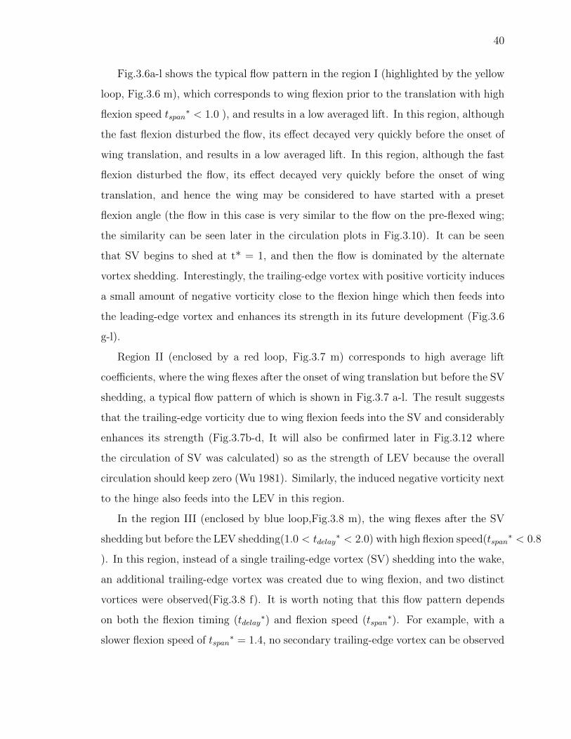
Fig.3.6a-l shows the typical flow pattern in the region I (highlighted by the yellow

loop, Fig.3.6 m), which corresponds to wing flexion prior to the translation with high

flexion speed tspan∗ < 1.0 ), and results in a low averaged lift. In this region, although

the fast flexion disturbed the flow, its effect decayed very quickly before the onset of

wing translation, and results in a low averaged lift. In this region, although the fast

flexion disturbed the flow, its effect decayed very quickly before the onset of wing

translation, and hence the wing may be considered to have started with a preset

flexion angle (the flow in this case is very similar to the flow on the pre-flexed wing;

the similarity can be seen later in the circulation plots in Fig.3.10). It can be seen

that SV begins to shed at t* = 1, and then the flow is dominated by the alternate

vortex shedding. Interestingly, the trailing-edge vortex with positive vorticity induces

a small amount of negative vorticity close to the flexion hinge which then feeds into

the leading-edge vortex and enhances its strength in its future development (Fig.3.6

g-l).

Region II (enclosed by a red loop, Fig.3.7 m) corresponds to high average lift

coefficients, where the wing flexes after the onset of wing translation but before the SV

shedding, a typical flow pattern of which is shown in Fig.3.7 a-l. The result suggests

that the trailing-edge vorticity due to wing flexion feeds into the SV and considerably

enhances its strength (Fig.3.7b-d, It will also be confirmed later in Fig.3.12 where

the circulation of SV was calculated) so as the strength of LEV because the overall

circulation should keep zero (Wu 1981). Similarly, the induced negative vorticity next

to the hinge also feeds into the LEV in this region.

In the region III (enclosed by blue loop,Fig.3.8 m), the wing flexes after the SV

shedding but before the LEV shedding(1.0 < tdelay∗ < 2.0) with high flexion speed(tspan

∗ < 0.8

). In this region, instead of a single trailing-edge vortex (SV) shedding into the wake,

an additional trailing-edge vortex was created due to wing flexion, and two distinct

vortices were observed(Fig.3.8 f). It is worth noting that this flow pattern depends

on both the flexion timing (tdelay∗) and flexion speed (tspan

∗). For example, with a

slower flexion speed of tspan∗ = 1.4, no secondary trailing-edge vortex can be observed

41

Figure 3.7: A typical flow in region II at tdelay∗ = 0.4 and tspan

∗ = 0.4 (b) SV wasenhanced by flap deflection and the net force had a significant increase. (h) Inducednegative vorticity was feed into the LEV. (m) Region II with high average lift, high-lighted by red loop.

despite that the flexion timing is in an appropriate range (tdelay∗=1.2). As a result,

the flow pattern with two successive trailing-edge vortices is only restricted in the

limited region III inside the blue loop.

Finally, region IV corresponds to the lowest average lift (highlighted by green loop,

Fig.3.9 m), and its flow pattern is showed in Fig.3.9a-l. In this region, the flap flexes

during or slightly after the LEV shedding, causing simultaneous shedding of the TEV

and LEV (Fig.3.9e-h).As a result, these two vortices with negative and positive vor-

ticity undergo strong interaction with each other. The LEV is therefore substantially

affected and reduces into a large amount of negative vortical flow connected to the

leading edge and unable to shed completely for a long period of time (Fig.3.9i-l; the

vortical flow connects to the leading edge until t*=7.2 while in region III the vortical

flow connects to the leading edge until t*=4.4). Furthermore, the formation of next

42

Figure 3.8: A typical flow in region III at tdelay∗ = 1.4and tdelay

∗ = 0.8 (d) AnotherTEV was created by deflection beside SV. (j) Induced negative vorticity feeds intoLEV.

LEV is significantly affected and no considerable LEV is produced on the wing in a

long period of time (t∗ = 4.8 6.4), possibly leading to the low lift in region IV.

To further demonstrate the differences of the flow patterns in those four regions

and confirm the categorized flow patterns, the circulations on all the selected flexion

cases were calculated within a rectangular region surrounding the wing (1.4C × 1.6C

in Fig.3.1 (c)) (the calculated region was large enough to cover all the major flow

features close to the wing). We also calculated the circulation values of the flat wing

and pre-flexed wing as the references. These results are summarized in Fig.3.10

As expected, the circulation plots exhibit four different types of behavior. In region

I where the flap flexes before the wing starts with high flexion speed (Fig.3.10a), tthe

circulation curves on those four flow measurement points (black circles in yellow loop

in Fig.3.9m) show very little difference and overlap with the circulation on the pre-

43

Figure 3.9: A typical flow in region IV at tdelay∗ = 2.4 and tspan

∗ = 0.4 (e) TEVcreated by deflection interacted with LEV pronouncedly. (g-i) LEV shedding wasdisturbed, delaying the generation of next LEV. (m) Region IV with significantlyreduced averaged lift, highlighted by green loop.

flexed wing. This is also consistent with our previous observation that the flow in

region I is similar to the flow on the pre-flexed wing. In Fig.3.10b, the circulations

on the measured points in region II are plotted. In the range of 2 < t∗ < 4, the

flow close to the wing is dominated by intense negative vortical flow which can be

inferred to be the strong leading-edge vortex due to the shedding of enhanced SVs

in Fig.3.7 (the overall circulation of the entire flow is zero (Wu 1981)). Fig.3.10c

shows the circulation curves in region III where the flexion occurs between the SV

and LEV shedding. The circulation in this region experiences a secondary drop in

the range of 2 < t∗ < 4 due to the shedding of second TEV (see Fig.3.8). Finally,

Fig.3.10d presents the circulation curves in the region IV. Here, the overlapped region

of circulation curves between the flexed and flat wing cases extends, and the secondary

44

Figure 3.10: Circulation versus normalized time. Circulation curves in the sameregion have similar behavior. (a) Circulation curves in region I overlap with eachother and are closed to the circulation on the pre-deflected wing (black dash curve).(b) Circulation curves in region II have pronounced negative circulation in the rangeof 2 < t∗ < 4. (c) Circulation curves in region III have abrupt drops in the rangeof 2 < t∗ < 4. (d) Circulation curves in region IV experience mild increase over4 < t∗ < 6 and limited decrease over 6 < t∗ < 7.

circulation drop in region III is not observed in region IV. Instead, owing to the strong

interaction between the TEV and LEV (Fig.3.9), circulation mildly increases in the

range of 4 < t∗ < 6 and decreases in the range of 6 < t∗ < 7. In particular, for the

case of tdelay∗ = 2.0 tspan

∗ = 0.4 (the blue curve in Fig.3.10d) where the flexion occurs

close to the LEV shedding, the circulation has the slowest increase with no decrease

observed afterward. In summary, the comparison of the circulations from the flow

measurement further confirms the categorization of the four types of flow patterns.

45

3.4.4 Vortex strength and lift peak

In the beginning of this section, the flow on the flat wing was analyzed by cal-

culating the circulation magnitude of LEV and TEV/SV to determine the timing

of vortex shedding. Here, to investigate the wing flexion effect on the vortices, the

same method of circulation calculation was applied to study the behavior of LEV

and TEV/SV under different wing flexion timings. Fig.3.11a and b give the plots of

circulation magnitude of the LEV and its corresponding shedded free vortex on the

selected cases with the fastest flexion speed but different flexion timings. As com-

pared to the flat wing, wing flexion enhances the LEV if wing flexion happens before

the SV shedding (tdelay∗ < 1.0, Fig.3.11a )However, if the wing flexion happens after

the SV shedding or during the LEV shedding (tdelay∗ > 1.0, Fig.3.11b ), the strength

of LEV and its corresponding free vortex is greatly disturbed and weakened. The

circulation magnitude of the TEV/SV is plotted in Fig.3.11c and d. Compared to

the circulation of LEV, the circulation of TEV/SV is more sensitive to the flexion

timing change. In general, wing flexion cannot affect SV if SV has already shed from

the wing(tdelay∗ > 1.0, Fig.3.11 d) and the circulation of SV is close to the circula-

tion of SV on the flat wing (black curve). In Fig.3.11 c,when 0 < tdelay∗ < 1.0, the

circulations of the SVs have the largest values. Especially, when tdelay∗ = 0.4 , the

SV strength is maximized as the vorticity due to flexion is able to completely feed

into the starting vortex and the highest lift force was observed in the same region. In

fact, correlation between the lift production and starting vortex shedding has been

previously pointed out by Wagner (1925). Here in Fig.3.12, the relation between the

SV strength and lift force is explored by calculating the normalized circulation of SVs

and comparing them with the maximum lift coefficient in the range of −2 < t∗ < 1

(where the SV shedding takes effect) on the selected cases with the maximum flexion

speed but varying flexion timings (−0.8 < tdelay∗ < 2.8 ;tspan

∗ = 0.4). The circulation

of SVs was calculated at t∗ = 1.8 where the wing has translated for 1.44 chord length

and the SVs have already completely shed from the wing. Finally, the calculated

46

circulation value is normalized by the circulation of SV on the flat wing at t∗ = 1.8

. The results indicate that the circulation of the starting vortex (black curve) and

the maximum lift coefficient (red curve) have strong correlation as they varying with

the flexion timing. Both the starting vortex circulation and lift peak reached high

values in the range of 0 < tdelay∗ < 0.4.The lift peak reached its maximum of 5.7 at

tdelay∗ = 0.4 when the SV is the strongest which is reasonable because a strong SV

leads to a strong negative vortical flow around the wing to keep a zero circulation on

the entire flow and therefore might introduce a strong circulatory lift force. When

tdelay∗ > 1.0 , the vorticity due to flexion lags behind the SV, and the normalized

circulation drops to about 1 (the strength of SV in the flat wing), while the lift peak

remains unaffected by the flexion and staying around 2.9 (At tdelay∗ = 1.0, the nor-

malized circulation of SV drops sharply to about 0.5. This is because the trailing

edge vortex due to wing flexion and SV are so close, thereby introducing a strong

interaction between two vortices and finally reducing the strength of SV).

Nonetheless, here we only discussed the lift augmentation due to SV shedding.

In fact, in addition to the SV, the added mass effect and other flow feature (like

LEV) would also affect the lift generation (Xia and Mohseni 2013). At a low angle of

attack of 15o, Pitt-Ford and Babinsky (2013) studied a translating flat plate which

accelerated from the rest by using potential flow theory with the trajectories and

strength of vortices measured through PIV as inputs. It was found that the bound

circulation derived from Kelvins circulation theorem provides the best match between

modeling and flow measurements during the onset of wing translation. The lift force

was finally estimated from superimposing Wagner lift and the non-circulatory force

and provided a good prediction as comparing with the measured force. However, the

same method cannot be applied to current work where re-attached flow assumption

already failed at high angle of attack. Therefore, to fully understand and explain the

lift generation on the dynamic flexing wings, analysis on the added mass effect as well

as the time resolved overall flow features are needed in the future work.

47

Figure 3.11: Circulation magnitude of vortices on the deflected wings with the highestflexion speed (tspan

∗ = 0.4) but different flexion timings (−1 < tdelay∗ < 2.8)) versus

normalized time. (a), (c) Circulation magnitude of LEVs/its corresponding free vor-tices and TEVs/SVs when wing flexion happens before SV shedding (b), (d) Circu-lation magnitude of vortices when wing flexion happens after SV shedding

3.5 Concluding remarks

In this paper, the effects of timing and speed of active wing flexion were studied

systematically using force and DPIV measurements. The results show that significant

improvement on force performance can be achieved by a proper design of wing flexion

kinematics relative to the vortex shedding events. In particular, when the wing flexes

slightly before the SV shedding with relatively fast speed, the wing produces the

maximum lift. However, if the wing flexes during or slightly after the LEV shedding,

the lift is substantially reduced and close to that of the flat wing.

It is also shown that by flexing the wing within a certain range of timing at

moderate speed, the vortex shedding on the wing changes dramatically and leads to

48

Figure 3.12: Comparison between starting vortex strength (Normalized by circulationof SV in flat wing) and its corresponding maximum lift coefficient (in the range of−2 < t∗ < 1) for the cases with highest deflection speed (tspan

∗ = 0.4) but differentdeflection timings (−1 < tdelay

∗ < 2.8).

four different patterns which can be directly related to four regions in the average

lift contour plot (Fig.3.12). First, when the wing flexes before SV shedding, SV is

enhanced by the flexion and a large lift force is observed. Especially, the highest

instantaneous lift is produced when the strength of SV reaches the highest value.

Second, when the wing flexes between the shedding of SV and LEV, a second TEV

is shed in addition to the SV and a moderate average lift is observed. Third, when

the wing flexes during or slightly after LEV shedding, it affects the shedding of LEV

and delays its development, resulting in a low average lift due to the reduced LEV

strength. Fourth, when the wing flexes before the onset of translation at a rapid rate,

a low average lift is observed as the force and flow structures are similar to those

of the pre-flexed wing.Johansson et al. 2008 studied Pallas long-tongued bats in a

wind tunnel under different free stream velocities. Strikingly, Johansson observed a

distinctive vortex pattern in the wake of Pallas long-tongued bats flying in a wind

tunnel, which contained two consecutive TEVs at a low free stream velocity of 2

m/s. In the current study, the same flow phenomenon is found in the region III

(Fig.3.13) where both relative high lift (around 1.5) and liftdrag ratio (around 0.7)

49

Figure 3.13: A summary of active flexion effects on the flow and lift force. (a) Flowon non-deflected flat wing is simply dominated by a starting vortex in the beginningand alternative vortices shedding afterward. (b) By adjust the active flexion timingrespected to the timings of vortices shedding (with moderate flexion speed) four typesof flow pattern can be produced (c) Four average lift regions can be closely related tothe four different flow patterns.

can be achieved, implying the slow flying bat might have optimized lift performance

and efficiency by producing a two consecutive TEVs structure in its wake.

To extend our results to real flapping-wing case, the pronounced wingwake in-

teraction during the stroke reversal (Lua et al. 2011) must be taken into account

along with the effect of varying angles of attack throughout the stroke. Furthermore,

in 3D flapping wings, because the tip and root vortices may play a critical role in

defining the flow structure (Cheng et al 2014; Liu et al 2013), the study of active

wing morphing may do well to consider both the 3D and unsteady effects.

50

4. CONVENTIONAL FLOW VISUALIZATIONS ON MECHANICAL FLAPPERS

4.1 An Application of Smoke Wire Visualization on a Hovering Insect

Wing

Published in Journal of Visualization 2013 (First Author: Yun Liu)

4.1.1 Introduction

Insects are able to achieve a highly stable but maneuverable flight due to their

distinct form of locomotion (Fry et al. 2003; Hedrick et al. 2009). They flap their

wings back and forth at large angle of attack and create augmented lift. In recent

decades, the smoke wire visualization was wildly used in studying the aerodynamics

of insect flight (Ellington et al 1996; Willmott et al. 1997; Nguyen et al. 2009),

as it provides direct and qualitative flow information around the insects and flapper

models. Conventionally, the smoke wire visualization is used in wind tunnels which

provide uniform and low turbulent free streams. Under this restriction, all the pre-

vious experiments of smoke wire visualization on flapping wings were performed in

wind tunnels with nonzero free stream velocity which however could not provide an

ideal hovering flight condition. In this paper we introduce and experiment a new

smoke visualization technique on hovering insect wings.

4.1.2 Experimental Method

Hovering insects and hummingbirds create significant downwash flow (Rayner

1979); therefore, by placing the smoke wire close to the leading edge of the wing,

we expect the downwash to drag the smoke particles into the wake and then visualize

the flow. Based on this method, we tested a pair of Cicada wings driven by a robotic

51

insect model using four-bar mechanism (Fig. 1) (details see Hu et al. 2011). In the

experiment, the smoke was generated using paraffin oil heated along a stainless steel

wire with 0.25 mm diameter. The steel wire was installed parallel to and 5 mm away

from the vertical stroke plane of the flapping wing (Fig. 2). Both the steel wire and

the robotic model were installed on an aluminum alloy frame contained in a clear

plexglass box, which prevented any air disturbances from the environment. A high-

speed camera (Fastec Trouble Shooter, FASTEC IMAGING CORPORATION, San

Diego, CA, USA) was used to record the smoke pattern at 1,000 frame/s, which was

illuminated using a LED work Lamp. To increase the image resolution, the smoke

pattern of a single wing (instead of the wing pair) was recorded. The experiments

were performed at three different flapping frequencies: 5 Hz, 10 Hz, and 16 Hz.

Figure 4.1: Flapper with cicada wings Figure 4.2: The experimental setup

4.1.3 Results and Discussion

Fig.4.3 shows the smoke visualization results for the flapping frequency at 5Hz, and

results for other frequencies are shown in the supplementary materials. In Fig.4.3a,

six frames for an upstroke (0-100ms) are shown, and three frames at 0, 40 and 100ms

are shown in Fig.4.3b-d with more details. During the down-stroke, a large downwash

accompanied by a strong vortex at wing tip and a minor vortex at wing base were

observed (Fig.4.3b). At the beginning of the upstroke, after the wing quickly rotating,

52

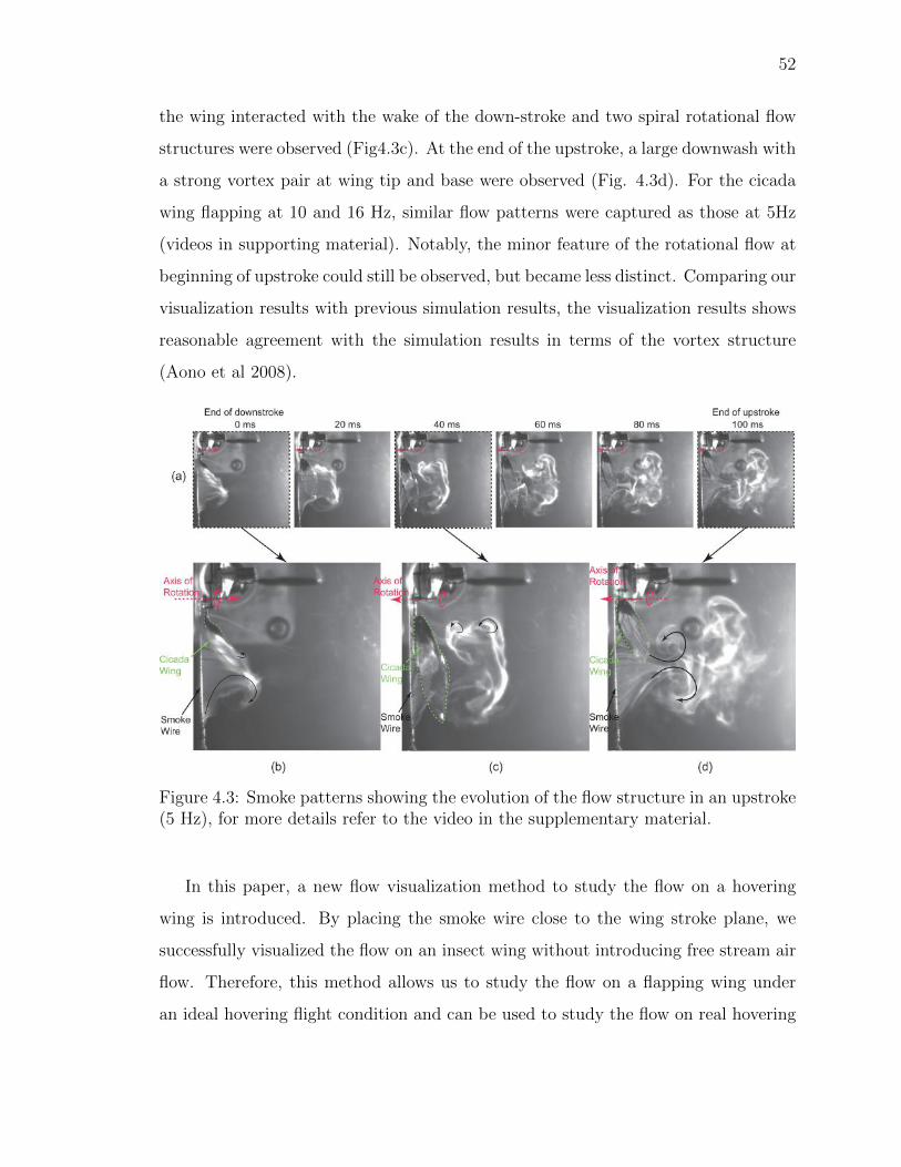
the wing interacted with the wake of the down-stroke and two spiral rotational flow

structures were observed (Fig4.3c). At the end of the upstroke, a large downwash with

a strong vortex pair at wing tip and base were observed (Fig. 4.3d). For the cicada

wing flapping at 10 and 16 Hz, similar flow patterns were captured as those at 5Hz

(videos in supporting material). Notably, the minor feature of the rotational flow at

beginning of upstroke could still be observed, but became less distinct. Comparing our

visualization results with previous simulation results, the visualization results shows

reasonable agreement with the simulation results in terms of the vortex structure

(Aono et al 2008).

Figure 4.3: Smoke patterns showing the evolution of the flow structure in an upstroke(5 Hz), for more details refer to the video in the supplementary material.

In this paper, a new flow visualization method to study the flow on a hovering

wing is introduced. By placing the smoke wire close to the wing stroke plane, we

successfully visualized the flow on an insect wing without introducing free stream air

flow. Therefore, this method allows us to study the flow on a flapping wing under

an ideal hovering flight condition and can be used to study the flow on real hovering

53

animals. However, this method of flow visualization can only capture the flow passed

around the smoke wire not the entire three-dimensional flow. In the next section, dye

visualization method will be explored to test its capacity in the study of the entire

complex flow in flapping wings.

54

4.2 Dye Visualization on a Mechanical Flapping Wing

4.2.1 Introduction

The flow pattern from smoke visualization actually presents the streak-lines which

are quite different from the stream-lines in a highly unsteady flow (Smits and Lim

2000). Additionally, the smoke visualizations can only visualize the flow passed

around the smoke wires or the places where the smoke was released. Therefore,

the smoke visualization, as a common and conventional method in studying insect

flight, is very restricted and can only capture and present limited flow information

about the flapping wings. On the other hand, dye visualization, another common flow

visualization method, is capable of visualizing the overall unsteady three-dimensional

flow and has been succesfully demonstrated in several cases. For example, the dye vi-

sualization was successfully implemented on a pitching plate, visualizing a well linked

three-dimensional vortex skeleton(Buchholz et al 2008). The fluorescent dye was also

applied on a falling disk with the three-dimensional structures of tip vortices nicely

visualized and captured (Lee et al 2013).

4.2.2 Experimental Method

A dynamic scaled flapper was designed to flap back and forth with two degrees

of freedom (rotation and stroke) in a water tank at a frequency of 1/4 Hz. Wing

kinematics was accurately controlled using a PID feedback control loop in simulink

MATLAB with wing rotation and stroke angle in two sinusoidal functions. Before

putting the wing into the tank, fluorescence dye was brushed on the wing surfaces.

Once the wing was emerged in the water, the flapper started to flap. The wing

platform is based on the fruit fly wing with a length of 40 mm. To let the fluorescent

dye well attached to the wing surfaces, the wing was made from a plate of wooden

balsa so that the fluorescence dye can soaked into the material. Finally the evolution

55

of flow structure was recorded by using a digital camera (Nikon) at a frame rate of

60 fps.

4.2.3 Results and Discussion

Dye shed DuringWing entering the water

Vortex ring

LEV connects to Tip vortex

Shed vortex ring

Tip Vortex Root Vortex

Tip Vortex

Root Vortex

Shed vortex ring

(a)t = -2/20 T

(e)t = 2/20 T

(i)t = 10/20 T

(b)t =-1/20 T

(f)t = 4/20 T

(j)t = 12/20 T

(c)t = 0/20 T

(g)t = 6/20 T

(k)t = 14/20 T

(d)t = 1/20 T

(h)t = 8/20 T

(l)t = 16/20 T

Figure 4.4: Dye visualizaiton results on a mechanical flapper.

Fig.4.4, shows a sequence of dye visualization results on the balsa wood wing in

the very first stroke. Fig.4.4a-c present the vortical flow created during the onset of

wing flapping. A clear vortex loop was created with part of it attached onto the wing

surface as a leading edge vortex. In Fig.4.4d-h, the vortial flow in the first half stroke

56

is presented. During this half stroke, the vortex loop produced during onset was no

longer attached onto the wing and shed into the wake while significant root and tip

vortices were created with their ends connecting to the shed vortex loop. The leading

edge vortex, growing from the root to tip, tilted significant near the tip and connected

to the tip vortex. Fig.4.4i-l, present vortical flow in the second half stroke. During the

stroke reversal, no vortex loop can be observed. Instead, strong tip and root vortices

were created in the wake. Notably, the tip and root vortices move toward each other

as they convecting downward which has been also observed in the Chapter 2, showing

the tip and root vortices are converging in the two-layer structure.

Here, in this section, dye visualization was implemented on a mechanical flapping

wing. The dye brushed on the wing surfaces can nicely track the major flow feature

like leading edge vortex, tip vortex and root vortex. Under current experimental

setup and experimental conditions, the visualization result indicates the wake flow in

the flapping wing is dominated by the tip and root vortices with leading edge vortex

attached on the wing surface though out the flapping cycles except the stroke rever-

sals. Compared to the volumetric flow measurement in the Chapter 2,however,vortex

ring structure is not captured in this dye visualization study which might be casused

by the difference of the wing kinematics.

Although the V3V flow measurement and dye visualization in Chapter 2 and 4

depict detialed vortical flow structures on flapping wings, it is clearly questionable to

refer our results to real flying insects, considering their complex wing morphologies.

In next chapter, a substantial new study will be carried out on a freely flying insect

to study the authentic complex flow in flapping wings.

57

5. INSECTS FLY ON LADDERS OF VORTICES

Submitted (First Author: Yun Liu)

5.1 Chapter Abstract

To date, a comprehensive understanding of the complex flow topology generated

by freely flying insects has eluded the scientific community due in part to the inabil-

ity to adequately study the unsteady three-dimensional flow structure in a natural

setting (Srygley et al 2002,Henningsson et al 2015, Johansson et al 2013). In the

absence, researchers have primarily relied upon either two-dimensional conventional

flow visualizations/measurements on tethered insects or dynamically scaled experi-

ments utilizing robotic flappers fitted with scaled insect wings undergoing simplified

flapping motion (Ellington et al 1996,Birch and Dickinson 2003, Bomphrey 2006,Pick

and Lehmann 2009, Mountcastle and Daniel 2009,Lua et al 2010). To overcome the

limitations of these studies, a new method of flow visualization is developed and suc-

cessfully implemented on freely flying hawkmoth Manduca sexta. We discovered a

linked ladder like vortex structure under each wing on freely flying Manduca. This

linked ladder structure of vortices is formed by the vortex loop produced in the down-

stroke joined by the tip and root vortices in the upstroke. After every stroke reversal,

the newly formed vortex structure is linked to the previous vortex structure created

in the last half stroke, thus forming a ladder of vortices under each wing. Previous

experimental flow observations on fish and pitching plates have also revealed similar

linked chains of vortices (Drucker and Lauder 1999, Flammang et al 2011, Buchholz et

al 2008), suggesting a commonality of linked vortex structure among different forms

of animal locomotion.

58

5.2 Results and Discussion

The complex flow topology of flapping wings, revealed through smoke visualization

techniques conducted on insects and robotic flappers, established the prominence of

a stably attached LEV responsible for lift augmentation in flapping wings (Van den

berg and Ellington 1997, Ellington et al 1996), differentiating this unique form of

animal locomotion from conventional fixed wing aerodynamics. Further character-

ized by scaled tank experiments with robotic flappers, quantitative force data was

correlated to models of the quasi-steady aerodynamic mechanisms formulated from

detailed experimental observations(Dickinson et al 1999). Computational Fluid Dy-

namics (CFD) simulations using simplified flapping wing motion, on the other hand,

have provided an abundance of flow and force data, supporting empirical results and

providing further intuition (Liu et al 1998). The results of these fundamental studies,

in addition to several others (Weis-Fogh 1973,Maxworthy 1979, Dudley and Ellington

1990, Fry et al 2003, Sun and Tang 2002, Lentink and Dickinson 2009, Wang 2005),

form the foundation of our current understandings on the aerodynamics of insect

flight.

In the establishment of these findings, however, researchers have relied primarily

upon experiments on either tethered insects or robotic flappers but rarely on freely

flying insects. Moreover, experimental observations of the local and extended flow

field on flying animals have been limited by the applications of traditional flow visu-

alization/measurement techniques. For instance, smoke wire visualization techniques

used on tethered or freely flying insects in wind tunnels necessitate a non-negligible

relative flow velocity (larger than 0.4m/s) (Srygley et al 2002, Ellington et al 1996,

Bomphrey et al 2009, Thomas et al 2004), thus precluding the study of hovering

flight. Smoke plume visualization on a hovering hummingbird was used to recon-

struct portions of three-dimensional structure in the downwash without continuously

capturing the details of vortices (Pournazeri et al 2012). These visualization meth-

ods, after all, depict patterns of streaklines leaving the vortical structures to be later

59

interpreted from these patterns (Smits and Lim 2000). Particle image velocimetry

(PIV), on the other hand, has been used extensively in the study of insect flight

(Johansson et al 2013,Birch and Dickinson 2001, Bomphrey 2006, Pick and Lehmann

2009, Mountcastle and Daniel 2009), with recent applications of tomographic PIV

providing measurements of the three-dimensional flow structure in the far field wake

of a tethered locust (Henningsson et al 2015). However, these quantitative studies

have either focused on the near-field flow features on two-dimensional planes or far

field three-dimensional flow features in the wake region away from the wings. Thus a

detailed overview of three-dimensional vortex structure, in both near- and far field,

has never been fully captured on a freely flying insect.

The present work overcomes the limitations associated with these traditional flow

visualization/measurement methods through the use of a density gradient medium

(isopropyl alcohol) applied to the surfaces of insect wings and the use of high speed

Schlieren photography. For the first time, the overall vortex structure and its develop-

ment on freely flying hawkmoth Manduca sexta is directly visualized experimentally,

revealing a linked ladder structure of vortices under each wing.

Utilizing this new method, images of distinct vortex structures were obtained on a

near hovering Manduca and an ascending Manduca. Fig 5.1 and 5.2 present the flow

structure on a near hovering Manduca with an average flying speed of 0.3 m/s. Fig.

1 shows the images of vortex structure in the down-stroke. A combined structure

of starting vortex and stopping vortex was observed on each wing in the beginning

of down-stroke right after wing pronation (Fig 5.1 a). Then very quickly, on each

wing, distinct tip vortices were generated by both the fore- and hind-wing (Fig 5.1

a). Meanwhile, a stable leading edge vortex was created with one end connecting to

the fore-wing tip vortex. However, we found no evidence of a continuous leading edge

vortex crossing over the thorax which was observed in the previous flow visualiza-

tion/measurement studies on tethered Manduca in the wind tunnel6; instead, a cone

shaped leading edge vortex was observed (Fig 5.1 c) on each wing. As a result, an

open vortex loop (or horseshoe-shaped vortex (Liu et al 1998, Zheng et al 2013) is cre-

60

Figure 5.1: Vortex structures captured in the down-stroke on a near-hovering malehawkmoth (mass 1.26 g) with an average flying speed of 0.3 m/s (See SupplementaryVideo 1). a. A combined structure of starting/stopping vortex after wing pronation.b. Tip vortices are created from not only tips of fore-wings but also tips of hind-wings. c. An attached cone shaped leading edge vortex before wing supination.d. Eventually, the down-stroke of each wing creates an open vortex loop (horseshoevortex loop), connecting the leading edge vortex, tip vortex, starting/stopping vortex,and root vortex.

ated on each wing, connecting the leading edge vortex, tip vortex, starting/stopping

vortex, and root vortex (Fig 5.1 d). Video of the vortex structure in down-stroke can

be found in the supplementary video file Fig.1.avi. This open vortex loop structure

on Manduca has been previously observed in experimental and numerical studies on

Manduca models (Van den berg and Ellington 1997, Liu et al 1998,Zheng et al 2013).

Having never been observed on freely flying Manduca directly, the observance of the

open vortex structure presented in this work thus serves as the first confirmation of

61

these studies. Furthermore, unique to previous experimental and numerical studies

on Manduca, the existence of a secondary hind-wing tip vortex as revealed by this

technique presents a more complete depiction of the open vortex loop structure gen-

erated by flapping wings. At the end of the down-stroke, during the supination (Fig

5.1c), the cone shaped leading edge vortex, under a significant deformation due to

the rapid wing twisting, can be clearly seen. Subsequently, the leading edge vortex is

then shed into the wake along with the other vortices created during the down-stroke,

forming a closed vortex loop.

The vortex structure during the upstroke is shown in Fig 5.2. After wing supina-

tion, a closed vortex loop was shed into the wake from each wing while two strong tip

vortices were created from the tips of fore- and hind-wings with ends connecting to

the previously shed vortex loop (Fig 5.2 c). Concurrently, a root vortex was created,

also connecting to the shed vortex loop. However, unlike the flow structure captured

in the down-stroke, we found no evidence of a strong attached leading edge vortex

during the up-stroke. This is consistent with results from smoke visualization studies

and CFD simulations on a hovering Manduca model (Van den berg and Ellington

1997, Zheng et al 2013), and is indicative of a lack of vortex loop formation during

the up-stroke. Therefore, after one complete wing beat cycle, the resulting vortex

structure created under each wing consists of a vortex loop in the far wake, two tip

vortices and a root vortex in the near field.

Fig.5.3a-b show the vortex structure on an ascending Manduca with an average

speed of 0.7 m/s. Similar to vortex structures in Fig.5.1 and 5.2, an open vortex

loop is first created on each wing during the down-stroke and shed after supination

(Fig.5.3a). In the up-stroke, two strong tip vortices were created from the tips of fore-

and hind-wings and linked to the previously shed vortex loop (Fig.5.3b). Interestingly,

vortex structure visualized on the ascending Manduca illustrated a more pronounced

linked ladder like structure which not only connects the vortex structures between

down- and up-stroke but also connects the vortex structures between each wing beat

cycle. In the near hovering flight case, evidence of the linked structure can be also

62

Figure 5.2: Vortex structures captured in the up-stroke on the near hovering hawk-moth (See Supplementary Video 2). a. The vortex loop created in down-strokesheds into the wake. b-c Long, stretched tip vortices from the tips of fore-wings andhind-wings are created and connected to the just shed vortex loops. d. Finally, theup-stroke of each wing creates long, stretched tip and root vortices, connecting theshed vortex loop to the wing.

found. Fig.5.3c depicts the linkage formation between the vortex structure in a wing

beat (up-stroke) to the vortex structure in the next wing beat (down-stroke) in the

near hovering case. During wing pronation, the tip/root vortices from the up-stroke

shed from the wings and then connect to the stopping/starting vortices, formed in

the beginning of the down-stroke, thereby connecting the vortex structures between

each wing beat. Consequently, our direct flow visualization results reveal a well

63

Figure 5.3: Vortex structures from consecutive wing beat cycles are well linked. a-b.The vortex structure capured on an ascending male hawkmoth(mass 0.93 g) withan average flying speed of 0.7m/s (left and right columns show the flow structurefilmed from front and side views). a. On the ascending hawkmoth, a vortex loopis created on each wing in the down-stroke and the vortex loop is connected to thevortex structure creaed from the last up-stroke.b.In the up-stroke, stretched hind-andfore-wing tip vortices as well as root vortex are created on each wing,connecting to thevortex loop from the down-stroke.c.Between consecutive wing beat cycles, a linkedstructure is also observed on the near hovering hawkmoth. Tip vortices from theup-stroke shed from the wings and connect to the starting/stopping vortices, therebyconnecitng the vortex structures between each wing beat cycle. Left image shows theoriginal image of the strucutre and right image shows notated vortex structure.

linked vortex structure on freely flying Manduca. Especially in the ascending case,

the Manduca creates a ladder of vortices under each wing. However, due to flow

dissipation and instabilities, the entirety of the ladder-like structure underneath the

wing could not be seen. Instead, only the linked structure within two wing beats is

64

visible, with the remaining structure dissipated into the wake. Ignoring these effects

and hind-wing tip vortex, a simplified linked vortex model is presented in Fig.5. 4.

Figure 5.4: Vortex ladder under an ascending hawkmoth. a. In the down-stroke,a vortex loop is created and linked to the other vortex loops through tip and rootvortices formed from up-strokes, forming a ladder of vortices under each wing. b. Inthe up-stroke, stretched tip and root vortices are created on each wing connecting thejust shed vortex loop to the wing.

The linked ladder structure of vortices presented may not be unique to Manduca,

but rather may be a common feature of multiple forms of animal locomotion. Both

two-dimensional PIV measurements and volumetric flow measurements have revealed

linked vortex rings or chains of vortex rings on freely swimming fish (Drucker and

Lauder 1999, Flammang et al 2011). Smoke visualization on hovering hummingbirds

illustrated a bilateral vertically connected vortex ladder structure under the pair wings

(Pournazeri et al 2013). Utilizing a state of the art flow visualization method, a chain

65

of linked vortex rings was also found to form the wake of a pitching plate undergoing

periodic motion similar to that of flying and swimming animal locomotion (Buchholz

et al 2008); The formation of this chain of linked vortex rings was associated with

the pitching plate at the highest thrust efficiency, while the wake divides into two

separate trains of vortical structure at low thrust efficiency. Similarities between the

linked vortex structure found on pitching plate and the vortex ladder observed on

each Manduca wing suggests a possible connection between the formation of single

chain vortex ladder structures and optimal thrust efficiency in freely flying Manduca.

Clearly, the mechanics of unsteady force generation and unsteady three-dimensional

wake structure must be correlated. Therefore, from a more complete depiction of the

wake topology on freely flying insects and its evolution, the complexities of flying

insect aerodynamics and associated performance metrics (like efficiency) can be more

accurately modeled and assessed.

The flow topology of flying Manduca has served as a classic study case for flapping

wing locomotion, having been the subject of scientific research for over two decades.

However, due to the limitations of traditional flow visualization techniques, the overall

vortex structure on a freely flying Manduca has never been fully captured until now.

Utilizing a new method of flow visualization on flying insects, this work reveals a

linked ladder structure of vortices on each wing of the freely flying Manduca, resulting

from the formation of a vortex loop created during the down-stroke (see Fig.4a)

and long, stretched tip and root vortices created during the up-stroke connecting

the shed vortex loop to the wing (see Fig.4b). During wing pronation, the tip and

root vortices in up-stroke shed from the wing and connect to the stopping/starting

vortices in the down-stroke, thereby forming a ladder of vortices. In addition to

this topological depiction of the wake, several clarifying remarks about the observed

vortical structure of freely flying Manduca can be made. First, the wing pair of flying

Manduca clearly create a bilateral vortex structure without formation of a single

vortex ring in the down-stroke where by the LEV is continuous over the thorax6.

Second, in the up-stroke, no evidence of a strong attached LEV was found, suggesting

66

the existence of a weak or even no formation of a LEV on freely flying Manduca in

up-stroke27 . Lastly, applications of this new method of flow visualization are not

limited to the current study and could also be used in the study of other flying animals

ranging from hummingbirds (Trochilidae) and butterflies (Lepidoptera) to smaller

insects such as flies (Diptera). By providing sufficient time resolved three-dimensional

information about the complex flow structure, results from this technique could be

used as validation for existing flow measurements and CFD simulation results.

5.3 Method

Male Manduca sexta adults were obtained from the Purdue University Entomol-

ogy department. A high speed Schlieren photography system was implemented to

visualize the unsteady three-dimensional vortical flow on freely flying Manduca. This

system consists of two single mirror, double-pass, Schlieren setups with two high speed

cameras (Mini UX100, Photron), filming from two orthogonal views. In each Schlieren

system, a white LED light was projected through a 1 mm pin hole onto a 10-inch di-

ameter optical spherical mirror (Edmond optics). A portion of the reflected light was

then redirected towards the high speed camera using a 50/50 (reflection/transmission

ratio, Edmond optics) beam-splitter for capture. At the focal point of the reflected

light, a razor blade was used as the knife-edge producing the Schlieren images (See

Fig.5.5).

To trace the vortical flow produced by the flapping Manduca wings, warm iso-

propyl alcohol (91% Isopropyl Alcohol heated to 38oC) was brushed onto the surface

of both wings in the beginning of each test. The Manduca was then released to fly

freely in the flow observation region. Upon wing acceleration and rotation, airflow

over the wing surface increases vaporization of the alcohol, drawing it into the vor-

tex sheet/vortices created from the wing surface. The Schmidt number of vaporized

median is estimated to be on the order of one, taking the diffusion coefficient of iso-

propyl alcohol in air to be 0.1011 cm2/s. Since the diffusion rates of vorticity and

67

Figure 5.5: Experimental Setup

the visualization median are comparable, formations depicted by the alcohol vapor

will accurately capture the vortical flow structures in the absence of strong vortex

stretching.26 Through our high speed Schlieren photography system, the unsteady

three-dimensional vortex structure was visualized and recorded by two high speed

cameras at 1000 frames per second from two orthogonal views. Similar methods of

flow visualization have also been used to study the vortical flow development around

moving objects (Veldhuis et al 2005, Pierce 1961). In total, thirty tests were con-

ducted and results from the two most illustrative tests were presented in this paper.

68

To enhance images of the complex vortex structure on the Manduca, the brightness

and contrast of the images were adjusted accordingly using Adobe Photoshop CS6.

The moths average translating speed was extracted by tracking an eye of the Manduca

using DLTdv5 (Hedrick 2008) .

69

6. SUMMARY

Insect flight is essentially a complex system that requires multidisciplinary efforts

from different perspectives. This thesis focuses on the aerodynamics of insect flight

from a fluid mechanics point of view, studying three highly coupled features in the

aerodynamics of insect flight: unsteadiness, three-dimensional effect and wing mor-

phing.

The V3V system (or Defocusing-DPIV method) lends us a great opportunity to

study the coupling between unsteadiness and three-dimensional effect. Its ability of

measuring instantaneous three-dimensional velocity field in a volumetric space makes

this method unprecedented in studying complex flow on mechanical flappers, com-

pared with other conventional flow visualization/measurement methods. Utilizing

the V3V system, the entire unsteady three-dimensional flow field on a mechanical

flapper was quantified and visualized, depicting a linked vortex rings structure in the

near-field and two layers of vortical flow in the far-field. Yet, due to the limitations

of the laser and other related equipment, a time resolved flow measurement could

not be achieved. As the resulting aerodynamic force on the flapping wing depends

on the time derivative of the vorticity field(Wu 1981), it is impossible to build a di-

rect correlation between the flow field and the resulting aerodynamic force without

time resolved flow data. Moreover, regardless the aero-elastic issue, the actual flap-

ping wing motion of flying insect is hard to be mimicked on the small one degree

of freedom mechanical flapper only which can fit into the small measurement space

(10cm×14cm×14cm). This issue was later overcome by using a larger two degrees

of freedom mechanical flapper with several measured flow regions patching around

the flapper to obtain the entire flow field (Cheng et al 2014). However, with a much

larger measured space, the time spent on data processing is significantly increased.

70

In the absence of three-dimensional effect, the coupling between unsteadiness and

active wing morphing is investigated on a large aspect-ratio translating wing. In-

terestingly, similar flow phenomenon from previous wind tunnel experiments on bats

was also observed in our study, indicating the effectiveness of our simplified model

in representing the active morphing wing. Our study also reveals the dominate role

of wing deformation timing in the flow and aerodynamic force characteristics. Al-

though a primary correlation between the flow and aerodynamic force characteristics

have been presented, a deeper investigation on the added mass effect and vortex force

should be conducted to determine the role of wing acceleration. Therefore, if pos-

sible, it is necessary to study the active wing morphing effect under different wing

acceleration durations (acceleration duration is fixed at 0.4 second in our study) to

have a better understanding on the coupling of unsteadiness and wing morphing.

Yet, on flying animals, the aerodynamics is essentially the outcome of the com-

plex coupling and interaction of all those three factors. As there is no mechanical

flapper can perfectly simulate the flying animals with all these factors considered,

thus, the optimal way of studying flapping wing aerodynamics is study the flow on

real flying animals. In the meanwhile, considering the limitations of traditional flow

visualization/measurement methods, a new method to of capturing and presenting

the complex flow topology on freely flying animals is in a great demand.

In the beginning, I explored two very typical and traditional flow visualization

methods: smoke and dye visualizations. Particularly, the smoke wire visualization

was implemented by placing the smoke wire close to the flapper to visualize the

downwash flow on a ′hovering wing without introducing any free stream velocity.

Dye visualization was also implemented on a mechanical flapper in a water tank.

Because the dye, released from the wing surface, actually presents the passive scalar

which can depict and follow the formation of vortex structure,it provids a complete

picture about the three-dimensional vortical flow on the flapper. Based on the dye

visualization study and Pierces pioneering flow visualization work with shadowgraph

(Pierce 1961), I proposed and implemented a new method of flow visualization on

71

flying insects,by introducing alcohol vapor on the insect wings to track the formation

and development of three-dimensional vortical flow which can be later seen through

a high speed Schlieren photography system.

Our new method with isopropyl alcohol is able to directly visualize and present the

vortical flow. The diffusion coefficient of isopropyl alcohol in the air is 0.1011cm2/s,

making its Schmidt number on the order of 1 which is the most desired number for

the media to track the vortical flow in the absence of strong vortex stretching (the

Schmidt number for smoke and dye visualization is around 1000. So dye or smoke can

only track the vortex formation in the near wake flow region (Buchholz et al 2008).

This advantage can be explained in the following.

∂ω

∂t= −(V ·∇)ω + (ω·∇)V + ν∇2ω (6.1)

∂S

∂t= −(V ·∇)S +D∇2S (6.2)

Equation 6.1 is the vorticity transport equation and Equation 6.2 is the passive

scalar transport equation. ν in equation 6.1 is the kinematic viscosity, presenting

the speed of momentum diffusivity and D in equation 6.2 is the diffusion coefficient,

presenting the speed of mass diffusivity. Schmidt number is defined as the ratio of

ν to D. With Schmidt number in the order of 1, it means the value of ν is close to

the value of D. Then the equation 6.1 and 6.2 are almost identical expect the vortex

stretching term (ω·∇)V . Therefore, in the absence of strong vortex stretching and

with isopropyl alcohol released from the wing surfaces (the origion of vorticity), the

alcohol can nicely track the formation and evolution of the vortical flow in both near-

and far- field(Smits and Lim 2000). In addition, comparing with the tomographic

PIV, this method has a great advantage of efficiency and simplicity. For example,

to resolve the volumetric flow velocity field in the wake region of a tethered locust,

nearly 100 days were taken to process all the images captured from eight high speed

cameras (Henningsson et al 2015).

72

Figure 6.1: Secondary hind-wing tip vortex on a butterfly(images were shot in asequence from a to d)

Clearly, our method of flow visualization has a great potential in studying the

complex flow of flying animals and it was already tested on different insects. For

example, Fig.6.1 shows the visualization results on a flying butterfly. Instead of

introducing isopropyl alcohol on the wing surfaces of the butterfly, the butterfly wings

are hold and warmed by electromagnetic holder and the warm air closed to the wings

is served as the passive scalar to track the vortical flow. Once the butterfly was

released from the electromagnetic holder(not showned in the images), it flapped its

wings and the vortical wake was visualized. Especially, similar to the flow on the

flying hawkmoth, a clear indication of secondary hind-wing tip vortex was observed

,suggesting the commonality of secondary hind-wing tip vortex amongst different

insect speicies. The formation of this secondary tip vortex can be explained based

on Helmholtz’s theorem which suggests the vortex filament cannot end in fluids and

should be in a closed form.

73

Figure 6.2: An explaination of the Secondary Tip vortex. Leading edge vortexstrength is not evenly distributed with vortex filaments shed not evenly, creatinga secondary vortex somewhere from wing root to tip. The red loops indicate thevortex structures created in down-stroke and vortex structure created in up-stroke isin blue

In Fig.6.2, on a flapping wing, the velocity along the the wing span is continuously

growing from wing root to tip, due to the wing rotation. Therefore, the strength of

leading edge vortex should be growing along the wing span in the beginning and

quickly drop to zero at wing tip. Assuming the leading edge vortex is the dominant

spanwise vortical flow (Ellington et al 1996), then to creat a high strength LEV close

to wing tip and low strength LEV close to wing root, mutiple closed vortex loops(with

74

the same strength) should be superimposed unevenly. Thus more vortex filaments

will shed from the wing tip and finally roll up into a strong tip vortex. At wing root

fewer filament will shed and form the root vortex with the strength much less than

the one of tip vortex. The rest vortex filaments, with the same rotating direction of

root vortex but opposite rotating direction of tip vortex, will shed somewhere between

wing root and tip, forming a secondary vortex. On flying hawkmoth and butterfly,

the secondary vortices are all created closed to the tips of hind-wing with the reason

not well understood yet.

Figure 6.3: High speed Schlieren photography on a tethered Wasps

The main difficulty of this flow visualization method, however, is the treatment

to live animals: how to apply the tracking media to their wing membranes and

how to make them to freely fly in the designed region. Espeically, it is even more

challenging to utilize this method on some small insects. Fig.6.3 shows a test of this

flow visualization method on a tethered wasps(The alcohol was only applied on the

right wing). With images enhanced already, it is still hard to see the flow structure

created on the wasps wing. There are basically three reasons that the flow was not

well visualzied. First, small insects like wasps have very high flapping frequency. The

75

alcohol will vaporize very quickly under high flapping frequncy after applying it onto

the wing surfaces. Second, since the insect is quite small, it is very difficult to apply

alcohol to the tiny wing memberane and hard to ensure enough alcohol was applied

on all the wing sufaces. Third, a powerful camera lense is needed for small insects.

In our tests, we used a 50-200 mm zoom lense, clearly not enough for resolving the

flow image on a small insect like wasps. Therefore, to study the flow on small insects,

this method of flow visualization has to be improved and modified accordingly.

Figure 6.4: High speed Schlieren photography on a falling plate

Regardless the limitations of this method of flow visualization on small insects,

this method is indeed a powerful tool in studying the three-dimensional unsteady

flow and can be extended to other contex of studies. Fig.6.4 presents the flow visu-

alization results on a falling plate. However, this method is qualitative after all and

the corresponding results are hard to be quantitatively evaluated and processed. In

the light of advancement on cameras (For example light field camera) and imaging

techniques (holographic imaging), it is possible to improve and upgrade this method

to a quantitative measurement tool in the future.

APPENDIX

76

A. APPENDIX

A.1 Flow Uncertainty

The uncertainty analysis of flow measurement and force measurement in Chapter

3 are addressed here. MATLAB function ′curl′ was used to calculate the vorticity.

In ′curl′, the vorticity was calculated using central finite difference:

ωi,j = (ui,j+1 − ui,j−1yi,j+1 − yi,j−1

− vi+1,j − vi−1,jxi+1,j − xi−1,j

)physicalspace (A.1)

In Equantion A.1 the velocity(u,v) in physical space is actually the velocity on the

image times the calibration factor K and will eventually cancel out in the equation.

Thus, the uncertainty in calibration will not affect the uncertainty on the vorticity

measurement.

ωi,j =K(ui,j+1 − ui,j−1)image

K(yi,j+1 − yi,j−1)image

− K(vi+1,j − vi−1,j)image

K(xi+1,j − xi−1,j)image

= (ui,j+1 − ui,j−1yi,j+1 − yi,j−1

− vi+1,j − vi−1,jxi+1,j − xi−1,j

)image

(A.2)

Since the size of interrogation window is 32 X 32 pixels then yi,j+1 − yi,j−1 =

xi+1,j − xi−1,j = 32 pixels So the uncertainty of vorticity:

δωi,j =1

32δ(ui,j+1 − ui,j−1 − vi+1,j + vi−1,j)image (A.3)

Because the temporal uncertainty is negligible,

δωi,j =1

32∆tδ(dxi,j+1 − dxi,j−1 − dyi+1,j + dyi−1,j)image

=1

32∆t

√(2δ(dx)2 + 2δ(dx)2)image

(A.4)

77

The spatial displacement accuracy for 32X32 interrogation window is + 0.06 pix-

els. So δ(dx)=δ(dy)=0.06 pixels. Thus, δωi,j=0.625 1/s(in the measurement ∆t=6

ms). In addition, there was nuance of the relative motion between the camera and

wing model during the accelerating phase. This relative motion would cause variation

in velocity measurement but will not affect the vorticity measurement because the

small relative motion only introduces a uniform displacement field and calculation of

vorticity will remove this effect. Thus the relative linear translation between cam-

era and wing model will not introduce any uncertainty on vorticity measurement.

Since the maximum measured vorticity is about 25 /s thus the relative uncertainty

of measured vorticity is around 4% .

A.2 Force Uncertainty

The uncertainty of force measurement is derived here and estimated at about 3

%. The aerodynamic drag force was calculated from subtracting the measured force

on drag component FD,measure by the inertia force due to translation FD,T as well as

the inertia force due to deflection on drag direction FD,D.

FD,Aero = FD,Measure − FD,T − FD,D (A.5)

Therefore, the uncertainty of aerodynamic drag force can be calculated by:

δFD,Aero =√δF 2

D,measure + δF 2D,T + δF 2

D,T (A.6)

Here in this study, FD,measure=FY · sin(α)-FX · cos(α) Then

δFD,measure =

√(∂FD,measure

∂FY

δFY )2 + (∂FD,measure

∂FX

δFX)2 + (∂FD,measure

∂αδα)2

=√

(δFY · sin(α))2 + (δFX · −cos(α))2 + (FY · cos(α) + FX · sin(α))2 · δα2

(A.7)

78

Current sensor has an uncertainty of δFX=δFY =0.01 N (retrived from TSI doc-

uments). FX=0.1N; FY =1.0 N(the highest measured force).In our measurement, δα

=1o=0.0175 rad (Protractor was used to measure the AOA). Therefore,

δFD,measure=0.0178. To calculate δFD,D,

δFD,D =√

(δFY · sin(α))2 + (δFX · −cos(α))2 + (FY,D · cos(α) + FX,D · sin(α))2 · δα2

(A.8)

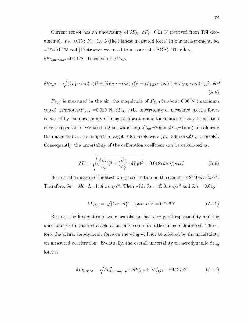
FX,D is measured in the air, the magnitude of FX,D is about 0.06 N (maximum

value) therefore,δFD,D =0.010 N. δFD,T , the uncertainty of measured inertia force,

is caused by the uncertainty of image calibration and kinematics of wing translation

is very repeatable. We used a 2 cm wide target(Lm=20mm;δLm=1mm) to calibrate

the image and on the image the target is 83 pixels wide (Lp=83pixels;δLp=5 pixels).

Consequently, the uncertainty of the calibration coeffcient can be calculated as:

δK =

√(δLm

LP

)2 + (Lm

L2P

· δLP )2 = 0.0187mm/pixel (A.9)

Because the measured hightest wing acceleration on the camera is 2450pixels/s2.

Therefore, δa = δK · L=45.8 mm/s2. Then with δa = 45.8mm/s2 and δm = 0.01g

δFD,T =√

(δm · α)2 + (δα ·m)2 = 0.006N (A.10)

Because the kinematics of wing translation has very good repeatability and the

uncertainty of measured acceleration only come from the image calibration. There-

fore, the actual aerodynamic force on the wing will not be affected by the uncertainty

on measured acceleration. Eventually, the overall uncertainty on aerodynamic drag

force is

δFD,Aero =√δF 2

D,measure + δF 2D,T + δF 2

D,D = 0.0213N (A.11)

79

Following the same procedure we have δFL,Aero=0.0178 N. With maximum force:

FD,Aero=0.86 N and FL,Aero=0.63 N , The uncertainty on force measurement is only

about 3% .

LIST OF REFERENCES

80

LIST OF REFERENCES

[1] Altshuler, D., Princevac, M., Pan, H. and Lozano, J. Wake patterns of the wingsand tail of hovering hummingbirds. Exp.Fluids, 46, 835-846, 2009

[2] Anderson, J.D. A History of Aerodynamics. Cambridge University Press., 1999

[3] Ansari, S. A., Zbikowski,R. and Knowles,K. Non-linear unsteady aerodynamicmodel for insect-like flapping wings in the hover. Part2: implementation andvalidation. J. Aerospace Engineering, 220(3), 169-186, 2006

[4] Aono,H., Liang, F. and Liu, H. Near- and far-field aerodynamics in insect hov-ering flight: an integrated computational study. J. Exp. Biol., 211, 239-257,2008

[5] Batchelor,G.K. An introduction to fluid dynamics. Cambridge University Press.,1967

[6] Beal,D.N., Hover,F.S., Triantafyllou,M.S., Liao,J.C. and Lauder,G.V. Passivepropulsion in vortex wakes J.Fluid.Mech., 549, 385-402, 2006

[7] Birch,J.M. and Dickinson,M.H. Spanwise flow and the attachment of the leading-edge vortex on insect wings. Nature, 412(6848), 729-733, 2001

[8] Birch,J.M. and Dickinson,M.H. The influence of wing-wake interactions on theproduction of aerodynamic forces in flapping flight. J. Exp. Biol., 206(13), 2257-2272, 2003

[9] Bilgen,O., Kochersberger, K.B. and Inman,D.J. Novel, Bidirectional, Variable-Camber Airfoil via Macro-Fiber Composite Actuators. J.Aircraft,47(1),303-314,2010

[10] Bomphrey, R. J., Talor, G.K. and Thomas, A.L.R. Smoke visualization of freely-flying bumblebees indicates independent leading-edge vortices on each wing pair.Exp. Fluids, 46, 811-821, 2009

[11] Bomphrey, R. J., Lawson, N.J., Taylor, G. K. and Thomas, A.L.R. Application ofparticle image velocimetry to insect aerodynamics: measurement of the leading-edge vortex and near wake of a Hawkmoth. Exp. Fluids, 40,546-554, 2006

[12] Buchholz, J.H.J. and Smits, A.J. The wake structure and thrust performance ofa rigid low-aspect-ratio pitching panel. J. Fluid Mech., 603, 331-365, 2008

[13] Chen, K., Colonius, T., and Taira, K. The leading-edge vortex and quasi-steadyvortex shedding on an accelerated plate. Phys. Fluids, 603, 331-365, 2010

[14] Cheng, B., S. Sane, G. Barbera, D. Troolin, T. Strand and X. Deng. Three-dimensional flow visualization and vorticity dynamics in revolving wings. Exp.Fluids., 54, 2013

81

[15] Cheng,B.,Roll,J.,Liu,Y.,Troolin,D.R. and Deng,X. Three-dimensional vortexwake structure of flapping wings in hovering flight. J. R. Soc. Interface, 11,1742-5662, 2014

[16] David,L.,Jardin,T.,Braud,P. and Farcy, A. Time-resolved scanning tomorgraphyPIV measurements around a flapping wing. J. R. Soc. Interface, 11, 1742-5662,2012

[17] Deng,X., Schenatp,L.,Wu, W.C.,and Sastry,S.S. Flapping flight for biomimeticrobotic insects: Part I system modeling. IEEE Transactions onRobotics,22(4),776-788, 2014

[18] Dickinson, M.H., Lehmann, F.-O., and Sane, S. Wing rotation and the aerody-namic basis of insect flight. Science, 284, 1954-1960, 1999

[19] Dickinson,M.H.and Gotz,K.G. Unsteady aerodynamics performance of modelwings at low Reynolds Numbers. J. Exp. Biol., 174, 56-64, 1993

[20] Drucker, E.G. and Lauder, G.V. Locomotor forces on a swimming fish: three-dimensional vortex wake dynamics quantified using digital particle image ve-locimetry. J. Exp. Biol., 202, 2393-2412, 1999

[21] Dudley, R. and Ellington, C.P. Mechanics of forward flight in bumblebees. ii.Quasi-steady lift and power requirements. J. Exp. Biol., 148, 53-88, 1990

[22] Dudley, R. The biomechanics of insect flight Princeton University Press., 2000

[23] Ellington, C. P. The aerodynamics of normal hovering flight: three approaches.In Comparative Physiology - Water, Ions and Fluid Mechanics. Cambridge Uni-versity Press., 1978

[24] Ellington, C. P. The Aerodynamics of Hovering Insect Flight .III. Kinematics. .Phil. Trans. R. Soc. Lond. B. , 305(1122), 41-78, 1984

[25] Ellington, C. P. The Aerodynamics of Hovering Insect Flight .V. Vortex Theory.. Phil. Trans. R. Soc. Lond. B., 305(1122), 41-78, 1984

[26] Ellington, C.P., Berg, C.V.D., Willmott, A.P. and Thomas, A.L.R. Leading-edgevortices in insect flight. Nature 384,626-630, 1996

[27] Ennos, A. R. The importance of torsion in the design of insect wings. J.Exp.Biol.,140: 137-160, 1987

[28] Flammang, B.E., Lauder, G. V., Troolin, D.R. and Strand, T.E. Volumetricimaging of fish locomotion. Biol. Lett. 7, 695-698, 2011

[29] Fry, S. N., Sayaman,R. and Dickinson,M. H. The aerodynamics of hovering flightin Drosophila. J. Exp. Biol., 208, 2303-2318, 2005

[30] Fry, S. N., Sayaman,R. and Dickinson,M. H. The aerodynamics of free-flightmaneuvers in Drosophila. Science, 300(5618), 495-498., 2003

[31] Gupta,V. and Ippolito, C. Use of Discretization Approach in Autonomous Con-trol of an Active Extrados/Intrados Camber Morphing Wing. AIAA paper 2012-2603, 2012

82

[32] Harbig, R. R., Sheridan, R. R. and Thompson M. C. Relationship betweenaerodynamic forces, flow structures and wing camber for rotating insect wingplanforms. J. Fluid Mech., 730, 52-75, 2013

[33] Hedrick,T.L., Cheng,B.and Deng, X. Wingbeat Time and the Scaling of PassiveRotational Damping in Flapping Flight. Science, 324(5924), 252-255. 2009

[34] Hedrick, T.L. Software techniques for two- and three- dimensional kinematicmeasurements of biological and biomimetic systems. Bioinspir.Biomim., 3,034001, 2008

[35] Henningsson,P. Michaelis,D., Nakata,T., Schaz,D., Geisler, R., Schroder, A., andBomphrey,J. The complex aerodynamic footprint of desert locusts revealedby large-volume tomographic particle image velocitmetry. J.R.Soc.Interface,12:20150119, 2015

[36] Hu,Z., Cheng, B. and Deng, X. Lift Generation and Flow Measurements of aRobotic Insect. 49th AIAA Aerospace Science Meeting including the New Hori-zons Forum and Aerospace Exposition. 2011 Orlando , Florida

[37] Jeong,J.H. and Hussain, F. On the identification of a vortex. J.Fluid Mech.,285,69-94, 1995

[38] Johansson,L.C. and Hedenstrm,A. The vortex wake of blackcaps (Sylvia atri-capilla L.) measured using high-speed digital particle image velocimetry (DPIV).J.Exp. Biol., 212, 3365-3376, 2009

[39] Johansson,L.C., Wolf, M., Busse, R.V., Winter, Y., Spedding, G.R. and Heden-strm,A. The near and far wake of Pallas long tonged bat. J.Exp.Biol., 211,2909-2918, 2008

[40] Johansson, L. C., Engel, S., Kelbert, A., Heerenbrink, M.K. and Hedenstrm,A.Multiple leading edge vortices of unexpected strength in freely flying hawkmoth.Scientific Reports, 3, 3264, 2013

[41] Kim, D. and Gharib, M. Experimental study of three-dimensional vortex struc-tures in translating and rotating plates. Exp. Fluids, 49,329-339, 2010

[42] Leishman, J. G. Principles of Helicopter Aerodynamics, Cambridge AerospaceSeries, 2006

[43] Lentink, D. and Dickinson, M.H. Rotational accelerations stabilize leading edgevortices on revolving fly wings. J.Exp.Biol., 212,2705-2719, 2009

[44] Li, G.and Lu, X. Force and Power of flapping plates in a fluid J.Fluid Mech.,712,598-613, 2012

[45] Liao, J.C., Beal, D.N., Lauder,G.V. and Triantafyllou, M.S. Fish exploitingvortices decrease muscle activity Science, 302,1566-1569, 2003

[46] Liu,H., Ellington, C.P., Kawachi,K., Den Berg, C.V.and Willmott, A.P. A com-putational Fluid Dynamic Study of Hawkmoth hovering. J.Exp.Biol., 201, 461-477, 1998

83

[47] Liu, Y., Cheng, B., Barbera,G., Troolin, D.and Deng,X. Volumetric visualizationof the near- and far-field wake in flapping wings. Bioinspir.Biomim, 8,(2013),2013

[48] Lua,K.B., Lim,T.T and Yeo, K.S. Aerodynamic forces and flow fields of a two-dimensional hovering wing. Exp.Fluids, 45,1047-1065, 2008

[49] Lua,K.B., Lim,T.T and Yeo, K.S. A rotating elliptic airfoil in fluid at rest andin a parallel freestream. Exp.Fluids, 49,1065-1084, 2010

[50] Lua,K.B., Lim,T.T and Yeo, K.S. On the aerodynamic characteristics of hoveringrigid and flexible hawkmoth-like wings. Exp.Fluids, 49,1263-1291, 2010

[51] Lua,K.B., Lim,T.T and Yeo, K.S. Effect of wing-wake interaction on aerody-namic force generation on a 2D flapping wing. Exp.Fluids, 51,177-195, 2011

[52] Ma,K.,Chirarattanon,P., Fuller, S. and Wood, R.J. Controlled Flight of a Bio-logically inspired, Insect - Scale Robot. Science, 340(6132):603-607, 2013

[53] Nabawy, M.R.A. and Crowther. W.J On the quasi-steady aerodynamics of nor-mal hovering flight partII: model implementation and evaluation. J. R. Soc.Interface, 11:20131197, 2014

[54] Maxworthy, T. Experiments on Weis-Fogh mechanism of lift generation by in-sects in hovering flight. Part 1. Dynamics of the fling. J. Fluid Mech., 93, 47-63,1979

[55] Mittal, R., H. Dong, M. Bozkurttas, A. von Loebbecke, and. Najjar Analysis ofFlying and Swimming in Nature Using an Immersed Boundary Method. AIAApaper 2006-2867Proceeding of 36th AIAA Fluid Dynamics Conference and Ex-hibit,

[56] Mountcastle, A. M. and Daniel, T.L. Aerodynamic and functional consequenceof wing compliance. Exp Fluids, 46, 873-882, 2009

[57] Muijres, F. T., L. C. Johansson, R. Barfield, M. Wolf, G. R. Spedding and A.Hedenstrm. Leading-Edge Vortex Improves Lift in Slow-Flying Bats. Science,319(5867), 1250-1253, 2008

[58] Nguyen, Q. Park,H.C., GOO,N.S. Byun,D. Aerodynamic force generation of aninsect-inspired flapper actuated by a compressed unimorph actuator ChineseScience Bulletin54(16), 2872-2879, 2009

[59] Norberg,U.M. Aerodynamics, kinematics and energetic of horizontal flappingflight in the long eared bat. J.Exp.Biol., 65,179-212, 1976

[60] Panah A.E and Buchholz J.H.J Parameter dependence of vortex interactions ona two-dimensional plunging plate. Exp.Fluids, 55(3) 1-19, 2014

[61] Pereira, F., Gharib, M., Dabiri, D. and Modarress, D. Defocusing digital particleimage velocimetry: a 3-component 3-dimensional DPIV measurement technique.Application to bubbly flows. Exp.Fluids, 29(suppl 1),S78S84, 2000

[62] Pereira,F. and Gharib,M. Defocusing digital particle image velocimetry and thethree-dimensional characterization of two-phase flows. Measurement Science andTechnology, 13, 683-694, 2002

84

[63] Perry,M.L.,and Mueller, T.J. Leading- and Trailing- edge flaps on a low ReynoldsNumber Airfoil. Journal of Aircraft, 24 (9): 653-659, 1987

[64] Pick, S. and Lehmann,F-O. Stereoscopic PIV on multiple color-coded light sheetsand its application to axial flow in flapping robotic insect wings. Exp.Fluids, 47,1009-1023 , 2009

[65] Pierce, D. Photographic evidence of the formation and growth of vorticity behindplates accelerated from rest in still air. J. Fluid Mech., 11, 460-464, 1961

[66] Pitt-Ford C.W. and Babinsky H. Lift and the leading edge vortex. J. FluidMech., 720: 280-313, 2013

[67] Poelma C., Dickson W. B.and Dickinson, M. H. Time-resolved reconstruction ofthe full velocity field around a dynamically-scaled flapping wing. Exp.Fluids, 41,213-225. 2006

[68] Pournazeri, S., Segre, P.S., Princevac, M., and Altshuler, D. L. Hummingbirdsgenerate bilateral vortex loops during hovering: evidence from flow visualization.Exp.Fluids, 41, 213-225. 2012

[69] Pullin, D.I, and Wang, Z. J. Unsteady forces on an accelerating plate and appli-cation to hovering insect flight. J. Fluid Mech., 509, 1-21, 2004

[70] Rayner,J.M.V. A vortex theory of animal flight. Part 1. The vortex wake of ahovering animal. J. Fluid Mech., 91(4), 697-730, 1978

[71] Sane, S. P. The aerodynamics of insect flight. J. Exp. Biol. , 206(23), 4191-4208,2003

[72] Sane, S. P. The Aerodynamics of Flapping wings Integrative Biology PhD Thesis,2001

[73] Sane, S. P. Steady or Unsteady? Uncovering the Aerodynamic Mechanisms ofInsect Flight. J. Exp. Biol., 214, 349-351, 2011

[74] Sane, S. P. Self-generated airflow in flying insects I. Theoretical modeling ofinduced airflow. J. Exp. Biol. , 209, 32-42, 2006

[75] Sane, S. P. Jacobson,N.P. Self-generated airflow in flying insects II. Measurementof induced flow. J. Exp. Biol. , 209, 43- 56, 2006

[76] Santhanakrishnan,A., Pern,N.J. and Jacob,J.D. Optimization and Val-idation of a Variable Camber Airfoil. AIAA Paper 2005-1956 46thAIAA/ASME/ASCE/AHS/ASC Structures, 2005

[77] Smits, A.J.and Lim, T.T. Flow visualization: Techniques and Examples. Impe-rial College Press . 2000

[78] Song, J., Luo, H. and Hedrick, T. Three-dimensional flow and lift characteristicsof a hovering ruby-throated hummingbird. J. R. Soc. Interface , 11, 20140541,2014

[79] Spedding, G. R., M. Rosn and A. Hedenstrm. A family of vortex wakes generatedby a thrush nightingale in free flight in a wind tunnel over its entire natural rangeof flight speeds. J. Exp. Biol., 206(14), 2313-2344, 2003

85

[80] Srygley, R.B. and Thomas, A.L.R. Unconventional lift-generating mechanismsin free-flying butterflies. Nature, 206(14), 420, 660-664, 2002

[81] Su, J.-Y., Ting,S.-C., Chang,Y.-H.,and Yang, J.-T. A passerine spreads its tailto facilitate a rapid recovery of its body posture during hovering. J. R. Soc.Interface, 9(72), 1674-1684, 2012

[82] Sun, M. and Tang,H. Unsteady aerodynamic force generation by a model fruitfly wing in flapping motion. J. Exp. Biol., 205(1), 55-70, 2002

[83] Thomas, A.L.R., Taylor, G. K., Srygley, R.B., Nudds, R. L., and Bomphrey, R.J. Dragonfly flight: free flight and tethered flow visualizations reveal a diversearray of unsteady lift-generating mechanisms, controlled primarily via angle ofattack. J. Exp. Biol., 207, 4299-4323, 2004

[84] Troolin D.R,and Longmire E.K. Volumetric velocity measurements of vortexrings from inclined exits. Exp.Fluids, 48 (3), 409-420, 2010

[85] Van den Berg, C. and Ellington, C.P. The vortex wake of a hovering modelhawkmoth. Phil. Trans. R. Soc. Lond. B., 352, 317-328, 1997

[86] Valasek J Morphing Aerospace Vehicles and Structures. John Wiley and Sons,2012

[87] Veldhuis, C., Biesheuvel, A., Wijingaarden, L.and Lohse, D. Motion and wakestructure of spherical particels. Nonlinearity, 18, C1, 2005

[88] Wagner H ber die Entstehung des dynamischen Auftriebes von Tragflgeln,Zeitschrift fr angewandte Mathematik und Mechanik, 5,17-35, 1925

[89] Walker,S.M., Thomas, A.L.R. and Taylor,G.K. Operation of the alula as anindicator of gear change in hoverflies. J.R.Soc.Interface, 9,1194-1207, 2012

[90] Walker,S.M., Thomas, A.L.R. and Taylor,G.K. Deformable wing kinematics infree-flying hoverflies. J.R.Soc.Interface, 7,131-142, 2010

[91] Wan, H., Dong, H, and Gai, K computational investigation of cicada aerody-namics in forward flight. J.R.Soc.Interface, 12, 2015

[92] Wang, X.X.and Wu, Z.N. Lift force reduction due to body image of vortex for ahovering flight model. J. Fluid Mech., 709(4), 648-658, 2012

[93] Wang, Z.J. Dissecting Insect Flight. Annu. Rev. Fluid Mech., 37. 183-210, 2005

[94] Warrick, D. R., B. W. Tobalske and D. R. Powers. Aerodynamics of the hoveringhummingbird. Nature, 435(7045), 1094-1097, 2005

[95] Weis-Fogh,T. Quick estimates of flight fitness in hovering animals, includingnovel mechanisms for lift production. J. Exp. Biol., 59,169-230, 1973

[96] Willmott, A. P., Ellington, C. P. and Thomas A. L. R. Flow visualiza-tion and unsteady aerodynamics in the flight of hawkmoth, Manduca sexta.J.R.Soc.Interface, 352, 303-316, 1997

86

[97] Wolf M, L. Johansson LC, Busse RV, Winter Y, Hedenstrom A Kinematics offlight and the relationship to the vortex wake of a Pallas long tongued bat. J.Exp. Biol., 213,2142-2153, 2010

[98] Wu, J.C. Theory for aerodynamic force and moment in viscous flows. J. AIAA,19,432-441, 1981

[99] Wu, J.Z., LU, X.Y. and Zhuang, L.X. Integral force acting on a body due tolocal flow structures. J. Fluid Mech., 76,265-286, 2007

[100] Xia X, Mohseni K Lift Evaluation of a 2D Pitching Flat Plate. Phys.Fluids,25(091901), 2013

[101] Young, J. Walker, S. M., Bomphrey, R. J., Taylor, G. K., and Thomas, A. L. RDetails of Insect Wing Design and Deformation Enhance Aerodynamic Functionand Flight Efficiency. Science, 325,1549-1552, 2009

[102] Yu X and Sun M A computational study of wing wing and wing-body interac-tion of a model insect. Acta Mech. Sina, 25, 421-31, 2009

[103] Zhang J, Childress S, Libchaber A, and Shelley M Flexible filaments in a flowingsoap film as a model for one-dimensional flags in a two-dimensional wind. Nature,408,835-839, 2000

[104] Zhao L, Huang Q, Deng X, and Sane S P Aerodynamics effects of flexibility inflapping wings. J.R.Soc.Interface., 7,485-497, 2009

[105] Zhao, L., Sane, S. P., and Deng,X Modulation of leading edge vorticity on theaerodynamic forces in flexible flapping wings. Bioinspir.Biomim., 6 (036007),2011

[106] Zheng, L., Hedrick, T.L. and Mittal, R. A multi-fidelity modelling approachfor evaluation and optimization of wing stroke aerodynamics in flapping flight.J. Fluid Mech., 721, 118-154, 2013

VITA

87

VITA

Yun Liu obtained his Master degree and Bachelor degree respectively in 2011 and

2008 from University of Science and Technology of China in Mechanical Engineering.

His previous Master research is focusing on low speed wind tunnel experiments of an

oblique wing model. His PhD work at Purdue advised by Prof. Xinyan Deng focues

on studying the complex flow of flapping wings. His research interests include three-

dimensional flow visualization and measurement, Optical flow diagnostics, Bio-fluid

mechanics and Renewable energy.