Three-Dimensional, Transient Modelfor Laser Machining of

Ablating/Decomposing Materials

Michael F. Modest�

The Pennsylvania State UniversityUniversity Park, Pennsylvania

Abstract

A three-dimensional conduction model has been developed to predict the transient temperature

distribution inside a thick solid that is irradiated by a moving laser source, and the changing shape

of a groove carved into it by evaporation of material. The laser may operate in CW or in pulsed

mode with arbitrary temporal as well as spatial intensity distribution. The governing equations are

solved using a finite difference method on an algebraically-generated boundary-fitted coordinate

system. The accuracy of the present transient model was verified by comparison with previous

three-dimensional codes that were limited to quasi-steady CW operation. Groove shapes and

temperature distributions, as well as their transient development, for various machining conditions

are presented, demonstrating the differences in the ablation process between CW, pulsed and

Q-switched (or other pulses of extremely short duration) laser operation.

Nomenclature

c specific heat

C1� C2 constants in Arrhenius relation

F irradiation flux vector

F0 radiation flux density at center of beam at focal plane

f functional variation of thermal diffusivity, = �H /�H�re

�Professor, Department of Mechanical Engineering

1

�hre “heat of removal”i� j� k unit vector in x, y and z directions

J Jacobian of transformation

k thermal conductivity

�m�� mass rate of ablation per unit area

n unit surface normal

Nk� N�

k conduction-to-laser power parameters

N�� N�� N� number of grid points in �, � and � directions

Q dimensionless irradiation flux vector at surface, = F�F0

�s(�x� �y) local groove depth

s(x� y) dimensionless groove depth

Ste, Ste* Stefan numbers (ablation energy-to-sensible heat parameters)

�t time

t dimensionless time

T temperature

u laser scanning speed

U laser speed-to-diffusion speed parameter

vn ablation velocity (of solid surface), = �m���

w�w0 1�e2 radius of laser beam (at focal plane)

W dimensionless radius of laser beam, = w�w0

�x� �y� �z Cartesian coordinates

x� y� z dimensionless Cartesian coordinates

Greek letters

�H thermal diffusivity

� local effective absorptivity at laser wavelength

� far-field beam divergence

� wavelength of laser radiation

�k conductivity correction factor

density of the medium

� difference operator

dimensionless temperature

�� �� � dimensionless computational coordinates

2

Subscripts

re evaluated at evaporation (or decomposition) temperature

�� �� � derivative with respect to this variable

0 at focal plane

� evaluated at ambient conditions, or located far away

1 Introduction

Since their invention in 1960, lasers have found diverse applications in engineering and industry

because of their ability to produce high-power beams. Laser applications include welding, drilling,

cutting, scribing, machining, heat treatment, medical surgery, and others.

One of the principle advantages of laser cutting is its ability to cut very hard materials easily.

Ceramics are among the most difficult materials to machine by conventional machining techniques,

since they are very hard and brittle. The cost of machining ceramics into complex shapes is

often prohibitive if conventional machining is used. Lasers may provide a cheaper alternative

to conventional machining and have found wide-spread use in industry. However, the physical

phenomena involved in many laser applications are not fully understood. A better quantitative

understanding of the physical mechanisms governing these phenomena will diminish the need for

extensive trial and error experiments, needed to use lasers for complex machining operations on

newly developed materials.

Modeling of laser drilling, cutting and scribing has been addressed by a number of investigators.

Simple one-dimensional drilling models have been given by Dabby and Paek [1] and Wagner [2].

Other approximate laser drilling models have been developed by Schuocker and Abel [3], Petring

et al. [4], and others. Laser scribing, drilling and cutting of ablating and/or decomposing materials

has been investigated primarily by Modest and coworkers. They developed a number of models

[5�16], ranging from quasi-onedimensional to fully three-dimensional models. The reader is

referred to these papers for a complete description of their various aims and capabilities, as well

as to a monograph by Chryssolouris [17] for a review of other pertinent theoretical work that has

dealt with the different aspects of material removal with lasers.

All theoretical models to date have dealt only with quasi-steady material removal by a CW

3

(continuous wave) laser. In the present paper the three-dimensional finite-difference model on a

boundary-fitted coordinate system of Roy and Modest [13] will be revamped and augmented to

allow the treatment of transient effects, such as start-up and shut-down effects, as well as pulsed

laser operation. Very short pulses, such as 100ns pulses from a Q-switched Nd-YAG laser, with

long off-times as long as 1ms (or a laser-on-time fraction of 10�4) will be considered, as well as

very long pulses, such as pulses of several ms duration from a CO2 laser with large laser-on-time

fraction.

2 Theoretical Background

In order to obtain a realistic yet feasible description of the evaporation front in a moving solid

subjected to a concentrated laser beam, the following simplifying assumptions similar to Roy and

Modest [13] will be made:

1. The solid moves with constant velocity u.

2. The solid is isotropic.

3. Density variations of the solid with temperature are negligible.

4. The material is opaque, i.e., the laser beam does not penetrate appreciably into the medium.

This assumption may be somewhat questionable even for materials with large absorption

coefficient, if the laser beam radius is very small (say, < 10�m) and/or the pulse duration is

very short (say, < 100 ns) resulting in very shallow heat-affected zones (a few �m or less).

5. Change of phase from solid to vapor (or decomposition products) occurs in a single step with

a rate governed by a simple Arrhenius relation. Real materials may display significantly

different behavior as discussed by Roy and Modest [13]. Such effects are included by

employing the total amount of energy required to remove material, referred to as “heat of

removal”, �hre.

6. The evaporated material does not interfere with the incoming laser beam and ionization of

the gas does not occur, which is true for most cutting and drilling applications at moderate

power levels. The gas is transparent and there are no droplets and particles (or they are

removed by an external gas jet).

7. Heat losses by convection and radiation are negligible as compared to the intensity of the

incident beam (Modest and Abakians, [6]).

4

8. Multiple reflections of laser radiation within the groove are neglected. This is a limitation

which restricts the present model to shallow grooves or materials with high absorptivities

(even at grazing angles), e.g., if the evaporation surface is rough. Multiple reflections of

laser radiation within the groove have been addressed by Bang and Modest [14�16].

In previous work of the author the coordinate system has been affixed to the laser, i.e., the

laser position remains stationary and the material moves relative to it with constant velocity u.

For quasi-steady operation of a CW laser machining process this results in a quasi-steady groove

geometry (not a function of time in that coordinate system). Therefore, once determined, nodal

points for the numerical scheme do not move with time. If simple transient effects, such as laser

turn-on, are considered, nodal positions will change as the surface recedes until quasi-steady state

is reached; this nodal movement, while undesirable from the view point of numerical stability,

cannot be avoided no matter where the coordinate origin is placed. In the case of pulsed laser

operation, shortly after the beginning of the pulse the surface recedes, similar to the turn-on effects

of a CW laser. Once the laser pulse has ended ablation ceases almost instantly. However, if the

origin is fixed to the laser, the nodes in the material keep moving (relative to the laser position)

and must be constantly recalculated (resulting in accumulation of errors for the description of

the surface). Therefore, to describe the operation of pulsed lasers it is advantageous to fix the

coordinate system to the ablating material, letting the laser scan across the body. (However, the

formation of a quasi-steady groove geometry is not possible with this coordinate system). Under

these conditions the transient heat transfer equation for a large, thick solid irradiated by a Gaussian

laser beam that moves with constant velocity u into the positive �x-direction (see Fig. 1) may be

expressed in terms of temperature T as:

c�T

��t= �r � (k �rT )� (1)

(where �rdenotes a gradient with respect to dimensional�x� �y� �z coordinates) subject to the boundary

conditions,

�x���� �y���� �z� +� : T = T� (2a)

�z = �s(�x� �y) : �F � n = �n � (k �rT ) + vn�hre (2b)

and an appropriate initial condition, such as

�t = 0 : T (�x� �y� �z� 0) = T��

�s(�x� �y� 0) = 0� (2c)

5

Boundary condition (2b) states that the irradiation absorbed at the top surface is used up by

conduction losses into the solid and by evaporation, if present (if no evaporation takes place, i.e.,

during warm-up, cool-down and in regions too far away sideways from the laser beam, the surface

recession velocity vanishes, i.e., vn = 0).

The energy intensity distribution, F, for a focussed Gaussian laser beam having a waist w0 at

the focal plane z0 is given by Kogelnik and Li [18], and for a laser moving with constant velocity

u into the positive �x direction is:

F =w2

0

w2F0 �(�t) e�2[(�x�u�t)2+�y2]�w2(�z) s

s � k � (3a)

where

w2(�z) = w20 + 2

�(�z � �z0)

2� (3b)

defines the beam radius, w, away from focus and

� =�

�w0(3c)

is the far-field beam divergence angle for the diffraction-limited case of a Gaussian beam. Also

F0 = 2P��w20 is the flux at the center of a Gaussian beam at the focal plane, P is the total laser

power, and w0 is the 1�e2-radius of the focal spot containing 86.5% of the beam’s energy. If the

laser beam is visualized as consisting of a bundle of rays into the direction s(�x� �y� �z), perpendicular

to the wave-front of propagation, then s can be related to the radius of the wave-front [19], �rc(z),

as:

ss � k =

�xi + �yjq�r2c (�z)� �x2 � �y2

+ k� (4a)

�rc(z) = (�z � �z0)

�1 +

w20�

2�

(�z � �z0)2

�� (4b)

Results given in this paper are limited to the Gaussian laser described above to simplify their

presentation; arbitrary spatial intensity profiles are readily incorporated.

Finally, �(�t) defines the temporal intensity variation during a laser pulse period of duration

�tp = �tp�on + �tp�off, and is normalized such that

1�tp

Z�t+�tp

�t�(�t)d�t = 1� (5)

6

Therefore, for a CW laser � � 1.

Boundary conditions (2) are sufficient to solve equation (1) for the temperature if the groove

shape �s is already established (vn = 0) or if vn is otherwise known. We will assume in this paper that

the ablation and/or decomposition of the solid material is governed by a simple reaction equation

of the Arrhenius type, similar to the equilibrium evaporation rate equation originally developed by

Langmuir and given, e.g., in Wei and Ho [20]. With such a reaction equation the rate of mass loss

per unit area is described by

�m�� = vn = �C1eC2(1�Tre�T ); C2 =

�hre

RTre� (6)

where Tre is the equilibrium ablation (or “removal”) temperature, R is the gas constant of the

ablated vapor, and �C1 is a preexponential factor, which may depend on temperature. Clearly, if

C2 � 0, no ablation/decomposition occurs as long as T � Tre. Once T gets close to Tre the

material rapidly recedes, using up a lot of laser energy, so that T can exceed Tre by only a very

small amount. This formulation has the further advantage that – if decomposition energy data are

not available, as is the case for most relevant materials – choosing a large value forC2 (� 100-500)

forces single-temperature ablation at T � Tre.

To non-dimensionalize the governing equations and boundary conditions the following non-

dimensional variables and parameters are introduced (Roy and Modest [13]):

x = �x�w0; y = �y�w0 ; z = �z�w0 ; s = �s�w0 ; t = �H�re�t�w20 ; =

R TT� kdTR TreT�

kdT;

U =uw0

�H�re; Vn =

vnw0

�H�re; Nk =

kre(Tre � T�)F0w0

; Ste =�hre

cre(Tre � T�); (7)

f = �H��H�re ; �k =

R TreT�

kdT

kre(Tre � T�); N�

k = Nk�k ; Ste� = Ste��k �

Physically, Nk approximates the ratio of conduction losses, for a surface normal to irradiation,

and the absorbed laser flux; Ste is the Stefan number that compares ablation energy with sensible

heat, �k is a conductivity correction factor (to accomodate variable properties), U relates the

laser scanning speed to that of thermal diffusion into the medium, and Vn represents a similar

non-dimensional transient recession of the evaporating surface with respect to the laser. The

function f describes the variable thermal diffusivity. The factorp

2 that appeared in some of the

dimensionless groups of Roy and Modest [13] has been omitted in order to be consistent with work

7

of other authors. Also, for convenience, the Kirchhoff transformation (Carslaw and Jaeger, [21])

is used to non-dimensionalize temperature. The non-dimensional form of the governing equation

then follows as:

1f

�

�t=r2 � (8)

where gradients are now with respect to dimensionless coordinates, and the boundary conditions

become:

x���� y���� z� +� : = 0; (9a)

z = s(x� y) : �Q � n = �N�

k [n �r � VnSte*];

Q =FF0

=�(t)W 2

exp

��2

(x� Ut)2 + y2

W 2

�s

s � k �

W 2(z) = 1 + 2�

(z � z0)2; (9b)

z = s(x� y) : Vn = C1eC2[1�Tre�T (�)]� C1 = �C1w0��H�re� (9c)

Equation (8) with its boundary conditions (9) forms a complete set of dimensionless equations

in transient form for the solution of the groove shape s(x� y� t) and temperature field (x� y� z� t).

This set of equations is similar to the one used previously (Roy and Modest [13]) except that the

definitions of some dimensionless terms have been modified, a new ablation model is used (a more

general Arrhenius reaction rate as opposed to fixed-temperature ablation), and transient effects are

included.

3 Solution Approach

The accuracy of a numerical finite difference solution of the governing equation with its non-

linear boundary conditions applied to a complex groove geometry is strongly affected by the

choice of nodal placement as well as the coordinate system in which the equations are cast. The

boundary-fitted coordinate system is useful to this problem in two ways: Body-conforming grids

simplify the application of boundary conditions since grid lines coincide with the boundary of the

body; secondly, curvilinear grids may be clustered in regions of rapid change to improve solution

accuracy.

8

3.1 Coordinate Transformation

The physical domain, (x� y� z), will be transformed to a uniformly spaced rectangular coordinate

region, (�� �� �). Symbolically, the functional relations are:

x = x(�� �� �� � )� y = y(�� �� �� � )� z = z(�� �� �� � )� t = � ;

� = �(x� y� z� t)� � = �(x� y� z� t)� � = �(x� y� z� t)� � = t� (10)

The functional form of the metric quantities (�x = ����x, �y = ����y, �z = ����z, etc.),

required to transform an equation from a physical coordinate system to computational coordinates

has been given by several authors, e.g., Thompson, Warsi and Mastin [22], Anderson, Tannehill

and Pletcher [23], and is repeated here for convenience:

�(x� y� z)�(�� �� �)

= 1�J = x�(y�z� � y�z�) + x�(y�z� � y�z�) + x�(y�z� � y�z�); (11a)

�� �x �y �z�x �y �z�x �y �z

�� = J

�� (y�z� � y�z�) (z�x� � z�x�) (x�y� � x�y�)

(y�z� � y�z�) (z�x� � z�x�) (x�y� � x�y�)(y�z� � y�z�) (z�x� � z�x�) (x�y� � x�y�)

�� ; (11b)

�t = �x��x � y��y � z��z�

�t = �x��x � y��y � z��z�

�t = �x��x � y��y � z��z� (11c)

The mapping functions (10) need not be known analytically; the partial derivatives x�� x�� x�

are computed by central difference formulae, from which the metric quantities can be obtained.

3.2 Transformed Equations

The governing equation is transformed to the rectangular computational coordinate region. The

non-conservative form of the transformed equation is easily derived as given by Thompson, Warsi

and Mastin [22]:

1f

[ � + �t � + �t � + �t �] = A�� �� + A�� �� + A�� �� + 2A�� ��

+2A�� �� + 2A�� �� +r2� � +r2� � +r2� �� (12)

where

A�� = r� �r�� A�� =r� �r�� A�� =r� �r��

9

A�� = r� �r�� A�� =r� �r�� A�� =r� �r�;

r2� = �r� � D� r2� = �r� � D� r2� = �r� � D;

D = Dx i + Dy j + Dz k�

Dx = A��x�� + A��x�� + A��x�� + A��2x�� + A��2x�� + A��2x���

Dy = A��y�� + A��y�� + A��y�� + A��2y�� + A��2y�� + A��2y���

Dz = A��z�� + A��z�� + A��z�� + A��2z�� + A��2z�� + A��2z���

The irradiation boundary condition is also transformed to computational coordinates:

Irradiated surface, � = 1 : �Q �r� = �N�

k

hA�� � + A�� � + A�� � + �tSte*

i(13)

The other transformed boundary conditions are:

Far upstream, � = 1 : = 0 (14a)

Far sideways, � = N� : = 0 (14b)

Far downstream, � = N� : x = �x � + �x � + �x � = 0 (14c)

In the center plane, � = 1 : y = �y � + �y � + �y � = 0 (14d)

The evaporating condition becomes:

� = 1 : �t = � Vnjr�j = � C1

jr�jeC2[1�Tre�T (�)] (15)

Equation (14c) is used instead of a constant ambient temperature boundary condition, = 0, since

the grid is truncated at a finite distance downstream of the laser heating zone. However, the

boundary surface, � = N�, is constructed far enough from the evaporating groove surface such that

is very small.

3.3 Grid Generation

A computational coordinate system was constructed withN�N�N� nodal points in the region

bounded by the irradiated surface, (� = 1) and another surface (� = N�), “far” away into the body

not heated by the laser. As the laser moves across the surface different parts of the workpiece

become heated by the laser beam. Thus, nodes are continuously added ahead of the laser beam

and dropped in its rear. It is desirable to maintain uniform nodal spacing of �� = �� = �� = 1

10

between the nodal points, which simplifies difference representation in computational space. The

present study is limited to the case where the absorbed irradiation is symmetric about the center

plane resulting in a symmetric groove. Therefore, the grid is constructed on one side of the center

plane. In Fig. 2 the computational domain (�� �� �), which is a rectangular parallelepiped is shown

alongside the physical domain (x� y� z) bounded by curved surfaces.

A number of considerations are important for the construction of the computational nodal

system:

1. The nodes must be smoothly distributed across the computational domain; nodes may not

be spaced apart too much wherever substantial temperature gradients are expected.

2. The grid system needs to be self-adaptive, automatically deforming itself as the laser removes

and shapes material.

3. Because of the rapid recession and deformation of the computational domain the nodal

network needs to be recalculated during each time step; therefore, the nodal network con-

struction must be very simple to allow rapid recalculation.

These above considerations make the construction of a three-dimensional grid system a formidable

problem! Thankfully, the problem is somewhat simplified by the fact that the heat-affected zone is

usually only a thin surface layer, ranging in thickness from 1 to 2 laser radii for CW laser operation

to as little as 0�1 radii and less for pulsed operation. Thus, the problem may be broken up into two

parts: (i) generation of the nodal network on the top (irradiated surface), and (ii) calculation of

internal nodes. Computational efficiency dictates that all grid generation needs to be done using

simple algebraic interpolation functions.

Surface nodes The projection of the top surface of the computational zone is assumed to be

rectangular. A simple hole drilled into the workpiece would produce a deep, circular indentation

in a rectangular body. All two-dimensional methods to produce a “good” network on such a

system as described by Thompson et al. [22] were tried and failed, since a) they have difficulty

accomodating a circular shape within a rectangular frame, and b) they have great difficulty placing

regular nodes on the sharp apex of a deep hole. O- and C-grids [24] would be expected to cope

better with the circular indentation; however, this approach would make it difficult to add and drop

nodes as the laser scans across the surface (and, in future extensions of the model, to accomodate

overlapped grooves and other shaping operations). On the other hand, for the vast majority of

problems it is quite acceptable to use constant spacing in the x- and y-directions (�x = const,

11

�y = const): grid spacing tends to get large only on very steep surfaces; these steep surfaces,

however, tend to be almost isothermal (since ablation is taking place on their surface) without

substantial conduction along them, or they are far away from the laser-interaction zone (i.e., they

are unimportant). Exceptions to this rule are cases with strong internal reflections and/or a strongly

diverging laser beam focused inside the workpiece: in both cases the sidewalls may become very

steep or even fold back (i.e., the width of the groove inside the solid may be larger than near the

surface). We will limit ourselves here to constant spacing in the x- and y-directions.

Internal Nodes Once the surface nodes have been established, the internal grid points for each

surface node need to be generated. Lines of (� = const, � = const) need to move smoothly from the

surface (� = 1) to a point “far” inside the material (� = N�); the various lines may not interfere with

one another, indeed, they should stay as far apart as possible everywhere to minimize numerical

instability. Near the surface (where the largest temperature gradients are) the lines need to be

perpendicular to the surface (to minimize truncation error [22]). Therefore, the internal nodal

system is designed such that the local unit tangent to a (� = const, � = const) line is given by (see

Fig. 3)

t = c n + p s � (16)

where

c = (1� �)Ck �

p =qc2(n � s)2 + 1� c2

� c (n � s) � (17)

� =� � 1N� � 1

�

Here s is the desired gridline direction at the “far-inside” point (� = 1); c has been chosen

such that t = n at the surface, and such that the morphing of n towards s can be controlled by

�c���(� = 0) = �Ck. The value for p follows from c if t is to be a unit vector. Finally, s

is chosen to be a weighted average of surrounding surface normals and a forcing function, which

bends s toward the z-direction, i.e., k (sometimes helpful, if geometry is extremely warped).

Along the grid lines grid points need to be placed at proper intervals: (a) the grid points should

be spaced such that temperature differences from point to point are roughly equal, (b) grid point

distance should vary smoothly to minimize truncation error. Thus, many grid points need to be

placed near the surface (with its strong temperature gradients), and the spacing needs to gradually

12

open up for larger � . Consequently, the following spacing scheme has been implemented:

sk =�(1 + A�2)

1 + AD � (18)

where sk is the arc length along the gridline (� = const, � = const) from the surface (� = 1) to

point k (� = k), and D is the total arc length thickness of the heat-affected zone (input by the user).

Equation (18) has a linear and a cubic component: near the surface (� , � small) the spacing is

almost linear, resulting in equally-spaced nodes (and low truncation error), fanning out rapidly for

larger values of � . The value of A determines how closely the nodes are spaced near the surface,

and is chosen such that the temperature difference between the surface and the first inside node is

roughly i�j�1�(N� � 1) (i.e., aiming for equal � between all grid points) although, for numerical

stability, s2 is not allowed to become smaller than a specified minimum value (s2 s2�min).

Therefore, the grid spacing is automatically adjusted locally, placing many nodes near those parts

of the surface where the heat-affected layer is thin, and spreading them out where the heat-affected

layer is thicker.

4 Computational Procedure

The transformed equation (12) in is finite-differenced and solved using a semi-implicit algorithm.

In this scheme � and �� are finite-differenced implicitely (i.e., evaluated at time step � + �� )

and the non-linear ablation condition (15) is also evaluated at � + �� ; all other -derivatives

are finite-differenced explicitely (i.e., evaluated at time � ). The reasoning is as follows: the

stability of an explicit scheme is governed by two factors. The first is the magnitude of ����s2

(where �� is the time step and �s is the smallest distance between two nodes); the second is the

nonlinearity of the ablation condition. Normal to the ablating surface (i.e., into the �-direction) the

temperature drops very rapidly necessitating very small nodal steps in that direction (�s as small

as 10�4). Therefore, unless meaninglessly small time steps are considered, finite-differencing

needs to be implicit in � . The cross-derivative terms will always be small since, near the top

surface, � is orthogonal to � and � (making A�� � A�� � 0), and far away from the top is

small. Evaluation of the ablation condition also must be implicit: inspection of equation (15)

shows it to be extremely sensitive to temperature near T = Tre, rapidly shooting from Vn � 0 to

Vn � 1. Using this condition explicitly (i.e., extrapolating it) would require very small changes

in temperature and, therefore, too small time steps. The situation is quite different for �- and

13

�-derivatives. In the planes �=const nodal spacing is relatively large (�s � 0�02-0.2). [Note that

this may lead to very large values of (�s���)max�(�s�)min; to maintain a stable finite difference

scheme, values of (�s���)max�(�s�)min �� 1 should be avoided]. Typical non-dimensional times

required to heat a solid with a laser from room temperature to the ablation point range from 10�4

(CW) to 10�6 (Q-switched pulse); choosing time steps of that magnitude or smaller would be

typical. Therefore, violation of the stability condition for explicit calculations, ����s2 � 0�5,

appears very unlikely, and nothing would be gained from using an implicit scheme. Consequently,

the second-order-accurate finite differences for first, second and mixed derivatives are represented

as:

��( )ni�j�k =12

( ni+1�j�k � ni�1�j�k) (19a)

���( )ni�j�k = ni+1�j�k + ni�1�j�k � 2 ni�j�k (19b)

���( )ni�j�k =

14

h( ni+1�j+1�k � ni�1�j+1�k)� ( ni+1�j�1�k � ni�1�j�1�k)

i(19c)

��( )n+1i�j�k =

12

� n+1i�j�k+1 � n+1

i�j�k�1

� (19d)

etc., where i� j� k represent grid point indices and ��� ��� �� represent finite differencing in �� �� �

directions, respectively.

At the boundary points where, at most, first-order partials must be represented, a second-order

accurate one-sided difference was used to approximate � . The second order formula appropriate

for the boundary point (i� j� 1) on the surface � = 1 is:

��( )n+1i�j�1 =

12

(� n+1i�j�3 + 4 n+1

i�j�2 � 3 n+1i�j�1) (20)

Second-order differencing must be used at the groove boundary, � = 1, because the temperature

change can be very high into the body over the nodes even though the nodes are placed closely.

However, one-sided differencing of the coordinate values in the �-direction, e.g., x�, need only be

first-order accurate because the nodes are closely spaced.

The governing equation is then represented in difference form as:

1fn+1

� n+1

��+ �t��(

n+1)

��A�����(

n+1)�r2���( n+1) =

1fn+1

� n

��� �t��(

n)� �t��( n)

�+ ��(

n)r2� + ��( n)r2�

14

+ A�����( n) + A�����(

n) + 2A�����( n) + 2A�����(

n) + 2A�����( n) � (21)

Similarly, the irradiated-surface condition becomes

A����( n+1) = � �

N�

k

Q �r� �A����( n)�A����( n)� �tSte*� (22)

with �t evaluated from the ablation condition (15). In equations (21) and (22) the variable-property

function f is determined implicitly at time step n+ 1 (for stability) while all metric coefficients are

evaluated explicitly, at time step n. �t depends on n+1i�j�1 through the ablation condition and is, thus,

also implicit. Nodal movement is evaluated from equation (11). In the simplest case, chosen here,

the x- and y-coordinates of the top surface nodes remain fixed so that

(z� )i�j�1 = ��t��z � (23a)

(�t)i�j�1 = �z��z = �z�t��z � (23b)

(�t)i�j�1 = �z��z = �z�t��z � (23c)

The �t, �t and �t for internal nodes (and their corresponding new x� y� z-coordinates) are found

from the grid generation scheme described in the previous section.

Equations (21) and (22) give rise to tridiagonal matrices for each �� � location. The algorithm,

therefore, requires a series of scalar, tridiagonal inversions and can be solved efficiently, although

iterations are required because of the nonlinearity of equation (15). In the iterative procedure the

correct value for n+1i�j�1 is obtained by first bracketing it: a negligible value for Vn would require a

minimum value for n+1i�j�1, while assuming zero conduction losses in equation (13) yields a maximum

value. The correct root is then found by Ridder’s method [Numerical Recipes, [25], after slight

modification necessitated by the strong nonlinearity of equation (15)]. Since only a single sweep

over all �� � locations (with a tridiagonal inversion for the �-direction) is required for each time

step, the method is roughly three times as efficient as the scheme of Roy and Modest [13] (but of

similar accuracy).

5 Numerical Accuracy and Model Validation

The numerical accuracy of the model was validated by comparing its results with those of Roy and

Modest [13] for constant and variable property, quasi-steady test cases. Results for groove shape

and depth were virtually identical, except that for small velocities (U = 2) small deviations (� 5%

15

for predicted groove depths) were observed. Numerical experiments indicated that the solution is

extremely sensitive to nodal spacing in the �-direction whenever conduction losses are substantial

(small U ). Roy and Modest’s [13] code used equal �-spacing for all �� �-locations; since at the

bottom of the groove the thermal penetration layer is extremely thin, their nodal spacing near the

bottom surface was too far apart, resulting in underpredicted conduction losses and overpredicted

groove depths. The present code automatically places nodes close together where the penetration

layer is thin, and spaces them far apart where the layer is thicker. Numerical experiments also

showed that, once a small enough value for s2�min has been identified, the results are of sufficient

accuracy if N� � 16 to 20 (i.e., further increases in N� change the groove shape by less than 1%).

Nodal movement into the �-direction (for each time step) was of some concern: since nodal

spacing near the surface is often so small, keeping nodal movement (due to the movement of the

ablation front) below �t = ����� � 1 (i.e., the new location rn�1i�j�1 does not move beyond the

old subsurface location rni�j�2) would require very small timesteps. Numerical experiments showed

that values as large as j�tj = 500 had no detrimental effects (by comparing with results obtained

with a �� small enough to keep j�tj � 1); this is apparently due to the fact that all �-nodes move

together, and the relative movement between them is small.

Finally, decreasing the size of �x and �y showed that values of (�s���)max�(�s�)min = 1000

and larger have no negative effects on the solution.

6 Sample Results and Discussion

The governing equation (8) and its auxiliary conditions (9) contain a large number of non-

dimensional parameters (U� Nk� Ste� z0� �� tp� and, for the ablation condition,C1� C2� Tre) mak-

ing exhaustive presentation of the various parameters’ influence on laser machining on a few pages

impossible. The situation is aggravated by the fact that the temporal pulse variation, �(t), will

vary from laser to laser, and the dependence of f and � on temperature (and, in the latter case, on

laser incidence direction) varies from material to material. Therefore, we will limit the discussion

here to a single “typical” set of laser and material parameters, investigating turn-on and turn-off

effects, and comparing the performance of CW, long-pulsed (10% laser-on fraction) and rapidly-

pulsed (0.1% laser-on fraction) lasers, using step function pulses. Variable property effects and the

influence of pulse rise and decay effects will be discussed in a follow-up paper, which will deal

exclusively with comparing the present model’s results with experiment. Such comparisons have

16

been made for quasi-steady CW operation on silicon nitride (Roy and Modest [13]), and a few CW

experiments on graphite have been presented in a companion paper by Modest et al. [26], which

deals with the extension of the present model to predict laser entry and exit effects, as well as the

shapes of overlapping grooves. Very good qualitative agreement between model and experiment

was found.

In all the following figures, most parameters were kept at fixed values; viz., Ste = 2�5 (typical

value for ceramics), zo = 0 (laser focused on surface), � = 0�02 (average beam quality), U = 1

andNk = 0�05 (equal scanning speed and total energy deposition per unit area);C1 = 10� C2 = 100

(assuring that ablation is limited to a very small temperature range around � 1� ) � = 0�9 (highly

absorbing material to avoid multiple-reflection effects in deep grooves), and f = �k = 1 (constant

properties). For pulsed operation it was assumed that, at the beginning of the pulse, pulse power

would jump instantaneously to a constant maximum power and would drop instantaneously back

to zero power after an on-time of tp�on.

For pulsed laser operation pulse periods of tp = 0�5, 0.75 and 1.0 were chosen: for a non-

dimensional scanning speed of U = 1 this implies that the laser advances precisely tp beam radii

between two pulses, allowing us to study pulse overlap effects on groove surface smoothness. For

the rapidly pulsed laser the laser-on time was taken as 10�3tp: this scenario may be thought of as

a Q-switched Nd:YAG laser processing a ceramic at a 10 kHz pulse rate, with an average power

of � 30 W and a scanning velocity of � 10 cm/s. For the normally-pulsed laser the laser-on time

was taken as 0�1tp: this may be thought of as a regularly pulsed Nd:YAG laser with a pulse rate of

1 kHz (laser-on time 100�s), a laser radius of 75�m, scanning at 3 cm/s with an average power of

100 W; or it could be a 250 W average power CO2 laser with a 200�m beam radius, scanning at

2 cm/s while pulsing at a rate of 100 Hz (laser-on time of 1 ms). By the same token the CW case

may be thought of as the same Nd:YAG or CO2 laser running in CW mode. Note that, for otherwise

equal conditions, the regularly-pulsed lasers have 10 times the CW power for the duration of the

pulse, while the Q-switched laser packs 1000 times the CW power (during its 0.1% on-time).

Figure 4a compares the groove depths along the centerline (y = 0) for different pulsing condi-

tions. In all cases the laser is turned on when the laser center is at location x = 5� y = 0, and is

turned off again after completion of the first pulse that carries the laser beyond x = 9, y = 0 (i.e.,

after 9 pulses for tp = 0�5; 6 pulses for tp = 0�7; and 5 pulses for tp = 1�0). This implies that the

tp = 0�5 and tp = 0�75 cases received an equal total amount of energy (the equivalent of 9 tp = 0�5

pulses), while the tp = 1�0 case received a little more (5 double pulses or 10 tp = 0�5 equivalents),

17

making its groove a little longer, and the CW case received a little less (the equivalent of 8 tp = 0�5

pulses). For the Q-switched laser forward movement of 0�5wo and even 0�75wo between pulses

results in a smooth bottom surface, while for a normally-pulsed laser even at a forward movement

of 0�5wo some wiggles appear. This is due to the fact that the Q-switched laser has a larger effective

ablation area, as will be seen in later figures. Comparing Q-switched, regularly-pulsed and CW

operation reveals that conduction losses are virtually negligible for Q-switched operation, small

for a regularly-pulsed laser (resulting in a slightly less deep groove), and very substantial for the

CW laser. This is also the reason that, at laser turn-on, the groove wall is much less steep for the

CW laser than it is at laser turn-off (since much surrounding material must be preheated). One

additional curve has been included for a Q-switched laser with tp = 0�5 and a higher scan velocity

U = 1�5 (also advancing 0�75wo between pulses). This line shows that no advantage is gained

by minimizing pulse overlap: this scenario receives 2/3 the energy of the tp = 0�5, U = 1 case

resulting in �2/3 of the material removal rate.

Figure 4b shows cross-sections for the same grooves, each taken at their greatest depth. Similar

to the centerline cut it is observed that the Q-switched laser makes the widest, steepest groove, and

the CW laser the narrowest grooves.

Typical temperature rise and fall profiles shortly after the beginning and the end of a laser

pulse, respectively, are shown in Figs. 5 through 10. Figure 5 depicts how the material heats up at

the beginning of a Q-switched laser pulse. After a single timestep of�� = 10�7 (corresponding to

� 20ps) a substantial part of the groove surface has reached ablation temperature, and after a time

of only 5 10�6 (� 1ns) covers about half of the eventual ablation zone as seen by comparing

with the first frame of Fig. 7 [results from these figures should be taken as qualitative since (i)

jumping from ambient to ablation temperature in a single time step is bound to be accompanied by

large errors, and (ii) at time scales of 20 ps the use of Fourier’s law of heat conduction becomes

questionable]. Note that the distance over which the surface temperature drops from ablation

temperature to near-ambient conditions is very small (about a quarter beam radius). The heat-

affected layer inside the material is also extremely thin during the entire pulse, especially where

ablation is taking place: the ablation front almost catches up with the diffusion front (Fig. 6); only

along the bottom tail of the groove (Fig. 6b) as well as along its rim (Fig. 6a) does heat penetrate

appreciably into the medium, but still less than 0�1w0. Figure 7 demonstrates how rapidly the

material cools off at the end of a pulse, reaching near-ambient conditions at the bottom of the

groove after a few nanoseconds (again, this is qualitative since real pulses tend to decay over tens

18

of nanoseconds). The rim remains hot for a considerably longer time: at the bottom of the groove

heat can diffuse into cold material into almost all directions (concave surfaces), while at the rim

heat from surrounding areas is diffusing into the same volume (convex surface) [again, results

should be seen as qualitative, also since real pulses have pulse decay times, and since hot gases

not considered in the model may convectively heat the surface].

Figures 8 through 10 show the corresponding behavior for the normally-pulsed case. The

behavior is qualitatively similar, but heat-up and cool down are several orders of magnitude

slower. The distance over which surface temperature drops is considerably larger (� 0�5w0), and

the thickness of the heat-affected zone is one order of magnitude higher. Again, this zone is much

thinner wherever ablation occurs and, after turning the laser off, the concave bottom cools much

more rapidly than the convex rim.

Internal temperature profiles during CW scribing, as well as cool-down isotherms after turning

the laser off, look quite similar to the normally-pulsed case, Figs. 9 and 10. The equivalent internal

temperatures are shown in Fig. 11, showing a heat-affected zone that is about three times thicker

(� 1�5wo).

7 Conclusions

A three-dimensional, fully transient conduction model has been developed that is capable of

predicting the shape of a developing hole or groove that is formed by ablation of material, caused

by a stationary or moving laser. The model allows the treatment of variable thermophysical and

radiative material properties, as well as laser intensities of arbitrary spatial and temporal shape.

Sample calculations were carried out to study the qualitative differences in material removal when

CW, normally-pulsed (pulse length � 100�s) and short-pulsed (pulse length � 100 ns) lasers

are employed. The results show that during short-pulsed laser ablation conduction losses are

essentially negligible, resulting in substantially larger removal rates than for CW operation for

otherwise identical conditions, and an extremely thin (small fraction of a single beam radius)

heat-affected layer. Ablation with normally pulsed lasers, on the other hand, results in removal

rates, which approach those of a Q-switched laser, but the thickness of the heat-affected layer

is much larger, approaching that of the CW laser. The calculations further indicate that, during

short-pulsed laser ablation, the material cools off rapidly after the end of the pulse, returning to

ambient conditions well before the beginning of the subsequent pulse.

19

Acknowledgment

This work was carried out while the author was on sabbatical leave at the Institut fur Strahlw-

erkzeuge (IFSW), University of Stuttgart, Germany. Their partial support and the support of the

SEW-EURODRIVE Foundation are gratefully acknowledged.

References

1. F. W. Dabby and U.-C. Paek, High-Intensity Laser-Induced Vaporization and Explosion of

Solid Material, I.E.E.E. J. Quantum Electron., QE-8, 106�111 (1972).

2. R. E. Wagner, Laser Drilling Mechanics, J. Appl. Phys., 45, 4631�4637 (1974).

3. D. Schuocker and W. Abel, Material Removal Mechanism of Laser Cutting, In Proceedings

of the SPIE, (1983).

4. D. Petring, P. Abels, and E. Beyer, Werkstoffbearbeitung mit Laserstrahlung, Feinwerktechnik

and Messtechnik, 96, 364�372 (1988).

5. M. F. Modest and H. Abakians, Heat Conduction in a Moving Semi-Infinite Solid Subjected

to Pulsed Laser Irradiation, J. Heat Transfer, 108, 597�601 (1986).

6. M. F. Modest and H. Abakians, Evaporative Cutting of a Semi-Infinite Body With a Moving

CW Laser, J. Heat Transfer, 108, 602�607 (1986).

7. H. Abakians and M. F. Modest, Evaporative Cutting of a Semi-Transparent Body with a

Moving CW Laser, J. Heat Transfer, 110, 924�930 (1988).

8. S. Ramanathan and M. F. Modest, Effect of Variable Properties on Evaporative Cutting with

a Moving CW Laser, In Heat Transfer in Space Systems, Vol. HTD–135, ASME, (1990).

9. S. Ramanathan and M. F. Modest, Single and Multiple Pass Cutting of Ceramics With a

Moving CW Laser, In Proceedings of the XXII ICHMT Intl. Symposium on Manufacturing

and Materials Processing, Dubrovnik, Yugoslavia, (1990).

10. S. Ramanathan and M. F. Modest, CW Laser Drilling of Composite Ceramics, In Proceedings

of ICALEO ’91, Laser Materials Processing, Vol. 74, San Jose, CA, 305�326 (1992).

11. S. Ramanathan and M. F. Modest, CW Laser Cutting of Composite Ceramics, In Laser

Advanced Materials Processing – LAMP ’92, Vol. 2, Nagaoka, Japan, 625�632 (1992).

20

12. S. Roy and M. F. Modest, Three-Dimensional Conduction Effects During Evaporative Scrib-

ing with a CW Laser, J. Thermoph. Heat Transfer, 4(2), 199�203 (1990).

13. S. Roy and M. F. Modest, Evaporative Cutting with a Moving CW Laser � Part I: Effects of

Three-Dimensional Conduction and Variable Properties, Int. J. Heat Mass Transfer, 36(14),

3515�3528 (1993).

14. S. Y. Bang and M. F. Modest, Multiple Reflection Effects on Evaporative Cutting with a

Moving CW Laser, J. Heat Transfer, 113(3), 663�669 (1991).

15. S. Y. Bang, S. Roy, and M. F. Modest, CW Laser Machining of Hard Ceramics � Part II:

Effects of Multiple Reflections, Int. J. Heat Mass Transfer, 36(14), 3529�3540 (1993).

16. S. Y. Bang and M. F. Modest, Evaporative Scribing with a Moving CW Laser - Effects of

Multiple Reflections and Beam Polarization, In Proceedings of ICALEO ’91, Laser Materials

Processing, Vol. 74, San Jose, CA, 288�304 (1992).

17. G. Chryssolouris, Laser Machining: Theory and Practice, Springer Verlag, New York, NY,

1st ed., (1991).

18. H. Kogelnik and T. Li, Laser Beams and Resonators, Appl. Opt., 5(10), 1550�1565 (1956).

19. J.T. Luxon and D.E. Parker, Industrial Lasers and Their Applications, Prentice-Hall, Engle-

wood Cliffs, NJ, 1st ed., (1985).

20. P. S. Wei and J. Y. Ho, Energy Considerations in High-Energy Beam Drilling, Int. J. Heat

Mass Transfer, 33(10), 2207�2218 (1990).

21. H. S. Carslaw and J. C. Jaeger, Conduction of Heat in Solids, Oxford University Press, 2nd

ed., (1959).

22. J. F. Thompson, Z. U. A. Warsi, and C. W. Mastin, Numerical Grid Generation, Foundations

and Applications, North-Holland, New York, (1985).

23. D. A. Anderson, J. C. Tannehill, and R. H. Pletcher, Computational Fluid Mechanics and

Heat Transfer, Hemisphere, New York, (1984).

24. R. E. Smith, Algebraic Grid Generation, In J. F. Thompson, ed., Numerical Grid Generation,

Elsevier, 137�170 (1982).

25. W. H. Press, S. A. Teukolsky, W. T. Vetterling, and B.P. Flannery, Numerical Recipies in

FORTRAN – The Art of Scientific Computing, Cambridge University Press, Cambridge, 2nd

ed., (1992).

21

26. M. F. Modest, S. Ramanathan, A. Raiber, and B. Angstenberger, Laser Machining of Ablating

Materials–Overlapped Grooves and Entrance/Exit Effects, In Proceedings of ICALEO ’94,

(1994).

22

List of Figure Captions

Figure 1: Geometrical arrangement of laser and workpiece

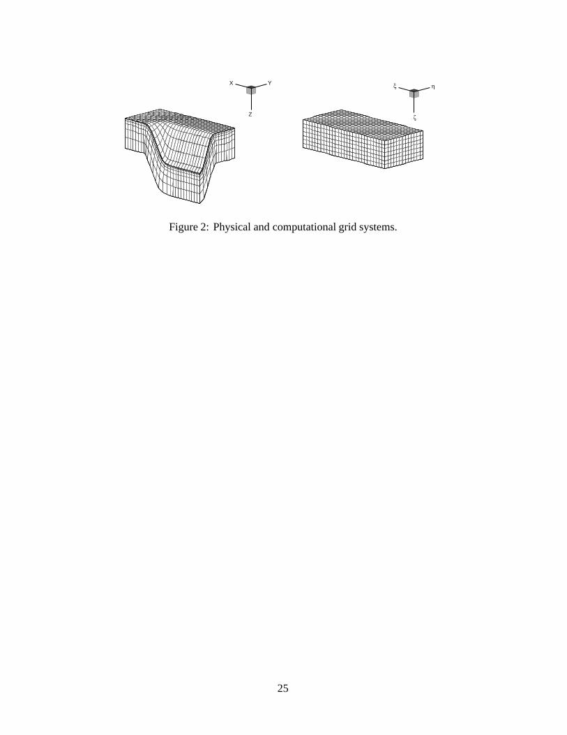
Figure 2: Physical and computational grid systems.

Figure 3: Variation of the local unit tangent along a �=const, �=const grid line.

Figure 4: Comparison of grooves generated with CW, pulsed and Q-switched lasers; (a) cross-sections along centerline, (b) cross-sections normal to laser scan direction.

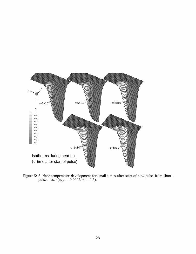
Figure 5: Surface temperature development for small times after start of new pulse from short-pulsed laser (�p�on = 0�0005, �p = 0�5).

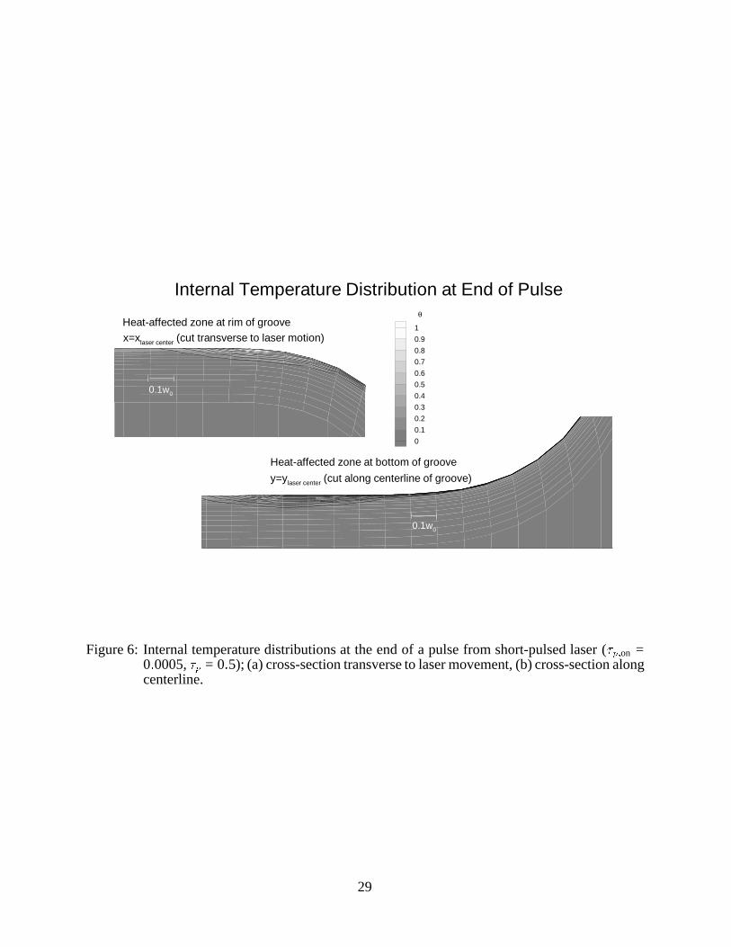
Figure 6: Internal temperature distributions at the end of a pulse from short-pulsed laser (�p�on =0�0005, �p = 0�5); (a) cross-section transverse to laser movement, (b) cross-section alongcenterline.

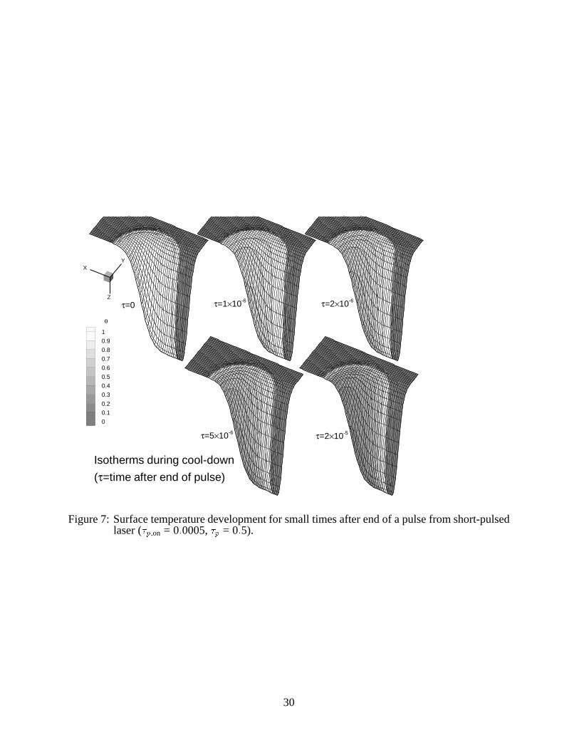
Figure 7: Surface temperature development for small times after end of a pulse from short-pulsedlaser (�p�on = 0�0005, �p = 0�5).

Figure 8: Surface temperature development for small times after start of new pulse from normal-pulsed laser (�p�on = 0�05, �p = 0�5).

Figure 9: Internal temperature distributions at the endpoint of a pulse from normal-pulsed laser(�p�on = 0�05, �p = 0�5); (a) cross-section transverse to laser movement, (b) cross-sectionalong centerline.

Figure 10: Surface temperature development for small times after start of new pulse from normal-pulsed laser (�p�on = 0�05, �p = 0�5).

Figure 11: Internal temperature distributions resulting from a CW laser; (a) cross-section transverseto laser movement, (b) cross-section along centerline.

23

���������� �������

Figure 1: Geometrical arrangement of laser and workpiece

24

X Y

Z

X Y

Z

ηξ

ζ

Figure 2: Physical and computational grid systems.

25

ζ=1

7

910

11

n

t

sl^

^

^

Figure 3: Variation of the local unit tangent along a �=const, �=const grid line.

26

0 1 2 3

0

2

4

6

y

(a) (b)

s

2 4 6 8 10 12

0

2

4

6

laser beam center at turn-on

Ste=2.5

z0=0

β∞=0.02

α=0.9

x

U=1.0

Nk=0.05

CW laser

Pulsed (tp,on/tp=0.1)

Q-switched (tp,on/tp=10-3)

Q-switched, U=1.5

at turn-off (CW and tp=0.5)

tp=0.5

CW

tp=0.75

tp=1.0

s

Figure 4: Comparison of grooves generated with CW, pulsed and Q-switched lasers; (a) cross-sections along centerline, (b) cross-sections normal to laser scan direction.

27

XY

Z

Isotherms during heat-up

(τ=time after start of pulse)

τ=1×10-7 τ=2×10-7 τ=5×10-7

τ=1×10-6 τ=5×10-6

θ

1

0.9

0.8

0.7

0.6

0.5

0.4

0.3

0.2

0.1

0

Figure 5: Surface temperature development for small times after start of new pulse from short-pulsed laser (�p�on = 0�0005, �p = 0�5).

28

0.1w0

Internal Temperature Distribution at End of Pulse

Heat-affected zone at rim of groove

Heat-affected zone at bottom of groove

0.1w0

x=xlaser center (cut transverse to laser motion)

y=ylaser center (cut along centerline of groove)

θ

1

0.9

0.8

0.7

0.6

0.5

0.4

0.3

0.2

0.1

0

Figure 6: Internal temperature distributions at the end of a pulse from short-pulsed laser (�p�on =0�0005, �p = 0�5); (a) cross-section transverse to laser movement, (b) cross-section alongcenterline.

29

XY

Z

Isotherms during cool-down

(τ=time after end of pulse)

τ=0 τ=1×10-6 τ=2×10-6

τ=5×10-6 τ=2×10-5

θ

1

0.9

0.8

0.7

0.6

0.5

0.4

0.3

0.2

0.1

0

Figure 7: Surface temperature development for small times after end of a pulse from short-pulsedlaser (�p�on = 0�0005, �p = 0�5).

30

XY

Zτ=.0005 τ=.0025τ=.0010

τ=.0050 τ=.0100

Isotherms during heat-up

(τ=time after start of pulse)

θ

1

0.9

0.8

0.7

0.6

0.5

0.4

0.3

0.2

0.1

0

Figure 8: Surface temperature development for small times after start of new pulse from normal-pulsed laser (�p�on = 0�05, �p = 0�5).

31

w0

Internal Temperature Distribution for Pulsed Operation

Heat-Affected Zone

along centerline

(y=ylaser center)

Heat-Affected Zone

for transverse cross-

section (x=xlaser center)

w0

1

0.9

0.8

0.7

0.6

0.5

0.4

0.3

0.2

0.1

0

Figure 9: Internal temperature distributions at the endpoint of a pulse from normal-pulsed laser(�p�on = 0�05, �p = 0�5); (a) cross-section transverse to laser movement, (b) cross-sectionalong centerline.

32

XY

Zτ=.000 τ=.002 τ=.005

τ=.010 τ=.030

Isotherms during cool-down

(τ=time after end of pulse)

θ

1

0.9

0.8

0.7

0.6

0.5

0.4

0.3

0.2

0.1

0

Figure 10: Surface temperature development for small times after start of new pulse from normal-pulsed laser (�p�on = 0�05, �p = 0�5).

33

Internal Temperature Distribution for CW OperationInternal Temperature Distribution for CW Operation

w0

Internal Temperature Distribution for CW Operation

w0

Heat-Affected Zone

for transverse cross-

section (x=xlaser center)

Heat-Affected Zone

along centerline

(y=ylaser center)

1

0.9

0.8

0.7

0.6

0.5

0.4

0.3

0.2

0.1

0

Figure 11: Internal temperature distributions resulting from a CW laser; (a) cross-section transverseto laser movement, (b) cross-section along centerline.

34